energy optimized scheduling for non-preemptive real...

Turk J Elec Eng & Comp Sci

(2017) 25: 3085 – 3096

c⃝ TUBITAK

doi:10.3906/elk-1508-37

Turkish Journal of Electrical Engineering & Computer Sciences

http :// journa l s . tub i tak .gov . t r/e lektr ik/

Research Article

Energy optimized scheduling for non-preemptive real-time systems

Vasanthamani KANNAIAN∗, Visalakshi PALANISAMYDepartment of Electronics and Communication Engineering, PSG College of Technology, Coimbatore, India

Received: 05.08.2015 • Accepted/Published Online: 09.12.2016 • Final Version: 30.07.2017

Abstract:Embedded systems have geared up their applications in the field of smart phones, mobile devices, automobiles,

and medical instrumentation. Along with the growth of technology, the functional requirements of the systems have also

grown multifold. To accommodate these ever increasing functional requirements, the hardware should be designed to

include the maximum capability, which in turn increases power consumption. Thus this has to be dynamically managed

using software techniques. The dynamic voltage and frequency scaling (DVFS) feature provided in most of the recent

processors has enabled power optimization through software. With this feature the processor operating frequency can

be reduced on the fly through software. This paper proposes two approaches. In the first one, the hyper period-based

method (HPBM), the slow down factor is calculated for the hyper period and the second method involves applying

uniform slow down with frequency inheritance (USFI) with a hyper plane exact test (HET). Both approaches aim to

calculate slow down factors for the tasks to be executed in the processors with the DVFS feature. The main objective of

this work is to provide energy optimized scheduling as well as to minimize the overheads in slow down factor calculations.

Key words: Real-time scheduling, non-preemptive tasks, energy efficiency, dynamic voltage and frequency scaling

1. Introduction

Energy consumption is a vital parameter in battery-operated portable mobile embedded systems [1,2]. The

lifetime of the battery between charges can be extended only if energy consumption is kept optimal. Modern

processors are equipped with power management techniques called dynamic voltage and frequency scaling

(DVFS) [3,4], which allows changes in the frequency of the processor on the fly through software. The power

consumption of the system depends on the voltage and the frequency of operation, which implies that reducing

either parameter reduces the power. The operating frequency can be reduced based on processor utilization.

The factor by which the frequency can be reduced depends on the worst case execution time and the available

slack time of the tasks. The ratio with which the frequency is reduced from the maximum frequency is called

the slow down factor. The calculated slow down factor should result in minimizing the energy consumption as

well as meet the time constraints of the tasks.

DVFS has enabled researchers to propose on-line and off-line techniques for energy efficient scheduling.

In hard real-time systems, especially in applications with intense I/O operations and safety critical applications,

non-preemptive tasks are widely used. These tasks exhibit benefits like low overheads and the need for

synchronization, as the number of context switches is less and the usage of the shared resources and data

are exclusive.

This paper deals with the energy efficient scheduling of non-preemptive periodic tasks in a uni-processor

∗Correspondence: [email protected]

3085

KANNAIAN and PALANISAMY/Turk J Elec Eng & Comp Sci

system that supports dynamic frequency adjustments. The first proposed method, hyper period-based method

(HPBM), is applied to both the earliest deadline first [5] and rate monotonic [5,6] algorithms. The second

proposed method, uniform slow down with frequency inheritance with reduced scheduling points set (USFI-

HET), is applied for the rate monotonic algorithm.

The rest of the paper is organized as follows: Section 2 reviews related research on energy optimized

scheduling, Section 3 introduces the system models, and Section 4 illustrates a motivational example. Section

5 describes the proposed techniques and Section 6 presents the results and discussions. Finally, Section 7

concludes this paper.

2. Related work

In real-time systems, tasks are classified as periodic, aperiodic, and sporadic. Enormous amounts of research

have been carried out for energy optimized scheduling of preemptive and non-preemptive periodic tasks and

aperiodic and sporadic tasks. Some works related to preemptive and non-preemptive tasks are discussed below.

2.1. Preemptive tasks

Shin et al. [7] used off-line and on-line techniques to calculate the slow down factors of the task. The off-

line technique calculated the lowest maximum processor speed while the on-line part dynamically varied the

processor speed or placed the processor in power down mode depending upon the status of the tasks. Aydin et

al. [8] calculated the processor speed for tasks based on their power characteristics. Aydin et al. [9] presented

both static and dynamic techniques for energy efficient scheduling. The static solution computed the optimal

speed at task level whereas the dynamic solution utilized the slack time of the tasks that have been completed

earlier than the WCET. Pillai and Shin [10] devised an algorithm to utilize the difference between the actual

execution time and the worst case execution time. The algorithm was called cycle conserving DVS and the slow

down factor for each task was calculated dynamically during every task release.

2.2. Non-preemptive tasks

Zhang and Chanson [11] proposed a dual speed algorithm for non-preemptive tasks. Normally the tasks run

at low speed and switch to high speed when the tasks were blocked. A dynamic reclaiming technique was also

presented to utilize the slack time of the task. A stack-based slow down algorithm was proposed by Jejurikar

and Gupta [12]. Two operating speeds for the processor were calculated: the base speed, which is the lowest

speed, and the highest speed, based on the blocking factors of the tasks. The highest speed is used whenever

a task is blocked. Jejurikar and Gupta suggested an algorithm, uniform slow down with frequency inheritance

[13]. The algorithm calculated the slow down factor starting from the task with the lowest deadline. The slow

down factor is calculated for each scheduling point considering the blocking time. Based on the calculated slow

down factor for the lowest period task, the slow down factor for the next task is calculated. The calculation

continued until the last task in the task set. Whenever a high priority task is blocked, the low priority task

inherits the slow down factor of the blocked high priority task and completes the task quickly. This reduces the

blocking time of the high priority task.

Energy aware scheduling is a demanding criterion in applications employing multi-core processors and

in server clusters. Sajid and Raza [14] proposed the ESHEFT algorithm to schedule the tasks in DVFS

enabled heterogeneous multi-core systems for optimizing turnaround time and energy consumption. Kumar

3086


and Raghunathan [15] proposed a hybrid approach for better energy saving using dynamic power management

(DPM) with sleep state and DVFS for virtualized server clusters.

3. System model

3.1. Task model

A synchronous task set T with N periodic tasks {τ1 , τ2 . . . τN } is considered to be scheduled in a hard

real-time system. A task is characterized by the tuple (C i , T i , D i), where C i is the worst-case execution time

of the task at the maximum speed of the processor, T i is the period of the task, and D i is the relative deadline

of the task. The task is ready for execution for the first time at t = 0 (zero offset) and then periodically for

every T i time units. The task requests its jth execution at time t i,j = (k − 1) × T i , where k = {1, 2, 3 . . . }.B i is the blocking time of the task and is computed using Eq. (1).

Bi = maxj>i

Cj (1)

3.2. Processor model

The supply voltage and frequency of the processor can be reduced whenever the processor is underutilized,

thereby reducing power consumption. The speed of the processor can be varied over a discrete range from fmin

to fmax . The ratio between the current processor frequency and the maximum processor frequency is called

the slow down factor. The slow down is also discrete and ranges from ηmin to 1. ηmin is the slow down factor

calculated based on the minimum frequency level with which the processor can be operated. The overhead in

switching of the frequency is assumed to be very minimal and included in the task execution time in earlier

works [11–13].

3.3. Energy model

The power consumption of the processor is calculated by Eq. (2) [16]:

P = CswfopV2dd, (2)

where Csw is the switching capacitance, fop is the frequency, and Vdd is the supply voltage. When the supply

voltage is changed from one level to another the overhead model [17] for time, tTRANS , is given by Eq. (3):

tTRANS =2CDD

IMAX|VDD2 − VDD1| , (3)

where CDD is the capacitance of the voltage converter, IMAX is the maximum output current of the converter,

and VDD2 and VDD1 are the voltage levels. The energy consumption by the CPU during the transition,

ETRANS−CPU , is given by Eq. (4)

ETRANS−CPU = P × tTRANS (4)

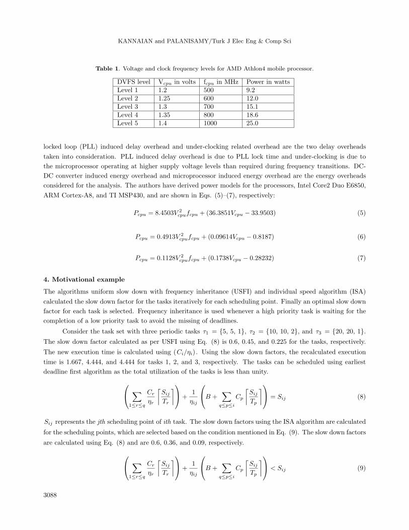
Table 1 shows the discrete voltage levels for the AMD Athlon4 DVS processor and it ranges from 1.2 to 1.4 V.

The energy and the transition time models mentioned in Eqs. (2)–(4) are generic and include only that

of the processor. Park et al. [18] have provided accurate modelling of the delay and energy overhead due to

DVFS. The authors have derived a power model in their work considering the delay and energy overhead. Phase

3087


Table 1. Voltage and clock frequency levels for AMD Athlon4 mobile processor.

DVFS level Vcpu in volts fcpu in MHz Power in wattsLevel 1 1.2 500 9.2Level 2 1.25 600 12.0Level 3 1.3 700 15.1Level 4 1.35 800 18.6Level 5 1.4 1000 25.0

locked loop (PLL) induced delay overhead and under-clocking related overhead are the two delay overheads

taken into consideration. PLL induced delay overhead is due to PLL lock time and under-clocking is due to

the microprocessor operating at higher supply voltage levels than required during frequency transitions. DC-

DC converter induced energy overhead and microprocessor induced energy overhead are the energy overheads

considered for the analysis. The authors have derived power models for the processors, Intel Core2 Duo E6850,

ARM Cortex-A8, and TI MSP430, and are shown in Eqs. (5)–(7), respectively:

Pcpu = 8.4503V 2cpufcpu + (36.3851Vcpu − 33.9503) (5)



4. Motivational example

The algorithms uniform slow down with frequency inheritance (USFI) and individual speed algorithm (ISA)

calculated the slow down factor for the tasks iteratively for each scheduling point. Finally an optimal slow down

factor for each task is selected. Frequency inheritance is used whenever a high priority task is waiting for the

completion of a low priority task to avoid the missing of deadlines.

Consider the task set with three periodic tasks τ1 = {5, 5, 1}, τ2 = {10, 10, 2}, and τ3 = {20, 20, 1}.The slow down factor calculated as per USFI using Eq. (8) is 0.6, 0.45, and 0.225 for the tasks, respectively.

The new execution time is calculated using (Ci/ηi). Using the slow down factors, the recalculated execution

time is 1.667, 4.444, and 4.444 for tasks 1, 2, and 3, respectively. The tasks can be scheduled using earliest

deadline first algorithm as the total utilization of the tasks is less than unity. ∑1≤r≤q

Cr

ηr

⌈Sij

Tr

⌉+1

ηij

B +∑

q≤p≤i

Cp

⌈Sij

Tp

⌉ = Sij (8)

Sij represents the jth scheduling point of ith task. The slow down factors using the ISA algorithm are calculated

for the scheduling points, which are selected based on the condition mentioned in Eq. (9). The slow down factors

are calculated using Eq. (8) and are 0.6, 0.36, and 0.09, respectively. ∑1≤r≤q

Cr

ηr

⌈Sij

Tr

⌉+1

ηij

B +∑

q≤p≤i

Cp

⌈Sij

Tp

⌉ < Sij (9)

3088


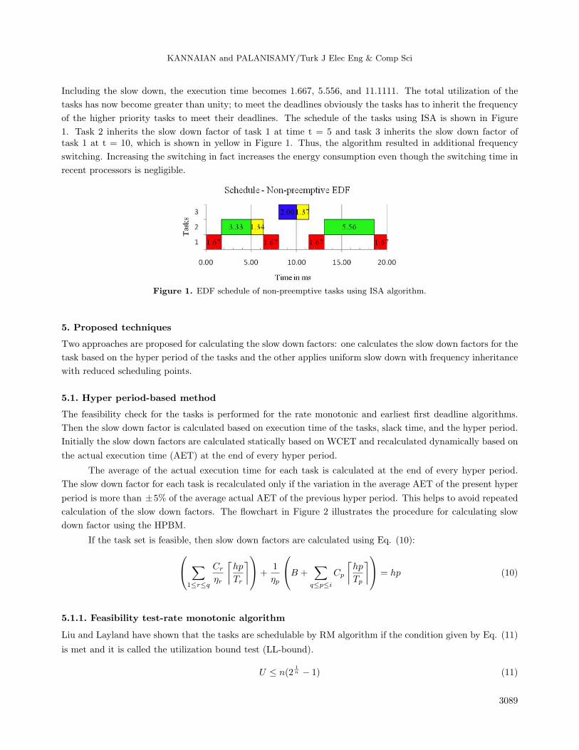
Including the slow down, the execution time becomes 1.667, 5.556, and 11.1111. The total utilization of the

tasks has now become greater than unity; to meet the deadlines obviously the tasks has to inherit the frequency

of the higher priority tasks to meet their deadlines. The schedule of the tasks using ISA is shown in Figure

1. Task 2 inherits the slow down factor of task 1 at time t = 5 and task 3 inherits the slow down factor oftask 1 at t = 10, which is shown in yellow in Figure 1. Thus, the algorithm resulted in additional frequency

switching. Increasing the switching in fact increases the energy consumption even though the switching time in

recent processors is negligible.

Figure 1. EDF schedule of non-preemptive tasks using ISA algorithm.

5. Proposed techniques

Two approaches are proposed for calculating the slow down factors: one calculates the slow down factors for the

task based on the hyper period of the tasks and the other applies uniform slow down with frequency inheritance

with reduced scheduling points.

5.1. Hyper period-based method

The feasibility check for the tasks is performed for the rate monotonic and earliest first deadline algorithms.

Then the slow down factor is calculated based on execution time of the tasks, slack time, and the hyper period.

Initially the slow down factors are calculated statically based on WCET and recalculated dynamically based on

the actual execution time (AET) at the end of every hyper period.

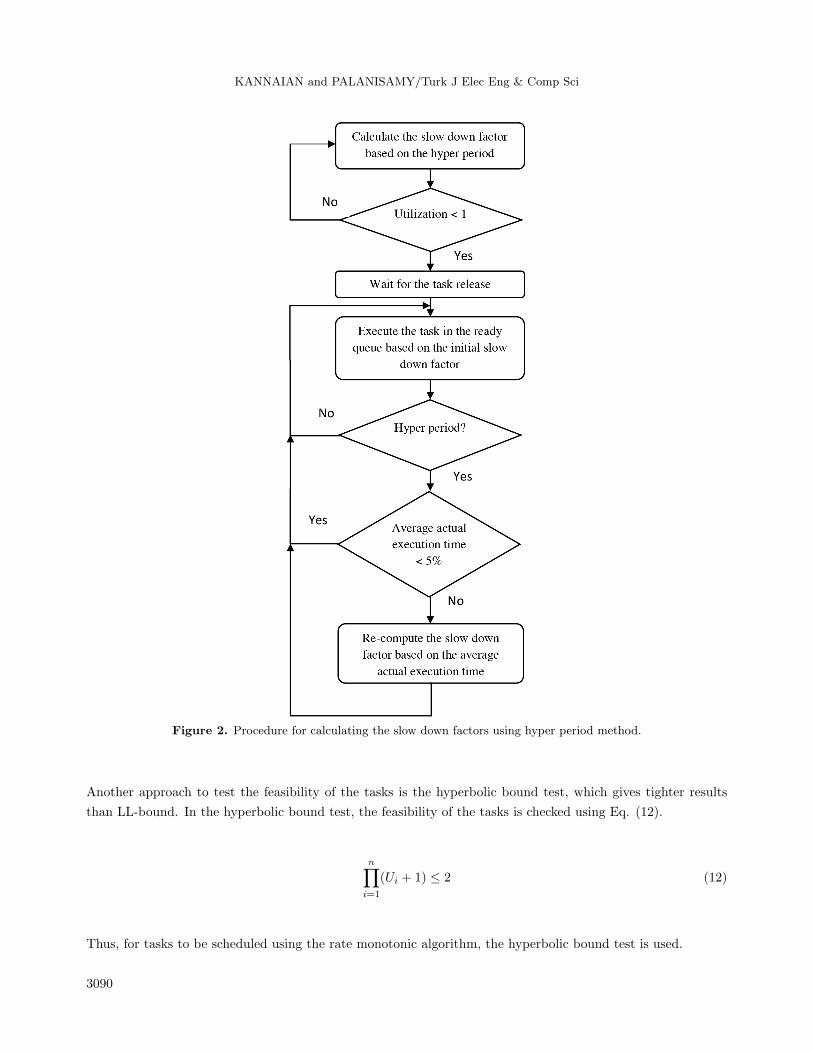
The average of the actual execution time for each task is calculated at the end of every hyper period.

The slow down factor for each task is recalculated only if the variation in the average AET of the present hyper

period is more than ±5% of the average actual AET of the previous hyper period. This helps to avoid repeated

calculation of the slow down factors. The flowchart in Figure 2 illustrates the procedure for calculating slow

down factor using the HPBM.

If the task set is feasible, then slow down factors are calculated using Eq. (10): ∑1≤r≤q

Cr

ηr

⌈hp

Tr

⌉+1

ηp

B +∑

q≤p≤i

Cp

⌈hp

Tp

⌉ = hp (10)

5.1.1. Feasibility test-rate monotonic algorithm

Liu and Layland have shown that the tasks are schedulable by RM algorithm if the condition given by Eq. (11)

is met and it is called the utilization bound test (LL-bound).

U ≤ n(21n − 1) (11)

3089


Figure 2. Procedure for calculating the slow down factors using hyper period method.

Another approach to test the feasibility of the tasks is the hyperbolic bound test, which gives tighter results

than LL-bound. In the hyperbolic bound test, the feasibility of the tasks is checked using Eq. (12).

n∏i=1

(Ui + 1) ≤ 2 (12)

Thus, for tasks to be scheduled using the rate monotonic algorithm, the hyperbolic bound test is used.

3090


Algorithm 1 To compute the slow down factor using the hyper period-based method

1: Input: T = {τ1, τ2 . . . τn } arranged in the non-decreasing order of their periods

2: Result: Slow down factors for the tasks in the task set.3: Calculate the maximum blocking time of the tasks

4: Initialization: q = 1

5: While q ≤ n do

Compute ηq by Eq. (10)

q = q + 1;

6: End while

5.1.2. Feasibility test-earliest deadline first algorithm

The feasibility test for the tasks under the EDF scheduling policy is given in Eq. (13).

∀i, i = 1, ..., n,Bi

Di+

i∑k=1

Ck

Dk≤ 1 (13)

5.2. Reduced scheduling points set for the rate monotonic algorithm

In the uniform slow down with frequency inheritance approach the slow down factor for each scheduling point

is calculated and the maximum of slow down factor for each task is taken into consideration. Eq. (8) is used

for calculating the slow down factor using USFI. The hyper-planes exact test (HET) [19] provides reduced

scheduling points based on Eq. (14). The USFI algorithm is applied to HET with reduced scheduling points.

The slow down factors calculated using USFI and USFI with HET yielded almost the same results, but the

time taken for the calculation was drastically reduced.

Hi(t) = Hi−1

(⌊t

pi

⌋pi

)∪Hi−1(t), (14)

where H0(t) = {t}

Lemma 1 The slow down factors can be calculated based on the hyper period.

Proof The periodic tasks should be checked for the feasibility of the schedule within their hyper period. For

the tasks with their deadline equal to that of the period, the tasks that arrived during the (i – 1)th instance

should be executed before the arrival of the ith instance. The available slack time within the hyper period of

the tasks is utilized for the tasks to reduce their speed of operation.

Lemma 2 The slow down factors can be calculated for the scheduling points using HET.

Proof The slow down factors are calculated for each scheduling point and the finally the maximum slow down

factor is assigned to the task. The maximum slow down factor results only for the last scheduling point. Hence

the slow down factors calculated using USFI and USFI-HET are similar.

3091


5.3. Computation time

The complexity is governed by Eq. (10) for the HPBM algorithm and by Eqs. (8) and (14) for USFI with HET.

Both algorithms calculate the slow down factor in linear time. The time complexity for the HPBM algorithm is

O(n). As the number of scheduling points taken for calculation is fixed, Eq. (8) calculates the slow down factor

in linear time and has “n” iterations. The time complexity for USFI with HET is O(n2).

6. Results and discussion

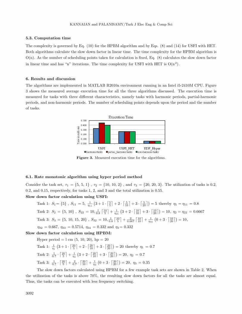
The algorithms are implemented in MATLAB R2010a environment running in an Intel i5-2410M CPU. Figure

3 shows the measured average execution time for all the three algorithms discussed. The execution time is

measured for tasks with three different characteristics, namely tasks with harmonic periods, partial-harmonic

periods, and non-harmonic periods. The number of scheduling points depends upon the period and the number

of tasks.

Figure 3. Measured execution time for the algorithms.

6.1. Rate monotonic algorithm using hyper period method

Consider the task set, τ1 = {5, 5, 1} , τ2 = {10, 10, 2} , and τ3 = {20, 20, 3}. The utilization of tasks is 0.2,

0.2, and 0.15, respectively, for tasks 1, 2, and 3 and the total utilization is 0.55.

Slow down factor calculation using USFI:

Task 1: S1= {5} , S11 = 5, 1η11

(3 + 1 ·

⌈55

⌉+ 2 ·

⌈510

⌉+ 3 ·

⌈520

⌉)= 5 thereby η1 = η11 = 0.8

Task 2: S2 = {5, 10} , S22 = 10, 10.8

⌈105

⌉+ 1

η21

(3 + 2 ·

⌈1010

⌉+ 3 ·

⌈1020

⌉)= 10, η2 = η22 = 0.6667

Task 3: S3 = {5, 10, 15, 20} , S32 = 10, 10.8

⌈105

⌉+ 2

0.667

⌈1010

⌉+ 1

η31

(0 + 3 ·

⌈1020

⌉)= 10,

η32 = 0.667, η33 = 0.5714, η34 = 0.332 and η3= 0.332

Slow down factor calculation using HPBM:

Hyper period = l cm (5, 10, 20), hp = 20

Task 1: 1η1

(3 + 1 ·

⌈205

⌉+ 2 ·

⌈2010

⌉+ 3 ·

⌈2020

⌉)= 20 thereby η1 = 0.7

Task 2: 10.7 ·

⌈205

⌉+ 1

η2

(3 + 2 ·

⌈2010

⌉+ 3 ·

⌈2020

⌉)= 20, η2 = 0.7

Task 3: 10.7 ·

⌈205

⌉+ 2

0.7 ·⌈2010

⌉+ 1

η3

(0 + 3 ·

⌈2020

⌉)= 20, η3 = 0.35

The slow down factors calculated using HPBM for a few example task sets are shown in Table 2. When

the utilization of the tasks is above 70%, the resulting slow down factors for all the tasks are almost equal.

Thus, the tasks can be executed with less frequency switching.

3092


Table 2. Slow down factor calculation using HPBM.

S. no. Task set Utilization Slow down factors1 τ1 = {100, 100, 30} , τ2 = {125, 125, 15} ,

τ3 = {140, 140, 30} , τ4 = {170, 170, 7} ,τ5 = {200, 200, 15}

0.726 0.7507, 0.7507,0.7504, 0.7504,0.7492

2 τ1 = {5, 5, 1} , τ2 = {10, 10, 2} , τ3 = {20, 20, 3} 0.55 0.7, 0.7, 0.353 τ1 = {5, 5, 1} , τ2 = {10, 10, 3} , τ3 = {20, 20, 3} 0.65 0.8, 0.8, 0.44 τ1 = {5, 5, 1} , τ2 = {10, 10, 2} , τ3 = {20, 20, 2} 0.5 0.6, 0.6, 0.3

6.2. Rate monotonic algorithm using USFI with reduced scheduling points

Slow down factor calculation using USFI:

Task 1: S1= {5} , S11 = 5, 1η11

(3 + 1 ·

⌈55

⌉+ 2 ·

⌈510

⌉+ 3 ·

⌈520

⌉)= 5 thereby η1 = η11 = 0.8

Task 2: S2 = {5, 10} , S22 = 10, 10.8

⌈105

⌉+ 1

η21

(3 + 2 ·

⌈1010

⌉+ 3 ·

⌈1020

⌉)= 10, η2 = η22 = 0.6667

Task 3: S3 = {15, 20} , S31 = 15, 10.8

⌈155

⌉+ 2

0.667

⌈1510

⌉+ 1

η31

(0 + 3 ·

⌈1520

⌉)= 15,

η31 = 0.5714 and η32 = 0.332, η3= 0.332

Table 3 shows the percentage of reduction in the scheduling points used for calculating the slow down

factors using HET. The percentage will be more if the tasks are non-harmonic.

Table 3. Performance of slow down factor calculation using USFI-HET.

S. no. Task set Nature of tasks Reduced by1 τ1 = {5, 5, 1} , τ2 = {14, 14, 2} , τ3 = {30, 30, 3} Partially harmonic 25%2 τ1 = {3, 3, 1} , τ2 = {8, 8, 2} , τ3 = {13, 13, 3} Non-harmonic 33.33%

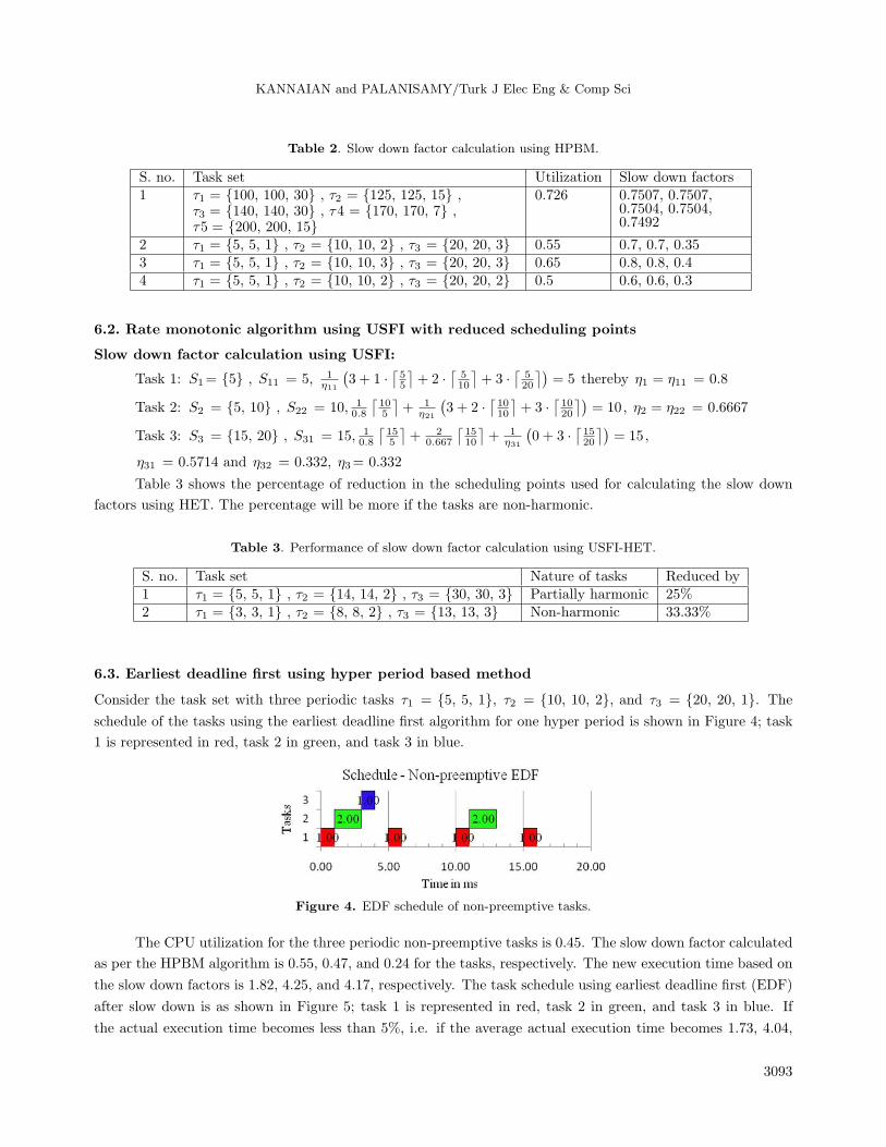
6.3. Earliest deadline first using hyper period based method

Consider the task set with three periodic tasks τ1 = {5, 5, 1}, τ2 = {10, 10, 2}, and τ3 = {20, 20, 1}. The

schedule of the tasks using the earliest deadline first algorithm for one hyper period is shown in Figure 4; task

1 is represented in red, task 2 in green, and task 3 in blue.

Figure 4. EDF schedule of non-preemptive tasks.

The CPU utilization for the three periodic non-preemptive tasks is 0.45. The slow down factor calculated

as per the HPBM algorithm is 0.55, 0.47, and 0.24 for the tasks, respectively. The new execution time based on

the slow down factors is 1.82, 4.25, and 4.17, respectively. The task schedule using earliest deadline first (EDF)

after slow down is as shown in Figure 5; task 1 is represented in red, task 2 in green, and task 3 in blue. If

the actual execution time becomes less than 5%, i.e. if the average actual execution time becomes 1.73, 4.04,

3093


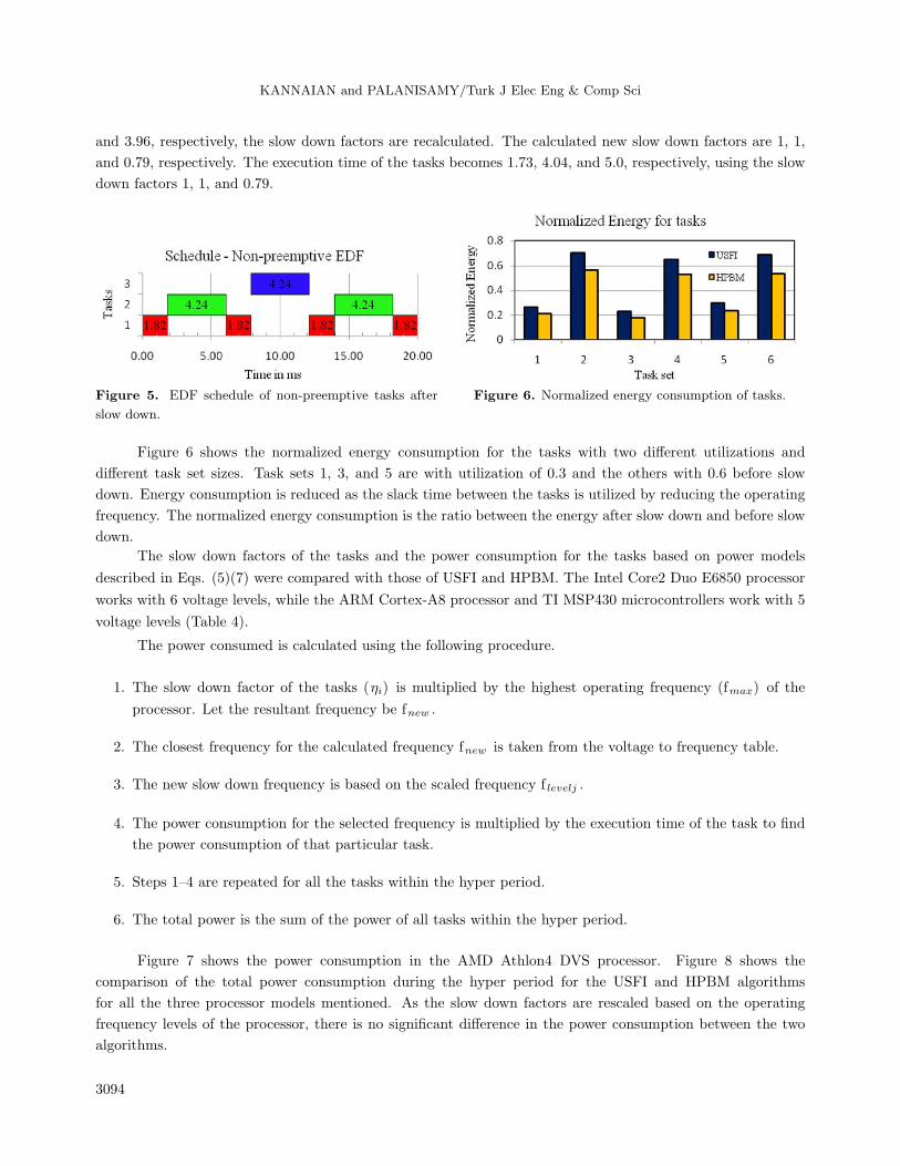
and 3.96, respectively, the slow down factors are recalculated. The calculated new slow down factors are 1, 1,

and 0.79, respectively. The execution time of the tasks becomes 1.73, 4.04, and 5.0, respectively, using the slow

down factors 1, 1, and 0.79.

Figure 5. EDF schedule of non-preemptive tasks after

slow down.

Figure 6. Normalized energy consumption of tasks.

Figure 6 shows the normalized energy consumption for the tasks with two different utilizations and

different task set sizes. Task sets 1, 3, and 5 are with utilization of 0.3 and the others with 0.6 before slow

down. Energy consumption is reduced as the slack time between the tasks is utilized by reducing the operating

frequency. The normalized energy consumption is the ratio between the energy after slow down and before slow

down.

The slow down factors of the tasks and the power consumption for the tasks based on power models

described in Eqs. (5)(7) were compared with those of USFI and HPBM. The Intel Core2 Duo E6850 processor

works with 6 voltage levels, while the ARM Cortex-A8 processor and TI MSP430 microcontrollers work with 5

voltage levels (Table 4).

The power consumed is calculated using the following procedure.

1. The slow down factor of the tasks (ηi) is multiplied by the highest operating frequency (fmax) of the

processor. Let the resultant frequency be fnew .

2. The closest frequency for the calculated frequency fnew is taken from the voltage to frequency table.

3. The new slow down frequency is based on the scaled frequency f levelj .

4. The power consumption for the selected frequency is multiplied by the execution time of the task to find

the power consumption of that particular task.

5. Steps 1–4 are repeated for all the tasks within the hyper period.

6. The total power is the sum of the power of all tasks within the hyper period.

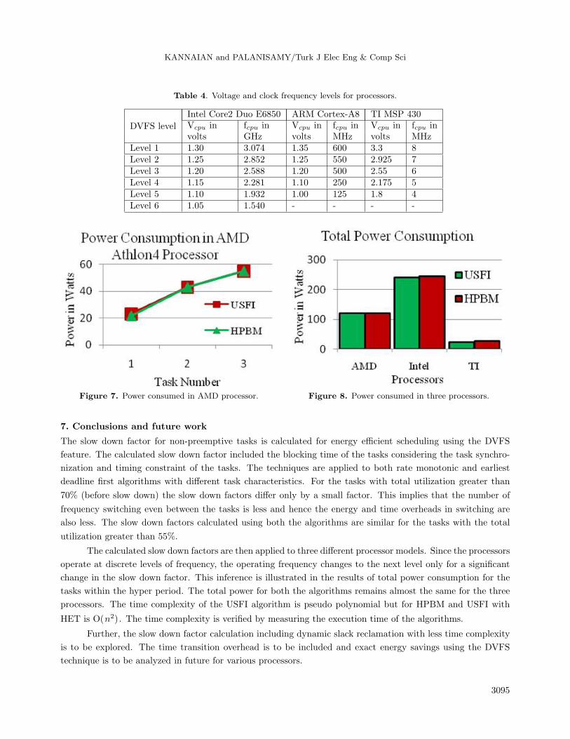
Figure 7 shows the power consumption in the AMD Athlon4 DVS processor. Figure 8 shows the

comparison of the total power consumption during the hyper period for the USFI and HPBM algorithms

for all the three processor models mentioned. As the slow down factors are rescaled based on the operating

frequency levels of the processor, there is no significant difference in the power consumption between the two

algorithms.

3094


Table 4. Voltage and clock frequency levels for processors.

DVFS level

Intel Core2 Duo E6850 ARM Cortex-A8 TI MSP 430Vcpu in fcpu in Vcpu in fcpu in Vcpu in fcpu involts GHz volts MHz volts MHz

Level 1 1.30 3.074 1.35 600 3.3 8Level 2 1.25 2.852 1.25 550 2.925 7Level 3 1.20 2.588 1.20 500 2.55 6Level 4 1.15 2.281 1.10 250 2.175 5Level 5 1.10 1.932 1.00 125 1.8 4Level 6 1.05 1.540 - - - -

Figure 7. Power consumed in AMD processor. Figure 8. Power consumed in three processors.

7. Conclusions and future work

The slow down factor for non-preemptive tasks is calculated for energy efficient scheduling using the DVFS

feature. The calculated slow down factor included the blocking time of the tasks considering the task synchro-

nization and timing constraint of the tasks. The techniques are applied to both rate monotonic and earliest

deadline first algorithms with different task characteristics. For the tasks with total utilization greater than

70% (before slow down) the slow down factors differ only by a small factor. This implies that the number of

frequency switching even between the tasks is less and hence the energy and time overheads in switching are

also less. The slow down factors calculated using both the algorithms are similar for the tasks with the total

utilization greater than 55%.

The calculated slow down factors are then applied to three different processor models. Since the processors

operate at discrete levels of frequency, the operating frequency changes to the next level only for a significant

change in the slow down factor. This inference is illustrated in the results of total power consumption for the

tasks within the hyper period. The total power for both the algorithms remains almost the same for the three

processors. The time complexity of the USFI algorithm is pseudo polynomial but for HPBM and USFI with

HET is O(n2). The time complexity is verified by measuring the execution time of the algorithms.

Further, the slow down factor calculation including dynamic slack reclamation with less time complexity

is to be explored. The time transition overhead is to be included and exact energy savings using the DVFS

technique is to be analyzed in future for various processors.

3095


References

[1] Marwedel P. Embedded System Design: Embedded Systems Foundations of Cyber-Physical Systems. 2nd ed. New

York, NY, USA: Springer, 2010.

[2] Vahid F, Givargis T. Embedded System Design – A Unified Hardware/Software Introduction. 3rd ed. New Delhi,

India: Wiley, 2009.

[3] Bhatti K, Belleudy C, Auguin M. Power management in real time embedded systems through online and adaptive

interplay of DPM and DVFS policies. In: IEEE Embedded and Ubiquitous Computing Conference; 11–13 December

2010; Hong Kong: IEEE. pp. 184-191.

[4] Mittal S. A survey of techniques for improving energy efficiency in embedded computing systems. Int J Comp A

Eng Technol 2014; 6: 440-459.

[5] Liu C, Layland J. Scheduling algorithms for multiprogramming in a hard real-time environment. ACM J 1973; 20:

46-61.

[6] Lehoczky J, Sha L, Ding Y. The rate monotonic scheduling algorithm: exact characterization and average case

behaviour. In: IEEE Real Time Systems Symposium; 5–7 December 1989; Santa Monica, CA: IEEE. pp. 166-171.

[7] Shin Y, Choi K, Sakurai T. Power optimization of real-time embedded systems on variable speed processors. In:

IEEE/ACM Computer-aided design conference; 5–9 November 2000; San Jose, CA, USA: IEEE. pp. 365-368.

[8] Aydin H, Melhem R, Mosse D, Mejsıa-Alvarez P. Determining optimal processor speeds for periodic real-time tasks

with different power characteristics. In: IEEE Real-Time Systems Euromicro Conference; 13–15 June 2001; Delft:

IEEE. pp. 225-232.

[9] Aydin H, Melhem R, Mosse D, Mejsıa-Alvarez P. Dynamic and aggressive scheduling techniques for power-aware

real-time systems. In: IEEE Real-Time Systems Symposium; 3-6 December 2001; London, UK: IEEE. pp. 95-105.

[10] Pillai P, Shin KG. Real-time dynamic voltage scaling for low power embedded operating systems. In: ACM SIGOPS

Operating Systems Review; 2001; New York, USA: ACM. pp. 89-102.

[11] Zhang F, Chanson ST. Blocking-aware processor voltage scheduling for real-time tasks. ACM T Embed Comput S

2004; 3: 307-335.

[12] Jejurikar R, Gupta RK. Energy aware non-preemptive scheduling for hard real-time systems. In: IEEE Real-Time

Systems Euromicro Conference; 6–8 July 2005; Spain: IEEE. pp. 21-30.

[13] Jejurikar R, Gupta R. Energy aware task scheduling with task synchronization for embedded real time systems.

IEEE T Comp Aid D 2006; 25: 1024-1037.

[14] Sajid MO, Raza ZA. Energy-aware stochastic scheduling with precedence-constraints on DVFS-enabled processors.

Turk J Elec Eng & Comp Sci 2015; 24: 4117-4128.

[15] Kumar M R, Raghunathan S. Power management using dynamic power state transitions and dynamic voltage

frequency scaling controls in virtualized server clusters. Turk J Elec Eng & Comp Sci 2016; 24: 2290-2306.

[16] Suleiman D, Ibrahim M, Hamarash I. Dynamic voltage frequency scaling (DVFS) for microprocessors power and

energy reduction. In: Electrical and Electronics Engineering Conference; December 2005.

[17] Shao Z, Meng W, Chen Y, Xue C, Qiu M, Yang LT, Sha EH. Real-time dynamic voltage loop scheduling for

multi-core embedded systems. IEEE T Circuits Syst 2007; 54: 445-449.

[18] Park S, Park J, Shin D, Wang Y, Xie Q, Pedram M, Chang N. Accurate modeling of the delay and energy overhead

of dynamic voltage and frequency scaling in modern microprocessors. IEEE T Comput Aid D 2013; 32: 695-708.

[19] Bini E, Buttazzo GC. Schedulability analysis of periodic fixed priority systems. IEEE T Comput 2004; 53: 1462-

1473.

3096

http://dx.doi.org/10.1109/EUC.2010.35



http://dx.doi.org/10.1504/IJCAET.2014.065419

http://dx.doi.org/10.1504/IJCAET.2014.065419

http://dx.doi.org/10.1145/321738.321743

http://dx.doi.org/10.1145/321738.321743

http://dx.doi.org/10.1109/REAL.1989.63567


http://dx.doi.org/10.1109/EMRTS.2001.934038





http://dx.doi.org/10.1145/993396.993401

http://dx.doi.org/10.1145/993396.993401

http://dx.doi.org/10.1109/ECRTS.2005.13

http://dx.doi.org/10.1109/ECRTS.2005.13

http://dx.doi.org/10.1109/TCAD.2005.855964


http://dx.doi.org/10.3906/elk-1505-112






http://dx.doi.org/10.1109/TC.2004.103

http://dx.doi.org/10.1109/TC.2004.103

energy optimized scheduling for non-preemptive real...

Documents