energy regulator supply restoration time

energies

Article

Energy Regulator Supply Restoration Time

Mohd Ikhwan Muhammad Ridzuan 1,* and Sasa Z. Djokic 2

1 Faculty of Electrical & Electronics Engineering, Universiti Malaysia Pahang, Pekan 26600, Malaysia2 Institute for Energy System, The University of Edinburgh, Edinburgh EH9 3DW, UK; [email protected]* Correspondence: [email protected]; Tel.: +60-9-424-6026

Received: 30 January 2019; Accepted: 26 February 2019; Published: 19 March 2019��

Abstract: In conventional reliability analysis, the duration of interruptions relied on the inputparameter of mean time to repair (MTTR) values in the network components. For certain criteriawithout network automation, reconfiguration functionalities and/or energy regulator requirementsto protect customers from long excessive duration of interruptions, the use of MTTR input seemsreasonable. Since modern distribution networks are shifting towards smart grid, some factorsmust be considered in the reliability assessment process. For networks that apply reconfigurationfunctionalities and/or network automation, the duration of interruptions experienced by a customerdue to faulty network components should be addressed with an automation switch or manual actiontime that does not exceed the regulator supply restoration time. Hence, this paper introducesa comprehensive methodology of substituting MTTR with maximum action time required toreplace/repair a network component and to restore customer duration of interruption with maximumnetwork reconfiguration time based on energy regulator supply requirements. The Monte Carlosimulation (MCS) technique was applied to medium voltage (MV) suburban networks to estimatesystem-related reliability indices. In this analysis, the purposed method substitutes all MTTR valueswith time to supply (TTS), which correspond with the UK Guaranteed Standard of Performance(GSP-UK), by the condition of the MTTR value being higher than TTS value. It is nearly impossiblefor all components to have a quick repairing time, only components on the main feeder were selectedfor time substitution. Various scenarios were analysed, and the outcomes reflected the applicabilityof reconfiguration and the replace/repair time of network component. Theoretically, the networkreconfiguration (option 1) and component replacement (option 2) with the same amount of repairtime should produce exactly the same outputs. However, in simulation, these two options yielddifferent outputs in terms of number and duration of interruptions. Each scenario has its advantagesand disadvantages, in which the distribution network operators (DNOs) were selected based on theiroperating conditions and requirements. The regulator reliability-based network operation is moreapplicable than power loss-based network operation in counties that employed energy regulatorrequirements (e.g., GSP-UK) or areas with many factories that required a reliable continuous supply.

Keywords: reliability; network reconfiguration; time to supply; guaranteed standard of performance

1. Introduction

The reliability performance of distribution networks incorporates all possible contingenciesassociated with all power components in the network, including distribution feeders and protectionsystems. Reliability performance of the network is mostly related to maintaining the power supplyto the customer. Apart from maintaining the voltage level within permissible limits and minimisingthe feeder losses, network reconfiguration is able to maintain an adequate level of reliability set bythe energy regulator [1,2]. In addition, the network operation must adhere to the P2/6 EngineeringRecommendation [3] that suggests transfer capacity from alternative sources by certain maximumtimes based on class of group demands.

Energies 2019, 12, 1051; doi:10.3390/en12061051 www.mdpi.com/journal/energies

http://www.mdpi.com/journal/energies

http://www.mdpi.com

https://orcid.org/0000-0002-0549-9221

http://www.mdpi.com/1996-1073/12/6/1051?type=check_update&version=1

http://dx.doi.org/10.3390/en12061051

http://www.mdpi.com/journal/energies

Energies 2019, 12, 1051 2 of 16

In general, the structure of a distribution network reflects a meshed configuration that normallyoperates radially with the support of another supply point, either a primary substation or a reflectioncentre. A reflection centre resembles a closed-loop arrangement that guarantees the supply of allconnected feeders. With the advent of remote control of switches and circuit breakers, distributionnetwork operators (DNOs) are able to control network reconfiguration easily and further boost systemautomation. Network reconfiguration also relieves the overloading of the network components.Feeder reconfiguration is performed by opening switches/breakers (normally closed) that are closedto the faulty part of the network and closing switches/breakers (normally open) located at the end ofthe feeder network [4–7]. Switching is performed in such a way that the network radial is maintainedand all loads are energised. A normally open switch/breaker is closed to transfer a load from onefeeder to another, while an appropriate switch/breaker is opened to restore the radial structure.

Another conventional method of restoring customer interruption is by repairing or replacingthe faulty network component [8–11]. The selection of either repairing or replacing a faulty networkcomponent depends on the class of group demand outage, types of network components, networkcomponent availability, transportation, geographical area of faulty area, and others. For transformeroutage in group of demand type class B [3], supply to customer must be restored by maximum 3 h,which can only be performed via replacement. Outage originated from a faulty fuse is typically below1 MW (class A [3]) and no definite restoration time in [3]. However, the restoration of faulty fuses mustbe performed within maximum 3 h based on [1].

In the last decade, various objectives have been used for network reconfiguration. The objectiveor the aim of network reconfiguration can either be single or multiobjective. The varieties of singleobjectives are minimisation of power losses or energy losses, total network cost, voltage deviation,benefit/cost ratio and voltage sags. Multiobjectives combine two or more single objectives in a networkreconfiguration. Power loss minimisation [12–16] and voltage profile [17–20] are conventionallyemployed for network reconfiguration with less attention towards network reliability [18,21].

The literature pertaining to reliability-based reconfiguration, though in abundance, is not inclinedtoward energy regulator requirements, which substantially improves interruption frequency andduration. Although reducing interruption frequency and power loss is interrelated, the objectivediffers. In reliability, the main purpose is to minimise frequency of customer interruption regardless ofload demand (maximum, average or minimum), whereas in power loss, saving maximum load demand(to minimise load loss) is the priority than protecting customers with minimum load. In addressingthis challenge, this paper proposes an alternative approach in using new restoration times called timeto supply (TTS) for realistic evaluation of distribution reliability performance.

2. Input Parameters

2.1. Suburban MV Network

A typical UK suburban distribution network was considered in the analysis (see Figure 1).The radial type of power distribution network delivers power from the main branch to sub-branches,then splitting out from the sub-branches again. This appears to be the cheapest, but least reliablenetwork configuration. Tables 1 and 2 present the parameters of UK suburban network.

Energies 2019, 12, 1051 3 of 16Energies 2019, 12, x FOR PEER REVIEW 3 of 16

Figure 1. Typical distribution network configuration supplying suburban residential load [22–27].

A typical UK suburban distribution network was considered in the analysis (see Figure 1). The radial type of power distribution network delivers power from the main branch to sub-branches, then splitting out from the sub-branches again. This appears to be the cheapest, but least reliable network configuration. Tables 1 and 2 present the parameters of UK suburban network.

Table 1. Parameters of Typical 11, 0.4, and 0.23 kV Feeders [22,28–30].

Operating Voltage (kV)

Feeder Type Id. Cross Section (mm2)

Resistance/km Reactance/km (p.u. on 100 MVA)

11 Overhead Lines or Mixed

R 150 0.11259 0.18363 S 100 0.14658 0.26189

0.4 D 95 0.32 0.075 E 50 0.443 0.076 H 95 0.32 0.085

0.23 L 35 0.851 0.041

Table 2. Parameters of Typical MV/LV Transformers [22,28,30–32].

Operating Voltage

(kV)

Vector Group

Rating (MVA)

Resistance Reactance Tap Range Tap Step

(p.u. on 100 MVA) Min Max

33/11 Dyn11 5 0.14 1.3 0.85 1.045 0.0143 11/0.4 Dyn11 0.2 7.5 22.5 0.95 1.05 0.025

2.2. Mean Fault Rates and Mean Time to Repair (MTTR)

Mean fault rates and MTTR are the two basic inputs required for system reliability assessments. In the literature, the reported values of these two input data vary in wide ranges (based on the characteristics and location of network, types and features of power components, as well as their

Figure 1. Typical distribution network configuration supplying suburban residential load [22–27].

Table 1. Parameters of Typical 11, 0.4, and 0.23 kV Feeders [22,28–30].

Operating Voltage (kV) Feeder Type Id. Cross Section (mm2)Resistance/km Reactance/km

(p.u. on 100 MVA)

11

Overhead Lines or Mixed

R 150 0.11259 0.18363

S 100 0.14658 0.26189

0.4

D 95 0.32 0.075

E 50 0.443 0.076

H 95 0.32 0.085

0.23 L 35 0.851 0.041

Table 2. Parameters of Typical MV/LV Transformers [22,28,30–32].

Operating Voltage (kV) Vector Group Rating (MVA)Resistance Reactance Tap Range

Tap Step(p.u. on 100 MVA) Min Max

33/11 Dyn11 5 0.14 1.3 0.85 1.045 0.0143

11/0.4 Dyn11 0.2 7.5 22.5 0.95 1.05 0.025

2.2. Mean Fault Rates and Mean Time to Repair (MTTR)

Mean fault rates and MTTR are the two basic inputs required for system reliability assessments.In the literature, the reported values of these two input data vary in wide ranges (based on thecharacteristics and location of network, types and features of power components, as well as theiroperating conditions). Table 3 presents the statistics of mean fault rates and mean repair times obtainedfrom two main sources: UK-related values reported in [33] and from other sources [34–41].

Energies 2019, 12, 1051 4 of 16

Table 3. Mean Fault Rates and MTTR of Power Components.

Power Component Voltage Level (kV)Mean Fault Rate

λmean (Faults/Year)MTTR

µmean (Hours/Fault)

[33] [34–41] [33] [34–41]

Overhead Lines

<11 0.168 0.21 5.7 -

11 0.091 0.1 9.5 -

33 0.034 0.1 20.5 55

Cables

<11 0.159 0.19 6.9 85

11 0.051 0.05 56.2 48

33 0.034 0.05 201.6 128

Transformers

11/0.4 0.002 0.014 75 120

33/0.4 0.01 0.014 205.5 120

33/11 0.01 0.009 205.5 125

Buses

0.4 - 0.005 - 24

11 - 0.005 - 120

>11 - 0.08 - 140

Circuit Breakers

0.4 - 0.005 - 36

11 0.0033 0.005 120.9 48

33 0.0041 - 140 52

Fuses <11 0.0004 - 35.3 -

2.3. Fault Types

The classification of customer interruption into short interruption (SI) and long interruption (LI)is impossible without, for instance, modelling the applied protection systems. One simple way tomake a clear distinction between short and long supply interruptions of customers is by defining auniform distribution and linking it to the system reliability assessment procedure. For that purpose,past recordings collected from 14 UK DNOs between 2005 and 2009 [42] were analysed, in which54% of supply interruption events were caused by temporary faults (i.e., SI), and 46% were due topermanent faults (i.e., LI).

2.4. Guaranteed Standard of Performance

The energy regulator has specified certain requirements for the duration and the numberof interruptions in order to protect domestic (i.e., residential) and non-domestic customers (i.e.,customers without special contract or agreement with the DNOs regarding LI) from excessive LIevents. References depicted in [1] and [28] refer to the main UK statutory instrument, specifyingthe permissible supply restoration times for up to 5000 customers and more than 5000 customers,respectively. This is illustrated in Table 4 (normal system operating conditions), along with thecorresponding compensations that DNOs pay directly to the customers (and not to the regulator),if the supply is not restored within the specified time [1] and [28].

Energies 2019, 12, 1051 5 of 16

Table 4. The UK Guaranteed Standard of Performance (GSP-UK).

Supply Restoration Time Compensation Paid to:

No. of Customers Interrupted Maximum Supply Restoration Time Domestic Customers Non-Domestic Customers

<500018 h £54 £108

After each succeeding 12 h £27

≥500024 h £54 £108

After each succeeding 12 h £27

Maximum £216

Multiple Interruptions Compensation (all customers)

Four or more interruptions (≥4),each lasting at least three hours (≥3 h) £54

3. Reliability Methodologies

Probabilistic reliability assessment procedures seem to suit the analysis of system reliabilityperformance, particularly in terms of their ability to model stochastic and inherently unpredictablevariations of input parameters and data (e.g., fault rates and repair times) with their assumedprobability distributions. The approaches of the probabilistic reliability assessment model providea wide range of variations of practically all input parameters and data in one or a fewsimulation/calculation setups, without repeating the calculation after an input data is modified.

Although the probabilistic reliability assessment procedures are more difficult to implement(particularly in complex large-scale systems), they provide accurate and detailed outputs. The mostfrequently used probabilistic reliability assessment approach is the Monte Carlo simulation (MCS) [43–47].Aside from network modelling, conventional MCS analysis requires statistical information on fault rates andMTTR of faulted power components as input data. Network models and fault rates of power componentsare used to establish customers experiencing interruptions (and the frequency), whereas MTTR of faultedcomponents and network protection, reconfiguration, switching and alternative supply functionalities areused to estimate the duration of corresponding supply interruptions. The outputs of MCS analysis arereliability indices that reflect probability distributions with the corresponding mean values.

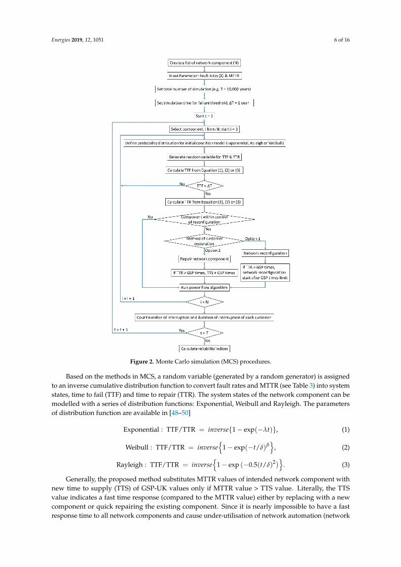
3.1. Monte Carlo Simulation (MCS) Procedures

In any power system reliability procedures, MTTR is used to define the restoration times ofnetwork components that directly have an impact on the duration of interruption. In some cases,where network automation is unavailable (network reconfiguration) or in the absence of regulatorysupply requirements (in some nations) on distribution networks, it is indeed realistic to use MTTRvalues. Nevertheless, in a country that applies regulatory supply requirements, the function of MTTRas input data may result in significant overestimation of reliability performance. Thus, DNOs shouldconsider a new method to assess the duration of interruption by correlating with regulatory supplyrequirement time. Accordingly, this section presents a new methodology (see Figure 2) of assessingduration of interruption realistically, based on GSP-UK restoration times.


Figure 2. Monte Carlo simulation (MCS) procedures.

In any power system reliability procedures, MTTR is used to define the restoration times of network components that directly have an impact on the duration of interruption. In some cases, where network automation is unavailable (network reconfiguration) or in the absence of regulatory supply requirements (in some nations) on distribution networks, it is indeed realistic to use MTTR values. Nevertheless, in a country that applies regulatory supply requirements, the function of MTTR as input data may result in significant overestimation of reliability performance. Thus, DNOs should consider a new method to assess the duration of interruption by correlating with regulatory supply requirement time. Accordingly, this section presents a new methodology (see Figure 2) of assessing duration of interruption realistically, based on GSP-UK restoration times.

Based on the methods in MCS, a random variable (generated by a random generator) is assigned to an inverse cumulative distribution function to convert fault rates and MTTR (see Table 3) into system states, time to fail (TTF) and time to repair (TTR). The system states of the network component can be modelled with a series of distribution functions: Exponential, Weibull and Rayleigh. The parameters of distribution function are available in [48–50]

Exponential: TTF/TTR = , (1) { })exp(1 tinverse λ−−

Figure 2. Monte Carlo simulation (MCS) procedures.

Based on the methods in MCS, a random variable (generated by a random generator) is assignedto an inverse cumulative distribution function to convert fault rates and MTTR (see Table 3) into systemstates, time to fail (TTF) and time to repair (TTR). The system states of the network component can bemodelled with a series of distribution functions: Exponential, Weibull and Rayleigh. The parametersof distribution function are available in [48–50]

Exponential : TTF/TTR = inverse{1− exp(−λt)}, (1)

Weibull : TTF/TTR = inverse{

1− exp(−t/δ)β}

, (2)

Rayleigh : TTF/TTR = inverse{

1− exp (−0.5(t/δ)2)}

. (3)

Generally, the proposed method substitutes MTTR values of intended network component withnew time to supply (TTS) of GSP-UK values only if MTTR value > TTS value. Literally, the TTSvalue indicates a fast time response (compared to the MTTR value) either by replacing with a newcomponent or quick repairing the existing component. Since it is nearly impossible to have a fastresponse time to all network components and cause under-utilisation of network automation (network

Energies 2019, 12, 1051 7 of 16

reconfiguration), only components on the main feeder (carrying a high current that may affect manycustomers) are selected to replace MTTR values with TTR values (option 2). To compare the practicalityof option 2 with complete network automation, option 1, network reconfiguration, was generated.In option 1, the network component fault/interruption time adheres to the exact values of MTTR, whilethe customer restoration time is shorted by the GSP-UK duration limit via network reconfiguration.In other word, customers experience outages through the normal path of electrical supply and theduration of outage experienced by the same customer is shortened by rerouting the electrical supplythrough the network reconfiguration until the faulty component is repaired/replaced.

3.2. Considered Scenarios

In Table 5, scenario SC-1 is a base case that quantifies the benefits of network reconfigurationand repair/replace network component with TTS value. Scenario SC-2 represents the existing networkreconfigurations and functionalities (option 1) in accordance with GSP requirements. This means that thenetwork should have switching functionalities to transfer to an alternative supply and for reconfiguration,since, otherwise, many customers would face excessively long supply interruptions (determined by MTTRnetwork components). Next, scenario SC-3 (option 2) has the same purpose in scenario SC-2, but withoutany transfer to an alternative supply and reconfiguration, as it only substitutes the MTTR of each powercomponent into TTS in accordance with GSP. Scenario SC-3 determines the variance between networkreconfiguration and the replacement time of MTTR in adherence to GSP. The purpose of scenario SC-4 isto list the benefits of minimising time window of fault via network reconfiguration. Finally, scenarioSC-5 embeds “smart grid”, wherein automatic remote-controlled switching may be implemented in futurefor a suburban distribution network.

Table 5. Description of the Analysed Scenarios.

Description of Scenarios

Scenario SC-1: No reconfiguration and repair/replace network component in accordance with GSP (time tosupply—TTS) in the network

Scenario SC-2: All long interruption (LI) (including transfer to alternative supplies and reconfiguration) up tomaximum 18 h (in accordance to GSP)—OPTION 1

SC-2A: Reconfiguration at random hours up to 18 h

SC-2B: Reconfiguration at exactly maximum 18 h

Scenario SC-3: Replacement of all LI repair time with TTS (within the control of reconfiguration, as in scenarioSC-2) up to maximum 18 h (in accordance GSP)—OPTION 2

SC-3A: Replacement of all LI repair time with random hours up to 18 h

SC-3B: Replacement of all LI repair time with exactly 18 h

Scenario SC-4: All LIs (including transfer to alternative supplies and reconfiguration) up to maximum 3 h

SC-4A: Reconfiguration at random hours up to 3 h

SC-4B: Reconfiguration at exactly 3 h

Scenario SC-5: Time for transfer to alternative supply and reconfiguration are exactly 3 min

4. Reliability Performance Results

Table 6 presents the values of reliability indices; System Average Interruption Frequency Index(SAIFI), Momentary Average Interruption Frequency Index (MAIFI), System Average InterruptionDuration Index (SAIDI), Customer Average Interruption Duration Index (CAIDI) and Energy NotSupplied (ENS) calculated using the MCS technique with a total simulation of 10,000 years for suburbandistribution network. MATLAB (R2018a, MathWorks, Natick, MA, US) is used to implement MCSand PSSE software (33, Siemens, Schenectady, NY, US) to model the analysed network and solve thepower flows.

Energies 2019, 12, 1051 8 of 16

Table 6. Scenario SC-1 to SC-5.

Scenario Indices Probabilistic (Mean Values)

SC-1

SAIFI 0.4929

MAIFI 0.5527

SAIDI 33.7625

CAIDI 68.4914

ENS 3539.4823

SC-2A

SAIFI 0.4787

MAIFI 0.5481

SAIDI 6.5735

CAIDI 13.7321

ENS 669.5330

SC-2B

SAIFI 0.4682

MAIFI 0.5580

SAIDI 8.4968

CAIDI 18.1494

ENS 842.8723

SC-3A

SAIFI 0.4847

MAIFI 0.5597

SAIDI 6.1732

CAIDI 12.7374

ENS 625.1351

SC-3B

SAIFI 0.4854

MAIFI 0.5581

SAIDI 8.1339

CAIDI 17.6588

ENS 831.2357

SC-4A

SAIFI 0.4733

MAIFI 0.5569

SAIDI 4.0005

CAIDI 8.4526

ENS 397.6056

SC-4B

SAIFI 0.4734

MAIFI 0.5569

SAIDI 4.3145

CAIDI 9.1138

ENS 430.6348

SC-5

SAIFI 0.1514

MAIFI 0.8785

SAIDI 3.3554

CAIDI 22.1576

ENS 346.5313

Energies 2019, 12, 1051 9 of 16

5. Discussion

The results of scenarios SC-1, SC-2A/2B, and SC-3A/3B suggest that network reconfiguration andrepair/replace with TTS can successfully reduce long supply interruptions. Figure 3d illustrates thatthe MCS outputs displayed a greater reduction in hours, from 68.4914 to 13.7321/18.1494, for scenariosSC-1 and SC-2B/3B, respectively.

In scenarios SC-2A/2B and SC-3A/3B, although the methods (options 1 and 2) of restorationsupply differed, both scenarios shared almost similar values. In detail, Figure 3d shows that the linegraph of scenario SC-2B is up to 175.5 h, while that for scenario SC-3B is up to 190.5 h. This signifiesthat for scenario SC-2B, two separate durations of interruptions occurred, and they overlapped withthe reconfiguration duration time causing the tail of scenario SC-2B to be smaller than scenario SC-3B.

Between scenarios SC-2A and SC-2B, or SC-3A and SC-3B, huge variances were noted in thevalues based on Figure 3d (CAIDI index). This is because the repair time in scenario SC-2B/3B wasalways exactly 18 h, while in scenario SC-2A/3A, although the repair time window was up to 18 h,it was not always exactly 18 h. This led the values of CAIDI in Figure 3d for scenario SC-2A/3A to belower than scenario SC-2B/3B. As long as the duration of interruption is within the permissible limit(scenario SC-2A/3A), the values are acceptable.

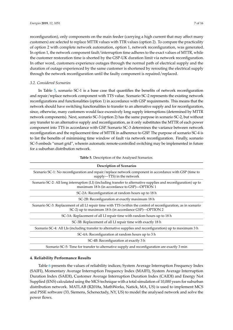
There are possibilities that the values for scenarios SC-2A and SC-2B, or SC-3A and SC-3B sharealmost similar values. In scenario SC-2A/3A, the time window of repair time/reconfiguration is bigger(up to 18 h), with multiple choices for selecting the hour for repair time or reconfiguration time. For asmaller window of reconfiguration/repair time, as in scenarios SC-4A (repair time up to 3 h) and SC-4B(repair time exactly 3 h), the values of CAIDI for both scenarios in Figure 4d were almost identical.

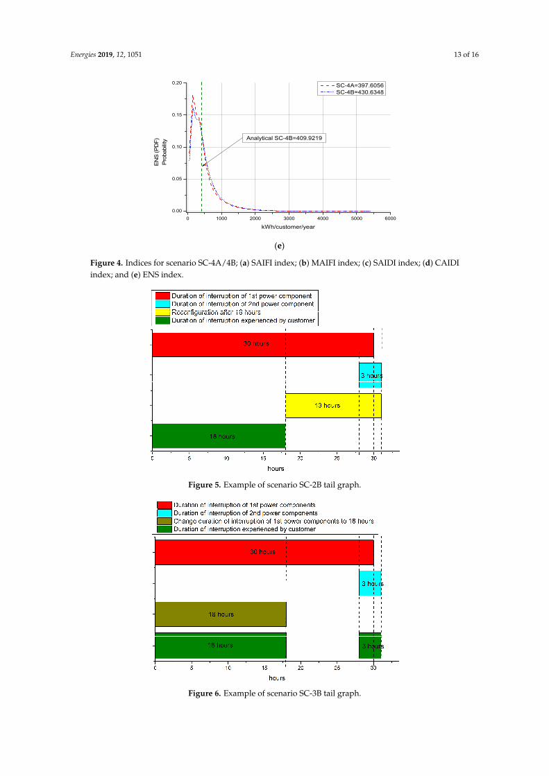
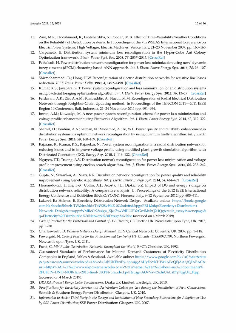
In Figure 3a, the MCS mean value of SAIFI scenario SC-2B was slightly lower than SC-3B becausein scenario SC-2B (see Figure 5), the frequency of interruptions was lower than that in scenario SC-3B(see Figure 6). In Figure 5, customers only experienced single interruption, while double interruptionsare shown in Figure 6. Thus, scenario SC-3B exhibited higher values of average duration of interruptionthan those recorded for scenario SC-2B.

Figures 5 and 6 portray the tail graphs of scenarios SC-2B and SC-3B for better understanding.In Figures 5 and 6, the same customers experienced LIs with varied average duration of interruption.In Figure 5, no second duration of interruption was noted, while in Figure 6, the customer experienceda second interruption within a 3 h duration. Thus, as displayed in Figure 6, the duration of interruptionwas 21 h, which is longer than that in Figure 5, 18 h.

As for scenario SC-5, when “smart grid” automatic switching was applied to the networkreconfiguration, the CAIDI values (i.e., average duration of LIs) increased after all faults were addressedwithin 18 h, to turn into Sis, due to less than 3 min of automatic switching. In detail, the shorterduration of LI no longer contributes to the average values, causing the average values of CAIDI ofscenario SC-5 to be higher. This also indicates that automatic switching reduced the number of LIs butincreased the average duration of interruptions and the number of SIs.

Energies 2019, 12, 1051 10 of 16

Energies 2019, 12, x FOR PEER REVIEW 9 of 16

ENS 346.5313

0 1 2 3 40.00

0.02

0.04

0.06

0.08

0.10

0.12

0.14

0.16

0.18

0.20

Analytical SC-5=0.1573S

AIFI

(PD

F)P

roba

bilit

y

long interruption/customer/year

MCS SC-1=0.4929 (mean) MCS SC-2A=0.4787 (mean) MCS SC-2B=0.4682 (mean) MCS SC-3A=0.4847 (mean) MCS SC-3B=0.4854 (mean) MCS SC-5=0.1514 (mean)

Analytical SC-1/SC-2A/SC-2B/SC-3A/SC-3B=0.4812

(a)

0 1 2 3 4 50.00

0.02

0.04

0.06

0.08

0.10

MAI

FI (P

DF)

Pro

babi

lity

short interruption/customer/year


Analytical SC-5=0.8887

Analytical SC-1/SC-2A/SC-2B/SC-3A/SC-3B=0.5649

(b)

0 100 200 300 400 500 6000.00

0.05

0.10

0.15

0.20

0.25


SAID

I (PD

F)P

roba

bilit

y

hours/customer/year



Analytical SC-2B/3B=8.3374

5 10 15 20 25 30 350.00

0.05

0.10

0.15

0.20

(c)

Figure 3. Cont.


0 100 200 300 400 5000.00

0.02

0.04

0.06

0.08

MCS SC-3B=190.5

MCS SC-2B=175.5



CAI

DI (

PDF)

Pro

babi

lity

hours/customer interruption



20 30 40 50 60 700.00

0.02

0.04

0.06

0.08

160 180 200-0.0001

0.0000

0.0001

0.0002

(d)

0 10000 20000 30000 40000 50000 600000.00

0.05

0.10

0.15

0.20

0.25



ENS

(PD

F)Pr

obab

ility

kWh/customer/year



500 1000 1500 2000 2500 3000 35000.00

0.05

0.10

0.15

0.20

(e)

Figure 3. Indices for scenario SC-1, SC-2A/2B, SC-3A/3B and SC-5. (a) SAIFI index; (b) MAIFI index; (c) SAIDI index; (d) CAIDI index; and (e) ENS index.

0.0 0.5 1.0 1.5 2.0 2.5 3.0 3.5 4.00.00

0.02

0.04

0.06

0.08

0.10

SAIF

I (P

DF)

Pro

babi

lity


MCS SC-4A=0.4733 (mean) MCS SC-4B=0.4734 (mean)


(a)

Figure 3. Indices for scenario SC-1, SC-2A/2B, SC-3A/3B and SC-5. (a) SAIFI index; (b) MAIFI index;(c) SAIDI index; (d) CAIDI index; and (e) ENS index.


0 100 200 300 400 5000.00

0.02

0.04

0.06

0.08

MCS SC-3B=190.5

MCS SC-2B=175.5



CAI

DI (

PDF)

Pro

babi

lity




20 30 40 50 60 700.00

0.02

0.04

0.06

0.08

160 180 200-0.0001

0.0000

0.0001

0.0002

(d)

0 10000 20000 30000 40000 50000 600000.00

0.05

0.10

0.15

0.20

0.25



ENS

(PD

F)Pr

obab

ility

kWh/customer/year



500 1000 1500 2000 2500 3000 35000.00

0.05

0.10

0.15

0.20

(e)

Figure 3. Indices for scenario SC-1, SC-2A/2B, SC-3A/3B and SC-5. (a) SAIFI index; (b) MAIFI index; (c) SAIDI index; (d) CAIDI index; and (e) ENS index.

0.0 0.5 1.0 1.5 2.0 2.5 3.0 3.5 4.00.00

0.02

0.04

0.06

0.08

0.10

SAIF

I (P

DF)

Pro

babi

lity




(a)

Figure 4. Cont.


0.0 0.5 1.0 1.5 2.0 2.5 3.0 3.5 4.00.00

0.02

0.04

0.06

0.08

0.10

MAI

FI (P

DF)

Prob

abili

ty

short interruption/customer/year



(b)

0 10 20 30 40 50 600.00

0.02

0.04

0.06

0.08

0.10

0.12

0.14

0.16

0.18

SAID

I (PD

F)Pr

obab

ility

hours/customer/year


Analytical SC-4B=4.1323

(c)

0 20 40 60 80 100 120 140 160 180 2000.00

0.02

0.04

0.06

0.08

CA

IDI (

PD

F)Pr

obab

ility




(d)

Figure 4. Cont.


0 1000 2000 3000 4000 5000 6000

0.00

0.05

0.10

0.15

0.20

ENS

(PD

F)P

roba

bilit

y

kWh/customer/year

SC-4A=397.6056 SC-4B=430.6348


(e)

Figure 4. Indices for scenario SC-4A/4B; (a) SAIFI index; (b) MAIFI index; (c) SAIDI index; (d) CAIDI index; and (e) ENS index.

5. Discussion

The results of scenarios SC-1, SC-2A/2B, and SC-3A/3B suggest that network reconfiguration and repair/replace with TTS can successfully reduce long supply interruptions. Figure 2d illustrates that the MCS outputs displayed a greater reduction in hours, from 68.4914 to 13.7321/18.1494, for scenarios SC-1 and SC-2B/3B, respectively.

In scenarios SC-2A/2B and SC-3A/3B, although the methods (options 1 and 2) of restoration supply differed, both scenarios shared almost similar values. In detail, Figure 2d shows that the line graph of scenario SC-2B is up to 175.5 h, while that for scenario SC-3B is up to 190.5 h. This signifies that for scenario SC-2B, two separate durations of interruptions occurred, and they overlapped with the reconfiguration duration time causing the tail of scenario SC-2B to be smaller than scenario SC-3B.

In Figure 3a, the MCS mean value of SAIFI scenario SC-2B was slightly lower than SC-3B because in scenario SC-2B (see Figure 5), the frequency of interruptions was lower than that in scenario SC-3B (see Figure 6). In Figure 5, customers only experienced single interruption, while double interruptions are shown in Figure 6. Thus, scenario SC-3B exhibited higher values of average duration of interruption than those recorded for scenario SC-2B.

Between scenarios SC-2A and SC-2B, or SC-3A and SC-3B, huge variances were noted in the values based on Figure 3d (CAIDI index). This is because the repair time in scenario SC-2B/3B was always exactly 18 h, while in scenario SC-2A/3A, although the repair time window was up to 18 h, it was not always exactly 18 h. This led the values of CAIDI in Figure 3d for scenario SC-2A/3A to be lower than scenario SC-2B/3B. As long as the duration of interruption is within the permissible limit (scenario SC-2A/3A), the values are acceptable.

There are possibilities that the values for scenarios SC-2A and SC-2B, or SC-3A and SC-3B share almost similar values. In scenario SC-2A/3A, the time window of repair time/reconfiguration is bigger (up to 18 h), with multiple choices for selecting the hour for repair time or reconfiguration time. For a smaller window of reconfiguration/repair time, as in scenarios SC-4A (repair time up to 3 h) and SC-4B (repair time exactly 3 h), the values of CAIDI for both scenarios in Figure 3d were almost identical.

Figures 5 and 6 portray the tail graphs of scenarios SC-2B and SC-3B for better understanding. In Figures 5 and 6, the same customers experienced LIs with varied average duration of interruption. In Figure 5, no second duration of interruption was noted, while in Figure 6, the customer experienced a second interruption within a 3 h duration. Thus, as displayed in Figure 6, the duration of interruption was 21 h, which is longer than that in Figure 5, 18 h.

Figure 4. Indices for scenario SC-4A/4B; (a) SAIFI index; (b) MAIFI index; (c) SAIDI index; (d) CAIDIindex; and (e) ENS index.


Figure 5. Example of scenario SC-2B tail graph.


As for scenario SC-5, when “smart grid” automatic switching was applied to the network reconfiguration, the CAIDI values (i.e., average duration of LIs) increased after all faults were addressed within 18 h, to turn into Sis, due to less than 3 min of automatic switching. In detail, the shorter duration of LI no longer contributes to the average values, causing the average values of CAIDI of scenario SC-5 to be higher. This also indicates that automatic switching reduced the number of LIs but increased the average duration of interruptions and the number of SIs.

6. Conclusions

This paper presents the reliability performance under various reconfigurations and replacement repair times based on regulator supply requirements. Each presented scenario has its own pros and cons. It is possible and realistic to change the mode of operation from a power loss-based to a regulator reliability-based network reconfiguration or repair/replace network component by adhering to GSP requirements on the existing network, so as to meet the target set by the energy regulator. In option 1 (network reconfiguration), the selection of restoration time (either 3 min, or 3 or 18 h) was unrestricted by human activity and weather, as DNOs may operate switches/breakers manually or automatically, rerouting the electrical supply. As for option 2 (repair/replace network





As for scenario SC-5, when “smart grid” automatic switching was applied to the network reconfiguration, the CAIDI values (i.e., average duration of LIs) increased after all faults were addressed within 18 h, to turn into Sis, due to less than 3 min of automatic switching. In detail, the shorter duration of LI no longer contributes to the average values, causing the average values of CAIDI of scenario SC-5 to be higher. This also indicates that automatic switching reduced the number of LIs but increased the average duration of interruptions and the number of SIs.

6. Conclusions

This paper presents the reliability performance under various reconfigurations and replacement repair times based on regulator supply requirements. Each presented scenario has its own pros and cons. It is possible and realistic to change the mode of operation from a power loss-based to a regulator reliability-based network reconfiguration or repair/replace network component by adhering to GSP requirements on the existing network, so as to meet the target set by the energy regulator. In option 1 (network reconfiguration), the selection of restoration time (either 3 min, or 3 or 18 h) was unrestricted by human activity and weather, as DNOs may operate switches/breakers manually or automatically, rerouting the electrical supply. As for option 2 (repair/replace network


Energies 2019, 12, 1051 14 of 16

6. Conclusions

This paper presents the reliability performance under various reconfigurations and replacementrepair times based on regulator supply requirements. Each presented scenario has its own prosand cons. It is possible and realistic to change the mode of operation from a power loss-based to aregulator reliability-based network reconfiguration or repair/replace network component by adheringto GSP requirements on the existing network, so as to meet the target set by the energy regulator.In option 1 (network reconfiguration), the selection of restoration time (either 3 min, or 3 or 18 h) wasunrestricted by human activity and weather, as DNOs may operate switches/breakers manually orautomatically, rerouting the electrical supply. As for option 2 (repair/replace network componentwith TTS value), it is practical to completely clear the fault within 18 h, but optional (either feasibleor otherwise) for 3 h or below 3 h. The 3 h replacement/repairing of network component dependson the definition, by including or excluding travelling time, locating fault area, weather condition,and others. Hence, several scenarios bring about extra flexibility to DNOs. DNOs may choose themost appropriate methods/options or scenario in accordance with their operation conditions and therequirements of the network system so as to meet their own reliability target, as well as the target fixedby the energy regulator.

Author Contributions: M.I.M.R. did the experiments and prepared the manuscript. S.Z.D guided the experimentsand paper writing.

Funding: Universiti Malaysia Pahang Internal Grant RDU1703260.

Acknowledgments: This research is supported by Universiti Malaysia Pahang Internal Grant RDU1703260.The authors would also like to thank the Faculty of Electrical & Electronics Engineering Universiti MalaysiaPahang and Institute for Energy System University of Edinburgh for providing facilities to conduct this researchand financial supports throughout the process.

Conflicts of Interest: The authors declare no conflict of interest.

References

1. The Electricity Standard of Performance Regulations Statutory Instruments. Standard No.698; Office of Gasand Electricity Markets (OFGEM): London, UK, 2010.

2. CEER. 6th CEER Benchmarking Report on the Quality of Electricity and Gas Supply 2016; Report Contin.Electricity Supply; CEER (Council of European Energy Regulators): Brussels, Belgium, 2016.

3. Engineering Recommendation P2/6 Security of Supply; Energy Networks Association (ENA): London, UK, 2005;pp. 1–13.

4. Liu, K.Y.; Sheng, W.; Liu, Y.; Meng, X. A network reconfiguration method considering data uncertainties insmart distribution networks. Energies 2017, 10, 618.

5. Wen, J.; Tan, Y.; Jiang, L. A reconfiguration strategy of distribution networks considering node importance.PLoS ONE 2016, 11, 1–20. [CrossRef] [PubMed]

6. Flaih, F.; Lin, X.; Abd, M.; Dawoud, S.; Li, Z.; Adio, O. A New Method for Distribution NetworkReconfiguration Analysis under Different Load Demands. Energies 2017, 10, 455. [CrossRef]

7. Nguyen, T.T.; Truong, A.V.; Phung, T.A. A novel method based on adaptive cuckoo search for optimalnetwork reconfiguration and distributed generation allocation in distribution network. Int. J. Electr.Power Energy Syst. 2016, 78, 801–815. [CrossRef]

8. Adoghe, A.U.; Awosope, C.O.A.; Ekeh, J.C. Asset maintenance planning in electric power distributionnetwork using statistical analysis of outage data. Int. J. Electr. Power Energy Syst. 2013, 47, 424–435.[CrossRef]

9. Vale, Z.; Soares, J.; Lobo, C.; Canizes, B. Multi-criteria optimisation approach to increase the delivered powerin radial distribution networks. IET Gener. Transm. Distrib. 2015, 9, 2565–2574.

10. Usberti, F.L.; Lyra, C.; Cavellucci, C.; González, J.F.V. Hierarchical multiple criteria optimization ofmaintenance activities on power distribution networks. Ann. Oper. Res. 2015, 224, 171–192. [CrossRef]

http://dx.doi.org/10.1371/journal.pone.0168350

http://www.ncbi.nlm.nih.gov/pubmed/27992589

http://dx.doi.org/10.3390/en10040455

http://dx.doi.org/10.1016/j.ijepes.2015.12.030


http://dx.doi.org/10.1007/s10479-012-1182-6

Energies 2019, 12, 1051 15 of 16

11. Zare, M.R.; Hooshmand, R.; Eshtehardiha, S.; Poodeh, M.B. Effect of Time-Variability Weather Conditionson the Reliability of Distribution Systems. In Proceedings of the 7th WSEAS International Conference onElectric Power Systems, High Voltages, Electric Machines, Venice, Italy, 21–23 November 2007; pp. 160–165.

12. Carpaneto, E. Distribution system minimum loss reconfiguration in the Hyper-Cube Ant ColonyOptimization framework. Electr. Power Syst. Res. 2008, 78, 2037–2045. [CrossRef]

13. Fathabadi, H. Power distribution network reconfiguration for power loss minimization using novel dynamicfuzzy c-means (dFCM) clustering based ANN approach. Int. J. Electr. Power Energy Syst. 2016, 78, 96–107.[CrossRef]

14. Shirmohammadi, D.; Hong, H.W. Reconfiguration of electric distribution networks for resistive line lossesreduction. IEEE Trans. Power Deliv. 1989, 4, 1492–1498. [CrossRef]

15. Kumar, K.S.; Jayabarathi, T. Power system reconfiguration and loss minimization for an distribution systemsusing bacterial foraging optimization algorithm. Int. J. Electr. Power Energy Syst. 2012, 36, 13–17. [CrossRef]

16. Ferdavani, A.K.; Zin, A.A.M.; Khairuddin, A.; Naeini, M.M. Reconfiguration of Radial Electrical DistributionNetwork through Neighbor-Chain Updating method. In Proceedings of the TENCON 2011—2011 IEEERegion 10 Conference, Bali, Indonesia, 21–24 November 2011; pp. 991–994.

17. Imran, A.M.; Kowsalya, M. A new power system reconfiguration scheme for power loss minimization andvoltage profile enhancement using Fireworks Algorithm. Int. J. Electr. Power Energy Syst. 2014, 62, 312–322.[CrossRef]

18. Shareef, H.; Ibrahim, A.A.; Salman, N.; Mohamed, A.; Ai, W.L. Power quality and reliability enhancement indistribution systems via optimum network reconfiguration by using quantum firefly algorithm. Int. J. Electr.Power Energy Syst. 2014, 58, 160–169. [CrossRef]

19. Rajaram, R.; Kumar, K.S.; Rajasekar, N. Power system reconfiguration in a radial distribution network forreducing losses and to improve voltage profile using modified plant growth simulation algorithm withDistributed Generation (DG). Energy Rep. 2015, 1, 116–122. [CrossRef]

20. Nguyen, T.T.; Truong, A.V. Distribution network reconfiguration for power loss minimization and voltageprofile improvement using cuckoo search algorithm. Int. J. Electr. Power Energy Syst. 2015, 68, 233–242.[CrossRef]

21. Gupta, N.; Swarnkar, A.; Niazi, K.R. Distribution network reconfiguration for power quality and reliabilityimprovement using Genetic Algorithms. Int. J. Electr. Power Energy Syst. 2014, 54, 664–671. [CrossRef]

22. Hernando-Gil, I.; Ilie, I.-S.; Collin, A.J.; Acosta, J.L.; Djokic, S.Z. Impact of DG and energy storage ondistribution network reliability: A comparative analysis. In Proceedings of the 2012 IEEE InternationalEnergy Conference and Exhibition (ENERGYCON), Florence, Italy, 9–12 September 2012; pp. 605–611.

23. Lakervi, E.; Holmes, E. Electricity Distribution Network Design. Available online: https://books.google.com.hk/books?hl=zh-TW&lr=&id=TpW28vHkE-0C&oi=fnd&pg=PR11&dq=Electricity+Distribution+Network+Design&ots=ppzWMReCr2&sig=_Kjze7swVrRLUPYoGwiMubQX4Qg&redir_esc=y#v=onepage&q=Electricity%20Distribution%20Network%20Design&f=false (accessed on 4 March 2019).

24. Code of Practice for the Protection and Control of HV Circuits; CE Electric UK: Newcastle upon Tyne, UK, 2015;pp. 1–30.

25. Charlesworth, D. Primary Network Design Manual; EON Central Network: Coventry, UK, 2007; pp. 1–118.26. Powergrid, N. Code of Practice for the Protection and Control of HV Circuits (DSS/007/010); Northern Powergrid:

Newcastle upon Tyne, UK, 2011.27. Puret, C. MV Public Distribution Networks throughout the World; E/CT: Cheshire, UK, 1992.28. Guaranteed Standards of Performance for Metered Demand Customers of Electricity Distribution

Companies in England, Wales & Scotland. Available online: https://www.google.com.hk/url?sa=t&rct=j&q=&esrc=s&source=web&cd=1&ved=2ahUKEwiEy-6phujgAhUyE6YKHWr7AFoQFjAAegQIABAC&url=https%3A%2F%2Fwww.ukpowernetworks.co.uk%2Finternet%2Fen%2Fabout-us%2Fdocuments%2FUKPN-DNO-NOR-Jan-2013-final-UKPN-branded.pdf&usg=AOvVaw24dnU4UsB7pt8jgUx_Fqrp(accessed on 4 March 2019).

29. DRAKA Product Range Cable Specifications; Draka UK Limited: Eastleigh, UK, 2010.30. Specifications for Electricity Service and Distribution Cables for Use during the Installation of New Connections;

Scottish & Southern Energy Power Distribution: Glasgow, UK, 2010.31. Information to Assist Third Party in the Design and Installation of New Secondary Substations for Adoption or Use

by SSE Power Distribution; SSE Power Distribution: Glasgow, UK, 2007.

http://dx.doi.org/10.1016/j.epsr.2008.06.009


http://dx.doi.org/10.1109/61.25637




http://dx.doi.org/10.1016/j.egyr.2015.03.002



https://books.google.com.hk/books?hl=zh-TW&lr=&id=TpW28vHkE-0C&oi=fnd&pg=PR11&dq=Electricity+Distribution+Network+Design&ots=ppzWMReCr2&sig=_Kjze7swVrRLUPYoGwiMubQX4Qg&redir_esc=y#v=onepage&q=Electricity%20Distribution%20Network%20Design&f=false




https://www.google.com.hk/url?sa=t&rct=j&q=&esrc=s&source=web&cd=1&ved=2ahUKEwiEy-6phujgAhUyE6YKHWr7AFoQFjAAegQIABAC&url=https%3A%2F%2Fwww.ukpowernetworks.co.uk%2Finternet%2Fen%2Fabout-us%2Fdocuments%2FUKPN-DNO-NOR-Jan-2013-final-UKPN-branded.pdf&usg=AOvVaw24dnU4UsB7pt8jgUx_Fqrp




Energies 2019, 12, 1051 16 of 16

32. Distribution Long Term Development Statement for the Years 2011/12 to 2015/16; SP Distribution and SP Manweb:Glasgow, UK, 2011.

33. National System and Equipment Performance Report; Energy Networks Association (ENA): London, UK, 2010.34. Allan, R.; de Oliveira, M. Evaluating the reliability of electrical auxiliary systems in multi-unit generating

stations. IEE Proc. C Gener. Transm. Distrib. 1980, 127, 65–71. [CrossRef]35. Stanek, E.; Venkata, S. Mine power system reliability. IEEE Trans. Ind. Appl. 1988, 24, 827–838. [CrossRef]36. Farag, A.; Wang, C.; Cheng, T. Failure analysis of composite dielectric of power capacitors in distribution

systems. Electr. Power Syst. Res. 1998, 44, 117–126. [CrossRef]37. Office of Gas and Electricity Markets. The Performance of Networks Using Alternative Splitting Configurations;

Final Report on Technical Steering Group Workstream; Office of Gas and Electricity Markets (OFGEM):London, UK, 2004.

38. Roos, F.; Lindah, S. Distribution system component failure rates and repair times—An overview. In Proceedingsof the Nordic Distribution and Asset Management Conference, Espoo, Finland, 23–24 August 2004.

39. Anders, G.; Maciejewski, H. A comprehensive study of outage rates of air blast breakers. IEEE Trans.Power Syst. 2006, 21, 202–210. [CrossRef]

40. Office of Gas and Electricity Markets. Review of Electricity Transmission Output Measures; Final Report;Office of Gas and Electricity Markets (OFGEM): London, UK, 2008.

41. He, Y. Study and Analysis of Distribution Equipment Reliability Data; Elforsk AB: Stockholm, Sweden, 2010.42. Office of Gas and Electricity Markets (OFGEM). Electricity Distribution Quality of Service Report 2008/09; Office

of Gas and Electricity Markets: London, UK, 2009.43. Billinton, R.; Allan, R. Reliability Evaluation of Power Systems, 2nd ed.; Springer: New York, NY, USA, 1996.44. Bie, Z.; Zhang, P.; Li, G.; Hua, B.; Meehan, M.; Wang, X. Reliability Evaluation of Active Distribution Systems

Including Microgrids. IEEE Trans. Power Syst. 2012, 27, 2342–2350. [CrossRef]45. Arya, L.D.; Choube, S.C.; Arya, R.; Tiwary, A. Evaluation of reliability indices accounting omission of random

repair time for distribution systems using Monte Carlo simulation. Int. J. Electr. Power Energy Syst. 2012, 42,533–541. [CrossRef]

46. Zhang, H.; Li, P. Probabilistic analysis for optimal power flow under uncertainty. IET Gener. Transm. Distrib.2010, 4, 553. [CrossRef]

47. Alvehag, K.; Söder, L. Risk-based method for distribution system reliability investment decisions underperformance-based regulation. IET Gener. Transm. Distrib. 2011, 5, 1062. [CrossRef]

48. Hadjsaid, N.; Sabonnadiere, J.-C. Electrical Distribution Networks; John Wiley & Sons: Hoboken, NJ, USA, 2013.49. Hribar, L.; Duka, D. Weibull distribution in modeling component faults. In Proceedings of the ELMAR-2010,

Zadar, Croatia, 15–17 September 2010; pp. 183–186.50. Rubinstein, R.Y.; Kroese, D.P. Simulation and the Monte Carlo Method; John Wiley & Sons, Inc.: Hoboken, NJ,

USA, 2016.

© 2019 by the authors. Licensee MDPI, Basel, Switzerland. This article is an open accessarticle distributed under the terms and conditions of the Creative Commons Attribution(CC BY) license (http://creativecommons.org/licenses/by/4.0/).

http://dx.doi.org/10.1049/ip-c.1980.0011

http://dx.doi.org/10.1109/28.8987

http://dx.doi.org/10.1016/S0378-7796(97)01191-7

http://dx.doi.org/10.1109/TPWRS.2005.860941

http://dx.doi.org/10.1109/TPWRS.2012.2202695


http://dx.doi.org/10.1049/iet-gtd.2009.0374

http://dx.doi.org/10.1049/iet-gtd.2011.0047

http://creativecommons.org/

http://creativecommons.org/licenses/by/4.0/.

energy regulator supply restoration time

Documents