Energy Savings and Collateral Impacts of a DHW Water-to-Water Heat Pump System withSubslab Earth Coupling

William D. Rittelmann, PEMember ASHRAE

ABSTRACT

This paper presents research results from simulations and a field investigation of a domestic hot water (DHW) system incor-porating a water-to-water heat pump and a subslab earth-coupled loop. The research stems from a need for nonsolar, high-effi-ciency, DHW system alternatives to help reach the whole-house energy savings goals of 50% and higher. A schematic diagramof the system is used to explain the system concept, emphasizing daily average DHW loads and the resulting load density imposedon the slab. A comparison to air-to-water heat pumps summarizes the primary advantages and market barriers of this systemtype. A summary of the analysis using a transient system simulation model is reviewed, and sensitivity to key system parametersand user schedules is discussed. The relative importance of subhourly simulation time steps and hot water demand schedules isexplained. Collateral energy impacts of individual system components are then presented on monthly and annual bases andcompared to results from a base-case simulation incorporating a conventional electric resistance water heater. Additional orreduced heat flux through the slab and standby tank losses/gains are of particular interest, as are variations due to foundationtype and climate. The calculation of the net whole-house coefficient of performance is explained and total annual energy consump-tion is presented.

INTRODUCTION

Domestic hot water (DHW) energy use accounts for anaverage of 17% of all residential site energy use in a typicalsingle-family home (EIA 2001). This percentage can be ashigh as 40% in an energy-efficient home as the energy effi-ciency of the building envelope and space-conditioningsystem increases. Current federal minimum energy factors forwater heaters (DOE 2001) are 0.59 for a typical 40-gallon gas-fired tank-type water heater and 0.90 for a 50-gallon electricwater heater. Maximum energy factors (GAMA 2007) are0.85 for gas-fired water heaters and 2.28 for air-to-water heatpump water heaters (HPWHs).

Although it may appear possible to attain large energysavings by using an HPWH, there are two other factors onemust consider. Current Building America goals (NREL 2007)target source energy savings. Applying national average site-to-source energy multipliers, the best gas-fired water heater

still has a source-energy factor of 0.83, and an HPWH dropsto only 0.72. The second factor that is not normally consid-ered in the calculation of the energy factor is the net energyimpact on the space-conditioning system. Most water heatersonly add a small amount of heat to the space, but an HPWHremoves about as much thermal energy from the space aselectrical energy it consumes. For example, an air-to-waterHPWH operating in a space heated by an air-to-air heat pumpwith a heating seasonal performance factor (HSPF) of 9.90has a net source-energy factor of 0.51 during the heatingseason. On the other hand, heat removed from the spaceduring the cooling season increases the net source-energyfactor to 0.94. These interactions tend to decrease the net effi-ciency of HPWHs in heating-dominated climates andincrease it in cooling-dominated climates. A more noticeableeffect of these interactions is the cooler space temperaturesurrounding the HPWH year round.

© 2007 ASHRAE.

William D. Rittelmann is a senior research project manager for IBACOS, Inc., Pittsburgh, PA.

This research focuses on a water heating system thatincorporates a water-to-water heat pump system with a source/sink exterior to the conditioned space of the house whilerequiring minimum additional excavation. The target applica-tions are projects in climates or situations in which solar DHWsystems would not be practical or economically feasible.Preliminary system cost estimates, based on retail costs ofcommercially available air-to-water HPWHs and piping costs,put the installed cost of a mature, market-ready, water-to-water heat pump system at approximately $2,500. Althoughthis is several hundred dollars more than the installed cost ofa high-efficiency, tankless, gas-fired water heater, it is lessthan many solar DHW systems (Burch and Salasovich 2005).

EXPERIMENTAL DESIGN

Evaluation of the system shown in Figure 1 began withcomputer simulations using TRNSYS (TESS 2006b) to deter-mine the net annual energy efficiency of a water-to-waterHPWH and the impact of such a system on subslab earthtemperatures. Simulations were conducted for both warm andcold climates and two foundation types: slab-on-grade and fullbasement. Simulation results from the prototype system werethen compared to simulation results from similar systems,with the primary difference being that the earth-coupledpiping loop was modeled remotely from the building.

Results from the simulations were then used to design andconstruct a prototype system for field testing. Measured datawere then compared to simulation results to determine the sensi-tivity of the simulation output to various system parameters.

System Description for Simulations

A water-to-water heat pump extracts heat from under aninsulated slab to heat water via the integral heat exchanger inthe hot water tank. Components shown in Figure 1 aredescribed in the following paragraphs.

Hot Water Tank. The hot water tank is a solar-ready,300-liter (80-gallon) storage tank with a 4,500 W heatingelement in the upper part of the tank and an integral heatexchanger in the lower part. The tank is modeled in TRNSYS

as a stratified storage tank using Type 534 (TESS 2000). Forsimulation purposes, the tank volume is divided into eightvertical nodes and the heat exchanger is divided into fournodes equally distributed within the bottom half of the tank.The auxiliary heating element setpoint temperature is 50.0°C(122°F) with a deadband of 10.0°C (18.0°F). To minimizeenergy use of the auxiliary heating element, it is important thatthe setpoint temperature be equal to or lower than the heatpump setpoint temperature and that the temperature deadbandbe larger.

The integral heat exchanger consists of a 40 m (131 ft)coiled-copper pipe with an inside diameter of 16 mm (0.625 in.).

Heat Pump. The heat pump is a water-to-water heatpump with a nominal output capacity of 5.3 kW (1.5 ton)designed for DHW service. Catalogued performance data inFigures 2 and 3 illustrate the range in efficiency and capacitywith respect to inlet load and source water temperatures. Theellipses in each figure identify the region of operation for thesystem. The fluid in the source piping loop is pure water andthe fluid in the load loop is 50% propylene glycol and 50%water. The heat pump is controlled by an aquastat with asetpoint temperature of 50.0°C (122°F) and a deadband of5.0°C (9.0°F) located in the bottom of the hot water storage

Figure 1 System schematic.

Figure 2 Heat pump efficiency.

Figure 3 Heat pump capacity.

2 Buildings X

tank. A freeze stat prevents operation of the compressor whenthe source outlet temperature is below 1.7°C (35°F). The heatpump is simulated using TRNSYS Type 668 (TESS 2001).

Earth-Coupled Piping Loops. The subslab piping loopwas modeled as a single-circuit serpentine of PEX piping in a0.2 m (7.9 in.) thick sand bed under the insulated slab. Figure 4shows the layout and Table 1 lists the parameter values used inthe simulations.

Identical piping parameters were used when simulatingearth-coupled loops that are remote from the slab for compar-ison purposes. In these cases, TRNSYS Type 952 (TESS2006a) was used to model the buried pipe in two horizontalcircuits 2 m (6.6 ft) below the surface. In the Type 952 model,the piping is assumed to be spaced far enough apart to disre-gard interactions between parallel pipe sections. Far-fieldground temperatures are based on the Kusuda correlation

(Kusuda and Achenbach 1965) so that long-term temperaturechanges due to the heat flux into the pipe are not considered.

Foundations. The system was simulated using twodifferent foundation conditions: slab-on-grade and full base-ment. For both simulations, TRNSYS Type 706 (TESS 2003)was used. This component is intended to model a radiant floor-heating slab embedded in soil and containing a number offluid-filled pipes. The heat transfer within the slab andsurrounding soil is assumed to be conductive only, and mois-ture effects are not accounted for in the model. The modelrelies on a three-dimensional finite difference method, solvingthe resulting interdependent differential equations using aniterative approach. Slab nodes are defined by the user in eachgeometric plane and extend beyond the slab in all directionsexcept above. The floor that was modeled in both cases was a0.10 m (3.9 in.) concrete slab over 0.51 m (2 in.) of rigid insu-lation with a thermal resistance of 0.49 h·m2·K/kJ (10 h·ft2·°F/Btu). In the slab-on-grade case, vertical insulation alsoextends to a depth of 0.7 m (28 in.) into the ground around theperimeter of the slab. For these simulations, radiant heat trans-fer at the earth’s surface was included in the slab-on-grade casebut not in the full basement model. Soil temperatures at theslab plane in the full basement model were described using theKusuda correlation (Kusuda and Achenbach 1965) and thesoil and ground temperature properties are listed in Tables 2and 3. The Kusuda correlation was also used to describe theearth surface temperature of the slab-on-grade model becausethe energy balance surface mode does not consider evapora-tion, partial shading due to grass, and seasonal changes inground reflectance due to snow.

DHW Temperature and Usage Schedule. Hot waterevents were described as discrete fixture flow rates andtemperatures rather than specific hot water volumes to accountfor variations in flow due to seasonal variations in mains watertemperature and instantaneous variations in hot water temper-atures due to nonuniform temperatures in the storage tank.Parameter values for each event are shown in Table 4. Figure 4 Subslab piping layout.

Table 1. Earth-Coupled Piping Parameters

Pipe total length 150 m (492 ft)

Pipe inside diameter 13 mm (0.51 in.)

Pipe outside diameter 15 mm (0.59 in.)

Pipe material thermal conductivity 1.661 kJ/h·m·K (0.266 Btu/h·ft·°R)

Pipe material density 200 kg/m3 (12.5 lb/ft3)

Pipe/earth contact resistance 0.0001 h·m·K/kJ (0.002044 h·ft·°R/Btu)

Fluid thermal conductivity 2.066 kJ/h·m·K (0.332 Btu/h·ft·°R)

Fluid density 1000 kg/m3 (62.4 lb/ft3)

Fluid specific heat 4.19 kJ/kg·K (1.00 Btu/lb·°R)

Fluid viscosity 5.468 kg/m·h (3.228 lb·s/ft2)

Buildings X 3

SIMULATIONS

Simulations where performed for two cities, Chicago andMiami, and two foundation types, slab-on-grade and full base-ment. Due to the impact of the system on long-term groundtemperatures, each simulation was run for a period of fiveyears, and the results are shown for the last 12 months. A simu-lation time step of 7.5 min was used so as not to exceed theduration of the shortest hot water event. This is necessary tomaintain acceptable hot water delivery temperatures, whichwould not be possible using a time step of one hour.

SIMULATION RESULTS

Results were calculated on a monthly basis. Severaldifferent coefficients of performance (COPs) are shown sothat performance can be compared to the heat pump manufac-turer’s data, efficiencies of other water heating systems, andthe whole-house or integrated efficiency.

Heat Pump COP. The heat pump COP represents theheat pump energy output divided by the energy input of thecompressor.

System COP. The system COP is calculated by dividingthe DHW-delivered energy by the sum of the energy input ofthe compressor, circulating pumps, and auxiliary electric heat-ing element.

Integrated COP. The calculation of the integrated COPgoes two steps further than the system COP and includes theheat gain to the space from the storage tank and the net heatloss/gain through the floor slab. To determine these values, thesame model was run without the heat pump to benchmark

monthly heat losses through the floor slab. For heating seasonmonths, heat gains to the space caused by the DHW system areconsidered part of the output energy of the DHW system. Forthe cooling season, heat gains/losses to the space are dividedby the COP of an efficient space-conditioning system (5.57)and that value is then added to the energy input sum of theDHW system.

Sensible and latent loads from hot-water end uses, such asshowers and baths, were not simulated and, therefore, were notincluded in this COP due to the unknown and complex inter-actions of these loads with bathroom exhaust fans.

Cold Climate (Chicago)

Simulation results indicate that the proposed conceptprovides energy efficiency levels that are equal to or betterthan a conventional system in which the earth coupling isremote from the foundation of the house. Analysis performedusing Chicago weather data indicates that the annual averageintegrated COP is approximately 2.0 for both slab-on-gradeand full basement foundation application types (Figure 5),whereas a similar system with a remote earth-coupling (alsoFigure 5) yielded an annual COP of 1.7 to 2.1. (The remotesystem was modeled in two different ways, which arediscussed later in the paper.) A comparison of the system COPand the integrated COP of the prototype system illustrates thenegative effect of the additional heat loss through the slabduring the heating months and the beneficial effect in thesummer months. The same comparison of the remote systemillustrates the opposite effect due to the lack of any additional

Table 2. Ground Temperature Properties

ClimateMean Surface Temperature,

°C (°F)Surface Amplitude Temperature,

°C (°F)Shift,Days

Cold (Chicago, IL) 9.8 (49.1) 14.1 (25.7) 15

Warm (Miami, FL) 24.8 (76.7) 4.3 (7.8) 21

Table 3. Slab and Soil Properties

MaterialDensity,

kg/m3 (lb/ft3)Conductivity,

kJ/h·m·K (Btu/h·ft·°R)Specific Heat,

kJ/kg·K (Btu/lb·°R)

Slab 2400 (150) 2.15 (0.345) 0.90 (0.215)

Soil 2091 (131) 1.50 (1.10) 0.84 (0.201)

Table 4. DHW Event Temperature and Schedule

Event Event TypeFlow Rate,L/m (gpm)

Duration,min

Temperature,°C (°F)

StartTime

ShowerTemperaturedependent

9.5 (2.5) 7.5 40.0 (104)7:00 a.m., 7:30 a.m.,7:00 p.m., 7:30 p.m.

LaundryTemperatureindependent

9.5 (2.5) 7.5 Varies* 11:00 a.m.

* Equals instantaneous temperature of storage tank outlet.

4 Buildings X

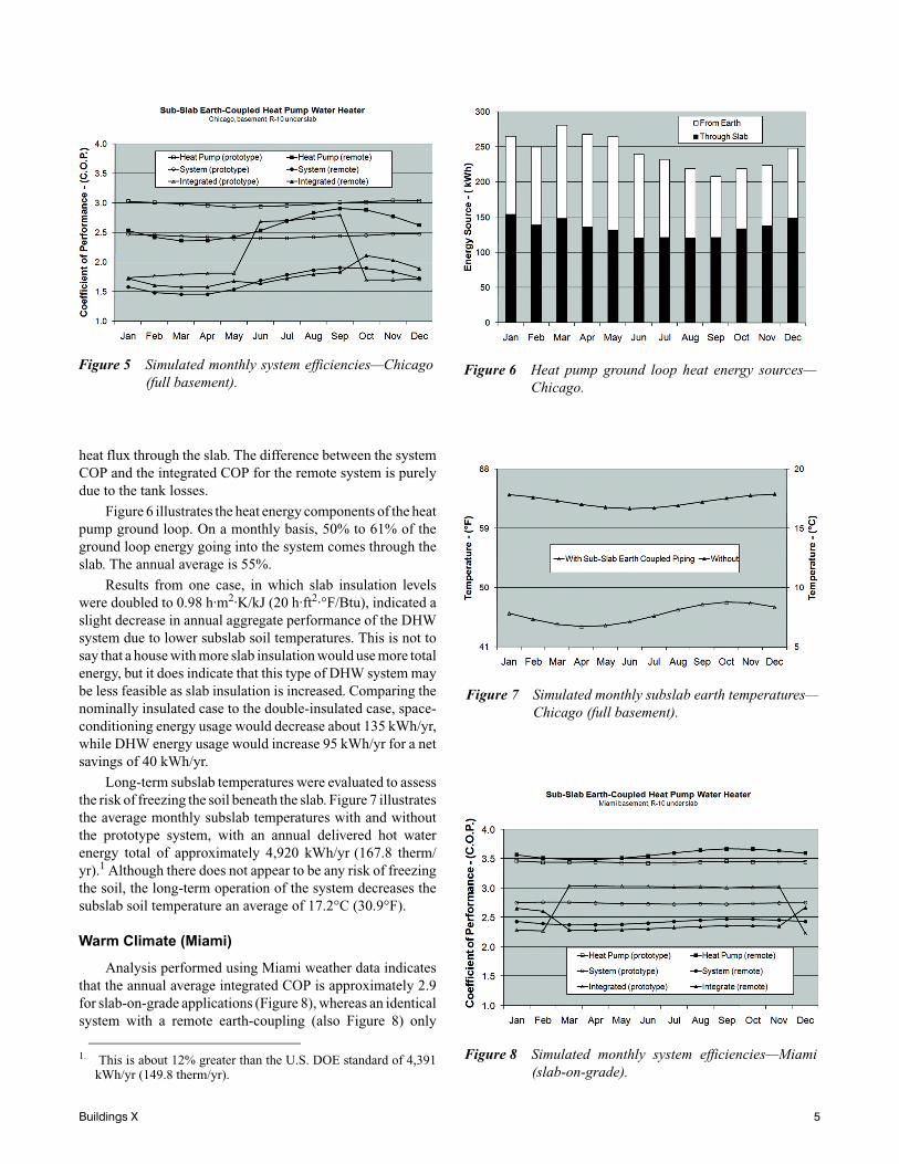
heat flux through the slab. The difference between the systemCOP and the integrated COP for the remote system is purelydue to the tank losses.

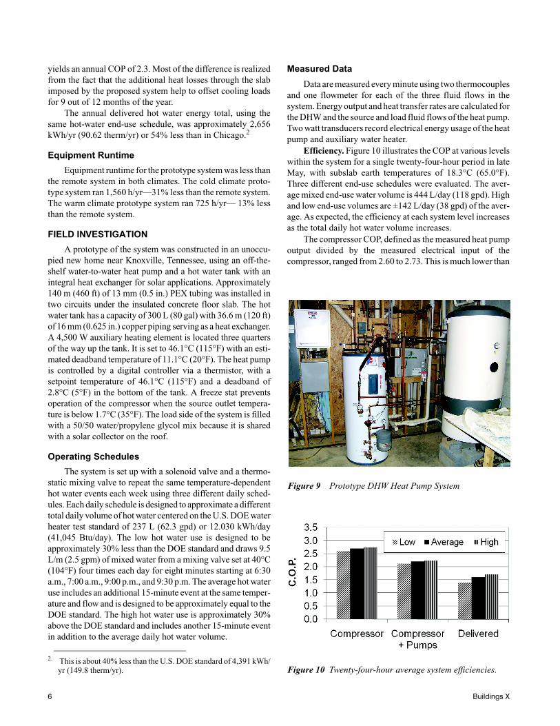
Figure 6 illustrates the heat energy components of the heatpump ground loop. On a monthly basis, 50% to 61% of theground loop energy going into the system comes through theslab. The annual average is 55%.

Results from one case, in which slab insulation levelswere doubled to 0.98 h·m2·K/kJ (20 h·ft2·°F/Btu), indicated aslight decrease in annual aggregate performance of the DHWsystem due to lower subslab soil temperatures. This is not tosay that a house with more slab insulation would use more totalenergy, but it does indicate that this type of DHW system maybe less feasible as slab insulation is increased. Comparing thenominally insulated case to the double-insulated case, space-conditioning energy usage would decrease about 135 kWh/yr,while DHW energy usage would increase 95 kWh/yr for a netsavings of 40 kWh/yr.

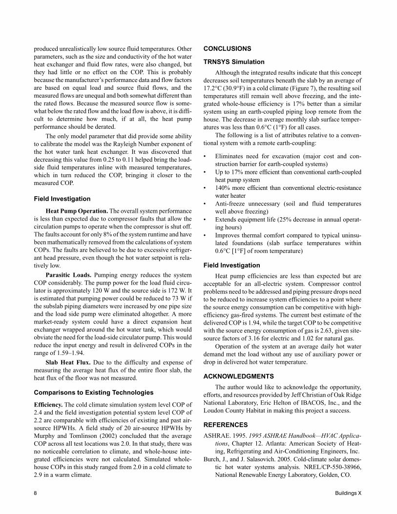
Long-term subslab temperatures were evaluated to assessthe risk of freezing the soil beneath the slab. Figure 7 illustratesthe average monthly subslab temperatures with and withoutthe prototype system, with an annual delivered hot waterenergy total of approximately 4,920 kWh/yr (167.8 therm/yr).1 Although there does not appear to be any risk of freezingthe soil, the long-term operation of the system decreases thesubslab soil temperature an average of 17.2°C (30.9°F).

Warm Climate (Miami)

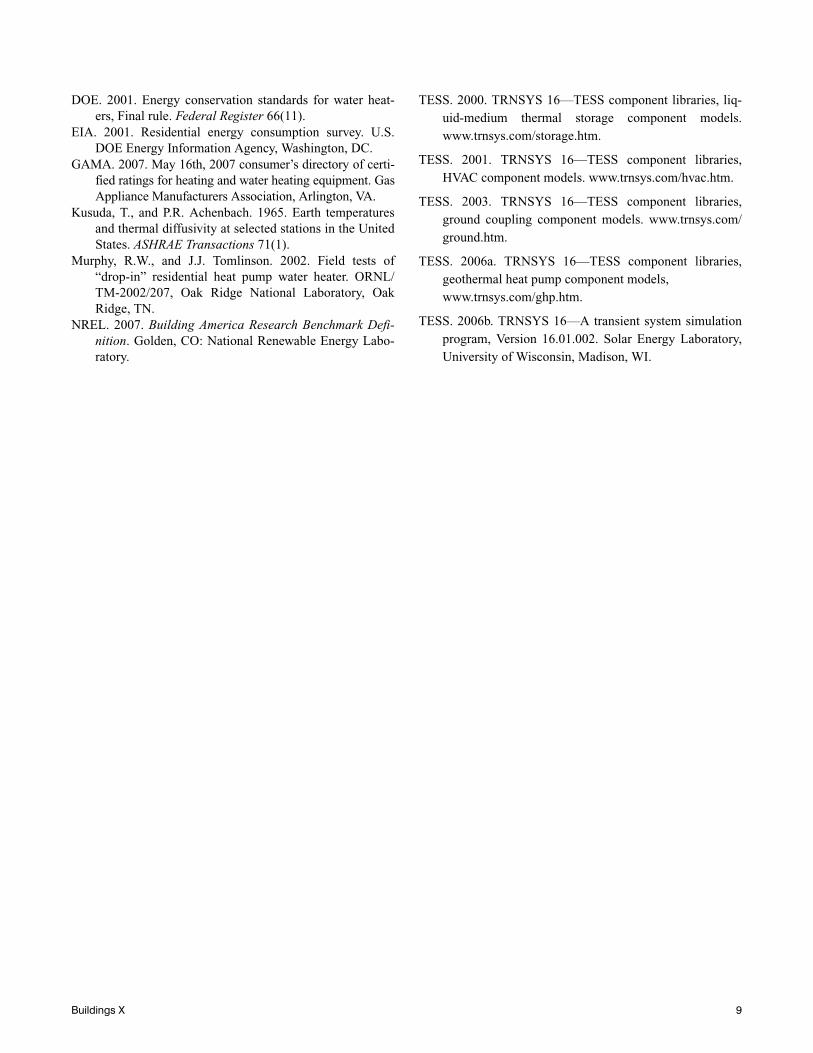
Analysis performed using Miami weather data indicatesthat the annual average integrated COP is approximately 2.9for slab-on-grade applications (Figure 8), whereas an identicalsystem with a remote earth-coupling (also Figure 8) only

1. This is about 12% greater than the U.S. DOE standard of 4,391kWh/yr (149.8 therm/yr).

Figure 5 Simulated monthly system efficiencies—Chicago(full basement).

Figure 6 Heat pump ground loop heat energy sources—Chicago.

Figure 7 Simulated monthly subslab earth temperatures—Chicago (full basement).

Figure 8 Simulated monthly system efficiencies—Miami(slab-on-grade).

Buildings X 5

yields an annual COP of 2.3. Most of the difference is realizedfrom the fact that the additional heat losses through the slabimposed by the proposed system help to offset cooling loadsfor 9 out of 12 months of the year.

The annual delivered hot water energy total, using thesame hot-water end-use schedule, was approximately 2,656kWh/yr (90.62 therm/yr) or 54% less than in Chicago.2

Equipment Runtime

Equipment runtime for the prototype system was less thanthe remote system in both climates. The cold climate proto-type system ran 1,560 h/yr—31% less than the remote system.The warm climate prototype system ran 725 h/yr— 13% lessthan the remote system.

FIELD INVESTIGATION

A prototype of the system was constructed in an unoccu-pied new home near Knoxville, Tennessee, using an off-the-shelf water-to-water heat pump and a hot water tank with anintegral heat exchanger for solar applications. Approximately140 m (460 ft) of 13 mm (0.5 in.) PEX tubing was installed intwo circuits under the insulated concrete floor slab. The hotwater tank has a capacity of 300 L (80 gal) with 36.6 m (120 ft)of 16 mm (0.625 in.) copper piping serving as a heat exchanger.A 4,500 W auxiliary heating element is located three quartersof the way up the tank. It is set to 46.1°C (115°F) with an esti-mated deadband temperature of 11.1°C (20°F). The heat pumpis controlled by a digital controller via a thermistor, with asetpoint temperature of 46.1°C (115°F) and a deadband of2.8°C (5°F) in the bottom of the tank. A freeze stat preventsoperation of the compressor when the source outlet tempera-ture is below 1.7°C (35°F). The load side of the system is filledwith a 50/50 water/propylene glycol mix because it is sharedwith a solar collector on the roof.

Operating Schedules

The system is set up with a solenoid valve and a thermo-static mixing valve to repeat the same temperature-dependenthot water events each week using three different daily sched-ules. Each daily schedule is designed to approximate a differenttotal daily volume of hot water centered on the U.S. DOE waterheater test standard of 237 L (62.3 gpd) or 12.030 kWh/day(41,045 Btu/day). The low hot water use is designed to beapproximately 30% less than the DOE standard and draws 9.5L/m (2.5 gpm) of mixed water from a mixing valve set at 40°C(104°F) four times each day for eight minutes starting at 6:30a.m., 7:00 a.m., 9:00 p.m., and 9:30 p.m. The average hot wateruse includes an additional 15-minute event at the same temper-ature and flow and is designed to be approximately equal to theDOE standard. The high hot water use is approximately 30%above the DOE standard and includes another 15-minute eventin addition to the average daily hot water volume.

Measured Data

Data are measured every minute using two thermocouplesand one flowmeter for each of the three fluid flows in thesystem. Energy output and heat transfer rates are calculated forthe DHW and the source and load fluid flows of the heat pump.Two watt transducers record electrical energy usage of the heatpump and auxiliary water heater.

Efficiency. Figure 10 illustrates the COP at various levelswithin the system for a single twenty-four-hour period in lateMay, with subslab earth temperatures of 18.3°C (65.0°F).Three different end-use schedules were evaluated. The aver-age mixed end-use water volume is 444 L/day (118 gpd). Highand low end-use volumes are ±142 L/day (38 gpd) of the aver-age. As expected, the efficiency at each system level increasesas the total daily hot water volume increases.

The compressor COP, defined as the measured heat pumpoutput divided by the measured electrical input of thecompressor, ranged from 2.60 to 2.73. This is much lower than

2. This is about 40% less than the U.S. DOE standard of 4,391 kWh/yr (149.8 therm/yr).

Figure 9 Prototype DHW Heat Pump System

Figure 10 Twenty-four-hour average system efficiencies.

6 Buildings X

the simulated performance for similar ground temperatures,which yielded a COP of 3.33.

The COP of the compressor plus the pumps includes theelectrical input of the circulator pumps in the denominator, inaddition to the compressor, and ranges from 1.98 to 2.01. Thisefficiency is somewhat lower than expected due to short-cycling of the compressor, which allowed the circulator pumpsto run more than the compressor. Calculation of this COP,using only the pumping energy that is coincident with thecompressor energy, yields a COP range of 2.12–2.23, which isthe value shown in the chart.

The delivered COP is calculated as the net delivered DHWenergy divided by the electrical input of the compressor,pumps, and auxiliary water heater. Again, the performance wasworse than expected due to the added runtime of the circulatingpumps because of the short cycling of the heat pump. Correct-ing for the short cycling problem increases the COP range to1.39–1.70, which are the values shown in the chart.

Figure 11 illustrates the energy balance of the hot waterstorage tank at three different daily loads. Even for the highestvolume case, the heat pump provided 100% of the water heat-ing—an end-use load of 9.70 kWh/day (33,300 Btu/day).Although this load is 19% below the DOE test standard of12.030 kWh/day (41,045 Btu/day), it is important to remem-ber that the load is based on a fixed volume of temperature-dependent, hot-water end uses at an incoming mains watertemperature of 14.4°C (58°F). The actual average mains watertemperature of 22.4°C (72.4°F) resulted in an end-use hotwater load of 351 L/day (92.8 gpd). The system maintained anacceptable minimum delivery temperature of 45.8°C(114.4°F) using no auxiliary energy. System losses repre-sented 3.01 kWh/day (10,300 Btu/day) or 24% of the energyinput into the tank.

Figure 12 illustrates the energy balance of the heat pump.Heat pump source energy for the maximum daily hot watervolume amounts to only 6.60 kWh/day (22,400 Btu/day),which represents a heat flux beneath the slab of only 2.7 W/m(0.77 Btu/hr/ft).

DISCUSSION

TRNSYS Simulation

Ground Models. The primary ground model used tosimulate the heat transfer from the subslab piping loop wasTRNSYS Type 706 (TESS 2003), which is intended to be usedto model radiant slab-on-grade applications with insulationbelow the slab. Because the model is based on first-principalthermodynamics, it can also be used for applications such asthis in which heat is removed from the earth from any one ofthe layers beneath the slab. However, the slab surface is notintended to be below grade, so the Kusuda correlation wasused to approximate undisturbed earth temperatures at a depthof 2.5 meters, which were then used as input for the ambientsky near-field and far-field temperatures of the Type 706 radi-ant slab model.

Convective heat transfer of the soil at the plane of the slabsurface is set to zero; the radiant heat transfer component isused to compensate for the difference in conductive heat trans-fer between earth-to-air and earth-to-earth. Because thisapproach does not involve the mass of soil above the plane ofthe basement slab, the near-field soil temperatures near theedge of the slab are likely to be higher in this scenario than inreality. This would tend to result in more optimistic simulatedsystem performance.

The performance of the system using the remote earth-coupled piping loop was modeled in two different ways usingtwo different TRNSYS types as a method of double-checkingthe output. Both simulations used the same pipe/soil/fluid prop-erties, installation depth, and the Kusuda correlation for soiltemperatures. The first model used Type 706d (TESS 2003)over a 20 × 20 m area to reduce thermal interactions betweennearby sections of pipe. The second model used Type 952(TESS 2006a), which models a single pipe with no interactionsbetween sections of pipe. Type 952 does not allow for user inputof pipe/soil interface conductivity.

Comparing the simulated performance using measuredearth and mains water temperatures as inputs to the model, themeasured heat pump performance is as much as 18% lowerthan the simulation would predict. Although increasing theresistance of the pipe/soil interface was found to bring thesimulated efficiency in line with measured efficiency, it also

Figure 11 Twenty-four-hour energy balance of hot waterstorage tank.

Figure 12 Twenty-four-hour energy balance of the heatpump.

Buildings X 7

produced unrealistically low source fluid temperatures. Otherparameters, such as the size and conductivity of the hot waterheat exchanger and fluid flow rates, were also changed, butthey had little or no effect on the COP. This is probablybecause the manufacturer’s performance data and flow factorsare based on equal load and source fluid flows, and themeasured flows are unequal and both somewhat different thanthe rated flows. Because the measured source flow is some-what below the rated flow and the load flow is above, it is diffi-cult to determine how much, if at all, the heat pumpperformance should be derated.

The only model parameter that did provide some abilityto calibrate the model was the Rayleigh Number exponent ofthe hot water tank heat exchanger. It was discovered thatdecreasing this value from 0.25 to 0.11 helped bring the load-side fluid temperatures inline with measured temperatures,which in turn reduced the COP, bringing it closer to themeasured COP.

Field Investigation

Heat Pump Operation. The overall system performanceis less than expected due to compressor faults that allow thecirculation pumps to operate when the compressor is shut off.The faults account for only 8% of the system runtime and havebeen mathematically removed from the calculations of systemCOPs. The faults are believed to be due to excessive refriger-ant head pressure, even though the hot water setpoint is rela-tively low.

Parasitic Loads. Pumping energy reduces the systemCOP considerably. The pump power for the load fluid circu-lator is approximately 120 W and the source side is 172 W. Itis estimated that pumping power could be reduced to 73 W ifthe subslab piping diameters were increased by one pipe sizeand the load side pump were eliminated altogether. A moremarket-ready system could have a direct expansion heatexchanger wrapped around the hot water tank, which wouldobviate the need for the load-side circulator pump. This wouldreduce the input energy and result in delivered COPs in therange of 1.59–1.94.

Slab Heat Flux. Due to the difficulty and expense ofmeasuring the average heat flux of the entire floor slab, theheat flux of the floor was not measured.

Comparisons to Existing Technologies

Efficiency. The cold climate simulation system level COP of2.4 and the field investigation potential system level COP of2.2 are comparable with efficiencies of existing and past air-source HPWHs. A field study of 20 air-source HPWHs byMurphy and Tomlinson (2002) concluded that the averageCOP across all test locations was 2.0. In that study, there wasno noticeable correlation to climate, and whole-house inte-grated efficiencies were not calculated. Simulated whole-house COPs in this study ranged from 2.0 in a cold climate to2.9 in a warm climate.

CONCLUSIONS

TRNSYS Simulation

Although the integrated results indicate that this conceptdecreases soil temperatures beneath the slab by an average of17.2°C (30.9°F) in a cold climate (Figure 7), the resulting soiltemperatures still remain well above freezing, and the inte-grated whole-house efficiency is 17% better than a similarsystem using an earth-coupled piping loop remote from thehouse. The decrease in average monthly slab surface temper-atures was less than 0.6°C (1°F) for all cases.

The following is a list of attributes relative to a conven-tional system with a remote earth-coupling:

• Eliminates need for excavation (major cost and con-struction barrier for earth-coupled systems)

• Up to 17% more efficient than conventional earth-coupledheat pump system

• 140% more efficient than conventional electric-resistancewater heater

• Anti-freeze unnecessary (soil and fluid temperatureswell above freezing)

• Extends equipment life (25% decrease in annual operat-ing hours)

• Improves thermal comfort compared to typical uninsu-lated foundations (slab surface temperatures within0.6°C [1°F] of room temperature)

Field Investigation

Heat pump efficiencies are less than expected but areacceptable for an all-electric system. Compressor controlproblems need to be addressed and piping pressure drops needto be reduced to increase system efficiencies to a point wherethe source energy consumption can be competitive with high-efficiency gas-fired systems. The current best estimate of thedelivered COP is 1.94, while the target COP to be competitivewith the source energy consumption of gas is 2.63, given site-source factors of 3.16 for electric and 1.02 for natural gas.

Operation of the system at an average daily hot waterdemand met the load without any use of auxiliary power ordrop in delivered hot water temperature.

ACKNOWLEDGMENTS

The author would like to acknowledge the opportunity,efforts, and resources provided by Jeff Christian of Oak RidgeNational Laboratory, Eric Helton of IBACOS, Inc., and theLoudon County Habitat in making this project a success.

REFERENCES

ASHRAE. 1995. 1995 ASHRAE Handbook—HVAC Applica-tions, Chapter 12. Atlanta: American Society of Heat-ing, Refrigerating and Air-Conditioning Engineers, Inc.

Burch, J., and J. Salasovich. 2005. Cold-climate solar domes-tic hot water systems analysis. NREL/CP-550-38966,National Renewable Energy Laboratory, Golden, CO.

8 Buildings X

DOE. 2001. Energy conservation standards for water heat-ers, Final rule. Federal Register 66(11).

EIA. 2001. Residential energy consumption survey. U.S.DOE Energy Information Agency, Washington, DC.

GAMA. 2007. May 16th, 2007 consumer’s directory of certi-fied ratings for heating and water heating equipment. GasAppliance Manufacturers Association, Arlington, VA.

Kusuda, T., and P.R. Achenbach. 1965. Earth temperaturesand thermal diffusivity at selected stations in the UnitedStates. ASHRAE Transactions 71(1).

Murphy, R.W., and J.J. Tomlinson. 2002. Field tests of“drop-in” residential heat pump water heater. ORNL/TM-2002/207, Oak Ridge National Laboratory, OakRidge, TN.

NREL. 2007. Building America Research Benchmark Defi-nition. Golden, CO: National Renewable Energy Labo-ratory.

TESS. 2000. TRNSYS 16—TESS component libraries, liq-uid-medium thermal storage component models.www.trnsys.com/storage.htm.

TESS. 2001. TRNSYS 16—TESS component libraries,HVAC component models. www.trnsys.com/hvac.htm.

TESS. 2003. TRNSYS 16—TESS component libraries,ground coupling component models. www.trnsys.com/ground.htm.

TESS. 2006a. TRNSYS 16—TESS component libraries,geothermal heat pump component models, www.trnsys.com/ghp.htm.

TESS. 2006b. TRNSYS 16—A transient system simulationprogram, Version 16.01.002. Solar Energy Laboratory,University of Wisconsin, Madison, WI.

Buildings X 9