energy storage siting and sizing in the wecc area and the
TRANSCRIPT

Energy Storage Siting and Sizing in the WECC
Area and the CAISO System
Ricardo Fernandez-Blanco, Yury Dvorkin, Bolun Xu,Yishen Wang, and Daniel S. Kirschen∗
June 9, 2016
Abstract
Spatio-temporal arbitrage using energy storage systems reduces the cost of operating apower system. However, since the cost of deploying storage is significant, it is essential todetermine the optimal locations and ratings of these systems. This paper proposes a stochasticstorage siting and sizing method that determines the optimal locations and ratings. This is firstdone from a centralized perspective where the objective is to minimize the sum of the operatingand investment costs. The method is then modified to combine this cost minimization withthe perspective of an investor who wants to find the storage locations and ratings that willmaximize its profits.
The effectiveness of the centralized method is demonstrated on a 240-bus, 448-line modelof the WECC system. The combined perspective is analysed using a 4754-bus and 6377-transmission line model of the CAISO system.
The effect of adding constraints on the maximum number of locations where storage can beinstalled and on the size of energy storage systems is discussed. Sensitivity analyses are alsoperformed to assess the impact of the investment cost and of the value attached to avoidingspillage of renewable energy. We also consider how a significant increase in the marginal costsof conventional generators and in the renewable generation capacity would affect these results.
∗The authors are with the Department of Electrical Engineering, University of Washington, Seattle, WA, 98195USA (e-mail: [email protected]; [email protected]; [email protected]; [email protected]; and [email protected]).
1

Contents
1 Introduction 3
2 Storage siting and sizing from a centralized perspective 42.1 Problem formulation . . . . . . . . . . . . . . . . . . . . . . . . . . . . . . . . . . . 42.2 Case study . . . . . . . . . . . . . . . . . . . . . . . . . . . . . . . . . . . . . . . . 42.3 Optimal siting decisions . . . . . . . . . . . . . . . . . . . . . . . . . . . . . . . . . 42.4 Optimal sizing decisions . . . . . . . . . . . . . . . . . . . . . . . . . . . . . . . . . 62.5 Cost savings and renewable energy spillage . . . . . . . . . . . . . . . . . . . . . . 82.6 Profitability of energy storage . . . . . . . . . . . . . . . . . . . . . . . . . . . . . . 82.7 Effect of the maximum rating of energy storage systems . . . . . . . . . . . . . . . 92.8 Effect of the cost of thermal generation . . . . . . . . . . . . . . . . . . . . . . . . 102.9 Effect of the proportion of production from renewable sources . . . . . . . . . . . . 122.10 Simultaneous effect of the cost of thermal generation and proportion of production
from renewable sources . . . . . . . . . . . . . . . . . . . . . . . . . . . . . . . . . . 15
3 Combining cost minimization and profitability of storage 173.1 Problem formulation . . . . . . . . . . . . . . . . . . . . . . . . . . . . . . . . . . . 173.2 Case study . . . . . . . . . . . . . . . . . . . . . . . . . . . . . . . . . . . . . . . . 173.3 Base case . . . . . . . . . . . . . . . . . . . . . . . . . . . . . . . . . . . . . . . . . 173.4 Balancing cost and profit . . . . . . . . . . . . . . . . . . . . . . . . . . . . . . . . 183.5 Effect of the number of storage locations . . . . . . . . . . . . . . . . . . . . . . . . 19
4 Conclusions 22
Appendices 23
A Nomenclature 23
B Mathematical formulation of the cost minimization problem 25
C Mathematical formulation of the multi-objective problem 28
D Handling of fixed generation 30
2
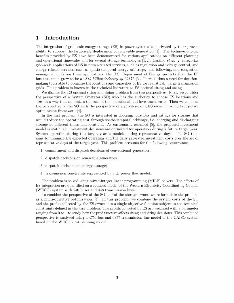
1 Introduction
The integration of grid-scale energy storage (ES) in power systems is motivated by their provenability to support the large-scale deployment of renewable generation [1]. The techno-economicbenefits provided by ES have been demonstrated for various applications on different planningand operational timescales and for several storage technologies [1, 2]. Castillo et al. [2] categorizegrid-scale applications of ES in power-related services, such as regulation and voltage control, andenergy-related services, such as spatio-temporal energy arbitrage, load following, and congestionmanagement. Given these applications, the U.S. Department of Energy projects that the ESbusiness could grow to be a “$19 billion industry by 2017” [3]. There is thus a need for decision-making tools able to optimize the locations and capacities of ES for realistically large transmissiongrids. This problem is known in the technical literature as ES optimal siting and sizing.
We discuss the ES optimal siting and sizing problem from two perspectives. First, we considerthe perspective of a System Operator (SO) who has the authority to choose ES locations andsizes in a way that minimizes the sum of the operational and investment costs. Then we combinethe perspective of the SO with the perspective of a profit-seeking ES owner in a multi-objectiveoptimization framework [4].
In the first problem, the SO is interested in choosing locations and ratings for storage thatwould reduce the operating cost through spatio-temporal arbitrage, i.e. charging and dischargingstorage at different times and locations. As customarily assumed [5], the proposed investmentmodel is static, i.e. investment decisions are optimized for operation during a future target year.System operation during this target year is modeled using representative days. The SO thenaims to minimize the expected operating and the daily pro-rated investment costs over the set ofrepresentative days of the target year. This problem accounts for the following constraints:
1. commitment and dispatch decisions of conventional generators;
2. dispatch decisions on renewable generators;
3. dispatch decisions on energy storage;
4. transmission constraints represented by a dc power flow model.
The problem is solved using mixed-integer linear programming (MILP) solvers. The effects ofES integration are quantified on a reduced model of the Western Electricity Coordinating Council(WECC) system with 240 buses and 448 transmission lines.
To combine the perspective of the SO and of the storage owner, we re-formulate the problemas a multi-objective optimization. [4]. In this problem, we combine the system costs of the SOand the profits collected by the ES owner into a single objective function subject to the technicalconstraints defined in the first problem. The profits collected by ES are weighted with a parameterranging from 0 to 1 to study how the profit motive affects siting and sizing decisions. This combinedperspective is analysed using a 4754-bus and 6377-transmission line model of the CAISO systembased on the WECC 2024 planning model.
3

2 Storage siting and sizing from a centralized perspective
2.1 Problem formulation
From a centralized perspective, the siting and sizing of energy storage should be such that itminimizes the sum of the operating cost and of the investment cost, subject to constraints onthe operation of the system and on the size and location of the investments in energy storage.Appendix B shows how this problem can be formulated mathematically as a Mixed Integer LinearProgramming (MILP) problem. Since one of the reasons for deploying energy storage is to assistin the integration of renewable energy sources such as wind and solar, and since these resourceshave a stochastic output, this optimization relies on a stochastic formulation.
2.2 Case study
This optimization was applied to the simplified model of the WECC system described in [6], whosenetwork consists of 240 buses, 448 transmission lines, 157 aggregated conventional generators (71thermal units, 27 hydropower plants) and a substantial renewable generation portfolio (3 biomass,6 geothermal, 11 generic renewable, 7 solar, and 32 wind farms). Five representative days wereused to represent the variety of load and renewable conditions that should be expected. Thesedays and the weight that each of them should have in the objective function were selected usingthe recursive hierarchical clustering algorithm described in [7].
An energy-to-power ratio of 6 hours was selected for prospective ES investments [8, 9]. EScharging and discharging efficiencies are assumed to be 0.9. Two capital cost scenarios wereconsidered: In the Low Investment Cost (LIC) scenario, the cost of energy storage system isassumed to be $20/kWh and $500/kW, while in the High Investment Cost (HIC) scenario, it isassumed to be $100/kWh and $1500/kW. These investment costs are prorated on a daily basisassuming and ES lifetime is 10 years and an annual discount rate is 5%, as explained in [8]. Weassume that energy storage can be installed at any bus in the system.
To account for future increases in the operating cost of fossil-fuel generators (e.g. due toa carbon tax), the marginal cost of the thermal units was multiplied by a factor of 2, unlessotherwise specified. The production from renewable sources was increased by 40% to simulateCalifornia’s renewable energy goal for the year 2030 [10], unless otherwise stated.
All simulations were carried out on an Intel Xenon 2.55 GHz processor with 32 GB of RAMusing the Hyak supercomputer system at the University of Washington, [11] running CPLEX [12]under GAMS 23.7 [13]. The stopping criterion for all simulations was reaching a 1% optimalitygap.
2.3 Optimal siting decisions
Table 1 summarizes the optimal ES siting decisions as a function of several parameters:
1. the capital cost of deploying energy storage (LIC and HIC scenarios);
2. the value attached to spillage of renewable energy sources V oRS (According to [14], weassume that the value of renewable spillage ranges from $0/MWh to $80/MWh.)
3. the maximum number of locations where energy storage can be installed (1, 5, 10, and 15locations). ES systems located at each bus have a maximum energy rating of S = 25 MWh.
These results show that bus 155 is clearly the preferred location for the deployment of energystorage because storage is located there when only deployment is allowed at only one location andwhen deployment is allowed at 5, 10 or 15 locations, regardless of the value of V oRS and the
4

capital cost scenario. This bus is connected to a transmission line that is prone to congestion.Buses 90, 150, and 239, are selected as potential ES locations for all values of V oRS. All thesebuses are at the end of congested transmission lines.
For the HIC scenario, the optimization determines that installing storage at all 10 or 15 busesis not economically justifiable, except for V oRS = 80$/MWh.
The Venn diagram of Fig. 1 shows the similarity between the siting decisions for NES = 10and different values of V oRS.
TABLE 1. Storage Siting Decisions. Impact of the Investment Cost, V oRS, andNES.
InvestmentVoRS
Maximum number of storage locations
cost 1 5 10 15
LIC
0
155 90 88 142 33 89 142
150 89 150 80 90 160
155 90 155 82 91 228
228 91 228 87 140 239
239 140 239 88 141 240
40
155 27 22 30 88 148 198
28 23 90 89 149 225
90 26 150 90 150 226
150 27 155 140 154 227
155 28 239 142 155 239
80
155 90 31 150 29 148 224
150 33 155 30 149 225
155 49 226 33 150 226
226 90 227 89 155 227
227 148 239 90 198 239
HIC
0
155 88 90 26 88 141
89 155 27 89 142
90 28 90 155
150 29 91 239
155 30 140
40
155 89 80 150 33 90 150
90 83 155 82 91 155
150 88 239 83 140 227
155 89 88 141 239
239 90 89 142
80
155 90 82 155 88 142 224
150 83 198 89 148 225
155 89 226 90 150 226
226 90 227 91 155 227
227 150 239 140 198 239
5

Fig. 1. Venn diagram for the storage siting decisions corresponding to NES = 10 buses: A) Low investment costscenario, and B) high investment cost scenario.
2.4 Optimal sizing decisions
Figures 2 and 3 show the ES sizing decisions corresponding to the siting decisions shown in Table1.
As one would expect, the amount of energy storage installed under the HIC scenario is usuallysmaller than under the LIC scenario.
For the LIC, the optimization deploys at each bus the maximum energy rating allowed at ateach bus (S).
For the highest V oRS, the total installed power capacity increases linearly with the number ofstorage locations NES . For lower V oRS, this total installed power capacity tends to saturate asthe number of locations increases.
6

1-bus 5-bus 10-bus 15-bus0
100
200
300
400
En
erg
y r
atin
g (
MW
h)
1-bus 5-bus 10-bus 15-bus0
100
200
300
400
Po
wer
rat
ing
(M
W)
1-bus 5-bus 10-bus 15-bus0
100
200
300
400
En
erg
y r
atin
g (
MW
h)
1-bus 5-bus 10-bus 15-bus0
100
200
300
400
Po
wer
rat
ing
(M
W)
1-bus 5-bus 10-bus 15-bus0
100
200
300
400
En
erg
y r
atin
g (
MW
h)
1-bus 5-bus 10-bus 15-bus0
100
200
300
400
Po
wer
rat
ing
(M
W)
1st bus
2nd bus
3rd bus
4th bus
5th bus
6th bus
7th bus
8th bus
9th bus
10th bus
11th bus
12th bus
13th bus
14th bus
15th bus
A.1) A.2)
B.2)B.1)
C.1) C.2)
Fig. 2. Energy and power ratings for the low investment cost scenario: A.1)–A.2) V oRS = 0 $/MWh, B.1)–B.2)V oRS = 40 $/MWh, and C.1)–C.2) V oRS = 80 $/MWh.
1-bus 5-bus 10-bus 15-bus0
100
200
300
400
En
erg
y r
atin
g (
MW
h)
1-bus 5-bus 10-bus 15-bus0
100
200
300
400
Po
wer
rat
ing
(M
W)
1-bus 5-bus 10-bus 15-bus0
100
200
300
400
En
erg
y r
atin
g (
MW
h)
1-bus 5-bus 10-bus 15-bus0
100
200
300
400
Po
wer
rat
ing
(M
W)
1-bus 5-bus 10-bus 15-bus0
100
200
300
400
En
erg
y r
atin
g (
MW
h)
1-bus 5-bus 10-bus 15-bus0
100
200
300
400
Po
wer
rat
ing
(M
W)
1st bus
2nd bus
3rd bus
4th bus
5th bus
6th bus
7th bus
8th bus
9th bus
10th bus
11th bus
12th bus
13th bus
14th bus
15th bus
A.1) A.2)
B.1) B.2)
C.1) C.2)
Fig. 3. Energy and power ratings for the high investment cost scenario: A.1)–A.2) V oRS = 0 $/MWh, B.1)–B.2)V oRS = 40 $/MWh, and C.1)–C.2) V oRS = 80 $/MWh.
7

2.5 Cost savings and renewable energy spillage
For a given amount of investment, performing spatio-temporal reduces the system operating cost(i.e. the fuel cost). Fig. 4 shows the savings achieved for both capital cost scenarios, for thevarious number of storage locations and V oRS. These savings are below 1% for this case study.Furthermore, they decrease as V oRS increases as the emphasis shifts to avoiding spilling energyproduced by renewable sources.
0 40 80
VoRS ($/MWh)
0
0.2
0.4
0.6
0.8
1
Fuel
cost
sav
ings
(%)
A) Low investment cost
0 40 80
VoRS ($/MWh)
0
0.2
0.4
0.6
0.8
1
Fuel
cost
sav
ings
(%)
B) High investment cost
1-bus allocation
5-bus allocation
10-bus allocation
15-bus allocation
Fig. 4. Fuel cost savings for: A) Low investment cost scenario, and B) high investment cost scenario.
Fig. 5 shows how renewable energy spillage is reduced for these various conditions. Note thatthis reduction is a by-product of the optimization process and is not explicitly minimized. Thisexplain it increases in some cases.
0 40 80
VoRS ($/MWh)
-1.5
-1
-0.5
0
0.5
1
1.5
2
2.5
3
Ren
ewab
le s
pil
lage
reduct
ion (
%)
A) Low investment cost
0 40 80
VoRS ($/MWh)
-1.5
-1
-0.5
0
0.5
1
1.5
2
2.5
3
Ren
ewab
le s
pil
lage
reduct
ion (
%)
B) High investment cost
1-bus allocation
5-bus allocation
10-bus allocation
15-bus allocation
Fig. 5. Reduction of renewable spillage for: A) Low investment cost scenario, and B) high investment cost scenario.
2.6 Profitability of energy storage
While this model focuses on determining the location and size of storage that would minimize thetotal cost, it is useful to consider how profitable storage would be under these conditions. Fig.6 shows the operating profit collected by the energy storage systems if they bought and sold theenergy they charge and discharge at the marginal price for the bus where they are located. Theoperational profit increases with the number of ES locations and V oRS.
However, the operating profit is only one side of profitability. Taking into account the invest-ment cost, Fig. 7 shows the rate of return ratio of energy storage, i.e. its ability to recover theinvestment cost. These results show that ES is profitable only for a small number of ES locations
8

in the LIC scenario. In general, this rate of return ratio increases with V oRS. Policy decisions thatdiscourage spillage of energy produced from renewable energy sources could therefore significantlyimprove the profitability of investments in energy storage. This rate of return ratio decreases withthe number of ES locations regardless of V oRS or the capital cost scenario. This suggests thata coordinated strategy for investments in energy storage may be needed to ensure the economicviability of these investments.
0 40 80
VoRS ($/MWh)
0
0.5
1
1.5
2
2.5
3
To
tal
op
erat
ion
al p
rofi
ts (
10
4 $
)
A) Low investment cost
0 40 80
VoRS ($/MWh)
0
0.5
1
1.5
2
2.5
3
To
tal
op
erat
ion
al p
rofi
ts (
10
4 $
)
B) High investment cost
1-bus allocation
5-bus allocation
10-bus allocation
15-bus allocation
Fig. 6. Operating profit of energy storage for: A) Low investment cost scenario, and B) high investment costscenario.
0 40 80
VoRS ($/MWh)
0
0.5
1
1.5
2
2.5
Pro
fit
/ In
ves
tmen
t co
st
A) Low investment cost
0 40 80
VoRS ($/MWh)
0
0.5
1
1.5
2
2.5
Pro
fit
/ In
ves
tmen
t co
st
B) High investment cost
1-bus allocation5-bus allocation10-bus allocation15-bus allocation
Profitable
Nonprofitable
Fig. 7. Rate of return ratio of energy storage for: A) Low investment cost scenario, and B) high investment costscenario.
2.7 Effect of the maximum rating of energy storage systems
Since energy storage systems are quite large, it is reasonable to assume that the amount of storagethat can be installed at each bus is limited. In the previous sections, this amount was limited toS = 25 MWh per bus. In this section, we gradually increase S up to 100 MWh per bus for theLIC scenario, with V oRS = 0 $/MWh, and NES = 10.
Figures 8 and 9 show how the optimal siting and sizing decisions change as we increase S.These results show that the siting decisions are robust with respect to the maximum energy ratingof energy storage at each bus. Specifically, buses 90, 150, 155, and 239 remain the best locationsfor all cases. In terms of the sizing decisions, Fig. 9 shows that the energy ratings are limited byS and that the power ratings increase with this parameter.
9

Fig. 8. Venn diagram showing how optimal storage siting decisions change as a function of the maximum energystorage rating per bus S. The numbers in bold are the common storage locations regardless the V oRS for the low
investment cost.
25 50 75 100
Maximum energy storage rating (MWh)
0
200
400
600
800
1000
En
erg
y r
atin
g (
MW
h)
25 50 75 100
Maximum energy storage rating (MWh)
0
200
400
600
800
1000
Po
wer
rat
ing
(M
W)
1st bus 2nd bus 3rd bus 4th bus 5th bus 6th bus 7th bus 8th bus 9th bus 10th bus
Fig. 9. Effect of the maximum energy storage rating per bus S on the energy and power ratings.
Figure 10 shows the effect of S. The cost savings (A) and the operating profits (B) increase withS, while the amount of renewable energy spilled displays a non-monotonic behavior (C).Althoughthe operating profit increases, the rate of return ratio decreases due to the higher investment cost(D).
2.8 Effect of the cost of thermal generation
An increase in the cost of thermal generation, coupled with an increase in the amount of energyproduced from renewable energy sources, is likely to increase arbitrage opportunities. We analyzethis effect by progressively increasing the marginal cost of conventional thermal generators. Weconsider the LIC scenario, with V oRS = 0 $/MWh, NES = 10, and S = 100 MWh because thisis the case providing the largest cost savings. In this case, there is a 49.6% of installed renewablegeneration capacity including hydropower with respect to the overall installed capacity.
Figure 11 is a Venn diagram which shows that the siting decisions remain quite robust as themarginal cost is multiplied by a factor ranging from 1 to 5. In particular, buses 90, 150, 155, and239 are selected as optimal locations irrespective of the value of this marginal cost.
10

25 50 75 100
Maximum energy storage rating (MWh)
0
0.2
0.4
0.6
0.8
1
1.2
Fu
el c
ost
sav
ing
s (%
)
25 50 75 100
Maximum energy storage rating (MWh)
0
0.5
1
1.5
2
2.5
3
Tota
l oper
atio
nal
pro
fits
(10
4 $
)
25 50 75 100
Maximum energy storage rating (MWh)
-2
-1
0
1
2
3
4
Ren
ewab
le s
pil
lag
e re
du
ctio
n (
%)
25 50 75 100
Maximum energy storage rating (MWh)
0
0.2
0.4
0.6
0.8
1
Pro
fit
/ In
ves
tmen
t co
st
A) B)
D)C)
Nonprofitable
Fig. 10. Effect of the maximum energy rating S on A) fuel cost savings, B) operating profits, C) reduction inrenewable energy spillage, and D) ES rate of return ratio.
Fig. 11. Venn diagram showing the effect of the marginal costs of conventional generators on the optimal storagesiting decisions. The numbers in bold are the common storage locations regardless the V oRS and the maximum
energy storage rating per bus S for the low investment cost.
Fig. 12 shows that the optimal total power rating of BESS tends to saturate as the marginalcosts of thermal generation increases.
Figure 13 shows how this marginal cost increase would affect the cost savings, the operationalprofit, the amount of renewable energy spillage reduction and the rate of return of energy storage.
11

1 2 3 4 5
Relative increase in marginal costs
0
200
400
600
800
1000
Ener
gy r
atin
g (
MW
h)
1 2 3 4 5
Relative increase in marginal costs
0
200
400
600
800
1000
Pow
er r
atin
g (
MW
)
1st bus
2nd bus
3rd bus
4th bus
5th bus
6th bus
7th bus
8th bus
9th bus
10th bus
Fig. 12. Effect of the marginal costs of thermal generators on the energy and power ratings of energy storage.
1 2 3 4 5
Relative increase in marginal costs
0
0.2
0.4
0.6
0.8
1
1.2
Fu
el c
ost
sav
ings
(%)
1 2 3 4 5
Relative increase in marginal costs
0
2
4
6
8
To
tal
oper
atio
nal
pro
fits
(1
04 $
)
1 2 3 4 5
Relative increase in marginal costs
0
0.2
0.4
0.6
0.8
1
Ren
ewab
le s
pil
lage
red
uct
ion (
%)
1 2 3 4 5
Relative increase in marginal costs
0
0.2
0.4
0.6
0.8
1
Pro
fit
/ In
ves
tmen
t co
st
A)
C)
B)
D) Profitable
No Profitable
Fig. 13. Effect of the marginal costs of conventional thermal generators on A) Fuel cost savings, B) operationalprofits, C) reduction of renewable spillage, and D) ES rate of return ratio.
2.9 Effect of the proportion of production from renewable sources
To study the effect of stringent renewable energy goals similar to those imposed by the state ofCalifornia by 2030 or Hawaii for the years 2030 and 2040 [10], the original renewable productionis multiplied by a factor ranging from 1 to 1.8. We assume that the locations of this renewableproduction remain unchanged. The other fixed parameters are the same as in the previous section.
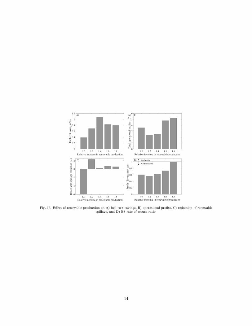
The Venn diagram of Fig. 20 shows that once again the ES siting decisions remain robustagainst changes in the penetration of renewable production. Buses 90, 150, 155, and 239 are stillselected regardless of the renewable scenario. On the other hand, the optimal power ratings (Fig.15) do not increase with the renewable penetration. This effect has an impact on the fuel costsavings and operational profits given in Fig. 16, which shows that the maximum cost savings are notattained for the maximum renewable penetration. However, an increased renewable penetrationimproves the operating profits and the rate of return ratio of energy storage and reduces the
12

amount of renewable energy spilled.
Fig. 14. Venn diagram showing the effect of renewable production on optimal storage siting decisions. Thenumbers in bold are the common storage locations regardless the V oRS, the maximum energy storage rating per
bus S, and the marginal costs of thermal generators for the low investment cost.
1.0 1.2 1.4 1.6 1.8
Relative increase in renewable production
0
200
400
600
800
1000
Ener
gy r
atin
g (
MW
h)
1.0 1.2 1.4 1.6 1.8
Relative increase in renewable production
0
200
400
600
800
1000
Pow
er r
atin
g (
MW
)
1st bus
2nd bus
3rd bus
4th bus
5th bus
6th bus
7th bus
8th bus
9th bus
10th bus
Fig. 15. Effect of renewable production on the optimal energy and power ratings.
13
1.0 1.2 1.4 1.6 1.8
Relative increase in renewable production
0
0.2
0.4
0.6
0.8
1
1.2
Fu
el c
ost
sav
ing
s (%
)
1.0 1.2 1.4 1.6 1.8
Relative increase in renewable production
0
1
2
3
4
5
6
To
tal
op
erat
ion
al p
rofi
ts (
10
4 $
)
1.0 1.2 1.4 1.6 1.8
Relative increase in renewable production
-6
-4
-2
0
2
Ren
ewab
le s
pil
lag
e re
du
ctio
n (
%)
1.0 1.2 1.4 1.6 1.8
Relative increase in renewable production
0
0.2
0.4
0.6
0.8
1
Pro
fit
/ In
ves
tmen
t co
st
A) B)
C) D) Profitable
No Profitable
Fig. 16. Effect of renewable production on A) fuel cost savings, B) operational profits, C) reduction of renewablespillage, and D) ES rate of return ratio.
14
2.10 Simultaneous effect of the cost of thermal generation and propor-tion of production from renewable sources
Assuming the case providing the largest cost savings, i.e. LIC scenario, with V oRS = 0 $/MWh,NES = 10, and S = 100 MWh, we analyze the effect of simultaneous increases in the cost of thermalgeneration and in the amount of energy produced from renewable energy sources. This scenario isa realistic anticipation of what might happen in coming years: as the amount of renewable energyproduction increases, the cost of conventional generation is likely to increase to compensate forthe fact that these generators will produce less but will still have to cover their fixed costs. Fivecases are simulated by increasing the original cost of thermal generation and the original renewableproduction by the following factors: 1 and 1 (case a), 2 and 1.2 (case b), 3 and 1.4 (case c), 4 and1.6 (case d), and 5 and 1.8 (case e).
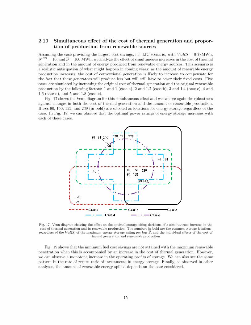
Fig. 17 shows the Venn diagram for this simultaneous effect and we can see again the robustnessagainst changes in both the cost of thermal generation and the amount of renewable production.Buses 90, 150, 155, and 239 (in bold) are selected as locations for energy storage regardless of thecase. In Fig. 18, we can observe that the optimal power ratings of energy storage increases witheach of these cases.
Fig. 17. Venn diagram showing the effect on the optimal storage siting decisions of a simultaneous increase in thecost of thermal generation and in renewable production. The numbers in bold are the common storage locations
regardless of the V oRS, of the maximum energy storage rating per bus S, and the individual effects of the cost ofthermal generation and renewable production.
Fig. 19 shows that the minimum fuel cost savings are not attained with the maximum renewablepenetration when this is accompanied by an increase in the cost of thermal generation. However,we can observe a monotone increase in the operating profits of storage. We can also see the samepattern in the rate of return ratio of investments in energy storage. Finally, as observed in otheranalyses, the amount of renewable energy spilled depends on the case considered.
15

a b c d e0
200
400
600
800
1000
Ener
gy r
atin
g (
MW
h)
Casea b c d e
0
200
400
600
800
1000
Pow
er r
atin
g (
MW
)
Case
1st bus
2nd bus
3rd bus
4th bus
5th bus
6th bus
7th bus
8th bus
9th bus
10th bus
Fig. 18. Effect of renewable production on the optimal energy and power ratings.
a b c d e0
0.2
0.4
0.6
0.8
1
Fuel
cost
sav
ings
(%)
Casea b c d e
0
5
10
15
Tota
l o
per
atio
nal
pro
fits
(104
$)
Case
a b c d e−1
0
1
2
3
Ren
ewab
le s
pil
lag
e re
du
ctio
n (
%)
Casea b c d e
0
0.5
1
1.5
Pro
fit
/ In
ves
tmen
t co
st
Case
No Profitable
Profitable
D)
A) B)
C)
Fig. 19. Effect of renewable production on A) fuel cost savings, B) operating profit of energy storage, C) reductionin renewable energy spillage, and D) ES rate of return ratio.
16

3 Combining cost minimization and profitability of storage
3.1 Problem formulation
In a competitive electricity market environment, investments in energy storage systems will bemade by for-profit entities. While the availability of these storage devices should lower the costof operating the system, this is not the same as maximizing the operating profit collected byenergy storage systems. The objectives of the system operator and of the storage owners arethus not aligned. We formulate a multi-objective optimization problem, which combines the costminimization with the profit maximization. By adjusting the weight given to each part of theobjective function, we can study the interactions between the goals of the system operator and thestorage owner.
Appendix C provides a detailed mathematical formulation of this multi-objective optimizationproblem and a description of a two-stage algorithm that makes possible its application to large-scalesystems.
3.2 Case study
This multi-objective optimization approach was applied to a model of the CAISO system based onthe WECC 2024 planning model. Table 2 summarizes the characteristics of this system. As in theprevious problem, investments decisions are based on 5 representative days and their associatedweights determined using the recursive hierarchical clustering algorithm described in [7]. Anenergy-to-power ratio of 6 hours was selected for prospective ES investments [8,9]. Energy storagecharging and discharging efficiencies are assumed to be 0.9.
TABLE 2. Characteristics of the CAISO System Model.
Controllable generators 316
Buses 4,754
Transmission Lines 6,377
Wind generators 117
Solar generators 414
Uncontrollable resources or fixed generation 1,182
In order to reduce the computational burden and to focus on the multi-objective problem,we perform siting and sizing decisions for the Sacramento Municipal District area which has 245buses. We assume that spilling renewable energy has a value of 50 $/MWh, and that the maximumnumber of locations where storage can be installed is 10. We consider only the lower investmentcost scenario (500 $/kWh and 20 $/kW) and we limit the maximum energy storage rating at eachbus to 50 MWh. The locational marginal prices are assumed to be equal to those resulting fromthe system cost minimization problem without ES. Generation considered as ”fixed” in the WECCmodel occasionally needs to be reduced to ensure feasibility. Appendix D discusses the policiesused to determine fixed generation spillage.
3.3 Base case
We establish a base case by solving the cost minimization problem for the system without en-ergy storage. We first perform this optimization for each representative day separately and onestochastic optimization. We then perform a stochastic optimization where each representative dayis weighted by the number of days in the cluster it represents. These results give us a basis to
17

assess the benefits of integrating energy storage in the system. Table 3 shows the total generationcost, the total renewable spillage including solar and wind assets, and the total fixed generationspillage for each representative day and for the stochastic optimization.
TABLE 3. Costs for the base case without energy storage
Generation cost ($) Renewable spillage (MW) Fixed spillage (MW)
Day 1 4328530.9 25521.8 28435.1
Day 2 10764202.5 15.1 59081.0
Day 3 13336594.2 7855.6 64688.0
Day 4 3823475.6 39079.2 28120.7
Day 5 11005584.4 1218.8 55147.3
Stochastic 9030299.8 12096.4 47727.7
3.4 Balancing cost and profit
The formulation of the multi-objective optimization problem involves a parameter β which weighsthe importance given to the profit collected by the energy storage systems. If the value of thisparameter is zero, this profit is not taken into account in the optimization. We perform simulationsfor 4 values of the parameter β (0.001, 0.01, 0.1 and 1), thus giving an increasing weight to themaximization of the profit over the minimization of the cost. Table 4 gives the ten best locationsfor siting storage for each value of β. Four locations (buses 4337, 4375, 4376, 4523) are selectedfor all these values of β. On the other hand, two buses (2374 and 4361) are selected only for β =0.001 which almost neglects the profit part of the objective function. These are buses that wouldbe of interest to the system operator but not to independent investors.
Figure 20 shows the optimal energy and power ratings for all energy storage locations given inTable 4. The energy rating is limited by the artificially imposed 50 MWh bound. The power ratingincreases slightly as the profit maximization gains more importance in the objective function.
0.001 0.01 0.1 1
β
0
100
200
300
400
500
En
erg
y r
atin
g,
MW
h
0.001 0.01 0.1 1
β
0
100
200
300
400
500
Po
wer
rat
ing
, M
W
1st bus
2nd bus
3rd bus
4th bus
5th bus
6th bus
7th bus
8th bus
9th bus
10th bus
Fig. 20. Optimal energy and power ratings for weights of the profit motive
Figure 21 shows how the multi-objective optimization balances the profit against the operatingcost savings for these values of the factor β. As expected, the cost savings decrease as we increasethe importance of the profit collected by the energy storage owner. Going from β = 0.001 and
18

TABLE 4. Effect of the profit motive on the optimal siting decisions
β
0.001 0.01 0.1 1
1st 2374 4265 4259 4210
2nd 4259 4266 4265 4259
3rd 4337 4336 4337 4265
4th 4360 4337 4360 4267
5th 4361 4375 4375 4336
6th 4375 4376 4376 4337
7th 4376 4523 4382 4338
8th 4523 4528 4403 4375
9th 4528 4537 4523 4376
10th 4543 4543 4543 4523
β = 0.01 increases the profit of the storage owner by 64% at the expense of a 16% reduction inthe cost savings that storage creates in the system. Increasing β from 0.1 to 1.0 leads to negativecost savings (i.e. a net increase in system cost!) but raises the profits by only 4%. Investmentscorresponding to the range from β = 0.01 to β = 0.1 are thus most likely to be both profitable forinvestors and valuable from an overall system perspective.
Figure 22 show how balancing cost and profit affects the total spillage of renewable energy andthe total congestion surplus. The smallest amount renewable spillage is achieved for the lowestvalue of β. A moderate weight given to the profit motive minimizes the congestion surplus.
3.5 Effect of the number of storage locations
Figure 23 shows how the curve relating the total cost savings and the profit changes when we allowstorage to be installed at 1, 5 or 10 locations. As expected, both the profit and the cost savingsincrease as we allow more storage installations. These curves suggest that allowing storage at morelocations makes it possible to reduce costs while increasing profits. With fewer locations, thesetwo objectives are more antagonistic.
19

-0.1 0 0.1 0.2 0.3 0.4 0.5
Cost savings (%)
2.5
3
3.5
4
4.5
5
5.5
6
6.5
To
tal
pro
fit
(M$
)
β = 1β = 0.1
β = 0.01
β = 0.001
Fig. 21. Cost savings versus total profits
0.001 0.01 0.1 1
β
1.15
1.16
1.17
1.18
1.19
1.2
1.21
1.22
Tota
l re
new
able
spil
lage
(MW
)
×104
0.001 0.01 0.1 1
β
2.5
3
3.5
Tota
l co
nges
tion s
urp
lus
(M$)A) B)
Fig. 22. Effect of balancing cost and profit on A) total renewable spillage and B) congestion surplus
20

-0.1 0 0.1 0.2 0.3 0.4 0.5
Cost savings, %
0
1
2
3
4
5
6
7
To
tal
pro
fit,
M$
1-bus allocation
5-bus allocation
10-bus allocation
β = 1
β = 1
β = 1
β = 0.1
β = 0.1
β = 0.1
β = 0.01
β = 0.01
β = 0.01
β = 0.001
β = 0.001
β = 0.001
Fig. 23. Effect of the number of storage locations on the total cost savings and profit
21

4 Conclusions
This report considers the optimal siting and sizing of energy storage in large power systems from twodifferent perspectives. First, those decisions are optimized from a centralized, cost minimizationperspective.Then, a multi-objective optimization is used to examine how this cost minimizationis related to the profit maximization that would be the goal of independent investors in energystorage. Both approaches are tested on realistic models of large power systems. The followingobservations can be made based on the result of the centralized, cost minimization formulation:
1. Reducing the penalty for spilling energy from renewable energy sources reduces the systemoperating cost but reduces the profit collected by the storage owners.
2. Storage tends to reduce renewable energy spillage, but this is not always the case.
3. Operating storage to minimize the total operating cost does not guarantee that investmentsin storage will be profitable. Including minimum profit constraints is therefore needed inmodels used for selecting investments in storage systems.
4. The proposed method is able to identify favorable storage locations on large systems.
5. These siting decisions are generally robust against the size of penalties for spilling renewableenergy, the maximum allowed size of storage systems, and future projections of conventionalunits’ marginal costs and increasing renewable production.
Considering both the cost savings resulting from the deployment of energy storage and theprofitability of this storage leads to the following observations:
1. The siting decisions depend on the relative weight given to cost minimization and profitmaximization.
2. The energy rating is limited by the artificial 50-MWh limit imposed on the size of energystorage systems. On the other hand the power rating increase when more weight is given toprofit maximization.
3. Lower values of the weighting parameter β lead to a better trade-off between cost and profit.
4. Changing the relative weight of the cost and profit in the optimization does not significantlychange the amount of renewable energy spilled or the congestion surplus.
5. Both the cost savings and the profits increase with the number of energy storage locations.
22

A Nomenclature
Sets and indices
B Set of buses, indexed by b.
B Set of buses where ES can be installed, indexed by b.
E Set of representative days, indexed by e.
Ωg(Ωgb) Set of conventional or controllable generators (connected to bus b), indexed by i.
Ωrg(Ωrgb ) Set of renewable generators (connected to bus b), indexed by r.
Ωhp(Ωhpb ) Set of hydro generators (connected to bus b), indexed by h.
L Set of transmission lines, indexed by l.
Oi Set of segments of the cost curve of conventional generator i, indexed by o.
T Set of time intervals, indexed by t.
n Auxiliary index of time intervals.
o(l), d(l) Indices of origin and destination buses of line l.
Variables
All variables are per period t and representative day e unless otherwise indicated.
chtbe Charging rate of the energy storage system connected to bus b.
cmaxb Maximum power rating of the energy storage system connected to bus b.
distbe Discharging rate of the energy storage system connected to bus b.
pftle Power flow on line l.
pgtie Power output of conventional generator i.
pgtioe Power output on segment o of the cost curve of generator i.
phpthe Power output of hydro generator h.
stbe State-of-charge of the energy storage system connected to bus b.
smaxb Maximum energy rating of the storage system connected to bus b.
sprgtre Power spillage of renewable generator r.
vtie On/off status of conventional generator i.
ytie Start-up status of conventional generator i.
ztie Shutdown status of conventional generator i.
αtbe Binary variable representing whether an energy storage system is charging (1) or dis-charging (0).
βtbe Auxiliary continuous variable representing the nonlinear product chtbeαtbe.
θtbe Voltage phase angle at bus b.
σb Binary variable corresponding to the decision to locate an energy storage system atbus b.
23

Parameters
C Maximum power rating of an energy storage system.
CEioe Marginal cost of segment o of the cost curve of conventional generator i on represen-
tative day e.
CSUi Start-up cost of conventional generator i.
CS Capital cost of an energy storage system per MWh.
CP Capital cost of an energy storage system per MW.
DTi Minimum down time of conventional generator i.
Dtbe Demand at bus b during period t on representative day e.
NES Number of energy storage locations.
NDTie Number of periods during which unit i must be initially scheduled off due to its mini-
mum down time constraint on representative day e.
NUTie Number of periods during which unit i must be initially scheduled on due to its mini-
mum up time constraint on representative day e.
Pf
l Maximum power flow on line l.
Pg
ioe Maximum power output on segment o of the cost curve of conventional generator i onrepresentative day e.
Pg
ie Maximum power output of conventional generator i on representative day e.
P gie Minimum power output of conventional generator i on representative day e.
Phpthe Minimum power output of hydro plant h during time period t on representative day e.
Php
the Maximum power output of hydro plant h during time period t on representative daye.
P rgtre Power output of renewable generator r during time period t on representative day e.
RDi Maximum ramp down rate of conventional generator i.
RUi Maximum ramp up rate of conventional generator i.
S Maximum energy rating of an energy storage system.
UTi Minimum up time of conventional generator i.
V 0ie Initial commitment of conventional generator i on representative day e.
V oRS Value of renewable spillage.
xl Reactance of line l.
ρ Energy-to-power ratio of an energy storage system.
ηc/d Charging/discharging efficiency of energy storage system.
µe Relative frequency of representative day e.
24

B Mathematical formulation of the cost minimization prob-lem
The notation used in this formulation can be found in Appendix A. The objective function is:
Minimize∑e∈E
[µe
∑t∈T
∑i∈Ωg
(∑o∈Oi
CEioep
gtioe + CSU
i ytie
)]+
∑e∈E
[µe
∑t∈T
∑r∈Ωrg
V oRSsprgtre
]+∑b∈B
(CSsmax
b + CP cmaxb
), (1)
where the first term represents the expected operating cost over the representative days, includingthe dispatch and commitment costs of conventional generation; the second term is the expectedvalue of the renewable energy spilled; and the last term denotes the daily pro-rated investmentcost in energy storage, where parameters CS and CP are calculated based on the net present valueapproach [8].
The following subsections describe the constraints on this optimization problem.
Binary variables logic
The binary on/off status, start-up, and shutdown decisions are formulated as follows:
ytie − ztie = vtie − vt−1,ie;∀t ∈ T ,∀i ∈ Ωg,∀e ∈ E (2)
ytie + ztie ≤ 1;∀t ∈ T ,∀i ∈ Ωg,∀e ∈ E . (3)
Constraint (2) determines whether unit i is started up or shut down at time t of representativeday e based on the change in its on/off status between operating intervals t and t− 1. Constraint(3) ensures that unit i cannot be started up and shut down during the same time interval of therepresentative day e.
Inter-temporal constraints
These constraints are modeled as:
vtie = V 0ie;∀t ≤ NUT
ie +NDTie ,∀i ∈ Ωg,∀e ∈ E (4)
t∑n=t−UTi+1
yrie ≤ vtie;∀t ∈[NUT
ie , nT],∀i ∈ Ωg,∀e ∈ E (5)
t∑n=t−DTi+1
zrie ≤ 1− vtie;∀t ∈[NDT
ie , nT],∀i ∈ Ωg,∀e ∈ E (6)
−RDi ≤ pgtie − pgt−1,ie ≤ RUi;∀t ∈ T ,∀i ∈ Ωg,∀e ∈ E . (7)
Constraints (4)–(6) enforce the minimum up and down times. Constraint (7) models the ramprate limits of the conventional units.
25

Generation dispatch constraints
The power outputs of conventional units, hydropower plants, and renewable generation units areconstrained as follows:
pgtie =∑o∈Oi
pgtioe;∀i ∈ Ωg,∀t ∈ T ,∀e ∈ E (8)
0 ≤ pgtioe ≤ Pg
ioe;∀o ∈ Oi,∀i ∈ Ωg,∀t ∈ T ,∀e ∈ E (9)
P gie · vtie ≤ p
gtie ≤ P
g
ie · vtie;∀i ∈ Ωg,∀t ∈ T ,∀e ∈ E (10)
Phpthe ≤ p
hpthe ≤ P
hp
the;∀h ∈ Ωhp,∀t ∈ T ,∀e ∈ E (11)
0 ≤ sprgtre ≤ Prgtre;∀r ∈ Ωrg,∀t ∈ T ,∀e ∈ E (12)
Constraints (8)–(9) characterize the block structure of conventional generators. Constraints(10) enforce the minimum and maximum bounds on these units. Constraints (11) keep the hy-dropower production between its minimum and maximum limits. Finally, constraints (12) set thebounds for renewable generation spillage.
Network constraints
Network constraints are implemented using the following dc power flow model:
pftle =1
xl
(θt,o(l),e − θt,d(l),e
),∀t ∈ T ,∀l ∈ L,∀e ∈ E (13)
− P f
l ≤ pftle ≤ P
f
l ,∀t ∈ T ,∀l ∈ L,∀e ∈ E . (14)
Constraint (13) computes the power flows on the network branches. Constraints (14) enforcethe power flow limits.
Power balance constraint
The nodal power balance is formulated as follows:
∑i∈Ωg
b
pgtie +∑
h∈Ωhpb
phpthe +∑
r∈Ωrgb
(P rgtre − sp
rgtre
)−
∑l|o(l)=b
pftle +∑
l|d(l)=b
pftle + distbe = Dtbe + chtbe,
∀t ∈ T ,∀b ∈ B,∀e ∈ E . (15)
Constraint (15) includes the injections of conventional and renewable generation, loads, adjacenttransmission lines, as well as energy storage charging and discharging.
26

Constraints on energy storage systems
The constraints on energy storage systems are formulated as follows:
stbe = st−1,be + chtbeηc − distbe/ηd;∀t ∈ T ,∀b ∈ B,∀e ∈ E (16)
0 ≤ stbe ≤ smaxb ;∀t ∈ T ,∀b ∈ B,∀e ∈ E (17)
0 ≤ chtbeηc ≤ cmaxb αtbe;∀t ∈ T ,∀b ∈ B,∀e ∈ E (18)
0 ≤ distbe/ηd ≤ cmaxb
(1− αtbe
);∀t ∈ T ,∀b ∈ B,∀e ∈ E (19)
cmaxb ρ ≤ smax
b ;∀b ∈ B (20)
0 ≤ smaxb ≤ Sσb;∀b ∈ B (21)
0 ≤ cmaxb ≤ Cσb;∀b ∈ B (22)∑
b∈B
σb ≤ NES . (23)
Constraint (16) computes the ES state-of-charge. Constraints (17), (18)–(19) enforce respec-tively the energy and power ratings of ES. Constraints (18)–(19) preclude ES from simultaneouslycharging and discharging. Constraint (20) relates the energy and power ratings via an energy-powerratio determined by the chosen storage technology. Constraints (21)–(22) limit the maximum ESpower and energy rating at each bus. Finally, constraint (23) allows placing only a number NES
of energy storage system at a subset of buses B.The optimization problem (1)–(23) is a nonlinear program because of the presence of products of
continuous and binary decision variables (cmaxb αtbe) in (18)–(19). These products can be linearized
using integer algebra results [15]. Constraints (18)–(19) can be replaced with:
0 ≤ chtbeηc ≤ βtbe,∀t ∈ T ,∀b ∈ B,∀e ∈ E (24)
0 ≤ distbe/ηd ≤ cmaxb − βtbe,∀t ∈ T ,∀b ∈ B,∀e ∈ E (25)
0 ≤ βtbe ≤ Cαtbe,∀t ∈ T ,∀b ∈ B,∀e ∈ E (26)
0 ≤ cmaxb − βtbe ≤ C
(1− αtbe
),∀t ∈ T ,∀b ∈ B,∀e ∈ E . (27)
The stochastic ES siting and sizing problem to be solved for cost minimization is then theMILP problem given by (1)–(17), (20)–(27).
27
C Mathematical formulation of the multi-objective problem
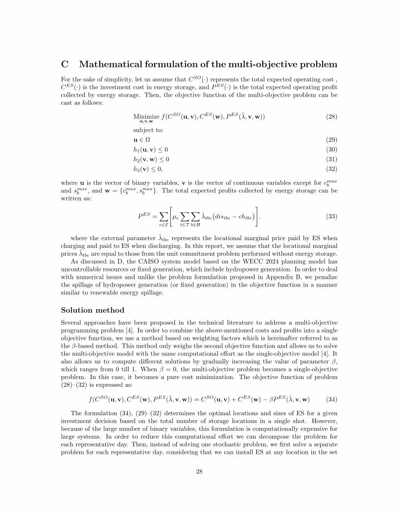
For the sake of simplicity, let us assume that CSO(·) represents the total expected operating cost ,CES(·) is the investment cost in energy storage, and PES(·) is the total expected operating profitcollected by energy storage. Then, the objective function of the multi-objective problem can becast as follows:
Minimizeu,v,w
f(CSO(u,v), CES(w), PES(λ,v,w)) (28)
subject to:
u ∈ Ω (29)
h1(u,v) ≤ 0 (30)
h2(v,w) ≤ 0 (31)
h3(v) ≤ 0, (32)
where u is the vector of binary variables, v is the vector of continuous variables except for cmaxb
and smaxb , and w = cmax
b , smaxb . The total expected profits collected by energy storage can be
written as:
PES =∑e∈E
[µe
∑t∈T
∑b∈B
λtbe(distbe − chtbe
)]. (33)
where the external parameter λtbe represents the locational marginal price paid by ES whencharging and paid to ES when discharging. In this report, we assume that the locational marginalprices λtbe are equal to those from the unit commitment problem performed without energy storage.
As discussed in D, the CAISO system model based on the WECC 2024 planning model hasuncontrollable resources or fixed generation, which include hydropower generation. In order to dealwith numerical issues and unlike the problem formulation proposed in Appendix B, we penalizethe spillage of hydropower generation (or fixed generation) in the objective function in a mannersimilar to renewable energy spillage.
Solution method
Several approaches have been proposed in the technical literature to address a multi-objectiveprogramming problem [4]. In order to combine the above-mentioned costs and profits into a singleobjective function, we use a method based on weighting factors which is hereinafter referred to asthe β-based method. This method only weighs the second objective function and allows us to solvethe multi-objective model with the same computational effort as the single-objective model [4]. Italso allows us to compute different solutions by gradually increasing the value of parameter β,which ranges from 0 till 1. When β = 0, the multi-objective problem becomes a single-objectiveproblem. In this case, it becomes a pure cost minimization. The objective function of problem(28)–(32) is expressed as:
f(CSO(u,v), CES(w), PES(λ,v,w)) = CSO(u,v) + CES(w)− βPES(λ,v,w) (34)
The formulation (34), (29)–(32) determines the optimal locations and sizes of ES for a giveninvestment decision based on the total number of storage locations in a single shot. However,because of the large number of binary variables, this formulation is computationally expensive forlarge systems. In order to reduce this computational effort we can decompose the problem foreach representative day. Then, instead of solving one stochastic problem, we first solve a separateproblem for each representative day, considering that we can install ES at any location in the set
28

Fig. 24. Siting and sizing algorithm for large-scale systems.
of buses B). Then we solve the stochastic problem with a reduced set of buses where ES can beinstalled (Bbest). Therefore, the siting and sizing algorithm is divided into two stages as shown inFig. 24 and the computational effort for solving the stochastic problem is reduced.
29

D Handling of fixed generation
Our model of the CAISO system is based on the WECC 2024 planning model, which includes”uncontrollable resources” or ”fixed generation”. These include hydropower plants. Under somecircumstances, this fixed generation must be adjusted to make the optimization problem feasible.To minimize these deviations, we penalize reductions in the output of these fixed generation sourcesin the objective function in the same way as renewable generation. The penalty for spillage canbe either: (i) the same as the penalty for spilling renewable generation or (ii) Ten times greaterthan the highest V oRS that we consider (i.e. 1000 $/MWh).
The following figures illustrate the effect of these penalties for the case without energy storageand for three different values of the V oRS (0, 50, and 100 $/MWh). Figures 25 and 26 show theeffect of these penalties on the generation costs, the fixed spillage costs, and the renewable costsfor different values of V oRS. They show that the treatment of the fixed generation influencesthe generation and renewable spillage costs. How best to handle these fixed generators in theoptimization would need to be discussed with the system operator.
Fig. 25. Effect of the value of renewable energy spillage on the generation cost, the fixed generation spillage cost,and the renewable spillage cost when the penalty for fixed generation spillage is the same as the value of renewable
energy spillage.
Fig. 26. Effect of the value of renewable energy spillage on the generation cost, the fixed generation spillage cost,and the renewable spillage cost when the penalty for fixed generation spillage is set at 1000 $/MWh
30

References
[1] J. Eyer and Garth Corey, “Energy storage for the electricity grid: Benefits andmarket potential assessment guide,” Technical report, Feb. 2010. [Online]. Avail-able at: http://www.storagealliance.org/sites/default/files/whystorage/Sandia_
Energy_Storage_Guide.pdf
[2] A. Castillo and D. F. Gayme, “Grid-scale energy storage applications in renewable energyintegration: A survey,” Energy Conversion and Management, vol. 87, pp. 885–894, Nov. 2014.
[3] U.S. Department of Energy, “Grid energy storage,” Technical report, Dec. 2013. [Online].Available at: http://www.sandia.gov/ess/docs/other/Grid_Energy_Storage_Dec_2013.pdf
[4] M. Ehrgott, “A discussion of scalarization techniques for multiple objective integer program-ming,” Ann. Oper. Res., no. 147, pp. 343–360, Aug, 2006.
[5] L. Baringo and A. J. Conejo, “Strategic wind power investment,” IEEE Trans. Power Syst.,vol. 29, no. 3, pp. 1250–1260, May 2014.
[6] J. E. Price and J. Goodin, “Reduced network modeling of WECC as a Market Design Pro-totype,” in Proc. of the 2011 IEEE Power and Energy Society General Meeting, 2011, pp.1–5.
[7] B. Pitt, “Applications of data mining techniques to electric load profiling”, PhD thesis, Uni-versity of Manchester, UK, 2000. [Online]. Available at: http://www.ee.washington.edu/
research/real/Library/Thesis/Barnaby_PITT.pdf
[8] H. Pandzic, Y. Wang, T. Qiu, Y. Dvorkin, and D. S. Kirschen, “Near-optimal method forsiting and sizing of distributed storage in a transmission network,” IEEE Trans. Power Syst.,vol. 30, no. 5, pp. 2288–2300, Sep. 2015.
[9] B. Dunn, H. Kamath, and J.-M. Tarascon, “Electrical energy storage for the grid: A batteryof choices,” Science, vol. 334, pp. 928–935, 2011.
[10] “State renewable portfolio standards and goals,” 2016. [Online]. Available at:http://www.ncsl.org/research/energy/renewable-portfolio-standards.aspx
[11] Hyak Supercomputer, 2016. [Online]. Available at: http://goo.gl/XlujJq
[12] The IBM ILOG CPLEX website, 2016. [Online]. Available: http://www-01.ibm.com/software/commerce/optimization/cplex-optimizer
[13] R. E. Rosenthal, “GAMS – A Users Guide”, GAMS Corp., 2013.
[14] The National Renewable Energy Laboratory, “Eastern wind integration and transmissionstudy,” Technical report, Feb. 2011. [Online]. Available at: http://www.nrel.gov/docs/
fy11osti/47078.pdf
[15] C. A. Floudas, Nonlinear and Mixed-Integer Optimization: Fundamentals and Applications.New York, NY, USA: Oxford University Press, 1995.
31