engelberg s digital_signal_processing_an_experimental_approa
TRANSCRIPT

Signals and Communication Technology

Shlomo Engelberg
Digital Signal Processing
An Experimental Approach
123

Shlomo Engelberg, Ph.D. Jerusalem College of Technology Electronics Department 21 HaVaad HaLeumi Street Jerusalem Israel
ISBN 978-1-84800-118-3 e-ISBN 978-1-84800-119-0
DOI 10.1007/978-1-84800-119-0
British Library Cataloguing in Publication Data Engelberg, Shlomo Digital signal processing : an experimental approach. - (Signals and communication technology) 1. Signal processing - Digital techniques I. Title 621.3'822 ISBN-13: 9781848001183
Library of Congress Control Number: 2007942441
© 2008 Springer-Verlag London Limited
MATLAB® and Simulink® are registered trademarks of The MathWorks, Inc., 3 Apple Hill Drive, Natick, MA 01760-2098, USA. http://www.mathworks.com
MicroConverter® is a registered trademark of Analog Devices, Inc., One Technology Way, P.O. Box 9106, Norwood, MA 02062-9106, USA. http://www.analog.com
Apart from any fair dealing for the purposes of research or private study, or criticism or review, as permittedunder the Copyright, Designs and Patents Act 1988, this publication may only be reproduced, stored or transmitted, in any form or by any means, with the prior permission in writing of the publishers, or in the caseof reprographic reproduction in accordance with the terms of licences issued by the Copy-right Licensing Agency. Enquiries concerning reproduction outside those terms should be sent to the publishers.
The use of registered names, trademarks, etc. in this publication does not imply, even in the absence of aspecific statement, that such names are exempt from the relevant laws and regulations and therefore free for general use.
The publisher makes no representation, express or implied, with regard to the accuracy of the informationcontained in this book and cannot accept any legal responsibility or liability for any errors or omissions that may be made.
Cover design: WMX Design GmbH, Heidelberg, Germany
Printed on acid-free paper
9 8 7 6 5 4 3 2 1 springer.com

This work is dedicated to:
My wife,Yvette, and to our children:
Chananel, Nediva, and Oriya.
Preface
The field known as digital signal processing (DSP) has its roots in the 1940sand 1950s, and got started in earnest in the 1960s [10]. As DSP deals withhow computers can be used to process signals, it should come as no surprisethat the field’s growth parallels the growth in the use of the computer. Themodern development of the Fast Fourier Transform in 1965 gave the field agreat push forward. Since the 1960s, the field has grown by leaps and bounds.
In this book, the reader is introduced to the theory and practice of digitalsignal processing. Much time is spent acquainting the reader with the mathe-matics and the insights necessary to master this subject. The mathematics ispresented as precisely as possible; the text, however, is meant to be accessibleto a third- or fourth-year student in an engineering program.
Several different aspects of the digital signal processing “problem” areconsidered. Part I deals with the analysis of discrete-time signals. First, theeffects of sampling and of time-limiting a signal are considered. Next, thespectral analysis of signals is considered. Both the DFT and the FFT areconsidered, and their properties are developed to the point where the readerwill understand both their mathematical content and how they can be usedin practice.
After discussing spectral analysis and very briefly considering the spectralanalysis of random signals, we move on to Part II. We take a break from themost mathematical parts of DSP, and we consider how one takes an analogsignal and converts it into a digital one and how one takes a digital signal andconverts it into an analog signal. We present many different types of convertersin moderate depth.
After this tour of analog to digital and digital to analog converters, wemove on to the third part of the book—and consider the design and analysis ofdigital filters. The Z-transform is developed carefully and then the properties,advantages, and disadvantages of infinite impulse response (IIR) and finiteimpulse response (FIR) filters are explained.
Over the last several years, MATLAB r© and Simulink r© have become ubiq-uitous in the engineering world. They are generally good tools to use when

viii Preface
one wants to analyze and implement the mathematical techniques of signalprocessing. They are used throughout this book as tools of analysis and asplatforms for designing, implementing, and testing algorithms.
Throughout the book, MATLAB and Simulink are used to allow the readerto experience DSP. It is hoped that in this way the beautiful mathematicspresented will be seen to be part of a practical engineering discipline.
The Analog Devices ADuC841 is used to introduce the practical micro-processor-oriented parts of digital signal processing. Many chapters containADuC841-based laboratories—as well as traditional exercises. The ADuC841is an easy to use and easy to understand, 8052-based microcontroller (ormicroconverter r©, to use Analog Devices’ terminology). It is, in many ways, anideal processor for student use. It should be easy to “transpose” the ADuC841-based laboratories to other microprocessors
It is assumed that the reader is familiar with Fourier series and transformsand has some knowledge of signals and systems. Some acquaintance withprobability theory and the theory of functions of a (single) complex variablewill allow the reader to use this text to best advantage.
After reading this book, the reader will be familiar with both the theoryand practice of digital signal processing. It is to be hoped that the readerwill learn to appreciate the way that the many elegant mathematical resultspresented form the core of an important engineering discipline.
In preparing this work, I was helped by the many people who read andcritically assessed it. In particular, Prof. Aryeh Weiss of Bar Ilan University,and Moshe Shapira and Beni Goldberg of the Jerusalem College of Technologyprovided many helpful comments. My students at the Jerusalem College ofTechnology and at Bar Ilan University continue to allow me to provide all mycourse materials in English, and their comments and criticisms have improvedthis work.
My family has supported me throughout the period during which I spenttoo many nights completing this work—and without their support, I wouldneither have been able to, nor would I have desired to, produce this book.Though many have helped with this undertaking and improved this work,any mistakes that remain are my own.
Shlomo EngelbergJerusalem, Israel
Contents
Part I The Analysis of Discrete-time Signals
1 Understanding Sampling . . . . . . . . . . . . . . . . . . . . . . . . . . . . . . . . . . . 31.1 The Sample-and-hold Operation . . . . . . . . . . . . . . . . . . . . . . . . . . 31.2 The Ideal Sampler in the Frequency Domain . . . . . . . . . . . . . . . 4
1.2.1 Representing the Ideal Sampler Using ComplexExponentials: A Simple Approach . . . . . . . . . . . . . . . . . . . 4
1.2.2 Representing the Ideal Sampler Using ComplexExponentials: A More Careful Approach . . . . . . . . . . . . . 5
1.2.3 The Action of the Ideal Sampler in the FrequencyDomain . . . . . . . . . . . . . . . . . . . . . . . . . . . . . . . . . . . . . . . . . 9
1.3 Necessity of the Condition . . . . . . . . . . . . . . . . . . . . . . . . . . . . . . . 101.4 An Interesting Example . . . . . . . . . . . . . . . . . . . . . . . . . . . . . . . . . 111.5 Aliasing . . . . . . . . . . . . . . . . . . . . . . . . . . . . . . . . . . . . . . . . . . . . . . . 111.6 The Net Effect . . . . . . . . . . . . . . . . . . . . . . . . . . . . . . . . . . . . . . . . . 111.7 Undersampling . . . . . . . . . . . . . . . . . . . . . . . . . . . . . . . . . . . . . . . . . 141.8 The Experiment . . . . . . . . . . . . . . . . . . . . . . . . . . . . . . . . . . . . . . . . 141.9 The Report . . . . . . . . . . . . . . . . . . . . . . . . . . . . . . . . . . . . . . . . . . . . 151.10 Exercises . . . . . . . . . . . . . . . . . . . . . . . . . . . . . . . . . . . . . . . . . . . . . . 15
2 Signal Reconstruction . . . . . . . . . . . . . . . . . . . . . . . . . . . . . . . . . . . . . 172.1 Reconstruction . . . . . . . . . . . . . . . . . . . . . . . . . . . . . . . . . . . . . . . . . 172.2 The Experiment . . . . . . . . . . . . . . . . . . . . . . . . . . . . . . . . . . . . . . . . 182.3 The Report . . . . . . . . . . . . . . . . . . . . . . . . . . . . . . . . . . . . . . . . . . . . 182.4 Exercises . . . . . . . . . . . . . . . . . . . . . . . . . . . . . . . . . . . . . . . . . . . . . . 19
3 Time-limited Functions Are Not Band-limited . . . . . . . . . . . . . 213.1 A Condition for Analyticity . . . . . . . . . . . . . . . . . . . . . . . . . . . . . . 213.2 Analyticity Implies Lack of Compact Support . . . . . . . . . . . . . . 233.3 The Uncertainty Principle . . . . . . . . . . . . . . . . . . . . . . . . . . . . . . . 233.4 An Example . . . . . . . . . . . . . . . . . . . . . . . . . . . . . . . . . . . . . . . . . . . 24
x Contents
3.5 The Best Function . . . . . . . . . . . . . . . . . . . . . . . . . . . . . . . . . . . . . . 253.6 Exercises . . . . . . . . . . . . . . . . . . . . . . . . . . . . . . . . . . . . . . . . . . . . . . 26
4 Fourier Analysis and the Discrete Fourier Transform . . . . . . 294.1 An Introduction to the Discrete Fourier Transform . . . . . . . . . . 294.2 Two Sample Calculations . . . . . . . . . . . . . . . . . . . . . . . . . . . . . . . . 304.3 Some Properties of the DFT . . . . . . . . . . . . . . . . . . . . . . . . . . . . . 314.4 The Fast Fourier Transform . . . . . . . . . . . . . . . . . . . . . . . . . . . . . . 354.5 A Hand Calculation . . . . . . . . . . . . . . . . . . . . . . . . . . . . . . . . . . . . . 364.6 Fast Convolution . . . . . . . . . . . . . . . . . . . . . . . . . . . . . . . . . . . . . . . 374.7 MATLAB, the DFT, and You . . . . . . . . . . . . . . . . . . . . . . . . . . . . 374.8 Zero-padding and Calculating the Convolution . . . . . . . . . . . . . 394.9 Other Perspectives on Zero-padding . . . . . . . . . . . . . . . . . . . . . . . 414.10 MATLAB and the Serial Port . . . . . . . . . . . . . . . . . . . . . . . . . . . . 424.11 The Experiment . . . . . . . . . . . . . . . . . . . . . . . . . . . . . . . . . . . . . . . . 424.12 Exercises . . . . . . . . . . . . . . . . . . . . . . . . . . . . . . . . . . . . . . . . . . . . . . 42
5 Windowing . . . . . . . . . . . . . . . . . . . . . . . . . . . . . . . . . . . . . . . . . . . . . . . . 455.1 The Problems . . . . . . . . . . . . . . . . . . . . . . . . . . . . . . . . . . . . . . . . . . 455.2 The Solutions . . . . . . . . . . . . . . . . . . . . . . . . . . . . . . . . . . . . . . . . . . 475.3 Some Standard Window Functions . . . . . . . . . . . . . . . . . . . . . . . . 47
5.3.1 The Rectangular Window . . . . . . . . . . . . . . . . . . . . . . . . . . 485.3.2 The Triangular Window . . . . . . . . . . . . . . . . . . . . . . . . . . . 48
5.4 The Raised Cosine Window . . . . . . . . . . . . . . . . . . . . . . . . . . . . . . 485.5 A Remark on Widths . . . . . . . . . . . . . . . . . . . . . . . . . . . . . . . . . . . 495.6 Applying a Window Function . . . . . . . . . . . . . . . . . . . . . . . . . . . . 495.7 A Simple Comparison . . . . . . . . . . . . . . . . . . . . . . . . . . . . . . . . . . . 505.8 MATLAB’s Window Visualization Tool . . . . . . . . . . . . . . . . . . . 515.9 The Experiment . . . . . . . . . . . . . . . . . . . . . . . . . . . . . . . . . . . . . . . . 515.10 Exercises . . . . . . . . . . . . . . . . . . . . . . . . . . . . . . . . . . . . . . . . . . . . . . 51
6 Signal Generation with the Help of MATLAB . . . . . . . . . . . . . 536.1 Introduction . . . . . . . . . . . . . . . . . . . . . . . . . . . . . . . . . . . . . . . . . . . 536.2 A Simple Sinewave Generator . . . . . . . . . . . . . . . . . . . . . . . . . . . . 536.3 A Simple White Noise Generator . . . . . . . . . . . . . . . . . . . . . . . . . 546.4 The Experiment . . . . . . . . . . . . . . . . . . . . . . . . . . . . . . . . . . . . . . . . 546.5 Exercises . . . . . . . . . . . . . . . . . . . . . . . . . . . . . . . . . . . . . . . . . . . . . . 55
7 The Spectral Analysis of Random Signals . . . . . . . . . . . . . . . . . . 577.1 The Problem . . . . . . . . . . . . . . . . . . . . . . . . . . . . . . . . . . . . . . . . . . . 577.2 The Solution . . . . . . . . . . . . . . . . . . . . . . . . . . . . . . . . . . . . . . . . . . . 587.3 Warm-up Experiment . . . . . . . . . . . . . . . . . . . . . . . . . . . . . . . . . . . 597.4 The Experiment . . . . . . . . . . . . . . . . . . . . . . . . . . . . . . . . . . . . . . . . 617.5 Exercises . . . . . . . . . . . . . . . . . . . . . . . . . . . . . . . . . . . . . . . . . . . . . . 63
Contents xi
Part II Analog to Digital and Digital to Analog Converters
8 The General Structure of Sampled-data Systems . . . . . . . . . . 678.1 Systems for Spectral Analysis . . . . . . . . . . . . . . . . . . . . . . . . . . . . 678.2 Systems for Implementing Digital Filters . . . . . . . . . . . . . . . . . . 68
9 The Operational Amplifier: An Overview . . . . . . . . . . . . . . . . . . 699.1 Introduction . . . . . . . . . . . . . . . . . . . . . . . . . . . . . . . . . . . . . . . . . . . 699.2 The Unity-gain Buffer . . . . . . . . . . . . . . . . . . . . . . . . . . . . . . . . . . . 699.3 Why the Signal is Fed Back to V− . . . . . . . . . . . . . . . . . . . . . . . . 719.4 The “Golden Rules” . . . . . . . . . . . . . . . . . . . . . . . . . . . . . . . . . . . . 719.5 The Inverting Amplifier . . . . . . . . . . . . . . . . . . . . . . . . . . . . . . . . . 729.6 Exercises . . . . . . . . . . . . . . . . . . . . . . . . . . . . . . . . . . . . . . . . . . . . . . 72
10 A Simple Digital to Analog Converter . . . . . . . . . . . . . . . . . . . . . 7510.1 The Digital to Analog Converter . . . . . . . . . . . . . . . . . . . . . . . . . 7510.2 Practical Difficulties . . . . . . . . . . . . . . . . . . . . . . . . . . . . . . . . . . . . 7710.3 The Experiment . . . . . . . . . . . . . . . . . . . . . . . . . . . . . . . . . . . . . . . . 7810.4 Exercises . . . . . . . . . . . . . . . . . . . . . . . . . . . . . . . . . . . . . . . . . . . . . . 79
11 The Binary Weighted DAC . . . . . . . . . . . . . . . . . . . . . . . . . . . . . . . . 8111.1 The General Theory . . . . . . . . . . . . . . . . . . . . . . . . . . . . . . . . . . . . 8111.2 Exercises . . . . . . . . . . . . . . . . . . . . . . . . . . . . . . . . . . . . . . . . . . . . . . 83
12 The R-2R Ladder DAC . . . . . . . . . . . . . . . . . . . . . . . . . . . . . . . . . . . . 8512.1 Introduction . . . . . . . . . . . . . . . . . . . . . . . . . . . . . . . . . . . . . . . . . . . 8512.2 The Derivation . . . . . . . . . . . . . . . . . . . . . . . . . . . . . . . . . . . . . . . . . 8512.3 Exercises . . . . . . . . . . . . . . . . . . . . . . . . . . . . . . . . . . . . . . . . . . . . . . 87
13 The Successive Approximation Analog to Digital Converter 8913.1 General Theory . . . . . . . . . . . . . . . . . . . . . . . . . . . . . . . . . . . . . . . . 8913.2 An Example . . . . . . . . . . . . . . . . . . . . . . . . . . . . . . . . . . . . . . . . . . . 9013.3 The Sample-and-hold Subsystem . . . . . . . . . . . . . . . . . . . . . . . . . 91
14 The Single- and Dual-slope Analog to Digital Converters . . 9314.1 The Single-slope Converter . . . . . . . . . . . . . . . . . . . . . . . . . . . . . . 9314.2 Problems with the Single-slope A/D . . . . . . . . . . . . . . . . . . . . . . 9414.3 The Dual-slope A/D . . . . . . . . . . . . . . . . . . . . . . . . . . . . . . . . . . . . 9514.4 A Simple Example . . . . . . . . . . . . . . . . . . . . . . . . . . . . . . . . . . . . . . 9514.5 Exercises . . . . . . . . . . . . . . . . . . . . . . . . . . . . . . . . . . . . . . . . . . . . . . 96
xii Contents
15 The Pipelined A/D . . . . . . . . . . . . . . . . . . . . . . . . . . . . . . . . . . . . . . . . 9915.1 Introduction . . . . . . . . . . . . . . . . . . . . . . . . . . . . . . . . . . . . . . . . . . . 9915.2 The Fully Pipelined A/D . . . . . . . . . . . . . . . . . . . . . . . . . . . . . . . . 10015.3 The Experiment . . . . . . . . . . . . . . . . . . . . . . . . . . . . . . . . . . . . . . . . 10215.4 Exercises . . . . . . . . . . . . . . . . . . . . . . . . . . . . . . . . . . . . . . . . . . . . . . 102
16 Resistor-chain Converters . . . . . . . . . . . . . . . . . . . . . . . . . . . . . . . . . 10316.1 Properties of the Resistor Chain . . . . . . . . . . . . . . . . . . . . . . . . . . 10316.2 The Resistor-chain DAC . . . . . . . . . . . . . . . . . . . . . . . . . . . . . . . . . 10316.3 The Flash A/D. . . . . . . . . . . . . . . . . . . . . . . . . . . . . . . . . . . . . . . . . 10416.4 Exercises . . . . . . . . . . . . . . . . . . . . . . . . . . . . . . . . . . . . . . . . . . . . . . 105
17 Sigma–Delta Converters . . . . . . . . . . . . . . . . . . . . . . . . . . . . . . . . . . . 10917.1 Introduction . . . . . . . . . . . . . . . . . . . . . . . . . . . . . . . . . . . . . . . . . . . 10917.2 The Sigma–Delta A/D . . . . . . . . . . . . . . . . . . . . . . . . . . . . . . . . . . 11017.3 Sigma–Delta A/Ds, Oversampling, and the Nyquist Criterion 11217.4 Sigma–Delta DACs . . . . . . . . . . . . . . . . . . . . . . . . . . . . . . . . . . . . . 11317.5 The Experiment . . . . . . . . . . . . . . . . . . . . . . . . . . . . . . . . . . . . . . . . 113
Part III Digital Filters
18 Discrete-time Systems and the Z-transform . . . . . . . . . . . . . . . . 11718.1 The Definition of the Z-transform. . . . . . . . . . . . . . . . . . . . . . . . . 11718.2 Properties of the Z-transform . . . . . . . . . . . . . . . . . . . . . . . . . . . . 117
18.2.1 The Region of Convergence (ROC) . . . . . . . . . . . . . . . . . . 11718.2.2 Linearity . . . . . . . . . . . . . . . . . . . . . . . . . . . . . . . . . . . . . . . . 11918.2.3 Shifts . . . . . . . . . . . . . . . . . . . . . . . . . . . . . . . . . . . . . . . . . . . 11918.2.4 Multiplication by k . . . . . . . . . . . . . . . . . . . . . . . . . . . . . . . 119
18.3 Sample Transforms . . . . . . . . . . . . . . . . . . . . . . . . . . . . . . . . . . . . . 12018.3.1 The Transform of the Discrete-time Unit Step Function12018.3.2 A Very Similar Transform . . . . . . . . . . . . . . . . . . . . . . . . . 12018.3.3 The Z-transforms of Two Important Sequences . . . . . . . 12118.3.4 A Two-sided Sequence . . . . . . . . . . . . . . . . . . . . . . . . . . . . . 122
18.4 Linear Time-invariant Systems . . . . . . . . . . . . . . . . . . . . . . . . . . . 12218.5 The Impulse Response and the Transfer Function . . . . . . . . . . . 12318.6 A Simple Example . . . . . . . . . . . . . . . . . . . . . . . . . . . . . . . . . . . . . . 12418.7 The Inverse Z-transform . . . . . . . . . . . . . . . . . . . . . . . . . . . . . . . . . 124
18.7.1 Inversion by Contour Integration . . . . . . . . . . . . . . . . . . . 12418.7.2 Inversion by Partial Fractions Expansion . . . . . . . . . . . . 12518.7.3 Using MATLAB to Help . . . . . . . . . . . . . . . . . . . . . . . . . . . 126
18.8 Stability of Discrete-time Systems . . . . . . . . . . . . . . . . . . . . . . . . 12718.9 From Transfer Function to Recurrence Relation . . . . . . . . . . . . 12818.10 The Sinusoidal Steady-state Response of Discrete-time
Systems . . . . . . . . . . . . . . . . . . . . . . . . . . . . . . . . . . . . . . . . . . . . . . . 130
Contents xiii
18.11 MATLAB and Linear Time-invariant Systems . . . . . . . . . . . . . . 13218.11.1 Individual Commands . . . . . . . . . . . . . . . . . . . . . . . . . . . . . 13218.11.2 The ltiview Command . . . . . . . . . . . . . . . . . . . . . . . . . . . 134
18.12 Exercises . . . . . . . . . . . . . . . . . . . . . . . . . . . . . . . . . . . . . . . . . . . . . . 134
19 Filter Types . . . . . . . . . . . . . . . . . . . . . . . . . . . . . . . . . . . . . . . . . . . . . . . 13919.1 Finite Impulse Response Filters . . . . . . . . . . . . . . . . . . . . . . . . . . 13919.2 Infinite Impulse Response Filters . . . . . . . . . . . . . . . . . . . . . . . . . 14019.3 Exercises . . . . . . . . . . . . . . . . . . . . . . . . . . . . . . . . . . . . . . . . . . . . . . 140
20 When to Use C (Rather than Assembly Language) . . . . . . . . . 14320.1 Introduction . . . . . . . . . . . . . . . . . . . . . . . . . . . . . . . . . . . . . . . . . . . 14320.2 A Simple Low-pass Filter . . . . . . . . . . . . . . . . . . . . . . . . . . . . . . . . 14320.3 A Comparison with an RC Filter . . . . . . . . . . . . . . . . . . . . . . . . . 14420.4 The Experiment . . . . . . . . . . . . . . . . . . . . . . . . . . . . . . . . . . . . . . . . 14520.5 Exercises . . . . . . . . . . . . . . . . . . . . . . . . . . . . . . . . . . . . . . . . . . . . . . 145
21 Two Simple FIR Filters . . . . . . . . . . . . . . . . . . . . . . . . . . . . . . . . . . . 14721.1 Introduction . . . . . . . . . . . . . . . . . . . . . . . . . . . . . . . . . . . . . . . . . . . 14721.2 The Experiment . . . . . . . . . . . . . . . . . . . . . . . . . . . . . . . . . . . . . . . . 14921.3 Exercises . . . . . . . . . . . . . . . . . . . . . . . . . . . . . . . . . . . . . . . . . . . . . . 149
22 Very-narrow-band Filters . . . . . . . . . . . . . . . . . . . . . . . . . . . . . . . . . . 15122.1 A Very Simple Notch Filter . . . . . . . . . . . . . . . . . . . . . . . . . . . . . . 15122.2 From Simple Notch to Effective Bandpass . . . . . . . . . . . . . . . . . 15122.3 The Transfer Function . . . . . . . . . . . . . . . . . . . . . . . . . . . . . . . . . . 15222.4 The Experiment . . . . . . . . . . . . . . . . . . . . . . . . . . . . . . . . . . . . . . . . 15222.5 Exercises . . . . . . . . . . . . . . . . . . . . . . . . . . . . . . . . . . . . . . . . . . . . . . 153
23 Design of IIR Digital Filters: The Old-fashioned Way . . . . . . 15523.1 Analog Filter Design . . . . . . . . . . . . . . . . . . . . . . . . . . . . . . . . . . . . 15523.2 Two Simple Design Examples . . . . . . . . . . . . . . . . . . . . . . . . . . . . 15723.3 Why We Always Succeed in Our Attempts at Factoring . . . . . 15923.4 The Bilinear Transform . . . . . . . . . . . . . . . . . . . . . . . . . . . . . . . . . 16023.5 The Passage from Analog Filter to Digital Filter . . . . . . . . . . . . 16123.6 MATLAB and the Bilinear Transform . . . . . . . . . . . . . . . . . . . . . 16223.7 The Experiment . . . . . . . . . . . . . . . . . . . . . . . . . . . . . . . . . . . . . . . . 16423.8 Exercises . . . . . . . . . . . . . . . . . . . . . . . . . . . . . . . . . . . . . . . . . . . . . . 164
24 New Filters from Old . . . . . . . . . . . . . . . . . . . . . . . . . . . . . . . . . . . . . . 16524.1 Transforming Filters . . . . . . . . . . . . . . . . . . . . . . . . . . . . . . . . . . . . 16524.2 Functions that Take the Unit Circle into Itself . . . . . . . . . . . . . . 16524.3 Converting a Low-pass Filter into a High-pass Filter . . . . . . . . 16724.4 Changing the Cut-off Frequency of an Existing Low-pass Filter16824.5 Going from a Low-pass Filter to a Bandpass Filter . . . . . . . . . . 17024.6 The Experiment . . . . . . . . . . . . . . . . . . . . . . . . . . . . . . . . . . . . . . . . 171
xiv Contents
24.7 The Report . . . . . . . . . . . . . . . . . . . . . . . . . . . . . . . . . . . . . . . . . . . . 17124.8 Exercises . . . . . . . . . . . . . . . . . . . . . . . . . . . . . . . . . . . . . . . . . . . . . . 172
25 Implementing an IIR Digital Filter . . . . . . . . . . . . . . . . . . . . . . . . 17325.1 Introduction . . . . . . . . . . . . . . . . . . . . . . . . . . . . . . . . . . . . . . . . . . . 17325.2 The Direct Form I Realization . . . . . . . . . . . . . . . . . . . . . . . . . . . 17425.3 The Direct Form II Realization . . . . . . . . . . . . . . . . . . . . . . . . . . . 17525.4 Trouble in Paradise . . . . . . . . . . . . . . . . . . . . . . . . . . . . . . . . . . . . . 17525.5 The Solution: Biquads . . . . . . . . . . . . . . . . . . . . . . . . . . . . . . . . . . . 17725.6 Exercises . . . . . . . . . . . . . . . . . . . . . . . . . . . . . . . . . . . . . . . . . . . . . . 178
26 IIR Filter Design Using MATLAB . . . . . . . . . . . . . . . . . . . . . . . . . 18126.1 Individual Commands . . . . . . . . . . . . . . . . . . . . . . . . . . . . . . . . . . . 18126.2 The Experiment: Part I . . . . . . . . . . . . . . . . . . . . . . . . . . . . . . . . . 18326.3 Fully Automatic Filter Design . . . . . . . . . . . . . . . . . . . . . . . . . . . . 18326.4 The Experiment: Part II . . . . . . . . . . . . . . . . . . . . . . . . . . . . . . . . . 18326.5 Exercises . . . . . . . . . . . . . . . . . . . . . . . . . . . . . . . . . . . . . . . . . . . . . . 184
27 Group Delay and Phase Delay in Filters . . . . . . . . . . . . . . . . . . . 18527.1 Group and Phase Delay in Continuous-time Filters . . . . . . . . . 18527.2 A Simple Example . . . . . . . . . . . . . . . . . . . . . . . . . . . . . . . . . . . . . . 18727.3 A MATLAB Experiment . . . . . . . . . . . . . . . . . . . . . . . . . . . . . . . . 18727.4 Group Delay in Discrete-time Systems . . . . . . . . . . . . . . . . . . . . 18827.5 Exercises . . . . . . . . . . . . . . . . . . . . . . . . . . . . . . . . . . . . . . . . . . . . . . 189
28 Design of FIR Filters . . . . . . . . . . . . . . . . . . . . . . . . . . . . . . . . . . . . . . 19128.1 FIR Filter Design . . . . . . . . . . . . . . . . . . . . . . . . . . . . . . . . . . . . . . . 19128.2 Symmetric FIR Filters . . . . . . . . . . . . . . . . . . . . . . . . . . . . . . . . . . 19428.3 A Comparison of FIR and IIR Filters . . . . . . . . . . . . . . . . . . . . . 19728.4 The Experiment . . . . . . . . . . . . . . . . . . . . . . . . . . . . . . . . . . . . . . . . 19728.5 Exercises . . . . . . . . . . . . . . . . . . . . . . . . . . . . . . . . . . . . . . . . . . . . . . 198
29 Implementing a Hilbert Filter . . . . . . . . . . . . . . . . . . . . . . . . . . . . . 19929.1 An Introduction to the Hilbert Filter . . . . . . . . . . . . . . . . . . . . . . 19929.2 Problems and Solutions . . . . . . . . . . . . . . . . . . . . . . . . . . . . . . . . . 20029.3 The Experiment . . . . . . . . . . . . . . . . . . . . . . . . . . . . . . . . . . . . . . . . 20029.4 Exercises . . . . . . . . . . . . . . . . . . . . . . . . . . . . . . . . . . . . . . . . . . . . . . 201
30 The Goertzel Algorithm . . . . . . . . . . . . . . . . . . . . . . . . . . . . . . . . . . . 20330.1 Introduction . . . . . . . . . . . . . . . . . . . . . . . . . . . . . . . . . . . . . . . . . . . 20330.2 First-order Filters . . . . . . . . . . . . . . . . . . . . . . . . . . . . . . . . . . . . . . 20330.3 The DFT as the Output of a Filter . . . . . . . . . . . . . . . . . . . . . . . 20430.4 Comparing the Two Methods . . . . . . . . . . . . . . . . . . . . . . . . . . . . 20530.5 The Experiment . . . . . . . . . . . . . . . . . . . . . . . . . . . . . . . . . . . . . . . . 20630.6 Exercises . . . . . . . . . . . . . . . . . . . . . . . . . . . . . . . . . . . . . . . . . . . . . . 206

Contents xv
References . . . . . . . . . . . . . . . . . . . . . . . . . . . . . . . . . . . . . . . . . . . . . . . . . . . . . 207
Index . . . . . . . . . . . . . . . . . . . . . . . . . . . . . . . . . . . . . . . . . . . . . . . . . . . . . . . . . . 209
Part I
The Analysis of Discrete-time Signals
1
Understanding Sampling
Summary. In Part I, we consider the analysis of discrete-time signals. In Chapter1, we consider how discretizing a signal affects the signal’s Fourier transform. Wederive the Nyquist sampling theorem, and we give conditions under which it ispossible to reconstruct a continuous-time signal from its samples.
Keywords. sample-and-hold, Nyquist sampling theorem, Nyquist frequency, alias-
ing, undersampling.
1.1 The Sample-and-hold Operation
Given a function g(t), if one samples the function when t = nTs and one holdsthe sampled value until the next sample comes, then the result of the samplingprocedure is the function g(t) defined by
g(t) ≡ g(nTs), nTs ≤ t < (n + 1)Ts.
It is convenient to model the sample-and-hold operations as two separateoperations. The first operation is sampling the signal by multiplying the signalby a train of delta functions
Δ(t) ≡∞∑
n=−∞δ(t − nTs).
A sampler that samples in this fashion—by multiplying the signal to be sam-pled by a train of delta functions—is called an ideal sampler. The multiplica-tion of g(t) by Δ(t) leaves us with a train of impulse functions. The areas ofthe impulse functions are equal to the samples of g(t). After ideal sampling,we are left with ∞∑
n=−∞g(nTs)δ(t − nTs).
4 1 Understanding Sampling
The information that we want about the function is here, but the extraneousinformation—like the values the function takes between sampling times—isgone.
Next, we would like to take this ideally sampled signal and hold the valuesbetween samples. As we have a train of impulses with the correct areas, weneed a “block” that takes an impulse with area A, transforms it into a rectan-gular pulse of height A that starts at the time at which the delta function isinput to the block, and persists for exactly Ts seconds. A little bit of thoughtshows that what we need is a linear, time-invariant (LTI) filter whose impulseresponse, h(t), is 1 between t = 0 and t = Ts and is zero elsewhere.
Let us define the Fourier transform of a function, y(t), to be
Y (f) = F(y(t))(f) ≡∫ ∞
−∞e−2πjfty(t) dt.
It is easy enough to calculate the Fourier transform of h(t)—the frequencyresponse of the filter—it is simply
H(f) =1 − e−2πjTsf
2πjf.
(See Exercise 2.)
1.2 The Ideal Sampler in the Frequency Domain
We have seen how the “hold” part of the sample-and-hold operation behavesin the frequency domain. How does the ideal sampler look? To answer thisquestion, we start by considering the Fourier series associated with the func-tion Δ(t).
1.2.1 Representing the Ideal Sampler Using ComplexExponentials: A Simple Approach
Proceeding formally and not considering what is meant by a delta functiontoo carefully1, let us consider Δ(t) to be a periodic function. Then its Fourierseries is [7]
Δ(t) =∞∑
n=−∞cne2πjnt/Ts ,
and
cn =1Ts
∫ Ts/2
−Ts/2
e−2πjnt/TsΔ(t) dt =1Ts
· 1 = Fs, Fs ≡ 1/Ts.
1 The reader interested in a careful presentation of this material is referred to [19].
1.2 The Ideal Sampler in the Frequency Domain 5
Fs, the reciprocal of Ts, is the frequency with which the samples are taken.We find that
Δ(t) = Fs
∞∑
n=−∞e2πjnFst.
1.2.2 Representing the Ideal Sampler Using ComplexExponentials: A More Careful Approach
In this section, we consider the material of Section 1.2.1 in greater detailand in a more rigorous fashion. (This section can be skipped without loss ofcontinuity.) Rather than proceeding formally, let us try to be more careful inour approach to understanding Δ(t). Let us start by “building” Δ(t) out ofcomplex exponentials. Consider the sums
hN (t) ≡N∑
n=−N
e2πjnFst. (1.1)
We show that as N → ∞ the function hN (t) tends, in an interesting sense, toa constant multiple of Δ(t).
Rewriting (1.1) and making use of the properties of the geometric series,we find that for t �= m/Fs,
hN (t) ≡N∑
n=−N
e2πjnFst
= e−2πjNt2N∑
n=0
e2πjnFst
= e−2πjNt 1 − e2πj(2N+1)Fst
1 − e2πjFst
=sin(π(2N + 1)Fst)
sin(πFst).
When t = m/Fs, it is easy to see that hN (t) = 2N +1. Considering the limitsof hN (t) as t → mTs, we find that hN (t) is a continuous function. (It is nothard to show that hN (t) is actually an analytic function. See Exercise 6.)
The defining property of the delta function is that when one integrates adelta function times a continuous function, the integration returns the valueof the function at the point at which the delta function tends to infinity. Letus consider the integral of hN (t) times a continuous function g(t). BecausehN (t) is a combination of functions that are periodic with period Ts ≡ 1/Fs,so is hN (t). We consider the behavior of hN (t) on the interval [−Ts/2, Ts/2).Because of the periodicity of hN (t), the behavior of hN (t) on all other suchintervals must be essentially the same.
6 1 Understanding Sampling
Let us break the integral of interest into three pieces. One piece will consistof the points near t = 0—where we know that the sum becomes very large asN becomes very large. The other pieces will consist of the rest of the points.We consider
∫ Ts/2
−Ts/2
hN (t)g(t) dt =∫ 1/N2/5
−1/N2/5hN (t)g(t) dt +
∫ −1/N2/5
−Ts/2
hN (t)g(t) dt
+∫ Ts/2
1/N2/5hN (t)g(t) dt.
Considering the value of the last integral, we find that∫ Ts/2
1/N2/5hN (t)g(t) dt =
∫ Ts/2
1/N2/5sin(π(2N + 1)Fst)(g(t)/ sin(πFst)) dt.
We would like to show that this integral tends to zero as N → ∞. Note thatif g(t) is nicely behaved in the interval [1/N2/5, Ts/2] then, since sin(πFst) isnever zero in this interval, g(t)/ sin(πFst) is also nicely behaved in the interval.Let us consider
limN→∞
∫ Ts/2
1/N2/5sin(π(2N + 1)Fst)r(t) dt
where r(t) is assumed to be once continuously differentiable. Making use ofintegration by parts, we find that
limN→∞
∣∣∣∣∣
∫ Ts/2
1/N2/5sin(π(2N + 1)Fst)r(t) dt
∣∣∣∣∣
= limN→∞
∣∣∣∣∣
(r(t)
− cos(π(2N + 1)Fst)π(2N + 1)Fs
∣∣∣∣Ts/2
1/N2/5
+∫ Ts/2
1/N2/5
cos(π(2N + 1)Fst)π(2N + 1)Fs
r′(t) dt
)∣∣∣∣∣
≤ limN→∞
(2max1/N2/5≤t≤Ts/2 |r(t)|
π(2N + 1)Fs
+(Ts/2 − 1/N2/5)max1/N2/5≤t≤Ts/2 |r′(t)|
π(2N + 1)Fs
).
Assuming that for small t we know that |r(t)| < K1/|t| and |r′(t)| < K2/|t|2—as is the case for g(t)/ sin(πFst)—we find that as N → ∞, the value of theintegral tends to zero. By identical reasoning, we find that as N → ∞,
∫ −1/N2/5
−Ts/2
hN (t)g(t) dt → 0.
1.2 The Ideal Sampler in the Frequency Domain 7
Thus, everything hinges on the behavior of the integral
∫ 1/N2/5
−1/N2/5hN (t)g(t) dt.
That is, everything hinges on the values of g(t) near t = 0.Let us assume that g(t) is four times continuously differentiable at t = 0.
Then, we know that g(t) satisfies
g(t) = g(0) + g′(0)t + g′′(0)t2/2 + g′′′(0)t3/6 + g(4)(ξ)ξ4/24
for some ξ between 0 and t [17]. This allows us to conclude that
limN→∞
∫ 1/N2/5
−1/N2/5
sin(π(2N + 1)Fst)sin(πFst)
g(t) dt
= limN→∞
∫ 1/N2/5
−1/N2/5
sin(π(2N + 1)Fst)sin(πFst)
×(g(0) + g′(0)t + g′′(0)t2/2 + g′′′(0)t3/6 + g(4)(ξ)ξ4/24
)dt.
We claim that the contribution to the limit from the terms
g′(0)t + g′′(0)t2/2 + g′′′(0)t3/6 + g(4)(ξ)
is zero. Because the function multiplying g(t) is even, the contribution madeby g′(0)t must be zero. The product of the two functions is odd, and the regionis symmetric. Similarly, the contribution from g′′′(0)t3/6 must be zero.
Next consider
∫ 1/N2/5
−1/N2/5
sin(π(2N + 1)Fst)sin(πFst)
g(4)(ξ)ξ4
24dt =
∫ 1/N2/5
−1/N2/5hN (t)g(4)(ξ)(ξ4/24) dt.
Clearly g(4)(ξ)(ξ4/24) is of order (1/N2/5)4 for t ∈ [−1/N2/5, 1/N2/5]. Con-sidering (1.1) and making use of the triangle inequality:
∣∣∣∣∣
N∑
n=−N
ak
∣∣∣∣∣ ≤N∑
n−N
|ak| ,
it is clear that
|hN (t)| ≤N∑
n=−N
1 = 2N + 1.
As the interval over which we are integrating is of width 2/N2/5, it is clearthat the contribution of this integral tends to zero as N → ∞. Let us consider
8 1 Understanding Sampling
∫ 1/N2/5
−1/N2/5
sin(π(2N + 1)Fst)sin(πFst)
g′′(0)t2/2 dt.
It is clear that∣∣∣∣∣
∫ 1/N2/5
−1/N2/5
sin(π(2N + 1)Fst)sin(πFst)
g′′(0)t2/2 dt
∣∣∣∣∣ ≤ 2(2N + 1)∫ 1/N2/5
0
|g′′(0)|t2/2 dt
= 2(2N + 1)|g′′(0)|(1/N2/5)3/6.
As N → ∞, this term also tends to zero. Thus, to calculate the integral ofinterest, all one needs to calculate is
limN→∞
∫ 1/N2/5
−1/N2/5
sin(π(2N + 1)Fst)sin(πFst)
g(0) dt.
Substituting u = π(2N + 1)Fst, we find that we must calculate
1π(2N + 1)Fs
∫ (2N+1)/N2/5
−(2N+1)/N2/5
sin(u)sin(u/(2N + 1))
g(0) du.
Note that as N → ∞, we find that u/(2N+1) is always small in the region overwhich we are integrating. It is, therefore, easy to justify replacing sin[u/(2N +1)] by u/(2N + 1). After making that substitution, we must calculate
limN→∞
1π(2N + 1)Fs
∫ (2N+1)/N2/5
−(2N+1)/N2/5
sin(u)u/(2N + 1)
g(0) du =g(0)πFs
∫ ∞
−∞
sin(u)u
du.
This last integral is well known; its value is π [3, p. 193]. We find that
limN→∞
∫ Ts/2
−Ts/2
hN (t)g(t) dt = Tsg(0).
Thus, as N → ∞, the function hN (t) behaves like Tsδ(t) in the region[−Ts/2, Ts/2]. By periodicity, we find that as N → ∞,
hN (t) → Ts
∞∑
n=−∞δ(t − nTs).
We have found that
Δ(t) =∞∑
n=−∞δ(t − nTs) = Fs
∞∑
n=−∞e2πjnFst.
1.2 The Ideal Sampler in the Frequency Domain 9
1.2.3 The Action of the Ideal Sampler in the Frequency Domain
The ideal sampler takes a function, g(t), and multiplies it by another “func-tion,” Δ(t). Thus, in the frequency domain it convolves the Fourier transformof g(t), G(f), with the Fourier transform of Δ(t).
What is the Fourier transform of Δ(t)? Proceeding with impunity, we statethat
F(Δ(t))(f) = Fs
∑F(e2πjnFst)(f) = Fs
∞∑
n=−∞δ(f − nFs).
It is (relatively) easy to see that when one convolves a function with ashifted delta function one “moves” the center of the function to the locationof the “center” of the delta function. Thus, the convolution of G(f) with thetrain of delta functions leaves us with copies of the Fourier transform of G(f)that are spaced every Fs Hz. We find that the Fourier transform of the ideallysampled function is
F(g(t)Δ(t))(f) = Fs
∞∑
n=−∞G(f − nFs). (1.2)
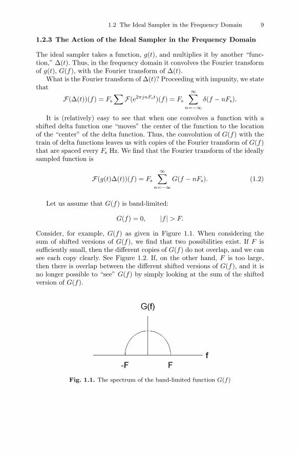
Let us assume that G(f) is band-limited:
G(f) = 0, |f | > F.
Consider, for example, G(f) as given in Figure 1.1. When considering thesum of shifted versions of G(f), we find that two possibilities exist. If F issufficiently small, then the different copies of G(f) do not overlap, and we cansee each copy clearly. See Figure 1.2. If, on the other hand, F is too large,then there is overlap between the different shifted versions of G(f), and it isno longer possible to “see” G(f) by simply looking at the sum of the shiftedversion of G(f).
Fig. 1.1. The spectrum of the band-limited function G(f)
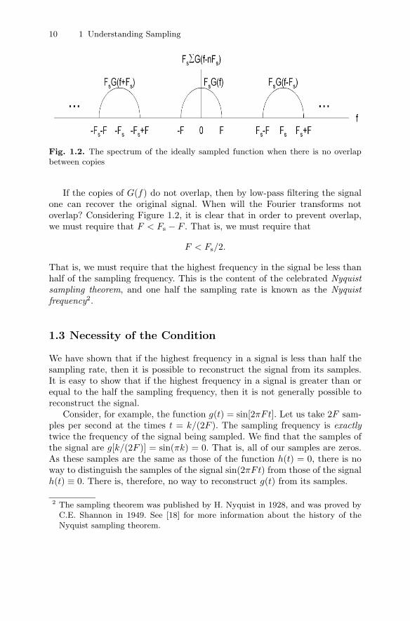
10 1 Understanding Sampling
Fig. 1.2. The spectrum of the ideally sampled function when there is no overlapbetween copies
If the copies of G(f) do not overlap, then by low-pass filtering the signalone can recover the original signal. When will the Fourier transforms notoverlap? Considering Figure 1.2, it is clear that in order to prevent overlap,we must require that F < Fs − F . That is, we must require that
F < Fs/2.
That is, we must require that the highest frequency in the signal be less thanhalf of the sampling frequency. This is the content of the celebrated Nyquistsampling theorem, and one half the sampling rate is known as the Nyquistfrequency2.
1.3 Necessity of the Condition
We have shown that if the highest frequency in a signal is less than half thesampling rate, then it is possible to reconstruct the signal from its samples.It is easy to show that if the highest frequency in a signal is greater than orequal to the half the sampling frequency, then it is not generally possible toreconstruct the signal.
Consider, for example, the function g(t) = sin[2πFt]. Let us take 2F sam-ples per second at the times t = k/(2F ). The sampling frequency is exactlytwice the frequency of the signal being sampled. We find that the samples ofthe signal are g[k/(2F )] = sin(πk) = 0. That is, all of our samples are zeros.As these samples are the same as those of the function h(t) = 0, there is noway to distinguish the samples of the signal sin(2πFt) from those of the signalh(t) ≡ 0. There is, therefore, no way to reconstruct g(t) from its samples.
2 The sampling theorem was published by H. Nyquist in 1928, and was proved byC.E. Shannon in 1949. See [18] for more information about the history of theNyquist sampling theorem.
1.6 The Net Effect 11
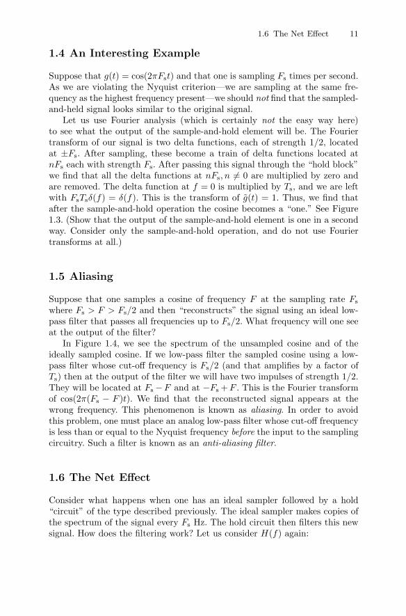
1.4 An Interesting Example
Suppose that g(t) = cos(2πFst) and that one is sampling Fs times per second.As we are violating the Nyquist criterion—we are sampling at the same fre-quency as the highest frequency present—we should not find that the sampled-and-held signal looks similar to the original signal.
Let us use Fourier analysis (which is certainly not the easy way here)to see what the output of the sample-and-hold element will be. The Fouriertransform of our signal is two delta functions, each of strength 1/2, locatedat ±Fs. After sampling, these become a train of delta functions located atnFs each with strength Fs. After passing this signal through the “hold block”we find that all the delta functions at nFs, n �= 0 are multiplied by zero andare removed. The delta function at f = 0 is multiplied by Ts, and we are leftwith FsTsδ(f) = δ(f). This is the transform of g(t) = 1. Thus, we find thatafter the sample-and-hold operation the cosine becomes a “one.” See Figure1.3. (Show that the output of the sample-and-hold element is one in a secondway. Consider only the sample-and-hold operation, and do not use Fouriertransforms at all.)
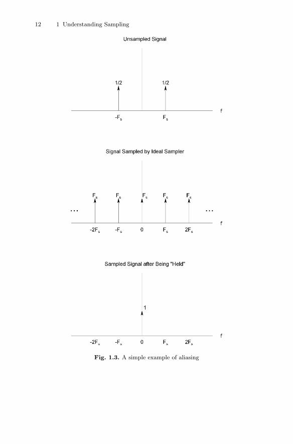
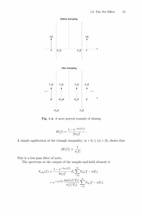
1.5 Aliasing
Suppose that one samples a cosine of frequency F at the sampling rate Fs
where Fs > F > Fs/2 and then “reconstructs” the signal using an ideal low-pass filter that passes all frequencies up to Fs/2. What frequency will one seeat the output of the filter?
In Figure 1.4, we see the spectrum of the unsampled cosine and of theideally sampled cosine. If we low-pass filter the sampled cosine using a low-pass filter whose cut-off frequency is Fs/2 (and that amplifies by a factor ofTs) then at the output of the filter we will have two impulses of strength 1/2.They will be located at Fs −F and at −Fs +F . This is the Fourier transformof cos(2π(Fs − F )t). We find that the reconstructed signal appears at thewrong frequency. This phenomenon is known as aliasing. In order to avoidthis problem, one must place an analog low-pass filter whose cut-off frequencyis less than or equal to the Nyquist frequency before the input to the samplingcircuitry. Such a filter is known as an anti-aliasing filter.
1.6 The Net Effect
Consider what happens when one has an ideal sampler followed by a hold“circuit” of the type described previously. The ideal sampler makes copies ofthe spectrum of the signal every Fs Hz. The hold circuit then filters this newsignal. How does the filtering work? Let us consider H(f) again:
12 1 Understanding Sampling
Fig. 1.3. A simple example of aliasing
1.6 The Net Effect 13
Fig. 1.4. A more general example of aliasing
H(f) =1 − e−2πjTsf
2πjf.
A simple application of the triangle inequality, |a + b| ≤ |a| + |b|, shows that
|H(f)| ≤ 1π|f | .
This is a low-pass filter of sorts.The spectrum at the output of the sample-and-hold element is
Vout(f) =1 − e−2πjfTs
2πjfFs
∞∑
−∞Vin(f − nFs)
= e−πjfTssin(πf/Fs)π(f/Fs)
∞∑
−∞Vin(f − nFs).
14 1 Understanding Sampling
For relatively small values of f we find that e−πjfTs and sin(πf/Fs)/(πf/Fs)are both near 1. When f is small we see that
Vout(f) ≈ Vin(f), |f | << Fs.
Let us consider how the rest of the copies of the spectrum are affected bythis filtering. At f = nFs, the sine term is zero. Thus, near multiples of thesampling frequency the contribution of the copies is small. In fact, as long asthe sampling frequency is much greater than the largest frequency in the signal,the contribution that the copies of the spectrum will make to the spectrum ofthe output of the sample-and-hold element will be small. If the sampling rateis not high enough, this is not true. See Exercise 7.
1.7 Undersampling
Suppose that one has a real signal all of whose energy is located between thefrequencies F1 and F2 (and −F2 and −F1) where F2 > F1. A naive applicationof the Nyquist sampling theorem would lead one to conclude that in order topreserve the information in the signal, one must sample the signal at a rateexceeding 2F2 samples per second. This, however, need not be so.
Consider the following example. Suppose that one has a signal whose en-ergy lies between 2 and 4 kHz (exclusive of the endpoints). If one samples thesignal at a rate of 4,000 sample per second, then one finds that the spectrumis copied into non-overlapping regions. Thus, after such sampling it is stillpossible to recover the signal. Sampling at a frequency that is less than theNyquist frequency is called undersampling . Generally speaking, in order to beable to reconstruct a signal from its samples, one must sample the signal at afrequency that exceeds twice the signal’s bandwidth.
1.8 The Experiment
1. Write a program for the ADuC841 that causes the microcontroller tosample a signal 1,000 times each second. Use channel 0 of the ADC forthe sampling operation.
2. Have the program move the samples from the ADC’s registers to theregisters that “feed” DAC 0. This will cause the samples to be output byDAC 0.
3. Connect a signal generator to the ADC and an oscilloscope to the DAC.4. Use a variety of inputs to the ADC. Make sure that some of the inputs
are well below the Nyquist frequency, that some are near the Nyquistfrequency, and that some exceed the Nyquist frequency. Record the oscil-loscope’s output.
1.10 Exercises 15
1.9 The Report
Make sure that your report includes the program you wrote, the plots thatyou captured, and an explanation of the extent to which your plots agree withthe theory described in this chapter.
1.10 Exercises
1. Suppose g(t) = sin(2πFst) and one uses a sample-and-hold element thatsamples at the times
t = nTs, n = 0, 1, . . . , Fs = 1/Ts.
Using Fourier transforms, calculate what the sampled-and-held waveformwill be.
2. Show that the frequency response of a filter whose impulse response is
h(t) ={
1 0 ≤ t < Ts
0 otherwise
is
H(f) =
{1−e−2πjfTs
2πjf f �= 0Ts f = 0
.
3. Show that H(f)—the frequency response of the “hold element”—can bewritten as
H(f) =
{e−jπTsf sin(πTsf)
πf f �= 0Ts f = 0
.
4. Let H(f) be given by the function
H(f) ={
1 2,200 < |f | < 2,8000 otherwise .
If one uses an ideal sampler to sample h(t) every Ts = 0.5ms, what willthe spectrum of the resulting signal be?
5. Show that the spectrum of an ideally sampled signal as given in (1.2) isperiodic in f and has period Fs.
6. Show that the function
f(t) =
{sin(π(2N+1)t)
sin(πt) t �= k
2N + 1 t = k
isa) Periodic with period 1.b) Continuous on the whole real line.
16 1 Understanding Sampling
Note that as both the numerator and the denominator are analytic func-tions and the quotient is continuous, the quotient must be analytic. (Thiscan be proved using Morera’s theorem [3, p. 133], for example.)
7. Construct a Simulink r© model that samples a signal 100 times per sec-ond and outputs the samples to an oscilloscope. Input a sinewave of fre-quency 5 Hz and one of frequency 49 Hz. You may use the “zero-orderhold” block to perform the sample-and-hold operation. Can you iden-tify the 5 Hz sinewave from its sampled version? What about the 49 Hzsinewave? Explain why the oscilloscope traces look the way they do.
2
Signal Reconstruction
Summary. We have seen that if one samples a signal at more than twice the highestfrequency contained in the signal, then it is possible, in principle, to reconstruct thesignal. In this chapter, we consider the reconstruction problem from a somewhatmore practical perspective.
Keywords. reconstruction, Taylor series.
2.1 Reconstruction
From what we described in Chapter 1, it would seem that all that one needsto do to reconstruct a signal is to apply an ideal low-pass filter—a low-passfilter whose frequency response is one up to the Nyquist frequency and zerofor all higher frequencies—to the sampled signal.
This is not quite true. Let us consider a practical sampling system—asystem in which the sample-and-hold element is a single element. In such asystem, one does not see perfect copies of the signal in the frequency domain.Such “pure copies” are found only when viewing an ideally sampled signal—asignal multiplied by a train of delta functions. As we saw in Chapter 1, thespectrum at the output of the sample-and-hold element is
Vout(f) = e−πjfTssin(πf/Fs)π(f/Fs)
∞∑
n=−∞Vin(f − nFs).
The sampling operation creates copies of the spectrum; the hold operationfilters all the copies somewhat. Even given an ideal low-pass filter that com-pletely removes all the copies of the spectrum centered at f = nFs, n �= 0, onefinds that the baseband copy of the spectrum, the copy centered at 0 Hz, is
Vlow-pass(f) = e−πjfTssin(πf/Fs)π(f/Fs)
Vin(f).
18 2 Signal Reconstruction
As we know [17] that
sin(x)/x ≈ 1 − x2/3, |x| << 1,
we find that if f is not too large, the magnitude of the Fourier transformof the low-passed version of the output of the sample-and-hold element isapproximately
|Vlow-pass(f)| ≈(
1 − (πf/Fs)2
3!
)|Vin(f)|.
If the sampling frequency is five times greater than the highest frequencypresent in the signal, then the highest frequency will be attenuated by afactor of approximately
attenuation ≈ 1 − (π/5)2/6 = 0.93.
That is, even after ideal filtering, the output of the sample-and-hold unit maybe attenuated by as much as 7%, and the degree of attenuation is frequency-dependent.
2.2 The Experiment
1. Build a Simulink r© system composed of a sinewave generator, a zero-orderhold element (which is equivalent to our sample-and-hold element), a high-order Butterworth filter, and an oscilloscope.
2. Set the zero-order hold to sample 100 times per second, and let the cut-offfrequency of the filter be 50 Hz.
3. Input signals that are well below, near, and above the Nyquist frequency.Record the input to, and the output of, the system.
2.3 The Report
In your report, include a description of the Simulink model built, a figure thatillustrates the system, and printouts of the oscilloscope input and output fora variety of frequencies.

2.4 Exercises 19
2.4 Exercises
1. By making use of the fact that the Taylor series that corresponds tosin(x)/x,
sin(x)x
= 1 − x2/3! + · · · + (−1)kx2k/(2k + 1)! + · · · ,
is an alternating series, prove that∣∣∣∣sin(x)
x− (1 − x2/3!)
∣∣∣∣ ≤1
120, |x| ≤ 1.
3
Time-limited Functions Are Not Band-limited
Summary. In this chapter, we show that it is impossible for both a function andits Fourier transform to be well localized. We show that if a function is compactlysupported—if it is zero outside of some bounded region—then its Fourier transformcannot be compactly supported. Then we show that the “narrower” a function is inthe time domain, the more spread out it will be in the frequency domain (and viceversa).
Keywords. compact support, analytic function, time-limited, band-limited, uncer-
tainty principle.
3.1 A Condition for Analyticity
The Fourier transform of a function, g(t), is
G(f) =∫ ∞
−∞e−2πjftg(t) dt.
Suppose that the function, g(t), is continuous and compactly supported—thatg(t) = 0 if |t| ≥ T . Then the Fourier transform of g(t), G(f), is equal to
G(f) =∫ T
−T
e−2πjftg(t) dt =∫ T
−T
∞∑
k=0
(−2πjft)k
k!g(t) dt.
We would like to interchange the order of integration and summation, so wemust show that the series converges uniformly. To this end, we consider theabsolute value of the terms
(−2πjft)k
k!g(t)
when |t| ≤ T . We find that
22 3 Time-limited Functions Are Not Band-limited
∣∣∣∣(−2πjft)k
k!g(t)∣∣∣∣ ≤
(2π|f |T )k
k!max|t|≤T
|g(t)|.
We now consider the remainder of the series appearing in the calculation ofG(f). We consider the sum
∞∑
k=N
(−2πjft)k
k!g(t).
We find that∣∣∣∣∣
∞∑
k=N
(−2πjft)k
k!g(t)
∣∣∣∣∣ ≤∞∑
k=N
∣∣∣∣(−2πjft)k
k!g(t)∣∣∣∣ ≤
∞∑
k=N
(2π|f |T )k
k!max|t|≤T
|g(t)|.
Considering the sum∞∑
k=N
Cxk
k!, x > 0,
we find that∞∑
k=N
Cxk
k!= C
xN
(N − 1)!
∞∑
k=N
xk−N
k(k − 1) · · ·N
≤ CxN
(N − 1)!
∞∑
k=N
xk−N
(k − N)!
=xN
(N − 1)!ex.
As N → ∞ this sum tends to zero. Applying this result to our sum, we findthat ∣∣∣∣∣
∞∑
k=N
(−2πjft)k
k!g(t)
∣∣∣∣∣ ≤ max|t|≤T
|g(t)| (2π|f |T )N
(N − 1)!e2π|f |T .
As N → ∞ this sum tends to zero uniformly in t, and the sum that appears inthe calculation of G(f) is uniformly convergent. This allows us to interchangethe order of summation and integration in the integral that defines G(f).Interchanging the order of summation and integration, we find that
G(f) =∞∑
k=0
fk (−2πj)k
k!
∫ T
−T
tkg(t) dt.
As G(f) is represented by a convergent Taylor series, it is analytic [3, p. 159].That is, the Fourier transform of a compactly supported function is analytic.(In order to show that the value of the remainder of the series tends to zerouniformly, we made use of the fact that g(t) is zero for |t| > T . When g(t) isnot time-limited, it is possible for G(f) to be band-limited.)
3.3 The Uncertainty Principle 23
3.2 Analyticity Implies Lack of Compact Support
It is well known and easy to prove that a non-constant analytic functioncannot be constant along any smooth curve [3, p. 284]. Thus, as long as G(f)is not identically zero, it cannot be zero on any interval. Thus, a non-zerotime-limited function—a non-zero function that is compactly supported intime—cannot be band-limited. The same basic proof shows that band-limitedfunctions cannot be time-limited. (See Exercise 1.)
3.3 The Uncertainty Principle
We now prove that a function cannot be well localized in time and frequency.We showed above that if a function is completely localized in time, it cannotbe completely localized in frequency. We now extend this result.
We prove that(∫ ∞
−∞t2|f(t)|2 dt/E
)(∫ ∞
−∞f2|F (f)|2 df/E
)≥ 1/(16π2) (3.1)
whereE ≡
∫ ∞
−∞|f(t)|2 dt
Parseval=∫ ∞
−∞|F (f)|2 df.
The normalized integrals in (3.1) measure the degree of localization of a func-tion and its Fourier transform. (See Exercise 3.) The bigger either number is,the less localized the relevant function is.
To prove (3.1), we consider the integral∫ ∞
−∞tf(t)
df(t)dt
dt.
The Cauchy-Schwarz inequality for integrals [18] shows that∣∣∣∣∫ ∞
−∞tf(t)
df(t)dt
dt
∣∣∣∣ ≤√∫ ∞
−∞t2|f(t)|2 dt
√∫ ∞
−∞
∣∣∣∣df(t)
dt
∣∣∣∣2
dt. (3.2)
Let us evaluate the leftmost integral. Making the (relatively mild) assump-tion that
lim|t|→∞
√|t|f(t) = 0,
we find that∫ ∞
−∞tf(t)
df(t)dt
dt =∫ ∞
−∞tdf2(t)/2
dtdt
= tf2(t)/2∣∣∞−∞ −
∫ ∞
−∞f2(t)/2 dt
= −∫ ∞
−∞f2(t)/2 dt.
24 3 Time-limited Functions Are Not Band-limited
Let us now evaluate the other integral of interest in (3.2). Making use ofParseval’s theorem [7] and the fact that the Fourier transform of the derivativeof a function is 2πjf times the Fourier transform of the original function, wefind that ∫ ∞
−∞
∣∣∣∣df(t)
dt
∣∣∣∣2
dt = (2π)2∫ ∞
−∞f2|F (f)|2 df.
Squaring both sides of (3.2) and combining all of our results, we find that(∫ ∞
−∞t2|f(t)|2 dt/E
)(∫ ∞
−∞f2|F (f)|2 df/E
)≥ 1/(16π2).
3.4 An Example
Let us consider the function g(t) = e−|t|. It is well known [7] that
G(f) =2
(2πf)2 + 1.
In this case,
E =∫ ∞
−∞
(e−|t|
)2
dt =∫ ∞
−∞e−2|t| dt = 1.
By making use of integration by parts twice, it is easy to show that∫ ∞
−∞t2e−2|t| dt =
12.
What remains is to calculate the integral∫ ∞
−∞
4f2
[(2πf)2 + 1]2df.
One way to calculate this integral is to make use of the method of residues.(For another method, see Exercise 6.)
Let CR be the boundary of the upper half-disk of radius R traversed incounter-clockwise direction. That is, we start the curve from −R, continuealong the real axis to +R, and then leave the real axis and traverse the uppersemicircle in the counter-clockwise direction. Because the order of the numer-ator is two greater than that of the denominator, it is easy to show that asR → ∞, the contribution of the semicircle tends to zero.
We find that∫ ∞
−∞
4f2
[(2πf)2 + 1]2df = 4 lim
R→∞
∮
CR
z2
[(2πz)2 + 1]2dz.
As long as R > 1, we find that inside the curve CR, the integrand has onepole of multiplicity 2 at the point z = −j/(2π). Rewriting the integrand as
3.5 The Best Function 25
z2
[(2πz)2 + 1]2=
1(2π)4
z2
[z + j/(2π)]2[z − j/(2π)]2,
it is clear that the residue at j/(2π) is
ddz
1(2π)4
z2
[z + j/(2π)]2
∣∣∣∣z=j/(2π)
=−jπ
21
(2π)4.
We find that for all R > 1,
4∮
CR
z2
[(2πz)2 + 1]2dz = 4 × 2πj ×−jπ
21
(2π)4=
14π2
.
In particular, we conclude that∫ ∞
−∞
4f2
[(2πf)2 + 1]2df =
14π2
.
All in all, we find that(∫ ∞
−∞t2|f(t)|2 dt/E
)(∫ ∞
−∞f2|F (f)|2 df/E
)=
18π2
>1
16π2.
This is in perfect agreement with the theory we have developed.
3.5 The Best Function
Which functions achieve the lower bound in (3.1)? In our proof, it is theCauchy-Schwarz inequality that leads us to the conclusion that the productis greater than or equal to 1/(16π2). In the proof of the Cauchy-Schwarzinequality (see, for example, [7]), it is shown that equality holds if the twofunctions whose squares appear in the inequality are constant multiples ofone another. In our case, this means that we must find the functions thatsatisfy
df(t)dt
= ctf(t).
It is easy to see (see Exercise 2) that the only functions that satisfy thisdifferential equation and that are square integrable1 are the functions
f(t) = Dect2/2, c < 0.
1 Square integrable functions are functions that satisfy∫∞−∞ |f(t)|2 dt < ∞.
26 3 Time-limited Functions Are Not Band-limited
3.6 Exercises
1. Prove that a non-constant band-limited function cannot be time-limited.2. Find the solutions of the equation
df
dt= ctf(t).
Show that the only solutions of this equation that are square integrable,that is, the only solutions, f(t), for which
∫ ∞
−∞f2(t) dt < ∞,
are the functionsf(t) = Dect2/2, c < 0.
3. Consider the functions
fW (t) =1√W
ΠW (t)
where the function ΠW (t) is defined as
ΠW (t) ≡{
1 |t| ≤ W/20 otherwise .
Show that
loc(W ) ≡(∫ ∞
−∞t2|fW (t)|2 dt/E
)
is a monotonically increasing function of W . Explain how this relates tothe fact that loc(W ) is a measure of the extent to which the functionsfW (t) are localized.
4. Letg(t) =
1√2π
e−t2/2.
Calculate G(f), and show that for this Gaussian function the two sides ofInequality (3.1) are actually equal. (One may use a table of integrals toevaluate the integrals that arise. Alternatively, one can make use of theproperties of the Gaussian PDF for this purpose.)
5. Explain why, if one makes use of the criterion of this chapter to determinehow localized a function is, it is reasonable to say that the function
f(t) ={
sin(t)t t �= 0
1 t = 0
is “totally unlocalized.”6. Let g(t) = e−|t| as it is in Section 3.4.
3.6 Exercises 27
a) Show that for this g(t),∫ ∞
−∞f2|G(f)|2 df =
∫ ∞
−∞f2G(f)2 df.
b) Calculate ∫ ∞
−∞f2G(f)2 df
by making use of Parseval’s theorem and the properties of the Fouriertransform. (You may ignore any “small” problems connected to dif-ferentiating g(t).)
4
Fourier Analysis and the Discrete FourierTransform
Summary. Having discussed sampling and time-limiting and how they affect asignal’s spectrum, we move on to the estimation of the spectrum of a signal fromthe signal’s samples. In this chapter, we introduce the discrete Fourier transform, wediscuss its significance, and we derive its properties. Then we discuss the family ofalgorithms know as fast Fourier transforms. We explain their significance, describehow one uses them, and discuss zero-padding and the fast convolution algorithm.
Keywords. Fourier transform, discrete Fourier transform, fast Fourier transform,
zero-padding, fast convolution.
4.1 An Introduction to the Discrete Fourier Transform
Often, we need to determine the spectral content of a signal—how much ofa signal’s power is located at a given frequency. In general, this means thatwe would like to determine the Fourier transform of the signal. Because weare actually measuring the signal, we cannot possibly know its values fromt = −∞ to t = +∞. We can only know the signal’s value in some finiteinterval. As we generally use a microprocessor to make measurements, evenin that interval we only know the signal’s value at discrete times—generallyat the times t = nTs where Ts is the sampling period. From this set of time-limited samples, we would like to estimate the Fourier transform of the signal.
If all that one knows of a signal is its value in an interval it is clearlyimpossible to determine the signal’s Fourier transform. Something must beassumed about the signal at the times for which no measurements exist. Afairly standard assumption, and the most reasonable in many ways, is that thefunction is zero outside the region in which it is measured and is reasonablysmooth inside this region. We will, once again, consider the consequencesof time-limiting the function—of “lopping off the tails” of the function—inChapter 5.
Recalling that the Fourier transform of a function, y(t), is
30 4 Fourier Analysis and the Discrete Fourier Transform
Y (f) = F(y(t))(f) ≡∫ ∞
−∞e−2πjfty(t) dt,
we find that given a function, y(t), which is zero outside the region t ∈ [0, T ],we can express its Fourier transform as
Y (f) =∫ T
0
e−2πjfty(t) dt.
Suppose that we have only N samples of the function taken at t = k(T/N), k =0, . . . , N − 1. Then we can estimate the integral by
Y (f) ≈N−1∑
k=0
e−2πjfkT/Ny(kT/N)(T/N).
If we specialize the frequencies we are interested in to f = m/T, n =0, . . . N − 1, then we find that
Y (m/T ) ≈ (T/N)N−1∑
k=0
e−2πjmk/Nyk, yk = y(kT/N). (4.1)
The discrete Fourier transform (DFT) of the sequence yk is defined as
Ym = DFT({yk})(m) ≡N−1∑
k=0
e−2πjmk/Nyk. (4.2)
The value of the DFT is (up to the constant of proportionality T/N) anapproximation of the value of the Fourier transform at the frequency m/T .
4.2 Two Sample Calculations
Consider the sequence {yk} given by
{−1, 1,−1, 1}.As N = 4, we find that
Y0 = e0(−1) + e0(1) + e0(−1) + e0(1) = 0Y1 = (e−πj/2)0(−1) + e−πj/2(1) + (e−πj/2)2(−1) + (e−πj/2)3(1)
= 1(−1) + (−j)(1) + (−1)(−1) + j(1) = 0Y2 = (−1)0(−1) + (−1)(1) + (−1)2(−1) + (−1)3(1) = −4Y3 = j0(−1) + j1(1) + j2(−1) + j3(1) = 0.
Now consider the sequence {zk} given by
4.3 Some Properties of the DFT 31
{1, 1, 0, 0}.
We find that
Zm =3∑
k=0
e−2πjkm/4yk =3∑
k=0
(e−jπ/2
)km
yk =3∑
k=0
(−j)kmyk.
Thus, we find that
Z0 = 2
Z1 =3∑
k=0
(−j)kyk = 1 − j
Z2 =3∑
k=0
(−j)2kyk =3∑
k=0
(−1)kyk = 0
Z3 =3∑
k=0
(−j)3kyk =3∑
k=0
jkyk = 1 + j.
4.3 Some Properties of the DFT
We have seen that the DFT is an approximation to the Fourier transform.Why use this particular approximation? The short answer is that the DFThas many nice properties, and many of the DFT’s properties “mimic” thoseof the Fourier transform.
The DFT, {Yk}, is an N -term sequence that is derived from another N -term sequence {yk}. We will shortly show that the mapping from sequence tosequence is invertible. Moreover, the mapping is almost an isometry—almostnorm-preserving. Let the l2 norm of an N -term sequence {c0, . . . cN−1} bedefined as √√√√
N−1∑
k=0
|ck|2.
Then the mapping preserves the l2 norm (except for multiplication by a con-stant) as well.
To show that the mapping is invertible, it is sufficient to produce an inversemapping. Consider the value of the sum
ak =N−1∑
m=0
e2πjkm/NYm.
We find that
32 4 Fourier Analysis and the Discrete Fourier Transform
ak =N−1∑
m=0
e2πjkm/NYm
=N−1∑
m=0
e2πjkm/NN−1∑
n=0
e−2πjmn/Nyn
=N−1∑
m=0
N−1∑
n=0
e−2πjmn/Ne2πjkm/Nyn
=N−1∑
n=0
yn
N−1∑
m=0
e−2πjm(n−k)/N .
As the inner sum is simply a geometric series, we can sum the series. We findthat for 0 ≤ n ≤ N − 1,
N−1∑
m=0
e−2πjm(n−k)/N =
{N, n = k
1−e2πj(n−k)
1−e−2πj(n−k)/N = 0, otherwise= Nδnk
where δnk = 1, n = k, and δnk = 0, n �= k. (The function δnk is known as theKronecker1 delta function.) We find that ak = Nyk. That is, we find that
yk = ak/N =1N
N−1∑
m=0
e+2πjkm/NYm.
This mapping of sequences is known as the inverse discrete Fourier transform(IDFT), and it is almost identical to the DFT.
In Section 4.2, we found that the DFT of the sequence {−1, 1,−1, 1} is
{Ym} = {0, 0,−4, 0}.Using the IDFT, we find that
y0 =14(−4) = −1
y1 =14
3∑
m=0
(eπj/2
)m
Ym =14(−1) · (−4) = 1
y2 =14
3∑
m=0
(eπj)m
Ym =141 · (−4) = −1
y3 =14
3∑
m=0
(e3πj/2
)m
Ym =14(−1) · (−4) = 1.
These are indeed the samples we started with in Section 4.2.1 Named after Leopold Kronecker (1823–1891) [18].
4.3 Some Properties of the DFT 33
Let
Y =
⎡
⎢⎣Y0
...YN−1
⎤
⎥⎦ and y =
⎡
⎢⎣y0
...yN−1
⎤
⎥⎦
where the elements of Y are the terms in the DFT of the sequence {y0, . . . , yN−1}.Consider the square of the norm of the vector, ‖Y‖2. We find that
‖Y‖2 ≡N−1∑
m=0
|Ym|2
=N−1∑
m=0
YmY m
=N−1∑
m=0
N−1∑
k=0
e2πjkm/Nyk
N−1∑
l=0
e−2πjlm/Nyl
=N−1∑
k=0
N−1∑
l=0
ykyl
N−1∑
m=0
e−2πj(k−l)m/N
=N−1∑
k=0
N−1∑
l=0
ykylNδkl
= NN−1∑
k=0
ykyk
= NN−1∑
k=0
|yk|2
= N‖y‖2.
We find that the mapping is almost an isometry. The mapping preserves thenorm up to a constant factor. Considering the transform pair {yk} ↔ {Ym}of Section 4.2, we find that ‖y‖2 = 4 and ‖Y‖2 = 16 = 4 · 4. This is in perfectagreement with the theory we have developed.
Assuming that the yk are real, we find that
YN−m =N−1∑
k=0
e−2πjk(N−m)/Nyk
=N−1∑
k=0
e−2πjk(−m)/Nyk
=N−1∑
k=0
e2πjkm/Nyk
34 4 Fourier Analysis and the Discrete Fourier Transform
=N−1∑
k=0
e−2πjkm/Nyk
= Ym.
This shows that |YN−m| = |Ym|. It also shows that when the yk are real, thevalues of Ym for m > N/2 do not contain any new information.
Consider the definition of the DFT:
Ym =N∑
k=0
e−2πjkm/Nyk.
Suppose that we allow m to be any integer—rather than restricting m to liebetween 0 and N − 1. Then we find that
YN+m =N∑
k=0
e−2πjk(N+m)/Nyk
=N∑
k=0
e−2πjkN/Nyke−2πjkm/Nyk
=N∑
k=0
e−2πjkm/Nyk.
That is, the “extended DFT,” {. . . , Y−1, Y0, Y1, . . .}, is periodic with periodN .
Finally, let us consider the DFT of the circular convolution (or cyclic con-volution) of two N -periodic sequences, ak and bk. Let the circular convolutionof the two sequence be defined as
yk = ak ∗ bk ≡N−1∑
n=0
anbk−n.
(As is customary, we denote the convolution operation by an asterisk.) Wefind that the DFT of yk is
Ym =N−1∑
k=0
e−2πjmk/Nyk
=N−1∑
k=0
e−2πjmk/NN−1∑
n=0
anbk−n
=N−1∑
n=0
an
N−1∑
k=0
e−2πjmk/Nbk−n
=N−1∑
n=0
e−2πjmn/Nan
N−1∑
k=0
e−2πjm(k−n)/Nbk−n.
4.4 The Fast Fourier Transform 35
As the sequence e−2πjm(k−n)/Nbk−n is periodic of period N in the variable k,the second sum above is simply the DFT of the sequence bk. The first sum isclearly the DFT of ak. Thus, we have shown that
Ym = AmBm. (4.3)
We have shown that the DFT of the circular convolution of two periodicsequences is the product of the DFTs of the two sequences.
4.4 The Fast Fourier Transform
The DFT can be used to approximate the Fourier transform. A practicalproblem with using the DFT is that calculating the DFT of a vector with Nelements seems to require N × N complex multiplications and (N − 1) × Ncomplex additions. Calculating the DFT seems to require approximately 2N2
arithmetical operations.In 1965, J.W. Cooley and J.W. Tukey published an important work [5]
in which they explained how under some conditions one could calculate anN -term DFT by performing on the order of N log(N) calculations2. As thelogarithm of N grows much slower than N , this made (and continues to make)the calculation of the DFT of large sequences possible. The algorithms relatedto this idea are known as fast Fourier transforms (FFTs).
To see how these algorithms work, consider a sequence with N terms, yk,k = 0, . . . N − 1, and let N be an even number. The sequence’s DFT is givenby
Ym =N−1∑
k=0
e−2πjkm/Nyk
=(N/2)−1∑
k=0
e−2πj(2k)m/Ny2k +(N/2)−1∑
k=0
e−2πj(2k+1)m/Ny2k+1
=(N/2)−1∑
k=0
e−2πjkm/(N/2)y2k + e−2πjm/N
(N/2)−1∑
k=0
e−2πjkm/(N/2)y2k+1.
We have calculated the DFT of yk by breaking up the N -term DFT into twoN/2-term DFTs. As each DFT takes approximately 2N2 terms, each of thesmaller DFTs requires approximately 2N2/4 operations. Since we have twoof the smaller DFTs to calculate, our total operation count is approximately2 The technique had been used in the past by such scientists as C.F. Gauss [18].
Until the advent of the computer, the technique was not very important. Cooleyand Tukey rediscovered the technique and appreciated its importance for digitalsignal processing.
36 4 Fourier Analysis and the Discrete Fourier Transform
N2. Additionally, the final reconstruction step requires N additions and Nmultiplications; it requires 2N arithmetical operations.
If we calculate the DFTs of the N/2-length sequences by splitting the se-quences, we will have four N/4-length DFTs to calculate. That will requireapproximately 4 · 2(N/4)2 = N2/2 calculations. In the reconstruction phase,we need 2 · 2N/2 = 2N additions and multiplications to reconstruct the twoN/2-length DFTs. We find that if we split the DFT twice, we need approxi-mately 2N2/22 + 2(2N) operations to calculate the original N sample DFT.In general, we find that if we split the dataset k times, we need approxi-mately 2N2/2k + k2N operations to calculate the original DFT. Supposingthat N = 2M , then if we perform M splits—the most we can perform—weneed approximately 2N2/2M +M2N = 2N +2 log2(N)N operations in orderto calculate the DFT of the original N -term sequence. As N is small relativeto N log(N), it is sufficient to say that FFT algorithm requires on the order ofN log(N) operations in order to calculate the DFT of an N -element sequence.
As the IDFT of a sequence is essentially the same as the DFT of thesequence, it is not surprising that there is also a fast inverse DFT known as theinverse fast Fourier transform (IFFT). The IFFT also requires on the order ofN log(N) operations to calculate the IDFT of an N -term sequence. The FFTalgorithm described above works properly only if the number of elements inthe sequence is a power of two. Generally speaking, FFT algorithms have arequirement that the number of elements must be of some specific form. (Inour case, the number of elements must be a power of two—but there are otheralgorithms, and they have different conditions.)
4.5 A Hand Calculation
Let us calculate the DFT of the sequence
{xn} = {−1, 1, 1, 1,−1, 0, 1, 0}
using the method of the previous section. We subdivide this large calculationinto two smaller calculations. We find that we must calculate the DFTs of thesequences
{−1, 1,−1, 1} and {1, 1, 0, 0}.The DFT of the first sequence is, as we have seen, {Ym} = {0, 0,−4, 0}. TheDFT of the second sequence is {Zm} = {2, 1 − j, 0, 1 + j}. According to ourrule, the final DFT must be
Xm = Ym + e−2πjm/NZm.
(In order to calculate values of Ym and Zm for m > 3, we make use of theperiodicity of the DFT and of the fact that all the samples are real numbers.)We find that
4.7 MATLAB, the DFT, and You 37
X0 = Y0 + Z0 = 2
X1 = Y1 + e−2πj/8Z1 =1 − j√
2(1 − j) = −j
√2
X2 = Y2 + e−2πj2/8Z2 = −4
X3 = Y3 + e−2πj3/8Z3 =−1 − j√
2(1 + j) = −j
√2
X4 = Y4 + e−2πj4/8Z4 = Y0 + e−2πj4/8Z0 = −2X5 = X8−3 = X3 = j
√2
X6 = X2 = −4X7 = X1 = j
√2.
4.6 Fast Convolution
In addition to the fact that the FFT makes it possible to calculate DFTs veryquickly, the FFT also enables us to calculate circular convolutions quickly. Letyn be the circular convolution of two N -periodic sequences, an and bn. Then,
yn = an ∗ bn =N−1∑
k=0
akbn−k, n = 0, . . . , N − 1.
In principle, each of the N elements of yn requires N multiplications andN − 1 additions. Thus, calculating the circular convolution seems to requireon the order of N2 calculations. As we saw previously (on p. 34), the DFTof the circular convolution of two sequences is the product of the DFTs ofthe sequences. Thus, it is possible to calculate the circular convolution bycalculating the DFTs of the sequences, calculating the product of the DFTs,and then calculating the IDFT of the resulting sequence. That is, we makeuse of the fact that
an ∗ bn = IDFT({DFT({an)}) element-wise× DFT({bn)})})
to calculate the circular convolution of two sequences. When performed in thisway by an FFT algorithm, the calculation requires on the order of N log(N)calculations, and not on the order of N2 calculations.
4.7 MATLAB, the DFT, and You
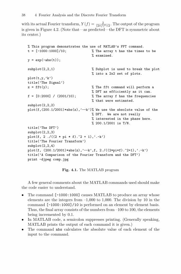
MATLAB r© has a command, fft, that calculates the DFT. The commandmakes use of an FFT algorithm whenever it can. Otherwise, it performs a“brute force” DFT. The fft command makes it very easy to calculate a DFT.The code segment of Figure 4.1 compares the DFT of the signal y(t) = e−|t|
38 4 Fourier Analysis and the Discrete Fourier Transform
with its actual Fourier transform, Y (f) = 2(2πf)2+2 . The output of the program
is given in Figure 4.2. (Note that—as predicted—the DFT is symmetric aboutits center.)
% This program demonstrates the use of MATLAB’s FFT command.
t = [-1000:1000]/10; % The array t has the times to be
% examined.
y = exp(-abs(t));
subplot(2,2,1) % Subplot is used to break the plot
% into a 2x2 set of plots.
plot(t,y,’k’)
title(’The Signal’)
z = fft(y); % The fft command will perform a
% DFT as efficiently as it can.
f = [0:2000] / (2001/10); % The array f has the frequencies
% that were estimated.
subplot(2,2,2)
plot(f,(200.1/2001)*abs(z),’--k’)% We use the absolute value of the
% DFT. We are not really
% interested in the phase here.
% 200.1/2001 is T/N.
title(’The DFT’)
subplot(2,2,3)
plot(f, 2 ./((2 * pi * f).^2 + 1),’.-k’)
title(’The Fourier Transform’)
subplot(2,2,4)
plot(f, (200.1/2001)*abs(z),’--k’,f, 2./((2*pi*f).^2+1),’.-k’)
title(’A Comparison of the Fourier Transform and the DFT’)
print -djpeg comp.jpg
Fig. 4.1. The MATLAB program
A few general comments about the MATLAB commands used should makethe code easier to understand.
• The command [-1000:1000] causes MATLAB to produce an array whoseelements are the integers from –1,000 to 1,000. The division by 10 in thecommand [-1000:1000]/10 is performed on an element by element basis.Thus, the final array consists of the numbers from –100 to 100, the elementsbeing incremented by 0.1.
• In MATLAB code, a semicolon suppresses printing. (Generally speaking,MATLAB prints the output of each command it is given.)
• The command abs calculates the absolute value of each element of theinput to the command.
4.8 Zero-padding and Calculating the Convolution 39
• The command subplot(m,n,k) causes MATLAB to create or refer to afigure with m × n subfigures. The next subfigure to be accessed will besubfigure k.
• The command plot(x,y) is used to produce plots. When used as shownabove—in its (almost) simplest form—the command plots the values of yagainst those of x.
• In the command plot(x,y,’--k’), the string ’--k’ tells MATLAB to usea black dashed line when producing the plot. (The string can be omittedentirely. When no control string is present, MATLAB uses its own defaultsto choose line styles and line colors.)
• The command title adds a title to the current plot.
MATLAB has several types of help commands, and all of them can be usedto learn more about these commands.
A few comments about the MATLAB code, and how it relates to what wehave seen about DFTs, are also in order. First of all, note that in the programthe value of the DFT returned by MATLAB is multiplied by 200.1/2,001. Thisis just T/N— the constant of proportionality from (4.1). (T = 200.1 because2,001 samples are taken and the time between samples is 0.1.)
The vector f is defined as f = [0:2000] / (2001/10);. That the vectormust contain 2,001 elements is clear. The data fed to the DFT had 2,001elements, and the length of the DFT is the same as that of the input data.The actual frequencies to which the elements of the DFT correspond arem/T, m = 0, . . . , 2,000. As T = 2,001/10, the division by 2,001/10 is ex-plained.
4.8 Zero-padding and Calculating the Convolution
Suppose that one would like to calculate the (ordinary) convolution of twonon-periodic sequences. That is, given {a0, . . . , aN−1} and {b0, . . . , bN−1}, onewould like to calculate
ck = ak ∗ bk ≡N−1∑
n=0
anbk−n, 0 ≤ k ≤ 2N − 2
where the value of an element of {ak} or {bk} whose index exceeds N − 1 oris less than 0 is taken to be zero.
One way to calculate this convolution is to calculate the given sum fork = 0, . . . , 2N − 2. This takes on the order of N2 operations. We have alreadyseen that for circular convolutions, this is not the best that one can do; here,too, one can do better.
Suppose that we almost double the length of each sequence by addingN − 1 zeros to the end of the sequence. That is, let us define the sequencesby taking
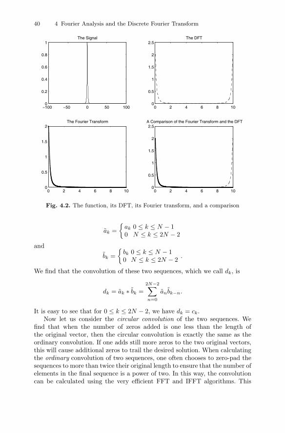
40 4 Fourier Analysis and the Discrete Fourier Transform
−100 −50 0 50 1000
0.2
0.4
0.6
0.8
1The Signal
0 2 4 6 8 100
0.5
1
1.5
2
2.5The DFT
0 2 4 6 8 100
0.5
1
1.5
2The Fourier Transform
0 2 4 6 8 100
0.5
1
1.5
2
2.5A Comparison of the Fourier Transform and the DFT
Fig. 4.2. The function, its DFT, its Fourier transform, and a comparison
ak ={
ak 0 ≤ k ≤ N − 10 N ≤ k ≤ 2N − 2
and
bk ={
bk 0 ≤ k ≤ N − 10 N ≤ k ≤ 2N − 2 .
We find that the convolution of these two sequences, which we call dk, is
dk = ak ∗ bk =2N−2∑
n=0
anbk−n.
It is easy to see that for 0 ≤ k ≤ 2N − 2, we have dk = ck.Now let us consider the circular convolution of the two sequences. We
find that when the number of zeros added is one less than the length ofthe original vector, then the circular convolution is exactly the same as theordinary convolution. If one adds still more zeros to the two original vectors,this will cause additional zeros to trail the desired solution. When calculatingthe ordinary convolution of two sequences, one often chooses to zero-pad thesequences to more than twice their original length to ensure that the number ofelements in the final sequence is a power of two. In this way, the convolutioncan be calculated using the very efficient FFT and IFFT algorithms. This
4.9 Other Perspectives on Zero-padding 41
allows us to calculate the convolution in on the order of N log(N) operations,rather than on the order of N2 operations.
Consider, for example, the convolution of the two ten-element sequences
{1, . . . , 1}, and {1, 2, . . . , 10}.
One way to perform this calculation is to extend both sequences to 32-elementsequences where the last 22 elements are all zero. One might give the followingcommands to MATLAB r© to define the sequences
a = [ones(size(1:10)) zeros(size(1:22))]b = [1:10 zeros(size(1:22))]
The first command produces a sequence with ten ones and 22 zeros. Thesecond produces a sequence composed of the numbers one through ten followedby 22 zeros. To calculate the convolution, one can give the command
ifft(fft(a) .* fft(b))
The .* command tells MATLAB to perform an element by element multi-plication on two sequences. The rest of the command causes MATLAB tocalculate the IFFT of the element by element product of the FFTs of thesequences a and b.
4.9 Other Perspectives on Zero-padding
We have seen one reason to zero-pad—it can allow one to calculate an (or-dinary) convolution using a circular convolution. There are two more reasonsone might want to zero-pad.
Suppose that one has samples, but the number of samples is not a power oftwo (or some other number of samples that makes using an FFT a possibility).Then one might choose to add samples in order to benefit from the efficiencyof the FFT.
Suppose that one adds zeros to a sequence of measurements that onehas made. When calculating the DFT of the “inflated” sequence one findsthat the maximum frequency of interest is still Fs/2—is still the Nyquistfrequency. What is changed is the number of frequency bands into which thefrequency band [0, Fs/2] is broken. When one zero-pads, one adds more pointsto the DFT. Thus, adding zeros in the time domain—zero-padding—leads tointerpolation in the spectral domain.
Sometimes, one adds zeros in order to perform this spectral interpolation.This is a third reason to zero-pad. Note that one has not gained informationby zero-padding—one is still calculating essentially the same approximationto the Fourier transform. One is approximating the Fourier transform at morefrequency points using the same time-limited, sampled signal.
42 4 Fourier Analysis and the Discrete Fourier Transform
4.10 MATLAB and the Serial Port
In order to use MATLAB to process data, one must transfer the data fromthe measurement instrument—in our case, the ADuC841—to MATLAB. Wewill do this by using the computer’s serial port—its UART. Using a serialport is very much like reading from, or writing to, a file. To set up and use aUART from MATLAB, one uses the commands serial, set, fopen, fprintf,fread, fclose, freeserial, and delete. Use the MATLAB help command(or the help window) to get more detail about how these commands are used.
4.11 The Experiment
In this laboratory, we build a system that measures the FFT of a signal moreor less on the fly. Use the ADuC841 to sample a signal, and then transmit themeasured values to MATLAB across a serial port. Have MATLAB take themeasured signal values, perform an FFT on them, and display the magnitudeof the FFT for the user.
In greater detail, write a program that causes the ADuC841 to sample2,000 times per second. Set up the ADuC841’s UART to transmit and receiveat 57,600 baud. Program the ADuC841 to transmit 512 measurements (1,024bytes) each time the UART receives the letter “s.”
Set up MATLAB to control the computer’s serial port. Have MATLABopen the serial port, write the letter “s” to it, and then receive the 1,024bytes. Once the measurements have been read in, reconstruct the signal mea-surements and have MATLAB calculate and display the absolute value of theFFT.
4.12 Exercises
1. Consider the following sequences• S1 ≡ {1, 0, 0, 0, 0},• S2 ≡ {1,−1, 1,−1}.a) Calculate the DFT of the sequences.b) Calculate the norms of the sequences and the transformed sequences.c) Compare the norms of the sequences and the transformed sequences,
and see if the results agree with the theory presented in the chapter.2. Why would it be inappropriate to speak of the FFT of the sequence S1 of
Exercise 1?3. Using the method of Sections 4.4 and 4.5 and the results of Exercise 1,
calculate the DFT of
{1, 1, 0,−1, 0, 1, 0,−1}.
4.12 Exercises 43
4. Note: you may wish to make use of [18] to gather the information necessaryto do this exercise.a) Give a brief description of the prime-factor algorithm (PFA).b) Historically, which came first—the Cooley-Tukey FFT or the PFA?
5. Using MATLAB, calculate the DFT of the sequence
sin(2πfnTs), n = 0, . . . , 255
for Ts = 1ms and f = 1, 10, 100, and 500 Hz. Plot the absolute value ofthe FFT against frequency. (Make sure that the frequency axis in the plotis defined in a reasonable way.) Explain what each plot “says” about thesignal.
6. Using MATLAB, calculate the DFT of the sequences e−knTs , n = 0, . . . 255for Ts = 10ms and k = 1, 2, 4, and 8. Plot the absolute value of the FFTagainst frequency. (Make sure that the frequency axis in the plot is definedin a reasonable way.)
7. Calculate the circular convolution of the sequence
an =
⎧⎨
⎩
0, n = 0, . . . , 501, n = 51, . . . , 2040, n = 205, . . . , 255
with itself by using the FFT and the IFFT. Plot the resulting samplesagainst their sample numbers. Submit the MATLAB code along with theanswer. (You may wish to make use of the MATLAB commands ones andzeros to help build up the initial vector.) Note that because of roundingerrors, the inverse discrete Fourier transform may have a very small imagi-nary component. This can lead the plotting routine supplied by MATLABto give odd results. You may wish to plot the value of the real part of theIDFT calculated by MATLAB. This can be achieved by using the realcommand provided by MATLAB.
8. Calculate the convolution of the two sequences
S1 ≡ {1, 2, . . . , k, . . . , 20}S2 ≡ {1, 4, . . . , k2, . . . , 400}
by zero-padding and using the MATLAB commands FFT and IFFT.9. Sample a 10 Hz sinewave at the times t = kTs, k = 0, . . . , 255 where the
sampling period is 10 ms.a) Calculate the FFT of this vector of 256 samples. Plot the absolute
value of the FFT against frequency. Make sure that the frequencyaxis is properly normalized.
b) Now, zero-pad the vector out to a length of 212 samples. Once again,plot the absolute value of the FFT against frequency. Make sure thatthe frequency axis is properly normalized.
c) Compare the results of the previous two sections, and explain thesimilarities and differences that you note.
5
Windowing
Summary. The DFT is an approximation to the Fourier transform of a signal. Theinput to the DFT is always a sequence of samples taken over a finite time period.This “truncation” of the signal changes the Fourier transform—the spectrum—ofthe signal. In this chapter, we learn about windowing; we learn how to control theeffect that truncation has on a signal’s spectrum.
Keywords. spectral leakage, sidelobes, windowing, Bartlett, Hann.
5.1 The Problems
By the nature of the way that we make measurements, we are always lookingat a finite-length sample of any signal. Let us define the function
ΠT (t) ≡{
1 |t| < T/20 |t| ≥ T/2 .
It is easy to show [7] that the Fourier transform of ΠT (t) is
F(ΠT (t))(f) =
{T f = 0T sin(πfT )
πfT f �= 0≡ T sinc(fT ). (5.1)
When considering a T second snippet of a signal s(t), one is essentiallyconsidering ΠT (t)s(t). From the standard properties of the Fourier transform,we find that
F(ΠT (t)s(t))(f) = S(f) ∗ [T sinc(fT )]
where the asterisk is once again used to represent the convolution operator.Consider what the result of this operation is when the signal is a cosine—
when s(t) = cos(2πFt). The Fourier transform of the signal is
S(f) = (1/2)[δ(f + F ) + δ(f − F )].
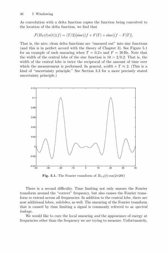
46 5 Windowing
As convolution with a delta function copies the function being convolved tothe location of the delta function, we find that
F(ΠT (t)s(t))(f) = (T/2)[sinc((f + F )T ) + sinc((f − F )T )].
That is, the nice, clean delta functions are “smeared out” into sinc functions(and this is in perfect accord with the theory of Chapter 3). See Figure 5.1for an example of such smearing when T = 0.2 s and F = 20Hz. Note thatthe width of the central lobe of the sinc function is 10 = 2/0.2. That is, thewidth of the central lobe is twice the reciprocal of the amount of time overwhich the measurement is performed. In general, width × T ≈ 2. (This is akind of “uncertainty principle.” See Section 3.3 for a more precisely stateduncertainty principle.)
−40 −30 −20 −10 0 10 20 30 40−0.04
−0.02
0
0.02
0.04
0.06
0.08
0.1
0.12
Fig. 5.1. The Fourier transform of Π0.2(t) cos(2π20t)
There is a second difficulty. Time limiting not only smears the Fouriertransform around the “correct” frequency, but also causes the Fourier trans-form to extend across all frequencies. In addition to the central lobe, there arenow additional lobes, sidelobes, as well. The smearing of the Fourier transformthat is caused by time limiting a signal is commonly referred to as spectralleakage.
We would like to cure the local smearing and the appearance of energy atfrequencies other than the frequency we are trying to measure. Unfortunately,
5.3 Some Standard Window Functions 47
we cannot take care of both problems at once. Generally speaking, what helpswith one problem exacerbates the other. Let us see why.
5.2 The Solutions
The Fourier transform of ΠT (t) decays relatively slowly—like 1/f . Why?Because ΠT (t) is not continuous. Discontinuous functions—functions withjumps—have a lot of energy at high frequencies. When one multiplies asignal—even a very smooth signal—by ΠT (t), one generally forces the func-tion to be discontinuous at the endpoints, t = ±T/2. This discontinuity isreflected in the signal’s Fourier transform by its slow decay. To take careof this problem, one must see to it that the sampled values approach zerocontinuously at the edges of the interval in which the measurement is beingmade.
Suppose that the function that one has measured is ΠT (t)s(t). How canone smooth the edges of this function? What one must do is multiply by asmooth function, w(t), whose support is located in the region t ∈ [−T/2, T/2]and for which w(T/2) = w(−T/2) = 0. Multiplying ΠT (t)s(t) by such afunction should get rid of some of the high-frequency energy that we sawpreviously. Of course a function that goes to zero smoothly inside this regionwill tend to emphasize the region near t = 0 more than it was emphasizedpreviously. One can consider this emphasis to be something that shrinks theeffective time over which the measurement was taken. As we have seen (inSection 3.3) that the shorter the time period over which the measurement istaken, the more spread out the Fourier transform of the resulting signal willbe, we must expect that after multiplication by w(t), the Fourier transform ofthe measured signal will have less energy at high frequencies—the sidelobeswill be smaller, but the Fourier transform will have a more smeared centrallobe.
The functions w(t) are known as window functions, and the process ofmultiplying the sampled function by a window function is known as windowingthe data. There are several standard window functions. Each function strikesa somewhat different balance between the width of the central lobe and therate at which the high-frequency component decays.
5.3 Some Standard Window Functions
We now present three standard window functions; there are many more. Whencharacterizing window functions, we consider:
1. The width of the central peak of the window function’s Fourier transform.The width is defined as the distance between the first zero to the left ofthe central peak and the first zero to the right of the central peak.
48 5 Windowing
2. The rate at which the sidelobes of the Fourier transform of the windowfunction decay.
5.3.1 The Rectangular Window
The window of the previous section, w(t) = ΠT (t), is called the rectangularwindow. Its Fourier transform is
F(ΠT (t))(f) = T sinc(fT ).
The first zero to the left of the central maximum occurs at f = −1/T , andthe first zero to the right of the central maximum occurs at f = 1/T . Thus,the width of the central lobe is 2/T . Additionally, as
|T sinc(fT )| =∣∣∣∣sin(πfT )
πf
∣∣∣∣ ≤1
π|f | ,
we find that the sidelobes decay like 1/f . Thus, the rectangular window hasa narrow main lobe, but its high-frequency terms decay slowly.
5.3.2 The Triangular Window
The triangle function is defined as
ΛT (t) =
⎧⎨
⎩
(t + T/2)/(T/2), −T/2 ≤ t ≤ 0(T/2 − t)/(T/2), 0 < t ≤ T/20, |t| > T/2
=2T
ΠT/2(t) ∗ ΠT/2(t).
As the Fourier transform of a convolution is the product of the Fourier trans-forms of the functions, by making use of (5.1) we find that
F(ΛT (t))(f) =2T
(T
2
)2
sinc2(fT/2) =T
2sinc2(fT/2).
As the first zeros of sinc(fT/2) are at f = ±2/T , the transform has a mainlobe that is twice as wide as the “unenhanced” window we used previously.However, the high-frequency terms decay like 1/f2 now.
The window based on this idea is known as the Bartlett window.
5.4 The Raised Cosine Window
Consider the function
w(t) = ΠT (t)(1 + cos(2πt/T )).
5.6 Applying a Window Function 49
At t = ±T/2, this function is not only continuous; it is once continuouslydifferentiable.
It is not hard to show (see Exercise 3) that the Fourier transform of thisfunction is
Tsinc(fT )1 − (fT )2
.
Note that there are zero-canceling poles at f = −1/T, 0, and f = 1/T . Thus,the zeros that bound the main lobe are located at f = ±2/T , and the widthof the main lobe is 4/T—just as it is for the Bartlett window. However, thedecay at high frequencies is 1/f3. Once again, we can trade a wide main lobefor rapid decay of high frequencies.
The window based on this idea is known as the Hann or Hanning window.(But note that MATLAB r© uses the names Hann and Hanning to define twoslightly different windows.) There are many other window functions. We willnot discuss them.
5.5 A Remark on Widths
We have defined the width of the main lobe to be the distance between thezeros of the main lobe. There are other ways of defining the width of themain lobe—and some of the other definitions distinguish between lobes moreeffectively than our simple definition.
5.6 Applying a Window Function
On a conceptual level, it is easiest to understand how windowing samplesaffects the spectral content of the sampled signal by considering multiply-ing the continuous-time signal by a continuous-time window. In practice, onegenerally samples the input signals “as is.” After sampling the signals, onemultiplies the samples by the relevant values of the window function. Thatis, rather than sampling x(t)w(t), one samples x(t), and then multiplies thesampled values x(nTs) by the samples of the window function, w(nTs).
MATLAB has predefined window functions like hann and bartlett. Thesefunctions take as their argument the number of samples to be windowed.Suppose that the MATLAB variable x has 256 unwindowed samples of asignal. If one would like to apply a raised cosine (Hann) window to the samplesand then calculate the FFT of the resulting sequence, one can give MATLABthe command
y = fft(x .* hann(256)’);
The “prime” (apostrophe) after the function call hann(256) takes the window“vector” and transposes it. This changes the window vector from a columnvector into a row vector. (Generally speaking, x is a row vector, and MATLAB
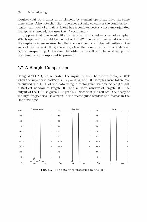
50 5 Windowing
requires that both items in an element by element operation have the samedimensions. Also note that the ’ operator actually calculates the complex con-jugate transpose of a matrix. If one has a complex vector whose unconjugatedtranspose is needed, one uses the .’ command.)
Suppose that one would like to zero-pad and window a set of samples.Which operation should be carried out first? The reason one windows a setof samples is to make sure that there are no “artificial” discontinuities at theends of the dataset. It is, therefore, clear that one must window a datasetbefore zero-padding. Otherwise, the added zeros will add the artificial jumpsthat windowing is supposed to prevent.
5.7 A Simple Comparison
Using MATLAB, we generated the input to, and the output from, a DFTwhen the input was cos(2π9.9t), Ts = 0.04, and 200 samples were taken. Wecalculated the DFT of the data using a rectangular window of length 200,a Bartlett window of length 200, and a Hann window of length 200. Theoutput of the DFT is given in Figure 5.2. Note that the roll-off—the decay ofthe high frequencies—is slowest in the rectangular window and fastest in theHann window.
0 10 200
10
20
30
40
50
60
70
80
90
100Rectangular
0 10 200
5
10
15
20
25
30
35
40
45
50Bartlett
0 10 200
5
10
15
20
25
30
35
40
45
50Hann
Fig. 5.2. The data after processing by the DFT
5.10 Exercises 51
5.8 MATLAB’s Window Visualization Tool
One nice way to “experience” the different windows is to use the MATLABwindow design and analysis tool. Open a MATLAB window, and type inwintool. From that point on, everything is self-explanatory.
5.9 The Experiment
Modify the programs written for the experiment of Chapter 4 to use severaldifferent window functions. It will probably be simplest to use the built-inwindow functions provided by MATLAB. Look up the commands bartlettand hann.
Write programs to use the Bartlett window, the Hann window, and at leastone window that has not been discussed in the text. Examine the output ofeach program when the input to the system is a sinewave. Explain the resultsin terms of the properties of the window function and the DFT.
5.10 Exercises
1. Use the definition of the Fourier transform to calculate the Fourier trans-form of ΠT (t).
2. Use the MATLAB wintool command to compare the Hann window andthe Hamming window.
3. Calculate the Fourier transform of the function
w(t) = ΠT (t)(1 + cos(2πt/T )).
4. Calculate the windowed DFT of the sequence sin(2πfnTs), n = 0, . . . , 255when f = 10 and Ts = 1ms, and plot the absolute value of the windowedDFT. Make use of:a) the rectangular window,b) the Bartlett window, andc) the Hanning window.
Compare the resulting DFTs.5. Calculate the DFT of the sequence
yk = sin(2π50kTs) + 0.01 sin(2π60kTs), k = 0, . . . , 1023, Ts = 1ms.
Plot the absolute value of the DFT (with a properly scaled frequencyaxis). Then recalculate the DFT using a 1,024-point Hanning window,and plot the absolute value of the resulting sequence (with a properlyscaled frequency axis). Explain the differences in the two plots.
6. Explain what apodization is and how it relates to windowing.
6
Signal Generation with the Help of MATLAB
Summary. One tool that an engineer often needs is a signal generator. Given amicroprocessor with a stable time-base and a nice size block of FLASH memory, itis easy to build a simple signal generator. In this very practically oriented chapter,we show how.
Keywords. signal generator, MATLAB, microprocessor.
6.1 Introduction
The ADuC841 has 64 kB of FLASH1 program memory from which the micro-processor can read while a program is executing. Our signal generator will beimplemented by storing the waveform we would like to output in the FLASHmemory and then using one of the ADuC841’s timers to control the speed atwhich the waveform is played back.
Of course, before we can play back a waveform, we must “record” it. Wewill make all of our “recordings” using MATLAB r©.
6.2 A Simple Sinewave Generator
Let us consider how we can “record” a sinewave in a way that will be usefulto us. It is our intention to play back our sinewave from the microprocessor’smemory.
MATLAB can be used to produce a vector with one full period of asinewave that has been sampled 256 times. The 256 samples are a good start.Next, the samples must be put in a form that is appropriate for the micropro-cessor. To do this, the samples must be output in hexadecimal, and they must1 FLASH memory is non-volatile memory that can be electrically erased and re-
programmed.
54 6 Signal Generation with the Help of MATLAB
correspond to positive voltages (as the ADuC841’s DAC converts to positivevoltages). Note that MATLAB has a command, dec2hex, that takes an inte-ger as input and produces a string whose characters are the hex digits thatcorrespond to the decimal number that was input. What we would ideally likeis to convert the vector of numbers into a set of instructions to the compilerthat will make the microprocessor store the values in a meaningful way.
It turns out that getting everything properly formatted is not hard. MAT-LAB has a command called fprintf that is very similar to the C commandof the same name. By using the MATLAB file commands and the fprintfcommand, one can cause MATLAB to output a file of the form
sine: DB 000HDB 00FH
.
.
.
This file can then be “pasted” into a program written in the ADuC841’sassembly language.
6.3 A Simple White Noise Generator
Not only can one use MATLAB to help write a sinewave generator, one canuse it to make a white noise generator. MATLAB has several commands forproducing white noise. The one that is most useful for our purposes is therand command. The rand(size([1:N])) command produces a vector thatis N elements long for which each element is (more or less) independent ofeach other element, and each element is a sample of a value from a randomvariable that is uniformly distributed over [0, 1]. Using fprintf, it is easy tocause MATLAB to generate a long list of (reasonably) uncorrelated numbers.
6.4 The Experiment
1. Cause MATLAB to generate 256 samples of a sinewave.2. Have MATLAB store the samples in a format that is appropriate for an
assembly language program.3. Write an assembly language program that reads the values of the sinewave
and outputs these values to DAC0.4. Write the program in such a way that the UART can be used to change
the frequency of the sinewave. (Have the program change the value(s) ofthe timer reload register(s) according to the value of the input from theUART.)
5. Examine the output of DAC0, and make sure that the period that is seencorresponds to the predicted period.
6.5 Exercises 55
6. Next, produce a set of 4,096 samples of random noise and incorporate thesevalues into a program that is similar to the program designed above.
7. Look at the spectrum of the signal produced in this way on an oscilloscopeoperating in FFT mode. What do you see?
6.5 Exercises
1. Define the term DCO. Please reference a source for the definition.2. In what way does the MATLAB command fprintf differ from C’s
fprintf command?
7
The Spectral Analysis of Random Signals
Summary. When one calculates the DFT of a sequence of measurements of arandom signal, one finds that the values of the elements of the DFT do not tendto “settle down” no matter how long a sequence one measures. In this chapter,we present a brief overview of the difficulties inherent in analyzing the spectra ofrandom signals, and we give a quick survey of a solution to the problem—the methodof averaged periodograms.
Keywords. random signals, method of averaged periodograms, power spectral den-
sity, spectral estimation.
7.1 The Problem
Suppose that one has N samples of a random signal1, Xk, k = 0, . . . , N−1, andsuppose that the samples are independent and identically distributed (IID).Additionally, assume that the random signal is zero-mean—that E(Xk) = 0.The expected value of an element of the DFT of the sequence, am, is
E(am) = E
(N−1∑
k=0
e−2πjkm/NXk
)= 0.
Because the signal is zero-mean, so are all of its Fourier coefficients. (All thisreally means is that the phases of the am are random, and the statisticalaverage of such am is zero.)
On the other hand, the power at a given frequency is (up to a constant ofproportionality) |am|2. The expected value of the power at a given frequency1 In this chapter, capital letters represent random variables, and lowercase letters
represent elements of the DFT of a random variable. As usual, the index k is usedfor samples and the index m for the elements of the DFT. In order to minimizeconfusion, we do not use the same letter for the elements of the sequence and forthe elements of its DFT.
58 7 The Spectral Analysis of Random Signals
is E(|am|2) and is non-negative. If one measures the value of |am|2 for someset of measurements, one is measuring the value of a random variable whoseexpected value is equal to the item of interest. One would expect that thelarger N was, the more certainly one would be able to say that the measuredvalue of |am|2 is near the theoretical expected value. One would be mistaken.
To see why, consider a0. We know that
a0 = X0 + · · · + XN−1.
Assuming that the Xk are real, we find that
|a0|2 =N−1∑
n=0
N−1∑
k=0
XnXk =N−1∑
n=0
X2k +
N−1∑
n=0
N−1,k �=n∑
k=0
XnXk.
Because the Xk are independent, zero-mean random variables, we know thatif n �= k, then E(XnXk) = 0. Thus, we see that the expected value of |a0|2 is
E(|a0|2) = NE(X2k). (7.1)
We would like to examine the variance of |a0|2. First, consider E(|a0|4).We find that
E(|a0|4) = NE(X4i ) + 3N(N − 1)E2(X2
i ).
(See Exercise 5 for a proof of this result.) Thus, the variance of the measure-ment is
E(|a0|4) − E2(|a0|2) = NE(X4i ) + 2N2E2(X2
i ) − 3NE2(X2i )
= Nσ2X2 + 2(N2 − N)E2(X2
i ).
Clearly, the variance of |a0|2 is O(N2), and the standard deviation of |a0|2 isO(N). That is, the standard deviation is of the same order as the measure-ment. This shows that taking larger values of N—taking more measurements—does not do much to reduce the uncertainty in our measurement of |a0|2. Infact, this problem exists for all the am, and it is also a problem when themeasured values, Xk, are not IID random variables.
7.2 The Solution
We have seen that the standard deviation of our measurement is of the sameorder as the expected value of the measurement. Suppose that rather thantaking one long measurement, one takes many smaller measurements. If themeasurements are independent and one then averages the measurements, thenthe variance of the average will decrease with the number of measurementswhile the expected value will remain the same.
Given a sequence of samples of a random signal, {X0, . . . , XN−1}, definethe periodograms, Pm, associated with the sequence by
7.3 Warm-up Experiment 59
Pm ≡ 1N
∣∣∣∣∣
N−1∑
k=0
e−2πjkm/NXk
∣∣∣∣∣
2
, m = 0, . . . , N − 1.
The value of the periodogram is the square of the absolute value of the mthelement of the DFT of the sequence divided by the number of elements in thesequence under consideration. The division by N removes the dependence thatthe size of the elements of the DFT would otherwise have on N—a dependencethat is seen clearly in (7.1).
The solution to the problem of the non-decreasing variance of the estimatesis to average many estimates of the same variable. In our case, it is convenientto average measurements of Pm, and this technique is known as the methodof averaged periodograms.
Consider the MATLAB r© program of Figure 7.1. In the program, MAT-LAB takes a set of 212 uncorrelated random numbers that are uniformly dis-tributed over (−1/2, 1/2), and estimates the power spectral density of the“signal” by making use of the method of averaged periodograms. The outputof the calculations is given in Figure 7.2. Note that the more sets the datawere split into, the less “noisy” the spectrum looks. Note too that the numberof elements in the spectrum decreases as we break up our data into smallersets. This happens because the number of points in the DFT decreases as thenumber of points in the individual datasets decreases.
It is easy to see what value the measurements ought to be approaching. Asthe samples are uncorrelated, their spectrum ought to be uniform. From thefact that the MATLAB-generated measurements are uniformly distributedover (−1/2, 1/2), it easy to see that
E(X2k) =
∫ 1/2
−1/2
α2 dα =α3
3
∣∣∣∣1/2
−1/2
=112
= 0.083.
Considering (7.1) and the definition of the periodogram, it is clear that thevalue of the averages of the 0th periodograms, P0, ought to be tending to 1/12.Considering Figure 7.2, we see that this is indeed what is happening—and themore sets the data are split into, the more clearly the value is visible. As thepower should be uniformly distributed among the frequencies, all the averagesshould be tending to this value—and this too is seen in the figure.
7.3 Warm-up Experiment
MATLAB has a command that calculates the average of many measurementsof the square of the coefficients of the DFT. The command is called psd (forpower spectral density). (See [7] for more information about the power spectraldensity.) The format of the psd command is psd(X,NFFT,Fs,WINDOW) (butnote that in MATLAB 7.4 this command is considered obsolete). Here, X is thedata whose PSD one would like to find, NFFT is the number of points in each
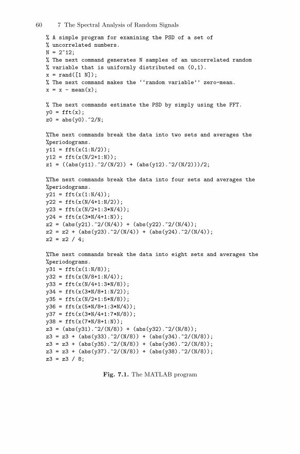
60 7 The Spectral Analysis of Random Signals
% A simple program for examining the PSD of a set of
% uncorrelated numbers.
N = 2^12;
% The next command generates N samples of an uncorrelated random
% variable that is uniformly distributed on (0,1).
x = rand([1 N]);
% The next command makes the ‘‘random variable’’ zero-mean.
x = x - mean(x);
% The next commands estimate the PSD by simply using the FFT.
y0 = fft(x);
z0 = abs(y0).^2/N;
%The next commands break the data into two sets and averages the
%periodograms.
y11 = fft(x(1:N/2));
y12 = fft(x(N/2+1:N));
z1 = ((abs(y11).^2/(N/2)) + (abs(y12).^2/(N/2)))/2;
%The next commands break the data into four sets and averages the
%periodograms.
y21 = fft(x(1:N/4));
y22 = fft(x(N/4+1:N/2));
y23 = fft(x(N/2+1:3*N/4));
y24 = fft(x(3*N/4+1:N));
z2 = (abs(y21).^2/(N/4)) + (abs(y22).^2/(N/4));
z2 = z2 + (abs(y23).^2/(N/4)) + (abs(y24).^2/(N/4));
z2 = z2 / 4;
%The next commands break the data into eight sets and averages the
%periodograms.
y31 = fft(x(1:N/8));
y32 = fft(x(N/8+1:N/4));
y33 = fft(x(N/4+1:3*N/8));
y34 = fft(x(3*N/8+1:N/2));
y35 = fft(x(N/2+1:5*N/8));
y36 = fft(x(5*N/8+1:3*N/4));
y37 = fft(x(3*N/4+1:7*N/8));
y38 = fft(x(7*N/8+1:N));
z3 = (abs(y31).^2/(N/8)) + (abs(y32).^2/(N/8));
z3 = z3 + (abs(y33).^2/(N/8)) + (abs(y34).^2/(N/8));
z3 = z3 + (abs(y35).^2/(N/8)) + (abs(y36).^2/(N/8));
z3 = z3 + (abs(y37).^2/(N/8)) + (abs(y38).^2/(N/8));
z3 = z3 / 8;
Fig. 7.1. The MATLAB program
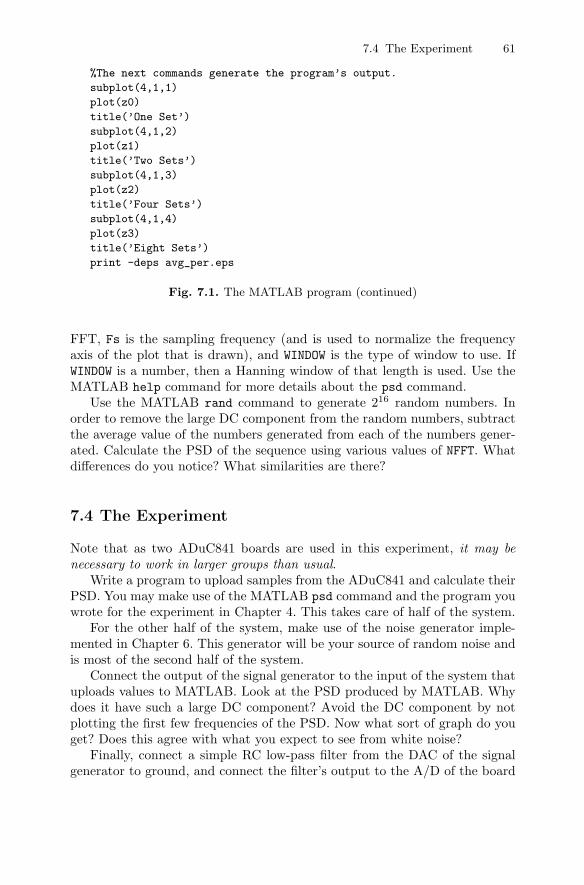
7.4 The Experiment 61
%The next commands generate the program’s output.
subplot(4,1,1)
plot(z0)
title(’One Set’)
subplot(4,1,2)
plot(z1)
title(’Two Sets’)
subplot(4,1,3)
plot(z2)
title(’Four Sets’)
subplot(4,1,4)
plot(z3)
title(’Eight Sets’)
print -deps avg_per.eps
Fig. 7.1. The MATLAB program (continued)
FFT, Fs is the sampling frequency (and is used to normalize the frequencyaxis of the plot that is drawn), and WINDOW is the type of window to use. IfWINDOW is a number, then a Hanning window of that length is used. Use theMATLAB help command for more details about the psd command.
Use the MATLAB rand command to generate 216 random numbers. Inorder to remove the large DC component from the random numbers, subtractthe average value of the numbers generated from each of the numbers gener-ated. Calculate the PSD of the sequence using various values of NFFT. Whatdifferences do you notice? What similarities are there?
7.4 The Experiment
Note that as two ADuC841 boards are used in this experiment, it may benecessary to work in larger groups than usual.
Write a program to upload samples from the ADuC841 and calculate theirPSD. You may make use of the MATLAB psd command and the program youwrote for the experiment in Chapter 4. This takes care of half of the system.
For the other half of the system, make use of the noise generator imple-mented in Chapter 6. This generator will be your source of random noise andis most of the second half of the system.
Connect the output of the signal generator to the input of the system thatuploads values to MATLAB. Look at the PSD produced by MATLAB. Whydoes it have such a large DC component? Avoid the DC component by notplotting the first few frequencies of the PSD. Now what sort of graph do youget? Does this agree with what you expect to see from white noise?
Finally, connect a simple RC low-pass filter from the DAC of the signalgenerator to ground, and connect the filter’s output to the A/D of the board
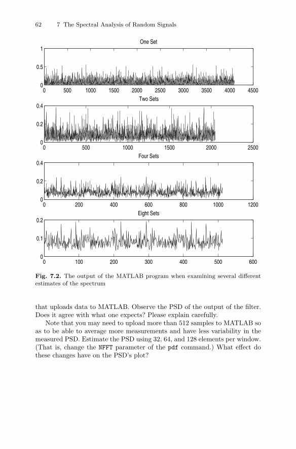
62 7 The Spectral Analysis of Random Signals
0 500 1000 1500 2000 2500 3000 3500 4000 45000
0.5
1One Set
0 500 1000 1500 2000 25000
0.2
0.4Two Sets
0 200 400 600 800 1000 12000
0.2
0.4Four Sets
0 100 200 300 400 500 6000
0.1
0.2Eight Sets
Fig. 7.2. The output of the MATLAB program when examining several differentestimates of the spectrum
that uploads data to MATLAB. Observe the PSD of the output of the filter.Does it agree with what one expects? Please explain carefully.
Note that you may need to upload more than 512 samples to MATLAB soas to be able to average more measurements and have less variability in themeasured PSD. Estimate the PSD using 32, 64, and 128 elements per window.(That is, change the NFFT parameter of the pdf command.) What effect dothese changes have on the PSD’s plot?
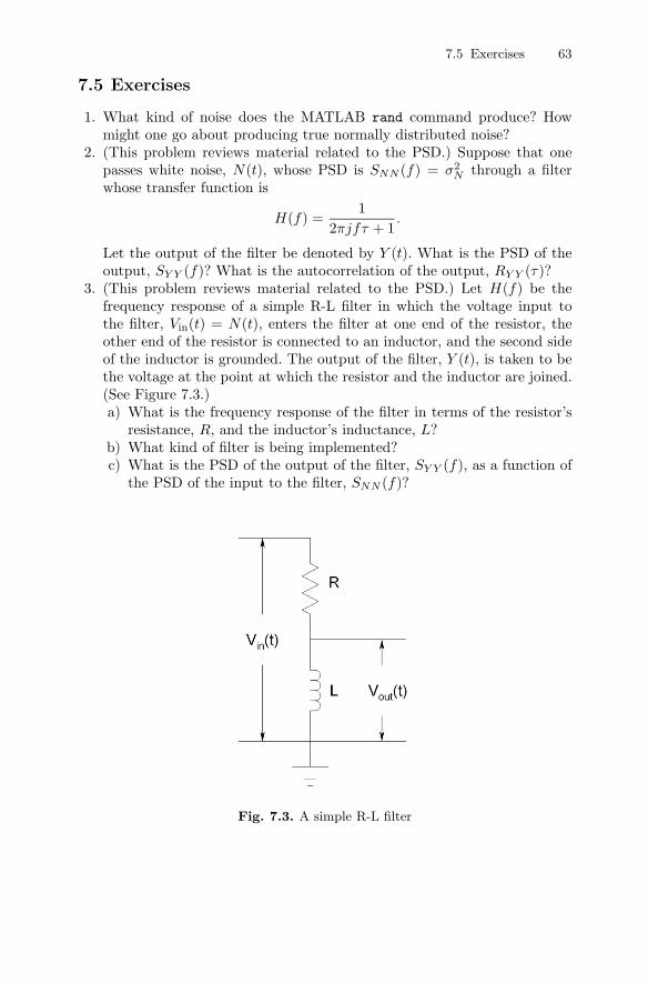
7.5 Exercises 63
7.5 Exercises
1. What kind of noise does the MATLAB rand command produce? Howmight one go about producing true normally distributed noise?
2. (This problem reviews material related to the PSD.) Suppose that onepasses white noise, N(t), whose PSD is SNN (f) = σ2
N through a filterwhose transfer function is
H(f) =1
2πjfτ + 1.
Let the output of the filter be denoted by Y (t). What is the PSD of theoutput, SY Y (f)? What is the autocorrelation of the output, RY Y (τ)?
3. (This problem reviews material related to the PSD.) Let H(f) be thefrequency response of a simple R-L filter in which the voltage input tothe filter, Vin(t) = N(t), enters the filter at one end of the resistor, theother end of the resistor is connected to an inductor, and the second sideof the inductor is grounded. The output of the filter, Y (t), is taken to bethe voltage at the point at which the resistor and the inductor are joined.(See Figure 7.3.)a) What is the frequency response of the filter in terms of the resistor’s
resistance, R, and the inductor’s inductance, L?b) What kind of filter is being implemented?c) What is the PSD of the output of the filter, SY Y (f), as a function of
the PSD of the input to the filter, SNN (f)?
Fig. 7.3. A simple R-L filter
64 7 The Spectral Analysis of Random Signals
4. Using Simulink r©, simulate a system whose transfer function is
H(s) =s
s2 + s + 10,000.
Let the input to the system be band-limited white noise whose bandwidthis substantially larger than that of the filter. Use a “To Workspace” blockto send the output of the filter to MATLAB. Use the PSD function to calcu-late the PSD of the output. Plot the PSD of the output against frequency.Show that the measured bandwidth of the output is in reasonable accordwith what the theory predicts. (Remember that the PSD is proportionalto the power at the given frequency, and not to the voltage.)
5. Let the random variables X0, . . . , XN−1 be independent and zero-mean.Consider the product
(X0 + · · ·+XN−1)(X0 + · · ·+XN−1)(X0 + · · ·+XN−1)(X0 + · · ·+XN−1).
a) Show that the only terms in this product that are not zero-mean areof the form X4
k or X2kX2
n, n �= k.b) Note that in expanding the product, each term of the form X4
k appearsonly once.
c) Using combinatorial arguments, show that each term of the form
X2kX2
n appears(
42
)times.
d) Combine the above results to conclude that (as long as the samplesare real)
E(|a0|4) = NE(X4k) + 6
N(N − 1)2
E2(X2k).

Part II
Analog to Digital and Digital to AnalogConverters
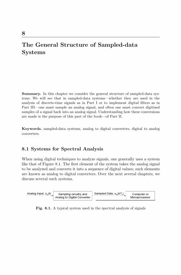
8
The General Structure of Sampled-dataSystems
Summary. In this chapter we consider the general structure of sampled-data sys-tems. We will see that in sampled-data systems—whether they are used in theanalysis of discrete-time signals as in Part I or to implement digital filters as inPart III—one must sample an analog signal, and often one must convert digitizedsamples of a signal back into an analog signal. Understanding how these conversionsare made is the purpose of this part of the book—of Part II.
Keywords. sampled-data systems, analog to digital converters, digital to analog
converters.
8.1 Systems for Spectral Analysis
When using digital techniques to analyze signals, one generally uses a systemlike that of Figure 8.1. The first element of the system takes the analog signalto be analyzed and converts it into a sequence of digital values; such elementsare known as analog to digital converters. Over the next several chapters, wediscuss several such systems.
Fig. 8.1. A typical system used in the spectral analysis of signals
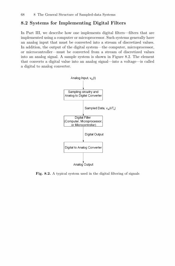
68 8 The General Structure of Sampled-data Systems
8.2 Systems for Implementing Digital Filters
In Part III, we describe how one implements digital filters—filters that areimplemented using a computer or microprocessor. Such systems generally havean analog input that must be converted into a stream of discretized values.In addition, the output of the digital system—the computer, microprocessor,or microcontroller—must be converted from a stream of discretized valuesinto an analog signal. A sample system is shown in Figure 8.2. The elementthat converts a digital value into an analog signal—into a voltage—is calleda digital to analog converter.
Fig. 8.2. A typical system used in the digital filtering of signals
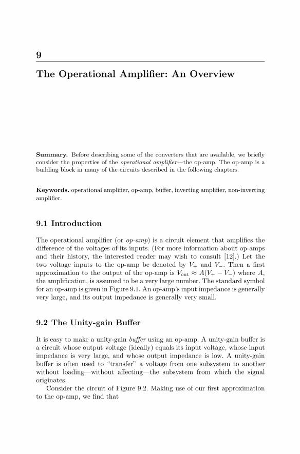
9
The Operational Amplifier: An Overview
Summary. Before describing some of the converters that are available, we brieflyconsider the properties of the operational amplifier—the op-amp. The op-amp is abuilding block in many of the circuits described in the following chapters.
Keywords. operational amplifier, op-amp, buffer, inverting amplifier, non-inverting
amplifier.
9.1 Introduction
The operational amplifier (or op-amp) is a circuit element that amplifies thedifference of the voltages of its inputs. (For more information about op-ampsand their history, the interested reader may wish to consult [12].) Let thetwo voltage inputs to the op-amp be denoted by V+ and V−. Then a firstapproximation to the output of the op-amp is Vout ≈ A(V+ − V−) where A,the amplification, is assumed to be a very large number. The standard symbolfor an op-amp is given in Figure 9.1. An op-amp’s input impedance is generallyvery large, and its output impedance is generally very small.
9.2 The Unity-gain Buffer
It is easy to make a unity-gain buffer using an op-amp. A unity-gain buffer isa circuit whose output voltage (ideally) equals its input voltage, whose inputimpedance is very large, and whose output impedance is low. A unity-gainbuffer is often used to “transfer” a voltage from one subsystem to anotherwithout loading—without affecting—the subsystem from which the signaloriginates.
Consider the circuit of Figure 9.2. Making use of our first approximationto the op-amp, we find that
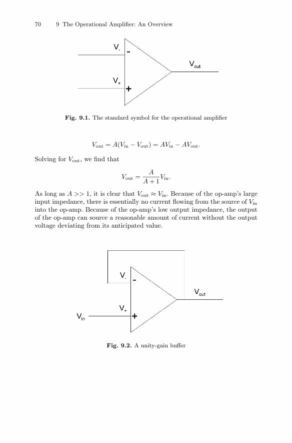
70 9 The Operational Amplifier: An Overview
Fig. 9.1. The standard symbol for the operational amplifier
Vout = A(Vin − Vout) = AVin − AVout.
Solving for Vout, we find that
Vout =A
A + 1Vin.
As long as A >> 1, it is clear that Vout ≈ Vin. Because of the op-amp’s largeinput impedance, there is essentially no current flowing from the source of Vin
into the op-amp. Because of the op-amp’s low output impedance, the outputof the op-amp can source a reasonable amount of current without the outputvoltage deviating from its anticipated value.
Fig. 9.2. A unity-gain buffer
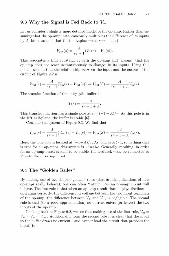
9.4 The “Golden Rules” 71
9.3 Why the Signal is Fed Back to V−
Let us consider a slightly more detailed model of the op-amp. Rather than as-suming that the op-amp instantaneously multiplies the difference of its inputsby A, let us assume that (in the Laplace—the s—domain)
Vout(s) =A
sτ + 1(V+(s) − V−(s)).
This associates a time constant, τ , with the op-amp and “means” that theop-amp does not react instantaneously to changes in its inputs. Using thismodel, we find that the relationship between the input and the output of thecircuit of Figure 9.2 is
Vout(s) =A
sτ + 1(Vin(s) − Vout(s)) ⇒ Vout(S) =
A
sτ + 1 + AVin(s).
The transfer function of the unity-gain buffer is
T (s) =A
sτ + 1 + A.
This transfer function has a single pole at s = (−1 − A)/τ . As this pole is inthe left half-plane, the buffer is stable [6].
Consider the system of Figure 9.3. We find that
Vout(s) =A
sτ + 1(Vout(s) − Vin(s)) ⇒ Vout(S) =
−A
sτ + 1 − AVin(s).
Here, the lone pole is located at (−1+A)/τ . As long as A > 1, something thatis true for all op-amps, this system is unstable. Generally speaking, in orderfor an op-amp-based system to be stable, the feedback must be connected toV−—to the inverting input.
9.4 The “Golden Rules”
By making use of two simple “golden” rules (that are simplifications of howop-amps really behave), one can often “intuit” how an op-amp circuit willbehave. The first rule is that when an op-amp circuit that employs feedback isoperating correctly, the difference in voltage between the two input terminalsof the op-amp, the difference between V+ and V−, is negligible. The secondrule is that (to a good approximation) no current enters (or leaves) the twoinputs of the op-amp.
Looking back at Figure 9.2, we see that making use of the first rule, Vin =V+ = V− = Vout. Additionally, from the second rule it is clear that the inputto the buffer draws no current—and cannot load the circuit that provides theinput, Vin.
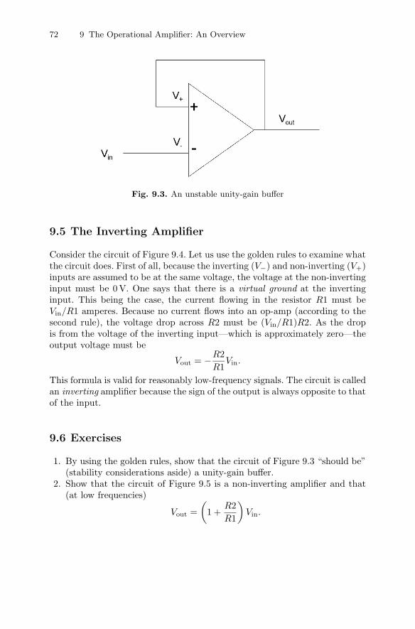
72 9 The Operational Amplifier: An Overview
Fig. 9.3. An unstable unity-gain buffer
9.5 The Inverting Amplifier
Consider the circuit of Figure 9.4. Let us use the golden rules to examine whatthe circuit does. First of all, because the inverting (V−) and non-inverting (V+)inputs are assumed to be at the same voltage, the voltage at the non-invertinginput must be 0 V. One says that there is a virtual ground at the invertinginput. This being the case, the current flowing in the resistor R1 must beVin/R1 amperes. Because no current flows into an op-amp (according to thesecond rule), the voltage drop across R2 must be (Vin/R1)R2. As the dropis from the voltage of the inverting input—which is approximately zero—theoutput voltage must be
Vout = −R2R1
Vin.
This formula is valid for reasonably low-frequency signals. The circuit is calledan inverting amplifier because the sign of the output is always opposite to thatof the input.
9.6 Exercises
1. By using the golden rules, show that the circuit of Figure 9.3 “should be”(stability considerations aside) a unity-gain buffer.
2. Show that the circuit of Figure 9.5 is a non-inverting amplifier and that(at low frequencies)
Vout =(
1 +R2R1
)Vin.
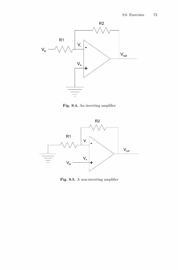
9.6 Exercises 73
Fig. 9.4. An inverting amplifier
Fig. 9.5. A non-inverting amplifier
10
A Simple Digital to Analog Converter
Summary. There are many ways of implementing digital to analog converters(D/As or DACs)—circuits that take an input that consists of “ones” and “zeros” andconvert the inputs into an analog output signal. (Often the “ones” are a referencevoltage, Vref and the “zeros” are 0 V.) In this chapter, we present one simple, albeitnot very practical, DAC. This DAC can be used with many types of microprocessorsand can be considered a purely passive DAC.
Keywords. digital to analog converter, DAC, passive DAC, buffer.
10.1 The Digital to Analog Converter
Consider the circuit of Figure 10.1. Let the inputs, b0, b1, and b2 be either0 V or Vref . Let us consider the output of the circuit when b2 = Vref , and letb1 = b0 = 0V. Then, we can redraw the circuit as shown in Figure 10.2.
Let us determine the output of the circuit in the second form. The resis-tance of the two resistors in parallel is
Resistance =1
12R + 1
4R
=4R
3.
As this resistor is in series with the R ohm resistor, the output of the circuitis
Vout =4R3
R + 4R3
Vref =47Vref .
Similar logic shows that if b0 = b2 = 0, b1 = Vref , then Vout = (2/7)Vref ,and if b1 = b2 = 0, b0 = Vref , then Vout = (1/7)Vref .
The principle of superposition states that, given a linear circuit, if a setof inputs I1 leads to the output O1, and if a second set of inputs I2 leads tothe output O2, then if one uses a1I1 + a2I2 as the input to the system, thenthe output of the system will be a1O1 + a2O2. The principle of superposition
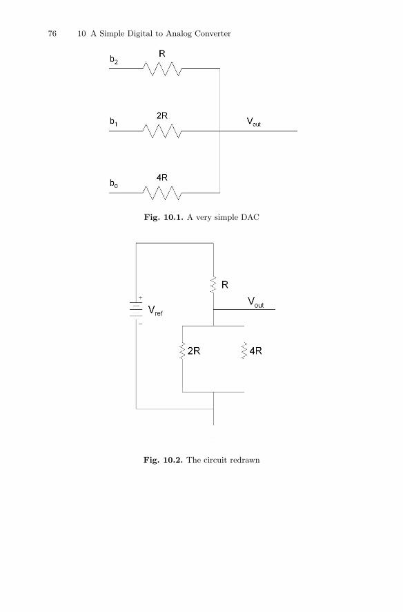
76 10 A Simple Digital to Analog Converter
Fig. 10.1. A very simple DAC
Fig. 10.2. The circuit redrawn
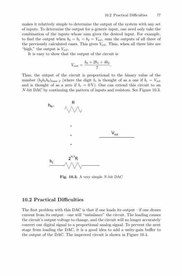
10.2 Practical Difficulties 77
makes it relatively simple to determine the output of the system with any setof inputs. To determine the output for a generic input, one need only take thecombination of the inputs whose sum gives the desired input. For example,to find the output when b0 = b1 = b2 = Vref , sum the outputs of all three ofthe previously calculated cases. This gives Vref . Thus, when all three bits are“high,” the output is Vref .
It is easy to show that the output of the circuit is
Vout =b0 + 2b1 + 4b2
7.
Thus, the output of the circuit is proportional to the binary value of thenumber (b2b1b0)base 2 (where the digit bi is thought of as a one if bi = Vref
and is thought of as a zero if bi = 0V). One can extend this circuit to anN -bit DAC by continuing the pattern of inputs and resistors. See Figure 10.3.
Fig. 10.3. A very simple N -bit DAC
10.2 Practical Difficulties
The first problem with this DAC is that if one loads its output—if one drawscurrent from its output—one will “unbalance” the circuit. The loading causesthe circuit’s output voltage to change, and the circuit will no longer accuratelyconvert our digital signal to a proportional analog signal. To prevent the nextstage from loading the DAC, it is a good idea to add a unity-gain buffer tothe output of the DAC. The improved circuit is shown in Figure 10.4.
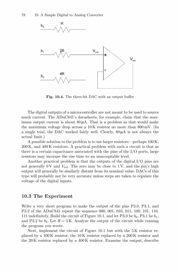
78 10 A Simple Digital to Analog Converter
Fig. 10.4. The three-bit DAC with an output buffer
The digital outputs of a microcontroller are not meant to be used to sourcemuch current. The ADuC841’s datasheets, for example, claim that the max-imum output current is about 80μA. That is a problem as that would makethe maximum voltage drop across a 10 K resistor no more than 800 mV. (Ina single trial, the DAC worked fairly well. Clearly, 80μA is not always theactual limit.)
A possible solution to the problem is to use larger resistors—perhaps 100 K,200 K, and 400 K resistors. A practical problem with such a circuit is that asthere is a certain capacitance associated with the pins of the I/O ports, largeresistors may increase the rise time to an unacceptable level.
Another practical problem is that the outputs of the digital I/O pins arenot generally 0 V and Vref . The zero may be close to 1 V, and the pin’s highoutput will generally be similarly distant from its nominal value. DACs of thistype will probably not be very accurate unless steps are taken to regulate thevoltage of the digital inputs.
10.3 The Experiment
Write a very short program to make the output of the pins P3.0, P3.1, andP3.2 of the ADuC841 repeat the sequence 000, 001, 010, 011, 100, 101, 110,111 indefinitely. Build the circuit of Figure 10.1, and let P3.0 be b0, P3.1 be b1,and P3.2 be b2. Let R = 5K. Analyze the output of the circuit while runningthe program you wrote.
Next, implement the circuit of Figure 10.1 but with the 5K resistor re-placed by a 100 K resistor, the 10 K resistor replaced by a 200 K resistor andthe 20 K resistor replaced by a 400 K resistor. Examine the output, describe

10.4 Exercises 79
how it differs from the output of the previous circuit, and explain why thedifferences you have observed exist. Please pay particular attention to thevoltage levels and the apparent rise time of the output.
10.4 Exercises
1. What simple additions could one make to the circuit of Figure 10.1 torid oneself of the problem of the circuit loading the ADuC841’s digitaloutputs? (Please keep your answer very simple.)
11
The Binary Weighted DAC
Summary. In the previous chapter, we considered a simple, entirely passive DAC.In this chapter, we consider the binary weighted DAC. This DAC is also very simplebut makes use of an op-amp in a way that is fundamental to the DAC’s performance.
Keywords. binary weighted DAC, op-amp.
11.1 The General Theory
The circuit of Figure 11.1 shows an N -bit binary weighted DAC. The DAC’sname comes from the way the resistors have been chosen; each resistor is twiceas large as the preceding resistor. This is a very simple DAC that makes useof an op-amp in a way that is fundamental to the DAC’s operation.
In Figure 11.1, the non-inverting input, V+, is tied to ground. Accordingto the golden rules, the voltage at the inverting input must be approximately0 V as well. That is why there is a dashed ground symbol at the inverting input.
The current in the branch to which bi is an input will be bi/(2(N−1)−iR).Because (according to the golden rules) no current enters the op-amp, thetotal current passing through the R ohm resistor sitting “above” the op-ampis
total current =N−1∑
i=0
bi
2(N−1)−iR=
12N−1R
N−1∑
i=0
2ibi.
The voltage at the output is the voltage that drops across the R ohm resistoris positioned above the op-amp. As this voltage drops from zero—from thevirtual ground—we find that the voltage at the output is
Vout = − 12N−1
N−1∑
i=0
2ibi.
Clearly, this voltage is proportional to the binary value of the word bN−1 · · · b0.
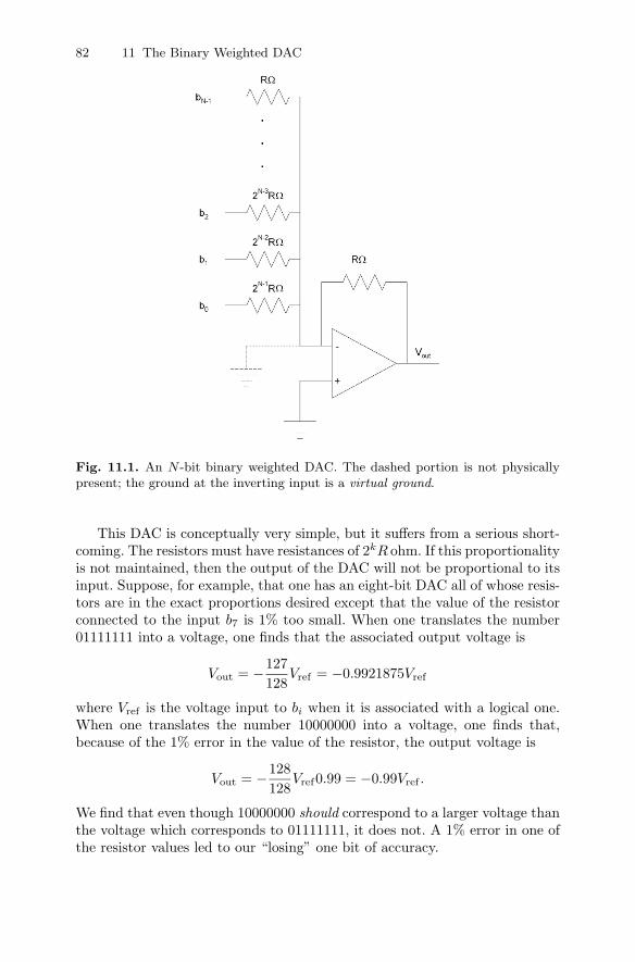
82 11 The Binary Weighted DAC
Fig. 11.1. An N -bit binary weighted DAC. The dashed portion is not physicallypresent; the ground at the inverting input is a virtual ground.
This DAC is conceptually very simple, but it suffers from a serious short-coming. The resistors must have resistances of 2kR ohm. If this proportionalityis not maintained, then the output of the DAC will not be proportional to itsinput. Suppose, for example, that one has an eight-bit DAC all of whose resis-tors are in the exact proportions desired except that the value of the resistorconnected to the input b7 is 1% too small. When one translates the number01111111 into a voltage, one finds that the associated output voltage is
Vout = −127128
Vref = −0.9921875Vref
where Vref is the voltage input to bi when it is associated with a logical one.When one translates the number 10000000 into a voltage, one finds that,because of the 1% error in the value of the resistor, the output voltage is
Vout = −128128
Vref0.99 = −0.99Vref .
We find that even though 10000000 should correspond to a larger voltage thanthe voltage which corresponds to 01111111, it does not. A 1% error in one ofthe resistor values led to our “losing” one bit of accuracy.

11.2 Exercises 83
Because of the need for accuracy in the various resistor values called forby the binary weighted DAC, such DACs generally have eight or fewer bits ofaccuracy.
11.2 Exercises
1. What accuracy is required of the resistor connected to b15 in a 16-bitbinary weighted DAC if the 16th bit, b0, is to be meaningful?
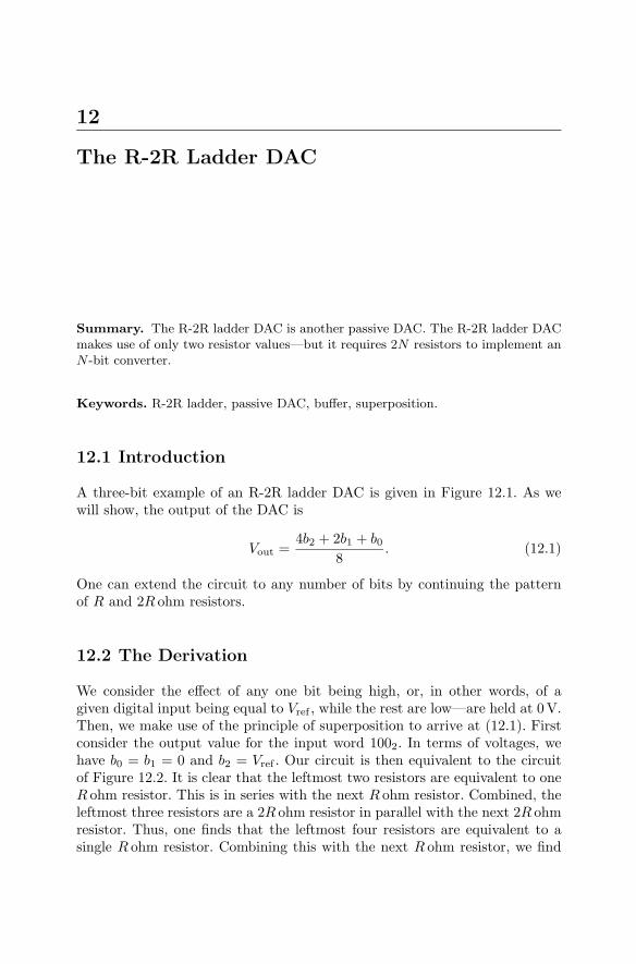
12
The R-2R Ladder DAC
Summary. The R-2R ladder DAC is another passive DAC. The R-2R ladder DACmakes use of only two resistor values—but it requires 2N resistors to implement anN -bit converter.
Keywords. R-2R ladder, passive DAC, buffer, superposition.
12.1 Introduction
A three-bit example of an R-2R ladder DAC is given in Figure 12.1. As wewill show, the output of the DAC is
Vout =4b2 + 2b1 + b0
8. (12.1)
One can extend the circuit to any number of bits by continuing the patternof R and 2R ohm resistors.
12.2 The Derivation
We consider the effect of any one bit being high, or, in other words, of agiven digital input being equal to Vref , while the rest are low—are held at 0 V.Then, we make use of the principle of superposition to arrive at (12.1). Firstconsider the output value for the input word 1002. In terms of voltages, wehave b0 = b1 = 0 and b2 = Vref . Our circuit is then equivalent to the circuitof Figure 12.2. It is clear that the leftmost two resistors are equivalent to oneR ohm resistor. This is in series with the next R ohm resistor. Combined, theleftmost three resistors are a 2R ohm resistor in parallel with the next 2R ohmresistor. Thus, one finds that the leftmost four resistors are equivalent to asingle R ohm resistor. Combining this with the next R ohm resistor, we find
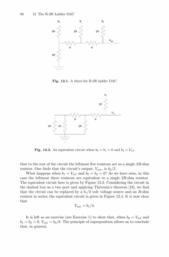
86 12 The R-2R Ladder DAC
Fig. 12.1. A three-bit R-2R ladder DAC
Fig. 12.2. An equivalent circuit when b0 = b1 = 0 and b2 = Vref
that to the rest of the circuit the leftmost five resistors act as a single 2R ohmresistor. One finds that the circuit’s output, Vout, is b2/2.
What happens when b1 = Vref and b0 = b2 = 0? As we have seen, in thiscase the leftmost three resistors are equivalent to a single 2R ohm resistor.The equivalent circuit here is given by Figure 12.3. Considering the circuit inthe dashed box as a two port and applying Thevenin’s theorem [18], we findthat the circuit can be replaced by a b1/2 volt voltage source and an R ohmresistor in series; the equivalent circuit is given in Figure 12.4. It is now clearthat
Vout = b1/4.
It is left as an exercise (see Exercise 1) to show that, when b0 = Vref andb1 = b2 = 0, Vout = b0/8. The principle of superposition allows us to concludethat, in general,
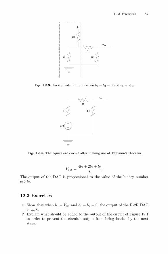
12.3 Exercises 87
Fig. 12.3. An equivalent circuit when b0 = b2 = 0 and b1 = Vref
Fig. 12.4. The equivalent circuit after making use of Thevinin’s theorem
Vout =4b2 + 2b1 + b0
8.
The output of the DAC is proportional to the value of the binary numberb2b1b0.
12.3 Exercises
1. Show that when b0 = Vref and b1 = b2 = 0, the output of the R-2R DACis b0/8.
2. Explain what should be added to the output of the circuit of Figure 12.1in order to prevent the circuit’s output from being loaded by the nextstage.
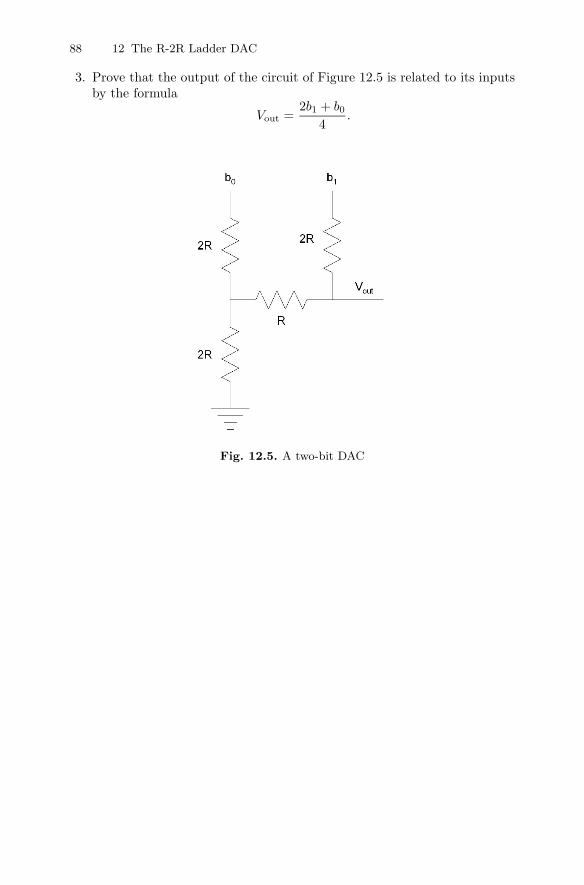
88 12 The R-2R Ladder DAC
3. Prove that the output of the circuit of Figure 12.5 is related to its inputsby the formula
Vout =2b1 + b0
4.
Fig. 12.5. A two-bit DAC
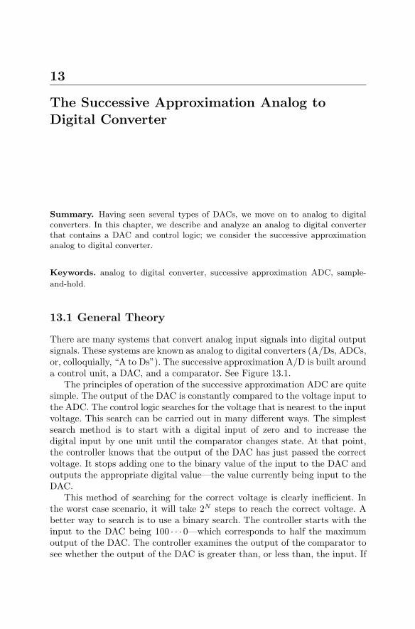
13
The Successive Approximation Analog toDigital Converter
Summary. Having seen several types of DACs, we move on to analog to digitalconverters. In this chapter, we describe and analyze an analog to digital converterthat contains a DAC and control logic; we consider the successive approximationanalog to digital converter.
Keywords. analog to digital converter, successive approximation ADC, sample-
and-hold.
13.1 General Theory
There are many systems that convert analog input signals into digital outputsignals. These systems are known as analog to digital converters (A/Ds, ADCs,or, colloquially, “A to Ds”). The successive approximation A/D is built arounda control unit, a DAC, and a comparator. See Figure 13.1.
The principles of operation of the successive approximation ADC are quitesimple. The output of the DAC is constantly compared to the voltage input tothe ADC. The control logic searches for the voltage that is nearest to the inputvoltage. This search can be carried out in many different ways. The simplestsearch method is to start with a digital input of zero and to increase thedigital input by one unit until the comparator changes state. At that point,the controller knows that the output of the DAC has just passed the correctvoltage. It stops adding one to the binary value of the input to the DAC andoutputs the appropriate digital value—the value currently being input to theDAC.
This method of searching for the correct voltage is clearly inefficient. Inthe worst case scenario, it will take 2N steps to reach the correct voltage. Abetter way to search is to use a binary search. The controller starts with theinput to the DAC being 100 · · · 0—which corresponds to half the maximumoutput of the DAC. The controller examines the output of the comparator tosee whether the output of the DAC is greater than, or less than, the input. If
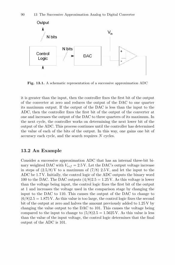
90 13 The Successive Approximation Analog to Digital Converter
Fig. 13.1. A schematic representation of a successive approximation ADC
it is greater than the input, then the controller fixes the first bit of the outputof the converter at zero and reduces the output of the DAC to one quarterits maximum output. If the output of the DAC is less than the input to theADC, then the controller fixes the first bit of the output of the converter atone and increases the output of the DAC to three quarters of its maximum. Inthe next cycle, the controller works on determining the next lower bit of theoutput of the ADC. This process continues until the controller has determinedthe value of each of the bits of the output. In this way, one gains one bit ofaccuracy each cycle, and the search requires N cycles.
13.2 An Example
Consider a successive approximation ADC that has an internal three-bit bi-nary weighted DAC with Vref = 2.5V. Let the DAC’s output voltage increasein steps of (2.5/8) V to a maximum of (7/8) 2.5 V, and let the input to theADC be 1.7 V. Initially, the control logic of the ADC outputs the binary word100 to the DAC. The DAC outputs (4/8)2.5 = 1.25V. As this voltage is lowerthan the voltage being input, the control logic fixes the first bit of the outputat 1 and increases the voltage used in the comparison stage by changing theinput to the DAC to 110. This causes the output of the DAC to change to(6/8)2.5 = 1.875V. As this value is too large, the control logic fixes the secondbit of the output at zero and halves the amount previously added to 1.25V bychanging the value output to the DAC to 101. This causes the voltage beingcompared to the input to change to (5/8)2.5 = 1.5625V. As this value is lessthan the value of the input voltage, the control logic determines that the finaloutput of the ADC is 101.
13.3 The Sample-and-hold Subsystem 91
13.3 The Sample-and-hold Subsystem
As described above, a successive approximation A/D compares the input volt-age to a reference voltage over a relatively long period of time. It is generallyimportant that the input to the A/D be forced to remain constant during theinterval in which the comparisons are being carried out. A schematic diagramof a subsystem that samples and holds an input value is given in Figure 13.2.Such subsystems are know as sample-and-hold circuits. When switch S1 isopen, the value on the capacitor should remain constant. When the switch isclosed, the voltage on the capacitor becomes equal to the voltage currently atthe input. By closing the switch briefly, one samples the input voltage, andby opening the switch one holds the previously sampled voltage. (This cir-cuit is a semi-practical implementation of the system whose properties werediscussed in Section 1.1.) When used with an A/D, the A/D must be forcednot to process the input until the output of the sample-and hold circuit hasconverged to the value of its input.
Fig. 13.2. A simple sample-and-hold circuit
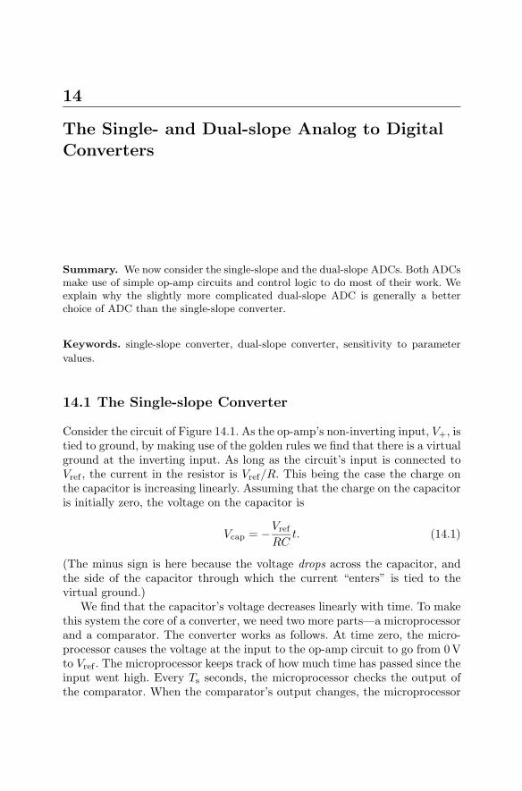
14
The Single- and Dual-slope Analog to DigitalConverters
Summary. We now consider the single-slope and the dual-slope ADCs. Both ADCsmake use of simple op-amp circuits and control logic to do most of their work. Weexplain why the slightly more complicated dual-slope ADC is generally a betterchoice of ADC than the single-slope converter.
Keywords. single-slope converter, dual-slope converter, sensitivity to parameter
values.
14.1 The Single-slope Converter
Consider the circuit of Figure 14.1. As the op-amp’s non-inverting input, V+, istied to ground, by making use of the golden rules we find that there is a virtualground at the inverting input. As long as the circuit’s input is connected toVref , the current in the resistor is Vref/R. This being the case the charge onthe capacitor is increasing linearly. Assuming that the charge on the capacitoris initially zero, the voltage on the capacitor is
Vcap = −Vref
RCt. (14.1)
(The minus sign is here because the voltage drops across the capacitor, andthe side of the capacitor through which the current “enters” is tied to thevirtual ground.)
We find that the capacitor’s voltage decreases linearly with time. To makethis system the core of a converter, we need two more parts—a microprocessorand a comparator. The converter works as follows. At time zero, the micro-processor causes the voltage at the input to the op-amp circuit to go from 0Vto Vref . The microprocessor keeps track of how much time has passed since theinput went high. Every Ts seconds, the microprocessor checks the output ofthe comparator. When the comparator’s output changes, the microprocessor
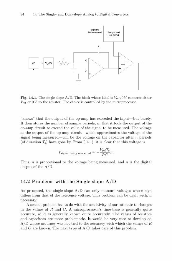
94 14 The Single- and Dual-slope Analog to Digital Converters
Fig. 14.1. The single-slope A/D. The block whose label is Vref/0 V connects eitherVref or 0 V to the resistor. The choice is controlled by the microprocessor.
“knows” that the output of the op-amp has exceeded the input—but barely.It then stores the number of sample periods, n, that it took the output of theop-amp circuit to exceed the value of the signal to be measured. The voltageat the output of the op-amp circuit—which approximates the voltage of thesignal being measured—will be the voltage on the capacitor after n periods(of duration Ts) have gone by. From (14.1), it is clear that this voltage is
Vsignal being measured ≈ −VrefTs
RCn.
Thus, n is proportional to the voltage being measured, and n is the digitaloutput of the A/D.
14.2 Problems with the Single-slope A/D
As presented, the single-slope A/D can only measure voltages whose signdiffers from that of the reference voltage. This problem can be dealt with, ifnecessary.
A second problem has to do with the sensitivity of our estimate to changesin the values of R and C. A microprocessor’s time-base is generally quiteaccurate, so Ts is generally known quite accurately. The values of resistorsand capacitors are more problematic. It would be very nice to develop anA/D whose accuracy was not tied to the accuracy with which the values of Rand C are known. The next type of A/D takes care of this problem.
14.4 A Simple Example 95
14.3 The Dual-slope A/D
Consider the circuit of Figure 14.2. The circuit is very similar to the single-slope A/D. There are two major differences
• the input to the op-amp circuit can be either Vref or the signal to bemeasured, and
• the comparator checks when the output of the op-amp circuit returns tozero.
In this circuit, the microprocessor initially sets the input to the op-ampcircuit to the voltage to be measured for n clock cycles. It then switches theinput to the op-amp circuit to Vref—which must be opposite in polarity tothe voltage to be measured. It maintains this voltage until the cycle in whichthe comparator determines that the sign of the output of the op-amp circuithas changed. Suppose that this take m cycles from the point at which themicroprocessor switches the voltage source. Following the logic used in thecase of the single-slope converter, we find that
Vin
RCTsn +
Vref
RCTsm ≈ 0.
Solving for Vin, we find that
Vin ≈ −Vref
nm.
We find that Vin is proportional to m. Thus, m is the digital version of thevoltage Vin. The beauty of this system is that the constant of proportionalityis no longer a function of R or C. We can now use less expensive resistors andcapacitors in our design, and we no longer need to worry (much) about theeffects of aging or temperature on the values of R or C.
14.4 A Simple Example
Let Ts = 100μ s, n = 10, and let Vref = −2.5V. Suppose that R = 100Kand C = 10nF, and let Vin = 1.1V. Assuming that at time t = 0—whenthe measurement begins—the capacitor is fully discharged, during the firstmillisecond the voltage at the output of the op-amp will be
VC =−Vin
RCt = −1,100t.
From this point on, the output will be
VC =−Vref
RC(t − 0.001) − 1.1 = 2,500(t − 0.001) − 1.1.
96 14 The Single- and Dual-slope Analog to Digital Converters
Fig. 14.2. The dual-slope A/D
(See Figure 14.3 to see the output of the “op-amp” of a Simulink model of thisA/D.) It is easy to see that VC goes from negative to positive when t = 1.44 ms.Thus, the final value of m will be 5. This corresponds to an estimate of
Vin ≈ 2.510
5 = 1.25V.
14.5 Exercises
1. Repeat the calculations of Section 14.4, but let n = 20. What is theestimated value of Vin at the end of the conversion?
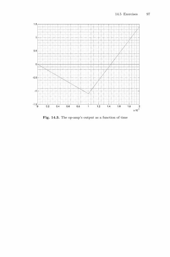
14.5 Exercises 97
Fig. 14.3. The op-amp’s output as a function of time
15
The Pipelined A/D
Summary. We now consider the pipelined A/D. This A/D is constructed by“stringing together” several identical subunits. The pipelined A/D generally hasa high throughput—it processes a lot of analog data quickly. The pipelined A/Dsuffers from processing delay, however.
Keywords. pipelined A/D, latency, accuracy, processing delay.
15.1 Introduction
If one would like an A/D that is capable of reasonably high accuracy, isreasonably fast, and is not too expensive, a pipelined A/D may be a goodchoice. A pipelined A/D is composed of many identical units like the unitshown in Figure 15.1.
The first stage in the unit is a sample-and-hold circuit. The next stageis an analog to digital converter. The output bit(s) of this converter becomesome of the bits in the final output of the converter. Next, a D/A reconvertsthe digital word to an analog voltage. (The levels of the A/D and the D/A aredesigned to be identical.) The next stage is to calculate the difference of theoutput of the D/A and the input voltage. The difference of the voltages is the“unconverted” part of the input voltage. The last stage rescales the output ofthe differencer so that its range is, once again, the full range of the A/D. Thisvoltage contains the “unconverted” part of the signal, and by processing therescaled “remainder” it is possible to make the conversion more accurate.
The idea that underlies the pipelined converter is that by cascading severalblocks like that of Figure 15.1, one can make an arbitrarily precise A/D. Eachblock takes its input, converts several bits, and outputs a voltage that isproportional to the portion of its input that the block did not convert. Thenext block “sees” the output of the previous block—which is proportional tothe unconverted part of the input—and extracts a few more bits from it. Thisprocess continues down the pipeline.
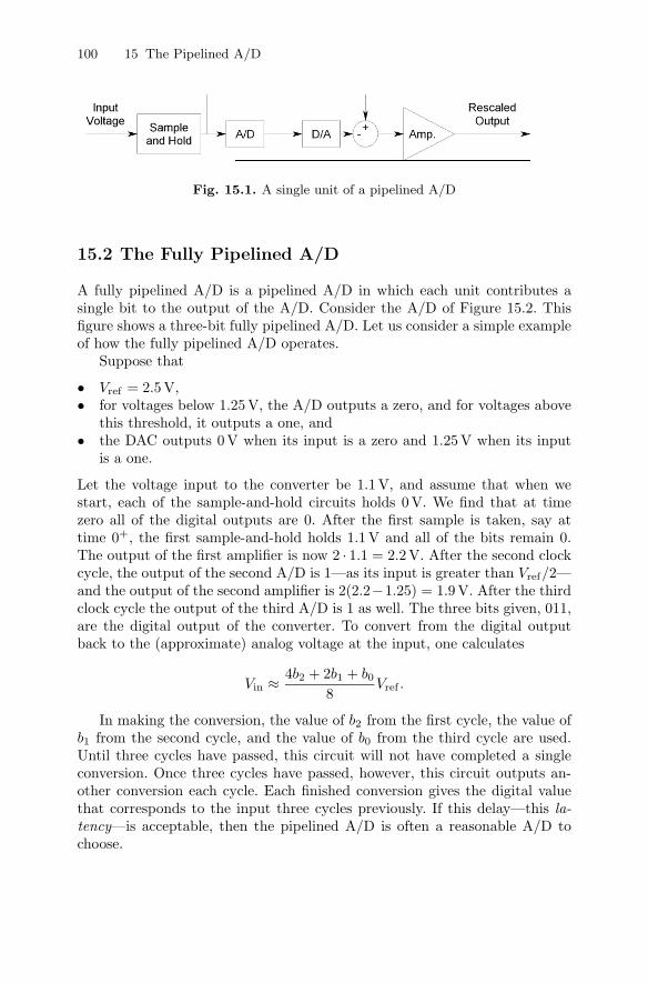
100 15 The Pipelined A/D
Fig. 15.1. A single unit of a pipelined A/D
15.2 The Fully Pipelined A/D
A fully pipelined A/D is a pipelined A/D in which each unit contributes asingle bit to the output of the A/D. Consider the A/D of Figure 15.2. Thisfigure shows a three-bit fully pipelined A/D. Let us consider a simple exampleof how the fully pipelined A/D operates.
Suppose that
• Vref = 2.5V,• for voltages below 1.25 V, the A/D outputs a zero, and for voltages above
this threshold, it outputs a one, and• the DAC outputs 0 V when its input is a zero and 1.25 V when its input
is a one.
Let the voltage input to the converter be 1.1 V, and assume that when westart, each of the sample-and-hold circuits holds 0 V. We find that at timezero all of the digital outputs are 0. After the first sample is taken, say attime 0+, the first sample-and-hold holds 1.1 V and all of the bits remain 0.The output of the first amplifier is now 2 · 1.1 = 2.2V. After the second clockcycle, the output of the second A/D is 1—as its input is greater than Vref/2—and the output of the second amplifier is 2(2.2−1.25) = 1.9V. After the thirdclock cycle the output of the third A/D is 1 as well. The three bits given, 011,are the digital output of the converter. To convert from the digital outputback to the (approximate) analog voltage at the input, one calculates
Vin ≈ 4b2 + 2b1 + b0
8Vref .
In making the conversion, the value of b2 from the first cycle, the value ofb1 from the second cycle, and the value of b0 from the third cycle are used.Until three cycles have passed, this circuit will not have completed a singleconversion. Once three cycles have passed, however, this circuit outputs an-other conversion each cycle. Each finished conversion gives the digital valuethat corresponds to the input three cycles previously. If this delay—this la-tency—is acceptable, then the pipelined A/D is often a reasonable A/D tochoose.
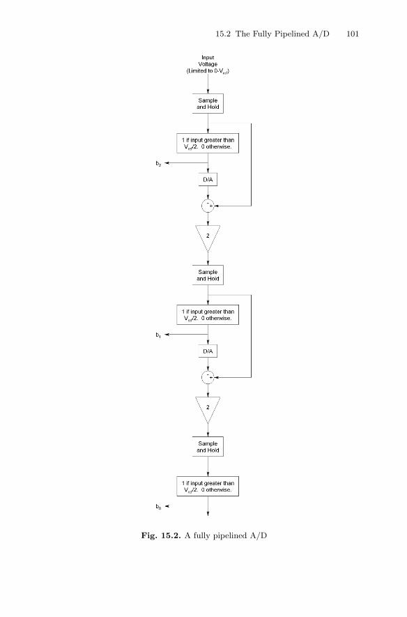
15.2 The Fully Pipelined A/D 101
Fig. 15.2. A fully pipelined A/D

102 15 The Pipelined A/D
15.3 The Experiment
Using Simulink r©, build a three-stage pipelined A/D converter. You may needto use two sample-and-hold blocks (one that samples on the rising edge andone on the falling edge) for each sample-and-hold circuit.
Connect the digital outputs of the A/D to a new block—a D/A—that willconvert the digital signals back into analog signals. (Note that there will besynchronization issues to deal with here as well.)
15.4 Exercises
1. Let the values of the input to the circuit of Figure 15.2 be {1.0, 1.5, 2.3, 2.4}at the first four cycles of the A/D’s operation. Let Vref = 2.5V, and assumethat all the sample-and-holds initially hold 0 V. Find the values of b2, b1,and b0 and the values of the outputs of the amplifiers for the first fourperiods of the A/D’s operation. Explain how to take the calculated valuesand produce the digital outputs that correspond to the first and secondanalog inputs.
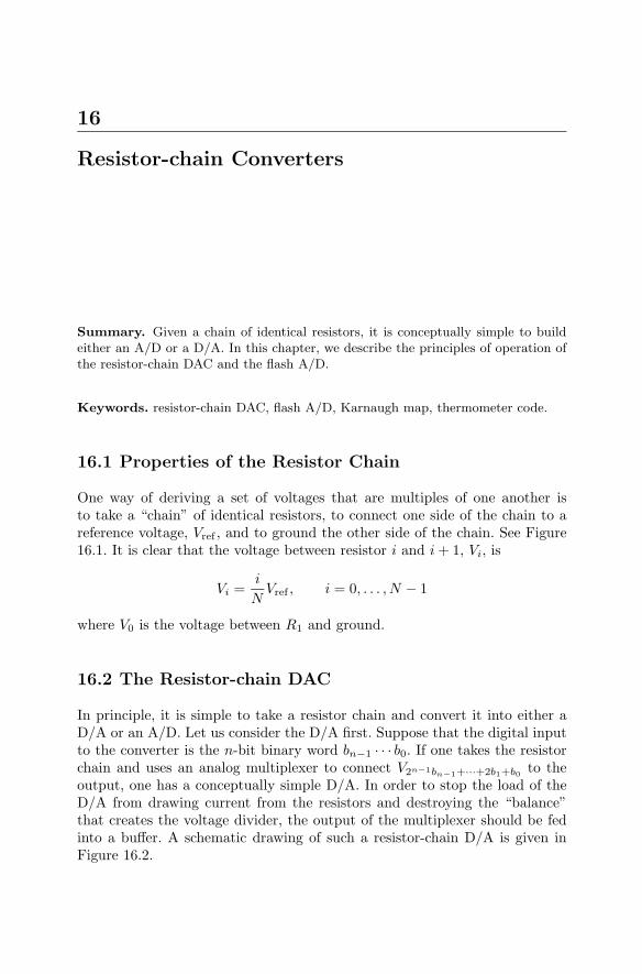
16
Resistor-chain Converters
Summary. Given a chain of identical resistors, it is conceptually simple to buildeither an A/D or a D/A. In this chapter, we describe the principles of operation ofthe resistor-chain DAC and the flash A/D.
Keywords. resistor-chain DAC, flash A/D, Karnaugh map, thermometer code.
16.1 Properties of the Resistor Chain
One way of deriving a set of voltages that are multiples of one another isto take a “chain” of identical resistors, to connect one side of the chain to areference voltage, Vref , and to ground the other side of the chain. See Figure16.1. It is clear that the voltage between resistor i and i + 1, Vi, is
Vi =i
NVref , i = 0, . . . , N − 1
where V0 is the voltage between R1 and ground.
16.2 The Resistor-chain DAC
In principle, it is simple to take a resistor chain and convert it into either aD/A or an A/D. Let us consider the D/A first. Suppose that the digital inputto the converter is the n-bit binary word bn−1 · · · b0. If one takes the resistorchain and uses an analog multiplexer to connect V2n−1bn−1+···+2b1+b0 to theoutput, one has a conceptually simple D/A. In order to stop the load of theD/A from drawing current from the resistors and destroying the “balance”that creates the voltage divider, the output of the multiplexer should be fedinto a buffer. A schematic drawing of such a resistor-chain D/A is given inFigure 16.2.
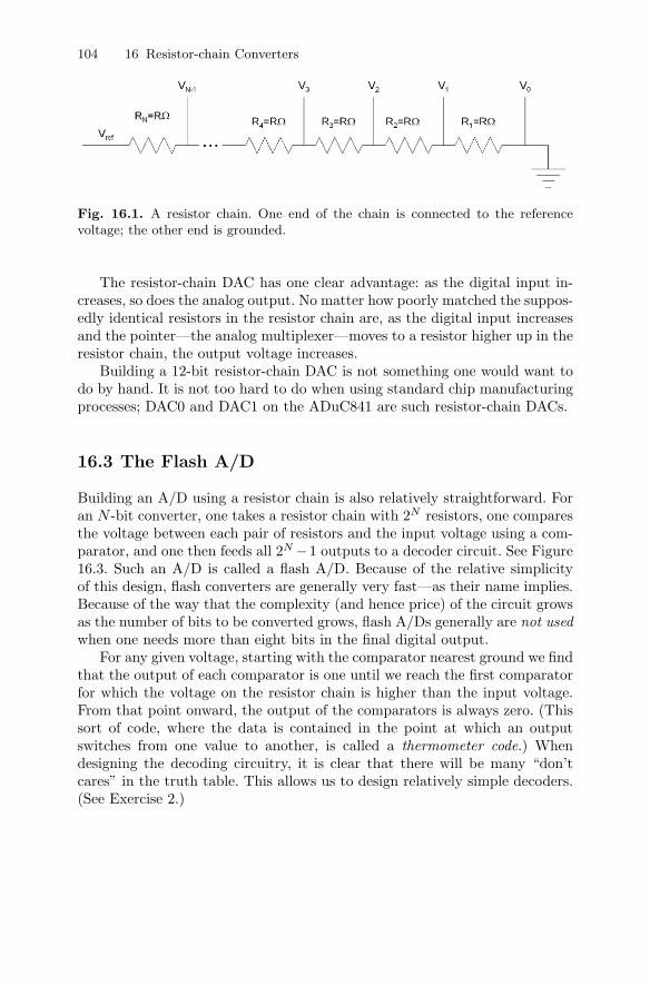
104 16 Resistor-chain Converters
Fig. 16.1. A resistor chain. One end of the chain is connected to the referencevoltage; the other end is grounded.
The resistor-chain DAC has one clear advantage: as the digital input in-creases, so does the analog output. No matter how poorly matched the suppos-edly identical resistors in the resistor chain are, as the digital input increasesand the pointer—the analog multiplexer—moves to a resistor higher up in theresistor chain, the output voltage increases.
Building a 12-bit resistor-chain DAC is not something one would want todo by hand. It is not too hard to do when using standard chip manufacturingprocesses; DAC0 and DAC1 on the ADuC841 are such resistor-chain DACs.
16.3 The Flash A/D
Building an A/D using a resistor chain is also relatively straightforward. Foran N -bit converter, one takes a resistor chain with 2N resistors, one comparesthe voltage between each pair of resistors and the input voltage using a com-parator, and one then feeds all 2N −1 outputs to a decoder circuit. See Figure16.3. Such an A/D is called a flash A/D. Because of the relative simplicityof this design, flash converters are generally very fast—as their name implies.Because of the way that the complexity (and hence price) of the circuit growsas the number of bits to be converted grows, flash A/Ds generally are not usedwhen one needs more than eight bits in the final digital output.
For any given voltage, starting with the comparator nearest ground we findthat the output of each comparator is one until we reach the first comparatorfor which the voltage on the resistor chain is higher than the input voltage.From that point onward, the output of the comparators is always zero. (Thissort of code, where the data is contained in the point at which an outputswitches from one value to another, is called a thermometer code.) Whendesigning the decoding circuitry, it is clear that there will be many “don’tcares” in the truth table. This allows us to design relatively simple decoders.(See Exercise 2.)
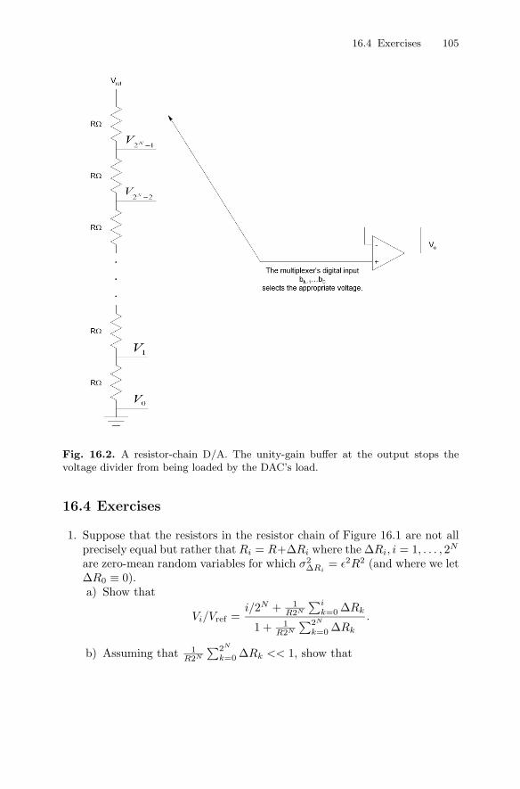
16.4 Exercises 105
Fig. 16.2. A resistor-chain D/A. The unity-gain buffer at the output stops thevoltage divider from being loaded by the DAC’s load.
16.4 Exercises
1. Suppose that the resistors in the resistor chain of Figure 16.1 are not allprecisely equal but rather that Ri = R+ΔRi where the ΔRi, i = 1, . . . , 2N
are zero-mean random variables for which σ2ΔRi
= ε2R2 (and where we letΔR0 ≡ 0).a) Show that
Vi/Vref =i/2N + 1
R2N
∑ik=0 ΔRk
1 + 1R2N
∑2N
k=0 ΔRk
.
b) Assuming that 1R2N
∑2N
k=0 ΔRk << 1, show that
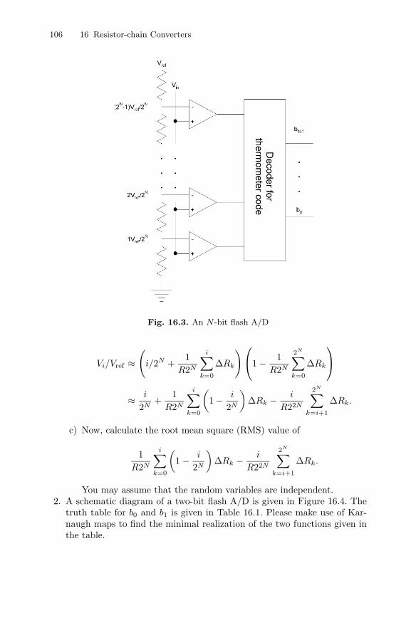
106 16 Resistor-chain Converters
Fig. 16.3. An N -bit flash A/D
Vi/Vref ≈(
i/2N +1
R2N
i∑
k=0
ΔRk
)⎛
⎝1 − 1R2N
2N∑
k=0
ΔRk
⎞
⎠
≈ i
2N+
1R2N
i∑
k=0
(1 − i
2N
)ΔRk − i
R22N
2N∑
k=i+1
ΔRk.
c) Now, calculate the root mean square (RMS) value of
1R2N
i∑
k=0
(1 − i
2N
)ΔRk − i
R22N
2N∑
k=i+1
ΔRk.
You may assume that the random variables are independent.2. A schematic diagram of a two-bit flash A/D is given in Figure 16.4. The
truth table for b0 and b1 is given in Table 16.1. Please make use of Kar-naugh maps to find the minimal realization of the two functions given inthe table.
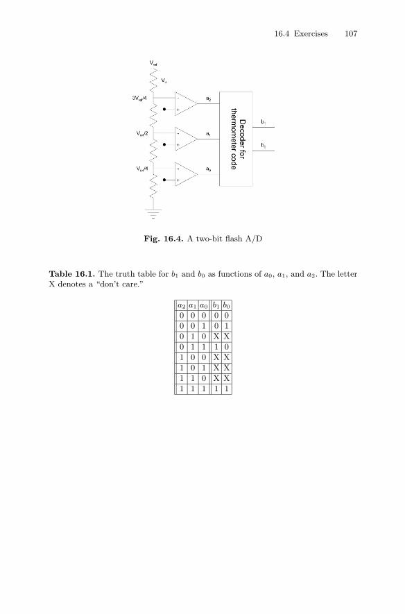
16.4 Exercises 107
Fig. 16.4. A two-bit flash A/D
Table 16.1. The truth table for b1 and b0 as functions of a0, a1, and a2. The letterX denotes a “don’t care.”
a2 a1 a0 b1 b0
0 0 0 0 0
0 0 1 0 1
0 1 0 X X
0 1 1 1 0
1 0 0 X X
1 0 1 X X
1 1 0 X X
1 1 1 1 1
17
Sigma–Delta Converters
Summary. By making use of feedback in an interesting way, it is possible to designvery accurate ADCs and DACs. In this chapter, we consider the sigma–delta A/Dand the sigma–delta D/A. We find that though they can be very accurate, whenthey are most accurate they are also very slow.
Keywords. sigma–delta DAC, sigma–delta A/D, feedback, noise shaping, oversam-
pling.
17.1 Introduction
We now consider sigma–delta (Σ–Δ) converters. Such converters make use ofsums (from whence the Σ), differences (from whence the Δ), feedback, andlow-pass filters in order to do their jobs. A generic sigma–delta converter isshown in Figure 17.1. This system can be considered a simplified model of anA/D or a D/A. Upon considering Vin(s), N(s), and Y (s), we find that
Y (s) = N(s) +K
s(Vin(s) − Y (s)).
Solving for the output of the feedback system, Y (s), we find that
Y (s) =s
K + sN(s) +
K
K + sVin(s). (17.1)
What is critical here is that for small values of s = jω—for low frequencies—the noise term, N(s), is attenuated greatly while the input is passed along al-most without change. (Sigma–delta modulators are said to “shape” the noisespectrum and to have a noise-shaping property.) The low-pass filter throughwhich Y (s) passes should remove the noise component—which is largely lo-cated at high frequencies—without affecting the input, which is assumed tohave a low-pass character.
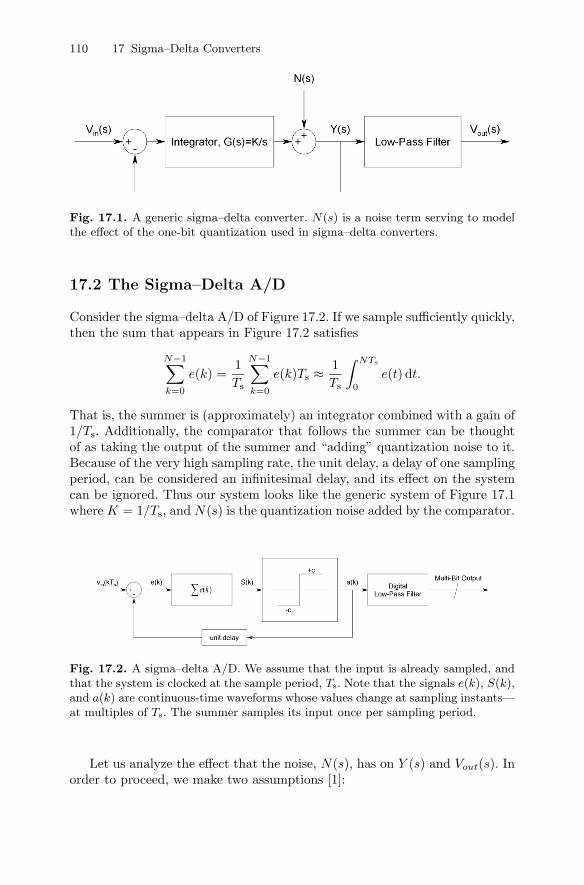
110 17 Sigma–Delta Converters
Fig. 17.1. A generic sigma–delta converter. N(s) is a noise term serving to modelthe effect of the one-bit quantization used in sigma–delta converters.
17.2 The Sigma–Delta A/D
Consider the sigma–delta A/D of Figure 17.2. If we sample sufficiently quickly,then the sum that appears in Figure 17.2 satisfies
N−1∑
k=0
e(k) =1Ts
N−1∑
k=0
e(k)Ts ≈ 1Ts
∫ NTs
0
e(t) dt.
That is, the summer is (approximately) an integrator combined with a gain of1/Ts. Additionally, the comparator that follows the summer can be thoughtof as taking the output of the summer and “adding” quantization noise to it.Because of the very high sampling rate, the unit delay, a delay of one samplingperiod, can be considered an infinitesimal delay, and its effect on the systemcan be ignored. Thus our system looks like the generic system of Figure 17.1where K = 1/Ts, and N(s) is the quantization noise added by the comparator.
Fig. 17.2. A sigma–delta A/D. We assume that the input is already sampled, andthat the system is clocked at the sample period, Ts. Note that the signals e(k), S(k),and a(k) are continuous-time waveforms whose values change at sampling instants—at multiples of Ts. The summer samples its input once per sampling period.
Let us analyze the effect that the noise, N(s), has on Y (s) and Vout(s). Inorder to proceed, we make two assumptions [1]:
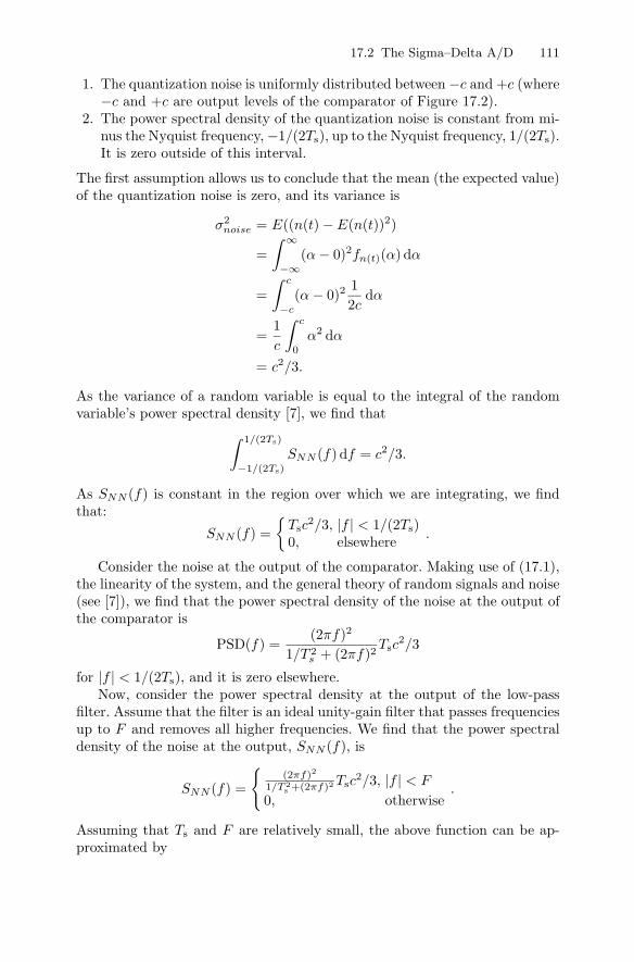
17.2 The Sigma–Delta A/D 111
1. The quantization noise is uniformly distributed between −c and +c (where−c and +c are output levels of the comparator of Figure 17.2).
2. The power spectral density of the quantization noise is constant from mi-nus the Nyquist frequency, −1/(2Ts), up to the Nyquist frequency, 1/(2Ts).It is zero outside of this interval.
The first assumption allows us to conclude that the mean (the expected value)of the quantization noise is zero, and its variance is
σ2noise = E((n(t) − E(n(t))2)
=∫ ∞
−∞(α − 0)2fn(t)(α) dα
=∫ c
−c
(α − 0)212c
dα
=1c
∫ c
0
α2 dα
= c2/3.
As the variance of a random variable is equal to the integral of the randomvariable’s power spectral density [7], we find that
∫ 1/(2Ts)
−1/(2Ts)
SNN (f) df = c2/3.
As SNN (f) is constant in the region over which we are integrating, we findthat:
SNN (f) ={
Tsc2/3, |f | < 1/(2Ts)
0, elsewhere .
Consider the noise at the output of the comparator. Making use of (17.1),the linearity of the system, and the general theory of random signals and noise(see [7]), we find that the power spectral density of the noise at the output ofthe comparator is
PSD(f) =(2πf)2
1/T 2s + (2πf)2
Tsc2/3
for |f | < 1/(2Ts), and it is zero elsewhere.Now, consider the power spectral density at the output of the low-pass
filter. Assume that the filter is an ideal unity-gain filter that passes frequenciesup to F and removes all higher frequencies. We find that the power spectraldensity of the noise at the output, SNN (f), is
SNN (f) =
{(2πf)2
1/T 2s +(2πf)2 Tsc
2/3, |f | < F
0, otherwise.
Assuming that Ts and F are relatively small, the above function can be ap-proximated by
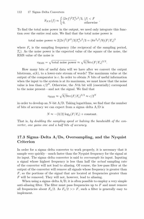
112 17 Sigma–Delta Converters
SNN (f) ≈{
(2πf)2T 3s c2/3, |f | < F
0, otherwise .
To find the total noise power in the output, we need only integrate this func-tion over the entire real axis. We find that the total noise power is
total noise power ≈ 2(2π)2(F 3/3)T 3s c2/3 = (8π2c2/9)(F/Fs)3
where Fs is the sampling frequency (the reciprocal of the sampling period,Ts). As the noise power is the expected value of the square of the noise, theRMS value of the noise is
vRMS =√
total noise power ≈√
8/9πc(F/Fs)3/2.
How many bits of useful data will we have after we convert the outputbitstream, a(k), to a lower-rate stream of words? The maximum value at theoutput of the comparator is c. In order to obtain N bits of useful informationwhen the input to the system is at its maximum, we must know that the noisevalue is less than c/2N . Otherwise, the Nth bit will (essentially) correspondto the noise present—and not the signal. We find that
vRMS ≈√
8/9πc(F/Fs)3/2 ≈ c/2N
in order to develop an N -bit A/D. Taking logarithms, we find that the numberof bits of accuracy we can expect from a sigma–delta A/D is
N ≈ −(3/2) log2(F/Fs) + constant.
That is, by doubling the sampling speed or halving the bandwidth of the con-verter, one gains one and a half bits of accuracy.
17.3 Sigma–Delta A/Ds, Oversampling, and the NyquistCriterion
In order for a sigma–delta converter to work properly, it is necessary that itsample very quickly—much faster than the Nyquist frequency for the signal atits input. The sigma–delta converter is said to oversample its input. Inputinga signal whose highest frequency is less than half the actual sampling rateof the converter will not lead to aliasing. Of course, the low-pass filter at theoutput of the converter will remove all signals whose frequency is greater thanF , so the portions of the signal that are located at frequencies greater thanF will be removed. They will not, however, lead to aliasing.
When using a sigma–delta A/D, it is often possible to employ a very simpleanti-aliasing filter. The filter must pass frequencies up to F and must removeall frequencies about Fs/2. As Fs/2 >> F , such a filter is generally easy toimplement.
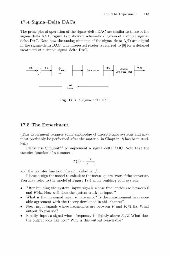
17.5 The Experiment 113
17.4 Sigma–Delta DACs
The principles of operation of the sigma–delta DAC are similar to those of thesigma–delta A/D. Figure 17.3 shows a schematic diagram of a simple sigma–delta DAC. Note how the analog elements of the sigma–delta A/D are digitalin the sigma–delta DAC. The interested reader is referred to [8] for a detailedtreatment of a simple sigma–delta DAC.
Fig. 17.3. A sigma–delta DAC
17.5 The Experiment
(This experiment requires some knowledge of discrete-time systems and maymost profitably be performed after the material in Chapter 18 has been stud-ied.)
Please use Simulink r© to implement a sigma–delta ADC. Note that thetransfer function of a summer is
T (z) =z
z − 1,
and the transfer function of a unit delay is 1/z.Please design the model to calculate the mean square error of the converter.
You may refer to the model of Figure 17.4 while building your system.
• After building the system, input signals whose frequencies are between 0and F Hz. How well does the system track its inputs?
• What is the measured mean square error? Is the measurement in reason-able agreement with the theory developed in this chapter?
• Now, input signals whose frequencies are between F and Fs/2 Hz. Whatoutput do you see?
• Finally, input a signal whose frequency is slightly above Fs/2. What doesthe output look like now? Why is this output reasonable?
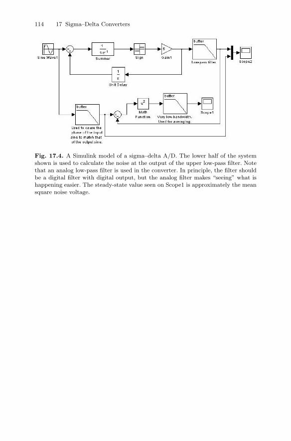
114 17 Sigma–Delta Converters
Fig. 17.4. A Simulink model of a sigma–delta A/D. The lower half of the systemshown is used to calculate the noise at the output of the upper low-pass filter. Notethat an analog low-pass filter is used in the converter. In principle, the filter shouldbe a digital filter with digital output, but the analog filter makes “seeing” what ishappening easier. The steady-state value seen on Scope1 is approximately the meansquare noise voltage.

Part III
Digital Filters
18
Discrete-time Systems and the Z-transform
Summary. In engineering, most subject areas make use of specific mathematicaltools. In the design and analysis of discrete-time systems, the most important of themathematical tools is the Z-transform. In this chapter, we develop the Z-transformand its properties, and we show how to make use of the Z-transform to analyzediscrete-time linear time-invariant systems. In the following chapters, we treat theproblem of digital filter design.
Keywords. Z-transform, LTI system, region of convergence, sinusoidal steady state,
stability.
18.1 The Definition of the Z-transform
Given a doubly infinite sequence of values {. . . , a−1, a0, a1, . . .}, we define thetwo-sided (or bilateral) Z-transform of the sequence, A(z), by the equation
A(z) ≡∞∑
k=−∞akz−k. (18.1)
We generally use lowercase letters to represent sequences and uppercase lettersto represent Z-transforms. As we see shortly, the Z-transform has many niceproperties.
18.2 Properties of the Z-transform
18.2.1 The Region of Convergence (ROC)
The Z-transform of the sequence {ak} can be written
A(z) =∞∑
k=−∞akz−k =
−1∑
k=−∞akz−k +
∞∑
k=0
akz−k.
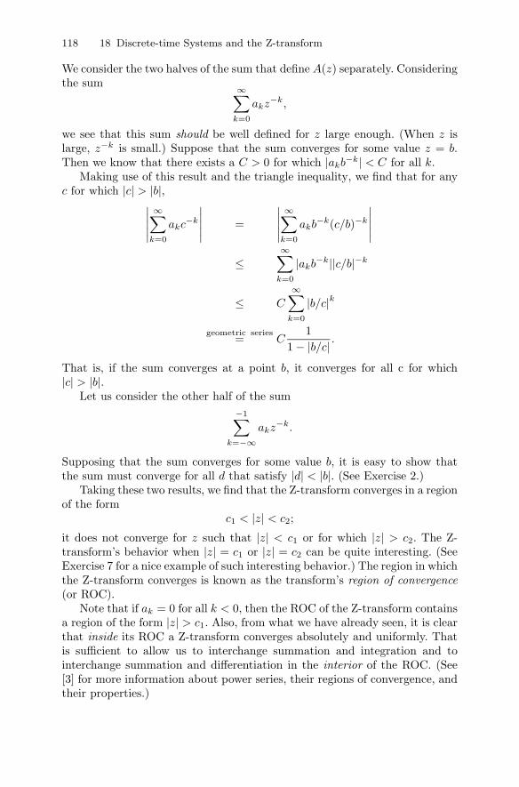
118 18 Discrete-time Systems and the Z-transform
We consider the two halves of the sum that define A(z) separately. Consideringthe sum ∞∑
k=0
akz−k,
we see that this sum should be well defined for z large enough. (When z islarge, z−k is small.) Suppose that the sum converges for some value z = b.Then we know that there exists a C > 0 for which |akb−k| < C for all k.
Making use of this result and the triangle inequality, we find that for anyc for which |c| > |b|,
∣∣∣∣∣
∞∑
k=0
akc−k
∣∣∣∣∣ =
∣∣∣∣∣
∞∑
k=0
akb−k(c/b)−k
∣∣∣∣∣
≤∞∑
k=0
|akb−k||c/b|−k
≤ C
∞∑
k=0
|b/c|k
geometric series= C
11 − |b/c| .
That is, if the sum converges at a point b, it converges for all c for which|c| > |b|.
Let us consider the other half of the sum−1∑
k=−∞akz−k.
Supposing that the sum converges for some value b, it is easy to show thatthe sum must converge for all d that satisfy |d| < |b|. (See Exercise 2.)
Taking these two results, we find that the Z-transform converges in a regionof the form
c1 < |z| < c2;
it does not converge for z such that |z| < c1 or for which |z| > c2. The Z-transform’s behavior when |z| = c1 or |z| = c2 can be quite interesting. (SeeExercise 7 for a nice example of such interesting behavior.) The region in whichthe Z-transform converges is known as the transform’s region of convergence(or ROC).
Note that if ak = 0 for all k < 0, then the ROC of the Z-transform containsa region of the form |z| > c1. Also, from what we have already seen, it is clearthat inside its ROC a Z-transform converges absolutely and uniformly. Thatis sufficient to allow us to interchange summation and integration and tointerchange summation and differentiation in the interior of the ROC. (See[3] for more information about power series, their regions of convergence, andtheir properties.)
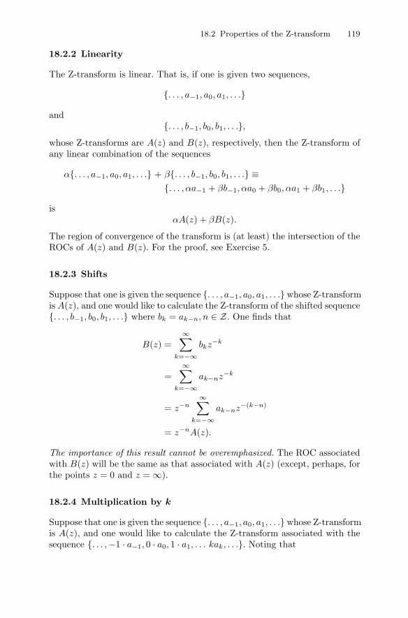
18.2 Properties of the Z-transform 119
18.2.2 Linearity
The Z-transform is linear. That is, if one is given two sequences,
{. . . , a−1, a0, a1, . . .}
and{. . . , b−1, b0, b1, . . .},
whose Z-transforms are A(z) and B(z), respectively, then the Z-transform ofany linear combination of the sequences
α{. . . , a−1, a0, a1, . . .} + β{. . . , b−1, b0, b1, . . .} ≡{. . . , αa−1 + βb−1, αa0 + βb0, αa1 + βb1, . . .}
isαA(z) + βB(z).
The region of convergence of the transform is (at least) the intersection of theROCs of A(z) and B(z). For the proof, see Exercise 5.
18.2.3 Shifts
Suppose that one is given the sequence {. . . , a−1, a0, a1, . . .} whose Z-transformis A(z), and one would like to calculate the Z-transform of the shifted sequence{. . . , b−1, b0, b1, . . .} where bk = ak−n, n ∈ Z. One finds that
B(z) =∞∑
k=−∞bkz−k
=∞∑
k=−∞ak−nz−k
= z−n∞∑
k=−∞ak−nz−(k−n)
= z−nA(z).
The importance of this result cannot be overemphasized. The ROC associatedwith B(z) will be the same as that associated with A(z) (except, perhaps, forthe points z = 0 and z = ∞).
18.2.4 Multiplication by k
Suppose that one is given the sequence {. . . , a−1, a0, a1, . . .} whose Z-transformis A(z), and one would like to calculate the Z-transform associated with thesequence {. . . ,−1 · a−1, 0 · a0, 1 · a1, . . . kak, . . .}. Noting that
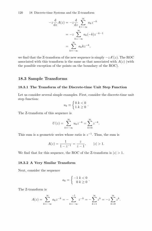
120 18 Discrete-time Systems and the Z-transform
−zddz
A(z) = −zddz
∞∑
k=−∞akz−k
= −z
∞∑
k=−∞ak(−k)z−k−1
=∞∑
k=−∞akkz−k,
we find that the Z-transform of the new sequence is simply −zA′(z). The ROCassociated with this transform is the same as that associated with A(z) (withthe possible exception of the points on the boundary of the ROC).
18.3 Sample Transforms
18.3.1 The Transform of the Discrete-time Unit Step Function
Let us consider several simple examples. First, consider the discrete-time unitstep function:
uk ≡{
0 k < 01 k ≥ 0 .
The Z-transform of this sequence is
U(z) =∞∑
k=−∞ukz−k =
∞∑
k=0
z−k.
This sum is a geometric series whose ratio is z−1. Thus, the sum is
A(z) =1
1 − z−1=
z
z − 1, |z| > 1.
We find that for this sequence, the ROC of the Z-transform is |z| > 1.
18.3.2 A Very Similar Transform
Next, consider the sequence
ak ={−1 k < 0
0 k ≥ 0 .
The Z-transform is
A(z) =∞∑
k=−∞akz−k = −
−1∑
k=−∞z−k = −
∞∑
k=1
zk = −z
∞∑
k=0
zk.
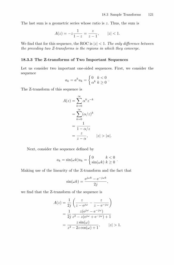
18.3 Sample Transforms 121
The last sum is a geometric series whose ratio is z. Thus, the sum is
A(z) = −z1
1 − z=
z
z − 1, |z| < 1.
We find that for this sequence, the ROC is |z| < 1. The only difference betweenthe preceding two Z-transforms is the regions in which they converge.
18.3.3 The Z-transforms of Two Important Sequences
Let us consider two important one-sided sequences. First, we consider thesequence
ak = akuk ={
0 k < 0αk k ≥ 0 .
The Z-transform of this sequence is
A(z) =∞∑
k=0
αkz−k
=∞∑
k=0
(α/z)k
=1
1 − α/z
=z
z − α, |z| > |α|.
Next, consider the sequence defined by
ak = sin(ωk)uk ={
0 k < 0sin(ωk) k ≥ 0 .
Making use of the linearity of the Z-transform and the fact that
sin(ωk) =ejωk − e−jωk
2j,
we find that the Z-transform of the sequence is
A(z) =12j
(z
z − ejω− z
z − e−jω
)
=12j
z(ejω − e−jω)z2 − z(ejω + e−jω) + 1
=z sin(ω)
z2 − 2z cos(ω) + 1, |z| > 1.
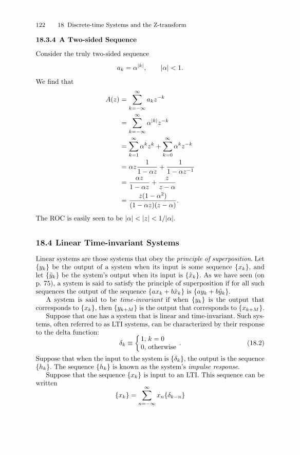
122 18 Discrete-time Systems and the Z-transform
18.3.4 A Two-sided Sequence
Consider the truly two-sided sequence
ak = α|k|, |α| < 1.
We find that
A(z) =∞∑
k=−∞akz−k
=∞∑
k=−∞α|k|z−k
=∞∑
k=1
αkzk +∞∑
k=0
αkz−k
= αz1
1 − αz+
11 − αz−1
=αz
1 − αz+
z
z − α
=z(1 − α2)
(1 − αz)(z − α).
The ROC is easily seen to be |α| < |z| < 1/|α|.
18.4 Linear Time-invariant Systems
Linear systems are those systems that obey the principle of superposition. Let{yk} be the output of a system when its input is some sequence {xk}, andlet {yk} be the system’s output when its input is {xk}. As we have seen (onp. 75), a system is said to satisfy the principle of superposition if for all suchsequences the output of the sequence {axk + bxk} is {ayk + byk}.
A system is said to be time-invariant if when {yk} is the output thatcorresponds to {xk}, then {yk+M} is the output that corresponds to {xk+M}.
Suppose that one has a system that is linear and time-invariant. Such sys-tems, often referred to as LTI systems, can be characterized by their responseto the delta function:
δk ≡{
1, k = 00, otherwise . (18.2)
Suppose that when the input to the system is {δk}, the output is the sequence{hk}. The sequence {hk} is known as the system’s impulse response.
Suppose that the sequence {xk} is input to an LTI. This sequence can bewritten
{xk} =∞∑
n=−∞xn{δk−n}
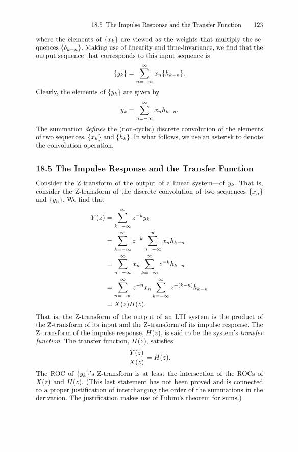
18.5 The Impulse Response and the Transfer Function 123
where the elements of {xk} are viewed as the weights that multiply the se-quences {δk−n}. Making use of linearity and time-invariance, we find that theoutput sequence that corresponds to this input sequence is
{yk} =∞∑
n=−∞xn{hk−n}.
Clearly, the elements of {yk} are given by
yk =∞∑
n=−∞xnhk−n.
The summation defines the (non-cyclic) discrete convolution of the elementsof two sequences, {xk} and {hk}. In what follows, we use an asterisk to denotethe convolution operation.
18.5 The Impulse Response and the Transfer Function
Consider the Z-transform of the output of a linear system—of yk. That is,consider the Z-transform of the discrete convolution of two sequences {xn}and {yn}. We find that
Y (z) =∞∑
k=−∞z−kyk
=∞∑
k=−∞z−k
∞∑
n=−∞xnhk−n
=∞∑
n=−∞xn
∞∑
k=−∞z−khk−n
=∞∑
n=−∞z−nxn
∞∑
k=−∞z−(k−n)hk−n
= X(z)H(z).
That is, the Z-transform of the output of an LTI system is the product ofthe Z-transform of its input and the Z-transform of its impulse response. TheZ-transform of the impulse response, H(z), is said to be the system’s transferfunction. The transfer function, H(z), satisfies
Y (z)X(z)
= H(z).
The ROC of {yk}’s Z-transform is at least the intersection of the ROCs ofX(z) and H(z). (This last statement has not been proved and is connectedto a proper justification of interchanging the order of the summations in thederivation. The justification makes use of Fubini’s theorem for sums.)
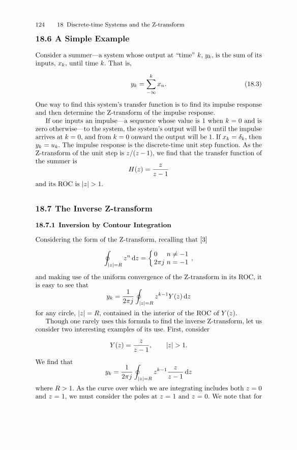
124 18 Discrete-time Systems and the Z-transform
18.6 A Simple Example
Consider a summer—a system whose output at “time” k, yk, is the sum of itsinputs, xk, until time k. That is,
yk =k∑
−∞xn. (18.3)
One way to find this system’s transfer function is to find its impulse responseand then determine the Z-transform of the impulse response.
If one inputs an impulse—a sequence whose value is 1 when k = 0 and iszero otherwise—to the system, the system’s output will be 0 until the impulsearrives at k = 0, and from k = 0 onward the output will be 1. If xk = δk, thenyk = uk. The impulse response is the discrete-time unit step function. As theZ-transform of the unit step is z/(z − 1), we find that the transfer function ofthe summer is
H(z) =z
z − 1and its ROC is |z| > 1.
18.7 The Inverse Z-transform
18.7.1 Inversion by Contour Integration
Considering the form of the Z-transform, recalling that [3]∮
|z|=R
zn dz ={
0 n �= −12πj n = −1 ,
and making use of the uniform convergence of the Z-transform in its ROC, itis easy to see that
yk =1
2πj
∮
|z|=R
zk−1Y (z) dz
for any circle, |z| = R, contained in the interior of the ROC of Y (z).Though one rarely uses this formula to find the inverse Z-transform, let us
consider two interesting examples of its use. First, consider
Y (z) =z
z − 1, |z| > 1.
We find thatyk =
12πj
∮
|z|=R
zk−1 z
z − 1dz
where R > 1. As the curve over which we are integrating includes both z = 0and z = 1, we must consider the poles at z = 1 and z = 0. We note that for
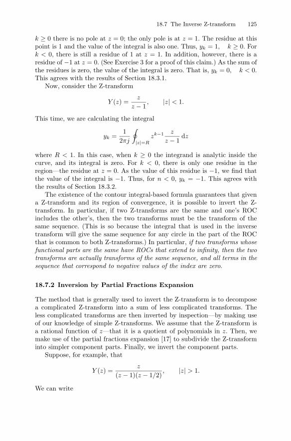
18.7 The Inverse Z-transform 125
k ≥ 0 there is no pole at z = 0; the only pole is at z = 1. The residue at thispoint is 1 and the value of the integral is also one. Thus, yk = 1, k ≥ 0. Fork < 0, there is still a residue of 1 at z = 1. In addition, however, there is aresidue of −1 at z = 0. (See Exercise 3 for a proof of this claim.) As the sum ofthe residues is zero, the value of the integral is zero. That is, yk = 0, k < 0.This agrees with the results of Section 18.3.1.
Now, consider the Z-transform
Y (z) =z
z − 1, |z| < 1.
This time, we are calculating the integral
yk =1
2πj
∮
|z|=R
zk−1 z
z − 1dz
where R < 1. In this case, when k ≥ 0 the integrand is analytic inside thecurve, and its integral is zero. For k < 0, there is only one residue in theregion—the residue at z = 0. As the value of this residue is −1, we find thatthe value of the integral is −1. Thus, for n < 0, yk = −1. This agrees withthe results of Section 18.3.2.
The existence of the contour integral-based formula guarantees that givena Z-transform and its region of convergence, it is possible to invert the Z-transform. In particular, if two Z-transforms are the same and one’s ROCincludes the other’s, then the two transforms must be the transform of thesame sequence. (This is so because the integral that is used in the inversetransform will give the same sequence for any circle in the part of the ROCthat is common to both Z-transforms.) In particular, if two transforms whosefunctional parts are the same have ROCs that extend to infinity, then the twotransforms are actually transforms of the same sequence, and all terms in thesequence that correspond to negative values of the index are zero.
18.7.2 Inversion by Partial Fractions Expansion
The method that is generally used to invert the Z-transform is to decomposea complicated Z-transform into a sum of less complicated transforms. Theless complicated transforms are then inverted by inspection—by making useof our knowledge of simple Z-transforms. We assume that the Z-transform isa rational function of z—that it is a quotient of polynomials in z. Then, wemake use of the partial fractions expansion [17] to subdivide the Z-transforminto simpler component parts. Finally, we invert the component parts.
Suppose, for example, that
Y (z) =z
(z − 1)(z − 1/2), |z| > 1.
We can write
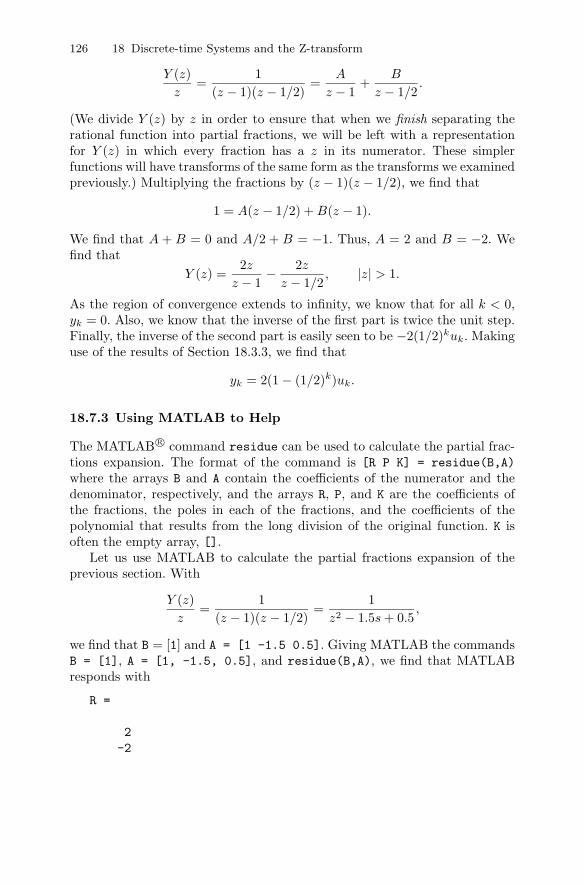
126 18 Discrete-time Systems and the Z-transform
Y (z)z
=1
(z − 1)(z − 1/2)=
A
z − 1+
B
z − 1/2.
(We divide Y (z) by z in order to ensure that when we finish separating therational function into partial fractions, we will be left with a representationfor Y (z) in which every fraction has a z in its numerator. These simplerfunctions will have transforms of the same form as the transforms we examinedpreviously.) Multiplying the fractions by (z − 1)(z − 1/2), we find that
1 = A(z − 1/2) + B(z − 1).
We find that A + B = 0 and A/2 + B = −1. Thus, A = 2 and B = −2. Wefind that
Y (z) =2z
z − 1− 2z
z − 1/2, |z| > 1.
As the region of convergence extends to infinity, we know that for all k < 0,yk = 0. Also, we know that the inverse of the first part is twice the unit step.Finally, the inverse of the second part is easily seen to be −2(1/2)kuk. Makinguse of the results of Section 18.3.3, we find that
yk = 2(1 − (1/2)k)uk.
18.7.3 Using MATLAB to Help
The MATLAB r© command residue can be used to calculate the partial frac-tions expansion. The format of the command is [R P K] = residue(B,A)where the arrays B and A contain the coefficients of the numerator and thedenominator, respectively, and the arrays R, P, and K are the coefficients ofthe fractions, the poles in each of the fractions, and the coefficients of thepolynomial that results from the long division of the original function. K isoften the empty array, [].
Let us use MATLAB to calculate the partial fractions expansion of theprevious section. With
Y (z)z
=1
(z − 1)(z − 1/2)=
1z2 − 1.5s + 0.5
,
we find that B = [1] and A = [1 -1.5 0.5]. Giving MATLAB the commandsB = [1], A = [1, -1.5, 0.5], and residue(B,A), we find that MATLABresponds with
R =
2-2
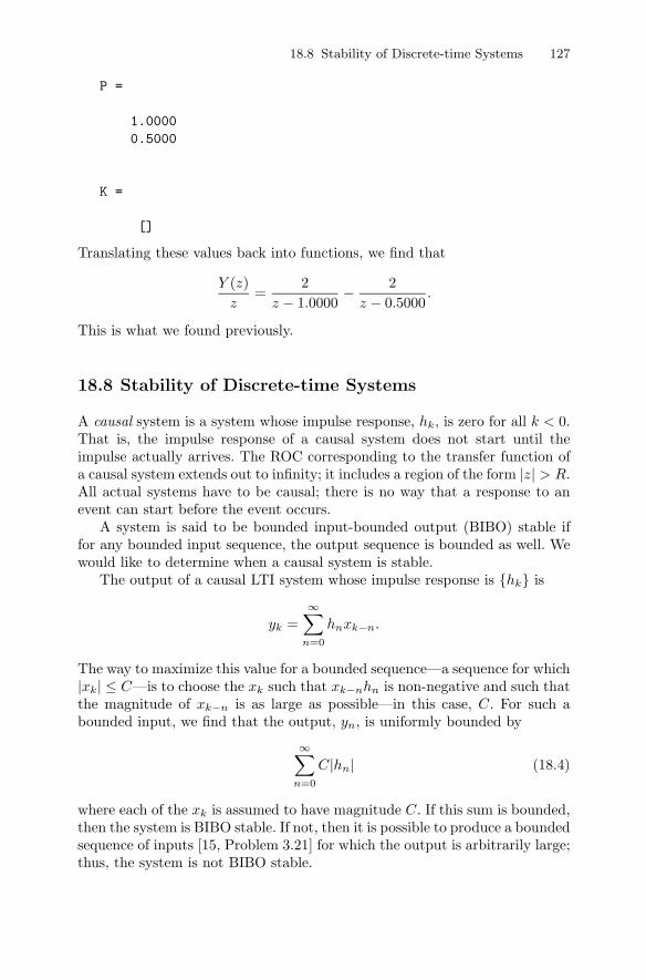
18.8 Stability of Discrete-time Systems 127
P =
1.00000.5000
K =
[]
Translating these values back into functions, we find that
Y (z)z
=2
z − 1.0000− 2
z − 0.5000.
This is what we found previously.
18.8 Stability of Discrete-time Systems
A causal system is a system whose impulse response, hk, is zero for all k < 0.That is, the impulse response of a causal system does not start until theimpulse actually arrives. The ROC corresponding to the transfer function ofa causal system extends out to infinity; it includes a region of the form |z| > R.All actual systems have to be causal; there is no way that a response to anevent can start before the event occurs.
A system is said to be bounded input-bounded output (BIBO) stable iffor any bounded input sequence, the output sequence is bounded as well. Wewould like to determine when a causal system is stable.
The output of a causal LTI system whose impulse response is {hk} is
yk =∞∑
n=0
hnxk−n.
The way to maximize this value for a bounded sequence—a sequence for which|xk| ≤ C—is to choose the xk such that xk−nhn is non-negative and such thatthe magnitude of xk−n is as large as possible—in this case, C. For such abounded input, we find that the output, yn, is uniformly bounded by
∞∑
n=0
C|hn| (18.4)
where each of the xk is assumed to have magnitude C. If this sum is bounded,then the system is BIBO stable. If not, then it is possible to produce a boundedsequence of inputs [15, Problem 3.21] for which the output is arbitrarily large;thus, the system is not BIBO stable.
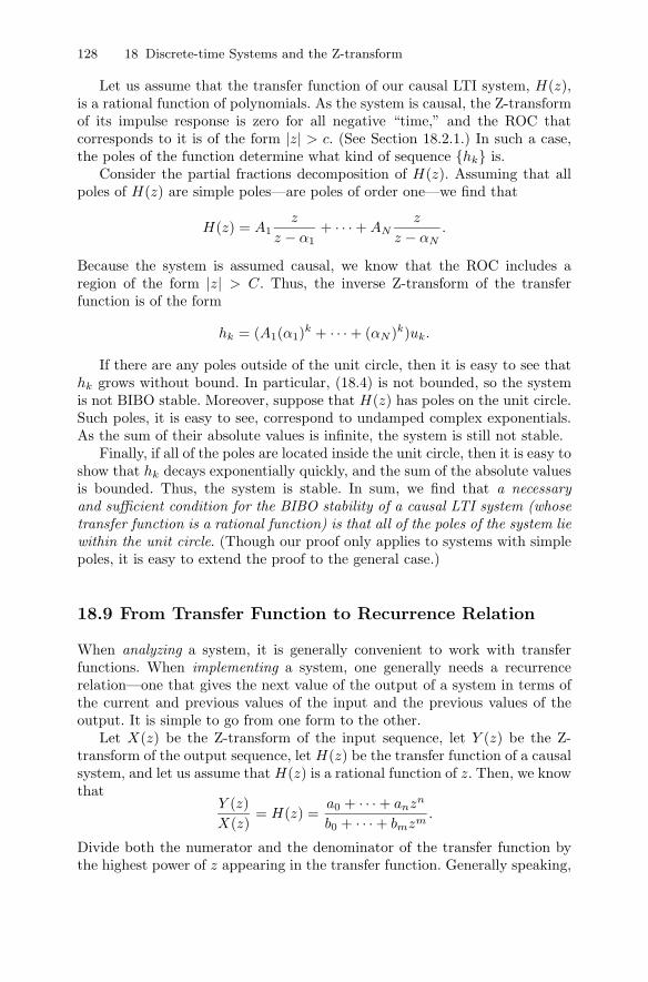
128 18 Discrete-time Systems and the Z-transform
Let us assume that the transfer function of our causal LTI system, H(z),is a rational function of polynomials. As the system is causal, the Z-transformof its impulse response is zero for all negative “time,” and the ROC thatcorresponds to it is of the form |z| > c. (See Section 18.2.1.) In such a case,the poles of the function determine what kind of sequence {hk} is.
Consider the partial fractions decomposition of H(z). Assuming that allpoles of H(z) are simple poles—are poles of order one—we find that
H(z) = A1z
z − α1+ · · · + AN
z
z − αN.
Because the system is assumed causal, we know that the ROC includes aregion of the form |z| > C. Thus, the inverse Z-transform of the transferfunction is of the form
hk = (A1(α1)k + · · · + (αN )k)uk.
If there are any poles outside of the unit circle, then it is easy to see thathk grows without bound. In particular, (18.4) is not bounded, so the systemis not BIBO stable. Moreover, suppose that H(z) has poles on the unit circle.Such poles, it is easy to see, correspond to undamped complex exponentials.As the sum of their absolute values is infinite, the system is still not stable.
Finally, if all of the poles are located inside the unit circle, then it is easy toshow that hk decays exponentially quickly, and the sum of the absolute valuesis bounded. Thus, the system is stable. In sum, we find that a necessaryand sufficient condition for the BIBO stability of a causal LTI system (whosetransfer function is a rational function) is that all of the poles of the system liewithin the unit circle. (Though our proof only applies to systems with simplepoles, it is easy to extend the proof to the general case.)
18.9 From Transfer Function to Recurrence Relation
When analyzing a system, it is generally convenient to work with transferfunctions. When implementing a system, one generally needs a recurrencerelation—one that gives the next value of the output of a system in terms ofthe current and previous values of the input and the previous values of theoutput. It is simple to go from one form to the other.
Let X(z) be the Z-transform of the input sequence, let Y (z) be the Z-transform of the output sequence, let H(z) be the transfer function of a causalsystem, and let us assume that H(z) is a rational function of z. Then, we knowthat
Y (z)X(z)
= H(z) =a0 + · · · + anzn
b0 + · · · + bmzm.
Divide both the numerator and the denominator of the transfer function bythe highest power of z appearing in the transfer function. Generally speaking,
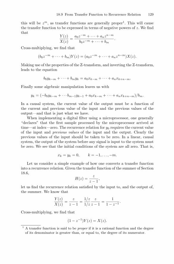
18.9 From Transfer Function to Recurrence Relation 129
this will be zm, as transfer functions are generally proper1. This will causethe transfer function to be expressed in terms of negative powers of z. We findthat
Y (z)X(z)
=a0z
−m + · · · + anzn−m
b0z−m + · · · + bm.
Cross-multiplying, we find that
(b0z−m + · · · + bm)Y (z) = (a0z
−m + · · · + anzn−m)X(z).
Making use of the properties of the Z-transform, and inverting the Z-transform,leads to the equation
b0yk−m + · · · + bmyk = a0xk−m + · · · + anxk+n−m.
Finally some algebraic manipulation leaves us with
yk = (−b0yk−m + · · · bm−1yk−1 + a0xk−m + · · · + anxk+n−m)/bm.
In a causal system, the current value of the output must be a function ofthe current and previous value of the input and the previous values of theoutput—and that is just what we have.
When implementing a digital filter using a microprocessor, one generally“declares” that the first sample processed by the microprocessor arrived attime—at index—zero. The recurrence relation for y0 requires the current valueof the input and previous values of the input and the output. Clearly theprevious values of the input should be taken to be zero. In a linear, causalsystem, the output of the system before any signal is input to the system mustbe zero. We see that the initial conditions of the system are all zero. That is,
xk = yk = 0, k = −1, . . . ,−m.
Let us consider a simple example of how one converts a transfer functioninto a recurrence relation. Given the transfer function of the summer of Section18.6,
H(z) =z
z − 1,
let us find the recurrence relation satisfied by the input to, and the output of,the summer. We know that
Y (z)X(z)
=z
z − 1=
1/z
1/z
z
z − 1=
11 − z−1
.
Cross-multiplying, we find that
(1 − z−1)Y (z) = X(z).1 A transfer function is said to be proper if it is a rational function and the degree
of its denominator is greater than, or equal to, the degree of its numerator.
130 18 Discrete-time Systems and the Z-transform
Converting back to an equation in the time domain, we find that
yk − yk−1 = xk ⇒ yk = xk + yk−1.
Considering (18.3) and noting that
yk−1 =k−1∑
n=−∞xn,
we find that our recurrence relation is indeed satisfied by the output of thesummer.
18.10 The Sinusoidal Steady-state Response ofDiscrete-time Systems
Consider a stable LTI system whose transfer function is H(z). Suppose thatthe system accepts samples that are taken every T seconds. If the input tothe system is a complex exponential with angular frequency ω = 2πf , thesamples seen by the system are
xk ={
ejωkT k ≥ 00 k < 0 .
As the non-zero terms are of the form αk for α = ejωT , the Z-transform ofthis sequence is simply
X(z) =z
z − ejωT.
The Z-transform of the output of the system, Y (z), is
Y (z) = H(z)z
z − ejωT.
Consider the partial fractions expansion of the output. It contains two setsof terms. One term has the same pole as the input. All the rest “inherit” thepoles of H(z)—all of which lie inside the unit circle.
Consider the inverse Z-transform of Y (z). All the terms whose poles areinherited from the transfer function correspond to damped exponentials. Thus,in the steady state they make no contribution. In order to determine thesteady-state behavior, we need only know the coefficient of
z
z − ejωT.
Let us calculate this coefficient.We know that
Y (z) = H(z)z
z − ejωT=
Az
z − ejωT+ poles inside unit circle.
18.10 The Sinusoidal Steady-state Response of Discrete-time Systems 131
Multiplying through by z − ejωT and substituting z = ejωT , we find that
A = H(ejωT ).
The sinusoidal steady-state response—the response after all the transientshave died down—is H(ejωT ) times the input complex sinusoid.
If the input to the system is
xk ={
cos(ωkT ) k ≥ 00 k < 0,
then by using Euler’s formula and the linearity of the Z-transform, we findthat the steady-state response is
12[H(ejωT )ejωkT + H(e−jωT )e−jωkT
].
As long as the polynomials that define H(z) have real coefficients, it is easyto show that H(z) = H(z). Thus, we find that the steady-state output is
steady-state output =12(H(ejωT )ejωkT + H(e−jωT )e−jωkT
)
=12
(H(ejωT )ejωkT + H(ejωT )ejωkT
)
= Re(H(ejωT )ejωkT )= Re(H(ejωT )) cos(ωkT ) − Im(H(ejωT )) sin(ωT ).
This is easily seen to be equal to
|H(ejωT )| cos{ωkT + � [H(ejωT )]}.
That is, the system filters the input sinusoid. It amplifies it in a way that isdependent on ω and it shifts its phase in a way that is dependent on ω.
The function H(ejωT ) is called the frequency response of the system and|H(ejωT )| is known as the system’s magnitude response. Note that the fre-quency (and magnitude) response is a periodic function of ω whose period is2π/T . (This is perfectly reasonable, as sampling a signal aliases frequenciesabove f = 1/(2T )—or ω = π/T—to frequencies below f = 1/(2T ).) Let ustake the region ω ∈ (−π/T, π/T ] as the period of interest. Assuming that thepolynomials of which H(z) is composed have real coefficients, we know thatH(e−jωT ) = H(ejωT ). Thus, the negative frequencies do not provide any newinformation. In order to understand the entire frequency response, it is suf-ficient to know the frequency response in the region ω ∈ [0, π/T ]. Generallyspeaking, when a frequency (or magnitude) response is plotted, it is only plot-ted in this range. (The angular frequency π/T corresponds to the frequency1/(2T )—the Nyquist frequency of the system.)
132 18 Discrete-time Systems and the Z-transform
18.11 MATLAB and Linear Time-invariant Systems
MATLAB has two “levels” of commands for helping users analyze and designlinear time-invariant systems. One set of commands are standard command-line functions that allow the user to define an LTI system and perform differentanalyses on LTI systems. The second “class” of functions is a single commandthat opens a graphical user interface that allows the user to perform manyanalyses from within a single window.
18.11.1 Individual Commands
Before one can analyze an LTI using MATLAB, one must define the LTI forMATLAB. MATLAB has a command, tf, for defining a transfer functionobject. Assuming that one would like to describe the discrete-time system
H(z) =aNzN + · · · + a0
bMzM + · · · + b0
whose sampling time is Ts, one gives MATLAB the command
H = tf([aN aN−1 . . . a0], [bM bM−1 . . . b0], Ts).
If one does not wish to specify a sampling time, then in place of Ts one enters−1.
Suppose, for example, that one wanted to characterize a summer to MAT-LAB, and suppose that the sampling period of the system is 1ms. Assumingthat one wants to refer to the transfer function as H, one would give MAT-LAB the command H = tf([1 0],[1 -1], 0.001). MATLAB replies to thiscommand with
Transfer function:z
-----z - 1
Sampling time: 0.001
Having defined the system to MATLAB, it is now simple to have MATLABprovide all sorts of information about the system. Perhaps the most commonlyused function is bode. This command causes MATLAB to produce the Bodeplots2 that correspond to a system. As we have mentioned, it is common toplot the frequency response up to the angular frequency π/T .2 The Bode plots that correspond to a system are plots of the system’s magnitude
response and the system’s phase response. The magnitude response is generallygiven in dB, and the frequency axis is logarithmic. The phase response is givenin degrees, and the frequency axis is logarithmic. The plots are generally givenone above the other, with the frequency axes scaled identically.
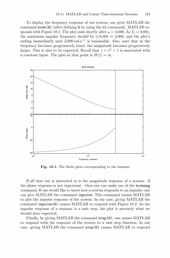
18.11 MATLAB and Linear Time-invariant Systems 133
To display the frequency response of our system, one gives MATLAB thecommand bode(H) (after defining H by using the tf command). MATLAB re-sponds with Figure 18.1. The plot ends shortly after ω = 3,000. As Ts = 0.001,the maximum angular frequency should be π/0.001 ≈ 3,000, and the plot’sending immediately past 3,000 rad s−1 is reasonable. Also, note that as thefrequency becomes progressively lower, the magnitude becomes progressivelylarger. This is also to be expected. Recall that z = e0 = 1 is associated witha constant input. The gain at that point is H(1) = ∞.
−10
−5
0
5
10
15
20
25
Mag
nitu
de (
dB)
102
103
104
−90
−45
0
45
Pha
se (
deg)
Bode Diagram
Frequency (rad/sec)
Fig. 18.1. The Bode plots corresponding to the summer
If all that one is interested in is the magnitude response of a system—ifthe phase response is not important—then one can make use of the bodemagcommand. If one would like to know how a system responds to an impulse, onecan give MATLAB the command impulse. This command causes MATLABto plot the impulse response of the system. In our case, giving MATLAB thecommand impulse(H) causes MATLAB to respond with Figure 18.2. As theimpulse response of a summer is a unit step, the plot is precisely what weshould have expected.
Finally, by giving MATLAB the command step(H), one causes MATLABto respond with the response of the system to a unit step function. In ourcase, giving MATLAB the command step(H) causes MATLAB to respond
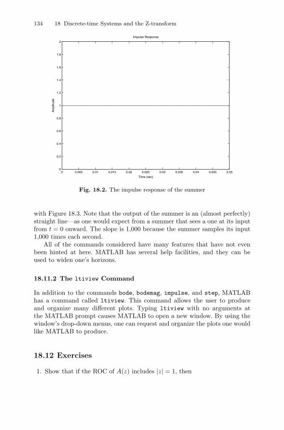
134 18 Discrete-time Systems and the Z-transform
0 0.005 0.01 0.015 0.02 0.025 0.03 0.035 0.04 0.045 0.050
0.2
0.4
0.6
0.8
1
1.2
1.4
1.6
1.8
2
Impulse Response
Time (sec)
Am
plitu
de
Fig. 18.2. The impulse response of the summer
with Figure 18.3. Note that the output of the summer is an (almost perfectly)straight line—as one would expect from a summer that sees a one at its inputfrom t = 0 onward. The slope is 1,000 because the summer samples its input1,000 times each second.
All of the commands considered have many features that have not evenbeen hinted at here. MATLAB has several help facilities, and they can beused to widen one’s horizons.
18.11.2 The ltiview Command
In addition to the commands bode, bodemag, impulse, and step, MATLABhas a command called ltiview. This command allows the user to produceand organize many different plots. Typing ltiview with no arguments atthe MATLAB prompt causes MATLAB to open a new window. By using thewindow’s drop-down menus, one can request and organize the plots one wouldlike MATLAB to produce.
18.12 Exercises
1. Show that if the ROC of A(z) includes |z| = 1, then
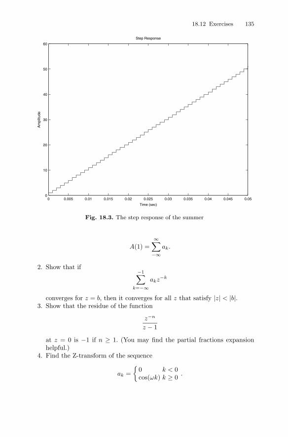
18.12 Exercises 135
0 0.005 0.01 0.015 0.02 0.025 0.03 0.035 0.04 0.045 0.050
10
20
30
40
50
60
Step Response
Time (sec)
Am
plitu
de
Fig. 18.3. The step response of the summer
A(1) =∞∑
−∞ak.
2. Show that if−1∑
k=−∞akz−k
converges for z = b, then it converges for all z that satisfy |z| < |b|.3. Show that the residue of the function
z−n
z − 1
at z = 0 is −1 if n ≥ 1. (You may find the partial fractions expansionhelpful.)
4. Find the Z-transform of the sequence
ak ={
0 k < 0cos(ωk) k ≥ 0 .
136 18 Discrete-time Systems and the Z-transform
5. Prove that the Z-transform is linear by making use of the definition ofthe Z-transform. Also, show that the ROC of the resulting Z-transformcontains the intersection of the ROCs of the two transforms whose com-bination is being taken.
6. Find the Z-transform of the sequence
ak ={
0 k < 0k k ≥ 0 .
7. Let
ak ={
1/k k ≥ 10 k < 1 .
Show that the sum that defines A(1) diverges while the sum that definesA(−1) converges conditionally. Show that this implies that the ROC ofthe Z-transform contains the region |z| > 1, and explain in what sense thebehavior of A(z) is “odd” on the circle |z| = 1.
8. Suppose that the functions below are taken to be the transfer functionsof causal systems. Which of the functions correspond to stable systems?a)
H(z) =z
z2 + 1.
b)
H(z) =z
z + 1/2.
c)
H(z) =z
z − 1/2.
d)
H(z) =z
z2 − z/2 + 1/4.
9. Find the sequence that corresponds to each of the following Z-transformsa)
H(z) =z
(z − 1/2)(z + 1/2), |z| > 1/2.
b)
H(z) =z
(z − 1/2)2, |z| > 1/2.
c)
H(z) =z
(z − 1/2)2, |z| < 1/2.
18.12 Exercises 137
10. Find the Z-transforms of the following sequencesa)
{ak} = {0, 0, . . . , 0, 1, . . . , k2, . . .} = {k2uk}.b)
{ak} = {. . . , 1/2, 1, 1/2, . . . , } ={
12|k|
}.
11. Sketch the magnitude response of the filter whose transfer function is
H(z) =z
z − 1/2.
Check your answer using the MATLAB bodemag command. (You will needto set Ts = −1 in the tf command.)
12. Calculate the Z-transform of the sequence {δk}.13. Find the recurrence relation that corresponds to the causal systems de-
scribed by each of the following transfer functions. Let the sequence inputto the system be xk and the sequence output by the system be yk.a)
H(z) =z
z2 − 1.
b)
H(z) =z − 1/2
z2 − z/2 − 1/2.
14. Calculate the inverse Z-transform of
A(z) =z
z − α, |z| < α.
You may wish to write the function as a Taylor series in power of z/α.
19
Filter Types
Summary. Analog filters are generally built using resistors, capacitors, inductors,and operational amplifiers. The impulse response of such filters begins when theimpulse arrives and continues indefinitely. A filter with an impulse response of thistype is known as an infinite impulse response (IIR) filter.
In this chapter, we discuss the filter types available to the engineer designingdigital filters. Some digital filters are IIR filters, while others are finite impulseresponse (FIR) filters. An FIR filter is a filter whose impulse response is identicallyzero after a certain time.
Keywords. impulse response, IIR, FIR.
19.1 Finite Impulse Response Filters
Suppose that the impulse response of a digital filter is
hn, |n| ≤ N,
and is zero for all n outside of this range. Filters of this sort—filters whoseimpulse response consists of a finite number of terms—are called finite impulseresponse (FIR) filters. By making use of the principle of superposition, it iseasy to see that the response, yn, of the filter to a generic signal xn is
yn =∞∑
k=−∞xkhn−k
= xn−NhN + xn−(N−1)hN−1 + · · · + xnh0 + · · · + h−Nxn+N .
That is, yn is a weighted sum of samples of the input. The transfer functionof an FIR filter can be expressed as
H(z) = h−NzN + · · · + h−1z1 + h0 + h1z
−1 + · · · + hNz−N
=z2Nh−N + · · · + zNh0 + · · · + hN
zN, 0 < |z| < ∞.
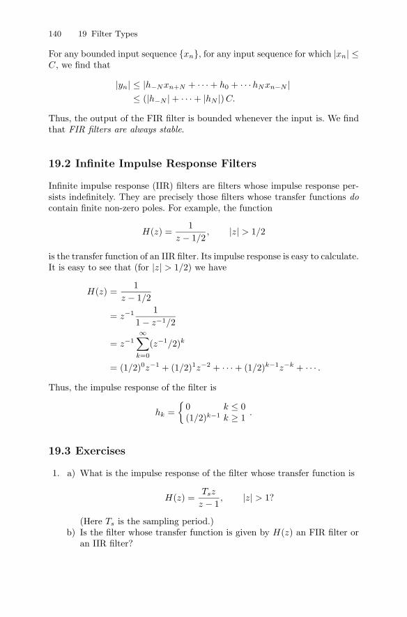
140 19 Filter Types
For any bounded input sequence {xn}, for any input sequence for which |xn| ≤C, we find that
|yn| ≤ |h−Nxn+N + · · · + h0 + · · ·hNxn−N |≤ (|h−N | + · · · + |hN |) C.
Thus, the output of the FIR filter is bounded whenever the input is. We findthat FIR filters are always stable.
19.2 Infinite Impulse Response Filters
Infinite impulse response (IIR) filters are filters whose impulse response per-sists indefinitely. They are precisely those filters whose transfer functions docontain finite non-zero poles. For example, the function
H(z) =1
z − 1/2, |z| > 1/2
is the transfer function of an IIR filter. Its impulse response is easy to calculate.It is easy to see that (for |z| > 1/2) we have
H(z) =1
z − 1/2
= z−1 11 − z−1/2
= z−1∞∑
k=0
(z−1/2)k
= (1/2)0z−1 + (1/2)1z−2 + · · · + (1/2)k−1z−k + · · · .Thus, the impulse response of the filter is
hk ={
0 k ≤ 0(1/2)k−1 k ≥ 1 .
19.3 Exercises
1. a) What is the impulse response of the filter whose transfer function is
H(z) =Tsz
z − 1, |z| > 1?
(Here Ts is the sampling period.)b) Is the filter whose transfer function is given by H(z) an FIR filter or
an IIR filter?

19.3 Exercises 141
c) Find the filter’s output, yk, as a function of its input, xk. You mayassume that xk = 0 for all k < 0.
d) What operation does this filter approximate when Ts << 1?2. What is the impulse response of the filter defined by
H(z) =z
z + 1/2, |z| > 1/2?
Is this filter an FIR or an IIR filter? Explain!3. What is the impulse response of the filter defined by
H(z) =z
z + 1/2, |z| < 1/2?
Is this filter an FIR or an IIR filter? Explain!
20
When to Use C (Rather than AssemblyLanguage)
Summary. In many introductory microprocessor (or microcontroller) courses, oneis taught to program in assembly language. Until now, it was probably best toprogram in assembly language, but at this point it is probably best to move to C.In this chapter, we discuss why one might want to make this change, and we give afirst example of implementing a filter using a program written in C.
Keywords. assembly language, C, low-pass filter, RC filter.
20.1 Introduction
In introductory courses in microprocessors, one often spends much of one’stime controlling the processor and its peripherals. Assembly language is builtfor such tasks and makes them relatively easy. In particular, the machinelanguage of the 8051 family of microprocessors supports many instructionsthat work on individual bits. When every bit is significant—as it is when oneis setting up an SFR—this ability is very important.
In several of the early laboratories, we used a microprocessor as a data-gathering tool. We set up its SFRs and let the microprocessor run. In such acase, it makes sense to use assembly language. In the laboratories that follow,we use the microprocessor (often a microcontroller) to do calculations. Whenone is interested in relatively heavy-duty calculations, it often makes senseto move to a high-level language. In our case, that language is C. For moreinformation about the version of C we used with the ADuC841, see [13].
20.2 A Simple Low-pass Filter
In order to make the first C program relatively simple, we consider a simpleinfinite impulse response (IIR) filter. Perhaps the simplest IIR digital filter isthe (causal) filter defined by the equation
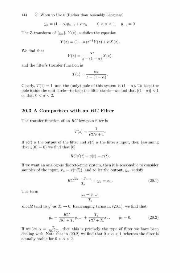
144 20 When to Use C (Rather than Assembly Language)
yn = (1 − α)yn−1 + αxn, 0 < α < 1, y−1 = 0.
The Z-transform of {yn}, Y (z), satisfies the equation
Y (z) = (1 − α)z−1Y (z) + αX(z).
We find thatY (z) =
αz
z − (1 − α)X(z),
and the filter’s transfer function is
T (z) =αz
z − (1 − α).
Clearly, T (1) = 1, and the (only) pole of this system is (1 − α). To keep thepole inside the unit circle—to keep the filter stable—we find that |(1−α)| < 1or that 0 < α < 2.
20.3 A Comparison with an RC Filter
The transfer function of an RC low-pass filter is
T (s) =1
RCs + 1.
If y(t) is the output of the filter and x(t) is the filter’s input, then (assumingthat y(0) = 0) we find that [6]
RCy′(t) + y(t) = x(t).
If we want an analogous discrete-time system, then it is reasonable to considersamples of the input, xn = x(nTs), and to let the output, yn, satisfy
RCyn − yn−1
Ts+ yn = xn. (20.1)
The termyn − yn−1
Ts
should tend to y′ as Ts → 0. Rearranging terms in (20.1), we find that
yn =RC
RC + Tsyn−1 +
Ts
RC + Tsxn, y0 = 0. (20.2)
If we let α = TsRC+Ts
, then this is precisely the type of filter we have beendealing with. Note that in (20.2) we find that 0 < α < 1, whereas the filter isactually stable for 0 < α < 2.
20.5 Exercises 145
20.4 The Experiment
Write a C program to implement the filter of Section 20.2. It should be possibleto achieve a sample rate of 5,000 samples s−1. Try a variety of values of α.Make sure that some of the values exceed one. For a square wave input, whatdoes the output look like when α < 1? What about when α > 1? In whatway(s) is the output when α > 1 similar to the output of a standard RClow-pass filter? In what way(s) is it different?
Compare the C code with the computer-generated assembly language code.(To cause the computer to include the assembly code in the listing when usingthe Keil μVision3 IDE, you must change the options for the project.) Note thatin the sections where one is setting up the registers, the assembly languagecode is not much longer than the C code. However, in the regions where the Ccode is performing calculations, the assembly language code is much longer.
20.5 Exercises
1. Find and plot the magnitude response of the filter described in Section20.2 when α = 3/2.
2. Find the impulse response of the causal filter whose transfer function is
T (z) =αz
z − (1 − α), 0 < α < 2.
What qualitative change does the impulse response undergo when α goesfrom being less than one to being more than one?
3. Show that for 1 < α < 2, the causal filter whose transfer function is
T (z) =αz
z − (1 − α)
is a high-pass filter.4. a) Use Simulink r© to simulate the “RC-type” filter of Sections 20.2 and
20.3 for a variety of values of 0 < α < 1 and 1 < α < 2. Let thesampling period be 0.01 s.
b) Examine the filter’s response to a variety of low- and high-frequencysinewaves both when the system includes an anti-aliasing filter andwhen it does not.
c) Use the MATLAB command bode to examine the frequency responseof the filters that were implemented. To what extent do the simulationresults agree with the information presented on the Bode plots?
21
Two Simple FIR Filters
Summary. Having seen (and implemented) a simple IIR filter, we consider twosimple FIR filters. In this chapter, we develop both a simple FIR low-pass filter anda simple FIR high-pass filter.
Keywords. averaging filter, high-pass filter, low-pass filter, FIR filters.
21.1 Introduction
The averaging filter is a simple finite impulse response (FIR) low-pass filter.Let Fs be the sampling rate of the system, and let Ts be its reciprocal, thesampling period. Let xk = x(kTs) be the kth sample of the input (where kstarts from 0), and let yk be the output of the filter at time t = kTs. Then,an N -coefficient (also known as an N -tap) low-pass filter is defined by theequation
yn =xn + xn−1 + · · · + xn−N+1
N.
This filter’s output, yn, is the running average of the last N samples of theinput, xn.
The Z-transform of the sequence {yn} is
Y (z) = (1 + z−1 + · · · + z−N+1)X(z)/N. (21.1)
Summing the finite geometric series, we find that the transfer function of thefilter, TLP(z), is
TLP(z) =1N
1 − z−N
1 − z−1.
Substituting z = e2πjfTs , we find that the frequency response of the filter is
148 21 Two Simple FIR Filters
TLP(e2πjfTs) =1N
1 − e−2NπjfTs
1 − e−2πjfTs
=1N
e−(N−1)πjfTssin(NπfTs)sin(πfTs)
.
Making use of L’hopital’s rule (or, more properly, not using the formula forthe geometric series when f = k/Ts but simply summing the series), we findthat at f = 0 the transfer function is 1; at no other point is it greater. (SeeExercise 3.)
The simplest FIR high-pass filter is given by the equation
yn =1N
(xn − xn−1 + · · · + (−1)kxn−k + · · · − xn−N+1
)
where N is even. Passing to the Z-transform of {yn}, Y (z), we find that
Y (z) =1N
(1 − z−1 + · · · + (−1)kz−k + · · · − z−N+1
)X(z).
The transfer function of the filter, THP(z), is
THP(z) =1N
(1 − z−1 + · · · + (−1)kz−k + · · · − z−N+1
)
=1N
1 − (−1)Nz−N
1 + z−1. (21.2)
As by assumption N is even, we find that
THP(z) =1N
1 − z−N
1 + z−1.
Substituting z = e2πjfTs , we find that the frequency response of the filter is
THP(e2πjfTs) =1N
1 − e−2NπjfTs
1 + e−2πjfTs
=1N
e−NπjfTs
e−πjfTs
eNπjfTs − e−NπjfTs
eπjfTs + e−πjfTs
=1N
e−(N−1)πjfTsjsin(NπfTs)cos(πfTs)
.
Note that when f = 0, the frequency response of this filter is zero. The filterdoes not pass DC at all. Plugging z = e2πj(1/(2Ts))Ts = −1 into (21.2), it iseasy to see that when f = 1/(2Ts)—which is the “Nyquist frequency” for thefilter—the filter’s frequency response is 1. In the sinusoidal steady state, thefilter passes high-frequency signals without altering them.
21.3 Exercises 149
21.2 The Experiment
Please modify the program that implements a simple IIR filter to implementthe simple averaging filter with five elements in the average. A sample rate of5,000 samples s−1 should be achievable. Note that there is no need to buffer thesamples of the output—they are never reused. (That is an essential differencebetween FIR and IIR filters.)
Please examine the frequency response of the filter. Use a sinewave gener-ator and an oscilloscope. Does practice agree with theory?
Having finished with the averaging filter, implement the simple high-passfilter with N = 6. Once again, a sample rate of 5,000 samples s−1 shouldbe achievable. Using a sinewave generator and an oscilloscope, examine thefilter’s frequency response. Do practice and theory agree?
21.3 Exercises
1. Consider a simple averaging filter with five taps—when N = 5.a) Plot the magnitude response of the filter as a function of fTs.b) At what frequencies do the zeros of the transfer function occur?c) Give an intuitive explanation of the answer to the previous section.
2. Consider the six-tap high-pass filter—the filter for which N = 6.a) Plot the magnitude response of the filter as a function of fTs.b) At what frequencies do the zeros of the transfer function occur?c) Give an intuitive explanation of the answer to the previous section for
at least one of the zeros of the transfer function.3. Make use of (21.1), the triangle inequality, and the definition of the fre-
quency response to show that
|TLP(e2πjfTs)| ≤ 1.
22
Very-narrow-band Filters
Summary. In the preceding chapter, two simple FIR filters were presented. In thischapter, we consider an IIR bandpass filter. In the design of the IIR bandpass filter, asimple FIR notch filter is used. By adding feedback to the system, a programmable-bandwidth IIR filter is produced.
Keywords. notch filter, programmable-bandwidth filter, feedback.
22.1 A Very Simple Notch Filter
Consider the FIR filter whose transfer function is
Tsimple(z) = (1− e2πjFTsz−1)(1− e−2πjFTsz−1) = 1− 2z−1 cos(2πFTs) + z−2.
It is clear that the frequency response of this filter has exactly two zeros, andthey are located at z = e±2πjFTs . That is, this filter has a “notch”—a zero inits frequency response—at ±F Hz.
22.2 From Simple Notch to Effective Bandpass
Consider the system of Figure 22.1. Clearly,
Vout(z) = Vin(z) − KTsimple(z)Vout(z).
Manipulating this equation allows us to show that the transfer function of thesystem with feedback is
Tfeedback(z) =Vout(z)Vin(z)
=1
1 + KTsimple(z).
Tsimple(z) has only the two zeros found above. Thus, when f = ±F Hz, thefrequency response is 1. If K is sufficiently large, it is easy to see that at all
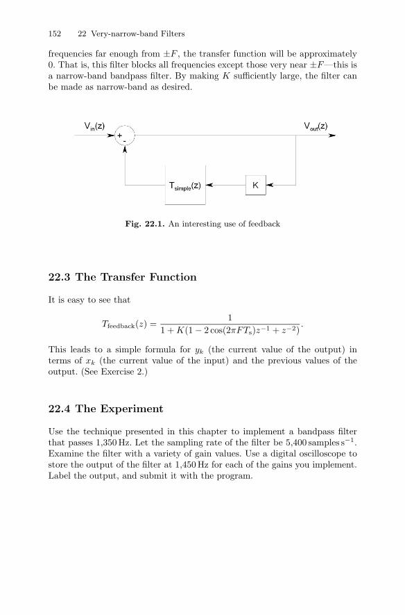
152 22 Very-narrow-band Filters
frequencies far enough from ±F , the transfer function will be approximately0. That is, this filter blocks all frequencies except those very near ±F—this isa narrow-band bandpass filter. By making K sufficiently large, the filter canbe made as narrow-band as desired.
Fig. 22.1. An interesting use of feedback
22.3 The Transfer Function
It is easy to see that
Tfeedback(z) =1
1 + K(1 − 2 cos(2πFTs)z−1 + z−2).
This leads to a simple formula for yk (the current value of the output) interms of xk (the current value of the input) and the previous values of theoutput. (See Exercise 2.)
22.4 The Experiment
Use the technique presented in this chapter to implement a bandpass filterthat passes 1,350 Hz. Let the sampling rate of the filter be 5,400 samples s−1.Examine the filter with a variety of gain values. Use a digital oscilloscope tostore the output of the filter at 1,450 Hz for each of the gains you implement.Label the output, and submit it with the program.
22.5 Exercises 153
22.5 Exercises
1. Explain why putting KTsimple(z) in the “forward path” (in the upperportion of the system), rather than in the feedback loop, gives a notchfilter that removes F Hz signals. (Give a reasonably intuitive explanation.)
2. Find the equation that expresses the output of the filter described in thischapter in terms of the filter’s previous outputs and the filter’s currentand previous inputs.
3. Show that the filter of Section 22.3 is stable for all K > 0.4. Examine the magnitude response of the effective bandpass filter when
K = 10, F = 1 kHz, and Ts = 1/5,400 s. Note that the maximum valueof the magnitude is not 0 dB, and it does not occur at precisely 1 kHz.Explain how this can happen and why this does not contradict the theorydeveloped in this chapter.
23
Design of IIR Digital Filters: TheOld-fashioned Way
Summary. In this chapter, we discuss a systematic method of designing low-passinfinite impulse response (IIR) digital filters. As this procedure requires that onefirst design an analog low-pass filter, we start by discussing the properties of analoglow-pass filters, and we proceed to techniques for designing such filters. Then, weconsider one technique for converting such filters into digital low-pass filters.
Keywords. analog filters, Butterworth filter, Chebyshev filter, elliptic filter, bilinear
transform.
23.1 Analog Filter Design
There are three very standard types of analog filters: Butterworth filters,Chebyshev filters, and elliptic filters. As this is not a course in analog filterdesign, we only describe the filters briefly.
Butterworth filters are also called “maximally flat” filters. The square ofthe magnitude of a low-pass Butterworth filter satisfies the equation
|HB(jω)|2 =1
1 + (jω/jωc)2N.
By making use of the fact that for small |x| we know that 1/(1 + x) ≈ 1 − x,we find that near ω = 0 we can approximate the square of the magnitude by
|HB(jω)|2 ≈ 1 − (ω/ωc)2N .
For values of ω that are much smaller than ωc, this is very close to one. Thefilter is very flat near ω = 0.
Chebyshev filters have the form
|HC(jω)|2 =1
1 + ε2V 2N (ω/ωc)
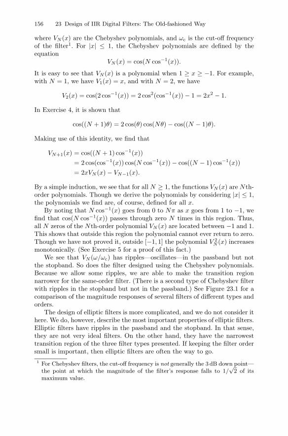
156 23 Design of IIR Digital Filters: The Old-fashioned Way
where VN (x) are the Chebyshev polynomials, and ωc is the cut-off frequencyof the filter1. For |x| ≤ 1, the Chebyshev polynomials are defined by theequation
VN (x) = cos(N cos−1(x)).
It is easy to see that VN (x) is a polynomial when 1 ≥ x ≥ −1. For example,with N = 1, we have V1(x) = x, and with N = 2, we have
V2(x) = cos(2 cos−1(x)) = 2 cos2(cos−1(x)) − 1 = 2x2 − 1.
In Exercise 4, it is shown that
cos((N + 1)θ) = 2 cos(θ) cos(Nθ) − cos((N − 1)θ).
Making use of this identity, we find that
VN+1(x) = cos((N + 1) cos−1(x))= 2 cos(cos−1(x)) cos(N cos−1(x)) − cos((N − 1) cos−1(x))= 2xVN (x) − VN−1(x).
By a simple induction, we see that for all N ≥ 1, the functions VN (x) are Nth-order polynomials. Though we derive the polynomials by considering |x| ≤ 1,the polynomials we find are, of course, defined for all x.
By noting that N cos−1(x) goes from 0 to Nπ as x goes from 1 to −1, wefind that cos(N cos−1(x)) passes through zero N times in this region. Thus,all N zeros of the Nth-order polynomial VN (x) are located between −1 and 1.This shows that outside this region the polynomial cannot ever return to zero.Though we have not proved it, outside [−1, 1] the polynomial V 2
N (x) increasesmonotonically. (See Exercise 5 for a proof of this fact.)
We see that VN (ω/ωc) has ripples—oscillates—in the passband but notthe stopband. So does the filter designed using the Chebyshev polynomials.Because we allow some ripples, we are able to make the transition regionnarrower for the same-order filter. (There is a second type of Chebyshev filterwith ripples in the stopband but not in the passband.) See Figure 23.1 for acomparison of the magnitude responses of several filters of different types andorders.
The design of elliptic filters is more complicated, and we do not consider ithere. We do, however, describe the most important properties of elliptic filters.Elliptic filters have ripples in the passband and the stopband. In that sense,they are not very ideal filters. On the other hand, they have the narrowesttransition region of the three filter types presented. If keeping the filter ordersmall is important, then elliptic filters are often the way to go.1 For Chebyshev filters, the cut-off frequency is not generally the 3 dB down point—
the point at which the magnitude of the filter’s response falls to 1/√
2 of itsmaximum value.
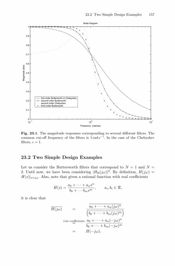
23.2 Two Simple Design Examples 157
10−1
100
101
0
0.1
0.2
0.3
0.4
0.5
0.6
0.7
0.8
0.9
1
Mag
nitu
de (
abs)
first order Butterworth or Chebyshevsecond order Butterworthsecond order Chebyshevthird order Butterworth
Bode Diagram
Frequency (rad/sec)
Fig. 23.1. The magnitude responses corresponding to several different filters. Thecommon cut-off frequency of the filters is 1 rad s−1. In the case of the Chebyshevfilters, ε = 1.
23.2 Two Simple Design Examples
Let us consider the Butterworth filters that correspond to N = 1 and N =2. Until now, we have been considering |HB(jω)|2. By definition, H(jω) =H(s)|s=jω. Also, note that given a rational function with real coefficients
H(s) =a0 + · · · + ansn
b0 + · · · bmsm, ai, bi ∈ R,
it is clear that
H(jω) =a0 + · · · + an(jω)n
(b0 + · · · + bm(jω)m
)
real coefficients=a0 + · · · + an(−jω)n
b0 + · · · + bm(−jω)m
= H(−jω).
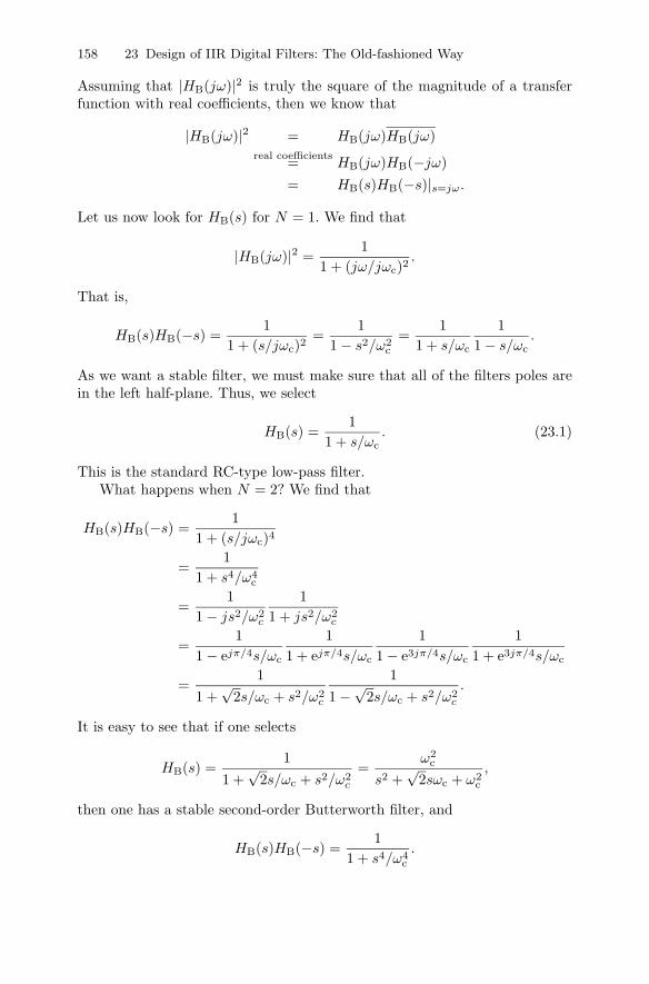
158 23 Design of IIR Digital Filters: The Old-fashioned Way
Assuming that |HB(jω)|2 is truly the square of the magnitude of a transferfunction with real coefficients, then we know that
|HB(jω)|2 = HB(jω)HB(jω)real coefficients= HB(jω)HB(−jω)
= HB(s)HB(−s)|s=jω.
Let us now look for HB(s) for N = 1. We find that
|HB(jω)|2 =1
1 + (jω/jωc)2.
That is,
HB(s)HB(−s) =1
1 + (s/jωc)2=
11 − s2/ω2
c
=1
1 + s/ωc
11 − s/ωc
.
As we want a stable filter, we must make sure that all of the filters poles arein the left half-plane. Thus, we select
HB(s) =1
1 + s/ωc. (23.1)
This is the standard RC-type low-pass filter.What happens when N = 2? We find that
HB(s)HB(−s) =1
1 + (s/jωc)4
=1
1 + s4/ω4c
=1
1 − js2/ω2c
11 + js2/ω2
c
=1
1 − ejπ/4s/ωc
11 + ejπ/4s/ωc
11 − e3jπ/4s/ωc
11 + e3jπ/4s/ωc
=1
1 +√
2s/ωc + s2/ω2c
11 −√
2s/ωc + s2/ω2c
.
It is easy to see that if one selects
HB(s) =1
1 +√
2s/ωc + s2/ω2c
=ω2
c
s2 +√
2sωc + ω2c
,
then one has a stable second-order Butterworth filter, and
HB(s)HB(−s) =1
1 + s4/ω4c
.
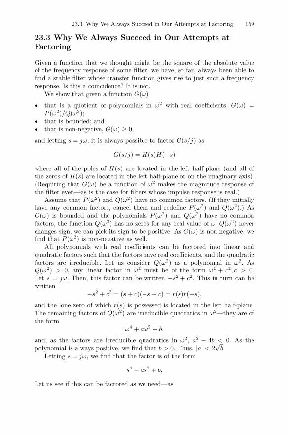
23.3 Why We Always Succeed in Our Attempts at Factoring 159
23.3 Why We Always Succeed in Our Attempts atFactoring
Given a function that we thought might be the square of the absolute valueof the frequency response of some filter, we have, so far, always been able tofind a stable filter whose transfer function gives rise to just such a frequencyresponse. Is this a coincidence? It is not.
We show that given a function G(ω)
• that is a quotient of polynomials in ω2 with real coefficients, G(ω) =P (ω2)/Q(ω2);
• that is bounded; and• that is non-negative, G(ω) ≥ 0,
and letting s = jω, it is always possible to factor G(s/j) as
G(s/j) = H(s)H(−s)
where all of the poles of H(s) are located in the left half-plane (and all ofthe zeros of H(s) are located in the left half-plane or on the imaginary axis).(Requiring that G(ω) be a function of ω2 makes the magnitude response ofthe filter even—as is the case for filters whose impulse response is real.)
Assume that P (ω2) and Q(ω2) have no common factors. (If they initiallyhave any common factors, cancel them and redefine P (ω2) and Q(ω2).) AsG(ω) is bounded and the polynomials P (ω2) and Q(ω2) have no commonfactors, the function Q(ω2) has no zeros for any real value of ω. Q(ω2) neverchanges sign; we can pick its sign to be positive. As G(ω) is non-negative, wefind that P (ω2) is non-negative as well.
All polynomials with real coefficients can be factored into linear andquadratic factors such that the factors have real coefficients, and the quadraticfactors are irreducible. Let us consider Q(ω2) as a polynomial in ω2. AsQ(ω2) > 0, any linear factor in ω2 must be of the form ω2 + c2, c > 0.Let s = jω. Then, this factor can be written −s2 + c2. This in turn can bewritten
−s2 + c2 = (s + c)(−s + c) = r(s)r(−s),
and the lone zero of which r(s) is possessed is located in the left half-plane.The remaining factors of Q(ω2) are irreducible quadratics in ω2—they are ofthe form
ω4 + aω2 + b,
and, as the factors are irreducible quadratics in ω2, a2 − 4b < 0. As thepolynomial is always positive, we find that b > 0. Thus, |a| < 2
√b.
Letting s = jω, we find that the factor is of the form
s4 − as2 + b.
Let us see if this can be factored as we need—as
160 23 Design of IIR Digital Filters: The Old-fashioned Way
r(s)r(−s) = (s2 + αs + β)((−s)2α(−s) + β)
where the first factor, r(s), has no zeros in the right half-plane. The productabove is equal to
s4 + (2β − α2)s2 + β2.
Equating coefficients with our original fourth-order polynomial, we find thatβ2 = b and 2β − α2 = a. As we would like r(s) to have all of its zeros in theright half-plane, the polynomial’s coefficients must all have the same sign [6].Thus, we let β = +
√b. We find that 2
√b − α2 = −a. That is, α2 = 2
√b + a.
As we have shown that 2√
b + a > 0, the square root is real, and we find thatα =
√2√
b + a. We have shown that each factor of Q(ω2) can be factored inprecisely the fashion that we need.
P (ω2) is a little harder to handle, because in addition to having terms ofthe types Q(ω2) has, it can have zeros. Because P (ω2) cannot change sign, anyzeros of the form ω2 − c, c > 0 must have even multiplicity. Let us considera single such double zero in ω2, (ω2 − c)2. Let us see if our new polynomialcan be factored as needed. Letting s = jω, we find that we must consider(s2 + c)2. Noting that
(s2 + c)2 = r(s)r(−s) ≡ (s2 + c)((−s)2 + c),
we find that the new type of factor can itself be factored. The last possibletype of zero is the polynomial ω2 itself. As this function is non-negative, itneed not appear with even multiplicity. Letting ω = s/j, we find that
−s2 = r(s)r(−s) = s(−s).
Here, too, we have succeeded in factoring the term of interest.We have shown that given a function G(ω) that satisfies the list of prop-
erties above, one can always find a function H(s) such that
H(s)H(−s) = G(s/j).
As the polynomials that make up the denominator of H(s) have all of theirroots in the left half-plane, the function H(s) corresponds to a stable system.Additionally, the polynomials that make up the numerator can be chosen insuch a way that all of their roots lie in the left half-plane or on the imaginaryaxis.
23.4 The Bilinear Transform
We have described several types of analog filters, and we have seen how todesign Nth-order continuous-time Butterworth and Chebyshev filters. Howcan we take this knowledge and, without needing to think too much, convertit into knowledge about a digital filter?
23.5 The Passage from Analog Filter to Digital Filter 161
We use the bilinear transform. The bilinear transform, which we developmomentarily, can be used to transform the transfer function of a stable analogfilter into the transfer function of a similar stable digital filter.
The bilinear transform is defined by
z = B(s) ≡ 1 + (T/2)s1 − (T/2)s
.
Its inverse iss = B−1(z) =
2T
z − 1z + 1
.
This mapping is (essentially) a one-to-one and onto mapping of the complexplane into itself in such a way that B(s) maps the imaginary axis onto theunit circle, the left half-plane into the interior of the unit circle and the righthalf-plane into the exterior of the unit circle [6]. One might say that it takesstable causal filters into stable causal filters. It is also easy to see that thebilinear transform takes Nth-order filters into Nth-order filters.
To see how the bilinear transform maps the unit circle, consider s = B−1(z)for z = eTj2πf . We find that
B−1(z) =2T
eTj2πf − 1eTj2πf + 1
=2T
j tan(T2πf/2).
When Tf is small, this is approximately j2πf—which is the correct frequencyin the “continuous-time domain.”
Consider a continuous-time filter whose transfer function is H(s) andwhose frequency response is H(jω). Making use of the bilinear transform toconvert this filter into a discrete-time filter, we find that the transfer functionof the discrete-time filter is given by H(B−1(z)), and its frequency responseis given by
H(B−1(ej2πfT )) = H(2j tan(Tπf)/T ).
Because when θ is small, tan(θ) ≈ θ, we find that as long as Tf is small,
H(B−1(ej2πfT )) ≈ H(2jπf) = H(jω).
That is, as long as f is small relative to the sampling frequency, the frequencyresponse of the discrete-time filter is approximately the same as that of thecontinuous-time filter from which it was derived. (See Exercise 3 for informa-tion about prewarping—which is a way of dealing with the non-linearity inthe mapping from the unit circle to the imaginary axis.)
23.5 The Passage from Analog Filter to Digital Filter
Let us consider the simple RC-type filter of (23.1)—the first-order Butter-worth filter—and transform it into a digital filter. We replace every s withB−1(z). We find that
162 23 Design of IIR Digital Filters: The Old-fashioned Way
T (z) =1
1 + B−1(z)/ωc=
Tωc(z + 1)Tωc(z + 1) + 2(z − 1)
.
The pole of this filter is located at
z =2 − Tωc
2 + Tωc.
If T is small enough, then this number is positive and less than one. When Tis large, the pole is negative and less than one in absolute value. Additionally,T (z = 1) = 1—the system passes DC signals without change.
23.6 MATLAB and the Bilinear Transform
MATLAB r© has a command, c2d, whose purpose is to convert continuous-time filters to discrete-time filters. The command has many options—as thereare many ways of converting continuous-time filters to discrete-time filters.
Suppose that one would like to take a second-order, low-pass Butterworthfilter whose cut-off frequency is 100 Hz, and convert it into a digital filter whosesampling rate is 1 kHz. On p. 158 we designed a second-order Butterworth fil-ter. The program of Figure 23.2 defines the continuous-time transfer function,H, and then uses c2d to convert the filter to a discrete-time filter. Note thatwhen used without a sample time, the command tf produces a continuous-time transfer function object (and MATLAB uses s to represent the transferfunction’s variable). The format of the c2d command, when used to convert acontinuous-time transfer function object to a discrete-time transfer functionobject, is
c2d(continuous-time transfer function, sample time, ’tustin’).
The third element of the command, the string ’tustin’, tells MATLAB to makethe conversion using the bilinear transform2, rather than one of the othermethods for converting continuous-time transfer functions to discrete-timetransfer functions. The command hold on causes MATLAB to plot figures onthe same set of axes. This makes it easy to use MATLAB to compare plots.Additionally, the command legend causes MATLAB to produce a legend fora figure.
The figure output by the sequence of commands given in Figure 23.2 ispresented in Figure 23.3. Note that the frequency responses are substantiallyidentical at low frequencies, but as the Nyquist frequency is approached thefilters behave differently. This is precisely what we should have expected. Atlow frequencies the frequency response of the continuous-time filter is mappedinto that of the discrete-time filter almost without change. As the frequencyincreases, the mapping starts to warp the response. That is why the responsesdiffer at high frequencies.2 Arnold Tustin (1899–1994) introduced the bilinear transform that bears his name
to the control community to relate discrete-time and continuous-time systems [2].
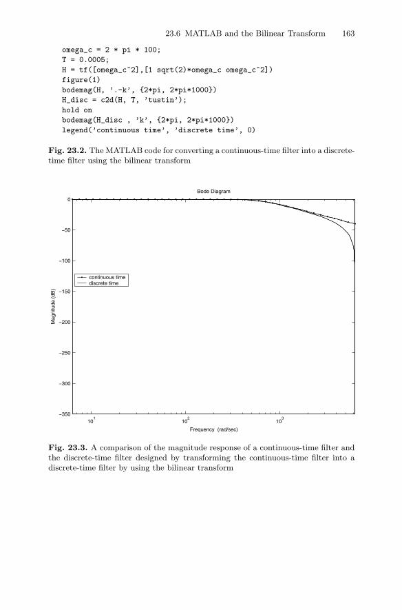
23.6 MATLAB and the Bilinear Transform 163
omega_c = 2 * pi * 100;
T = 0.0005;
H = tf([omega_c^2],[1 sqrt(2)*omega_c omega_c^2])
figure(1)
bodemag(H, ’.-k’, {2*pi, 2*pi*1000})
H_disc = c2d(H, T, ’tustin’);
hold on
bodemag(H_disc , ’k’, {2*pi, 2*pi*1000})
legend(’continuous time’, ’discrete time’, 0)
Fig. 23.2. The MATLAB code for converting a continuous-time filter into a discrete-time filter using the bilinear transform
101
102
103
−350
−300
−250
−200
−150
−100
−50
0
Mag
nitu
de (
dB)
continuous timediscrete time
Bode Diagram
Frequency (rad/sec)
Fig. 23.3. A comparison of the magnitude response of a continuous-time filter andthe discrete-time filter designed by transforming the continuous-time filter into adiscrete-time filter by using the bilinear transform
164 23 Design of IIR Digital Filters: The Old-fashioned Way
23.7 The Experiment
Design a third-order analog Butterworth filter whose cut-off frequency is135 Hz. Use the bilinear transform to convert the analog design into a digitalone. Let Ts = 1/1,350 s. In the laboratory report, show all the computations.MATLAB may be used to help with the computations, but its built-in filter-design tools may not be used to help with the design. Implement the filteryou design in C, and demonstrate that the filter works as predicted.
23.8 Exercises
1. Show thatdn
dωn|HB(jω)|2
∣∣∣∣ω=0
= 0, n = 1, . . . , 2N − 1.
2. Show that when the pole of the filter in Section 23.5 is negative, the stepresponse of the digital filter is not monotonic even though the filter isfirst-order. Could this happen to the stable analog filter from which thedigital filter was designed?
3. What is prewarping? When should one make use of this technique?4. Derive the identity
cos((N + 1)θ) = 2 cos(θ) cos(Nθ) − cos((N − 1)θ).
You may find this problem easier if you “rephrase” the identity as
cos((N + 1)θ) + cos((N − 1)θ) = 2 cos(θ) cos(Nθ).
5. Show that for x outside the interval [−1, 1], the function |VN (x)| increasesmonotonically. You may wish to proceed as follows:a) Note that because VN (x) has N distinct zeros in the region [−1, 1],
the function V ′N (x) must have N − 1 zeros in that region. In fact, the
N −1 zeros must be sandwiched between the N zeros of VN (x). (Thisis a simple consequence of Rolle’s theorem [17].)
b) As V ′N (x) is an N − 1th-order polynomial, these N − 1 zeros are all of
the zeros of V ′N (x).
c) We find that the value of the derivative of VN (x) is of one sign to theleft of the first zero and is of one sign to the right of the last zero.This allows us to finish the proof.
6. a) Calculate HC(s) for N = 2, ε = 1, and ωc = 1.b) Make use of the bilinear transform to produce a second-order digital
Chebyshev filter from the filter of the previous section. Let Ts = 10ms.c) Examine the magnitude responses of the filters of the previous sections
by making use of the MATLAB bodemag command. Compare theresponses of the discrete-time and continuous-time systems.
7. Show that when Tωc = 2, the filter of Section 23.5 is an FIR low-passfilter.
24
New Filters from Old
Summary. In Chapter 23, we saw how to design low-pass digital filters using low-pass analog filters as a starting point. In this chapter, we describe one way of takingdigital low-pass filters and converting them into other types of digital filters bytransforming the filters’ transfer functions according to simple rules.
Keywords. filter transformations, Blaschke products.
24.1 Transforming Filters
Let H(z) be the transfer function of a stable filter, and let G(z) be a functionthat
• is analytic for |z| ≤ 1, and• satisfies |G(z)| = 1 when |z| = 1.
What can be said about H(G(z))? As G(z) maps points on the unit circle backto the unit circle, we can say that G(z) “reorganizes” the frequency responseof the filter. Functions like G(z)—which map the unit circle into itself—mightpossibly help us reorganize the frequency response of a low-pass filter intothat of another type of filter.
24.2 Functions that Take the Unit Circle into Itself
It is easy to show that the absolute value of an analytic function, G(z), ina domain is less than or equal to the absolute value of the function on theboundary of the domain—and this shows that if G(z) takes the unit circle intoitself, then inside the unit disk, |G(z)| ≤ 1. The maximum modulus principle[3, p. 136] asserts that if the absolute value of an analytic function achievesits maximum inside a “reasonable domain,” then the function is a constant
166 24 New Filters from Old
within the domain. Given an analytic function f(z) with no zeros inside agiven domain, and considering the function 1/f(z), one can show that theminimum of the absolute value of the function in a “reasonable domain” mustbe greater than or equal to the minimum value of the absolute value on theboundary.
Let us consider a generic function, G(z), that is analytic in the closed unitdisk, |z| ≤ 1, and that maps the unit circle into the unit circle. Because G(z)maps the unit circle into the unit circle, we find that |G(ejθ)| = 1. Thus, wefind that inside the unit disk, |G(z)| ≤ 1. If in addition G(z) has no zeros inthe unit disk, then we find that inside the unit disk |G(z)| ≥ 1. This showsthat if G(z) has no zeros inside the unit disk, then |G(z)| = 1 throughout theunit disk. The maximum modulus principle then asserts that G(z) = c. Inlight of the fact that |G(z)| = 1, we find that G(z) = ejθ (where 0 ≤ θ < 2π).
This fact can be used to characterize all functions that are analytic insidethe unit disk and that map the unit circle into itself. Let us consider a functionof this sort, G(z), that has a single zero of multiplicity one inside the unit diskat the point z0. Consider the function
f(z) = G(z)1 − z0z
z0 − z.
Clearly, f(z) has no zeros inside the unit disk—we have removed the only zeroit had. The zero we have added is located at z = 1/z0, and |z| > 1. Let usconsider how f(z) maps the unit circle.
When z = ejθ, the second part of f(z) satisfies
1 − z0ejθ
z0 − ejθ=
1ejθ
1 − z0ejθ
z0e−jθ − 1
=1
ejθ
1 − c
c − 1, c = z0ejθ.
The absolute value of this expression is always one. Thus, the function f(z)is analytic, maps the unit circle into the unit circle, and has no zeros insidethe unit disk. We conclude that f(z) = ejθ (where θ is in no way related tothe θ in the proof). We find that (at least inside and on the unit disk)
G(z) = ejθ z0 − z
1 − z0z.
As we know that |G(z)| = 1 on the unit circle, we know that |G(z)| ≤ 1in the closed unit disk—that G(z) maps the unit disk into the unit disk. Itis easy to show that G(z) is a one-to-one and onto mapping of the complexplane into itself. (See Exercise 5.) As we know that G(z) maps the unit circleinto itself, maps the unit disk into itself, and that G(z) is continuous, it iseasy to show that G(z) must also map the exterior of the unit disk into theexterior of the unit disk.
24.3 Converting a Low-pass Filter into a High-pass Filter 167
The same trick that we used to remove a single zero can be used to removeas many zeros as the function has. Thus, all functions that are analytic insideand on the unit disk, that have a finite number of zeros inside the unit disk,and that map the unit circle into itself must be of the form
ejθN∏
k=1
zk − z
1 − zkz, |zk| < 1. (24.1)
(Such functions are known as finite Blaschke products [18].) It is easy to seethat such functions map the exterior of the unit disk to the exterior of theunit disk.
Let G(z) be such a function, let H(z) be the transfer function of a stablefilter, and consider H(G(z)). Since G(z) maps the exterior of the unit diskinto itself, if |z| > 1, then |G(z)| > 1. As H(z) corresponds to a stable filter,it has no poles outside the unit disk. Thus, H(G(z)) cannot be infinite if zis outside the unit disk. We find that H(G(z)) has no poles outside the unitdisk and is, consequently, the transfer function of a stable filter. Because G(z)is a rational function of z, H(G(z)) is as well. As G(z) takes points on theunit circle to points on the unit circle, the frequency response of the filterwhose transfer function is given by H(G(z)) is a “rearranged” version of thefrequency response of the original filter.
In the following sections, we make use of finite Blaschke products to re-arrange the frequency response of a digital filter so that it becomes a differenttype of digital filter. (A more complete set of filter transformation rules canbe found in [4].)
24.3 Converting a Low-pass Filter into a High-pass Filter
The first of the mappings—of the reorganizations—that we consider is themapping for which N = 1, z1 = 0, and ejθ = +1. That is, we consider themapping −z. It is easy to see that under this mapping, low frequencies—which correspond to values of z near 1—go over to high frequencies—whichcorrespond to values of z near −1.
Consider the simple low-pass filter
Glp(z) = (1 − α)z
z − α, 0 < α < 1.
Under our mapping, this becomes
Ghp(z) = (1 − α)z
z + α, 0 < α < 1.
It is easy to show that this is indeed a high-pass filter. Using MATLAB r© andits bodemag command, it is even easier to see that this is a high-pass filter.
Consider, for example, the filter for which α = 1/2 and Ts = 1ms. GivingMATLAB the commands
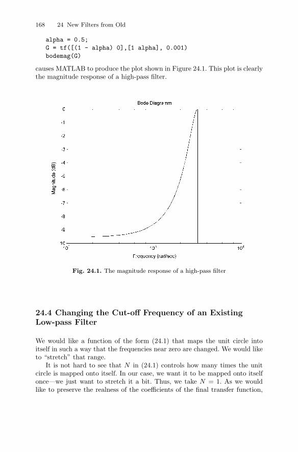
168 24 New Filters from Old
alpha = 0.5;G = tf([(1 - alpha) 0],[1 alpha], 0.001)bodemag(G)
causes MATLAB to produce the plot shown in Figure 24.1. This plot is clearlythe magnitude response of a high-pass filter.
Fig. 24.1. The magnitude response of a high-pass filter
24.4 Changing the Cut-off Frequency of an ExistingLow-pass Filter
We would like a function of the form (24.1) that maps the unit circle intoitself in such a way that the frequencies near zero are changed. We would liketo “stretch” that range.
It is not hard to see that N in (24.1) controls how many times the unitcircle is mapped onto itself. In our case, we want it to be mapped onto itselfonce—we just want to stretch it a bit. Thus, we take N = 1. As we wouldlike to preserve the realness of the coefficients of the final transfer function,
24.4 Changing the Cut-off Frequency of an Existing Low-pass Filter 169
we require that ejθ = ±1 and z1 ∈ R. As |z1| < 1, this leaves us with the setof mappings
Tz1(z) ≡ ± z1 − z
1 − z1z, −1 < z1 < 1.
Note that T (1) = ±(−1). If we are looking to take low-pass filters into low-pass filters, we must limit ourselves to filters of the form
Tz1(z) ≡ − z1 − z
1 − z1z=
z − z1
1 − z1z.
Such filters will change the cut-off frequency of a low-pass filter. To obtain ahigh-pass filter with a specific cut-off frequency, one would compose the twomappings −z and Tz1(z); one would make use of the mapping −Tz1(z).
Let us consider the action of the mappings
Ta(z) =z − a
1 − az, −1 < a < 1
in greater detail. We find that this mapping takes the point z = e2πjfTs tothe point
Ta(e2πjfTs) = e2πjfTs1 − ae−2πjfTs
1 − ae2πjfTs= e2πjfTs
1 − ae−2πjfTs
(1 − ae−2πjfTs
) .
We know that our mappings take the unit circle into the unit circle. Thus,the magnitude of this point must be one. The phase of the point is
� Ta(e2πjfTs) = 2πfTs + 2 tan−1
(a sin(2πfTs)
1 − a cos(2πfTs)
).
We find that the mapping shifts lower frequencies to higher ones if a is positive,and it shifts higher frequencies to lower ones if a is negative.
Let us consider an example. Suppose that we have a low-pass filter thatpasses frequencies up to 1 Hz, and we would like a low-pass filter that passesfrequencies up to 10 Hz. We can make use of our transformation to design afunction that will transform our filter appropriately.
We are looking for an a for which an input of 10 Hz is converted into theangle that is appropriate to 1 Hz. Thus, we must solve the equation
2π1Ts = 2π10Ts + 2 tan−1
(a sin(2π10Ts)
1 − a cos(2π10Ts)
).
Let us take Ts = 1ms—let us consider a filter that samples 1,000 times persecond. We find that we are now looking for the solution of the equation
tan(−0.001 × 9π) =a sin(2π0.01)
1 − a cos(2π0.01).
170 24 New Filters from Old
Solving for a, we find thata = −0.8182.
Thus, the mapping
Ta(z) =z + 0.81821 + 0.8182z
can be used to convert a low-pass filter that takes 1,000 samples per sec-ond, and whose cut-off frequency is 1 Hz, into a low-pass filter whose cut-offfrequency is 10 Hz.
24.5 Going from a Low-pass Filter to a Bandpass Filter
We have seen that the transforms Tz1(z),−1 < z1 < 1, take low-pass filtersinto other low-pass filters by traversing the unit circle at different “rates.”If one takes two such transforms and multiplies them, one causes the unitcircle to be traversed once as f goes from zero to 1/(2Ts). Such a transfor-mation causes the low-pass filter to become a bandstop filter. If one uses thetransformation on a high-pass filter, the high-pass filter becomes a bandpassfilter.
Suppose that TLP(z) is the transfer function of a low-pass filter. We havefound that TLP(−Tα(z)Tβ(z)) is a bandpass filter. Suppose that TLP(z) is alow-pass filter with cut-off frequency Fc, and that we let α = β = 0—wechoose Tα(z) = Tβ(z) = z. Let us characterize the filter given by
T (z) = TLP(−z2).
Substituting z = e2πjfTs in T (z), we find that
T (e2πjfTs) = TLP(−e4πjfTs) = TLP(ej2π(2f−Fs/2)Ts).
When f = 0, the frequency response of T (z) corresponds to the response ofthe low-pass filter when f = −Fs/2. This will be very small—as seen in Figure24.2. (Figure 24.2 is the magnitude response of a typical low-pass filter. In thesample system, Fs = 100Hz, and we have plotted the magnitude responsefrom −1/(2Ts) to 1/(2Ts).) As f increases, the magnitude of the frequencyresponse increases. When f = Fs/4 − Fc/2, the frequency response of thenew filter corresponds to that of the low-pass filter at the (left-hand) cut-offfrequency. When f reaches f = Fs/4, the response corresponds to that ofthe low-pass filter at f = 0. As f increases further, the response of the filterstarts to “fall off.” At f = Ts/4 + Fc/2, the filter has once again reached thelow-pass filter’s cut-off frequency. When f = 1/(2Ts), the response of the newfilter corresponds to that of the low-pass filter at f = Fs/2—and should, onceagain, be very small. We find that the new filter is a (symmetric) bandpassfilter, and its cut-off frequencies are Fs/4 − Fc/2 and Fs/4 + Fc/2.
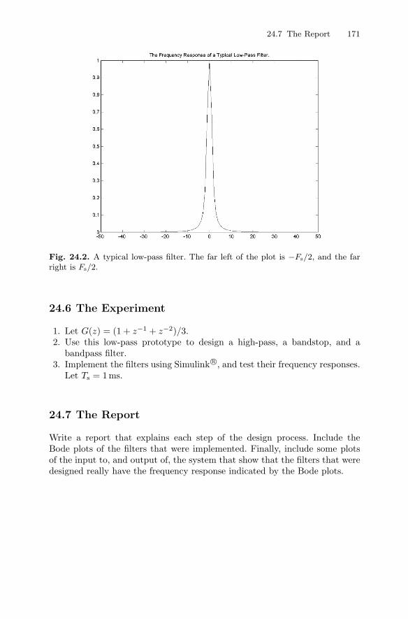
24.7 The Report 171
Fig. 24.2. A typical low-pass filter. The far left of the plot is −Fs/2, and the farright is Fs/2.
24.6 The Experiment
1. Let G(z) = (1 + z−1 + z−2)/3.2. Use this low-pass prototype to design a high-pass, a bandstop, and a
bandpass filter.3. Implement the filters using Simulink r©, and test their frequency responses.
Let Ts = 1ms.
24.7 The Report
Write a report that explains each step of the design process. Include theBode plots of the filters that were implemented. Finally, include some plotsof the input to, and output of, the system that show that the filters that weredesigned really have the frequency response indicated by the Bode plots.
172 24 New Filters from Old
24.8 Exercises
1. Show that the functions of (24.1) define unstable all-pass.2. Show that if one replaces z of (24.1) by z−1, then the functions represent
stable all-pass filters.3. Consider the analog prototype low-pass filter
G(s) =1
s + 1.
a) Using the bilinear transform, convert this into a digital low-pass filter.(The resulting transfer function will depend on the sampling rate.)
b) Let Ts = 100μs. Using the low-pass to bandpass transformation z →−z2, convert the low-pass digital filter into a bandpass digital filter.
c) Use MATLAB to plot the filter’s Bode plots.4. Design a third-order high-pass Butterworth filter. Let Ts = 100μs, and let
the cut-off frequency of the filter be 4 kHz. Check that your filter meetsthe specifications by using MATLAB. You will probably want to designthe filter bya) Designing a continuous-time low-pass Butterworth filter with a cut-off
frequency of 1 Hz.b) Modifying the filter to have a cut-off frequency that will lead to a
final design with a cut-off frequency of 4 kHz. (How does one find thecut-off frequency of the low-pass filter?)
c) Converting the continuous-time filter into a discrete-time filter bymaking use of the bilinear transform.
d) Converting the low-pass filter into a high-pass filter.5. Show that the function
K(z) =zk − z
1 − zzk
satisfies the equation K(K(z)) = z. Explain how this shows that thefunction K(z) is a one-to-one and onto mapping of the complex planeinto itself. As G(z) = ejθK(z), conclude that G(z) is also a one-to-oneand onto mapping of the complex plane into itself.
25
Implementing an IIR Digital Filter
Summary. We now understand how to “design” a recurrence relation that imple-ments a digital filter. In this chapter, we consider how such equations should beimplemented. We discuss several methods of implementing digital filters, and wefind that due to numerical stability issues, it is best to implement high-order filtersby using biquads.
Keywords. direct form I realization, direct form II realization, numerical stability,
biquads.
25.1 Introduction
As the digital filters that are of interest to us can be described by transferfunctions that are rational functions of z−1, it is easy to show that the filterscan be described by equations of the form
yn =M∑
m=1
bmyn−m +L∑
l=0
alxn−l. (25.1)
Translating this into a transfer function, we find that the transfer function ofa system described by (25.1) is
T (z) =Y (z)X(z)
=∑L
l=0 alz−1
1 −∑Mm=1 bmz−m
.
There are many possible ways that one can actually calculate the sums of(25.1). The simplest is to perform the calculations as given—in one fell swoop.We consider this method in Section 25.2. In later sections, we examine moreinteresting and effective techniques.
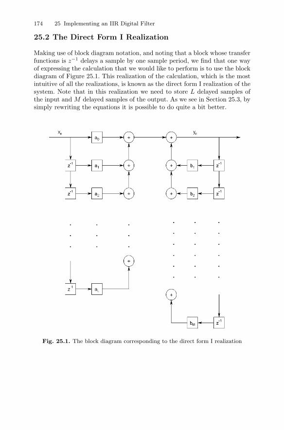
174 25 Implementing an IIR Digital Filter
25.2 The Direct Form I Realization
Making use of block diagram notation, and noting that a block whose transferfunctions is z−1 delays a sample by one sample period, we find that one wayof expressing the calculation that we would like to perform is to use the blockdiagram of Figure 25.1. This realization of the calculation, which is the mostintuitive of all the realizations, is known as the direct form I realization of thesystem. Note that in this realization we need to store L delayed samples ofthe input and M delayed samples of the output. As we see in Section 25.3, bysimply rewriting the equations it is possible to do quite a bit better.
Fig. 25.1. The block diagram corresponding to the direct form I realization
25.4 Trouble in Paradise 175
25.3 The Direct Form II Realization
By reconsidering the transfer function, it is possible to substantially reducethe number of samples that need to be stored. Let us define the auxiliaryvariable wn by the equation
W (z) =1
1 −∑Mm=1 bmz−m
X(z),
and note that with this definition we find that Y (z) satisfies
Y (z) =L∑
l=0
alz−lW (z).
Both wn and yn depend on previous values of wn but not on previous valuesof either yn or xn. The block diagram of a wn-based system is given in Figure25.2. We find that the number of delays necessary here—and the number ofelements that must be stored here—is the larger of L and M . If these numbersare roughly equal, then this method reduces the number of terms that must bestored by nearly half. This realization of the calculation is known as the directform II realization. In Figure 25.2, the last of the al is given as aM , rather thanas aL. This is done because generally L ≤ M—because the transfer functionis generally proper. If L < M , we let
al = 0, l = L + 1, . . . M.
In this way, the figure correctly and simply represents the calculations thatwe need to perform.
25.4 Trouble in Paradise
It turns out that both of the realizations we have seen so far are problem-atic when M or L is even reasonably large. What is the problem? Generallyspeaking, the coefficients of the polynomials in the transfer function are im-plemented in some type of finite precision arithmetic. That means that thecoefficients used in the actual calculations are not precisely the coefficientsthat were planned. Perturbing the coefficients of a polynomial perturbs thelocation of the polynomial’s roots. The roots of the denominator are the polesof the system, and if the poles leave the unit disk, then the system becomesunstable.
Let us see how perturbing the coefficients of a polynomial affects the place-ment of the roots of the polynomial. Consider a polynomial of the form
P (z) = 1 −M∑
m=1
bmz−m.
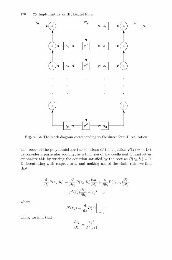
176 25 Implementing an IIR Digital Filter
Fig. 25.2. The block diagram corresponding to the direct form II realization
The roots of the polynomial are the solutions of the equation P (z) = 0. Letus consider a particular root, zk, as a function of the coefficient bi, and let usemphasize this by writing the equation satisfied by the root as P (zk, bi) = 0.Differentiating with respect to bi and making use of the chain rule, we findthat
ddbi
P (zk, bi) =∂
∂zkP (zk, bi)
∂zk
∂bi+
∂
∂biP (zk, bi)
∂bi
∂bi
= P ′(zk)∂zk
∂bi− z−i
k = 0
where
P ′(zk) =ddz
P (z)∣∣∣∣z=zk
.
Thus, we find that∂zk
∂bi=
z−ik
P ′(zk).
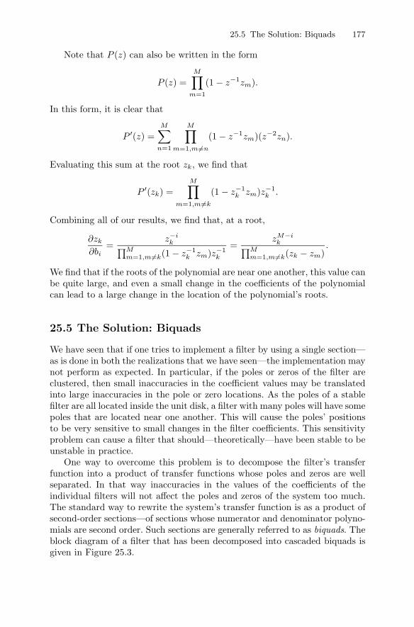
25.5 The Solution: Biquads 177
Note that P (z) can also be written in the form
P (z) =M∏
m=1
(1 − z−1zm).
In this form, it is clear that
P ′(z) =M∑
n=1
M∏
m=1,m �=n
(1 − z−1zm)(z−2zn).
Evaluating this sum at the root zk, we find that
P ′(zk) =M∏
m=1,m �=k
(1 − z−1k zm)z−1
k .
Combining all of our results, we find that, at a root,
∂zk
∂bi=
z−ik∏M
m=1,m �=k(1 − z−1k zm)z−1
k
=zM−i
k∏Mm=1,m �=k(zk − zm)
.
We find that if the roots of the polynomial are near one another, this value canbe quite large, and even a small change in the coefficients of the polynomialcan lead to a large change in the location of the polynomial’s roots.
25.5 The Solution: Biquads
We have seen that if one tries to implement a filter by using a single section—as is done in both the realizations that we have seen—the implementation maynot perform as expected. In particular, if the poles or zeros of the filter areclustered, then small inaccuracies in the coefficient values may be translatedinto large inaccuracies in the pole or zero locations. As the poles of a stablefilter are all located inside the unit disk, a filter with many poles will have somepoles that are located near one another. This will cause the poles’ positionsto be very sensitive to small changes in the filter coefficients. This sensitivityproblem can cause a filter that should—theoretically—have been stable to beunstable in practice.
One way to overcome this problem is to decompose the filter’s transferfunction into a product of transfer functions whose poles and zeros are wellseparated. In that way inaccuracies in the values of the coefficients of theindividual filters will not affect the poles and zeros of the system too much.The standard way to rewrite the system’s transfer function is as a product ofsecond-order sections—of sections whose numerator and denominator polyno-mials are second order. Such sections are generally referred to as biquads. Theblock diagram of a filter that has been decomposed into cascaded biquads isgiven in Figure 25.3.
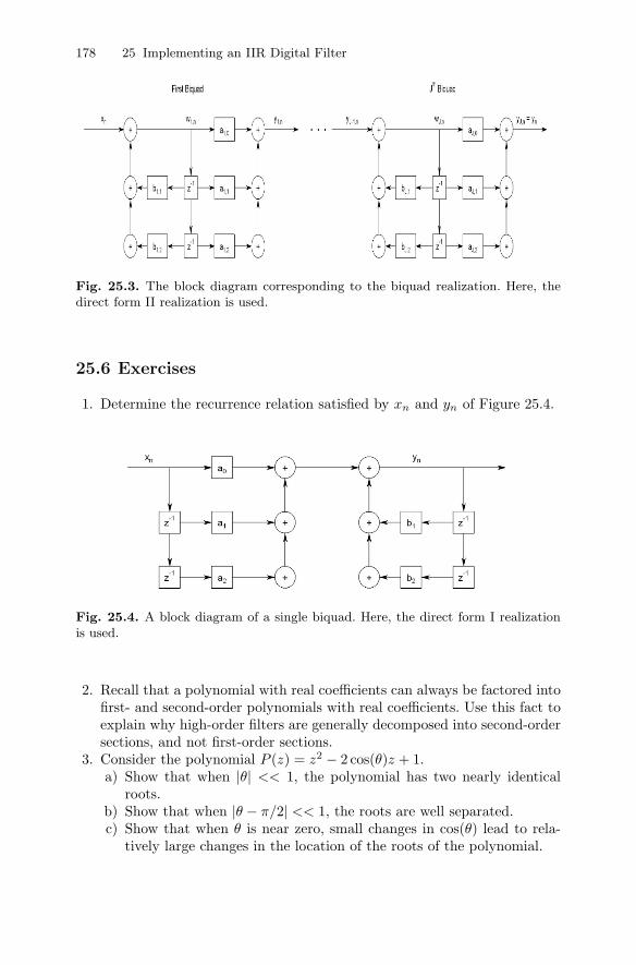
178 25 Implementing an IIR Digital Filter
Fig. 25.3. The block diagram corresponding to the biquad realization. Here, thedirect form II realization is used.
25.6 Exercises
1. Determine the recurrence relation satisfied by xn and yn of Figure 25.4.
Fig. 25.4. A block diagram of a single biquad. Here, the direct form I realizationis used.
2. Recall that a polynomial with real coefficients can always be factored intofirst- and second-order polynomials with real coefficients. Use this fact toexplain why high-order filters are generally decomposed into second-ordersections, and not first-order sections.
3. Consider the polynomial P (z) = z2 − 2 cos(θ)z + 1.a) Show that when |θ| << 1, the polynomial has two nearly identical
roots.b) Show that when |θ − π/2| << 1, the roots are well separated.c) Show that when θ is near zero, small changes in cos(θ) lead to rela-
tively large changes in the location of the roots of the polynomial.
25.6 Exercises 179
d) Finally, show that when θ is near π/2, small changes in cos(θ) do notaffect the location of the roots as much as they did in the previouscase.
4. a) Design a fourth-order continuous-time Butterworth low-pass filterwith a cut-off frequency of ωc = 10 rad s−1.
b) Using the bilinear transform, transform this filter into a digital filterfor which Ts = 0.001 s.
c) Find the recurrence relation satisfied by the filter’s input and output.d) Give a schematic drawing (with all the filter coefficients) of the filter
implemented as a cascade of two biquads realized using the direct formII realization.

26
IIR Filter Design Using MATLAB
Summary. Though it is possible to use the beautiful and interesting methods ofdays gone by to design analog or IIR digital filters, it is not strictly necessary.MATLAB r© has two different “levels” of filter-design tools. It has “regular” com-mands for filter design, and it has a graphical user interface (GUI) based filter-designtool as well. We discuss both options in the following sections.
Keywords. MATLAB, butter, fdatool.
26.1 Individual Commands
MATLAB’s suite of filter-design commands includes commands to design But-terworth, Chebyshev, and elliptic filters. As is generally the case when usingMATLAB, one can find out how things work by using the MATLAB helpcommand.
We consider the simplest command—butter. To design an Nth-order dig-ital filter with cut-off frequency ωn, one writes [b a] = butter(N, Wn). Thearrays b and a are the coefficients of the polynomials in the filter’s numeratorand denominator, respectively.
When designing a digital filter, all frequencies can be considered asbeing relative to the sampling frequency. That is, if one is sampling at100 samples s−1 and one’s cut-off frequency is 10 Hz, one can intelligently saythat one’s cut-off frequency is one-tenth the sampling frequency. In fact, ifone “speeds up” the sampling rate to 1,000 samples s−1 and one uses the samefilter—a filter that uses the same formula in its implementation—the cut-offfrequency will now be one-tenth of the new sampling rate. That is, the cut-offfrequency will be 100 Hz. (See Exercise 2.)
When using the butter command, the frequency is given relative to theNyquist frequency—relative to half the sampling frequency. The number Wnmust be between 0 and 1. The cut-off frequency will be Wn times the Nyquistfrequency of the filter that is being implemented.
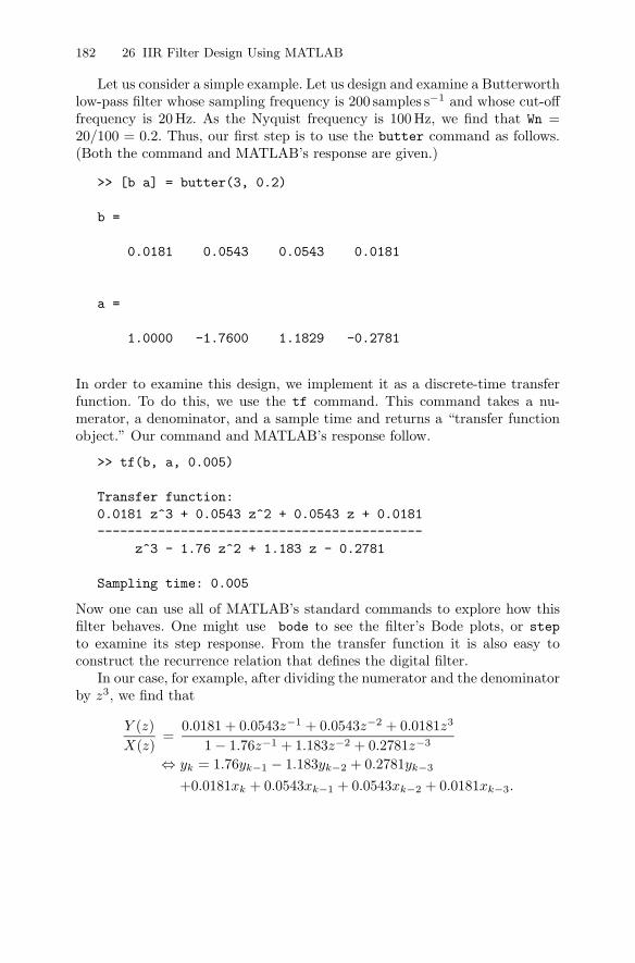
182 26 IIR Filter Design Using MATLAB
Let us consider a simple example. Let us design and examine a Butterworthlow-pass filter whose sampling frequency is 200 samples s−1 and whose cut-offfrequency is 20 Hz. As the Nyquist frequency is 100 Hz, we find that Wn =20/100 = 0.2. Thus, our first step is to use the butter command as follows.(Both the command and MATLAB’s response are given.)
>> [b a] = butter(3, 0.2)
b =
0.0181 0.0543 0.0543 0.0181
a =
1.0000 -1.7600 1.1829 -0.2781
In order to examine this design, we implement it as a discrete-time transferfunction. To do this, we use the tf command. This command takes a nu-merator, a denominator, and a sample time and returns a “transfer functionobject.” Our command and MATLAB’s response follow.
>> tf(b, a, 0.005)
Transfer function:0.0181 z^3 + 0.0543 z^2 + 0.0543 z + 0.0181-------------------------------------------
z^3 - 1.76 z^2 + 1.183 z - 0.2781
Sampling time: 0.005
Now one can use all of MATLAB’s standard commands to explore how thisfilter behaves. One might use bode to see the filter’s Bode plots, or stepto examine its step response. From the transfer function it is also easy toconstruct the recurrence relation that defines the digital filter.
In our case, for example, after dividing the numerator and the denominatorby z3, we find that
Y (z)X(z)
=0.0181 + 0.0543z−1 + 0.0543z−2 + 0.0181z3
1 − 1.76z−1 + 1.183z−2 + 0.2781z−3
⇔ yk = 1.76yk−1 − 1.183yk−2 + 0.2781yk−3
+0.0181xk + 0.0543xk−1 + 0.0543xk−2 + 0.0181xk−3.
26.4 The Experiment: Part II 183
26.2 The Experiment: Part I
Use the built-in MATLAB commands to design a second-order Butterworthlow-pass filter. Design the filter to have a cut-off frequency of 270 Hz when thesampling rate is 2,700 samples s−1. Implement the filter using the ADuC841.Measure the frequency response of the filter at several frequencies and comparethe results with those predicted by the theory.
When implementing the filter, consider carefully what data type(s) to usein your C program. Make sure that, on the one hand, you have enough bitsfor your needs. On the other hand, make sure that you do not make themicroprocessor’s job too hard. Floating point arithmetic is rather hard onsimple microprocessors like the ADuC841.
26.3 Fully Automatic Filter Design
In addition to the “discrete filter-design commands,” MATLAB also providesa “filter design and analysis tool.” This tool is invoked by typing fdatool atthe MATLAB command line. This tool will design most any filter. It asks foryour specifications and returns the Bode plots of the filter it designs. Thistool has many display and implementation options. Play with it a little bit tosee what it can do!
26.4 The Experiment: Part II
Use fdatool to design a third-order low-pass elliptic filter. Let the cut-offfrequency of the filter be 270 Hz and the sampling frequency be 2,700 samplesper second. Let the passband ripple—the extent to which the magnitude isallowed to vary in the passband—be 1 dB, and make the magnitude in thestopband at least 30 dB below the passband magnitude.
Note that MATLAB uses second-order sections—biquads—in its defaultfilter implementation. For a third-order filter, one probably does not need touse this type of implementation. To change the implementation type, right-click on the “Current Filter Information” box, and click on “convert to singlesection.” In order to see the filter coefficients, either click on the button labeled“[b/a]” in the toolbar or go to the File tab, click on “Export...,” and tell itto export as coefficients. After this procedure, you will find variables in yourMATLAB workspace that contain the filter coefficients.
Implement the filter using the ADuC841. Measure the frequency responseof the filter at several frequencies, and compare the results with those pre-dicted by the theory.
184 26 IIR Filter Design Using MATLAB
26.5 Exercises
1. a) Use the fdatool to design a sixth-order elliptic low-pass filter. Let thecut-off frequency be 1 kHz and the sampling frequency be 10 kHz. Forthe elliptic filter, let the passband attenuation, Apass, be 1 dB andthe stopband attenuation, Astop, be 30 dB.
b) Compare the filter of the preceding section with a Butterworth filterwith the same cut-off frequency and sampling rate.
c) Which filter has a narrower transition region?d) Which filter has a smoother frequency response?
2. Explain why doubling the sampling rate of a digital filter that is describedby a recurrence relation doubles the values of all of a filter’s frequency-related parameters. You may want to consider the filter’s frequency re-sponse for a sampling rate of Ts and for a sampling rate of Ts/2.
27
Group Delay and Phase Delay in Filters
Summary. In this chapter, we explore the way in which a filter’s output is delayedwith respect to its input. We show that if the filter’s phase is not linear, then thefilter delays signals with different carrier frequencies by different amounts.
Keywords. group delay, phase delay, bandpass signals, carrier frequency.
27.1 Group and Phase Delay in Continuous-time Filters
Suppose that one has a narrow-band bandpass signal, y(t). That is, supposethat y(t) can be written as
y(t) = e2πjFctx(t)
where X(f) = 0 for all |f | > B, B << Fc, and Fc is the signal’s carrierfrequency.
Consider the Fourier transform representation of x(t)
x(t) =∫ B
−B
e2πjftX(f) df
=∫ B
−B
|X(f)|ej � X(f)e2πjft df.
We find that x(t) is composed of sinusoids of the form
|X(f)|ej � X(f)e2πjft, |f | ≤ B.
Similarly, we find that y(t) is composed of sinusoids of the form
|X(f)|ej � X(f)e2πj(f+Fc)t, |f | ≤ B.
186 27 Group Delay and Phase Delay in Filters
When the components of the function y(t) pass through a filter whose fre-quency response is H(f), then the components of the resulting function, whichwe call z(t), are
|H(Fc + f)|ej � H(Fc+f)|X(f)|ej � X(f)e2πj(f+Fc)t, |f | ≤ B.
Let us define the function ΘH(f) ≡ � H(f). For relatively small f we canapproximate ΘH(Fc + f) by ΘH(Fc) + Θ′
H(Fc)f . Also, assuming that themagnitude of the filter response does not change much for small f , we canapproximate |H(Fc + f)| by |H(Fc)|. (This “0th-order” approximation is rea-sonable, because a small enough error in the magnitude can only produce asmall error in the final estimate of the signal.) We approximate the constituentcomponents of z(t) by
|H(Fc)|ej(ΘH(Fc)+Θ′H(Fc)f)|X(f)|ej � X(f)e2πj(f+Fc)t, |f | ≤ B.
Rewriting this, we find that the constituent components of z(t) are
|H(Fc)|ejΘH(Fc)e2πjFct|X(f)|ej � X(f)ejΘ′H(Fc)fe2πjft, |f | ≤ B.
This, in turn, can be written as
|H(Fc)|e2πjFc(t+ΘH(Fc)/(2πFc))|X(f)|ej � X(f)e2πjf(t+Θ′H(Fc)/(2π)), |f | ≤ B.
This, however, shows that
z(t) ≈∫ B
−B
|H(Fc)|e2πjFc(t+ΘH(Fc)/(2πFc))|X(f)|ej � X(f)e2πjf(t+Θ′H(Fc)/(2π)) df
= |H(Fc)|e2πjFc(t+ΘH(Fc)/(2πFc))
∫ B
−B
X(f)e2πjf(t+Θ′H(Fc)/(2π)) df
= |H(Fc)|e2πjFc(t+ΘH(Fc)/(2πFc))x(t + Θ′H(Fc)/(2π)).
We find that the carrier has been delayed by
phase delay ≡ −ΘH(Fc)/(2πFc), (27.1)
and the envelope, the signal x(t), has been delayed by
group delay ≡ −Θ′H(Fc)/(2π). (27.2)
The group delay is constant precisely when ΘH(f) is a linear function ofthe frequency. One example of a filter with constant group delay is a symmetricFIR filter. See Chapter 28 for more details about this important class of filters.
27.3 A MATLAB Experiment 187
27.2 A Simple Example
Let us consider the first-order filter whose transfer function is
H(s) =1
s + 1
and whose frequency response is
H(2πjf) =1
2πjf + 1.
Clearly,ΘH(f) = − tan−1(2πf).
We find that the group delay is
group delay = −Θ′(f)2π
=1
(2πf)2 + 1.
We find that the group delay is largest when f = 0; at that point, the groupdelay is 1 s.
If we would like to “see” this delay, we must pass a signal whose carrierfrequency is 0 Hz—an unmodulated signal—through the filter. We must becareful to see to it that the signal’s energy is contained in frequencies forwhich the phase response of the filter is reasonably linear. The Bode plotscorresponding to H(2πjf) are given in Figure 27.1. We note that the phaseresponse is rather linear at frequencies less than, or equal to, 0.2 Hz. Thus, weneed a very low-frequency signal. We make use of the signal
x(t) =sin(0.2π(t − 10))
0.2π(t − 10).
The output of the filter (as generated by Simulink r© and displayed byMATLAB r©) is given in Figure 27.2. Note that the output is delayed fromthe input by 1 s—as predicted.
27.3 A MATLAB Experiment
1. Write a short MATLAB function to calculate the group delay and gainassociated with a transfer function. The function should accept a transferfunction object (created using the tf command) and a frequency. Thefunction should return the gain and group delay at the frequency. (Youmay find that when used properly, the MATLAB command bode is quitehelpful here.)
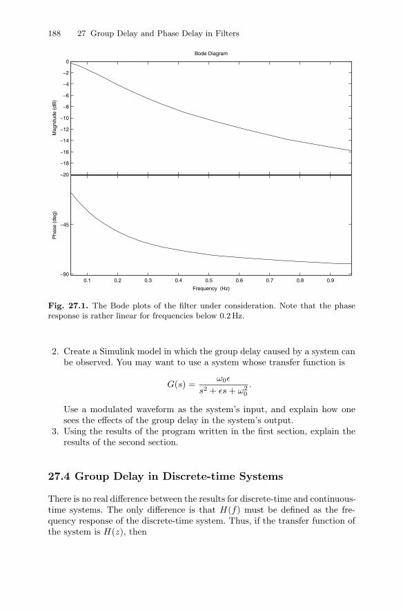
188 27 Group Delay and Phase Delay in Filters
−20
−18
−16
−14
−12
−10
−8
−6
−4
−2
0
Mag
nitu
de (
dB)
0.1 0.2 0.3 0.4 0.5 0.6 0.7 0.8 0.9−90
−45
Pha
se (
deg)
Bode Diagram
Frequency (Hz)
Fig. 27.1. The Bode plots of the filter under consideration. Note that the phaseresponse is rather linear for frequencies below 0.2 Hz.
2. Create a Simulink model in which the group delay caused by a system canbe observed. You may want to use a system whose transfer function is
G(s) =ω0ε
s2 + εs + ω20
.
Use a modulated waveform as the system’s input, and explain how onesees the effects of the group delay in the system’s output.
3. Using the results of the program written in the first section, explain theresults of the second section.
27.4 Group Delay in Discrete-time Systems
There is no real difference between the results for discrete-time and continuous-time systems. The only difference is that H(f) must be defined as the fre-quency response of the discrete-time system. Thus, if the transfer function ofthe system is H(z), then
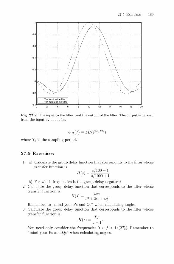
27.5 Exercises 189
0 2 4 6 8 10 12 14 16 18 20−0.4
−0.2
0
0.2
0.4
0.6
0.8
1
The input to the filter.The output of the filter
Fig. 27.2. The input to the filter, and the output of the filter. The output is delayedfrom the input by about 1 s.
ΘH(f) ≡ � H(e2πjfTs)
where Ts is the sampling period.
27.5 Exercises
1. a) Calculate the group delay function that corresponds to the filter whosetransfer function is
H(s) =s/100 + 1s/1000 + 1
.
b) For which frequencies is the group delay negative?2. Calculate the group delay function that corresponds to the filter whose
transfer function isH(s) =
ω0ε
s2 + 2εs + ω20
.
Remember to “mind your Ps and Qs” when calculating angles.3. Calculate the group delay function that corresponds to the filter whose
transfer function isH(z) =
Tsz
z − 1.
You need only consider the frequencies 0 < f < 1/(2Ts). Remember to“mind your Ps and Qs” when calculating angles.
28
Design of FIR Filters
Summary. In Chapter 22, we considered two simple finite impulse response (FIR)filters. We have not yet considered how one goes about designing a generic finiteimpulse response filter. We now remedy that lack.
Keywords. FIR filter design, symmetric FIR filter, windows, Fourier series, group
delay.
28.1 FIR Filter Design
One way of designing a filter is to take the desired frequency response andfind the precise set of coefficients that gives one such a filter. As we will see,the coefficients that correspond to the most commonly desired filters cannotbe implemented “as is.”
Suppose that one chooses to sample one’s input Ts times per second andthat one would like a filter H(z) whose frequency response is H(f) (betweenf = −Fs/2 and f = Fs/2). That is, one would like
H(e2πjfTs) = H(f).
Generally speaking, we start by requiring that H(f) be real and even.(These properties guarantee that the impulse response of the filer is real andeven. See Exercise 3.) As H(f) is supposed to be the frequency response of adiscrete-time filter, it must be periodic with period Fs = 1/Ts (as we saw inSection 18.10).
Assuming that
H(z) =∞∑
m=−∞hmz−m,
we find that we are looking for coefficients, hm, that satisfy
192 28 Design of FIR Filters
∞∑
m=−∞hme−2πjmfTs = H(f).
The hm are essentially the coefficients of the Fourier series associated withH(f). We find that
hm =1Fs
∫ Fs/2
−Fs/2
e2πjmfTsH(f) df.
As we know that the hm are even in m, we know that the filter we aredesigning is not going to be a causal filter—its response to a delta functionprecedes the arrival of the delta function. We deal with this problem shortly.
Let us consider a simple design example. Suppose that one would likeTs = 1ms, and one would like a filter that passes all frequencies up to 100Hz.That is, H(f) = 1 for |f | ≤ 100, and it is zero otherwise. We find that form �= 0,
hm = 0.001∫ 500
−500
e2πjmf/1000H(f) df
= 0.001∫ 100
−100
e2πjmf/1000 df
=0.001
2πjm/1,000
(e2πjm/10 − e−2πjm/10
)
=sin(2πm/10)
πm.
When m = 0, a simple calculation shows that h0 = 0.2.We find that the coefficients are real and even. Additionally, they extend
from m = −∞ to ∞. Clearly, they do not correspond to a finite impulseresponse filter. In order to transform our filter into a finite impulse responsefilter, we set all the filter coefficients for which |m| > M to zero. That is, weconsider the approximation to the ideal filter given by
G(z) =M∑
m=−M
hmz−m.
What effect does “zeroing” all the coefficients that affect samples far fromthe current one have? What we have just done is to take a set of filter coeffi-cients and multiply them by a sequence that is one for |m| ≤ M and that iszero elsewhere. Defining the window sequence wm = 1 for |m| ≤ M , and zerootherwise, we find that the coefficients of the new filter are hmwm.
It is not hard to see that multiplying the coefficients in the “time” do-main is equivalent to convolution in the frequency domain. Consider two Z-transforms, H(z) and G(z), having regions of convergence that include theunit circle. Let us consider the convolution of H(e2πjfTs) with G(e2πjfTs)
28.1 FIR Filter Design 193
H(e2πjfTs) ∗ G(e2πjfTs) ≡∫ Fs/2
−Fs/2
H(e2πjφTs)G(e2πj(f−φ)Ts) dφ.
A quick calculation shows that
H(e2πjfTs) ∗ G(e2πjfTs) =∫ Fs/2
−Fs/2
H(e2πjφTs)G(e2πj(f−φ)Ts) dφ
=∫ Fs/2
−Fs/2
( ∞∑
n=−∞e−2πjn(f−φ)Tsgn
)×
( ∞∑
m=−∞e−2πjmφTshm
)dφ
=∞∑
n=−∞
∞∑
m=−∞
∫ Fs/2
−Fs/2
e−2πjn(f−φ)Tsgne−2πjmφTshm dφ
=∞∑
n=−∞e−2πjnfTsgn ×∞∑
m=−∞
∫ Fs/2
−Fs/2
e−2πj(m−n)φTshmgn dφ
=∞∑
n=−∞e−2πjnfTsgn
∞∑
m=−∞Fsδm−nhm
= Fs
∞∑
n=−∞e−2πjnfTsgnhn.
This is Fs times the frequency response of the system whose coefficients arehngn.
In order to determine the effect of the windowing procedure, we must findthe function W (e2πjfTs) associated with the coefficients wm. By definition(and after some calculation), we find that
W (e2πjfTs) =∞∑
k=−∞wke−2πjfkTs
=M∑
k=−M
e−2πjfkTs
= e2πjMTs
2M∑
k=0
e−2πjfkTs
= e2πjMTs1 − e−2πjf(2M+1)Ts
1 − e−2πjfTs
=sin(π(2M + 1)fTs)
sin(πfTs).
194 28 Design of FIR Filters
This function is very similar to the sinc function. As M becomes larger, thefunction tends to Ts times a periodic delta function (as seen in Section 1.2).
When one convolves H(f) with W (e2πjfTs), one finds that the resultingfunction is a smeared version of H(f) that has sidelobes that surround theareas in which the filter response is supposed to be one. As in the case ofthe calculation of the DFT, the sidelobes are larger when W (e2πjfTs) itselfhas large sidelobes—when it does not decay quickly away from f = 0. This,it can be shown, happens when wm has large abrupt changes. (And this isprecisely what we saw in Chapter 5 when we considered the effect that awindow has on the DFT of a sequence.) Thus, just as in the case of theDFT, it can be advantageous to use a window function that does not changetoo abruptly—for example, a raised-cosine (Hann) window. When we usedwindows to help remove spurious high-frequency terms from the DFT, wefound that window functions generally widen the peaks one should see inthe DFT. In the case of FIR filter design, window functions generally makethe transition from passband to stopband less sharp—and that is a problemcaused by using window functions.
In Figure 28.1, MATLAB r© code that compares the frequency response ofthe filter designed in Section 28.1 with the frequency response of a filter thatuses a windowed version of the same coefficients is given. The figure generatedby the code is given in Figure 28.2. We find that the filter implemented withoutwindowing the coefficients has a frequency response with rather pronouncedripple. On the other hand, the frequency response after windowing has a widertransition region.
28.2 Symmetric FIR Filters
If we desire to build a filter that selects certain frequency ranges and that hasa constant group delay, then the symmetric FIR filter is often a good solution.A symmetric FIR filter is most reasonably defined as an FIR filter for which
h−n = hn.
We have seen that if the frequency response we are trying to achieve, H(f),is real and even, then hn will be real and even as well. Let us consider thetransfer function of a symmetric FIR filter. We find that
H(z) =M∑
m=−M
hmz−m.
Substituting z = e2πjfTs , we find that the frequency response of the filter is
H(e2πjfTs) =M∑
m=−M
hm(e2πjfTs)−m
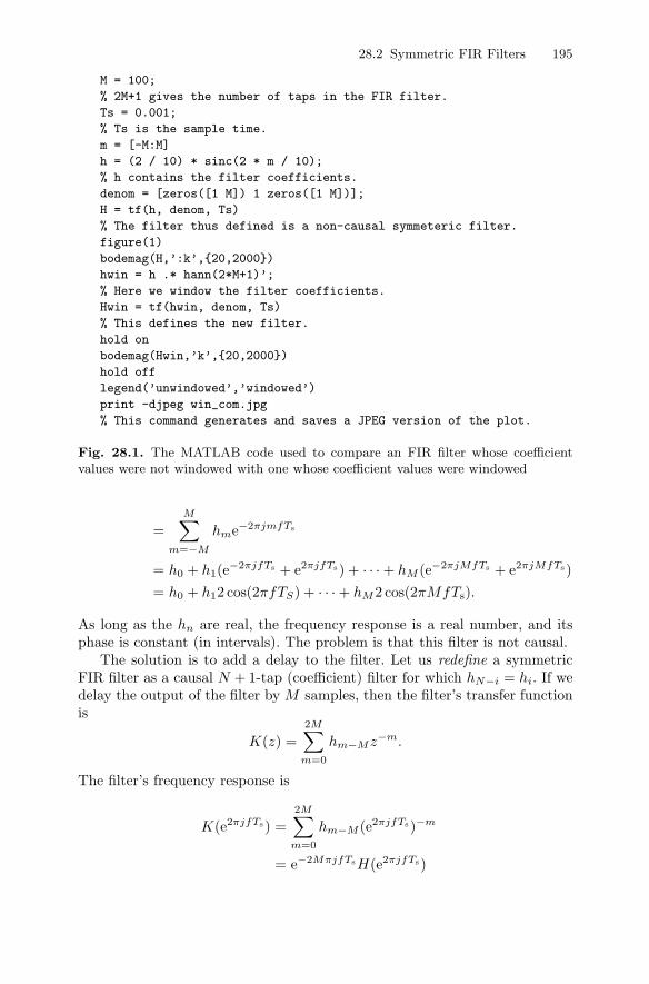
28.2 Symmetric FIR Filters 195
M = 100;
% 2M+1 gives the number of taps in the FIR filter.
Ts = 0.001;
% Ts is the sample time.
m = [-M:M]
h = (2 / 10) * sinc(2 * m / 10);
% h contains the filter coefficients.
denom = [zeros([1 M]) 1 zeros([1 M])];
H = tf(h, denom, Ts)
% The filter thus defined is a non-causal symmeteric filter.
figure(1)
bodemag(H,’:k’,{20,2000})
hwin = h .* hann(2*M+1)’;
% Here we window the filter coefficients.
Hwin = tf(hwin, denom, Ts)
% This defines the new filter.
hold on
bodemag(Hwin,’k’,{20,2000})
hold off
legend(’unwindowed’,’windowed’)
print -djpeg win_com.jpg
% This command generates and saves a JPEG version of the plot.
Fig. 28.1. The MATLAB code used to compare an FIR filter whose coefficientvalues were not windowed with one whose coefficient values were windowed
=M∑
m=−M
hme−2πjmfTs
= h0 + h1(e−2πjfTs + e2πjfTs) + · · · + hM (e−2πjMfTs + e2πjMfTs)= h0 + h12 cos(2πfTS) + · · · + hM2 cos(2πMfTs).
As long as the hn are real, the frequency response is a real number, and itsphase is constant (in intervals). The problem is that this filter is not causal.
The solution is to add a delay to the filter. Let us redefine a symmetricFIR filter as a causal N + 1-tap (coefficient) filter for which hN−i = hi. If wedelay the output of the filter by M samples, then the filter’s transfer functionis
K(z) =2M∑
m=0
hm−Mz−m.
The filter’s frequency response is
K(e2πjfTs) =2M∑
m=0
hm−M (e2πjfTs)−m
= e−2MπjfTsH(e2πjfTs)
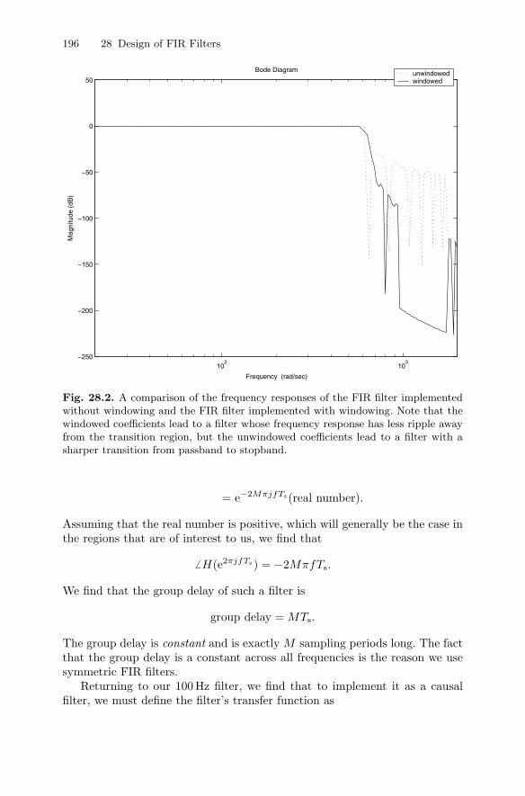
196 28 Design of FIR Filters
102
103
−250
−200
−150
−100
−50
0
50
Mag
nitu
de (
dB)
unwindowedwindowed
Bode Diagram
Frequency (rad/sec)
Fig. 28.2. A comparison of the frequency responses of the FIR filter implementedwithout windowing and the FIR filter implemented with windowing. Note that thewindowed coefficients lead to a filter whose frequency response has less ripple awayfrom the transition region, but the unwindowed coefficients lead to a filter with asharper transition from passband to stopband.
= e−2MπjfTs(real number).
Assuming that the real number is positive, which will generally be the case inthe regions that are of interest to us, we find that
� H(e2πjfTs) = −2MπfTs.
We find that the group delay of such a filter is
group delay = MTs.
The group delay is constant and is exactly M sampling periods long. The factthat the group delay is a constant across all frequencies is the reason we usesymmetric FIR filters.
Returning to our 100 Hz filter, we find that to implement it as a causalfilter, we must define the filter’s transfer function as
28.4 The Experiment 197
H(z) =2M∑
m=0
hm−Mz−m.
This filter is causal and, other than a linearly varying phase, has the desiredfrequency response.
28.3 A Comparison of FIR and IIR Filters
Were it not for the fact that both FIR and IIR filters have their places, oneor the other type of discrete-time filter would have been forgotten long ago.FIR filters have two major advantages
1. Symmetric FIR filters have linear phase—and hence the group delay isthe same at all frequencies.
2. FIR filters are always stable.
IIR filters, though their phase response is not ideal and they can be un-stable have one major advantage: They generally require many fewer taps intheir implementation. When using a resource-poor microprocessor, one mayfind that IIR filters are appropriate. For an interesting discussion that con-siders many of these points, the reader may wish to consult [16].
28.4 The Experiment
Let us use MATLAB r© to start experimenting with FIR filter design. Usethe MATLAB command fdatool (and the GUI it opens for you) to design abandpass filter with 99 taps whose passband extends from 25 to 35 Hz. Makethe sampling frequency of the filter 200 samples s−1.
When you set up fdatool, make sure to select a bandpass filter, makesure that the filter is an FIR filter, and make sure that the design methodyou choose is “Window.” Use several different windows in your design, andprint out the frequency response you achieve with each window. Also, analyzethe impulse response of the filters. Explain why you see the types of impulseresponses you obtain.
Finally, design a nine- or ten-tap bandpass filter that samples at a rate of1,350 samples s−1 and that passes all frequencies in the range extending from135 to 270 Hz. Window the filter coefficients to keep the frequency responseof the filter near zero in the regions where the frequency response is supposedto be zero. Implement the filter on the ADuC841 using a C program, andexamine the properties of the filter that has been implemented.

198 28 Design of FIR Filters
28.5 Exercises
1. Explain what “least squares” FIR filter design is. Feel free to use thelibrary, the web, or any of the various MATLAB “help” features to acquirethe information necessary to answer this question.
2. a) Design a 201-tap symmetric high-pass FIR filter for which• Ts = 500μs, and• the cut-off frequency is 400 Hz.
b) Have MATLAB calculate and plot the Bode plots corresponding tothis filter.
c) Now, multiply the coefficients by a Hanning window of the appropriatesize, and have MATLAB plot the Bode plots of the new filter. Howdo the new plots compare to those of the unwindowed filter?
3. Please show that for any real even function, the coefficients, bk, are realand satisfy bk = b−k—they are symmetric in k. You may wish to proceedby showing that for any real function, b−k = bk. Then, you may wish toshow that for any even function, bk = b−k.
29
Implementing a Hilbert Filter
Summary. Though many of the filters that we use are frequency-selective—theypick out frequencies that are for one reason or another important to us—not allfilters are of this type. Here, we consider the Hilbert filter—an all-pass filter.
Keywords. Hilbert filter, all-pass filter, Fourier series.
29.1 An Introduction to the Hilbert Filter
The frequency response desired of an analog Hilbert filter, H(f), is
H(f) =
⎧⎨
⎩
j, f < 00, f = 0
−j, f > 0.
When implementing the filter digitally, the desired frequency response is
H(Ω) =
⎧⎨
⎩
j, −π < Ω < 00, Ω = 0
−j, 0 < Ω < π
where Ω = 2πfTs. As this is a discrete-time filter, we know that if {hk} arethe filter coefficients, then the filter’s frequency response is
frequency response =∞∑
k=−∞hke−jΩk.
We choose {hk} such that the frequency response of the filter equals thedesired frequency response:
∞∑
k=−∞hke−jΩk = H(Ω).
200 29 Implementing a Hilbert Filter
As expected, we find that the hk are (essentially) the Fourier coefficients ofH(Ω).
Clearly,
hk =12π
∫ π
−π
H(Ω)ejΩk dΩ
=1π
∫ π
0
sin(Ωk) dΩ
=1π
cos(0) − cos(πk)k
={
2πk k odd0 k even .
Thus, the transfer function of the filter is
H(z) =∞∑
k=−∞hkz−k =
2π
∞∑
k=−∞
12k + 1
z−(2k+1). (29.1)
29.2 Problems and Solutions
As seen in Chapter 28, there are two problems associated with implementingthis filter
1. the filter is not causal, and2. the impulse response is infinite.
We take care of these problems by truncating the response and delaying it. Weapproximate the Hilbert filter by considering a filter whose transfer functionis
HN (z) =2π
z−(2N−1)N−1∑
k=−N
12k + 1
z−(2k+1), N ≥ 1.
29.3 The Experiment
Implement the filter whose transfer function is H3(z) on the ADuC841. Usea sampling rate of 2,700 samples s−1. In addition to outputting the output ofthe filter via DAC0, use DAC1 to output the input to the filter, but delay theinput by five samples. Compare the output of the two DACs to see the −90o
phase shift introduced by the filter. Print out several oscilloscope traces, andinclude them with your laboratory report.
29.4 Exercises 201
29.4 Exercises
1. Use MATLAB to show that when N = 5, the filter in Section 29.2 providesus with the phase response that we desired (except for a linear term addedby the “block” that delays the filter’s output by 2 × 5 − 1 samples).
2. Discuss the Gibbs phenomenon, and show why it implies that approxima-tions of the type we are making will never tend uniformly to the magnituderesponse we want. Show that there will always be points of the magnituderesponse that differ from the desired value by several percent.
3. Is the filter given by (29.1) stable? Explain!
30
The Goertzel Algorithm
Summary. We have seen that the FFT allows one to calculate the DFT of anN -term sequence in O(N ln(N)) steps. As calculating a single element of the DFTrequires O(N) steps, it is clear that when one does not need too many elements of theDFT, one is best off calculating individual elements, and not the entire sequence. Inthis chapter, we present a simple algorithm—the Goertzel algorithm—for calculatingindividual elements of the DFT.
Keywords. Goertzel algorithm, DFT, second-order filter.
30.1 Introduction
Consider the definition of the DFT
Ym = DFT({yk})(m) ≡N−1∑
k=0
e−2πjmk/Nyk.
The calculation of any given coefficient, Ym, takes O(N) steps. Thus, if oneonly needs a few coefficients (fewer than O(ln(N)) coefficients), then it isbest to calculate the coefficients and not bother with the “more efficient”FFT algorithm (which calculates all of the Fourier coefficients). The Goertzelalgorithm1 is a simple way of calculating an individual Fourier coefficient. Itturns calculating a Fourier coefficient into implementing a second-order filterand using that filter for a fixed number of steps. The Goertzel algorithm issomewhat more efficient than a “brute force” implementation of the DFT.
30.2 First-order Filters
Consider the solution of the equation1 Named after its discoverer, Gerald Goertzel. The algorithm was published in 1958
[11].
204 30 The Goertzel Algorithm
rn = αrn−1 + xn. (30.1)
This corresponds to calculating the response of the filter whose transfer func-tion is
R(z)X(z)
=z
z − α.
Making use of the variation of parameters idea [17], we guess that thesolution of (30.1) is of the form
rn = αnzn.
We find that we must produce a zn for which
rn = αnzn
= αrn−1 + xn
= α(αn−1zn−1) + xn
= α(αn−1(zn + (zn−1 − zn)) + xn
= αnzn + αn(zn−1 − zn) + xn.
In order for equality to hold, we find that
zn = zn−1 + α−nxn. (30.2)
Assuming that rn = xn = 0 for n < 0, (30.2) implies that
zn =n∑
k=0
α−kxk.
Finally, we find that
rn = αnzn =n∑
k=0
αn−kxk. (30.3)
(For another way of arriving at this result, see Exercise 3.)
30.3 The DFT as the Output of a Filter
Let us consider the definition of the DFT again. We find that
Ym =N−1∑
k=0
e−2πjmk/Nyk
=N−1∑
k=0
(e2πjm/N )N (e−2πjm/N )kyk.
30.4 Comparing the Two Methods 205
=N−1∑
k=0
(e2πjm/N )N−kyk
= e2πjm/NN−1∑
k=0
(e2πjm/N )N−1−kyk.
We find that Ym is the output of a first-order filter at “time” N − 1.Let us examine the relevant filter. We find that the filter’s transfer function
is
T (z) =ze2πjm/N
z − e2πjm/N.
This transfer function can be rewritten as
T (z) =z(ze2πjm/N − 1)
z2 − 2z cos(2πm/N) + 1.
This transfer function can be considered the product of two transfer functions,T1(z)T2(z), where
T1(z) =1
1 − 2z−1 cos(2πm/N) + z−2, and T2(z) = e2πjm/N − z−1.
We find that the first transfer function has real coefficients, and the secondcorresponds to a finite impulse response filter. As the output of the secondfilter is needed only when k = N − 1, the FIR filter need not be implementedexcept at that last step.
We can calculate Ym by implementing the filter
rn = 2rn−1 cos(2πm/N) − rn−2
and continuing the calculation until n = N − 1. At that point, we calcu-late Ym = e2πjm/NrN−1 − rN−2. This algorithm is known as the Goertzelalgorithm.
30.4 Comparing the Two Methods
To what extent is the Goertzel algorithm more efficient than the direct calcu-lation of the value of Ym,
Ym =N−1∑
k=0
e−2πjmk/Nyk?
If one performs a brute force calculation of Ym, one must multiply e−2πjmk/N
by yk for N values of k. As the complex exponential is essentially a pair of real
206 30 The Goertzel Algorithm
numbers, this requires 2N real multiplications. Additionally, the sum requiresthat 2(N − 1) real sums be calculated. When using the Goertzel algorithm,the recurrence relation requires two real additions and one real multiplicationat each step. The FIR filter that is used in the final stage requires two realmultiplications and one addition. In sum, the Goertzel algorithm requiresN +2 real multiplications and 2N +1 real additions. We find that the Goertzelalgorithm is somewhat more efficient than the brute force calculation.
30.5 The Experiment
Implement the Goertzel algorithm using Simulink r©. Calculate one of theelements of the FFT of a sequence that is 16 elements long.
1. Implement the filter T1(z). As its coefficients are all real, this is not aproblem.
2. Implement filter T2(z) as two separate filters. One should produce the realpart of the FFT, and the second should produce the imaginary part.
3. Let the input to the filters come from the workspace, and let the outputof each of the filters go to the workspace. (Look at the Simulink sourcesand sinks to find the appropriate blocks.)
4. Try out the final set of filters with a variety of inputs. Note the size of theoutput of the filter T1(z).
5. In your report, explain why implementing the Goertzel algorithm using amicroprocessor might be challenging.
30.6 Exercises
1. Discuss the stability of filter T1(z).2. Why are we able to use T1(z) even though it is a “problematic” filter?
Explain your answer clearly.3. Show that (30.3) describes the relation between xn and rn by using the
fact that the operations being described are causal, by assuming thatxn = 0 when n < 0, and by making use of the Z-transform.
References
1. Aziz, P.M., Sorensen, H.V., and van der Spiegel, J., “An Overview of Sigma–Delta Converters,” IEEE Signal Processing Magazine, Vol. 13, No. 1, 1996.
2. Bennett, S., “Control Systems: The Classical Years 1935-1955,”http://www.mech.gla.ac.uk/Research/Control/Seminars/bennett.html,accessed June 7, 2007.
3. Churchill, R. V., Brown, J. W., and Verhey, R. F., Complex Variables and Ap-plications, 3rd edn., McGraw-Hill, New York, 1976.
4. Constantinides, A., “Spectral Transformations for Digital Filters,” Proc. IEEE,Vol. 117, No. 8, 1970.
5. Cooley, J.W., and Tukey, J.W., “An Algorithm for the Machine Calculation ofComplex Fourier Series,” Math. Comput., Vol. 19, 1965.
6. Engelberg, S., A Mathematical Introduction to Control Theory, Series in Elec-trical and Computer Engineering, Vol. 2, Imperial College Press, London, 2005.
7. Engelberg, S., Random Signals and Noise: A Mathematical Introduction, CRCPress, Boca Raton, FL, 2006.
8. Engelberg, S., “Implementing a Sigma–Delta DAC in Fixed Point Arithmetic,”IEEE Signal Processing Magazine, Vol. 23, No. 6, 2006.
9. Engelberg, S., A Microprocessor Laboratory Using the ADuC841, JerusalemCollege of Technology, Jerusalem, Israel, 2007, http://www.springer.com/978-1-84800-118-3.
10. Frantz, G. and Simar, R., “DSP: Of Processors and Processing,” ACM Queue,Vol. 2, No. 1, 2004,http://acmqueue.com/modules.php?name=Content&pa=showpage&pid=125,accessed November 12, 2007.
11. Goertzel, G., “An Algorithm for the Evaluation of Finite Trigonometric Series,”American Mathematical Monthly, Vol. 65, No. 1, 1958.
12. Jung, W., Editor, Op Amp Applications Handbook, Newnes, Burlington, MA,2005, http://www.analog.com/library/analogDialogue/archives/39-05/op amp applications handbook.html, accessed June 11, 2006.
13. Keil Elektronik GmbH., Cx51 Compiler: Optimizing C Compiler and LibraryReference for Classic and Extended 8051 Microcontrollers, 1988-2000.
14. Oppenheim, A.V., and Schafer, R.W., Digital Signal Processing, Prentice-Hall,Englewood Cliffs, NJ, 1975.

208 References
15. Oppenheim, A.V., Willsky, A.S., and Young, I.T., Signals and Systems, Prentice-Hall, Englewood Cliffs, NJ, 1983.
16. Rader, C.M., “DSP History – The Rise and Fall of Recursive Digital Filters,”IEEE Signal Processing Magazine, Vol. 23, No. 6, 2006.
17. Thomas, G.B., Calculus and Analytic Geometry, 4th edn., Addison Wesley,Reading, MA, 1968.
18. Wikipedia, the free encyclopedia, http://en.wikipedia.org, accessed November22, 2007.
19. Zemanian, A.H., Distribution Theory and Transform Analysis, Dover, New York,1987.
Index
8051 143
ADuC841 14, 42, 61, 78, 79, 183, 197,200
C for 143DACs 104FLASH memory
program memory 53maximum output current 78
aliasing 11amplifier
inverting 72non-inverting 72
analog to digital converter 67, 89dual slope 95flash 104oversampling 112pipelined 99
latency of 100throughput of 99
sigma–delta 110single slope 93successive approximation 89
basebanddefinition 17
bilinear transform 160binary search 89biquad 183
definition 177buffer
unity-gain 69, 77
C 143
fprintf command 54Cauchy-Schwarz inequality 23causal system 127Chebyshev polynomials 156circular convolution
definition of 34compact support
definition of 21complex plane
one-to-one and onto mapping of 166convolution 39
of periodic functions 192Cooley, J.W. 35
DAC 68binary weighted 81passive 75R-2R 85resistor-chain 103sigma–delta 113
delta functiondefinition of 122
DFT 29definition 30of random signal
variance of 58properties
almost norm preserving 33convolution 35periodicity 34symmetry 34
digital to analog converter see DACdiscrete convolution
definition of 123
210 Index
Discrete Fourier Transform see DFTdiscrete-time system
frequency response of 131magnitude response of 131
fast Fourier transform see FFTFFT 35filter
3 dB down point 156all-pass 172, 199analog
Butterworth 155Chebyshev 155design of 155elliptic 156maximally flat 155
anti-aliasing 11, 112Butterworth 18
and RC filters 158first-order
discrete-time 203low-pass
RC 61narrow-band bandpass
using feedback to design 151notch 151
filter conversionslow-pass to bandpass 170low-pass to high-pass 167low-pass to low-pass 168
filter designusing MATLAB 181
fully automatic 183finite impulse response filters see FIR
filtersFIR filters 147
comparison with IIR filters 197design of 191
least squares 198group delay of 196high-pass 148low-pass 147running average filter 147stability of 140symmetric 186, 194taps
definition of 147transfer functions of 139
Fourier transform
analyticity 21and lack of compact support 23
definition of 4of ideally sampled function 9
Fubini’s theorem 123
Gauss, C.F. 35geometric series
finite 147Gibbs phenomenon 201Goertzel algorithm 203
filterstability of 206
Goertzel, Gerald 203group delay
continuous time 186
Hilbert filters 199hold
frequency response of 4
IDFT 32IFFT 36IIR filters
comparison with FIR filters 197definition of 139design of 155
from analog prototypes 161first-order 203simple low-pass 143transfer functions of 140
impulse responsedefinition of 122
inverse DFT see IDFTinverse fast Fourier transform see
IFFTinverse Z-transform 124
by contour integration 124by partial fractions expansion 125
Karnaugh map 106Keil μVision3 145
L’hopital’s rule 148LTI
definition of 122
magnitude response 145MATLAB 37
Index 211
and continuous-time transferfunctions 162
commandplot 39
commands’ 49.’ 50.* 41hold on 162abs 38arrays 38bode 132, 145, 164, 182, 187bodemag 133, 167butter 181dec2hex 54fdatool 183, 197fft 37fprintf 54impulse 133legend 162ones 41, 43psd 59, 61rand 54, 61real 43residue 126semicolon 38step 133, 182subplot 39tf 132, 182, 187title 39useful with serial port 42wintool 51zeros 41, 43
example programfor calculation of averaged
periodograms 59for calculation of DFT 38for FIR filters 194
maximum modulus principle 165method of averaged periodograms 59multiplexer 104
Nyquist frequency 10Nyquist sampling theorem 3, 10
op-amp 69golden rules 71
operational amplifier see op-amp
Parseval’s theorem 24, 27periodogram
definition 58phase delay
continuous time 186poles
inside the unit circleand stability 128
simpledefinition of 128
polynomialsChebyshev 156
power spectral density 59, 111prewarping 161, 164PSD see power spectral density
quantization noise 110distribution of 111power spectral density of 111
random variables 105IID 57
realizationscascaded biquads 177direct form I 174direct form II 175
recurrence relation 128initial conditions for 129
residuesmethod of 24
ripplein filter transfer functions 156
sample-and-hold 3, 91sampled-data systems
general structure 67sampler
ideal 3series
alternating 19Taylor 19
sidelobe 46sigma–delta converters
bits of accuracy 112noise shaping 109
signal generator 53Simulink 18sinc function
definition of 45spectral leakage 46
212 Index
square integrable 26stability
condition for 128summer
transfer function of 124superposition
principle of 75, 85, 86, 122, 139
tapfilter 195
thermometer code 104transfer function
definition of 123proper 129, 175
definition of 129triangle inequality 118
application of 13for sums 7
Tukey, J.W. 35
uncertainty principle 23, 46undersampling 14uniform convergence 21unit step function
discrete-time 120unit-circle preserving mappings 166
variation of parameters 204
virtual ground 72, 81, 93
white noise generator 54window function 47
Bartlett 48comparison of several 50Hann 49Hanning 49in FIR filter design 192rectangular 48roll-off of 50
windowing 47and zero-padding 50
Z-transform 117bilateral
definition 117of a two-sided exponential 122of the exponential 121of the sine function 121of the unit step 120ROC
definition 118zero-padding
and windowing 50for spectral interpolation 41in order to utilize the FFT 41to calculate the convolution 39