engineering design & analysis ltd
TRANSCRIPT

EDA Page 1 of 24
EDAEngineering Design & Analysis Ltd
THE FINITE ELEMENT METHOD
A short tutorial giving an overview of the history, theory and application of the finite element method.
Introduction
Value of FEM
Applications
Elements of FEMMesh GenerationElement EquationsAssembly & Matrix Solution MethodsError MinimizationValidation
Using an FEA Program
OrganizationGeometry DefinitionStatic Analysis
Finite Element Library
Plate ExampleOther Examples
Disclaimer!
This tutorial is not a substitute for detailed study of the body of knowledge of the finite element methodology.

EDA Page 2 of 24
FEM – The Finite Element Method
The FEM is a computer aided mathematical technique for obtaining numerical solutions to the abstract equiations of calculus that predict the response of physical systems subjected to external influences.
The FEM solution may be exact for the approximated model of the real system.
Finite Element vs Finite Difference
Finite Difference
o Used for problems dealing with time only as independent variableo Mathematical technique based on power (Taylor) series expansion
o The increments or elements are of equal size, where “h” = (x-a)
The “h” are of fixed size
Finite Element
o Deals with both space (x, y, z) and time (t) as independent variables
o Mathematical technique based on intricate use of algebraic expressions and optimizing techniques
o Elements can vary in size within the domain of the system
.......)("!2
)(')()(2
afh
afhafxf

EDA Page 3 of 24
Historical Background
Notes:
(1) Used framework of physically separate 1D rods and beams to model elastic behaviour of a continuous plate
(2) Used assembly of triangular panels to model complete aircraft wing panel; used all the methodological elements of modern day FEM

EDA Page 4 of 24
Value of FEM for Plant Facilities
Predictive Design, reliability of proposed facilities reduce prototyping
Confirmation Quantify, assess evaluate existing condition
Plant Support Areas
o Engineering - damage and remaining life assessments
o Construction - evaluate construction methods
o Maintenance - evaluate maintenance methods
o Inspection - codes & standards compliance
Equipment Applications
o Pressure vesselso Piping (special purpose FEM programs)o Steam generating equipment, fired heaterso Rotating equipment (pressure containing components)o Tankageo Valving, specialty & commodityo Structureso Heavy lift cranes, draglineso Refractory systemso Equipment auxiliaries
Bellows Dampers Fans Internal structures Stacks
Cost / Benefit
o FEM provides a means to quantify the performance of mechanical / structural equipment against a set of decision criteria such as
design & construction codes monetary cost safety reliability
o The results of properly conducted FEA are accepted by facility insurer’s jurisdiction authorities, and industry owners

EDA Page 5 of 24
Discipline Applications
Solid Mechanics
o Elasticityo Plasticityo Staticso Dynamics
Heat Transfer
o Conduction o Convection o Radiation
Fluid Mechanics
o Laminaro Turbulent
Acoustics
Electromagnetism
Solid State Physics
Quantum Mechanics

EDA Page 6 of 24
FEM Example: Solid mechanics, plasticity (transient dynamic, nonlinear)

EDA Page 7 of 24
FEM Example: Solid mechanics, elastic (static, linear)
Note – this example shows validation of the theoretical results using experimentally determined results.

EDA Page 8 of 24
Why is FEM generally applicable to physical phenomena?
Consider one-dimensional boundary value problems

EDA Page 9 of 24
The Elements of FEM
Mesh generationBoundary ConditionsLoading
Element EquationsAssemblyMatrix Solution Methods
Determine stressesDisplayPrintCombine load cases
pre - processing
computation
post – processing

EDA Page 10 of 24
Mesh Generation
Superficially, mesh generation divides the domain of our system into elements. Associated with each element is a trial function(s) of algebraic expression. The element could be as large asabuilding or as small as small as the chip in a computer CPU. Hence, the term “finite” is used to describe the element.
If u(x) is the exact soluion to our problem, then ũ(x:a) represents an approximate solution in algebraic form where:
ũe(x:a) = a1eØ1
e(x) + a2eØ2
e(x) + …… ane Øn
e(x)
The Øn(x) are set to form a Lagrange interpolation polynomial, i.e. when
Ø1(x) = 1 Ø2(x) = 0, and
Ø1(x) = 0 Ø2(x) = 1
This allows the ane to constrain the equation of ũ(x) to u(x) for all elements
If we let Kij = Kij[Øn(x)], Fi = Fi(Øn)
Then
[Kij] [an] = [Fi]
[K] = Matrix of coefficients that multiply the vector of unknown parameters
[a] = Unknown parameters dependent on the boundary conditions –i.e. sets the DOF, degree of freedom for the solution matrix
[F] = Load vector representing the exterior boundary and interior conditions
EDA Page 11 of 24
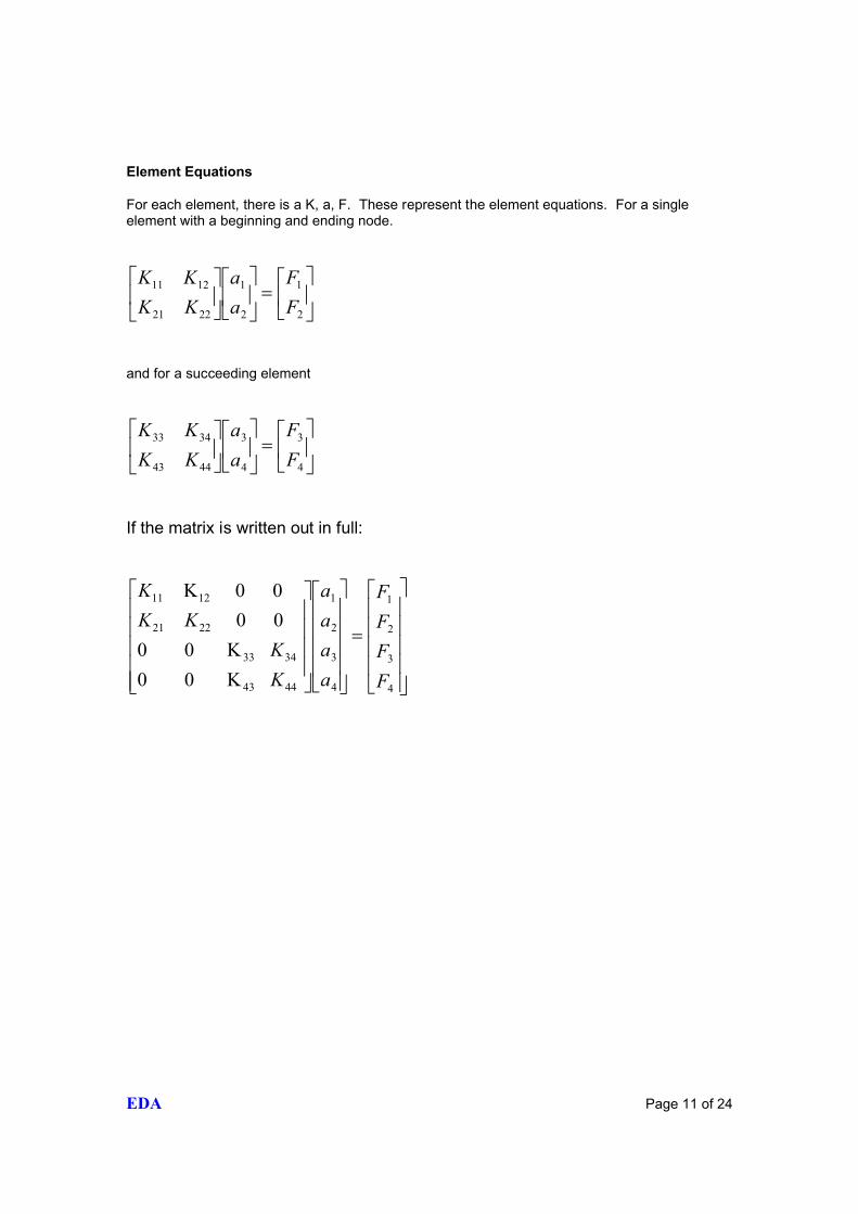
Element Equations
For each element, there is a K, a, F. These represent the element equations. For a single element with a beginning and ending node.
2
1
2
1
2221
1211
F
F
a
a
KK
KK
and for a succeeding element
4
3
4
3
4443
3433
F
F
a
a
KK
KK
If the matrix is written out in full:
4
3
2
1
4
3
2
1
4443
3433
2221
1211
K0 0
K0 0
0 0
0 0 K
F
F
F
F
a
a
a
a
K
K
KK
K

EDA Page 12 of 24
Assembly
For continuity, u1 = u2 at their common node point, i.e. where the elements connect. For our two element matrix, the means a2 = a3. The previous matrix can now be written as:
4
32
1
4
2
1
4443
34332221
1211
K 0
K
0 K
F
FF
F
a
a
a
K
KKK
K
This is known as assembly.
Matrix Solution Methods
As individual element equations are gathered into the system matrix, it is apparent that many zero terms arise; the non-zero terms being located on the main matrix diagonal. Since the non-zero terms predominate, the matrix is said to be sparse and allows for easy solution for the an. The width of the non-zero terms on the diagonal is called the bandwidth.
Once the system equations are assembled, each an is determined by Gaussian elimination.
Once the an have been determined, back substitute into the appropriate solution:
ũe(x:a) = a1e Ø1
e(x) + a2e Ø2
e(x) + …… ane Øn
e(x)
For each element, what does the ũe(x:a)’s represent?
Temperature heat flow
Displacement stress
Voltage current
Hydraulic head fluid flow

EDA Page 13 of 24
Techniques for minimizing error
Convergence
Convergence checks that the answer is unique
Element labelling should ensure that most of the matrix coefficients end up on the main diagonal. Most programs ignore terms outside a bandwidth of 10.
Refine mesh between successive runs and determine convergence
Mesh refinement - “h” method
Increase equations - polynomial trial solutions- complex elements- “p” method
Check continuity across elements for flux terms
Use alternate elements
Validation
Validation checks that the answer is close to the exact solution
Compare answers to known set of answers [benchmark problems]
Determine solution accuracy for simple models with closed form solution
Caution: Error improvement cannot take place if only a few of the mesh elements become arbitrarily small the large elements will have introduced some errors already.

EDA Page 14 of 24
Using an FEA program
Many engineering problems can be analyzed on microcomputers and allow for many design iterations sometimes, too many since the computational time is shortened drastically for many practical problems encountered in an industrial setting.
All input data are entered through the use of menus which correspond to the program modules –
Geometry definition Static analysis Modal analysis Dynamic analysis

EDA Page 15 of 24
Geometry Definition Menu Organization

EDA Page 16 of 24
Static Analysis Menu Organization

EDA Page 17 of 24
FEA Element Library
A typical program element library will provide sufficient elements types to conduct analyses to varying degrees of complexity in the discipline of interest, i.e. structures, fluids, electromagnetism, acoustics, etc.

EDA Page 18 of 24
Example of Static & Dynamic Analysis of a Plate
Static Example:

EDA Page 19 of 24
Displacement Plot
Solution
Deflection % Difference
Software 0.00386 0.8
Theory 0.00383 -
Reference: W.C. Young, “Roark’s Formula’s for Stress and Strain”, 6th Ed pg. 458

EDA Page 20 of 24
Detailed Calculation of Example Static Problem

EDA Page 21 of 24
Dynamic Example
Solution
f1 f2 f3
Software 118.1 295.3 295.3
Theory 119.2 298.3 298.3
% Difference 0.8 1.0 1.0
Reference: W.C. Young, “Roark’s Formulas for Stress and Strain”, 6th Ed. Pg. 717

EDA Page 22 of 24
Dynamic Example [cont’d]
Mode 3
Solution
f1 f2 f3
Software 118.1 295.3 295.3
Theory 119.2 298.3 298.3
% Difference 0.8 1.0 1.0
Reference: W.C. Young, “Roark’s Formulas for Stress and Strain”, 6th Ed. Pg. 717

EDA Page 23 of 24
Detailed Calculation of Example Dynamic Problem

EDA Page 24 of 24
Examples from actual problems
Vessel Top Head with Adjacent Nozzle – overlap of stresses around openings
Outlet Nozzle with Repad – note lack of penetration at repad ID weld