Engineering Fracture Mechanics 126 (2014) 178–189

Contents lists available at ScienceDirect

Engineering Fracture Mechanics

journal homepage: www.elsevier .com/locate /engfracmech

Fluctuations of the dynamic fracture energy values related tothe amount of created fracture surface

http://dx.doi.org/10.1016/j.engfracmech.2014.05.0140013-7944/� 2014 Elsevier Ltd. All rights reserved.

⇑ Corresponding author. Tel.: +33 680041047.E-mail address: jbkopp@unistra.fr (J.-B. Kopp).

Jean-Benoît Kopp a,⇑, Jean Schmittbuhl b, Olivier Noel c, Jian Lin a, Christophe Fond a

a ICube, Université de Strasbourg, 2 rue Boussingault, F67000 Strasbourg, Franceb EOST, Université de Strasbourg, 5 rue René Descartes, F67000 Strasbourg, Francec IMMM, Université du Maine, Avenue Olivier Messiaen, F72085 Le Mans, France

a r t i c l e i n f o a b s t r a c t

Article history:Received 1 October 2013Received in revised form 30 April 2014Accepted 28 May 2014Available online 7 June 2014

Keywords:Dynamic fracturePolymersEnergy release rateRapid crack propagationSurface roughness

Several strip band fracture tests have been performed with rubber toughened polymethyl-methacrylate (RT-PMMA) samples. Using different types of profilometer, the preciseamounts of created surfaces for different locations along the fracture were measured bothbefore and after branching at different scales. It was observed that the fluctuations of thedynamic fracture energy that could be of the order of 300%, are well explained by the fluc-tuations of the actual amount of created surface when the fracture roughness is sampled ata scale of the order of 0.1 lm. This study shows that the classic approach, which approxi-mates the amount of created surface during propagation as a flat rectangle defined as thesample thickness multiplied by the crack length, is not appropriate for a convenientestimate of fracture energy. Indeed, it is shown that the real 3D topography of the createdsurface has to be included in the energy balance to quantify an intrinsic material fractureenergy. If not, fracture energy can be significantly underestimated.

� 2014 Elsevier Ltd. All rights reserved.

1. Introduction

Classically, two kinds of behaviour have been observed concerning rapid crack propagation in materials. On the one hand,there are materials where fracture energy increases with crack tip velocity. In this case, fracture velocity changes duringcrack propagation according to available energy i.e. the dynamic energy release rate GId. A difference in velocity beforeand after branching is observed and the main crack propagates faster than the secondary cracks after branching [1–3]. Onthe other hand, there are materials where the fracture energy tends to decrease with crack tip velocity. They are viscoplasticblend materials and polymers [4,5] such as rubber toughened polymethylmethacrylate (RT-PMMA) or many semi-crystallines [6,7]. Crack tips for these materials are seen to propagate at the same macroscopic velocity in mode I solicitationno matter the dynamic energy release rate [8–10]. Crack tip velocity is also the same along secondary branches. Creep crackgrowth behaviour may be observed at low velocities below 0:001cr , where cr is the Rayleigh wave speed. In the rangebetween, approximately, 0:01cr and 0:6cr , no crack propagation was observed in RT-PMMA. Crack tip propagation is unstablebecause fracture energy is larger in this range [8,11]. In the case of rapid crack propagations, as observed in [8], propagationat macroscopic crack branching velocity is maintained by, on the one hand, the mechanism of immediate crack branching for

Nomenclature

GId the dynamic energy release rate (J/m2)GIdc the dynamic fracture energy (J/m2)GI0 the quasi-static energy release rate (J/m2)Wext: the work done by external forces (J)Wela: the elastic energy (J)Kcin: the kinetic energy (J)Wdis: the bulk dissipated energy (J)cr the Rayleigh waves speed (m/s)_a the crack tip velocity (m/s)a the crack tip position (m)E the dynamic elastic modulus (Pa)m the Poisson coefficient (–)Ar the amount of created fracture surfaceA0 the amount of projected fracture surfaceL.E.F.M the Linear Elastic Fracture MechanicsSBS the strip band specimen geometryRT-PMMA rubber toughened polymethylmethacrylate

J.-B. Kopp et al. / Engineering Fracture Mechanics 126 (2014) 178–189 179

larger velocities and, on the other hand, by fracture energy increasing for lower velocities. These two combined mechanismsrender impossible acceleration or deceleration of the crack tip. Only propagation at 0:6cr or instantaneous crack arrest1 isobserved. Hence, the amount of created surface is expected to evolve with dynamic fracture energy GIdc . Below a minimal valueof GIdc , cracks stop without any decrease in crack tip velocity which is contrary to the first type of materials. The crack arrestphases correspond to relatively smooth fracture surfaces. Moreover, fracture surface roughness is seen to increase with thevalue of dynamic fracture energy at a specific constant velocity corresponding to crack branching velocity.

These observations drive the present study to explore the link between the amount of created fracture surfaces producedduring the fracture propagation and the fracture energy GIdc in the case of a model material: RT-PMMA [12]. The rubbertoughened (RT) polymers which are used have remarkable properties for dynamic fracture. The general principle of RTreinforcement is to dissipate energy throughout the material through elastomer particles in contrast to pure amorphouspolymers where energy dissipation is smaller and more confined at the crack tip. The presence of elastomer particles in apolymer matrix reinforces the initial material against an external impact by a cavitation mechanism, observed by X-rayscattering [13], transmission electron microscopy (TEM) and light scattering [14,15]. Cavitations enlarge the process zoneand enhance plastic dissipation which subsequently decreases the stresses (stress concentration) at the crack tip andincreases fracture energy. However, in rapid crack propagation (RCP) regime, it has been shown that the process zone is con-fined [16–27,6]. Indeed, beyond a loading rate of 1 s�1 elastomer particles fall below glass transition temperature (Tg), owingto the well-known time–temperature equivalence, and recover the mechanical behaviour of a glassy state where they areless able to cavitate. The material becomes as brittle as the pure amorphous polymer matrix and prone to the propagationof dynamic cracks. The formalism of Linear Elastic Fracture Mechanics (L.E.F.M.) can thus be used [16–23]. Several studies onthe mechanical properties of rubber toughened polystyrene (RT-PS) [28–30], RT-PMMA [8,11] or rubber toughened polyam-ide (RT-PA) [31,32] are described in the literature and the use of dynamic L.E.F.M is assessed.

Finally, when applying L.E.F.M. formalism, it is considered that the created surface is the sample thickness multipliedby crack length i.e. a plane surface. The results show that this approximation only accounts for a crude estimate of frac-ture energy GIdc. Indeed, significant fluctuations up to 300% in fracture energy were observed despite constant crack tipvelocity. This paper deals with a link between the fluctuations in GIdc and the amount of created surface because of thechange in fracture roughness with GIdc. Evaluation of the amount of created surface is not a simple task as fractureroughness is known to be multi-scale [33–35]. Therefore, surface measurements are a function of measurement scale.For this reason, several techniques have been successfully used and compared: atomic force microscopy [36] andmechanical profilometer [37].

2. Material and methods

2.1. Samples

The industrial grade RT-PMMA consists of a PMMA matrix containing a volume fraction of approximately 20% of sphericalelastomer particles of about 100 nm in diameter. The manufacturer blends elastomer particles with either fluid or melted

1 The beginning of a creep crack growth regime is considered herein as a crack arrest.

Fig. 1. Sketch of the strip band specimen geometry (SBS) (L ¼ 200� 1 mm, H ¼ 60� 5 mm, T ¼ 2� 0:1 mm) uniformly loaded with imposed displacementsu in mode I. A conductive layer of an Ag (1) with a thickness of approximately 10 lm, is spread on the sample and used to record the crack tip positionduring propagation.

180 J.-B. Kopp et al. / Engineering Fracture Mechanics 126 (2014) 178–189

PMMA at a high temperature. The glass transition temperature (Tg) of the matrix is 105 �C while that of the elastomer par-ticles is about �30 �C.

The strip band specimen geometry (SBS) presented Fig. 1 has been chosen for its moderate ‘dynamic correction’ [38]. Aninitial notch (length a0 � 5

2 H where H is the sample width) is machined into the sample to eliminate border effects as muchas possible.

2.2. Fracture propagation test

Samples are initially pre-stressed in a uni-axial strain using an Instron tensile testing machine equipped with a 150 kNforce cell. The tensile testing machine is only controlled by imposed displacements which are locked after loading. To bereproducible and to be able to neglect the loading rate and the loading time between each sample, the crack is initiated aftera significant relaxation period of typically 15 times the loading time (see Fig. 5). Loading rates could be slightly differentowing to the experimental device. So, the relative loading–relaxation–initiation time can be considered to be the samefor each sample. Initiation of the crack propagation is induced by the impact of a razor blade on the notch tip. The entiretest is performed at a quasi-constant temperature of 23 �C.

A notched and fractured RT-PMMA sample is presented in Fig. 2. It shows an overview of some post-mortem fracturedsamples including the machined notch. The initiation zone is detailed with a zoom around the notch where the materialis whitened by the cavitation of rubber particles which denotes a rubbery state behaviour. After the initiation zone, thereis both dynamic fracture propagation and branching. Branching appears because of inertial effects at an approximate crackvelocity of 0:6cr [39]. Two different branching situations are observed: macro-branching and micro-branching. The size ofthe secondary crack after branching has been used to calculate the difference between these two types of branching.Macro-branching herein denotes secondary crack extension d typically larger than 1 cm and micro-branching for d 6 1 cm.

Two sets of RT-PMMA samples have been used in this study. A first group is devoted to the measurement of crack tipvelocity and the estimate of dynamic fracture energy GIdc. For this purpose, a conductive layer was sprayed on one side ofeach sample, as explained in the next section. The second group of samples has been used to characterize fracture surfaceroughness. In this group, samples are not covered by a conductive layer to prevent any artifacts for the measuring of rough-ness. However, two samples with a conductive layer were used as checks to measure both the crack tip velocity and theirfracture roughness.

Fig. 2. Post-mortem notched and fractured RT-PMMA sample: 1-Zoom on the initiation zone where cavitation of rubber particles is visible (whitening ofthe material around the notch at the initiation of the fracture); 2-Fracture propagation direction; 3-Micro-branching: development of a limited branch(d < 1 cm); 4-Macro-branching: development of a significant branch (d P 1 cm); 5-Fracture kink. For this sample, no conducting layer has been applied.

Fig. 3. Sketch of the fracture velocity measurement technique. The resistance of the conductive layer of the sample Rs shown in the center of the figure ismeasured by setting a much larger resistance in series R ¼ 10 MX and imposing a current i with generator G. NI represents the data acquisition that recordsthe potential difference u at a high sampling rate and A the ammeter to control the stability of the current during propagation.

J.-B. Kopp et al. / Engineering Fracture Mechanics 126 (2014) 178–189 181

2.3. Determination of the crack tip velocity

To estimate the dynamic energy release rate hGIdi, the crack tip position vs. time has to be known. This is obtained by aconductive layer which is sprayed on one side of the sample before the experiment. The evolution of resistance of the layer Rs

is recorded during fracture propagation as shown in Fig. 3. Indeed, an approximately constant current i is imposed with agenerator G and a 10 MX resistor in series with the sample which has a significantly smaller resistance: RS < 45 kX. ANational Instruments USB-6351 data acquisition is used to measure the potential difference u at a 1.25 MS s�1 sampling rateduring fracture propagation. The resistance of the conductive layer is then calculated with the help of Ohm’s law RS ¼ u

i . Aftercalibration (Fig. 4), the crack tip velocity at the sample scale (i.e. macroscopic velocity) is known to ±38 m/s.

The calibration consists in simulating a crack propagation of a post-mortem fractured sample using a conductive adhesivethat electrically simulates a reclosing of the crack. By setting the adhesive at differing known positions along the crack path,of which the resistance of the conductive layer is recorded as a function of time, a link between the resistance magnitude RðtÞand the physical position of the crack tip aðtÞ as a function of time is deduced [40].

2.4. Calculation of the mean dynamic energy release rate hGIdi

2.4.1. Quasi-static GI0

To estimate the quasi-static energy release rate, it is considered that an increase in crack length Da corresponds to an elas-tic unloading of a zone of equivalent length Da far ahead of the crack tip. This point of view – which allows to consider aplane stress state – leads to an easier calculation than considering the energy released inside the process zone. Far aheada plane stress state can be assumed. In a plane stress state (ryy ¼ 0), the quasi-static energy release rate GI0 is defined as:

2 Thi

GI0 ¼Hr2

zzð1� m2Þ2E

ð1Þ

where E is the Young modulus of the material corresponding to the unloading rate at the fracture, m is its Poisson ratio, H2 is

the half-width of the sample and rzz is the released stress at the fracture. The corresponding strain follows: �zz ¼ 1�m2

E rzz. Thequasi-static energy release rate is estimated with the help of the data presented in Table 1 and the following material param-eters. The Young modulus E and the Poisson ratio m in the experimental conditions of strain rates are respectively3.8 � 0.1 GPa and 0.36. The width H of every sample is 60 � 5 mm. The average stress hrzzi is obtained by measuring witha force sensor after a significant relaxation time. A schematic representation of a stress/strain curve is presented in Fig. 5. Itpresents the different steps of the experimental test. The structure is first loaded at a low strain rate, approximately 5%/min(1). The strain is locked and a significant relaxation time is afforded (2). The crack is initiated and the structure is thendynamically unloaded (3). During dynamic propagation the viscoelastic behaviour of the polymer is approximated withthe dynamic elastic modulus E as described in [17].

2.4.2. Dynamic energy release rate GId

If the crack tip position during propagation aðtÞ and the stress or strain state at initiation are known, the dynamic energyrelease rate GId can be calculated between two crack tip positions a and aþ Da by means of a transient dynamic finiteelement procedure, using CAST3M� software. The two successive positions of the crack tip correspond to two successivenodes of the finite element mesh along the crack path. The dynamic energy release rate GId is computed assuming a classicGriffith energy balance2 [24,25,6] accounting for inertial effects such as:

s is equivalent to a contour integral.

Fig. 4. Calibration of the conductive layer using a conductive adhesive on a post-mortem fractured sample at different locations: sample resistance Rs (kX)vs. imposed crack length a (cm).

Table 1Data used for the estimates of the energy release rates GI0 and hGIdi: the stress hrzzi, obtained from force sensor after significant relaxation time; T the sampletemperature; Br. and S are labels used respectively for pre-branching and stopping phase zones (see Section 2.6.); _a is the average measured fracture velocity.

Sample name hrzzi (MPa) T (�C) Br. S _a (m s�1)

SBS1 19.2 22 � 557SBS2 18.3 25 � 550SBS3 17.9 23 � 560SBS4 17.5 21 � 600SBS5 17.0 24 � 606SBS6 16.1 20 � 600SBS7 16.6 25 � 570SBS8 15.7 21 � 570SBS9 10.1 21 � 550SBS10 10.0 21 � 585SBS11 9.2 21 � 580

Fig. 5. Energy released during dynamic fracture, defined with stress level and dynamic elastic modulus.

3 Thi

182 J.-B. Kopp et al. / Engineering Fracture Mechanics 126 (2014) 178–189

GId ¼DWext: � DWel: � DKcin: � DWdis:

AOð2Þ

where A0 is the crack area (A0 ¼ B � Da, with B the thickness of the sample), Wel: is the elastic energy, Kcin: is the kineticenergy, Wext: is the work done by external forces, and Wdis: is the bulk dissipated energy integrated into the entire structure.Dissipated energy such as damping only involves non-linear behaviour in the process zone and not outside. Indeed, whenassuming Linear Elastic Fracture Mechanics (L.E.F.M.), the fracture toughness accounts for non-linearities inside the processzone by considering that GId ¼ GIdð _aÞ or KId ¼ KIdð _aÞ during propagation.3 As it has been shown that viscoelasticity outside theprocess zone is negligible during these experiments, it is assumed that Wdis: � 0 [41,17].

s point of view is generally known at initiation by considering the loading rate at the crack tip, i.e. GID ¼ GIDð _GIÞ or KID ¼ KIDð _KIÞ.

0

0.2

0.4

0.6

0.8

1

0 0.2 0.4 0.6 0.8 1 1.2

<Gd>

[0.1

L, 0

.4L]

/ <G

qs> [

0.1L

, 0.4

L] (-

)crack tip velocity / cr (-)

plane strain[Broberg]

<Gd> cub20<Gd> cub8

Fig. 6. Dynamic correction coefficient vs. crack tip velocity for a crack opening from zero length in a finite square plate. Dynamic correction coefficients areobtained by dividing the mean value of GId; hGIdi by the corresponding mean value in the quasi-static regime, hGqsi. Two mesh element types are compared,20 cube nodes and 8 cube nodes.

0

0.2

0.4

0.6

0.8

1

1.2

0 0.05 0.1 0.15 0.2 0.25 0.3

GId

/ G

I0 (-

)

a (m)

da / dt0.06cr0.2cr0.4cr0.6cr

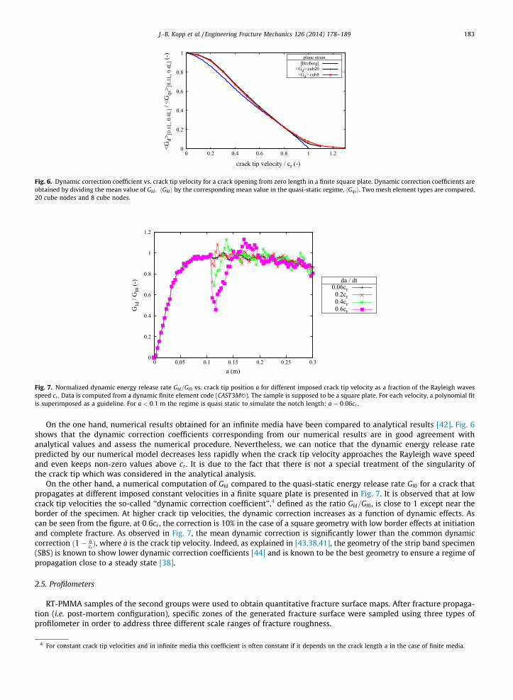
Fig. 7. Normalized dynamic energy release rate GId=GI0 vs. crack tip position a for different imposed crack tip velocity as a fraction of the Rayleigh wavesspeed cr . Data is computed from a dynamic finite element code (CAST3M�). The sample is supposed to be a square plate. For each velocity, a polynomial fitis superimposed as a guideline. For a < 0:1 m the regime is quasi static to simulate the notch length: _a ¼ 0:06cr .

J.-B. Kopp et al. / Engineering Fracture Mechanics 126 (2014) 178–189 183

On the one hand, numerical results obtained for an infinite media have been compared to analytical results [42]. Fig. 6shows that the dynamic correction coefficients corresponding from our numerical results are in good agreement withanalytical values and assess the numerical procedure. Nevertheless, we can notice that the dynamic energy release ratepredicted by our numerical model decreases less rapidly when the crack tip velocity approaches the Rayleigh wave speedand even keeps non-zero values above cr . It is due to the fact that there is not a special treatment of the singularity ofthe crack tip which was considered in the analytical analysis.

On the other hand, a numerical computation of GId compared to the quasi-static energy release rate GI0 for a crack thatpropagates at different imposed constant velocities in a finite square plate is presented in Fig. 7. It is observed that at lowcrack tip velocities the so-called ‘‘dynamic correction coefficient’’,4 defined as the ratio GId=GI0, is close to 1 except near theborder of the specimen. At higher crack tip velocities, the dynamic correction increases as a function of dynamic effects. Ascan be seen from the figure, at 0:6cr , the correction is 10% in the case of a square geometry with low border effects at initiationand complete fracture. As observed in Fig. 7, the mean dynamic correction is significantly lower than the common dynamiccorrection ð1� _a

crÞ, where _a is the crack tip velocity. Indeed, as explained in [43,38,41], the geometry of the strip band specimen

(SBS) is known to show lower dynamic correction coefficients [44] and is known to be the best geometry to ensure a regime ofpropagation close to a steady state [38].

2.5. Profilometers

RT-PMMA samples of the second groups were used to obtain quantitative fracture surface maps. After fracture propaga-tion (i.e. post-mortem configuration), specific zones of the generated fracture surface were sampled using three types ofprofilometer in order to address three different scale ranges of fracture roughness.

4 For constant crack tip velocities and in infinite media this coefficient is often constant if it depends on the crack length a in the case of finite media.

Fig. 8. Laboratory opto-mechanical stylus profilometer: 1-Laser distance meter. 2-Stylus (measurement of z coordinates). 3-Translation stage. 4-Rigidframe between the laser head and rotation axis of the stylus (translation along y axis). 5-Sample (translation along x axis).

184 J.-B. Kopp et al. / Engineering Fracture Mechanics 126 (2014) 178–189

2.5.1. Opto-mechanical profilometer (OMP)Firstly, a prototype of an opto-mechanical stylus profilometer (OMP) at EOST, was used to characterize the fracture sur-

face at the largest scales. The principle of the OMP consists in probing a fracture surface with a mechanical arm carrying astylus (Fig. 8). The stylus is moved horizontally at a constant speed (about 1 mm s�1) and subjected to gravity ensuring thatthe sapphire tip with a diameter of /x ¼ 10 lm keeps in contact with the surface. The vertical movement of the stylus ismonitored by a laser displacement sensor using a triangulation technique with a vertical resolution of 1 lm. Measurementsare discretized along a grid (Nx;Ny) with a mesh (Dx;Dy). The mesh grid is chosen as: Dx ¼ Dy ¼ 10 lm with a resolution of2 lm. This technique is compatible with possible surface transparency which would prevent the use of optical techniques.The present profilometer cumulates optical precision for height measurement and the mechanical description of theair/RT-PMMA interface (no penetration).

2.5.2. Interferometric Optical Microscopy (IOM)Secondly, a Bruker Contour GT-K1 optical microscope has been used. The technique is based on white light confocal inter-

ferometry. It allows the non-contact imaging of surfaces with a vertical sub-nanometer resolution, from nanometer-scaleroughness through millimeter-scale steps. The lateral resolution depends on the size of beam used for the measuring pro-cess. Three beam sizes have been chosen: 88.08 nm, 195.27 nm and 3.64 lm.

2.5.3. Atomic Force Microscopy (AFM)Thirdly, a Bruker Fastscan-A AFM has been used. Imaging is done in ambient conditions with a silicon tip at a scanning

frequency of 1.2 MHz. The size of the tip is approximately 10 nm.

Table 2Features of fracture roughness maps acquired by AFM, OMP and IOM techniques (see text); Br. and S are used respectively for maps sampled in pre-Branchingor Stopping phase zones. Resolution is the size of the sampling square mesh and the probe diameter (P.d.). The area is the size of the sampled zone.

Sample Technique Map name Br. S P. d. (lm) Area (mm2)

JBK1 OMP RT-PMMA1 � 10 25 � 1JBK1 OMP RT-PMMA2 � 10 25 � 1JBK2 OMP RT-PMMA3 � 10 25 � 1JBK2 OMP RT-PMMA4 � 10 30 � 1JBK2 OMP RT-PMMA5 � 10 15 � 1JBK3 OMP RT-PMMA6 � � 10 80 � 1JBK4 OMP RT-PMMA7 � � 10 80 � 1JBK5 OMP RT-PMMA8 � 10 60 � 1JBK6 OMP RT-PMMA9 � � 10 100 � 1.5JBK7 OMP RT-PMMA10 � 10 100 � 1.3ON1 IOM RT-PMMA11 � 3.64 11.4 � 1.4ON1 IOM RT-PMMA11 � 3.64 11.4 � 1.4ON1 IOM RT-PMMA12 � 0.195 0.48 � 0.39ON1 IOM RT-PMMA12 � 0.195 0.48 � 0.39ON1 IOM RT-PMMA13 � 0.088 0.24 � 0.24ON1 IOM RT-PMMA13 � 0.088 0.24 � 0.24ON1 AFM RT-PMMA14 � 0.01 0.025 � 0.025

J.-B. Kopp et al. / Engineering Fracture Mechanics 126 (2014) 178–189 185

2.6. Roughness data

Roughness data recorded by either OMP, IOM or AFM techniques, are topographic maps as (x,y,z) files, along grids withsquare meshes. They were used to estimate the amount of fracture surfaces which was expected to depend on the mesh sizeand probe resolution. The maps’ characteristics are summarized in Table 2.

Fracture maps provide observations of surface roughening during crack propagation. Fig. 9(top) shows the fracture mor-phology before macro-branching. The magnitude of the roughness is at its maximum with large scale topographies. Beforecrack arrest the fracture surface looks rather smooth with sparse irregularities (Fig. 9(bottom)). Of course, with the samplenot being entirely fractured, the latter’s surface is only accessible after cutting into the sample to access the crack arrest zone.A quantitative comparison of the amount of fracture surface between these two situations are compared to the differences indynamic fracture energy GIdc.

3. Results

3.1. Crack tip velocity and hGIdi estimates

During fracture tests, macroscopic crack velocity, which is the measurement of the evolution of the resistance of theconductive layer (Section 2.3), is observed to be quasi constant all along the propagation of each specimen at a given tem-perature (Fig. 10). The reported values are average values over time when the crack tip is within the following specific range[1/4L; 3/4L]. In that range, fluctuations of the crack tip velocity during each experiment is less than the measurement accu-racy error. As shown in Fig. 10, the crack tip velocity is 550 m s�1 � 0:6 � cr with cr � 1025� 15 m s�1. No significant varia-tion in crack speed has been observed either before crack branching or just before crack arrest. In other words, the crack tipvelocity is observed to be the same whether or not branching occurs.

The difference in the initial stress hrzzi leads to fluctuations in dynamic fracture energy GIdc according to Eq. (2) as shownin Fig. 11. It is interesting that at a given crack tip velocity _a, the dynamic fracture energy GIdc can vary up to 300%. To stressout this fluctuation of GIdc; hGIdcimin is computed as the mean of the minima of GIdc over crack tip velocity. Error bars asso-ciated with the average values of hGIdci are estimated as the standard deviation over 8 values for hGIdcimax and 3 values forhGIdcimin which corresponds respectively to crack propagation configurations Br. and S (see Table 1). The mean of the maximaof GIdc at 0:6cr: hGIdcimax is also computed. Table 3 highlights striking variations of GIdc. The ratio hGIdcimax=hGIdcimin suggeststhat GIdc can fluctuate by up to 300%. It is observed that the highest values of GIdc are associated with the roughest surfaceswhile, the lowest values of GIdc are associated with the smoothest surfaces.

Fig. 9. Fracture roughness maps of the fracture surface of sample JBK3 and JBK7 probed by OMP: (top) just before a macro-branching; (bottom) before acrack arrest along an extended dead branch. Horizontal and vertical scales are identical. The arrow indicates the crack propagation direction.

Fig. 10. Crack length aðtÞ vs. time t during two fracture tests: in a case of crack branching (sample SBS2) and in a case of no macroscopic crack branching(sample SBS9). The macroscopic crack speed estimated from the linear fit (dash line) is about 550 m s�1.

Fig. 11. Dynamic fracture energy GIdc averaged over time during each experiment vs. macroscopic crack velocity _a for all 11 experiments (see Table 1).

Table 3Dynamic fracture energy averaged over time (during a simulated experimentation) for the smallest values: hGIdcimin , the highest values: hGIdcimax and themagnitude of the fluctuations (ratio of maximum over the minimum). The smallest values correspond to crack arrest zones and the largest values correspond tobranching zones.

hGIdcimin ðkJ=m2Þ hGIdcimax ðkJ=m2Þ hGIdcimax=hGIdcimin

0:6� 0:1 1:70� 0:2 3:0� 0:2

186 J.-B. Kopp et al. / Engineering Fracture Mechanics 126 (2014) 178–189

3.2. Fracture surface quantifications

A Fortran code has been developed to compute the amount of fracture surface Ar , taking into account the measured frac-ture roughness. From maps (x,y,z), the code introduces a triangulation of the surface by dividing each square mesh sampleinto two adjacent triangles. The total fracture surface Ar is then estimated from the sum of each triangular area over theentire scanned area A0 (see Fig. 12). The same technique can be used for each profilometer type (OMP, IOM, AFM).

The rough fracture surface before macro-branching, (i.e. zone B), ABr , and just before crack arrest (i.e. zone S), AS

r , are com-puted as a function of the amount of projected fracture surface A0, i.e. the size of the scanned area. The results are presentedin Table 4. It has been observed that samples probed with the OMP, i.e. at the coarsest resolution, show a quantity of fracturesurface before a macro-branching which is approximately 10% larger than before crack arrest (AB

r =ASr ¼ 1:10� 0:01). This

estimation is an average over 7 samples with an error bar calculated as the standard deviation over these 7 ratios. The ratiobetween the amount of fracture surface before macro-branching (zone B) and arrest zone (zone S) AB

r =ASr is much larger if a

higher resolution technique (IOM) is used. When the mesh size of the IOM is reduced from 3.64 lm to 0.195 lm on the samefractured zone, the ratio increases up to 210% (see Fig. 13). Interestingly, the ratio AB

r =ASr decreases at a finer resolution

d ¼ 0:088 lm and is even smaller with AFM at the smallest resolution d ¼ 0:01 lm. No error bars are given for IOM and

Fig. 12. Triangulation of a scanned surface. For each 4 node mesh, the real area is approximated by the surface of two adjacent triangles (1 and 2). The totalfracture surface Ar is then the sum of all the triangular areas.

Table 4Estimation of the amount of fracture surfaces as a function of the resolution technique with d the diameter of the probe. Ratios AB

r =A0 and ASr=A0 represent

normalized surfaces by the projected surface A0. The ratio ABr /AS

r is the relative comparison of surface before branching and before arrest.

Technique Sample d (lm) ABr /A0 AS

r /A0 ABr /AS

r

OMP JBK1-7 10 1.11 � 0.01 1.009 � 0.002 1.10 � 0.01IOM ON1 3.64 1.36 1.02 1.33IOM ON1 0.195 2.71 1.29 2.10IOM ON1 0.088 2.34 1.45 1.61AFM ON1 0.01 1.57 1.32 1.20

1

1.2

1.4

1.6

1.8

2

2.2

2.4

-2 -1.5 -1 -0.5 0 0.5 1

ArB

/ A

rS

log10 δ (μm)

Fig. 13. Evolution of the amount of fracture surfaces as a function of the resolution technique with d the experimental measurement step.

J.-B. Kopp et al. / Engineering Fracture Mechanics 126 (2014) 178–189 187

AFM measurements because analysis were performed with only one sample. It is to notice that the ratio ABr =A

Sr for a given

area can be smaller at a higher resolution as the surface is measured with respect to a reference plane A0 or mean plane thatevolves with the resolution. In particular, when the scanned surface is smaller, the mean plane orientation is different.

On a molecular scale, it is expected that all surfaces looks similar. Indeed, self heating induced in the process zone [16,17]combined with the effect of the surface tension acting significantly at this scale, liquids like fibrils form a mirror surface [11].Hence, a transition in surface ratio occurs typically at a lower limit length of 10 nm that corresponds to the fibril scale [45].Equivalently, a transition is expected at the scale of the structure i.e. the size of the specimen. Indeed, at this scale, the devi-ations and bifurcations of the crack path are limited by the possibility of mixed modes (i.e. non-unique mode I). The mode I isseen to be the weakest in many materials. Hence, the transition on a small scale concerns an intrinsic material length whilethe transition on a large scale is related to the sample size.

Table 5Reconstruction at low resolution of the fracture surface from a measurement at higher resolution. The reconstruction is obtained from two techniques:resampling (samp) or convolution (conv) (see text).

Technique Sample name d (lm) ABr /A0 AS

r /A0 ABr /AS

r

IOM ON1 0.195 2.71 1.29 2.09IOM-conv. ON1 10 1.17 1.005 1.16IOM-samp. ON1 10 1.19 1.006 1.18OMP JBK7 10 1.11 1.009 1.10

188 J.-B. Kopp et al. / Engineering Fracture Mechanics 126 (2014) 178–189

Besides, it is found that the amount of created fracture surface depends on the scale at which the surface is scanned. Todirectly check this conclusion, the scale influence on the ratio AB

r =ASr when degrading the sampling resolution was tested for

one specific surface. Only measurements at resolutions larger than d ¼ 0:195 lm were considered. Indeed, for smaller res-olutions, the influence of the sample orientation during measuring was too significant. For instance, a map (ON1), acquiredwith a mesh of 0.195 lm using the IOM instrument, was numerically smoothed to obtain a mesh of 10 lm corresponding tothe OMP technique. Two methods for this reconstruction were used: (1) the resampling method, i.e. keeping only one pointfor every 51 points; (2) the convolution method which consists in computing the convolution of the topography with asphere that mimics a large probe. Table 5 shows that whatever the method used (convolution or sampling), the degradedfracture surface (ON1 with d ¼ 10 lm) is similar, with an error smaller than 8%, to the fracture surface estimated withOMP analysis at the same resolution. Therefore, this test clearly shows that the area of fracture surface is scale dependent.

4. Conclusions

Using a transient dynamic finite element model to analyse experiments and assuming L.E.F.M., the RT-PMMA samplesreveal a loss of unicity of the dynamic fracture energy GIdc for a crack tip velocity of approximately 0:6cr . Indeed, the max-imum value of the fracture energy are up to 3:0� 0:2 times the minimum value. The results suggest that the differences ofGIdc can be associated to the roughness of the fracture surface which introduces a significant difference between the amountof surface created by fracture Ar and the projected area on the mean fracture plane A0. In this article the roughness of a frac-ture surface is obtained from the sampling of post-mortem surfaces. The amount of fracture surface has been quantified froma triangulation of the surface.

By using OMP sampling at a scale of 10 lm, it is shown that the crack creates 10% more surface before a branching zonethan during a crack arrest zone AB

r =ASr ¼ 1:10. Even if a trend is observed at this sampling resolution, the difference in frac-

ture surface is amplified at a smaller scale (i.e. higher resolution) as shown using an interferometric optical profilometer(IOM). Indeed, the ratio AB

r =ASr ¼ 1:10 rises to 1.3 and 2.1 when sampling at 3.64 lm and 0.195 lm, respectively. At an

AFM scale of 0.01 lm, the ratio decreases: ABr =A

Sr ¼ 1:20 which might be interpreted as there being less differences between

ABr and AS

r at nano-metric scale. Indeed, at this scale the orientation of the mean plane during measuring becomes a practicalissue. Significantly changing the orientation of the mean plane has an impact on the magnitude of the measured fractureroughness and subsequently on its effective area. In other words, a significant fluctuation of the area is introduced to thereference area A0. Moreover, at this scale, which corresponds to fibril scale, the same fracture surface roughness is expected.Indeed, with the same micro-structure, all surfaces look similar.

Even if the estimation of the amount of fracture surface is not a simple matter, the present experimental multi-scale anal-ysis suggests that a scale exists at which the maximum ratio between rough and smooth surfaces is encountered. The resultssuggest that the assessment of GIdc at approximately 0:6cr should not be calculated as a function of the amount of projectedfracture surface (A0) on the average fracture plane but, rather, as a function of the amount of fracture surface created, Ar . Forthese kinds of materials, and probably other viscoplastic materials, it seems more adequate to multiply GIdc by Ar=A0 to esti-mate a relevant intrinsic material parameter.

It is interesting to link those results with a statistical approach such as a self-affine geometrical model which describesthe scaling invariance valid for many fracture surfaces [46–51]. This is an on-going work which aims to model the evolutionof the amount of created fracture surface as a function of the sampling scale in order to make large scale measurements, likeOMP measurements, relevant for dynamic fracture energy GIdc assessments.

Acknowledgments

The authors gratefully acknowledge the support of ‘‘Agence Nationale de la Recherche’’ and especially the collaborators of‘‘Carenco’’.

References

[1] Williams JG. Visco-elastic and thermal effects on crack growth in PMMA. Int J Fract 1972;8:393–401.[2] Kobayashi A, Ohtani N, Munemura M. Dynamic stress intensity factors during viscoelastic crack propagation at various strain rates. J Appl Polym Sci

1980;25(12):2789–93.[3] Doll W. Application of an energy balance and an energy method to dynamic crack propagation. Int J Fract 1976;12:595–605.[4] Fineberg J, Gross S, Marder M, Swinney H. Instability in dynamic fracture. Phys Rev Lett 1991;67(4):457–60.

J.-B. Kopp et al. / Engineering Fracture Mechanics 126 (2014) 178–189 189

[5] Rittel D, Maigre H. An investigation of dynamic crack initiation in PMMA. Mech Mater 1996;23(3):229–39.[6] Kopp JB, Lin J, Schmittbuhl J, Fond C. Longitudinal dynamic fracture of polymer pipes. Eur J Environ Civil Engng 2014.[7] Castagnet S, Girault S, Gacougnolle J, Dang P. Cavitation in strained polyvinylidene fluoride: mechanical and X-ray experimental studies. Polymer

2000;41(20):7523–30.[8] Fond C, Schirrer R. Dynamic fracture surface energy and branching instabilities during rapid crack propagation in rubber toughened PMMA. Notes CRAS

Ser IIb 2001;329(3):195–200.[9] Scheibert J, Guerra C, Celarie F, Dalmas D, Bonamy D. Brittle-quasibrittle transition in dynamic fracture: an energetic signature. Phys Rev Lett 2010;104.

045501-1–045501-4.[10] Sharon E, Fineberg J. Confirming the continuum theory of dynamic brittle fracture for fast cracks. Nature 1999;397:333–5.[11] Fond C, Schirrer R. Influence of crack speed on fracture energy in amorphous and rubber toughened amorphous polymers. Plast Rubber Compos

2001;30(3):116–24.[12] Morel S, Schmittbuhl J, Bouchaud E, Valentin G. Scaling of crack surfaces and implications for fracture mechanics. Phys Rev Lett 2000;85:1678–81.[13] Lovell PA, Sherratt MM, Young RJ. Mechanical Properties and deformation micromechanics of rubber-toughened acrylic polymers. In: Toughened

plastics II. Advances in chemistry, vol. 252. American Chemical Society; 1996. p. 211–32 [chapter 15], ISBN13: 9780841231511, eISBN:9780841224377.

[14] Fond C. Cavitation criterion for rubber materials: a review of void-growth models. J Polym Sci Part B: Polym Phys 2001;39(17):2081–96.[15] Fond C, Schirrer R. Renforcement des polymères – mécanismes et modélisations de la cavitation. In: Physique des polymères à l’état solide; vol. 17;

2006. p. 167–208 [chapter 6].[16] Anderson TL. Fundamentals and applications. 3rd ed. Taylor and Francis Group; 2005.[17] Bradley W, Cantwell W, Kausch H. Viscoelastic creep crack growth: a review of fracture mechanical analyses. Mech Time-Depend Mater

1997;1(3):241–68.[18] Bohme W, Kalthoff JF. On the quantification of dynamic in impact loading and the practical application for kid-determination. J Phys Colloques

1985;46. C5-213–C5-218.[19] Kalthoff JF. On the measurement of dynamic fracture toughnesses? a review of recent work. Int J Fract 1985;27:277–98.[20] Krishnaswamy S, Tippur HV, Rosakis AJ. Measurement of transient crack-tip deformation fields using the method of coherent gradient sensing. J Mech

Phys Solids 1992;40(2):339–72.[21] Rosakis A. Two optical techniques sensitive to gradients of optical path difference: the method of caustics and the Coherent Gradient Sensor (CGS).

Epstein, JS; 1993.[22] Tippur HV, Krishnaswamy S, Rosakis AJ. Optical mapping of crack tip deformations using the methods of transmission and reflection coherent gradient

sensing: a study of crack tip K-dominance. Int J Fract 1991;52:91–117.[23] Takahashi K, Arakawa K. Dependence of crack acceleration on the dynamic stress-intensity factor in polymers. Exp Mech 1987;27(2):195–9.[24] Ivankovic A, Demirdzic I, Williams J, Leevers P. Application of the finite volume method to the analysis of dynamic fracture problems. Int J Fract

1994;66(4):357–71.[25] Ferrer J, Fond C, Arakawa K, Takahashi K, Beguelin P, Kausch H. The influence of crack acceleration on the dynamic stress intensity factor during rapid

crack propagation. Int J Fract 1997;87(3):L77–82.[26] Fond C, Schirrer R. Fracture surface energy measurement at high crack speed using a strip specimen: application to rubber toughened PMMA. Journal

de Physique IV 1997;7. C3-969–C3-974.[27] Fond C, Schirrer R. Dynamic fracture surface energy values and branching instabilities during rapid crack propagation in rubber toughened PMMA. CR

Acad Sci Ser IIb: Mec 2001;329(3):195–200.[28] Bucknall CB, Schmith RR. Stress-whitening in high-impact polystyrenes. Polymer 1965;6:437–46.[29] Keskkula H, Schwarz M, Paul DR. Examination of failure in rubber toughened polystyrene. Polymer 1986;27(2):211–6.[30] Dagli G, Argon A, Cohen R. Particle-size effect in craze plasticity of high-impact polystyrene. Polymer 1995;36(11):2173–80.[31] Borggreve R, Gaymans R, Schuijer J, Ingen Housz J. Brittle-tough transition in nylon-rubber blends: effect of rubber concentration and particle size.

Polymer 1987;28(9):1489–96.[32] Borggreve R, Gaymans R, Schuijer J. Impact behaviour of nylon-rubber blends: 5. Influence of the mechanical properties of the elastomer. Polymer

1989;30(1):71–7.[33] Schmittbuhl J, Schmitt F, Scholz C. Scaling invariance of crack surfaces. J Geophys Res 1995;100(B4):5953–73.[34] Deumié C, Richier R, Dumas P, Amra C. Multiscale roughness in optical multilayers: atomic force microscopy and light scattering. Appl Opt

1996;35(28):5583–94.[35] Candela T, Renard F, Klinger Y, Mair K, Schmittbuhl J, Brodsky E. Roughness of fault surfaces over nine decades of length scales. J Geophys Res B: Solid

Earth 2012;117(8).[36] He C, Donald A. Morphology of a deformed rubber toughened poly(methyl methacrylate) film under tensile strain. J Mater Sci 1997;32:5661–7.[37] Schmittbuhl J, Chambon G, Hansen A, Bouchon M. Are stress distributions along faults the signature of asperity squeeze. Geophys Res Lett 2007;33:L-

13307.[38] Nilsson F. Dynamic stress-intensity factors for finite strip problems. Int J Fract 1972;8:403–11.[39] Yoffe EH. The moving griffith crack. Philos Mag 1951;42:739–50.[40] Guo C, Sun C. Dynamic mode-I crack-propagation in a carbon/epoxy composite. Compos Sci Technol 1998;58(9):1405–10.[41] Fond C. Endommagement des polymères choc: modélisations micromécaniques et comportements à la rupture. Habilitation à diriger des recherches

en mécanique des solides; Université Louis Pasteur de Strasbourg; 2000.[42] Broberg KB. The propagation of a brittle crack. Arkiv Fysik 1960;18:159.[43] Popelar C, Atkinson C. Dynamic crack propagation in a viscoelastic strip. J Mech Phys Solids 1980;28(2):79–93.[44] Freund L. Crack propagation in an elastic solid subjected to general loading-i. Constant rate of extension. J Mech Phys Solids 1972;20(3):129–40.[45] Halary J, Lauprêtre F, Monnerie L. Mécanique des matériaux polymères. Échelles (Paris); Belin; 2008. ISBN 9782701145914.[46] Schmittbuhl J, Gentier S, Roux S. Field measurements of the roughness of fault surfaces. Geophys Res Lett 1993;20(8):639–41.[47] Meakin P. Fractals: Scaling and growth far from equilibrium. Cambridge university press; 1998.[48] Candela T, Renard F, Bouchon M, Brouste A, Marsan D, Schmittbuhl J, et al. Characterization of fault roughness at various scales: implications of three-

dimensional high resolution topography measurements. Pure Appl Geophy 2009:1817–51.[49] Simonsen I, Hansen A, Nes OM. Determination of the hurst exponent by use of wavelet transforms. Phys Rev E 1998;58:2779–87.[50] Mandelbrot B, Passoja D, Paulay AJ. Fractal character of fracture surfaces of metals. Nature 1984;308:721–2.[51] Maloy K, Hansen A, Hinrichsen E, Roux S. Experimental measurements of the roughness of brittle cracks. Phys Rev Lett 1992;68:213–5.