engineering fracture mechanics - materials technology multiscale modelling of heterogeneous material...

Engineering Fracture Mechanics 76 (2009) 793–812

Contents lists available at ScienceDirect

Engineering Fracture Mechanics

journal homepage: www.elsevier .com/locate /engfracmech

Computational multiscale modelling of heterogeneous material layers

C.B. Hirschberger a,d,*,1, S. Ricker a,2, P. Steinmann b, N. Sukumar c

a Department of Mechanical and Process Engineering, University of Kaiserslautern, P.O. Box 3049, 67653 Kaiserslautern, Germanyb Department of Mechanical Engineering, University of Erlangen–Nuremberg, Egerlandstraße 5, 91058 Erlangen, Germanyc Department of Civil and Environmental Engineering, University of California at Davis, One Shields Avenue, Davis, CA 95616, USAd Department of Mechanical Engineering, Eindhoven University of Technology, P.O. Box 513, 5600 MB Eindhoven, The Netherlands

a r t i c l e i n f o

Article history:Received 28 February 2008Received in revised form 29 July 2008Accepted 26 October 2008Available online 27 November 2008

Keywords:Cohesive interfacesMultiscale modellingComputational homogenizationFinite-element analysis

0013-7944/$ - see front matter � 2008 Elsevier Ltddoi:10.1016/j.engfracmech.2008.10.018

* Corresponding author. Present address: DepartmThe Netherlands. Tel.: +31 402472245; fax: +31 402

E-mail addresses: [email protected] ([email protected] (N. Sukumar).

1 Grant sponsor: Deutsche Forschungsgemeinschaf2 Grant sponsor: Deutsche Forschungsgemeinschaf

a b s t r a c t

A computational homogenization procedure for a material layer that possesses an under-lying heterogeneous microstructure is introduced within the framework of finite deforma-tions. The macroscopic material properties of the material layer are obtained frommultiscale considerations. At the macro level, the layer is resolved as a cohesive interfacesituated within a continuum, and its underlying microstructure along the interface is trea-ted as a continuous representative volume element of given height. The scales are linkedvia homogenization with customized hybrid boundary conditions on this representativevolume element, which account for the deformation modes along the interface. A nestednumerical solution scheme is adopted to link the macro and micro scales. Numerical exam-ples successfully display the capability of the proposed approach to solve macroscopicboundary value problems with an evaluation of the constitutive properties of the materiallayer based on its micro-constitution.

� 2008 Elsevier Ltd. All rights reserved.

1. Introduction

Material layers that transmit cohesive tractions occur in several engineering disciplines. Solder connections, adhesivebonding layers, laminated composite structures, building materials such as masonry, as well as geomaterials are some nota-ble examples. Two are illustrated in Fig. 1. In most cases, the material in the connecting layer is significantly weaker than thesurrounding bulk material and therefore the deformation will be strongly confined to this layer. If the material layer is com-posed of a heterogeneous microstructure, the geometric and material properties of that will crucially govern the globalbehaviour. Such heterogeneities can for instance appear as voids, micro cracks, or inclusions, and can be found in fibre-rein-forced materials (e.g., metal–polymer matrix, concrete), or in natural materials (e.g., geological conglomerates). Homogeni-zation approaches as pioneered by Hill [4,5] provide an appropriate framework to relate the mechanical behaviour withinthe different spatial scales of observation. The key issue of the current contribution is to account for this microstructureof the material layer in an appropriate way. Beyond existing approaches, which are achieved for instance by asymptotichomogenization [15,16], we particularly aim to propose a computational multiscale framework that is suitable for nonlinearmultiscale finite-element simulations in the spirit of FE.2

Within a multiscale consideration, on the macro scale the material layer is treated as a cohesive interface situated withina continuum. The governing quantities in this cohesive interface, i.e. the displacement jump (or rather separation) and the

. All rights reserved.

ent of Mechanical Engineering, Eindhoven University of Technology, P.O. Box 513, 5600 MB Eindhoven,447355.Hirschberger), [email protected] (S. Ricker), [email protected] (P. Steinmann),

t (DFG) via the International Research Training Group 1131.t (DFG) via the Research Training Group 814.

mailto:[email protected]




http://www.sciencedirect.com/science/journal/00137944

http://www.elsevier.com/locate/engfracmech

Fig. 1. (a) Adhesive bonding of two solid substrates with a polymeric glue: circular uni-axial tension specimen with incompletely cured polyurethane layer(courtesy of Gunnar Possart). (b) Material layer within geological bulk material of different properties.

794 C.B. Hirschberger et al. / Engineering Fracture Mechanics 76 (2009) 793–812

cohesive tractions, are related based on the underlying microstructure rather than employing an a priori constitutiveassumption, coined as a cohesive traction–separation law. On the micro scale, representative volume elements (RVE) alongthe material layer advocate the heterogeneous microstructure, as illustrated in Fig. 2. Their height is directly given by thethickness of the material layer. For the concept of representative volume elements the reader is for instance referred to Refs.[5,28]. The micro–macro transition between the RVE and the interface is achieved based upon the averaging of the governingkinematic, stress and energetic quantities over the respective underlying RVE. The boundary conditions stemming from thecohesive interface at the macro level imposed on the RVE must be chosen consistently – on the one hand, they need to fulfilthe Hill condition [5], which ensures the equivalence of the macro and the micro response, whereas on the other hand, theboundary conditions shall account for the interface geometry and capture the occurring mixed-mode (shear and tension)deformation modes.

The homogenization approach is numerically implemented within a computational homogenization along the lines ofRefs. [9–11,20–22,24,25]. Within a geometrically nonlinear finite-element framework, we straightforwardly model thematerial layer by means of cohesive interface elements situated between the adjacent bulk finite elements. With these ele-ments, the finite-element formulation which can be found in Refs. [1,18,23,29,30,34,35,37], the constitutive relation consistsby a cohesive traction–separation law, which has traditionally been treated by a priori assumptions, as they were proposedby Xu and Needleman [27,38]. Instead of using such constitutive assumption, we obtain the material response from compu-

Fig. 2. Heterogeneous material layer, which is shown over-sized for the sake of visibility, situated within a macro bulk material with sketches of RVEs thatare locally periodic, but may vary along the material layer.

C.B. Hirschberger et al. / Engineering Fracture Mechanics 76 (2009) 793–812 795

tational homogenization. To this end, the solution of a micro scale boundary value problem is invoked at each integrationpoint of each interface elements. Thereby upon application of customized hybrid boundary conditions stemming from theinterface, the macroscopic constitutive behaviour is extracted at the RVE boundaries towards the bulk. The representativevolume element is modelled as a nonlinear finite-element boundary value problem, which is subjected to the deformationinduced by the interface element on the macro scale. The macroscopic traction and the constitutive tangent operator for aNewton–Raphson solution scheme are extracted from the micro problem. In this way, a fully nested iterative multiscalesolution for a bulk including a material layer accounting for the micro-heterogeneous properties of the latter isaccomplished.

The current paper extends the multiscale approach of Matous et al. [17] to the general case of finite deformations. Beyondboth the latter contribution and that of Larsson and Zhang [14], not only the cohesive behaviour of the microscopically het-erogeneous material layer shall be considered, but rather we are interested in solving macroscopic boundary value problemsinvolving this material layer. To this end, emphasis is placed on a multiscale framework, that utilizes computational homog-enization. If the intrinsic microstructure is negligibly small such that no size effects occur, as is the case in the current paper,we restrict ourselves to a classical (Boltzmann) continuum within the representative volume element. In contrast, if the sizeeffect of the intrinsic microstructure is significant, the microstructure can be modelled as a micromorphic continuum, whichis pursued in Ref. [7].

1.1. Outline and notation

The remainder of the paper is structured as follows: In Section 2, we present the continuum mechanics framework on themacro scale with the material layer treated as a cohesive interface. In Section 3, the governing equations for the represen-tative volume element that represents the underlying microstructure, are presented. Once both the macro and the micro le-vel descriptions are present, the micro–macro transition based on the homogenization of the decisive micro quantities isexamined in Section 4. Section 5 provides the numerical framework of the computational homogenization. Numerical exam-ples in Section 6 exhibit the main features of the proposed approach, and finally some concluding remarks are mentioned inSection 7. For the sake of distinction and clarity, the quantities on the macro scale are denoted by an over-bar �ð�Þ, whereas allother quantities refer to the micro scale.

2. Material layer represented by an interface at the macro level

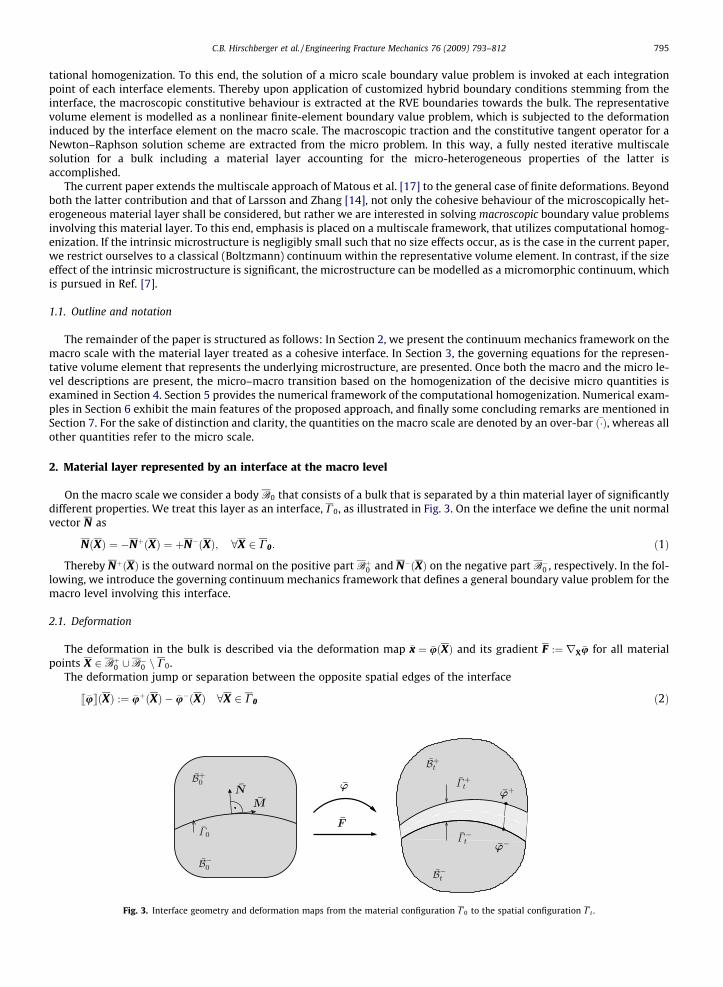
On the macro scale we consider a body B0 that consists of a bulk that is separated by a thin material layer of significantlydifferent properties. We treat this layer as an interface, C0, as illustrated in Fig. 3. On the interface we define the unit normalvector N as

NðXÞ ¼ �NþðXÞ ¼ þN�ðXÞ; 8X 2 C0: ð1Þ

Thereby NþðXÞ is the outward normal on the positive part Bþ0 and N�ðXÞ on the negative part B�0 , respectively. In the fol-lowing, we introduce the governing continuum mechanics framework that defines a general boundary value problem for themacro level involving this interface.

2.1. Deformation

The deformation in the bulk is described via the deformation map �x ¼ �uðXÞ and its gradient F :¼ r�X �u for all materialpoints X 2 Bþ0 [B�0 n C0.

The deformation jump or separation between the opposite spatial edges of the interface

s�utðXÞ :¼ �uþðXÞ � �u�ðXÞ 8X 2 C0 ð2Þ

Fig. 3. Interface geometry and deformation maps from the material configuration C0 to the spatial configuration Ct .


acts as the primary deformation quantity of the interface. The vectorial representation at this point incorporates a loss ofinformation compared to the full deformation tensor. Nevertheless, for the considered material layer this assumption is fullysufficient, since its initial height h0 is much smaller than the total extension of the bulk.

2.2. Equilibrium

For the material body B0 to be in equilibrium the balance of momentum for the bulk B0 n C0 and the equilibrium relationsfor the cohesive interface C0 must be fulfilled. The balance of momentum for the bulk reads

DivP ¼ �b0 in B0 n C0; ð3Þ

in terms of the Piola stress P. The corresponding Neumann and Dirichlet boundary conditions prescribe the spatial traction �t0

with respect to material reference or the deformation map �u on the respective part of the boundary:

P � N ¼: �t pre0 on @BP

0; �u ¼: �upre on @Bu0 : ð4Þ

Across the interface, cohesive tractions are transmitted. The additional equilibrium condition concerning the interface

�tþ0 þ �t�0 ¼ 0; ð5Þ

together with the Cauchy theorem entails a relation for the jump of the Piola stress, sPt, and for its average fPg across thediscontinuity:

sPt � N ¼ 0; fPg � N ¼ �t0 on �C0: ð6Þ

The weak formulation of the balance relations Eqs. (3)–(6) renders the virtual work statement, which requires the sum ofthe internal contributions of both the bulk and the interface to equal the external virtual work:

ZB0nC0

P : dF dV þZ

C0

�t0 � sd�utdA ¼ZB0

�b0 � d�udV þZ@BP

0

�tpre0 � d�udA: ð7Þ

The relation between the stress and the deformation measures is supplied via a constitutive relation.

2.3. Constitutive framework

For the surrounding bulk, we avail ourselves of a hyperelastic constitutive formulation which is stated a priori, for in-stance a neo-Hooke ansatz. Thus the Piola stress is evaluated from the stored-energy density as P ¼ DFW0.

The traction �t0 transmitted across the cohesive interface is energetically conjugate to the separation s�ut in a hyperelasticformat. Within an entirely reversible isothermal constitutive framework, it is a function of the interface separation, i.e.�t0ðs�utÞ. Our objective is to find such a relation based on the underlying microstructure using a multiscale approach. Partic-ularly, in the context of a numerical finite-element simulation utilizing a Newton–Raphson procedure, we are moreoverinterested in the tangent operator A in an incremental traction–separation law

d�t0 ¼ A � sd�ut; A :¼ Ds�ut�t0: ð8Þ

Towards a multiscale framework we will next present a formulation for the underlying microstructure and thereafterbridge the two scales by means of homogenization.

3. Representative volume element at the micro level

Within the proposed multiscale approach, we now consider the modelling of the underlying heterogeneous microstruc-ture. As was illustrated in Fig. 2, representative volume elements are used to model statistically representative portions ofthe material layer. To match them with the interface geometry, we align these volume elements with the interfacial planeand limit its dimension out of plane by the initial height h0 of the material layer. Thereby the dimension of the RVE in planemust be chosen sufficiently large to make the element representative, yet small enough compared to the in plane dimensionof the layer to exclude boundary effects. In the two-dimensional setting pursued here, such element has an initial width w0

and thus a material volume (or rather area) of V0 ¼ w0h0.Any appropriate mechanical framework could be employed on the RVE level, such as a continuum (either in a standard, a

higher-order or a higher-grade formulation), discrete particles to account for granular media, molecular dynamics, or atom-istics, just to mention a few. However, in this article we restrict ourselves to a standard (or rather Boltzmann) continuum,whereas a further extension to a micromorphic RVE accounting for size effects induced by a significant intrinsic microstruc-ture can be found in Ref. [7]. In order to clarify the notation at the micro level, we will in the following briefly review thegoverning equations stating a boundary value problem on the RVE. Based upon this geometrically nonlinear framework,the connections with the macro problem will be treated in Section 4.

Fig. 4. RVE geometry and deformation maps from the material configuration B0 to the spatial configuration Bt .


3.1. Deformation

The finite deformation, also illustrated in Fig. 4, is described through the deformation map u and the deformation gradient F:

x ¼ uðXÞ; FðXÞ :¼ rXuðXÞ 8X 2 @B0: ð9Þ

The placement X can be chosen with respect to any basis; however for practical reasons corresponding to the micro–macro transition, the origin shall be placed in the geometric centre of the RVE.

3.2. Equilibrium

The representative volume element is in equilibrium if the balance of momentum for the static case

DivP ¼ 0 in B0; ð10Þ

is fulfilled under the supplied Neumann and Dirichlet boundary conditions:

P � N ¼: tpre0 on @BP

0; u ¼: upre on @Bu0 : ð11Þ

Thereby at a particular part of the boundary, either the spatial traction t0 ¼ P � N or the deformation u may be prescribed,with @BP

0 \ @Bu0 ¼ ;.

At the micro level, the influence of the body force is neglected, as suggested for instance by [21]. This choice proves con-venient in view of the homogenization, which utilizes only quantities on the RVE boundary. With this assumption, the cor-responding virtual work statement at the micro level reads:
Z
B0

P : dFdV ¼Z@B0

t0 � dudA: ð12Þ

3.3. Constitutive framework

Any appropriate constitutive formulation could be incorporated. However, for the sake of clarity of exposition, we availourselves of a straightforward hyperelastic format for the stored-energy density.

3.4. Boundary value problem

The representative volume element is subjected to boundary conditions that stem from the interfacial traction and sep-aration at the macro level. The necessary relations connecting the two scales consistently with respect to the geometry of thematerial layer will be addressed in the following section.

4. Micro–macro transition

The proposed homogenization approach is based on the averaging of the governing quantities over the volume of the RVEas proposed by Hill [4,5]. First, we recall the volume averages of the deformation gradient, the stress, and the virtual workover the RVE, as they are well-known from the literature. Then, these RVE averages are related to the governing quantities inthe interface. Boundary conditions on the RVE finalize a consistent scale transition.

4.1. Averages of micro quantities over the RVE

The average of the deformation gradient F over the volume of the RVE is given as

hFi ¼ 1V0

ZB0

FdV ¼ 1V0

Z@B0

u� NdA: ð13Þ


The volume average of the Piola stress P in the RVE

hPi ¼ 1V0

ZB0

PdV ¼ 1V0

Z@B0

t0 � XdA; ð14Þ

is required in view of the macroscopic traction vector �t0 in the interface given in Eq. (6)2. Finally, based on Eq. (12) the aver-age of the virtual work in the RVE reads

hP : dFi ¼ 1V0

ZB0

P : dFdV ¼ 1V0

Z@B0

du � t0dA: ð15Þ

Thereby, as already mentioned in Section 3.1, we assume without loss of generality that the origin of the coordinate sys-tem is placed in the geometric centre of the RVE. The following canonical auxiliary relations [2,21]

F ¼ Divðu� IÞ; Pt ¼ DivðX � PÞ; P : F ¼ Divðu � PÞ; ð16Þ

are utilized to convert the averaging theorems from volume to surface integrals. For the latter two conversions, the equilib-rium in omission of body forces was used, as for instance also documented in Refs. [10].

4.2. Micro–macro transition

In order to accomplish a consistent transition between the micro and the macro level, the averaged RVE quantities need tobe related to the interface quantities. Therefore, the deformation, the traction as well as the virtual energy need to be equiv-alent on both scales.

4.2.1. DeformationUpon the consideration of the initial height h0 of the material layer, the averaged deformation gradient Eq. (13) is linked

to the interface kinematics on the macro level as follows: Since the governing kinematic quantity on the RVE level is given bythe homogenized deformation gradient, which is tensor of second order, it is desirable to find a second-order tensor to rep-resent the macro interface deformation as well. Therefore we avail ourselves of a deformation tensor, which was first pro-posed in the context of localized plasticity, (see, for instance Refs. [12,13,31,32]):

F :¼ I þ 1h0

s�ut� N: ð17Þ

Instead of an artificial scaling parameter, which in those approaches is used to achieve regularization, here indeed theinitial height h0 enters this deformation tensor. Clearly, this measure resolves the information given by the macro separationas follows:

F ¼M �M þ 1h0

s�ut �M� �

M � N þ 1þ 1h0

s�ut � N� �

N � N; ð18Þ

or translated into a straightforward matrix notation with respect to the orthonormal basis ðM;NÞ:

Fe1 s �uMt=h0

0 1þ s�uNt=h0

" #: ð19Þ

With this macro assumption at hand, we can relate the macro deformation to the RVE average deformation gradient as

I þ 1h0

s�ut� N � hFi: ð20Þ

Although it obeys the restriction that M � F �M ¼ 1, it involves all the information that is contained in the vectorial rep-resentation of the interface separation s�ut. This assumption yields a somewhat rigorous restriction on the deformation of theRVE, as we will examine later on.

4.2.2. TractionThe traction �t0 in the interface is related to the averaged Piola stress Eq. (14) in the underlying RVE based on the Cauchy

theorem Eq. (6)2:

�t0 � hPi � N ð21Þ

assuming the average RVE Piola stress to be equivalent to the average across the interface of the Piola stress on the macroscale hPi � fPg.

4.2.3. Virtual workThe Hill condition requires the virtual work performed in the interface to be equivalent to the average of the virtual work

performed within the representative volume element. The RVE virtual work density, P : dF , acts within a continuum element


dV and the interface virtual work density is referred to a surface element dA. Due to their different dimension, the average ofthe virtual work in the underlying RVE, Eq. (15), needs to be scaled by the height h0 of the material layer and we obtain

�t0 � sd�ut � h0hP : dFi: ð22Þ

With the particular equivalences of the interfacial separation Eq. (17) and traction Eq. (21), with this condition the usualrequirement in the form

hPi : hdFi � hP : dFi ð23Þ

is retrieved. In this form the Hill condition requires the average of the virtual work performed in the RVE to equal the virtualwork performed by the respective averages of the deformation gradient, Eq. (13), and the stress, Eq. (14), and was thus alsoreferred to as the macro-homogeneity condition [2].

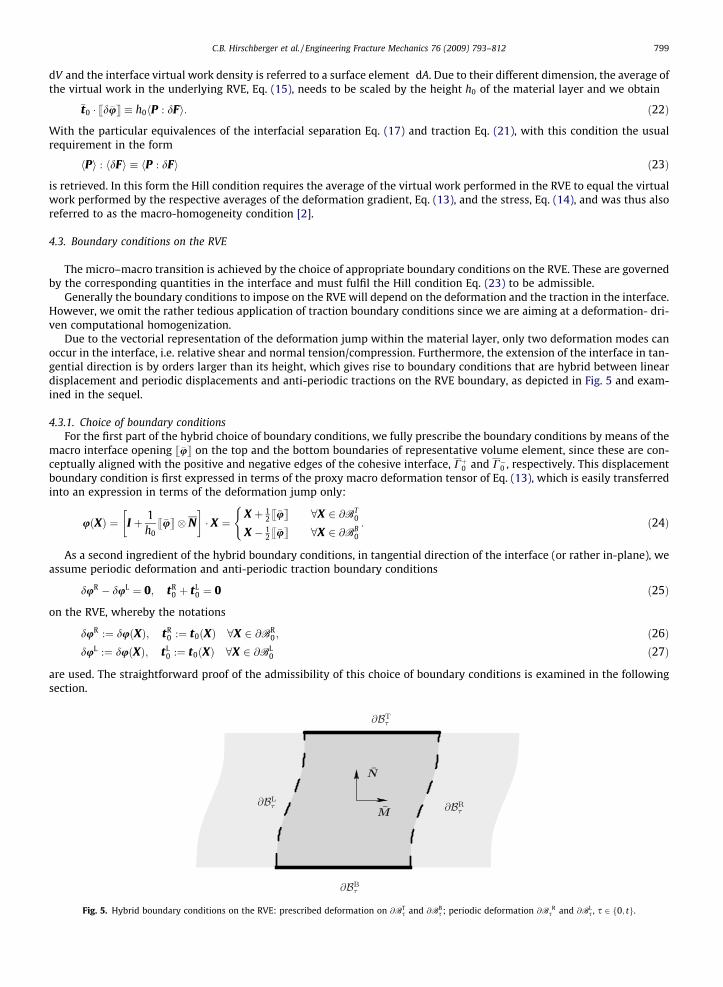
4.3. Boundary conditions on the RVE

The micro–macro transition is achieved by the choice of appropriate boundary conditions on the RVE. These are governedby the corresponding quantities in the interface and must fulfil the Hill condition Eq. (23) to be admissible.

Generally the boundary conditions to impose on the RVE will depend on the deformation and the traction in the interface.However, we omit the rather tedious application of traction boundary conditions since we are aiming at a deformation- dri-ven computational homogenization.

Due to the vectorial representation of the deformation jump within the material layer, only two deformation modes canoccur in the interface, i.e. relative shear and normal tension/compression. Furthermore, the extension of the interface in tan-gential direction is by orders larger than its height, which gives rise to boundary conditions that are hybrid between lineardisplacement and periodic displacements and anti-periodic tractions on the RVE boundary, as depicted in Fig. 5 and exam-ined in the sequel.

4.3.1. Choice of boundary conditionsFor the first part of the hybrid choice of boundary conditions, we fully prescribe the boundary conditions by means of the

macro interface opening s�ut on the top and the bottom boundaries of representative volume element, since these are con-ceptually aligned with the positive and negative edges of the cohesive interface, Cþ0 and C�0 , respectively. This displacementboundary condition is first expressed in terms of the proxy macro deformation tensor of Eq. (13), which is easily transferredinto an expression in terms of the deformation jump only:

uðXÞ ¼ I þ 1h0

s�ut� N� �

� X ¼X þ 1

2 s�ut 8X 2 @BT0

X � 12 s�ut 8X 2 @BB

0

(: ð24Þ

As a second ingredient of the hybrid boundary conditions, in tangential direction of the interface (or rather in-plane), weassume periodic deformation and anti-periodic traction boundary conditions

duR � duL ¼ 0; tR0 þ tL

0 ¼ 0 ð25Þ

on the RVE, whereby the notations

duR :¼ duðXÞ; tR0 :¼ t0ðXÞ 8X 2 @BR

0 ; ð26ÞduL :¼ duðXÞ; tL

0 :¼ t0ðXÞ 8X 2 @BL0 ð27Þ

are used. The straightforward proof of the admissibility of this choice of boundary conditions is examined in the followingsection.

Fig. 5. Hybrid boundary conditions on the RVE: prescribed deformation on @BTs and @BB

s ; periodic deformation @B Rs and @BL

s , s 2 f0; tg.


The vectorial representation of both separation and traction in the interface restricts the deformation to two deformationmodes: shearing tangential to the interface plane and tension out of the interface plane, which is also reflected by the defor-mation measure in Eq. (13). Therefore, with this model, it is not possible to account for in-plane tension within the RVE.However, the macro level does not sense this restriction and the lateral contraction along the interface is entirely controlledby the surrounding bulk in a natural manner.

4.3.2. Admissibility of hybrid boundary conditionsTo show that this choice of boundary condition fulfil the Hill condition (Eq. (23)), the relation hPi : hdFi ¼ hP : hdFii is

used. The Hill condition holds if the following identity is fulfilled:

h0hP : dFi � h0hP : hdFii ¼: 0: ð28Þ

For the proposed hybrid boundary conditions, this relation is both shown to be fulfilled for the prescribed deformation onthe top and the bottom boundary of the RVE and for the periodic in-plane deformation.

To this end, the relation is transformed to the following:

h0hP : dFi � h0hP : hdFii ¼ 1w0

Z@B0

t0 � ½du� hdFi � X�dA0: ð29Þ

For the prescribed displacement (Eq. (24)) the term in brackets directly vanishes and thus the entire integral becomes zero.In a second step, the periodic boundary conditions (Eq. (25)) in-plane are shown to be admissible by regarding (Eq. (29)).

Since for a macro deformation (Eq. (24)) affinely imposed on the RVE, the term hdFi � X is periodic to begin with, thus thefluctuation term du� hdFi � X proves periodic as well. Consequently the integral

1w0

Z@BL

0

t0 � ½du� hdFi � X�dAþ 1w0

Z@BR

0

t0 � ½du� hdFi � X�dA ¼ 0 ð30Þ

vanishes over opposite periodic boundaries if the traction t0 is anti-periodic, which itself follows from equilibrium. Due totheir periodicity, the sum of the integrals over the opposite edges on the left and the right side BL

0 and B R0 , respectively, van-

ishes as described.To gather all contributions of the hybrid boundary conditions, we build the sum of the particular parts of Eqs. (29) and

(30)

h0hP : dFi � h0hP : hdFii ¼ 1w0

Z@B0

t0 � ½du� hdFi � X�dA

¼ 1w0

Z@BT

0

t0 � ½du� hdFi � X� dAþ 1w0

Z@BB

0

t0 � ½du� hdFi � X�dA

þ 1w0

Z@BL

0

t0 � ½du� hdFi � X�dAþ 1w0

Z@BR

0

t0 � ½du� hdFi � X� dA ¼ 0: ð31Þ

This is then zero as well, because each of the first terms is zero and due to the anti-periodicity the sum of the latter two iszero. Thus the proposed hybrid boundary conditions are admissible.

5. Computational homogenization

The homogenization framework of the preceding section is now transferred to a computational homogenization schemein the FE2 spirit of Refs. [3,9,11,25]. This consists of a nested solution scheme [11] involving both the macro- and the micro-level boundary value problems, which are solved iteratively by means of the nonlinear finite-element method.

Situated between the bulk elements, interface elements, as they were introduced in Ref. [1], represent the material layeron the macro scale. The constitutive behaviour of the bulk is assumed a priori, for which a constitutive routine is provided.Contrary, the constitutive behaviour or rather the traction–separation relation Eq. (8) of the interface element is obtainedfrom the underlying microstructure. For this purpose, at each integration point of each interface element, the traction vector�t0 and the tangent operator A are evaluated by means of a computational homogenization of the underlying micro-proper-ties in the RVE based on the macro kinematics as illustrated in Fig. 6.

5.1. Nested solution procedure

The nested multiscale solution, which involves one macro boundary value problem and as many RVE boundary valueproblems as integration points in the macroscopic interface elements of Fig. 6, is in particular achieved as follows.

The macro specimen Bh0 is discretized with bulk finite elements in Bh

0, while cohesive interface elements represent thematerial layer on Ch

0. The formulations of these interface element are well-established and for instance are described in Refs.[23,30,34,35]. Assigned to each macro integration point of each interface element, the corresponding RVE is discretized witha finite-element mesh in Bh

0. In order to handle the in-plane periodicity being part of the hybrid boundary conditions, this

Fig. 6. Computational homogenization between the interface integration point (IP) of the interface element on Ce0 at the macro scale and the underlying

discretized representative volume element Bh0 with boundary @Bh

0.


RVE mesh is subject to the restriction that the left and the right boundary, @BhL0 and @BhR

0 , respectively, have equal arrange-ment. In order to achieve a geometrically nonlinear multiscale solution, at each macroscopic iteration step within a Newton–Raphson algorithm, in each integration point of each interface element the nonlinear systems of the RVEs are solvediteratively subject to the current macro deformation jump, as depicted in the schematic flow chart of Fig. 7, see also Ref.[8]. In particular at each integration point of each interface element on Ch

0 the macro separation s�ut is evaluated iteratively,being zero initially. Its increments deliver the boundary conditions to the RVE finite-element mesh, see Eq. (24). During eachmacro iteration step, the nonlinear micro systems are solved subject to these incremental boundary conditions. When equi-librium is obtained at the RVE level, both the homogenized macroscopic tangent operator A and the macroscopic tractionvector �t0 of Eq. (8) at the respective integration point along the interface are computed from this solution. Precisely, the con-tributions of the stiffness matrix and the residual vector at the RVE boundary are extracted to this end. With the constitutivemacro quantities at hand, the macro system is solved iteratively until a global solution for the current load step is obtained.In case the interface coordinate system does not coincide with the global coordinate system, the components of the separa-tion vector in tangential and normal direction are transferred to the RVE.

5.1.1. Nonlinear system at the macro levelAt the macro level, the global residual must vanish for all degrees of freedom �uI . Based on the weak form Eq. (7), it is

obtained from an assembly of the contributions of all the bulk and all the interface elements as

RI ¼ A�nel

�e¼1

Z e

B0

P � r�XN �uI dV þ A

�niel

ie¼1

ZCe

0

�t0 � Ns�ut

I dA� �fextI ¼

: 0: ð32Þ

Herein the shape functions N �uI act in the bulk and Ns�ut

I within the interface element. The external force vector at themacro level in general contains both external traction and body forces acting on the bulk surface and volume, respectively:

�fextI ¼ A

�nel

�e¼1

ZBe

0

�b0�N �u

I dV þZ@Be

0

�t0�N �u

I dA: ð33Þ

For the iterative solution of the nonlinear system of equations given by Eq. (32), we avail ourselves of a Newton–Raphsonalgorithm. To this end, we introduce the stiffness matrix, defined as KIL ¼ @ �uLRI , and solve the linearized system of equations

KIL � D�uhL ¼ �f ext

I � �fintI : ð34Þ

For the given macro problem, the stiffness matrix in particular reads

KIL ¼ A�nel

�e¼1

ZBe

0

DF P � r�XNuI

� �� r�XN �u

L dV þ Ds�ut�t0Nsut

I

� �Nsut

L dV : ð35Þ

Herein the derivative DFðP � r�XNuI Þ for the bulk can be evaluated directly based on an a priori constitutive assumption.

Contrary, the material tangent operator Ds�utð�t0Þ of each interface element calls to be determined from the underlyingRVE in a computational homogenization at each integration point. In particular, a Gauss quadrature is used for the numerical

Fig. 7. Schematic flowchart on nested multiscale solution.


integration within the interface elements, whereas other numerical integration schemes [30] go beyond the scope of the cur-rent contribution. Within the loop over the Gauss points, instead of a material routine, the underlying RVE programme iscalled in order to retrieve the tangent operator as well as the traction vector. To this end, the current trial value of the macroseparation are passed to this RVE routine and the resulting procedure is described in the following section.

5.1.2. Solution of the nonlinear RVE problemFor each macroscopic interface integration point the material response needs to be evaluated on the underlying RVE. To

this end, each RVE receives the current trial separation vector which is translated to a boundary condition according toEq. (24). Only after the RVE system is solved subject to this boundary condition, the sought-for macro material informationcan be extracted.

In the system subject to the Dirichlet boundary conditions stemming from the macro level, the finite-element stiffnessmatrix and the residual vector of the RVE problem are assembled from the individual finite-element contributions in a stan-dard manner:

Fig. 8.filled), tnodes o


RI ¼ Anel

e¼1

ZBe

0

P � rXNuI dV � fext

I ¼: 0; ð36Þ

KIL ¼ Anel

e¼1

ZBe

0

DF P � rXNuI

� �� rXNu

L dV ; ð37Þ

with NI and NL being the shape functions for the trial and test function, respectively. Thereby a priori constitutive formula-tions are used to compute the stress P and the material operator DF P in each element.

In order to account for the periodicity Eq. (25), during the iterative solution the entire system of equations is transformedinto a reduced system of independent degrees of freedom exclusively:

KH

IL � DuH

L ¼ RH; ð38Þ

with uH ¼ ui comprising the independent degrees of freedom only. As proposed by Kouznetsova et al. [8,10] this is accom-plished by means of a dependency matrix, which relates the dependent with the independent nodal displacements as

ud ¼ Ddi � ui: ð39Þ

With the deformation map u being the actual degree of freedom, we have made use of the fact, that the Newton–Raphsonalgorithm deals with increments and thereby Du ¼ Du. In the transformed system Eq. (38), the reduced stiffness matrix andresidual vector are computed as

KH ¼ Kii þDtdi �Kid þKid �Ddi þDt

di �Kdd �Ddi; ð40ÞRH ¼ Ri þDdi � Rd: ð41Þ

For the material layer RVE under the boundary conditions proposed in Section 4.3.1, the independent degrees of freedomcomprise the degrees of freedom of all boundary nodes at the top and bottom (including all corner nodes), on the left, aswell as all interior nodes. Complementarily, the right boundary nodes supply the set of dependent degrees of freedom, asillustrated in Fig. 8.

Ii 2 ftop; left; bottom; interiorg; Id 2 frightg: ð42Þ

In this reduced system, the displacement boundary conditions Eq. (24) stemming from the interface deformation, are im-posed at the top and bottom nodes in order to find a solution. The vector of unknowns is updated, before the independentand the dependent degrees of freedom are gathered. In this way the nonlinear micro system of equations is iteratively solveduntil equilibrium is reached. The procedure is summarized in Table 1.

Remark 5.1. Other techniques to enforce the periodicity have been proposed in the literature. For instance Miehe [21] usesLagrange multipliers. Another alternative lies in the modification of the basis functions of the respective degrees of freedomon the positive and negative edge of the RVE, see Ref. [33].

5.2. Homogenized macro quantities

With the respective solved RVE system at hand, we obtain the sought-for macroscopic quantities, i.e. the traction vectorEq. (6)2 and the tangent operator 8 at the superordinate interface integration point from a computational homogenization.Therefore the prescribed nodes at the top and bottom of the RVE (pn) and the free nodes (fn), given by all other independentnodes, are identified,

Simple RVE mesh displaying the independent degrees of freedom, which comprise the prescribed nodes on the top and the bottom boundary (black-he left-hand side nodes as well as the interior nodes, and the dependent degrees of freedom (white-filled), which only consist of the right-hand sidef the RVE.

Table 1Flow chart on the numerical treatment of the periodicity. uð0Þ is the vector with the deformation dofs before and uð1Þ after the solution of the current step.

0. initialization: get dofs uð0Þ from coordinates of last step (initially uð0Þ ¼ X)1. get Ke and Re from individual RVE elements2.

assemble to global stiffness K ¼ Anel

e¼1Ke, R ¼ A

nel

e¼1Re

3. separate K and R into independent and dependent dofs

K ¼ Kii KidKdi Kdd

� �, R ¼ Ri

Rd

� �4. get stiffness matrix KH for independent dofs by transformation

get residual vector RH for the transformed systemextract all independent dofs u

ð0Þi

5. solve system of independent dofs and obtain uð1Þi

6. update dependent dofs: uð1Þd ¼ Ddi � ½u

ð1Þi � Xi � þ Xd

7. gather all dofs uð1Þ ¼ uð1Þi ;u

ð1Þd

h it

8 check convergence. if residual norm of system in independent dofs > TOL

set uð0Þ ¼ uð1Þ , go to step 1 and repeat procedure. else if residual norm of system in independent dofs 6 TOL

RVE system is solved


Ipn 2 ftop; bottomg; Ifn 2 fleft; interiorg; ð43Þ

in the system, as it was solved for the independent degrees of freedom:

KH

pn;pn KH

pn;fn

KH

fn;pn KH

fn;fn

" #�

DuH

pn

DuH

fn

" #¼ DfH

pn

0

" #: ð44Þ

Note that at the solved state, the internal nodal forces at the prescribed nodes represent the reaction forces. With this thesystem can be further condensed into the contribution of the prescribed nodes only

K� � Dupn ¼ Df�: ð45Þ

Therein stiffness matrix K� and the external nodal force vector f� are determined as

K� ¼ KH

pn;pn �KH

pn;fn � ðKH

fn;fnÞ�1 �KH

fn;pn; f� :¼ fH

pn: ð46Þ

This allows to obtain the resulting traction from the reaction forces at these prescribed nodes and the tangent being theoperator that, applied on the macro separation increment, yields the resulting traction increment.

5.2.1. TractionWith the reaction force at the prescribed boundary nodes Eq. (46) at hand, we retrieve the homogenized macro traction

vector Eq. (21) by means of the average of the Piola stress Eq. (14) as

�t0 ¼1

V0

Xnpn

Ipn

½f�Ipn� XIpn � � N: ð47Þ

Thereby the summation runs over all npn prescribed nodes on the top and bottom boundaries of the representative volumeelement, @BhT

0 [ @BhB

0 .

5.2.2. TangentFor the RVE we are seeking the tangent operator in the incremental formulation of Eq. (8) for a finite increment D�t0 as it is

used in a Newton–Raphson scheme. From the increment of the macro traction Eq. (47) with the reduced system Eq. (45) wedirectly obtain the tangent as

A ¼ 1

w0h20

N � N�

:Xnpn

Ipn

Xnpn

Kpn

½XKpn � XIpn � �K�IpnK pn

24

35: ð48Þ

Therein the prescribed deformation boundary conditions Eq. (24) at nodes Kpn were considered. Hereby the summationruns over all nodes Ipn;Kpn on the prescribed top and bottom boundary @BhT

0 [ @BhB

0 . For further details on the set of equa-tions constituting the computational framework, the reader is referred to Ref. [6].

6. Numerical examples

In order to illustrate the proposed computational homogenization procedure, numerical examples are presented. Under-lying to a material layer, sample microstructures with either voids or inclusions are simulated. First, we study the proper


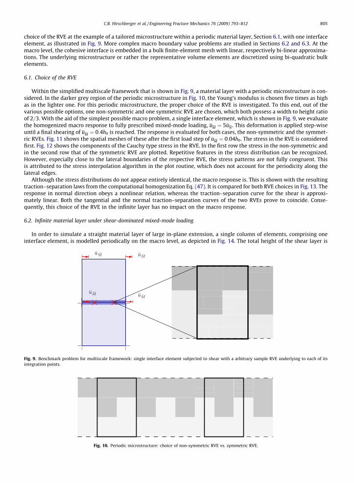
choice of the RVE at the example of a tailored microstructure within a periodic material layer, Section 6.1, with one interfaceelement, as illustrated in Fig. 9. More complex macro boundary value problems are studied in Sections 6.2 and 6.3. At themacro level, the cohesive interface is embedded in a bulk finite-element mesh with linear, respectively bi-linear approxima-tions. The underlying microstructure or rather the representative volume elements are discretized using bi-quadratic bulkelements.

6.1. Choice of the RVE

Within the simplified multiscale framework that is shown in Fig. 9, a material layer with a periodic microstructure is con-sidered. In the darker grey region of the periodic microstructure in Fig. 10, the Young’s modulus is chosen five times as highas in the lighter one. For this periodic microstructure, the proper choice of the RVE is investigated. To this end, out of thevarious possible options, one non-symmetric and one symmetric RVE are chosen, which both possess a width to height ratioof 2=3. With the aid of the simplest possible macro problem, a single interface element, which is shown in Fig. 9, we evaluatethe homogenized macro response to fully prescribed mixed-mode loading, �uM ¼ 5�uN . This deformation is applied step-wiseuntil a final shearing of �uM ¼ 0:4h0 is reached. The response is evaluated for both cases, the non-symmetric and the symmet-ric RVEs. Fig. 11 shows the spatial meshes of these after the first load step of �uM ¼ 0:04h0. The stress in the RVE is consideredfirst. Fig. 12 shows the components of the Cauchy type stress in the RVE. In the first row the stress in the non-symmetric andin the second row that of the symmetric RVE are plotted. Repetitive features in the stress distribution can be recognized.However, especially close to the lateral boundaries of the respective RVE, the stress patterns are not fully congruent. Thisis attributed to the stress interpolation algorithm in the plot routine, which does not account for the periodicity along thelateral edges.

Although the stress distributions do not appear entirely identical, the macro response is. This is shown with the resultingtraction–separation laws from the computational homogenization Eq. (47). It is compared for both RVE choices in Fig. 13. Theresponse in normal direction obeys a nonlinear relation, whereas the traction–separation curve for the shear is approxi-mately linear. Both the tangential and the normal traction–separation curves of the two RVEs prove to coincide. Conse-quently, this choice of the RVE in the infinite layer has no impact on the macro response.

6.2. Infinite material layer under shear-dominated mixed-mode loading

In order to simulate a straight material layer of large in-plane extension, a single column of elements, comprising oneinterface element, is modelled periodically on the macro level, as depicted in Fig. 14. The total height of the shear layer is

Fig. 9. Benchmark problem for multiscale framework: single interface element subjected to shear with a arbitrary sample RVE underlying to each of itsintegration points.

Fig. 10. Periodic microstructure: choice of non-symmetric RVE vs. symmetric RVE.

Fig. 11. Spatial meshes of (a) non-symmetric RVE vs. (b) symmetric RVE at �uM ¼ 5�uN ¼ 0:04h0.

Fig. 12. Cauchy stress components for (a) non-symmetric and (b) symmetric RVE.

Fig. 13. Traction–separation curve with (a) non-symmetric and (b) symmetric RVE.


Fig. 14. Infinite periodic shear layer including material layer: multiscale boundary value problem.


given as H0 ¼ 20h0. For opposite nodes at the left and right side, periodic deformations are enforced. In this way, the columnrepresents a small portion of a layer with ideally infinite in-plane extension. The deformation of the problem is prescribed atthe top and the bottom (�upre;T ¼ ��upre;B), in a shear-dominated mixedmode, with the horizontal or rather tangential displace-ment being ten times the tensile or rather normal displacement. This deformation is applied step-wise, until a final tangen-tial deformation of �u pre;T

M¼ 0:2 �w0 is reached.

Different micro meshes are examined: First, microstructures with a void of different shape and size are simulated andcompared to the response of a homogeneous microstructure. Thereafter, the shear layer is investigated with RVEs containinginclusions of higher stiffness and different distributions. At the macro level, bi-linear shape functions are used.

6.2.1. Microstructures with voidsThe problem is first studied for microstructures with voids. A homogeneous RVE of width w0 ¼ 0:1h0 is compared with

two square RVEs with each containing a centred circular hole of 5% and 25% void ratio, respectively, and another square spec-imen with a centred lentil-shaped void. These microstructures are discretized with bi-linear finite elements. The macromaterial parameters are chosen to be E ¼ 100E, �m ¼ m ¼ 0:3.

For a macro displacement load of �upre;T ¼ ��upre;B ¼ 0:2 �w0M þ 0:02 �w0N, in Fig. 15b–d the respective spatial macro meshesare plotted, whereas the corresponding spatial micro meshes are shown in Fig. 16. Based on the different size and shape ofthe voids, the stiffness of the specimen differs. This is qualitatively reflected in the deformed meshes. The weaker the RVEreacts, the stronger is the deformation localized in the material layer. The differently stiff response is quantitatively analyzedin Fig. 17. The force–displacement curves in tangential and normal direction are evaluated for the top nodes of the macrospecimen. The specimen with the lens-shaped void yields the least stiff response, whereas for decreasing size of the void,the stiffness increases.

6.2.2. Microstructures with inclusionsNext, underlying to the material layer situated within the periodic macro shear layer, microstructures equipped with

inclusions are examined. These possess a greater stiffness than the surrounding matrix material in the material layer. Thedifferent material meshes are schematized in Fig. 18. In the darker elements, Young’s modulus is chosen five times thatof the light-grey elements, E2 ¼ 5E1 ¼ E=200, while Poisson’s ratio is chosen equally as �m ¼ m1 ¼ m2 ¼ 0:3.

As for the microstructures with voids in Section 6.2.1, the force–displacement curves at the top of the macro specimen arecompared here in Fig. 19. Depending on the size and distribution of the inclusions, the resulting macroscopic force–displace-ment curves differ from each other. As expected, the specimen with the largest inclusion ratio, Fig. 18b, exhibits the stiffestbehaviour.

Fig. 15. Shear layer with interface: (a) material macro mesh; spatial macro mesh at �uM ¼ 0:2 �w0 for different microstructures: (b) benchmark homogeneousmicrostructure, (c) 5% void, (d) 25% void and (e) lens-shaped void.

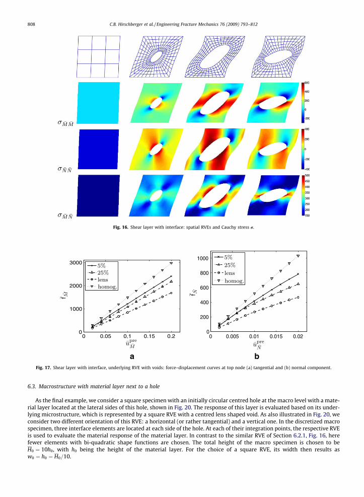
Fig. 16. Shear layer with interface: spatial RVEs and Cauchy stress r.

Fig. 17. Shear layer with interface, underlying RVE with voids: force–displacement curves at top node (a) tangential and (b) normal component.


6.3. Macrostructure with material layer next to a hole

As the final example, we consider a square specimen with an initially circular centred hole at the macro level with a mate-rial layer located at the lateral sides of this hole, shown in Fig. 20. The response of this layer is evaluated based on its under-lying microstructure, which is represented by a square RVE with a centred lens shaped void. As also illustrated in Fig. 20, weconsider two different orientation of this RVE: a horizontal (or rather tangential) and a vertical one. In the discretized macrospecimen, three interface elements are located at each side of the hole. At each of their integration points, the respective RVEis used to evaluate the material response of the material layer. In contrast to the similar RVE of Section 6.2.1, Fig. 16, herefewer elements with bi-quadratic shape functions are chosen. The total height of the macro specimen is chosen to beH0 ¼ 10h0, with h0 being the height of the material layer. For the choice of a square RVE, its width then results asw0 ¼ h0 ¼ H0=10.

Fig. 18. RVEs for microstructure with inclusions: (a)–(c) material meshes with heterogeneous material properties and (d)–(e) corresponding spatialmeshes.

Fig. 19. Macro force–displacement curves, (a) tangential and (b) normal components.

Fig. 20. Multiscale boundary value problem with the two RVEs under investigation, material finite-element mesh: Macro specimen with circular void andhorizontal interface layer, RVE (a) with horizontally and RVE (b) with vertically oriented lens-shaped void.



In order to identify the respective spatial RVEs assigned to the interface element integration points along the interfaceelement, we introduce the coordinate N ¼ 2XM= �w0 that denotes the relative initial location compared to half the width ofthe macro specimen as illustrated in Fig. 20. Fig. 21 displays the corresponding spatial RVE meshes at the integration point

Fig. 21. Spatial RVE meshes along the interface at interface integration point coordinates Ni ¼ 0:522; 0:581; 0:638; 0:737; 0:821; 0:952: (a) horizontally and(b) vertically oriented lens-shaped void.

Fig. 22. (a) Spatial macro mesh, (b) traction–separation curve at point N ¼ 0:522, (c) separation and (d) traction over the integration point position N alongthe interface.


coordinates. Knowing that the model prevents a lateral deformation of the RVE, we observe that the RVE with the horizon-tally oriented void undergoes larger deformations in loading direction. This qualitative result is supported by the quantita-tive curves in Fig. 22. Here, besides the spatial macro mesh, the corresponding homogenized tractions �tN and the separationss �uNt at these macro Gauss points are plotted vs. their position N. As expected, closer to the macroscopic hole, both the trac-tion and the deformation increase more steeply. Furthermore, the orientation of the lens-shaped void plays a significant role.The horizontally oriented void attracts more separation and less traction, while the slope of the traction–separation curve isless steep. Consequently, this specimen involves a weaker response than that with the vertically oriented void. This is alsoreflected in the two resulting traction–separation curves at the macro integration point closest to the hole, �tN vs. s�uNt. It canbe observed that by their orientation, heterogeneities in the microstructure can yield anisotropic effects in the global re-sponse of the material layer.

7. Conclusion

In this contribution, we have proposed a computational homogenization approach for a microscopically heterogeneousmaterial layer. On the basis of the underlying microstructural constitution, the macroscopic response of a body containingthis material layer is efficiently determined. The proposed approach is based on a continuum mechanics framework at finitedeformations with a cohesive interface to represent the material layer. Based on existing continuum homogenization prin-ciples, the vectorial quantities traction and separation at the macro level have been related to the averaged tensorial stressand deformation gradient at the micro level. The height of the representative volume element has been considered as theheight of the material layer itself. Thus this quantity enters the equivalence of the virtual work of both scales. The possibletensile and shear deformation modes in the interface have been accounted for through customized boundary conditions onthe representative volume element, which are hybrid between prescribed deformation out of the plane and periodic defor-mation in the plane of the interface. The developed theoretical framework has been successfully embedded in a computa-tional homogenization procedure that couples the macroscopic and the microscopic response in an iterative nestedsolution procedure. Numerical examples have revealed that the macroscopic response depends on the particular geometryand material properties of the respective microstructure. With the continuous representative volume element and the cus-tomized hybrid boundary conditions, mixed-mode loading is captured in a natural manner. Additionally to existing ap-proaches to mixed-mode response, e.g., of Refs. [29,36], the behaviour here is dictated by its microstructure rather thanby an a priori constitutive assumption.

Some challenges for future research evolve from this contribution, either concerning the constitutive/continuum formula-tion or the numerical framework. First of all, in addition to the hyperelastic constitutive format chosen here, the incorporationof irreversible behaviour within the microstructure, as done in Ref. [17] for small strain, for finite strains remain as a challengefor future research. Only such choices can render the typical traction–separation laws expected based on Refs. [27,38]. Thepresent multiscale framework with the classical continuum within the RVE does not account for size effects, which can occurwhen a significant intrinsic microstructure in the interfacial material coincides with a particularly thin material layer. In suchcases, we suggest to employ a generalized continuum as for instance a micromorphic or higher-gradient continuum on theRVE level, as pursued in Ref. [7]. One limitation of the multiscale model, which we have particularly identified in the lastnumerical example, is the fact that although at the macro level there is no obstacle to a lateral contraction of the material layer,the present homogenization framework provides no option to pass this lateral contraction to the underlying representativevolume element or vice versa to incorporate the resistance of the RVE against lateral contraction into the homogenization.Recognizing this limitation, it remains as a non-trivial task for future research to enhance the micro–macro transition in thisrespect such that also a lateral contraction can be taken into account appropriately whenever it is needed.

The interface elements used to model the cohesive layer at the macro level could be used in a wider range of boundaryvalue problems, once contact algorithms to capture compression in the interface are implemented. It is noteworthy that theproposed computational homogenization for material layers is not only restricted to finite interface elements, but can beemployed whenever a constitutive relation for a cohesive layer is to be evaluated at an integration point. When the proposedcomputational homogenization framework is combined with more elaborate approaches to treat discontinuous deforma-tions, such as the partition-of-unity based X-FEM [26] or approaches based on Nitsche’s method [19], it has potential to serveas a powerful multiscale tool in the simulation of cohesive discontinuities which are governed by their underlying hetero-geneous microstructure.

Acknowledgement

The authors gratefully acknowledge financial support by the German Science Foundation (DFG) within the InternationalResearch Training Group 1131 ‘Visualization of large and unstructured data sets. Applications in geospatial planning, modeling,and engineering’ and the Research Training Group 814 ‘Engineering materials on different scales: Experiment, modelling, andsimulation’.


References

[1] Beer G. An isoparametric joint/interface element for finite element analysis. Int J Numer Meth Engng 1985;21:585–600.[2] Costanzo F, Gray GL, Andia PC. On the definitions of effective stress and deformation gradient for use in MD: Hill’s macro-homogeneity and the virial

theorem. Int J Numer Meth Engng 2005;43:533–55.[3] Feyel F, Chaboche J-L. FE2 multiscale approach for modelling the elastoviscoplastic behaviour of long fibre SiC/Ti composites materials. Comput Meth

Appl Mech Engng 2000;183:309–30.[4] Hill R. Elastic properties of reinforced solids: some theoretical principles. J Mech Phys Solid 1963;11:357–72.[5] Hill R. On constitutive macro-variables for heterogeneous solids at finite strain. Proc Roy Soc Lond A 1972;326:131–47.[6] Hirschberger CB. A treatise on micromorphic continua. Theory, homogenization, computation. PhD thesis, University of Kaiserslautern; 2008. ISSN

1610–4641, ISBN 978–3–939432–80–7.[7] Hirschberger CB, Sukumar N, Steinmann P. Computational homogenization of material layers with micromorphic mesostructure. Phil Mag 2008,

accepted for publication.[8] Kouznetsova VG. Computational homogenization for the multiscale analysis of multi-phase materials. PhD thesis, Eindhoven University of Technology;

2002.[9] Kouznetsova VG, Brekelmans WAM, Baaijens FPT. An approach to micro–macro modeling of heterogeneous materials. Comput Mech 2001;27:37–48.

[10] Kouznetsova VG, Geers MGD, Brekelmans WAM. Multi-scale constitutive modelling of heterogeneous materials with a gradient-enhancedcomputational homogenization scheme. Int J Numer Meth Engng 2002;54:1235–60.

[11] Kouznetsova VG, Geers MGD, Brekelmans WAM. Multi-scale second-order computational homogenization of multi-phase materials: a nested finiteelement solution strategy. Comput Meth Appl Mech Engng 2004;193:5525–50.

[12] Larsson R, Runesson K, Ottosen NS. Discontinuous displacement approximation for capturing plastic localization. Int J Numer Meth Engng1993;36:2087–105.

[13] Larsson R, Runesson K, Sture S. Finite element simulation of localized plastic deformation. Arch Appl Mech 1991;61:305–17.[14] Larsson R, Zhang Y. Homogenization of microsystem interconnects based on micropolar theory and discontinuous kinematics. J Mech Phys Solid

2007;55:819–41.[15] Lebon F, Ould Khaoua A, Licht C. Numerical study of soft adhesively bonded joints in finite elasticity. Comput Mech 1998;21:134–40.[16] Lebon F, Rizzoni R, Ronel-Idrissi S. Asymptotic analysis of some non-linear soft layers. Comput Struct 2004;82:1929–38.[17] Matous K, Kulkarni MG, Geubelle PH. Multiscale cohesive failure modeling of heterogeneous adhesives. J Mech Phys Solid 2008;56:1511–33.[18] Mergheim J, Kuhl E, Steinmann P. A hybrid discontinuous Galerkin/interface method for the computational modelling of failure. Commun Numer Meth

Engng 2004;20:511–9.[19] Mergheim J, Kuhl E, Steinmann P. A finite element method for the computational modelling of cohesive cracks. Int J Numer Meth Engng

2005;63:276–89.[20] Michel JC, Moulinec H, Suquet P. Effective properties of composite materials with periodic microstructure: a computational approach. Comput Meth

Appl Mech Engng 1999;172:109–43.[21] Miehe C. Computational micro-to-macro transitions discretized micro-structures of heterogeneous materials at finite strains based on the

minimization of averaged incremental energy. Comput Meth Appl Mech Engng 2003;192:559–91.[22] Miehe C, Koch A. Computational micro-to-macro transitions of discretized microstructures undergoing small strains. Arch Appl Mech 2002;72:300–17.[23] Miehe C, Schröder J. Post-critical discontinuous localization analysis of small-strain softening elastoplastic solids. Arch Appl Mech 1994;64:267–85.[24] Miehe C, Schröder J, Bayreuther C. On the homogenization analysis of composite materials based on discretized fluctuations on the micro-structure.

Comput Mater Sci 2002;155:1–16.[25] Miehe C, Schröder J, Schotte J. Computational homogenization analysis in finite plasticity. Simulation of texture development in polycrystalline

materials. Comput Meth Appl Mech Engng 1999;171:387–418.[26] Moës N, Dolbow J, Belytschko T. A finite element method for crack growth without remeshing. Int J Numer Meth Engng 1999;46:131–50.[27] Needleman A. A continuum model for void nucleation by inclusion debonding. J Appl Mech 1987;54:525–31.[28] Nemat-Nasser A, Hori M. Micromechanics: overall properties of heterogeneous materials. 2nd ed. North-Holland: Elsevier; 1999.[29] Ortiz M, Pandolfi A. Finite-deformation irreversible cohesive elements for three-dimensional crack-propagation analysis. Int J Numer Meth Engng

1999;44:1267–82.[30] Schellekens JCJ, de Borst R. On the numerical integration of interface elements. Int J Numer Meth Engng 1993;36:43–66.[31] Steinmann P. A model adaptive strategy to capture strong discontinuities at large inelastic strain. In: Idelsohn S, Oñate E, Dvorking E, editors.

Computational mechanics. New trends and applications, CIMNE, Barcelona; 1998. p. 1–12.[32] Steinmann P, Betsch P. A localization capturing FE-interface based on regularized strong discontinuities at large inelastic strains. Int J Solid Struct

2000;37:4061–82.[33] Sukumar N, Pask JE. Classical and enriched finite element formulations for Bloch-periodic boundary conditions. Int J Numer Meth Engng. doi:10.1002/

nme.2457.[34] Utzinger J, Bos M, Floeck M, Menzel A, Kuhl E, Renz R, et al. Computational modelling of thermal impact welded PEEK/steel single lap tensile

specimens. Comput Mater Sci 2008;41(3):287–96.[35] Utzinger J, Menzel A, Steinmann P, Benallal A. Aspects of bifurcation in an isotropic elastic continuum with orthotropic inelastic interface. Eur J Mech A

Solid 2008;27:532–47.[36] van den Bosch MJ, Schreurs PJG, Geers MGD. An improved description of the exponential Xu and Needleman cohesive zone law for mixed-mode

decohesion. Engng Fract Mech 2006;73:1220–34.[37] van den Bosch MJ, Schreurs PJG, Geers MGD. On the development of a 3d cohesive zone element in the presence of large deformations. Comput Mech

2008;42:171–80.[38] Xu X-P, Needleman A. Void nucleation by inclusion debonding in a crystal matrix. Model Simul Mater Sci Engng 1993;1:111–32.

http://dx.doi.org/10.1002/nme.2457

http://dx.doi.org/10.1002/nme.2457

engineering fracture mechanics - materials technology multiscale modelling of heterogeneous material...

Documents