1

ENGINEERING MATHEMATICS-II

FUNCTION,LIMIT,CONTINUITY,DIFFERENTIATION AND ITS

APPLICATIONS

Dr A K Das, Sr. Lecturer in Mathematics

U C P Engineering School Berhampur

2

1.LIMIT OF A FUNCTION

Lets discuss what a function is

A function is basically a rule which associates an element with another

element.

There are different rules that govern different phenomena or happenings in

our day to day life.

For example,

i. Water flows from a higher altitude to a lower altitude

ii. Heat flows from higher temperature to a lower temperature.

iii. External force results in change state of a body(Newton’s 1st Rule of

motion) etc.

All these rules associates an event or element to another event or element,

say , x with y.

Mathematically we write,

y = f(x)

i.e. given the value of x we can determine the value of y by applying the rule

‘f’

for example,

i.e we calculate the value of y by adding 1 to value of x. This is the rule or

function we are discussing.

Since we say a function associates two elements, x and y we can think of

two sets A and B such that x is taken from set A and y is taken from set B.

Symbolically we write

x A ( x belongs to A)

3

y B ( x belongs to B)

y = f(x) can also be written as

(x,y) f

Since (x,y) represents a pair of elements we can think of these in relations

f A X B or

f can thought of as a sub set of the product of sets A and B we have earlier

referred to.

And, therefore, the elements of f are pair of elements like (x,y).

In the discussion of a function we must consider all the elements of set A

and see that no x is associated with two different values of y in the set B

What is domain of function

Since function associates elements x of A to elements y of B and function

must take care of all the elements of set A we call the set A as domain of

the function. We must take note of the fact that if the function can not be

defined for some elements of set A , the domain of the function will be a

subset of A.

Example 1

Let A = { }

B = { }

The function is given by

y = f(x) = x + 1

for x=1, y= 2

x=2, y=3

x=3,y=4

x=4,y=5

4

x=-1,y=0

x=0,y=1

x=-4,y=-3

clearly y=5 and y= -3 do not belong to set B. therefore we say the domain of

this function is

the set { } which is a sub set of set A.

What is range of a function

Range of the function is the set of all y’s whose values are calculated by

taking all the values of x in the domain of the function. Since the domain of

the function is either is equal to A or sub set of set A, range of the function

is either equal to set b or sub set of set B.

In the earlier example,

Range of function is the set { } which is a sub set of set B

SOME FUNDAMENTAL FUNCTIONS

Constant Function

Y = f(x)=K, for all x

The rule here is: the value of y is always k, irrespective of the value of x

This is a very simple rule in the sense that evaluation of the value of y is not

required as it is already given as k

Domain of ‘f’ is set of all real numbers

Range of ‘f’ is the singleton set containing ‘k’ alone.

Or

Dom= R, set of all real numbers

Range= {k}

Graph of Constant Function

5

Let y = f(x) = k =2.5

The graph is a line parallel to axis of x

Identity Function

Y = f(x)=x, for all x

The rule here is: the value of y is always equals to x

This is also a very simple rule in the sense that the value of y is identical

with the value of x saving our time to calculate the value of y.

Dom = R

Range = R

i.e. Domain of the function is same as Range of the function

Graph of Identity Function

0

1

2

3

-3 -2 -1 0 1 2 3 4 5

y ax

is

x axis

-3, -3 -2, -2

-1, -1 0, 0

1, 1 2, 2

3, 3

-4

-2

0

2

4

-4 -3 -2 -1 0 1 2 3 4Axi

s Ti

tle

Axis Title

6

Modulus Function

( ) | | {

}

The rule here is: the value of y is always equals to the numerical value of x,

not taking in to consideration the sign of x.

Example

Y =f(2)=2

Y=f(0)=0

Y=f(-3)=3

This function is usually useful in dealing with values which are always

positive for example, length, area etc.

Dom = R

Range = R+ U { }

Graph of Modulus Function

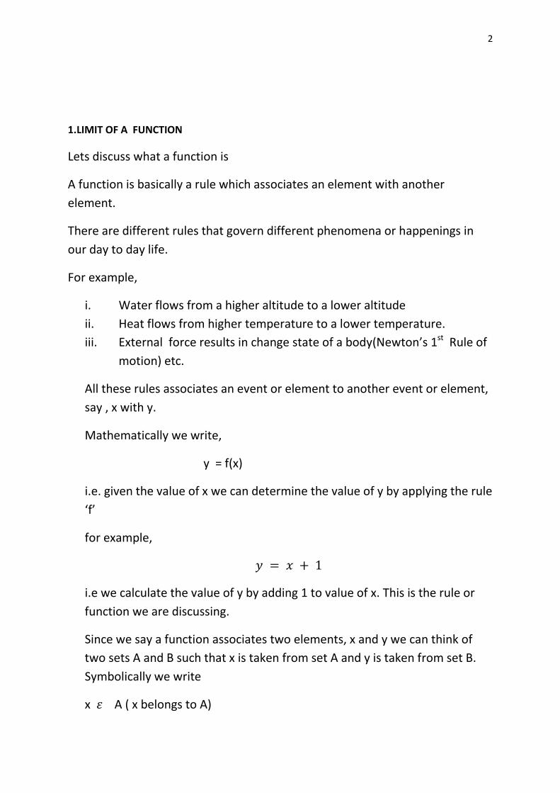
Signum Function

( ) {| |

} {

}

This is also a very simple rule in the sense that the value of y is 1 if x is

positive , 0 when x=0, and -1 when x is negative.

0

1

2

3

4

5

-6 -4 -2 0 2 4 6

y A

xis

x Axis

7

Dom = R

Range = { }

Graph of Signum Function

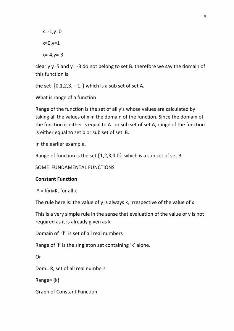
Greatest Integer Function

( ) [ ]

For Example [ ] [ ] [ ] [ ]

Dom = R

Range=Z(set of all Integers)

Graph of The function

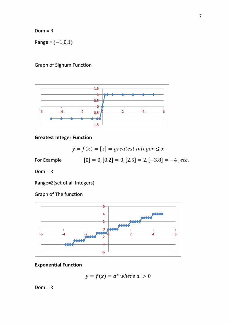
Exponential Function

( )

Dom = R

-1.5

-1

-0.5

0

0.5

1

1.5

-6 -4 -2 0 2 4 6

-6

-4

-2

0

2

4

6

-6 -4 -2 0 2 4 6

8

Range= R+

The specialty of the function is that whatever the value of x, y can never be

0 or negative

Graph of Exponential Function

Logarithmic Function

( )

Dom = R+

Range =

Graph of Logarthmic Function

0

5

10

15

20

-2 -1 0 1 2 3 4 5

y a

xis

x Axis

y=2x

0

5

10

15

20

-5 -4 -3 -2 -1 0 1 2

y A

xis

x Axis

y=(0.5)x

-4

-2

0

2

4

0 1 2 3 4 5 6y A

xis

x Axis

y = log x

9

-3

-2

-1

0

1

2

3

4

0 1 2 3 4 5 6

y = log x

10

LIMIT OF A FUNCTION

Consider the function

y =2 x + 1

lets see what happens to value of y as the value of x changes.

Lets take the values of x close to the value of, say, 2. Now when we say

value of x close 2. It can be a value like 2.1 or 1.9. in one case it is close to 2

but greater than 2 and in other it is close to 2 but less than 2.Now consider

a sequence of such numbers slightly greater than 2 and slightly less than 2

and accordingly calculate the value of y in each case.

Look at the table

x y=2x+1

1.9 4.8 1.91 4.82

1.92 4.84 1.93 4.86

1.94 4.88

1.95 4.9 1.96 4.92

1.97 4.94 1.98 4.96

1.99 4.98 2.01 5.02

2.02 5.04

2.03 5.06 2.04 5.08

2.05 5.1 2.06 5.12

2.07 5.14

2.08 5.16 2.09 5.18

2.1 5.2

11

We see in the tabulated value that

as x is approaching the value of 2 from either side, the value of y is

approaching the value of 5

in other words we say,

y → 5 (y tends to 5) as x → 2(x tends to 2) or

INFINITE LIMIT

As x→ a for some finite value of a, if the value of y is greater than any positive

number however large then we say

Y → ∞ (y tends to infinity)

In other words y is said have an infinite limit as x → a. And we write

Example

If

,

Then

Since x→0, is positive,

becomes very very large and is positive. Therefore the result.

Similarly,

As x→ a for some finite value of a, if the value of y is less than any negative

number however large then we say

Y →- ∞ (y tends to minus infinity)

12

In other words y is said have an infinite limit as x → a. And we write

Example

If

,

Then

Since x→0, is positive,

becomes very very large and is negative. Therefore the result.

LIMIT AT INFINITY

As x becomes very very large or in other words the value of x is greater than a

very large positive number , i.e. x → ∞, if value of y is close to a finite value’ a’,

then we say has a finite limit ‘a’ at infinity and write

Example

Let

As x→∞ ,

becomes very very small and approaches the value 0.Therefore

we write

13

similarly

As x becomes very very large with a negative sign or in other words the value

of x is less than a very large negative number , i.e. x →- ∞, if value of y is close

to a finite value’ a’, then we say has a finite limit ‘a’ at infinity and write

Example

Let

As x→∞ ,

becomes very very small and approaches the value 0.Therefore

we write

ALGEBRA OF LIMITS

1. Limit of sum of two functions is sum of their individual limits

Let ( ) ( ) , then

( ( ) ( ))

2.Limit of product of two functions is product of the their individual limits

Let ( ) ( ) , then

( ( ) ( ))

3. Limit of quotient of two functions is quotient of the their individual

limits

Let ( ) ( ) , then

( )

( )

14

SOME STANDARD LIMITS

1. ( ) ( ) where P(x) is polynomial in x

Example

( )

2.

where n is a rational number

Example

3. (

)

,

(

)

,

4. ( )

( )

5. (

)

Example

. (

)

6. ( )

Example

( )

15

SOME STANDARD TRIGONOMETRIC LIMITS

1

2.

3.

4.

, here

5.

Example

Since

Example

( )

( )

( )

16

Example

( )

(

) (

)

Existence of Limits

When we say x tends to ‘a’ or write x→a it can happen in two different ways

X can approach ‘a’ through values greater than ‘a’ i.e from right side of ‘a’ on

the Number Line

Or

X can approach ‘a’ through values smaller than ‘a’ i.e from left side of ‘a’ on the

Number Line

The first case is called the Right Hand Limit and the later case is called the Left

Hand Limit.

We, therefore conclude that Limit will exist iff the right Hand Limit and the Left

Hand Limit both exist and are EQUAL

Consider the Greatest Integer Function

( ) [ ]

Consider the limit of this function as

The right hand limit of this function

[ ]

Since if the value of x is greater than 1 for example 1+h,h then the greatest

integer less than equal to 1+h is 1

The left hand limit of this function

[ ]

17

Since if the value of x is less than 1 for example 1-h,h , then the greatest

integer less than equal to 1-h is 0

In this case the right hand limit and the left hand limit are not equal

And therefore the limit of this function as does not exist

For that matter this function does not allow limit as

Since the right hand limit will be always n and the left hand limit will be n-1.

Consider the Signum Function

( ) {| |

} {

}

Consider the limit of this function as

The right hand limit of this function is 1 and the left hand limit of this function

is -1 as evident from the definition of the function and concept of right and left

hand limits

Therefore this function does not have a limit as

0

0.5

1

1.5

0 0.5 1 1.5 2

-1.5

-1

-0.5

0

0.5

1

1.5

-1.5 -1 -0.5 0 0.5 1 1.5

18

Continuity of function

A function is continuous at a point ‘c’ iff its functional value i.e the value of

the function at the point ‘c’ is same as limiting value of the function i.e value

of the limit evaluated at the point ‘c’

OR

( ) ( )

This means that a function is continuous at a point ‘c’ iff

All the three conditions mentioned below holds good

1.limit of the function as exists

2.the function has a value at x=c. i.e f(c) does exist

3.the limit of the function is equal to value of the function at the point x=c

Most of the functions we encounter are continuous functions

For example

The physical growth of a child is a continuous function

The distance travelled is a continuous function of time

Continuous functions are easy to handle in the sense that we can predict the

value at an latter stage. For example if the education of a child is continuous

we can predict what he or she might be reading after say 5 years.

Examples

The constant function is continuous at any point ‘c’ and hence is continuous

everywhere.

( )

( )

Consider the Function

( )

19

This function is not continuous at x=4.Since the function is not defined at x=4

Consider another Function

( ) [ ]

Consider the point x=2

This function does not have limit x → 2 as the Right Hand limit will be 2 and the

Left Hand Limit will be 1.Hence this function is also not continuous at x = 2

Example

( ) {

( )

( ) ( )

i.e

( ) ( )

This function is therefore continuous at x=4

Limiting value is same as functional value

Consider another Function

( ) {(

)

( )

(

)

[(

)

]

( ) ( )

i.e

limit of the function is same as value of the function at the point

20

therefore, the function is continuous at x=0

example

consider the function

( ) {

Consider the point x=0

( )

( )

Therefore the function is continuous at x=0

As,

|

| | |

Taking limit as x we can conclude that

21

Differentiation

A function f(x) is said to be differentiable at a point x=c iff

( ) ( )

In general, a function is differentiable iff

( ) ( )

Once this limit exists, it is called the differential coefficient of f(x) or the

derivative of the function f(x) at x=c

Or

( ) ( )

( )

( ) ( )

( )

Where ( ) and ( ) are the differential coefficient or the derivative of the

function, the first being defined at x=c

Examples

Consider the function

( )

In this case the differential coefficient ( )is given by

( )

( ) ( )

Therefore the constant function is differentiable everywhere and the

derivative is zero

22

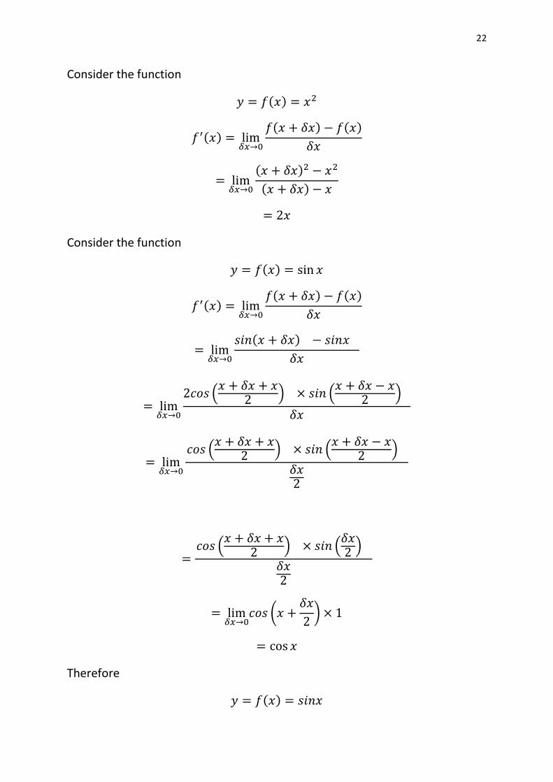
Consider the function

( )

( )

( ) ( )

( )

( )

Consider the function

( )

( )

( ) ( )

( )

(

) (

)

(

) (

)

(

) (

)

(

)

Therefore

( )

23

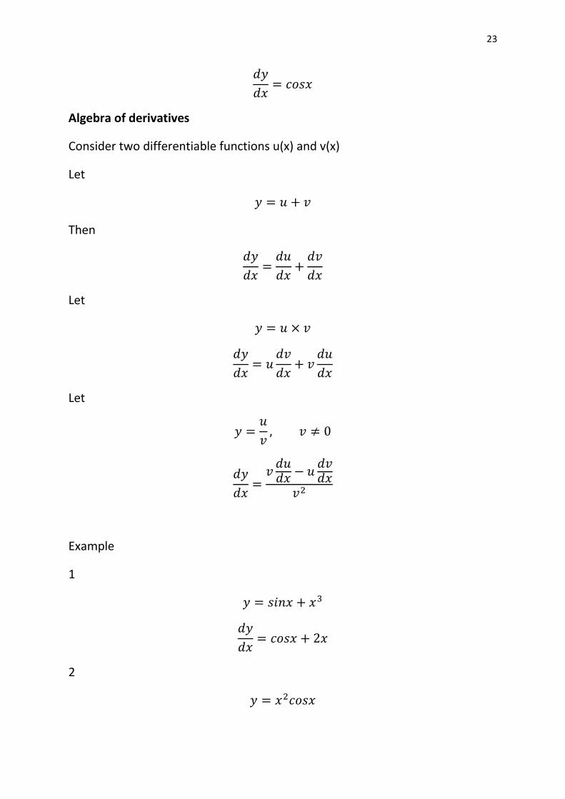
Algebra of derivatives

Consider two differentiable functions u(x) and v(x)

Let

Then

Let

Let

Example

1

2

24

( ) ( )

3

( )

( )

( ) ( )

( )

( ) ( )

( )

( ) ( )

Geometrical meaning of ( )

Consider the graph of a function

( )

25

( ) ( )

Represents the ratio of height to base of the angle the line joining the point

P(c,f(c )) and Q (c+h,f(c+h))

i.e

( ) ( )

Where is the angle the line joining the point P and Q makes with the positive

direction of x axis.

In the limiting case as h i.e as Q the line PQ becomes the tangent line

and the the angle which the tangent line makes with

the positive direction of x axis

i.e

( ) ( )

( ) ( )

Application to Geometry

To find the equation of the tangent line to the curve y=f(x) at x=

The equation of line passing through the point ( ( )) is give by

( ) ( )

Where ‘ m’ is the slope of the tangent line.

As, we have seen

( )

The equation is therefore

( ) ( )( )

In the above example if we take

( )

26

The equation to the tangent at the point is given by

( ) ( )( )

Or

( )

where

( ) ( )

i.e

the equation is

( )

Derivative as rate measurer

Remember the definition

( ) ( )

( )

The quantity

( ) ( )

( )

Consider the linear motion of a particle given as

( )

Where ‘s’ denotes the distance traversed and ‘t’ denotes the time taken

The ratio

Denotes the average velocity of the particle

To calculate the local velocity or instantaneous velocity at a point of time

t= we proceed in the following way

27

Consider an infinitesimal distance ’ traversed from time t= in time ’

The ratio

Still represents a average value of the velocity

The instantaneous velocity at t= can be calculated by considering the

following limit

or

Where ‘v’ represents the instantaneous velocity which is defined as rate of

change of displacement

Similarly, we can write the mathematical expression for acceleration

As

Or the rate of change of velocity

Example

If the motion of a particle is given by

( )

Which is linear in nature, we can calculate velocity at t=3

( )

It is clear that the velocity is independent of time ‘t’.

28

i.e

the above motion has constant or uniform velocity.

And, therefore, the acceleration

Or the motion does not produce any acceleration.

Consider another motion of a particle given as

( )

Here the velocity at t=3 can be calculated as

( )

And the acceleration

Therefore we can say that the motion is said to have constant or uniform

acceleration

Derivatives of implicit function

Consider the equation of a circle

This is an implicit function

Lets differentiate this equation with respect x throughout, we get

29

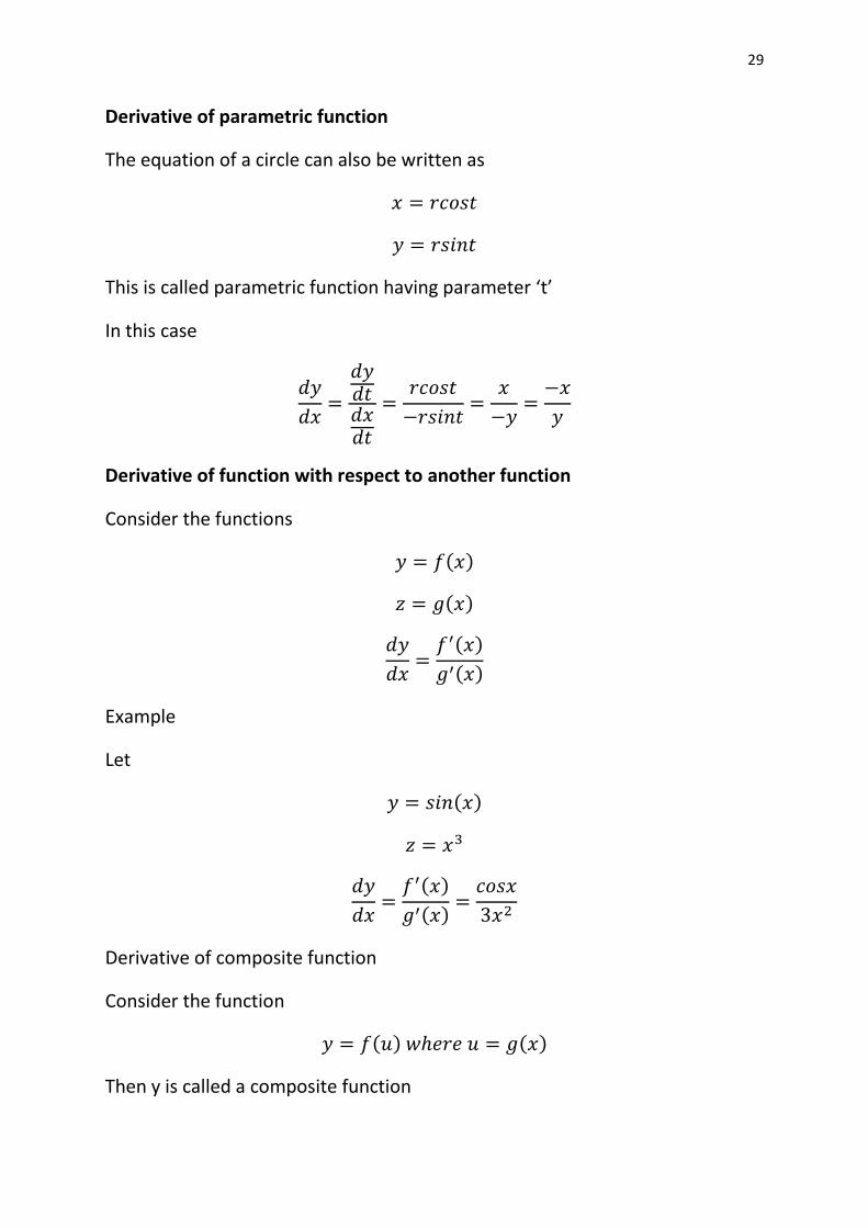
Derivative of parametric function

The equation of a circle can also be written as

This is called parametric function having parameter ‘t’

In this case

Derivative of function with respect to another function

Consider the functions

( )

( )

( )

( )

Example

Let

( )

( )

( )

Derivative of composite function

Consider the function

( ) ( )

Then y is called a composite function

30

In this case

This is called Chain Rule. This can be extended to any number of functions.

Example

1.Let

This can be written as

And

Applying chain rule, we have

2.Let

This can be written as

And

Applying chain rule, we have

31

Derivatives of inverse function

As

Which follows from the fact that

( )

And the condition of continuity guarantees the above fact.

Derivative of inverse trigonometric function

Let

Where (

)

This can be written as

Or

( )

( )

( )

Since cosy is positive in the domain

32

Let

Where ( )

This can be written as

Or

( )

( )

( )

Since sin y is positive in the domain

Let

Where (

) (

)

This can be written as

Or

( )

( √( ))

| | ( )

Since is positive in the domain

Let

33

Where (

) (

)

This can be written as

Or

( )

( √( ))

| | ( )

Since is positive in the domain

Let

This can be written as

Or

Let

This can be written as

34

Or

Higher order derivatives

Let

( )

Is differentiable and also

( )

Is differentiable. Then we define

(

)

( )

( ) ( )

This is the 2nd. Order derivative of the function

Similarly we can define higher order derivatives of the function

Example

Let

( )

( )

( )

35

Consider the Function

( )

Here

( )

( )

i.e in this case

Monotonic Function

Increasing function

Consider a function

( )

If ( ) ( )

Then the function is increasing

Example

( )

( )

( )

Or

( ) ( )

Therefore the function is increasing

Graph of the function

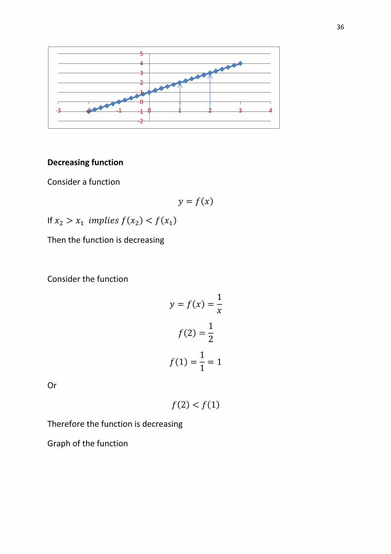
36

Decreasing function

Consider a function

( )

If ( ) ( )

Then the function is decreasing

Consider the function

( )

( )

( )

Or

( ) ( )

Therefore the function is decreasing

Graph of the function

-2

-1

0

1

2

3

4

5

-3 -2 -1 0 1 2 3 4

37

A function either increasing or decreasing is called monotonic.

Derivative of Increasing Function

If f(x) is increasing, then

( )

( ) ( )

i.e

for increasing function the derivative is always positive

Derivative of Decreasing Function

If f(x) is decreasing, then

( )

( ) ( )

i.e

for decreasing function the derivative is always negative

example

let

( )

0

1

2

3

4

5

6

0 0.5 1 1.5 2 2.5 3 3.5 4 4.5

38

( )

Therefore the function is increasing

Let

( )

( )

Therefore the function is decreasing

Let

( )

( )

Therefore the function is increasing for and decreasing for

Graph of the function

( )

0

1

2

3

4

5

-3 -2 -1 0 1 2 3

39

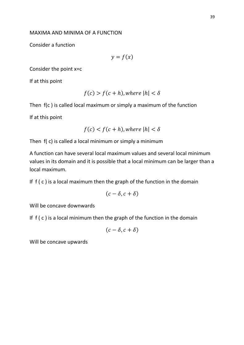
MAXIMA AND MINIMA OF A FUNCTION

Consider a function

( )

Consider the point x=c

If at this point

( ) ( ) | |

Then f(c ) is called local maximum or simply a maximum of the function

If at this point

( ) ( ) | |

Then f( c) is called a local minimum or simply a minimum

A function can have several local maximum values and several local minimum

values in its domain and it is possible that a local minimum can be larger than a

local maximum.

If f ( c ) is a local maximum then the graph of the function in the domain

( )

Will be concave downwards

If f ( c ) is a local minimum then the graph of the function in the domain

( )

Will be concave upwards

40

Maximum Case

41

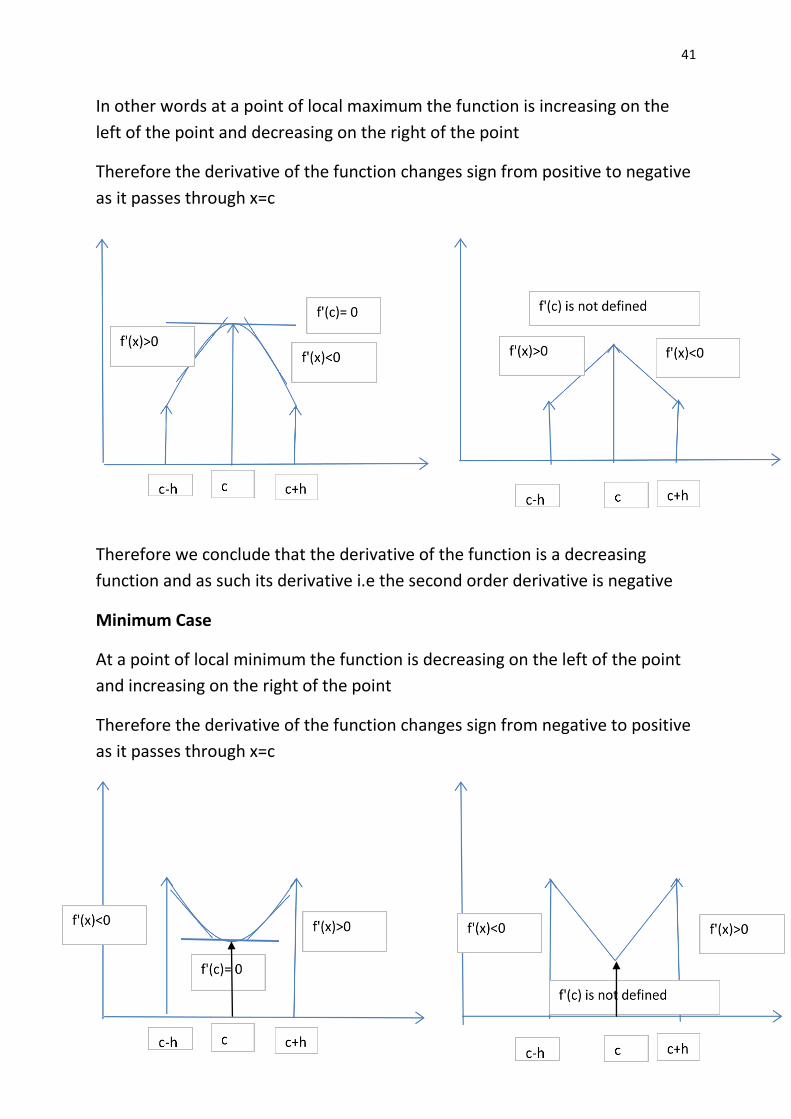
In other words at a point of local maximum the function is increasing on the

left of the point and decreasing on the right of the point

Therefore the derivative of the function changes sign from positive to negative

as it passes through x=c

Therefore we conclude that the derivative of the function is a decreasing

function and as such its derivative i.e the second order derivative is negative

Minimum Case

At a point of local minimum the function is decreasing on the left of the point

and increasing on the right of the point

Therefore the derivative of the function changes sign from negative to positive

as it passes through x=c

42

Therefore we conclude that the derivative of the function is a increasing

function and as such its derivative i.e the second order derivative is positive

In either maximum or minimum case the 1st. derivative of the function is zero

or is not defined at the point of maximum or minimum

The point x=c where the derivative vanishes or does not exist at all is called a

critical point or turning point or stationary point.

A function can have neither a maximum nor a minimum value

Example

Consider the function

( )

Here

This vanishes at x=0

And

Which also vanishes

Therefore we may conclude that the function does not have maximum neither

minimum value

43

Point of inflexion

If a curve is changing its nature from concave downwards to concave upwards

as shown in the figure or vice versa, then at the point where this change occurs

is called the point of inflexion. In other words on one side of the point of

inflexion the curve is concave downward and on the other side the curve is

concave upward or vice versa

In the above figure,

On the left side of point of inflexion a maximum value occurs and to the right

side of point of inflexion a minimum value occurs.

In other words, remembering the condition of maximum and minimum, we can

say,

The 2nd order derivative changes its sign from negative to positive as in the

case given in the figure or vice versa.

In other words the point of inflexion is the point of either maximum or

minimum of the 1st derivative of the function

Hence at the point of inflexion the 2nd. order derivative vanishes or is not

defined and the 2nd. order derivative changes its sign as it passes through the

point of inflexion

44

i.e at the point of inflexion

1.

( ) or is not defined

2. The 2nd.order derivative changes sign as it passes through the point

Example

Consider the function we discussed earleier

( )

Here

This vanishes at x=0

And

Which also vanishes at x=0

But

Therefore we conclude that

X=0 is a point of inflexion for the curve

-10

-8

-6

-4

-2

0

2

4

6

8

10

-3 -2 -1 0 1 2 3

45

Working procedure to find the maxima and minima

1.Given any function, equate the first derivative to zero to find the turning

points or critical points

2.Test the sign of the second derivative at these points. If the sign is negative it

is appoint of maximum value. If the sign is positive it is a point of minimum

value.

3. then calculate the maximum value/minimum value of the function by taking

the value of x as the point

Example

If the sum of two numbers is 10, find the numbers when their product is

maximum

Solution

Let the numbers be x and 10-x

Let

( ) ( )

Therefore the function which is the product of the numbers maximum if the

numbers are equal i.e 5 and 5.

EXAMPLE

Investigate the extreme values of the function

( )

The critical points are roots of the equation

46

( )

Or

( ) ( )

Or

Lets check the sign of the 2nd. Derivative at these points

Now,

( ) ( )

( ) ( )

Therefore x=0 is a point of maximum value.

The maximum value of the function is given as

( ) ( )

Now

( ) ( )

Therefore x = 1 is a point of minimum value.

The minimum value of the function is given as

( ) ( )

Now

( ) ( )

Therefore x = -1 is a point of minimum value.

The minimum value of the function is given as

( ) ( )

47

Prepared by

Sri. S. S. Sarcar (Sr. Lect.)

Deptt. Of Math.& Science

OSME, Keonjhar

INTEGRATION

48

INTEGRATION AS INVERSE PROCESS OF DIFFERENTIATION

Integration is the process of inverse differentiation .The branch of calculus which

studies about Integration and its applications is called Integral Calculus.

Let and be two real valued functions of such that,

Then, is said to be an anti-derivative (or integral) of . Symbolically we write∫ .

The symbol ∫ denotes the operation of integration and called the integral sign.

denotes the fact that the Integration is to be performed with respect to .The function

is called the Integrand.

INDEFINITE INTEGRAL

Let be an anti-derivative of . Then, for any constant ‘C’,

{ }

So, is also an anti-derivative of , where C is any arbitrary constant. Then,

denotes the family of all anti-derivatives of , where C is an indefinite constant.

Therefore, is called the Indefinite Integral of .

Symbolically we write

∫ ,

Where the constant C is called the constant of integration. The function is called the

Integrand.

Example :-Evaluate ∫ .

Solution:-We know that

So, ∫

ALGEBRA OF INTEGRALS

1.∫[ ] ∫ ∫

2. ∫ ∫ , for any constant .

3.∫[ ] ∫ ∫ ,

for any constant a & b

49

INTEGRATION OF STANDARD FUNCTIONS

1. ∫

2. ∫

| |

3. ∫

4. ∫

5. ∫

6. ∫

7. ∫

8. ∫

9. ∫

10. ∫

11. ∫ | | | |

12. ∫ | | | |

13. ∫ | |

14. ∫ | |

15. ∫

√

16. ∫

17. ∫

√

18. ∫

√ | √ |

19. ∫

√ | √ |

Example:- Evaluate ∫

Solution:- ∫

= ∫

=

∫

∫

=

∫

∫

=

[ ]

INTEGRATION BY SUBSTITUTION

When the integrand is not in a standard form, it can sometimes be transformed to

integrable form by a suitable substitution.

The integral ∫ { } can be converted to

∫ by substituting by t.

50

So that, if ∫ ,then

∫ { } = { }

This is a direct consequence of CHAIN RULE.

For,

[ { } ]

[ ]

{ }

There is no fixed formula for substitution.

Example:- Evaluate ∫

Solution:- Put

So that

∫

∫

INTEGRATION BY DECOMPOSITION OF INTEGRAND

If the integrand is of the form , or ,

then we can decompose it as follows;

1. =

[ ]

2. =

[ ]

3. =

[ ]

Similarly, in many cases the integrand can be decomposed into simpler form, which can be

easily integrated.

Example:-Integrate∫

Solution:- ∫

∫[ ]

∫

[

]

Example:-Integrate∫

Solution:- ∫

∫

∫

Put t = cos 5x, so that

∫

∫

| |

51

| |

| |

INTEGRATION BY PARTS

This rule is used to integrate the product of two functions.

If and are two differentiable functions of x, then according to this rule have;

∫ ∫ ∫ [

∫ ]

In words, Integral of the product of two functions

The rule has been applied with a proper choice of ‘ ’ and ‘ ’ functions .Usually

from among exponential function(E),trigonometric function(T),algebraic

function(A),Logarithmic function(L) and inverse trigonometric function(I),the choice of

‘ ’ and ‘ ’ function is made in the order of ILATE.

Example:-Evaluate∫

Solution:-∫

∫ ∫ [

∫ ]

∫

Example:-Evaluate∫

Solution:- ∫ ∫

∫

[ ∫ ] ∫

So, ∫ [ ]

∫

[ ] (where

⁄ )

INTEGRATION BY TRIGONOMETRIC SUBSTITUTION

The irrational forms √ , √ , √ can be simplified to radical

free functions as integrand by putting , respectively.

The substitution can be used in case of presence of in the integrand,

particularly when it is present in the denominator.

ESTABLISHMENT OF STANDARD FORMULAE

1. ∫

√

52

2. ∫

3. ∫

√

4. ∫

√ | √ |

5. ∫

√ | √ |

Solutions:

1. Let , so that and

∫

√ ∫

√ ∫

∫

2. Let , so that and

∫

∫

∫

∫

=

∫

=

3. Let , so that and

∫

√ ∫

√ ∫

∫

=

4. Let , so that .

∫

√ ∫

√ ∫

=∫ | |

= |√ | = |√

|

= | √

|

= | √ | | |

= | √ | (Where C= | | )

5. Let , so that

∫

√ = ∫

√ ∫

∫

= | | = | √ |

= |

√

|

= | √

|

= | √ | | |

= | √ | (Where C= | | )

SOME SPECIAL FORMULAE

1. ∫√

√

2. ∫√

√

| √ |

3. ∫√

√

| √ |

53

Solutions:

1. ∫√ ∫ √

= √ ∫ (

√ )

= √ ∫

√

= √ ∫ ( )

√

= √ ∫

√ ∫√

∫√ √ ∫

√

= √

∫√

√

( Where

)

2. ∫√ ∫ √

= √ ∫ (

√ )

= √ ∫

√

= √ ∫( )

√

= √ ∫√ ∫

√

∫√ √ ∫

√

So, ∫√ √ | √ |

∫√

√

| √ |

( Where

)

3. ∫√ ∫ √

= √ ∫ (

√ )

= √ ∫

√

= √ ∫( )

√

= √ ∫√ ∫

√

∫√ √ ∫

√

So, ∫√ √ | √ |

∫√

√

| √ |

( Where

)

METHOD OF INTEGRATION BY PARTIAL FRACTIONS

If the integrand is a proper fraction

, then it can be decomposed into simpler

partial fractions and each partial fraction can be integrated separately by the methods outlined

earlier.

54

SOME SPECIAL FORMULAE

1. ∫

|

|

2. ∫

|

|

Solutions:

1. We have,

=

(

)

∫

∫ (

)

=

[ | | | |]

∫

|

|

2. We have,

=

(

)

∫

∫ (

)

=

[ | | | |]

∫

|

|

Example:- Evaluate ∫

Solution:- Let

---------------(1)

Multiplying both sides of (1) by ,

---------------(2)

Putting in (2),we get,

Putting in (2),we get,

Equating the co-efficients of on both sides of (2), we get

Substituting the values of A,B &C in (1) ,we get

∫

=

∫

∫

∫

=

| |

| |

55

Example:- Evaluate ∫

Solution:- Let

---------------(1)

Multiplying both sides of (1) by ,we get

--------------(2)

Putting in (2), we get,

Putting in (2), we get,

Equating the co-efficients of on both sides of (2), we get

Substituting the values of A, B and C in (1) we get

∫

∫

∫

=

∫

∫

∫

=

∫

∫

∫

=

| |

| |

(

)

Example:- Evaluate ∫

Solution:- Let

Let

---------------(1)

Multiplying both sides of (1) by ,we get

-----------(2)

Putting successively in (2),we get,

and

Substituting the values of A and B in (1),we get

Replacing by , we obtain

( )( )

( )

( )

∫

∫

∫

=

(

)

DEFINITE INTEGRAL

If is a continuous function defined in the interval [a,b] and is an anti-

derivative of

,then the define integral of over [a,b] is denoted by

∫

and is equal to

56

∫

The constants a and b are called the limits of integration. ‘a’ is called the lower limit and ‘b’

the upper limit of integration.The interval [a,b] is called the interval of integration.

Y

y=f(x)

O a dx b X

Geometrically, the definite integral ∫

is the AREA of the region bounded by the

curve and the lines and -axis.

EVALUATION OF DEFINITE INTEGRALS

To evaluate the definite integral ∫

of a continuous function defined on [a, b],

we use the following steps.

Step-1:-Find the indefinite integral ∫

Let ∫

Step-2:-Then, we have

∫

]

=

PROPERTIES OF DEFINITE INTEGRALS

1. ∫

∫

2. ∫

∫ ∫

i.e., definite integral is independent of the symbol of variable of integration.

3. ∫

∫ ∫

4. ∫

∫

5. ∫

= [

∫

6. ∫

= [

∫

Example:- Evaluate ∫

57

Solution:-We have,∫

∫

=

∫

=

∫

∫

=

=

∫

[

]

=

Example:- Evaluate ∫

⁄

Solution:-Let I=∫

⁄

=∫ (

)

(

) (

)

⁄

=∫

⁄

2I=I+I=∫

⁄

∫

⁄

∫

⁄

=∫

⁄

= ]

⁄

I=

∫

⁄

AREA UNDER PLANE CURVES

DEFINITION-1:-

Area of the region bounded by the curve the -axis and the lines is

defined by

Area=|∫

| |∫

|

Y

Y = f (x)

.

O a b X

X=

b

X=

a

58

DEFINITION-2:-Area of the region bounded by the curve the -axis and the lines

is defined by

Area=|∫

| |∫

|

Y

y = d

d

x = f(y)

c

y = c

O X

Example:-Find the area of the region bounded by the curve -axis

and the lines .

Solution:-The required area is defined by

A=∫

]

Example:-Find the area of the region bounded by the curve -axis and

the lines

Solution:-

The required area is defined by

A=∫ ∫

[ ]

(

)

Example:-Find the area of the circle

Solution:-We observe that, √ in the first quadrant.

Y

P

(a,0) X

The area of the circle in the first quadrant is defined by,

A1 = ∫ √

O

59

As the circle is symmetrically situated about both axis and axis, the area of the circle

is defined by,

A= ∫ √

= |

√

|

=

.

DIFFERENTIAL EQUATIONS

DEFINITION:-An equation containing an independent variable (x), dependent variable (y)

and differential co-efficients of dependent variable with respect to independent variable is

called a differential equation.

For distance,

1.

2.

3.

√ (

)

Are examples of differential equations.

ORDER OF A DIFFERENTIAL EQUATION

The order of a differential equation is the order of the highest order derivative

appearing in the equation.

Example:-In the equation,

,

The order of highest order derivative is 2. So, it is a differential equation of order 2.

DEGREE OF A DIFFERENTIAL EQUATION

The degree of a differential equation is the integral power of the highest order

derivative occurring in the differential equation, after the equation has been expressed in a

form free from radicals and fractions.

Example:-Consider the differential equation

(

)

In this equation the power of highest order derivative is 1.So, it is a differential equation of

degree 1.

Example:-Find the order and degree of the differential equation

[ (

)

]

⁄

60

Solution:- By squaring both sides, the given differential equation can be written as

(

)

[ (

)

]

The order of highest order derivative is 2.So, its order is 2.

Also, the power of the highest order derivative is 2.So, its degree is 2.

FORMATION OF A DIFFERENTIAL EQUATION

An ordinary differential equation is formed by eliminating certain arbitrary constants

from a relation in the independent variable, dependent variable and constants.

Example:-Form the differential equation of the family of curves , a and

c being parameters.

Solution:-We have -------------(1)

Differentiating (1) w.r.t. , we get

----------------------(2)

Differentiating (2) w.r.t. , we get

-------------------(3)

Using (1) and (3), we get

This is the required differential equation.

Example:-Form the differential equation by eliminating the arbitrary

constant in .

Solution:-We have, ------------------(1)

Differentiating (1) w.r.t. , we get

-------------------(2)

Using (1) and (2), we get

This is the required differential equation.

SOLUTION OF A DIFFERENTIAL EQUATION

A solution of a differential equation is a relation between the variables which satisfies the given differential equation.

GENERAL SOLUTION

The general solution of a differential equation is that in which the number of

arbitrary constants is equal to the order of the differential equation.

61

PARTICULAR SOLUTION

A particular solution is that which can be obtained from the general solution by

giving particular values to the arbitrary constants.

SOLUTION OF FIRST ORDDER AND FIRST DEGREE DIFFERENTIAL

EQUATIONS

We shall discuss some special methods to obtain the general solution of a first order

and first degree differential equation.

1. Separation of variables

2. Linear Differential Equations

3. Exact Differential Equations

SEPARATION OF VARIABLES

If in a first order and first degree differential equation, it is possible to separate all

functions of and on one side, and all functions of and on the other side of the

equation, then the variables are said to be separable.Thus the general form of such an

equation is

Then, Integrating both sides, we get

∫ ∫ as its solution.

Example:-Obtain the general solution of the differential equation

Solution:- We have,

Integrating both sides, we get

∫ ∫

(Where C=2K)

This is the required solution

62

LINEAR DIFFERENTIAL EQUATIONS

A differential equation is said to be linear, if the dependent variable and its differential co-

efficients occurring in the equation are of first degree only and are not multiplied together.

The general form of a linear differential equation of the first order is

-----------------(1)

Where P and Q are functions of

To solve linear differential equation of the form (1),

at first find the Integrating factor = ∫ -------------------(2)

It is important to remember that

I.F = ∫

Then, the general solution of the differential equation (1) is

∫ -------------------(3)

Example:-Solve

Solution:-The given differential equation is

-----------------(1)

This is a linear differential equation of the form

, where and

I.F= ∫ = ∫ =

So, I.F=

The general solution of the equation (1) is

∫

∫

∫

∫

This is the required solution.

Example:-Solve:

Solution:-The given differential equation can be written as

63

----------------(1)

This is a linear equation of the form

,

Where

and

We have, I.F = ∫ = ∫ ( )⁄ = ( ) ---------------(2)

The general solution of the given differential equation (1) is

∫

∫

∫

This is the required solution

EXACT DIFFERENTIAL EQUATIONS

DEFINITION:- A differential equation of the form

is said to be exact if

.

METHOD OF SOLUTION:-

The general solution of an exact differentia equation is

∫ ∫

(y=constant)

Provided

Example:- Solve; .

Solution:-The given differential equation is of the form

Where, and

We have

Since

, so the given differential equation is exact.

The general solution of the given exact differential equation is

∫ ∫

(y=constant)

∫ ∫

(y=constant)

64

.

This is the required solution.

Example:- Solve;

Solution:-The given differential equation can be written as

----------------(1)

Which is of the form Where, and .

We have

Since

, the given equation (1) is exact.

The solution of (1) is ∫ ∫

(y=constant)

,

Which is the required solution.

Example:- Solve; .

Solution:- The given differential equation is

Which is of the form Where, and

We have

So the given equation is exact and its solution is

∫ ∫ .

(y=constant)

Example:- Solve;

Solution:- The given equation is of the form ,

Where, and

We have

.

So the given equation is exact and its solution is

∫ ∫

(y=constant)

This is the required solution.

65

Co-Ordinate System

In geometry, a coordinate system is a system which uses one or more numbers,

or coordinates, to uniquely determine the position of a point. The order of the coordinates is

significant and they are sometimes identified by their position in an ordered tuple and sometimes

by a letter, as in "the x coordinate".

Number Line

The simplest example of a coordinate system is the identification of points on a line with real

numbers using the number line. In this system, an arbitrary point O (theorigin) is chosen on a

given line. The coordinate of a point P is defined as the signed distance from O to P, where the

signed distance is the distance taken as positive or negative depending on which side of the

line P lies. Each point is given a unique coordinate and each real number is the coordinate of a

unique point.[4]

Cartesian Co-ordinate System

In the plane, two perpendicular lines are chosen and the coordinates of a point are taken to be

the signed distances to the lines.

66

Three Dimension

In three dimensions, three perpendicular planes are chosen and the three coordinates of a point

are the signed distances to each of the planes.

Choosing a Cartesian coordinate system for a three-dimensional space means choosing an

ordered triplet of lines (axes) that are pair-wise perpendicular, have a single unit of length for all

three axes and have an orientation for each axis. As in the two-dimensional case, each axis

becomes a number line. The coordinates of a point P are obtained by drawing a line

through P perpendicular to each coordinate axis, and reading the points where these lines meet

the axes as three numbers of these number lines.

Alternatively, the coordinates of a point P can also be taken as the (signed) distances from P to

the three planes defined by the three axes. If the axes are named x, y, and z, then the x-coordinate

is the distance from the plane defined by the yand z axes. The distance is to be taken with the +

or − sign, depending on which of the two half-spaces separated by that plane contains P.

The y and z coordinates can be obtained in the same way from the x–z and x–y planes

respectively.

The Cartesian coordinates of a point are usually written in parentheses and separated by

commas, as in (10, 5) or(3, 5, 7). The origin is often labelled with the capital letter O. In analytic

geometry, unknown or generic coordinates are often denoted by the letters x and y on the plane,

and x, y, and z in three-dimensional space.

The axes of a two-dimensional Cartesian system divide the plane into four infinite regions,

called quadrants, each bounded by two half-axes.

Similarly, a three-dimensional Cartesian system defines a division of space into eight regions

or octants, according to the signs of the coordinates of the points. The convention used for

naming a specific octant is to list its signs, e.g. (+ + +) or (− + −).

67

Distance between two points

The distance between two points of the plane with Cartesian coordinates and

is

This is the Cartesian version of Pythagoras' theorem. In three-dimensional space, the distance

between points and is

which can be obtained by two consecutive applications of Pythagoras' theorem.

Example :

Prive that the point A(-1,6,6),B(-4,9,6),C(0,7,10) form the vertices of a right angled tringled.

Solution :

By distance formula

( ) ( ) ( )

( ) ( ) ( )

( ) ( ) ( )

Which gives

Hence ABC is a right angled isosceles triangle

68

Derivation Of Distance Formula

Fig

The distance between the point P( ) and Q( ) is given by

PQ = √( ) ( ) ( )

Proof:

Let be the projection of on the XY plane. and . are parallel. So and

are co-planar. And is a plane quadrilateral.

Let R be a point on so that || .

Since lies on the XY plane and is perpendicular to this plane , it follow from the

definition of perpendicular geometry to a plane that perpendicular . Similarly

perpendicular to . being parallel to . It follow from plane geometry that PP`Q`R is a

rectangle. So PR = P`Q`. and

< PRQ is a right angle.

69

P` and Q` being the projection of point P( ) and Q( ) on the XY plane, they are

given by P`( ) and Q( ) . Therefore by the distance formula in the geometry of

.

P`Q` = √( ) ( )

In the rectangle PP`Q`R

P`P = Q`R

Therefore QR = |

In the right angled tringle PRQ ,

= ( ) ( )

( )

PQ = √( ) ( ) ( )

Derive the division formula

Fig

If R(x,y,z) divides the segment joining P( ) and Q( ) internally in ratio m : n ie

,then x =

, y =

and z =

Proof :

Let P`, Q` and R` be the feet of the perpendicular from P, Q, R on the xy plane. Being

perpendicular on the same plane ↔

↔

↔ are parallel lines. Since these parallel lines have a

common transversal ↔ they are co-planar. Let M and N be points on

↔ and

↔ such that

↔

70

perpendicular ↔ and

↔ perpendicular

↔ . Since P`,R` and Q` are common to the xy-plane and

plane of ↔

↔

↔ they must collinear because two plane intersect along a line.

It follows from the definition of the perpendicular to a plane that

are all right angles. It now follows from plane geometry that PP`R`M and RR`Q`N are

rectangles. Also triangles RPM and QRN are similar

Hence

( )

Thus the point R` divides the segment internally in the ration m : n.

P`, R` and Q` being projection of P( ) , R(x,y,z) and Q( ) on the xy plane have

co-ordinate respectively ( ) ,(x,y,0), ( ) .

If we restrict our consideration to the xy plane only we can regard the point P`,R`,Q` as having

coordinate ( ) ,(x,y), ( ) .

Thus on the xy-plane the point R`(x,y) divides the segment joining P( ) and Q( )

internally in the ratio given by x =

, y =

Simillarly considering projection of P,Q,R on on another co-ordinate plane say YZ plane we can

prove y =

and z =

Thus we have x =

, y =

and z =

External Division Formula

If R(x,y,z) devides the segment joining P( ) and Q( ) externally in ratio m :

n ie

then x =

, y =

and z =

Example :

Find the ratio in which the line segment joining points (4,3,2) and (1,2,-3) is divided by the co-

ordinate planes.

Solution :

Let the given points be denoted by A(4,3,2) and B(1,2,-3). If Q is the point where the line

through A and B is met by xy-plane, then the co-ordinate of Q are (

), since Q

71

devides in a ratio k:1 for some real value k. But being a point on the xy-plane, its z co-

ordinate is zero.

Hence

Similarly meets the xy-plane has its y-co-ordinate zero. Hence equating the y-co-ordinate to

zero we get

ie the xz plane devides in a ratio 3:2. Equating x co-ordinate to zero we

get

k = -4.

Ie yz-plane divides externally in a ratio 4:1.

Direction Cosine and Direction Ratio

Fig

Let L be a line in space. Consider a ray R parallel to L with vortex at origin. ( R can be taken as

either → or

→ ). let be the inclination between the ray R and

→ ,

→ ,

→

respectively.Them we define the direction cosine of L as , .

Usually direction cosine of a line are denoted as <l,m,n>. for the above line l = , m = ,

n = .

In the definition of the direction cosine of L the ray can be either → or

→ . Therefore if ,

are the direction cosine of L then ( ), ( ) ( ) can also be

considered as direction cosine of L . The two set of direction cosine corresponds to the two

opposite direction of a line L.

72

The direction cosine of the ray → are , and of the ray

→ are ( ),

( ) ( ).

Property Of Direction Cosine

A. Let O bethe origin and direction cosine of → be l,m,n. If OP = r and P has a co-ordinate

(x,y,z) then

x = lr, y = mr, z = nr.

B. If l,m,n are direction cosines of a line then

Direction Ratio

Let l,m,n be the direction cosine of the line such that none of the direction cosine is zero.

If a,b,c are non zero real number such that

then a,b,c are the direction ratio of the

line

Exceptionalcases:

1. If one of the direction cosine of a line L , say l = 0 and m 0, n 0 then direction ration

of L are given by (0,b,c) where

abd b and c are nonzero real number.

2. If two direction cosine are zero l = m = 0 and n 0 then obviously n = 1 and the

direction ratio are (0,0,c) , c R, c

Finding Direction Cosine from Direction Ratio

If a,b,c are direction ration of a line then its direction cosine are given by

l =

√ , m =

√ , n =

√

Direction Ratio of the line segment joining two points : ( )

( )

( )

Angle between two lines with given Direction ratio

If are not parallel lines having direction cosine < > and < > and

is the measure of angle between them then cos =

73

Proof :

Consider the ray → and

→ such that

→ || and

→ || .

→ and

→ are taken in such a

way that m<POQ = and direction cosine of → and

→ are respectively < > and

< >. Let P andQ have a co-ordinate respectively ( ) and ( )

In OPQ cos =

= (

) (

) ( )

( ) ( )

=

=

=

Note that is perpendicular then cos = 0.

1. Thus the line with direction cosine < > and < > are perpendicular only

if = 0.

2. If < > and < > are direction ratio of and measures the

angle between them then

cos =

√

√

Lines with direction ratio < > and < > are perpendicular if and only if

= 0.

3. Since parallel lines have same direction cosine it follows from the definition of direction

ratio that lines with direction ratio < > and < > are parallel if and only if

Example :

Find the direction cosine of the line which is perpendicular to the lines whose direction ratios are

<1,-2,3> and <2,2,1>

Solution :

Let l, m, n be the direction cosine of the line which is perpendicular to the given lines. Then we

have

l.1+m.(-2)+n.3 = 0 and l.2+m.2+n.1 =0

By cross multiplication we have

74

Or,

( )

Or

√

√

√

√

75

Plane

In mathematics, a plane is a flat, two-dimensional surface. A plane is the two-dimensional

analogue of a point (zero-dimensions), a line (one-dimension) and a solid (three-dimensions).

Planes can arise as subspaces of some higher-dimensional space, as with the walls of a room, or

they may enjoy an independent existence in their own right,

Properties

The following statements hold in three-dimensional Euclidean space but not in higher

dimensions, though they have higher-dimensional analogues:

Two planes are either parallel or they intersect in a line.

A line is either parallel to a plane, intersects it at a single point, or is contained in the plane.

Two lines perpendicular to the same plane must be parallel to each other.

Two planes perpendicular to the same line must be parallel to each other.

Point-normal form and general form of the equation of a plane

In a manner analogous to the way lines in a two-dimensional space are described using a point-

slope form for their equations, planes in a three dimensional space have a natural description

using a point in the plane and a vector (the normal vector) to indicate its "inclination".

Specifically, let be the position vector of some point , and

let be a nonzero vector. The plane determined by this point and vector consists of

those points , with position vector , such that the vector drawn from to is

perpendicular to . Recalling that two vectors are perpendicular if and only if their dot product

is zero, it follows that the desired plane can be described as the set of all points such that

(The dot here means a dot product, not scalar multiplication.) Expanded this becomes

76

which is the point-normal form of the equation of a plane.[3]

This is just a linear

equation:

Conversely, it is easily shown that if a, b, c and d are constants and a, b, and c are

not all zero, then the graph of the equation

is a plane having the vector as a normal.[4]

This familiar equation

for a plane is called the general form of the equation of the plane.[5]

Example :

Find the equation of the plane through the point (1,3,4), (2,1,-1) and (1,-4,3).

Ans :

Any plane passing through (1,3,4) is given by

A(x-1) + B(y-3) + C(z-4) = 0 ….(1)

Where A,B,C are direction ratio of the normal to the plane.

Since the passes through(2,1,-1) and (1,-4,3) we have

A(2-1) +B(1-3)+C(-1-4) = 0

Or A -2B-5C = 0 …..(1)

A(1-1)+B(-4-3)+C(3-4) = 0

Or A.0 + B(-7)+C(-1) = 0

Or -7B-C = 0 …..(2)

By cross multiplication we get

( )( ) ( )( )

( ) ( )( )

( ) ( )

Or,

Hence the direction ratio of the normal to the plane are 33,-1,7 and putting these values in (1),

the equation of the required plane is

33(x-1)-1(y-3)+7(z-4) = 0

Or 33x – y +7z-58 = 0

77

Equation Of plane in normal form

Fig

Let p be the length of the perpendicular from the origin on the plane and let <l,m,n> be its

direction cosines. Then the co-ordinate of the foot of the perpendicular N are (lp,mp,np).

If P(x,y,z) be any point on the plane then the direction ratio of are (x-lp,y-mp,z-np). Since

is perpendicular to the plane it is also perpendicular to

Hence

L(x – lp) + m(y – mp)+n(z –np) = 0

Or, lx +my+nz = ( )

Or lx+my+nz =p

Example :

Obtain the normal form of equation of the plane 3x+2y+6z+1 = 0 and find the direction

cosine and length of the perpendicular from the origin to this plane.

Solution :

The direction ratios of the normal to the plane are <3,2,6> and hence the direction cosines

are

√

√

√

Length of the perpendicular from origin is

P =

√

√

(

The equation of plane in normal form is

√

√

√

√

78

Or

Distance Of a point from a plane

Fig

Let P( ) be a given point and Ax+By+Cz+D = 0 be the equation of a given plane. Draw

normal to the plane at Q and perpenticular to . Join .If R be the foot of the

perpentcular drawn from the point Pto the given plane, then

D= PR=QM= projection of on . being normal to the given plane Ax+By+Cz+D = 0

the direction ratio of are <A,B,C> and the direction cosines are

⟨

√

√

√ ⟩

.

=

√ ( )

√ ( )

√ ( )

= ( ) ( ) ( )

√

= ( )

√

Now ( ) ( hence (

Thus

d = )

√

The sign of the denominator chosen accordingly so as to make the whole quantity positive. In

particular the distance of the plane from the origin is given by

√

79

Example

Find the distance d from the point P(7,5,1) to the plane 9x+3y-6z-2 = 0

Solution :

Let R be any point of the plane. The scalar projection of vector on a vector perpendicular to

the plane gives the required distance. The scalar projection is obtained by taking the dot project

of and a unit vector normal to the plane. The point (1,0,0) is in the plane and using this point

for R, we have = 6i+5j+k

N =

is a unit vector normal to the plane. Hence

N . =

we choose the ambiguous sign + in order to have a positive result.

Thus we get d = 3.

Dihedral angle(Angle Between two planes)

Given two intersecting planes described by

and

,

the dihedral angle between them is defined to be the angle between their normal directions:

Example : Find the angle between the plane 4x-y+8z+7 =0 and x + 2y-2z+5 = 0

Solution :

The angle between two plane is equal to the angle between their normals. The vectors

Are unit vectors normal to the given planes. The dot product yield

or

Equation Of plane passing through three given point

Let ( ) ( ) and ( ) be three given points and the required plane be

Ax+By+Cz+D =0……………….. (1)

80

Since it passes through ( ) we have

A B + C = 0 ………(2)

Subtracting eq (2) from (1) we have

A(x - ) + B(y - ) + C(z - ) = 0 ………….(3)

Since this plane also passes through ( ) and ( ) we have

A( ) ( ) ( )

And

A( ) ( ) ( ) ………… (5)

Eliminating A,B, C from eq (3),(4) and (5) we get

|

|

Which is the equation of the plane

Corollary 1:

If the plane makes the intercepts a,b,c on the co-ordinate axes respectively then the

plane passes through the point (a,0,0) , (0.b,0) and (0,0,c). Hence the equation (6) gives

|

| = |

|= bc(x-a) +yac+zab = o

Dividing both side by abc we get ( )

Example :

Find the equation of the plane determined by the point ( ) ( ) ( )

Solution :

A vector which is perpendicular to two sides of tringle is normal to the plane of the

tringle. To find the vector we write

N = Ai+Bj+Ck

81

The coeff A,B,C are to be found so that N is perpendicular to each of the vector Thus

N. = 3A+2B-5C = 0

N. = A+B-C = 0

These equation gives A = 3C and B = -2C. Choosing C =1 we have N = 3i-2j+k. Hence tha

plane 3x-2y+z+D = 0 is normal to N and passing through the points if D =-7

Hence the equation is 3x-2y+z-7 = 0.

Alternate :

|

| = |

| = = |

| = 0

=(x-2)(-2+5)-(y-3)(-3+5)+(z-7)(3-2) =0

= 3x-6-2y+6+z-7= 0

Or 3x -2y+z -7 = 0

Exercise

1. Write the equation of the plane perpendicular to N = 2i-3j+5k and passing through the

point (2,1,3) Ans 2x-

3y+5z-6 = 0

2. Parallel to the plane 3x-2y-4z = 5 and passing through (2,1,-3) Ans 3x-2y-4z-

16 = 0

3. Passing through the (3,-2,-1)(-2,4,1)(5,2,3) Ans 2x+3y-4z-4 = 0

4. Find the perpendicular distance from 2x-y+2z+3 = 0 (1,0,3) Ans :

82

5. Find the perpendicular distance from 4x-2y+z-2 =0 (-1,2,1) Ans :

√

6. Find the cosine of the acute angle between each pair of plane 2x+2y+z-5 = 0 , 3x-

2y+6z+5 = 0

Ans :

7. Find the cosine of the acute angle between each pair of plane 4x-8y+z-3 = 0, 2x+4y-4z+3

= 0

Ans :

83

Sphere

A sphere (from Greek σφαῖρα — sphaira, "globe, ball"[1]

) is a perfectly

round geometrical and circular object in three-dimensional space that resembles the shape of a

completely round ball. Like a circle, which, in geometric contexts, is in two dimensions, a sphere

is defined mathematically as the set of points that are all the same distance r from a given point

in three-dimensional space. This distance r is the radius of the sphere, and the given point is

the center of the sphere. The maximum straight distance through the sphere passes through the

center and is thus twice the radius; it is the diameter.

Equation Of a Sphere

Fig

Let the centre of the sphere be the point (a,b,c) and the radius of be r(x,y,z) be any point

on the sphere. By distance formula

=

84

Or, ….. (1)

Is the required equation.

In particular , if instead of any point (a,b,c) the centre of the sphere is the origin

(0,0,0) and redius r then from (1), we obtain by putting a=b=c=0 , the equation of the sphere as

…..(2)

Since the equation (1) can be further be written as

Or,

Where d =

We conclude that

(i) The equation of a sphere is of second order in x,y,z

(ii) The coefficient of are equal

(iii) There is no term containing xy,yz, or zx

General Equation :

Consider the general equation of second degree in x,y,z

…..(3)

This can be written as

Which on comparison with eq (1) implies that the equation represent a sphere with centre(-u,-v,-

w) and radius = √

In general the equation

….(4)

85

Represent a sphere with centre (

and radius = √

Since equation(3) contains four arbitrary constants, we need four non-coplanar points to

determine a sphere uniquely.

Sphere through four non-coplanar points

Let A be four given non-coplannar

points and the equation of the sphere be

Since the sphere passes through four given points the co-ordinate of the given points satisfy the

equation of the sphere and hence , we have

Solving these four simultaneous equation for u,v,w and d we obtain the equation of the required

sphere.

Example –

Find the equation of the sphere through points (0,0,0), (0,1,-1) and (1,2,3). Locate its centre and

find the radius?

Solution :

Let the required equstion of the sphere be

It passes through (0,0,0), (0,1,-1),(-1,2,0) and (1,2,3)

d = 0 ……(1)

1+1+2v-2w+d = 0

or, v – w = -1……(2)

1+4-2u+4v+d = 0

86

or, 2u – 4v = 5 ……(3)

1+4+9+2u+4v+6w+d = 0

or, u+2v+3w = -7 ……(4)

Solving the above equation we get u =

, v =

, w =

Hence by substituting the above equation the required eq

Its centre at (

,

,

)

And the radius = √(

)

(

)

(

)

= √

Equation of a sphere on a given diameter

Fig

Let A be the end points of a diameter of the sphere. If we consider

P(x,y,z) any point on the sphere,then m<APB = ie. is perpendicular to . . Since the

direction ratio of are <x- , y- and <x- , y- respectively

by condition of perpenticularity we have

(x- (x- +( y- ( +( z- ) (z- ) = 0

Example :

Deduce the equation of the sphere described on line joining the points (2,-1,4) and (-2,2,-2) as

diameter.

87

Solution :

Let P(x,y,z) be any point on the sphere having A as ends of diameter.

Then AP and BP are at right angle.

Now the direction ratio are (x- ( y- , ( z- )

And those of BP are (x- , ( , (z- )

Hence (x- (x- +( y- ( +( z- ) (z- ) = 0 is the required equation.

The equation of the required sphere is

(x-2)(x+2) +(y+1)(y+2)+(z-4)(z+2) = 0

Or -y-2z-14 = 0

Problems

1. Find the equation of the sphere through the point (2,0,1), (1,-5,-1), (0,-2,3) and (4,-1,2).

Also find its centre and radius

(Ans : -4x+6y-2z+5 = 0; (2,-3,-1); 3)

2. Obtain the equation of the sphere passing through the origin and the points (a,0,0), (0,b,0)

and (0,0,c).

(Ans : )

3. Find the equation of the sphere whose diameter is the line joining the origin to the point

(2,-2,4)

(Ans -2x+2y-4z = 0)