engineering mathematics iocw.snu.ac.kr/sites/default/files/note/5093.pdf · zsystems of...

EEngineering Mathematics Ingineering Mathematics I

Prof. Dr. Yong-Su Na g(32-206, [email protected], Tel. 880-7204)

Text book: Erwin Kreyszig, Advanced Engineering Mathematics,

9th Edition, Wiley (2006)

Ch 4 Systems of ODEs Phase PlaneCh 4 Systems of ODEs Phase PlaneCh. 4 Systems of ODEs. Phase Plane.Ch. 4 Systems of ODEs. Phase Plane.Qualitative MethodsQualitative Methods

4.0 Basics of Matrices and Vectors

4 1 Systems of ODEs as Models4.1 Systems of ODEs as Models

4.2 Basic Theory of Systems of ODEs

4.3 Constant-Coefficient Systems. Phase Plane Method

4.4 Criteria for Critical Points. Stability

4.5 Qualitative Methods for Nonlinear Systems

4.6 Nonhomogeneous Linear Systems of ODEs4.6 Nonhomogeneous Linear Systems of ODEs

2

Ch. 4 Systems of ODEs. Phase Plane. Ch. 4 Systems of ODEs. Phase Plane. Q lit ti M th d Q lit ti M th d Qualitative Methods Qualitative Methods ((연립상미분방정식연립상미분방정식. . 상평면상평면 및및 정성법정성법))

내용 : 행렬과 벡터를 이용한 선형연립방정식의 해법

44.0 .0 Basics of Matrices and VectorsBasics of Matrices and Vectors00 as cs o a ces a d ec o sas cs o a ces a d ec o s((행렬과행렬과 벡터벡터))

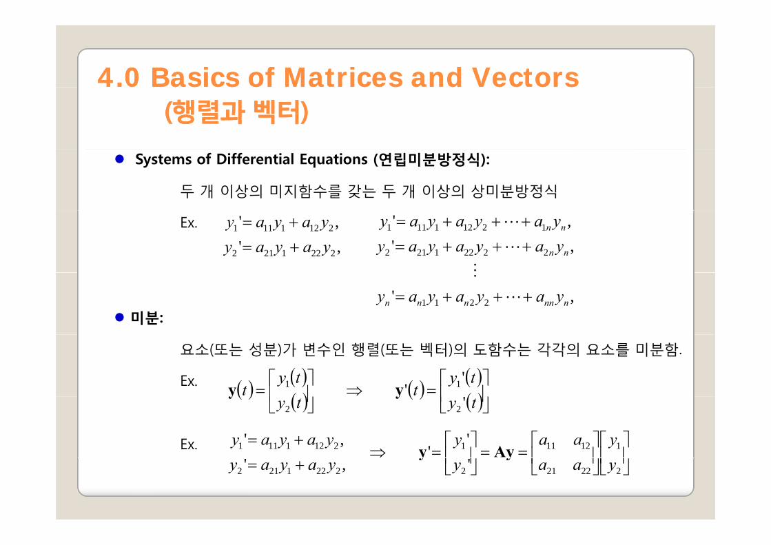
Systems of Differential Equations (연립미분방정식):

두 개 이상의 미지함수를 갖는 두 개 이상의 상미분방정식

Ex.

,','

2221212

2121111

yayayyayay

+=+=

,','

22221212

12121111

nn

nn

yayayayyayayay

+++=+++=

미분:,' 2211 nnnnnn yayayay +++=

요소(또는 성분)가 변수인 행렬(또는 벡터)의 도함수는 각각의 요소를 미분함.

Ex. ( ) ( )( ) ( ) ( )

( )⎥⎤

⎢⎡

=⇒⎥⎤

⎢⎡

=ty

tty

t'

' 11 yy

Ex.

( ) ( ) ( ) ( )⎥⎦⎢⎣

⎥⎦

⎢⎣ tyty '22

yy

⎥⎤

⎢⎡

⎥⎤

⎢⎡

==⎥⎤

⎢⎡

=⇒+= 1121112121111 '

' ,' yaayyayay

Ayy ⎥⎦

⎢⎣

⎥⎦

⎢⎣

⎥⎦

⎢⎣+= 2222122221212 ',' yaayyayay

yy


Eigenvalue (고유값) Eigenvector (고유벡터)Eigenvalue (고유값), Eigenvector (고유벡터)

[ ] 식 대하여 에 벡터 어떤 하고, 행렬이라 주어진 을 xAx0xA λ=≠×= nna jk

함. 라 대응하는

에 를 벡터 때의 이 하며, 이라 의 를 스칼라 하는 성립하게 가

or)(Eigenvect

xe)(Eigenvalu

고유벡터

고유값 λλ

해이다. 의 방정식 은 영벡터 대하여 에 임의의 xAx0x λλ ==

( )

연립방정식 1차 대수적인 관한 성분)에 의 벡터 미지수 개의 x

0xA0xAxxAx

(,, n

1 nxx

I

⇒

=−⇒=−⇒= λλλ

( ) 0det

=−⇔

−≠=

IA

IA0xxAx

λ

λλ

않는다. 하지

존재 역행렬이 의 계수행렬 위해서는 갖기 해를 인 이 방정식


Ex. 이면⎥⎦

⎤⎢⎣

⎡=

2221

1211

aaaa

A

( ) ( )( ) ( ) 2112221122112

211222112221

1211det aaaaaaaaaaaaaa

−++−=−−−=−

−=− λλλλ

λλ

λIA

( )2Characteristic Equation (특성방정식):

• 행렬 A의 고유값: 특성방정식의 해

• x가 행렬 A의 고유벡터이면 임의의 스칼라 에 대하여 도 고유벡터임

( ) 02112221122112 =−++− aaaaaa λλ

0≠k xk• x가 행렬 A의 고유벡터이면 임의의 스칼라 에 대하여 도 고유벡터임0≠k xk

Ex. 1 Eigenvalue Problem

Find the eigenvalue and eigenvectors of the matrixFind the eigenvalue and eigenvectors of the matrix

⎥⎦

⎤⎢⎣

⎡−=

21610.40.4

A ⎥⎦

⎢⎣− 2.16.1


Ex. 이면⎥⎦

⎤⎢⎣

⎡=

2221

1211

aaaa

A

( ) ( )( ) ( ) 2112221122112

211222112221

1211det aaaaaaaaaaaaaa

−++−=−−−=−

−=− λλλλ

λλ

λIA

( )2Characteristic Equation (특성방정식):

• 행렬 A의 고유값: 특성방정식의 해

• x가 행렬 A의 고유벡터이면 임의의 스칼라 에 대하여 도 고유벡터임

( ) 02112221122112 =−++− aaaaaa λλ

0≠k xk• x가 행렬 A의 고유벡터이면 임의의 스칼라 에 대하여 도 고유벡터임0≠k xk

Ex. 1 Eigenvalue Problem

Find the eigenvalue and eigenvectors of the matrixFind the eigenvalue and eigenvectors of the matrix

⎥⎦

⎤⎢⎣

⎡−=

21610.40.4

A ( ) ( )⎥⎦

⎤⎢⎣

⎡=⎥

⎦

⎤⎢⎣

⎡=−=−=

801

,12

8.0 ,2 2121 xxλλ⎥

⎦⎢⎣− 2.16.1 ⎥

⎦⎢⎣

⎥⎦

⎢⎣ 8.01


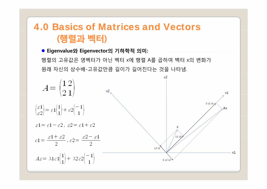
Eigenvalue와 Eigenvector의 기하학적 의미:Eigenvalue와 Eigenvector의 기하학적 의미:

행렬의 고유값은 영벡터가 아닌 벡터 x에 행렬 A를 곱하여 벡터 x의 변화가

원래 자신의 상수배-고유값만큼 길이가 길어진다는 것을 나타냄.

44.1 Systems of ODEs as Models.1 Systems of ODEs as ModelsSys e s o O s as ode sSys e s o O s as ode s((연립상미분방정식연립상미분방정식 모델모델))

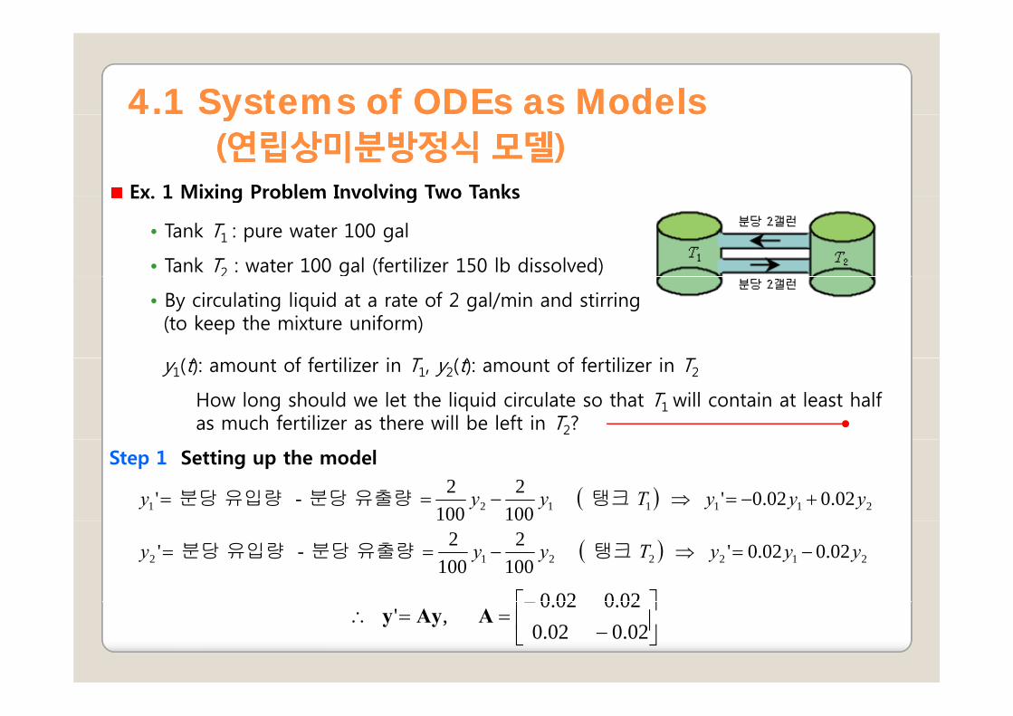
Ex 1 Mixing Problem Involving Two TanksEx. 1 Mixing Problem Involving Two Tanks

• Tank T1 : pure water 100 gal

• Tank T2 : water 100 gal (fertilizer 150 lb dissolved)

( ) f f ili i T ( ) f f ili i T

2

• By circulating liquid at a rate of 2 gal/min and stirring (to keep the mixture uniform)

y1(t): amount of fertilizer in T1, y2(t): amount of fertilizer in T2

How long should we let the liquid circulate so that T1 will contain at least half as much fertilizer as there will be left in T2?


Ex 1 Mixing Problem Involving Two TanksEx. 1 Mixing Problem Involving Two Tanks

• Tank T1 : pure water 100 gal

• Tank T2 : water 100 gal (fertilizer 150 lb dissolved)

( ) f f ili i T ( ) f f ili i T

2

• By circulating liquid at a rate of 2 gal/min and stirring (to keep the mixture uniform)

y1(t): amount of fertilizer in T1, y2(t): amount of fertilizer in T2

How long should we let the liquid circulate so that T1 will contain at least half as much fertilizer as there will be left in T2?

Step 1 Setting up the model

( ) 2111121 02.002.0' 100

2100

2 - ' yyyTyyy +−=⇒−== 탱크 유출량 분당 유입량 분당

( ) 2122212 02.002.0' 100

2100

2 - ' yyyTyyy −=⇒−== 탱크 유출량 분당 유입량 분당

⎤⎡− 020020⎥⎦

⎤⎢⎣

⎡−

−==∴

02.002.002.002.0

,' AAyy


andbothfor yye tλ

Step 2 General Solution

Idea: t 에 대한 지수함수로 시도 0)(')(''0)(')(''

221122211222112

121122211122111

=−++−=−++−

yaaaayaayyaaaayaay

21 andboth for yye

⇒=⇒==⇒= ' xAxAxxyxy λλ λλλ ttt eee 행렬 A의 고유값과 고유벡터 계산

특성방정식: 0)()( 2112221122112 =−++− aaaaaa λλ

( ) ( ) ( ) 004.002.002.002.002.002.002.0

det 22 =+=−−−=−−

−−=− λλλ

λλ

λIA

⎤⎡⎤⎡

0)()( 211222112211 ++ aaaaaa λλ

중첩의 원리 적용

( ) ( )⎥⎦

⎤⎢⎣

⎡−

=⎥⎦

⎤⎢⎣

⎡=−==⇒

11

,11

04.0 ,0 2121 xxλλ고유값 : 고유벡터 :

중첩의 원리 적용

( ) ( ) ( )상수 임의의 는과 1

111

1104.0

212

21

121 cceccecec ttt −

⎥⎦

⎤⎢⎣

⎡+⎥

⎦

⎤⎢⎣

⎡=+= λλ xxy

11 ⎥⎦

⎢⎣−⎥

⎦⎢⎣


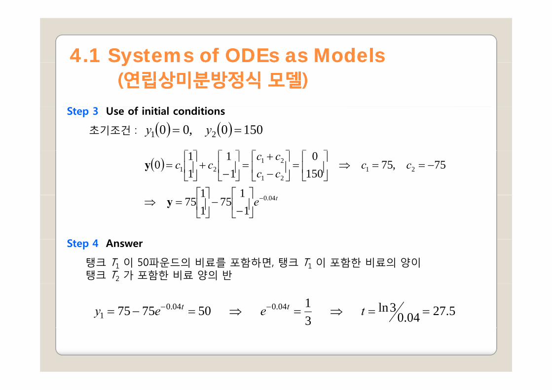
Step 3 Use of initial conditions

초기조건 : ( ) ( ) 1500 ,00 21 == yy

⎤⎡⎤⎡⎤⎡⎤⎡( ) cccccc

cc 2121

2121

11

75 ,75 150

01

111

0

⎤⎡⎤⎡

−==⇒⎥⎦

⎤⎢⎣

⎡=⎥

⎦

⎤⎢⎣

⎡−+

=⎥⎦

⎤⎢⎣

⎡−

+⎥⎦

⎤⎢⎣

⎡=y

S

te 04.0

11

7511

75 −⎥⎦

⎤⎢⎣

⎡−

−⎥⎦

⎤⎢⎣

⎡=⇒ y

Step 4 Answer

탱크 T1 이 50파운드의 비료를 포함하면, 탱크 T1 이 포함한 비료의 양이탱크 T2 가 포함한 비료 양의 반

5.2704.03ln

31 507575 04.004.0

1 ==⇒=⇒=−= −− teey tt


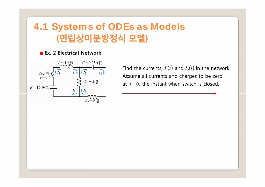
E 2 El i l N k

Find the currents, and in the network.

Ex. 2 Electrical Network

( )tI1 ( )tI2Assume all currents and charges to be zero

at , the instant when switch is closed. 0=t


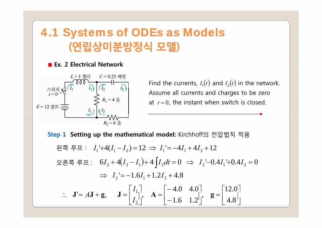
E 2 El i l N k

Find the currents, and in the network.

Ex. 2 Electrical Network

( )tI1 ( )tI2Assume all currents and charges to be zero

at , the instant when switch is closed. 0=t

Step 1 Setting up the mathematical model: Kirchhoff의 전압법칙 적용

왼쪽 루프 :

오른쪽 루프 :

1244' 12)(4' 211211 ++−=⇒=−+ IIIIII

( ) 04.0'4.0' 0446 2122122 =+−⇒=+−+ ∫ IIIdtIIII

⎤⎡⎤⎡−⎤⎡ 0.120.40.41I

( )8.42.16.1' 212

2122122

++−=⇒∫III

⎥⎦

⎤⎢⎣

⎡=⎥

⎦

⎤⎢⎣

⎡−

=⎥⎦

⎤⎢⎣

⎡=+=∴

8.4 ,

2.16.1 , ,'

2

1 gAJgJJI

A


Step 2 General Solution

제차 연립방정식 에 를 대입하면 이므로JJ A=' teλxJ = xAx λ=

A의 고유값과 고유벡터 계산

고유값 일 때, 고유벡터 ;21 −=λ ( )⎥⎦

⎤⎢⎣

⎡=

121x

고유값 일 때, 고유벡터8.02 −=λ ( )⎥⎦

⎤⎢⎣

⎡=

8.012x

제차 연립미분방정식의 일반해 : tth ecec 8.0

22

1 8.01

12 −−

⎥⎦

⎤⎢⎣

⎡+⎥

⎦

⎤⎢⎣

⎡=J


비제차 연립미분방정식의 특수해 구하기

라 하면, 이므로⎥⎦

⎤⎢⎣

⎡= 1a

pJ ⎥⎦

⎤⎢⎣

⎡=

00

'pJ 0g =+⎥⎦

⎤⎢⎣

⎡ 1aA

일반해 :

⎥⎦

⎢⎣ 2a

p ⎥⎦

⎢⎣0p ⎥

⎦⎢⎣ 2a

⎥⎤

⎢⎡

=∴==⇒=++−

⇒3

0300.120.40.4 21 aa

aaJ ⎥

⎦⎢⎣

=∴==⇒=++−

⇒0

0 ,3 08.42.16.1

2121

paaaa

J

tttt ececI 8.0

22

11802 32312 −− ++=⎤⎡⎤⎡⎤⎡tt

tt

ececIececIecec 8.0

22

12

2118.02

21 8.0

32 08.01 −−

−−

+=++

⇒⎥⎦

⎤⎢⎣

⎡+⎥

⎦

⎤⎢⎣

⎡+⎥

⎦

⎤⎢⎣

⎡=J

초기조건 적용

( ) tt eeIcc

ccI 8.021211 358

540320 −− ++−=

∴==⇒=++=

( ) tt eeIcc

ccI 8.022

21212 44

5 ,4 08.00 −− +−=

∴=−=⇒=+=


• 그림 79a는 과 의 곡선을 개별적으로 나타낸 것( )tI1 ( )tI2• 그림 79b는 평면에서 하나의 곡선 을

그린 것 ⇒ t 를 parameter(매개변수)로 하는 매개변수표현식

( )1 ( )2

−21II ( ) ( )[ ]tItI 21 ,

• 평면을 방정식 의 phase plane

(상평면)이라 함

−21II ( ) 0xIA =− λ

• 상편면에서의 곡선을 Trajectory(궤적)라 한다.

• 상평면의 궤적이 전체 해집합의 일반적인 양상을

잘 표현할 수 있음잘 표현할 수 있음


Conversion of an n th-Order ODE to a System

• n 계 상미분방정식: ( ) ( )( )1' −= nn yyytFyn 계 상미분방정식:

• 1계 연립상미분방정식으로의 변환

( ),,,, yyytFy

yyyy

''

32

21

==

( )

nn

nn

yy

yyyyyyyyyy

' ,,'' ,' ,

1

321

321

=⇒==== −

( )nn

nn

yyytFyyy

,,,,' 21

1

=−


Ex. 3 Mass on a Spring

앞에서 다룬 용수철에 달린 물체의 자유진동을 모델화하는 문제에 변환방법을 적용

0''' =++ kycymy212

21

'

'

ycyky

yy

−−=

=' , 21 yyyy ==

212 ym

ym

y

⎥⎦

⎤⎢⎣

⎡=

2

1

yy

y⎤⎡⎤⎡ 10⎦⎣ 2y

⎥⎦

⎤⎢⎣

⎡

⎥⎥⎦

⎤

⎢⎢⎣

⎡−−==

2

110

'yy

mc

mkAyy

( ) ⇒=++=−−−

−=− 0

1det 2

mk

mc

mc

mk λλλλ

λIA 2.4 절의 특성방정식과 일치mm


m = 1, c = 2, and k = 0.75


m = 1, c = 2, and k = 0.75

고유값 일 때, 고유벡터 ;5.01 −=λ ( )⎥⎦

⎤⎢⎣

⎡−

=1

21x

고유값 일 때, 고유벡터5.12 −=λ ( )⎥⎦

⎤⎢⎣

⎡−

=5.1

12x

제차 연립미분방정식의 일반해 : tt ececy 5.12

5.01 51

11

2 −−⎥⎦

⎤⎢⎣

⎡−

+⎥⎦

⎤⎢⎣

⎡−

=5.11 ⎦⎣−⎦⎣−


PROBLEM SET 4.1

HW 16HW: 16

44.2 Basic Theory of Systems of ODEs .2 Basic Theory of Systems of ODEs as c eo y o Sys e s o O sas c eo y o Sys e s o O s((연립상미분방정식에연립상미분방정식에 대한대한 기본기본 이론이론))

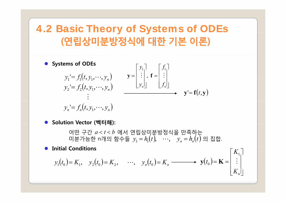
Systems of ODEs

( )yytfy ' 111 = ⎥⎥⎤

⎢⎢⎡

=⎥⎥⎤

⎢⎢⎡

=fy 11

, fy( )( )n

n

yytfyyytfy

,,,',,,

122

111

= ⎥⎥⎦⎢

⎢⎣⎥

⎥⎦⎢

⎢⎣ nn fy

,y

( )yfy ,' t=

Solution Vector (벡터해):

( )nnn yytfy ,,,' 1=

Solution Vector (벡터해):

어떤 구간 에서 연립상미분방정식을 만족하는미분가능한 n개의 함수들 의 집합.

I iti l C diti

bta <<( ) ( )thythy nn == , ,11

Initial Conditions

( ) ( ) ( ) nn KtyKtyKty === 0202101 , , , ( )⎥⎥⎥

⎦

⎤

⎢⎢⎢

⎣

⎡==K

Kt

1

0 Ky⎥⎦⎢⎣ nK


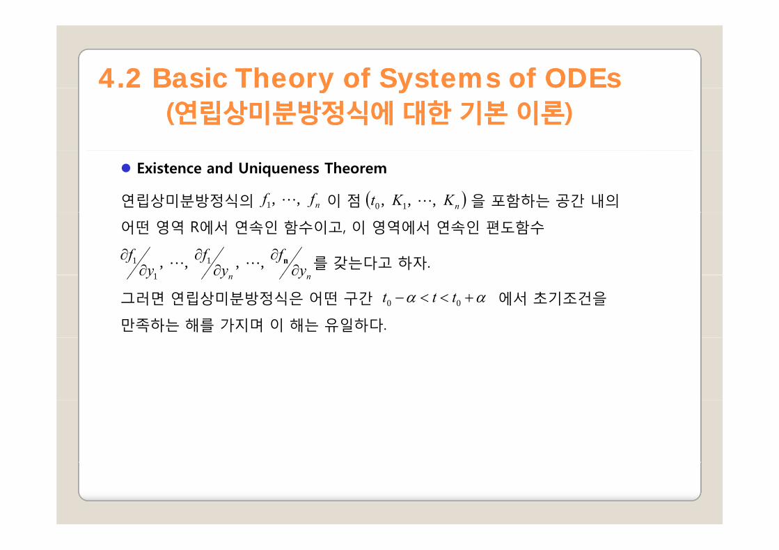
Existence and Uniqueness Theorem

연립상미분방정식의 이 점 을 포함하는 공간 내의nff , ,1 ( )nKKt , , , 10

어떤 영역 R에서 연속인 함수이고, 이 영역에서 연속인 편도함수

를 갖는다고 하자. yf

yf

yf

∂∂

∂∂

∂∂ n , , , , 1

1

1

그러면 연립상미분방정식은 어떤 구간 에서 초기조건을

만족하는 해를 가지며 이 해는 유일하다.

nn yyy ∂∂∂ 1

αα +<<− 00 ttt


Linear System

⎥⎥⎤

⎢⎢⎡

⎥⎥⎤

⎢⎢⎡

⎥⎥⎤

⎢⎢⎡ n gyaa 11111

gyA( ) ( ) ( )

( ) ( ) ( )ttt

tgytaytay nn

+++

+++= 111111

'

'gAyy +='

⎥⎥⎥

⎦⎢⎢⎢

⎣

=⎥⎥⎥

⎦⎢⎢⎢

⎣

=⎥⎥⎥

⎦⎢⎢⎢

⎣

=

nnnnn gyaa 1

, , gyA

Homogeneous:

( ) ( ) ( )tgytaytay nnnnnn +++= 11'

Ayy ='

Nonhomogeneous: 0ggAyy ≠+= ,'


Existence and Uniqueness in the Linear Case

선형연립미분방정식의 와 가 점 를 포함하는 열린 구간 내에서a jg tt = βα << t선형연립미분방정식의 와 가 점 를 포함하는 열린 구간 내에서

t 의 연속함수라 하자. 그러면 선형연립미분방정식은 이 구간에서 초기조건을

만족하는 해를 가지며 이 해는 유일하다

jka jg 0tt = βα << t

만족하는 해를 가지며 이 해는 유일하다.

Superposition Principle or Linearity Principle p p p y p

과 가 어떤 주어진 구간에서 제차선형연립방정식의 해이면,

그들의 일차 결합 또한 제차선형연립방정식의 해이다.

( )1y ( )2y( ) ( )2

21

1 yyy cc +=들의 일차 결합 한 제차선형연립방정식의 해이다21 yyy


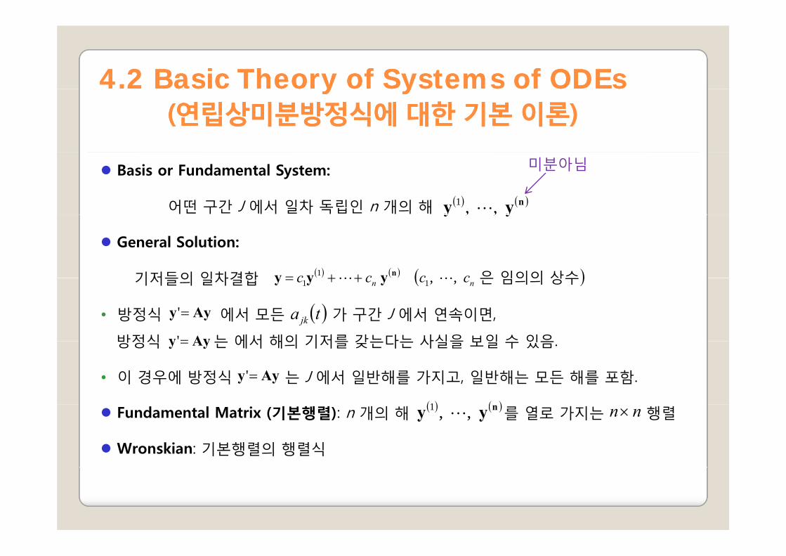
Basis or Fundamental System:

어떤 구간 J 에서 일차 독립인 n 개의 해 ( ) ( )nyy , ,1

미분아님

General Solution:

기저들의 일차결합

yy ,,

( ) ( ) ( )1 cccc nyyy ++= 은 임의의 상수기저들의 일차결합

• 방정식 에서 모든 가 구간 J 에서 연속이면,

방정식 는 에서 해의 기저를 갖는다는 사실을 보일 수 있음

( ) , , 11 nn cccc yyy ++= 은 임의의 상수

Ayy =' ( )ta jkAyy ='방정식 는 에서 해의 기저를 갖는다는 사실을 보일 수 있음.

• 이 경우에 방정식 는 J 에서 일반해를 가지고, 일반해는 모든 해를 포함.

Ayy =

Ayy ='

( ) ( )1Fundamental Matrix (기본행렬): n 개의 해 를 열로 가지는 행렬

Wronskian: 기본행렬의 행렬식

( ) ( )nyy , ,1 nn×


)()2()1(

)(1

)2(1

)1(1

n

nyyy)(

2)2(

2)1(

2)()1(

),,(n

n yyyyyW =

)()2()1( nnnn yyy

yy

Cf) Section 2.6

( )''

,21

2121 yy

yyyyW =

44.3 Constant.3 Constant--CoefficientCoefficient Systems.Systems.Ph Pl M th dPh Pl M th dPhase Plane MethodPhase Plane Method((상수계수를상수계수를 갖는갖는 연립방정식연립방정식. . 상평면법상평면법))

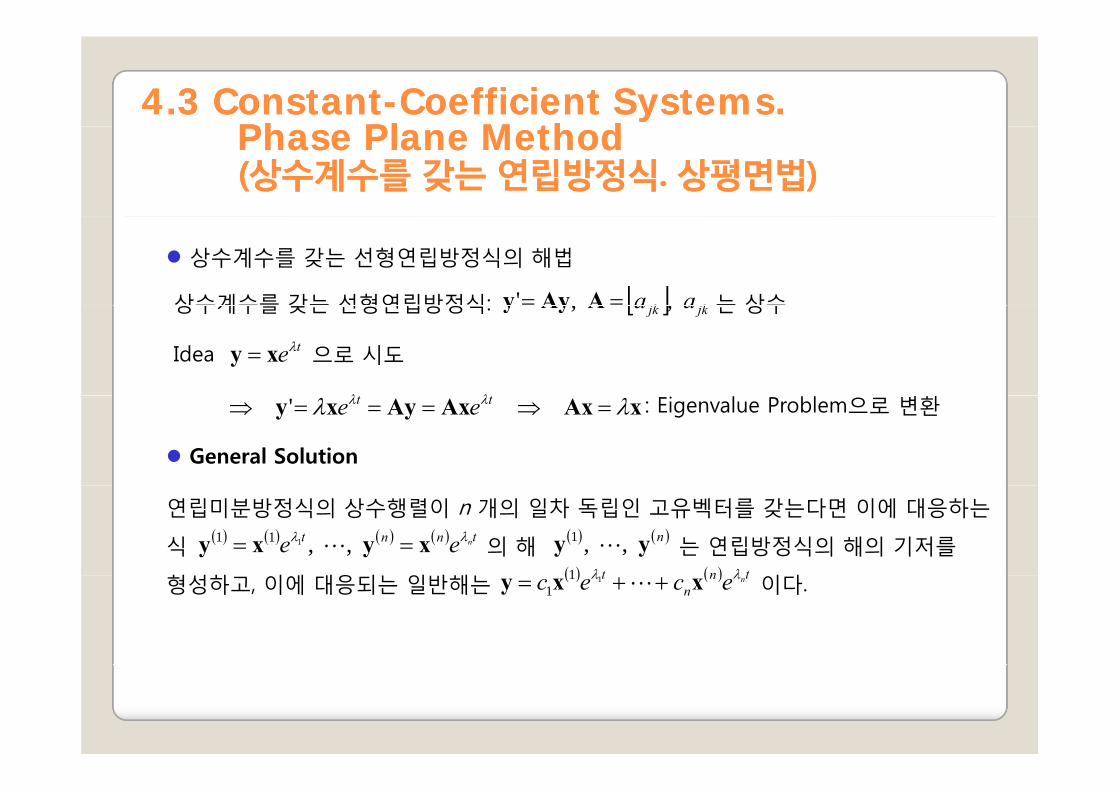
상수계수를 갖는 선형연립방정식의 해법

상수계수를 갖는 선형연립방정식: 는 상수[ ] jkjk aa ,,' == AAyy상수계수를 갖는 선형연립방정식: 는 상수

Idea 으로 시도

[ ] jkjk aa , , AAyy

teλxy =

λλ : Eigenvalue Problem으로 변환

General Solution

xAxAxAyxy λλ λλ =⇒===⇒ ' tt ee

연립미분방정식의 상수행렬이 n 개의 일차 독립인 고유벡터를 갖는다면 이에 대응하는

식 의 해 는 연립방정식의 해의 기저를

형성하 이에 대응되 일반해 이다

( ) ( ) ( ) ( ) tnnt nee λλ xyxy == , ,111 ( ) ( )nyy , ,1

( ) ( ) tnt λλ1형성하고, 이에 대응되는 일반해는 이다. ( ) ( ) tnn

t necec λλ xxy ++= 111


How to Graph Solutions in the Phase Plane

의 일반해⎟⎟⎞

⎜⎜⎛ +=⇔= 2121111' '

yayayAyy

( )( )⎥

⎤⎢⎡

=ty1y

• 성분 와 를 t -축 위에 두 개의 곡선으로 나타냄.

⎟⎠

⎜⎝ += 2221212 ' yayay

yy ( )⎥⎦⎢⎣ ty2

y

( )ty1 ( )ty1

• 매개변수 t 를 사용한 매개변수표현법 (또는, 매개변수방정식):

평면에 하나의 곡선으로 나타낼 수 있음−21 yy 평면에 하나의 곡선으로 나타낼 수 있음.

용어정리

21 yy

• Trajectory (궤적), 때로는 Orbit (궤도), Path (경로): 평면의 곡선

• Phase Plane (상평면): 평면

−21 yy

−21 yy

• Phase Portrait (상투영): 상평면을 방정식 의 궤적들로 채워서 얻는다.Ayy ='


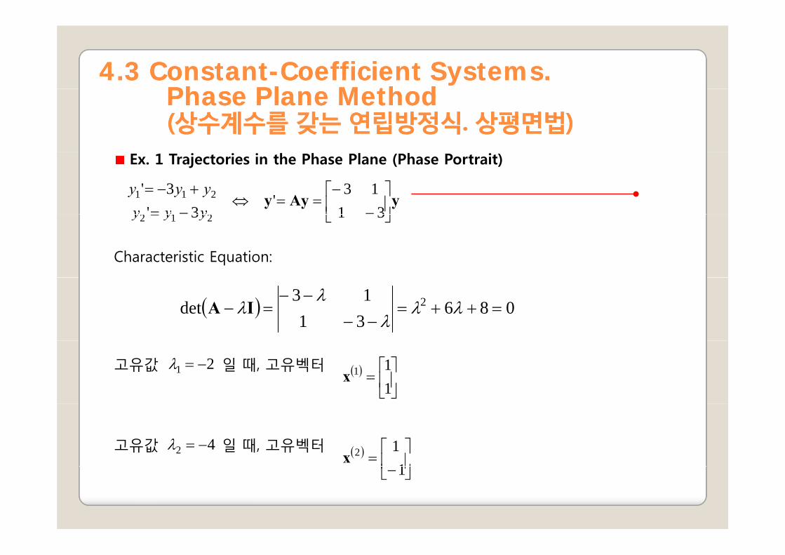
Ex. 1 Trajectories in the Phase Plane (Phase Portrait)

yAyy ⎥⎦

⎤⎢⎣

⎡−

−==⇔

−=+−=

3113

' 3'

3'

212

211

yyyyyy

Characteristic Equation:

⎦⎣= 313 212 yyy

( ) 0863113

det 2 =++=−−

−−=− λλ

λλ

λIA

고유값 일 때, 고유벡터21 −=λ ( )⎥⎦

⎤⎢⎣

⎡=

111x

고유값 일 때, 고유벡터42 −=λ ( )⎥⎦

⎤⎢⎣

⎡=

112x ⎥

⎦⎢⎣−1


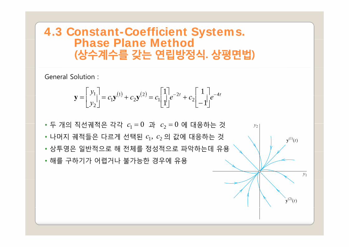
General Solution :

( ) ( ) tty 42211 11 −−⎥⎤

⎢⎡

+⎥⎤

⎢⎡

+⎥⎤

⎢⎡

두 개의 직선궤적은 각각 과 에 대응하는 것

( ) ( ) tt ececccy

42

21

22

11

2

1

11 ⎥⎦

⎢⎣−

+⎥⎦

⎢⎣

=+=⎥⎦

⎢⎣

= yyy

0c 0c• 두 개의 직선궤적은 각각 과 에 대응하는 것

• 나머지 궤적들은 다르게 선택된 의 값에 대응하는 것

• 상투영은 일반적으로 해 전체를 정성적으로 파악하는데 유용

01 =c 02 =c

21 , cc상투영은 일반적 해 전체를 정성적 파악하는데 유용

• 해를 구하기가 어렵거나 불가능한 경우에 유용


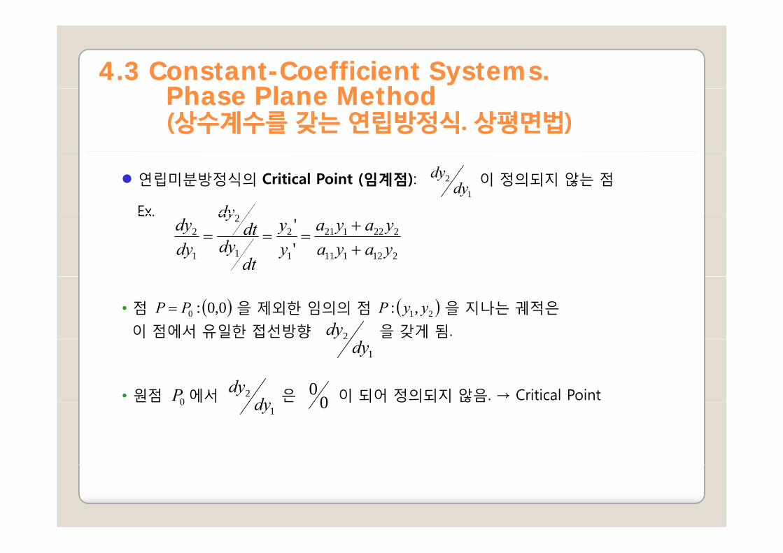
연립미분방정식의 Critical Point (임계점): 이 정의되지 않는 점

Ex1

2dy

dy

dyEx.

212111

222121

1

2

1

2

1

2

''

yayayaya

yy

dtdydt

dy

dydy

++

===

• 점 을 제외한 임의의 점 을 지나는 궤적은

이 점에서 유일한 접선방향 을 갖게 됨.

( )0,0:0PP = ( )21,: yyP

2dy

• 원점 에서 은 이 되어 정의되지 않음. → Critical Point

1dy

0P 2d

dy0

0원점 에서 은 이 되어 정의되지 않음01dy 0


Five Types of Critical Points:

형임계점은 근방에서 궤적의 모양에 따라 5가지 유형으로 구분.

Improper Node (비고유마디점)• Improper Node (비고유마디점)

• Proper Node (고유마디점)

• Saddle Point (안장점)( 장 )

• Center (중심점)

• Spiral Point (나선점)


E 1 I N dEx. 1 Improper Node:

두 개의 궤적을 제외한 모든 궤적이 주어진 점에서 같은 접선방향의 극한을 갖는 경우.

• 예외적인 두 개의 궤적도 주어진 점에서 접선방향의 극한을 갖게 됨

• 극한값은 앞의 극한값과 다르다.

yAyy ⎥⎦

⎤⎢⎣

⎡−

−==

3113

'

⎤⎡1• 공통인 접선방향이 극한은 고유벡터 임.

( )⎥⎦

⎤⎢⎣

⎡=

111x

(t 가 증가할 때 가 보다 훨씬 더 빨리 0에 접근)

• 예외적인 궤적의 접선방향극한: ,

te 4− te 2−

( )⎥⎤

⎢⎡

=12x ( )

⎥⎤

⎢⎡−

=−12x예외적인 궤적의 접선방향극한: ,⎥

⎦⎢⎣−1

x ⎥⎦

⎢⎣ 1


Ex. 2 Proper Node :

모든 궤적이 명확한 접선방향의 극한을 가지고, 임의로 주어진 방향 d에 대하여 d를 극한방향으로 가지는 궤적이 존재하는 경우임의로 주어진 방향 d에 대하여 d를 극한방향으로 가지는 궤적이 존재하는 경우.

⎟⎟⎞

⎜⎜⎛ =

⎥⎤

⎢⎡

= 11' ,

01'

yy즉,yy

G l S l i

⎟⎟⎠

⎜⎜⎝ =⎥

⎦⎢⎣ 22 '

,10 yy

즉,yy

General Solution:

22

1121

10

01

ecyecyecec t

ttt

==

⇒⎥⎦

⎤⎢⎣

⎡+⎥

⎦

⎤⎢⎣

⎡=y

1221

22

ycyc

y

=⇒

⎦⎣⎦⎣

1221 ycyc =⇒


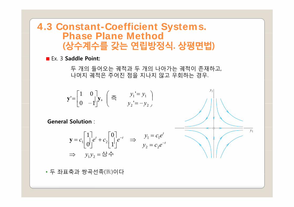
E 3 S ddl P iEx. 3 Saddle Point:

두 개의 들어오는 궤적과 두 개의 나아가는 궤적이 존재하고, 나머지 궤적은 주어진 점을 지나지 않고 우회하는 경우.

⎟⎟⎠

⎞⎜⎜⎝

⎛−=

=⎥⎦

⎤⎢⎣

⎡−

= 11

''

,10

01'

yyyy

즉yy

General Solution :

⎠⎝ =⎦⎣ 2210 yy

==

⇒⎥⎦

⎤⎢⎣

⎡+⎥

⎦

⎤⎢⎣

⎡=

−−

22

1121

10

01

ecyecy

ecec t

ttty

• 두 좌표축과 쌍곡선족(族)이다

상수=⇒ 21 yy

두 좌 축과 쌍곡선족( )이다


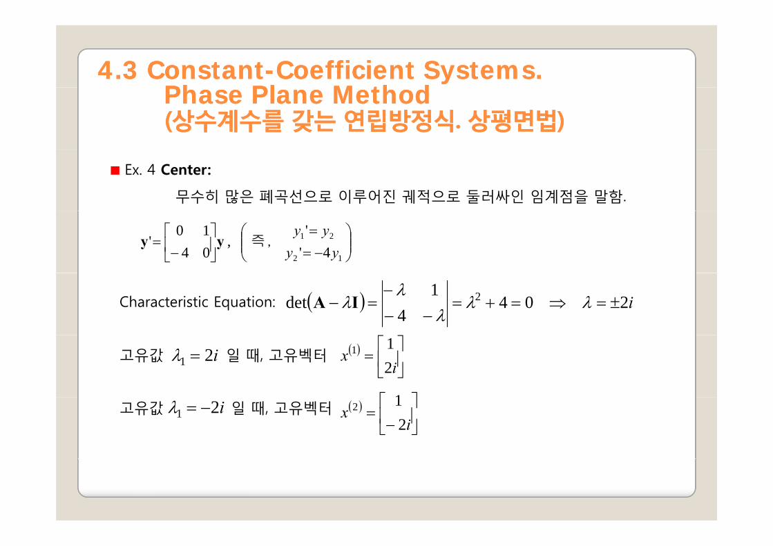
Ex. 4 Center:

무수히 많은 폐곡선으로 이루어진 궤적으로 둘러싸인 임계점을 말함.

⎟⎟⎠

⎞⎜⎜⎝

⎛−=

=⎥⎦

⎤⎢⎣

⎡−

=12

21

4''

, 0410

'yyyy

즉,yy

Characteristic Equation: ( ) i2 044

1det 2 ±=⇒=+=

−−−

=− λλλ

λλIA

고유값 일 때, 고유벡터i21 =λ ( )⎥⎦

⎤⎢⎣

⎡=

ix

211

⎤⎡ 1고유값 일 때, 고유벡터i21 −=λ ( )⎥⎦

⎤⎢⎣

⎡−

=i

x212


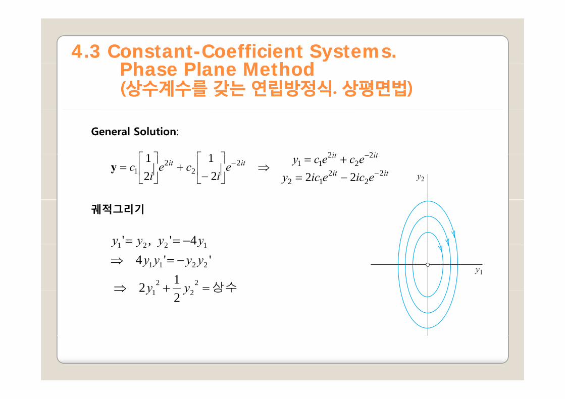
General Solution:

itit 2211 ⎤⎡⎤⎡itit

itititit

eiceicyececye

ice

ic 2

22

12

22

2112

22

1 22

21

21

−

−−

−=+=

⇒⎥⎦

⎤⎢⎣

⎡−

+⎥⎦

⎤⎢⎣

⎡=y

궤적그리기

−== 1221 4' ,' yyyy

상수=+⇒

−=⇒

22

21

2211

1221

12

''4 ,

yy

yyyyyyyy

상수+⇒ 21 22 yy


E 5 S i l P iEx. 5 Spiral Point:

를 취할 때, 임계점 근방에서 나선형의 궤적이 임계점으로 향하여 접근하는(혹은 임계점로부터 벗어나 멀어지는) 경우.

∞→t

⎟⎟⎠

⎞⎜⎜⎝

⎛−−=+−=

⎥⎦

⎤⎢⎣

⎡−−

−=

212

211

''

, 11

11'

yyyyyy

즉yy

특성방정식:

⎤⎡

( ) i±−=⇒=++=−−−

−−=− 1 022

1111

det 2 λλλλ

λλIA

고유값 일 때, 고유벡터i+−= 11λ ( )⎥⎦

⎤⎢⎣

⎡=i

x11

( ) ⎤⎡ 1고유값 일 때, 고유벡터

일반해 ( ) ( )titi −−+−⎥⎤

⎢⎡

+⎥⎤

⎢⎡ 11 11

i−−= 11λ ( )⎥⎦

⎤⎢⎣

⎡−

=i

x12

일반해 : ( ) ( )titi ei

cei

c +⎥⎦

⎢⎣−

+⎥⎦

⎢⎣

= 12

11y


궤적그리기

극좌표 이용

( )( )2

22

12211

212211

''

' ,'

yyyyyy

yyyyyy

+−=+⇒

−−=+−= 22

21

2 yyr += ( ) 22 ' 21 rr −=

( ) '2' 2 rrr =2' rrr −=

변수분리형 해법에 의하여 적분하면

tcerctr −=⇒+−= *ln


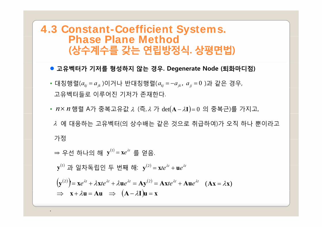
고유벡터가 기저를 형성하지 않는 경우. Degenerate Node (퇴화마디점)

• 대칭행렬( )이거나 반대칭행렬( )과 같은 경우,jkkj aa = 0 , =−= jjjkkj aaa

고유벡터들로 이루어진 기저가 존재한다.

• 행렬 A가 중복고유값 (즉, 가 의 중복근)를 가지고, nn× λ λ ( ) 0det =− IA λ

에 대응하는 고유벡터(의 상수배는 같은 것으로 취급하여)가 오직 하나 뿐이라고

가정

λ

가정

⇒ 우선 하나의 해 를 얻음.

과 일차독립인 두 번째 해

( ) teλxy =1

( )1 ( ) tt λλ2과 일차독립인 두 번째 해: ( )1y ( ) tt ete λλ uxy +=2

( )( ) ( )

( )AuAxAyuxxy +==++=

λλλλ λλλλλ ' 22 ttttt eteetee )( xAx λ=

.

( ) xuIAAuux =−⇒=+⇒ λλ


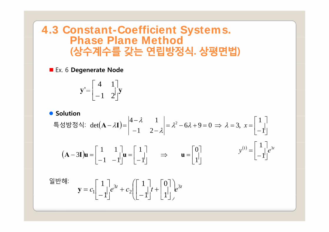
Ex. 6 Degenerate Node

yy ⎥⎤

⎢⎡

=14

' yy ⎥⎦

⎢⎣−

=21


Ex. 6 Degenerate Node

yy ⎥⎤

⎢⎡

=14

'

Solution

yy ⎥⎦

⎢⎣−

=21

특성방정식:

⎤⎡

( ) ⎥⎦

⎤⎢⎣

⎡−

==⇒=+−=−−

−=−

11

,3 09621

14det 2 xλλλ

λλ

λIA

( ) tey 31

11

⎥⎦

⎤⎢⎣

⎡−

=( ) ⎥⎦

⎤⎢⎣

⎡=⇒⎥

⎦

⎤⎢⎣

⎡−

=⎥⎦

⎤⎢⎣

⎡−−

=−10

1

111

113 uuuIΑ

일반해:tt etcec 3

23

1 10

11

11

⎟⎟⎠

⎞⎜⎜⎝

⎛⎥⎦

⎤⎢⎣

⎡+⎥

⎦

⎤⎢⎣

⎡+⎥

⎦

⎤⎢⎣

⎡=y

111 ⎟⎠

⎜⎝ ⎦⎣⎦⎣−⎦⎣−


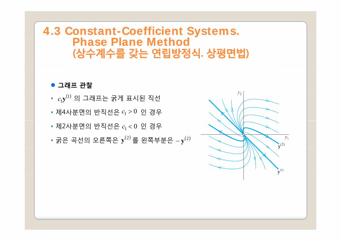
그래프 관찰

• 의 그래프는 굵게 표시된 직선

• 제4사분면의 반직선은 인 경우

( )11yc

01 >c

• 제2사분면의 반직선은 인 경우

• 굵은 곡선의 오른쪽은 를 왼쪽부분은

01 <c( )2y ( )2y−


PROBLEM SET 4.3

HW 9HW: 9

44.4 .4 Criteria for Critical Points. StabilityCriteria for Critical Points. StabilityC e a o C ca o s S a yC e a o C ca o s S a y((임계점에임계점에 대한대한 판별기준판별기준. . 안정성안정성))

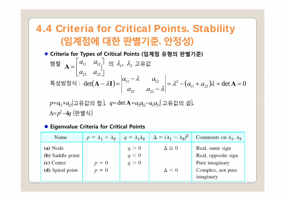
Criteria for Types of Critical Points (임계점 유형의 판별기준)Criteria for Types of Critical Points (임계점 유형의 판별기준)

행렬 의 고유값⎥⎦

⎤⎢⎣

⎡=

2221

1211

aaaa

A 21 , λλ

λ aa특성방정식 : ( ) ( ) 0detdet 2211

2

2221

1211 =++−=−

−=− AIA λλ

λλ

λ aaaaaa

( ) ( )d A( ) ( )( ) 4

, det , 2

211222112211

qp

aaaaqaap

−=Δ

−==+= A고유값의 합 고유값의 곱

판별식

Eigenvalue Criteria for Critical Points


Stability (안정성)Stability (안정성)

• 임계점의 또 다른 분류방식은 안정성에 의한 것

• 안정성은 물리학에서 처음 생각한 개념으로, 공학이나 응용 등 여러 분야에서

기본적인 개념

• 안정성은 어떤 순간에 물리적 계에 가해진 작은 변화(작은 충격)가 이후의 모든

시간 t 에서 계의 움직임에 단지 작은 영향을 미치는 것을 의미함.

Stable Critical point (안정적 임계점):

어떤 순간 에서 임계점에 아주 가깝게 접근한 모든 궤적이 이후의시간에서도 임계점에 아주 가까이 접근한 상태로 남아 있는 경우.

Unstable Critical point (불안정적 임계점): 안정적이 아닌 임계점

0tt =

Unstable Critical point (불안정적 임계점): 안정적이 아닌 임계점

Stable and Attractive Critical point (안정적 흡인 임계점):

안정적 임계점이고, 임계점 근처 원판 내부의 한 점을 지나는 모든 궤적이

를 취할 때 임계점에 가까이 접근하는 경우∞→t


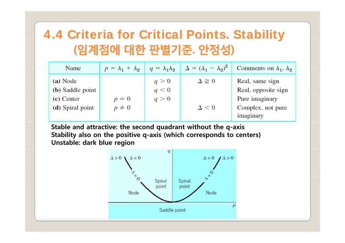
Stability Criteria for Critical PointsStability Criteria for Critical Points

Stability chart of the systemy yStable and attractive: the second quadrant without the q-axisStability also on the positive q-axis (which corresponds to centers)Unstable: dark blue region


Ex. 2 Free Motions of a Mass on a Spring

What kind of critical point does have?0''' =++ kycymy

No damping:

U d d iUnder damping:

Critical damping:

Overdamping:Overdamping:


Ex. 2 Free Motions of a Mass on a Spring

What kind of critical point does have?0''' =++ kycymy

yy ⎥⎦

⎤⎢⎣

⎡−−

=mcmk //

10'

( ) 0//1

det 2 =++=−−−

−=−

mk

mc

mcmkλλ

λλ

λIA

No damping: c = 0, p = 0, q > 0, a center

U d d i 2 4 k 0 0 0 bl d i i l i

// mmmcmk λ

Under damping: c2 < 4mk, p < 0, q > 0, Δ < 0, a stable and attractive spiral point

Critical damping: c2 = 4mk, p < 0, q > 0, Δ = 0, a stable and attractive node

Overdamping: c2 > 4mk, p < 0, q > 0, Δ > 0, a stable and attractive nodeOverdamping: c > 4mk, p < 0, q > 0, Δ > 0, a stable and attractive node


PROBLEM SET 4.4

HW 16HW: 16

44.5 .5 Qualitative Methods for NonlinearQualitative Methods for Nonlinear55 Qua a e e ods o o eaQua a e e ods o o eaSystems Systems ((비선형연립방정식에비선형연립방정식에 대한대한 정성법정성법))

Q lit ti M th d (정성법)Qualitative Method (정성법)

• 방정식의 해를 실제로 구하지 않으면서 해에 대한 정성적인 정보를 얻는 방법

• 연립방정식의 해를 해석적으로 구하기 어렵거나 불가능한 경우에 매우 유용한 방법

• 상평면법을 선형연립방정식으로부터 비선형연립방정식으로 확장


( ) ,' =

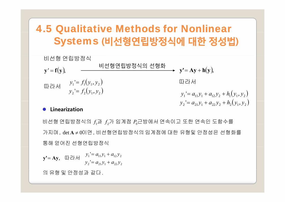
연립방정식 비선형

yfy ( ) ,+= yhAyy'비선형연립방정식의 선형화

( )( )2122

2111

,','

yyfyyyfy

==

따라서( )( )

2112121111

','

hyyhyayay ++=

따라서

( )2122221212 ,' yyhyayay ++=Linearization

도함수를연속인또한연속이고 근방에서임계점가과연립방정식의비선형 021 Pff

선형연립방정식 얻어진 통해

선형화를 안정성은 유형및 대한 임계점에 비선형연립방정식의 이면, 가지며,

021

0det

ff

≠A

따라서2221212

2121111

''

,yayayyayay

+=+=

= Ayy'

같다. 안정성과 및 유형 의


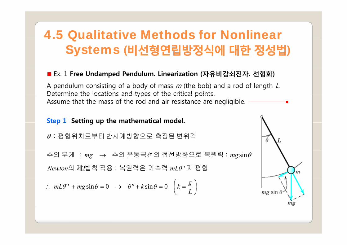
Ex. 1 Free Undamped Pendulum. Linearization (자유비감쇠진자. 선형화)

A pendulum consisting of a body of mass m (the bob) and a rod of length L. Determine the locations and types of the critical pointsDetermine the locations and types of the critical points. Assume that the mass of the rod and air resistance are negligible.

Step 1 Setting up the mathematical model.Step 1 Setting up the mathematical model.

변위각 측정된 반시계방향으로 평형위치로부터 : θ

→

mLθNewton

mgmg

''2

sin θ

평형 과 가속력 복원력은 : 적용 법칙제 의

: 복원력 접선방향으로 운동곡선의 추의 : 무게 추의

⎟⎠⎞

⎜⎝⎛ ==+→=+∴

Lgkkθ''mgmLθ 0sin 0sin '' θθ


Step 2 Critical points , Linearization.( ) ( ) ( ) ,0,4 ,0,2 ,0,0 ππ ±±

치환로'θθ0sin =+ θkθ''

치환로 ' , 21 θθ == yy

12

21

sin''

ykyyy

−==

( ) 21000sin0 ±±=→== nnπyy :임계점 ( ) ,2 ,1 ,0 ,0 0sin ,0 12 ±±=→== n,nπyy :임계점

( ) 고려 을 임계점 00,

13

111 61sin yyyyMaclaurin ≈−+−= 급수

21'10 yy'

=⎥⎤

⎢⎡

== 따라서yAyy12 '

,0 kyyk −=⎥

⎦⎢⎣−

== 따라서yAyy

중심 안정한 : 유형 임계점 44 ,det ,0 22211 ⇒−=−=Δ====+= kqp

Lgkqaap AL


Step 3 Critical points Linearization( ) ( ) ( )05030 ±±±Step 3 Critical points , Linearization.( ) ( ) ( ) ,0,5 ,0,3 ,0, πππ ±±±

( ) 고려 을 임계점 0 ,π

0sin =+ θkθ''( ) 치환 로 '' , 21 θπθπθ =−=−= yy

( ) 13

1111 61sinsinsin yyyyy −≈+−+−=−=+= πθ

yAyy ⎥⎦

⎤⎢⎣

⎡==

010

k'

6

( ) ( ) 불안정한안장점 : 유형 임계점 44 ,0 ,0 2 ⇒=−=Δ<−== kqpkqp


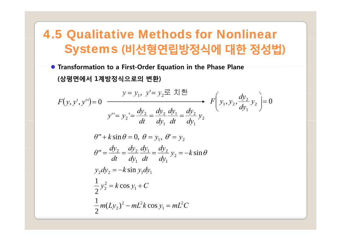
Transformation to a First Order Eq ation in the Phase PlaneTransformation to a First-Order Equation in the Phase Plane

(상평면에서 1계방정식으로의 변환)

치환로' yyyy == ⎞⎛( ) 0'',', =yyyF치환로21 , yyyy ==

22122

2 ''' ydydy

dtdy

dydy

dtdyyy ====

0,, 21

221 =⎟⎟

⎠

⎞⎜⎜⎝

⎛y

dydyyyF

11 dydtdydt

dydydydyy'ykθ'' 21 , ,0sin ===+ θθθ

dyykdyy

kydydy

dtdy

dydy

dtdyθ''

1122

21

21

1

22

sin

sin

−=

−==== θ

k

Cyky

222

122

)(1

cos21

+=

CmLykmLLym 21

222 cos)(

21

=−


PROBLEM SET 4.5

HW 16HW: 16

44.6 .6 NonhomogeneousNonhomogeneous Linear Systems Linear Systems 66 o o oge eouso o oge eous ea Sys e sea Sys e sof ODEs of ODEs ((비비제차제차 선형연립방정식선형연립방정식))

−t

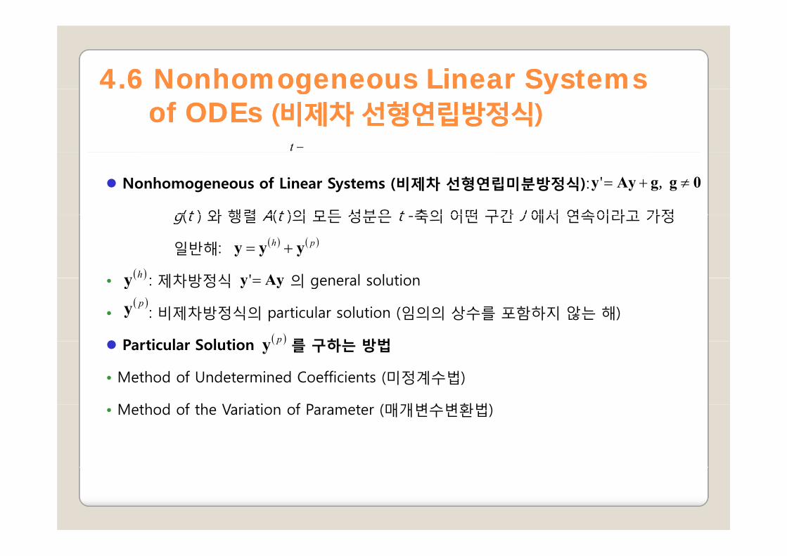
Nonhomogeneous of Linear Systems (비제차 선형연립미분방정식):

g(t ) 와 행렬 A(t )의 모든 성분은 t 축의 어떤 구간 J 에서 연속이라고 가정

0ggAyy ≠+= ,'

g(t ) 와 행렬 A(t )의 모든 성분은 t -축의 어떤 구간 J 에서 연속이라고 가정

일반해:

: 제차방정식 의 general solution

( ) ( )ph yyy +=( )hy Ayy'• : 제차방정식 의 general solution

• : 비제차방정식의 particular solution (임의의 상수를 포함하지 않는 해)

P ti l S l ti 를 구하는 방법

( )y( )py

Ayy ='

( )pParticular Solution 를 구하는 방법

• Method of Undetermined Coefficients (미정계수법)

M h d f h V i i f P (매개변수변환법)

( )py

• Method of the Variation of Parameter (매개변수변환법)


미정계수법: 벡터 g 의 성분이 t 의 거듭제곱 지수함수 사인함수와 코사인함수

Ex. 1 Find a general solution of

미정계수법: 벡터 g 의 성분이 t 의 거듭제곱, 지수함수, 사인함수와 코사인함수

등으로 이루어져 있을 때 적합.

g

tey 2

26

3113

' −⎥⎦

⎤⎢⎣

⎡−+⎥

⎦

⎤⎢⎣

⎡−

−=+= gAyy

제차연립방정식의 일반해:

미정계수법에 의하여 비제차연립방정식의 특수해 구하기

( ) tth ecec 42

21 1

111 −−

⎥⎦

⎤⎢⎣

⎡−

+⎥⎦

⎤⎢⎣

⎡=y

미정계수법에 의하여 비제차연립방정식의 특수해 구하기( ) ttp ete 22 −− += vuy ( )( ) gAvAuvuuy ++=−−= −−−−− tttttp eteetee 22222 22'

( )상수임의의::계수항의 aate t 122

⎥⎤

⎢⎡

=⇒=−− uAuu

( ) 선택 으로 : 계수 항의 0 4

,2 26

22 =⎥⎦

⎤⎢⎣

⎡+

=−=⇒⎥⎦

⎤⎢⎣

⎡−+=−− k

kk

ae t vAvvu

( )상수임의의:: 계수 항의 aate 1

2 ⎥⎦

⎢⎣

=⇒= uAuu

⎤⎡⎤⎡⎤⎡⎤⎡ tttt eteecec 2242

21 2

211

21

111 −−−−

⎥⎦

⎤⎢⎣

⎡−+⎥

⎦

⎤⎢⎣

⎡−⎥

⎦

⎤⎢⎣

⎡−

+⎥⎦

⎤⎢⎣

⎡=y일반해 :


매개변수변환법:

t -축의 어떤 구간 J 상에서 제차연립미분방정식의 일반해

를 이미 알고 있을 때, 이 일반해를 이용하여

방정식의 한 특수해를 찾아내는 방법

( ) ( ) ( )nn

h cc yyy ++= 11

( )제차연립방정식의 일반해:

비제차연립방정식의 특수해를 라 하자.

( ) ( ) ( )AYYcYy =∴= ' th

( ) ( ) ( )ttp uYy =

( )( )( ) ( )

t

p '' '''

∫

+=+⇒+= gAYuYuuYYuuYy

( ) ( ) tdttt

~~~ ' ' 0

11 ∫ −− =⇒=⇒=⇒ gYugYugYu


Ex 2 Solve Ex 1 by the method of variation of parametersEx. 2 Solve Ex. 1 by the method of variation of parameters.

( ) ( )cYy tcc

eeee

tt

tth =⎥

⎦

⎤⎢⎣

⎡⎥⎦

⎤⎢⎣

⎡

−=

−−

−−

2

142

42

⎦⎣⎦⎣ 2

tt

tt

tt

tt

t eeee

eeee

e 44

22

22

44

61

21

21

−−

−−

−−

⎥⎦

⎤⎢⎣

⎡

−=⎥

⎦

⎤⎢⎣

⎡

−−−

−=Y

ttt

t

tt

tt

eeee

eeee

222

2

44

221

42

84

21

26

21'

−

−−

⎥⎦

⎤⎢⎣

⎡−

−=⎥

⎦

⎤⎢⎣

⎡−

−=⎥

⎦

⎤⎢⎣

⎡−⎥⎦

⎤⎢⎣

⎡

−== gYu

ttttt

t

t

t et

tde

42242

20

~2

2222222

222~

42

⎤⎡⎤⎡⎤⎡⎤⎡⎤⎡

⎥⎦

⎤⎢⎣

⎡+−

−=⎥

⎦

⎤⎢⎣

⎡−

−= ∫u

( ) ttttt

ttt

ttt

ttp ee

tt

eeteeete

et

eeee 42

422

422

242

42

22

2222

222222

222 −−

−−−

−−−

−−

−−

⎥⎦

⎤⎢⎣

⎡−

+⎥⎦

⎤⎢⎣

⎡+−−−

=⎥⎦

⎤⎢⎣

⎡

−+−+−−

=⎥⎦

⎤⎢⎣

⎡+−

−⎥⎦

⎤⎢⎣

⎡

−== Yuy

2111 ⎤⎡−⎤⎡⎤⎡⎤⎡ tttt eteececy 2242

21 2

211

21

111

−−−−⎥⎦

⎤⎢⎣

⎡−+⎥

⎦

⎤⎢⎣

⎡−⎥

⎦

⎤⎢⎣

⎡−

+⎥⎦

⎤⎢⎣

⎡=∴


PROBLEM SET 4.6

HW 19HW: 19

engineering mathematics iocw.snu.ac.kr/sites/default/files/note/5093.pdf · zsystems of...

Documents