engineering mathematics pocket book - zodmljohn_bird_bsc_(hons)__ceng... · engineering mathematics...
TRANSCRIPT

Engineering Mathematics Pocket Book
Fourth Edition
John Bird

This page intentionally left blank
Engineering Mathematics Pocket Book
Fourth edition
John Bird BSc(Hons), CEng, CSci, CMath, FIMA, FIET, MIEE, FIIE, FCollT
AMSTERDAM • BOSTON • HEIDELBERG • LONDON • NEW YORK • OXFORDPARIS • SAN DIEGO • SAN FRANCISCO • SINGAPORE • SYDNEY • TOKYO
Newnes is an imprint of Elsevier

Newnes is an imprint of ElsevierLinace House, Jordan Hill, Oxford OX2 8DP, UK30 Corporate Drive, Suite 400, Burlington, MA 01803, USA
First published as the Newnes Mathematics for Engineers Pocket Book 1983Reprinted 1988, 1990 (twice), 1991, 1992, 1993Second edition 1997Third edition as the Newnes Engineering Mathematics Pocket Book 2001Fourth edition as the Engineering Mathematics Pocket Book 2008
Copyright © 2008 John Bird, Published by Elsevier Ltd. All rights reserved
The right of John Bird to be identified as the author of this work has been asserted in accordance with the Copyright, Designs and Patents Act 1988
No part of this publication may be reproduced, stored in a retrieval system or transmitted in any form or by any means electronic, mechanical, photocopying, recording or otherwise without the prior written permission of the publisher
Permission may be sought directly from Elsevier’s Science & Technology Rights Department in Oxford, UK: phone (�44) (0) 1865 843830; fax (�44) (0) 1865 853333; email: [email protected]. Alternatively you can submit your request online by visiting the Elsevier website at http:elsevier.com/locate/permissions, and selecting Obtaining permission to use Elsevier material
NoticeNo responsibility is assumed by the publisher for any injury and/or damage to persons or property as a matter of products liability, negligence or otherwise, or from any use or operation of any methods, products, instructions or ideas contained in the material herein.
British Library Cataloguing in Publication DataA catalogue record for this book is available from the British Library
Library of Congress Cataloguing in Publication DataA catalogue record for this book is available from the Library of Congress
ISBN: 978-0-7506-8153-7
For information on all Newnes publicationsvisit our web site at http://books.elsevier.com
Typeset by Charon Tec Ltd., A Macmillan Company.(www.macmillansolutions.com)
Printed and bound in United Kingdom
08 09 10 11 12 10 9 8 7 6 5 4 3 2 1
Contents
Preface xi
1 Engineering Conversions, Constants and Symbols 11.1 General conversions 11.2 Greek alphabet 2 1.3 Basic SI units, derived units and common prefixes 3 1.4 Some physical and mathematical constants 51.5 Recommended mathematical symbols 7 1.6 Symbols for physical quantities 10
2 Some Algebra Topics 202.1 Polynomial division 202.2 The factor theorem 212.3 The remainder theorem 232.4 Continued fractions 24 2.5 Solution of quadratic equations by formula 252.6 Logarithms 282.7 Exponential functions 312.8 Napierian logarithms 322.9 Hyperbolic functions 362.10 Partial fractions 41
3 Some Number Topics 463.1 Arithmetic progressions 463.2 Geometric progressions 473.3 The binomial series 493.4 Maclaurin’s theorem 543.5 Limiting values 57 3.6 Solving equations by iterative methods 583.7 Computer numbering systems 65
4 Areas and Volumes 73 4.1 Area of plane figures 734.2 Circles 77 4.3 Volumes and surface areas of regular solids 82 4.4 Volumes and surface areas of frusta of pyramids and cones 88
vi Contents
4.5 The frustum and zone of a sphere 92 4.6 Areas and volumes of irregular figures and solids 95 4.7 The mean or average value of a waveform 101
5 Geometry and Trigonometry 105 5.1 Types and properties of angles 105 5.2 Properties of triangles 106 5.3 Introduction to trigonometry 108 5.4 Trigonometric ratios of acute angles 1095.5 Evaluating trigonometric ratios 110 5.6 Fractional and surd forms of trigonometric ratios 112 5.7 Solution of right-angled triangles 113 5.8 Cartesian and polar co-ordinates 116 5.9 Sine and cosine rules and areas of any triangle 119 5.10 Graphs of trigonometric functions 124 5.11 Angles of any magnitude 125 5.12 Sine and cosine waveforms 127 5.13 Trigonometric identities and equations 1345.14 The relationship between trigonometric and hyperbolic
functions 1395.15 Compound angles 141
6 Graphs 149 6.1 The straight line graph 1496.2 Determination of law 1526.3 Logarithmic scales 158 6.4 Graphical solution of simultaneous equations 1636.5 Quadratic graphs 164 6.6 Graphical solution of cubic equations 1706.7 Polar curves 171 6.8 The ellipse and hyperbola 1786.9 Graphical functions 180
7 Vectors 1887.1 Scalars and vectors 1887.2 Vector addition 1897.3 Resolution of vectors 1917.4 Vector subtraction 1927.5 Relative velocity 195 7.6 Combination of two periodic functions 197 7.7 The scalar product of two vectors 2007.8 Vector products 203
8 Complex Numbers 2068.1 General formulae 2068.2 Cartesian form 206
Contents vii
8.3 Polar form 209 8.4 Applications of complex numbers 211 8.5 De Moivre’s theorem 2138.6 Exponential form 215
9 Matrices and Determinants 217 9.1 Addition, subtraction and multiplication of matrices 217 9.2 The determinant and inverse of a 2 by 2 matrix 218 9.3 The determinant of a 3 by 3 matrix 220 9.4 The inverse of a 3 by 3 matrix 221 9.5 Solution of simultaneous equations by matrices 223 9.6 Solution of simultaneous equations by determinants 226 9.7 Solution of simultaneous equations using Cramer’s rule 2309.8 Solution of simultaneous equations using Gaussian
elimination 232
10 Boolean Algebra and Logic Circuits 234 10.1 Boolean algebra and switching circuits 23410.2 Simplifying Boolean expressions 238 10.3 Laws and rules of Boolean algebra 23910.4 De Morgan’s laws 24110.5 Karnaugh maps 242 10.6 Logic circuits and gates 24810.7 Universal logic gates 253
11 Differential Calculus and its Applications 25811.1 Common standard derivatives 258 11.2 Products and quotients 259 11.3 Function of a function 26111.4 Successive differentiation 262 11.5 Differentiation of hyperbolic functions 263 11.6 Rates of change using differentiation 264 11.7 Velocity and acceleration 26511.8 Turning points 267 11.9 Tangents and normals 270 11.10 Small changes using differentiation 27211.11 Parametric equations 273 11.12 Differentiating implicit functions 276 11.13 Differentiation of logarithmic functions 279 11.14 Differentiation of inverse trigonometric functions 281 11.15 Differentiation of inverse hyperbolic functions 28411.16 Partial differentiation 28911.17 Total differential 292 11.18 Rates of change using partial differentiation 293 11.19 Small changes using partial differentiation 29411.20 Maxima, minima and saddle points of functions of
two variables 295
viii Contents
12 Integral Calculus and its Applications 30312.1 Standard integrals 30312.2 Non-standard integrals 307 12.3 Integration using algebraic substitutions 30712.4 Integration using trigonometric and hyperbolic
substitutions 310 12.5 Integration using partial fractions 317
12.6 The t tan�θ2
substitution 319
12.7 Integration by parts 32312.8 Reduction formulae 32612.9 Numerical integration 331 12.10 Area under and between curves 336 12.11 Mean or average values 343 12.12 Root mean square values 345 12.13 Volumes of solids of revolution 34712.14 Centroids 350 12.15 Theorem of Pappus 354 12.16 Second moments of area 359
13 Differential Equations 366 13.1 The solution of equations of the form
dydx
f(x)� 366
13.2 The solution of equations of the form dydx
f(y)� 367
13.3 The solution of equations of the form dydx
f(x).f(y)� 368
13.4 Homogeneous first order differential equations 371 13.5 Linear first order differential equations 373 13.6 Second order differential equations of the form
ad ydx
bdydx
cy2
20� � �
375
13.7 Second order differential equations of the form
ad ydx
bdydx
cy f(x)2
2� � �
379
13.8 Numerical methods for first order differential equations 38513.9 Power series methods of solving ordinary differential
equations 394 13.10 Solution of partial differential equations 405
14 Statistics and Probability 416 14.1 Presentation of ungrouped data 416 14.2 Presentation of grouped data 420
Contents ix
14.3 Measures of central tendency 424 14.4 Quartiles, deciles and percentiles 42914.5 Probability 43114.6 The binomial distribution 43414.7 The Poisson distribution 43514.8 The normal distribution 43714.9 Linear correlation 44314.10 Linear regression 445 14.11 Sampling and estimation theories 44714.12 Chi-square values 45414.13 The sign test 457 14.14 Wilcoxon signed-rank test 46014.15 The Mann-Whitney test 464
15 Laplace Transforms 472 15.1 Standard Laplace transforms 472 15.2 Initial and final value theorems 477 15.3 Inverse Laplace transforms 480 15.4 Solving differential equations using Laplace transforms 48315.5 Solving simultaneous differential equations using
Laplace transforms 487
16 Fourier Series 492 16.1 Fourier series for periodic functions of period 2 π 492 16.2 Fourier series for a non-periodic function over range 2 π 496 16.3 Even and odd functions 498 16.4 Half range Fourier series 501 16.5 Expansion of a periodic function of period L 504 16.6 Half-range Fourier series for functions defined over range L 508 16.7 The complex or exponential form of a Fourier series 511 16.8 A numerical method of harmonic analysis 518 16.9 Complex waveform considerations 522
Index 525

This page intentionally left blank
Preface
Engineering Mathematics Pocket Book 4th Edition is intended to provide students, technicians, scientists and engineers with a readily available reference to the essential engineering mathematics formulae, definitions, tables and general information needed during their studies and/or work situation – a handy book to have on the bookshelf to delve into as the need arises.
In this 4th edition, the text has been re-designed to make informa-tion easier to access. Essential theory, formulae, definitions, laws and procedures are stated clearly at the beginning of each section, and then it is demonstrated how to use such information in practice.
The text is divided, for convenience of reference, into sixteen main chapters embracing engineering conversions, constants and sym-bols, some algebra topics, some number topics, areas and volumes, geometry and trigonometry, graphs, vectors, complex numbers, matrices and determinants, Boolean algebra and logic circuits, differ-ential and integral calculus and their applications, differential equa-tions, statistics and probability, Laplace transforms and Fourier series. To aid understanding, over 500 application examples have been included, together with over 300 line diagrams.
The text assumes little previous knowledge and is suitable for a wide range of courses of study. It will be particularly useful for stu-dents studying mathematics within National and Higher National Technician Certificates and Diplomas, GCSE and A levels, for Engineering Degree courses, and as a reference for those in the engineering industry.
John Bird Royal Naval School of Marine Engineering,
HMS Sultan, formerly University of Portsmouth and Highbury College, Portsmouth

This page intentionally left blank
1 Engineering Conversions, Constants and Symbols
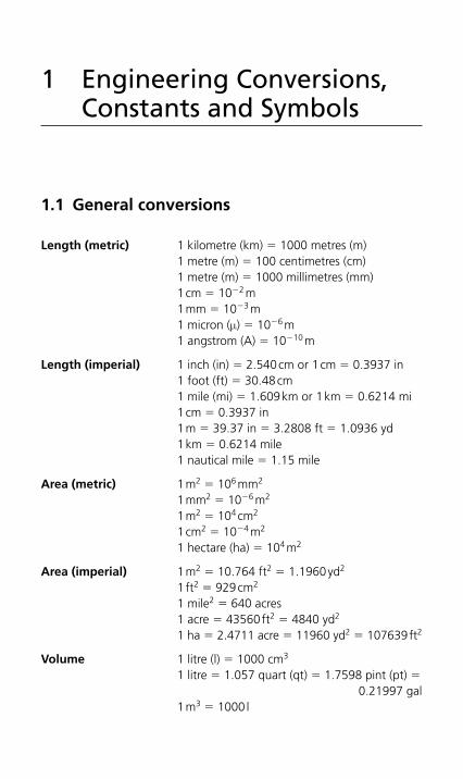
1.1 General conversions
Length (metric) 1 kilometre (km) � 1000 metres (m) 1 metre (m) � 100 centimetres (cm)
1 metre (m) � 1000 millimetres (mm) 1 cm � 10 � 2 m 1 mm � 10 � 3 m 1 micron ( μ ) � 10 � 6 m 1 angstrom (A) � 10 � 10 m
Length (imperial) 1 inch (in) � 2.540 cm or 1 cm � 0.3937 in 1 foot (ft) � 30.48 cm 1 mile (mi) � 1.609 km or 1 km � 0.6214 mi 1 cm � 0.3937 in 1 m � 39.37 in � 3.2808 ft � 1.0936 yd 1 km � 0.6214 mile 1 nautical mile � 1.15 mile
Area (metric) 1 m 2 � 10 6 mm 2 1 mm 2 � 10 � 6 m 2 1 m 2 � 10 4 cm 2 1 cm2 � 10 � 4 m 2 1 hectare (ha) � 10 4 m 2
Area (imperial) 1 m 2 � 10.764 ft 2 � 1.1960 yd 2 1 ft 2 � 929 cm 2 1 mile 2 � 640 acres 1 acre � 43560 ft 2 � 4840 yd 2 1 ha � 2.4711 acre � 11960 yd 2 � 107639 ft 2
Volume 1 litre (l) � 1000 cm 3 1 litre � 1.057 quart (qt) � 1.7598 pint (pt) �
0.21997 gal 1 m 3 � 1000 l
2 Engineering Mathematics Pocket Book
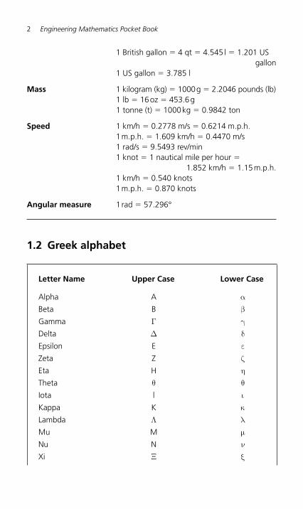
1 British gallon � 4 qt � 4.545 l � 1.201 US gallon
1 US gallon � 3.785 l
Mass 1 kilogram (kg) � 1000 g � 2.2046 pounds (lb) 1 lb � 16 oz � 453.6 g 1 tonne (t) � 1000 kg � 0.9842 ton
Speed 1 km/h � 0.2778 m/s � 0.6214 m.p.h. 1 m.p.h. � 1.609 km/h � 0.4470 m/s 1 rad/s � 9.5493 rev/min 1 knot � 1 nautical mile per hour �
1.852 km/h � 1.15 m.p.h. 1 km/h � 0.540 knots 1 m.p.h. � 0.870 knots
Angular measure 1 rad � 57.296 °
1.2 Greek alphabet
Letter Name Upper Case Lower Case
Alpha A α
Beta B β
Gamma Γ γ
Delta Δ δ
Epsilon E ε
Zeta Z ζ
Eta H η
Theta θ θ
Iota l ι
Kappa K κ
Lambda Λ λ
Mu M μ
Nu N ν
Xi Ξ ξ
Engineering Conversions, Constants and Symbols 3
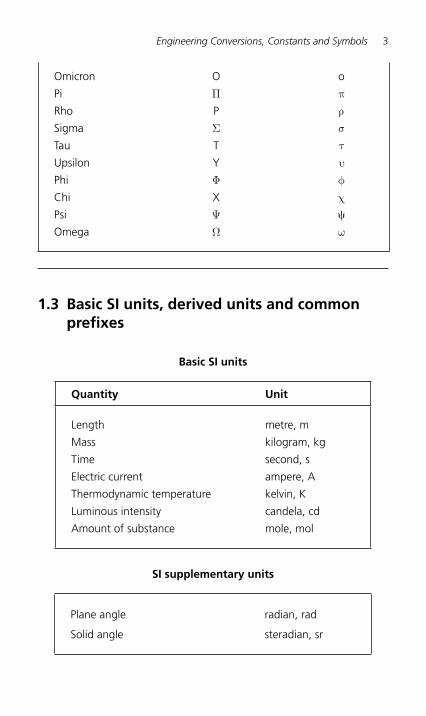
Omicron O o
Pi Π π
Rho P ρ
Sigma Σ σ
Tau T τ
Upsilon Y υ
Phi Φ φ
Chi X χ
Psi Ψ �
Omega Ω ω
1.3 Basic SI units, derived units and common prefixes
Basic SI units
Quantity Unit
Length metre, m
Mass kilogram, kg
Time second, s
Electric current ampere, A
Thermodynamic temperature kelvin, K
Luminous intensity candela, cd
Amount of substance mole, mol
SI supplementary units
Plane angle radian, rad
Solid angle steradian, sr
4 Engineering Mathematics Pocket Book
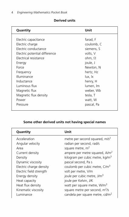
Derived units
Quantity Unit
Electric capacitance farad, F Electric charge coulomb, C Electric conductance siemens, S Electric potential difference volts, V Electrical resistance ohm, Ω Energy joule, J Force Newton, N Frequency hertz, Hz Illuminance lux, lx Inductance henry, H Luminous flux lumen, lm Magnetic flux weber, Wb Magnetic flux density tesla, T Power watt, W Pressure pascal, Pa
Some other derived units not having special names
Quantity Unit
Acceleration metre per second squared, m/s 2 Angular velocity radian per second, rad/s Area square metre, m 2 Current density ampere per metre squared, A/m 2 Density kilogram per cubic metre, kg/m 3 Dynamic viscosity pascal second, Pa s Electric charge density coulomb per cubic metre, C/m 3 Electric field strength volt per metre, V/m Energy density joule per cubic metre, J/m 3 Heat capacity joule per Kelvin, J/K Heat flux density watt per square metre, W/m 3 Kinematic viscosity square metre per second, m 2 /s Luminance candela per square metre, cd/m 2
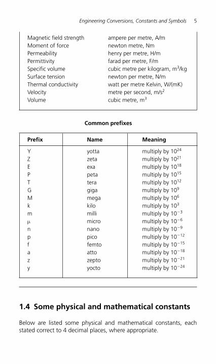
Engineering Conversions, Constants and Symbols 5
Magnetic field strength ampere per metre, A/m Moment of force newton metre, Nm Permeability henry per metre, H/m Permittivity farad per metre, F/m Specific volume cubic metre per kilogram, m3/kg Surface tension newton per metre, N/m Thermal conductivity watt per metre Kelvin, W/(mK) Velocity metre per second, m/s 2 Volume cubic metre, m 3
Common prefixes
Prefix Name Meaning
Y yotta multiply by 10 24 Z zeta multiply by 10 21 E exa multiply by 10 18 P peta multiply by 10 15 T tera multiply by 10 12 G giga multiply by 10 9 M mega multiply by 10 6 k kilo multiply by 10 3 m milli multiply by 10 � 3 μ micro multiply by 10 � 6 n nano multiply by 10 � 9 p pico multiply by 10 � 12 f femto multiply by 10 � 15 a atto multiply by 10 � 18 z zepto multiply by 10 � 21 y yocto multiply by 10 � 24
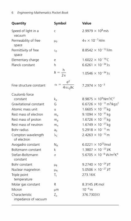
1.4 Some physical and mathematical constants
Below are listed some physical and mathematical constants, each stated correct to 4 decimal places, where appropriate.
6 Engineering Mathematics Pocket Book
Quantity Symbol Value
Speed of light in a vacuum
c 2.9979 � 10 8 m/s
Permeability of free space
μ 0 4π � 10 � 7 H/m
Permittivity of free space
ε 0 8.8542 � 10 � 12 F/m
Elementary charge e 1.6022 � 10 � 19 C
Planck constant h 6.6261 � 10 � 34 J s
� �
h2π 1.0546 � 10 � 34 J s
Fine structure constant α
πε�
ec
2
04 � 7.2974 � 10 � 3
Coulomb force constant ke 8.9875 � 10 9 Nm 2/C2
Gravitational constant G 6.6726 � 10 � 11 m3/kg s 2
Atomic mass unit u 1.6605 � 10 � 27 kg
Rest mass of electron m e 9.1094 � 10 � 31 kg
Rest mass of proton m p 1.6726 � 10 � 27 kg
Rest mass of neutron m n 1.6749 � 10 � 27 kg
Bohr radius a 0 5.2918 � 10 � 11 m
Compton wavelength of electron
λ C 2.4263 � 10 � 12 m
Avogadro constant N A 6.0221 � 10 23 /mol
Boltzmann constant k 1.3807 � 10 � 23 J/K
Stefan-Boltzmann constant
σ 5.6705 � 10 � 8 W /m 2 K 4
Bohr constant μ B 9.2740 � 10 � 24 J/T
Nuclear magnetron μ N 5.0506 � 10 � 27 J/T
Triple point temperature
T t 273.16 K
Molar gas constant R 8.3145 J/K mol
Micron μm 10 � 6 m
Characteristic impedance of vacuum
Z o 376.7303Ω
Engineering Conversions, Constants and Symbols 7
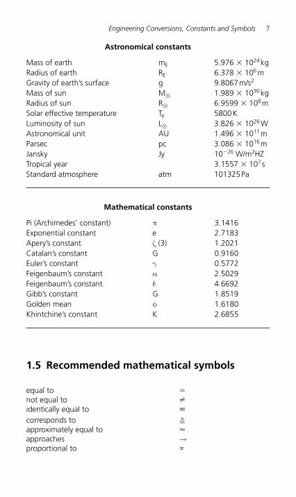
Astronomical constants
Mass of earth m E 5.976 � 10 24 kg Radius of earth R E 6.378 � 10 6 m Gravity of earth’s surface g 9.8067 m/s 2 Mass of sun M� 1.989 � 10 30 kg Radius of sun R� 6.9599 � 10 8 m Solar effective temperature Te 5800 K Luminosity of sun L� 3.826 � 10 26 W Astronomical uni t AU 1.496 � 10 11 m Parsec pc 3.086 � 10 16 m Jansky Jy 10 � 26 W/m 2 HZ Tropical year 3.1557 � 10 7 s Standard atmosphere atm 101325 Pa
Mathematical constants
Pi (Archimedes ’ constant) π 3.1416 Exponential constant e 2.7183 Apery’s constant ζ (3) 1.2021 Catalan’s constant G 0.9160 Euler’s constant γ 0.5772 Feigenbaum’s constant α 2.5029 Feigenbaum’s constant δ 4.6692 Gibb’s constant G 1.8519 Golden mean φ 1.6180 Khintchine’s constant K 2.6855
1.5 Recommended mathematical symbols
equal to � not equal to � identically equal to � corresponds to �
approximately equal to � approaches → proportional to �
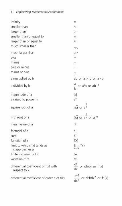
8 Engineering Mathematics Pocket Book
infinity �
smaller than
larger than
smaller than or equal to �
larger than or equal to �
much smaller than much larger than
plus �
minus �
plus or minus
minus or plus �
a multiplied by b ab or a � b or a � b
a divided by b
ab
or a/b or ab 1�
magnitude of a | a |
a raised to power n an
square root of a
a or a12
n’th root of a
a orn or a a1n 1/n
mean value of a a
factorial of a a!
sum Σ
function of x f(x)
limit to which f(x) tends as x approaches a
lim ( )x→a
f x
finite increment of x � x
variation of x δ x
differential coefficient of f(x) with respect to x
dfdx
or df/dy or f (x)�
differential coefficient of order n of f(x)
d fdx
n
n or d f/dx or f (x)n 2 n
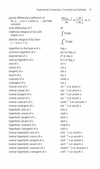
Engineering Conversions, Constants and Symbols 9
partial differential coefficient of f(x, y, …) w.r.t. x when y, … are held constant
∂∂
∂∂
⎛
⎝⎜⎜⎜
⎞
⎠⎟⎟⎟⎟
f(x,y,...)or or fxx
fx y
total differential of f df indefinite integral of f(x) with
respect to x f x dx( )∫
definite integral of f(x) from x � a to x � b
f x dx
a
b( )∫
logarithm to the base a of x loga X
common logarithm of x lg x or log10 x exponential of x ex or exp x natural logarithm of x ln x or loge x sine of x sin x cosine of x cos x tangent of x tan x secant of x sec x cosecant of x cosec x cotangent of x cot x inverse sine of x sin � 1 x or arcsin x inverse cosine of x cos � 1 x or arccos x inverse tangent of x tan � 1 x or arctan x inverse secant of x sec � 1 x or arcsec x inverse cosecant of x cosec � 1 x or arccosec x inverse cotangent of x cot � 1 x or arccot x hyperbolic sine of x sinh x hyperbolic cosine of x cosh x hyperbolic tangent of x tanh x hyperbolic secant of x sech x hyperbolic cosecant of x cosech x hyperbolic cotangent of x coth x inverse hyperbolic sine of x sinh � 1 x or arsinh x inverse hyperbolic cosine of x cosh � 1 x or arcosh x inverse hyperbolic tangent of x tanh � 1 x or artanh x inverse hyperbolic secant of x sech � 1 x or arsech x inverse hyperbolic cosecant of x cosech � 1 x or arcosech x inverse hyperbolic cotangent of x coth � 1 x or arcoth x
10 Engineering Mathematics Pocket Book
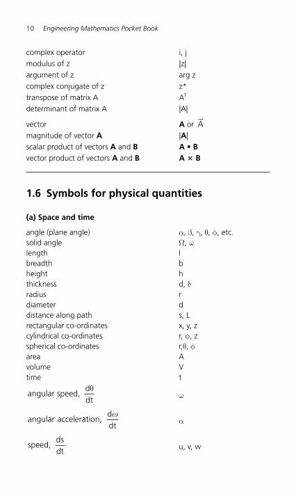
complex operator i, j modulus of z |z| argument of z arg z complex conjugate of z z* transpose of matrix A AT
determinant of matrix A |A|
vector A or A��
magnitude of vector A |A | scalar product of vectors A and B A • B vector product of vectors A and B A � B
1.6 Symbols for physical quantities
(a) Space and time angle (plane angle) α , β , γ , θ , φ , etc. solid angle Ω , ω length lbreadth bheight hthickness d, δ radius rdiameter d distance along path s, L rectangular co-ordinates x, y, z cylindrical co-ordinates r, φ , z spherical co-ordinates r, θ , φ area Avolume Vtime t
angular speed, dtdθ
ω
angulard
acceleration, dt�
α
speed,
dsdt
u, v, w
Engineering Conversions, Constants and Symbols 11
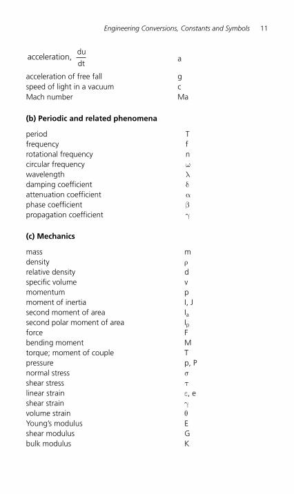
acceleration,
du
dt a
acceleration of free fall g speed of light in a vacuum c Mach number Ma
(b) Periodic and related phenomena
period Tfrequency f rotational frequency n circular frequency ω wavelength λ damping coefficient δ attenuation coefficient α phase coefficient β propagation coefficient γ
(c) Mechanics
mass mdensity ρ relative density d specific volume v momentum p moment of inertia I, J second moment of area I a second polar moment of area I p force F bending moment M torque; moment of couple Tpressure p, P normal stress σ shear stress τ linear strain ε , e shear strain γ volume strain θ Young’s modulus E shear modulus G bulk modulus K
12 Engineering Mathematics Pocket Book
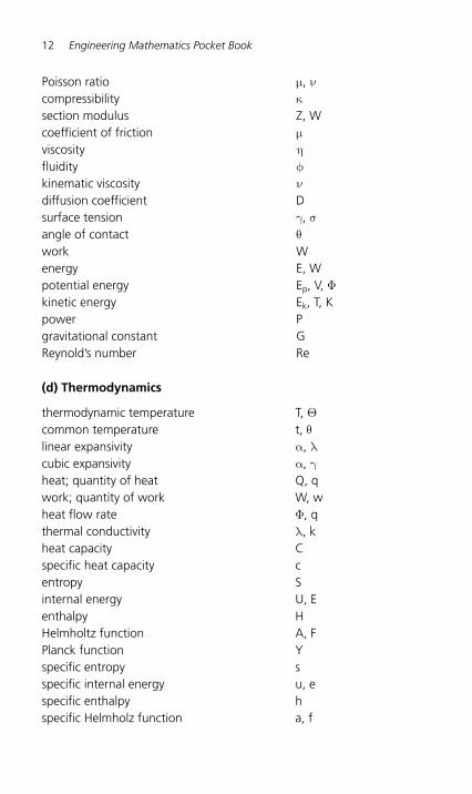
Poisson ratio μ , ν compressibility κ section modulus Z, W coefficient of friction μ viscosity η fluidity φ kinematic viscosity ν diffusion coefficient D surface tension γ , σ angle of contact θ work Wenergy E, W potential energy E p , V, Φ kinetic energy E k , T, K power P gravitational constant G Reynold’s number Re
(d) Thermodynamics
thermodynamic temperature T, Θ common temperature t, θ linear expansivity α , λ cubic expansivity α , γ heat; quantity of heat Q, q work; quantity of work W, w heat flow rate Φ , q thermal conductivity λ , k heat capacity C specific heat capacity c entropy S internal energy U, E enthalpy H Helmholtz function A, F Planck function Y specific entropy s specific internal energy u, e specific enthalpy h specific Helmholz function a, f
Engineering Conversions, Constants and Symbols 13
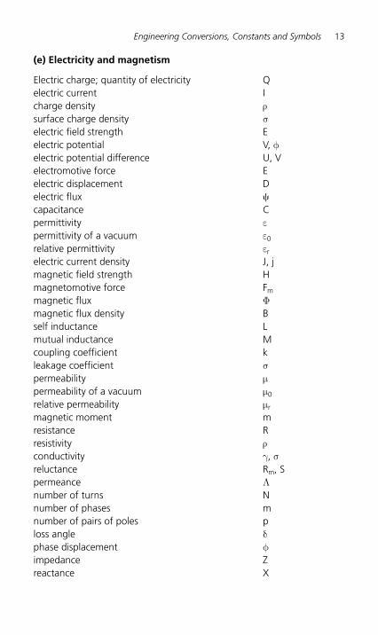
(e) Electricity and magnetism
Electric charge; quantity of electricity Q electric current I charge density ρ surface charge density σ electric field strength E electric potential V, φ electric potential difference U, V electromotive force E electric displacement D electric flux � capacitance Cpermittivity ε permittivity of a vacuum ε 0 relative permittivity ε r electric current density J, j magnetic field strength H magnetomotive force F m magnetic flux Φ magnetic flux density B self inductance L mutual inductance M coupling coefficient k leakage coefficient σ permeability μ permeability of a vacuum μ 0 relative permeability μ r magnetic moment m resistance Rresistivity ρ conductivity γ , σ reluctance Rm , S permeance Λ number of turns N number of phases m number of pairs of poles p loss angle δ phase displacement φ impedance Zreactance X
14 Engineering Mathematics Pocket Book
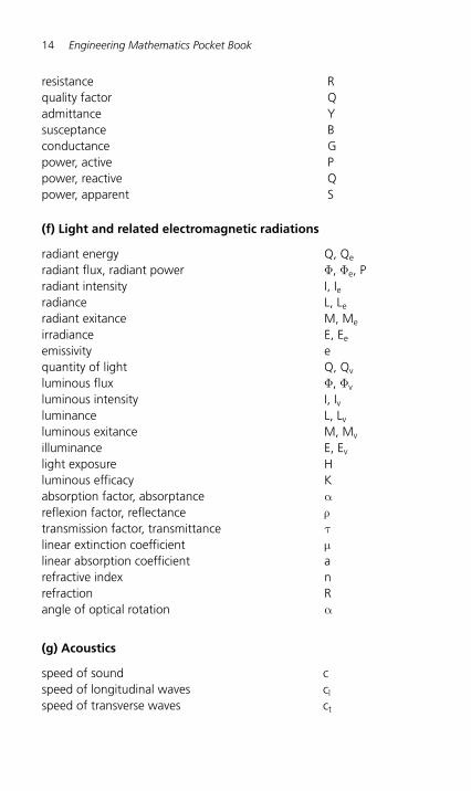
resistance R quality factor Q admittance Ysusceptance Bconductance G power, active P power, reactive Q power, apparent S
(f) Light and related electromagnetic radiations
radiant energy Q, Q e radiant flux, radiant power Φ , Φ e , P radiant intensity I, I e radiance L, L e radiant exitance M, M e irradiance E, E e emissivity e quantity of light Q, Q v luminous flux Φ , Φ v luminous intensity I, I v luminance L, L v luminous exitance M, M v illuminance E, E v light exposure H luminous efficacy K absorption factor, absorptance α reflexion factor, reflectance ρ transmission factor, transmittance τ linear extinction coefficient μ linear absorption coefficient a refractive index n refraction R angle of optical rotation α
(g) Acoustics
speed of sound c speed of longitudinal waves c l speed of transverse waves c t
Engineering Conversions, Constants and Symbols 15
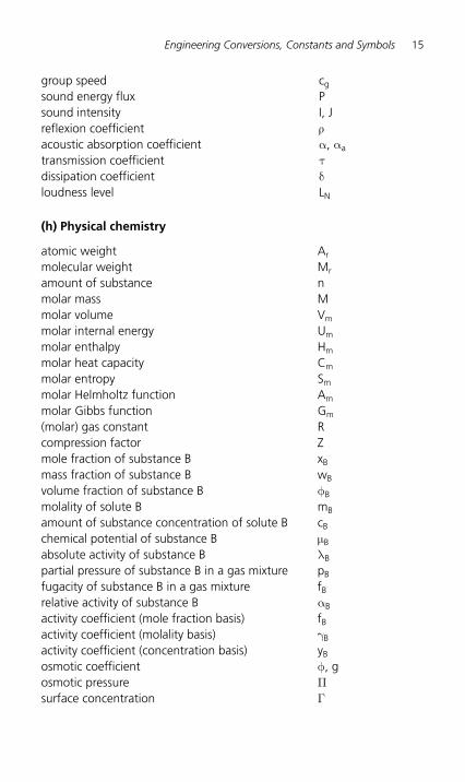
group speed c g sound energy flux P sound intensity I, J reflexion coefficient ρ acoustic absorption coefficient α , α a transmission coefficient τ dissipation coefficient δ loudness level L N
(h) Physical chemistry
atomic weight A r molecular weight M r amount of substance n molar mass M molar volume V m molar internal energy U m molar enthalpy H m molar heat capacity C m molar entropy S m molar Helmholtz function A m molar Gibbs function G m (molar) gas constant R compression factor Z mole fraction of substance B x B mass fraction of substance B w B volume fraction of substance B φ B molality of solute B m B amount of substance concentration of solute B c B chemical potential of substance B μ B absolute activity of substance B λ B partial pressure of substance B in a gas mixture p B fugacity of substance B in a gas mixture f B relative activity of substance B α B activity coefficient (mole fraction basis) f B activity coefficient (molality basis) γ B activity coefficient (concentration basis) y B osmotic coefficient φ , g osmotic pressure Π surface concentration Γ
16 Engineering Mathematics Pocket Book
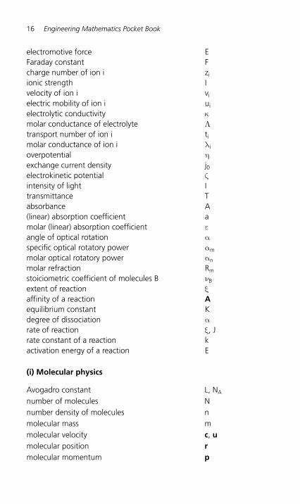
electromotive force E Faraday constant F charge number of ion i z i ionic strength I velocity of ion i v i electric mobility of ion i u i electrolytic conductivity κ molar conductance of electrolyte Λ transport number of ion i t i molar conductance of ion i λ i overpotential η exchange current density j 0 electrokinetic potential ζ intensity of light I transmittance Tabsorbance A (linear) absorption coefficient a molar (linear) absorption coefficient ε angle of optical rotation α specific optical rotatory power α m molar optical rotatory power α n molar refraction R m stoiciometric coefficient of molecules B ν B extent of reaction ξ affinity of a reaction A equilibrium constant K degree of dissociation α rate of reaction ξ , J rate constant of a reaction k activation energy of a reaction E
(i) Molecular physics
Avogadro constant L, N A number of molecules N number density of molecules n molecular mass m molecular velocity c, u molecular position r molecular momentum p
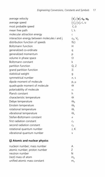
Engineering Conversions, Constants and Symbols 17
average velocity c u c u0 0, , , average speed c , , ,u c u most probable speed ˆ , ˆc u mean free path l, λ molecular attraction energy ε interaction energy between molecules i and j φ ij , V ij distribution function of speeds f(c) Boltzmann function H generalized co-ordinate q generalized momentum p volume in phase space Ω Boltzmann constant k partition function Q, Z grand partition function Ξ statistical weight g symmetrical number σ , s dipole moment of molecule p, μ quadrupole moment of molecule Θ polarizability of molecule α Planck constant h characteristic temperature Θ Debye temperature Θ D Einstein temperature Θ E rotational temperature Θ r vibrational temperature Θ v Stefan-Boltzmann constant σ first radiation constant c 1 second radiation constant c 2 rotational quantum number J, K vibrational quantum number v
(j) Atomic and nuclear physics
nucleon number; mass number A atomic number; proton number Z neutron number N (rest) mass of atom m a unified atomic mass constant m u
18 Engineering Mathematics Pocket Book
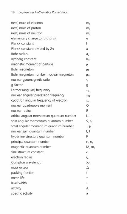
(rest) mass of electron m e
(rest) mass of proton m p
(rest) mass of neutron m n
elementary charge (of protons) e
Planck constant h
Planck constant divided by 2 π � Bohr radius a 0
Rydberg constant R �
magnetic moment of particle μ
Bohr magneton μ B
Bohr magneton number, nuclear magneton μ N
nuclear gyromagnetic ratio γ
g-factor g
Larmor (angular) frequency ω L
nuclear angular precession frequency ω N
cyclotron angular frequency of electron ω c
nuclear quadrupole moment Q
nuclear radius R
orbital angular momentum quantum number L, l 1
spin angular momentum quantum number S, s 1
total angular momentum quantum number J, j 1
nuclear spin quantum number I, J
hyperfine structure quantum number F
principal quantum number n, n 1
magnetic quantum number M, m 1
fine structure constant α
electron radius re
Compton wavelength λ C
mass excess Δ
packing fraction f
mean life τ
level width Γ
activity A
specific activity a
Engineering Conversions, Constants and Symbols 19
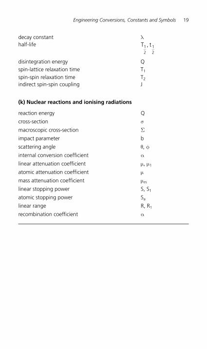
decay constant λ half-life T1
212
, t
disintegration energy Q spin-lattice relaxation time T 1 spin-spin relaxation time T 2 indirect spin-spin coupling J
(k) Nuclear reactions and ionising radiations
reaction energy Q
cross-section σ
macroscopic cross-section Σ
impact parameter b
scattering angle θ , φ
internal conversion coefficient α
linear attenuation coefficient μ , μ 1
atomic attenuation coefficient μ
mass attenuation coefficient μ m
linear stopping power S, S 1
atomic stopping power S a
linear range R, R 1
recombination coefficient α
2 Some Algebra Topics
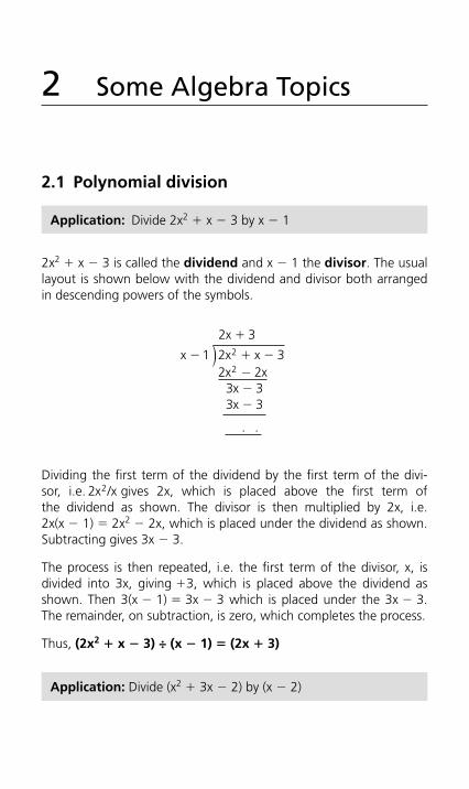
2.1 Polynomial division
Application: Divide 2x 2 � x � 3 by x � 1
2x 2 � x � 3 is called the dividend and x � 1 the divisor. The usual layout is shown below with the dividend and divisor both arranged in descending powers of the symbols.
)2 3
1 2 32 2
3 33 3
2
2
x
x
�
� � �
��
x xx x
xx
−
. .
Dividing the first term of the dividend by the first term of the divi-sor, i.e. 2 2x x/ gives 2x, which is placed above the first term of the dividend as shown. The divisor is then multiplied by 2x, i.e. 2x(x � 1) � 2x 2 � 2x, which is placed under the dividend as shown. Subtracting gives 3x � 3.
The process is then repeated, i.e. the first term of the divisor, x, is divided into 3x, giving � 3, which is placed above the dividend as shown. Then 3(x � 1) � 3x � 3 which is placed under the 3x � 3.The remainder, on subtraction, is zero, which completes the process.
Thus, (2x2 � x � 3) ÷ (x � 1) � (2x � 3)
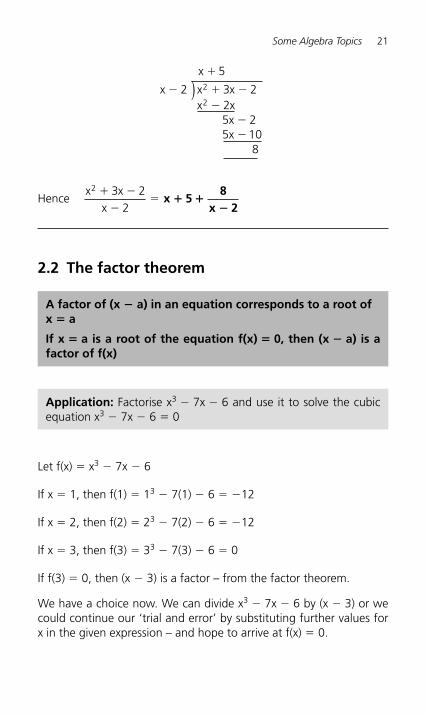
Application: Divide (x 2 � 3x � 2) by (x � 2)
Some Algebra Topics 21
)x
x
xx
�
� � �
���
5
2 3 225 25 10
8
2
2x xx x
Hencex
x
2 � �
��
3 22
xx 5
8x 2
� ��
2.2 The factor theorem
A factor of (x � a) in an equation corresponds to a root of x � a
If x � a is a root of the equation f(x) � 0, then (x � a) is a factor of f(x)
Application: Factorise x 3 � 7x � 6 and use it to solve the cubic equation x 3 � 7x � 6 � 0
Let f(x) � x 3 � 7x � 6
If x � 1, then f(1) � 1 3 � 7(1) � 6 � � 12
If x � 2, then f(2) � 2 3 � 7(2) � 6 � � 12
If x � 3, then f(3) � 3 3 � 7(3) � 6 � 0
If f(3) � 0, then (x � 3) is a factor – from the factor theorem.
We have a choice now. We can divide x 3 � 7x � 6 by (x � 3) or we could continue our ‘trial and error ’ by substituting further values for x in the given expression – and hope to arrive at f(x) � 0.
22 Engineering Mathematics Pocket Book
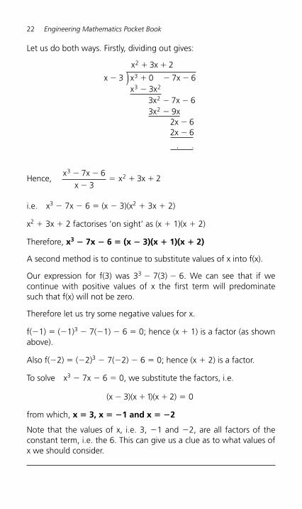
Let us do both ways. Firstly, dividing out gives:
)x
x
2 � �
� � � �
�
� �
���
3 2
3 0 7 633 7 63 9
2 62 6
3
3 2
2
2
x
x xx x
x xx x
xx
. .
Hence,x x
x
3 7 63
3 2� �
�� � �x x2
i.e. x 3 � 7x � 6 � (x � 3)(x 2 � 3x � 2)
x 2 � 3x � 2 factorises ‘ on sight ’ as (x � 1)(x � 2)
Therefore, x3 � 7x � 6 � (x � 3)(x � 1)(x � 2)
A second method is to continue to substitute values of x into f(x).
Our expression for f(3) was 3 3 � 7(3) � 6. We can see that if we continue with positive values of x the first term will predominate such that f(x) will not be zero.
Therefore let us try some negative values for x.
f( � 1) � ( � 1) 3 � 7(� 1) � 6 � 0; hence (x � 1) is a factor (as shown above).
Also f( � 2) � ( � 2) 3 � 7( � 2) � 6 � 0; hence (x � 2) is a factor.
To solve x 3 � 7x � 6 � 0, we substitute the factors, i.e.
(x )(x )(x )� � � �3 1 2 0
from which, x � 3, x � � 1 and x � �2
Note that the values of x, i.e. 3, �1 and �2, are all factors of the constant term, i.e. the 6. This can give us a clue as to what values of x we should consider.
Some Algebra Topics 23
2.3 The remainder theorem
If (ax 2 � bx � c) is divided by (x � p), the remainder will be ap2 � bp � c
If (ax 3 � bx 2 � cx � d) is divided by (x � p), the remainder will be ap 3 � bp 2 � cp � d
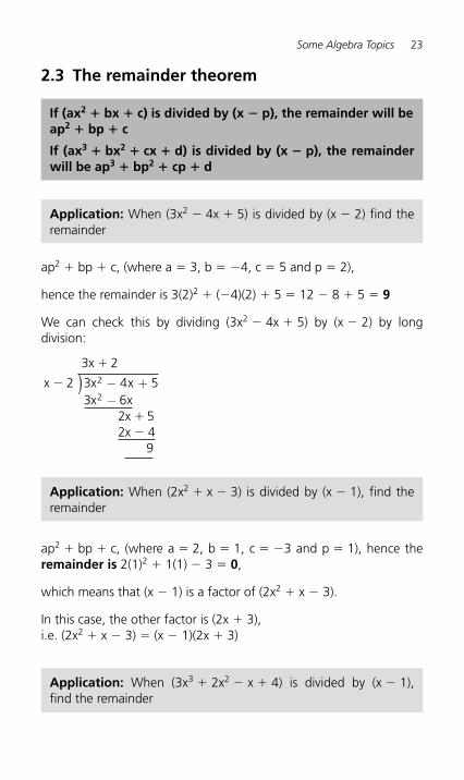
Application: When (3x 2 � 4x � 5) is divided by (x � 2) find the remainder
ap 2 � bp � c, (where a � 3, b � � 4, c � 5 and p � 2),
hence the remainder is 3(2) 2 � ( � 4)(2) � 5 � 12 � 8 � 5 � 9
We can check this by dividing (3x 2 � 4x � 5) by (x � 2) by long division:
)3 2
2 3 4 53 6
2 52 4
9
2
2
x
x
xx
�
�
��
x xx x
− +−
Application: When (2x 2 � x � 3) is divided by (x � 1), find the remainder
ap 2 � bp � c, (where a � 2, b � 1, c � � 3 and p � 1), hence the remainder is 2(1) 2 � 1(1) � 3 � 0 ,
which means that (x � 1) is a factor of (2x 2 � x � 3).
In this case, the other factor is (2x � 3), i.e. (2x 2 � x � 3) � (x � 1)(2x � 3)
Application: When (3x 3 � 2x 2 � x � 4) is divided by (x � 1), find the remainder
24 Engineering Mathematics Pocket Book
The remainder is ap 3 � bp 2 � cp � d (where a � 3, b � 2, c � � 1,d � 4 and p � 1), i.e. the remainder is: 3(1)3 � 2(1) 2 � ( � 1)(1) � 4 � 3 � 2 � 1 � 4 � 8
2.4 Continued fractions
Any fraction may be expressed in the form shown below for the fraction 26 55/ :
2655
15526
1
23
26
1
21
263
1
21
823
1
21
8132
1
21
81
112
� �
�
�
�
�
��
�
��
�
��
�
The latter factor can be expressed as: 1
A �
�
�
�
αβ
γδ
B
C
D Comparisons show that A, B, C and D are 2, 8, 1 and 2 respectively.
A fraction written in the general form is called a continued frac-tion and the integers A, B, C and D are called the quotients of the continued fraction. The quotients may be used to obtain closer and closer approximations, called convergents .
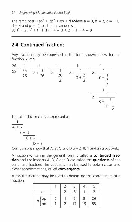
A tabular method may be used to determine the convergents of a fraction:
1 2 3 4 5
a 2 8 1 2
b
bpbq
⎧⎨⎪⎪⎩⎪⎪
01
12
817
919
2655
Some Algebra Topics 25
The quotients 2, 8, 1 and 2 are written in cells a2, a3, a4 and a5 with cell a1 being left empty.
The fraction 01 is always written in cell b1.
The reciprocal of the quotient in cell a2 is always written in cell b2, i.e. 1
2 in this case.
The fraction in cell b3 is given by ( )
( )
a b p b p
a b q b q,
3 2 1
3 2 1
� �
� �
i.e.( )( )8 1 08 2 1
817
� �
� ��
The fraction in cell b4 is given by (a b p) b p(a b q b q
,4 3 24 3 2
� �
� �)
i.e.( )
( )1 8 1
1 17 29
19� �
� �� , and so on.
Hence the convergents of2655
are 12
,8
17 ,
919
and2655
, each value
approximating closer and closer to 2655
.
These approximations to fractions are used to obtain practical ratios for gearwheels or for a dividing head (used to give a required angular displacement).
2.5 Solution of quadratic equations by formula
If ax 2 � bx � c � 0 then xb b 4ac
2a
2�
� � �
Comparing 3x 2 � 11x � 4 � 0 with ax 2 � bx � c � 0 gives a � 3, b � � 11 and c � � 4
Application: Solve 3x 2 � 11x � 4 � 0 by using the quadratic formula
26 Engineering Mathematics Pocket Book
Hence x,( ) ( ) ( )( )
( )�
� � � � ��
� �
� �
11 11 4 3 42 3
11 121 486
11 1696
11
2
136
11 136
11 136
�� �
or
Hence,
1or x 4
3� �
��
246
26
�
Application: Solve 4x 2 � 7x � 2 � 0 giving the roots correct to 2 decimal places
Comparing 4x 2 � 7x � 2 � 0 with ax 2 � bx � c gives a � 4, b � 7 and c � 2
Hence, x
or
�� �
��
��
�� � �
7 7 4 4 22 4
7 178
7 4 1238
7 4 1238
2 ( )( )( )
. . 77 4 1238
� .
Hence, x � � 0.36 or � 1.39, correct to 2 decimal places.
When height s � 16 m, 16 3012
9 81� �t t2( . )
i.e. 4.905t 2 � 30t � 16 � 0
Application: The height s metres of a mass projected vertically upwards at time t seconds is s ut gt� � 1
22 . Determine how long
the mass will take after being projected to reach a height of 16 m (a) on the ascent and (b) on the descent, when u � 30 m/s and g � 9.81 m/s 2
Some Algebra Topics 27
Using the quadratic formula:
t �� � � �
�
�
( ) ( ) ( . )( )( . )
..
.
30 30 4 4 905 162 4 905
30 586 19 81
30 24 21
2
99 815 53 0 59
.. .� or
Hence the mass will reach a height of 16 m after 0.59 s on the ascent and after 5.53 s on the descent.
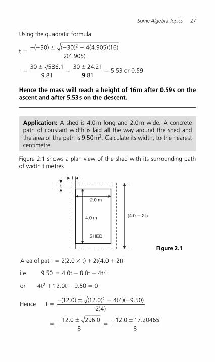
Application: A shed is 4.0 m long and 2.0 m wide. A concrete path of constant width is laid all the way around the shed and the area of the path is 9.50 m 2. Calculate its width, to the nearest centimetre
Figure 2.1 shows a plan view of the shed with its surrounding path of width t metres
2.0 m
4.0 m (4.0 � 2t)
SHED
t
t
Figure 2.1
Area of path t) t( t)� � � �2 2 0 2 4 0 2( . .
i.e. t t t9 50 4 0 8 0 4 2. . .� � �
or t t24 12 0 9 50 0� � �. .
Hence t �� � �
��
��
( . ) ( . ) ( )( . )( )
. . .
12 0 12 0 4 4 9 502 4
12 0 296 08
12 0
2
117 204658
.
28 Engineering Mathematics Pocket Book
Hence, t � 0.6506 m or � 3.65058 m
Neglecting the negative result which is meaningless, the width of the path, t � 0.651 m or 65 cm , correct to the nearest centimetre.
2.6 Logarithms
Definition of a logarithm: If y a then x log y
Laws of logar
xa� �
iithms: log (A B) log A log B
logAB
log A log B
lg
� � �
� �⎛⎝⎜⎜⎜
⎞⎠⎟⎟⎟⎟
A n log An �
(a) Let x � log 3 9 then 3 x � 9 from the definition of a logarithm,
i.e. 3 x � 3 2 , from which x � 2
Hence, log3 9 � 2
(b) Let x � log 16 8 then 16 x � 8, from the definition of a logarithm,
i.e. (2 4 ) x � 2 3 , i.e. 2 4x � 2 3 from the laws of indices, from
which, 4x � 3 and x �34
Hence, log 8
3416 �
Application: Evaluate (a) log 3 9 (b) log 16 8
Application: Evaluate (a) lg 0.001 (b) ln e (c) log3181
(a) Let x � lg 0.001 � log 10 0.001 then 10 x � 0.001, i.e. 10 x � 10 � 3 , from which x � � 3
Hence, lg 0.001 � � 3 (which may be checked by a calculator)
(b) Let x � ln e � log e e then e x � e, i.e. e x � e 1 from which x � 1.
Hence, ln e � 1 (which may be checked by a calculator)
Some Algebra Topics 29
(c) Let x � log3181
then 3181
13
34
4x � � � �
, from which x � � 4
Hence, log
181
43 � �
Application: Solve the equations: (a) lg x � 3 (b) log 5 x � � 2
(a) If lg x � 3 then log 10 x � 3 and x � 10 3 , i.e. x � 1000
(b) If log 5 x � � 2 then x � � ��515
22
125
Application: Solve 3 x � 27
Logarithms to a base of 10 are taken of both sides, i.e.
log log10 103 27x �
and log log10 103 27� by the third law of logarithms
Rearranging gives: x 3� � �
loglog
..
10
10
273
1 431360 4771
……
which may be
readily checked.
Application: Solve the equation 2 31 2 5x x� �� correct to 2 deci-mal places
Taking logarithms to base 10 of both sides gives:
log10 2 x � 1 � log 10 3 2x � 5
i.e. (x � 1)log 10 2 � (2x � 5)log 10 3
x log 10 2 � log 10 2 � 2x log 10 3 � 5 log 10 3
x(0.3010) � (0.3010) � 2x(0.4771) � 5(0.4771)
i.e. 0.3010x � 0.3010 � 0.9542x � 2.3855
Hence 2.3855 � 0.3010 � 0.9542x � 0.3010x
2.6865 � 0.6532x
from which, correct to 2 decimal placex 4.11� �
2 68650 6532..
, ss.
30 Engineering Mathematics Pocket Book
Application: Solve the equation x 3.2 � 41.15, correct to 4 sig-nificant figures
Taking logarithms to base 10 of both sides gives:
log 10 x 3.2 � log 10 41.15
3.2 log 10 x � log 10 41.15
Hence, xlog
log ..
.1010 41 153 2
0 50449� �
Thus, x � antilog 0.50449 � 10 0.50449 � 3.195 correct to 4 significant figures.
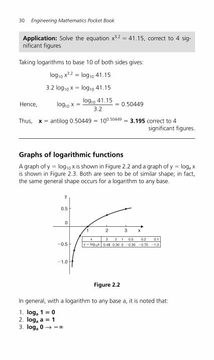
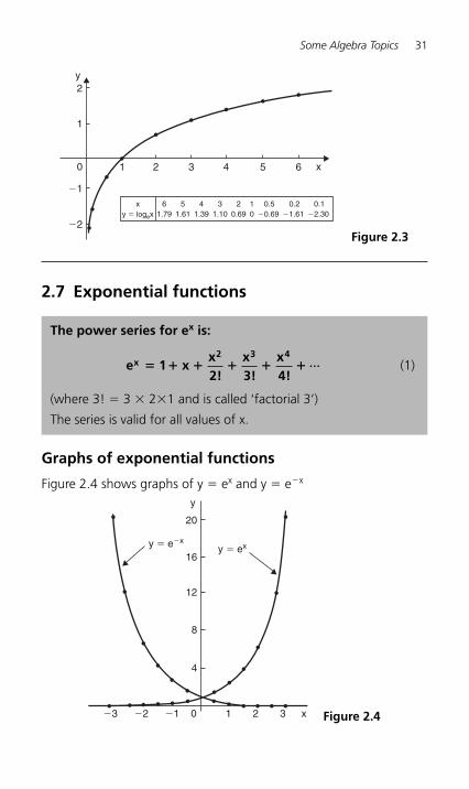
Graphs of logarithmic functions
A graph of y � log10 x is shown in Figure 2.2 and a graph of y � loge x is shown in Figure 2.3 . Both are seen to be of similar shape; in fact, the same general shape occurs for a logarithm to any base.
0.5
0
2 31
�0.5
�1.0
3
0.48
2
0.30
1
0
0.5
�0.30
0.2
�0.70
0.1
�1.0y � log10x
x
y
x
Figure 2.2
In general, with a logarithm to any base a, it is noted that:
1. loga 1 � 0 2. loga a � 1 3. loga 0 → � �
Some Algebra Topics 31
2.7 Exponential functions
2y
1
0 1 2 3 4 5 6
61.79
51.61
41.39
31.10
20.69
10
0.5�0.69
0.2�1.61
0.1�2.30
�1
�2y � logex
x
x
Figure 2.3
The power series for e x is:
e 1 xx2!
x3!
x4!
x2 3 4
� � � � � � ... (1)
(where 3! � 3 � 2 � 1 and is called ‘ factorial 3 ’ )
The series is valid for all values of x.
Graphs of exponential functions
Figure 2.4 shows graphs of y � e x and y � e � x
20
y
16y � e�x
y � ex
12
8
4
0�1 21 3 x�2�3 Figure 2.4
32 Engineering Mathematics Pocket Book
250
200
150
Vol
tage
v (v
olts
)
10080
50
0 1 1.5 2
Time t (seconds)
33.4 4 5 6
v = 250e−t /3
Figure 2.5
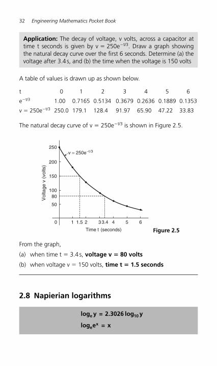
A table of values is drawn up as shown below.
t 0 1 2 3 4 5 6
e � t/3 1.00 0.7165 0.5134 0.3679 0.2636 0.1889 0.1353
v � 250e � t/3 250.0 179.1 128.4 91.97 65.90 47.22 33.83
The natural decay curve of v � 250e � t/3 is shown in Figure 2.5 .
Application: The decay of voltage, v volts, across a capacitor at time t seconds is given by v � 250e � t/3. Draw a graph showing the natural decay curve over the first 6 seconds. Determine (a) the voltage after 3.4 s, and (b) the time when the voltage is 150 volts
log y = 2.3026 log y
log e = x
e 10
ex
From the graph,
(a) when time t � 3.4 s, voltage v � 80 volts
(b) when voltage v � 150 volts, time t � 1.5 seconds
2.8 Napierian logarithms
Some Algebra Topics 33
Application: Solve e 3x � 8
Taking Napierian logarithms of both sides, gives
ln e
correct to
3x �
�
� �
ln
. . ln
ln
8
3 8
13
8
ie x
from which x 0.6931, 44 decimal places
Application: The work done in an isothermal expansion of a gas from pressure p 1 to p 2 is given by:
w wpp
1
2
� 0 ln⎛
⎝⎜⎜⎜⎜
⎞
⎠⎟⎟⎟⎟⎟
If the initial pressure p 1 � 7.0 kPa, calculate the final pressure p 2 if w � 3w0
If w � 3w 0 then 3 0 01w � w
pp2
ln⎛
⎝⎜⎜⎜⎜
⎞
⎠⎟⎟⎟⎟⎟
i.e. 3 � lnpp
1
2
⎛
⎝⎜⎜⎜⎜
⎞
⎠⎟⎟⎟⎟⎟
and e3 1
2 2
7000� �
pp p
from which,
,final pressure pe
e2 337000
7000� � �� 348.5 Pa
Laws of growth and decay
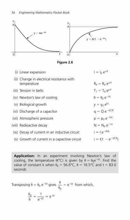
The laws of exponential growth and decay are of the form y � Ae � kx and y � A(1 � e � kx), where A and k are constants. When plotted, the form of each of these equations is as shown in Figure 2.6 . The laws occur frequently in engineering and science and examples of quantities related by a natural law include
34 Engineering Mathematics Pocket Book
(i) Linear expansion l � l 0 e α θ
(ii) Change in electrical resistance with temperature Rθ � R 0 e αθ
(iii) Tension in belts T1 � T 0 e μ θ
(iv) Newton’s law of cooling θ � θ 0 e � kt
(v) Biological growth y � y 0 e kt
(vi) Discharge of a capacitor q � Q e � t/CR
(vii) Atmospheric pressure p � p 0 e � h/c
(viii) Radioactive decay N � N 0 e � λ t
(ix) Decay of current in an inductive circuit i � I e � Rt/L
(x) Growth of current in a capacitive circuit i � I(1 � e � t/CR )
0
y � Ae�kx
y � A(1 � e�kx)
0
yA
yA
x x
Figure 2.6
Application: In an experiment involving Newton’s law of cooling, the temperature θ(°C) is given by θ � θ 0 e � kt. Find the value of constant k when θ 0 � 56.6°C, θ � 16.5°C and t � 83.0 seconds
Transposing θ � θ 0 e � kt gives θθ0
� �e kt from which,
θθ0 1
� ��e
ekt
kt
Some Algebra Topics 35
Taking Napierian logarithms of both sides gives: lnθθ0 � kt
fromwhicht
, ln.
ln.. .
( .k � � �1 1
83 056 616 5
183 0
1 230θθ
⎛⎝⎜⎜⎜
⎞⎠⎟⎟⎟⎟ 226486 ..)
� 1.485 10 2� �
Application: The current i amperes flowing in a capacitor at time t seconds is given by i � 8.0(1 � e � t/CR), where the circuit resist-ance R is 25 k Ω and capacitance C is 16 μF. Determine (a) the cur-rent i after 0.5 seconds and (b) the time, to the nearest ms, for the current to reach 6.0 A
(a) Current i e ) et/CR� � � �
�
� � � ��8 0 1 8 01 0 5 16 10 25 106 3. ( . [ ]. /( )( )
88 0 1
8 0 1 0 2865047 8 0 0 7134952
1 25. ( )
. ( . ..) . ( . ..)
.�
� � �
�
�e
5.71 ampeeres
(b) Transposing i � 8.0(1 � e � t/CR ) gives: i
e t/CR
801� � �
from which, ei it/CR� � � �
�1
8 08 0
8 0..
.
Taking the reciprocal of both sides gives: ei
t/CR ��
8 08 0
..
Taking Napierian logarithms of both sides gives:
tCR i
��
ln.
.8 0
8 0
⎛⎝⎜⎜⎜
⎞⎠⎟⎟⎟⎟
Hence t CRi
��
ln.
.8 0
8 0
⎛⎝⎜⎜⎜
⎞⎠⎟⎟⎟⎟
� � �
��( )( ) ln
.. .
16 10 25 108 0
8 0 6 06 3
⎛⎝⎜⎜⎜
⎞⎠⎟⎟⎟⎟ when i � 6.0
amperes,
36 Engineering Mathematics Pocket Book
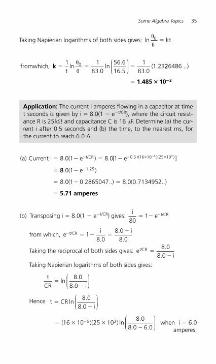
i.e. t � �
�
�
0 40 0 4 4 0
0 4 1 3862943
0 55
. . .
. ( . ..)
.
ln8.02.0
ln ⎛⎝⎜⎜⎜
⎞⎠⎟⎟⎟⎟
445 s
� 555 ms, to the nearest millisecond. A graph of current against time is shown in Figure 2.7 .
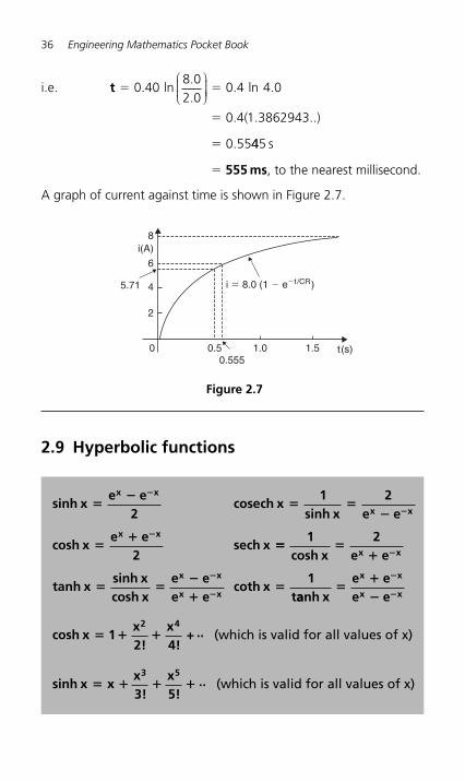
sinh xe e
2cosech x
1sinh x
2e e
cosh xe e
2sech x
x x
x x
x x
��
� ��
��
�
�
�
�� ��
� ��
��
�
�
�
1cosh x
2e e
tanh xsinh xcosh x
e ee e
coth x1
t
x x
x x
x x aanh xe ee e
x x
x x�
�
�
�
�
cosh x 1x2!
x4!
+ ..2 4
� � � (which is valid for all values of x)
sinh x xx3!
x5!
..3 5
� � � � (which is valid for all values of x)
2.9 Hyperbolic functions
8
6
5.71
0.555
4
2
0 0.5 1.0 1.5
i � 8.0 (1 � e�t /CR)
t(s)
i(A)
Figure 2.7
Some Algebra Topics 37
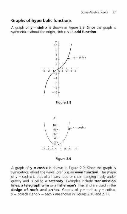
Graphs of hyperbolic functions
A graph of y � sinh x is shown in Figure 2.8 . Since the graph is symmetrical about the origin, sinh x is an odd function .
0 1 2 3�3 �2 �1�2
2
4
6
8
10
�4
�6
�8
�10
x
y � sinh x
y
Figure 2.8
10
8
6
4
2
0 1 2 3 x
y
y � cosh x
�1�2�3
Figure 2.9
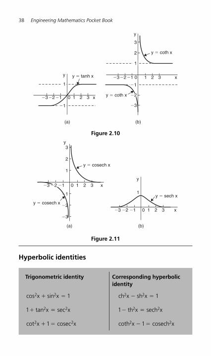
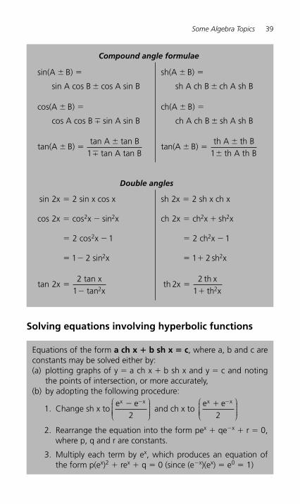
A graph of y � cosh x is shown in Figure 2.9 . Since the graph is symmetrical about the y-axis, cosh x is an even function. The shape of y � cosh x is that of a heavy rope or chain hanging freely under gravity and is called a catenary. Examples include transmissionlines, a telegraph wire or a fisherman’s line, and are used in the design of roofs and arches. Graphs of y � tanh x, y � coth x, y � cosech x and y � sech x are shown in Figures 2.10 and 2.11 .
38 Engineering Mathematics Pocket Book
Hyperbolic identities
Trigonometric identity Corresponding hyperbolic identity
cos x sin x2 2 1� � ch x sh x2 2 1� �
12 2� �tan x sec x 1 2 2� �th x sech x
cot x cosec x2 21� � coth x cosech x2 21� �
0 1 2 3 x�1�2�3
0 1 2 3 x
y
y�1�2�3
�3
2
3
y � tanh x
y � coth x
y � coth x
1
1
�1
�1
�2
(a) (b)
Figure 2.10
0 1 2 3 x
y
�1�3
�3
�2
�1
1
2
3
y � cosech x
y � cosech x
(a) (b)
0 1 2 3 x
y
�1�2�3
1y � sech x
�2
Figure 2.11
Some Algebra Topics 39
Compound angle formulae
sin(A B)
sin A cos B cos A sin B
�
sh(A B)
sh A ch B ch A sh B
�
cos(A B)
cos A cos B sin A sin B
�
�
ch(A B)
ch A ch B sh A sh B
�
tan(A B)
tan A tan Btan A tan B
�
�1 tan(A B)
th A th Bth A th B
�
1
Double angles
sin x sin x cos x2 2� sh x sh x ch x2 2�
cos x cos x sin x2 2 2� � ch x ch x sh x2 2 2� �
� �2 12 cos x � �2 12 ch x
� �1 2 2 sin x � �1 2 2sh x
tan x
tan xtan x
22
1 2�
� th x
th xth x
22
1 2�
�
Equations of the form a ch x � b sh x � c, where a, b and c are constants may be solved either by: (a) plotting graphs of y � a ch x � b sh x and y � c and noting
the points of intersection, or more accurately, (b) by adopting the following procedure:
1. Change sh x to e ex x� �
2
⎛
⎝⎜⎜⎜⎜
⎞
⎠⎟⎟⎟⎟ and ch x to
e ex x� �
2
⎛
⎝⎜⎜⎜⎜
⎞
⎠⎟⎟⎟⎟
2. Rearrange the equation into the form pe x � qe � x � r � 0, where p, q and r are constants.
3. Multiply each term by e x, which produces an equation of the form p(e x ) 2 � re x � q � 0 (since (e � x )(e x ) � e 0 � 1)
Solving equations involving hyperbolic functions
40 Engineering Mathematics Pocket Book
Following the above procedure:
1. sh x
e ex x�
��
�
23
⎛
⎝⎜⎜⎜⎜
⎞
⎠⎟⎟⎟⎟
2. e x � e � x � 6, i.e. e x � e � x � 6 � 0
3. (e x ) 2 � (e � x )(e x ) � 6e x � 0, i.e. (e x ) 2 � 6e x � 1 � 0
4. ex �
� � � � ��
�
( ) [( ) ( )( )]( )
.6 6 4 1 12 1
6 402
6 6 32462
2
Hence, e x � 6.1623 or � 0.1623
5. x � ln 6.1623 or x � ln(�0.1623) which has no solution since it is not possible in real terms to find the logarithm of a negative number.
Hence x � ln 6.1623 � 1.818 , correct to 4 significant figures.
4. Solve the quadratic equation p(e x ) 2 � re x � q � 0 for e x by factorising or by using the quadratic formula.
5. Given e x � a constant (obtained by solving the equa-tion in 4), take Napierian logarithms of both sides to give x � ln(constant)
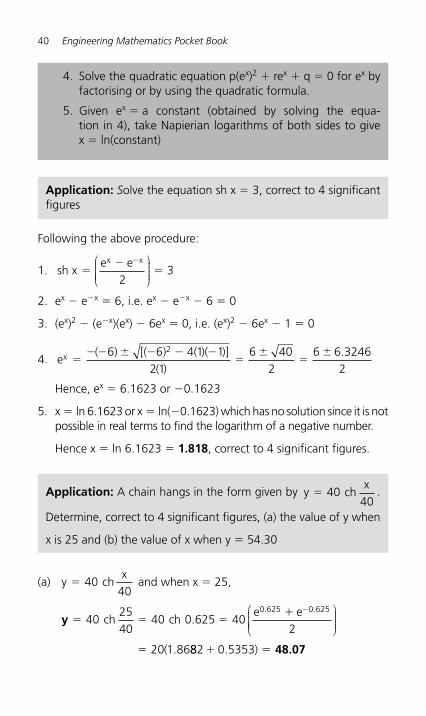
Application: Solve the equation sh x � 3, correct to 4 significant figures
Application: A chain hangs in the form given by y chx
� 4040
.
Determine, correct to 4 significant figures, (a) the value of y when
x is 25 and (b) the value of x when y � 54.30
(a) y chx
� 4040
and when x � 25,
y � � ��
�
�
402540
40 402
20 1 86
0 625 0 625ch ch 0.625
e e. .
( .
⎛
⎝⎜⎜⎜⎜
⎞
⎠⎟⎟⎟⎟
882 0 5353� �. ) 48.07
Some Algebra Topics 41
(b) When y chx
� �54 30 54 30 4040
. , . , from which
chx
40�
54 3040
1 3575.
.�
Following the above procedure:
1.
e ex/ x/40 40
21 3575
��
�
.
2. e x/40 � e � x/40 � 2.715 i.e. e x/40 � e � x/40 � 2.715 � 0
3. (e x/40 ) 2 � 1 � 2.715 e x/40 � 0 i.e. (e x/40 ) 2 � 2.715 e x/40 � 1 � 0
4. ex/4022 715 2 715 4 1 1
2 1
2 715 3 37122
2
�� � � �
�
�
( . ) [( . ) ( )( )]( )
. ( . ) .7715 1 83612
.
Hence e x/40 � 2.2756 or 0.43945
5.
xln 2.2756
40�
or
xln
400 43945� ( . )
Hence, x
400 8222� .
or
x40
0 8222� � .
Hence, x � 40(0.8222) or x � 40( � 0.8222)
i.e. x � � 32.89 , correct to 4 significant figures.
2.10 Partial fractions
Provided that the numerator f(x) is of less degree than the rel-evant denominator, the following identities are typical examples of the form of partial fraction used:
Linear factors
f(x)(x a)(x b)(x c)
A(x a)
B(x b)
C(x c)� � �
���
��
��
42 Engineering Mathematics Pocket Book
The denominator factorises as (x � 1)(x � 3) and the numerator is of less degree than the denominator.
Thus 11 32 32
�
� �
xx x
may be resolved into partial fractions.
Let 11 3
2 311 3
1 3 1 32
�
� ��
�
� � ��
�
xx x
xx x
Ax
Bx( )( ) ( ) ( )
� where A and
B are constants to be determined,
i.e.11 3
1 33 11 3
�
� �
� � �
� �
xx x
A x B xx x
by algebraic additi( )( )
( ) ( )( )( )
� oon
Since the denominators are the same on each side of the identity then the numerators are equal to each other.
Thus, 11 3 3 1� � � � �x A(x ) B(x ) To determine constants A and B, values of x are chosen to make the term in A or B equal to zero.
When x � 1, then 11 � 3(1) � A(1 � 3) � B(0)
i.e. 8 4� A i.e. A 2�
When x � � 3, then 11 � 3( � 3) � A(0) � B( � 3 � 1)
i.e. 20 4� � B
i.e. B 5� �
Repeated linear factors
f(x)(x a)
A(x a)
B(x a)
C(x a)3 2 3� �
��
��
≡
Quadratic factors
f(x)(ax bx c)(x d)
Ax B(ax bx c)
C(x d)2 2� � �
�
� ��
�≡
Application: Resolve 11 3
2 32
�
� �
xx x
into partial fractions
Some Algebra Topics 43
Thus
(x ) (x11 3x
x 2x 32
(x 1)5
(x 3)2
�
� � ��
��
��
�
��
21
53)
Check:
) )( ) ( )
( )( )(x (xx x
x xx
x x2
15
32 3 5 1
1 311 3
2 32��
��
� � �
� ��
�
� �
⎡
⎣⎣⎢⎢
⎤
⎦⎥⎥
Application: Express x x xx x
3 2� � �
� �
2 4 422
in partial fractions
The numerator is of higher degree than the denominator. Thus divid-ing out gives:
)x
x x x xx x x
x xx x
x
�
� � � � �
� �
� � �
� � �
�
3
2 2 4 42
3 2 43 3 6
10
2 3 2
3 2
2
2
x
Thus x x x
x xx
xx x
xx
(x x
3 2
2 2
2 4 42
310
2
310
2
� � �
� �� �
�
� �
� ��
�
�
�)( �� 1)
Let
x(x x
A(x
Bx
A(x B x(x x
�
� � ��
��
� � �
� �
102 1 2 1
1 22 1)( ) ) ( )) ( )
)( )�
Equating the numerators gives: x � 10 � A(x � 1) � B(x � 2)
Let x � � 2, then � � �12 3A i.e. A 4�
Let x � 1, then � �9 3B
i.e. B 3� �
Hence
xx x x x
�
� ��
��
�
102 1
42
31( )( ) ( ) ( )
44 Engineering Mathematics Pocket Book
Thus
x 2x 4x 4x x 2
x 34
(x 2)3
(x 1)
3 2
2
� � �
� �� � �
��
�
Application: Express 5 2 19
3 1
2
2
x x(x (x
� �
� �) ) as the sum of three partial
fractions
The denominator is a combination of a linear factor and a repeated linear factor.
Let
5 2 193 1 3 1 1
1 3
2
2 2
2
x xx x
A(x
B(x
C(x
A(x B(x
� �
� ��
��
��
�
�� � �
( )( ) ) ) )
) )(xx C(x(x (x
by algebraic� � �
� �
1 33 1 2
) )) ) addition
Equating the numerators gives:
5 2 19 1 3 1 32 2x x A(x (x x C(x� � � � � � � �� ) )( ) )B (1)
Let x � � 3, then 5( �3)2 � 2(�3) � 19 � A(�4)2 � B(0)(�4) � C(0)
i.e. 32 16� A
i.e. A 2�
Let x � 1, then 5(1) 2 � 2(1) � 19 � A(0) 2 � B(4)(0) � C(4)
i.e. � �16 4C
i.e. C 4� �
Without expanding the RHS of equation (1) it can be seen that equating the coefficients of x 2 gives:
5 � A � B, and since A � 2, B � 3
Hence
5x 2x 19(x 3)(x 1)
2(x 2)
3(x 1)
4(x 1)
2
2 2
� �
� � ��
��
�≡
Some Algebra Topics 45
Application: Resolve 3 6 4 23
2 3
2 2
� � �
�
x x xx (x )
into partial fractions
Terms such as x 2 may be treated as (x � 0) 2, i.e. they are repeated linear factors.
(x 2 � 3) is a quadratic factor which does not factorise without con-taining surds and imaginary terms.
Let x x xx x
Ax
Bx
Cx Dx
Ax x B x
3 6 4 23 3
3 3
2 3
2 2 2 2
2 2
� � �
�� � �
�
�
�� � �
( ) ( )
( ) ( )) ( )( )
� �
�
Cx D xx x
2
2 2 3
Equating the numerators gives:
3 6 4 2 3 3
3 3
2 3 2 2 2
3 2 3
� � � � � � � � �
� � � � � �
x x Ax(x B(x (Cx D)x
Ax Ax Bx B Cx
x ) )
DDx2
Let x � 0, then 3 3� B i.e. B 1� Equating the coefficients of x 3 terms gives: � � �2 A C (1) Equating the coefficients of x 2 terms gives: 4 � �B D Since B � 1, D � 3
Equating the coefficients of x terms gives: 6 3� A i.e. A 2� From equation (1), since A � 2, C � � 4
Hence x x
xx
3 6x 4x 2xx (x 3)
2x
1x
3 4xx
2 3
2 2
2 2
� � �
�
� ��
�
� � �� �
�
�
2 1 4 332 2
33
3 Some Number Topics
3.1 Arithmetic progressions
If a � first term, d � common difference and n � number of terms, then the arithmetic progression is:
a, a d, a 2d, ....� � The n’th term is:
a (n 1)d� � The sum of n terms,
Sn2
[2a (n 1)d]n � � �
Application: Find the sum of the first 7 terms of the series 1, 4, 7, 10, 13, . . .
The sum of the first 7 terms is given by
S [ ( ) ( ) ] since a and d7
72
2 1 7 13 1 3� � � � �
� � � �72
2 1872
20[ ] [ ] 70
Application: Determine (a) the ninth, and (b) the sixteenth term of the series 2, 7, 12, 17, . . .
2, 7, 12, 17, ..... is an arithmetic progression with a common differ-ence, d, of 5
Some Number Topics 47
(a) The n’th term of an AP is given by a � (n � 1)d Since the first term a � 2, d � 5 and n � 9 then the 9th term is: 2 � (9 � 1)5 � 2 � (8)(5) � 2 � 40 � 42
(b) The 16th term is: 2 � (16 � 1)5 � 2 � (15)(5) � 2 � 75 � 77
Application: Find the sum of the first 12 terms of the series 5, 9, 13, 17, .....
5, 9, 13, 17, ..... is an AP where a � 5 and d � 4
The sum of n terms of an AP, S
n[ a (n )d]n � � �
22 1
Hence the sum of the first 12 terms, S [ ( ) ( ) ]12122
2 5 12 1 4� � �
�� � �
�
610 44 6 54[ ] ( )
324
3.2 Geometric progressions
If a � first term, r � common ratio and n � number of terms, then the geometric progression is:
a, ar, ar , ar , ....2 3
The n’th term is: arn 1�
The sum of n terms,
Sa(1 r )(1 r)
which is valid when r 1n
n�
�
�<
or
Sa(r 1)(r 1)
which is valid when r 1n
n�
�
�>
If � 1 < r < 1, Sa
(1 r)∞ ��
48 Engineering Mathematics Pocket Book
The sum of the first 8 terms is given by
S( )( )
since a and r8
812 12 1
1 2��
�� �
i.e. S8 ��
�1256 1
1( )
255
Application: Find the sum of the first 8 terms of the GP 1, 2, 4, 8, 16, ....
Application: Determine the tenth term of the series 3, 6, 12, 24, ....
3, 6, 12, 24, .... is a geometric progression with a common ratio r of 2.
The n’th term of a GP is ar n � 1 , where a is the first term.
Hence the 10th term is: (3)(2) 10 � 1 � (3)(2) 9 � 3(512) � 1536
The net gain forms a series: £400 � £400 � 0.9 � £400 � 0.92 � .....,
which is a GP with a � 400 and r � 0.9
The sum to infinity,
Sa
r� ��
��
� �( ) ( )1
4001 0 9.
£4000 total future profits
Application: A hire tool firm finds that their net return from hir-ing tools is decreasing by 10% per annum. Their net gain on a certain tool this year is £400. Find the possible total of all future profits from this tool (assuming the tool lasts for ever)
Application: A drilling machine is to have 6 speeds ranging from 50 rev/min to 750 rev/min. Determine their values, each cor-rect to the nearest whole number, if the speeds form a geometric progression
Some Number Topics 49
Let the GP of n terms be given by a, ar, ar 2 , .... ar n � 1
The first term a � 50 rev/min
The 6th term is given by ar 6 � 1 , which is 750 rev/min,
i.e. ar 5 � 750
from which r
a5 750 750
5015� � �
Thus the common ratio, r � �15 1 71885 .
The first term is a � 50 rev/min
the second term is ar � (50)(1.7188) � 85.94,
the third term is ar 2 � (50)(1.7188) 2 � 147.71,
the fourth term is ar 3 � (50)(1.7188) 3 � 253.89,
the fifth term is ar 4 � (50)(1.7188) 4 � 436.39,
the sixth term is ar 5 � (50)(1.7188) 5 � 750.06
Hence, correct to the nearest whole number, the 6 speeds of the drilling machine are:
50, 86, 148, 254, 436 and 750 rev/min
3.3 The binomial series
(a x) a na xn(n 1)
2!a x
n(n 1)(n 2)3!
a x ...
n n n 1 n 2 2
n 3 3
� � � ��
�� �
�
� �
� ... xn�
(1 x) 1 nxn(n 1)
2!x
n(n 1)(n 2)3!
x .......n 2 3� � � ��
�� �
�
which is valid for 1 x 1� < <
The r’th term of the expansion (a � x) n is:
n(n 1)(n 2) .... to (r 1) terms(r 1)!
a xn (r 1) r 1� � �
�� � �
50 Engineering Mathematics Pocket Book
From above, when a � 2 and n � 7:
( x) 2 7(2) x( )( )( )( )
( )( )( )( )( )( )( )
( )27 62 1
27 6 53 2 1
27 7 6 5 2 4� � � � �x xx
( )( )( )( )( )( )( )( )
( ) x( )( )( )( )( )( )( )
3
3 47 6 5 44 3 2 1
27 6 5 4 35 4
� �(( )( )( )
( ) x
( )( )( )( )( )( )( )( )( )( )( )( )
( )x
3 2 12
7 6 5 4 3 26 5 4 3 2 1
2
2 5
� 66 77 6 5 4 3 2 17 6 5 4 3 2 1
�( )( )( )( )( )( )( )( )( )( )( )( )( )( )
x
i.e.
(2 � x)7 � 128 � 448x � 672x2 � 560x3 � 280x4 � 84x5 � 14x6 � x7
Application: Using the binomial series, determine the expansion of (2 � x) 7
Application: Determine the fifth term (3 � x) 7 without fully expanding
The r’th term of the expansion (a � x)n is given by:
n(n )(n )... to (r ) terms(r )!
a xn (r ) r� � �
�� � �1 2 1
11 1
Substituting n � 7, a � 3 and r � 1 � 5 � 1 � 4 gives:
( )( )( )( )( )( )( )( )
( ) x7 6 5 44 3 2 1
3 7 4 4�
i.e. the fifth term of (3 � x)7 � 35(3) 3 x 4 � 945x4
Application: Expand 11 2 3( x)�
in ascending powers of x as far
as the term in x 3 , using the binomial series
Some Number Topics 51
Using the binomial expansion of (1 � x) n, where n � � 3 and x is replaced by 2x gives:
11 2
1 2
1 3 23 42
23 4 5
3
33
2
( x)( x)
( )( x)( )( )
!( x)
( )( )( )�
� �
� � � �� �
�� � �
�
!!( x) ..2 3 �
� 1 6x 24x 80x2 3� � � �
The expansion is valid provided x2 1
i.e. orx12
12
x12
< < <�
Application: Using the binomial theorem, expand 4 � x in ascending powers of x to four terms
4 4 14
4 14
2 14
� � � � � � �xx x x⎛
⎝⎜⎜⎜
⎞⎠⎟⎟⎟⎟
⎡
⎣⎢⎢
⎤
⎦⎥⎥
⎛⎝⎜⎜⎜
⎞⎠⎟⎟⎟⎟
⎛⎝⎜⎜⎜
⎞⎠⎟⎟⎟⎟⎟
1 2/
Using the expansion of (1 � x) n ,
2 14
2 112 4
1 2
1 2
�
� � ��
x
x ( / )(
/⎛⎝⎜⎜⎜
⎞⎠⎟⎟⎟⎟
⎛⎝⎜⎜⎜
⎞⎠⎟⎟⎟⎟⎛⎝⎜⎜⎜
⎞⎠⎟⎟⎟⎟
11 22 4
1 2 1 2 3 23 4
2 3/ )
!x ( / )( / )( / )
!x⎛
⎝⎜⎜⎜
⎞⎠⎟⎟⎟⎟
⎛⎝⎜⎜⎜
⎞⎠⎟⎟⎟⎟�
� �� ..
⎡⎡
⎣
⎢⎢⎢
⎤
⎦
⎥⎥⎥
⎛
⎝⎜⎜⎜⎜
⎞
⎠⎟⎟⎟⎟� � � � �
�
2 18 128 1024
2 3x x x ..
2x4
x64
x2 3� � �
5512.....�
This is valid when
x, i.e. or
41 x 4 4 x 4< < <�
52 Engineering Mathematics Pocket Book
( x) ( x)
x( x) ( )
1 3 1
12
1 3 1 12
3
3
13
12
� �
�
� � � �⎛⎝⎜⎜⎜
⎞⎠⎟⎟⎟⎟
⎛⎝⎜⎜⎜
⎞⎠⎟⎟⎟x
x⎟⎟
⎛⎝⎜⎜⎜
⎞⎠⎟⎟⎟⎟
⎡
⎣⎢⎢
⎤
⎦⎥⎥
⎛⎝⎜⎜⎜
⎞⎠⎟⎟⎟⎟
⎡
⎣⎢⎢
⎤
⎦⎥
�
� � �
3
113
3 112
≈ ( x) (x) ⎥⎥⎛⎝⎜⎜⎜
⎞⎠⎟⎟⎟⎟
⎡
⎣⎢⎢
⎤
⎦⎥⎥1 3
2� �( )
x
when expanded by the binomial theorem as far as the x term only,
( x)x
� � �1 12
1⎛⎝⎜⎜⎜
⎞⎠⎟⎟⎟⎟ ��
� � �
32
12
32
x
xx x
when powers of x hig
⎛⎝⎜⎜⎜
⎞⎠⎟⎟⎟⎟
⎛⎝⎜⎜⎜
⎞⎠⎟⎟⎟⎟� hher
than unity are negleccted
� (1 2x)�
Application: Simplify ( x) ( x)
x
1 3 1
12
3
3
� �
�⎛⎝⎜⎜⎜
⎞⎠⎟⎟⎟⎟
given that powers of x
above the first may be neglected
Application: The second moment of area of a rectangle through
its centroid is given by bl3
12 . Determine the approximate change
in the second moment of area if b is increased by 3.5% and l is reduced by 2.5%
New values of b and l are (1 � 0.035)b and (1 � 0.025)l respectively.
New second moment of area [(1 )b][(1 0.025) ]
b
3� � �
�
112
0 035 1
3
.
l112
1 0 035 1 0 025 3( )( )� �. .
Some Number Topics 53
≈
≈
b( )( )
neglecting powers of small terms
l3
121 0 035 1 0 075� �. .
bb( )
neglecting products of small terms
b
l3
121 0 035 0 075� �. .
≈ll l3 3
121 0 040 0 96
1296
( ) or ( )b
i.e. % of the original seco
� . .
nnd moment of area
Hence the second moment of area is reduced by approxi-mately 4%
Application: The resonant frequency of a vibrating shaft is given
by: fkI
�1
2π , where k is the stiffness and I is the inertia of the
shaft. Using the binomial theorem, determine the approximate percentage error in determining the frequency using the meas-ured values of k and I, when the measured value of k is 4% too large and the measured value of I is 2% too small
Let f, k and I be the true values of frequency, stiffness and inertia respectively. Since the measured value of stiffness, k 1, is 4% too
large, then k k ( )k1104100
1 0 04� � � .
The measured value of inertia, I 1, is 2% too small, hence
I I ( )I1 � � �98
1001 0 02.
The measured value of frequency,
fkI
k I
[( )k] [( )I]
/ /
/
11
111 2
11 2
1 2 1
12
12
12
1 0 04 1 0 02
��
��
��
� �
�
�. . //2
54 Engineering Mathematics Pocket Book
��
� �
��
�
� �
�
12
1 0 04 1 0 02
12
1
1 2 1 2 1 2
1 2 1 2
( ) k ( ) I
k I (
/ / 1/2 /
/ /
. .
00 04 1 0 02
1 0 04 1 0 02
1 2 1 2
11 2 1 2
. .
. .
) ( )
i.e. f f ( ) ( )
f
/ /
/ /
�
� � �
�
�
� [[ ( / )(0.04)][( ( / )( )]
f ( )( )
1 1 2 1 1 2 0 02
1 0 02 1 0 01
� � � �
� �
.
. .�
Neglecting the products of small terms,
f ( ) f f1 1 0 02 0 01 1 03� �� �. . . Thus the percentage error in f based on the measured values of k and I is approximately 3% too large.
3.4 Maclaurin’s theorem
f(x) f( ) xf (0)x2!
f (0)x3!
f (0) . . .2 3
� � � � � �0
Application: Determine the first four terms of the power series for cos x
The values of f(0), f �(0), f �(0), ... in the Maclaurin’s series are obtained as follows:
f(x) x f( )
f (x) x f ( )
f (x) x f (
� � �
� � � � � � �
� � � �
cos cos
sin sin
cos
0 0 1
0 0 0
00 0 1
0 0 0
0 0
)
f (x) x f ( )
f (x) cos x f ( )iv iv
� � � �
� � � � �
� � �
cos
sin sin
cos 11
0 0 0
0 0 1
f (x) x f ( )
f (x) cos x f ( )
v v
vi vi
� � � � �
� � � � � �
sin sin
cos
Some Number Topics 55
Substituting these values into the Maclaurin’s series gives:
f(x) cos x x( )x!
( )x!
( )
x!
( )x!
( )x!
(
� � � � � �
� � � �
1 02
13
0
41
50
61
2 3
4 5 6)) ..�
i.e. cos x 1
x2!
x4!
x6!
...2 4 6
� � � � �
Application: Determine the power series for cos 2 θ
Replacing x with 2 θ in the series obtained in the previous example gives:
cos ( )
!( )
!( )
!...2 1
22
24
26
142
1624
64720
2 4 6
2 4 6
θθ θ θ
θ θ θ
� � �
� � � �
+ +
�� ...
i.e. cos 2 1 2
23
445
..2 4 6θ θ θ θ� � � � �
Application: Expand ln (1 � x) to five terms
f(x) ln( x) f( ) ln( )
f (x)x
f ( )
f (x)
� � � � �
� ��
� ��
�
� ��
1 0 1 0 01
10
11 0
1
1( )
(( x)f ( )
( )
f (x)( x)
f ( )( )
f (iv
10
11 0
1
21
02
1 02
2 2
3 3
�� �
�
�� �
�� ��
�� ��
�
xx)( x)
f ( )( )
f (x)( x)
f ( )( )
iv
v
��
��
�
�� �
��
��
61
06
1 06
241
024
1 0
4 4
5 5v �� 24
56 Engineering Mathematics Pocket Book
Substituting these values into the Maclaurin’s series gives:
f(x) ln( x) x( )x!
( )x!
)x
!( )
x!
( )� � � � � � � � � �1 0 12
13
24
65
242 3 4 5
(
i.e. ln(1 x) x
x2
x3
x4
x5
...2 3 4 5
� � � � � � �
Application: Find the expansion of (2 � x)4 using Maclaurin’s series
f(x) ( x) f( )
f (x) ( x) f ( ) ( ) 32
f (x) (
� � � �
� � � � � �
� �
2 0 2 16
4 2 0 4 2
12 2
4 4
3 3
�� � � �
�� � � �� � �
�
x) f ( ) ( )
f (x) ( x) f ( ) ( )
f (x)iv
2 2
1
0 12 2 48
24 2 0 24 2 48
244 0 24f ( )iv �
Substituting in Maclaurin’s series gives:
(2 x)4� � � � � � � � �
� �
f( ) xf ( )x!
f ( )x!
f ( )x
!f ( )
(x)(
iv0 02
03
04
0
16 3
2 3 4
222
483
484
242 3 4
)x!
( )x!
( )x
!( )� � �
� � � � �16 32x 24x 8x x2 3 4
Numerical integration using Maclaurin’s series
Application: Evaluate 20 1
0 4e dsin
.
.θ θ∫
, correct to 3 significant figures
A power series for esin θ is firstly obtained using Maclaurin’s series.
f( ) e f( ) e e
f ( ) e f ( ) e (
θ
θ θ
θ
θ
� � � �
� � � � �
sin sin
sin sincos cos
0 1
0 0
0 0
0 11 10) e �
Some Number Topics 57
f ( ) (cos )( e ) (e )( ) by the product ru� � � �θ θ θ θθ θcos sinsin sin lle,
e ( ) f ( ) e ( )
f ( ) (e )[
� � � � � �
� �
sin
sin
cos sin cos sinθ
θ
θ θ
θ
2 0 20 0 0 1
(( ( ) ] ( )( e )
e [
2 2cos sin cos cos sin cos
cos
sin
sin
θ θ θ θ θ θ
θ
θ
θ
� � � �
� �22 1 2sin cos sinθ θ θ� � � ]
f ( ) e [( )]� � � � � �0 0 0 1 1 0 00 cos Hence from the Maclaurin’s series:
e f( ) f ( )!
f ( )!
( )sin ...θ θθ θ
θθ
� � � � � � � � � � � �0 02
03
0 12
02 3 2
f
Thus e d
(
2 2 12
2 2
0 1
0 4 2
0 1
0 4sin
.
.
.
.θ θ θ
θθ∫ ∫
⎛
⎝⎜⎜⎜⎜
⎞
⎠⎟⎟⎟⎟� � �
� �
d
θθ θ θ θθ θ
� � � �20 1
0 4 2 3
0 1
0 4
222 3
)d.
.
.
.
∫⎡
⎣⎢⎢
⎤
⎦⎥⎥
� � �
� � �
0 8 0 40 4
3
0 2 0 10 1
3
23
23
. ..
. ..
( )( )
( )( )
⎛
⎝⎜⎜⎜⎜
⎞
⎠⎟⎟⎟⎟
⎛
⎝⎜⎜⎜⎜
⎞
⎠⎟⎟⎟⎟⎟
� �
�
0 98133 0 21033. .
0.771, correct to 3 significant figurres
3.5 Limiting values
L’Hopital’s rule states:
lim itf(x)g(x)
lim itf (x)g (x)x a x aδ → δ →
⎧⎨⎪⎪⎩⎪⎪
⎫⎬⎪⎪⎭⎪⎪
⎧⎨⎪⎪⎩
��
�⎪⎪⎪
⎫⎬⎪⎪⎭⎪⎪ provided g (a) 0� �
Application: Determine lim it
x xx xxδ →1
2
2
3 47 6
� �
� �
⎧⎨⎪⎪⎩⎪⎪
⎫⎬⎪⎪⎭⎭⎪⎪
58 Engineering Mathematics Pocket Book
The first step is to substitute x � 1 into both numerator and denom-
inator. In this case we obtain 00
.
It is only when we obtain such a result that we then use L’Hopital’s rule.
Hence applying L’Hopital’s rule,
lim itx xx x
lim itxxx xδ δ→ →1
2
21
3 47 6
2 32 7
� �
� ��
�
�
⎧⎨⎪⎪⎩⎪⎪
⎫⎬⎪⎪⎭⎪⎪
⎧⎨⎪⎪⎪⎩⎪⎪
⎫⎬⎪⎪⎭⎪⎪
i.e. both numerator and denominator have been
differentiated
�
��
55
�1
Application: Determine lim
sin cosθ
θ θ θθ→0 3
�⎧⎨⎪⎪⎩⎪⎪
⎫⎬⎪⎪⎭⎪⎪
lim lim( )( )
θ θ
θ θ θθ
θ θ θ→ →0 3 0
sin cos sin cos��
� � �cos⎧⎨⎪⎪⎩⎪⎪
⎫⎬⎪⎪⎭⎪⎪
θθ
θ
θ θθ
θθ θ
[ ]⎧⎨⎪⎪
⎩⎪⎪
⎫⎬⎪⎪
⎭⎪⎪
⎧⎨⎪⎪⎩⎪⎪
⎫⎬⎪⎪⎭⎪⎪
3
3
2
0 2 0� �lim lim
→ →
sin ccos sin
sin cos cos
θ θθ
θ θ θ θθ
�
�� � �
6
160
⎧⎨⎪⎪⎩⎪⎪
⎫⎬⎪⎪⎭⎪⎪
⎧⎨⎪
lim( ) ( )
→
⎪⎪⎩⎪⎪
⎫⎬⎪⎪⎭⎪⎪
��
� �1 1
626
13
3.6 Solving equations by iterative methods
Three iterative methods are
(i) the bisection method (ii) an algebraic method and (iii) by using the Newton-Raphson formula.
Some Number Topics 59
(i) The bisection method
In the method of bisection the mid-point of the interval, i.e.
xx x
31 2
2�
�
, is taken, and from the sign of f(x 3) it can be deduced
whether a root lies in the half interval to the left or right of x 3 . Whichever half interval is indicated, its mid-point is then taken and the procedure repeated. The method often requires many iterations and is therefore slow, but never fails to eventually produce the root. The procedure stops when two successive values of x are equal, to the required degree of accuracy.
Application: Using the bisection method, determine the positive root of the equation x � 3 � e x , correct to 3 decimal places
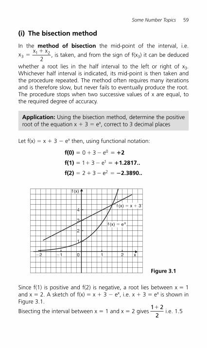
Let f(x) � x � 3 � e x then, using functional notation:
f(0) 2
f(1) 1.2817..
f(2) 2.3890..
� � � �
� � � �
� � � �
0 3
1 3
2 3
0
1
2
e
e
e
�
�
�
0
4
3
2
1
f (x)
x�1�2 1 2
f (x) � ex
f (x) � x � 3
Figure 3.1
Since f(1) is positive and f(2) is negative, a root lies between x � 1 and x � 2. A sketch of f(x) � x � 3 � e x, i.e. x � 3 � ex is shown in Figure 3.1 .
Bisecting the interval between x � 1 and x � 2 gives 1 2
2�
i.e. 1.5
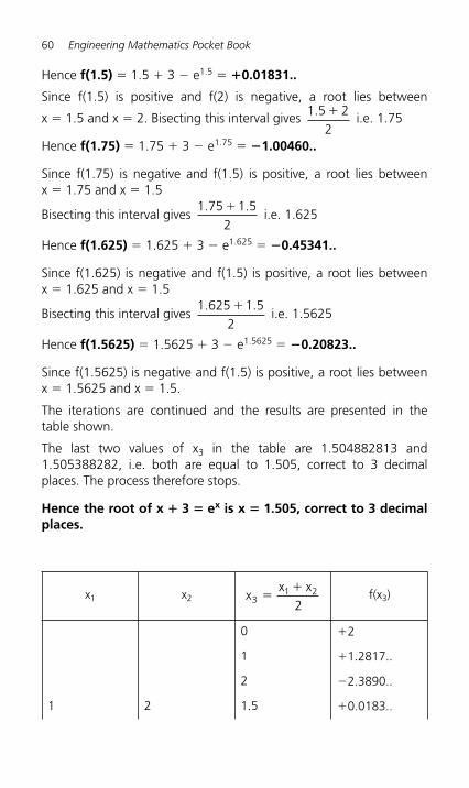
60 Engineering Mathematics Pocket Book
Hence f(1.5) � 1.5 � 3 � e 1.5 � � 0.01831..
Since f(1.5) is positive and f(2) is negative, a root lies between
x � 1.5 and x � 2. Bisecting this interval gives 1 5 22
. �
i.e. 1.75
Hence f(1.75) � 1.75 � 3 � e 1.75 � � 1.00460..
Since f(1.75) is negative and f(1.5) is positive, a root lies between x � 1.75 and x � 1.5
Bisecting this interval gives 1 75 1 5
2. .�
i.e. 1.625
Hence f(1.625) � 1.625 � 3 � e 1.625 � � 0.45341..
Since f(1.625) is negative and f(1.5) is positive, a root lies between x � 1.625 and x � 1.5
Bisecting this interval gives 1 625 1 5
2. .�
i.e. 1.5625
Hence f(1.5625) � 1.5625 � 3 � e 1.5625 � � 0.20823..
Since f(1.5625) is negative and f(1.5) is positive, a root lies between x � 1.5625 and x � 1.5.
The iterations are continued and the results are presented in the table shown.
The last two values of x3 in the table are 1.504882813 and 1.505388282, i.e. both are equal to 1.505, correct to 3 decimal places. The process therefore stops.
Hence the root of x � 3 � e x is x � 1.505, correct to 3 decimal places.
x 1 x2 x
x x3
1 2
2�
�
f(x 3 )
0 � 2
1 � 1.2817..
2 � 2.3890..
1 2 1.5 � 0.0183..
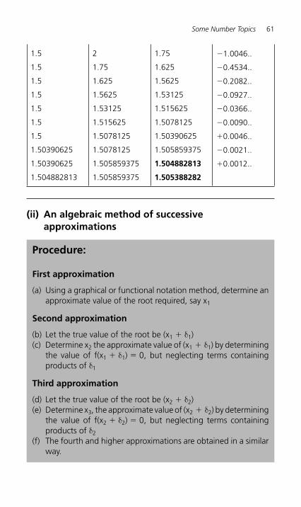
Some Number Topics 61
1.5 2 1.75 � 1.0046..
1.5 1.75 1.625 � 0.4534..
1.5 1.625 1.5625 � 0.2082..
1.5 1.5625 1.53125 � 0.0927..
1.5 1.53125 1.515625 � 0.0366..
1.5 1.515625 1.5078125 � 0.0090..
1.5 1.5078125 1.50390625 � 0.0046..
1.50390625 1.5078125 1.505859375 � 0.0021..
1.50390625 1.505859375 1.504882813 � 0.0012..
1.504882813 1.505859375 1.505388282
(ii) An algebraic method of successive approximations
Procedure:
First approximation
(a) Using a graphical or functional notation method, determine an approximate value of the root required, say x 1
Second approximation
(b) Let the true value of the root be (x 1 � δ 1 ) (c) Determine x 2 the approximate value of (x 1 � δ 1) by determining
the value of f(x 1 � δ 1 ) � 0, but neglecting terms containing products of δ 1
Third approximation
(d) Let the true value of the root be (x 2 � δ 2 ) (e) Determine x 3, the approximate value of (x 2 � δ 2) by d etermining
the value of f(x 2 � δ 2 ) � 0, but neglecting terms containing products of δ 2
(f) The fourth and higher approximations are obtained in a similar way.
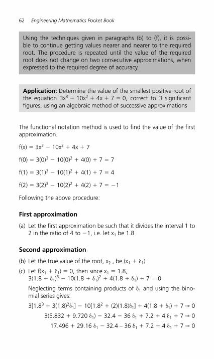
62 Engineering Mathematics Pocket Book
The functional notation method is used to find the value of the first approximation.
f(x) � 3x 3 � 10x 2 � 4x � 7
f(0) � 3(0) 3 � 10(0) 2 � 4(0) � 7 � 7
f(1) � 3(1) 3 � 10(1) 2 � 4(1) � 7 � 4
f(2) � 3(2) 3 � 10(2) 2 � 4(2) � 7 � � 1
Following the above procedure:
First approximation
(a) Let the first approximation be such that it divides the interval 1 to 2 in the ratio of 4 to � 1, i.e. let x 1 be 1.8
Second approximation
(b) Let the true value of the root, x 2 , be (x 1 � δ 1 )
(c) Let f(x 1 � δ 1 ) � 0, then since x 1 � 1.8, 3(1.8 � δ 1 ) 3 � 10(1.8 � δ 1 ) 2 � 4(1.8 � δ 1 ) � 7 � 0
Neglecting terms containing products of δ 1 and using the bino-mial series gives:
3[1.83 � 3(1.8)2 δ 1] � 10[1.82 � (2)(1.8)δ 1] � 4(1.8 � δ 1) � 7 � 0
3(5.832 � 9.720 δ 1) � 32.4 � 36 δ 1 � 7.2 � 4 δ 1 � 7 � 0
17.496 � 29.16 δ 1 � 32.4 – 36 δ 1 � 7.2 � 4 δ 1 � 7 � 0
Using the techniques given in paragraphs (b) to (f), it is possi-ble to continue getting values nearer and nearer to the required root. The procedure is repeated until the value of the required root does not change on two consecutive approximations, when expressed to the required degree of accuracy.
Application: Determine the value of the smallest positive root of the equation 3x 3 � 10x 2 � 4x � 7 � 0, correct to 3 significant figures, using an algebraic method of successive approximations
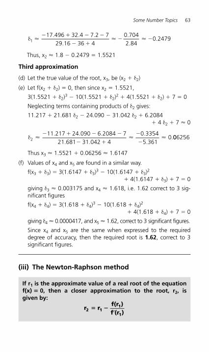
Some Number Topics 63
δ117 496 32 4 7 2 7
29 16 36 40 7042 84
� � �� � � �
� �� �
. . ..
..
0.2479
Thus, x 2 � 1.8 � 0.2479 � 1.5521
Third approximation
(d) Let the true value of the root, x 3 , be (x 2 � δ 2 )
(e) Let f(x 2 � δ 2 ) � 0, then since x 2 � 1.5521,
3(1.5521 � δ 2 ) 3 � 10(1.5521 � δ 2 ) 2 � 4(1.5521 � δ 2 ) � 7 � 0
Neglecting terms containing products of δ 2 gives:
11.217 � 21.681 δ 2 � 24.090 � 31.042 δ 2 � 6.2084 � 4 δ 2 � 7 � 0
δ211 217 24 090 6 2084 7
21 681 31 042 40 33545 361
0� � �� � � �
� �
�
�
. . .. .
..
.006256
Thus x 3 � 1.5521 � 0.06256 � 1.6147
(f) Values of x 4 and x 5 are found in a similar way.
f(x 3 � δ 3 ) � 3(1.6147 � δ 3 ) 3 � 10(1.6147 � δ 3 ) 2 � 4(1.6147 � δ 3 ) � 7 � 0
giving δ 3 � 0.003175 and x 4 � 1.618, i.e. 1.62 correct to 3 sig-nificant figures
f(x 4 � δ 4 ) � 3(1.618 � δ 4 ) 3 � 10(1.618 � δ 4 ) 2 � 4(1.618 � δ 4 ) � 7 � 0
giving δ 4 � 0.0000417, and x 5 � 1.62, correct to 3 significant figures.
Since x 4 and x 5 are the same when expressed to the required degree of accuracy, then the required root is 1.62, correct to 3 significant figures.
(iii) The Newton-Raphson method
If r 1 is the approximate value of a real root of the equationf(x) � 0, then a closer approximation to the root, r 2, is given by:
r rf(r )f (r )2 1
1
1� �
�
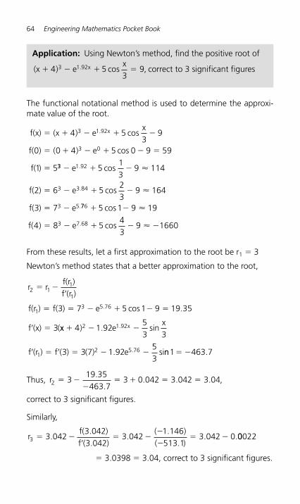
64 Engineering Mathematics Pocket Book
The functional notational method is used to determine the approxi-mate value of the root.
f(x) (x ) ex
f( ) ( ) e
f( )
x� � � � �
� � � � � �
�
4 53
9
0 0 4 5 0 9 59
1 5
3 1 92
3 0
. cos
cos
33 1 92
3 84
3 5
513
9 114
2 523
9 164
3 7
� � �
� � � �
� �
e
f( ) 6 e
f( ) e
3
.
.
.
cos
cos
�
�
776
3 7 68
5 1 9 19
4 8 543
9 1660
� �
� � � � �
cos
cos.
�
�f( ) e
From these results, let a first approximation to the root be r 1 � 3
Newton’s method states that a better approximation to the root,
r rf(r )f (r )
f(r ) f( ) e 1 9
f (x) (
2 11
1
13 5 763 7 5 19 35
3
� ��
� � � � � �
� �
. cos .
xx ) ex
f (r ) f ( ) ( ) e
x� � �
� � � � � �
4 1 9253 3
3 3 7 1 9253
2 1 92
12 5 76
. sin
. si
.
. nn .1 463 7� �
Thus, r 3 0.042 3.042 3.042 319 35463 7
� ��
� � � �.
. ,
correct to 3 significant figures.
Similarly,
r 3.042f( )f ( )
( )( )3
3 0423 042
3 0421 146513 1
3 042 0� ��
� ��
�� �
..
..
.. .00022
� 3.0398 � 3.04, correct to 3 significant figures.
Application: Using Newton’s method, find the positive root of
(x ) e 5xx� � � �43
93 1 92. cos , correct to 3 significant figures
Some Number Topics 65
Since r 2 and r 3 are the same when expressed to the required degree of accuracy, then the required root is 3.04, correct to 3 significant figures.
3.7 Computer numbering systems
Conversion of binary to decimal
Application: Change the binary number 1101.1 to its equivalent decimal form
1101 1 1 2 1 2 0 2 2 1 2
8 4 0 112
13 5
3 2 1 0 1.
.
� � � � � � � � � �
� � � � �
�1
, that is
i.e. 1101.12 � 13.5 10, the suffixes 2 and 10 denoting binary and decimal systems of numbers respectively.
Application: Convert 101.0101 2 to a decimal number
101 0101 1 2 0 2 1 2 0 2
1 2 0 2 1 2
4 0 1
22 1 0 1
2 3 4
. � � � � � � � �
� � � � � �
� � � �
�
� � �
00 0 25 0 0 0625� � � �. . 5.312510
Conversion of decimal to binary
An integer decimal number can be converted to a corresponding binary number by repeatedly dividing by 2 and noting the remainder at each stage, as shown below.
Application: Change 39 10 into binary
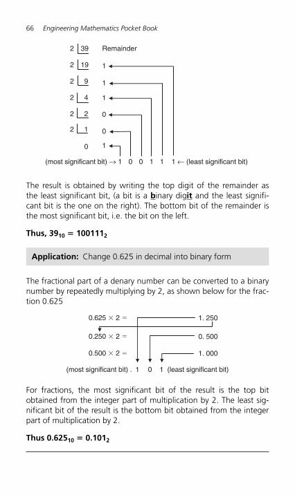
66 Engineering Mathematics Pocket Book
2 39 Remainder
2 19 1
2 9 1
2 4 1
2 2 0
2 1 0
0 1
(most significant bit) → 1 0 0 1 1 1 ← (least significant bit)
The result is obtained by writing the top digit of the remainder as the least significant bit, (a bit is a binary dig it and the least signifi-cant bit is the one on the right). The bottom bit of the remainder is the most significant bit, i.e. the bit on the left.
Thus, 39 10 � 100111 2
Application: Change 0.625 in decimal into binary form
The fractional part of a denary number can be converted to a binary number by repeatedly multiplying by 2, as shown below for the frac-tion 0.625
0.625 � 2 � 1. 250
0.250 � 2 � 0. 500
0.500 � 2 � 1. 000
(most significant bit) . 1 0 1 (least significant bit)
For fractions, the most significant bit of the result is the top bit obtained from the integer part of multiplication by 2. The least sig-nificant bit of the result is the bottom bit obtained from the integer part of multiplication by 2.
Thus 0.625 10 � 0.101 2
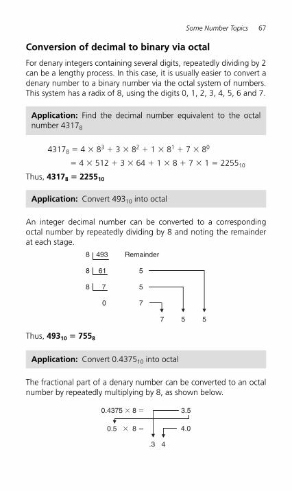
Some Number Topics 67
Conversion of decimal to binary via octal
For denary integers containing several digits, repeatedly dividing by 2 can be a lengthy process. In this case, it is usually easier to convert a denary number to a binary number via the octal system of numbers. This system has a radix of 8, using the digits 0, 1, 2, 3, 4, 5, 6 and 7.
Application: Find the decimal number equivalent to the octal number 4317 8
4317 8 � 4 � 8 3 � 3 � 8 2 � 1 � 8 1 � 7 � 8 0
� 4 � 512 � 3 � 64 � 1 � 8 � 7 � 1 � 2255 10
Thus, 43178 � 2255 10
Application: Convert 493 10 into octal
An integer decimal number can be converted to a corresponding octal number by repeatedly dividing by 8 and noting the remainder at each stage.
8 493 Remainder
8 61 5
8 7 5
0 7
7 5 5
Thus, 49310 � 7558
Application: Convert 0.4375 10 into octal
The fractional part of a denary number can be converted to an octal number by repeatedly multiplying by 8, as shown below.
0.4375 � 8 � 3.5
0.5 � 8 � 4.0
.3 4
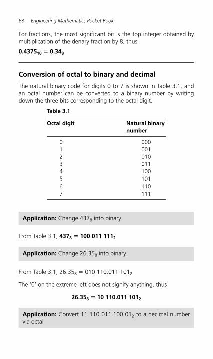
68 Engineering Mathematics Pocket Book
For fractions, the most significant bit is the top integer obtained by multiplication of the denary fraction by 8, thus
0.437510 � 0.34 8
Conversion of octal to binary and decimal
The natural binary code for digits 0 to 7 is shown in Table 3.1 , and an octal number can be converted to a binary number by writing down the three bits corresponding to the octal digit.
Table 3.1
Octal digit Natural binary number
0 000 1 001 2 010 3 011 4 100 5 101 6 110 7 111
Application: Change 437 8 into binary
From Table 3.1 , 4378 � 100 011 111 2
Application: Change 26.35 8 into binary
From Table 3.1 , 26.35 8 � 010 110.011 101 2
The ‘ 0 ’ on the extreme left does not signify anything, thus
26.358 � 10 110.011 101 2
Application: Convert 11 110 011.100 01 2 to a decimal number via octal
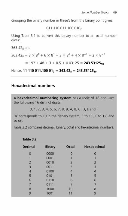
Some Number Topics 69
Grouping the binary number in three’s from the binary point gives:
011 110 011.100 010 2
Using Table 3.1 to convert this binary number to an octal number gives:
363.42 8 and
363.42 8 � 3 � 8 2 � 6 � 8 1 � 3 � 8 0 � 4 � 8 � 1 � 2 � 8 � 2
� 192 � 48 � 3 � 0.5 � 0.03125 � 243.5312510
Hence, 11 110 011.100 01 2 � 363.42 8 � 243.53125 10
Hexadecimal numbers
A hexadecimal numbering system has a radix of 16 and uses the following 16 distinct digits:
0, 1, 2, 3, 4, 5, 6, 7, 8, 9, A, B, C, D, E and F
‘ A’ corresponds to 10 in the denary system, B to 11, C to 12, and so on.
Table 3.2 compares decimal, binary, octal and hexadecimal numbers.
Table 3.2
Decimal Binary Octal Hexadecimal
0 0000 0 01 0001 1 12 0010 2 23 0011 3 34 0100 4 45 0101 5 56 0110 6 67 0111 7 78 1000 10 89 1001 11 9
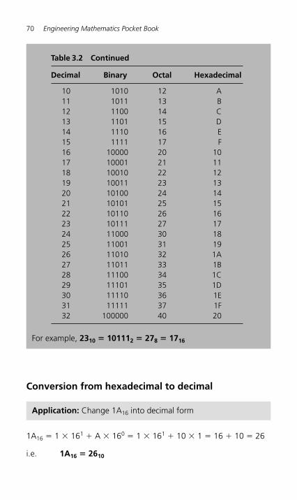
70 Engineering Mathematics Pocket Book
Conversion from hexadecimal to decimal
For example, 2310 � 10111 2 � 27 8 � 17 16
Table 3.2 Continued
Decimal Binary Octal Hexadecimal
10 1010 12 A11 1011 13 B12 1100 14 C13 1101 15 D14 1110 16 E15 1111 17 F16 10000 20 1017 10001 21 1118 10010 22 1219 10011 23 1320 10100 24 1421 10101 25 1522 10110 26 1623 10111 27 1724 11000 30 1825 11001 31 1926 11010 32 1A27 11011 33 1B28 11100 34 1C29 11101 35 1D30 11110 36 1E31 11111 37 1F32 100000 40 20
Application: Change 1A 16 into decimal form
1A 16 � 1 � 16 1 � A � 16 0 � 1 � 16 1 � 10 � 1 � 16 � 10 � 26
i.e. 1A16 � 2610
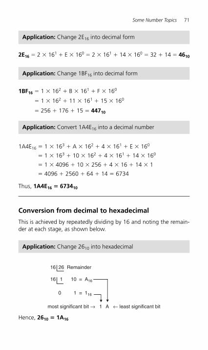
Some Number Topics 71
2E16 � 2 � 161 � E � 160 � 2 � 161 � 14 � 160 � 32 � 14 � 4610
Application: Change 2E 16 into decimal form
Application: Change 1BF 16 into decimal form
1BF16 � 1 � 16 2 � B � 16 1 � F � 16 0
� 1 � 16 2 � 11 � 16 1 � 15 � 16 0
� 256 � 176 � 15 � 44710
Application: Convert 1A4E 16 into a decimal number
1A4E 16 � 1 � 16 3 � A � 16 2 � 4 � 16 1 � E � 16 0
� 1 � 16 3 � 10 � 16 2 � 4 � 16 1 � 14 � 16 0
� 1 � 4096 � 10 � 256 � 4 � 16 � 14 � 1
� 4096 � 2560 � 64 � 14 � 6734
Thus, 1A4E16 � 6734 10
Conversion from decimal to hexadecimal
This is achieved by repeatedly dividing by 16 and noting the remain-der at each stage, as shown below.
Application: Change 26 10 into hexadecimal
16 26 Remainder
16 1 10 ≡ A16
0 1 ≡ 116
most significant bit → 1 A ← least significant bit
Hence, 2610 � 1A 16
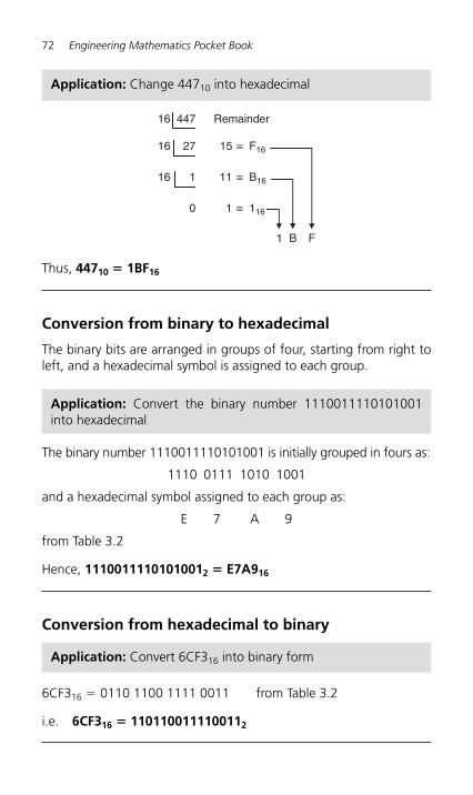
72 Engineering Mathematics Pocket Book
16 447 Remainder
16 27 15 ≡ F16
16 1 11 ≡ B16
0 1 ≡ 116
1 B F
Thus, 44710 � 1BF 16
Conversion from binary to hexadecimal
The binary bits are arranged in groups of four, starting from right to left, and a hexadecimal symbol is assigned to each group.
Application: Convert the binary number 1110011110101001 into hexadecimal
The binary number 1110011110101001 is initially grouped in fours as:
1110 0111 1010 1001
and a hexadecimal symbol assigned to each group as:
E 7 A 9
from Table 3.2
Hence, 11100111101010012 � E7A9 16
Conversion from hexadecimal to binary
Application: Convert 6CF3 16 into binary form
6CF3 16 � 0110 1100 1111 0011 from Table 3.2
i.e. 6CF316 � 110110011110011 2
Application: Change 447 10 into hexadecimal
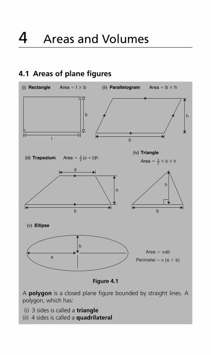
4 Areas and Volumes
4.1 Areas of plane figures
A polygon is a closed plane figure bounded by straight lines. A polygon, which has:
(i) 3 sides is called a triangle (ii) 4 sides is called a quadrilateral
b
a
h
b
h
b
h
bArea � �ab
Perimeter ≈ � (a � b)a
l
b
(i) Rectangle Area � I � b (ii) Parallelogram Area � b � h
(iii) Area ( )12Trapezium � �a hb
(iv)
Area 12
Triangle
� � �b h
(v) Ellipse
Figure 4.1
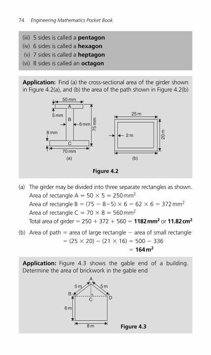
74 Engineering Mathematics Pocket Book
(iii) 5 sides is called a pentagon (iv) 6 sides is called a hexagon (v) 7 sides is called a heptagon (vi) 8 sides is called an octagon
(a) The girder may be divided into three separate rectangles as shown. Area of rectangle A � 50 � 5 � 250 mm 2 Area of rectangle B � (75 � 8 � 5) � 6 � 62 � 6 � 372 mm 2 Area of rectangle C � 70 � 8 � 560 mm 2 Total area of girder � 250 � 372 � 560 � 1182 mm2 or 11.82 cm2
(b) Area of path � area of large rectangle � area of small rectangle � (25 � 20) � (21 � 16) � 500 � 336
� 164 m2
Application: Find (a) the cross-sectional area of the girder shown in Figure 4.2(a) , and (b) the area of the path shown in Figure 4.2(b)
2 m
25 m
20 m
(b)
50 mm
5 mm
A
B
C
8 mm
6 mm
75 m
m
70 mm
(a)
Figure 4.2
Application: Figure 4.3 shows the gable end of a building. Determine the area of brickwork in the gable end
5 m 5 m
6 m
BC
A
D
8 m Figure 4.3
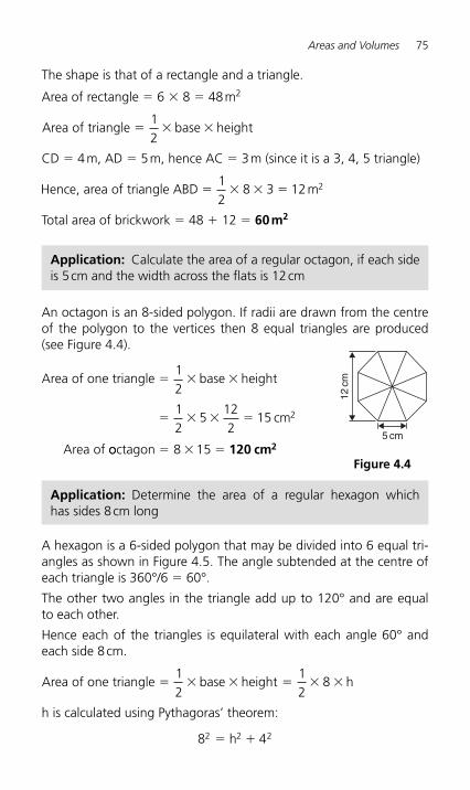
Areas and Volumes 75
The shape is that of a rectangle and a triangle.
Area of rectangle � 6 � 8 � 48 m 2
Area of triangle base height� � �
12
CD � 4 m, AD � 5 m, hence AC � 3 m (since it is a 3, 4, 5 triangle)
Hence, area of triangle ABD 8 3 12m2� � � �
12
Total area of brickwork � 48 � 12 � 60 m 2
12 c
m
5 cm
Figure 4.4
Application: Calculate the area of a regular octagon, if each side is 5 cm and the width across the flats is 12 cm
An octagon is an 8-sided polygon. If radii are drawn from the centre of the polygon to the vertices then 8 equal triangles are produced (see Figure 4.4 ).
Area of one triangle base height
5 cm
Area of
� � �
� � � �
12
12
122
15 2
ooctagon 8 15� � � 120 cm2
A hexagon is a 6-sided polygon that may be divided into 6 equal tri-angles as shown in Figure 4.5 . The angle subtended at the centre of each triangle is 360°/6 � 60°.
The other two angles in the triangle add up to 120° and are equal to each other.
Hence each of the triangles is equilateral with each angle 60° and each side 8 cm.
Area of one triangle base height 8 h� � � � � �
12
12
h is calculated using Pythagoras ’ theorem:
8 42 2 2� �h
Application: Determine the area of a regular hexagon which has sides 8 cm long
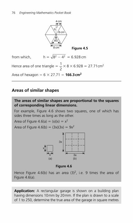
76 Engineering Mathematics Pocket Book
from which, h cm� � �8 4 6 9282 2 .
Hence area of one triangle 8 cm� � � �
12
6 928 27 71 2. .
Area of hexagon � 6 � 27.71 � 166.3 cm 2
Areas of similar shapes
4 cm
8 cm
8 cm
h
60°
Figure 4.5
The areas of similar shapes are proportional to the squares of corresponding linear dimensions.
For example, Figure 4.6 shows two squares, one of which has sides three times as long as the other.
Area of Figure 4.6(a) � (x)(x) � x 2
Area of Figure 4.6(b) � (3x)(3x) � 9x2
Hence Figure 4.6(b) has an area (3) 2, i.e. 9 times the area of Figure 4.6(a) .
Figure 4.6
(a)x
x
3x
(b)3x
Application: A rectangular garage is shown on a building plan having dimensions 10 mm by 20 mm. If the plan is drawn to a scale of 1 to 250, determine the true area of the garage in square metres
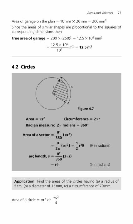
Areas and Volumes 77
Area of garage on the plan � 10 mm � 20 mm � 200 mm 2
Since the areas of similar shapes are proportional to the squares of corresponding dimensions then
true area of garage
1
� � � �
��
�
200 250 12 5 10
12 5 1010
2 6 2
6
62
( ) .
.
mm
m 22.5 m2
4.2 Circles
Area � π r 2 Circumference � 2 π r
Radian measure: 2 π radians � 360°
Area of a sector360
( r )
2( r )
12
r
ar
2
2 2
��
� �
θπ
θπ
π θ ( in radians)θ
cc length, s360
(2 r)
r
��
�
θπ
θ ( in radians)θ
r
r
s
�
Figure 4.7
Application: Find the areas of the circles having (a) a radius of 5 cm, (b) a diameter of 15 mm, (c) a circumference of 70 mm
Area of a circle r or
d� π
π22
4
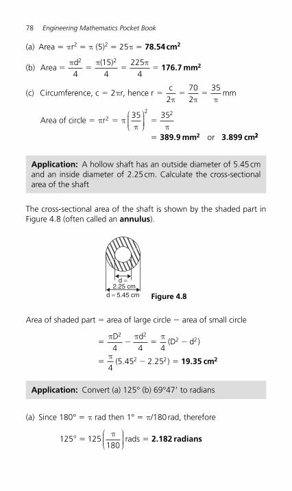
78 Engineering Mathematics Pocket Book
(a) Area � π r 2 � π (5) 2 � 25 π � 78.54 cm 2
(b) Area
d ( )� � � �
π π π2 2
4154
2254
176.7 mm2
(c) Circumference, c 2 r, hence rc
mm� � � �ππ π π2
702
35
Area of circle r� � �
�
π ππ π
22 235 35⎛
⎝⎜⎜⎜
⎞⎠⎟⎟⎟⎟
389.9 mm 3.899 cm2 or 22
Application: A hollow shaft has an outside diameter of 5.45 cm and an inside diameter of 2.25 cm. Calculate the cross-sectional area of the shaft
The cross-sectional area of the shaft is shown by the shaded part in Figure 4.8 (often called an annulus ).
2.25 cm d = 5.45 cm
d =
Figure 4.8
Area of shaded part � area of large circle � area of small circle
� � � �
� � �
π π π
π
D d(D d )
( )
2 22 2
2 2
4 4 4
45 45 2 25. . 19.35 cm2
Application: Convert (a) 125° (b) 69°47 � to radians
(a) Since 180° � π rad then 1° � π /180 rad, therefore
125 125180
°⎛⎝⎜⎜⎜
⎞⎠⎟⎟⎟⎟� �
πrads 2.182 radians
Areas and Volumes 79
(b) 69 47°
°°� � �69
4760
69 783.
69 783 69 783180
. .°⎛⎝⎜⎜⎜
⎞⎠⎟⎟⎟⎟� �
π1.218 radians
Application: Convert (a) 0.749 radians, (b) 3 π/4 radians, to degrees and minutes
(a) Since π rad � 180° then 1 rad � 180 ° / π , therefore
0 749 0 749180
42 915. . .��
� �π
⎛⎝⎜⎜⎜
⎞⎠⎟⎟⎟⎟
0.915° � (0.915 � 60) � � 55 � , correct to the nearest minute,
hence 0.749 radians 42 55� � �
(b)
Since 1 rad
then rad
��
�
180
34
34
180
π
π ππ
⎛⎝⎜⎜⎜
⎞⎠⎟⎟⎟⎟
⎛⎝⎜⎜⎜
⎞⎠⎟⎟⎟⎟⎟�
� � �34
180( ) 135�
Application: Find the length of arc of a circle of radius 5.5 cm when the angle subtended at the centre is 1.20 radians
Length of arc, s � r θ , where θ is in radians, hence
s � (5.5)(1.20) � 6.60 cm
Application: Determine the diameter and circumference of a cir-cle if an arc of length 4.75 cm subtends an angle of 0.91 radians
Since s r then r
scm� � � �θ
θ4 750 91
5 22..
.
Diameter � 2 � radius � 2 � 5.22 � 10.44 cm
Circumference, c � π d � π (10.44) � 32.80 cm
Application: Determine the angle, in degrees and minutes, sub-tended at the centre of a circle of diameter 42 mm by an arc of length 36 mm and the area of the minor sector formed
80 Engineering Mathematics Pocket Book
Since length of arc, s � r θ then θ � s/r
Radius, r
diameter21mm� � �
2422
hence
sr
radians� � � �3621
1 7143.
1.7143 rad � 1.7143 � (180/ π )° � 98.22° � 98 ° 13 �
� angle subtended at centre of circle
Area of sector � � �
12
12
21 1 71432 2r ( ) ( )θ . 378 mm2
Application: A football stadium floodlight can spread its illumi-nation over an angle of 45° to a distance of 55 m. Determine the maximum area that is floodlit
Floodlit area � � � �area of sector r12
( )12
55 45180
2 2θπ⎛
⎝⎜⎜⎜
⎞⎠⎟⎟⎟⎟⎟
� 1188 m2
Application: An automatic garden spray produces a spray to a distance of 1.8 m and revolves through an angle α which may be varied. If the desired spray catchment area is to be 2.5 m 2, deter-mine the required angle α , correct to the nearest degree
Area of sector r , hence ( )� �
12
2 512
1 82 2θ α. .
from which, radiansα �
��
2 5 21 8
1 54322
..
.
1 5432 1 5432180
88 42. . .rad � ��
� �π
⎛⎝⎜⎜⎜
⎞⎠⎟⎟⎟⎟
Hence angle α � 88° , correct to the nearest degree.
Application: The angle of a tapered groove is checked using a 20 mm diameter roller as shown in Figure 4.9 . If the roller lies 2.12 mm below the top of the groove, determine the value of angle θ
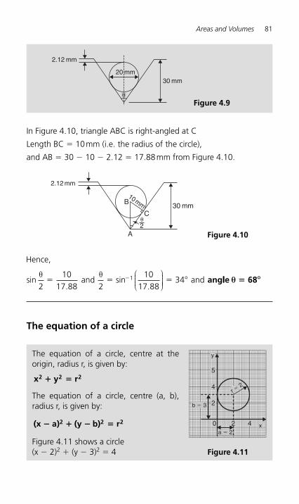
Areas and Volumes 81
In Figure 4.10 , triangle ABC is right-angled at C
Length BC � 10 mm (i.e. the radius of the circle),
and AB � 30 � 10 � 2.12 � 17.88 mm from Figure 4.10 .
2.12 mm
10mm
�2
30 mm
A
B
C
Figure 4.10
2.12 mm
20 mm30 mm
�
Figure 4.9
Hence,
and andsin.
sin.
θ θ2
1017 88 2
1017 88
341� � ��⎛⎝⎜⎜⎜
⎞⎠⎟⎟⎟⎟ ° anglle 68θ °�
The equation of a circle
The equation of a circle, centre at the origin, radius r, is given by:
x y r2 2 2� �
The equation of a circle, centre (a, b), radius r, is given by:
(x a) (y b) r2 2 2� � � �
Figure 4.11 shows a circle(x � 2) 2 � (y � 3) 2 � 4
4
5
2
0 2 4
b � 3
a � 2
r � 2
y
x
Figure 4.11
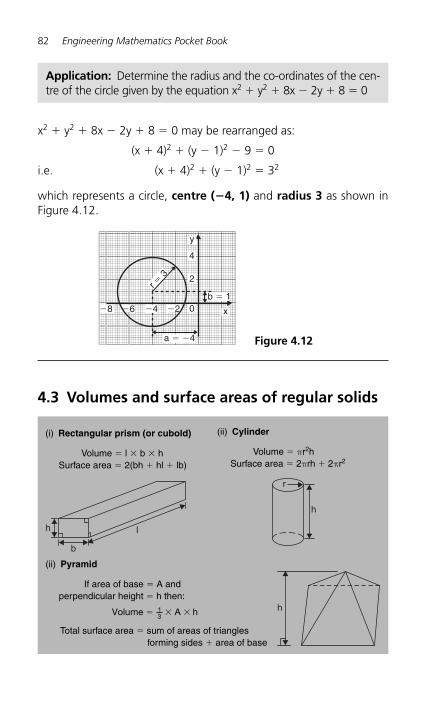
82 Engineering Mathematics Pocket Book
x 2 � y 2 � 8x � 2y � 8 � 0 may be rearranged as:
(x � 4) 2 � (y � 1) 2 � 9 � 0
i.e. (x � 4) 2 � (y � 1) 2 � 3 2
which represents a circle, centre ( �4, 1) and radius 3 as shown in Figure 4.12 .
Application: Determine the radius and the co-ordinates of the cen-tre of the circle given by the equation x 2 � y2 � 8x � 2y � 8 � 0
4.3 Volumes and surface areas of regular solids
b
lh
h
r
(i) Rectangular prism (or cubold)
Volume � l � b � hSurface area � 2(bh � hl � lb)
(ii) Cylinder
Volume � πr2hSurface area � 2πrh � 2πr2
(ii) Pyramid
If area of base � A andperpendicular height � h then:
Volume A h13� � �
Total surface area � sum of areas of triangles forming sides � area of base
h
�8 �6 �4 �2 0
2
4
b � 1
a � �4
r � 3
y
x
Figure 4.12
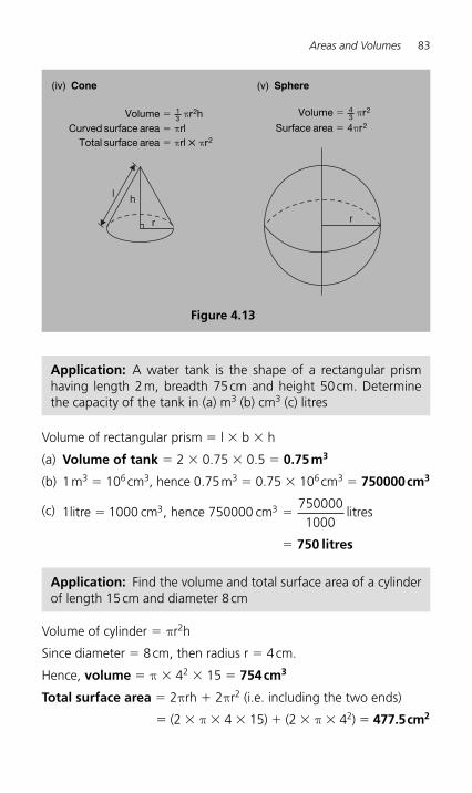
Areas and Volumes 83
Volume of rectangular prism � l � b � h
(a) Volume of tank � 2 � 0.75 � 0.5 � 0.75 m 3
(b) 1 m3 � 106 cm3, hence 0.75 m3 � 0.75 � 106 cm3 � 750000 cm3
(c)
1litre 1000 cm , hence 750000 cm litres3 3� �
�
7500001000
750 litres
l h
r r
(iv) Cone
Volume r hCurved surface area rl
Total surface area rl
13
2� πππ
�
� �� πr2
(v) Sphere
Volume r
Surface area 4 r
43
2
2
� π
π�
Application: A water tank is the shape of a rectangular prism having length 2 m, breadth 75 cm and height 50 cm. Determine the capacity of the tank in (a) m 3 (b) cm 3 (c) litres
Application: Find the volume and total surface area of a cylinderof length 15 cm and diameter 8 cm
Volume of cylinder � π r 2 h
Since diameter � 8 cm, then radius r � 4 cm.
Hence, volume � π � 4 2 � 15 � 754 cm3
Total surface area � 2 π rh � 2 π r 2 (i.e. including the two ends)
� (2 � π � 4 � 15) � (2 � π � 42) � 477.5 cm2
Figure 4.13
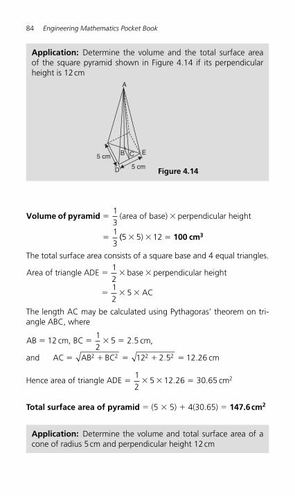
84 Engineering Mathematics Pocket Book
Volume of pyramid � �
�
1313
(area of base) perpendicular height
(( )5 5 12� � � 100 cm3
The total surface area consists of a square base and 4 equal triangles.
Area of triangle ADE base perpendicular height
AC
� � �
� � �
1212
5
The length AC may be calculated using Pythagoras ’ theorem on tri-angle ABC, where
AB 12 cm, BC cm,
and AC AB BC cm
� � � �
� � � � �
12
5 2 5
12 2 5 12 262 2 2 2
.
. .
Hence area of triangle ADE cm� � � �
12
5 12 26 30 65 2. .
Total surface area of pyramid � (5 � 5) � 4(30.65) � 147.6 cm 2
Application: Determine the volume and the total surface area of the square pyramid shown in Figure 4.14 if its perpendicular height is 12 cm
5 cm
A
B C E
D
5 cm
Figure 4.14
Application: Determine the volume and total surface area of a cone of radius 5 cm and perpendicular height 12 cm
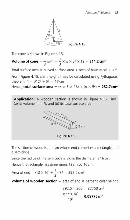
Areas and Volumes 85
The cone is shown in Figure 4.15.
Volume of cone � � � � � �
13
13
5 122 2π πr h 314.2 cm3
Total surface area � curved surface area � area of base � π rl � π r 2
From Figure 4.15 , slant height l may be calculated using Pythagoras ’ theorem: 1 12 5 132 2� � � cm Hence, total surface area � ( π � 5 � 13) � ( π � 5 2 ) � 282.7 cm 2
r � 5 cm
lh �12 cm
Figure 4.15
Application: A wooden section is shown in Figure 4.16 . Find (a) its volume (in m 3 ), and (b) its total surface area
3 m12 cm
r
r � 8 mm
Figure 4.16
The section of wood is a prism whose end comprises a rectangle and a semicircle.
Since the radius of the semicircle is 8 cm, the diameter is 16 cm.
Hence the rectangle has dimensions 12 cm by 16 cm.
Area of end ( 16 cm� � � �12
12
8 292 52 2) .π
Volume of wooden section � area of end � perpendicular height
� � �
� �
292 5 300 87750
8775010
3
3
6
. cm
m0.08775 m3
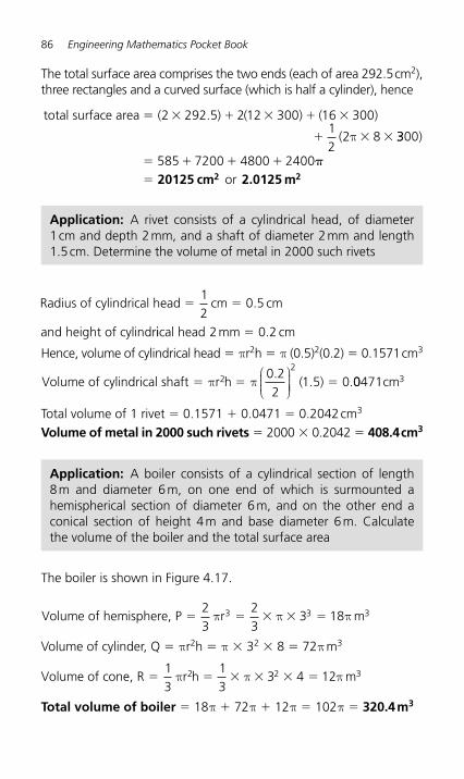
86 Engineering Mathematics Pocket Book
The total surface area comprises the two ends (each of area 292.5 cm2), three rectangles and a curved surface (which is half a cylinder), hence
total surface area ( ) ( ) ( )
(
� � � � � �
� � �
2 292 5 2 12 300 16 30012
2 8
.
π 3300
7200 4800 2400
)
585or
� � � � �
� 20125 cm 2.0125 m2 2
Radius of cylindrical head cm cm
and height of cylindr
� �12
0 5.
iical head mm2 0 2� . cm Hence, volume of cylindrical head � πr2h � π (0.5) 2(0.2) � 0.1571 cm3
Volume of cylindrical shaft r h ( )� � �π π2
20 22
1 5 0.
. .⎛⎝⎜⎜⎜
⎞⎠⎟⎟⎟⎟ 00471 3cm
Total volume of 1 rivet � 0.1571 � 0.0471 � 0.2042 cm 3 Volume of metal in 2000 such rivets � 2000 � 0.2042 � 408.4 cm3
Application: A boiler consists of a cylindrical section of length 8 m and diameter 6 m, on one end of which is surmounted a hemispherical section of diameter 6 m, and on the other end a conical section of height 4 m and base diameter 6 m. Calculate the volume of the boiler and the total surface area
The boiler is shown in Figure 4.17 .
Volume of hemisphere, P r m� � � � �
23
23
3 183 3 3π π π
Volume of cylinder, Q � π r 2 h � π � 3 2 � 8 � 72 π m 3
Volume of cone, R r h m� � � � � �
13
13
3 4 122 2 3π π π
Total volume of boiler � 18 π � 72 π � 12 π � 102 π � 320.4 m3
Application: A rivet consists of a cylindrical head, of diameter 1 cm and depth 2 mm, and a shaft of diameter 2 mm and length 1.5 cm. Determine the volume of metal in 2000 such rivets
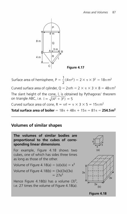
Areas and Volumes 87
Surface area of hemisphere, P ( r ) m� � � � �
12
4 2 3 182 2 2π π π
Curved surface area of cylinder, Q � 2πrh � 2 � π � 3 � 8 � 48π m2
The slant height of the cone, l, is obtained by Pythagoras ’ theorem on triangle ABC, i.e. l ( )� � �4 3 52 2
Curved surface area of cone, R � π rl � π � 3 � 5 � 15 π m 2
Total surface area of boiler � 18π � 48π � 15π � 81π � 254.5 m2
Volumes of similar shapes
4 m
3 m
P
Q
I
C
R
BA
8 m
6 m
Figure 4.17
The volumes of similar bodies are proportional to the cubes of corre-sponding linear dimensions .
For example, Figure 4.18 shows two cubes, one of which has sides three times as long as those of the other.
Volume of Figure 4.18(a) � (x)(x)(x) � x 3
Volume of Figure 4.18(b) � (3x)(3x)(3x) � 27x3
Hence Figure 4.18(b) has a volume (3) 3 , i.e. 27 times the volume of Figure 4.18(a) .
(a)
x
xx
Figure 4.18
3x
3x
3x
(b)
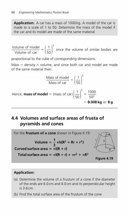
88 Engineering Mathematics Pocket Book
Volume of modelVolume of car
�1
50
3⎛⎝⎜⎜⎜
⎞⎠⎟⎟⎟⎟
since the volume of similar bodies are
proportional to the cube of corresponding dimensions.
Mass � density � volume, and since both car and model are made of the same material then:
Mass of modelMass of car
�1
50
3⎛⎝⎜⎜⎜
⎞⎠⎟⎟⎟⎟
Hence, of carmass of model � �
�
( )mass1
50100050
3
3
⎛⎝⎜⎜⎜
⎞⎠⎟⎟⎟⎟
00.008 kg 8 gor
4.4 Volumes and surface areas of frusta of pyramids and cones
Application: A car has a mass of 1000 kg. A model of the car is made to a scale of 1 to 50. Determine the mass of the model if the car and its model are made of the same material
For the frustum of a cone shown in Figure 4.19 :
Volume13
h(R Rr r )
Curved surface area l(R r)
Total surf
2 2� � �
� �
π
π
aace area l(R r) r R2 2� � � �π π π
r
hI
R
Figure 4.19
Application:
(a) Determine the volume of a frustum of a cone if the diameter of the ends are 6.0 cm and 4.0 cm and its perpendicular height is 3.6 cm.
(b) Find the total surface area of the frustum of the cone
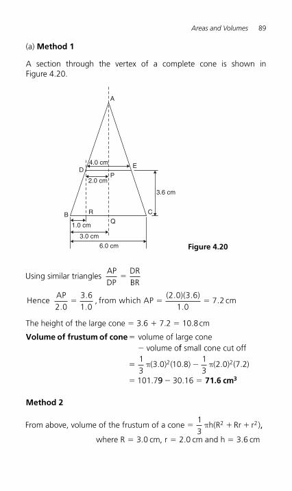
Areas and Volumes 89
(a) Method 1
A section through the vertex of a complete cone is shown in Figure 4.20 .
4.0 cm
2.0 cm
3.0 cm
6.0 cm
3.6 cm
RQ
CB
DE
P
A
1.0 cm
Figure 4.20
Using similar triangles
APDP
DRBR
�
Hence
APfrom which AP
( )( )cm
2 03 61 0
2 0 3 61 0
7 2.
.
.,
. ..
.� � �
The height of the large cone � 3.6 � 7.2 � 10.8 cm
Volume of frustum of cone � �
volume of large conevolume off small cone cut off
( ) ( ) ( ) ( )� �
�
13
3 0 10 813
2 0 7 2
101 7
2 2π π. . . .
. 99 30 16� �. 71.6 cm3
Method 2
From above, volume of the frustum of a cone h(R Rr r )� � �13
2 2π ,,
where R cm, r cm and h cm� � �3 0 2 0 3 6. . .
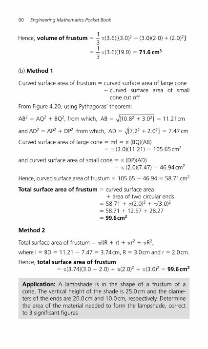
90 Engineering Mathematics Pocket Book
Hence, ( )[( ) ( )( ) ( )volume of frustum � � �13
3 6 3 0 3 0 2 0 2 02 2π . . . . . ]]
( )( )� �13
3 6 19 0π . . 71.6 cm3
(b) Method 1
Curved surface area of frustum � curved surface area of large cone � curved surface area of small
cone cut off
From Figure 4.20 , using Pythagoras ’ theorem:
AB 2 � AQ 2 � BQ 2 , from which, AB [ ] cm� � �10 8 3 0 11 212 2. . .
and AD 2 � AP2 � DP2, from which, AD [ 2.0 ] cm2� � �7 2 7 472. .
Curved surface area of large cone � π rl � π (BQ)(AB) � π (3.0)(11.21) � 105.65 cm 2
and curved surface area of small cone � π (DP)(AD) � π (2.0)(7.47) � 46.94 cm 2
Hence, curved surface area of frustum � 105.65 � 46.94 � 58.71 cm2
Total surface area of frustum � curved surface area � area of two circular ends
� 58.71 � π (2.0) 2 � π (3.0) 2 � 58.71 � 12.57 � 28.27 � 99.6 cm2
Method 2
Total surface area of frustum � π l(R � r) � π r 2 � π R 2 ,
where l � BD � 11.21 � 7.47 � 3.74 cm, R � 3.0 cm and r � 2.0 cm.
Hence, total surface area of frustum � π (3.74)(3.0 � 2.0) � π (2.0) 2 � π (3.0) 2 � 99.6 cm2
Application: A lampshade is in the shape of a frustum of a cone. The vertical height of the shade is 25.0 cm and the diame-ters of the ends are 20.0 cm and 10.0 cm, respectively. Determine the area of the material needed to form the lampshade, correct to 3 significant figures
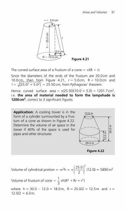
Areas and Volumes 91
r � 5.0 cm
R � 10.0 cm
h�
25.
0 cm
5.0 cm
I
Figure 4.21
Volume of cylindrical protion r h (� �π π2
225 0
212 0
..
⎛⎝⎜⎜⎜
⎞⎠⎟⎟⎟⎟ )) m� 5890 3
Volume of frustum of cone h(R Rr r )� � �
13
2 2π
where h � 30.0 � 12.0 � 18.0 m, R � 25.0/2 � 12.5 m and r � 12.0/2 � 6.0 m.
Application: A cooling tower is in the form of a cylinder surmounted by a frus-tum of a cone as shown in Figure 4.22 . Determine the volume of air space in the tower if 40% of the space is used for pipes and other structures
12.0 m
25.0 m
12.0
m 30.0
m
Figure 4.22
The curved surface area of a frustum of a cone � π l(R � r)
Since the diameters of the ends of the frustum are 20.0 cm and 10.0 cm, then from Figure 4.21 , r � 5.0 cm, R � 10.0 cm and l [ ] cm� � �25 0 5 0 25 502 2. . . , from Pythagoras ’ theorem.
Hence curved surface area � π(25.50)(10.0 � 5.0) � 1201.7 cm2 , i.e. the area of material needed to form the lampshade is 1200 cm2 , correct to 3 significant figures.
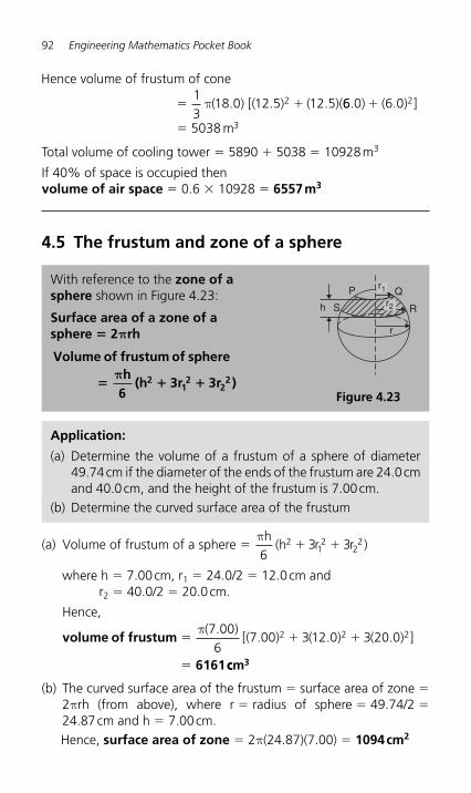
92 Engineering Mathematics Pocket Book
Hence volume of frustum of cone
( ) [( ) ( )(� �13
18 0 12 5 12 52π . . . 66 0 6 0
5038
2. .) ( ) ]
m3
�
� Total volume of cooling tower � 5890 � 5038 � 10928 m 3
If 40% of space is occupied then volume of air space � 0.6 � 10928 � 6557 m3
4.5 The frustum and zone of a sphere
With reference to the zone of a sphere shown in Figure 4.23 :
Surface area of a zone of a sphere � 2 π rh
Volume of frustum of sphereh
6(h 3r 3r )2
12
22� � �
π
r2
r1
R
QP
Sh
r
Figure 4.23
Application:
(a) Determine the volume of a frustum of a sphere of diameter 49.74 cm if the diameter of the ends of the frustum are 24.0 cm and 40.0 cm, and the height of the frustum is 7.00 cm.
(b) Determine the curved surface area of the frustum
(a) Volume of frustum of a sphere
h(h r r )� � �
π6
3 3212
22
where h � 7.00 cm, r 1 � 24.0/2 � 12.0 cm and r 2 � 40.0/2 � 20.0 cm.
Hence,
volume of frustum
6161
� � �
�
π( )[( ) ( ) ( ) ]
7 006
7 00 3 12 0 3 20 02 2 2.. . .
ccm3
(b) The curved surface area of the frustum � surface area of zone � 2 πrh (from above), where r � radius of sphere � 49.74/2 � 24.87 cm and h � 7.00 cm. Hence, surface area of zone � 2 π (24.87)(7.00) � 1094 cm2
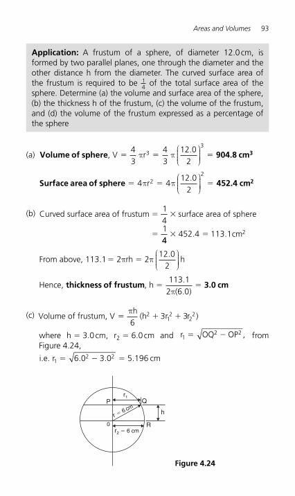
Areas and Volumes 93
(a) Volume of sphere 904.8 cm3, V r� � �
43
43
12 02
33
π π.⎛
⎝⎜⎜⎜
⎞⎠⎟⎟⎟⎟
Surface area of sphere 452.4 cm2� � �4 4
12 02
22
π πr.⎛
⎝⎜⎜⎜
⎞⎠⎟⎟⎟⎟
(b)
Curved surface area of frustum surface area of sphere� �
�
14144
452 4 113 1 2� �. . cm
From above, 113.1 rh h� �2 2
12 02
π π.⎛
⎝⎜⎜⎜
⎞⎠⎟⎟⎟⎟
Hence, , h
( )thickness of frustum 3.0 cm� �
113 12 6 0
.
.π
(c) Volume of frustum, V
h(h 3r r )� � �
π6
3212
22
where h � 3.0 cm, r 2 � 6.0 cm and r OQ OP ,1
2 2� � from Figure 4.24,
i.e. r cm12 26 0 3 0 5 196� � �. . .
Application: A frustum of a sphere, of diameter 12.0 cm, is formed by two parallel planes, one through the diameter and the other distance h from the diameter. The curved surface area of the frustum is required to be 1
4 of the total surface area of the
sphere. Determine (a) the volume and surface area of the sphere, (b) the thickness h of the frustum, (c) the volume of the frustum, and (d) the volume of the frustum expressed as a percentage of the sphere
0r2 � 6 cm
r1
r � 6 cmh
Q
R
P
Figure 4.24
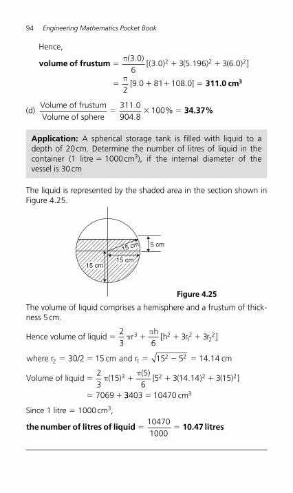
94 Engineering Mathematics Pocket Book
Application: A spherical storage tank is filled with liquid to a depth of 20 cm. Determine the number of litres of liquid in the container (1 litre � 1000 cm 3), if the internal diameter of the vessel is 30 cm
5 cm
15 cm15 cm
15 cm
Figure 4.25
The liquid is represented by the shaded area in the section shown in Figure 4.25 .
Hence,
volume of frustum � � �
�
π
π
( )[( ) ( ) ( ) ]
[
3 06
3 0 3 5 196 3 6 0
29 0
2 2 2.. . .
. �� � �81 108 0. ] 311.0 cm3
(d)
Volume of frustumVolume of sphere
%� � �311 0904 8
100..
34.37%
The volume of liquid comprises a hemisphere and a frustum of thick-ness 5 cm.
Hence volume of liquid r
h[h r r ]� � � �
23 6
3 33 212
22π
π
where r 30/2 15 cm and r cm2 � � � � �12 215 5 14 14.
Volume of liquid ( )( )
[ ( ) ( ) ]� � � �
� �
23
155
65 3 14 14 3 15
7069
3 2 2 2ππ
.
33403 10470 3� cm Since 1 litre � 1000 cm 3 ,
the number of litres of liquid 10.47 litres� �104701000
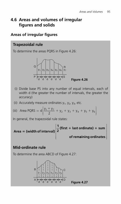
Areas and Volumes 95
4.6 Areas and volumes of irregular figures and solids
Areas of irregular figures
Trapezoidal rule
To determine the areas PQRS in Figure 4.26 :
(i) Divide base PS into any number of equal intervals, each of width d (the greater the number of intervals, the greater the accuracy)
(ii) Accurately measure ordinates y 1 , y 2 , y 3 , etc.
(iii) Area PQRS d
y yy y y y y=
⎡
⎣⎢⎢
⎤
⎦⎥⎥
1 72 3 4 5 62
�� � � � �
In general, the trapezoidal rule states:
Area (width of interval)
12
(first last ordinate) sum
of rem
�� �
aaining ordinates
⎡
⎣
⎢⎢⎢⎢⎢
⎤
⎦
⎥⎥⎥⎥⎥
Mid-ordinate rule
To determine the area ABCD of Figure 4.27 :
y1 y2 y3 y4 y5 y6 y7
d d d d d dS
RQ
P Figure 4.26
d d d d d dD
CB
A
y1 y2 y3 y4 y5 y6
Figure 4.27
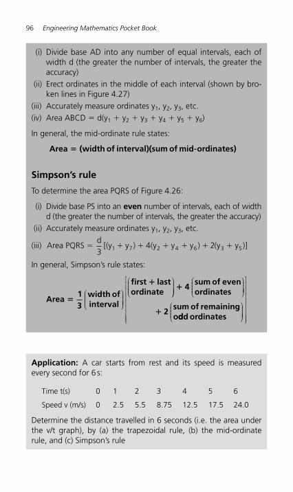
96 Engineering Mathematics Pocket Book
(i) Divide base AD into any number of equal intervals, each of width d (the greater the number of intervals, the greater the accuracy)
(ii) Erect ordinates in the middle of each interval (shown by bro-ken lines in Figure 4.27 )
(iii) Accurately measure ordinates y 1 , y 2 , y 3 , etc. (iv) Area ABCD � d(y 1 � y 2 � y 3 � y 4 � y 5 � y 6 )
In general, the mid-ordinate rule states:
Area (width of interval)(sum of mid-ordinates)�
Simpson’s rule
To determine the area PQRS of Figure 4.26 :
(i) Divide base PS into an even number of intervals, each of width d (the greater the number of intervals, the greater the accuracy)
(ii) Accurately measure ordinates y 1 , y 2 , y 3 , etc.
(iii) Area PQRS
d[(y y ) (y y y ) (y y )]� � � � � � �
34 21 7 2 4 6 3 5
In general, Simpson’s rule states:
Area13
width ofinterval
first lastordinate
�
�
⎛⎝⎜⎜⎜
⎞⎠⎟⎟⎟⎟
⎛⎝⎜⎜⎜
⎞⎠⎠⎟⎟⎟⎟
⎛⎝⎜⎜⎜
⎞⎠⎟⎟⎟⎟�
�
4sum of evenordinates
2sum of remainingoddd ordinates
⎛⎝⎜⎜⎜
⎞⎠⎟⎟⎟⎟
⎡
⎣
⎢⎢⎢⎢⎢⎢⎢
⎤
⎦
⎥⎥⎥⎥⎥⎥⎥
Application: A car starts from rest and its speed is measured every second for 6 s:
Time t(s) 0 1 2 3 4 5 6
Speed v (m/s) 0 2.5 5.5 8.75 12.5 17.5 24.0
Determine the distance travelled in 6 seconds (i.e. the area under the v/t graph), by (a) the trapezoidal rule, (b) the mid-ordinate rule, and (c) Simpson’s rule
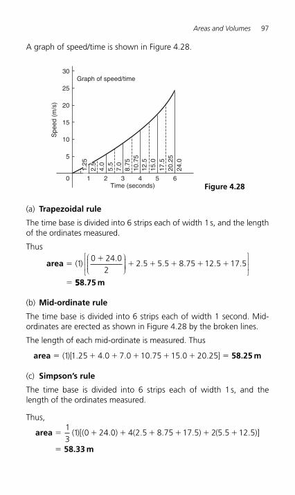
Areas and Volumes 97
A graph of speed/time is shown in Figure 4.28 .
30
25
Graph of speed/time
20
15
Spe
ed (
m/s
)
10
5
0 1 2 3 4 5 6Time (seconds)
4.0
7.0
15.0
5.5
8.75
10.7
512
.5
17.5
20.2
524
.0
2.5
1.25
Figure 4.28
(a) Trapezoidal rule
The time base is divided into 6 strips each of width 1 s, and the length of the ordinates measured.
Thus
area ��
� � � � �
�
( )10 24 0
22 5 5 5 8 75 12 5 17 5
.. . . . .
⎛⎝⎜⎜⎜
⎞⎠⎟⎟⎟⎟
⎡
⎣⎢⎢
⎤
⎦⎥⎥
558.75 m
(b) Mid-ordinate rule
The time base is divided into 6 strips each of width 1 second. Mid-ordinates are erected as shown in Figure 4.28 by the broken lines.
The length of each mid-ordinate is measured. Thus
area 58.25 m� � � � � � �( )[ ]1 1 25 4 0 7 0 10 75 15 0 20 25. . . . . .
(c) Simpson’s rule
The time base is divided into 6 strips each of width 1 s, and the length of the ordinates measured.
Thus,
area
58.33 m
� � � � � � �
�
13
1 0 24 0 4 2 5 8 75 17 5 2 5 5 12 5( )[( ) ( ) ( )]. . . . . .
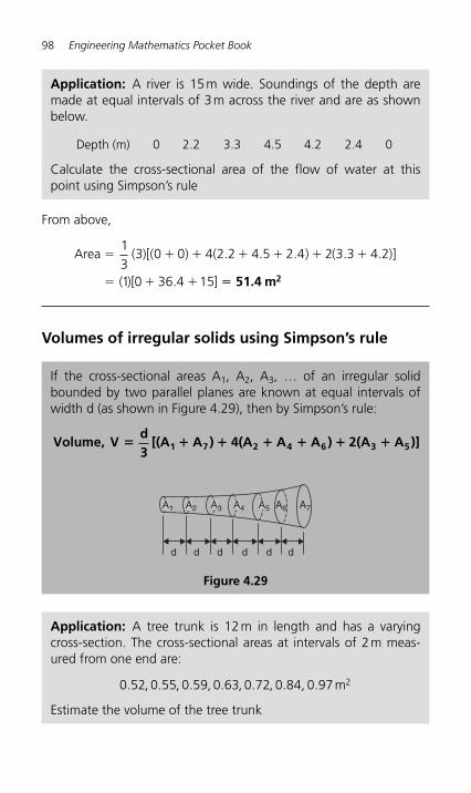
98 Engineering Mathematics Pocket Book
From above,
Area ( )[( ) ( ) ( )]
( )[ ]
� � � � � � �
� � �
13
3 0 0 4 2 2 4 5 2 4 2 3 3 4 2
1 0 36 4 15
. . . . .
. �� 51.4 m2
Volumes of irregular solids using Simpson’s rule
Application: A river is 15 m wide. Soundings of the depth are made at equal intervals of 3 m across the river and are as shown below.
Depth (m) 0 2.2 3.3 4.5 4.2 2.4 0
Calculate the cross-sectional area of the flow of water at this point using Simpson’s rule
If the cross-sectional areas A 1, A 2, A 3, … of an irregular solid bounded by two parallel planes are known at equal intervals of width d (as shown in Figure 4.29 ), then by Simpson’s rule:
Volume, Vd3
[(A A ) 4(A A A ) 2(A A )]1 7 2 4 6 3 5� � � � � � �
A6 A7
d d d d d d
A5A4A3A2A1
Figure 4.29
Application: A tree trunk is 12 m in length and has a varying cross-section. The cross-sectional areas at intervals of 2 m meas-ured from one end are:
0 52 0 55 0 59 0 63 0 72 0 84 0 97 2. , . , . , . , . , . , . m Estimate the volume of the tree trunk
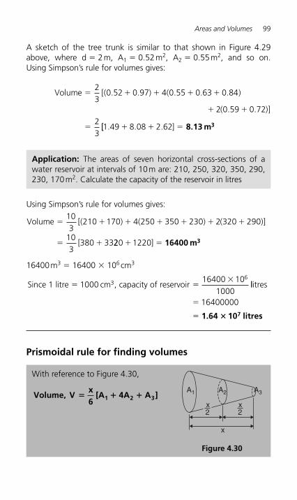
Areas and Volumes 99
A sketch of the tree trunk is similar to that shown in Figure 4.29 above, where d � 2 m, A 1 � 0.52 m 2, A 2 � 0.55 m 2, and so on. Using Simpson’s rule for volumes gives:
Volume [( ) ( )
( )]
� � � � �
� �
�
23
0 52 0 97 4 0 55 0 63 0 84
2 0 59 0 7223
. . . . .
. .
[[ ]1 49 8 08 2 62. . .� � � 8.13 m3
Application: The areas of seven horizontal cross-sections of a water reservoir at intervals of 10 m are: 210, 250, 320, 350, 290, 230, 170 m 2 . Calculate the capacity of the reservoir in litres
Using Simpson’s rule for volumes gives:
Volume [( ) ( ) ( )]
[
� � � � � � �
� �
103
210 170 4 250 350 230 2 320 290
103
380 33220 1220� �] 16400 m3
16400 m 3 � 16400 � 10 6 cm 3
Since 1 litre cm , capacity of reservoir3� ��
100016400 10
1000
6llitres
�
�
16400000
1.64 10 litres7�
Prismoidal rule for finding volumes
With reference to Figure 4.30 ,
Volume, Vx6
[A 4A A ]1 2 3� � �
2
A1 A2 A3
2x x
x
Figure 4.30
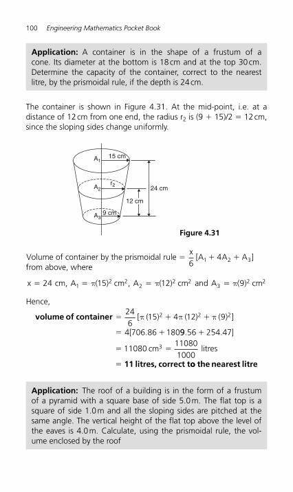
100 Engineering Mathematics Pocket Book
The container is shown in Figure 4.31 . At the mid-point, i.e. at a distance of 12 cm from one end, the radius r 2 is (9 � 15)/2 � 12 cm, since the sloping sides change uniformly.
15 cm
24 cm
9 cm
A1
A2r2
A3
12 cm
Figure 4.31
Application: A container is in the shape of a frustum of a cone. Its diameter at the bottom is 18 cm and at the top 30 cm. Determine the capacity of the container, correct to the nearest litre, by the prismoidal rule, if the depth is 24 cm.
Volume of container by the prismoidal rule
x[A A A ]� � �
641 2 3
from above, where
Application: The roof of a building is in the form of a frustum of a pyramid with a square base of side 5.0 m. The flat top is a square of side 1.0 m and all the sloping sides are pitched at the same angle. The vertical height of the flat top above the level of the eaves is 4.0 m. Calculate, using the prismoidal rule, the vol-ume enclosed by the roof
x cm, A ( ) cm , A ( ) cm and A ( ) cm� � � �24 15 12 912 2
22 2
32 2π π π
Hence,
volume of container � � �
� �
246
15 4 12 9
706 86 180
2 2 2[ ( ) ( ) ( ) ]
4[
π π π
. 99 56 254 47
11080110801000
3
. .�
� �
�
]
cm litres
11 litres, correct too the nearest litre
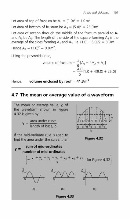
Areas and Volumes 101
Let area of top of frustum be A 1 � (1.0) 2 � 1.0 m 2
Let area of bottom of frustum be A 3 � (5.0) 2 � 25.0 m 2
Let area of section through the middle of the frustum parallel to A 1 and A 3 be A 2. The length of the side of the square forming A 2 is the average of the sides forming A 1 and A 3 , i.e. (1.0 � 5.0)/2 � 3.0 m.
Hence A 2 � (3.0) 2 � 9.0 m 2 .
Using the prismoidal rule,
volume of frustumx
[A A A ]� � �6
41 2 3
�� � �4 06
1 0 4 9 0 25 0.
. . .[ ( ) ]
Hence, volume enclosed by roof � 41.3 m 3
4.7 The mean or average value of a waveform
The mean or average value, y, of the waveform shown in Figure 4.32 is given by:
y �area under curvelength of base, b
If the mid-ordinate rule is used to find the area under the curve, then:
ysum of mid-ordinates
number of mid-ordinates�
y� 1 �� � � � � �y y y y y y
for Figure 2 3 4 5 6 7
74 32.
⎛⎝⎜⎜⎜
⎞⎠⎟⎟⎟⎟
y
d d d d d d db
y1 y2 y3 y4 y5 y6 y7
Figure 4.32
Figure 4.33
(a)
0
Vm
V
t
(b)
0 t
Vm
V
0 t
Vm
V
(c)
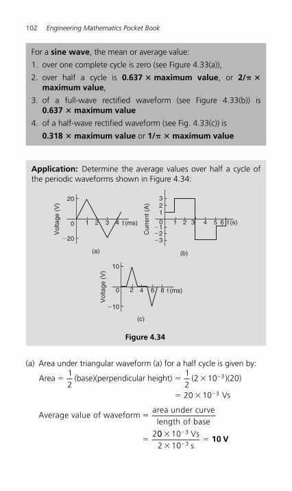
102 Engineering Mathematics Pocket Book
(a) Area under triangular waveform (a) for a half cycle is given by:
Area (base)(perpendicular height) ( )( )� � �
� �
�
�
12
12
2 10 20
20 10
3
3 Vs
Average value of waveformarea under curvelength of base
�
�200 10
2 10
3
3
�
��
�
�
Vss
10 V
For a sine wave , the mean or average value:
1. over one complete cycle is zero (see Figure 4.33(a) ),
2. over half a cycle is 0.637 � maximum value, or 2/π � maximum value ,
3. of a full-wave rectified waveform (see Figure 4.33(b) ) is 0.637 � maximum value
4. of a half-wave rectified waveform (see Fig. 4.33(c) ) is
0.318 � maximum value or 1/ π � maximum value
Application: Determine the average values over half a cycle of the periodic waveforms shown in Figure 4.34 :
(a)
(c)
(b)
20
0 21 3 4
Vol
tage
(V
)
�20
t (ms)
32
Cur
rent
(A
)
1
0 21 3 4 5 6�1�2�3
t (s)
Vol
tage
(V
)
10
�10
0 42 6 8 t (ms)
Figure 4.34
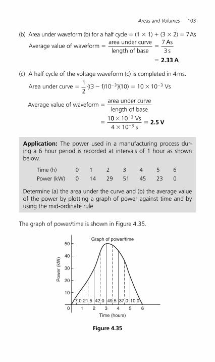
Areas and Volumes 103
(b) Area under waveform (b) for a half cycle � (1 � 1) � (3 � 2) � 7 As
Average value of waveformarea under curvelength of base
� �7 AAs
s3
� 2.33 A
(c) A half cycle of the voltage waveform (c) is completed in 4 ms.
Area under curve {( ) }( ) Vs� � � �� �1
23 110 10 10 103 3
Average value of waveformarea under curvelength of base
�
�100 10
4 10
3
3
�
��
�
�
Vss
2.5 V
Application: The power used in a manufacturing process dur-ing a 6 hour period is recorded at intervals of 1 hour as shown below.
Time (h) 0 1 2 3 4 5 6
Power (kW) 0 14 29 51 45 23 0
Determine (a) the area under the curve and (b) the average value of the power by plotting a graph of power against time and by using the mid-ordinate rule
The graph of power/time is shown in Figure 4.35 .
50
40
30
Pow
er (
kW)
20
10
0 21 3
Time (hours)
Graph of power/time
4 5 6
7.0 21.5 37.049.542.0 10.0
Figure 4.35
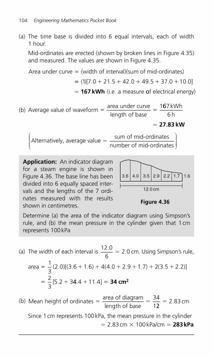
104 Engineering Mathematics Pocket Book
(a) The width of each interval is12 0
62 0
..� cm. Using Simpson’s rule,
area ( )[( ) ( ) ( )]
[
� � � � � � �
� �
13
2 0 3 6 1 6 4 4 0 2 9 1 7 2 3 5 2 2
23
5 2 3
. . . . . . . .
. 44 4 11 4. .� �] 34 cm2
(b) Mean height of ordinates
area of diagramlength of base
� �34122
2 83� . cm
Since 1 cm represents 100 kPa, the mean pressure in the cylinder � 2.83 cm � 100 kPa/cm � 283 kPa
(a) The time base is divided into 6 equal intervals, each of width 1 hour.
Mid-ordinates are erected (shown by broken lines in Figure 4.35 )and measured. The values are shown in Figure 4.35 .
Area under curve (width of interval)(sum of mid-ordinates)�
�� � � � � �
�
( )[ ]
(i.e. a measure
1 7 0 21 5 42 0 49 5 37 0 10 0. . . . . .
167 kWh oof electrical energy)
(b)
Average value of waveformarea under curvelength of base
� �1667
6kWhh
� 27.83 kW
Alternatively, average valuesum of mid-ordinates
number of�
mid-ordinates
⎛
⎝⎜⎜⎜⎜
⎞
⎠⎟⎟⎟⎟⎟
Application: An indicator diagramfor a steam engine is shown in Figure 4.36 . The base line has been divided into 6 equally spaced inter-vals and the lengths of the 7 ordi-nates measured with the results shown in centimetres.
Determine (a) the area of the indicator diagram using Simpson’s rule, and (b) the mean pressure in the cylinder given that 1 cm represents 100 kPa
3.6 3.5 2.9
12.0 cm
2.2 1.7 1.64.0
Figure 4.36
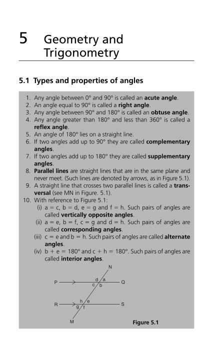
5 Geometry and Trigonometry
5.1 Types and properties of angles
1. Any angle between 0° and 90° is called an acute angle . 2. An angle equal to 90° is called a right angle .
3. Any angle between 90° and 180° is called an obtuse angle . 4. Any angle greater than 180° and less than 360° is called a
reflex angle. 5. An angle of 180° lies on a straight line. 6. If two angles add up to 90° they are called complementary
angles . 7. If two angles add up to 180° they are called supplementary
angles. 8. Parallel lines are straight lines that are in the same plane and
never meet. (Such lines are denoted by arrows, as in Figure 5.1 ). 9. A straight line that crosses two parallel lines is called a trans-
versal (see MN in Figure. 5.1 ). 10. With reference to Figure 5.1 :
(i) a � c, b � d, e � g and f � h. Such pairs of angles are called vertically opposite angles .
(ii) a � e, b � f, c � g and d � h. Such pairs of angles are called corresponding angles.
(iii) c � e and b � h. Such pairs of angles are called alternate angles .
(iv) b � e � 180° and c � h � 180°. Such pairs of angles are called interior angles.
P
R
Q
Sh e
g
M
N
f
d ac b
Figure 5.1
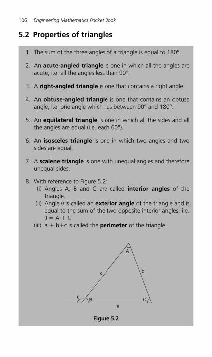
106 Engineering Mathematics Pocket Book
5.2 Properties of triangles
1. The sum of the three angles of a triangle is equal to 180°.
2. An acute-angled triangle is one in which all the angles are acute, i.e. all the angles less than 90°.
3. A right-angled triangle is one that contains a right angle.
4. An obtuse-angled triangle is one that contains an obtuse angle, i.e. one angle which lies between 90° and 180°.
5. An equilateral triangle is one in which all the sides and all the angles are equal (i.e. each 60°).
6. An isosceles triangle is one in which two angles and two sides are equal.
7. A scalene triangle is one with unequal angles and therefore unequal sides.
8. With reference to Figure 5.2 : (i) Angles A, B and C are called interior angles of the
t riangle. (ii) Angle θ is called an exterior angle of the triangle and is
equal to the sum of the two opposite interior angles, i.e. θ � A � C
(iii) a � b � c is called the perimeter of the triangle.
A
CBθ
bc
a
Figure 5.2
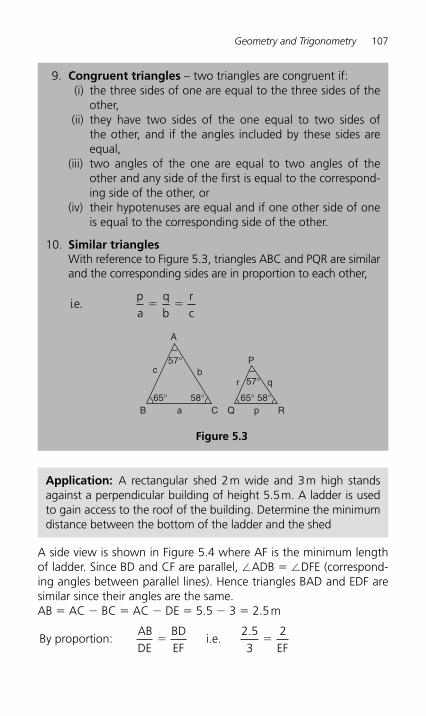
Geometry and Trigonometry 107
A side view is shown in Figure 5.4 where AF is the minimum length of ladder. Since BD and CF are parallel, � ADB � �DFE (correspond-ing angles between parallel lines). Hence triangles BAD and EDF are similar since their angles are the same.AB � AC � BC � AC � DE � 5.5 � 3 � 2.5 m
By proportion:
ABDE
BDEF
i.e.EF
� �2 53
2.
9. Congruent triangles – two triangles are congruent if: (i) the three sides of one are equal to the three sides of the
other, (ii) they have two sides of the one equal to two sides of
the other, and if the angles included by these sides are equal,
(iii) two angles of the one are equal to two angles of the other and any side of the first is equal to the correspond-ing side of the other, or
(iv) their hypotenuses are equal and if one other side of one is equal to the corresponding side of the other.
10. Similar triangles With reference to Figure 5.3 , triangles ABC and PQR are similar and the corresponding sides are in proportion to each other,
ie. . pa
qb
rc
� �
A
B Ca
cr
pQ R
P
q
65° 65° 58°58°
57°
57°b
Figure 5.3
Application: A rectangular shed 2 m wide and 3 m high stands against a perpendicular building of height 5.5 m. A ladder is used to gain access to the roof of the building. Determine the minimum distance between the bottom of the ladder and the shed
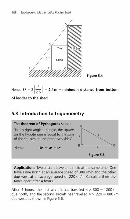
108 Engineering Mathematics Pocket Book
Hence EF � 2 3
2 5.
⎛⎝⎜⎜⎜
⎞⎠⎟⎟⎟⎟ � 2.4 m � minimum distance from bottom
of ladder to the shed
5.3 Introduction to trigonometry
A
B
C
D
EF
2 m
3 mShed
5.5m
Figure 5.4
The theorem of Pythagoras states:
‘In any right-angled triangle, the square on the hypotenuse is equal to the sum of the squares on the other two sides ’
Hence b a c2 2 2� �
A
c
a
b
B C
Figure 5.5
Application: Two aircraft leave an airfield at the same time. One travels due north at an average speed of 300 km/h and the other due west at an average speed of 220 km/h. Calculate their dis-tance apart after 4 hours
After 4 hours, the first aircraft has travelled 4 � 300 � 1200 km, due north, and the second aircraft has travelled 4 � 220 � 880 km due west, as shown in Figure 5.6 .
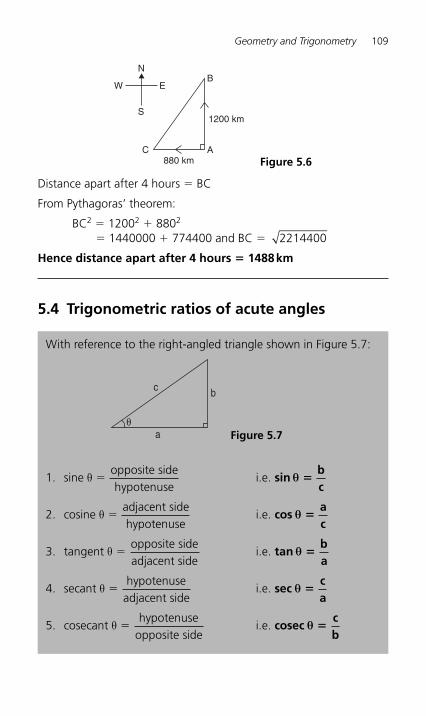
Geometry and Trigonometry 109
Distance apart after 4 hours � BC
From Pythagoras ’ theorem:
BC2 � 1200 2 � 880 2 � 1440000 � 774400 and BC � 2214400
Hence distance apart after 4 hours � 1488 km
5.4 Trigonometric ratios of acute angles
N
S
W EB
C A
1200 km
880 km Figure 5.6
With reference to the right-angled triangle shown in Figure 5.7 :
1. sine
opposite sidehypotenuse
i.e.θ � sin bc
θ �
2.
cosine
adjacent sidehypotenuse
i.e.θ � cos ac
θ �
3.
tangent
opposite sideadjacent side
i.e.θ � tan ba
θ �
4.
secant
hypotenuseadjacent side
i.e.θ � sec ca
θ �
5.
cosecant
hypotenuseopposite side
i.e.θ � cosec cb
θ �
θ
c
a
b
Figure 5.7
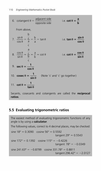
110 Engineering Mathematics Pocket Book
5.5 Evaluating trigonometric ratios
6.
cotangent i.e. θ �
adjacent sideopposite side
cot ab
θ �
From above,
7.
sincos
tanθθ
θ� � �
bcac
ba
i.e. tan θθθ
�sincos
8.
cossin
θθ
θ� � �
acbc
ab
cot i.e. cot cossin
θθθ
�
9.
sec θ
θ�
1cos
10. cosec θ
θ�
1sin
( )Note ’s’ and ’c’ go together
11.
cot θ
θ�
1tan
Secants, cosecants and cotangents are called the reciprocal ratios.
The easiest method of evaluating trigonometric functions of any angle is by using a calculator.
The following values, correct to 4 decimal places, may be checked:
sine 18° � 0.3090 cosine 56° � 0.5592 tangent 29° � 0.5543
sine 172° � 0.1392 cosine 115° � � 0.4226 tangent 78° � � 0.0349
sine 241.63° � � 0.8799 cosine 331.78° � 0.8811 tangent 296.42° � � 2.0127
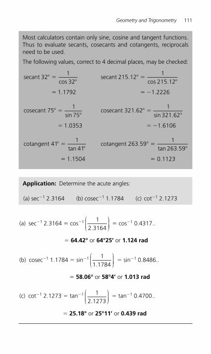
Geometry and Trigonometry 111
(a) sec � 1 2.3164 � cos � 1
12 3164.
⎛⎝⎜⎜⎜
⎞⎠⎟⎟⎟⎟ � cos � 1 0.4317..
� 64.42° or 64°25 ’ or 1.124 rad
(b) cosec � 1 1.1784 � sin � 1
11 1784.
⎛⎝⎜⎜⎜
⎞⎠⎟⎟⎟⎟
� sin � 1 0.8486..
� 58.06° or 58°4 ’ or 1.013 rad
(c) cot � 1 2.1273 � tan � 1
12 1273.
⎛⎝⎜⎜⎜
⎞⎠⎟⎟⎟⎟
� tan � 1 0.4700..
� 25.18° or 25°11 ’ or 0.439 rad
Most calculators contain only sine, cosine and tangent functions. Thus to evaluate secants, cosecants and cotangents, reciprocals need to be used.
The following values, correct to 4 decimal places, may be checked:
secant 3232
1.1792
� ��
�
1cos
secant 215.12215.12
1.2226
� ��
� �
1cos
cosecant 75175
� ��
�
sin
.1 0353
cosecant 321.62
1.6106
� ��
� �
1321 62sin .
cotangent 411
1
1.1504
� ��
�
tan 4
cotangent 263.591
0.1123
� ��
�
tan .263 59
Application: Determine the acute angles:
(a) sec � 1 2.3164 (b) cosec � 1 1.1784 (c) cot � 1 2.1273
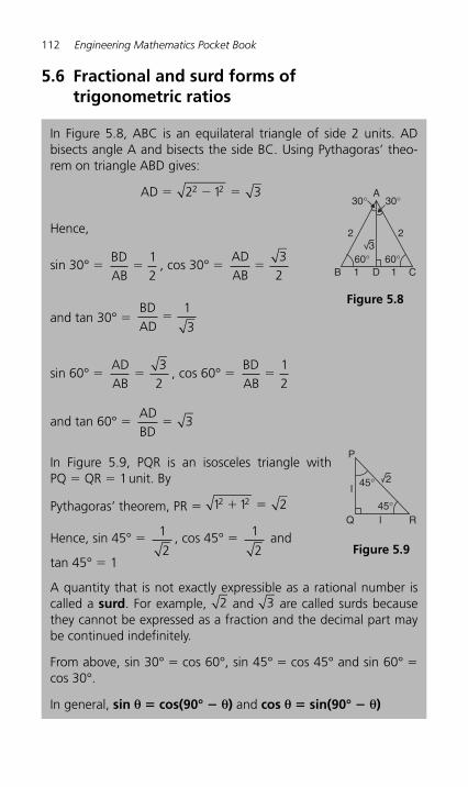
112 Engineering Mathematics Pocket Book
5.6 Fractional and surd forms of trigonometric ratios
In Figure 5.8 , ABC is an equilateral triangle of side 2 units. AD bisects angle A and bisects the side BC. Using Pythagoras ’ theo-rem on triangle ABD gives:
AD � � �2 1 32 2
Hence,
sin 30° �
BDAB
�12
, cos 30° �
ADAB
�3
2
and tan 30° � BDAD
�1
3
sin 60° �
ADAB
�3
2 , cos 60° �
BDAB
�12
and tan 60° � ADBD
� 3
In Figure 5.9 , PQR is an isosceles triangle with PQ � QR � 1 unit. By
Pythagoras ’ theorem, PR � 1 1 22 2� �
Hence, sin 45° �
1
2 , cos 45° �
1
2 and
tan 45° � 1
A quantity that is not exactly expressible as a rational number is called a surd. For example, 2 and 3 are called surds because they cannot be expressed as a fraction and the decimal part may be continued indefinitely.
From above, sin 30° � cos 60°, sin 45° � cos 45° and sin 60° � cos 30°.
In general, sin θ � cos(90° � θ ) and cos θ � sin(90° � θ )
A
2
B 1 D 1 C
23
30°30°
60° 60°
Figure 5.8
45°
45°
2
P
l
lQ R
Figure 5.9
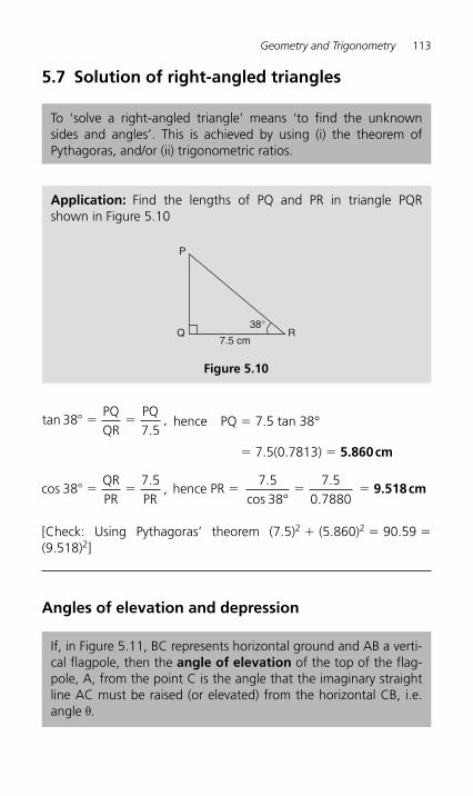
Geometry and Trigonometry 113
5.7 Solution of right-angled triangles
To ‘solve a right-angled triangle ’ means ‘to find the unknown sides and angles ’. This is achieved by using (i) the theorem of Pythagoras, and/or (ii) trigonometric ratios.
Application: Find the lengths of PQ and PR in triangle PQR shown in Figure 5.10
P
Q R38°
7.5 cm
Figure 5.10
tan
.,38
7 5� � �
PQQR
PQ
hence PQ � 7.5 tan 38°
� 7.5(0.7813) � 5.860 cm
cos
.,38
7 5� � �
QRPR PR
hence PR �
7 538
7 50 7880
.cos
..°
� � 9.518 cm
[Check: Using Pythagoras ’ theorem (7.5) 2 � (5.860) 2 � 90.59 � (9.518) 2 ]
Angles of elevation and depression
If, in Figure 5.11 , BC represents horizontal ground and AB a verti-cal flagpole, then the angle of elevation of the top of the flag-pole, A, from the point C is the angle that the imaginary straight line AC must be raised (or elevated) from the horizontal CB, i.e. angle θ .
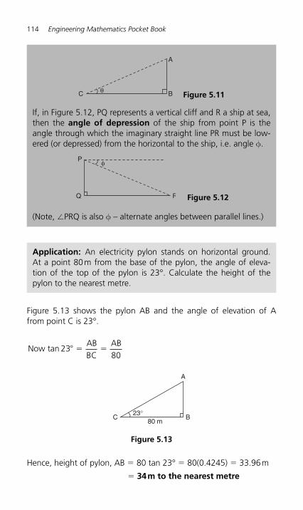
114 Engineering Mathematics Pocket Book
Figure 5.13 shows the pylon AB and the angle of elevation of A from point C is 23°.
Now tan 23
ABBC
AB� � �
80
If, in Figure 5.12 , PQ represents a vertical cliff and R a ship at sea, then the angle of depression of the ship from point P is the angle through which the imaginary straight line PR must be low-ered (or depressed) from the horizontal to the ship, i.e. angle φ .
(Note, � PRQ is also φ – alternate angles between parallel lines.)
P
Q R
φ
Figure 5.12
C B80 m
23°
A
Figure 5.13
C B
A
θ Figure 5.11
Application: An electricity pylon stands on horizontal ground. At a point 80 m from the base of the pylon, the angle of eleva-tion of the top of the pylon is 23°. Calculate the height of the pylon to the nearest metre.
Hence, height of pylon, AB � 80 tan 23° � 80(0.4245) � 33.96 m
� 34 m to the nearest metre
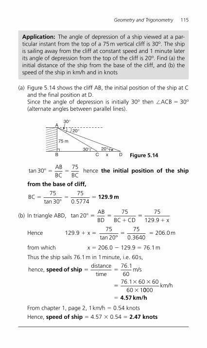
Geometry and Trigonometry 115
(a) Figure 5.14 shows the cliff AB, the initial position of the ship at C and the final position at D. Since the angle of depression is initially 30 o then � ACB � 30 o (alternate angles between parallel lines).
A
B C x D
75 m
30°
20°
30°
20° Figure 5.14
Application: The angle of depression of a ship viewed at a par-ticular instant from the top of a 75 m vertical cliff is 30 o. The ship is sailing away from the cliff at constant speed and 1 minute later its angle of depression from the top of the cliff is 20 o. Find (a) the initial distance of the ship from the base of the cliff, and (b) the speed of the ship in km/h and in knots
tan 30
75� � �
ABBC BC
hence the initial position of the ship
from the base of cliff,
BC �
�� �
7530
750 5774tan .
129.9 m
(b) In triangle ABD, tan
.20
75 75129 9
� � ��
��
ABBD BC CD x
Hence 129.9 � x �
7520
750 3640tan .°
� � 206.0 m
from which x � 206.0 � 129.9 � 76.1 m
Thus the ship sails 76.1 m in 1 minute, i.e. 60 s,
hence, distance
timem/sspeed of ship � �
�� �
�
76 160
76 1 60 6060 1
.
.0000
km/h
� 4.57 km/h From chapter 1, page 2, 1 km/h � 0.54 knots
Hence, speed of ship � 4.57 � 0.54 � 2.47 knots
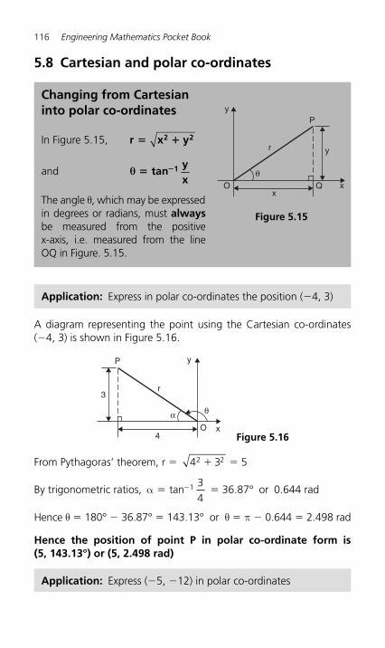
116 Engineering Mathematics Pocket Book
5.8 Cartesian and polar co-ordinates
Application: Express in polar co-ordinates the position ( � 4, 3)
Changing from Cartesian into polar co-ordinates
In Figure 5.15 , r x y2 2� �
and θ � �tanyx
1
The angle θ, which may be expressed in degrees or radians, must always be measured from the positive x-axis, i.e. measured from the line OQ in Figure. 5.15 .
O Q
P
r
y
y
xx
θ
Figure 5.15
O
P
r
y
x4
3
θα
Figure 5.16
A diagram representing the point using the Cartesian co-ordinates (�4, 3) is shown in Figure 5.16 .
From Pythagoras ’ theorem, r � 4 3 52 2� �
By trigonometric ratios, α � �tan 1 3
4 � 36.87° or 0.644 rad
Hence θ � 180° � 36.87° � 143.13° or θ � π � 0.644 � 2.498 rad
Hence the position of point P in polar co-ordinate form is (5, 143.13°) or (5, 2.498 rad)
Application: Express ( � 5, � 12) in polar co-ordinates
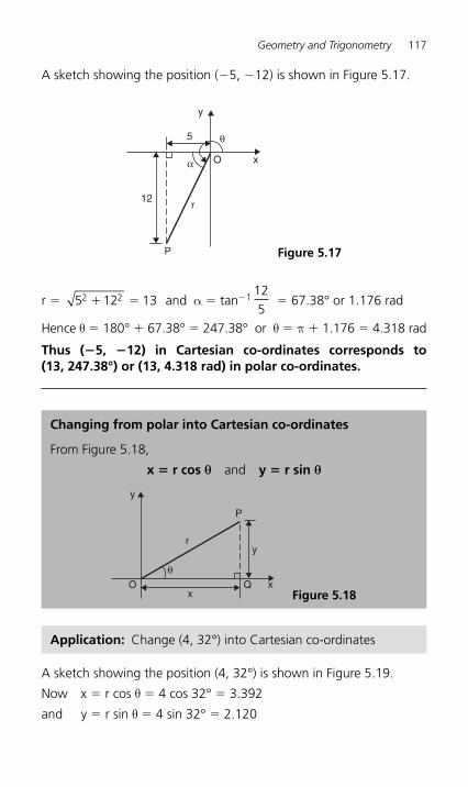
Geometry and Trigonometry 117
A sketch showing the position ( � 5, � 12) is shown in Figure 5.17 .
5
12
y
P
xO
r
α
θ
Figure 5.17
r � 5 12 132 2� � and α � tan � 1 125
� 67.38° or 1.176 rad
Hence θ � 180° � 67.38° � 247.38° or θ � π � 1.176 � 4.318 rad
Thus (�5, �12) in Cartesian co-ordinates corresponds to (13, 247.38°) or (13, 4.318 rad) in polar co-ordinates.
Changing from polar into Cartesian co-ordinates
From Figure 5.18 ,
x � r cos θ and y � r sin θ
O Q
P
r
y
y
xx
θ
Figure 5.18
Application: Change (4, 32°) into Cartesian co-ordinates
A sketch showing the position (4, 32°) is shown in Figure 5.19 .
Now x � r cos θ � 4 cos 32° � 3.392
and y � r sin θ � 4 sin 32° � 2.120
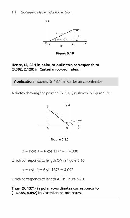
118 Engineering Mathematics Pocket Book
A sketch showing the position (6, 137°) is shown in Figure 5.20 .
Application: Express (6, 137°) in Cartesian co-ordinates
O
r � 4
y
y
xx
θ � 32°
Figure 5.19
Hence, (4, 32°) in polar co-ordinates corresponds to (3.392, 2.120) in Cartesian co-ordinates.
θ � 137°
y
O
r � 6
A x
B
Figure 5.20
x � r cos θ � 6 cos 137° � � 4.388
which corresponds to length OA in Figure 5.20 .
y � r sin θ � 6 sin 137° � 4.092
which corresponds to length AB in Figure 5.20 .
Thus, (6, 137°) in polar co-ordinates corresponds to (� 4.388, 4.092) in Cartesian co-ordinates.
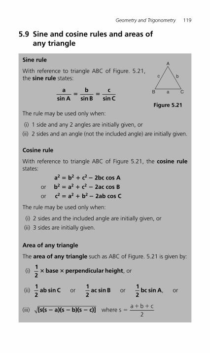
Geometry and Trigonometry 119
5.9 Sine and cosine rules and areas of any triangle
Sine rule
With reference to triangle ABC of Figure. 5.21 , the sine rule states:
asin A
bsin B
csin C
� �
The rule may be used only when:
(i) 1 side and any 2 angles are initially given, or
(ii) 2 sides and an angle (not the included angle) are initially given.
Cosine rule
With reference to triangle ABC of Figure 5.21 , the cosine rule states:
a2 � b 2 � c 2 � 2bc cos A
or b2 � a 2 � c 2 � 2ac cos B
or c2 � a 2 � b 2 � 2ab cos C
The rule may be used only when:
(i) 2 sides and the included angle are initially given, or
(ii) 3 sides are initially given.
Area of any triangle
The area of any triangle such as ABC of Figure. 5.21 is given by:
(i)
12
base perpendicular height� � , or
(ii)
12
ab sin C12
ac sin B12
bc sin Aor or , or
(iii)
[s(s a)(s b)(s c)]� � � where s
a b c�
� �
2
A
B Ca
c b
Figure 5.21
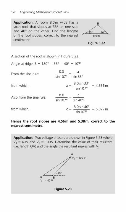
120 Engineering Mathematics Pocket Book
A section of the roof is shown in Figure 5.22 .
Angle at ridge, B � 180° � 33° � 40° � 107°
From the sine rule: 8 0107 33.
sinsina
��
�
from which, a �
8 0 33107
. sinsin
°°
� 4.556 m
Also from the sine rule: 8 0107 40.
sin sin°c
°�
from which, c �
8 0 40107
. sinsin
�
� � 5.377 m
Hence the roof slopes are 4.56 m and 5.38 m, correct to the nearest centimetre.
Application: A room 8.0 m wide has a span roof that slopes at 33 o on one side and 40 o on the other. Find the lengths of the roof slopes, correct to the nearest centimetre
A
B
C33° 40°8.0 m
Figure 5.22
Application: Two voltage phasors are shown in Figure 5.23 where V1 � 40 V and V 2 � 100 V. Determine the value of their resultant (i.e. length OA) and the angle the resultant makes with V 1
A
C B
V2 � 100 V
V1 � 40 V
45°
Figure 5.23
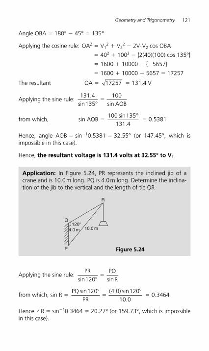
Geometry and Trigonometry 121
Angle OBA � 180° � 45° � 135°
Applying the cosine rule: OA 2 � V 1 2 � V22 � 2V 1 V 2 cos OBA
� 40 2 � 100 2 � { 2(40)(100) cos 135° }
� 1600 � 10000 � { � 5657 }
� 1600 � 10000 � 5657 � 17257
The resultant OA � 17257 � 131.4 V
Applying the sine rule: 131 4
135100.
sin sin° AOB�
from which, sin AOB �
100 135131 4sin
.°
� 0.5381
Hence, angle AOB � sin � 1 0.5381 � 32.55° (or 147.45°, which is impossible in this case).
Hence, the resultant voltage is 131.4 volts at 32.55° to V 1
Application: In Figure 5.24 , PR represents the inclined jib of a crane and is 10.0 m long. PQ is 4.0 m long. Determine the inclina-tion of the jib to the vertical and the length of tie QR
R
Q
10.0 m4.0 m120°
P Figure 5.24
Applying the sine rule: PR PO
Rsin sin120��
from which, sin R �
PQPR
sin ( . ) sin.
120 4 0 12010 0
��
� � 0.3464
Hence � R � sin � 1 0.3464 � 20.27° (or 159.73°, which is impossible in this case).
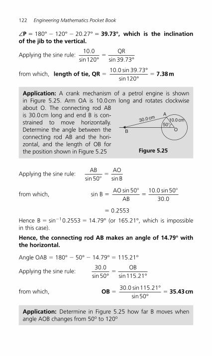
122 Engineering Mathematics Pocket Book
∠ P � 180° � 120° � 20.27° � 39.73°, which is the inclination of the jib to the vertical.
Applying the sine rule: 10 0
120 39 73.
sin sin .°QR
°�
from which, length of tie, QR �
10 0 39 73120
. sin .sin
°°
� 7.38 m
Application: A crank m echanism of a petrol engine is shown in Figure 5.25 . Arm OA is 10.0 cm long and rotates clockwise about O. The connecting rod AB is 30.0 cm long and end B is con-strained to move horizontally. Determine the angle between the connecting rod AB and the hori-zontal, and the length of OB for the position shown in Figure 5.25
B
A
O
10.0 cm50°
30.0 cm
Figure 5.25
Applying the sine rule: AB AO
sin sin50��
B
from which, sin B �
AOABsin . sin
.50 10 0 50
30 0�
��
� 0.2553
Hence B � sin � 1 0.2553 � 14.79° (or 165.21°, which is impossible in this case).
Hence, the connecting rod AB makes an angle of 14.79° with the horizontal .
Angle OAB � 180° � 50° � 14.79° � 115.21°
Applying the sine rule: 30 0
50 115 21.
sin sin .°OB
°�
from which, OB �
30 0 115 2150
. sin .sin
°°
� 35.43 cm
Application: Determine in Figure 5.25 how far B moves when angle AOB changes from 50 o to 120 o
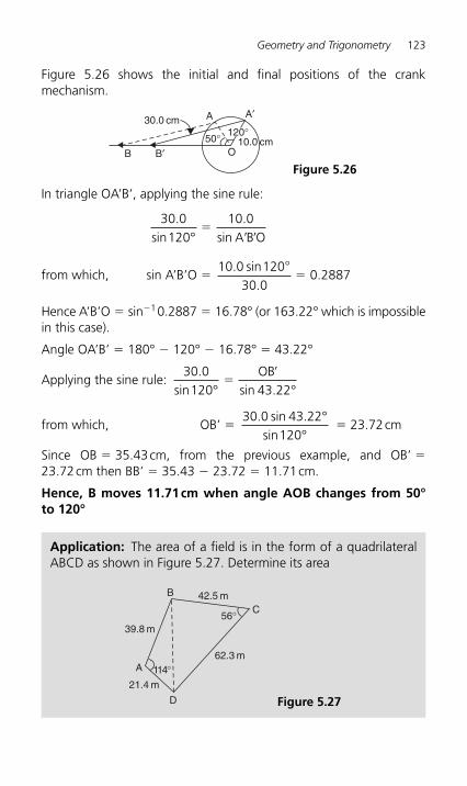
Geometry and Trigonometry 123
Figure 5.26 shows the initial and final positions of the crank mechanism.
50°OB′
A′
B
A
10.0 cm
30.0 cm120°
Figure 5.26
In triangle OA’B ’ , applying the sine rule:
30 0120
10 0.sin
.sin° A B O
�� �
from which, sin A’B’O �
10 0 12030 0
0 2887. sin
..
°�
Hence A’B’O � sin � 1 0.2887 � 16.78° (or 163.22° which is i mpossible in this case).
Angle OA’B ’ � 180° � 120° � 16.78° � 43.22°
Applying the sine rule: 30 0
120 43 22.
sin sin .°OB
°�
�
from which, OB ’ � 30 0 43 22
120. sin .sin
°°
� 23.72 cm
Since OB � 35.43 cm, from the previous example, and OB ’ � 23.72 cm then BB ’ � 35.43 � 23.72 � 11.71 cm.
Hence, B moves 11.71 cm when angle AOB changes from 50° to 120°
Application: The area of a field is in the form of a quadrilateral ABCD as shown in Figure 5.27 . Determine its area
B
C
D
A
56°
62.3 m
39.8 m
21.4 m
42.5 m
114°
Figure 5.27
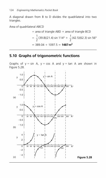
124 Engineering Mathematics Pocket Book
A diagonal drawn from B to D divides the quadrilateral into two triangles.
Area of quadrilateral ABCD
� area of triangle ABD � area of triangle BCD
�
12
(39.8)(21.4) sin 114° �
12
(42.5)(62.3) sin 56°
� 389.04 � 1097.5 � 1487 m 2
5.10 Graphs of trigonometric functions
Graphs of y � sin A, y � cos A and y � tan A are shown in Figure 5.28 .
1.0
�1.0
�4
�0.5
�1.0
�2
0.5
0.50 30 60 90 120 150 180 210 240 270 300 330 360
30 60 90 120 150 180 210 240 300 330 360
30 60 90 120150
180 210 240 270 300330
360
(a)
1.0
0.5
0
(b)
(c)
4
2
0 A°
A°
A°
y � tan A
y � cos A
y � sin A
270
y
y
y
Figure 5.28
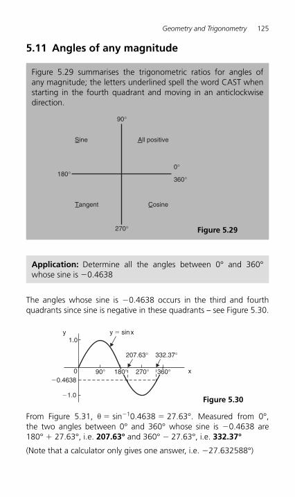
Geometry and Trigonometry 125
The angles whose sine is �0.4638 occurs in the third and fourth quadrants since sine is negative in these quadrants – see Figure 5.30 .
Figure 5.29 summarises the trigonometric ratios for angles of any magnitude; the letters underlined spell the word CAST when starting in the fourth quadrant and moving in an anticlockwise direction.
5.11 Angles of any magnitude
90°
180°
270°
360°
0°
Sine All positive
Tangent Cosine
Figure 5.29
Application: Determine all the angles between 0° and 360° whose sine is �0.4638
1.0
�1.0
�0.46380 90° 270°
332.37°207.63°
y � sinx
180° 360°
y
x
Figure 5.30
From Figure 5.31 , θ � sin � 1 0.4638 � 27.63°. Measured from 0°, the two angles between 0° and 360° whose sine is �0.4638 are 180° � 27.63°, i.e. 207.63° and 360° � 27.63°, i.e. 332.37°
(Note that a calculator only gives one answer, i.e. �27.632588°)
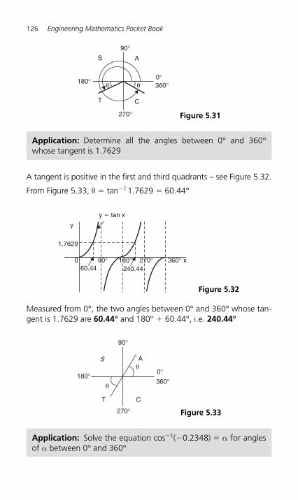
126 Engineering Mathematics Pocket Book
A tangent is positive in the first and third quadrants – see Figure 5.32 .
From Figure 5.33 , θ � tan � 1 1.7629 � 60.44°
90°
180°
270°
360°0°
θθ
A
C
S
T
Figure 5.31
180°
270°
360°
90°
0°
Sθ
θ
A
CT
Figure 5.33
1.7629
60.44 240.440 360°270°180°90°
y � tan x
y
x
Figure 5.32
Application: Determine all the angles between 0° and 360° whose tangent is 1.7629
Measured from 0°, the two angles between 0° and 360° whose tan-gent is 1.7629 are 60.44° and 180° � 60.44°, i.e. 240.44°
Application: Solve the equation cos � 1 ( � 0.2348) � α for angles of α between 0° and 360°
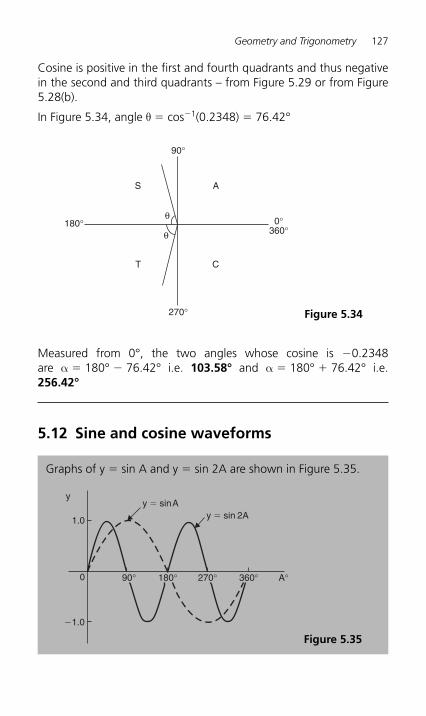
Geometry and Trigonometry 127
Cosine is positive in the first and fourth quadrants and thus negative in the second and third quadrants – from Figure 5.29 or from Figure 5.28 (b).
In Figure 5.34 , angle θ � cos � 1 (0.2348) � 76.42°
S
180°
90°
270°
0°360°
θ
θ
T
A
C
Figure 5.34
Measured from 0°, the two angles whose cosine is �0.2348are α � 180° � 76.42° i.e. 103.58° and α � 180° � 76.42° i.e. 256.42°
5.12 Sine and cosine waveforms
Graphs of y � sin A and y � sin 2 A are shown in Figure 5.35.
1.0
�1.0
0 A°
y � sin 2Ay � sinA
90° 180° 270° 360°
y
Figure 5.35
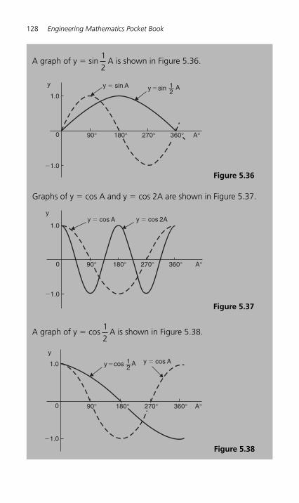
128 Engineering Mathematics Pocket Book
A graph of y � sin12
A is shown in Figure 5.36 .
Graphs of y � cos A and y � cos 2A are shown in Figure 5.37 .
A graph of y � cos 12
A is shown in Figure 5.38 .
1.0
�1.0
0
� sin 12
y � sin A
270°90° A°360°180°
yy A
Figure 5.36
1.0
�1.0
0
y � cos A y � cos 2A
360°180° A°90° 270°
y
Figure 5.37
1.0
�1.0
0
� cos 12
y � cos A
360° A°90° 180° 270°
y
Ay
Figure 5.38
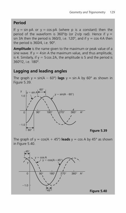
Geometry and Trigonometry 129
Period
If y � sin pA or y � cos pA (where p is a constant) then the period of the waveform is 360 o/p (or 2 π/p rad). Hence if y � sin 3 A then the period is 360/3, i.e. 120 o, and if y � cos 4 A then the period is 360/4, i.e. 90 o .
Amplitude is the name given to the maximum or peak value of a sine wave. If y � 4 sin A the maximum value, and thus amplitude, is 4. Similarly, if y � 5 cos 2A, the amplitude is 5 and the period is 360o /2, i.e. 180 o .
Lagging and leading angles
The graph y � sin(A � 60°) lags y � sin A by 60° as shown in Figure 5.39.
The graph of y � cos(A � 45°) leads y � cos A by 45° as shown in Figure 5.40.
1.0
60°
�1.0
0
y � sin Ay � sin(A�60°)
270°90°
60°
A°180° 360°
y
Figure 5.39
�1.0
45°
45°
0
y � cos Ay � cos(A�45°)
360°180° A°90° 270°
y
Figure 5.40
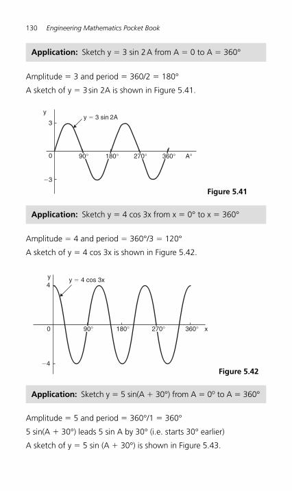
130 Engineering Mathematics Pocket Book
Amplitude � 3 and period � 360/2 � 180°
A sketch of y � 3 sin 2A is shown in Figure 5.41 .
y � 4 cos 3x
0
�4
4
180° 360° x90° 270°
y
Figure 5.42
3
�3
0
y � 3 sin 2A
A°360°270°180°90°
y
Figure 5.41
Application: Sketch y � 3 sin 2 A from A � 0 to A � 360°
Amplitude � 4 and period � 360°/3 � 120°
A sketch of y � 4 cos 3x is shown in Figure 5.42 .
Application: Sketch y � 4 cos 3x from x � 0° to x � 360°
Application: Sketch y � 5 sin(A � 30°) from A � 0o to A � 360°
Amplitude � 5 and period � 360°/1 � 360°
5 sin(A � 30°) leads 5 sin A by 30° (i.e. starts 30° earlier)
A sketch of y � 5 sin (A � 30°) is shown in Figure 5.43 .
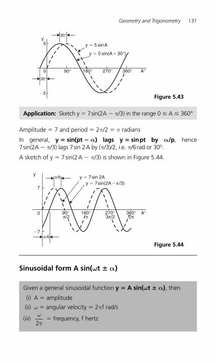
Geometry and Trigonometry 131
Amplitude � 7 and period � 2 π /2 � π radians
In general, y � sin(pt � α) lags y � sin pt by α/p, hence 7 sin(2A � π/3) lags 7 sin 2 A by ( π/3)/2, i.e. π/6 rad or 30 o .
A sketch of y � 7 sin(2 A � π /3) is shown in Figure 5.44 .
5
�5
0
y � 5 sinA
y � 5 sin(A�30°)
270°90°
30°
30°
A°180° 360°
y
Figure 5.43
Application: Sketch y � 7 sin(2A � π/3) in the range 0 � A � 360°
0
7
�7
y � 7sin 2Ay
y � 7sin(2A�π /3)
360°270°180°90° A°
π /6
3π/2 2πππ/2
π/6
Figure 5.44
Sinusoidal form A sin( ω t � α )
Given a general sinusoidal function y � A sin( ω t � α ) , then
(i) A � amplitude
(ii) ω � angular velocity � 2 π f rad/s
(iii) ωπ2
� frequency, f hertz
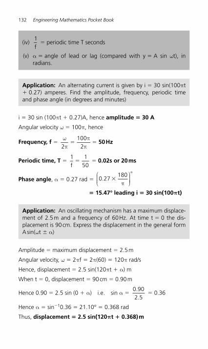
132 Engineering Mathematics Pocket Book
i � 30 sin (100 π t � 0.27)A, hence amplitude � 30 A
Angular velocity ω � 100 π , hence
Frequency, f � ωπ
ππ2
1002
� � 50 Hz
Periodic time, T � 1 1
50f� � 0.02s or 20 ms
Phase angle , α � 0.27 rad � 0 27180
. �π
⎛⎝⎜⎜⎜
⎞⎠⎟⎟⎟⎟�
� 15.47° leading i � 30 sin(100πt)
(iv) 1f
� periodic time T seconds
(v) α � angle of lead or lag (compared with y � A sin ωt), in radians.
Application: An alternating current is given by i � 30 sin(100 π t � 0.27) amperes. Find the amplitude, frequency, periodic time and phase angle (in degrees and minutes)
Application: An oscillating mechanism has a maximum displace-ment of 2.5 m and a frequency of 60 Hz. At time t � 0 the dis-placement is 90 cm. Express the displacement in the general form A sin( ω t α )
Amplitude � maximum displacement � 2.5 m
Angular velocity, ω � 2 π f � 2 π (60) � 120 π rad/s
Hence, displacement � 2.5 sin(120 π t � α ) m
When t � 0, displacement � 90 cm � 0.90 m
Hence 0.90 � 2.5 sin (0 � α) i.e. sin α � 0 902 5..
� 0.36
Hence α � sin � 1 0.36 � 21.10° � 0.368 rad
Thus, displacement � 2.5 sin(120 π t � 0.368) m
Geometry and Trigonometry 133
(a) Amplitude � 340 V
Angular velocity, ω � 50 π � 2 π f
Frequency, f � ωπ
ππ2
502
� � 25 Hz
Periodic time, T � 1 1
25f� � 0.04 s or 40 ms
Phase angle � 0.541 rad � 0 541180
. ��
π
⎛⎝⎜⎜⎜
⎞⎠⎟⎟⎟⎟
� 31� lagging v � 340 sin(50 π t)
(b) When t � 0, v � 340 sin(0 � 0.541) � 340 sin( �31°) � � 175.1 V
(c) When t � 10 ms then v � 340 sin(50 π � 10 � 10 � 3 � 0.541)
� 340 sin(1.0298) � 340 sin 59°
� 291.4 volts
(d) When v � 200 volts then 200 � 340 sin(50 π t � 0.541)
200340
� sin(50 π t � 0.541)
Hence (50 π t � 0.541) � sin � 1 200340
� 36.03° or 0.6288 rad
50 π t � 0.6288 � 0.541 � 1.1698
Hence when v � 200 V, time, t � 1 1698
50.
π � 7.447 ms
Application: The instantaneous value of voltage in an a.c. circuit at any time t seconds is given by v � 340 sin(50 π t � 0.541) volts. Determine
(a) the amplitude, frequency, periodic time and phase angle (in degrees),
(b) the value of the voltage when t � 0, (c) the value of the voltage when t � 10 ms, (d) the time when the voltage first reaches 200 V, and (e) the time when the voltage is a maximum
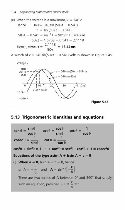
134 Engineering Mathematics Pocket Book
(e) When the voltage is a maximum, v � 340 V Hence 340 � 340 sin (50 π t � 0.541)
1 � sin (50 π t � 0.541) 50 π t � 0.541 � sin � 1 1 � 90° or 1.5708 rad
50 π t � 1.5708 � 0.541 � 2.1118
Hence, time, t � 2 1118
50.
π � 13.44 ms
A sketch of v � 340 sin(50 π t � 0.541) volts is shown in Figure 5.45 .
5.13 Trigonometric identities and equations
tansincos
cotcossin
seccos
cosecsin
cottan
θθθ
θθ
θθ
θθ
θ
� � �
� �
1
1 1
�
θθ cos2 θ � sin 2 θ � 1 1 � tan 2 θ � sec 2 θ cot 2 θ � 1 � cosec 2 θ
Equations of the type a sin 2 A � b sin A � c � 0
(i) When a � 0 , b sin A � c � 0, hence
sin A � � cb
and A � sin � 1 �cb
⎛⎝⎜⎜⎜
⎞⎠⎟⎟⎟⎟
There are two values of A between 0° and 360° that satisfy
such an equation, provided �1 � cb
� 1
Voltage v
340291.4
200
0
�175.1
�340
7.447 13.44
10 30 t(ms)
v � 340 sin(50πt�0.541)
v � 340 sin 50πt
20 40
Figure 5.45
Geometry and Trigonometry 135
5 sin θ � 3 � 0, from which sin θ � � 3/5 � � 0.6000
Hence, θ � sin � 1 ( �0.6000). Sine is negative in the third and fourth quadrants (see Figure 5.46 ). The acute angle sin � 1 (0.6000) � 36.87° (shown as α in Figure 5.46 (b)).
Hence θ � 180° � 36.87° i.e. 216.87° or θ � 360° – 36.87° i.e. 323.13°
(ii) When b � 0 , a sin 2 A � c � 0, hence
sin 2 A � � ca
, sin A � �ca
⎛⎝⎜⎜⎜
⎞⎠⎟⎟⎟⎟ and A � sin � 1 �
ca
⎛⎝⎜⎜⎜
⎞⎠⎟⎟⎟⎟
If either a or c is a negative number, then the value within the square root sign is positive. Since when a square root is taken there is a positive and negative answer there are four values of A between 0° and 360° which satisfy such an equa-tion, provided �1 �
ca � 1
(iii) When a, b and c are all non-zero: a sin 2 A � b sin A � c � 0 is a quadratic equation in which the unknown is sin A. The solution of a quadratic equation is obtained either by factorising (if possible) or by using the quadratic formula:
sin Ab b 4ac
2a
2�
� � �( )
(iv) Often the trigonometric identities cos 2 A � sin 2 A � 1, 1 � tan 2 A � sec 2 A and cot 2 A � 1 � cosec 2 A need to be used to reduce equations to one of the above forms.
Application: Solve the trigonometric equation 5 sin θ � 3 � 0 for values of θ from 0° to 360°
Application: Solve 4 sec t � 5 for values of t between 0° and 360°
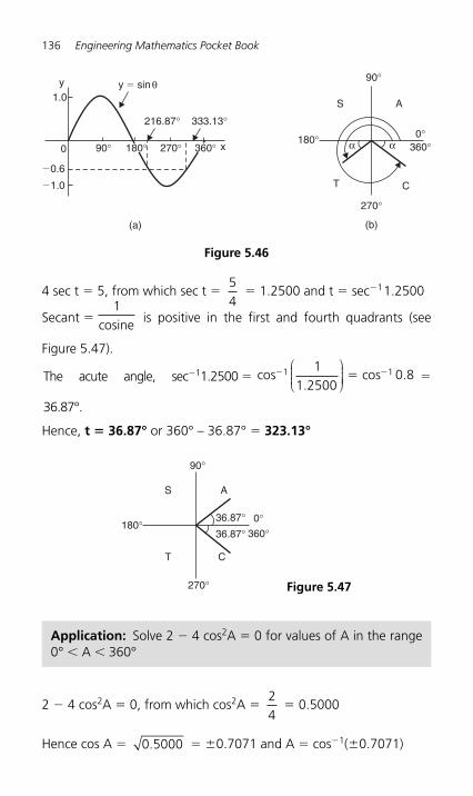
136 Engineering Mathematics Pocket Book
4 sec t � 5, from which sec t � 54
� 1.2500 and t � sec � 1 1.2500
Secant � 1
cosine is positive in the first and fourth quadrants (see
Figure 5.47 ).
The acute angle, sec � 11.2500 � cos cos� ��1 111 2500
0 8.
.⎛⎝⎜⎜⎜
⎞⎠⎟⎟⎟⎟ �
36.87°.
Hence, t � 36.87° or 360° – 36.87° � 323.13°
1.0
�1.0
�0.6
0 90° 270°
333.13°216.87°
y � sin θ
360°180°
(a)
y
x
Figure 5.46
90°
270°
(b)
CT
S A
360°180° 0°
α α
90°
AS
T C
180°0°
360°
270°
36.87°36.87°
Figure 5.47
Application: Solve 2 � 4 cos 2 A � 0 for values of A in the range 0° A 360°
2 � 4 cos 2 A � 0, from which cos 2 A � 24
� 0.5000
Hence cos A � 0 5000. � 0.7071 and A � cos � 1 ( 0.7071)
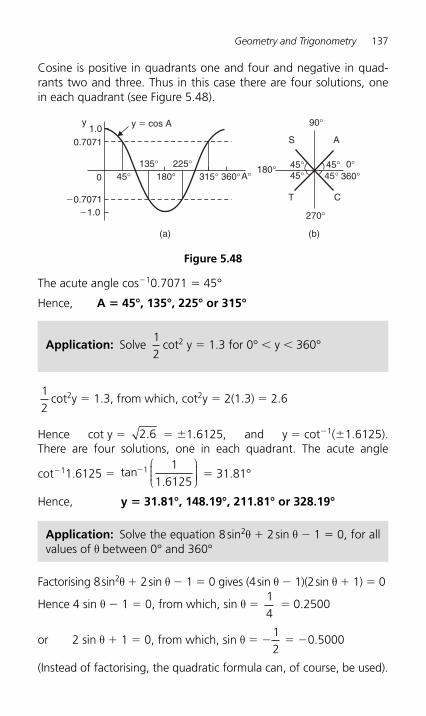
Geometry and Trigonometry 137
Cosine is positive in quadrants one and four and negative in quad-rants two and three. Thus in this case there are four solutions, one in each quadrant (see Figure 5.48 ).
1.00.7071
�0.7071�1.0
0 45° 315° 360°225°135°
y � cos A
180°
90°
S A
T C
270°
(b)(a)
360°180° 0°45°45°
45° 45°A°
y
Figure 5.48
The acute angle cos � 1 0.7071 � 45°
Hence, A � 45°, 135°, 225° or 315°
Application: Solve 12
cot 2 y � 1.3 for 0° y 360°
12
cot 2 y � 1.3, from which, cot 2 y � 2(1.3) � 2.6
Hence cot y � 2 6. � 1.6125, and y � cot � 1 ( 1.6125). There are four solutions, one in each quadrant. The acute angle
cot � 1 1.6125 � tan�1 11 6125.
⎛⎝⎜⎜⎜
⎞⎠⎟⎟⎟⎟ � 31.81°
Hence, y � 31.81°, 148.19°, 211.81° or 328.19°
Application: Solve the equation 8 sin 2 θ � 2 sin θ � 1 � 0, for all values of θ between 0° and 360°
Factorising 8 sin 2 θ � 2 sin θ � 1 � 0 gives (4 sin θ � 1)(2 sin θ � 1) � 0
Hence 4 sin θ � 1 � 0, from which, sin θ � 14
� 0.2500
or 2 sin θ � 1 � 0, from which, sin θ � � 12
� � 0.5000
(Instead of factorising, the quadratic formula can, of course, be used).
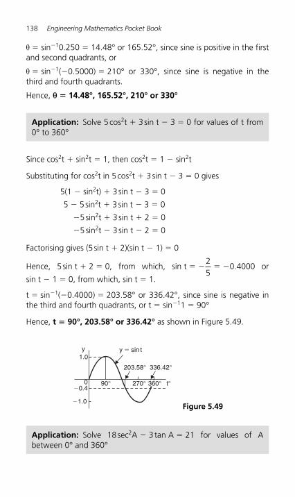
138 Engineering Mathematics Pocket Book
θ � sin � 1 0.250 � 14.48° or 165.52°, since sine is positive in the first and second quadrants, or
θ � sin � 1 ( � 0.5000) � 210° or 330°, since sine is negative in the third and fourth quadrants.
Hence, θ � 14.48°, 165.52°, 210° or 330°
Application: Solve 5 cos 2 t � 3 sin t � 3 � 0 for values of t from 0° to 360°
Since cos 2 t � sin 2 t � 1, then cos 2 t � 1 � sin 2 t
Substituting for cos 2 t in 5 cos 2 t � 3 sin t � 3 � 0 gives
5(1 � sin 2 t) � 3 sin t � 3 � 0
5 � 5 sin 2 t � 3 sin t � 3 � 0
� 5 sin 2 t � 3 sin t � 2 � 0
� 5 sin 2 t � 3 sin t � 2 � 0
Factorising gives (5 sin t � 2)(sin t � 1) � 0
Hence, 5 sin t � 2 � 0, from which, sin t � � 25
� � 0.4000 or
sin t � 1 � 0, from which, sin t � 1.
t � sin � 1 ( � 0.4000) � 203.58° or 336.42°, since sine is negative in the third and fourth quadrants, or t � sin � 1 1 � 90°
Hence, t � 90°, 203.58° or 336.42° as shown in Figure 5.49 .
1.0
�1.0
�0.40 90° 270°
336.42°203.58°
y � sin t
t°360°
y
Figure 5.49
Application: Solve 18 sec 2 A � 3 tan A � 21 for values of A between 0° and 360°
Geometry and Trigonometry 139
1 � tan 2 A � sec 2 A. Substituting for sec 2 A in18 sec 2 A � 3 tan A � 21 gives
18(1 � tan 2A) � 3 tan A � 21
i.e. 18 � 18 tan 2 A � 3 tan A � 21 � 0
18 tan 2 A � 3 tan A � 3 � 0
Factorising gives: (6 tan A � 3)(3 tan A � 1) � 0
Hence, 6 tan A � 3 � 0, from which, tan A � 36
� 0.5000
or 3 tan A � 1 � 0, from which, tan A � � 13
� � 0.3333
Thus, A � tan � 1 (0.5000) � 26.57° or 206.57°, since tangent is positive in the first and third quadrants, or A � tan � 1 ( � 0.3333) � 161.57° or 341.57°, since tangent is negative in the second and fourth quadrants. Hence, A � 26.57°, 161.57°, 206.57° or 341.57°
5.14 The relationship between trigonometric and hyperbolic functions
cos12
(e e )
sin12j
(e e )
j j
j j
θ
θ
θ θ
θ θ
� �
� �
�
�
cos j cosh
sin j j sinh
cosh j cos
sinh j j sin
tan j
θ θ
θ θ
θ θ
θ θ
θ
�
�
�
�
�
(1)
(2)
jj tanh
tanh j j tan
θ
θ θ�
Application: Verify that cos 2 j θ � sin 2 j θ � 1
140 Engineering Mathematics Pocket Book
From equation (3), cos j θ � cosh θ, and from equation (4), sin j θ � j sinh θ
Thus, cos 2 j θ � sin 2 j θ � cosh 2 θ � j 2 sinh 2 θ, and since j 2 � � 1 (from chapter 8),
cos 2 j θ � sin 2 j θ � cosh 2 θ � sinh 2 θ
But, cosh 2 θ � sinh 2 θ � 1, from page 38,
hence cos2 j θ � sin 2 j θ � 1
Application: Determine the corresponding hyperbolic identity by writing jA for θ in cot 2 θ � 1 � cosec 2 θ
Substituting jA for θ gives:
cot 2 jA � 1 � cosec 2jA, i.e. cossin sin
2
2 2
jAjA jA
� �11
But from equation (3), cos jA � cosh A
and from equation (4), sin jA � j sinh A
Hence cosh
sinh
2
2 2
Aj A � 1 �
12 2j Asinh
and since j 2 � � 1, � � � �coshsinh sinh
2
2 21
1AAA
Multiplying throughout by � 1, gives:
coshsinh sinh
2
2 21
1AA A
� � i.e. coth A 1 cosech A2 2� �
Application: Develop the hyperbolic identity corresponding to sin 3 θ � 3 sin θ � 4 sin 3 θ by writing jA for θ
Substituting jA for θ gives: sin 3jA � 3 sin jA � 4 sin 3 jA
and since from equation (4), sin jA � j sinh A,
j sinh 3A � 3j sinh A � 4j 3 sinh 3 A
Dividing throughout by j gives:
sinh 3A � 3 sinh A � j 24 sinh 3 A
But j 2 � � 1, hence sinh 3A � 3 sinh A � 4 sinh 3 A
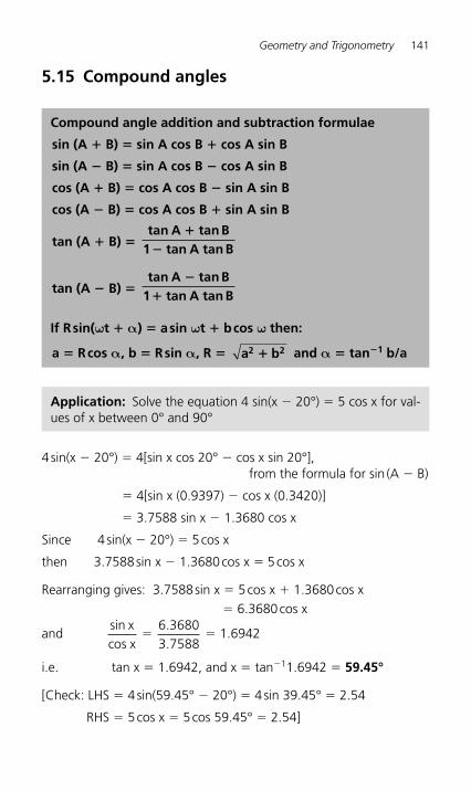
Geometry and Trigonometry 141
5.15 Compound angles
Compound angle addition and subtraction formulae
sin (A � B) � sin A cos B � cos A sin B
sin (A � B) � sin A cos B � cos A sin B
cos (A � B) � cos A cos B � sin A sin B
cos (A � B) � cos A cos B � sin A sin B
tan (A � B) � tan A tan B
1 tan A tan B�
�
tan (A � B) � tan A tan B
1 tan A tan B�
�
If R sin( ω t � α ) � a sin ω t � b cos ω then:
a � R cos α , b � R sin α , R � a b2 2� and α � tan � 1 b/a
Application: Solve the equation 4 sin(x � 20°) � 5 cos x for val-ues of x between 0° and 90°
4 sin(x � 20 ° ) � 4[sin x cos 20 ° � cos x sin 20°], from the formula for sin (A � B)
� 4[sin x (0.9397) � cos x (0.3420)]
� 3.7588 sin x � 1.3680 cos x
Since 4 sin(x � 20°) � 5 cos x
then 3.7588 sin x � 1.3680 cos x � 5 cos x
Rearranging gives: 3.7588 sin x � 5 cos x � 1.3680 cos x � 6.3680 cos x
and sincos
.
.xx
� 6 36803 7588
� 1.6942
i.e. tan x � 1.6942, and x � tan � 1 1.6942 � 59.45°
[Check: LHS � 4 sin(59.45° � 20°) � 4 sin 39.45° � 2.54
RHS � 5 cos x � 5 cos 59.45° � 2.54]
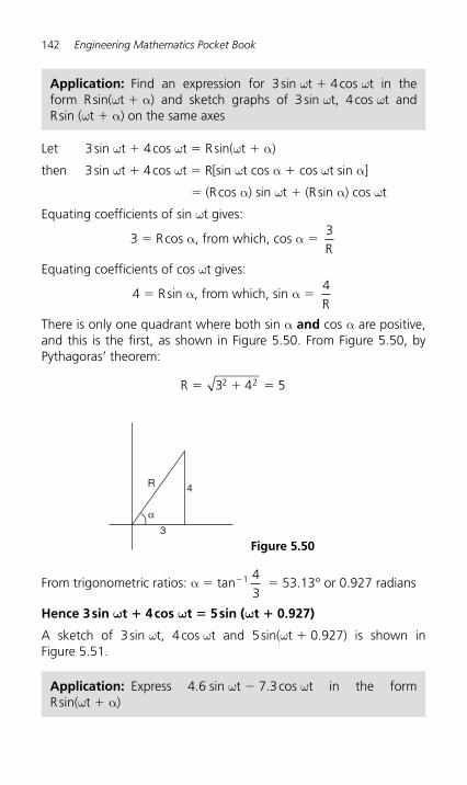
142 Engineering Mathematics Pocket Book
Let 3 sin ω t � 4 cos ω t � R sin( ω t � α )
then 3 sin ω t � 4 cos ω t � R[sin ω t cos α � cos ω t sin α ]
� (R cos α ) sin ω t � (R sin α ) cos ω t
Equating coefficients of sin ω t gives:
3 � R cos α , from which, cos α � 3R
Equating coefficients of cos ω t gives:
4 � R sin α , from which, sin α � 4R
There is only one quadrant where both sin α and cos α are positive, and this is the first, as shown in Figure 5.50 . From Figure 5.50 , by Pythagoras ’ theorem:
R � � �3 4 52 2
R 4
3
α
Figure 5.50
Application: Find an expression for 3 sin ω t � 4 cos ωt in the form R sin( ω t � α) and sketch graphs of 3 sin ωt, 4 cos ωt and R sin ( ω t � α ) on the same axes
From trigonometric ratios: α � tan � 1 43
� 53.13° or 0.927 radians
Hence 3 sin ω t � 4 cos ω t � 5 sin ( ω t � 0.927)
A sketch of 3 sin ωt, 4 cos ωt and 5 sin( ω t � 0.927) is shown in Figure 5.51 .
Application: Express 4.6 sin ω t � 7.3 cos ωt in the form R sin( ω t � α )
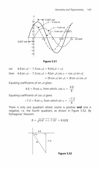
Geometry and Trigonometry 143
Let 4.6 sin ω t � 7.3 cos ω t � R sin( ω t � α )
then 4.6 sin ω t � 7.3 cos ω t � R [sin ω t cos α � cos ω t sin α ]
� (R cos α ) sin ω t � (R sin α ) cos ω t
Equating coefficients of sin ω t gives:
4.6 � R cos α , from which, cos α � 4 6.R
Equating coefficients of cos ω t gives:
�7.3 � R sin α , from which sin α � �7 3.
R
There is only one quadrant where cosine is positive and sine is negative, i.e. the fourth quadrant, as shown in Figure 5.52 . By Pythagoras ’ theorem:
R ( )� � � �4 6 7 3 8 6282 2. . .
4.6
R
α
�7.3
Figure 5.52
5
43
21
0�1
�20.927 rad
0.927 rady � 4 cos ωt
y � 3 sin ωt
y � 5 sin (ωt � 0.927)
ωt (rad)3π/2 2ππ
�3
�4
�5
π/2
y
Figure 5.51
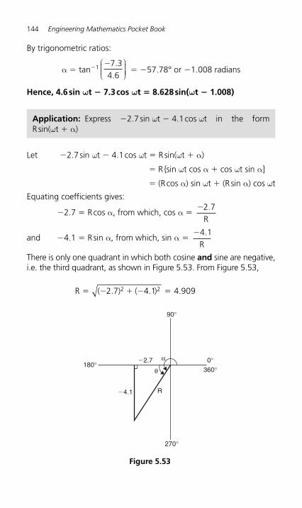
144 Engineering Mathematics Pocket Book
By trigonometric ratios:
α � tan � 1 �7 34 6
..
⎛⎝⎜⎜⎜
⎞⎠⎟⎟⎟⎟ � � 57.78° or � 1.008 radians
Hence, 4.6 sin ω t � 7.3 cos ω t � 8.628 sin( ω t � 1.008)
Application: Express �2.7 sin ω t � 4.1 cos ωt in the form R sin( ω t � α )
Let �2.7 sin ω t � 4.1 cos ω t � R sin( ω t � α )
� R { sin ω t cos α � cos ω t sin α ]
� (R cos α) sin ω t � (R sin α) cos ω t
Equating coefficients gives:
� 2.7 � R cos α , from which, cos α � �2 7.
R
and � 4.1 � R sin α , from which, sin α � �4 1.
R There is only one quadrant in which both cosine and sine are negative, i.e. the third quadrant, as shown in Figure 5.53 . From Figure 5.53 ,
R ( ) ( )2 2� � � � �2 7 4 1 4 909. . .
180°360°
90°
�2.7
�4.1 R
270°
α
θ0°
Figure 5.53
Geometry and Trigonometry 145
and θ � tan � 1 4 12 7
..
� 56.63°
Hence α � 180° � 56.63° � 236.63° or 4.130 radians
Thus, � 2.7 sin ω t � 4.1 cos ω t � 4.909 sin( ω t � 4.130)
An angle of 236.63° is the same as � 123.37° or � 2.153 radians
Hence, � 2.7 sin ω t � 4.1 cos ωt may also be expressed as 4.909 sin( ω t � 2.153) , which is preferred since it is the principalvalue (i.e. �π � α � π ).
Double angles
sin 2A � 2 sin A cos A
cos 2A � cos 2 A � sin 2 A � 1 � 2 sin 2 A � 2 cos 2 A � 1
tan 2A � 2 tan A
1 tan A2�
Application: I 3 sin 3 θ is the third harmonic of a waveform. Express the third harmonic in terms of the first harmonic sin θ , when I 3 � 1
When I 3 � 1, I 3 sin 3 θ � sin 3 θ � sin(2 θ � θ )
� sin 2 θ cos θ � cos 2 θ sin θ , from the sin(A � B) formula
� (2 sin θ cos θ ) cos θ � (1 � 2 sin 2 θ ) sin θ ,from the double angle expansions
� 2 sin θ cos 2 θ � sin θ � 2 sin 3 θ
� 2 sin θ (1 � sin 2 θ ) � sin θ � 2 sin 3 θ , (since cos2 θ � 1 � sin 2 θ )
� 2 sin θ � 2 sin 3 θ � sin θ � 2 sin 3 θ
i.e. sin 3 θ � 3 sin θ � 4 sin 3 θ
146 Engineering Mathematics Pocket Book
Changing products of sines and cosines into sums or differences
sin A cos B12
[sin (A B) sin (A B)]� � � � (3)
cos A sin B12
[sin (A B) sin (A B)]� � � � (4)
cos A cos B12
[cos (A B) cos (A B)]� � � � (5)
sin A sin B12
[cos (A B) cos (A B)]� � � � � (6)
Application: Express sin 4x cos 3x as a sum or difference of sines and cosines
From equation (3), sin 4x cos 3x � 12
[sin(4x � 3x) � sin(4x � 3x)]
� 12
(sin 7x � sin x)
Application: Express 2 cos 5 θ sin 2 θ as a sum or difference of sines or cosines
From equation (4),
2 cos 5 θ sin 2 θ � 2 12
5 2 5 2[sin( ) sin( )]θ θ θ θ� � �⎧⎨⎪⎪⎩⎪⎪
⎫⎬⎪⎪⎭⎪⎪
� sin 7 θ � sin 3 θ
Application: In an alternating current circuit, voltage v � 5 sin ω t and current i � 10 sin( ω t � π/6). Find an expression for the instantaneous power p at time t given that p � vi, expressing the answer as a sum or difference of sines and cosines
Geometry and Trigonometry 147
p � vi � (5 sin ωt)[10 sin ( ω t � π /6)] � 50 sin ω t sin( ω t � π /6)
From equation (6),
50 sin ω t sin( ω t � π /6) � (50) � � �
� �
12
66
{cos( )cos[ ( )]}
ω ω πω ω πt t
t t/
/−
� � 25 {cos( ) cos }2 6 6ω π πt � �/ /
i.e. instantaneous power, p � 25[cos π /6 � cos(2 ω t � π /6)]
Changing sums or differences of sines and cosines into products
sin X sin Y 2 sinX Y
2cos
X Y2
� �� �⎛
⎝⎜⎜⎜
⎞⎠⎟⎟⎟⎟
⎛⎝⎜⎜⎜
⎞⎠⎟⎟⎟⎟ (7)
sin X sin Y 2 cosX Y
2sin
X Y2
� �� �⎛
⎝⎜⎜⎜
⎞⎠⎟⎟⎟⎟
⎛⎝⎜⎜⎜
⎞⎠⎟⎟⎟⎟ (8)
cos X cos Y 2 cosX Y
2cos
X Y2
� �� �⎛
⎝⎜⎜⎜
⎞⎠⎟⎟⎟⎟
⎛⎝⎜⎜⎜
⎞⎠⎟⎟⎟⎟ (9)
cos X cos Y 2 sinX Y
2sin
X Y2
� � �� �⎛
⎝⎜⎜⎜
⎞⎠⎟⎟⎟⎟
⎛⎝⎜⎜⎜
⎞⎠⎟⎟⎟⎟ (10)
Application: Express sin 5 θ � sin 3 θ as a product
From equation (7),
sin 5 θ � sin 3 θ � 2 sin 5 3
25 3
2θ θ θ θ� �⎛
⎝⎜⎜⎜
⎞⎠⎟⎟⎟⎟
⎛⎝⎜⎜⎜
⎞⎠⎟⎟⎟⎟cos � 2 sin 4 θ cos θ
148 Engineering Mathematics Pocket Book
From equation (9),
sin 7x � sin x � 2 cos 7
27
2x x
sinx x� �⎛
⎝⎜⎜⎜
⎞⎠⎟⎟⎟⎟
⎛⎝⎜⎜⎜
⎞⎠⎟⎟⎟⎟ � 2 cos 4x sin 3x
Application: Express cos 2t � cos 5t as a product
From equation (10),
cos 2t � cos 5t � � 2 sin 2 5
22 5
2t t
sint t� �⎛
⎝⎜⎜⎜
⎞⎠⎟⎟⎟⎟
⎛⎝⎜⎜⎜
⎞⎠⎟⎟⎟⎟
� � 2 sin 72
32
t tsin �⎛⎝⎜⎜⎜
⎞⎠⎟⎟⎟⎟ � 2 sin
72
t sin 32
t
since sin t sin32
� � �32
⎛⎝⎜⎜⎜
⎞⎠⎟⎟⎟⎟
⎡
⎣⎢⎢
⎤
⎦⎥⎥t
Application: Express sin 7x � sin x as a product
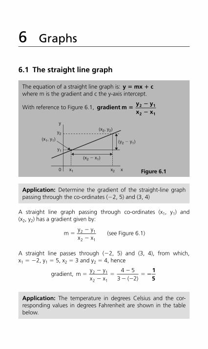
6 Graphs
6.1 The straight line graph
The equation of a straight line graph is: y � mx � cwhere m is the gradient and c the y-axis intercept.
With reference to Figure 6.1 , gradient my yx x
2 1
2 1
��
�
0
(x1, y1)
(x2, y2)
y1
y2
y
x
(x2 � x1)
x1 x2
(y2 � y1)
Figure 6.1
Application: Determine the gradient of the straight-line graph passing through the co-ordinates ( � 2, 5) and (3, 4)
A straight line graph passing through co-ordinates (x 1, y 1) and (x2 , y 2 ) has a gradient given by:
m
y yx x
��
�2 1
2 1 (see Figure 6.1 )
A straight line passes through ( �2, 5) and (3, 4), from which, x1 � � 2, y 1 � 5, x 2 � 3 and y 2 � 4, hence
gradient, my yx x ( )
��
��
�
� ��2 1
2 1
4 53 2
�15
Application: The temperature in degrees Celsius and the cor-responding values in degrees Fahrenheit are shown in the table below.
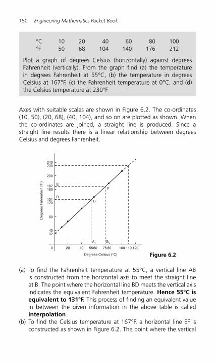
150 Engineering Mathematics Pocket Book
240230
200
Deg
rees
Fah
renh
eit (
°F)
160167
120
80
4032
0 20 40
A G
BD
EF
5560 75 80 100 120110
Degrees Celsius (°C)
131
Figure 6.2
Axes with suitable scales are shown in Figure 6.2 . The co-o rdinates (10, 50), (20, 68), (40, 104), and so on are plotted as shown. When the co-ordinates are joined, a straight line is produced. Since a straight line results there is a linear relationship between degrees Celsius and degrees Fahrenheit.
°C 10 20 40 60 80 100 °F 50 68 104 140 176 212
Plot a graph of degrees Celsius (horizontally) against degrees Fahrenheit (vertically). From the graph find (a) the temperature in degrees Fahrenheit at 55°C, (b) the temperature in degrees Celsius at 167°F, (c) the Fahrenheit temperature at 0°C, and (d) the Celsius temperature at 230°F
(a) To find the Fahrenheit temperature at 55°C, a vertical line AB is constructed from the horizontal axis to meet the straight line at B. The point where the horizontal line BD meets the vertical axis indicates the equivalent Fahrenheit temperature. Hence 55°C is equivalent to 131°F. This process of finding an equivalent value in between the given information in the above table is called interpolation .
(b) To find the Celsius temperature at 167°F, a horizontal line EF is constructed as shown in Figure 6.2 . The point where the vertical
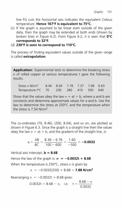
Graphs 151
line FG cuts the horizontal axis indicates the equivalent Celsius temperature. Hence 167°F is equivalent to 75°C.
(c) If the graph is assumed to be linear even outside of the given data, then the graph may be extended at both ends (shown by broken lines in Figure 6.2 ). From Figure 6.2 , it is seen that 0°Ccorresponds to 32°F.
(d) 230°F is seen to correspond to 110°C.
The process of finding equivalent values outside of the given range is called extrapolation .
Application: Experimental tests to determine the breaking stress σ of rolled copper at various temperatures t gave the following results.
Stress σ N/cm 2 8.46 8.04 7.78 7.37 7.08 6.63 Temperature t°C 70 200 280 410 500 640
Show that the values obey the law σ � at � b, where a and b are constants and determine approximate values for a and b. Use the law to determine the stress at 250°C and the temperature when the stress is 7.54 N/cm 2
The co-ordinates (70, 8.46), (200, 8.04), and so on, are plotted as shown in Figure 6.3 . Since the graph is a straight line then the values obey the law σ � at � b, and the gradient of the straight line, is:
aABBC
� ��
��
��
8 36 6 76100 600
1 60500
. . .�0.0032
Vertical axis intercept, b � 8.68
Hence the law of the graph is: σ � � 0.0032t � 8.68
When the temperature is 250°C, stress σ is given by
σ � � 0.0032(250) � 8.68 � 7.88 N/cm 2
Rearranging σ � � 0.0032t � 8.68 gives:
0.0032t � 8.68 � σ, i.e. t ��8 68
0 0032..
σ
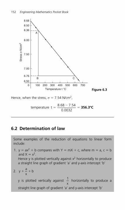
152 Engineering Mathematics Pocket Book
Hence, when the stress, σ � 7.54 N/cm 2 ,
temperature t ��
�8 68 7 54
0 0032. .
.356.3 C�
6.2 Determination of law
Some examples of the reduction of equations to linear form include:
1. y � ax 2 � b compares with Y � mX � c, where m � a, c � b and X � x 2 . Hence y is plotted vertically against x 2 horizontally to produce a straight line graph of gradient ‘ a ’ and y-axis intercept ‘ b ’
2. y
ax
b� �
y is plotted vertically against 1x
horizontally to produce a
straight line graph of gradient ‘ a ’ and y-axis intercept ‘ b ’
8.68
8.50
8.36
8.00
Str
ess
σ N
/cm
2
7.50
7.00
6.76
6.50
0 100 200 300 400Temperature t °C
500 600 700
A
B C
Figure 6.3
Graphs 153
Comparing Lad
b� � i.e. L a
db� �
1⎛⎝⎜⎜⎜
⎞⎠⎟⎟⎟⎟ with Y � mX � c shows
that L is to be plotted vertically against 1d
horizontally. Another table
of values is drawn up as shown below.
3. y � ax 2 � bx
Dividing both sides by x gives yx
ax b� �
Comparing with Y � mX � c shows that yx
is plotted verti-
cally against x horizontally to produce a straight line graph of
gradient ‘ a ’ and yx
axis intercept ‘ b ’ .
Determination of law involving logarithms
4. If y � ax n then lg y � lg(ax n ) � lg a � lg x n i.e. lg y � n lg x � lg a
5. If y � ab x then lg y � lg(ab x ) � lg a � lg b x � lg a � x lg b i.e. lg y � (lg b)x � lg a
6. If y � ae bx then ln y � ln(ae bx ) � ln a � ln(e bx ) � ln a � bxi.e. ln y � bx � ln a
Application: Values of load L newtons and distance d metres obtained experimentally are shown in the following table.
Load, L (N) 32.3 29.6 27.0 23.2 18.3 12.8 10.0 6.4
distance, d (m) 0.75 0.37 0.24 0.17 0.12 0.09 0.08 0.07
Verify that the load and distance are related by a law of the form
Lad
b� � and determine approximate values of a and b. Hence
calculate the load when the distance is 0.20 m and the distance when the load is 20 N
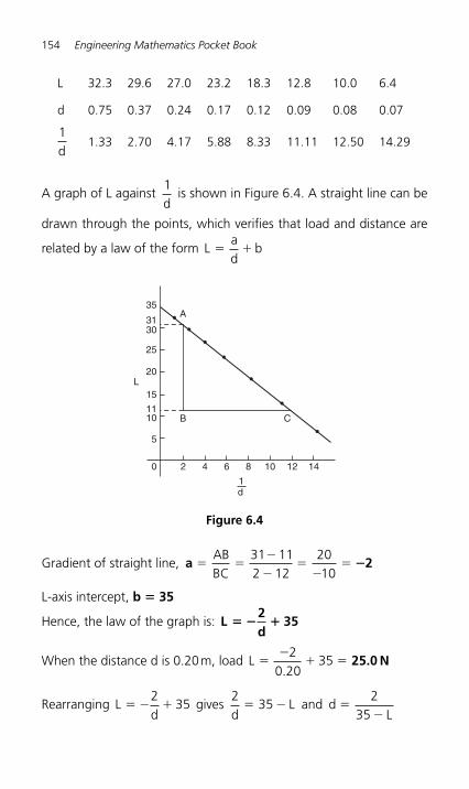
154 Engineering Mathematics Pocket Book
L 32.3 29.6 27.0 23.2 18.3 12.8 10.0 6.4
d 0.75 0.37 0.24 0.17 0.12 0.09 0.08 0.07
1d
1.33 2.70 4.17 5.88 8.33 11.11 12.50 14.29
A graph of L against 1d
is shown in Figure 6.4 . A straight line can be
drawn through the points, which verifies that load and distance are
related by a law of the form Lad
b� �
3031
35
25
20L
A
B C
15
5
0 2 4 6 8 10 12 14
1011
1d
Figure 6.4
Gradient of straight line, a 2� ��
��
��
ABBC
31 112 12
2010
�
L-axis intercept, b � 35
Hence, the law of the graph is: L2d
35� � �
When the distance d is 0.20 m, load L ��
� �2
0 2035
.25.0 N
Rearranging L2d
35� � � gives
2d
� �35 L and d ��
235 L
Graphs 155
Hence, when the load L is 20 N,
distance d ��
� �2
35 202
150.13 m
Application: The current flowing in, and the power dissipated by a resistor are measured experimentally for various values and the results are as shown below.
Current, I amperes 2.2 3.6 4.1 5.6 6.8
Power, P watts 116 311 403 753 1110
Show that the law relating current and power is of the form P � RI n , where R and n are constants, and determine the law
Taking logarithms to a base of 10 of both sides of P � RI n gives:
lg P � lg(RI n ) � lg R � lg I n � lg R � n lg I by the laws of logarithms
i.e. lg P � n lg I � lg R, which is of the form Y � mX � c,
showing that lg P is to be plotted vertically against lg I horizontally.
A table of values for lg I and lg P is drawn up as shown below.
I 2.2 3.6 4.1 5.6 6.8
lg I 0.342 0.556 0.613 0.748 0.833
P 116 311 403 753 1110
lg P 2.064 2.493 2.605 2.877 3.045
A graph of lg P against lg I is shown in Figure 6.5 and since a straight line results the law P � RI n is verified.
Gradient of straight line, nABBC
� ��
�� �
2 98 2 180 80 0 40
0 800 40
. .
. ...
2
It is not possible to determine the vertical axis intercept on sight since the horizontal axis scale does not start at zero. Selecting any point from the graph, say point D, where lg I � 0.70 and lg P � 2.78, and substituting values into
lg P � n lg I � lg R
gives: 2.78 � (2)(0.70) � lg R
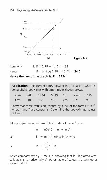
156 Engineering Mathematics Pocket Book
from which lg R � 2.78 � 1.40 � 1.38
Hence R � antilog 1.38 ( � 10 1.38 ) � 24.0
Hence the law of the graph is: P � 24.0 I 2
3.02.98
2.78
2.5
lgP
2.18
2.0
0.30 0.40 0.50 0.60
lg I
C B
A
D
0.800.70 0.90
Figure 6.5
Application: The current i mA flowing in a capacitor which is being discharged varies with time t ms as shown below.
i mA 203 61.14 22.49 6.13 2.49 0.615
t ms 100 160 210 275 320 390
Show that these results are related by a law of the form I � Ie t/T , where I and T are constants. Determine the approximate values of I and T.
Taking Napierian logarithms of both sides of i � Ie t/T gives
ln i � ln(Ie t/T ) � ln I � ln e t/T
i.e. ln i lntT
(since ln e x)x� � �I
or ln lni I� �1T
t⎛⎝⎜⎜⎜
⎞⎠⎟⎟⎟⎟
which compares with y � mx � c, showing that ln i is plotted verti-cally against t horizontally. Another table of values is drawn up as shown below.
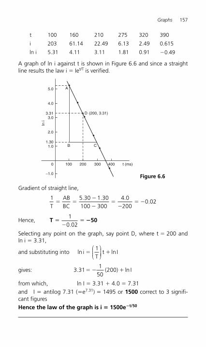
Graphs 157
t 100 160 210 275 320 390
i 203 61.14 22.49 6.13 2.49 0.615
ln i 5.31 4.11 3.11 1.81 0.91 � 0.49
A graph of ln i against t is shown in Figure 6.6 and since a straight line results the law i � Ie t/T is verified.
5.0 A
B C
D (200, 3.31)
4.0
3.31
ln i
3.0
2.0
1.301.0
0
−1.0
100 200 300 400 t (ms)
Figure 6.6
Gradient of straight line,
1 5 30 1 30100 300
4 0200
0 02T
ABBC
� ��
��
�� �
. . ..
Hence, T 50��
�1
0 02.�
Selecting any point on the graph, say point D, where t � 200 and ln i � 3.31,
and substituting into ln iT
t ln I� �1⎛
⎝⎜⎜⎜
⎞⎠⎟⎟⎟⎟
gives: 3 3150
200. ln� � �1
( ) I
from which, ln I � 3.31 � 4.0 � 7.31 and I � antilog 7.31 ( � e 7.31 ) � 1495 or 1500 correct to 3 signifi-cant figures Hence the law of the graph is i � 1500e � t/50
158 Engineering Mathematics Pocket Book
6.3 Logarithmic scales
Application: Experimental values of two related quantities x and y are shown below:
x 0.41 0.63 0.92 1.36 2.17 3.95
y 0.45 1.21 2.89 7.10 20.79 82.46
The law relating x and y is believed to be y � ax b, where a and b are constants.
Verify that this law is true and determine the approximate values of a and b
If y � ax b then lg y � b lg x � lg a, from page 153, which is of the form Y � mX � c, showing that to produce a straight line graph lg y is plotted vertically against lg x horizontally. x and y may be plotted directly on to log-log graph paper as shown in Figure 6.7 . The values of y range from 0.45 to 82.46 and 3 cycles are needed (i.e. 0.1 to 1, 1 to 10 and 10 to 100). The values of x range from 0.41 to 3.95 and 2 cycles are needed (i.e. 0.1 to 1 and 1 to 10). Hence ‘log 3 cycle � 2 cycle ’ is used as shown in Figure 6.7 where the axes are marked and the points plotted. Since the points lie on a straight line the law y � ax b is verified.
To evaluate constants a and b:
Method 1. Any two points on the straight line, say points A and C, are selected, and AB and BC are measured (say in centimetres). Then, gradient,
b 2.3� � �ABBC
unitsunits
11 55.
Since lg y � b lg x � lg a, when x � 1, lg x � 0 and lg y � lg a.
The straight line crosses the ordinate x � 1.0 at y � 3.5.
Hence, lg a � lg 3.5, i.e. a � 3.5
Method 2. Any two points on the straight line, say points A and C, are selected. A has co-ordinates (2, 17.25) and C has co-ordinates (0.5, 0.7).
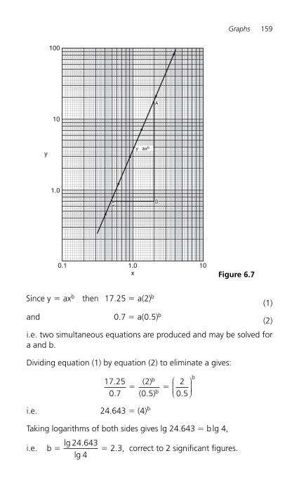
Graphs 159
Since y ax then a( )b b� �17 25 2. (1)
and 0 7 0 5. .� a( )b (2)
i.e. two simultaneous equations are produced and may be solved for a and b.
Dividing equation (1) by equation (2) to eliminate a gives:
17 250 7
20 5
20 5
.
.( )
( . ) .� �
b
b
b⎛⎝⎜⎜⎜
⎞⎠⎟⎟⎟⎟
i.e. 24.643 � (4) b
Taking logarithms of both sides gives lg 24.643 � b lg 4,
i.e. blg
lg� �
24 6434
2 3.
. , correct to 2 significant figures.
100
10
1.0
y
x0.1 1.0 10
A
BC
y axb
Figure 6.7
160 Engineering Mathematics Pocket Book
Substituting b � 2.3 in equation (1) gives: 17.25 � a(2) 2.3 , i.e.
a � � �
17 252
17 254 925
3 52 3
.( )
..
..
correct to 2 significant figures.
Hence the law of the graph is: y � 3.5x 2.3
Application: The pressure p and volume v of a gas are believed to be related by a law of the form p � cv n, where c and n are constants. Experimental values of p and corresponding values of v obtained in a laboratory are:
p (Pascals) 2.28 � 105 8.04 � 10 5 2.03 � 10 6 5.05 � 10 6 1.82 � 10 7
v (m 3 ) 3.2 � 10 � 2 1.3 � 10 � 2 6.7 � 10 � 3 3.5 � 10 � 3 1.4 � 10 � 3
Verify that the law is true and determine approximate values of c and n
Since p � cv n, then lg p � n lg v � lg c, which is of the form Y � mX � c, showing that to produce a straight line graph, lg p is plotted vertically against lg v horizontally. The co-ordinates are plotted on ‘log 3 cycle � 2 cycle ’ graph paper as shown in Figure 6.8 . With the data expressed in standard form, the axes are marked in stand-ard form also. Since a straight line results the law p � cv n is verified.
The straight line has a negative gradient and the value of the g radient is given
by:ABBC
unitsunits
. Hence n� � �1410
1 4. �1.4
Selecting any point on the straight line, say point C, having co-ordinates (2.63 � 10 � 2, 3 � 10 5), and substituting these values in p � cv n gives: 3 � 10 5 � c(2.63 � 10 � 2 ) � 1.4
Hence,
c ��
��
�
��
��
� � �
3 102 63 10
3 100 0263
3 101 63 10
5
2 1 4
5
1 4
5
2
( . ) ( . )
.
. .
18400, correct to 3 significant figures.
Hence the law of the graph is: p � 1840v � 1.4 or pv1.4 � 1840
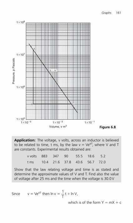
Graphs 161
Since v � Ve t/T then ln lnv V� �1T
t ,
which is of the form Y � mX � c
1�10�21�10�31�105
1�106
1�107
1�108
1�10�1
Volume, v m3
Pre
ssur
e, p
Pas
cals
A
CB
p � cvn
Figure 6.8
Application: The voltage, v volts, across an inductor is believed to be related to time, t ms, by the law v � Ve t/T, where V and T are constants. Experimental results obtained are:
v volts 883 347 90 55.5 18.6 5.2
t ms 10.4 21.6 37.8 43.6 56.7 72.0
Show that the law relating voltage and time is as stated and determine the approximate values of V and T. Find also the value of voltage after 25 ms and the time when the voltage is 30.0 V
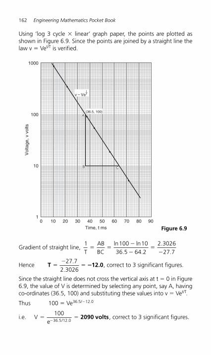
162 Engineering Mathematics Pocket Book
Using ‘log 3 cycle � linear ’ graph paper, the points are plotted as shown in Figure 6.9 . Since the points are joined by a straight line the law v � Ve t/T is verified.
1000
100
Vol
tage
, v v
olts
10
10 10 20 30 40 50
Time, t ms60 70 80 90
(36.5, 100)
CB
A
v�VeTt
Figure 6.9
Gradient of straight line, 1 100 10
36 5 64 22 3026
27 7TABBC
ln ln� �
�
��
�. ..
.
Hence T 12.0��
�27 7
2 3026.
.� , correct to 3 significant figures.
Since the straight line does not cross the vertical axis at t � 0 in Figure 6.9, the value of V is determined by selecting any point, say A, having co-ordinates (36.5, 100) and substituting these values into v � Ve t/T .
Thus 100 � Ve 36.5/ � 12.0
i.e. V
e /� �
�
10036 5 12 0. .
2090 volts , correct to 3 significant figures.
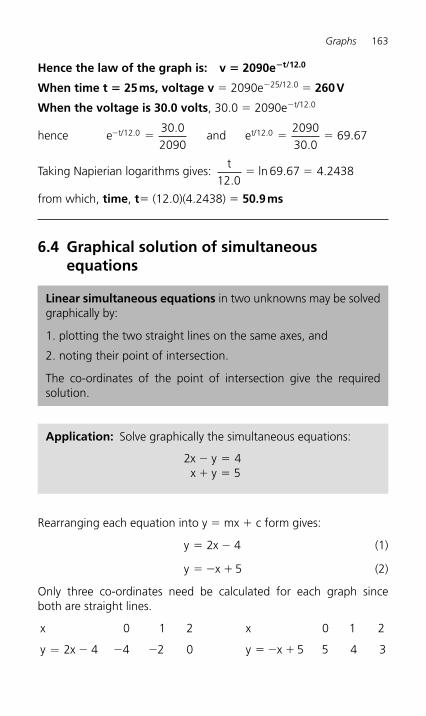
Graphs 163
Hence the law of the graph is: v � 2090e � t/12.0
When time t � 25 ms, voltage v � 2090e � 25/12.0 � 260 V
When the voltage is 30.0 volts , 30.0 � 2090e � t/12.0
hence e and et/ t/� � � �12 0 12 030 02090
209030 0
69 67. ...
.
Taking Napierian logarithms gives: t
ln12 0
69 67 4 2438.
. .� �
from which, time , t � (12.0)(4.2438) � 50.9 ms
6.4 Graphical solution of simultaneous equations
Linear simultaneous equations in two unknowns may be solved graphically by:
1. plotting the two straight lines on the same axes, and
2. noting their point of intersection.
The co-ordinates of the point of intersection give the required solution.
Application: Solve graphically the simultaneous equations:
2 45
x yx y
� �� �
Rearranging each equation into y � mx � c form gives:
y x� �2 4 (1)
y x� � � 5 (2)
Only three co-ordinates need be calculated for each graph since both are straight lines.
x 0 1 2 x
y x y x
0 1 2
2 4 4 2 0 5 5 4 3= � � � � � �
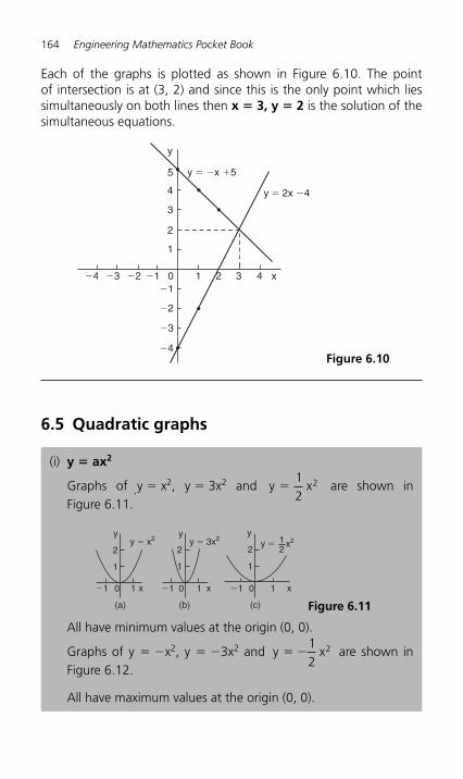
164 Engineering Mathematics Pocket Book
Each of the graphs is plotted as shown in Figure 6.10 . The point of intersection is at (3, 2) and since this is the only point which lies simultaneously on both lines then x � 3, y � 2 is the solution of the simultaneous equations.
�4 �3 �2 �1 10�1
1
3
2
4
5
�2
�3
�4
2 3 4
y � 2x �4
y � �x �5
y
x
Figure 6.10
6.5 Quadratic graphs
(i) y � ax2
Graphs of y � x 2, y � 3x2 and y x�12
2 are shown in Figure 6.11.
.
All have minimum values at the origin (0, 0).
Graphs of y � � x 2, y � � 3x 2 and y x� �12
2 are shown in Figure 6.12 .
All have maximum values at the origin (0, 0).
2
1
0�1 1
2
1
0�1 1
2
1
0�1 1
(a) (b) (c)
y � x2 y � 3x2 12
y � x2y
x x x
y y
Figure 6.11
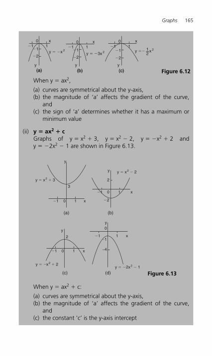
Graphs 165
When y � ax2 ,
(a) curves are symmetrical about the y-axis, (b) the magnitude of ‘ a ’ affects the gradient of the curve,
and (c) the sign of ‘ a ’ determines whether it has a maximum or
minimum value
(ii) y � ax2 � c Graphs of y � x 2 � 3, y � x 2 � 2, y � � x 2 � 2 and y � � 2x2 � 1 are shown in Figure 6.13 .
When y � ax2 � c:
(a) curves are symmetrical about the y-axis, (b) the magnitude of ‘ a ’ affects the gradient of the curve,
and (c) the constant ‘ c ’ is the y-axis intercept
3
�1
�1
�1 1
�1 1
1
1
(a)
0
(b)
0
�2
2
y
2
x
(c)
0
(d)
−1
−4
0
y � x2 � 3
y � �x2 � 2y � �2x2 � 1
y � x2 � 2y
y
y
x
x
x
Figure 6.13
(b) (c)(a) (b) (c)(a)
0
�1�1 1
�2
0
�1�1 1
�2y � �x 2
y � �3x 212
y �� x 2
0
�1�1 1
y
xx x
yy
�2
Figure 6.12
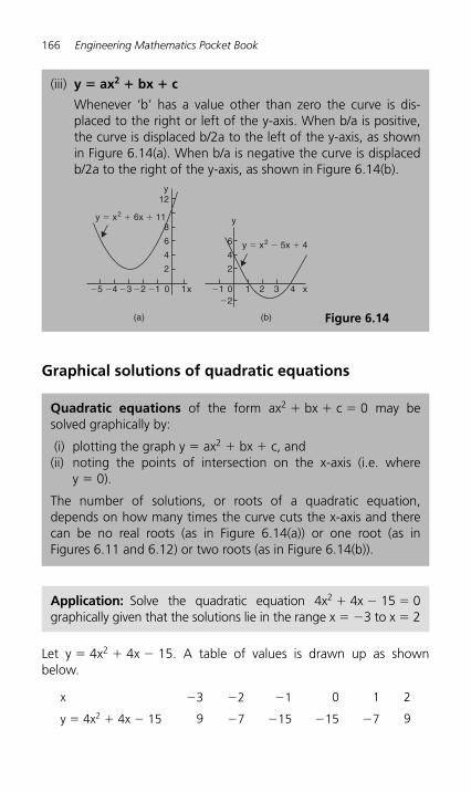
166 Engineering Mathematics Pocket Book
Graphical solutions of quadratic equations
(iii) y � ax 2 � bx � c
Whenever ‘ b ’ has a value other than zero the curve is dis-placed to the right or left of the y-axis. When b/a is positive, the curve is displaced b/2a to the left of the y-axis, as shown in Figure 6.14(a). When b/a is negative the curve is displaced b/2a to the right of the y-axis, as shown in Figure 6.14(b) .
�5 �4 �3 �2�2
0 1 2 3 4
2
4
6
�1 �10 1x x
y
y � x2 � 6x � 11
y � x2 � 5x � 4
2
4
6
8
12
(a) (b)
y
Figure 6.14
Quadratic equations of the form ax 2 � bx � c � 0 may be solved graphically by:
(i) plotting the graph y � ax 2 � bx � c, and (ii) noting the points of intersection on the x-axis (i.e. where
y � 0).
The number of solutions, or roots of a quadratic equation, depends on how many times the curve cuts the x-axis and there can be no real roots (as in Figure 6.14(a) ) or one root (as in Figures 6.11 and 6.12 ) or two roots (as in Figure 6.14(b) ).
Application: Solve the quadratic equation 4x 2 � 4x � 15 � 0 graphically given that the solutions lie in the range x � � 3 to x � 2
Let y � 4x 2 � 4x � 15. A table of values is drawn up as shown below.
x �3 �2 � 1 0 1 2
y � 4x 2 � 4x � 15 9 �7 �15 �15 � 7 9
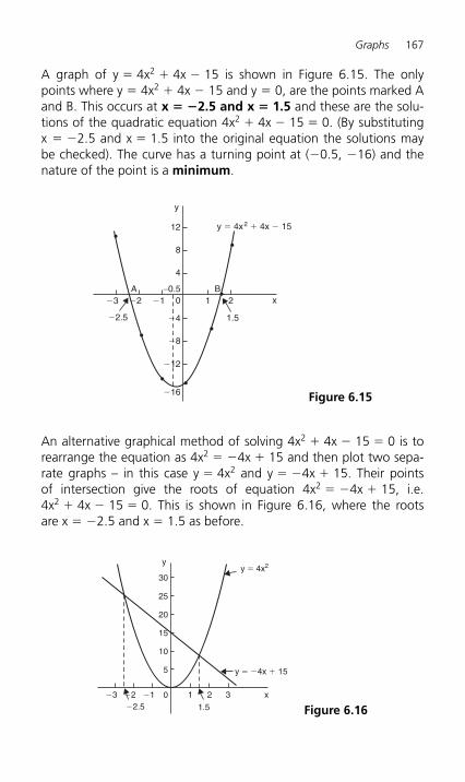
Graphs 167
A graph of y � 4x 2 � 4x � 15 is shown in Figure 6.15 . The only points where y � 4x 2 � 4x � 15 and y � 0, are the points marked A and B. This occurs at x � � 2.5 and x � 1.5 and these are the solu-tions of the quadratic equation 4x 2 � 4x � 15 � 0. (By substituting x � � 2.5 and x � 1.5 into the original equation the solutions may be checked). The curve has a turning point at ( �0.5, �16) and the nature of the point is a minimum .
12
8
4
�3 �2
�2.5
�1 1 20−0.5
�4
�8
�12
�16
1.5
y � 4x2 � 4x � 15
BAx
y
Figure 6.15
An alternative graphical method of solving 4x 2 � 4x � 15 � 0 is to rearrange the equation as 4x 2 � � 4x � 15 and then plot two sepa-rate graphs – in this case y � 4x 2 and y � � 4x � 15. Their points of intersection give the roots of equation 4x 2 � � 4x � 15, i.e. 4x2 � 4x � 15 � 0. This is shown in Figure 6.16 , where the roots are x � � 2.5 and x � 1.5 as before.
30
25
20
15
10
5
0�3 �2 �1 1 2
1.5
3�2.5
y � �4x � 15
y � 4x2
x
y
Figure 6.16
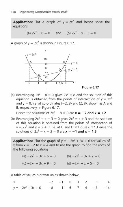
168 Engineering Mathematics Pocket Book
A graph of y � 2x 2 is shown in Figure 6.17 .
10
8
6
4
2
0�1 1 1.5 2�2
y � x � 3
y � 8
y � 2x2
x
y
A B
D
C
Figure 6.17
Application: Plot a graph of y � 2x 2 and hence solve the equations
(a) x and (b) x x2 8 0 2 3 02 2� � � � �
(a) Rearranging 2x 2 � 8 � 0 gives 2x 2 � 8 and the solution of this equation is obtained from the points of intersection of y � 2x 2 and y � 8, i.e. at co-ordinates ( �2, 8) and (2, 8), shown as A and B, respectively, in Figure 6.17 .
Hence the solutions of 2x 2 � 8 � 0 are x � � 2 and x � � 2
(b) Rearranging 2x 2 � x � 3 � 0 gives 2x 2 � x � 3 and the solution of this equation is obtained from the points of intersection of y � 2x 2 and y � x � 3, i.e. at C and D in Figure 6.17 . Hence the solutions of 2x 2 � x � 3 � 0 are x � � 1 and x � 1.5
Application: Plot the graph of y � � 2x 2 � 3x � 6 for values of x from x � � 2 to x � 4 and to use the graph to find the roots of the following equations
( ) ( )
( ) ( )
a x x b x x
c x x d x x
� � � � � � � �
� � � � � � � �
2 3 6 0 2 3 2 0
2 3 9 0 2 5 0
2 2
2 2
A table of values is drawn up as shown below.
x �2 � 1 0 1 2 3 4
y � � 2x 2 � 3x � 6 � 8 1 6 7 4 �3 � 14
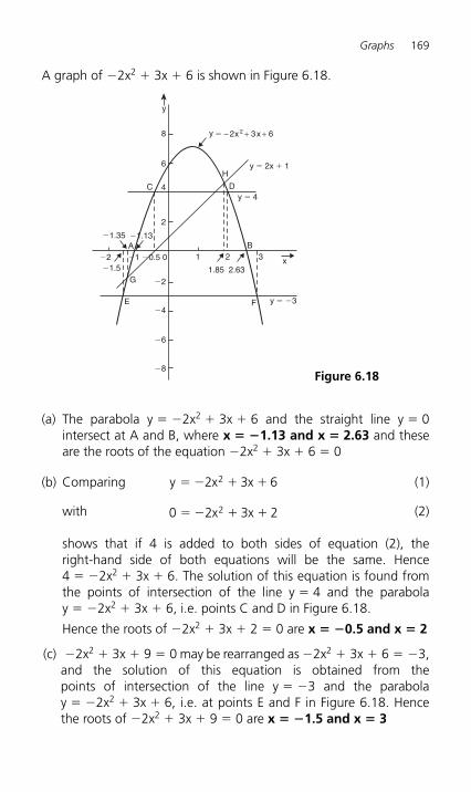
Graphs 169
A graph of �2x2 � 3x � 6 is shown in Figure 6.18 .
8 � − 2 2 + 3 + 6
6
4
2
�1.35 �1.13
�2 �1 �0.5�1.5
0 1 2 3
�2
�4
�6
�8
1.85 2.63
y � �3
y � 2x � 1
y � 4
y
x xy
C
A
G
E F
H
D
B
x
Figure 6.18
(a) The parabola y � � 2x2 � 3x � 6 and the straight line y � 0 intersect at A and B, where x � � 1.13 and x � 2.63 and these are the roots of the equation � 2x 2 � 3x � 6 � 0
(b) Comparing y x x� � � �2 3 62 (1)
with 0 2 3 22� � � �x x (2)
shows that if 4 is added to both sides of equation (2), the right-hand side of both equations will be the same. Hence 4 � � 2x2 � 3x � 6. The solution of this equation is found from the points of intersection of the line y � 4 and the parabola y � � 2x2 � 3x � 6, i.e. points C and D in Figure 6.18 .
Hence the roots of � 2x2 � 3x � 2 � 0 are x � � 0.5 and x � 2
(c) � 2x2 � 3x � 9 � 0 may be rearranged as �2x2 � 3x � 6 � � 3,and the solution of this equation is obtained from the points of intersection of the line y � � 3 and the parabola y � � 2x2 � 3x � 6, i.e. at points E and F in Figure 6.18 . Hence the roots of �2x2 � 3x � 9 � 0 are x � � 1.5 and x � 3
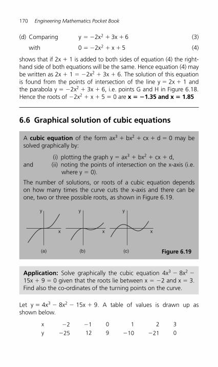
170 Engineering Mathematics Pocket Book
(d) Comparing y x x� � � �2 3 62 (3)
with 0 2 52� � � �x x (4)
shows that if 2x � 1 is added to both sides of equation (4) the right-hand side of both equations will be the same. Hence equation (4) may be written as 2x � 1 � � 2x2 � 3x � 6. The solution of this equation is found from the points of intersection of the line y � 2x � 1 and the parabola y � � 2x2 � 3x � 6, i.e. points G and H in Figure 6.18 .Hence the roots of �2x2 � x � 5 � 0 are x � � 1.35 and x � 1.85
6.6 Graphical solution of cubic equations
A cubic equation of the form ax 3 � bx 2 � cx � d � 0 may be solved graphically by:
(i) plotting the graph y � ax3 � bx 2 � cx � d, and (ii) noting the points of intersection on the x-axis (i.e.
where y � 0).
The number of solutions, or roots of a cubic equation depends on how many times the curve cuts the x-axis and there can be one, two or three possible roots, as shown in Figure 6.19 .
Application: Solve graphically the cubic equation 4x 3 � 8x 2 � 15x � 9 � 0 given that the roots lie between x � � 2 and x � 3.Find also the co-ordinates of the turning points on the curve.
(a) (b) (c)
y y y
xxx
Figure 6.19
Let y � 4x 3 � 8x 2 � 15x � 9. A table of values is drawn up as shown below.
x �2 � 1 0 1 2 3
y � 25 12 9 �10 � 21 0
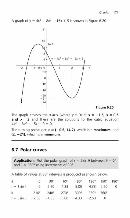
Graphs 171
A graph of y � 4x 3 � 8x 2 � 15x � 9 is shown in Figure 6.20 .
Application: Plot the polar graph of r � 5 sin θ between θ � 0° and θ � 360° using increments of 30°
A table of values at 30 o intervals is produced as shown below.
θ 0 30° 60° 90° 120° 150° 180°
r � 5 sin θ 0 2.50 4.33 5.00 4.33 2.50 0
θ 210° 240° 270° 300° 330° 360°
r � 5 sin θ �2.50 �4.33 �5.00 �4.33 � 2.50 0
�2 �1 �0.6 1 2 30
1614.2
12
8
4
�4
�8
�12
�16
�20�21�24
y � 4x3 � 8x2 � 15x � 9
y
x
Figure 6.20
The graph crosses the x-axis (where y � 0) at x � � 1.5, x � 0.5 and x � 3 and these are the solutions to the cubic equation 4x3 � 8x 2 � 15x � 9 � 0.
The turning points occur at (�0.6, 14.2), which is a maximum, and (2, � 21) , which is a minimum .
6.7 Polar curves
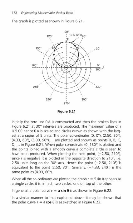
172 Engineering Mathematics Pocket Book
The graph is plotted as shown in Figure 6.21 .
D
C
BA
0 1 2 3 4 5
F
E
120°
150°
180°
210°
240°270°
300°
330°
360°0°
30°
60°r � 5 sin θ90°
Figure 6.21
Initially the zero line 0 A is constructed and then the broken lines in Figure 6.21 at 30° intervals are produced. The maximum value of r is 5.00 hence 0 A is scaled and circles drawn as shown with the larg-est at a radius of 5 units. The polar co-ordinates (0, 0°), (2.50, 30°), (4.33, 60°), (5.00, 90°) …. are plotted and shown as points 0, B, C, D, … in Figure 6.21 . When polar co-ordinate (0, 180°) is plotted and the points joined with a smooth curve a complete circle is seen to have been produced. When plotting the next point, ( �2.50, 210°), since r is negative it is plotted in the opposite direction to 210°, i.e. 2.50 units long on the 30° axis. Hence the point ( �2.50, 210°) is equivalent to the point (2.50, 30°). Similarly, ( �4.33, 240°) is the same point as (4.33, 60°).
When all the co-ordinates are plotted the graph r � 5 sin θ appears as a single circle; it is, in fact, two circles, one on top of the other.
In general, a polar curve r � a sin θ is as shown in Figure 6.22 .
In a similar manner to that explained above, it may be shown that the polar curve r � a cos θ is as sketched in Figure 6.23 .
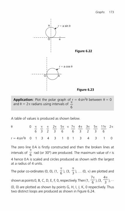
Graphs 173
A table of values is produced as shown below.
θ 0
π6
π3
π2
23π
56π
π
76π
43π
32π
53π
116π
2π
r � 4 sin 2 θ 0 1 3 4 3 1 0 1 3 4 3 1 0
The zero line 0 A is firstly constructed and then the broken lines at
intervals ofπ6
rad (or 30°) are produced. The maximum value of r is
4 hence 0 A is scaled and circles produced as shown with the largest at a radius of 4 units.
The polar co-ordinates (0, 0), (1, π6 ), (3,
π3 ), … (0, π) are plotted and
shown as points 0, B, C, D, E, F, 0, respectively. Then (1, 76π
), (3, 43π
), …
(0, 0) are plotted as shown by points G, H, I, J, K, 0 respectively. Thus two distinct loops are produced as shown in Figure 6.24 .
Application: Plot the polar graph of r � 4 sin 2 θ between θ � 0 and θ � 2 π radians using intervals of π
6
a
aO
r � a sin θ
Figure 6.22
aO
r � a cos θ
Figure 6.23
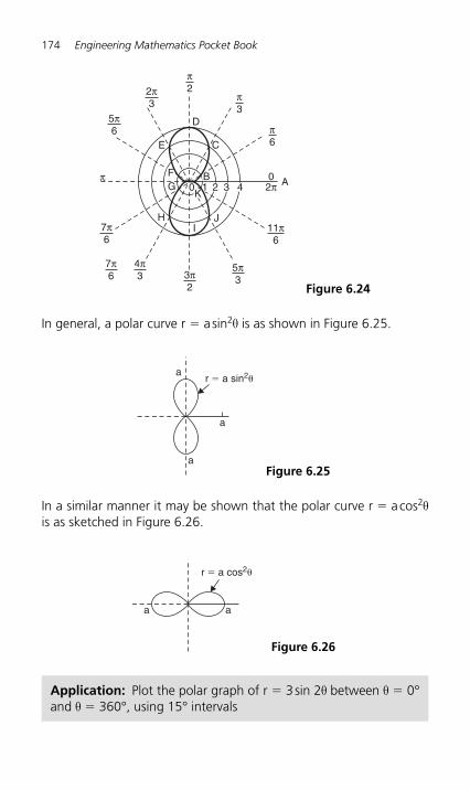
174 Engineering Mathematics Pocket Book
In general, a polar curve r � a sin 2 θ is as shown in Figure 6.25 .
aa
r � a cos2�
Figure 6.26
a
a
ar � a sin2�
Figure 6.25
C
D
E
1 2 3F
H JI
K
BG 4 2π
11π6
A0
5π33π
2
4π3
7π6
7π6
5π6
2π3
π2
π3
π6
π0
Figure 6.24
In a similar manner it may be shown that the polar curve r � a cos 2 θ is as sketched in Figure 6.26 .
Application: Plot the polar graph of r � 3 sin 2 θ between θ � 0° and θ � 360°, using 15° intervals
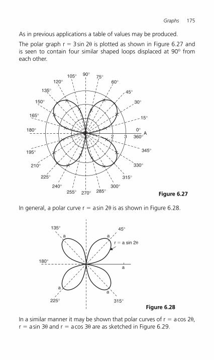
Graphs 175
As in previous applications a table of values may be produced.
The polar graph r � 3 sin 2 θ is plotted as shown in Figure 6.27 and is seen to contain four similar shaped loops displaced at 90 o from each other.
0
120°105° 75°
45°
15°
A
150°
180°
210°
240°270° 285°255°
225°
195°
165°
135°
300°
330°
360°
345°
315°
0°
30°
60°
90°
1 2 3
Figure 6.27
In general, a polar curve r � a sin 2 θ is as shown in Figure 6.28 .
45°
a
aa
a a
180°
225°
135°
315°
r � a sin 2�
Figure 6.28
In a similar manner it may be shown that polar curves of r � a cos 2 θ , r � a sin 3 θ and r � a cos 3 θ are as sketched in Figure 6.29 .
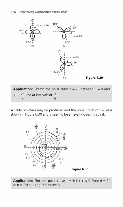
176 Engineering Mathematics Pocket Book
A table of values may be produced and the polar graph of r � 2 θ is shown in Figure 6.30 and is seen to be an ever-increasing spiral.
2π
11π6
0
5π3
3π2
4π3
7π6
5π6
2π3
π2
r � 2�
π3
π6
π15129630
Figure 6.30
90°
30°
0°
a
a
a
aa
a
a
a
a
a
a
180°
150°
120°
240°
270°
(a) (b)
(c)
270°
r � a cos 2�
r � a sin 3�
r � a cos 3�
Figure 6.29
Application: Sketch the polar curve r � 2 θ between θ � 0 and
θπ
�52
rad at intervals of π6
Application: Plot the polar curve r � 5(1 � cos θ) from θ � 0° to θ � 360°, using 30° intervals
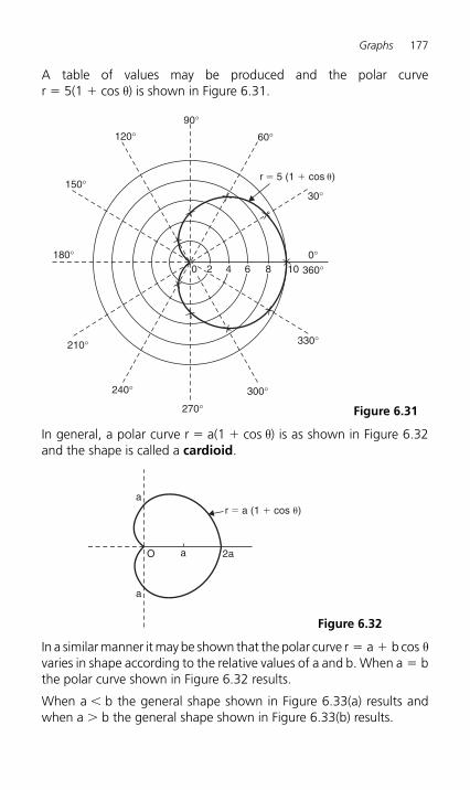
Graphs 177
In general, a polar curve r � a(1 � cos θ) is as shown in Figure 6.32 and the shape is called a cardioid .
a
a
a
O 2a
r � a (1 � cos �)
Figure 6.32
A table of values may be produced and the polar curve r � 5(1 � cos θ ) is shown in Figure 6.31 .
120°
150°
180°
210°
240°
270°
300°
330°
360°0°
30°
r � 5 (1 � cos �)
60°
90°
0 2 4 6 8 10
Figure 6.31
In a similar manner it may be shown that the polar curve r � a � b cos θ varies in shape according to the relative values of a and b. When a � b the polar curve shown in Figure 6.32 results.
When a b the general shape shown in Figure 6.33(a) results and when a b the general shape shown in Figure 6.33(b) results.
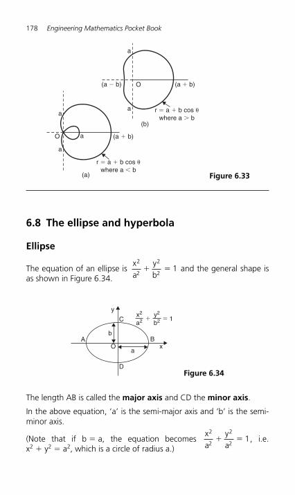
178 Engineering Mathematics Pocket Book
6.8 The ellipse and hyperbola
Ellipse
The equation of an ellipse isxa
yb
2
2
2
21� � and the general shape is
as shown in Figure 6.34 .
bA
C
D
B
a
y
xO
1� �a2x2
b2y2
Figure 6.34
a
a
a
O (a � b)
r � a � b cos �where a b
a
a
O(a � b) (a � b)
(a)
(b)
r � a � b cos �where a b
Figure 6.33
The length AB is called the major axis and CD the minor axis .
In the above equation, ‘ a ’ is the semi-major axis and ‘ b ’ is the semi-minor axis.
(Note that if b � a, the equation becomesxa
ya
2
2
2
21� � , i.e.
x2 � y 2 � a 2 , which is a circle of radius a.)
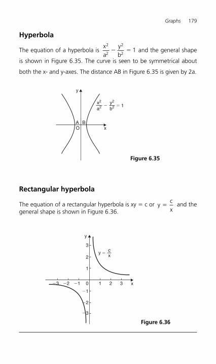
Graphs 179
Hyperbola
The equation of a hyperbola isxa
yb
2
2
2
21� � and the general shape
is shown in Figure 6.35 . The curve is seen to be symmetrical about
both the x- and y-axes. The distance AB in Figure 6.35 is given by 2a.
BAO x
y
1� �a2x2
b2y2
Figure 6.35
Rectangular hyperbola
The equation of a rectangular hyperbola is xy � c or ycx
� and the general shape is shown in Figure 6.36 .
1�1
�1
1
2
3
�2
�3
�2�3 0 2 3 x
y
y � xc
Figure 6.36
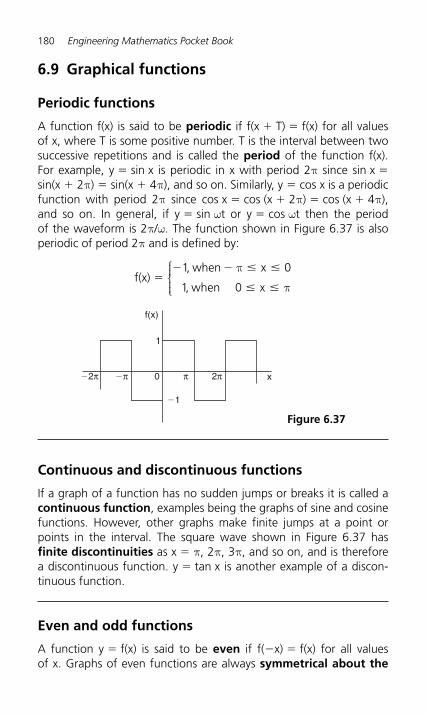
180 Engineering Mathematics Pocket Book
6.9 Graphical functions
Periodic functions
A function f(x) is said to be periodic if f(x � T) � f(x) for all values of x, where T is some positive number. T is the interval between two successive repetitions and is called the period of the function f(x). For example, y � sin x is periodic in x with period 2 π since sin x � sin(x � 2 π ) � sin(x � 4 π), and so on. Similarly, y � cos x is a periodic function with period 2 π since cos x � cos (x � 2 π ) � cos (x � 4 π ), and so on. In general, if y � sin ωt or y � cos ωt then the period of the waveform is 2 π / ω. The function shown in Figure 6.37 is also periodic of period 2 π and is defined by:
f(x), when x
when x�
� � � �
� �
1 0
1 0
π
π,
⎧⎨⎪⎪
⎩⎪⎪
0
1
�1
�2π �π π 2π
f(x)
x
Figure 6.37
Continuous and discontinuous functions
If a graph of a function has no sudden jumps or breaks it is called a continuous function, examples being the graphs of sine and cosine functions. However, other graphs make finite jumps at a point or points in the interval. The square wave shown in Figure 6.37 has finite discontinuities as x � π, 2 π, 3 π, and so on, and is therefore a discontinuous function. y � tan x is another example of a discon-tinuous function.
Even and odd functions
A function y � f(x) is said to be even if f( � x) � f(x) for all values of x. Graphs of even functions are always symmetrical about the
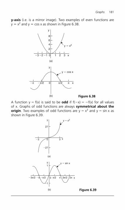
Graphs 181
y-axis (i.e. is a mirror image). Two examples of even functions are y � x 2 and y � cos x as shown in Figure 6.38 .
�3 �2 �1 10 2 3
2
4
6
8
(a)
0 π�π
(b)
y � cos x
y � x2
y
y
�π/2 π/2
x
x
Figure 6.38
A function y � f(x) is said to be odd if f( � x) � �f(x) for all values of x. Graphs of odd functions are always symmetrical about the origin. Two examples of odd functions are y � x 3 and y � sin x as shown in Figure 6.39 .
�3 0 3
27
y
�27
(a)
�3π/2 3π/2 2π�π/2 π/2 π�π 0
1
�1
(b)
y � x3
y � sin xy
x
x
Figure 6.39
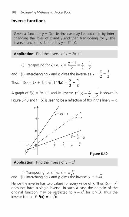
182 Engineering Mathematics Pocket Book
Inverse functions
Given a function y � f(x), its inverse may be obtained by inter-changing the roles of x and y and then transposing for y. The inverse function is denoted by y � f � 1 (x).
Application: Find the inverse of y � 2x � 1
(i) Transposing for x, i.e. x ��
� �y y1
2 212
and (ii) interchanging x and y, gives the inverse as yx
� �2
12
Thus if f(x) � 2x � 1, then f� � �1(x)x2
12
A graph of f(x) � 2x � 1 and its inverse f (x)x2
12
1� � � is shown in
Figure 6.40 and f � 1(x) is seen to be a reflection of f(x) in the line y � x.
1
0
2
�1 1 2 3 4 x
y
�1
4
y �
y � xy � 2x � 1
�2x
21
Figure 6.40
(i) Transposing for x, i.e. x y� and (ii) interchanging x and y, gives the inverse y x�
Hence the inverse has two values for every value of x. Thus f(x) � x 2 does not have a single inverse. In such a case the domain of the original function may be restricted to y � x 2 for x 0. Thus the inverse is then f (x) x1� � �
Application: Find the inverse of y � x 2
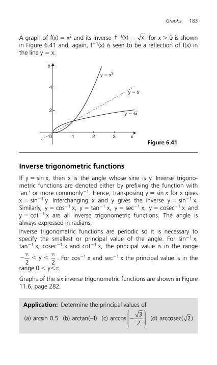
Graphs 183
A graph of f(x) � x 2 and its inverse f (x) x1� � for x 0 is shown in Figure 6.41 and, again, f � 1(x) is seen to be a reflection of f(x) in the line y � x.
Inverse trigonometric functions
If y � sin x, then x is the angle whose sine is y. Inverse trigono-metric functions are denoted either by prefixing the function with ‘ arc ’ or more commonly � 1. Hence, transposing y � sin x for x gives x � sin � 1 y. Interchanging x and y gives the inverse y � sin � 1 x. Similarly, y � cos � 1 x, y � tan � 1 x, y � sec � 1 x, y � cosec � 1 x and y � cot � 1 x are all inverse trigonometric functions. The angle is always expressed in radians. Inverse trigonometric functions are periodic so it is necessary to specify the smallest or principal value of the angle. For sin � 1 x, tan � 1 x, cosec � 1 x and cot � 1 x, the principal value is in the range
� π π2 2
y . For cos � 1 x and sec � 1 x the principal value is in the
range 0 y π .
Graphs of the six inverse trigonometric functions are shown in Figure 11.6, page 282.
10
2
4
2 3 x
y
y � x2
y � x
y � x
Figure 6.41
Application: Determine the principal values of
(a) arcsin (b) arctan( (c) arccos (d) arcc0 5 13
2. )� �
⎛
⎝⎜⎜⎜⎜
⎞
⎠⎟⎟⎟⎟⎟
oosec( )2
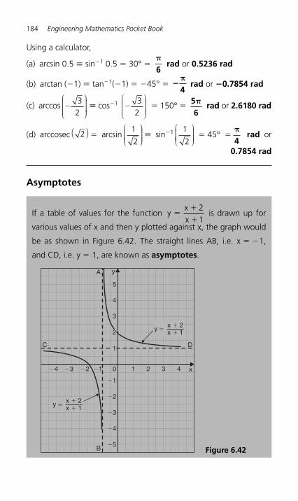
184 Engineering Mathematics Pocket Book
Using a calculator,
(a) arcsin 0.5 � sin � 1 0.5 � 30° � π6
rad or 0.5236 rad
(b) arctan ( � 1) � tan � 1 ( � 1) � � 45° � �π4
rad or � 0.7854 rad
(c) arccos �3
2
⎛
⎝⎜⎜⎜⎜
⎞
⎠⎟⎟⎟⎟⎟
� cos � 1 �3
2
⎛
⎝⎜⎜⎜⎜
⎞
⎠⎟⎟⎟⎟⎟
� 150° � 56π rad or 2.6180 rad
(d) arccosec 2( ) � arcsin 1
2
⎛
⎝⎜⎜⎜⎜
⎞
⎠⎟⎟⎟⎟ � sin � 1
1
2
⎛
⎝⎜⎜⎜⎜
⎞
⎠⎟⎟⎟⎟ � 45° �
π4
rad or
0.7854 rad
Asymptotes
If a table of values for the function yxx
��
�
21
is drawn up for
various values of x and then y plotted against x, the graph would
be as shown in Figure 6.42 . The straight lines AB, i.e. x � � 1,
and CD, i.e. y � 1, are known as asymptotes.
4321�1
�1
�2
�3
�4
�5
�2�3�4 0
1
2
3
4
5
y
x
C D
B
A
y �x � 2x � 1
y �x � 2x � 1
Figure 6.42
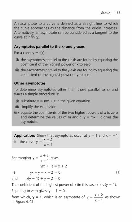
Graphs 185
Rearranging yxx
��
�
21
gives:
y(x � 1) � x � 2
i.e. yx y x� � � �2 0 (1)
and x(y � 1) � y � 2 � 0
The coefficient of the highest power of x (in this case x 1 ) is (y � 1).
Equating to zero gives: y � 1 � 0
from which, y � 1, which is an asymptote of yxx
��
�
21
as shown in Figure 6.42 .
An asymptote to a curve is defined as a straight line to which the curve approaches as the distance from the origin increases. Alternatively, an asymptote can be considered as a tangent to the curve at infinity.
Asymptotes parallel to the x- and y-axes
For a curve y � f(x):
(i) the asymptotes parallel to the x-axis are found by equating the coefficient of the highest power of x to zero
(ii) the asymptotes parallel to the y-axis are found by equating the coefficient of the highest power of y to zero
Other asymptotes
To determine asymptotes other than those parallel to x- and y-axes a simple procedure is:
(i) substitute y � mx � c in the given equation
(ii) simplify the expression
(iii) equate the coefficients of the two highest powers of x to zero and determine the values of m and c. y � mx � c gives the asymptote.
Application: Show that asymptotes occur at y � 1 and x � � 1
for the curve yxx
��
�
21
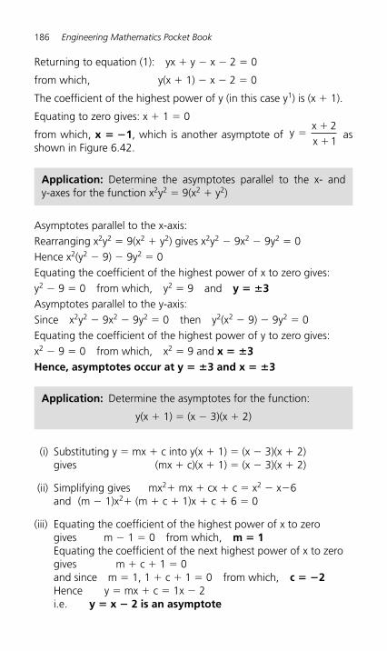
186 Engineering Mathematics Pocket Book
Returning to equation (1): yx � y � x � 2 � 0
from which, y(x � 1) � x � 2 � 0
The coefficient of the highest power of y (in this case y 1 ) is (x � 1).
Equating to zero gives: x � 1 � 0
from which, x � � 1, which is another asymptote of yxx
��
�
21
as shown in Figure 6.42 .
Application: Determine the asymptotes parallel to the x- and y-axes for the function x 2 y 2 � 9(x 2 � y 2 )
Asymptotes parallel to the x-axis: Rearranging x 2 y 2 � 9(x 2 � y 2 ) gives x 2 y 2 � 9x2 � 9y 2 � 0 Hence x 2 (y 2 � 9) � 9y 2 � 0 Equating the coefficient of the highest power of x to zero gives: y 2 � 9 � 0 from which, y 2 � 9 and y � � 3 Asymptotes parallel to the y-axis: Since x 2 y 2 � 9x 2 � 9y 2 � 0 then y 2 (x 2 � 9) � 9y 2 � 0 Equating the coefficient of the highest power of y to zero gives: x 2 � 9 � 0 from which, x 2 � 9 and x � � 3 Hence, asymptotes occur at y � � 3 and x � � 3
Application: Determine the asymptotes for the function:
y(x � 1) � (x � 3)(x � 2)
(i) Substituting y � mx � c into y(x � 1) � (x � 3)(x � 2) gives (mx � c)(x � 1) � (x � 3)(x � 2)
(ii) Simplifying gives mx 2 � mx � cx � c � x 2 � x � 6 and (m � 1)x 2 � (m � c � 1)x � c � 6 � 0
(iii) Equating the coefficient of the highest power of x to zero gives m � 1 � 0 from which, m � 1 Equating the coefficient of the next highest power of x to zero gives m � c � 1 � 0 and since m � 1, 1 � c � 1 � 0 from which, c � � 2 Hence y � mx � c � 1x � 2 i.e. y � x � 2 is an asymptote
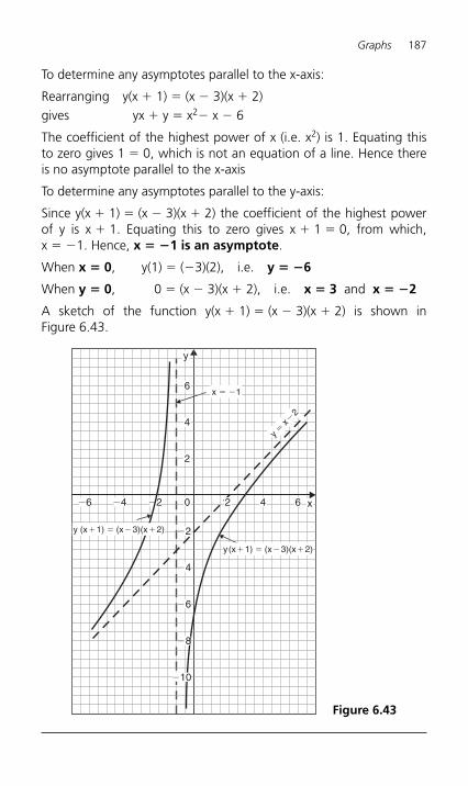
Graphs 187
To determine any asymptotes parallel to the x-axis:
Rearranging y(x � 1) � (x � 3)(x � 2)gives yx � y � x 2 � x � 6
The coefficient of the highest power of x (i.e. x 2) is 1. Equating this to zero gives 1 � 0, which is not an equation of a line. Hence there is no asymptote parallel to the x-axis
To determine any asymptotes parallel to the y-axis:
Since y(x � 1) � (x � 3)(x � 2) the coefficient of the highest power of y is x � 1. Equating this to zero gives x � 1 � 0, from which, x � � 1. Hence, x � � 1 is an asymptote .
When x � 0, y(1) � ( �3)(2), i.e. y � � 6
When y � 0 , 0 � (x � 3)(x � 2), i.e. x � 3 and x � � 2
A sketch of the function y(x � 1) � (x � 3)(x � 2) is shown in Figure 6.43 .
y
x
6
4
2
2 4 60�4 �2
�2
�4
�6
�8
�10
�6
x � �1
y (x�1) � (x�3)(x�2)
y(x�1) � (x�3)(x�2)
y � x
�2
Figure 6.43
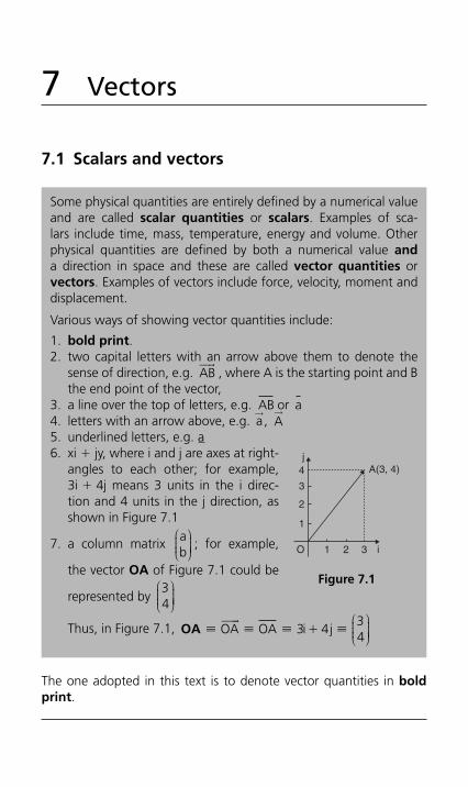
7 Vectors
7.1 Scalars and vectors
Some physical quantities are entirely defined by a numerical value and are called scalar quantities or scalars. Examples of sca-lars include time, mass, temperature, energy and volume. Other physical quantities are defined by both a numerical value and a direction in space and these are called vector quantities or vectors. Examples of vectors include force, velocity, moment and displacement.
Various ways of showing vector quantities include:
1. bold print. 2. two capital letters with an arrow above them to denote the
sense of direction, e.g. AB� ��
, where A is the starting point and B the end point of the vector,
3. a line over the top of letters, e.g. AB or a 4. letters with an arrow above, e.g. a
→ , A
→
5. underlined letters, e.g. a 6. xi � jy, where i and j are axes at right-
angles to each other; for example, 3i � 4j means 3 units in the i direc-tion and 4 units in the j direction, as shown in Figure 7.1
7. a column matrix ab
⎛⎝⎜⎜⎜
⎞⎠⎟⎟⎟⎟ ; for example,
the vector OA of Figure 7.1 could be
represented by 34
⎛⎝⎜⎜⎜
⎞⎠⎟⎟⎟⎟
Thus, in Figure 7.1 , OA � � � �OA OA i j� ���
3 434
�⎛⎝⎜⎜⎜
⎞⎠⎟⎟⎟⎟
A(3, 4)
i
j4
3
2
1
1 2 3O
Figure 7.1
The one adopted in this text is to denote vector quantities in boldprint .
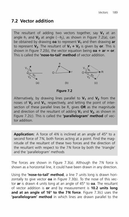
Vectors 189
7.2 Vector addition
The resultant of adding two vectors together, say V1 at an angle θ 1 and V2 at angle ( � θ 2), as shown in Figure 7.2(a) , can be obtained by drawing oa to represent V1 and then drawing ar to represent V2. The resultant of V1 � V2 is given by or. This is shown in Figure 7.2(b) , the vector equation being oa � ar � or . This is called the ‘ nose-to-tail ’ method of vector addition.
Alternatively, by drawing lines parallel to V1 and V2 from the noses of V2 and V1, respectively, and letting the point of inter-section of these parallel lines be R, gives OR as the magnitude and direction of the resultant of adding V1 and V2, as shown in Figure 7.2(c) . This is called the ‘ parallelogram ’ method of vec-tor addition.
Figure 7.2
θ1
θ2
(a)
V2
V1
(b)
a
rO
(c)
θ1
θ2V2
V1
O R
Application: A force of 4 N is inclined at an angle of 45 ° to a second force of 7 N, both forces acting at a point. Find the mag-nitude of the resultant of these two forces and the direction of the resultant with respect to the 7 N force by both the ‘ triangle ’ and the ‘ parallelogram ’ methods
The forces are shown in Figure 7.3(a) . Although the 7 N force is shown as a horizontal line, it could have been drawn in any direction.
Using the ‘ nose-to-tail ’ method, a line 7 units long is drawn hori-zontally to give vector oa in Figure 7.3(b) . To the nose of this vec-tor ar is drawn 4 units long at an angle of 45 ° to oa. The resultant of vector addition is or and by measurement is 10.2 units long and at an angle of 16 ° to the 7 N force. Figure 7.3(c) uses the ‘ parallelogram ’ method in which lines are drawn parallel to the
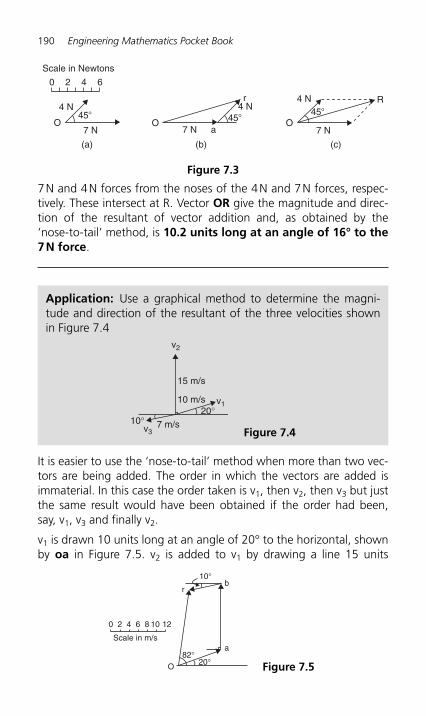
190 Engineering Mathematics Pocket Book
7 N and 4 N forces from the noses of the 4 N and 7 N forces, respec-tively. These intersect at R. Vector OR give the magnitude and direc-tion of the resultant of vector addition and, as obtained by the ‘ nose-to-tail ’ method, is 10.2 units long at an angle of 16 ° to the 7 N force .
20 4 6 8 10
10°b
r
a
O82°
20°
12
Scale in m/s
Figure 7.5
Figure 7.3
(a)
0 2 4 6
4 N
O45�
7 N
Scale in Newtons
(b)
4 Nr
45�
7 N aO
(c)
4 N45�
7 N
R
O
Application: Use a graphical method to determine the magni-tude and direction of the resultant of the three velocities shown in Figure 7.4
10°20°
7 m/s
15 m/s
10 m/s
v2
v1
v3 Figure 7.4
It is easier to use the ‘ nose-to-tail ’ method when more than two vec-tors are being added. The order in which the vectors are added is immaterial. In this case the order taken is v 1, then v 2, then v 3 but just the same result would have been obtained if the order had been, say, v 1 , v 3 and finally v 2 .
v 1 is drawn 10 units long at an angle of 20 ° to the horizontal, shown by oa in Figure 7.5 . v 2 is added to v 1 by drawing a line 15 units
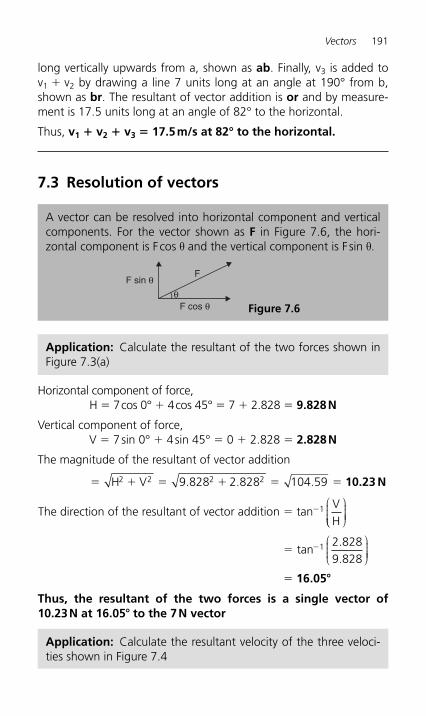
Vectors 191
long vertically upwards from a, shown as ab. Finally, v 3 is added to v1 � v 2 by drawing a line 7 units long at an angle at 190 ° from b, shown as br. The resultant of vector addition is or and by measure-ment is 17.5 units long at an angle of 82 ° to the horizontal.
Thus, v1 � v2 � v3 � 17.5 m/s at 82 ° to the horizontal.
7.3 Resolution of vectors
Application: Calculate the resultant of the two forces shown in Figure 7.3(a)
Horizontal component of force, H � 7 cos 0 ° � 4 cos 45 ° � 7 � 2.828 � 9.828 N
Vertical component of force, V � 7 sin 0 ° � 4 sin 45 ° � 0 � 2.828 � 2.828 N
The magnitude of the resultant of vector addition
� � � � � �H V2 2 2 29 828 2 828 104 59. . . 10.23 N
The direction of the resultant of vector addition tan� �1 VH
⎛⎝⎝⎜⎜⎜
⎞⎠⎟⎟⎟⎟
⎛⎝⎜⎜⎜
⎞⎠⎟⎟⎟⎟�
�
�tan 1 2 8289 828
.
.
16.05� Thus, the resultant of the two forces is a single vector of 10.23 N at 16.05 � to the 7 N vector
Application: Calculate the resultant velocity of the three veloci-ties shown in Figure 7.4
A vector can be resolved into horizontal component and vertical components. For the vector shown as F in Figure 7.6 , the hori-zontal component is F cos θ and the vertical component is F sin θ .
F sin θ
F cos θ
F
θ Figure 7.6
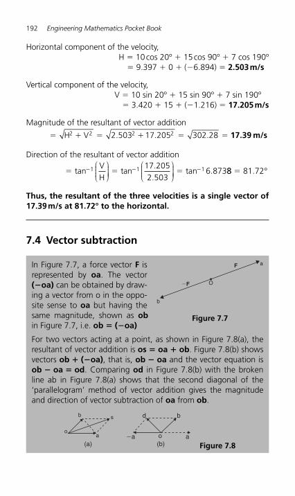
192 Engineering Mathematics Pocket Book
Horizontal component of the velocity, H � 10 cos 20º � 15 cos 90º � 7 cos 190º
� 9.397 � 0 � ( � 6.894) � 2.503 m/s
Vertical component of the velocity,V � 10 sin 20º � 15 sin 90º � 7 sin 190º
� 3.420 � 15 � ( � 1.216) � 17.205 m/s
Magnitude of the resultant of vector addition
� � � � � �H V2 2 2 22 503 17 205 302 28. . . 17.39 m/s
Direction of the resultant of vector addition
� � �� � �tan tan tan1 1 117 2052 503
6 873VH
⎛⎝⎜⎜⎜
⎞⎠⎟⎟⎟⎟
⎛⎝⎜⎜⎜
⎞⎠⎟⎟⎟⎟
..
. 88 81 72� . °
Thus, the resultant of the three velocities is a single vector of 17.39 m/s at 81.72 ° to the horizontal.
7.4 Vector subtraction
In Figure 7.7 , a force vector F is represented by oa. The vector (� oa) can be obtained by draw-ing a vector from o in the oppo-site sense to oa but having the same magnitude, shown as ob in Figure 7.7 , i.e. ob � ( �oa)
For two vectors acting at a point, as shown in Figure 7.8(a) , the resultant of vector addition is os � oa � ob. Figure 7.8(b) shows vectors ob � (� oa), that is, ob � oa and the vector equation is ob � oa � od. Comparing od in Figure 7.8(b) with the broken line ab in Figure 7.8(a) shows that the second diagonal of the ‘ parallelogram ’ method of vector addition gives the magnitude and direction of vector subtraction of oa from ob.
�F O
a
b
F
Figure 7.7
(b)a�a o
bd
(a)a
sb
o
Figure 7.8
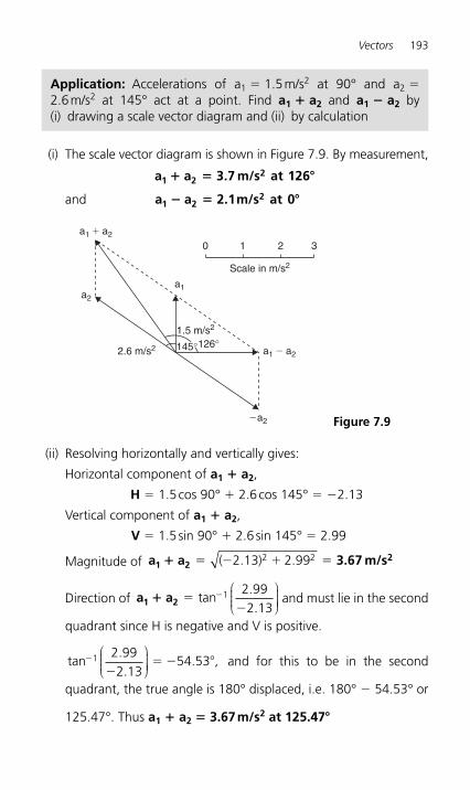
Vectors 193
(i) The scale vector diagram is shown in Figure 7.9 . By measurement,
a a 3.7 m/s at 1261 22� � �
and a a 2.1m/s at 01 22� � �
Scale in m/s2
2.6 m/s2
1.5 m/s2
126°
0 1 2 3
a1 � a2
a1 � a2
a2
�a2
a1
145°
Figure 7.9
Application: Accelerations of a 1 � 1.5 m/s 2 at 90 ° and a 2 � 2.6 m/s 2 at 145 ° act at a point. Find a1 � a 2 and a1 � a 2 by (i) drawing a scale vector diagram and (ii) by calculation
(ii) Resolving horizontally and vertically gives:
Horizontal component of a1 � a2 ,
H � 1.5 cos 90 ° � 2.6 cos 145 ° � � 2.13
Vertical component of a1 � a2 ,
V � 1.5 sin 90 ° � 2.6 sin 145 ° � 2.99
Magnitude of a a 3.67 m/s1 22� � � � �( . ) .2 13 2 992 2
Direction of a a1 2� ��
�tan 1 2 992 13..
⎛⎝⎜⎜⎜
⎞⎠⎟⎟⎟⎟ and must lie in the second
quadrant since H is negative and V is positive.
tan ,�
�� � �1 2 99
2 1354 53
..
.⎛⎝⎜⎜⎜
⎞⎠⎟⎟⎟⎟ and for this to be in the second
quadrant, the true angle is 180 ° displaced, i.e. 180 ° � 54.53 ° or
125.47 ° . Thus a1 � a2 � 3.67 m/s 2 at 125.47 �
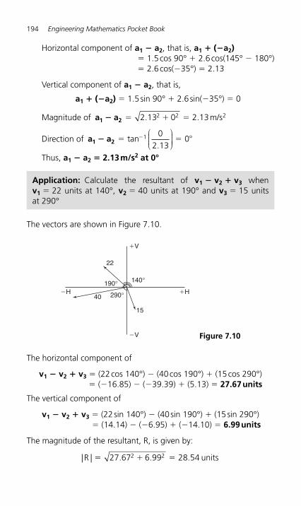
194 Engineering Mathematics Pocket Book
Horizontal component of a1 � a2 , that is, a1 � (� a 2 ) � 1.5 cos 90 ° � 2.6 cos(145 ° � 180 ° ) � 2.6 cos( � 35 ° ) � 2.13
Vertical component of a1 � a2 , that is,
a1 � (� a 2 ) � 1.5 sin 90 ° � 2.6 sin( � 35 ° ) � 0
Magnitude of a a1 2� � � �2 13 0 2 132 2 2. . m/s
Direction of a a1 2� � ��tan 1 02 13
0.
⎛⎝⎜⎜⎜
⎞⎠⎟⎟⎟⎟ �
Thus, a1 � a 2 � 2.13 m/s 2 at 0 °
15
22
40
190°
290°
140°
�V
�V
�H �H
Figure 7.10
Application: Calculate the resultant of v1 � v 2 � v 3 when v1 � 22 units at 140 °, v2 � 40 units at 190 ° and v3 � 15 units at 290 °
The vectors are shown in Figure 7.10 .
The horizontal component of
v1 � v 2 � v3 � (22 cos 140 ° ) � (40 cos 190 ° ) � (15 cos 290 ° ) � ( � 16.85) � ( � 39.39) � (5.13) � 27.67 units
The vertical component of
v1 � v 2 � v3 � (22 sin 140 ° ) � (40 sin 190 ° ) � (15 sin 290 ° ) � (14.14) � ( � 6.95) � ( � 14.10) � 6.99 units
The magnitude of the resultant, R, is given by:
| | . . .R � � �27 67 6 99 28 542 2 units
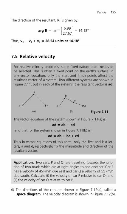
Vectors 195
The direction of the resultant, R , is given by :
arg R � ��tan 1 6 99
27 6714 18
..
.⎛⎝⎜⎜⎜
⎞⎠⎟⎟⎟⎟ °
Thus, v1 � v2 � v3 � 28.54 units at 14.18 °
7.5 Relative velocity
For relative velocity problems, some fixed datum point needs to be selected. This is often a fixed point on the earth’s surface. In any vector equation, only the start and finish points affect the resultant vector of a system. Two different systems are shown in Figure 7.11 , but in each of the systems, the resultant vector is ad.
The vector equation of the system shown in Figure 7.11(a) is:
ad � ab � bd
and that for the system shown in Figure 7.11(b) is:
ad � ab � bc � cd
Thus in vector equations of this form, only the first and last let-ters, a and d, respectively, fix the magnitude and direction of the resultant vector.
b
(a)
a d
Figure 7.11
b
(b)
a d
c
Application: Two cars, P and Q, are travelling towards the junc-tion of two roads which are at right angles to one another. Car P has a velocity of 45 km/h due east and car Q a velocity of 55 km/h due south. Calculate (i) the velocity of car P relative to car Q, and (ii) the velocity of car Q relative to car P
(i) The directions of the cars are shown in Figure 7.12(a) , called a space diagram. The velocity diagram is shown in Figure 7.12(b) ,
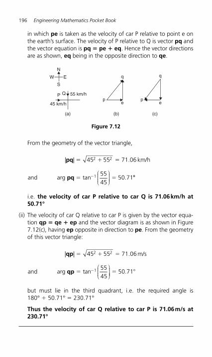
196 Engineering Mathematics Pocket Book
in which pe is taken as the velocity of car P relative to point e on the earth’s surface. The velocity of P relative to Q is vector pq and the vector equation is pq � pe � eq. Hence the vector directions are as shown, eq being in the opposite direction to qe .
Figure 7.12
P Q
N
S
45 km/h
E
55 km/h
(a)
W q
ep
(b)
q
ep
(c)
From the geometry of the vector triangle,
| | .
.
pq
pq
� � �
� ��
45 55 71 06
5545
50 71
2 2
1
km/h
and arg tan⎛⎝⎜⎜⎜
⎞⎠⎟⎟⎟⎟ ��
i.e. the velocity of car P relative to car Q is 71.06 km/h at 50.71 °
(ii) The velocity of car Q relative to car P is given by the vector equa-tion qp � qe � ep and the vector diagram is as shown in Figure 7.12(c), having ep opposite in direction to pe. From the geometry of this vector triangle:
| | .
.
qp
qp
� � �
� � ��
45 55 71 06
5545
50 71
2 2
1
m/s
and arg tan⎛⎝⎜⎜⎜
⎞⎠⎟⎟⎟⎟
but must lie in the third quadrant, i.e. the required angle is 180 ° � 50.71 ° � 230.71 °
Thus the velocity of car Q relative to car P is 71.06 m/s at 230.71 °
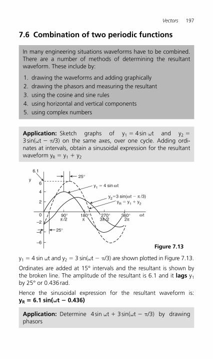
Vectors 197
7.6 Combination of two periodic functions
In many engineering situations waveforms have to be combined. There are a number of methods of determining the resultant waveform. These include by:
1. drawing the waveforms and adding graphically 2. drawing the phasors and measuring the resultant 3. using the cosine and sine rules 4. using horizontal and vertical components 5. using complex numbers
Application: Sketch graphs of y 1 � 4 sin ωt and y 2 � 3 sin( ω t � π/3) on the same axes, over one cycle. Adding ordi-nates at intervals, obtain a sinusoidal expression for the resultant waveform y R � y 1 � y 2
6y
6.1
4
2
0 90°π /2 3π /2
25°
25°
yR � y1 � y2
y2�3 sin(ω t � π /3)
y1 � 4 sin ω t
ω t
–2
–4
–6
2ππ180° 270° 360°
Figure 7.13
y1 � 4 sin ωt and y 2 � 3 sin( ωt � π/3) are shown plotted in Figure 7.13 .
Ordinates are added at 15 ° intervals and the resultant is shown by the broken line. The amplitude of the resultant is 6.1 and it lags y 1 by 25 ° or 0.436 rad.
Hence the sinusoidal expression for the resultant waveform is: yR � 6.1 sin( ω t � 0.436)
Application: Determine 4 sin ω t � 3 sin( ω t � π/3) by drawing phasors
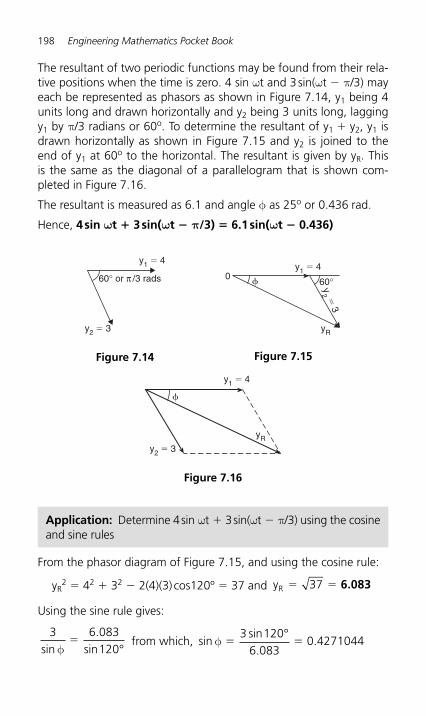
198 Engineering Mathematics Pocket Book
The resultant of two periodic functions may be found from their rela-tive positions when the time is zero. 4 sin ωt and 3 sin( ω t � π/3) may each be represented as phasors as shown in Figure 7.14 , y 1 being 4 units long and drawn horizontally and y 2 being 3 units long, lagging y1 by π/3 radians or 60 o. To determine the resultant of y 1 � y 2, y 1 is drawn horizontally as shown in Figure 7.15 and y 2 is joined to the end of y 1 at 60 o to the horizontal. The resultant is given by y R. This is the same as the diagonal of a parallelogram that is shown com-pleted in Figure 7.16 .
The resultant is measured as 6.1 and angle φ as 25 o or 0.436 rad.
Hence, 4 sin ω t � 3 sin( ω t � π /3) � 6.1 sin( ω t � 0.436)
y1 � 4
y2 � 3
60° or π /3 rads
Figure 7.14
y1 � 4
yR
y2 �
3
0� 60°
Figure 7.15
y1 � 4
yR
�
y2 � 3
Figure 7.16
Application: Determine 4 sin ωt � 3 sin( ωt � π/3) using the cosine and sine rules
From the phasor diagram of Figure 7.15 , and using the cosine rule:
y R 2 � 4 2 � 3 2 � 2(4)(3) cos120º � 37 and yR � �37 6.083
Using the sine rule gives:
3 6 083120sin.
sinφ�
° from which, sin
sin.
.φ � �3 120
6 0830 4271044
°
Vectors 199
and φπ
� � � � ��sin . .1 0 4271044 25 28180
25.28 0.441rad�
Hence, by cosine and sine rules,yR � y 1 � y 2 � 6.083 sin ( ω t � 0.441)
Application: Determine 4 sin ω t � 3 sin( ω t � π/3) using horizon-tal and vertical components
From the phasors shown in Figure 7.14 :
Total horizontal component � 4 cos 0 ° � 3 cos 300 ° � 5.5
Total vertical component � 4 sin 0 ° � 3 sin 300 ° � � 2.598
By Pythagoras, the resultant, iR � � �[ . . ]5 5 2 5982 2 6.083
Phase angle, φ � ��tan..
1 2 5985 5
⎛⎝⎜⎜⎜
⎞⎠⎟⎟⎟⎟ 25.28 0.441rad� or ( φ being in
the 4th quadrant)
Hence, by using horizontal and vertical components,
yR � y 1 � y 2 � 6.083 sin( ω t � 0.441)
Application: Determine 4 sin ω t � 3 sin( ω t � π/3) using complex numbers
From the phasors shown in Figure 7.14 , the resultant may be expressed in polar form (see page 209)
as: yR � � � � �4 0 3 60∠ ∠
i.e. y j jR � � � �( ) ( . . )4 0 1 5 2 598
� � �( j ) or5 5 2 598. . 6.083 25.28 A 6.083 0.441rad A∠ ∠� � �
Hence, by using complex numbers, the resultant is:
yR � y 1 � y 2 � 6.083 sin ( ω t � 0.441)
200 Engineering Mathematics Pocket Book
7.7 The scalar product of two vectors
If a � a 1 i � a 2 j � a 3 k and b � b 1 i � b 2 j � b 3 k
scalar or dot product: a b• � � �a b a b a b1 1 2 2 3 3 (1)
| | ( ) | | ( )a a a a b b b b� � � � � �12
22
32
12
22
32and (2)
cos| || | )
θ � �� �
� � � �
a b a b a b a b
(a a a ) (b b b
•a b
1 1 2 2 3 3
12
22
32
12
22
32
(3)
Application: Find vector a joining points P and Q where point P has co-ordinates (4, �1, 3) and point Q has co-ordinates (2, 5, 0) and find | |a , the magnitude or norm of a
Let O be the origin, i.e. its co-ordinates are (0, 0, 0)
The position vector of P and Q are given by OP � 4 i � j � 3 k and OQ � 2 i � 5 j By the addition law of vectors OP � PQ � OQ Hence a � PQ � OQ � OP i.e. a � PQ � (2 i � 5 j ) � (4 i � j � 3 k )
� � 2i � 6j � 3k
From equation (2), the magnitude or norm of a ,
| | ( ) [( ) ( ) ]a 7� � � � � � � � � �a b c2 2 2 2 2 22 6 3 49
Application: Determine: (i) p • q (ii) p � q (iii) | |p q� and (iv) | | | |p q� if p � 2 i � j � k and q � i � 3 j � 2 k
(i) From equation (1), if p � a1 i � a2 j � a3 k and q � b1 i � b2 j � b3 k then p • q � a 1 b 1 � a 2 b 2 � a 3 b 3 When p � 2 i � j � k , a 1 � 2, a 2 � 1 and a 3 � � 1 and when q � i � 3 j � 2 k , b 1 � 1, b 2 � � 3 and b 3 � 2 Hence p • q � (2)(1) � (1)( � 3) � ( � 1)(2) i.e. p • q � � 3
(ii) p � q � (2 i � j � k ) � ( i � 3 j � 2 k ) � 3i � 2j � k
Vectors 201
(iii) | | | |p q� � � �3 2i j k From equation (2), | |p q 14� � � � � �[ ( ) )3 2 12 2 2
(iv) From equation (2), | | | |p � � � � � � � �2 2 1 1 62 2 2i j k [ ( ) ]
Similarly, | | | | ( )q � � � � � � � �i j k3 2 3 2 142 2 2[1 ]
Hence | | | |p q� � � �6 14 6.191, correct to 3 decimal places
Application: Determine the angle between vectors oa and ob when oa � i � 2 j � 3 k and ob � 2 i � j � 4 k
From equation (3), cos) )
θ �� �
� � � �
a a b a b
(a a a (b b b1 1 2 2 3 3
12
22
32
12
22
32
b
Since oa � i � 2 j � 3 k , a 1 � 1, a 2 � 2 and a 3 � � 3
Since ob � 2 i � j � 4 k , b 1 � 2, b 2 � � 1 and b 3 � 4
Thus, cos θ �� � � � � � �
� � � � � �
��
( ) ( ) ( )
( ( ) ) ( ( ) )
1 2 2 1 3 4
1 2 3 2 1 412
14 21
2 2 2 2 2 2
�� �0 6999.
i.e. θ � cos � 1 θ � 134.4º or 225.6º
By sketching the position of the two vectors, it will be seen that 225.6o is not an acceptable answer.
Thus, the angle between the vectors oa and ob , θ � 134.4 °
Application: A constant force of F � 10 i � 2 j � k Newton’s displaces an object from A � i � j � k to B � 2 i � j � 3 k (in metres). Find the work done in Newton metres
The work done is the product of the applied force and the distance moved in the direction of the force,
i.e. work done � F • d
From the sketch shown in Figure 7.17 , AB � AO � OB � OB � OA that is AB � (2 i � j � 3 k ) � ( i � j � k ) � i � 2 j � 2 k
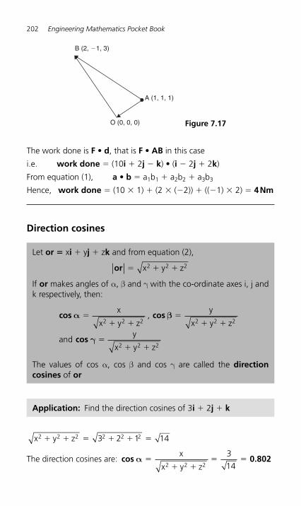
202 Engineering Mathematics Pocket Book
B (2, �1, 3)
A (1, 1, 1)
O (0, 0, 0) Figure 7.17
The work done is F • d , that is F • AB in this case
i.e. work done � (10 i � 2 j � k ) • ( i � 2 j � 2 k )
From equation (1), a • b � a 1 b 1 � a 2 b 2 � a 3 b 3
Hence, work done � (10 � 1) � (2 � ( � 2)) � (( � 1) � 2) � 4 Nm
Direction cosines
Let or � x i � y j � z k and from equation (2),
or � � �x y z2 2 2
If or makes angles of α, β and γ with the co-ordinate axes i, j and k respectively, then:
cos cos
cos
α β
γ
�� �
�� �
�� �
x
x y z
y
x y z
andy
x y z
2 2 2 2 2 2
2 2 2
,
The values of cos α, cos β and cos γ are called the direction cosines of or
Application: Find the direction cosines of 3 i � 2 j � k
x y z2 2 2 2 2 23 2 1 14� � � � � �
The direction cosines are: cos 0.802α �� �
�x
x y z2 2 2
3
14�
Vectors 203
cos 0.535β �� �
�y
x y z2 2 2
2
14�
and cos 0.267γ �� �
�y
x y z2 2 2
1
14�
7.8 Vector products
Let a � a 1 i � a 2 j � a 3 k and b � b 1 i � b 2 j � b 3 k
Vector or cross product: a b
i j k
a a a
b b b1 2 3
1 2 3
� � (4)
| |a b [(a a)(b b) (a b) ]2� � �• • • (5)
Application: Find (i) a � b and (ii) | |a b� for the vectors a � i � 4 j � 2 k and b � 2 i � j � 3 k
(i) From equation (4),
a b i j k
i j k
� �
i j k
1 4 2
2 1 3
4 2
1 3
1 2
2 3
1 4
2 1
12 2 3 4 1
�
�
��
�
�
�
� � � � � � �
� +
( ) ( ) ( 88)
� 10i 7j 9k� �
(ii) From equation (5) | |a b [(a a)(b b) (a b) ]2� � �• • •
Now a • a � (1)(1) � (4)(4) � ( � 2)( � 2) � 21
b • b � (2)(2) � (�1)(�1) � ( 3)( 3) � 14
and a • b � (1)(2) � (4)( � 1) � ( � 2)(3) � � 8
Thus, | |a b 15.17� � � � � �( )21 14 64 230
Application: Find (a) ( p � 2 q ) � r (b) p � (2 r � 3 q )if p � 4 i � j � 2 k , q � 3 i � 2 j � k and r � i � 2 k
204 Engineering Mathematics Pocket Book
(a) ( p � 2 q ) � r � [4 i � j � 2 k � 2(3 i � 2 j � k )] � ( i � 2 k )
� � � � � �
� � �
�
��
��
( ( )
i j k
from equation (4)
2 5 4 2
2 5 4
1 0 2
5 4
0 2
i j k) i k
i jj k
i j
� �
��
�
� � � � � � �
2 4
1 2
2 5
1 0
10 0 4 4 0 5( ) ( ) (k )
i.e. ( p � 2 q ) � r � � 10i � 8j � 5k
(b) (2 r � 3 q ) � (2 i � 4 k ) � (9 i � 6 j � 3 k )
� �
�
� � � � � � �
�
i j k
( ) ( ) ( )2 0 4
9 6 3
0 24 6 36 12 0i j k
24i 42j 12k� � �
Hence, p � (2 r � 3 q ) � (4 i � j � 2 k ) � ( � 24 i � 42 j � 12 k )
� �
� � �
� � � � � � � � �
�
i j k
( ) ( ) ( )
4 1 2
24 42 12
12 84 48 48 168 24i j k
96i 96j� � � 1144k 48(2i 2j 3k)or � � �
Application: Find the moment and the magnitude of the moment of a force of ( i � 2 j � 3 k) Newton’s about point B hav-ing co-ordinates (0, 1, 1), when the force acts on a line through A whose co-ordinates are (1, 3, 4)
The moment M about point B of a force vector F that has a position vector of r from A is given by:
M r F� �
r is the vector from B to A, i.e. r � BA But BA � BO � OA � OA � OBi.e. r � ( i � 3 j � 4 k ) � ( j � k ) � i � 2 j � 3 k
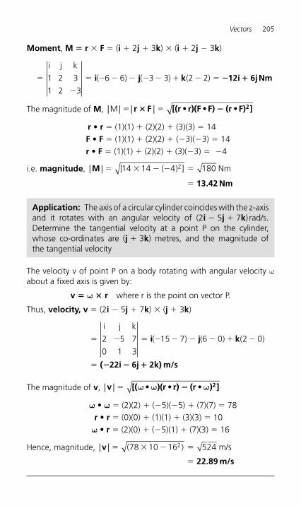
Vectors 205
Moment , M � r � F � ( i � 2 j � 3 k ) � ( i � 2 j � 3 k )
�
�
� � � � � � � � �
i j k
) ( ) )1 2 3
1 2 3
6 6 3 3 2 2i j k 12i 6jNm( ( � �
The magnitude of M , | | | |M � �r F [(r r)(F F) (r F) ]2� �• • •
r • r � (1)(1) � (2)(2) � (3)(3) � 14 F • F � (1)(1) � (2)(2) � ( � 3)( � 3) � 14 r • F � (1)(1) � (2)(2) � (3)( � 3) � � 4
i.e. magnitude , | |M � � � � �
�
[ ( ) ] Nm14 14 4 1802
13.42 Nm
Application: The axis of a circular cylinder coincides with the z-axis and it rotates with an angular velocity of (2 i � 5 j � 7 k ) rad/s. Determine the tangential velocity at a point P on the cylinder, whose co-ordinates are ( j � 3 k) metres, and the magnitude of the tangential velocity
The velocity v of point P on a body rotating with angular velocity ω about a fixed axis is given by:
v � ω � r where r is the point on vector P.
Thus, velocity, v � (2 i � 5 j � 7 k ) � ( j � 3 k )
� � � � � � � � �
�
i j k
( ) ( ) ( )2 5 7
0 1 3
15 7 6 0 2 0i j k
22i 6j 2k) m/s(� � �
The magnitude of v , | |v � [( )(r r) (r ) ]2ω ω ω• • •�
ω • ω � (2)(2) � ( � 5)( � 5) � (7)(7) � 78 r • r � (0)(0) � (1)(1) � (3)(3) � 10
ω • r � (2)(0) � ( � 5)(1) � (7)(3) � 16
Hence, magnitude, | | ( )v � � � �
�
78 10 16 5242 m/s
22.89 m/s
8 Complex Numbers
8.1 General formulae
z � a � jb � r(cos θ � j sin θ ) � r � θ � r e jθ where j 2 � � 1
Modulus, r | z | a b� � �( )2 2 Argument, θ � � �arg z tanba
1
Addition: (a � jb) � (c � jd) � (a � c) � j(b � d)
Subtraction: (a � jb) � (c � jd) � (a � c) � j(b � d)
Complex equations: If (m � jn) � (p � jq) then m � p and n � q
Multiplication: z 1 z 2 � r 1 r 2 � ( θ 1 � θ 2 )
Division: zz
rr
( )2 2
1 11 2� �∠ θ θ
De Moivre’s theorem: [r � θ ] n � rn � n θ � rn (cos n θ � j sin n θ )
8.2 Cartesian form
( � 1 � j2) and (3 – j4) are examples of Cartesian (or rectangular ) complex numbers. They are each of the form a � jb, ‘ a ’ being termed the real part and jb the imaginary part .
Application: Solve the quadratic equation 2x 2 � 3x � 5 � 0
Using the quadratic formula,
x[( ) ( )( )]
( )
( ) j
�� �
�� �
�� �
��
3 3 4 2 52 2
3 31
4
3 1 31
43 31
4
2
Hence, x34
j314
� � � or � 0.750 � j1.392, correct to 3 decimal places.
Complex Numbers 207
(2 � j3) � (3 � j4) � (�5 � j) � 2 � j3 � 3 � j4 � 5 � j � (2 � 3 � 5) � j(3 � 4 � 1) � 10 � j2
Application: Determine (2 � j3) � (3 � j4) � ( � 5 � j)
Application: Determine (3 � j2)(4 � j5)
(3 � j2)(4 � j5) � 12 � j15 � j8 � j 2 10 � (12 � � 10) � j(� 15 � 8) where j 2 � � 1 � 22 � j7
Application: Solve the complex equation:
(1 � j2)( � 2 � j3) � a � jb
(1 � j2)( � 2 � j3) � a � jb i.e. � 2 � j3 � j4 � j 2 6 � a � jb Hence, 4 � j7 � a � jb
Equating real and imaginary terms gives: a � 4 and b � � 7
Since (x � j2y) � (y � j3x) � 2 � j3
then (x � y) � j( � 2y � 3x) � 2 � j3
Equating real and imaginary parts gives: x y� � 2 (1)
and x y� � �3 2 3 (2)
Multiplying equation ( ) by gives: x y1 2 2 2 4� � (3)
Adding equations (2) and (3) gives: � x � 7 i.e. x � � 7
From equation (1), y � 9 , which may be checked in equation (2).
Application: Solve the equation (x � j2y) � (y � j3x) � 2 � j3
Application: Determine (3 � j4)(3 � j4)
(3 � j4)(3 � j4) � 9 � j12 � j12 � j 2 16 � 9 � 16 � 25
[(3 � j4) is called the complex conjugate of (3 � j4); whenever a complex number is multiplied by its conjugate, a real number results. In general, (a � jb)(a � jb) may be evaluated ‘ on sight ’ as a 2 � b 2 ]
208 Engineering Mathematics Pocket Book
2 53 4
2 53 4
3 43 4
6 8 15 203 4
14 232
2
2 2
�
��
�
��
�
��
� � �
�
�� �
jj
jj
( j )( j )
j j j
j55
��
� � �14
25j
2325
0.56 j0.92or
Application: Determine 2 53 4
�
�
jj
Application: If Z 1 � 1 � j3 and Z 2 � � 2 � j5 determine Z Z
Z Z1 2
1 2� in (a � jb) form
Z ZZ Z
1 2
1 2��
� � �
� � � ��
� � � �
� � �
(1 j3)( 2 j5)(1 j3) ( 2 j5)
j j jj
2 5 6 151 3 2
2
jj
j jj
jj
jj
jj
5
2 5 6 151 2
13 111 2
13 111 2
1 21 2
1
�� � � �
� ��
�
� �
��
� ��
� �
� �
�� 33 26 11 22
1 2
9 375
2
2 2
� � �
�
��
�
j j j
j
or95
j375
1.8 j7.4� �
Application: Show the following complex numbers on an Argand diagram (3 � j2), ( � 2 � j4), ( � 3 � j5) and (1 � j3)
In Figure 8.1 , the point A represents the complex number (3 � j2) and is obtained by plotting the co-ordinates (3, j2) as in graphical work. The Argand points B, C and D represent the complex numbers (� 2 � j4), ( � 3 � j5) and (1 � j3) respectively.
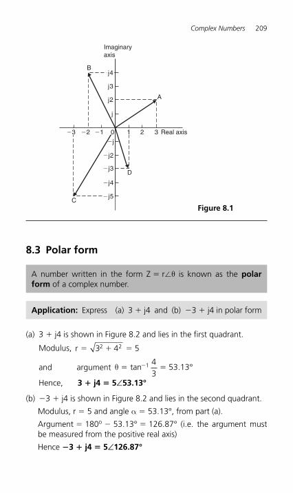
Complex Numbers 209
8.3 Polar form
�3 �2 �1 0 1 2 3 Real axis
�j2
�j3
�j4
Imaginaryaxis
j4
j3
j2
j
�j
�j5
A
B
C
D
Figure 8.1
A number written in the form Z � r � θ is known as the polarform of a complex number.
Application: Express (a) 3 � j4 and (b) �3 � j4 in polar form
(a) 3 � j4 is shown in Figure 8.2 and lies in the first quadrant.
Modulus, r � � �3 4 52 2
and argument θ � ��tan .1 43
53 13°
Hence, 3 � j4 � 5 ∠ 53.13°
(b) � 3 � j4 is shown in Figure 8.2 and lies in the second quadrant.
Modulus, r � 5 and angle α � 53.13°, from part (a).
Argument � 180 o � 53.13° � 126.87° (i.e. the argument must be measured from the positive real axis)
Hence � 3 � j4 � 5 ∠ 126.87°
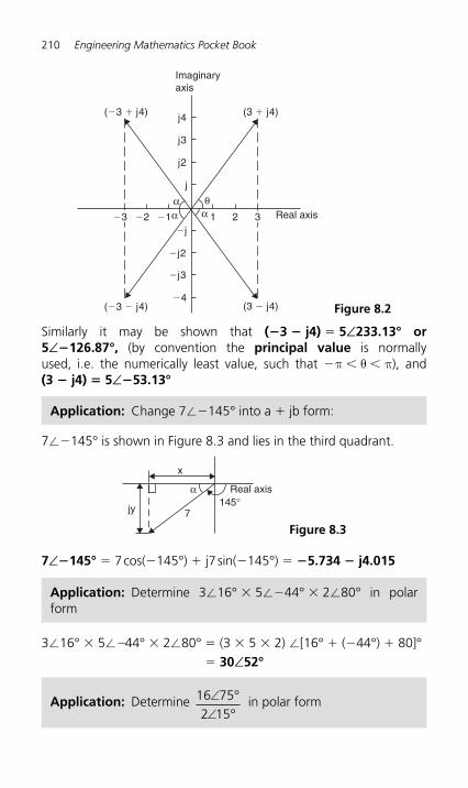
210 Engineering Mathematics Pocket Book
Similarly it may be shown that (� 3 � j4) � 5∠ 233.13° or5∠ � 126.87°, (by convention the principal value is normally used, i.e. the numerically least value, such that � π θ π), and (3 � j4) � 5∠ � 53.13°
Real axis
7145°
α
x
jy
Figure 8.3
1 2�1�2 3�3 Real axis
Imaginaryaxis
θαα
α
(�3 � j4)
(�3 � j4)
(3 � j4)
(3 � j4)
j4
�4
�j3
�j2
�j
j3
j2
j
Figure 8.2
Application: Change 7 � � 145° into a � jb form:
7 � � 145° is shown in Figure 8.3 and lies in the third quadrant.
Application: Determine 3 � 16° � 5 � � 44° � 2 �80° in polar form
3 � 16° � 5 � � 44° � 2 � 80° � (3 � 5 � 2) � [16° � ( � 44°) � 80]° � 30 ∠ 52°
Application: Determine 16 752 15
∠∠
°°
in polar form
7∠ � 145° � 7 cos( � 145 ° ) � j7 sin( � 145 ° ) � � 5.734 � j4.015
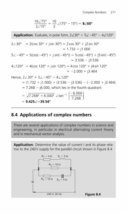
Complex Numbers 211
16 752 15
162
75 15∠∠
∠°
°° °� � �( ) 8 60∠ °
Application: Evaluate, in polar form, 2∠30° � 5∠ � 45° � 4∠120°
2 � 30° � 2(cos 30° � j sin 30°) � 2 cos 30° � j2 sin 30° � 1.732 � j1.000
5 � � 45° � 5(cos( � 45°) � j sin( � 45°)) � 5 cos( � 45°) � j5 sin( � 45°) � 3.536 � j3.536
4 � 120° � 4(cos 120° � j sin 120°) � 4 cos 120° � j4 sin 120° � � 2.000 � j3.464
Hence, 2 � 30° � 5 � � 45° � 4 � 120° � (1.732 � j1.000) � (3.536 � j3.536) � ( � 2.000 � j3.464) � 7.268 � j6.000, which lies in the fourth quadrant
� 7 268 6 0002 2. .� � tan � 1 �6 0007 268
..
⎛⎝⎜⎜⎜
⎞⎠⎟⎟⎟⎟
� 9.425 ∠ � 39.54°
8.4 Applications of complex numbers
There are several applications of complex numbers in science and engineering, in particular in electrical alternating current theory and in mechanical vector analysis.
Application: Determine the value of current I and its phase rela-tive to the 240 V supply for the parallel circuit shown in Figure 8.4
240 V, 50 Hz
R1 � 4 Ω
R2 � 10 Ω
R3 � 12 Ω XC � 5 Ω
XL � 3 Ω
l
Figure 8.4
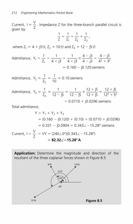
212 Engineering Mathematics Pocket Book
Current, IVZ
� . Impedance Z for the three-branch parallel circuit is given by:
1 1 1 1
4 3 10 12 5
1 2 3
1 2 3
Z Z Z Z,
where Z j , Z and Z j
� � �
� � � � �Ω Ω Ω
Admittance, YZ j j
jj
j
j
11
2 2
1 14 3
14 3
4 34 3
4 34 3
0 160 0 120
� ��
��
��
��
�
�
� �. . siemens
Admittance, YZ2
2
1 110
0 10� � � . siemens
Admittance, YZ j j
jj
j3
32 2
1 112 5
112 5
12 512 5
12 512 5
� ��
��
��
��
�
� � 0.0710 � j0.0296 siemens
Total admittance,
Y � Y 1 � Y 2 � Y 3
� (0.160 � j0.120) � (0.10) � (0.0710 � j0.0296)
� 0.331 � j0.0904 � 0.343 � � 15.28° siemens
Current, IVZ
� � VY � (240 � 0°)(0.343 � � 15.28°)
� 82.32∠ � 15.28°A
Application: Determine the magnitude and direction of the resultant of the three coplanar forces shown in Figure 8.5
45°
120°
210°
10 N8 N
15 N Figure 8.5
Complex Numbers 213
Force A, f A � 10 � 45° N, force B, f B � 8 � 120° N and force C, fC � 15 � 210° N
The resultant force � f A � f B � f C � 10� 45° � 8 � 120° � 15 � 210° � 10(cos 45 o � j sin 45 o ) � 8(cos 120 o � j sin 120 o )
� 15(cos 210 o � j sin 210 o ) � (7.071 � j7.071) � ( � 4.00 � j6.928) � ( � 12.99 � j7.50) � � 9.919 � j6.499
Magnitude of resultant force � � � �( )9 919 6 4992 2. . 11.86 N
Direction of resultant force ��
��tan 1 6 4999 919..
⎛⎝⎜⎜⎜
⎞⎠⎟⎟⎟⎟ 146.77°
(since � 9.919 � j6.499 lies in the second quadrant).
8.5 De Moivre’s theorem
De Moivre’s theorem states: [r∠ θ ] n � r n ∠ n θ
The theorem is used to determine powers and roots of complex numbers.
In general , when finding the n th root of a complex number, there are n solutions. For example, there are three solutions to a cube root, five solutions to a fifth root, and so on. In the solutions to the roots of a complex number, the modulus, r, is always the same, but the arguments, θ, are different. Arguments are symmet-rically spaced on an Argand diagram and are 360� n apart, where n is the number of the roots required. Thus if one of the solutions to the cube root of a complex number is, say, 5 �20°, the other two roots are symmetrically spaced 360 3� , i.e. 120° from this root, and the three roots are 5 �20°, 5 �140° and 5 �260°.
Application: Determine [3 � 20°] 4
[3 � 20°]4 � 3 4� (4 � 20°) � 81∠ 80° by de Moivre’s theorem.
214 Engineering Mathematics Pocket Book
Application: Determine (�2 � j3)6 in polar form
( � 2 � j3) � ( ) tan� ��
�2 332
2 2 1∠⎛
⎝⎜⎜⎜⎜
⎞
⎠⎟⎟⎟⎟⎟
� 13 �123.69° since � 2 � j3 lies in the second quadrant
( � 2 � j3) 6 � [ 13 � 123.69°] 6
� ( 13 ) 6� (6 � 123.69°) by De Moivre’s theorem
� 2197 � 742.14°
� 2197 � 382.14° (since 742.14 ° � 742.14° � 360° � 382.14°)
� 2197∠22.14° (since 382.14° � 382.14° � 360° � 22.14°)
Application: Determine the two square roots of the complex number (5 � j12) in polar and Cartesian forms
(5 � j12) � 5 12125
13 67 382 2 1� � ��∠ ∠tan⎛⎝⎜⎜⎜
⎞⎠⎟⎟⎟⎟ .
When determining square roots two solutions result. To obtain the second solution one way is to express 13 �67.38° also as 13� (67.38° � 360°), i.e. 13 �427.38°. When the angle is divided by 2 an angle less than 360° is obtained.
Hence 5 12 13 67 38 13 427 382 2� � ∠ ∠. .° and °
� [13 � 67.38°] 1 2/ and [13 � 427.38°] 1 2/
� 1312
67 38 1312
427 381 2 1 2/ /and ∠ ∠� � � �. .⎛⎝⎜⎜⎜
⎞⎠⎟⎟⎟⎟
⎛⎝⎜⎜⎜
⎞⎠⎟⎟⎟⎟
� 13 � 33.69° and 13 � 213.69°
� 3.61 � 33.69° and 3.61 � 213.69°
Thus, in polar form, the two roots are 3.61 ∠ 33.69° and3.61∠ � 146.31°
13 � 33.69° � 13 (cos 33.69° � j sin 33.69° ) � 3.0 � j2.0
13 �213.69° � 13 (cos 213.69° � j sin 213.69°) � � 3.0 � j2.0
Thus, in Cartesian form, the two roots are � (3.0 � j2.0)
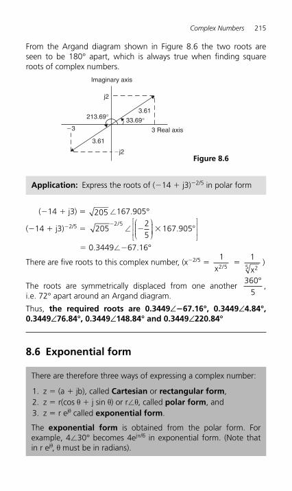
Complex Numbers 215
Imaginary axis
3.61
3.61
�3
�j2
j2
33.69°213.69°
3 Real axis
Figure 8.6
From the Argand diagram shown in Figure 8.6 the two roots are seen to be 180° apart, which is always true when finding square roots of complex numbers.
( � 14 � j3) � 205 � 167.905°
( � 14 � j3) � 2/5 � 20525
167 9052 5�
� � �/
∠⎛⎝⎜⎜⎜
⎞⎠⎟⎟⎟⎟
⎡
⎣⎢⎢
⎤
⎦⎥⎥.
� 0.3449 � � 67.16°
There are five roots to this complex number, (x � 2/5 � 12 5x /
� 1
25 x )
The roots are symmetrically displaced from one another 360
5°
, i.e. 72° apart around an Argand diagram.
Thus, the required roots are 0.3449 ∠ � 67.16°, 0.3449 ∠ 4.84°, 0.3449∠ 76.84°, 0.3449∠ 148.84° and 0.3449∠ 220.84°
8.6 Exponential form
Application: Express the roots of ( � 14 � j3) � 2/5 in polar form
There are therefore three ways of expressing a complex number:
1. z � (a � jb), called Cartesian or rectangular form , 2. z � r(cos θ � j sin θ ) or r � θ , called polar form , and 3. z � r e jθ called exponential form .
The exponential form is obtained from the polar form. For example, 4 �30° becomes 4e jπ /6 in exponential form. (Note that in r e jθ , θ must be in radians).
216 Engineering Mathematics Pocket Book
(3 � j4) � 5∠ � 53.13 ° � 5∠ � 0.927 in polar form � 5e � j0.927 in exponential form
Application: Express (3 � j4) in polar and exponential forms
Application: Express 7.2e j1.5 in rectangular form
7.2e j1.5 � 7.2 � 1.5 rad ( � 7.2 � 85.944°) in polar form � 7.2 cos 1.5 � j7.2 sin 1.5 � (0.509 � j7.182) in rectangular form
Application: If z � 2e 1 � j π /3 express z in Cartesian form
z � 2e 1� j π /3 � (2e 1 )(e jπ /3 ) by the laws of indices
� (2e 1 ) � π3
(or 2e � 60°) in polar form
� 2e cos sinπ π3 3
� j⎛⎝⎜⎜⎜
⎞⎠⎟⎟⎟⎟ � (2.718 � j4.708) in Cartesian
form
Application: If z � 4e j1.3 find ln z in polar form
If z � 4e j1.3 then ln z � ln(4e j1.3 )
� ln 4 � j1.3 (or 1.386 � j1.300 ) in Cartesianform (by the laws of logarithms)
� 1.90∠ 43.17° or 1.90∠ 0.753 in polar form.
Application: Determine ln(3 � j4)
ln(3 � j4) � ln [5 � 0.927] � ln[5e j0.927 ] � ln 5 � ln(e j0.927 )
� ln 5 � j0.927 � 1.609 � j0.927
� 1.857∠ 29.95° or 1.857 ∠ 0.523
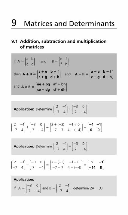
9 Matrices and Determinants
9.1 Addition, subtraction and multiplication of matrices
If Aa b
c dand B
e f
f h� �
⎛
⎝⎜⎜⎜⎜
⎞
⎠⎟⎟⎟⎟
⎛
⎝⎜⎜⎜⎜
⎞
⎠⎟⎟⎟⎟
then A Ba e b f
c g d h� �
� �
� �
⎛
⎝⎜⎜⎜⎜
⎞
⎠⎟⎟⎟⎟
and A Ba e b f
c g d h� �
� �
� �
⎛
⎝⎜⎜⎜⎜
⎞
⎠⎟⎟⎟⎟
and A Bae bg af bh
ce dg cf dh� �
� �
� �
⎛
⎝⎜⎜⎜⎜
⎞
⎠⎟⎟⎟⎟
Application: Determine 2 1
7 4
3 0
7 4
�
��
�
�
⎛
⎝⎜⎜⎜⎜
⎞
⎠⎟⎟⎟⎟
⎛
⎝⎜⎜⎜⎜
⎞
⎠⎟⎟⎟⎟
2 1
7 4
3 0
7 4
2 3 1 0
7 7 4 4
�
��
�
��
� � �
� �
⎛
⎝⎜⎜⎜⎜
⎞
⎠⎟⎟⎟⎟
⎛
⎝⎜⎜⎜⎜
⎞
⎠⎟⎟⎟⎟
++ +( )
( )
⎛⎛
⎝⎜⎜⎜⎜
⎞
⎠⎟⎟⎟⎟
⎛
⎝⎜⎜⎜⎜
⎞
⎠⎟⎟⎟⎟
�� �1 1
0 0
Application: Determine 2 1
7 4
3 0
7 4
�
��
�
�
⎛
⎝⎜⎜⎜⎜
⎞
⎠⎟⎟⎟⎟
⎛
⎝⎜⎜⎜⎜
⎞
⎠⎟⎟⎟⎟
2 1
7 4
3 0
7 4
2 3 1 0
7 7 4 4
�
��
�
��
� � � �
� � � �
⎛
⎝⎜⎜⎜⎜
⎞
⎠⎟⎟⎟⎟
⎛
⎝⎜⎜⎜⎜
⎞
⎠⎟⎟⎟⎟
( )
( )
⎛⎛
⎝⎜⎜⎜⎜
⎞
⎠⎟⎟⎟⎟
⎛
⎝⎜⎜⎜⎜
⎞
⎠⎟⎟⎟⎟
�5 1
14 8
�
�
Application:
If A and B determine A B��
��
�
��
3 0
7 4
2 1
7 42 3
⎛
⎝⎜⎜⎜⎜
⎞
⎠⎟⎟⎟⎟
⎛
⎝⎜⎜⎜⎜
⎞
⎠⎟⎟⎟⎟
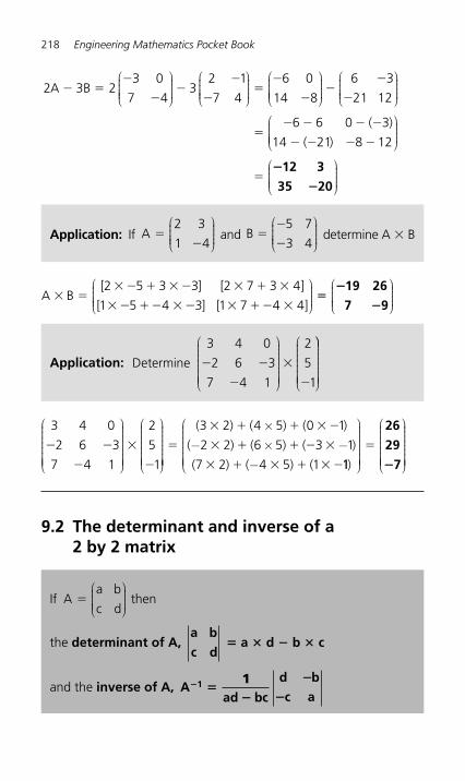
218 Engineering Mathematics Pocket Book
2 23 0
7 43
2 1
7 4
6 0
14 8A 3B� �
�
��
�
��
�
�
⎛
⎝⎜⎜⎜⎜
⎞
⎠⎟⎟⎟⎟
⎛
⎝⎜⎜⎜⎜
⎞
⎠⎟⎟⎟⎟
⎛
⎝⎜⎜⎜⎜⎜
⎞
⎠⎟⎟⎟⎟
⎛
⎝⎜⎜⎜⎜
⎞
⎠⎟⎟⎟⎟
⎛
⎝⎜⎜⎜
��
�
�� � � �
� � � �
6 3
21 12
6 6 0 3
14 21 8 12
( )
( )⎜⎜
⎞
⎠⎟⎟⎟⎟
⎛
⎝⎜⎜⎜⎜
⎞
⎠⎟⎟⎟⎟
��
�
12 3
35 20
Application: If A ��
2 3
1 4
⎛
⎝⎜⎜⎜⎜
⎞
⎠⎟⎟⎟⎟ and B �
�
�
5 7
3 4
⎛
⎝⎜⎜⎜⎜
⎞
⎠⎟⎟⎟⎟ determine A � B
A B� �� � � � � � � �
� � �� � � � �� �
[ ] [ ]
[ ] [ ]
2 5 3 3 2 7 3 4
1 5 4 3 1 7 4 4
⎛
⎝⎜⎜⎜⎜
⎞
⎠⎟⎟⎟⎟
���
�
19 26
7 9
⎛
⎝⎜⎜⎜⎜
⎞
⎠⎟⎟⎟⎟
Application: Determine
3 4 0
2 6 3
7 4 1
2
5
1
� �
�
�
�
⎛
⎝
⎜⎜⎜⎜⎜⎜⎜⎜
⎞
⎠
⎟⎟⎟⎟⎟⎟⎟⎟⎟
⎛
⎝
⎜⎜⎜⎜⎜⎜⎜⎜
⎞⎞
⎠
⎟⎟⎟⎟⎟⎟⎟⎟⎟
3 4 0
2 6 3
7 4 1
2
5
1
� �
�
�
�
⎛
⎝
⎜⎜⎜⎜⎜⎜⎜⎜
⎞
⎠
⎟⎟⎟⎟⎟⎟⎟⎟⎟
⎛
⎝
⎜⎜⎜⎜⎜⎜⎜⎜
⎞
⎠
⎟⎟⎟⎟⎟⎟⎟⎟⎟⎟
×− × −
−�
� � � � �
� � � � �
� � � � � �
( ) ( ) ( )
( ) ( ) ( )
( ) ( ) (
3 2 4 5 0 1
2 2 6 5 3 1
7 2 4 5 1 11)
⎛
⎝
⎜⎜⎜⎜⎜⎜⎜⎜
⎞
⎠
⎟⎟⎟⎟⎟⎟⎟⎟⎟
⎛
⎝
⎜⎜⎜⎜⎜⎜⎜⎜
⎞
⎠
⎟⎟⎟⎟⎟⎟⎟⎟⎟�
26
29
7�
9.2 The determinant and inverse of a 2 by 2 matrix
If Aa b
c dthen�
⎛
⎝⎜⎜⎜⎜
⎞
⎠⎟⎟⎟⎟
the determinant of A,a b
c d � a � d � b � c
and the inverse of A , Aad bc
d b
c a1� �
�
�
�
1
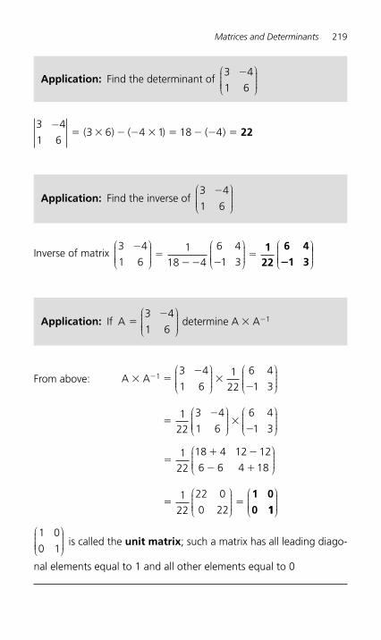
Matrices and Determinants 219
3 4
1 63 6 4 1 18 4
−� � � � � � � � �( ) ( ) ( ) 22
Application : Find the determinant of 3 4
1 6
�⎛
⎝⎜⎜⎜⎜
⎞
⎠⎟⎟⎟⎟
Application: Find the inverse of 3 4
1 6
�⎛
⎝⎜⎜⎜⎜
⎞
⎠⎟⎟⎟⎟
Inverse of matrix 3 4
1 61
18 4
6 4
1 3
��
� � ��
⎛
⎝⎜⎜⎜⎜
⎞
⎠⎟⎟⎟⎟
⎛
⎝⎜⎜⎜⎜
⎞
⎠⎟⎟⎟⎟
⎛
⎝⎜⎜⎜⎜
⎞
⎠1
22
6 4
1 3�⎟⎟⎟⎟⎟
Application: If A determine A A��
� �3 4
1 61
⎛
⎝⎜⎜⎜⎜
⎞
⎠⎟⎟⎟⎟
From above: A A 1� ��
��
��
�3 4
1 61
22
6 4
1 3
122
3 4
1 6
⎛
⎝⎜⎜⎜⎜
⎞
⎠⎟⎟⎟⎟
⎛
⎝⎜⎜⎜⎜
⎞
⎠⎟⎟⎟⎟
⎛
⎝⎜⎜⎜⎜⎜
⎞
⎠⎟⎟⎟⎟
⎛
⎝⎜⎜⎜⎜
⎞
⎠⎟⎟⎟⎟
��
6 4
1 3
�� �
� �
� �
122
18 4 12 12
6 6 4 18
122
22 0
0 22
⎛
⎝⎜⎜⎜⎜
⎞
⎠⎟⎟⎟⎟
⎛
⎝⎜⎜⎜⎜
⎞
⎠⎟⎟⎟⎟
1 0
0 11
⎛
⎝⎜⎜⎜⎜
⎞
⎠⎟⎟⎟⎟
1 0
0 1
⎛
⎝⎜⎜⎜⎜
⎞
⎠⎟⎟⎟⎟ is called the unit matrix; such a matrix has all leading diago-
nal elements equal to 1 and all other elements equal to 0
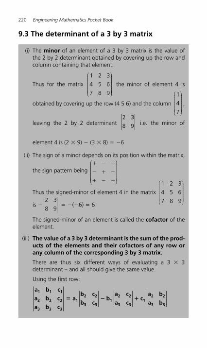
220 Engineering Mathematics Pocket Book
9.3 The determinant of a 3 by 3 matrix
(i) The minor of an element of a 3 by 3 matrix is the value of the 2 by 2 determinant obtained by covering up the row and column containing that element.
Thus for the matrix
1 2 3
4 5 6
7 8 9
⎛
⎝
⎜⎜⎜⎜⎜⎜⎜⎜
⎞
⎠
⎟⎟⎟⎟⎟⎟⎟⎟⎟ the minor of element 4 is
obtained by covering up the row (4 5 6) and the column
1
4
7
⎛
⎝
⎜⎜⎜⎜⎜⎜⎜⎜
⎞
⎠
⎟⎟⎟⎟⎟⎟⎟⎟⎟ ,
leaving the 2 by 2 determinant2 3
8 9 i.e. the minor of
element 4 is (2 � 9) � (3 � 8) � � 6
(ii) The sign of a minor depends on its position within the matrix,
the sign pattern being � � �
� � �
� � �
⎛
⎝
⎜⎜⎜⎜⎜⎜⎜⎜
⎞
⎠
⎟⎟⎟⎟⎟⎟⎟⎟⎟
Thus the signed-minor of element 4 in the matrix
1 2 3
4 5 6
7 8 9
⎛
⎝
⎜⎜⎜⎜⎜⎜⎜⎜
⎞
⎠
⎟⎟⎟⎟⎟⎟⎟⎟⎟
is �2 3
8 9 � � ( � 6) � 6
The signed-minor of an element is called the cofactor of the element.
(iii) The value of a 3 by 3 determinant is the sum of the prod-ucts of the elements and their cofactors of any row or any column of the corresponding 3 by 3 matrix.
There are thus six different ways of evaluating a 3 � 3 d eterminant – and all should give the same value.
Using the first row:
a b c
a b c
a b c
ab c
b cb
a c
a cc
a b
a b
1 1 1
2 2 2
3 3 3
12 2
3 31
2 2
3 31
2 2
3 3� � �
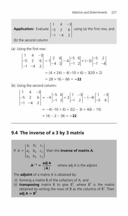
Matrices and Determinants 221
(a) Using the first row:
1 4 3
5 2 6
1 4 2
12 6
4 24
5 6
1 23
5 2
1 4
�
�
� �
��
��
�� �
�
� �( )
� � � � � � �
� � � �
( ) ( ) ( )4 24 4 10 6 3 20 2
28 16 66 �22 (b) Using the second column:
1 4 3
5 2 6
1 4 2
45 6
1 22
1 3
1 24
1 3
5 6
�
�
� �
� ��
��
�
�� �
�
�( )
� � � � � � � �
� � � �
4 10 6 2 2 3 4 6 15
16 2 36
( ) ( ) ( )
�22
9.4 The inverse of a 3 by 3 matrix
Application: Evaluate 1 4 3
5 2 6
1 4 2
�
�
� �
using (a) the first row, and
(b) the second column
If A
a b c
a b c
a b c
�
1 1 1
2 2 2
3 3 3
⎛
⎝
⎜⎜⎜⎜⎜⎜⎜⎜
⎞
⎠
⎟⎟⎟⎟⎟⎟⎟⎟⎟ then the inverse of matrix A ,
Aadj A
A1� �
| |where adj A is the adjoint
The adjoint of a matrix A is obtained by:
(i) forming a matrix B of the cofactors of A, and (ii) transposing matrix B to give B T, where B T is the matrix
obtained by writing the rows of B as the columns of B T. Then adj A � B T
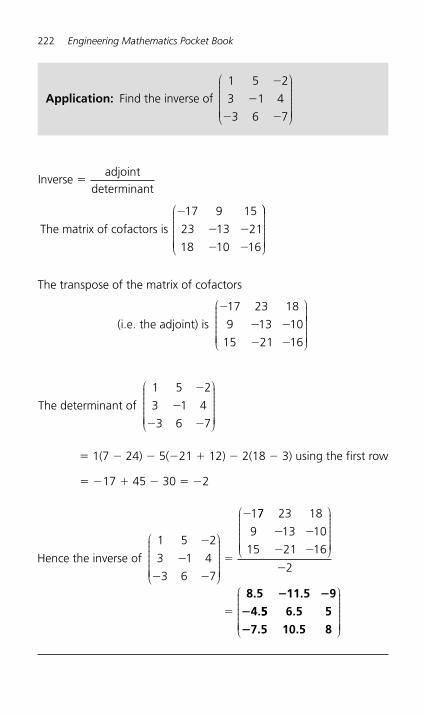
222 Engineering Mathematics Pocket Book
Inverseint
determinant�
adjo
The matrix of cofactors is
�
� �
� �
17 9 15
23 13 21
18 10 16
⎛
⎝
⎜⎜⎜⎜⎜⎜⎜⎜
⎞⎞
⎠
⎟⎟⎟⎟⎟⎟⎟⎟⎟
The transpose of the matrix of cofactors
(i.e. the adjoint) is
�
� �
� �
17 23 18
9 13 10
15 21 16
⎛
⎝
⎜⎜⎜⎜⎜⎜⎜⎜
⎞
⎠
⎟⎟⎟⎟⎟⎟⎟⎟⎟⎟
The determinant of
1 5 2
3 1 4
3 6 7
�
�
� �
⎛
⎝
⎜⎜⎜⎜⎜⎜⎜⎜
⎞
⎠
⎟⎟⎟⎟⎟⎟⎟⎟⎟
� 1(7 � 24) � 5( � 21 � 12) � 2(18 � 3) using the first row
� � 17 � 45 � 30 � � 2
Hence the inverse of
1 5 2
3 1 4
3 6 7
1
�
�
� �
�
�
⎛
⎝
⎜⎜⎜⎜⎜⎜⎜⎜
⎞
⎠
⎟⎟⎟⎟⎟⎟⎟⎟⎟
77 23 18
9 13 10
15 21 16
2
� �
� �
�
�
⎛
⎝
⎜⎜⎜⎜⎜⎜⎜⎜
⎞
⎠
⎟⎟⎟⎟⎟⎟⎟⎟⎟
8.5 11.5 9
4.
� �
� 55 6.5 5
7.5 10.5 8�
⎛
⎝
⎜⎜⎜⎜⎜⎜⎜⎜
⎞
⎠
⎟⎟⎟⎟⎟⎟⎟⎟⎟
Application: Find the inverse of
1 5 2
3 1 4
3 6 7
�
�
� �
⎛
⎝
⎜⎜⎜⎜⎜⎜⎜⎜
⎞
⎠
⎟⎟⎟⎟⎟⎟⎟⎟⎟
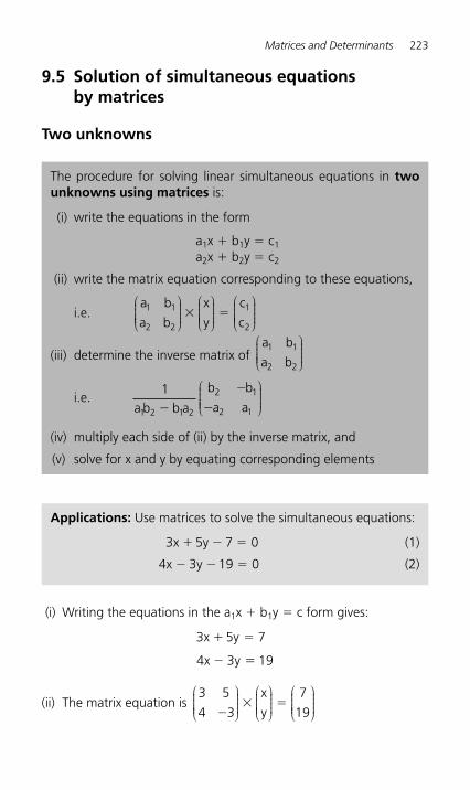
Matrices and Determinants 223
9.5 Solution of simultaneous equations by matrices
Two unknowns
The procedure for solving linear simultaneous equations in twounknowns using matrices is:
(i) write the equations in the form
a 1 x � b 1 y � c 1 a 2 x � b 2 y � c 2
(ii) write the matrix equation corresponding to these equations,
i.e.
a b
a b
x
y
c
c1 1
2 2
1
2
⎛
⎝⎜⎜⎜⎜
⎞
⎠⎟⎟⎟⎟
⎛
⎝⎜⎜⎜⎜
⎞
⎠⎟⎟⎟⎟
⎛
⎝⎜⎜⎜⎜
⎞
⎠⎟⎟⎟⎟
� �
(iii) determine the inverse matrix of a b
a b1
2
1
2
⎛
⎝⎜⎜⎜⎜
⎞
⎠⎟⎟⎟⎟
i.e.1
a b b a
b b
a a2
1 2 1 2
1
2 1�
�
�
⎛
⎝⎜⎜⎜⎜
⎞
⎠⎟⎟⎟⎟
(iv) multiply each side of (ii) by the inverse matrix, and
(v) solve for x and y by equating corresponding elements
Applications: Use matrices to solve the simultaneous equations:
3x y 7 0� � �5 (1)
4x 3y 9 0� � �1 (2)
(i) Writing the equations in the a 1 x � b 1 y � c form gives:
3x y 7
4x 3y 9
� �
� �
5
1
(ii) The matrix equation is 3 5
4 3
7
19�� �
⎛
⎝⎜⎜⎜⎜
⎞
⎠⎟⎟⎟⎟
⎛
⎝⎜⎜⎜⎜
⎞
⎠⎟⎟⎟⎟
⎛
⎝⎜⎜⎜⎜
⎞
⎠⎟⎟⎟⎟
x
y
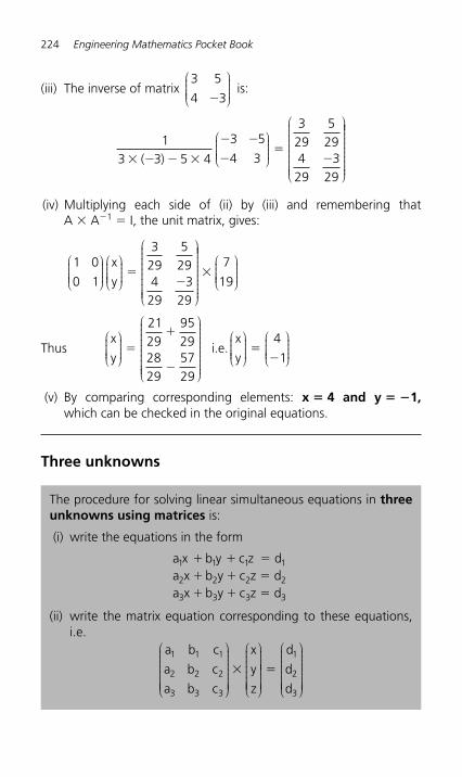
224 Engineering Mathematics Pocket Book
(iii) The inverse of matrix 3 5
4 3�
⎛
⎝⎜⎜⎜⎜
⎞
⎠⎟⎟⎟⎟
is:
13 3 5 4
3 5
4 3
329
529
429
329
� � � �
� �
��
�( )
⎛
⎝⎜⎜⎜⎜
⎞
⎠⎟⎟⎟⎟
⎛
⎝
⎜⎜⎜⎜⎜⎜⎜⎜⎜⎜
⎞
⎠
⎟⎟⎟⎟⎟⎟⎟⎟⎟⎟⎟⎟
(iv) Multiplying each side of (ii) by (iii) and remembering that A � A � 1 � I, the unit matrix, gives:
1 0
0 1
329
529
429
329
⎛
⎝⎜⎜⎜⎜
⎞
⎠⎟⎟⎟⎟⎛
⎝⎜⎜⎜⎜
⎞
⎠⎟⎟⎟⎟
⎛
⎝
⎜⎜⎜⎜⎜⎜⎜⎜⎜⎜
⎞
⎠
x
y�
�
⎟⎟⎟⎟⎟⎟⎟⎟⎟⎟⎟⎟
⎛
⎝⎜⎜⎜⎜
⎞
⎠⎟⎟⎟⎟
�7
19
Thus x
y
⎛
⎝⎜⎜⎜⎜
⎞
⎠⎟⎟⎟⎟
−
⎛
⎝
⎜⎜⎜⎜⎜⎜⎜⎜⎜⎜
⎞
⎠
⎟⎟⎟⎟⎟⎟⎟⎟⎟⎟⎟
�
�2129
9529
2829
5729
i.e.x
y
⎛
⎝⎜⎜⎜⎜
⎞
⎠⎟⎟⎟⎟
⎛
⎝⎜⎜⎜⎜
⎞
⎠⎟⎟⎟⎟
��
4
1
(v) By comparing corresponding elements: x � 4 and y � � 1,
which can be checked in the original equations.
Three unknowns
The procedure for solving linear simultaneous equations in three unknowns using matrices is:
(i) write the equations in the form
a x b y c z da x b y c z da x b y c z d
1 1 1 1
2 2 2 2
3 3 3 3
� � �
� � �
� � � (ii) write the matrix equation corresponding to these equations,
i.e. a b c
a b c
a b c
x
y
z
1 1 1
2 2 2
3 3 3
⎛
⎝
⎜⎜⎜⎜⎜⎜⎜⎜
⎞
⎠
⎟⎟⎟⎟⎟⎟⎟⎟⎟
⎛
⎝
⎜⎜⎜⎜⎜⎜⎜⎜
⎞
⎠
⎟⎟⎟� ⎟⎟⎟⎟⎟⎟⎟
⎛
⎝
⎜⎜⎜⎜⎜⎜⎜⎜
⎞
⎠
⎟⎟⎟⎟⎟⎟⎟⎟⎟�
d
d
d
1
2
3
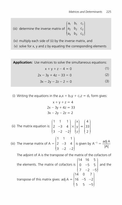
Matrices and Determinants 225
(i) Writing the equations in the a 1 x � b 1 y � c 1 z � d 1 form gives:
x y z
x y z
x y z
� � �
� � �
� � �
4
2 3 4 33
3 2 2 2
(ii) The matrix equation is: 1 1 1
2 3 4
3 2 2
�
� �
�
⎛
⎝
⎜⎜⎜⎜⎜⎜⎜⎜
⎞
⎠
⎟⎟⎟⎟⎟⎟⎟⎟⎟
⎛
⎝
⎜⎜⎜⎜⎜⎜⎜⎜
⎞
⎠
⎟⎟⎟⎟⎟⎟⎟⎟⎟
x
y
z
��
4
33
2
⎛
⎝
⎜⎜⎜⎜⎜⎜⎜⎜
⎞
⎠
⎟⎟⎟⎟⎟⎟⎟⎟⎟
(iii) The inverse matrix of A �
1 1 1
2 3 4
3 2 2
−− −
⎛
⎝
⎜⎜⎜⎜⎜⎜⎜⎜
⎞
⎠
⎟⎟⎟⎟⎟⎟⎟⎟⎟ is given by A� �1 adj A
A| |
The adjoint of A is the transpose of the matrix of the cofactors of
the elements. The matrix of cofactors is 14 16 5
0 5 5
7 2 5
�
� �
⎛
⎝
⎜⎜⎜⎜⎜⎜⎜⎜
⎞
⎠
⎟⎟⎟⎟⎟⎟⎟⎟⎟ and the
transpose of this matrix gives: adj A � � �
�
14 0 7
16 5 2
5 5 5
⎛
⎝
⎜⎜⎜⎜⎜⎜⎜⎜
⎞
⎠
⎟⎟⎟⎟⎟⎟⎟⎟⎟
(iii) determine the inverse matrix of
a b c
a b c
a b c
1 1 1
2 2 2
3 3 3
⎛
⎝
⎜⎜⎜⎜⎜⎜⎜⎜
⎞
⎠
⎟⎟⎟⎟⎟⎟⎟⎟⎟
(iv) multiply each side of (ii) by the inverse matrix, and
(v) solve for x, y and z by equating the corresponding elements
Application: Use matrices to solve the simultaneous equations:
x y z 0� � � �4 (1)
2 3 4 33 0x y z� � � � (2)
3 2 2 0x y z 2� � � � (3)
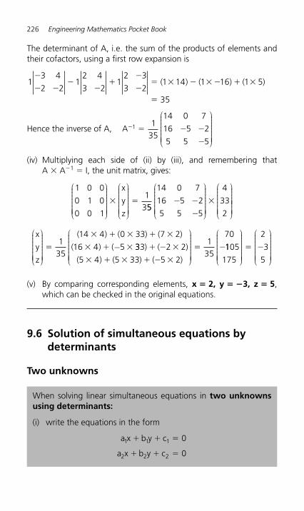
226 Engineering Mathematics Pocket Book
The determinant of A, i.e. the sum of the products of elements and their cofactors, using a first row expansion is
13 4
2 21
2 4
3 21
2 3
3 21 14 1 16 1 5
35
�
� ��
��
�
�� � � � � � �
�
( ) ( ) ( )
Hence the inverse of A, A� � � �
�
1 135
14 0 7
16 5 2
5 5 5
⎛
⎝
⎜⎜⎜⎜⎜⎜⎜⎜
⎞
⎠
⎟⎟⎟⎟⎟⎟⎟⎟⎟
(iv) Multiplying each side of (ii) by (iii), and remembering that A � A � 1 � I, the unit matrix, gives:
1 0 0
0 1 0
0 0 1
13
⎛
⎝
⎜⎜⎜⎜⎜⎜⎜⎜
⎞
⎠
⎟⎟⎟⎟⎟⎟⎟⎟⎟
⎛
⎝
⎜⎜⎜⎜⎜⎜⎜⎜
⎞
⎠
⎟⎟⎟⎟⎟⎟⎟⎟⎟� �
x
y
z55
14 0 7
16 5 2
5 5 5
4
33
2
� �
�
�
⎛
⎝
⎜⎜⎜⎜⎜⎜⎜⎜
⎞
⎠
⎟⎟⎟⎟⎟⎟⎟⎟⎟
⎛
⎝
⎜⎜⎜⎜⎜⎜⎜⎜
⎞
⎠
⎟⎟⎟⎟⎟⎟⎟⎟⎟⎟
x
y
z
⎛
⎝
⎜⎜⎜⎜⎜⎜⎜⎜
⎞
⎠
⎟⎟⎟⎟⎟⎟⎟⎟⎟−�
� � � � �
� � �1
35
14 4 0 33 7 2
16 4 5
( ) ( ) ( )
( ) ( 333 2 2
5 4 5 33 5 2
135
70
) ( )
( ) ( ) ( )
� � �
� � � � � �
� �
⎛
⎝
⎜⎜⎜⎜⎜⎜⎜⎜
⎞
⎠
⎟⎟⎟⎟⎟⎟⎟⎟⎟1105
175
2
3
5
⎛
⎝
⎜⎜⎜⎜⎜⎜⎜⎜
⎞
⎠
⎟⎟⎟⎟⎟⎟⎟⎟⎟
⎛
⎝
⎜⎜⎜⎜⎜⎜⎜⎜
⎞
⎠
⎟⎟⎟⎟⎟⎟⎟⎟⎟� �
(v) By comparing corresponding elements, x � 2, y � �3, z � 5 , which can be checked in the original equations.
9.6 Solution of simultaneous equations by determinants
Two unknowns
When solving linear simultaneous equations in two unknowns using determinants:
(i) write the equations in the form
a x b y c
a x b y c
1 1 1
2 2 2
0
0
� � �
� � �
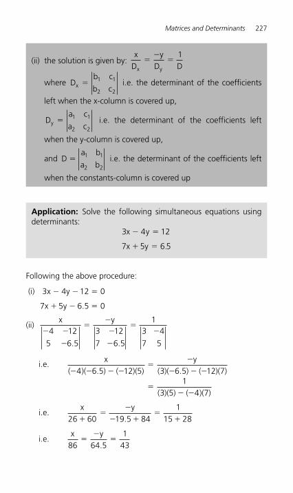
Matrices and Determinants 227
Following the above procedure:
(i) 3x 4y 12 0
7x 5y 6.5 0
� � �
� � �
(ii)
x y� �
�
��
�
�
��4 12
5 6 5
3 12
7 6 5
13 4
7 5. .
i.e.x y
( )( . ) ( )( ) ( )( . ) ( )( )
( )( ) ( )( )
� � � ��
�
� � �
�� �
4 6 5 12 5 3 6 5 12 71
3 5 4 7
i.e. x y
26 60 19 5 841
15 28��
�
� ��
�.
i.e.x y
86 64 51
43�
��
.
(ii) the solution is given by: x
Dy
D1Dx y
��
�
where Db c
b cx1 1
2 2� i.e. the determinant of the coefficients
left when the x-column is covered up,
Da c
a cy1 1
2 2� i.e. the determinant of the coefficients left
when the y-column is covered up,
and Da b
a b�
1 1
2 2 i.e. the determinant of the coefficients left
when the constants-column is covered up
Application: Solve the following simultaneous equations using determinants:
3 4 12
7 5 6 5
x y
x y .
� �
� �
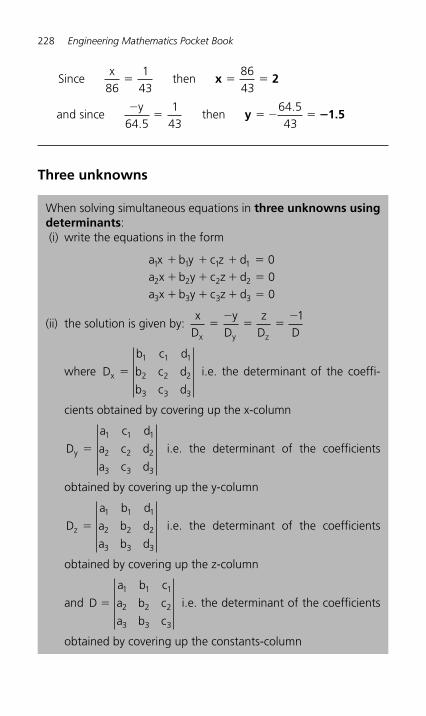
228 Engineering Mathematics Pocket Book
Since then
x86
143
8643
� � �x 2
and since then
�� � � �
y64 5
143.
y 1.564.543
�
Three unknowns
When solving simultaneous equations in three unknowns using determinants : (i) write the equations in the form
a x b y c z da x b y c z da x b y c z d
1 1 1 1
2 2 2 2
3 3 3 3
000
� � � �
� � � �
� � � �
(ii) the solution is given by: x
Dy
Dz
D1
Dx y z
��
� ��
where D
b c d
b c d
b c dx
1 1 1
2 2 2
3 3 3
� i.e. the determinant of the coeffi-
cients obtained by covering up the x-column
D
a c d
a c d
a c dy
1 1 1
2 2 2
3 3 3
� i.e. the determinant of the coefficients
obtained by covering up the y-column
D
a b d
a b d
a b dz
1 1 1
2 2 2
3 3 3
� i.e. the determinant of the coefficients
obtained by covering up the z-column
and D
a b c
a b c
a b c
1 1
2 2 2
3 3 3
�
1
i.e. the determinant of the coefficients
obtained by covering up the constants-column
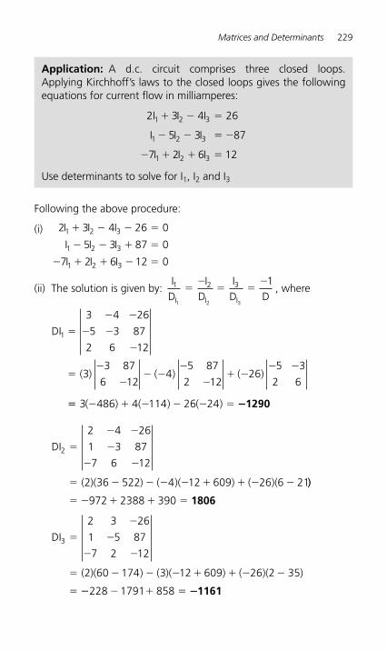
Matrices and Determinants 229
Following the above procedure:
(i)
2 3 4 26 0
5 3 87 0
7 2 6 12 0
1 2 3
1 2 3
1 2 3
I I I
I I I
I I I
� � � �
� � � �
� � � � �
(ii) The solution is given by: I
DI
DID DI I
1 2 3
1 2 3
1�
�� �
�
I
, where
DI
( ) ( ) ( )
1
3 4 26
5 3 87
2 6 12
33 87
6 124
5 87
2 1226
5 3
2 6
�
� �
� �
�
��
�� �
�
�� �
� �
�� � � � � � �3 486 4 114 26 24( ) ( ) ( ) �1290
DI
( )( ) ( )( ) ( )(
2
2 4 26
1 3 87
7 6 12
2 36 522 4 12 609 26 6 21
�
� �
�
� �
� � � � � � � � � ))
� � � � �972 2388 390 1806
DI
( )( ) ( )( ) ( )( )
3
2 3 26
1 5 87
7 2 12
2 60 174 3 12 609 26 2 35
�
�
�
� �
� � � � � � � �
� �� � � �228 1791 858 �1161
Application: A d.c. circuit comprises three closed loops. Applying Kirchhoff’s laws to the closed loops gives the following equations for current flow in milliamperes:
2I I I
I I I
I I I
1 2 3
1 2 3
1 2 3
3 4 26
5 3 87
7 2 6 12
� � �
� � � �
� � � � Use determinants to solve for I 1 , I 2 and I 3
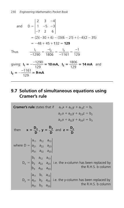
230 Engineering Mathematics Pocket Book
and D
( )( ) ( )( ) ( )( )
�
�
� �
�
� � � � � � � �
� � � �
2 3 4
1 5 3
7 2 6
2 30 6 3 6 21 4 2 35
48 45 1132 � 129
Thus
I I I1 2 3
1290 1806 11611
129��
��
��
�
giving: andI 10 mA, I 14 mA
I
1 2
3
� � � �
� �
��
��
1290129
1806129
1161129
99 mA
9.7 Solution of simultaneous equations using Cramer’s rule
Cramer’s rule states that if a x a y a z b
a x a y a z b
a x a y a z b
11 12 13 1
21 22 23 2
31 32 33 3
� � �
� � �
� � �
then and x
DD
, yD
Dz
DD
x y z� � �
where D
a a a
a a a
a a a
11 12
21 22 23
31 32 33
�
13
D
b a a
b a a
b a ax
12 13
2 22 23
3 32 33
�
1
i.e. the x-column has been replaced by the R.H.S. b column
D
a b a
a b a
a b ay
11 1 13
21 2 23
31 3 33
� i.e. the y-column has been replaced by the R.H.S. b column
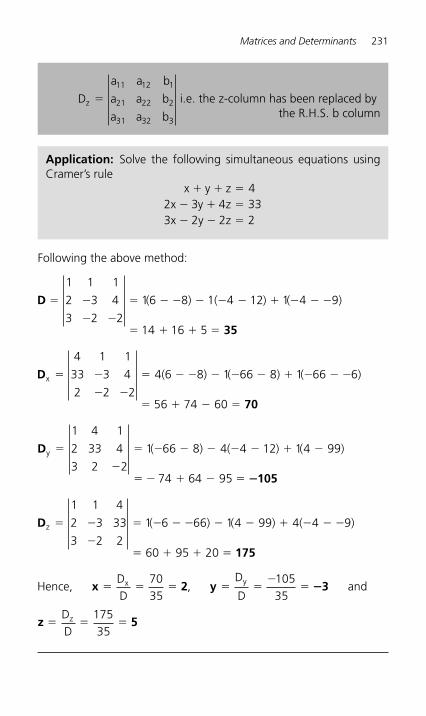
Matrices and Determinants 231
Following the above method:
D
35
� �
� �
� � � � � � � � � �
� � � �
1 1 1
2 3 4
3 2 2
16 8 4 12 1 4 9
14 16 5
( ) 1( ) ( )
D
70
x ( ) ( ) ( )� �
� �
� � � � � � � � � �
� � � �
4 1 1
33 3 4
2 2 2
4 6 8 1 66 8 1 66 6
56 74 60
D
105
y ( ) ( ) ( )�
�
� � � � � � � �
� � � � �
1 4 1
2 33 4
3 2 2
1 66 8 4 4 12 1 4 99
74 64 95 �
D
175
z ( ) ( ) ( 4 )� �
�
� � � � � � � � � �
� � � �
1 1 4
2 3 33
3 2 2
1 6 66 1 4 99 4 9
60 95 20
Hence, , andx 2 y 3� � � � �
��
DD
D
Dx y70
3510535
�
z 5� � �DD
z 17535
D
a a b
a a b
a a bz
11 12 1
21 22 2
31 32 3
� i.e. the z-column has been replaced bythe R.H.S. b column
Application: Solve the following simultaneous equations using Cramer’s rule
x y z2x y z3x 2y 2z
� � �
� � �
� � �
43 4 33
2
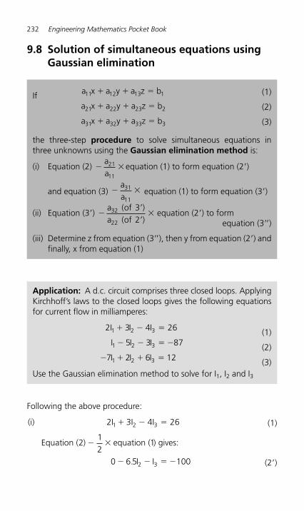
232 Engineering Mathematics Pocket Book
9.8 Solution of simultaneous equations using Gaussian elimination
If a x a y a z b11 12 13 1� � � (1)
a x a y a z b21 22 23 2� � � (2)
a x a y a z b31 32 33 3� � � (3)
the three-step procedure to solve simultaneous equations in three unknowns using the Gaussian elimination method is:
(i) Equation (2) � �aa
21
11
equation (1) to form equation (2 � )
and equation (3) � �aa
31
11 equation (1) to form equation (3 � )
(ii) Equation (3 � ) ��
��
a ofa of22
32 32
( )( )
equation (2 � ) to form equation (3� � )
(iii) Determine z from equation (3 � �), then y from equation (2 �) and finally, x from equation (1)
Application: A d.c. circuit comprises three closed loops. Applying Kirchhoff’s laws to the closed loops gives the following equations for current flow in milliamperes:
2I I I1 2 33 4 26� � � (1)
I I I1 2 35 3 87� � � � (2) � � � �7 2 6 121 2 3I I I (3)
Use the Gaussian elimination method to solve for I 1 , I 2 and I 3
Following the above procedure:
(i) 2I 3I 4I1 � � �2 3 26 (1)
Equation ( ) equation ( ) gives:
0 . I I
212
1
6 5 1002 3
� �
� � � � (2�)
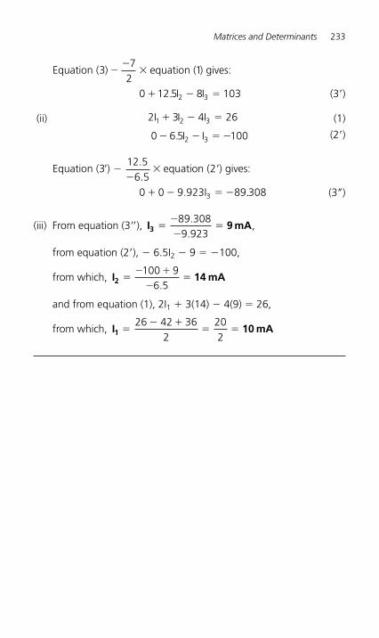
Matrices and Determinants 233
Equation ( ) equation ( ) gives:
0 .
37
21
12 5 8 1032 3
��
�
� � �I I (3� )
(ii) 2I I I1 2 33 4 26� � � (1)
0 .� � � �6 5 1002 3I I (2� )
Equation (3 ) equation ( ) gives:
0 0 9.923I
� ���
�
� � � �
12 56 5
2
893
..
..308 (3� � )
(iii) From equation (3 � � ), I 9 mA3 ��
��
89 3089 923
..
,
from equation (2 � ), � 6.5I 2 � 9 � � 100,
from which, I 14 mA2 �� �
��
100 96 5.
and from equation (1), 2I 1 � 3(14) � 4(9) � 26,
from which, I 10 mA1 �� �
� �26 42 36
2202
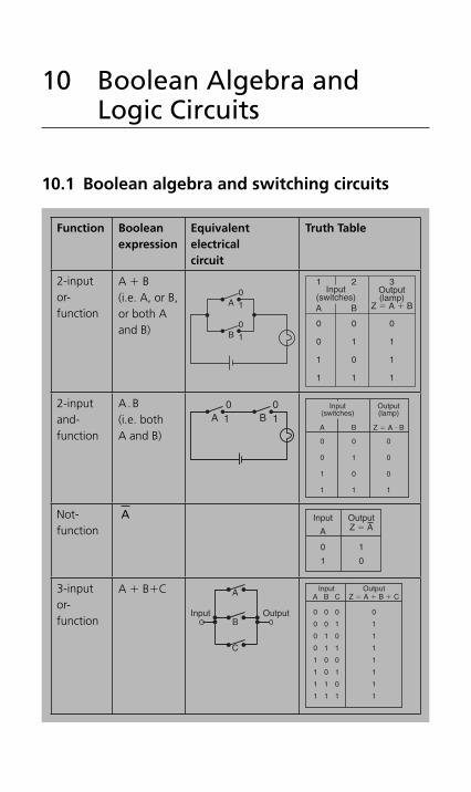
10 Boolean Algebra and Logic Circuits
10.1 Boolean algebra and switching circuits
Function Booleanexpression
Equivalent electricalcircuit
Truth Table
2-input or-function
A � B(i.e. A, or B, or both A and B)
01
01B
A
1
A B
2 3Output(lamp)
Z � A � B
0 0 0
0 1 1
1 0 1
1 1 1
Input(switches)
2-input and-function
A . B(i.e. both A and B)
0 011 BA
A B
Output(lamp)
Z � A � B
0 0 0
0 1 0
1 0 0
1 1 1
Input(switches)
Not-function
A A
0 1
1 0
Input OutputZ � A
3-input or-function
A � B � C
OutputInput
A
B
C
InputA B C
00 0 0
00 1 1
10 0 1
10 1 1
01 0 1
01 1 1
11 0 1
11 1 1
OutputZ � A � B � C
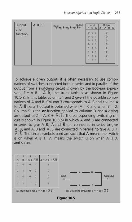
Boolean Algebra and Logic Circuits 235
3-input and-function
A . B . C OutputInputA B C
InputA B C
00 0 0
00 1 0
10 0 0
10 1 0
01 0 0
01 1 0
11 0 0
11 1 1
OutputZ � A � B � C
To achieve a given output, it is often necessary to use combi-nations of switches connected both in series and in parallel. If the output from a switching circuit is given by the Boolean expres-sion: Z � A . B � A . B , the truth table is as shown in Figure 10.5(a) . In this table, columns 1 and 2 give all the possible combi-nations of A and B. Column 3 corresponds to A . B and column 4 to A . B i.e. a 1 output is obtained when A � 0 and when B � 0. Column 5 is the or-function applied to columns 3 and 4 giving an output of Z � A . B � A . B . The corresponding switching cir-cuit is shown in Figure 10.5(b) in which A and B are connected in series to give A . B, A and B are connected in series to give A . B , and A . B and A . B are connected in parallel to give A . B � A . B . The circuit symbols used are such that A means the switch is on when A is 1, A means the switch is on when A is 0, and so on.
0 0
0 1
1 0
1 2A B
1 1
0 1
0 0
0 0
3 4A�B A�B
1 0
1
5
0
0
1
(a) Truth table for Z � A�B � A�B
Z � A�B � A�B
BA
BA
Input Output Z
(b) Switching circuit for Z � A�B � A�B
Figure 10.5
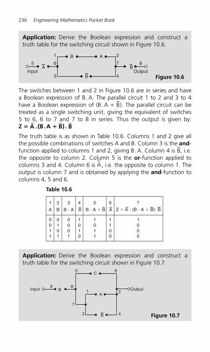
236 Engineering Mathematics Pocket Book
The switches between 1 and 2 in Figure 10.6 are in series and have a Boolean expression of B . A. The parallel circuit 1 to 2 and 3 to 4 have a Boolean expression of (B . A � B ). The parallel circuit can be treated as a single switching unit, giving the equivalent of switches 5 to 6, 6 to 7 and 7 to 8 in series. Thus the output is given by: Z � A . (B . A � B ) . B
The truth table is as shown in Table 10.6 . Columns 1 and 2 give all the possible combinations of switches A and B. Column 3 is the and -function applied to columns 1 and 2, giving B . A. Column 4 is B , i.e. the opposite to column 2. Column 5 is the or-function applied to columns 3 and 4. Column 6 is A , i.e. the opposite to column 1. The output is column 7 and is obtained by applying the and-function to columns 4, 5 and 6.
Application: Derive the Boolean expression and construct a truth table for the switching circuit shown in Figure 10.6 .
AB
B
A B
4
7 8
Output
5
Input
2
3
6
1
Figure 10.6
Table 10.6
1
0011
1010
1011
1100
1000
0101
0001
A B B � A
2 3 4 5 6 7
B AB � A � B Z � A � (B � A � B)� B
Application: Derive the Boolean expression and construct a truth table for the switching circuit shown in Figure 10.7 .
AB
C
B
OutputInput
7
3
6
21
4
5
89
Figure 10.7
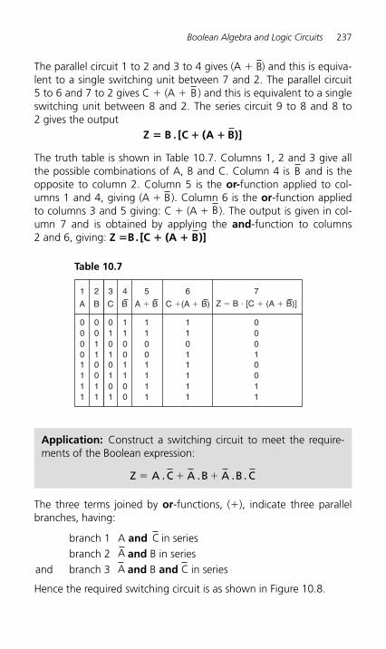
Boolean Algebra and Logic Circuits 237
The parallel circuit 1 to 2 and 3 to 4 gives (A � B ) and this is equiva-lent to a single switching unit between 7 and 2. The parallel circuit 5 to 6 and 7 to 2 gives C � (A � B ) and this is equivalent to a single switching unit between 8 and 2. The series circuit 9 to 8 and 8 to 2 gives the output
Z B . [C (A B)]� � �
The truth table is shown in Table 10.7 . Columns 1, 2 and 3 give all the possible combinations of A, B and C. Column 4 is B and is the opposite to column 2. Column 5 is the or-function applied to col-umns 1 and 4, giving (A � B ). Column 6 is the or-function applied to columns 3 and 5 giving: C � (A � B ). The output is given in col-umn 7 and is obtained by applying the and-function to columns 2 and 6, giving: Z � B . [C � (A � B )]
Table 10.7
1
0000
1100
1100
1101
0001
0011
0101
1111
1100
1111
1111
0011
0011
0101
A B C
2 43 5 6 7
B A � B Z � B � [C � (A � B)]C �(A � B)
Application: Construct a switching circuit to meet the require-ments of the Boolean expression:
Z A . C A .B A .B . C� � �
The three terms joined by or-functions, ( �), indicate three parallel branches, having:
branch 1 A and C in series branch 2 A and B in series and branch 3 A and B and C in series
Hence the required switching circuit is as shown in Figure 10.8 .
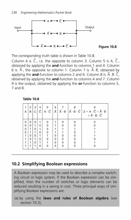
238 Engineering Mathematics Pocket Book
The corresponding truth table is shown in Table 10.8 . Column 4 is C , i.e. the opposite to column 3 . Column 5 is A . C , obtained by applying the and-function to columns 1 and 4 . Column 6 is A , the opposite to column 1 . Column 7 is A .B , obtained by applying the and-function to columns 2 and 6. Column 8 is A .B .C , obtained by applying the and-function to columns 4 and 7 . Column 9 is the output, obtained by applying the or-function to columns 5, 7 and 8 .
A
A
A C
B
B
C
OutputInput
Figure 10.8
10.2 Simplifying Boolean expressions
A Boolean expression may be used to describe a complex switch-ing circuit or logic system. If the Boolean expression can be sim-plified, then the number of switches or logic elements can be reduced resulting in a saving in cost. Three principal ways of sim-plifying Boolean expressions are:
(a) by using the laws and rules of Boolean algebra (see section 10.3),
Table 10.8
1
0000
1010
0000
0010
0011
0011
0101
1111
1010
1010
0000
1010
0011
0101
A B C
2 43 5 8 9
C
11110000
6
AA � C
00110000
7
A � B Z � A � C � A � B� A � B � C
A � B � C
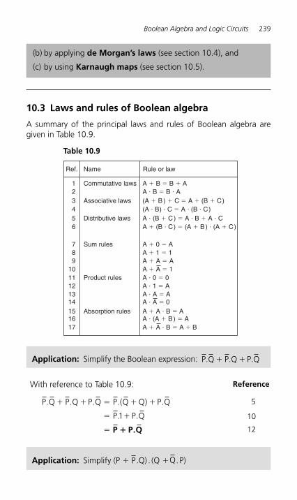
Boolean Algebra and Logic Circuits 239
10.3 Laws and rules of Boolean algebra
A summary of the principal laws and rules of Boolean algebra are given in Table 10.9 .
Application: Simplify the Boolean expression: P.Q P.Q P.Q� �
Table 10.9
Ref. Name
Commutative laws123456
A � B � B � AA � B � B � A(A � B ) � C � A � (B � C)(A � B) � C � A � (B � C)A � (B � C) � A � B � A � CA � (B � C) � (A � B ) � (A � C)
789
1011121314151617
Associative laws
Distributive laws
Sum rules
Product rules
Absorption rules
Rule or law
A � 0 � AA � 1 � 1A � A � AA � A � 1A � 0 � 0A � 1 � AA � A � AA � A � 0A � A � B � AA � (A � B) � AA � A � B � A � B
With reference to Table 10.9 : Reference
P.Q P.Q P.Q P.(Q Q) P.Q
P. P.Q
� � � � �
� �
�
1
P P.Q�
5
10
12
Application: Simplify (P � P .Q) . (Q � Q . P)
(b) by applying de Morgan’s laws (see section 10.4), and
(c) by using Karnaugh maps (see section 10.5).
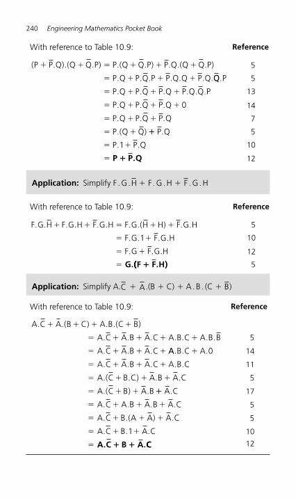
240 Engineering Mathematics Pocket Book
With reference to Table 10.9 : Reference
F.G.H F.G.H F.G.H F.G.(H H) F.G.H
F.G.1 F.G.H
F.G F.G.H
� � � � �
� �
� �
� G.((F F.H)�
5
10
12
5
With reference to Table 10.9 : Reference
(P P.Q).(Q Q.P) P.(Q Q.P) P.Q.(Q Q.P)
P.Q P.Q.P P.Q.Q P.Q.
� � � � � �
� � � � QQ.P
P.Q P.Q P.Q P.Q.Q.P
P.Q P.Q P.Q 0
P.Q P.Q P.Q
P.(Q Q)
� � � �
� � � �
� � �
� � ��
� �
�
P.Q
P.1 P.Q
P P.Q�
5
5
13
14
7
5
10
12
Application: Simplify F . G . H � F . G . H � F . G . H
Application: Simplify A. C � A .(B � C) � A . B . (C � B )
With reference to Table 10.9 : Reference
A.C A.(B C) A.B.(C B)
A.C A.B A.C A.B.C A.B.B
A.C A.B A.C
� � � �
� � � � �
� � � � AA.B.C A.0
A.C A.B A.C A.B.C
A.(C B.C) A.B A.C
A.(C B) A.B
�
� � � �
� � � �
� � � ��
� � � �
� � � �
� � �
�
A.C
A.C A.B A.B A.C
A.C B.(A A) A.C
A.C B.1 A.C
A.C B A.� � CC
5
14
11
5
17
5
5
10
12
Boolean Algebra and Logic Circuits 241
10.4 De Morgan’s laws
De Morgan’s laws state that:
A B . and A .B� � � �A B A B
Application: Simplify the Boolean expression A .B A B� � by using de Morgan’s laws and the rules of Boolean algebra
Applying de Morgan’s law to the first term gives:
A .B A B A B since A A� � � � � Applying de Morgan’s law to the second term gives:
A B A . B A . B� � �
Thus, A .B A B (A B) A . B� � � � �
Removing the bracket and reordering gives: A � A. B � B
But, by rule 15, Table 10.9 , A � A . B � A. It follows that:
A � A . B � A
Thus: A .B A B A B� � � �
Application: Simplify the Boolean expression ( )A.B C .(A B.C)� � by using de Morgan’s laws and the rules of Boolean algebra
Applying de Morgan’s laws to the first term gives:
( )A . B C A . B .C (A B) .C (A B) .C A .C B.C� � � � � � � � Applying de Morgan’s law to the second term gives:
( ) ( )A B .C A B C A (B C)� � � � � � �
Thus ( )A . B C (A B .C) (A .C B.C) . (A B C)
A . A .C A . B .C A .C.C
A .B .C
� � � � � �
� � �
� � BB. B .C B .C.C�
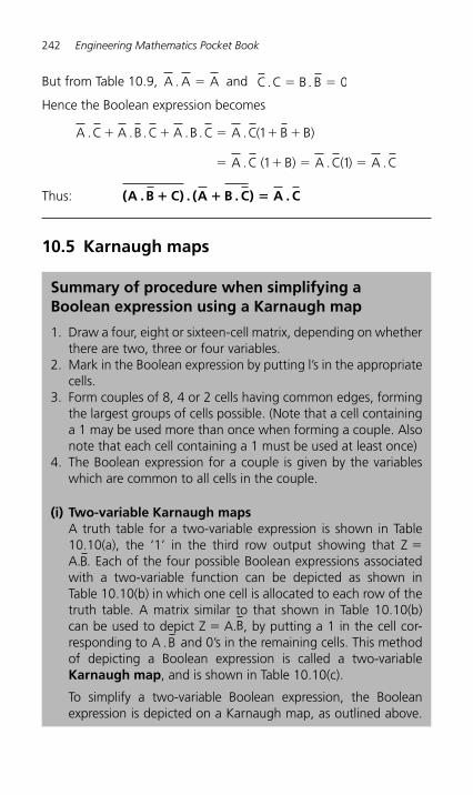
242 Engineering Mathematics Pocket Book
But from Table 10.9 , A . A A� and C.C B . B� � 0
Hence the Boolean expression becomes
A C A B C A C A C B
A C A C A C
. . . .B . . ( B)
. ( B) . ( ) .
� � � � �
� � � �
1
1 1
Thus: ( B ) ( C) A CA . C . A B . .� � �
10.5 Karnaugh maps
Summary of procedure when simplifying a Boolean expression using a Karnaugh map
1. Draw a four, eight or sixteen-cell matrix, depending on whether there are two, three or four variables.
2. Mark in the Boolean expression by putting l’s in the appropriate cells.
3. Form couples of 8, 4 or 2 cells having common edges, forming the largest groups of cells possible. (Note that a cell containing a 1 may be used more than once when forming a couple. Also note that each cell containing a 1 must be used at least once)
4. The Boolean expression for a couple is given by the variables which are common to all cells in the couple.
(i) Two-variable Karnaugh maps A truth table for a two-variable expression is shown in Table 10.10(a) , the ‘ 1 ’ in the third row output showing that Z � A.B . Each of the four possible Boolean expressions associated with a two-variable function can be depicted as shown in Table 10.10(b) in which one cell is allocated to each row of the truth table. A matrix similar to that shown in Table 10.10(b) can be used to depict Z � A. B , by putting a 1 in the cell cor-responding to A .B and 0’s in the remaining cells. This method of depicting a Boolean expression is called a two- variableKarnaugh map , and is shown in Table 10.10(c) .
To simplify a two-variable Boolean expression, the Boolean expression is depicted on a Karnaugh map, as outlined above.
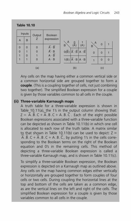
Boolean Algebra and Logic Circuits 243
Any cells on the map having either a common vertical side or a common horizontal side are grouped together to form a c ouple. (This is a coupling together of cells, not just combining two together). The simplified Boolean expression for a couple is given by those variables common to all cells in the couple.
(ii) Three-variable Karnaugh maps A truth table for a three-variable expression is shown in Table 10.11(a) , the 1’s in the output column showing that: Z � A .B .C A .B .C A .B .C� � . Each of the eight possible Boolean expressions associated with a three-variable function can be depicted as shown in Table 10.11(b) in which one cell is allocated to each row of the truth table. A matrix similar to that shown in Table 10.11(b) can be used to depict: Z � A .B .C A .B .C A .B .C� � , by putting 1’s in the cells corre-sponding to the Boolean terms on the right of the Boolean equation and 0’s in the remaining cells. This method of depicting a three-variable Boolean expression is called a three-variable Karnaugh map, and is shown in Table 10.11(c) .
To simplify a three-variable Boolean expression, the Boolean expression is depicted on a Karnaugh map as outlined above. Any cells on the map having common edges either vertically or horizontally are grouped together to form couples of four cells or two cells. During coupling the horizontal lines at the top and bottom of the cells are taken as a common edge, as are the vertical lines on the left and right of the cells. The simplified Boolean expression for a couple is given by those variables common to all cells in the couple.
Table 10.10
Inputs
A B
0 0 0
Booleanexpression
OutputZ
A � B
(a)
A � B0 1 0 A � B1 0 1
A � B1 1 0
AB
0(B)
0(A)
(b)
1(A)
1(B)
A � B
A � B
A � B
A � B
(c)
AB
0
0 1
0 1
0 01
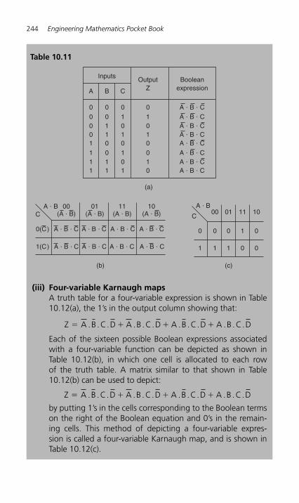
244 Engineering Mathematics Pocket Book
(iii) Four-variable Karnaugh maps A truth table for a four-variable expression is shown in Table 10.12(a) , the 1’s in the output column showing that:
Z � � � �A .B .C.D A .B .C.D A .B .C.D A .B .C.D Each of the sixteen possible Boolean expressions associated with a four-variable function can be depicted as shown in Table 10.12(b) , in which one cell is allocated to each row of the truth table. A matrix similar to that shown in Table 10.12(b) can be used to depict:
Z A .B .C.D A .B .C.D A .B .C.D A .B .C.D� � � � by putting 1’s in the cells corresponding to the Boolean terms on the right of the Boolean equation and 0’s in the remain-ing cells. This method of depicting a four-variable expres-sion is called a four-variable Karnaugh map, and is shown in Table 10.12(c) .
Table 10.11
Inputs
0
Booleanexpression
OutputZ
A � B � C
A � B � CA � B � CA � B � C
(a)
10
A
0
000
B
0
011
C
0
101 1
0 A � B � C
A � B � CA � B � CA � B � C
01
1
111
0
011
0
101 0
A � BC
0(C)
00(A � B)
(b)
1(C)
A � B � C
A � B � C
01(A � B)
A � B � C
A � B � C
11(A � B)
A � B � C
A � B � C
10(A � B)
A � B � C
A � B � C
(c)
A � B
C
0
00
0
1
01
0
1
11
1
0
10
0
01
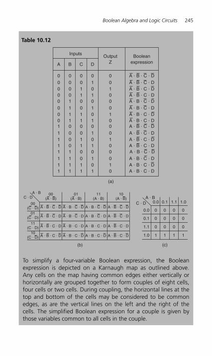
Boolean Algebra and Logic Circuits 245
To simplify a four-variable Boolean expression, the Boolean expression is depicted on a Karnaugh map as outlined above. Any cells on the map having common edges either vertically or horizontally are grouped together to form couples of eight cells, four cells or two cells. During coupling, the horizontal lines at the top and bottom of the cells may be considered to be common edges, as are the vertical lines on the left and the right of the cells. The simplified Boolean expression for a couple is given by those variables common to all cells in the couple.
Table 10.12
Inputs
0
Booleanexpression
OutputZ
A � B � C � D
A � B � C � DA � B � C � DA � B � C � DA � B � C � D
A � B � C � DA � B � C � DA � B � C � D
(a)
01
B
0
000
C
0
011
D
0
101 0
0
01
1
111
0
011
A
0
0000
000
0
101 0
0 A � B � C � D
A � B � C � DA � B � C � DA � B � C � DA � B � C � D
A � B � C � DA � B � C � DA � B � C � D
01
0
000
0
011
0
101 0
0
01
1
111
0
011
1
1111
111
0
101 0
A � B 00(A � B)
00(C � D)
10(C � D)
01(C � D)
11(C � D)
(b)
A � B � C � D
A � B � C � D
A � B � C � D
A � B � C � D
A � B � C � D
A � B � C � D
A � B � C � D
A � B � C � D
A � B � C � D
A � B � C � D
A � B � C � D
A � B � C � D
A � B � C � D
A � B � C � D
A � B � C � D
A � B � C � D
01(A � B)
11(A � B)
10(A � B)C � D
(c)
A � B
0.0
0.0
0
0
0.1
0
0
1.1
0
0
1.0
0
00.1
0 0 0 01.1
1 1 1 11.0
C � D
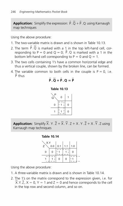
246 Engineering Mathematics Pocket Book
Using the above procedure:
1. The two-variable matrix is drawn and is shown in Table 10.13 .
2. The term P .Q is marked with a 1 in the top left-hand cell, cor-responding to P � 0 and Q � 0; P .Q is marked with a 1 in the bottom left-hand cell corresponding to P � 0 and Q � 1.
3. The two cells containing 1’s have a common horizontal edge and thus a vertical couple, shown by the broken line, can be formed.
4. The variable common to both cells in the couple is P � 0, i.e. P thus
P . Q P . Q P� �
Table 10.13
0 1
0
1
0
0
1
1
PQ
Application: Simplify the expression: P .Q P .Q� using Karnaugh map techniques
Using the above procedure:
1. A three-variable matrix is drawn and is shown in Table 10.14 .
2. The 1’s on the matrix correspond to the expression given, i.e. for X .Y. Z , X � 0, Y � 1 and Z � 0 and hence corresponds to the cell in the top row and second column, and so on.
Application: Simplify X . Y . Z X . Y . Z X . Y . Z X . Y . Z� � � using Karnaugh map techniques
Table 10.14
0.0 0.1
0
1
1
0
1.1
1
0
1.0
0
1
0
1
X.YZ
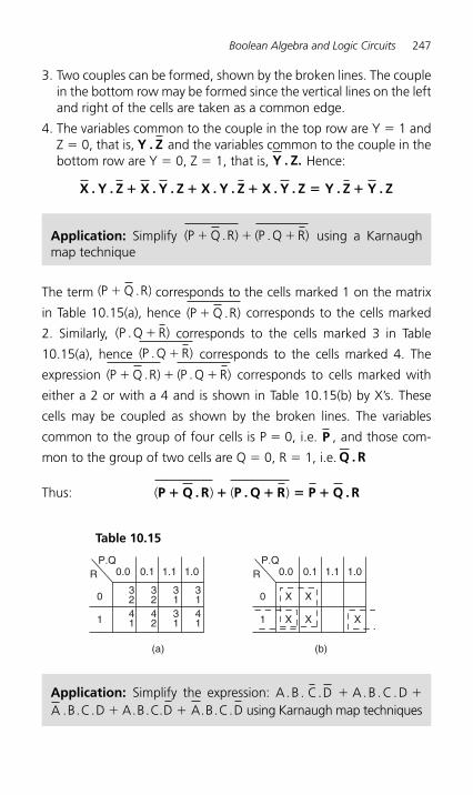
Boolean Algebra and Logic Circuits 247
3. Two couples can be formed, shown by the broken lines. The couple in the bottom row may be formed since the vertical lines on the left and right of the cells are taken as a common edge.
4. The variables common to the couple in the top row are Y � 1 and Z � 0, that is, Y . Z and the variables common to the couple in the bottom row are Y � 0, Z � 1, that is, Y . Z. Hence:
X Z X Y Z Y Z Y. Y . . . Z X . Y . X . . Z Y . . Z� � � � �
Application: Simplify ( ) ( )P Q .R P .Q R� � � using a Karnaugh map technique
The term ( . )P R� Q corresponds to the cells marked 1 on the matrix
in Table 10.15(a) , hence ( )P Q .R� corresponds to the cells marked
2. Similarly, (P .Q R)� corresponds to the cells marked 3 in Table
10.15(a), hence ( )P .Q R� corresponds to the cells marked 4. The
expression ( ) ( )P Q .R P .Q R� � � corresponds to cells marked with
either a 2 or with a 4 and is shown in Table 10.15(b) by X’s. These
cells may be coupled as shown by the broken lines. The variables
common to the group of four cells is P � 0, i.e. P , and those com-
mon to the group of two cells are Q � 0, R � 1, i.e. Q . R
Thus: ( ) ( )P Q . R P . Q R P Q . R� � � � �
Table 10.15
0.0
(a)
0.1
0
1
1.1 1.0
3241
3242
3131
3141
P.QR 0.0
(b)
0.1
0 X X
X X X1
1.1 1.0P.Q
R
Application: Simplify the expression: A . B . C.D � A . B . C . D � A . B . C . D � A . B . C.D � A . B . C .D using Karnaugh map techniques
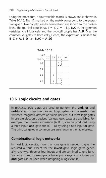
248 Engineering Mathematics Pocket Book
Using the procedure, a four-variable matrix is drawn and is shown in Table 10.16 . The 1’s marked on the matrix correspond to the expres-sion given. Two couples can be formed and are shown by the broken lines. The four-cell couple has B � 1, C � 1, i.e. B . C as the common variables to all four cells and the two-cell couple has A . B . D as the common variables to both cells. Hence, the expression simplifies to: B . C � A . B . D i.e. B . (C � A . D )
Table 10.16
0.0 0.1
0.0
0.1
1.1 1 1
1
1 11.0
1.1 1.0A.B
C.D
10.6 Logic circuits and gates
In practice, logic gates are used to perform the and, or and not-functions introduced earlier. Logic gates can be made from switches, magnetic devices or fluidic devices, but most logic gates in use are electronic devices. Various logic gates are available. For example, the Boolean expression (A . B . C) can be produced using a three-input, and-gate and (C � D) by using a two-input or-gate. The principal gates in common use are shown in the table below.
Combinational logic networks
In most logic circuits, more than one gate is needed to give the required output. Except for the invert-gate, logic gates gener-ally have two, three or four inputs and are confined to one func-tion only. Thus, for example, a two-input, or-gate or a four-input and -gate can be used when designing a logic circuit.
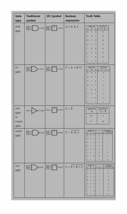
Gate
type
Traditional
symbol
IEC Symbol Boolean
expression
Truth Table
and-
gate
AB ZC
AB Z
&
C
Z � A . B . C INPUTSB
OUTPUTZ � A � B � CA C
00 0
00 1
10 0
10 1
01 0
01 1
11 0
11 1
0
0
0
0
0
0
0
1
or-
gate
AB ZC
AB Z
�1
C
Z � A � B � C INPUTSB
OUTPUTZ � A � B � CA C
00 0
00 1
10 0
10 1
01 0
01 1
11 0
11 1
0
1
1
1
1
1
1
1
not-
gate
or
invert-
gate
A Z A Z�1 Z � A INPUTS OUTPUT
Z � AA
0
1
1
0
nand-
gate
AB ZC
AB Z
&
C Z � A .B . C
INPUTSB
OUTPUTZ � A � B � CA � B � CA C
00 0
00 1
10 0
10 1
01 0
01 1
11 0
11
0
0
0
0
0
0
0
11
1
1
1
1
1
1
1
0
nor-
gate
AB ZC
AB Z
�1
CZ � A B C� �
INPUTSB
OUTPUTZ�A�B�CA�B�CA C
00 0
00 1
10 0
10 1
01 0
01 1
11 0
11
0
1
1
1
1
1
1
11
1
0
0
0
0
0
0
0
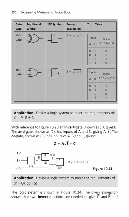
250 Engineering Mathematics Pocket Book
Gate
type
Traditional
symbol
IEC Symbol Boolean
expression
Truth Table
xor-gate
�1 Z � A B⊕ Inputs
0
Output
Z �A XOR B
11
A
0
011
B
0
101 0
xnor-gate
�1 Z � A B⊕ Inputs
1
Output
Z �A XNOR B
00
A
0
011
B
0
101 1
With reference to Figure 10.23 an invert-gate, shown as (1), gives B .The and-gate, shown as (2), has inputs of A and B , giving A . B . The or- gate, shown as (3), has inputs of A . B and C, giving:
Z A .B C� �
Application: Devise a logic system to meet the requirements of: Z � A .B � C
Application: Devise a logic system to meet the requirements of
(P Q) . (R S)� �
1
A
B
C(1) (3)
(2)
&B
A�B
Z � A�B � C
Figure 10.23
The logic system is shown in Figure 10.24 . The given expression shows that two invert-functions are needed to give Q and R and
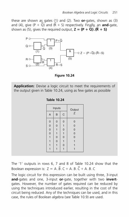
Boolean Algebra and Logic Circuits 251
these are shown as gates (1) and (2). Two or-gates, shown as (3) and (4), give (P � Q ) and ( R � S) respectively. Finally, an and -gate, shown as (5), gives the required output, Z � (P � Q ) . ( R � S)
&
P
Q
R
S
(1)
(2)
(3)
(5)
1
(4)
1
Q
R
P�Q
R�S
Z � (P�Q)�(R�S)
Figure 10.24
Application: Devise a logic circuit to meet the requirements of the output given in Table 10.24 , using as few gates as possible
Table 10.24
Inputs
0
OutputZ
00
A
0
000
B
0
011
C
0
101 0
0
11
1
111
0
011
0
101 1
The ‘ 1 ’ outputs in rows 6, 7 and 8 of Table 10.24 show that the Boolean expression is: Z A .B .C A .B .C A .B .C� � �
The logic circuit for this expression can be built using three, 3-input and-gates and one, 3-input or-gate, together with two invert -gates. However, the number of gates required can be reduced by using the techniques introduced earlier, resulting in the cost of the circuit being reduced. Any of the techniques can be used, and in this case, the rules of Boolean algebra (see Table 10.9 ) are used.
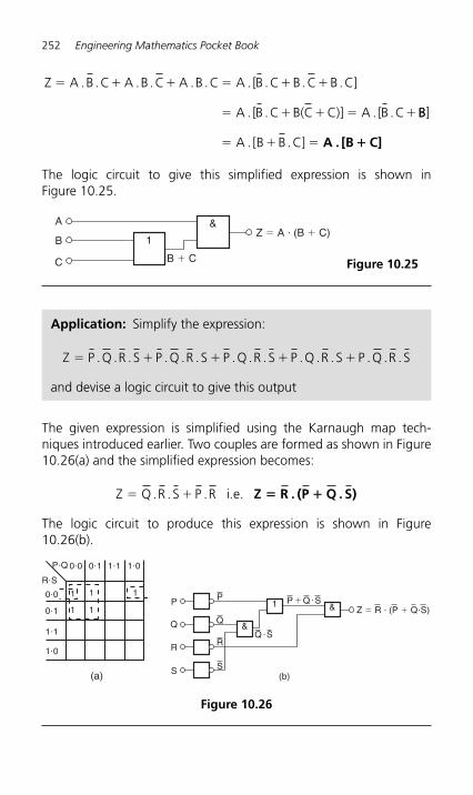
252 Engineering Mathematics Pocket Book
Z A .B .C A .B .C A .B .C A . [B .C B .C B.C]
A . [B .C B(C C)] A . [B .C
� � � � � �
� � � � �BB]
A . [B B .C]� � � A [B C]. �
The logic circuit to give this simplified expression is shown in Figure 10.25 .
&A
B
C
1Z � A � (B � C)
B � C Figure 10.25
Application: Simplify the expression:
Z P .Q .R .S P .Q .R .S P .Q .R .S P .Q .R .S P .Q .R .S� � � � �
and devise a logic circuit to give this output
The given expression is simplified using the Karnaugh map tech-niques introduced earlier. Two couples are formed as shown in Figure 10.26(a) and the simplified expression becomes:
Z Q .R .S P .R i.e.� � Z . (P Q . S)� �R
The logic circuit to produce this expression is shown in Figure 10.26(b) .
(a)
R�S
P�Q
0�0
0�0 0�1 1�1 1�0
11
11
1
0�1
1�1
1�0
Figure 10.26
P
Q
R
S
P
Q
Q SR
S
1
(b)
&
&
�
Q S�P �Z � R � (P � Q�S)
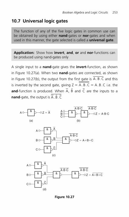
Boolean Algebra and Logic Circuits 253
10.7 Universal logic gates
Figure 10.27
&A
(a)
Z � A &&ABC
(b)
Z � A�B�C
A�B�C A�B�C
A
B
C
&A
& &B
&C
(c)
Z � A�B�C
A�B�C
(d)
A
B
C
&A
& & &B
&C
Z � A�B�C
A�B�C A�B�C
The function of any of the five logic gates in common use can be obtained by using either nand-gates or nor-gates and when used in this manner, the gate selected is called a universal gate .
Application: Show how invert, and, or and nor-functions can be produced using nand-gates only
A single input to a nand-gate gives the invert-function, as shown
in Figure 10.27(a) . When two nand-gates are connected, as shown
in Figure 10.27(b) , the output from the first gate is A .B .C and this
is inverted by the second gate, giving Z � A .B .C � A . B . C i.e. the
and-function is produced. When A , B and C are the inputs to a
nand -gate, the output is A .B .C
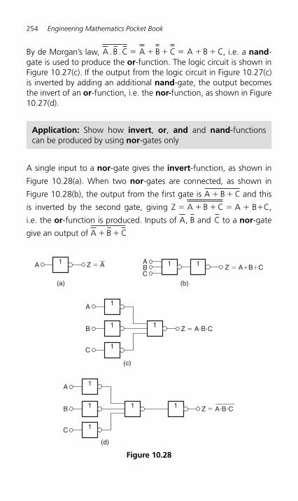
254 Engineering Mathematics Pocket Book
By de Morgan’s law, A .B .C A B C A B C� � � � � � , i.e. a nand -gate is used to produce the or-function. The logic circuit is shown in Figure 10.27(c) . If the output from the logic circuit in Figure 10.27(c) is inverted by adding an additional nand-gate, the output becomes the invert of an or-function, i.e. the nor-function, as shown in Figure 10.27(d) .
Application: Show how invert, or, and and nand -functions can be produced by using nor -gates only
A single input to a nor-gate gives the invert-function, as shown in
Figure 10.28(a) . When two nor-gates are connected, as shown in
Figure 10.28(b) , the output from the first gate is A B C� � and this
is inverted by the second gate, giving Z � A B C� � � A � B �C,
i.e. the or-function is produced. Inputs of A , B and C to a nor -gate
give an output of A B C� �
Figure 10.28
1A
(a)
Z � A 11ABC
(b)
Z � A�B�C
1A
1 1B
1C
(c)
Z � A�B�C
(d)
1A
1 1 1B
1C
Z � A�B�C
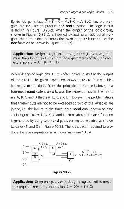
Boolean Algebra and Logic Circuits 255
By de Morgan’s law, A B C A .B .C A .B .C� � � � , i.e. the nor -gate can be used to produce the and-function. The logic circuit is shown in Figure 10.28(c) . When the output of the logic circuit, shown in Figure 10.28(c) , is inverted by adding an additional nor -gate, the output then becomes the invert of an or-function, i.e. the nor -function as shown in Figure 10.28(d) .
(2)
(1)
A &
(3)C
&
&&B
D
C
A�B,i.e.
A�B�C�D,i.e.Z�(A�B�C�D)
(A�B)A�B,i.e.
(A�B)
Figure 10.29
Application: Design a logic circuit, using nand-gates having not more than three inputs, to meet the requirements of the Boolean expression: Z � A B C D� � �
When designing logic circuits, it is often easier to start at the output
of the circuit. The given expression shows there are four variables
joined by or-functions. From the principles introduced above, if a
four-input nand-gate is used to give the expression given, the inputs
are A, B, C and D that is A, B, C and D. However, the problem states
that three-inputs are not to be exceeded so two of the variables are
joined, i.e. the inputs to the three-input nand-gate, shown as gate
(1) in Figure 10.29 , is A . B, C and D. From above, the and -function
is generated by using two nand-gates connected in series, as shown
by gates (2) and (3) in Figure 10.29 . The logic circuit required to pro-
duce the given expression is as shown in Figure 10.29 .
Application: Using nor-gates only, design a logic circuit to meet the requirements of the expression: Z D(A B C)� � �
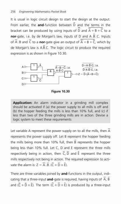
256 Engineering Mathematics Pocket Book
It is usual in logic circuit design to start the design at the output.
From earlier, the and-function between D and the terms in the
bracket can be produced by using inputs of D and A B C� � to a
nor-gate, i.e. by de Morgan’s law, inputs of D and A . B . C. Inputs
of A . B and C to a nor-gate give an output of A B C� � , which by
de Morgan’s law is A. B .C. The logic circuit to produce the required
expression is as shown in Figure 10.30 .
1
&
C
1A
B 1
DC
AA�B�C, i.e.A�B�C
D�A�B�C, i.e.
D�A�B�C, i.e.
Z � D�(A�B�C)
Figure 10.30
Application: An alarm indicator in a grinding mill complex should be activated if (a) the power supply to all mills is off and (b) the hopper feeding the mills is less than 10% full, and (c) if less than two of the three grinding mills are in action. Devise a logic system to meet these requirements
Let variable A represent the power supply on to all the mills, then A
represents the power supply off. Let B represent the hopper feeding
the mills being more than 10% full, then B represents the hopper
being less than 10% full. Let C, D and E represent the three mills
respectively being in action, then C, D and E represent the three
mills respectively not being in action. The required expression to acti-
vate the alarm is: Z � A .B . C D E( )� � .
There are three variables joined by and-functions in the output, indi-
cating that a three-input and-gate is required, having inputs of A, B
and ( )C D E� � . The term ( )C E� �D is produced by a three-input

Boolean Algebra and Logic Circuits 257
nand-gate. When variables C, D and E are the inputs to a nand -
gate, the output is C . D . E, which, by De Morgan’s law is ( )C D E� � .
Hence the required logic circuit is as shown in Figure 10.31 .
C
&
�1
�1
&
E
D
B
A
Z � A�B�(C�D�E)
i.e. (C � D � E)C � D � E
A
B
Figure 10.31
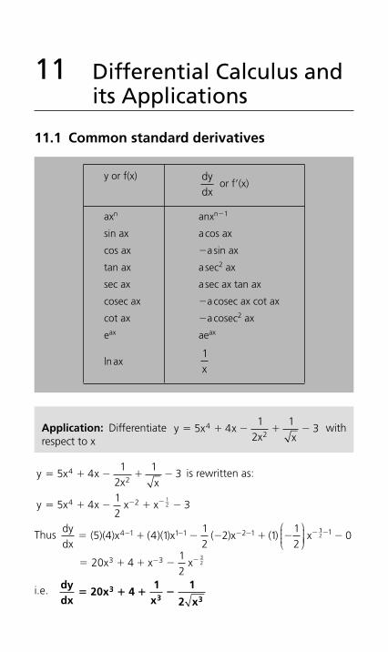
11 Differential Calculus and its Applications
11.1 Common standard derivatives
y x xx x
� � � � �5 41
21
342
is rewritten as:
y x� � � � �� �5 412
34 2 12x x x
Thus dydx
( )(4)x ( )( )x ( )x ( ) x� � � � � �� � � � �5 4 112
2 112
4 1 1 1 2 1⎛⎝⎜⎜⎜
⎞⎠⎟⎟⎟⎟
112 1 0� �
� � � �� �20 412
3 3 32x x x
i.e. dy
dx20x 4
x 2 x3
3� � � �
1 13
y or f(x)
dydx
or f � (x)
ax n anxn � 1
sin ax a cos ax
cos ax �a sin ax
tan ax a sec 2 ax
sec ax a sec ax tan ax
cosec ax � a cosec ax cot ax
cot ax �a cosec 2 ax
e ax aeax
ln ax
1x
Application: Differentiate y x xx x
� � � � �5 41
21
342
with respect to x
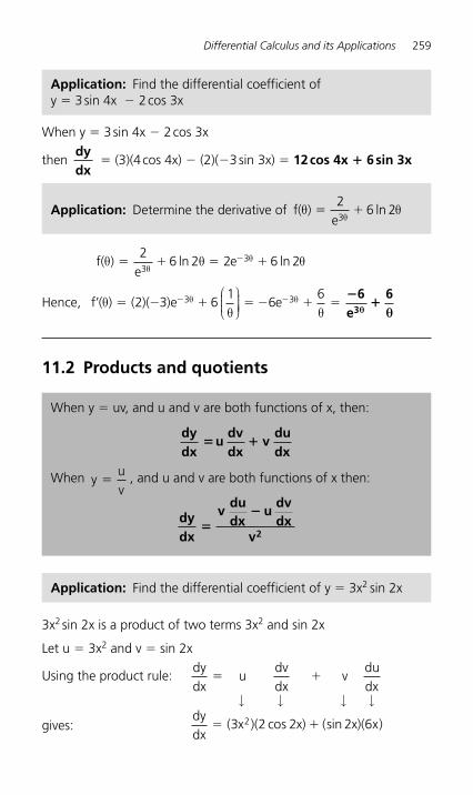
Differential Calculus and its Applications 259
When y � 3 sin 4x � 2 cos 3x
thendydx
� (3)(4 cos 4x) � (2)( �3 sin 3x) � 12 cos 4x � 6 sin 3x
Application: Find the differential coefficient of y � 3 sin 4x � 2 cos 3x
Application: Determine the derivative of f( )e
θ θθ
� �2
6 23
ln
f( )
e2 eθ θ θ
θθ� � � ��2
6 2 6 23
3ln ln
Hence, f ( ) ( )( )e e� � � � � � � �� �θθ θ
θ θ2 3 61
663 3
⎛⎝⎜⎜⎜
⎞⎠⎟⎟⎟⎟
��
6 6e3θ θ
11.2 Products and quotients
When y � uv, and u and v are both functions of x, then:
dydx
udvdx
vdudx
� �
When yuv
� , and u and v are both functions of x then:
dydx
vdudx
udvdx
v2�
�
Application: Find the differential coefficient of y � 3x 2 sin 2x
3x 2 sin 2x is a product of two terms 3x 2 and sin 2x
Let u � 3x 2 and v � sin 2x
Using the product rule: dydx
udvdx
vdudx
� �
↓ ↓ ↓ ↓
gives: dydx
( x )( x) ( x)( )� �3 2 2 2 62 cos sin x
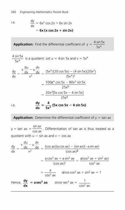
260 Engineering Mathematics Pocket Book
i.e. dydx
x x� �6 6 22 cos sin2x x
� 6x x 2x sin 2x( cos )�
Application: Find the differential coefficient of yx
x�
4 55 4
sin
4 55 4
sin xx
is a quotient. Let u � 4 sin 5x and v � 5x 4
dydx
vdudx
udvdx
vx x x x
x�
��
�
�
2
4 3
4 2
5 20 5 4 5 205
100
( )( cos ) ( sin )( )( )
xx x x xx
x x x xx
4 3
8
3
8
5 80 525
20 5 5 4 525
cos sin
[ cos sin ]
�
��
i.e. dydx
45x
(5x cos 5x 4 sin 5x)5
� �
Application: Determine the differential coefficient of y � tan ax
y � tan ax � sincos
axax
. Differentiation of tan ax is thus treated as a
quotient with u � sin ax and v � cos ax
dydx
vdudx
udvdx
vax a ax ax a ax
ax�
��
� �2
(cos )( cos ) (sin )( sin )(cos )22
2 2
2
2 2
2
2
��
��
�
a ax a axax
a ax axax
aax
cos sin(cos )
(cos sin )cos
cossiince cos sin2 2 1ax ax� �
Hence, dydx
� a sec 2 ax since sec 2 ax � 12cos ax
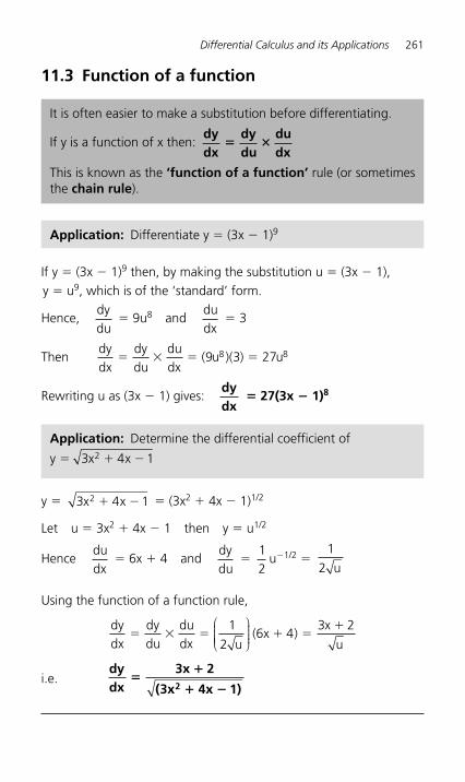
Differential Calculus and its Applications 261
11.3 Function of a function
It is often easier to make a substitution before differentiating.
If y is a function of x then: dydx
dydu
dudx
� �
This is known as the ‘ function of a function ’ rule (or sometimes the chain rule ).
Application: Differentiate y � (3x � 1) 9
If y � (3x � 1) 9 then, by making the substitution u � (3x � 1), y � u 9 , which is of the ‘ standard ’ form.
Hence,dydu
� 9u 8 anddudx
� 3
Thendydx
dudx
� � � �dydu
( u )( ) u9 3 278 8
Rewriting u as (3x � 1) gives: dydx
� 27(3x � 1) 8
Application: Determine the differential coefficient of
y � 3 4 12x x� �
y � 3 4 12x x� � � (3x 2 � 4x � 1) 1/2
Let u � 3x2 � 4x � 1 then y � u 1/2
Hence dudx
� 6x � 4 anddydu
�
12
u � 1/2 �
1
2 u
Using the function of a function rule,
dydx
dydu
dudx u
( x )x
u� � � � �
�1
26 4
3 2⎛
⎝⎜⎜⎜⎜
⎞
⎠⎟⎟⎟⎟
i.e. dydx
3x 2
3x 4x2�
�
� �( 1)
262 Engineering Mathematics Pocket Book
11.4 Successive differentiation
When a function y � f(x) is differentiated with respect to x the
differential coefficient is written as dydx
or f �(x). If the expression is
differentiated again, the second differential coefficient is obtained
and is written asd ydx
2
2 or f �(x). By successive differentiation further
higher derivatives such asd ydx
3
3 and
d ydx
4
4 may be obtained.
Thus, if y � 3x 4 , dydx
� 12x 3 , d ydx
2
2 � 36x 2 ,
d ydx
3
3 � 72x,
d ydx
4
4 � 72 andd ydx
5
5 � 0
Application: If f(x) � 2x 5 � 4x 3 � 3x � 5 determine f � (x)
If f(x) � 2x 5 � 4x 3 � 3x � 5
then f � (x) � 10x 4 � 12x 2 � 3
and f (x) � 40x 3 � 24x � 4x(10x2 � 6)
Application: Evaluate d yd
2
2θ when θ � 0 given y � 4 sec 2 θ
Since y � 4 sec 2 θ , then dydθ
� (4)(2)sec 2 θ tan 2 θ
� 8 sec 2 θ tan 2 θ (i.e. a product)
d yd
2
2θ � (8 sec 2 θ)(2 sec 2 2 θ ) � (tan 2 θ )[(8)(2)sec 2 θ tan 2 θ ]
� 16 sec 3 2 θ � 16 sec 2 θ tan 2 2 θ
When θ � 0,d y2
2dθ � 16 sec 3 0 � 16 sec 0 tan 2 0
� 16(1) � 16(1)(0) � 16
Differential Calculus and its Applications 263
11.5 Differentiation of hyperbolic functions
y or f(x)
dydx
or f� (x)
sinh ax a cosh ax
cosh ax a sinh ax
tanh ax a sech 2 ax
sech ax � a sech ax tanh ax
cosech ax � a cosech ax coth ax
coth ax �a cosech 2 ax
Application: Differentiate the following with respect to x:
(a) y � 4 sh 2x � 37
ch 3x (b) y � 5 th x2
� 2 coth 4x
(a)
dydx
� 4(2 cosh 2x) �
37
(3 sinh 3x) � 8 cosh 2x �
97
sinh 3x
(b) dydx
� 512 2
2sec hx⎛
⎝⎜⎜⎜
⎞⎠⎟⎟⎟⎟ � 2( �4 cosech 2 4x)
�
52
sec hx2
8 ech 4x2 2� cos
Application: Differentiate the following with respect to the variable:
(a) y � 4 sin 3t ch 4t (b) y � ln(sh 3 θ ) � 4 ch 2 3 θ
(a) y � 4 sin 3t ch 4t (i.e. a product)
dydx
t sh t ch t t
t sh t ch t
� �
� �
( sin )( ) ( )( )( cos )
sin c
4 3 4 4 4 4 3 3
16 3 4 12 4 oos 3t
� 4(4 sin 3t sh 4t 3cos 3t ch 4t)�
264 Engineering Mathematics Pocket Book
(b) y � ln(sh 3 θ ) � 4 ch 2 3 θ (i.e. a function of a function)
dyd sh
( ) ( )( ch )( sh )θ θ
θ θ θ
θ
� �
� �
13
3 3 4 2 3 3 3
3 3 2
⎛
⎝⎜⎜⎜⎜
⎞
⎠⎟⎟⎟⎟⎟
ch
coth 44 3 3ch θ θsh � 3( 3 8 ch 3 sh 3coth )θ θ θ�
11.6 Rates of change using differentiation
If a quantity y depends on and varies with a quantity x then the
rate of change of y with respect to x is dydx
. Thus, for example,
the rate of change of pressure p with height h is dpdh
.
A rate of change with respect to time is usually just called ‘ the
rate of change ’, the ‘with respect to time ’ being assumed. Thus,
for example, a rate of change of current, i, is didt
and a rate of
change of temperature, θ , is ddt
θ , and so on.
Application: Newtons law of cooling is given by θ � θ 0 e � kt , where the excess of temperature at zero time is θ 0°C and at time t seconds is θ°C. Determine the rate of change of temperature after 40 s, given that θ 0 � 16°C and k � � 0.03
The rate of change of temperature is ddt
θ
Since θ � θ 0 e � kt then ddt
θ � ( θ 0 )( � k)e � kt � � k θ 0 e � kt
When θ 0 � 16, k � � 0.03 and t � 40
thenddt
θ � � ( � 0.03)(16)e � ( � 0.03)(40)
� 0.48 e 1.2 � 1.594°C/s
Application: The luminous intensity I candelas of a lamp at vary-ing voltage V is given by: I � 4 � 10 � 4 V 2. Determine the voltage at which the light is increasing at a rate of 0.6 candelas per volt
Differential Calculus and its Applications 265
The rate of change of light with respect to voltage is given by dIdV
Since I � 4 � 10 � 4 V 2 , dIdV
� (4 � 10�4)(2) V � 8 � 10 � 4 V
When the light is increasing at 0.6 candelas per volt then
� 0.6 � 8 � 10 � 4 V, from which,
voltage V ��
� � ��
�0 68 10
0 075 104
4.. 750 volts
11.7 Velocity and acceleration
If a body moves a distance x metres in a time t seconds then:
(i) distance, x � f(t)
(ii) velocity, v � f �(t) or dxdt
, which is the gradient of the distance/time graph
(iii) acceleration, a � dvdt
� f (x) or d xdt
2
2 , which is the gradi-
ent of the velocity/time graph.
Application: The distance x metres travelled by a vehicle in time t
seconds after the brakes are applied is given by x � 20t � 53
t2 .
Determine (a) the speed of the vehicle (in km/h) at the instant the
brakes are applied, and (b) the distance the car travels before it
stops
(a) Distance, x � 20t � 53
2t . Hence velocity, v � dxdt
� 20 � 103
t
At the instant the brakes are applied, time � 0
Hence velocity, v � 20 m/s �
20 60 601000
� �
km/h � 72 km/h
(Note: changing from m/s to km/h merely involves multiplying by 3.6.)
266 Engineering Mathematics Pocket Book
(b) When the car finally stops, the velocity is zero,
i.e. v � 20 � 103
t � 0, from which, 20 � 103
t, giving t � 6 s.
Hence the distance travelled before the car stops is given by:
x t t ( ) ( )� � � � � � �2053
20 653
6 120 602 2 60 m
Application: The angular displacement θ radians of a flywheel varies with time t seconds and follows the equation θ � 9t2 � 2t3 . Determine (a) the angular velocity and acceleration of the fly-wheel when time, t � 1 s, and (b) the time when the angular acceleration is zero.
(a) Angular displacement θ � 9t 2 � 2t 3 rad
Angular velocity, ω � ddt
θ � 18t � 6t 2 rad/s
When time t � 1 s, ω � 18(1) � 6(1) 2 � 12 rad/s
Angular acceleration, α � ddt
2
2
θ � 18 � 12t rad/s
When time t � 1 s, α � 18 � 12(1) � 6 rad/s 2
(b) When the angular acceleration is zero, 18 � 12t � 0, from which, 18 � 12t, giving time, t � 1.5 s
Application: The displacement x cm of the slide valve of an engine is given by: x � 2.2 cos 5 π t � 3.6 sin 5 πt. Evaluate the velocity (in m/s) when time t � 30 ms.
Displacement x � 2.2 cos 5 π t � 3.6 sin 5 π t
Velocity v � dxdt
� (2.2)( � 5 π ) sin 5 π t � (3.6)(5 π ) cos 5 π t � �11π sin 5 π t � 18 π cos 5 π t cm/s
When time t � 30 ms, velocity � � 11 π sin (5 π � 30 � 10 � 3 ) � 18 π cos (5 π � 30 � 10 � 3 )
� � 11 π sin 0.4712 � 18 π cos 0.4712 � � 11 π sin 27� � 18 π cos 27 � � � 15.69 � 50.39 � 34.7 cm/s � 0.347 m/s
Differential Calculus and its Applications 267
11.8 Turning points
Procedure for finding and distinguishing between station-ary points
(i) Given y � f(x), determine dydx
(i.e. f � (x))
(ii) Let dydx
� 0 and solve for the values of x
(iii) Substitute the values of x into the original equation, y � f(x), to find the corresponding y-ordinate values. This establishes the co-ordinates of the stationary points.
To determine the nature of the stationary points: Either
(iv) Find d ydx
2
2 and substitute into it the values of x found in (ii).
If the result is: (a) positive – the point is a minimum one, (b) negative – the point is a maximum one, (c) zero – the point is a point of inflexion
or
(v) Determine the sign of the gradient of the curve just before and just after the stationary points. If the sign change for the gradient of the curve is:
(a) positive to negative – the point is a maximum one (b) negative to positive – the point is a minimum one (c) positive to positive or negative to negative – the
point is a point of inflexion
Application: Find the maximum and minimum values of the curve y � x 3 � 3x � 5
Since y � x 3 � 3x � 5 then dydx
� 3x 2 � 3
For a maximum or minimum value dydx
� 0
Hence, 3x 2 � 3 � 0, from which, 3x 2 � 3 and x � 1
When x � 1, y � (1) 3 � 3(1) � 5 � 3
When x � � 1, y � ( � 1) 3 � 3( � 1) � 5 � 7
268 Engineering Mathematics Pocket Book
Hence, (1, 3) and ( �1, 7) are the co-ordinates of the turning points . Considering the point (1, 3):
If x is slightly less than 1, say 0.9, thendydx
� 3(0.9) 2 � 3, which is negative.
If x is slightly more than 1, say 1.1, then dydx
� 3(1.1) 2 � 3, which is positive.
Since the gradient changes from negative to positive, the point (1, 3) is a minimum point .
Considering the point ( � 1, 7):
If x is slightly less than �1, say �1.1, thendydx
� 3( � 1.1) 2 � 3, which is positive.
If x is slightly more than �1, say �0.9, thendydx
� 3( � 0.9) 2 � 3, which is negative.
Since the gradient changes from positive to negative, the point (� 1, 7) is a maximum point .
Since dydx
� 3x 2 � 3, then d ydx
2
2 � 6x
When x � 1, d ydx
2
2 is positive, hence (1, 3) is a minimum value.
When x � � 1,d ydx
2
2 is negative, hence ( �1, 7) is a maximum value.
Thus the maximum value is 7 and the minimum value is 3.
It can be seen that the second differential method of determining the nature of the turning points is, in this case, quicker than investi-gating the gradient.
Application: Determine the area of the largest piece of rectan-gular ground that can be enclosed by 100 m of fencing, if part of an existing straight wall is used as one side
Let the dimensions of the rectangle be x and y as shown in Figure 11.1 , where PQ represents the straight wall.
From Figure 11.1 , x y� �2 100 (1)
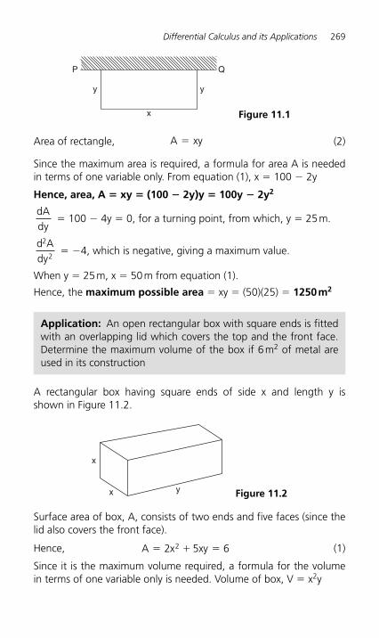
Differential Calculus and its Applications 269
Area of rectangle, A xy� (2)
Since the maximum area is required, a formula for area A is needed in terms of one variable only. From equation (1), x � 100 � 2y
Hence, area, A � xy � (100 � 2y)y � 100y � 2y 2
dAdy
� 100 � 4y � 0, for a turning point, from which, y � 25 m.
d Ady
2
2 � � 4, which is negative, giving a maximum value.
When y � 25 m, x � 50 m from equation (1).
Hence, the maximum possible area � xy � (50)(25) � 1250 m2
P Q
yy
x Figure 11.1
yx
x
Figure 11.2
Application: An open rectangular box with square ends is fitted with an overlapping lid which covers the top and the front face. Determine the maximum volume of the box if 6 m 2 of metal are used in its construction
A rectangular box having square ends of side x and length y is shown in Figure 11.2 .
Surface area of box, A, consists of two ends and five faces (since the lid also covers the front face).
Hence, A x xy� � �2 5 62 (1)
Since it is the maximum volume required, a formula for the volume in terms of one variable only is needed. Volume of box, V � x 2 y
270 Engineering Mathematics Pocket Book
From equation (1), yx
xx
��
� �6 2
565
25
2
x(2)
Hence, volume V � x 2 y � x 2 65
25
65
25
3
xx x x
� � �⎛⎝⎜⎜⎜
⎞⎠⎟⎟⎟⎟
dVdx
�
65
65
02
� �x for a maximum or minimum value.
Hence, 6 � 6x 2, giving x � 1 m (x � � 1 is not possible, and is thus neglected).
d Vdx
x.
2
2
125
��
When x � 1,d Vdx
2
2 is negative, giving a maximum
value.
From equation (2), when x � 1, y � 65
25
45
� �
Hence, the maximum volume of the box,
V � x 2 y � (1) 2
45
⎛⎝⎜⎜⎜
⎞⎠⎟⎟⎟⎟ �
45
m3
11.9 Tangents and normals
The equation of the tangent to a curve y � f(x) at the point (x1 , y 1 ) is given by:
y y m(x x )1 1� � �
where mdydx
� � gradient of the curve at (x 1 , y 1 ).
The equation of the normal to a curve at the point (x 1, y 1) is given by:
y y1m
(x x )1 1� � � �
Application: Find the equation of the tangent to the curve y � x 2 � x � 2 at the point (1, � 2)
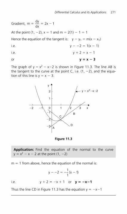
Differential Calculus and its Applications 271
Gradient, mdydx
x� � �2 1
At the point (1, � 2), x � 1 and m � 2(1) � 1 � 1
Hence the equation of the tangent is: y � y 1 � m(x � x 1 )
i.e. y � � 2 � 1(x � 1)
i.e. y � 2 � x � 1
or y � x � 3
The graph of y � x 2 � x �2 is shown in Figure 11.3 . The line AB is the tangent to the curve at the point C, i.e. (1, � 2), and the equa-tion of this line is y � x � 3.
1
y
B
D
C
A
x
1
2
2 30�1
�1
�2
�3
�2
y � x2�x�2
Figure 11.3
Application: Find the equation of the normal to the curve y � x 2 � x � 2 at the point (1, � 2)
m � 1 from above, hence the equation of the normal is:
y � � � � �211
1(x )
i.e. y � 2 � � x � 1 or y � � x � 1
Thus the line CD in Figure 11.3 has the equation y � � x � 1
272 Engineering Mathematics Pocket Book
11.10 Small changes using differentiation
If y is a function of x, i.e. y � f(x), and the approximate change in y corresponding to a small change δ x in x is required, then:
δδ
≈yx
dydx
and δ ≈ δ δ ≈ δydydx
x y f (x) x � or
Application: The time of swing T of a pendulum is given by T � k � , where � is a constant. Determine the percentage change in the time of swing if the length of the pendulum � changes from 32.1 cm to 32.0 cm
If T � k k� ��12 , then
dTd
kk
��
�� ��1
2 2
12
⎛⎝⎜⎜⎜
⎞⎠⎟⎟⎟⎟
Approximate change in T, δ t �
dTd
k�
δ δ��
��2
⎛
⎝⎜⎜⎜⎜
⎞
⎠⎟⎟⎟⎟
� k( ) (negative
20 1
�
⎛
⎝⎜⎜⎜⎜
⎞
⎠⎟⎟⎟⎟ � .
since decreases)�
Percentage error �approximate change in T
original value of T
⎛
⎝⎜⎜⎜⎜
⎞
⎠⎟⎟⎟⎟100%%
�
�
� ��
��
k( )
k% %
(
20 1
1000 12
100
0 12
�
� �
⎛
⎝⎜⎜⎜⎜
⎞
⎠⎟⎟⎟⎟ ⎛
⎝⎜⎜⎜
⎞⎠⎟⎟⎟⎟
..
.332 1
100. )
%⎛
⎝⎜⎜⎜⎜
⎞
⎠⎟⎟⎟⎟ � �0.156%
Hence, the change in the time of swing is a decrease of 0.156%
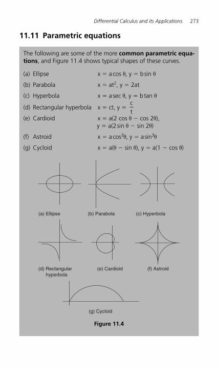
Differential Calculus and its Applications 273
11.11 Parametric equations
The following are some of the more common parametric equa-tions, and Figure 11.4 shows typical shapes of these curves.
(a) Ellipse x � a cos θ , y � b sin θ
(b) Parabola x � at 2 , y � 2at
(c) Hyperbola x � a sec θ , y � b tan θ
(d) Rectangular hyperbola x � ct, y � ct
(e) Cardioid x � a(2 cos θ � cos 2 θ ), y � a(2 sin θ � sin 2 θ )
(f) Astroid x � a cos 3 θ , y � a sin 3 θ
(g) Cycloid x � a( θ � sin θ ), y � a(1 � cos θ )
(a) Ellipse (c) Hyperbola
(e) Cardioid (f) Astroid
(g) Cycloid
(d) Rectangular hyperbola
(b) Parabola
Figure 11.4
274 Engineering Mathematics Pocket Book
x � 5 θ � 1, hence dxdθ
� 5
y � 2 θ ( θ � 1) � 2 θ 2 � 2 θ , hence dydθ
� 4 θ � 2 � 2(2 θ � 1)
From equation (1), dydx
� ��
dyddxd
( )θ
θ
θ2 2 15
or25
(2 1)θ �
Differentiation in parameters
When x and y are both functions of θ , then:
dydx
dyddxd
� θ
θ
(1)
and
d ydx
dd
dydx
dxd
2
2�
θ
θ
⎛⎝⎜⎜⎜
⎞⎠⎟⎟⎟⎟
(2)
Application: Given x � 5 θ � 1 and y � 2 θ ( θ � 1), determine dydx
in terms of θ .
Application: The parametric equations of a cycloid are x � 4( θ � sin θ ), y � 4(1 � cos θ ). Determine
(a)dydx
(b)d ydx
2
2
(a) x � 4( θ � sin θ ), hence dxdθ
� 4 � 4 cos θ � 4(1 � cos θ )
y � 4(1 � cos θ ), hence dydθ
� 4 sin θ
From equation (1), dydx
sin(1 cos )
� ��
�
dyddxd
( )θ
θ
θθ
44 1
sincos
θθ�
Differential Calculus and its Applications 275
(b) From equation (2),
d ydx
2
2�
�
��
� �ddθ
θθ
θ
θ θsincos
( cos )
( cos )(cos ) (si1
4 1
1⎛⎝⎜⎜⎜
⎞⎠⎟⎟⎟
nn )(sin )( cos )( cos )
cos cos sin( cos )
co
θ θθ
θ
θ θ θθ
14 1
4 1
2
2 2
3
�
�
�� �
��
ss (cos sin )( cos )
cos( cos )
( cos )(
θ θ θθ
θθ
θ
� �
��
��
� �
2 2
3
3
4 1
14 1
14 1
−
− ccos )θ 3�
�
�
14(1 cos )2θ
Application: When determining the surface tension of a liquid, the radius of curvature ρ , of part of
the surface is given by: ρ �
�12 3
2
2
dydx
d ydx
⎛⎝⎜⎜⎜
⎞⎠⎟⎟⎟⎟
⎡
⎣
⎢⎢⎢
⎤
⎦
⎥⎥⎥
Find the radius of curvature of the part of the surface having the parametric equations
x � 3t 2 , y � 6t at the point t � 2
x � 3t 2 , hence dxdt
� 6t and y � 6t, hence dydt
� 6
From equation (1),
dydx
dydtdxdt
t t� � �
66
1
From equation (2),
d ydt
ddt
dydx
dxdt
ddt t
t
ddt
t2
2
11
6 6� � �
�⎛⎝⎜⎜⎜
⎞⎠⎟⎟⎟⎟
⎛⎝⎜⎜⎜
⎞⎠⎟⎟⎟⎟ ( )
tttt t t
��
��
��2 2
36
1
61
6t =
276 Engineering Mathematics Pocket Book
Hence radius of curvature, ρ �
�
�
�1 11
2 3
2
2
2dydx
d ydx
t
⎛⎝⎜⎜⎜
⎞⎠⎟⎟⎟⎟
⎡
⎣
⎢⎢⎢
⎤
⎦
⎥⎥⎥
⎛⎝⎜⎜⎜
⎞⎠⎟⎟⎟⎟
⎡
⎣
⎢⎢⎢⎢
⎤
⎦
⎥⎥⎥
3
3
16�
t
When t � 2,
ρ �
�
�
�
�
� �
112
16 2
1 251
48
48 1 25
2 3
3
33
⎛⎝⎜⎜⎜
⎞⎠⎟⎟⎟⎟
⎡
⎣
⎢⎢⎢
⎤
⎦
⎥⎥⎥
−
( )
..
( )��67.08
11.12 Differentiating implicit functions
ddx
[f(y)]d
dy[f(y)]
dydx
� � (3)
Sometimes with equations involving, say, y and x, it is impossible to make y the subject of the formula. The equation is then called an implicit function and examples of such functions include y3 � 2x 2 � y 2 � x and sin y � x 2 � 2xy
Application: Differentiate u � sin 3t with respect to x
dudx
dudt
dtdx
ddt
( t)dtdx
� � � � �sin 3 3cos 3tdtdx
Application: Differentiate u � 4 ln 5y with respect to t
dudt
dudy
dydt
ddy
( ln y)dydt
� � � � �4 54y
dydt
⎛
⎝⎜⎜⎜⎜
⎞
⎠⎟⎟⎟⎟
Application: Determine ddx
(x y)2
Differential Calculus and its Applications 277
ddx
(x y) (x )ddx
(y) (y)ddx
(x ), by the product rule2 2 2� �
� �(x )
dydx
y( x), by using equation (3)2 1 2⎛⎝⎜⎜⎜
⎞⎠⎟⎟⎟⎟
� x2 dy
dx2xy�
Application: Determine ddx
yx
32
⎛⎝⎜⎜⎜
⎞⎠⎟⎟⎟⎟
ddx
yx
( x)ddx
( y) ( y)ddx
( x)
( x)
( x)dydx3
2
2 3 3 2
2
2 3
2
⎛⎝⎜⎜⎜
⎞⎠⎟⎟⎟⎟
⎛
��
�⎝⎝⎜⎜⎜
⎞⎠⎟⎟⎟⎟
⎛⎝⎜⎜⎜
⎞⎠⎟⎟⎟⎟
�
��
�
( y)( )
x
xdydx
y
x
3 2
4
6 6
4
2
2
32x
xdydx
y2
�
Application: Given 3x 2 � y 2 � 5x � y � 2 determine dydx
Differentiating term by term with respect to x gives:
ddx
( x )ddx
(y )ddx
( x)ddx
(y)ddx
( )3 5 22 2� � � �
i.e. 6x � 2ydydx
� 5 � 1 dydx
� 0 using equation (3) and standard derivatives.
Rearranging gives: (2y � 1) dydx
� 5 � 6x
from which, dydx
5 6x2y 1
��
�
Application: Determine the values of dydx
when x � 4 given that x 2 � y 2 � 25
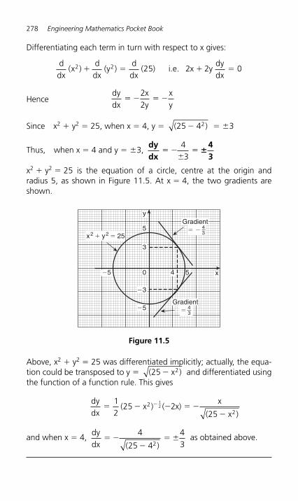
278 Engineering Mathematics Pocket Book
Differentiating each term in turn with respect to x gives:
ddx
ddx
(y )ddx
( ) i.e. x ydydx
( )x2 2 25 2 2 0� � � �
Hence dydx
xy
xy
� � � �22
Since x 2 � y 2 � 25, when x � 4, y � ( )25 42� � 3
Thus, when x � 4 and y � 3, dydx
43
� �
�43
�
x 2 � y 2 � 25 is the equation of a circle, centre at the origin and radius 5, as shown in Figure 11.5 . At x � 4, the two gradients are shown.
Gradient� � 4
3
Gradient� 4
3
y
5
3
0 4 5 x
�3
�5
�5
x2 � y2 � 25
Figure 11.5
Above, x 2 � y 2 � 25 was differentiated implicitly; actually, the equa-tion could be transposed to y � ( x )25 2� and differentiated using the function of a function rule. This gives
dydx
( x ) ( x)x
( x )� � � � �
�
�12
25 225
22
12
and when x � 4, dydx ( )
� ��
� 4
25 4
432
as obtained above.
Differential Calculus and its Applications 279
11.13 Differentiation of logarithmic functions
Logarithmic differentiation is achieved with knowledge of (i) the laws of logarithms, (ii) the differential coefficients of logarith-mic functions, and (iii) the differentiation of implicit functions.
(i) The laws of logarithms are: 1. log(A � B) � log A � log B
2. log AB
⎛⎝⎜⎜⎜
⎞⎠⎟⎟⎟⎟
� log A � log B
3. log A n � n log A
(ii) The differential coefficient of the logarithmic function ln x is given by:
ddx
(ln x)1x
�
More generally, it may be shown that:
ddx
[ln f(x)]f (x)f(x)
��
(4)
(iii) Differentiation of implicit functions is obtained using:
ddx
[f(y)]d
dy[f(y)]
dydx
� � (5)
Application: If y � ln(3x 2 � 2x � 1) determine dydx
If y � ln(3x 2 � 2x � 1) then dydx
6x 23x 2x 12
��
� �
Application: If y � ln(sin 3x) determine dydx
If y � ln(sin 3x) then dydx
3 cos 3xsin 3x
3 cot 3x� �
280 Engineering Mathematics Pocket Book
(i) Taking Napierian logarithms of both sides of the equation gives:
ln y � ln ( x) (x )
x (x )ln
( x) (x )x(x )
/
/
1 1
2
1 12
2 2 1 2
1 2
� �
��
� �
�
⎧⎨⎪⎪
⎩⎪⎪
⎫⎬⎪⎪
⎭⎪⎪
⎧⎨⎨⎪⎪⎩⎪⎪
⎫⎬⎪⎪⎭⎪⎪
(ii) Applying the laws of logarithms gives:
ln y � ln(1 � x) 2 � ln(x � 1) 1/2 � ln x � ln(x � 2) 1/2 by laws 1 and 2
i.e. ln y � 2 ln(1 � x) �
12
ln(x � 1) � ln x �
12
ln(x � 2) by law 3
(iii) Differentiating each term in turn with respect to x using equa-tions (4) and (5) gives:
1 21
12
11
12
2ydydx ( x) (x ) x (x )
��
��
� ��
(iv) Rearranging the equation to make dydx
the subject gives:
dydx
��
��
� ��
y( x) (x ) x (x )
21
12 1
1 12 2
⎧⎨⎪⎪⎩⎪⎪
⎫⎬⎪⎪⎭⎪⎪
(v) Substituting for y in terms of x gives:
dydx
(1 x) (x 1)x (x 2)
2(1 x)
12(x 1)
1x
12(x 2)
2�
� �
� ��
�� �
�
⎧⎨⎪⎪⎩⎪⎪
⎫⎬⎪⎪⎭⎭⎪⎪
Application: Differentiate y � ( x) (x )
x (x )
1 1
2
2� �
� with respect to x
Application: Determine dydx
given y � x x
Taking Napierian logarithms of both sides of y � x x gives:
ln y � ln x x � x ln x by law 3
Differential Calculus and its Applications 281
Differentiating both sides with respect to x gives:
1 11
ydydx
(x)x
(ln x)( ), using the product rule� �⎛⎝⎜⎜⎜
⎞⎠⎟⎟⎟⎟
i.e. 1y
dydx
� 1 � ln x from which, dydx
� y(1 � ln x)
i.e. dydx
� x x (1 � ln x)
Application: Determine the differential coefficient of
y � (x )x � 1 and evaluate dydx
when x � 2.
y � (x )x � 1 � (x � 1) 1/x since by the laws of indices: a amn mn�
Taking Napierian logarithms of both sides gives:
ln y � ln(x � 1) 1/x � 1x
ln(x � 1) by law 3
Differentiating each side with respect to x gives:
1 1 11
112y
dydx x x
[ln(x )]x
��
� ��⎛
⎝⎜⎜⎜
⎞⎠⎟⎟⎟⎟⎛⎝⎜⎜⎜
⎞⎠⎟⎟⎟⎟
⎛⎝⎜⎜⎜
⎞⎠⎟⎟⎟⎟⎟ by the product rule
Hence dydx
yx(x )
ln(x )x
��
��1
11
2
⎧⎨⎪⎪⎩⎪⎪
⎫⎬⎪⎪⎭⎪⎪
i.e. dydx
(x 1)x(x 1)
ln(x 1)x
x� ��
��12
⎧⎨⎪⎪⎩⎪⎪
⎫⎬⎪⎪⎭⎪⎪
When x � 2,dydx
� � � � �( )( )
ln( )1
12 1
14
112
02⎧⎨⎪⎪⎩⎪⎪
⎫⎬⎪⎪⎭⎪⎪
⎧⎨⎪⎪⎩⎪⎪
⎫⎬⎪⎪⎭⎪⎪
�112
11.14 Differentiation of inverse trigonometric functions
If y � 3x � 2, then by transposition, x � y � 2
3 . The function
x � y � 23
is called the inverse function of y � 3x � 2.
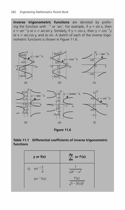
282 Engineering Mathematics Pocket Book
Inverse trigonometric functions are denoted by prefix-ing the function with � 1 or ‘ arc ’ . For example, if y � sin x, then x � sin � 1y or x � arc sin y. Similarly, if y � cos x, then y � cos � 1 y or x � arc cos y, and so on. A sketch of each of the inverse trigo-nometric functions is shown in Figure 11.6 .
Table 11.1 Differential coefficients of inverse trigonometric functions
y
y
y y
y � sin�1x
y � sec�1xy � cosec�1x
y � cot�1x
y � cos�1x
y � tan�1x
�1x�1
�1
A
3π/2 3π/2
0
�1 x0
(a) (b) (c)
(d) (e) (f)
�π/2
�3π/2�π
�π
�1x x�1 0 0
x0
�π/2
π/2
�π/2
�3π/2
�π
�π
ππ/2
y y
�1 x
π
ππ/2
π/2B
C
D
�π/2
3π/2π
π/2
�π/2
�3π/2
3π/2π
π/2
�1 0�π/2
�3π/2�π
Figure 11.6
y or f(x)
dydx
or f (x)�
(i) sin�1 xa
12 2a x�
sin ( )�1 f x f x
f x
�
�
( )
1 2[ ( )]
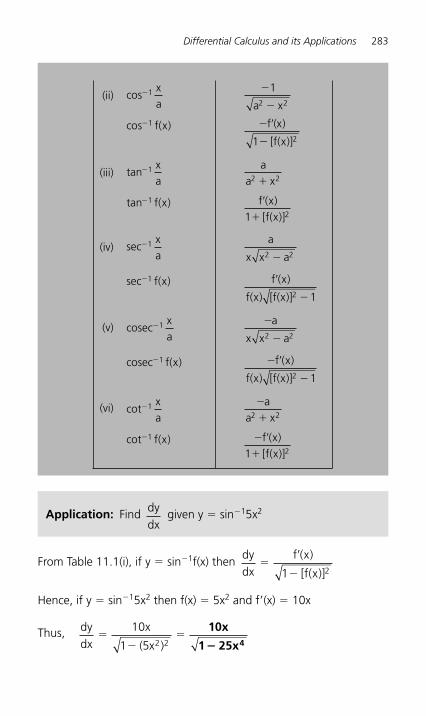
Differential Calculus and its Applications 283
From Table 11.1 (i), if y � sin � 1 f(x) then dydx f x
��
�
f x( )
[ ( )]1 2
Hence, if y � sin � 1 5x 2 then f(x) � 5x 2 and f � (x) � 10x
Thus, dydx
x
x�
��
10
1 5 2 2( )
10x
1 25x4�
(ii) cos�1 xa
�
�
12 2a x
cos ( )�1 f x � �
�
f x
f x
( )
1 2[ ( )]
(iii) tan�1 xa
aa x2 2�
tan ( )�1 f x f xf x
�
�
( )[ ( )]1 2
(iv) sec�1 xa
a
x x a2 2�
sec�1 f x( ) f x
f x f x
�
�
( )
( ) [ ( )]2 1
(v) cosec�1 xa
�
�
a
x x a2 2
cosec�1 f x( ) � �
�
f x
f x f x
( )
( ) [ ( )]2 1
(vi) cot�1 xa
�
�
aa x2 2
cot ( )�1 f x � �
�
f xf x( )
[ ( )]1 2
Application: Find dydx
given y � sin � 1 5x 2
284 Engineering Mathematics Pocket Book
Let u � cos � 1 3x then y � ln u
By the function of a function rule,
dydx
dydu
dudx u
ddx
(cos 3x)� � � � �1 1
��
��
13
3
1 31 2cos x x( )
⎧⎨⎪⎪⎪
⎩⎪⎪⎪
⎫⎬⎪⎪⎪
⎭⎪⎪⎪
i.e.d
dx[ln(cos 3x ]
3
1 9x cos 3x1
2 1�
��
�
�)
Application: Find the differential coefficient of y � ln(cos � 1 3x)
Application: Find dydt
given y � tan � 1 32t
Using the general form from Table 11.1 (iii),
f(t)t
t from which, f (t)t
� � � ���3
36
22
3
Hence,ddt
tanf (t)
f(t)t
t
� ��
��
�
�
12 2
3
2
2
31
6
13t
⎛⎝⎜⎜⎜
⎞⎠⎟⎟⎟ ⎛
⎝⎜⎜⎜
⎞⎠⎟⎟⎟⎟
[ ] ⎧⎧⎨⎪⎪⎪
⎩⎪⎪⎪
⎫⎬⎪⎪⎪
⎭⎪⎪⎪
��
�
6
93
4
4
tt
t
� ��
�6
93
4
4tt
t
⎛⎝⎜⎜⎜
⎞⎠⎟⎟⎟⎟⎛
⎝⎜⎜⎜⎜
⎞
⎠⎟⎟⎟⎟ �
�
6t 94
t
11.15 Differentiation of inverse hyperbolic functions
Inverse hyperbolic functions are denoted by prefixing the func-tion with � 1 or ‘ ar ’ . For example, if y � sinh x, then x � sinh � 1 y or x � ar sinh y. Similarly, if y � sech x, then x � sech � 1y or x � ar sech y, and so on. A sketch of each of the inverse hyper-bolic functions is shown in Figure 11.7 .
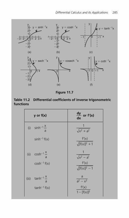
Differential Calculus and its Applications 285
Table 11.2 Differential coefficients of inverse trigonometric functions
y or f(x)
dydx
or f (x)�
(i) sinh�1 xa
12 2x a�
sinh�1 f x( ) f x
f x
�
�
( )
[ ( )]2 1
(ii) cosh�1 xa
12 1x a�
cosh ( )�1 f x f x
f x
�
�
( )
[ ( )]2 1
(iii) tanh�1 xa
aa x2 2�
tanh ( )�1 f x f xf x
�
�
( )[ ( )]1 2
y � sinh�1x
y � sech�1x
x
x x
xx
y y y
y � cosech�1x y � coth�1x
y � cosh�1x y � tanh�1x
(a) (b)
(d) (e) (f)
(c)
�2�3
�1 �1�2�3
123
�1 0
0 0 0
00
1 2 31
1
2 3�2 �2�1 �1
�1
�1
x�1
�3
123
y y y
�2�3
�1
123
Figure 11.7
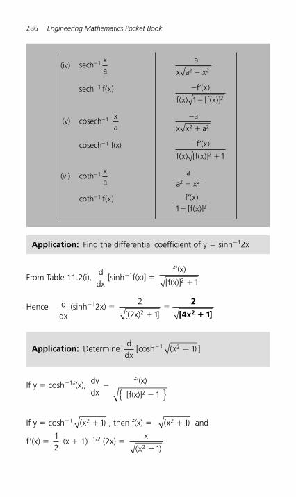
286 Engineering Mathematics Pocket Book
From Table 11.2 (i), ddx
[sinh � 1 f(x)] � f (x)
f(x)
�
�[ ]2 1
Hence ddx
(sinh � 1 2x) � 2
2 12[( x) ]��
2
4x 12[ ]�
Application: Find the differential coefficient of y � sinh � 1 2x
Application: Determine ddx
[cosh � 1 ( )x2 1+ ]
If y � cosh � 1 f(x), dydx
f (x)
f(x)�
�
�[ ]2 1{ }
If y � cosh � 1 ( )x2 1� , then f(x) � ( )x2 1� and
f� (x) � 12
(x � 1) � 1/2 (2x) � x
x )( 2 1�
(iv) sech�1 xa
�
�
a
x a x2 2
sech�1 f x( ) � �
�
f x
f x f x
( )
( ) [ ( )]1 2
(v) cosech xa
�1 �
�
a
x x a2 2
cosech f(x)�1 � �
�
f x
f x f x
( )
( ) [ ( )]2 1
(vi) coth�1 xa
aa x2 2�
coth ( )�1 f x f xf x
�
�
( )[ ( )]1 2
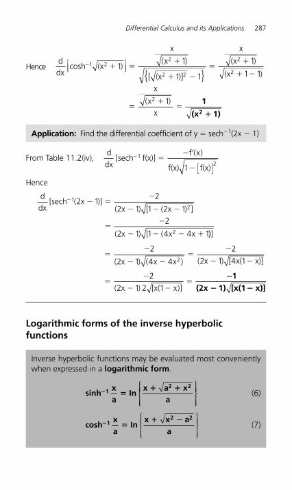
Differential Calculus and its Applications 287
Henceddx
cosh (x )
x
x
(x )]
x
(x )
(x )2� � �
�
� �
��
� �
12
2 2
2
21
1
1 1
1
1 1⎡⎣⎢
⎤⎦⎥ { }
( )
[
���
�
x
xx
( )2 1 1
(x 1)2 �
Application: Find the differential coefficient of y � sech � 1(2x � 1)
From Table 11.2 (iv),ddx
[sech f(x)]x
f(x) f(x)
� �� �
�
12
1
f ( )
[ ]
Hence
ddx
[sech ( )]( ) [ ( ) ]
( x ) [ ( x
� � ��
� � �
��
� � � �
12
2
2 12
2 1 1 2 1
2
2 1 1 4 4 1
xx x
x ))]
��
� ��
�
� �
2
2 1 4 4
2
2 1 4 12( x ) ( x x ( x ) [ x( x)])
��
� ��
2
2 1 2 1( ) [ ( )]x x x
�
� �
1(2x 1) [x(1 x)]
Logarithmic forms of the inverse hyperbolic functions
Inverse hyperbolic functions may be evaluated most conveniently when expressed in a logarithmic form.
sinhxa
Inx a x
a1
2 2� �
� �⎧⎨⎪⎪⎪
⎩⎪⎪⎪
⎫⎬⎪⎪⎪
⎭⎪⎪⎪
(6)
coshxa
Inx x a
a1
2 2� �
� �⎧⎨⎪⎪⎪
⎩⎪⎪⎪
⎫⎬⎪⎪⎪
⎭⎪⎪⎪
(7)
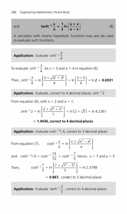
288 Engineering Mathematics Pocket Book
To evaluate sinh�1 34
let x � 3 and a � 4 in equation (6).
Then, sinh In In In� �� �
��
�12 23
43 4 3
43 5
4
⎧⎨⎪⎪⎪
⎩⎪⎪⎪
⎫⎬⎪⎪⎪
⎭⎪⎪⎪
⎛⎝⎜⎜⎜
⎞⎠⎟⎟⎟⎟ 22 � 0.6931
and tanhxa
12
lna xa x
1� ��
�
⎛⎝⎜⎜⎜
⎞⎠⎟⎟⎟⎟ (8)
A calculator with inverse hyperbolic functions may also be used to evaluate such functions.
Application: Evaluate sinh�1 34
From equation (6), with x � 2 and a � 1,
sinh In In In� �� �
� � �12 2
22 1 2
12 5 4 2361
⎧⎨⎪⎪⎪
⎩⎪⎪⎪
⎫⎬⎪⎪⎪
⎭⎪⎪⎪
( ) .
� 1.4436, correct to 4 decimal places
Application: Evaluate, correct to 4 decimal places, sinh � 1 2
Application: Evaluate cosh � 1 1.4, correct to 3 decimal places
From equation (7), cosh In� � �1
2 2xa
x x aa
⎧⎨⎪⎪⎪
⎩⎪⎪⎪
⎫⎬⎪⎪⎪
⎭⎪⎪⎪
and cosh � 1 1.4 � cosh � 1 1410
� cosh � 1 75
hence, x � 7 and a � 5
Then, cosh In In 2.3798
corr
� � �
�
12 27
57 7 5
5+ −⎧
⎨⎪⎪⎪
⎩⎪⎪⎪
⎫⎬⎪⎪⎪
⎭⎪⎪⎪
0 867. , eect to 3 decimal places
Application: Evaluate tanh�1 35
, correct to 4 decimal places
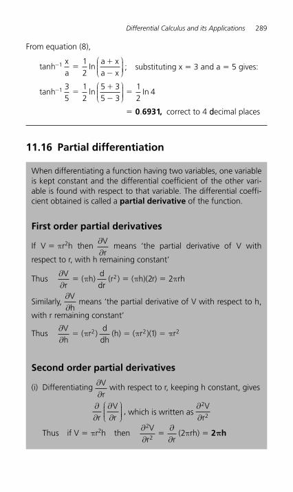
Differential Calculus and its Applications 289
From equation (8),
tanhxa
Ina xa x
� ��
�1 1
2
⎛⎝⎜⎜⎜
⎞⎠⎟⎟⎟⎟ ; substituting x � 3 and a � 5 gives:
tanh In
correct to 4
� ��
��
�
1 35
12
5 35 3
12
4ln
.
⎛⎝⎜⎜⎜
⎞⎠⎟⎟⎟⎟
0 6931, ddecimal places
11.16 Partial differentiation
When differentiating a function having two variables, one variable is kept constant and the differential coefficient of the other vari-able is found with respect to that variable. The differential coeffi-cient obtained is called a partial derivative of the function.
First order partial derivatives
If V � π r 2h then∂∂Vr
means ‘the partial derivative of V with
respect to r, with h remaining constant ’
Thus ∂∂
π π πVr
( h)ddr
(r ) ( h)( r) rh� � �2 2 2
Similarly, ∂∂Vh
means ‘the partial derivative of V with respect to h,
with r remaining constant ’
Thus ∂∂
π π πV
( r )d
dh(h) ( r )( ) r
h� � �2 2 21
Second order partial derivatives
(i) Differentiating ∂∂Vr
with respect to r, keeping h constant, gives
∂∂r
Vr
,∂∂
⎛⎝⎜⎜⎜
⎞⎠⎟⎟⎟⎟
which is written as
∂∂
2
2
Vr
Thus if V � π r2h then ∂
∂π
2
22
Vr r
( rh)∂
∂� � 2 hπ
290 Engineering Mathematics Pocket Book
(ii) Differentiating ∂∂Vh
with respect to h, keeping r constant, gives
∂∂h
Vh
,∂∂
⎛⎝⎜⎜⎜
⎞⎠⎟⎟⎟⎟ which is written as
∂2
2
Vh∂
Thus∂∂
∂∂
π2
22V
h h( r )� � 0
(iii) Differentiating ∂∂Vh
with respect to r, keeping h constant, gives
∂∂
∂∂rVh
,⎛⎝⎜⎜⎜
⎞⎠⎟⎟⎟⎟ which is written as
∂∂ ∂
2Vr h
Thus ∂∂ ∂
∂∂
∂∂
∂∂
π2
2Vr h r
Vh r
( r )� � �⎛⎝⎜⎜⎜
⎞⎠⎟⎟⎟⎟ 2 rπ
(iv) Differentiating ∂∂Vr
with respect to h, keeping r constant, gives
∂∂
∂∂hVr
⎛⎝⎜⎜⎜
⎞⎠⎟⎟⎟⎟ ,
which is written as
∂∂ ∂
2Vh r
Thus∂∂ ∂
∂∂
∂∂
∂∂
π2
2V
h r hVr h
( rh)� � �⎛⎝⎜⎜⎜
⎞⎠⎟⎟⎟⎟ 2 rπ
∂∂
∂∂
∂∂ ∂
2
2
2
2
2Vr
,V
h,
Vr h
and∂∂ ∂
2Vh r
are examples of second
order partial derivatives. It is seen from (iii) and (iv) that
∂∂ ∂
∂∂ ∂
2 2Vr h
Vh r
� and such a result is always true for continuous
functions.
Application: If Z � 5x4 � 2x 3 y 2 � 3y determine∂∂
Zx
and ∂∂
Zy
If Z � 5x 4 � 2x 3 y 2 � 3y
then ∂∂
Zx
ddx
ddx
ddx
� � �( x ) ( y ) (x ) ( y) ( )5 2 3 14 2 3
� � � �20 2 3 3 03 2x ( y )( x ) ( y)( )2 20x 6x y3 2 2�
Differential Calculus and its Applications 291
and∂∂
Zy
ddy
ddy
ddy
� � �( x ) ( ) ( x ) (y ) (y)5 1 2 34 3 2
� � � �0 2 2 33( x )( y) 4x y 33 �
Application: The time of oscillation, t, of a pendulum is given
by: tg
� 2πl
where l is the length of the pendulum and g the
free fall acceleration due to gravity. Find ∂∂tl and
∂∂
tg
To find ∂∂
t1
, g is kept constant.
t 1/2� � �22 2
πlg g
lg
lπ π⎛
⎝
⎜⎜⎜⎜⎜
⎞
⎠
⎟⎟⎟⎟⎟
⎛
⎝
⎜⎜⎜⎜⎜
⎞
⎠
⎟⎟⎟⎟⎟
Hence,∂∂tl g
ddl
lg
l� � �2 2 12
1 2 1 2π π⎛
⎝
⎜⎜⎜⎜⎜
⎞
⎠
⎟⎟⎟⎟⎟
⎛
⎝
⎜⎜⎜⎜⎜
⎞
⎠
⎟⎟⎟⎟⎟
⎛⎝
( )/ /⎜⎜⎜⎜⎞⎠⎟⎟⎟⎟
⎛
⎝
⎜⎜⎜⎜⎜
⎞
⎠
⎟⎟⎟⎟⎟
⎛
⎝⎜⎜⎜⎜
⎞
⎠⎟⎟⎟⎟� �
2 1
2
πg l
πlg
To find ∂∂
tg
, l is kept constant.
t g /� � � �2 2 2 1 2π π πlg
llg
l( )⎛
⎝⎜⎜⎜⎜
⎞
⎠⎟⎟⎟⎟⎟
( )
Hence
∂∂
π ππt
gl
lg l
l� � �
��
��22
22
3 23
( )⎛⎝⎜⎜⎜
⎞⎠⎟⎟⎟⎟
( )⎛
⎝
⎜⎜⎜⎜⎜
⎞
⎠
⎟⎟⎟⎟⎟⎟/
g
ll
g3� �π
lg3
Application: Given Z � 4x 2 y 3 � 2x 3 � 7y 2 find
(a)∂∂
2
2
Zx
(b) ∂∂
2
2
Zy
(c) ∂2Zx y∂ ∂
(d)∂
∂ ∂
2Zy x
(a)
∂∂
Zx
� �8 63xy x2
∂∂
∂∂
∂∂
∂∂
2
23 28 6
Zx x
Zx x
x� � � �⎛⎝⎜⎜⎜
⎞⎠⎟⎟⎟⎟ ( xy ) 8y 12x3 �
292 Engineering Mathematics Pocket Book
(b)
∂∂
Zy
� �12 142 2x y y
∂∂
∂∂
∂∂
∂∂
2
22 2 14
Zy y
Zy y
� � � �⎛
⎝⎜⎜⎜⎜
⎞
⎠⎟⎟⎟⎟
(12x y y) 24x 142y �
(c)
∂∂ ∂
∂∂
∂∂
∂∂
22 212 14
Zx y x
Zy x
� � � �⎛
⎝⎜⎜⎜⎜
⎞
⎠⎟⎟⎟⎟
( x y y) 24xy2
(d)
∂∂ ∂
∂∂
∂∂
∂∂
23 28 6
Zy x y
Zx y
� � � �⎛⎝⎜⎜⎜
⎞⎠⎟⎟⎟⎟ ( xy x ) 24xy2
11.17 Total differential
If Z � f(u, v, w, … ), then the total differential, dZ , is given by:
dZ � � � �∂∂
∂∂
∂∂
Zu
duZv
dvZw
dw ..... (9)
Application: If Z � f(u, v, w) and Z � 3u 2 � 2v � 4w 3 v 2 deter-mine the total differential dZ
Total differential, dZZu
du dv� � �∂∂
∂∂
∂∂
Zv
Zw
dw
∂∂
Zu
� 6u (i.e. v and w are kept constant)
∂∂
Zv
� �2 � 8w 3 v (i.e. u and w are kept constant)
∂∂
Zw
� 12w 2 v 2 (i.e. u and v are kept constant)
Hence, dZ � 6u du � (8vw 3 � 2)dv � (12v 2 w 2)dw
Differential Calculus and its Applications 293
11.18 Rates of change using partial differentiation
If Z � f(u, v, w, ...) and dudt
,
dvdt
,
dwdt
....., denote the rate of
change of u, v, w, ….respectively, then the rate of change of Z, dZdt
, is given by:
dZdt
Zu
dudt
Zv
dvdt
Zw
dwdt
� � � �∂∂
∂∂
∂∂
.. (9)
Application: If the height of a right circular cone is increasing at 3 mm/s and its radius is decreasing at 2 mm/s, find the rate at which the volume is changing (in cm 3/s) when the height is 3.2 cm and the radius is 1.5 cm.
Volume of a right circular cone, V r h�13
2π
Using equation (9), the rate of change of volume,
dVdt
Vr
drdt
Vh
dhdt
� �∂∂
∂∂
∂∂
πVr
rh�23
and ∂∂
πVh
r�13
2
Since the height is increasing at 3 mm/s, i.e. 0.3 cm/s, thendhdt
�
�0.3 and since the radius is decreasing at 2 mm/s, i.e. 0.2 cm/s, then drdt
� �0.2
Hence, dVdt
rh r� � � � ��2
30 2
13
0 30 43
2π π⎛⎝⎜⎜⎜
⎞⎠⎟⎟⎟⎟
⎛⎝⎜⎜⎜
⎞⎠⎟⎟⎟⎟( . ) ( . )
.πrhh r� 0 1 2. π
However, h � 3.2 cm and r � 1.5 cm.
Hence dVdt
( )( ) ( ) ( )��
�0 43
1 5 3 2 0 1 1 5 2.. . . .π π
� �2.011 � 0.707 � �1.304 cm 3 /s
Thus, the rate of change of volume is 1.30 cm 3 /s decreasing
294 Engineering Mathematics Pocket Book
11.19 Small changes using partial differentiation
If Z � f(u, v, w, …) and δu, δv, δw, … denote small changes in u, v, w, … respectively, then the corresponding approximate change δ Z in Z is given by:
δ ≈∂∂
δ∂∂
δ∂∂
δZZu
uZv
vZw
w� � � ..... (10)
Application: If the modulus of rigidity G � (R 4 θ)/L, where R is the radius, θ the angle of twist and L the length, find the approximate percentage error in G when R is increased by 2%, θ is reduced by 5% and L is increased by 4%
From equation (10), δ∂∂
δ∂∂θ
δθ∂∂
δGGR
RG G
LL� � �
Since GRL
,GR
RL
,G R
L� � �
4 3 44θ ∂∂
θ ∂∂θ
and ∂∂
θGL
RL
�� 4
2
Since R is increased by 2%, δ R �
2100
R � 0.02 R
Similarly, δ θ � �0.05 θ and δ L � 0.04 L
Hence δ θG ( R) ( )�4
0 02 0 053 4 4
2
RL
RL
RL
θ θ⎛
⎝⎜⎜⎜⎜
⎞
⎠⎟⎟⎟⎟
⎛
⎝⎜⎜⎜⎜
⎞
⎠⎟⎟⎟⎟. .� � � �
⎛⎛
⎝⎜⎜⎜⎜
⎞
⎠⎟⎟⎟⎟ ( L)0 04.
� �
�
RL
[ ]RL
i.e. G G
4 40 08 0 05 0 04 0 01
1100
θ θ
δ
. . . .� � �
�
Hence the approximate percentage error in G is a 1% decrease.
Application: If the second moment of area I of a rectangle is given
by I � bl3
3, find the approximate error in the calculated value of l,
if b and l are measured as 40 mm and 90 mm respectively and the measurement errors are –5 mm in b and � 8 mm in l.
Differential Calculus and its Applications 295
Using equation (10), the approximate error in I, δ I � ∂∂
Ib
δ b � ∂∂
II
δ l
∂∂
∂∂
I ll
ll
band
I bb� � �
3 22
33
3 δ b � � 5 mm and δ l � � 8 mm
Hence δ I � l3
3
⎛
⎝⎜⎜⎜⎜
⎞
⎠⎟⎟⎟⎟ ( � 5) � (bl 2 )( � 8)
Since b � 40 mm and l � 90 mm then
δ I � 903
3⎛
⎝⎜⎜⎜⎜
⎞
⎠⎟⎟⎟⎟ ( � 5) � 40(90) 2 (8)
� � 1,215,000 � 2,592,000
� 1,377,000 mm 4 � 137.7 cm 4
Hence, the approximate error in the calculated value of I is a 137.7 cm 4 increase.
11.20 Maxima, minima and saddle points of functions of two variables
Procedure to determine maxima, minima and saddle points for functions of two variables
Given z � f(x, y):
(i) determine ∂∂
zx and
∂∂
zy
(ii) for stationary points, ∂∂
zx
� 0 and ∂∂
zy
� 0,
(iii) solve the simultaneous equations∂∂
zx
� 0 and∂∂
zy
� 0 for x
and y, which gives the co-ordinates of the stationary points,
(iv) determine ∂∂
∂∂
∂∂ ∂
2
2
2
2
2zx
,z
yand
zx y
296 Engineering Mathematics Pocket Book
Following the above procedure:
(i) ∂∂
zx
� 2(x � 1) and ∂∂
zy
� 2(y � 2)
(ii) 2 1 0(x )� � (1)
2 2 0(y )� � (2)
(iii) From equations (1) and (2), x � 1 and y � 2, thus the only s tationary point exists at (1, 2)
(iv) Since ∂∂
zx
� 2(x � 1) � 2x � 2, ∂∂
2
2
zx
� 2
and since ∂∂
zy
� 2(y � 2) � 2y � 4, ∂∂
2
2
zy
� 2
(v) for each of the co-ordinates of the stationary points,
substitute values of x and y into∂∂
∂∂
∂∂ ∂
2
2
2
2
2zx
,z
yand
zx y
and
evaluate each,
(vi) evaluate ∂
∂ ∂
2 2z
x y
⎛
⎝⎜⎜⎜⎜
⎞
⎠⎟⎟⎟⎟
for each stationary point,
(vii) substitute the values of∂∂
∂∂
∂∂ ∂
2
2
2
2
2zx
,z
yand
zx y
into the equation
Δ∂
∂ ∂∂∂
∂∂
� �2 2 2
2
2
2
zx y
zx
zy
⎛
⎝⎜⎜⎜⎜
⎞
⎠⎟⎟⎟⎟
⎛
⎝⎜⎜⎜⎜
⎞
⎠⎟⎟⎟⎟⎛
⎝⎜⎜⎜⎜
⎞
⎠⎟⎟⎟⎟⎟
and evaluate,
(viii) (a) if Δ > 0 then the stationary point is a saddle point
(b) if Δ < 0 and∂∂
<2
2
zx
0, then the stationary point is a
maximum point , and
(c) if Δ < 0 and∂∂
<2
2
zx
0, then the stationary point is a
minimum point
Application: Determine the co-ordinates of the stationary point and its nature for the function z � (x � 1) 2 � (y � 2) 2
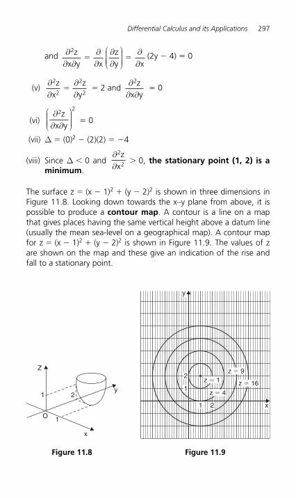
Differential Calculus and its Applications 297
and ∂∂ ∂
∂∂
∂∂
∂∂
2zx y x
zy x
� �⎛
⎝⎜⎜⎜⎜
⎞
⎠⎟⎟⎟⎟
(2y � 4) � 0
(v) ∂∂
∂∂
2
2
2
2
zx
zy
� � 2 and ∂
∂ ∂
2zx y
� 0
(vi) ∂
∂ ∂
2 2z
x y
⎛
⎝⎜⎜⎜⎜
⎞
⎠⎟⎟⎟⎟ � 0
(vii) Δ � (0) 2 � (2)(2) � � 4
(viii) Since Δ 0 and∂∂
2
2
zx
0, the stationary point (1, 2) is a minimum.
The surface z � (x � 1) 2 � (y � 2) 2 is shown in three dimensions in Figure 11.8 . Looking down towards the x–y plane from above, it is possible to produce a contour map. A contour is a line on a map that gives places having the same vertical height above a datum line (usually the mean sea-level on a geographical map). A contour map for z � (x � 1) 2 � (y � 2) 2 is shown in Figure 11.9 . The values of z are shown on the map and these give an indication of the rise and fall to a stationary point.
1 2
1O
Z
x
y
Figure 11.8
y
x21
1
2z � 1
z � 4
z � 9
z � 16
Figure 11.9
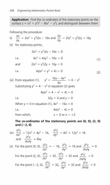
298 Engineering Mathematics Pocket Book
Following the procedure:
(i) ∂∂
zx
� 2(x 2 � y 2 )2x � 16x and ∂∂
zy
� 2(x 2 � y 2 )2y � 1 6y
(ii) for stationary points,
i.e.
2 2 16
4 4 16
2 2
3 2
(x y ) x x 0
x xy x 0
� � �
� � � (1)
and 2(x 2 � y 2 )2y � 16y � 0
i.e. 4y(x y ) 0 2 2� � �4 (2)
(iii) From equation (1), y 2 � 16 44
3x xx
� � 4 � x 2
Substituting y 2 � 4 � x 2 in equation (2) gives
4y(x 2 � 4 � x 2 � 4) � 0
i.e. 32y � 0 and y � 0
When y � 0 in equation (1), 4x 3 � 16x � 0
i.e. 4x(x2 � 4) � 0
from which, x � 0 or x � 2
The co-ordinates of the stationary points are (0, 0), (2, 0) and ( � 2, 0)
(iv) ∂∂
2
2
zx
� 12x 2 � 4y 2 � 16,∂∂
2
2
zy
� 4x 2 � 12y 2 � 16
and∂
∂ ∂
2
x yz
� 8xy
(v) For the point (0, 0), ∂∂
2
2
zx
� � 16, ∂∂
2
2
zy
� 16 and ∂∂ ∂
2zx y
� 0
For the point (2, 0), ∂∂
2
2
zx
� 32, ∂∂
2
2
zy
� 32 and ∂∂ ∂
2zx y
� 0
For the point ( � 2, 0), ∂∂
2zx2
� 32, ∂∂
2
2
zy
� 32 and ∂
∂ ∂
2zx y
� 0
Application: Find the co-ordinates of the stationary points on the surface z � (x2 � y2)2 � 8(x2 � y2), and distinguish between them
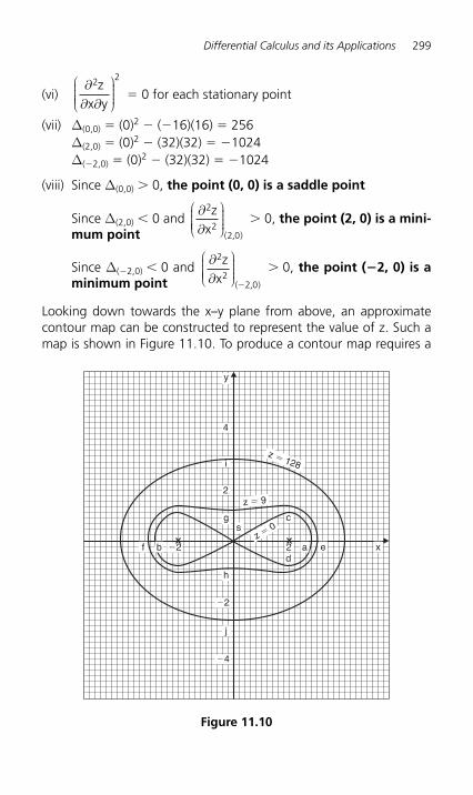
Differential Calculus and its Applications 299
(vi) ∂
∂ ∂
2 2z
x y
⎛
⎝⎜⎜⎜⎜
⎞
⎠⎟⎟⎟⎟ � 0 for each stationary point
(vii) Δ (0,0) � (0) 2 � ( � 16)(16) � 256 Δ (2,0) � (0) 2 � (32)(32) � � 1024 Δ (� 2,0) � (0) 2 � (32)(32) � � 1024
(viii) Since Δ (0,0) 0, the point (0, 0) is a saddle point
Since Δ (2,0) 0 and∂∂
2
22 0
zx ( , )
⎛
⎝⎜⎜⎜⎜
⎞
⎠⎟⎟⎟⎟
0, the point (2, 0) is a mini-mum point
Since Δ (� 2,0) 0 and ∂∂
2
22 0
zx ( , )
⎛
⎝⎜⎜⎜⎜
⎞
⎠⎟⎟⎟⎟
�
0, the point ( �2, 0) is a minimum point
Looking down towards the x–y plane from above, an approximate contour map can be constructed to represent the value of z. Such a map is shown in Figure 11.10 . To produce a contour map requires a
y
g
b ad
c
ez � 0
z � 9
z � 128
xf
h
j
�2
�2
�4
s
i
4
2
2
Figure 11.10
300 Engineering Mathematics Pocket Book
large number of x–y co-ordinates to be chosen and the values of z at each co-ordinate calculated. Here are a few examples of points used to construct the contour map.
When z � 0 , 0 � (x 2 � y 2 ) 2 � 8(x 2 � y 2 )
In addition, when, say, y � 0 (i.e. on the x-axis)
0 � x 4 � 8x 2 i.e. x 2 (x 2 � 8) � 0
from which, x � 0 or x � 8
Hence the contour z � 0 crosses the x-axis at 0 and 8 , i.e. at co-ordinates (0, 0), (2.83, 0) and ( �2.83, 0) shown as points S, a and b respectively.
When z � 0 and x � 2 then 0 � (4 � y 2 ) 2 � 8(4 � y 2 )
i.e. 0 � 16 � 8y 2 � y 4 � 32 � 8y 2
i.e. 0 � y 4 � 16y 2 � 16
Let y 2 � p, then p 2 � 16p � 16 � 0
and p( )( )
�� �
�� 16 16 4 1 16
216 17 89
2
2 − .
� 0.945 or � 16.945
Hence y � p � ( )0 945. or ( )�16 945. � 0.97 or complex roots
Hence the z � 0 contour passes through the co-ordinates (2, 0.97) and (2, � 0.97) shown as c and d in Figure 11.10 .
Similarly, for the z � 9 contour, when y � 0,
9 � (x 2 � 0 2 ) 2 � 8(x 2 � 0 2 )
i.e. 9 � x 4 � 8x 2
i.e. x 4 � 8x 2 � 9 � 0
Hence (x 2 � 9)(x 2 � 1) � 0 from which, x � 3 or complex roots
Thus the z � 9 contour passes through (3, 0) and ( �3, 0), shown as e and f in Figure 11.10.
If z � 9 and x � 0, 9 � y 4 � 8y 2
i.e. y 4 � 8y 2 � 9 � 0
i.e. (y 2 � 9)(y 2 � 1) � 0
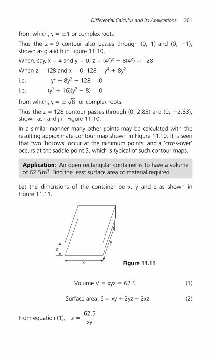
Differential Calculus and its Applications 301
from which, y � 1 or complex roots
Thus the z � 9 contour also passes through (0, 1) and (0, � 1), shown as g and h in Figure 11.10 .
When, say, x � 4 and y � 0, z � (4 2 ) 2 � 8(4 2 ) � 128
When z � 128 and x � 0, 128 � y 4 � 8y 2
i.e. y 4 � 8y 2 � 128 � 0
i.e. (y 2 � 16)(y 2 � 8) � 0
from which, y � 8 or complex roots
Thus the z � 128 contour passes through (0, 2.83) and (0, � 2.83), shown as i and j in Figure 11.10 .
In a similar manner many other points may be calculated with the resulting approximate contour map shown in Figure 11.10 . It is seen that two ‘ hollows ’ occur at the minimum points, and a ‘ cross-over ’ occurs at the saddle point S, which is typical of such contour maps.
y
x
z
Figure 11.11
Application: An open rectangular container is to have a volume of 62.5 m 3 . Find the least surface area of material required
Let the dimensions of the container be x, y and z as shown in Figure 11.11 .
Volume V xyz 62.5� � (1)
Surface area, S xy 2yz 2xz� � � (2)
From equation (1), z �
62 5.xy
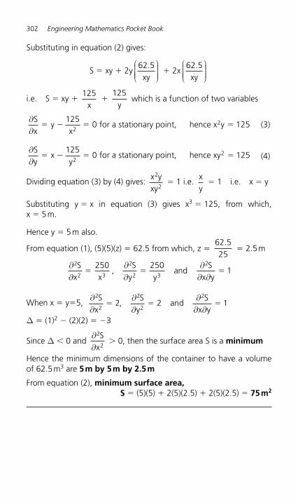
302 Engineering Mathematics Pocket Book
Substituting in equation (2) gives:
S � xy � 2y 62 5.xy
⎛
⎝⎜⎜⎜⎜
⎞
⎠⎟⎟⎟⎟
� 2x 62 5.xy
⎛
⎝⎜⎜⎜⎜
⎞
⎠⎟⎟⎟⎟
i.e. S � xy � 125
x �
125y
which is a function of two variables
∂∂
Sx
yx
for a stationary point, hence x y� � � �125
0 1252
2 (3)
∂∂
Sy
xy
for a stationary point, hence xy� � � �125
0 1252
2 (4)
Dividing equation (3) by (4) gives: x yxy
2
2 � 1 i.e.
xy
� 1 i.e. x � y
Substituting y � x in equation (3) gives x 3 � 125, from which, x � 5 m.
Hence y � 5 m also.
From equation (1), (5)(5)(z) � 62.5 from which, z � 62 525
. � 2.5 m
∂∂
∂∂
∂∂ ∂
2
2 3
2
2 3
2250 2501
Sx x
,S
y yand
Sx y
� � �
When x � y �5,∂∂
∂∂
∂∂ ∂
2
2
2
2
22 2 1
Sx
,S
yand
Sx y
� � �
Δ � (1) 2 � (2)(2) � � 3
Since Δ 0 and ∂∂
2
2
Sx
0, then the surface area S is a minimum
Hence the minimum dimensions of the container to have a volume of 62.5 m 3 are 5 m by 5 m by 2.5 m
From equation (2), minimum surface area, S � (5)(5) � 2(5)(2.5) � 2(5)(2.5) � 75 m 2
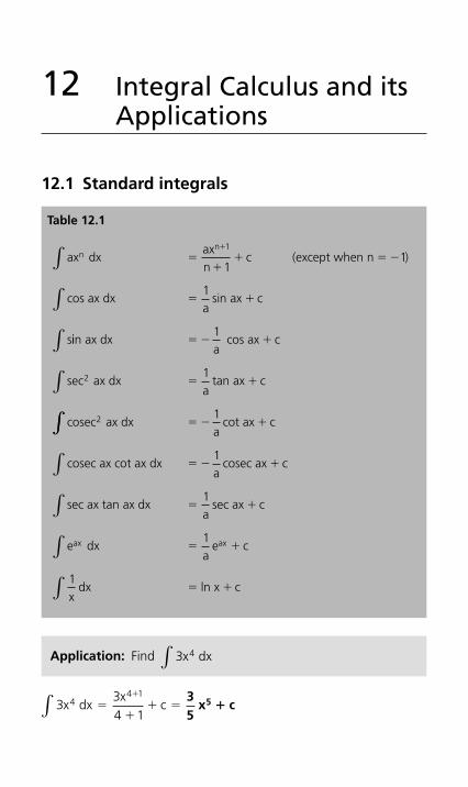
12 Integral Calculus and its Applications
12.1 Standard integrals
Application: Find 3 4x dx∫
Table 12.1
ax dxaxn
c (except when n )
cos ax dxa
sin ax c
s
nn
∫
∫
��
� � �
� �
�1
11
1
iin ax dxa
cos ax c
sec ax dxa
tan ax c
cosec ax dx
2
2
∫
∫
� � �
� �
1
1
∫∫
∫
� � �
� � �
1
1
acot ax c
cosec ax cot ax dxa
cosec ax c
sec ax tan ax dx sec ax c
e dxa
e c
1x
dx ln x c
ax ax
∫
∫
∫
� �
� �
� �
1
1
a
334 1
44 1
x dxx
c∫ ��
� �� 3
5x c5 �
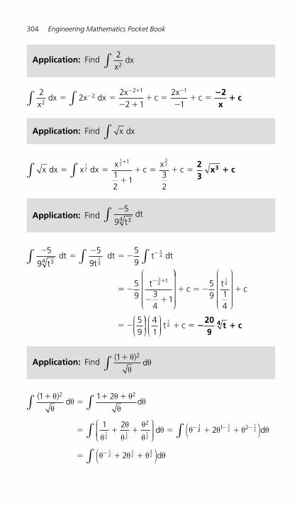
304 Engineering Mathematics Pocket Book
22
22 1
212
22 1 1
xdx x dx
xc
xc� �
� �� �
�� ��
� � �
∫∫�
�2
xc
Application: Find 22x
dx∫
Application: Find x dx∫
x dx x dxx
cx
c∫ ∫� �
�
� � � ��
12
12
321
12
132
23
x c3 �
��
�� �
� �
� �
�
� �
5
9
5
9
59
59 3
41
34
1
34
34
34
t dt
t dt t dt
t
∫ ∫ ∫⎛
⎝
⎜⎜⎜⎜⎜⎜⎜⎜⎜
⎞⎞
⎠
⎟⎟⎟⎟⎟⎟⎟⎟⎟⎟
⎛
⎝
⎜⎜⎜⎜⎜⎜⎜⎜⎜
⎞
⎠
⎟⎟⎟⎟⎟⎟⎟⎟⎟⎟
⎛⎝⎜⎜⎜
� � � �
� �
ct
c59 1
4
59
14
⎞⎞⎠⎟⎟⎟⎟⎛⎝⎜⎜⎜
⎞⎠⎟⎟⎟⎟
41
14t c� � � �
209
t c4
Application: Find �5
9 34 tdt∫
Application: Find ( )d
1 2� θθ
θ∫
( )d d
d
1 1 2
1 2
2 2
2
12
12
12
1
��
� �
� � � � �
θθ
θθ θθ
θ
θ
θ
θ
θ
θθ θ
∫ ∫
∫⎛
⎝⎜⎜⎜⎜
⎞
⎠⎟⎟⎟⎟
2212
12
12
12
32
2
2
1 2� �
� � �
� �
�
θ θ θ
θ θ θ θ
( )
( )
∫
∫
d
d
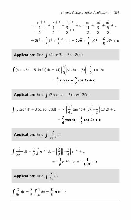
Integral Calculus and its Applications 305
�
� �
�
�
�
�
� � � � �
�
� � � �θ θ θ θ θ θ12
12
32
12
32
521 1 1
12
1
212
132
112
232
52
2
c c
θθ θ θ12
32
52
43
25
� � � �c 243
25
c3 5θ θ θ� � �
Application: Find ( x x)dx4 3 5 2cos sin�∫
( cos sin sin4 3 5 2 413
3 512
x x) dx ( ) x ( )� � � �∫⎛⎝⎜⎜⎜
⎞⎠⎟⎟⎟⎟
⎛⎝⎜⎜⎜
⎞⎠⎟⎟⎟⎟ ccos 2x
�43
sin 3x52
cos 2x c� �
Application: Find ( sec7 4 3 22 2t cosec t)dt�∫
( t cosec t)dt ( ) t ( )7 4 3 2 714
4 312
2 2sec tan� � � �∫⎛⎝⎜⎜⎜
⎞⎠⎟⎟⎟⎟
⎛⎝⎜⎜⎜
⎞⎠⎟⎟⎟⎟⎟ cot t c2 �
�74
tan 4t32
cot 2t c� �
Application: Find 2
3 4edt
t∫
23
23
23
14
16
44 4
edt e dt e c
e
tt t� � � �
� �
� �
�
∫∫⎛⎝⎜⎜⎜
⎞⎠⎟⎟⎟⎟⎛⎝⎜⎜⎜
⎞⎠⎟⎟⎟⎟
44t c� � � �1
6ec
4t
Application: Find 35x
dx∫
35
35
1x
dxx
dx∫ ∫� �35
ln x c�

306 Engineering Mathematics Pocket Book
Definite Integrals
Application: Evaluate ( x )dx4 22
3�
�∫
( x ) dx xx
( ) ( )4 43
4 333
4 222
3 3
2
3 3� � � � � � � �
��
∫⎡
⎣⎢⎢
⎤
⎦⎥⎥
⎛
⎝⎜⎜⎜⎜
⎞
⎠⎟⎟⎟⎟
(( )
( ) ( )
�
� � � � ��
� � �
23
12 9 88
33 5
13
3⎛
⎝⎜⎜⎜⎜
⎞
⎠⎟⎟⎟⎟
⎛⎝⎜⎜⎜
⎞⎠⎟⎟⎟⎟
⎛⎝⎜⎜⎜
⎞⎞⎠⎟⎟⎟⎟ � 8
13
Application: Evaluate 3 20
2sin x dx
π/
∫
3 2 312
232
22
0
2
sin ( ) cos cosx dx x x0
//
ππ
∫⎛⎝⎜⎜⎜
⎞⎠⎟⎟⎟
⎡
⎣⎢⎢
⎤
⎦⎥⎥
⎡
⎣� � � �⎢⎢
⎢⎤
⎦⎥⎥
⎛⎝⎜⎜⎜
⎞⎠⎟⎟⎟
⎧⎨⎪⎪⎩⎪⎪
⎫⎬⎪⎪⎭⎪⎪
⎧⎨
0
2
32
22
32
2 0
π
π
/
� � � �cos cos ( )⎪⎪⎪⎩⎪⎪
⎫⎬⎪⎪⎭⎪⎪
⎧⎨⎪⎪⎩⎪⎪
⎫⎬⎪⎪⎭⎪⎪
⎧⎨⎪⎪⎩⎪⎪
⎫⎬⎪⎪⎭⎪⎪
� � � � � �32
132
13
( ) ( )22
32
� � 3
Application: Evaluate 4 31
2cos t dt∫
4 3 413
343
31
2
1
2cos sin sint dt ( )� �
⎛⎝⎜⎜⎜
⎞⎠⎟⎟⎟⎟
⎡
⎣⎢⎢
⎤
⎦⎥⎥
⎡
⎣⎢⎢
⎤
⎦⎥∫ t t⎥⎥
⎧⎨⎪⎪⎩⎪⎪
⎫⎬⎪⎪⎭⎪⎪
⎧⎨⎪⎪⎩⎪⎪
⎫⎬⎪⎪⎭⎪⎪1
243
643
3� �sin sin
(Note that limits of trigonometric functions are always expressed in radians, thus, for example, sin 6 means the sine of 6 radians � � 0.279415..)
Hence, 4 343
0 27941543
0 1411201
2cos . ..) . ..)t dt ( (∫
⎧⎨⎪⎪⎩⎪⎪
⎫⎬⎪⎪⎭⎪⎪
⎧⎨� � �⎪⎪⎪⎩⎪⎪
⎫⎬⎪⎪⎭⎪⎪
� � � �( ) ( )0 37255 0 18816. . �0.5607
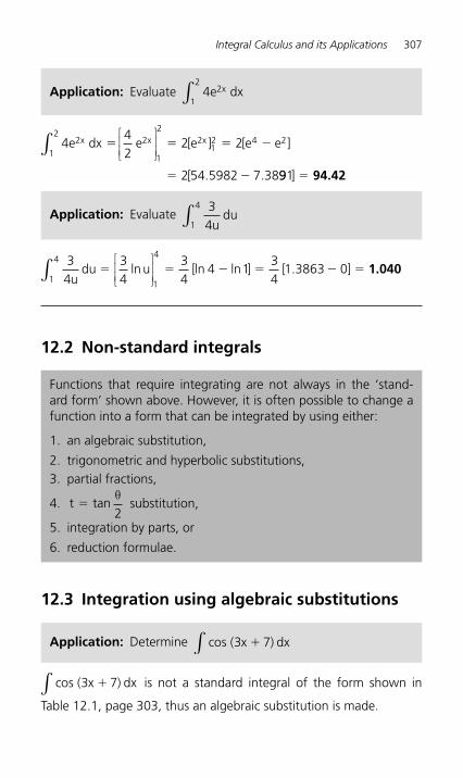
Integral Calculus and its Applications 307
442
2 2
2 54 5982 7 38
21
22
1
22
12 4 2e dx e e e ex x x� � � �
� �
∫⎡
⎣⎢⎢
⎤
⎦⎥⎥
[ ] [ ]
[ . . 991] � 94.42
Application: Evaluate 4 21
2e dxx∫
Application: Evaluate 341
4
udu∫
34
34
34
4 134
1 3863 01
4
1
4
udu ln u ln ln∫
⎡
⎣⎢⎢
⎤
⎦⎥⎥
� � � � � �[ ] [ . ] 1.040
12.2 Non-standard integrals
Functions that require integrating are not always in the ‘ stand-ard form ’ shown above. However, it is often possible to change a function into a form that can be integrated by using either:
1. an algebraic substitution,
2. trigonometric and hyperbolic substitutions, 3. partial fractions,
4. t tan�θ2
substitution,
5. integration by parts, or
6. reduction formulae.
12.3 Integration using algebraic substitutions
Application: Determine cos ( x ) dx3 7�∫
cos ( x ) dx3 7�∫ is not a standard integral of the form shown in
Table 12.1 , page 303, thus an algebraic substitution is made.
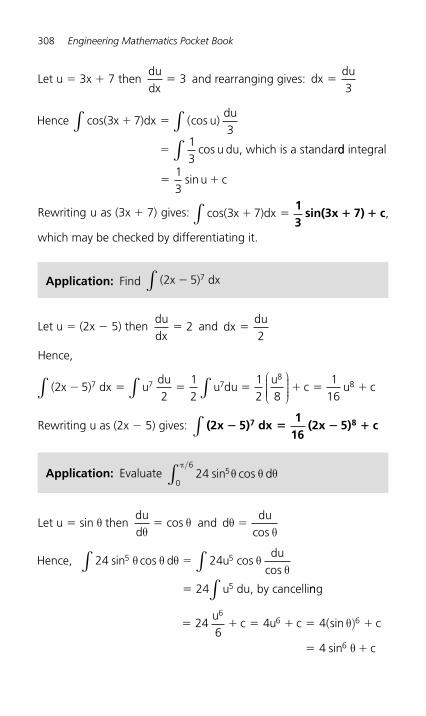
308 Engineering Mathematics Pocket Book
Let u � 3x � 7 then dudx
� 3 and rearranging gives: dxdu
�3
Hence cos( x )dx ( u)du
u du, which is a standar
3 73
13
� �
�
∫ ∫
∫
cos
cos dd integral
� �
13
sin u c
Rewriting u as (3x � 7) gives: cos( x )dx ,3 7� �13
sin(3x 7) c� �∫ which may be checked by differentiating it.
Application: Find ( x ) dx2 5 7�∫
Let u � (2x � 5) then dudx
� 2 and dxdu
�2
Hence,
( x ) dx udu
u duu
c u c2 52
12
12 8
116
7 7 78
8� � � � � � �∫ ∫∫⎛
⎝⎜⎜⎜⎜
⎞
⎠⎟⎟⎟⎟
Rewriting u as (2x � 5) gives: (2x 5) dx1
16(2x 5) c7 8� � � �∫
Application: Evaluate 24 50
6sin cos
π/θ θ θ∫ d
Let u � sin θ then dudθ
θ� cos and ddu
cosθ �
θ
Hence, d udu
u du, by cancelli
24 24
24
5 5
5
sin cos coscos
θ θ θ θθ∫ ∫
∫
�
� nng
� � � � � �
� �
246
4 4
4
66 6
6
uc u c ( c
c
sin
sin
θ)
θ
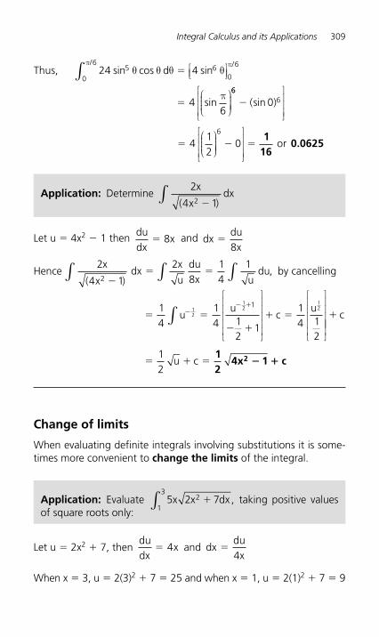
Integral Calculus and its Applications 309
Thus, d
sin
/ /24 4
46
50
66
0
6sin cos sin
π πθ θ θ θ
π
∫ ⎡⎣⎢
⎤⎦⎥
⎛⎝⎜⎜⎜
⎞⎠⎟⎟⎟⎟
�
�66
60� ( )sin⎡
⎣
⎢⎢⎢
⎤
⎦
⎥⎥⎥
� � �412
06⎛
⎝⎜⎜⎜
⎞⎠⎟⎟⎟⎟
⎡
⎣
⎢⎢⎢
⎤
⎦
⎥⎥⎥
116
0.0625or
Application: Determine 2
4 12
x
( x )dx
�∫
Let u � 4x 2 � 1 then dudx
x� 8 and dxdu
x�
8
Hence 2
4 1
28
14
12
x
( x ) dx
x
u
dux u
du�
� �∫ ∫ ∫ , by cancelling
� �
� �
� ��� �1
414 1
21
14 1
2
12
12
121
uu
cu
∫⎡
⎣
⎢⎢⎢⎢⎢
⎤
⎦
⎥⎥⎥⎥⎥
⎡
⎣
⎢⎢⎢⎢⎢
⎤
⎦
⎥⎥⎥⎥⎥⎥
� c
� � �12
u c12
4x 1 c2 � �
Change of limits
When evaluating definite integrals involving substitutions it is some-times more convenient to change the limits of the integral.
Application: Evaluate 5 2 721
3x x ,� dx∫ taking positive values
of square roots only:
Let u � 2x 2 � 7, then dudx
x� 4 and dxdu4x
�
When x � 3, u � 2(3)2 � 7 � 25 and when x � 1, u � 2(1)2 � 7 � 9
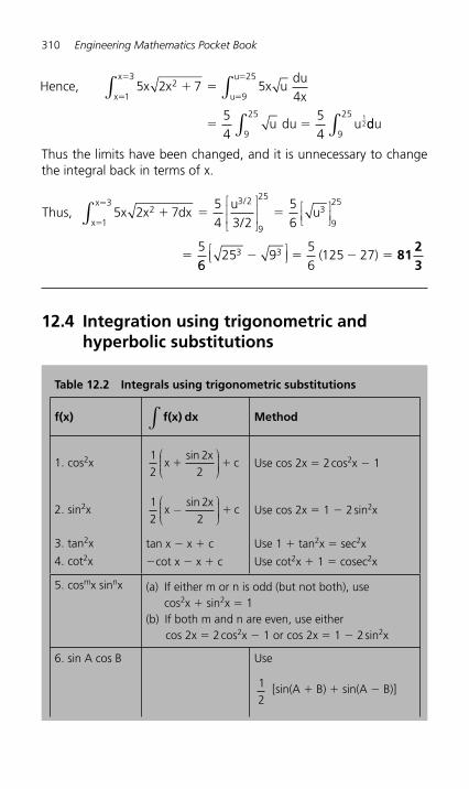
310 Engineering Mathematics Pocket Book
Hence, x x x udu4x
u du u
x
x
u
u5 2 7 5
54
54
21
3
9
25
9
25
9
25 12
� �
� �
�
�
�
�
∫ ∫
∫ ∫ ddu
Thus the limits have been changed, and it is unnecessary to change the integral back in terms of x.
Thus, x xu
/u
x
x /5 2 7
54 3 2
56
5
21
3 3 2
9
253
9
25� � �
�
�
�dx∫
⎡
⎣⎢⎢
⎤
⎦⎥⎥
⎡⎣⎢
⎤⎦⎥
6625 9
56
125 273 3� � � �⎡⎣⎢
⎤⎦⎥ ( ) 81
23
12.4 Integration using trigonometric and hyperbolic substitutions
Table 12.2 Integrals using trigonometric substitutions
f(x)
f(x) dx∫ Method
1. cos 2 x
12
22
xsin x
c� �⎛
⎝⎜⎜⎜
⎞
⎠⎟⎟⎟⎟
Use cos 2x � 2 cos 2 x � 1
2. sin 2 x
12
22
xsin x
c−⎛
⎝⎜⎜⎜
⎞
⎠⎟⎟⎟⎟ �
Use cos 2x � 1 � 2 sin 2 x
3. tan 2 x tan x � x � c Use 1 � tan 2 x � sec 2 x
4. cot 2 x � cot x � x � c Use cot 2 x � 1 � cosec 2 x
5. cos m x sin n x (a) If either m or n is odd (but not both), use cos2 x � sin 2 x � 1
(b) If both m and n are even, use either cos 2x � 2 cos 2 x � 1 or cos 2x � 1 � 2 sin 2 x
6. sin A cos B Use
12
[sin(A � B) � sin(A � B)]
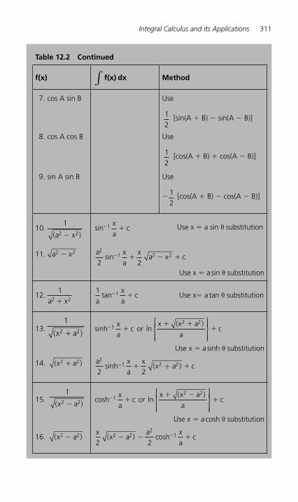
Integral Calculus and its Applications 311
Table 12.2 Continued
f(x)
f(x) dx∫ Method
7. cos A sin B Use
12
[sin(A � B) � sin(A � B)]
8. cos A cos B Use
12
[cos(A � B) � cos(A � B)]
9. sin A sin B Use
�
12
[cos(A � B) � cos(A � B)]
10.1
2 2( )a � x sin
xa
c1� � Use x � a sin θ substitution
11. a2 2� x
a xa
a2
2 2
2 2sin
xx c1� � � �
Use x � a sin θ substitution
12.1
2 2a x�
1 1
atan� �
xa
c Use x � a tan θ substitution
13.1
2 2( )x a�
sinh( )
� �� �
�12 2x
ac or ln
x x a
ac
⎧⎨⎪⎪⎪
⎩⎪⎪⎪
⎫⎬⎪⎪⎪
⎭⎪⎪⎪
Use x � a sinh θ substitution
14. ( )x a2 2�
a xa
xx a c
21 2 2
2 2sinh ( )− +� �
15. 1
2 2( )x a�
cosh( )
� �� �
�12 2x
ac or ln
x x a
ac
⎧⎨⎪⎪⎪
⎩⎪⎪⎪
⎫⎬⎪⎪⎪
⎭⎪⎪⎪
Use x � a cosh θ substitution
16. ( )x a2 2�
xx a c
2 22 2
21( )� � ��a
coshxa
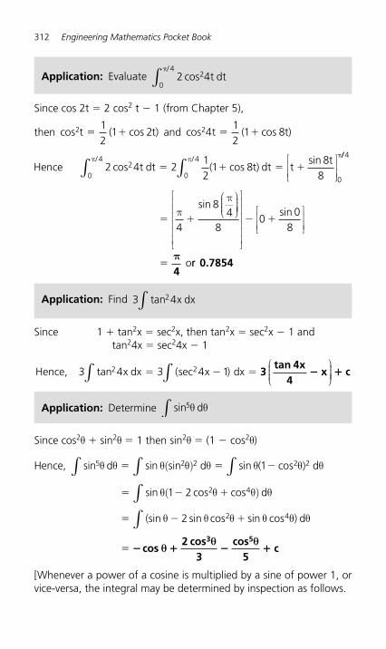
312 Engineering Mathematics Pocket Book
Since cos 2t � 2 cos 2 t � 1 (from Chapter 5),
then cos cos2 12
1 2t ( t)� � and cos cos2412
1 8t ( t)� �
Hence t dt ( cos t) dt t
t/ /2 4 2
12
1 88
82
0
4
0
4
0
cossinπ π π
∫ ∫⎡
⎣⎢⎢
⎤
⎦⎥⎥
� � � �// 4
� � � �
�
ππ
4
84
80
08
sinsin
⎛⎝⎜⎜⎜
⎞⎠⎟⎟⎟⎟
⎡
⎣
⎢⎢⎢⎢⎢⎢
⎤
⎦
⎥⎥⎥⎥⎥⎥
⎡
⎣⎢⎢
⎤
⎦⎥⎥
π4
orr 0.7854
Application: Evaluate 2 420
4cos t dt
/π
∫
Application: Find 3 42tan∫ x dx
Since 1 � tan 2 x � sec 2 x, then tan 2 x � sec 2 x � 1 and tan 2 4x � sec 24x � 1
Hence, tan x dx sec x dx3 4 3 4 12 2� � �( )∫∫
⎛⎝⎜⎜⎜
⎞⎠⎟⎟⎟⎟3
tan 4x4
x c� �
Application: Determine sin d5∫ θ θ
Since cos 2 θ � sin 2 θ � 1 then sin 2 θ � (1 � cos 2 θ )
Hence, sin d sin sin d cos d5 2 2 2 21θ θ θ( θ) θ θ θ θ� � �∫∫ ∫ sin ( )
� � �
� � �
�
sin cos cos
(sin sin cos sin cos )
θ( θ θ) θ
θ θ θ θ θ θ
1 2
2
2 4
2 4
∫
∫
d
d
� cos2 cos
3cos
5c
3 5θ
θ θ� � �
[Whenever a power of a cosine is multiplied by a sine of power 1, or vice-versa, the integral may be determined by inspection as follows.
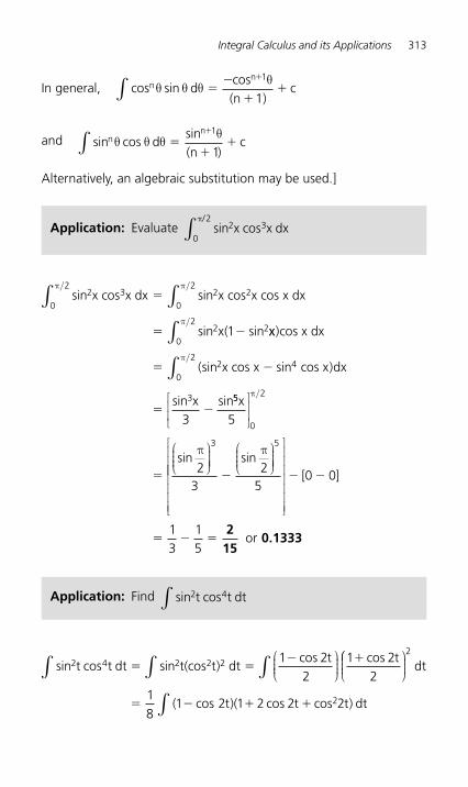
Integral Calculus and its Applications 313
In general, cos dcos(n 1)
cnn
∫ θ θ θθ
sin ��
��
�1
and sin cosn∫ θ θ θθ
dsin(n )
cn
��
��1
1
Alternatively, an algebraic substitution may be used.]
Application: Evaluate sin x cos x dx/
2 30
2π
∫
sin x cos x dx sin x cos x cos x dx
sin x sin
2 30
22
0
22
2 21
π/ π/
∫ ∫�
� �( xx cos x dx
sin x cos x sin cos x dx
sin x sin
)
( )
0
2
2 40
2
3
3
π/
π/
∫
∫� �
� �55
0
2
3 5
5
23
25
x
sin sin
⎡
⎣⎢⎢
⎤
⎦⎥⎥
⎛⎝⎜⎜⎜
⎞⎠⎟⎟⎟⎟
⎛⎝⎜⎜⎜
⎞⎠⎟⎟⎟⎟
⎡
⎣
⎢⎢
π/
π π
� �⎢⎢⎢⎢⎢⎢
⎤
⎦
⎥⎥⎥⎥⎥⎥⎥
� �
� � �
[ ]
or
0 0
13
15
215
0.1333
Application: Find sin t cos t dt2 4∫
sin cos sin (cos )cos cos2 4 2 2 2 1 22
1 22
t t dt t t dtt t
∫ ∫ ∫⎛⎝⎜⎜⎜
⎞⎠⎟⎟⎟� �
� �⎛⎛⎝⎜⎜⎜
⎞⎠⎟⎟⎟
∫
2
218
1 2 1 2 2 2
dt
t t dt� � � �( )( cos cos )cos t
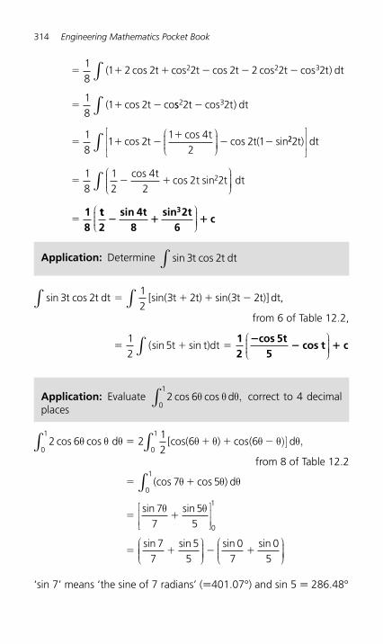
314 Engineering Mathematics Pocket Book
� � � � � �
� � �
18
1 2 2 2 2 2 2 2
18
1 2
2 2 3( cos cos cos cos cos )
( cos co
t t t t t dt
t
∫
ss cos )
coscos
cos sin
2 32 2
18
1 21 4
22 1
t t dt�
� � ��
� �
∫⎛⎝⎜⎜⎜
⎞⎠⎟⎟⎟⎟t
tt( 22
2
2
18
12
42
2
t)
t2t t dt
⎡
⎣⎢⎢
⎤
⎦⎥⎥
⎛⎝⎜⎜⎜
⎞⎠⎟⎟⎟⎟
∫
∫
dt
� � �
�
coscos sin
18
tt2
sin 4t8
sin 2t6
c3
� � �⎛
⎝⎜⎜⎜
⎞
⎠⎟⎟⎟⎟
Application: Determine sin cos3 2t t dt∫
sin t cos t dt [sin( t t) sin( t t)] dt,3 2
12
3 2 3 2� � � �∫∫
from 6 of Table 12.2 ,
� � �12
5( t t)dtsin sin12
cos 5t5
cos t c�
� �⎛⎝⎜⎜⎜
⎞⎠⎟⎟⎟⎟∫
Application: Evaluate 2 60
1cos cosθ θ θ,∫ d correct to 4 decimal
places
2 2
12
6 60
1
0
1cos cos cos6 d [cos( ) ( dθ θ θ θ θ θ θ)] θ,∫ ∫� � � �
from 8 of Table 12.2
� �
� �
� �
(cos cos )
sin sin
sin sin
7 5
77
55
77
55
0
1
0
1
θ θ θ
θ θ
∫⎡
⎣⎢⎢
⎤
⎦⎥⎥
⎛⎝⎜
d
⎜⎜⎜⎞⎠⎟⎟⎟⎟
⎛⎝⎜⎜⎜
⎞⎠⎟⎟⎟⎟� �
sin sin07
05
‘ sin 7 ’ means ‘ the sine of 7 radians ’ ( �401.07 ° ) and sin 5 � 286.48 °
Integral Calculus and its Applications 315
Hence, 2 6 0 09386 0 19178 00
1cos cos ( . . ) ( )θ θ θd � �� �∫
� � 0.0979, correct to 4 decimal places
Application: Evaluate 16 20
4� x dx∫
From 11 of Table 12.2 ,
16162 4 2
1620
41 2
0
4
� � � ��x dx sinx x
( x )∫⎡
⎣⎢⎢
⎤
⎦⎥⎥
� � � �
� � �
� �
�
8 1 2 0 8 0 0
8 1 82
1 1
1
sin sin
sin
⎡⎣⎢
⎤⎦⎥
⎛⎝⎜⎜⎜
⎞⎠⎟⎟⎟⎟
[ ]
orπ
4 1π 22.57
Application: Evaluate 1
4 20
2
( x )dx
�∫
From 12 of Table 12.2 , 1
412 220
21
0
2
( x )dx tan
x�
� �∫⎡
⎣⎢⎢
⎤
⎦⎥⎥
since a � 2
� �
� �
�
� �12
1 0
12 4
0
1 1( )
or
tan tan
π⎛⎝⎜⎜⎜
⎞⎠⎟⎟⎟⎟
π8
0.3927
Application: Evaluate 1
420
2
(x )dx,
�∫ correct to 4 decimal
places
1
421
0
2
0
2
(x )dx sinh
x2�
� �⎡
⎣⎢⎢
⎤
⎦⎥⎥∫
or lnx (x )� �2
0
24
2
⎧⎨⎪⎪⎪
⎩⎪⎪⎪
⎫⎬⎪⎪⎪
⎭⎪⎪⎪
⎡
⎣
⎢⎢⎢
⎤
⎦
⎥⎥⎥
from 13 of Table 12.2 , where a � 2
316 Engineering Mathematics Pocket Book
Using the logarithmic form,
1
4
2 82
0 4220
2
(x )dx ln ln
��
��
�∫
⎛
⎝⎜⎜⎜⎜
⎞
⎠⎟⎟⎟⎟⎟
⎛
⎝⎜⎜⎜⎜
⎞
⎠⎟⎟⎟⎟⎟
⎡
⎣
⎢⎢⎢
⎤
⎦⎦
⎥⎥⎥
� �
�
ln ln
, correct to 4 decimal places
2 4142 1.
0.8814
Application: Determine 2 3
92
x
(x )dx
�
�∫
2 3
9
2
9
3
92 2 2
x
(x )dx
x
(x )dx
(x )dx
�
��
��
�∫ ∫∫
The first integral is determined using the algebraic substitution
u � (x 2 � 9), and the second integral is of the form 1
2 2(x a )dx
�∫
(see 15 of Table 12.2 )
Hence,
2
9
3
92 2
x
(x )dx
(x )dx
��
��∫ ∫ 2 (x 9) 3 cosh
x3
c2 1� � ��
Application: Evaluate (x ) dx22
34�∫
(x ) dx
x2
(x ) coshx2
22
32 1
2
3
4 442
� � � � �∫⎡
⎣⎢⎢
⎤
⎦⎥⎥
from 16 of Table 12.2 , when a � 2,
� � � �
�
� �32
5 232
0 2 11 1cosh cosh
, by calcul
⎛⎝⎜⎜⎜
⎞⎠⎟⎟⎟⎟ ( )
1.429 aator
or since coshxa
lnx (x a )
a� �
� �12 2⎧
⎨⎪⎪⎪
⎩⎪⎪⎪
⎫⎬⎪⎪⎪
⎭⎪⎪⎪
then cosh ln( )� �
� �12 23
23 3 2
2
⎧⎨⎪⎪⎪
⎩⎪⎪⎪
⎫⎬⎪⎪⎪
⎭⎪⎪⎪
� ln 2.6180 � 0.9624
Integral Calculus and its Applications 317
Similarly, cosh � 1 1 � 0
Hence, (x ) dx ( ) [0]22
34
32
5 2 0 9624� � � �∫⎡
⎣⎢⎢
⎤
⎦⎥⎥
.
� 1.429 , correct to 4 significant figures
12.5 Integration using partial fractions
1. Linear factors
Application: Determine 11 3
2 32
�
� �
xx x
dx∫
As shown on page 42: 11 32 3
21
532
�
� � ��
�
xx x (x ) (x )
�
Hence 11 3
2 32
15
32
�
� ��
��
�
�
xx x
dx(x ) (x )
dx∫ ∫⎧⎨⎪⎪⎩⎪⎪
⎫⎬⎪⎪⎭⎪⎪
2 ln(x 1) 5� � lln(x 3) c� � (by algebraic substitutions (see section 12.3))
or ln(x 1)(x 3)
c2
5
�
��
⎧⎨⎪⎪⎩⎪⎪
⎫⎬⎪⎪⎭⎪⎪
by the laws of logarithms
Application: Evaluate x x x
x xdx,
3 2
22
3 2 4 42
� � �
� �∫ correct to 4 significant figures
By dividing out and resolving into partial fractions, it was shown on page 43:
x x xx x
x(x ) (x )
3 2
2
2 4 42
34
23
1� � �
� �� �
��
��
Hence,
x x xx x
dx x(x ) (x )
dx3 2
2 2
3
2
2 4 42
34
23
1� � �
� �� �
��
��
⎧⎨⎪⎪⎩⎪⎪
⎫⎬⎪⎪⎭⎪⎪
∫33
∫
318 Engineering Mathematics Pocket Book
� � � � � �
� � � �
xx ln(x ) ln(x )
2
2
3
23 4 2 3 1
92
9 4 5 3 2
⎡
⎣⎢⎢
⎤
⎦⎥⎥
⎛⎝⎜⎜⎜
⎞ln ln
⎠⎠⎟⎟⎟⎟ � � � �( )2 6 4 4 3 1ln ln
� � 1.687 , correct to 4 significant figures
2. Repeated linear factors
Application: Find 5 2 193 1
2
2
x x(x )(x )
dx� �
� �∫
It was shown on page 44:
5 2 193 1
23
21
41
2
2 2
x x(x )(x ) (x ) (x ) (x )
� �
� � ��
��
��
Hence, 5 2 19
3 12
33
14
1
2
2 2
x x(x )(x )
dx(x ) (x ) (x )
� �
� � ��
��
�∫⎧⎨⎪⎪⎩⎪⎪
⎫⎬⎪⎪⎭
�⎪⎪⎪
∫ dx
� 2 ln(x 3) 3 ln(x 1)4
(x 1)c� � � �
��
or ln{(x 3) (x 1) }4
(x 1)c2 3� � �
��
3. Quadratic factors
Application: Find 3 6 4 2
3
2 3
2
� � �
�
x x xx (x )
dx2∫
It was shown on page 45: 3 6 4 23
2 1 3 43
2 2
2 2 2 2
� � �
�� �
�
�
x x xx (x ) x x
x(x )
�
Integral Calculus and its Applications 319
Thus,
3 6 4 23
2 1 3 43
2 3
2 2 2 2
� � �
�� �
�
�
x x xx (x )
dxx x
x(x )
dx∫ ∫⎛
⎝⎜⎜⎜⎜
⎞
⎠⎟⎟⎟⎟�
�� � ��
��
2 1 33
432 2 2x x (x )
x(x )
dx⎧⎨⎪⎪⎩⎪⎪
⎫⎬⎪⎪⎭⎪⎪
∫
33
31
3
3
3 322
21
(x )dx
xdx tan
x,
��
�� �
( )∫∫
from 12, Table 12.2 , page 311.
432
xx
dx�∫ is determined using the algebraic substitution
u � (x 2 � 3)
Hence, x x (x )
x(x )
dx2 1 3
34
32 2 2� �
��
�
�
⎧⎨⎪⎪⎩⎪⎪
⎫⎬⎪⎪⎭⎪⎪
∫
2 ln x1x
� �� � � ��33
tanx3
2 ln(x 3) c1 2
or lnx
x 31x
3 tanx3
c2
21
�� � ��
⎛⎝⎜⎜⎜
⎞⎠⎟⎟⎟⎟
12.6 The t tan2
�θ
substitution
To determine 1
a b cd
cos sinθ θθ,
� �∫ where a, b and c are
constants, if t tan�θ2
then:
sin2t
(1 t )2θ �
�(1)
cos1 t1 t
2
2θ �
�
�(2)
d2dt
1 t2θ �
�(3)
320 Engineering Mathematics Pocket Book
If t tan�θ2
then sin θ ��
21 2
tt
and ddt
tθ �
�
21 2
from equations
(1) and (3).
Thus,d
tt
dtt t
dt ln t cθθsin
�
��
� � �12
1
21
1
2
2
⎛⎝⎜⎜⎜
⎞⎠⎟⎟⎟⎟ ∫∫∫
Hence, d
sinln tan
2c
θθ
θ� �
⎛⎝⎜⎜⎜
⎞⎠⎟⎟⎟⎟∫
Application: Determine dθ
θsin∫
Application: Determine dx
xcos∫
If tanx2
then cos xtt
��
�
11
2
2 and dxdt
t�
�
21 2 from equations (2)
and (3).
Thusdx
x tt
dtt t
dtcos∫ ∫ ∫
⎛⎝⎜⎜⎜
⎞⎠⎟⎟⎟⎟�
�
�
��
�
111
21
212
2
2 2
21 2� t
may be resolved into partial fractions (see section 2.10)
Let 21
21 1 1 1
1 11 12�
�� �
��
��
�� � �
� �t ( t)( t)A
( t)B
( t)A( t) B( t)
( t)( t)
Hence 2 � A(1 � t) � B(1 � t)
When t � 1, 2 � 2A, from which, A � 1
When t � � 1, 2 � 2B, from which, B � 1
Hence, t t t
dt ln( t) ln( t) c2
11
11
11 1
2��
��
�� � � � � �
�
⎛⎝⎜⎜⎜
⎞⎠⎟⎟⎟⎟∫∫
lln( t)( t)
c11
�
��
⎧⎨⎪⎪⎩⎪⎪
⎫⎬⎪⎪⎭⎪⎪
Integral Calculus and its Applications 321
Thus,dx
cos xln
1 tanx2
1 tanx2
c∫⎧
⎨
⎪⎪⎪⎪⎪
⎩⎪⎪⎪⎪⎪
⎫
⎬
⎪⎪⎪⎪⎪
⎭⎪⎪⎪⎪⎪
��
��
Note that since tan π4
1� , the above result may be written as:
dxx
lntan tan
x
tan tanxcos
��
�
π
π4 2
4 2
⎧
⎨
⎪⎪⎪⎪⎪
⎩⎪⎪⎪⎪⎪
⎫
⎬
⎪⎪⎪⎪⎪
⎭⎪⎪⎪⎪⎪
∫ �� �c ln tan4
x2
cπ
� �⎛⎝⎜⎜⎜
⎞⎠⎟⎟⎟⎟
⎧⎨⎪⎪⎩⎪⎪
⎫⎬⎪⎪⎭⎪⎪
from compound angles, chapter 5.
Application: Determine dθ
θ5 4� cos∫
If t tan�θ2
then cos θ ��
�
11
2
2
tt
and ddtt
θ ��
21 2
from equations (2) and (3).
Thus,cos
d
tt
dtt
θθ5 4
1
5 411
212
2
2��
��
�
�∫ ⎛
⎝⎜⎜⎜⎜
⎞
⎠⎟⎟⎟⎟
⎛⎝⎜⎜⎜
⎞⎠⎟⎟⎟⎟∫∫
∫⎛
⎝⎜⎜⎜⎜
⎞
⎠⎟⎟⎟⎟�
� � �
�
�
15 1 4 1
1
212 2
2
2( t ) ( tt
dt( t) )
��
��
� ��29
23
213 32 2 2
1dtt
dtt
tant
c⎛⎝⎜⎜⎜
⎞⎠⎟⎟⎟⎟∫∫
Hence, d4
θθ
θ5 cos
23
tan13
tan2
c1
�� ��
⎛⎝⎜⎜⎜
⎞⎠⎟⎟⎟⎟∫
Application: Determine dxx xsin cos�∫
If t tanx
�2
then sin xtt
cos xtt
��
��
�
21
112
2
2, and dx
dtt
��
21 2
from equations (1), (2) and (3).
322 Engineering Mathematics Pocket Book
Thus,dx
x x
dtt
tt
tt
sin cos�� �
��
�
�
∫ ⎛⎝⎜⎜⎜
⎞⎠⎟⎟⎟⎟
⎛
⎝⎜⎜⎜⎜
⎞
⎠⎟⎟⎟⎟
21
21
11
2
2
2
2
∫∫ ∫
∫ ∫
� �� �
�
�� �
��
� �
21
2 11
21 2
22 1
2
2
2
2 2
dtt
t tt
dtt t
dtt t
��
� ��
� �
�� �
� �
21 2
2
2 1
21
2 2
2 1
2 1
2 22
dt(t )
dt
(t )
ln(t )
(t
∫ ∫( )
⎧⎨⎪⎪
⎩ )⎪⎪⎪
⎫⎬⎪⎪
⎭⎪⎪
⎡
⎣
⎢⎢⎢
⎤
⎦
⎥⎥⎥� c
by using partial fractions 1 1
22 2a xdx
aln
a xa x�
��
�
⎛⎝⎜⎜⎜
⎞⎠⎟⎟⎟⎟∫
i.e. dx
x xsin cos��
12
ln2 1 tan
x2
2 1 tanx2
� �
� �
⎧
⎨
⎪⎪⎪⎪⎪
⎩⎪⎪⎪⎪⎪
⎫
⎬
⎪⎪⎪⎪⎪
⎭⎪⎪⎪⎪⎪⎪
∫ � c
Application: Determine dxx x7 3 6� �sin cos∫
From equations (1) to (3),
dxx x
dtt
tt
tt
7 3 6
21
7 32
16
11
2
2
2
2
� �� �
��
��
�
sin cos∫ ⎛⎝⎜⎜⎜
⎞⎠⎟⎟⎟
⎛⎝⎜⎜⎜
⎞⎞⎠⎟⎟⎟⎟
∫
∫� �� � � �
�
�� � � �
21
7 1 3 2 6 11
27 7 6 6 6
2
2 2
2
2
dtt
t t tt
dtt t
( ) ( ) ( )
ttdt
t tdt
t
2
2 2 2
26 13
23 2
∫
∫ ∫�� �
�� �( )
Integral Calculus and its Applications 323
�
���2
12
32
1tant
c⎛⎝⎜⎜⎜
⎞⎠⎟⎟⎟⎟
⎡
⎣⎢⎢
⎤
⎦⎥⎥
from 12 of Table 12.2 , page 311.
Hence,dxx x7 3 6� �
�sin cos
tantan
x2
3
2c1�
��
⎛
⎝
⎜⎜⎜⎜⎜⎜⎜⎜⎜
⎞
⎠
⎟⎟⎟⎟⎟⎟⎟⎟⎟⎟∫
12.7 Integration by parts
If u and v are both functions of x, then:
udvdx
dx uv vdudx
dx� � ∫∫∫
or u dv uv v du� � ∫∫
This is known as the integration by parts formula .
Application: Determine x x dxcos∫
From the integration by parts formula, udv uv vdu� � ∫∫ Let u � x, from which
dudx
� 1, i.e. du � dx
and let dv � cos x dx, from which v x dx x� �cos sin∫
Expressions for u, du, v and dv are now substituted into the ‘ by parts ’ formula as shown below.
∫ u dv � u v � ∫ v du
∫ x cos x dx � (x) (sin x) � ∫ (sin x) (dx)
i.e. x x dx x x ( x) ccos sin cos� � � � � x sin x cos x c� �∫
324 Engineering Mathematics Pocket Book
[This result may be checked by differentiating the right-hand side, i.e.
ddx
(x x x c) [(x)( x) (sin x)( )] sin xsin cos cos� � � � � �1 0
using the product rule � x cos x, which is the function being integrated]
Application: Find 3 2t e dtt∫
Let u � 3t, from which, dudt
� 3, i.e. du � 3dt
and let dv � e 2t dt, from which, v e dt et t� �2 212∫
Substituting into udv uv vdu� � ∫∫ gives:
3 312
12
332
2 2 2 2t e dt e e t et t t� � �( ) ( )t dt⎛⎝⎜⎜⎜
⎞⎠⎟⎟⎟⎟
⎛⎝⎜⎜⎜
⎞⎠⎟⎟⎟⎟∫∫ tt t
tt
e dt
t ee
c
�
� � �
32
32
32 2
2
22
∫
⎛
⎝⎜⎜⎜⎜
⎞
⎠⎟⎟⎟⎟
Hence, 3t e dt32
e t12
c2t 2t� � �⎛⎝⎜⎜⎜
⎞⎠⎟⎟⎟⎟∫ , which may be checked by
differentiating
Application: Evaluate 20
2θ θ θ
πsin d
/
∫
Let u � 2 θ , from which, dudθ
� 2, i.e. du � 2d θ
and let dv � sin θ d θ , from which, v d� � �sin cosθ θ θ∫
Substituting into u dv uv v du� � ∫∫ gives:
2 2 2
2 2 2
θ θ θ θ θ θ θ
θ θ θ θ θ
sin ( )( cos ) ( cos )( )
cos cos co
d d
d
� � � �
� � � � �
∫∫∫ ss sinθ θ� �2 c
Integral Calculus and its Applications 325
Hence, 2 2 20
2
0
2θ θ θ θ θ θπ π
sin cos sind/ /
∫ [ ]� � �
� � � � �22 2
22
0 2π π π⎛
⎝⎜⎜⎜
⎞⎠⎟⎟⎟⎟
⎡
⎣⎢⎢
⎤
⎦⎥⎥cos sin sin[ 0]
� ( � 0 � 2) � (0 � 0) � 2
since cosπ2
0� and sinπ2
1�
Application: Determine x x dx2 sin∫
Let u � x 2 , from which, dudx
x,� 2 i.e. du � 2x dx,
and let dv � sin x dx, from which, v x dx x� � �sin cos∫
Substituting into u dv uv v du� � ∫∫ gives:
x x dx x
x x x x dx
2 2
2
2
2
sin ( )( cos ) ( cos )( )
cos cos
∫ ∫
∫⎡⎣⎢⎤
� � � �
� � �
x x x dx
⎦⎦⎥
The integral, x x dx,cos∫ is not a ‘standard integral ’ and it can only
be determined by using the integration by parts formula again.
From the first application, page 323, x x dx x x x xcos sin cos� �∫
Hence, x x dx x x {x x x} c2 2 2sin cos sin cos� � � � �∫
� � � � �
�
x2 2 2cos sin cosx x x x c
(2 x ) cos x 2x sin x c2� � � In general, if the algebraic term of a product is of power n, then the integration by parts formula is applied n times.
Application: Find x x dxln∫
The logarithmic function is chosen as the ‘ u part ’
Thus, when u � ln x, then dudx
�1x
, i.e. dudxx
�
326 Engineering Mathematics Pocket Book
Letting dv � x dx gives v x dxx
� �2
2∫
Substituting into u dv uv v du� � ∫∫ gives:
x x dxx x dx
x
xx
ln (ln )
ln
∫ ∫⎛
⎝⎜⎜⎜⎜
⎞
⎠⎟⎟⎟⎟
⎛
⎝⎜⎜⎜⎜
⎞
⎠⎟⎟⎟⎟� �
� �
x2 2
2
2 2
212
xx dxx
xx
c� � �2 2
212 2
ln⎛
⎝⎜⎜⎜⎜
⎞
⎠⎟⎟⎟⎟∫
Hence, x x dxln �x2
ln x12
c2
� �⎛⎝⎜⎜⎜
⎞⎠⎟⎟⎟∫ or
x4
(2 ln x 1) c2
� �
12.8 Reduction formulae
x e dx I x e n In xn
n xn� � � �1∫ (4)
x x dx I x x nx x n n Inn
n nncos sin cos ( )� � � � ���
121∫ (5)
x x dx I n n(n )Inn
nn
01
21π
π∫ cos � � � � ��� (6)
x x dx I x x nx x n(n )Inn
n nnsin cos sin� � � � � ���
121∫ (7)
sin sin cosnn
nndx I
nx x
nn
Ix � � � ���
�
1 112∫ (8)
cos x dx In
cos sin xn
nIn
nn
n� � ���
�
1 112∫ (9)
sin x dx cos x dx In
nIn
/n
n n0
2
0
2
21π π/
∫ ∫� � ��
� (10)
tan x dx Itann
Inn
n
n� ��
��
�
1
21x
∫ (11)
(ln x) dx I x(ln x) n Inn
nn� � � �1∫ (12)
Integral Calculus and its Applications 327
Integrals of the form x e dxn x∫
When using integration by parts, an integral such as x e dxx2∫
requires integration by parts twice. Similarly, x e dxx3∫
requires integration by parts three times. Thus, integrals such
as x e dx, x cos x dxx5 6∫∫ and x sin x dx8 2∫ for example,
would take a long time to determine using integration by parts.
Reduction formulae provide a quicker method for determining
such integrals.
Application: Determine x e dx3 x∫ using a reduction formula
From equation (4), I n � x n e x � nI n � 1
Hence x e dx I x ex x33
323∫ � � � I
I
I2
21
11
0
2
1
� �
� �
x e I
x e I
x
x
and I x e dx e dx e0x x� � �0 x∫ ∫
Thus x e dx x e [ x e I ]x x x3 3 213 2∫ � � �
� � � �
� � � �
� � �
x e x e (xe I )]
x e [x e (xe e )]
x e x e
x x x
x x x x
x x
3 20
3 2
3 2
3 2
3 2
3
[
66
3 6 63 2
(xe e )
x e x e xe e
x x
x x x x
�
� � � �
i.e. x e dx e ( x 3x 6x 6) c3 x x 3 2∫ � � � � �
Integrals of the form x cos x dxn∫
Application: Determine x x dx2cos∫ using a reduction formula
328 Engineering Mathematics Pocket Book
Using the reduction formula of equation (5):
x x dx2 cos∫ � I 2 � x 2 sin x � 2x 1 cos x � 2(1)I0
and I0 0� � �x x dx cos x dx xcos sin∫ ∫
Hence x cos x dx sin x 2xcos x 2sin x c2∫ � x2 � � �
Application: Evaluate 4 31
2t t dtcos∫ , correct to 4 significant
figures
From equation (5),
t t dt3cos∫ � I 3 � t 3 sin t � 3t 2 cos t � 3(2)I 1
and I 1 � t 1 sin t � 1 t 0 cos t � 1(0)I n � 2
� t sin t � cos t
Hence t t dt3cos∫ � t3 sin t � 3t2 cos t � 3(2) [t sin t � cos t]
� t 3 sin t � 3t 2 cos t � 6t sin t � 6 cos t
Thus, 4 4 3 6 631
23 2
1
2t dt t t t t t t tcos ( sin cos sin cos )t∫ ⎡
⎣⎢⎤⎦⎥� � � �
� � � �
� � �
[ ( sin cos sin cos )]
[ (sin cos s
4 8 2 12 2 12 2 6 2
4 1 3 1 6 iin cos )]
. . )
1 6 1
24 53628 23 31305
�
� � � �
�
( ) (
�1.223
Integrals of the form x sin x dxn∫
Application: Determine x x dx3 sin∫ using a reduction formula
Using equation (7),
x x dx3 sin∫ � I 3 � � x 3 cos x � 3x 2 sin x � 3(2)I 1
and I 1 � � x 1 cos x � 1x 0 sin x � � x cos x � sin x
Integral Calculus and its Applications 329
Hence,
x x dx3 sin∫ � � x 3 cos x � 3x 2 sin x � 6[ �x cos x � sin x]
� � x3 cos x � 3x2 sin x � 6x cos x � 6 sin x � c
Integrals of the form sin x dxn∫
Application: Determine sin dx4x∫ using a reduction formula
Using equation (8), sin x dx I sin x x I4 3� � � �4 214
34∫ cos
I 2 � � 12
sin 1 x cos x � 12
I 0 and I 0 � sin x dx dx x0∫ ∫� �1
Hence
sin x dx I sin x x (x)4 3∫⎡
⎣⎢⎢
⎤
⎦⎥⎥
� � � � � �414
34
12
12
cos sin cosx x
� � � � �14
sin x cos x38
sin x cos x38
x c3
Integrals of the form cos x dxn∫
Application: Determine cos4x dx∫ using a reduction formula
Using equation (9), cos x dx I cos x4 3� � �4 214
34
sin x I∫
and I x x2 012
12
� �cos sin I and I cos dx x0
0 1� � �x dx ∫∫
Hence, cos x dx cos x4 3� � �14
34
12
12
x x x xsin cos sin⎛⎝⎜⎜⎜
⎞⎠⎟⎟⎟⎟∫
�14
cos x sin x38
cos x sin x38
x c3 � � �
330 Engineering Mathematics Pocket Book
From equation (10), cos dx In
nIn
n
/
nx � ��
�0
2
21π
∫ (This is usually
known as Wallis’s formula )
Thus, cos x dx I5/
0
2
345
π
∫ �
I3 1
23
� I and I x dx x ( )/ /
11
0
2
02 1 0 1� � � � �cos sin
π π∫ [ ]
Hence cos50
2
3 145
45
23
45
23
1π/
x dx I ( )∫⎡
⎣⎢⎢
⎤
⎦⎥⎥
⎡
⎣⎢⎢
⎤
⎦⎥⎥
� � � �I8
15
Further reduction formulae
Application: Evaluate cos50
2x dx
/π
∫
Application: Determine tan x dx7∫
From equation (11), Inn
ntan x
nI�
��
�
�
1
21
When n � 7, I tan x dxtan x
I76
7 56� � �∫
I
tan xI
4
5 34� � and I
tan xI
2
3 12� �
I dx ln( x)1 � �tan secx∫
using tansincos
xxx
� and letting u � cos x
Thus tan x dxtan tan x tan x
(ln(sec x))76 4 2
� � � �x
6 4 2
⎛⎝⎜⎜⎜
⎞⎠⎟⎟⎟⎟
⎡
⎣⎢⎢
⎤
⎦⎥⎥⎥∫
Hence,
tan x dx16
tan x14
tan x12
tan x ln(sec x) c7 6 4 2� � � � �∫
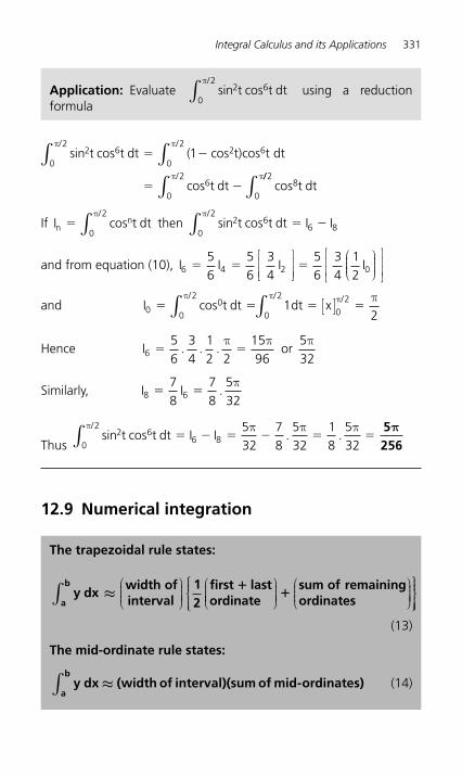
Integral Calculus and its Applications 331
sin cos cos cos
cos cos
2 60
22 6
0
2
6 80
1t t dt
t
π π
π
/ /( t) t dt
dt t dt
∫ ∫� �
� �/// 2
0
2
∫∫π
If I t dtn
/� cosn
0
2π
∫ then sin cos2 66 8
0
2t t dt I I
/� �
π
∫
and from equation (10), I I I I6 4 2 056
56
34
56
34
12
� � �⎡
⎣⎢⎢
⎤
⎦⎥⎥
⎛⎝⎜⎜⎜
⎞⎠⎟⎟⎟
⎡
⎣⎢⎢
⎤
⎦⎥⎥
and I t dt dt x/ / /
00
0
2
0
2
021
2� � � �cos
π π π π∫ ∫ [ ]
Hence I . . .656
34
12 2
1596
� �π π
or 532π
Similarly, I I .8 678
78
532
� �π
Thus sin cos2 6
60
2
8532
78
532
18
532
t t dt I I . ./
� � � � � �π π π π
∫5256
π
12.9 Numerical integration
Application: Evaluate sin cos2 6/
t t dt0
2π
∫ using a reduction formula
The trapezoidal rule states:
y dxwidth ofinterval
12
first lastordinatea
b
∫⎛⎝⎜⎜⎜
⎞⎠⎟⎟⎟⎟
⎛⎝⎜⎜≈ �⎜⎜
⎞⎠⎟⎟⎟⎟
⎛⎝⎜⎜⎜
⎞⎠⎟⎟⎟⎟
⎧⎨⎪⎪⎩⎪⎪
⎫⎬⎪⎪⎭⎪
�sum of remainingordinates ⎪⎪
(13)
The mid-ordinate rule states:
y dxa
b≈∫ (width of interval)(sum of mid-ordinates) (14)
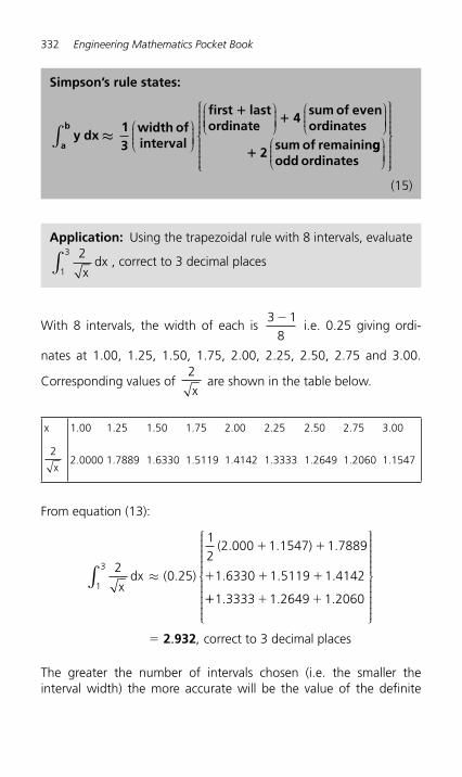
332 Engineering Mathematics Pocket Book
With 8 intervals, the width of each is 3 1
8�
i.e. 0.25 giving ordi-
nates at 1.00, 1.25, 1.50, 1.75, 2.00, 2.25, 2.50, 2.75 and 3.00.
Corresponding values of 2
x are shown in the table below.
x 1.00 1.25 1.50 1.75 2.00 2.25 2.50 2.75 3.00
2
x 2.0000 1.7889 1.6330 1.5119 1.4142 1.3333 1.2649 1.2060 1.1547
From equation (13):
20 25
12
1 1547 1 7889
1 6330 1 5119 1 41421
3
xdx
(2.000
∫ ≈ ( . )
. ) .
. . .
� �
� � �
�� � �
�
1 3333 1 2649 1 2060. . .
⎧
⎨
⎪⎪⎪⎪⎪⎪⎪
⎩
⎪⎪⎪⎪⎪⎪⎪
⎫
⎬
⎪⎪⎪⎪⎪⎪⎪
⎭
⎪⎪⎪⎪⎪⎪⎪
2.. ,932 correct to 3 decimal places
The greater the number of intervals chosen (i.e. the smaller the interval width) the more accurate will be the value of the definite
Simpson’s rule states:
y dx13
width ofinterval
first lastordinate
a
b≈∫
⎛⎝⎜⎜⎜
⎞⎠⎟⎟⎟⎟
⎛⎝⎜⎜
�⎜⎜
⎞⎠⎟⎟⎟⎟
⎛⎝⎜⎜⎜
⎞⎠⎟⎟⎟⎟�
�
4sum of evenordinates
2sum of remaininggodd ordinates
⎛⎝⎜⎜⎜
⎞⎠⎟⎟⎟⎟
⎧
⎨
⎪⎪⎪⎪⎪
⎩
⎪⎪⎪⎪⎪
⎫
⎬
⎪⎪⎪⎪⎪
⎭
⎪⎪⎪⎪⎪
(15)
Application: Using the trapezoidal rule with 8 intervals, evaluate 2
1
3
xdx∫
, correct to 3 decimal places
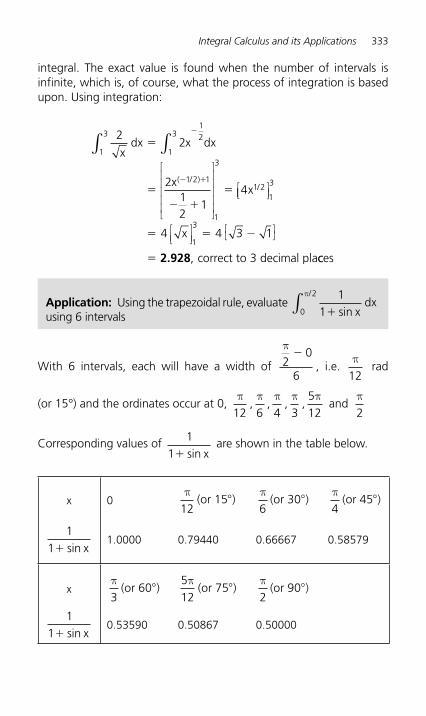
Integral Calculus and its Applications 333
integral. The exact value is found when the number of intervals is infinite, which is, of course, what the process of integration is based upon. Using integration:
22
212
14
1
3
1
312
1 2 1
1
3
1 2
xdx dx
xx
//
∫ ∫⎡
⎣
⎢⎢⎢⎢⎢
⎤
⎦
⎥⎥⎥⎥⎥
⎡⎣
�
�
� �
�
�
� �
x
( )
⎢⎢ ⎤⎦⎥
⎡⎣⎢
⎤⎦⎥
⎡⎣ ⎤⎦
1
3
1
34 4 3 1� � �
�
x
correct to 3 decimal pla2 928. , cces
Application: Using the trapezoidal rule, evaluate 1
10
2
� sin xdx
/π
∫ using 6 intervals
With 6 intervals, each will have a width of
π2
0
6
� , i.e.
π12
rad
(or 15°) and the ordinates occur at 0, π π π π π π
12 6 4 3 12 2, , , ,
5 and
Corresponding values of 11� sin x
are shown in the table below.
x 0
π12
(or 15 )�
π6
(or 30 )�
π4
(or 45 )�
11� sin x
1.0000 0.79440 0.66667 0.58579
x
π3
(or 60 )�
512
π(or 75 )�
π2
(or 90 )�
11� sin x
0.53590 0.50867 0.50000
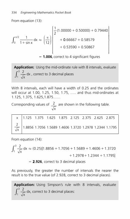
334 Engineering Mathematics Pocket Book
From equation (13):
11 12
12
1 00000 0 50000 0 79440
0
2
�
� �
�sin
( . . ) .
xdx
/π≈
π∫
⎛⎝⎜⎜⎜
⎞⎠⎟⎟⎟⎟ 00 66667 0 58579
0 53590 0 50867
. .
. .
�
� �
⎧
⎨
⎪⎪⎪⎪⎪⎪⎪⎪
⎩
⎪⎪⎪⎪⎪⎪⎪⎪
⎫
⎬
⎪⎪⎪⎪⎪⎪⎪⎪⎪
⎭
⎪⎪⎪⎪⎪⎪⎪⎪� 1.006 , correct to 4 significant figures
Application: Using the mid-ordinate rule with 8 intervals, evaluate 2
1
3
xdx∫
, correct to 3 decimal places
With 8 intervals, each will have a width of 0.25 and the ordinates will occur at 1.00, 1.25, 1.50, 1.75, ….. and thus mid-ordinates at 1.125, 1.375, 1.625,1.875 … …
Corresponding values of 2
x are shown in the following table.
x 1.125 1.375 1.625 1.875 2.125 2.375 2.625 2.875
2
x 1.8856 1.7056 1.5689 1.4606 1.3720 1.2978 1.2344 1.1795
From equation (14):
20 25 1 7056 1 5689 1 4606 1 3720
1
3
xdx 1.8856∫ ≈ ( . )[ . . . .� � � �
� � �
�
1 2978 1 2344 1 1795. . . ]
22.926, correct to 3 decimal places
As previously, the greater the number of intervals the nearer the result is to the true value (of 2.928, correct to 3 decimal places).
Application: Using Simpson’s rule with 8 intervals, evaluate 2
1
3
xdx∫
, correct to 3 decimal places:
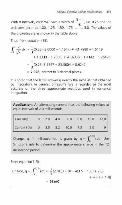
Integral Calculus and its Applications 335
With 8 intervals, each will have a width of 3 1
8�
, i.e. 0.25 and the
ordinates occur at 1.00, 1.25, 1.50, 1.75, … … , 3.0. The values of
the ordinates are as shown in the table above
Thus, from equation (15):
2 13
1 1547 4 1 7889 1 5119
1 33
1
3
xdx (0.25)[(2.0000∫ ≈ � � �
�
. ) ( . .
. 333 1 2060 2 1 6330 1 4142 1 2649
13
23 36
� � � �
� �
. ) ( . . . )
.
]
(0.25)[3.1547 004 8 6242�
�
. ]
2.928, correct to 3 decimal places
It is noted that the latter answer is exactly the same as that obtained by integration. In general, Simpson’s rule is regarded as the most accurate of the three approximate methods used in numerical integration.
Application: An alternating current i has the following values at equal intervals of 2.0 milliseconds.
Time (ms) 0 2.0 4.0 6.0 8.0 10.0 12.0
Current i (A) 0 3.5 8.2 10.0 7.3 2.0 0
Charge, q, in millicoulombs, is given by q i dt�0
12 0.
∫ . Use
Simpson’s rule to determine the approximate charge in the 12
millisecond period
From equation (15):
Charge, q i dt� � � � �
0
12 0 13
2 0 0 0 4 3 5 10 0 2 0.
( . )[( ) ( . . . )∫ ≈
� ��
2 8 2 7 3( . . )]62 mC
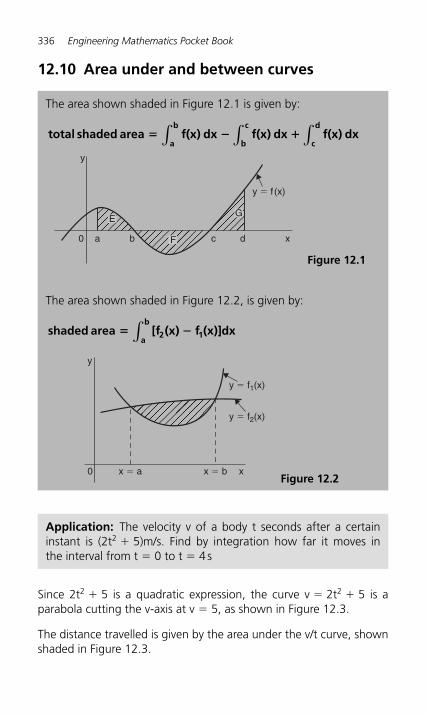
336 Engineering Mathematics Pocket Book
12.10 Area under and between curves
The area shown shaded in Figure 12.1 is given by:
total shaded area f(x) dx f(x) dx f(x) dxc
d
b
c
a
b� � � ∫∫∫
The area shown shaded in Figure 12.2 , is given by:
shaded area [f (x) f (x)]dx2 1a
b� �∫
E
0 F
G
y
a b c d
y � f (x)
x
Figure 12.1
y
x0 x � a
y � f2(x)
y � f1(x)
x � b Figure 12.2
Application: The velocity v of a body t seconds after a certain instant is (2t 2 � 5)m/s. Find by integration how far it moves in the interval from t � 0 to t � 4 s
Since 2t 2 � 5 is a quadratic expression, the curve v � 2t 2 � 5 is a parabola cutting the v-axis at v � 5, as shown in Figure 12.3 .
The distance travelled is given by the area under the v/t curve, shown shaded in Figure 12.3 .
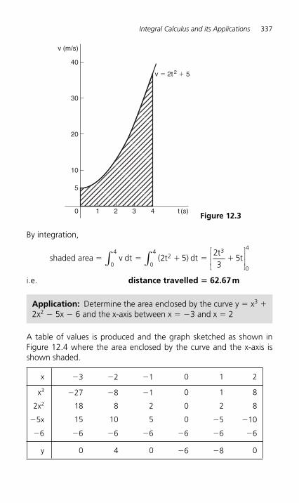
Integral Calculus and its Applications 337
By integration,
shaded area v dt t dtt
t� � � � �( )2 523
520
4
0
4 3
0
4
∫∫⎡
⎣⎢⎢
⎤
⎦⎥⎥
i.e. distance travelled � 62.67 m
40
30
20
10
5
1 2 3 40
v (m/s)
v � 2t 2 � 5
t (s) Figure 12.3
Application: Determine the area enclosed by the curve y � x 3 � 2x 2 � 5x � 6 and the x-axis between x � � 3 and x � 2
A table of values is produced and the graph sketched as shown in Figure 12.4 where the area enclosed by the curve and the x-axis is shown shaded.
x �3 �2 � 1 0 1 2
x 3 �27 �8 � 1 0 1 8
2x 2 18 8 2 0 2 8
� 5x 15 10 5 0 �5 � 10
�6 �6 �6 �6 �6 �6 � 6
y 0 4 0 �6 � 8 0
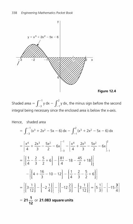
338 Engineering Mathematics Pocket Book
Shaded area � y dx y dx3
1
1
2
�
�
��∫ ∫ , the minus sign before the second
integral being necessary since the enclosed area is below the x-axis.
Hence, shaded area
� � � � � � � ��
�
�(x x ) dx (x x x ) dx3 2
3
13 2
1
22 5 6 2 5 6x∫ ∫
� � � � � � � �
�
�
�
�
x x xx
x x xx
4 3 2
3
1 4 3 2
1
2
423
52
64
23
52
6⎡
⎣⎢⎢
⎤
⎦⎥⎥
⎡
⎣⎢⎢
⎤
⎦⎥⎥
114
23
52
6814
18452
18� � � � � � �⎧⎨⎪⎪⎩⎪⎪
⎫⎬⎪⎪⎭⎪⎪
⎧⎨⎪⎪⎩⎪⎪
⎫⎬⎪⎪⎭⎪⎪
⎡
⎣⎢⎢
⎤
⎦⎦⎥⎥
⎧⎨⎪⎪⎩⎪⎪
⎫⎬⎪⎪⎭⎪⎪
⎧⎨⎪⎪⎩⎪⎪
⎫⎬⎪⎪⎭⎪⎪
⎡
⎣⎢� � � � � � � �4
163
10 1214
23
52
6⎢⎢⎤
⎦⎥⎥
⎧⎨⎪⎪⎩⎪⎪
⎫⎬⎪⎪⎭⎪⎪
⎧⎨⎪⎪⎩⎪⎪
⎫⎬⎪⎪⎭⎪⎪
⎡
⎣⎢⎢
⎤
⎦⎥⎥� � � � �3
112
214
1223
⎧⎧⎨⎪⎪⎩⎪⎪
⎫⎬⎪⎪⎭⎪⎪
⎧⎨⎪⎪⎩⎪⎪
⎫⎬⎪⎪⎭⎪⎪
⎡
⎣⎢⎢
⎤
⎦⎥⎥
⎡
⎣⎢⎢
⎤
⎦⎥⎥
� � � �31
125
13
15334
⎡
⎣⎢⎢
⎤
⎦⎥⎥
� 211
1221.083 square unitsor
y � x 3 � 2x 2 � 5x � 6
y
x�2 �1
6
20 1�3
Figure 12.4
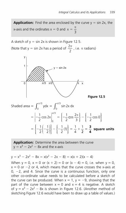
Integral Calculus and its Applications 339
A sketch of y � sin 2x is shown in Figure 12.5 .
(Note that y � sin 2x has a period of 22π
, i.e. π radians)
Application: Find the area enclosed by the curve y � sin 2x, the
x-axis and the ordinates x � 0 and x �π3
1
0 π/2 ππ/3
y � sin 2x
x
y
Figure 12.5
Shaded area ydx x dx
x
/ /
/
� �
� � � �
0
3
0
3
0
3
2
12
212
π
∫ ∫⎡
⎣⎢⎢
⎤
⎦⎥⎥
sin
cos
π
π
ccos23
12
0π⎧
⎨⎪⎪⎩⎪⎪
⎫⎬⎪⎪⎭⎪⎪
⎧⎨⎪⎪⎩⎪⎪
⎫⎬⎪⎪⎭⎪⎪
� � cos
� � � � � � �12
12
12
114
1⎛⎝⎜⎜⎜
⎞⎠⎟⎟⎟⎟
⎧⎨⎪⎪⎩⎪⎪
⎫⎬⎪⎪⎭⎪⎪
⎧⎨⎪⎪⎩⎪⎪
⎫⎬⎪⎪⎭⎪⎪
( )22
�34
square units
Application: Determine the area between the curve y � x 3 � 2x 2 � 8x and the x-axis
y � x 3 � 2x 2 � 8x � x(x 2 � 2x � 8) � x(x � 2)(x � 4)
When y � 0, x � 0 or (x � 2) � 0 or (x � 4) � 0, i.e. when y � 0,x � 0 or �2 or 4, which means that the curve crosses the x-axis at 0, �2, and 4. Since the curve is a continuous function, only one other co-ordinate value needs to be calculated before a sketch of the curve can be produced. When x � 1, y � �9, showing that the part of the curve between x � 0 and x � 4 is negative. A sketch of y � x3 � 2x2 � 8x is shown in Figure 12.6 . (Another method of sketching Figure 12.6 would have been to draw up a table of values.)
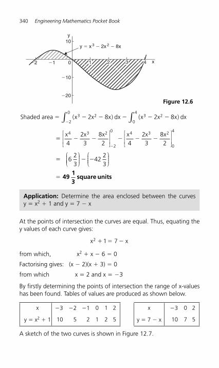
340 Engineering Mathematics Pocket Book
Shaded area x x x dx x x x dx� � � � � �
�( ) ( )3 2
2
03 2
0
42 8 2 8∫ ∫
� � � � � �
�
�
x x x x x x4 3 2
2
0 4 3 2
0
4
423
82 4
23
82
623
⎡
⎣⎢⎢
⎤
⎦⎥⎥
⎡
⎣⎢⎢
⎤
⎦⎥⎥
⎛⎝⎜⎜⎜⎜
⎞⎠⎟⎟⎟
⎛⎝⎜⎜⎜
⎞⎠⎟⎟⎟� �
�
4223
4913
square units
�1
�10
10
�20
0�2
y � x 3 � 2x 2 � 8x
x
y
1 2 3 4
Figure 12.6
Application: Determine the area enclosed between the curves y � x 2 � 1 and y � 7 � x
At the points of intersection the curves are equal. Thus, equating the y values of each curve gives:
x2 1 7� � � x
from which, x 2 � x � 6 � 0
Factorising gives: (x � 2)(x � 3) � 0
from which x � 2 and x � � 3
By firstly determining the points of intersection the range of x-values has been found. Tables of values are produced as shown below.
x �3 �2 � 1 0 1 2 x � 3 0 2
y � x 2 � 1 10 5 2 1 2 5 y � 7 � x 10 7 5
A sketch of the two curves is shown in Figure 12.7 .
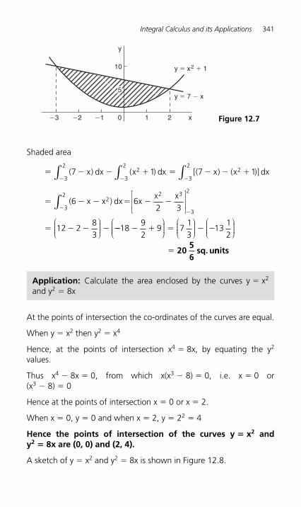
Integral Calculus and its Applications 341
Shaded area
� � � � � � � ��� �
( ) ( ) ) (7 1 7 123
2
3
22
3
2x dx x dx [( x x )] dx∫∫ ∫
� � � � � �
� � � �
��
(6 62 3
12 283
23
2 2 3
3
2
x x ) dx xx x
∫⎡
⎣⎢⎢
⎤
⎦⎥⎥
⎛⎝⎜⎜⎜
⎞⎠⎟⎟⎟ �� � � � � �
�
1892
9 713
1312
⎛⎝⎜⎜⎜
⎞⎠⎟⎟⎟
⎛⎝⎜⎜⎜
⎞⎠⎟⎟⎟
⎛⎝⎜⎜⎜
⎞⎠⎟⎟⎟
2056
sq. unnits
�3 �2 �1
10
1 20
y � x2 � 1
y � 7 � x
x
y
5
Figure 12.7
Application: Calculate the area enclosed by the curves y � x 2 and y 2 � 8x
At the points of intersection the co-ordinates of the curves are equal.
When y � x 2 then y 2 � x 4
Hence, at the points of intersection x 4 � 8x, by equating the y 2 values.
Thus x 4 � 8x � 0, from which x(x 3 � 8) � 0, i.e. x � 0 or (x3 � 8) � 0
Hence at the points of intersection x � 0 or x � 2.
When x � 0, y � 0 and when x � 2, y � 2 2 � 4
Hence the points of intersection of the curves y � x 2 and y2 � 8x are (0, 0) and (2, 4).
A sketch of y � x 2 and y 2 � 8x is shown in Figure 12.8 .
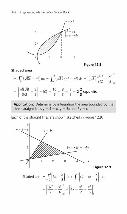
342 Engineering Mathematics Pocket Book
Shaded area
� � � � � �8 8 83 2 3
20
21 2 2
0
2 3 2 3
0
2
x x dx x x ) dxx
/x/
/( ) ( ) ( )⎡
⎣⎢⎢
⎤
⎦⎥⎥∫ ∫
� � � � � � �
8 83 2
83
0163
83
83/
⎧⎨⎪⎪
⎩⎪⎪
⎫⎬⎪⎪
⎭⎪⎪{ } 2
23
sq. units
4
y
y � 4 � x y � 3x
2
0 1 2 3 4 x
3y � x (or y � x3 )
Figure 12.9
2
0 1 2 x
4
y � x 2
y2 � 8x(or y � 8x)
Figure 12.8
Application: Determine by integration the area bounded by the three straight lines y � 4 � x, y � 3x and 3y � x
Each of the straight lines are shown sketched in Figure 12.9 .
Shaded area x dx ( x)x
dx
x
� � � � �
�
33
43
3
1
3
0
1 x⎛⎝⎜⎜⎜
⎞⎠⎟⎟⎟⎟
⎡
⎣⎢⎢
⎤
⎦⎥⎥∫∫
22 2
0
1 2 2
1
3
2 64
2 6� � � �
xx
x x⎡
⎣⎢⎢
⎤
⎦⎥⎥
⎡
⎣⎢⎢
⎤
⎦⎥⎥
Integral Calculus and its Applications 343
� � � � � � � � �32
16
0 1292
96
412
16
⎛⎝⎜⎜⎜
⎞⎠⎟⎟⎟⎟
⎡
⎣⎢⎢
⎤
⎦⎥⎥
⎛⎝⎜⎜⎜
⎞⎠⎟⎟⎟⎟
⎛( )
⎝⎝⎜⎜⎜
⎞⎠⎟⎟⎟⎟
⎡
⎣⎢⎢
⎤
⎦⎥⎥
⎛⎝⎜⎜⎜
⎞⎠⎟⎟⎟⎟
⎛⎝⎜⎜⎜
⎞⎠⎟⎟⎟⎟� � �
�
113
6 313
4 squarre units
12.11 Mean or average values
The mean or average value of the curve shown in Figure 12.10 , between x � a and x � b, is given by:
mean or average value, y1
b af(x)dx
a
b�
� ∫
y y � f (x)
x � a x � b x0
y
Figure 12.10
Application: Determine the mean value of y � 5x 2 between x � 1 and x � 4
Mean value, y y dx x dx
xx
��
�
� �
14 1
13
5
13
53
59
1
42
1
4
3
1
43
∫ ∫⎡
⎣⎢⎢
⎤
⎦⎥⎥
⎡⎣⎢⎢
⎤⎦⎥14 5
964 1� �
�
( )
35
344 Engineering Mathematics Pocket Book
Half a cycle means the limits are 0 to π radians.
Mean value, v
1v d( t) t d( t)�
��
πω
πω
π π
01
1000 0∫ ∫ sin ω
� � � � � �
� � � �
100 1000
1001 1
0πω
ππ
π
π[ cos t] [( cos ) ( cos )]
[( ) ( )] �� �200
π63.66 volts
[Note that for a sine wave, mean value � 2π
� maximum value
In this case, mean value � 2π
� 100 � 63.66 V]
Application: A sinusoidal voltage is given by v � 100 sin ωt volts. Determine the mean value of the voltage over half a cycle using integration
Application: The number of atoms, N, remaining in a mass of
material during radioactive decay after time t seconds is given by
N � N 0 e � λ t, where N 0 and λ are constants. Determine the mean
number of atoms in the mass of material for the time period
t � 0 and t �1λ
Mean number of atoms
�
�
� �� �11
0
110
1
00
1
00
1
λ λ
λλ
λλ
λλ
N dt N e dt N e dtt t/ / /
∫ ∫ ∫
��
� � � � � �
� �
�� �λ
λ
λ λλ λN
ee e N e e
N e
t
00
1
01 0
01 0
00
⎡
⎣⎢⎢
⎤
⎦⎥⎥
( )/
/[ ] [ ]N
�� � � �� �e N e 10
11⎡⎣⎢
⎤⎦⎥
⎡⎣⎢
⎤⎦⎥ 0.632 N0
Integral Calculus and its Applications 345
R.m.s. value y dx ( x ) dx��
�1
4 113
221
42 2
1
4
∫ ∫⎧⎨⎪⎪⎩⎪⎪
⎫⎬⎪⎪⎭⎪⎪
⎧⎨⎪⎪⎩⎪⎪⎪
⎫⎬⎪⎪⎭⎪⎪
⎧⎨⎪⎪⎩⎪⎪
⎫⎬⎪⎪⎭⎪⎪
∫�13
4 41
4x dx
� � �43 5
415
1024 15
1
4x⎡
⎣⎢⎢
⎤
⎦⎥⎥
⎧⎨⎪⎪⎪
⎩⎪⎪⎪
⎫⎬⎪⎪⎪
⎭⎪⎪⎪
⎧⎨⎪⎪⎩⎪⎪
⎫⎬⎪⎪⎭
( )⎪⎪⎪
� �272 8. 16.5
With reference to Figure 12.10 , the r.m.s. value of y � f(x) over the range x � a to x � b is given by:
r.m.s. value1
b ay dx2
a
b�
� ∫⎧⎨⎪⎪⎩⎪⎪
⎫⎬⎪⎪⎭⎪⎪
The r.m.s. value of an alternating current is defined as ‘that cur-rent which will give the same heating effect as the equivalent direct current ’ .
12.12 Root mean square values
Application: Determine the r.m.s. value of y � 2x 2 between x � 1 and x � 4
Application: A sinusoidal voltage has a maximum value of 100 V. Calculate its r.m.s. value
A sinusoidal voltage v having a maximum value of 10 V may be writ-ten as v � 10 sin θ . Over the range θ � 0 to θ � π ,
r.m.s. value v d ( ) d��
�1
01
10020
20π
θπ
θ θπ π
∫ ∫⎧⎨⎪⎪⎩⎪⎪
⎫⎬⎪⎪⎭⎪⎪
⎧sin⎨⎨
⎪⎪⎩⎪⎪
⎫⎬⎪⎪⎭⎪⎪
⎧⎨⎪⎪⎩⎪⎪
⎫⎬⎪⎪⎭⎪⎪
∫�10000 2
0πθ
πsin θ d which is not a ’standard’
integral
It is shown in chapter 5 that cos 2 A � 1 � 2 sin 2 A
346 Engineering Mathematics Pocket Book
Rearranging cos 2 A � 1 � 2 sin 2 A gives sin 2 A � 12
(1 � cos 2A)
Hence,
10000 10000 12
1 220 0π
θ θπ
θπ π
sin cosd ( ) d∫ ∫⎧⎨⎪⎪⎩⎪⎪
⎫⎬⎪⎪⎭⎪⎪
⎧⎨⎪⎪⎩
� � θ⎪⎪⎪
⎫⎬⎪⎪⎭⎪⎪
⎡
⎣⎢⎢
⎤
⎦⎥⎥
⎧⎨⎪⎪⎪
⎩⎪⎪⎪
⎫⎬⎪⎪⎪
⎭⎪⎪⎪
� �
�
10000 12
22 0π
θθ π
sin
110000 12
22
00
2ππ
π� � �
sin⎛⎝⎜⎜⎜
⎞⎠⎟⎟⎟⎟
⎛⎝⎜⎜⎜
⎞⎠⎟⎟⎟⎟
⎡
⎣⎢⎢
⎤
⎦⎥⎥
⎧⎨
sin ⎪⎪⎪
⎩⎪⎪
⎫⎬⎪⎪
⎭⎪⎪
⎧⎨⎪⎪⎩⎪⎪
⎫⎬⎪⎪⎭⎪⎪
⎧⎨⎪⎪⎩⎪⎪
⎫⎬⎪⎪⎭
� �10000
[ ]π
π12
100002 ⎪⎪⎪
�
�
100
2
70.71 volts
[Note that for a sine wave, r.m.s. value � 12
� maximum value.
In this case, r.m.s. value � � �1
2100 70 71. V]
Application: In a frequency distribution the average distance from the mean, y, is related to the variable, x, by the equation y � 2x 2 � 1. Determine, correct to 3 significant figures, the r.m.s. deviation from the mean for values of x from � 1 to � 4
R.m.s. deviation
�� �
� �� �
14 1
15
2 121
42 2
1
4y dx ( x ) dx∫ ∫
⎧⎨⎪⎪
⎩⎪⎪
⎫⎬⎪⎪
⎭⎪⎪
⎧⎨⎪⎪⎩⎪⎪
⎫⎬⎪⎪⎭⎪⎪⎪
⎧⎨⎪⎪⎩⎪⎪
⎫⎬⎪⎪⎭⎪⎪
⎡
⎣⎢⎢
⎤
⎦⎥⎥
∫� � �
� � �
�
15
4 4 1
15
45
43
4 21
4
5 3
( x x ) dx
x xx
��
� � � � �
1
4
5 315
45
443
4 445
1
⎧⎨⎪⎪⎪
⎩⎪⎪⎪
⎫⎬⎪⎪⎪
⎭⎪⎪⎪
⎛⎝⎜⎜⎜
⎞⎠⎟⎟⎟⎟( ) ( ( )) 55 34
31 1� � � �( ) ( )
⎛⎝⎜⎜⎜
⎞⎠⎟⎟⎟⎟
⎡
⎣⎢⎢
⎤
⎦⎥⎥
⎧⎨⎪⎪
⎩⎪⎪
⎫⎬⎪⎪
⎭⎪⎪
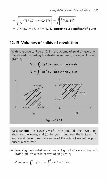
Integral Calculus and its Applications 347
� � � �15
737 87 0 46715
738 34[ . . ] [ . ]( ) ( )⎧⎨⎪⎪⎩⎪⎪
⎫⎬⎪⎪⎭⎪⎪
⎧⎨⎪⎪⎩⎪⎪
⎫⎬⎪⎪⎭⎭⎪⎪
� � �147 67 12 152. . 12.2, correct to 3 significant figures.
12.13 Volumes of solids of revolution
With reference to Figure 12.11 , the volume of solid of revolution V obtained by rotating the shaded area through one revolution is given by:
V y dx about the x-axis
V x dy about the y-axis
2a
b
2c
d
�
�
π
π
∫
∫
y
0
(a) (b)
0x � a
y � f (x)
x � f (y)
y � d
y
y � c
x � b x x
A
A
Figure 12.11
Application: The curve y � x 2 � 4 is rotated one revolution about (a) the x-axis, and (b) the y-axis, between the limits x � 1 and x � 4. Determine the volume of the solid of revolution pro-duced in each case
(a) Revolving the shaded area shown in Figure 12.12 about the x-axis 360° produces a solid of revolution given by:
Volume y dx (x ) dx� � �π π2
1
42 2
1
44∫ ∫
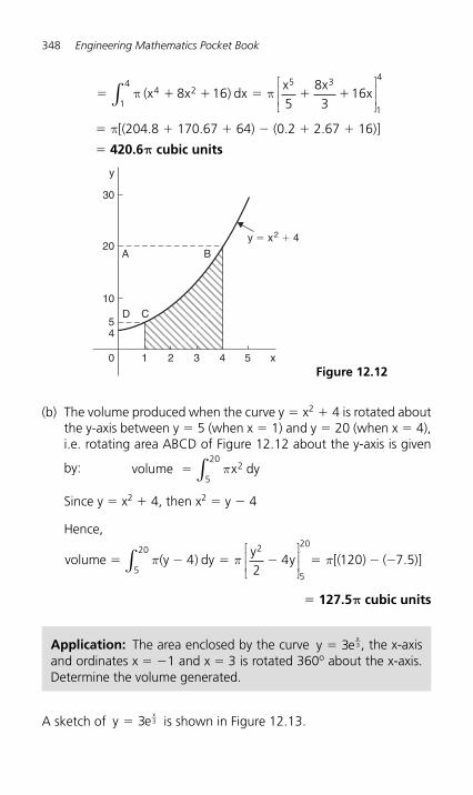
348 Engineering Mathematics Pocket Book
� � � � � �π π(x x ) dxx x
x4 21
4 5 3
1
4
8 165
83
16∫⎡
⎣⎢⎢
⎤
⎦⎥⎥
� π [(204.8 � 170.67 � 64) � (0.2 � 2.67 � 16)]
� 420.6π cubic units
Application: The area enclosed by the curve y e� 3 3x , the x-axis
and ordinates x � � 1 and x � 3 is rotated 360 o about the x-axis. Determine the volume generated.
30
20
10
54
0 1 2 3 4 5
y � x2 � 4
y
x
A B
CD
Figure 12.12
(b) The volume produced when the curve y � x 2 � 4 is rotated about the y-axis between y � 5 (when x � 1) and y � 20 (when x � 4), i.e. rotating area ABCD of Figure 12.12 about the y-axis is given
by: volume x dy� π 25
20
∫
Since y � x 2 � 4, then x 2 � y � 4
Hence,
volume (y ) dy
yy� � � � � � �π π π4
24 120 7 5
5
20 2
5
20
∫⎡
⎣⎢⎢
⎤
⎦⎥⎥ [( ) ( . )]
� 127.5π cubic units
A sketch of y e� 3 3x
is shown in Figure 12.13 .
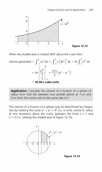
Integral Calculus and its Applications 349
When the shaded area is rotated 360 ° about the x-axis then:
volume generated y dx e dx e dx
e
� � �
�
� � �π π π
π
21
3 2
1
3
1
33 9
9
323∫ ∫ ∫( )x x
223 2
3
23
272
1
3
2x
⎡
⎣
⎢⎢⎢⎢⎢
⎤
⎦
⎥⎥⎥⎥⎥
( )�
�� �
�
πe e
92.82 cubic unitsπ
�2 0 2
x2 � y2 � 42
x
y
�4 1 43
Figure 12.14
8
4
0�1 21 3
y � 3e3x
y
x Figure 12.13
Application: Calculate the volume of a frustum of a sphere of radius 4 cm that lies between two parallel planes at 1 cm and 3 cm from the centre and on the same side of it
The volume of a frustum of a sphere may be determined by integra-tion by rotating the curve x 2 � y 2 � 4 2 (i.e. a circle, centre 0, radius 4) one revolution about the x-axis, between the limits x � 1 and x � 3 (i.e. rotating the shaded area of Figure 12.14 ).
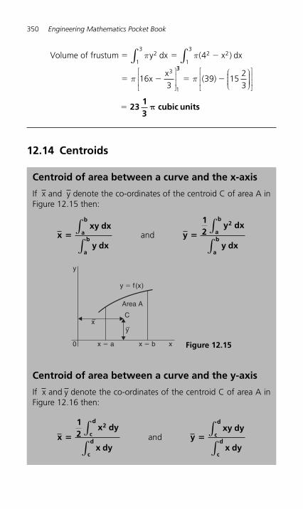
350 Engineering Mathematics Pocket Book
Volume of frustum y dx ( x ) dx
xx
� � �
� �
π π
π
21
32 2
1
3
3
1
4
163
∫ ∫⎡
⎣⎢⎢
⎤
⎦⎥⎥
33
39 1523
� �π ( )⎛⎝⎜⎜⎜
⎞⎠⎟⎟⎟⎟
⎡
⎣⎢⎢
⎤
⎦⎥⎥
� 23
13
cubic unitsπ
12.14 Centroids
Centroid of area between a curve and the x-axis
If x and y denote the co-ordinates of the centroid C of area A in Figure 12.15 then:
xxy dx
y dxy
12
y dx
y dx
a
b
a
b
2a
b
a
b� �∫∫
∫
∫and
Centroid of area between a curve and the y-axis
If x and y denote the co-ordinates of the centroid C of area A in Figure 12.16 then:
x
12
x dy
x dyy
xy dy
x dy
2c
d
c
dc
d
c
d� �∫
∫∫∫
and
y
0 x � a
x
x � b x
y � f (x)
C
Area A
y
Figure 12.15
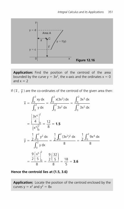
Integral Calculus and its Applications 351
If ( x , y ) are the co-ordinates of the centroid of the given area then:
x � � �
�
xy dx
y dx
x( x ) dx
3x dx
x dx
3x dx
x
0
22
0
22
0
20
22
0
23
0
2
4
3 3
34
∫∫
∫∫
∫∫
⎡
⎣⎣⎢⎢
⎤
⎦⎥⎥
⎡⎣⎢
⎤⎦⎥
∫
∫
0
2
20
2
0
2
2 20
2
128
12
12
3
x
yy dx
y dx
( x ) dx
30
2 � �
� �
1.5
∫∫ ∫
⎡
⎣⎢⎢
⎤
⎦⎥⎥
⎛⎝⎜⎜⎜
⎞⎠⎟⎟⎟⎟
8
12
9
92 5
8
92
325
8185
40
2
5
0
2
�
� � � �
x dx
8
x
3.6
Hence the centroid lies at (1.5, 3.6)
y
0
y � c
y � d
x
y � f (y)C
Area A
x
y
Figure 12.16
Application: Find the position of the centroid of the area bounded by the curve y � 3x 2, the x-axis and the ordinates x � 0 and x � 2
Application: Locate the position of the centroid enclosed by the curves y � x 2 and y 2 � 8x
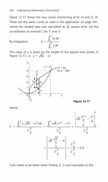
352 Engineering Mathematics Pocket Book
Figure 12.17 shows the two curves intersecting at (0, 0) and (2, 4).
These are the same curves as used in the application on page 341,
where the shaded area was calculated as 223 square units. Let the
co-ordinates of centroid C be x and y
By integration, x �xy dx
y dx
0
2
0
2
∫∫
The value of y is given by the height of the typical strip shown in Figure 12.17 , i.e. y x x� �8 2
2y
y
y C
y � x2
x2
4
3
2
1
0 1 2 x
y2 � 8x(or y � 8x)
Figure 12.17
Hence,
xx x x dx ( x x
x x
/
/
��
��
�
�
8
223
8
223
852
420
2
0
23 2 3
5 2 4
( )
⎡
⎣
⎢⎢⎢⎢⎢
⎤
⎦
⎥
∫ ∫ )
⎥⎥⎥⎥⎥
⎛
⎝
⎜⎜⎜⎜⎜⎜⎜⎜⎜⎜⎜⎜⎜⎜⎜⎜⎜
⎞
⎠
⎟⎟⎟⎟⎟⎟⎟⎟⎟⎟⎟⎟⎟⎟⎟⎟
0
2
5
223
8252
4
223
�
�
⎟⎟⎟⎟
� �2
25
223
0 9.
Care needs to be taken when finding y in such examples as this.
Integral Calculus and its Applications 353
From Figure 12.17 , y x x and y
x x� � � �82
12
82 2( )
The perpendicular distance from centroid C of the strip to OX is 12
8 2 2x x� �( ) x
Taking moments about 0x gives:
(total area) (y) (area of strip)(perpendicular distance of��
�
x
x
0
2
∑ centroid of strip to 0x))
Hence, (area) (y) x x x x x dx� � � �812
82 2 20
2 ⎡⎣⎢
⎤⎦⎥ ( )⎡
⎣⎢⎢
⎤
⎦⎥⎥∫
i.e. 223
882 2
20
2 2⎛⎝⎜⎜⎜
⎞⎠⎟⎟⎟⎟
⎡⎣⎢
⎤⎦⎥⎛
⎝⎜⎜⎜⎜
⎞
⎠⎟⎟⎟⎟⎟∫( )y x x
x xx� � � d
� � � �
� �
82 2
84 10
8 315
4
0
2 2 5
0
2x x
dxx x⎛
⎝⎜⎜⎜⎜
⎞
⎠⎟⎟⎟⎟
⎡
⎣⎢⎢
⎤
⎦⎥⎥
⎛⎝⎜⎜⎜
⎞⎠
∫⎟⎟⎟⎟⎟ � �( )0 4
45
Hence y � �4
45
223
1 8.
Thus the position of the centroid of the enclosed area in Figure 12.17 is at (0.9, 1.8)
Application: Locate the centroid of the area enclosed by the curve y � 2x 2, the y-axis and ordinates y � 1 and y � 4, correct to 3 decimal places
xx dy
x dy
ydy
dy
y
y� � �
12
12 2
2
12 4
23 2
21
4
1
41
4
1
4
2
1
4
3 2
∫
∫
∫
∫
⎡
⎣⎢⎢
⎤
⎦⎥⎥
⎡y /
⎣⎣⎢⎢
⎤
⎦⎥⎥1
4
158
143 2
0 568� � .
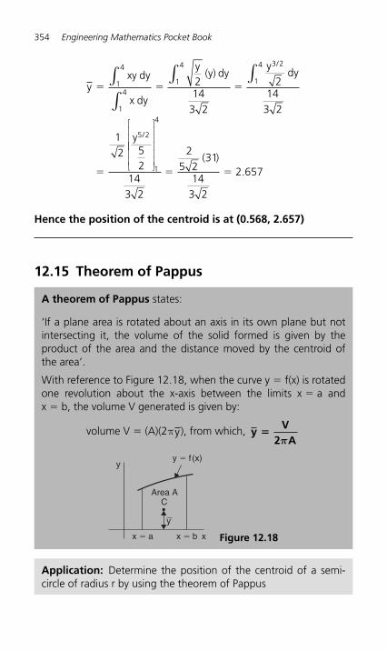
354 Engineering Mathematics Pocket Book
yxy dy
x dy
y(y) dy
ydy
y
/
/
� � �
�
1
4
1
41
4 3 2
1
4
5 2
214
3 2
214
3 2
12 5
2
∫∫
∫ ∫
⎡
⎣
⎢⎢⎢⎢⎢⎢
⎤
⎦
⎥⎥⎥⎥⎥1
4
143 2
25 2
31
143 2
2 657� �
( ).
Hence the position of the centroid is at (0.568, 2.657)
12.15 Theorem of Pappus
A theorem of Pappus states:
‘ If a plane area is rotated about an axis in its own plane but not intersecting it, the volume of the solid formed is given by the product of the area and the distance moved by the centroid of the area ’ .
With reference to Figure 12.18 , when the curve y � f(x) is rotated one revolution about the x-axis between the limits x � a and x � b, the volume V generated is given by:
volume V � (A)(2 π y ), from which, yV
2 A�π
Area A
y � f (x)
y
x
y
C
x � bx � a Figure 12.18
Application: Determine the position of the centroid of a semi-circle of radius r by using the theorem of Pappus
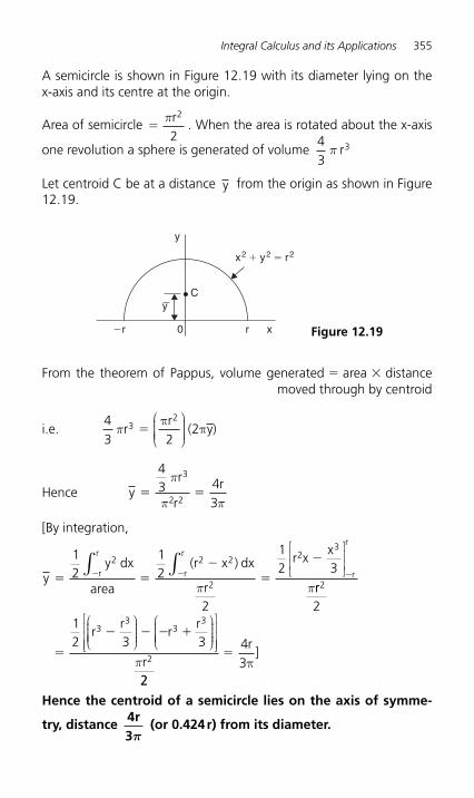
Integral Calculus and its Applications 355
A semicircle is shown in Figure 12.19 with its diameter lying on the x-axis and its centre at the origin.
Area of semicircle �πr2
2 . When the area is rotated about the x-axis
one revolution a sphere is generated of volume 43π r3
Let centroid C be at a distance y from the origin as shown in Figure 12.19 .
0�r r x
x2 � y2 � r2
y
Cy
Figure 12.19
From the theorem of Pappus, volume generated � area � distance moved through by centroid
i.e. 43 2
232
πrr
y)�π
π⎛
⎝⎜⎜⎜⎜
⎞
⎠⎟⎟⎟⎟ (
Hence yr
rr
� �
43 4
3
3
2 2
π
π π
[By integration,
yy dx
area
(r x ) dx
r
r xx
r
r
r
r
r
r
� ��
�
�� � �
12
12
2
12 3
2 2 2
2
23
∫ ∫⎡
⎣⎢⎢
⎤
⎦⎥⎥
π πrr
rr
rr
r
2
33
33
2
212 3 3
�
� � � �⎛
⎝⎜⎜⎜⎜
⎞
⎠⎟⎟⎟⎟
⎛
⎝⎜⎜⎜⎜
⎞
⎠⎟⎟⎟⎟
⎡
⎣⎢⎢⎢
⎤
⎦⎥⎥⎥
π22
43
�rπ
]
Hence the centroid of a semicircle lies on the axis of symme-
try, distance 4r3π
(or 0.424 r) from its diameter.
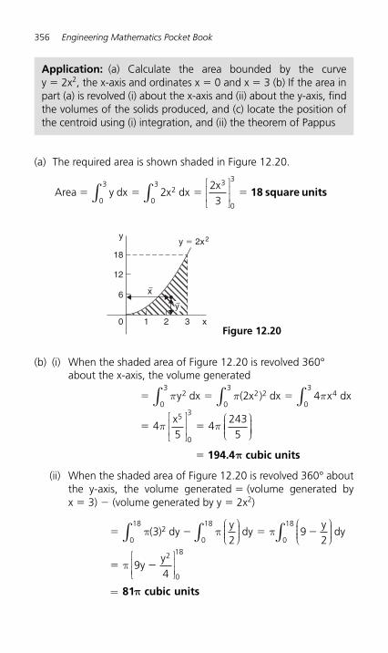
356 Engineering Mathematics Pocket Book
(a) The required area is shown shaded in Figure 12.20 .
Area y dx x dx
x� � � �
0
32
0
3 3
0
3
223∫ ∫
⎡
⎣⎢⎢
⎤
⎦⎥⎥ 18 square units
Application: (a) Calculate the area bounded by the curve y � 2x2, the x-axis and ordinates x � 0 and x � 3 (b) If the area in part (a) is revolved (i) about the x-axis and (ii) about the y-axis, find the volumes of the solids produced, and (c) locate the position of the centroid using (i) integration, and (ii) the theorem of Pappus
y
18
12
6
0 1 2 3
y � 2x2y
x
x Figure 12.20
(b) (i) When the shaded area of Figure 12.20 is revolved 360° about the x-axis, the volume generated
� � �
� �
π π π
π π
y dx ( x dx x dx
x
20
32 2
0
34
0
3
5
0
3
2 4
45
42435
∫ ∫ ∫⎡
⎣⎢⎢
⎤
⎦⎥⎥
⎛⎝⎜
)
⎜⎜⎜⎞⎠⎟⎟⎟⎟
� 194.4π cubic units
(ii) When the shaded area of Figure 12.20 is revolved 360 ° about the y-axis, the volume generated � (volume generated by x � 3) � (volume generated by y � 2x 2 )
� � � �
�
π π π
π
( )32
92
9
20
18
0
18
0
18dy
ydy
ydy
y
⎛⎝⎜⎜⎜
⎞⎠⎟⎟⎟
⎛⎝⎜⎜⎜
⎞⎠⎟⎟⎟∫∫ ∫
��y2
0
18
4
⎡
⎣⎢⎢
⎤
⎦⎥⎥
= 81 cubic unitsπ
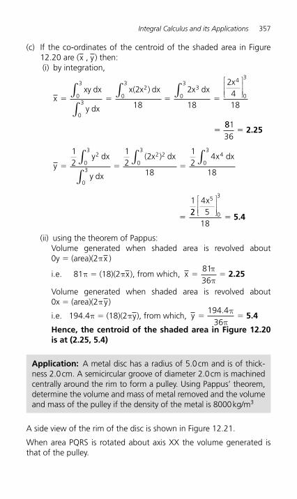
Integral Calculus and its Applications 357
(c) If the co-ordinates of the centroid of the shaded area in Figure 12.20 are ( x , y ) then:
(i) by integration,
xxy dx
y dx
x x dx x dxx
� � � �
�
0
3
0
3
20
33
0
3 4
0
3
2
18
2
18
2418
∫∫
∫ ∫⎡
⎣⎢⎢
⎤
⎦⎥⎥( )
88136
12
12
2
18
12
4
18
1
20
3
0
3
2 20
34
0
3
�
� � �
�
2.25
yy dx
y dx
x dx x dx∫
∫
∫ ∫( )
2245
18
5
0
3x⎡
⎣⎢⎢
⎤
⎦⎥⎥
� 5.4
(ii) using the theorem of Pappus: Volume generated when shaded area is revolved about 0y � (area)(2 π x )
i.e. 81 π � (18)(2 π x ), from which, x � �8136
ππ
2.25
Volume generated when shaded area is revolved about 0x � (area)(2 π y )
i.e. 194.4 π � (18)(2 π y ), from which, y � �194 4
36. ππ
5.4
Hence, the centroid of the shaded area in Figure 12.20 is at (2.25, 5.4)
Application: A metal disc has a radius of 5.0 cm and is of thick-ness 2.0 cm. A semicircular groove of diameter 2.0 cm is machined centrally around the rim to form a pulley. Using Pappus ’ theorem, determine the volume and mass of metal removed and the volume and mass of the pulley if the density of the metal is 8000 kg/m3
A side view of the rim of the disc is shown in Figure 12.21 .
When area PQRS is rotated about axis XX the volume generated is that of the pulley.
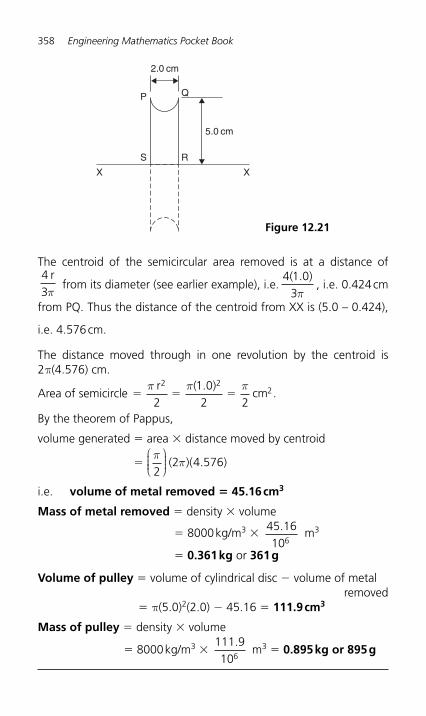
358 Engineering Mathematics Pocket Book
The centroid of the semicircular area removed is at a distance of 43
rπ
from its diameter (see earlier example), i.e. 4 1 0
3( . )π
, i.e. 0.424 cm
from PQ. Thus the distance of the centroid from XX is (5.0 – 0.424),
i.e. 4.576 cm.
The distance moved through in one revolution by the centroid is 2π (4.576) cm.
Area of semicircle � � �π πr
cm2 2
2
21 02 2
( . ) π .
By the theorem of Pappus,
volume generated � area � distance moved by centroid
�π
π2
2 4 576⎛⎝⎜⎜⎜
⎞⎠⎟⎟⎟ ( )( ).
i.e. volume of metal removed � 45.16 cm3
Mass of metal removed � density � volume
� 8000 kg/m 3 � 45 16106
. m 3
� 0.361 kg or 361 g
Volume of pulley � volume of cylindrical disc � volume of metal removed
� π (5.0) 2 (2.0) � 45.16 � 111.9 cm3
Mass of pulley � density � volume
� 8000 kg/m 3 � 111 9106
. m 3 � 0.895 kg or 895 g
5.0 cm
2.0 cm
P Q
RS
X X
Figure 12.21
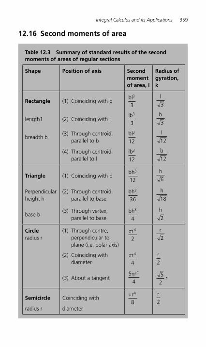
Integral Calculus and its Applications 359
12.16 Second moments of area
Table 12.3 Summary of standard results of the second moments of areas of regular sections
Shape Position of axis Second momentof area, I
Radius of gyration,k
Rectangle (1) Coinciding with b
bl3
3
l
3
length1 (2) Coinciding with l
lb3
3
b
3
breadth b (3) Through centroid,
parallel to b
bl3
12
l
12 (4) Through centroid,
parallel to l
lb3
12
b
12
Triangle (1) Coinciding with b
bh3
12
h
6
Perpendicular height h
(2) Through centroid, parallel to base
bh3
36
h
18
base b (3) Through vertex,
parallel to base
bh3
4
h
2
Circle radius r
(1) Through centre, perpendicular to plane (i.e. polar axis)
πr4
2
r
2
(2) Coinciding with diameter
πr4
4
r2
(3) About a tangent
54
4πr
52
r
Semicircle Coinciding with
πr4
8
r2
radius r diameter
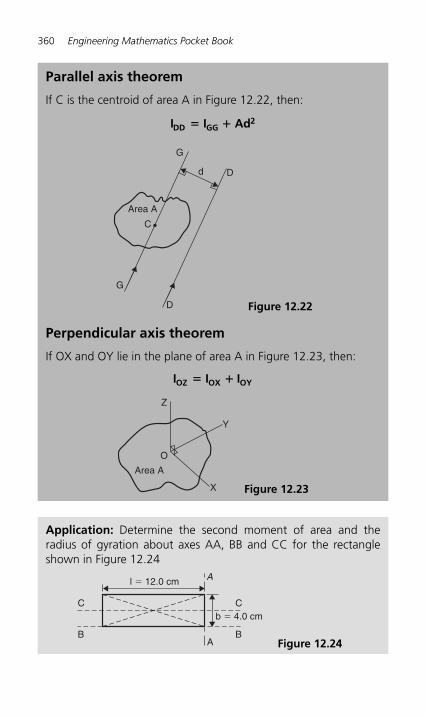
360 Engineering Mathematics Pocket Book
Parallel axis theorem
If C is the centroid of area A in Figure 12.22 , then:
I I AdDD GG2� �
Perpendicular axis theorem
If OX and OY lie in the plane of area A in Figure 12.23 , then:
I I IOZ OX OY� �
G
G
C
Area A
d D
D Figure 12.22
O
Area A
Z
Y
X Figure 12.23
Application: Determine the second moment of area and the radius of gyration about axes AA, BB and CC for the rectangle shown in Figure 12.24
A
C
B
Cb � 4.0 cm
BA
l � 12.0 cm
Figure 12.24
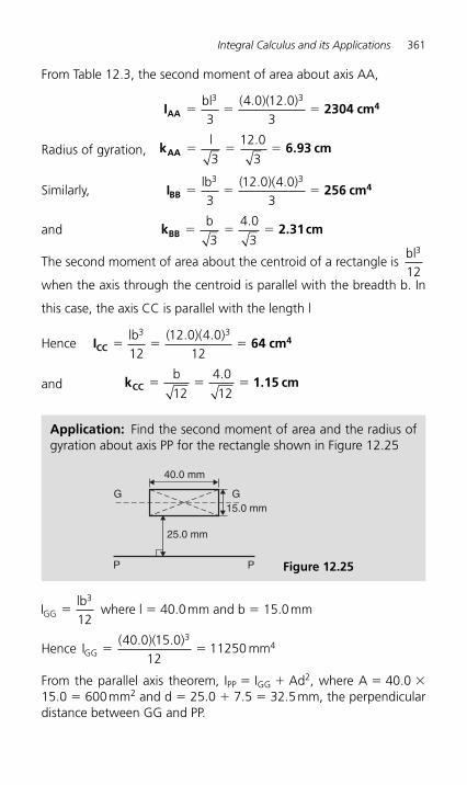
Integral Calculus and its Applications 361
Ib
GG �l 3
12 where l � 40.0 mm and b � 15.0 mm
Hence I mmGG � �( . )( . )40 0 15 0
1211250
34
From the parallel axis theorem, I PP � I GG � Ad 2, where A � 40.0 � 15.0 � 600 mm 2 and d � 25.0 � 7.5 � 32.5 mm, the perpendicular distance between GG and PP.
From Table 12.3 , the second moment of area about axis AA,
I 2304 cmAA4� � �
bl3 3
34 0 12 0
3( . )( . )
Radius of gyration, k 6.93 cmAA � � �l
3
12 0
3
.
Similarly, I 256 cmBB4� � �
lb3 3
312 0 4 0
3( . )( . )
and k 2.31cmBB � � �b
3
4 0
3
.
The second moment of area about the centroid of a rectangle is bl3
12
when the axis through the centroid is parallel with the breadth b. In
this case, the axis CC is parallel with the length l
Hence I 64 cmCC4� � �
lb3 3
1212 0 4 0
12( . )( . )
and kCC 1.15 cm� � �b
12
4 0
12
.
Application: Find the second moment of area and the radius of gyration about axis PP for the rectangle shown in Figure 12.25
40.0 mm
15.0 mm
25.0 mm
G G
P P Figure 12.25
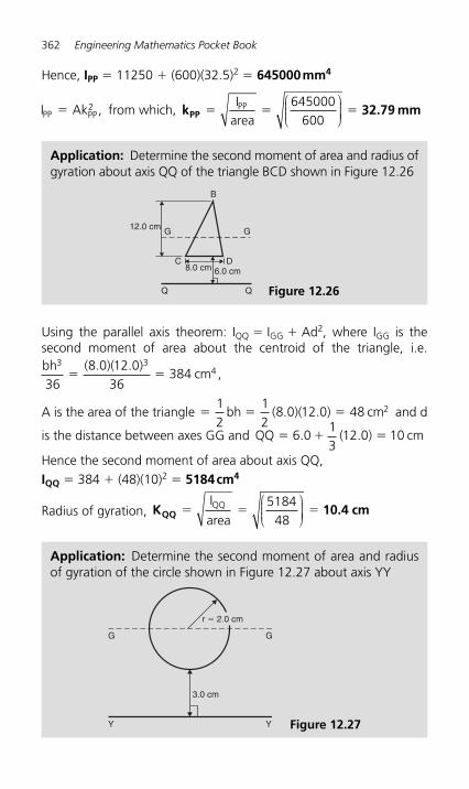
362 Engineering Mathematics Pocket Book
Hence, IPP � 11250 � (600)(32.5) 2 � 645000 mm4
I AkPP PP� 2 , from which, k 32.79 mmPP � � �I
areaPP 645000
600
⎛⎝⎜⎜⎜
⎞⎠⎟⎟⎟⎟
Application: Determine the second moment of area and radius of gyration about axis QQ of the triangle BCD shown in Figure 12.26
12.0 cm
8.0 cm 6.0 cm
B
G
DC
Q Q
G
Figure 12.26
Using the parallel axis theorem: I QQ � I GG � Ad2, where I GG is the second moment of area about the centroid of the triangle, i.e. bh
cm3 3
4
368 0 12 0
36384� �
( . )( . ) ,
A is the area of the triangle � � �12
12
8 0 12 0 48 2bh ( )( ) cm. . and d
is the distance between axes GG and QQ ( ) cm� � �6 013
12 0 10. .
Hence the second moment of area about axis QQ, IQQ � 384 � (48)(10) 2 � 5184 cm4
Radius of gyration, K 10.4 cmQQ � � �I
areaQQ 5184
48
⎛⎝⎜⎜⎜
⎞⎠⎟⎟⎟⎟
Application: Determine the second moment of area and radius of gyration of the circle shown in Figure 12.27 about axis YY
3.0 cm
G G
r � 2.0 cm
Y Y Figure 12.27
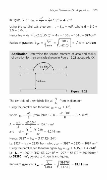
Integral Calculus and its Applications 363
In Figure 12.27 , IGG � � �π πr
( ) cm4
4 4
4 42 0 4. π
Using the parallel axis theorem, I YY � I GG � Ad2, where d � 3.0 � 2.0 � 5.0 cm.
Hence IYY � 4 π � [ π (2.0) 2 ](5.0) 2 � 4 π � 100 π � 104 π � 327 cm4
Radius of gyration, k 5.10 cmYY � � � �I
areaYY 104
2 026
2
ππ( . )
⎛
⎝⎜⎜⎜⎜
⎞
⎠⎟⎟⎟⎟
Application: Determine the second moment of area and radius of gyration for the semicircle shown in Figure 12.28 about axis XX
15.0 mm
10.0 mmG
B
G
B
XX Figure 12.28
The centroid of a semicircle lies at 43
rπ
from its diameter
Using the parallel axis theorem: I BB � I GG � Ad2 ,
where IBB �πr4
8 (from Table 12.3 ) � �
π( . )10 08
39274
4mm ,
A � � �
� � �
π
π π
rmm
and dr
mm
2 22
210 0
2157 1
43
4 10 03
4 244
π( . ).
( . ).
Hence, 3927 � I GG � (157.1)(4.244) 2
i.e. 3927 � IGG � 2830, from which, I GG � 3927 � 2830 � 1097 mm4
Using the parallel axis theorem again: I XX � I GG � A(15.0 � 4.244) 2
i.e. IXX � 1097 � (157.1)(19.244) 2 � 1097 � 58179 � 59276 mm 4 or 59280 mm4, correct to 4 significant figures.
Radius of gyration, k 19.42 mmXX � � �I
areaXX 59276
157 1.
⎛⎝⎜⎜⎜
⎞⎠⎟⎟⎟⎟
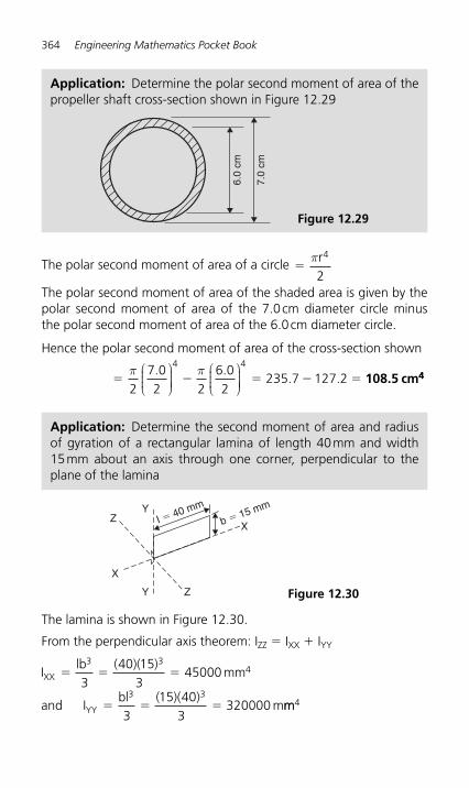
364 Engineering Mathematics Pocket Book
Y
Y Z
Xb � 15 mmI � 40 mm
Z
X
Figure 12.30
Application: Determine the polar second moment of area of the propeller shaft cross-section shown in Figure 12.29
7.0
cm
6.0
cm
Figure 12.29
The polar second moment of area of a circle �πr4
2
The polar second moment of area of the shaded area is given by the polar second moment of area of the 7.0 cm diameter circle minus the polar second moment of area of the 6.0 cm diameter circle.
Hence the polar second moment of area of the cross-section shown
� � � � �π2
7 02 2
6 02
235 7 127 24 4
. .. .
⎛⎝⎜⎜⎜
⎞⎠⎟⎟⎟⎟
⎛⎝⎜⎜⎜
⎞⎠⎟⎟⎟⎟
π108.5 cm44
Application: Determine the second moment of area and radius of gyration of a rectangular lamina of length 40 mm and width 15 mm about an axis through one corner, perpendicular to the plane of the lamina
The lamina is shown in Figure 12.30 .
From the perpendicular axis theorem: I ZZ � I XX � I YY
Il
l
XX � � �
� � �
bmm
and Ib
mYY
3 34
3 33
40 153
45000
315 40
3320000
( )( )
( )( )mm4
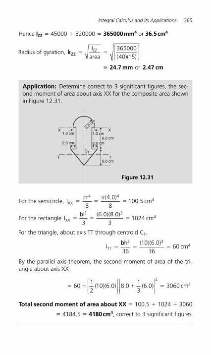
Integral Calculus and its Applications 365
Hence IZZ � 45000 � 320000 � 365000 mm 4 or 36.5 cm4
Radius of gyration, I
areaZZkZZ � �
36500040 15( )( )
⎛
⎝⎜⎜⎜⎜
⎞
⎠⎟⎟⎟⎟
�� 24.7 mm 2.47 cmor
For the semicircle, IXX � � �πr
cm4 4
4
84 08
100 5π( . )
.
For the rectangle Il
XX � � �b
cm3 3
4
36 0 8 0
31024
( . )( . )
For the triangle, about axis TT through centroid ,CT
�ITTbbh
cm3 3
4
3610 6 0
3660� �
( )( . )
By the parallel axis theorem, the second moment of area of the tri-angle about axis XX
� � � �6012
10 6 0 8 013
6 0 30602
4( )( . ) . ( . )⎡
⎣⎢⎢
⎤
⎦⎥⎥⎡
⎣⎢⎢
⎤
⎦⎥⎥
cm
Total second moment of area about XX � 100.5 � 1024 � 3060
� 4184.5 � 4180 cm 4 , correct to 3 significant figures
Application: Determine correct to 3 significant figures, the sec-ond moment of area about axis XX for the composite area shown in Figure 12.31 .
1.0 cm8.0 cm
6.0 cm
2.0 cm
4.0 cm
1.0 cm
2.0 cm
CT
TT
XX
Figure 12.31
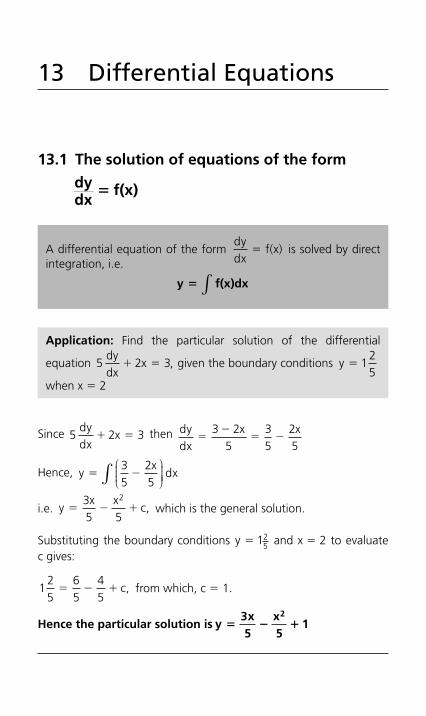
13.1 The solution of equations of the form
dydx
f(x)�
13 Differential Equations
Since 5 2 3dydx
x� � then dydx
x x�
�� �
3 25
35
25
Hence, yx
dx� �35
25
⎛⎝⎜⎜⎜
⎞⎠⎟⎟⎟⎟∫
i.e. yx x
c,� � �35 5
2 which is the general solution.
Substituting the boundary conditions y � 125 and x � 2 to evaluate
c gives:
125
65
45
� � � c, from which, c � 1.
Hence the particular solution is y3x5
x5
12
� � �
A differential equation of the form dydx
f(x)� is solved by direct integration, i.e.
y f(x)dx� ∫
Application: Find the particular solution of the differential
equation 5 2 3dydx
x� � , given the boundary conditions y 125
�
when x � 2
Differential Equations 367
13.2 The solution of equations of the form dydx
f(y)�
A differential equation of the form dydx
f(y)� is initially rearranged
to give dxdyf(y)
� and then the solution is obtained by direct
integration, i.e.
dxdyf(y)∫ ∫�
(a) dRd
Rθ
α� is of the form dydx
f(y)�
Rearranging gives: ddR
Rθ
α�
Integrating both sides gives: ddR
Rθ
α∫ ∫�
i.e. θα
� �1
ln R c, which is the general solution
Substituting the boundary conditions R � R 0 when θ � 0 gives:
01 1
0 0� � � �α α
ln R c from which c ln R
Application:
(a) The variation of resistance, R ohms, of an aluminium conductor
with temperature θ°C is given by dRd
R,θ
α� where α is the
temperature coefficient of resistance of aluminium. If R � R 0 when θ � 0°C, solve the equation for R.
(b) If α � 38 � 10 � 4/°C, determine the resistance of an alumin-ium conductor at 50°C, correct to 3 significant figures, when its resistance at 0°C is 24.0 Ω
368 Engineering Mathematics Pocket Book
Hence the particular solution is
θα α α
� � � �1 1 1
0 0ln R ln R (ln R ln R )
i.e. θα
αθ� �1
0 0
lnRR
or lnRR
⎛
⎝⎜⎜⎜⎜
⎞
⎠⎟⎟⎟⎟⎟
⎛
⎝⎜⎜⎜⎜
⎞
⎠⎟⎟⎟⎟⎟
Hence eRR
αθ �0
from which, R � R 0 e α θ
(b) Substituting α � 38 � 10 � 4, R 0 � 24.0 and θ � 50 into R � R0 e α θ gives the resistance at 50°C, i.e.
R50 � 24.0 e( )38 10 504� ��� 29.0 ohms
13.3 The solution of equations of the formdydx
f(x) . f(y)�
A differential equation of the form dydx
f(x).f(y),� where f(x) is
a function of x only and f(y) is a function of y only, may be
rearranged as dyf(y)
f(x)dx,� and then the solution is obtained
by direct integration, i.e.
dyf(y)
f(x)dx∫ ∫�
Application: Solve the equation 4xydydx
y 12� �
Separating the variables gives: 4
11
2
yy
dyx
dx�
�⎛
⎝⎜⎜⎜⎜
⎞
⎠⎟⎟⎟⎟
Differential Equations 369
Integrating both sides gives: 4
11
2
yy
dyx
dx�
�⎛
⎝⎜⎜⎜⎜
⎞
⎠⎟⎟⎟⎟
⎛⎝⎜⎜⎜
⎞⎠⎟⎟⎟⎟∫ ∫
Using the substitution u � y 2 � 1, the general solution is:
2 ln (y 1) ln x c2 � � � (1)
or ln (y 2 � 1) 2 � ln x � c
from which, ln(y )
xc
2 21��
⎧⎨⎪⎪⎩⎪⎪
⎫⎬⎪⎪⎭⎪⎪
and (y 1)
xe
2 2c�
�(2)
If in equation (1), c � ln A, where A is a different constant,
then ln (y2 � 1) 2 � ln x � ln A
i.e. ln (y2 � 1) 2 � ln Ax
i.e. (y 1) Ax2 2� � (3)
Equations (1) to (3) are thus three valid solutions of the differential
equations 4 12xydydx
y� �
Application: The current i in an electric circuit containing resistance R and inductance L in series with a constant voltage
source E is given by the differential equation E Ldidt
Ri.� �⎛⎝⎜⎜⎜
⎞⎠⎟⎟⎟⎟
Solve the equation to find i in terms of time t, given that when t � 0, i � 0
In the R–L series circuit shown in Figure 13.1 , the supply p.d., E, is given by
E V VR L� �
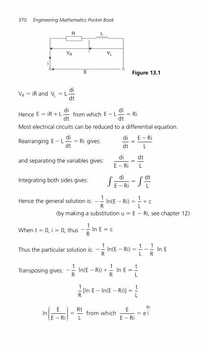
370 Engineering Mathematics Pocket Book
V R � iR and V LdidtL �
Hence E iR Ldidt
� � from which E Ldidt
Ri� �
Most electrical circuits can be reduced to a differential equation.
Rearranging E Ldidt
Ri� � gives: didt
E RiL
��
and separating the variables gives: diE Ri
dtL�
�
Integrating both sides gives: diE Ri
dtL�
�∫ ∫
Hence the general solution is: � � � �1R
ln(E Ri)tL
c
(by making a substitution u � E � Ri, see chapter 12)
When t � 0, i � 0, thus � �1R
ln E c
Thus the particular solution is: � � � �1 1R
ln(E Ri)tL R
ln E
Transposing gives: � � � �1 1R
ln(E Ri)R
ln EtL
1R
[ln E ln(E Ri)]tL
� � �
lnE
E RiRtL
from which E
E Rie
RtL
��
��
⎛⎝⎜⎜⎜
⎞⎠⎟⎟⎟⎟
VR VL
R L
E
i
Figure 13.1
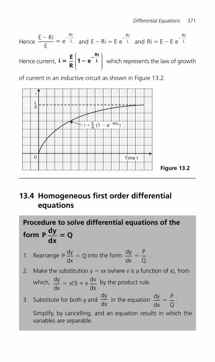
Differential Equations 371
Hence E Ri
Ee
RtL
��
�
and E Ri E eRtL� �
� and Ri E E e
RtL� �
�
Hence current, iER
1 eRtL� �
�⎛
⎝⎜⎜⎜⎜⎜
⎞
⎠
⎟⎟⎟⎟⎟ which represents the law of growth
of current in an inductive circuit as shown in Figure 13.2 .
i
i � (1 � e�Rt/L)
Time t0
ER
ER
Figure 13.2
13.4 Homogeneous first order differential equations
Procedure to solve differential equations of the
form Pdydx
Q�
1. Rearrange Pdydx
Q� into the form dydx
PQ
� .
2. Make the substitution y � vx (where v is a function of x), from
which, dydx
v( ) xdvdx
� �1 by the product rule.
3. Substitute for both y and dydx
in the equation dydx
PQ
.�
Simplify, by cancelling, and an equation results in which the variables are separable.
372 Engineering Mathematics Pocket Book
Using the above procedure:
1. Rearranging xdydx
x yy
��2 2
gives dydx
x yxy
��2 2
which is
homogeneous in x and y since each of the three terms on the
right hand side are of the same degree (i.e. degree 2).
2. Let y � vx then dydx
v( ) xdvdx
� �1
3. Substituting for y and dydx
in the equation dydx
x yxy
��2 2
gives:
v xdvdx
x (vx)x(vx)
x v xvx
vv
� � ��
��2 2 2 2 2
2
21+
4. Separating the variables give:
xdvdx
vv
vv v
v v�
�� �
� ��
1 1 12 2 2
Hence, vdvx
dx�1
Integrating both sides gives:
vdvx
dx�1
∫∫ i.e. v ln x c2
2� �
4. Separate the variables and solve.
5. Substitute vyx
� to solve in terms of the original variables.
Application: Determine the particular solution of the equation
xdydx
x yy
,2 2
�� given the boundary conditions that x � 1 when
y � 4
Differential Equations 373
5. Replacing v byyx
gives:yx
ln x c,2
22� � which is the general
solution.
When x � 1, y � 4, thus: 162
1� �ln c, from which, c � 8
Hence, the particular solution is: y2x
ln x 82
2� � or
y2 � 2x 2 (ln x � 8)
13.5 Linear first order differential equations
Procedure to solve differential equations of the
formdydx
Py Q� �
1. Rearrange the differential equation into the form
dydx
Py Q,� � where P and Q are functions of x
2. Determine P dx∫
3. Determine the integrating factor e P dx∫
4. Substitute e P dx∫ into the equation:
y e e Q dxP dx P dx∫ ∫∫� (1)
5. Integrate the right hand side of equation (1) to give the gen-eral solution of the differential equation. Given boundary con-ditions, the particular solution may be determined.
374 Engineering Mathematics Pocket Book
Using the above procedure:
1. Rearranging gives dydx
xy x,+ 4 2� which is of the form
dydx
Py Q� � where P � 4x and Q � 2x
2. P dx x dx x∫ ∫� �4 2 2
3. Integrating factor, e P dx∫ � e x2 2
4. Substituting into equation (1) gives:
y e e ( x) dxx x2 22 2 2� ∫
5. Hence the general solution is: y e e c,x x2 22 212
� � by using the
substitution u � 2x 2
When x � 0, y � 4, thus 412
0 0e e c,� � from which, c �72
Hence the particular solution is:
y e ex x2 22 212
72
� �
i.e. y12
72
e 2x2� � � or y
12
(1 7e )2x2� � �
Application: Solve the differential equation 1x
dydx
4y 2� � ,
given the boundary conditions x � 0 when y � 4
Differential Equations 375
13.6 Second order differential equations of the
form a d ydx
b dydx
cy 02
2 � � �
Procedure to solve differential equations of the form
ad ydx
bdydx
cy 02
2� � �
1. Rewrite the differential equation ad ydx
bdydx
cy 02
2� � � as
(aD2 � bD � c)y � 0
2. Substitute m for D and solve the auxiliary equation am2 � bm � c � 0 for m
3. If the roots of the auxiliary equation are: (a) real and different, say m � α and m � β, then the gen-
eral solution is: y � Aeαx � Be βx (b) real and equal, say m � α twice, then the general solu-
tion is: y � (Ax � B)e αx (c) complex, say m � α j β, then the general solution is:
y � e αx { A cos β x � B sin β x } 4. Given boundary conditions, constants A and B may be deter-
mined and the particular solution of the differential equation obtained. The particular solution obtained with differential equations may be verified by substituting expressions for y,
dydx
and d ydx
2
2 into the original equation.
Application: The oscillations of a heavily damped pendulum
satisfy the differential equation d xdt
6dxdt
8x 02
2� � � , where x
cm is the displacement of the bob at time t seconds.
The initial displacement is equal to � 4 cm and the initial velocity
i.e.dxdt
⎛⎝⎜⎜⎜
⎞⎠⎟⎟⎟⎟ is 8 cm/s. Solve the equation for x.
376 Engineering Mathematics Pocket Book
Using the above procedure:
1. d xdt
dxdt
x2
26 8 0� � � in D-operator form is (D 2 � 6D � 8)x � 0,
where Dddt
≡
2. The auxiliary equation is m 2 � 6 m � 8 � 0 Factorising gives: (m � 2)(m � 4) � 0, from which, m � � 2 or m � � 4
3. Since the roots are real and different, the general solution is:
x Ae Be2t 4t� �� �
4. Initial displacement means that time t � 0. At this instant, x � 4
Thus 4 � �A B (1)
Velocity, dxdt
Ae Bet t� � �� �2 42 4
dxdt
cm/s� 8 when t � 0, thus 8 � �2A � 4B (2)
From equations (1) and (2), A � 12 and B � � 8
Hence the particular solution is: x � 12e � 2t � 8e � 4t
i.e. displacement, x � 4(3e � 2t � 2e � 4t ) cm
Application: The equation d idt
RL
didt
1LC
i 02
2� � � represents
a current i flowing in an electrical circuit containing resistance R, inductance L and capacitance C connected in series. If R � 200 ohms, L � 0.20 henry and C � 20 � 10 � 6 farads, solve the equation for i given the boundary conditions that when t � 0,
i � 0 and didt
100�
Differential Equations 377
Using the procedure:
1. d idt
RL
didt LC
i2
2
10� � � in D-operator form is
DRL
DLC
i2 10� � �
⎛⎝⎜⎜⎜
⎞⎠⎟⎟⎟⎟ where D
ddt
≡
2. The auxiliary equation is mRL
mLC
2 10� � �
Hence, m
( )LC
�
� �RL
RL
±⎛⎝⎜⎜⎜
⎞⎠⎟⎟⎟⎟
⎛⎝⎜⎜⎜
⎞⎠⎟⎟⎟⎟
⎡
⎣
⎢⎢⎢
⎤
⎦
⎥⎥⎥
2
4 11
2
When R � 200, L � 0.20 and C � 20 � 10 � 6 ,
then m( )( )
�
� �� �
2000 20
2000 20
40 20 20 10
2
2
6. . .±
⎛⎝⎜⎜⎜
⎞⎠⎟⎟⎟⎟
⎡
⎣
⎢⎢⎢
⎤
⎦
⎥⎥⎥
���
� �1000 0
2500
±
3. Since the two roots are real and equal (i.e. �500 twice, since for a second order differential equation there must be two solutions), the general solution is: i � (At � B)e � 500 t
4. When t � 0, i � 0, hence B � 0
didt
(At B)( e ) (e )(A)� � � �� �500 500 500t t by the product rule
When t , didt
,� �0 100 thus 100 � � 500B � A
i.e. A � 100, since B � 0
Hence the particular solution is: i � 100 te � 500 t
378 Engineering Mathematics Pocket Book
An equation of the form d xdt
m x2
22 0� � is a differential equation
representing simple harmonic motion (S.H.M.). Using the procedure:
1. d xdt
x2
2100 0� � in D-operator form is (D 2 � 100)x � 0
2. The auxiliary equation is m 2 � 100 � 0, i.e. m 2 � � 100 and
m � �100 i.e. m � j10
3. Since the roots are complex, the general solution is: x � e 0 (A cos 10 t � B sin 10 t),
i.e. x � (A cos 10 t � B sin 10 t) metres
4. When t � 0, x � 2, thus 2 � A
dxdt
A� �10 sin 10t � 10B cos 10t
When t � 0, dxdt
� 0 thus 0 � � 10A sin 0 � 10B cos 0 i.e. B � 0
Hence the particular solution is: x � 2 cos 10t metres
Application: The equation of motion of a body oscillating on
the end of a spring isd xdt
100x 0,2
2� � where x is the
displacement in metres of the body from its equilibrium position after time t seconds. Determine x in terms of t given that at time
t � 0, x � 2 m and dxdt
0�
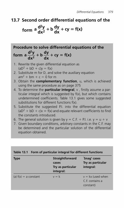
Differential Equations 379
13.7 Second order differential equations of the
form a d ydx
b dydx
cy f(x)2
2 � � �
Procedure to solve differential equations of the
form ad ydx
bdydx
cy f(x)2
2� � �
1. Rewrite the given differential equation as (aD2 � bD � c)y � f(x)
2. Substitute m for D, and solve the auxiliary equation am2 � bm � c � 0 for m
3. Obtain the complementary function, u, which is achieved using the same procedure as on page 375
4. To determine the particular integral, v , firstly assume a par-ticular integral which is suggested by f(x), but which contains undetermined coefficients. Table 13.1 gives some suggested substitutions for different functions f(x).
5. Substitute the suggested P.I. into the differential equation (aD2 � bD � c)v � f(x) and equate relevant coefficients to find the constants introduced.
6. The general solution is given by y � C.F. � P.I. i.e. y � u � v7. Given boundary conditions, arbitrary constants in the C.F. may
be determined and the particular solution of the differential equation obtained.
Table 13.1 Form of particular integral for different functions
Type Straightforward casesTry as particular integral:
‘Snag’ cases Try as particular integral:
(a) f(x) � a constant v � k v � kx (used when C.F. contains a constant)
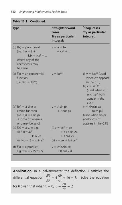
380 Engineering Mathematics Pocket Book
Table 13.1 Continued
Type Straightforward casesTry as particular integral:
‘Snag’ cases Try as particular integral:
(b) f(x) � polynomial (i.e. f(x) � L � Mx � Nx2 � .. where any of the coefficients may be zero)
v � a � bx � cx2 � ..
(c) f(x) � an exponential function(i.e. f(x) � Aeax)
v � keax (i) v � kxeax (usedwhen eax appears in the C.F.)
(ii) v � kx2eax
(used when eax
and xeax both appear in the C.F.)
(d) f(x) � a sine or cosine function (i.e. f(x) � a sin px � b cos px where a or b may be zero)
v � A sin px � B cos px
v � x(A sin px � B cos px)
(used when sin px and/or cos px appears in the C.F.)
(e) f(x) � a sum e.g. (i) f(x) � 4x2
� 3 sin 2x (ii) f(x) � 2 � x � e3x
(i) v � ax2 � bx � c�d sin 2x � e cos 2x(ii) v � ax � b�ce3x
(f) f(x) � a producte.g. f(x) � 2excos 2x
v � ex(A sin 2x � B cos 2x)
Application: In a galvanometer the deflection θ satisfies the
differential equation d4 4
2θ θθ
dtddt
.2
8� � � Solve the equation
for θ given that when t � 0, θθ
� �ddt
2
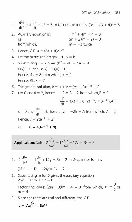
Differential Equations 381
1.ddt
4ddt
2
24 8
θ θθ� � � in D-operator form is: (D2 � 4D � 4)θ � 8
2. Auxiliary equation is: m2 � 4m � 4 � 0 i.e. (m � 2)(m � 2) � 0 from which, m � �2 twice
3. Hence, C.F., u � (At � B)e�2t
4. Let the particular integral, P.I., v � k
5. Substituting v � k gives: (D2 � 4D � 4)k � 8
D(k) � 0 and D2(k) � D(0) � 0
Hence, 4k � 8 from which, k � 2
Hence, P.I., v � 2
6. The general solution, θ � u � v � (At � B)e�2t � 2
7. t � 0 and θ � 2, hence, 2 � B � 2 from which, B � 0
ddt
(At B)( e ) (e )(A)t tθ� � � �� �2 2 2
x � 0 and ddt
,θ
� 2 hence, 2 � �2B � A from which, A � 2
Hence, θ � 2te�2t � 2
i.e. θ � 2(te�2t � 1)
Application: Solve 2 11 12 3 22
2
d ydx
dydx
y x� � � �
1. 2 11 12 3 22
2
d ydx
dydx
y x� � � � in D-operator form is
(2D2 � 11D � 12)y � 3x � 2
2. Substituting m for D gives the auxiliary equation 2m2 � 11m � 12 � 0
Factorising gives: (2m � 3)(m � 4) � 0, from which, m �32
orm � 4
3. Since the roots are real and different, the C.F.,
u Ae Be32
x 4x� �
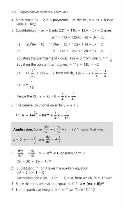
382 Engineering Mathematics Pocket Book
4. Since f(x) � 3x � 2 is a polynomial, let the P.I., v � ax � b (see Table 13.1(b))
5. Substituting v � ax � b into (2D2 � 11D � 12)v � 3x � 2 gives:
( D D )(ax b) x 2,2 11 12 32 � � � �+
i.e. 2D2(ax � b) � 11D(ax � b) � 12(ax � b) � 3x � 2
i.e. 0 � 11a � 12ax � 12b � 3x � 2
Equating the coefficients of x gives: 12a � 3, from which, a �14
Equating the constant terms gives: � 11a � 12b � �2
i.e. � � � �11 b 214
12⎛⎝⎜⎜⎜
⎞⎠⎟⎟⎟⎟ from which, 12 2
114
34
b � � � �
i.e. b �1
16
Hence the P.I., v14
x1
16� � �ax b �
6. The general solution is given by y � u � v
i.e. y Ae Be14
x1
16
32
x 4x� � � �
Application: Solve d ydx
dydx
y e x2
242 3� � � given that when
x � 0, y � �23
and dydx
� 413
1.d ydx
dydx
y e x2
242 3� � � in D-operator form is
(D2 � 2D � 1)y � 3e4x
2. Substituting m for D gives the auxiliary equation m2 � 2m � 1 � 0
Factorising gives: (m � 1)(m � 1) � 0, from which, m � 1 twice
3. Since the roots are real and equal the C.F., u � (Ax � B)ex
4. Let the particular integral, v � ke4x (see Table 13.1(c))
Differential Equations 383
5. Substituting v � ke4x into (D2 � 2D � 1)v � 3e4x gives:
(D D )ke ex x2 4 42 1 3� � �
i.e. D (ke ) D(ke ) (ke ex x x x2 4 4 4 42 1 3� � �)
i.e. 16ke4x � 8ke4x � ke4x � 3e4x
Hence 9ke4x � 3e4x, from which, k �13
Hence the P.I., v � ke4x �13
e4x
6. The general solution is given by y � u � v, i.e.
y (Ax B)e13
ex 4x� � �
7. When x � 0, y � �23
thus � � � �23
013
0 0( B)e e , from
which, B � �1
dydx
(Ax B)e e (A) ex x x� � � �43
4
When x � 0, dydx
,� 413
thus 133
43
� � �B A from
which, A � 4, since B � �1
Hence the particular solution is: y (4x 1)e13
ex 4x� � �
Application: Ld qdt
Rdqdt
1C
q V sin wt2
2 0� � � represents the
variation of capacitor charge in an electric circuit. Determine an expression for q at time t seconds given that R � 40 Ω,L � 0.02 H, C � 50 � 10 �6 F, V0 � 540.8 V and ω � 200 rad/s and given the boundary conditions that when t � 0, q � 0 anddqdt
4.8�
384 Engineering Mathematics Pocket Book
Ld qdt
Rdqdt C
q V2
2 01
� � � �sin t in D-operator form is:
L D R DC
q V t20
1� � � �
⎛⎝⎜⎜⎜
⎞⎠⎟⎟⎟⎟ sin
The auxiliary equation is: L m R mC
2 10� � �
and
mR R
LC
L�
� �
�
� ��
��
� ��
2 26
4
2
40 404 0 02
50 102 0 02
40 00 04
100
( . )
( . ) .00
Hence, C.F., u � (At � B)e�1000t
Let P.I., v � A sin ωt � B cos ωt
L D R DC
[A B t] V t20
1� � � � � � �
⎛⎝⎜⎜⎜
⎞⎠⎟⎟⎟⎟ sin cos sint
D(v) � Aω cos ωt�Bω sin ωt and D2(v) � �Aω2 sin ωt � Bω2 cos ωt
Thus,
L D R DC
2 1� �
⎛⎝⎜⎜⎜
⎞⎠⎟⎟⎟⎟v � 0.02(�Aω2 sin ωt � Bω2 cos ωt)
� 40 (Aω cos ωt � Bω sin ωt)
�1
50 10 6� � (A sin ωt �B cos ωt) � V0 sin ωt
i.e. �800A sin 200t � 800B cos 200t � 8000A cos 200t �8000B sin 200t � 20000A sin 200t � 20000B cos 200t � 540.8 sin 200t
Hence, �800A � 8000B � 20000A � 540.8
and �800B � 8000A � 20000B � 0
i.e. 19200 8000 540 8A B� � . (1)
and 8000 19200 0A B� � (2)
8 � (1) gives: 153600 64000 4326 4A B� � . (3)
19.2 � (2) gives: 153600 368640 0A B� � (4)
(3)–(4) gives: �432640B � 4326.4
Differential Equations 385
from which, B � � �4326 4432640
0 01.
.
Substituting in (1) gives: 19200A � 8000(�0.01) � 540.8
i.e. 19200A � 80 � 540.8
and A ��
�540 8 80
19200460 819200
0 024. .
.=
Hence, P.I., v � 0.024 sin 200t – 0.01 cos 200t
Thus, q � u � v � (At � B)e�1000t � 0.024 sin 200t � 0.01 cos 200t
When t � 0, q � 0, hence, 0 � B � 0.01 from which, B � 0.01
dqdt
(At B) e Ae ( )( ) tt t� � � � �
� �1000 0 024 200 2001000 1000( ) . cos
� ( )( ) t0 01 200 200. sin
When t � 0, dqdt
,� 4 8. hence, 4.8 � �1000B � A � 4.8
i.e. A � 1000B � 1000(0.01) � 10
Thus, q � (10t � 0.01)e�1000t � 0.024 sin 200t � 0.010 cos 200t
13.8 Numerical methods for first order differential equations
Euler’s method
y y h(y )1 0 0� � � (1)
Application: Obtain a numerical solution of the differential
equation dydx
3(1 x) y� � � given the initial conditions that
x � 1 when y � 4, for the range x � 1.0 to x � 2.0 with intervals of 0.2.
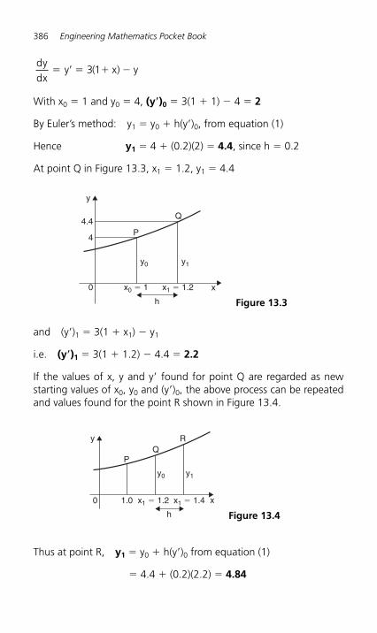
386 Engineering Mathematics Pocket Book
dydx
y ( x) y� � � � �3 1
With x0 � 1 and y0 � 4, (y�)0 � 3(1 � 1) � 4 � 2
By Euler’s method: y1 � y0 � h(y�)0, from equation (1)
Hence y1 � 4 � (0.2)(2) � 4.4, since h � 0.2
At point Q in Figure 13.3, x1 � 1.2, y1 � 4.4
P
0
4
4.4Q
y
y0
x0 � 1 x1 � 1.2
y1
x
h Figure 13.3
and (y�)1 � 3(1 � x1) � y1
i.e. (y�)1 � 3(1 � 1.2) � 4.4 � 2.2
If the values of x, y and y� found for point Q are regarded as new starting values of x0, y0 and (y�)0, the above process can be repeated and values found for the point R shown in Figure 13.4.
PQ
0 1.0
Ry
y0
x1 � 1.2 x1 � 1.4
y1
x
h Figure 13.4
Thus at point R, y1 � y0 � h(y�)0 from equation (1)
� 4.4 � (0.2)(2.2) � 4.84
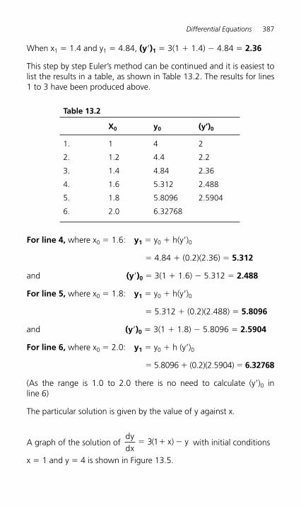
Differential Equations 387
When x1 � 1.4 and y1 � 4.84, (y�)1 � 3(1 � 1.4) � 4.84 � 2.36
This step by step Euler’s method can be continued and it is easiest to list the results in a table, as shown in Table 13.2. The results for lines 1 to 3 have been produced above.
Table 13.2
X0 y0 (y’)0
1. 1 4 2
2. 1.2 4.4 2.2
3. 1.4 4.84 2.36
4. 1.6 5.312 2.488
5. 1.8 5.8096 2.5904
6. 2.0 6.32768
For line 4, where x0 � 1.6: y1 � y0 � h(y�)0
� 4.84 � (0.2)(2.36) � 5.312
and (y�)0 � 3(1 � 1.6) � 5.312 � 2.488
For line 5, where x0 � 1.8: y1 � y0 � h(y�)0
� 5.312 � (0.2)(2.488) � 5.8096
and (y�)0 � 3(1 � 1.8) � 5.8096 � 2.5904
For line 6, where x0 � 2.0: y1 � y0 � h (y�)0
� 5.8096 � (0.2)(2.5904) � 6.32768
(As the range is 1.0 to 2.0 there is no need to calculate (y�)0 in line 6)
The particular solution is given by the value of y against x.
A graph of the solution of dydx
( x) y� � �3 1 with initial conditions
x � 1 and y � 4 is shown in Figure 13.5.
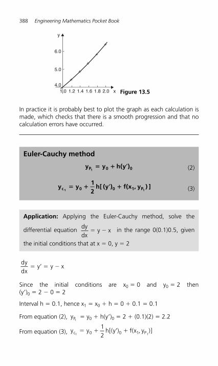
388 Engineering Mathematics Pocket Book
In practice it is probably best to plot the graph as each calculation is made, which checks that there is a smooth progression and that no calculation errors have occurred.
y
x1.04.0
5.0
6.0
1.2 1.4 1.6 1.8 2.0 Figure 13.5
Euler-Cauchy method
y y h(y )P 0 01� � � (2)
y y12
h[ (y ) f(x , y ) ]c 0 0 1 P1 1� � � � (3)
Application: Applying the Euler-Cauchy method, solve the
differential equation dydx
y x� � in the range 0(0.1)0.5, given
the initial conditions that at x � 0, y � 2
dydx
y y x� � � �
Since the initial conditions are x0 � 0 and y0 � 2 then (y�)0 � 2 � 0 � 2
Interval h � 0.1, hence x1 � x0 � h � 0 � 0.1 � 0.1
From equation (2), yP1� y0 � h(y�)0 � 2 � (0.1)(2) � 2.2
From equation (3), y y h[(y ) f(x , y )]c P1 10 0 112
� � � �
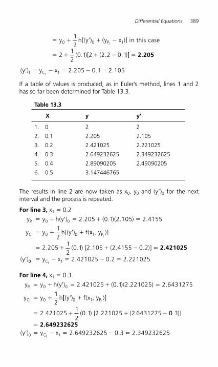
Differential Equations 389
� � � � �
� � � �
y h[(y ) (y x )] in this case
( )[ ( )
P0 0 112
212
0 1 2 2 2 0 1
1
. . . ]] � 2.205
(y ) y xC� � � � � �1 112 205 0 1 2 105. . .
If a table of values is produced, as in Euler’s method, lines 1 and 2 has so far been determined for Table 13.3.
Table 13.3
X y y’
1. 0 2 2
2. 0.1 2.205 2.105
3. 0.2 2.421025 2.221025
4. 0.3 2.649232625 2.349232625
5. 0.4 2.89090205 2.49090205
6. 0.5 3.147446765
The results in line 2 are now taken as x0, y0 and (y�)0 for the next interval and the process is repeated.
For line 3, x1 � 0.2
y y h(y ) ( )( )
y y h[(y ) f(
P
C
1
1
0 0
0 0
2 205 0 1 2 105 2 4155
12
� � � � � �
� � � �
. . . .
xx , y )]
( ) [ ( )]
(y )
P1 1
2 20512
0 1 2 105 2 4155 0 2� � � � �
�
. . . . . 2.421025
00 Cy x 2.221025� � � � �1 1 2 421025 0 2. .
For line 4, x1 � 0.3
y y h(y ) ( )( )
y y h
P
C
1
1
0 0
0
2 421025 0 1 2 221025 2 6431275
12
� � � � � �
� �
. . . .
[[(y ) f(x , y )]
( ) [ (2
P� �
� � � �
0 1 1
2 42102512
0 1 2 221025 6431275. . . . 00 3
2 649232625 0 30 11
.
. .
)]
(y ) y x 2.349232625C
�
� � � � � �
2.649232625
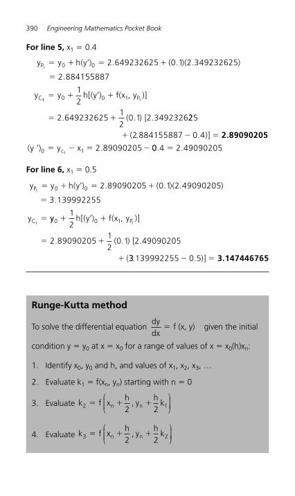
390 Engineering Mathematics Pocket Book
For line 5, x1 � 0.4
y y h(y ) ( )( )
y
P
C
1 0 0 2 649232625 0 1 2 349232625
2 884155887
� � � � �
�
. . .
.
11 10 0 112
2 64923262512
0 1 2 3492326
� � � �
� �
y h[(y ) f(x , y )]
( ) [
P
. . . 225
884155887 0 4
2 890902050 11
� � �
� � � � �
(2 )]
(y ) y xc
. .
.
2.89090205
00 4. � 2.49090205
For line 6, x1 � 0.5
y y h(y ) ( )( )
y
P
C
1
1
0 0 2 89090205 0 1 2 49090205
3 139992255
� � � � �
�
�
. . .
.
yy h[(y ) f(x , y )]
( ) [
(
P0 0 112
2 8909020512
0 1 2 49090205
1� � �
� �
�
. . .
33 )]. .139992255 0 5� � 3.147446765
Runge-Kutta method
To solve the differential equation dydx
f (x, y)� given the initial
condition y � y0 at x � x0 for a range of values of x � x0(h)xn:
1. Identify x0, y0 and h, and values of x1, x2, x3, …
2. Evaluate k1 � f(xn, yn) starting with n � 0
3. Evaluate k f xh
, yh
kn n2 12 2� � �
⎛⎝⎜⎜⎜
⎞⎠⎟⎟⎟⎟
4. Evaluate k f xh
, yh
kn n3 22 2� � �
⎛⎝⎜⎜⎜
⎞⎠⎟⎟⎟⎟
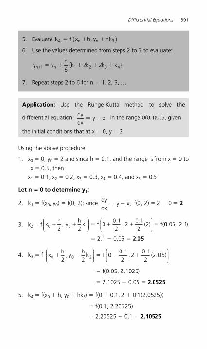
Differential Equations 391
Using the above procedure:
1. x0 � 0, y0 � 2 and since h � 0.1, and the range is from x � 0 to
x � 0.5, then
x1 � 0.1, x2 � 0.2, x3 � 0.3, x4 � 0.4, and x5 � 0.5
Let n � 0 to determine y1:
2. k1 � f(x0, y0) � f(0, 2); since dydx
y x,� � f(0, 2) � 2 � 0 � 2
3. k2 � f xh
, yh
k f , ( ) (0 0 12 20
0 12
20 12
2� � � � � �⎛⎝⎜⎜⎜
⎞⎠⎟⎟⎟⎟
⎛⎝⎜⎜⎜
⎞⎠⎟⎟⎟⎟
. .f 00.05, )2 1.
� 2.1 � 0.05 � 2.05
4. k3 � f xh
, yh
k f , ( )0 0 22 20
0 12
20 12
2 05� � � � �⎛⎝⎜⎜⎜
⎞⎠⎟⎟⎟⎟
⎛⎝⎜⎜⎜
⎞⎠⎟⎟⎟⎟
. ..
� f(0.05, 2.1025)
� 2.1025 � 0.05 � 2.0525
5. k4 � f(x0 � h, y0 � hk3) � f(0 � 0.1, 2 � 0.1(2.0525))
� f(0.1, 2.20525)
� 2.20525 � 0.1 � 2.10525
5. Evaluate k f x h, y hkn n4 3� � �( )
6. Use the values determined from steps 2 to 5 to evaluate:
y yh
{k k k k }n n� � � � � �1 1 2 3 462 2
7. Repeat steps 2 to 6 for n � 1, 2, 3, …
Application: Use the Runge-Kutta method to solve the
differential equation: dydx
y x� � in the range 0(0.1)0.5, given
the initial conditions that at x � 0, y � 2
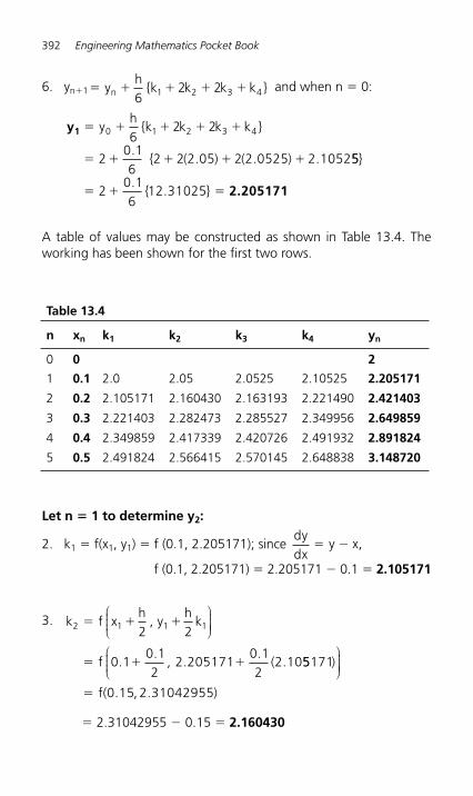
392 Engineering Mathematics Pocket Book
6. yn�1� � � � �yh
{k k k k }n 62 21 2 3 4 and when n � 0:
y1 � � � � �
� � � � �
yh
{k k k k }
{ ( ) ( )
0 1 2 3 462 2
20 16
2 2 2 05 2 2 0525 2 1052.
. . . 55
20 16
12 31025
}
{ }� � �.
. 2.205171
A table of values may be constructed as shown in Table 13.4. The working has been shown for the first two rows.
Table 13.4
n xn k1 k2 k3 k4 yn
0 0 2
1 0.1 2.0 2.05 2.0525 2.10525 2.205171
2 0.2 2.105171 2.160430 2.163193 2.221490 2.421403
3 0.3 2.221403 2.282473 2.285527 2.349956 2.649859
4 0.4 2.349859 2.417339 2.420726 2.491932 2.891824
5 0.5 2.491824 2.566415 2.570145 2.648838 3.148720
Let n � 1 to determine y2:
2. k1 � f(x1, y1) � f (0.1, 2.205171); since dydx
y x,� �
f (0.1, 2.205171) � 2.205171 � 0.1 � 2.105171
3. k f2 1 1 12 2
0 10 12
2 2051710 12
2 10
� � �
� � �
xh
, yh
k
f , (
⎛⎝⎜⎜⎜
⎞⎠⎟⎟⎟⎟
..
..
. 55171
0 15 2 31042955
)
f( )
⎛⎝⎜⎜⎜
⎞⎠⎟⎟⎟⎟
� . , .
� 2.31042955 � 0.15 � 2.160430
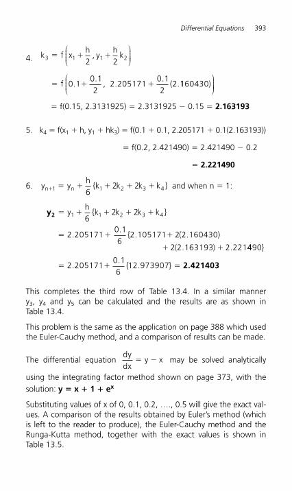
Differential Equations 393
4. k3 1 1 22 2
0 10 12
2 2051710 12
2
� � �
� � �
f xh
, yh
k
f , (
⎛⎝⎜⎜⎜
⎞⎠⎟⎟⎟⎟
..
..
.1160430)⎛⎝⎜⎜⎜
⎞⎠⎟⎟⎟⎟
� f(0.15, 2.3131925) � 2.3131925 � 0.15 � 2.163193
5. k4 � f(x1 � h, y1 � hk3) � f(0.1 � 0.1, 2.205171 � 0.1(2.163193))
� f(0.2, 2.421490) � 2.421490 � 0.2
� 2.221490
6. y yh
{k k k k }n 1 n� � � � � �6
2 21 2 3 4 and when n � 1:
y2 � � � � �
� � �
yh
{k k k k }
{ ( )
1 1 2 3 462 2
2 2051710 16
2 105171 2 2 160430..
. .
( )� �2 2 163193 2 221. . 4490
2 2051710 16
12 973907
}
{ }� � �..
. 2.421403
This completes the third row of Table 13.4. In a similar manner y3, y4 and y5 can be calculated and the results are as shown in Table 13.4.
This problem is the same as the application on page 388 which used the Euler-Cauchy method, and a comparison of results can be made.
The differential equation dydx
y x� � may be solved analytically
using the integrating factor method shown on page 373, with the solution: y � x � 1 � ex
Substituting values of x of 0, 0.1, 0.2, …., 0.5 will give the exact val-ues. A comparison of the results obtained by Euler’s method (which is left to the reader to produce), the Euler-Cauchy method and the Runga-Kutta method, together with the exact values is shown in Table 13.5.
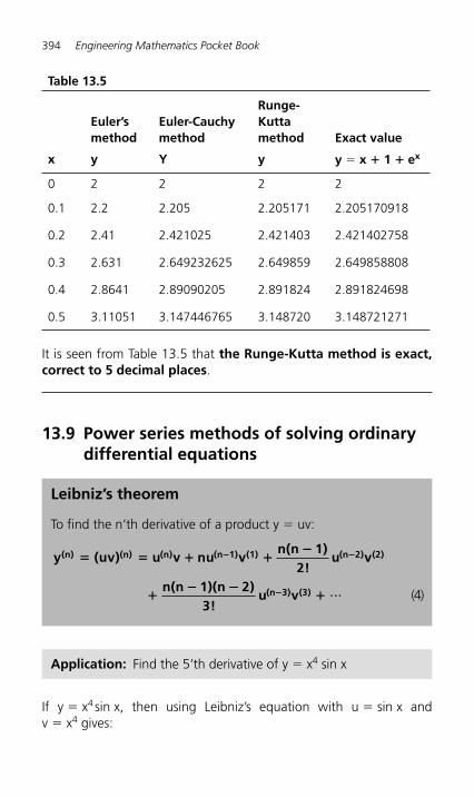
394 Engineering Mathematics Pocket Book
13.9 Power series methods of solving ordinary differential equations
Leibniz’s theorem
To find the n’th derivative of a product y � uv:
y (uv) u v nu vn(n 1)
2!u v
n(n 1)(n
(n) (n) (n) (n 1) (1) (n 2) (2)� � � ��
��
� �
����2)
3!u v(n 3) (3) ... (4)
Application: Find the 5’th derivative of y � x4 sin x
If y � x4 sin x, then using Leibniz’s equation with u � sin x and v � x4 gives:
Table 13.5
Euler’s method
Euler-Cauchy method
Runge-Kuttamethod Exact value
x y Y y y � x � 1 � ex
0 2 2 2 2
0.1 2.2 2.205 2.205171 2.205170918
0.2 2.41 2.421025 2.421403 2.421402758
0.3 2.631 2.649232625 2.649859 2.649858808
0.4 2.8641 2.89090205 2.891824 2.891824698
0.5 3.11051 3.147446765 3.148720 3.148721271
It is seen from Table 13.5 that the Runge-Kutta method is exact, correct to 5 decimal places.

Differential Equations 395
y xn
x n x(n )(n) � � � �
�sin sin
π π2
12
4⎛⎝⎜⎜⎜
⎞⎠⎟⎟⎟⎟
⎡
⎣⎢⎢
⎤
⎦⎥⎥
⎛⎝⎜⎜⎜
⎞⎠⎟⎟⎟⎟⎟
⎡
⎣⎢⎢
⎤
⎦⎥⎥
⎛⎝⎜⎜⎜
⎞⎠⎟⎟⎟⎟
⎡
⎣⎢⎢
⎤
⎦⎥⎥
4
12
22
12
3
2
x
n(n )!
x(n )
x��
��
�
sinπ
nn(n )(n )!
x(n )
x
n(n )(n
� ��
�
�� �
1 23
32
24
1
sinπ⎛
⎝⎜⎜⎜
⎞⎠⎟⎟⎟⎟
⎡
⎣⎢⎢
⎤
⎦⎥⎥
22 34
42
)(n )!
x(n )
24�
��
sinπ⎛
⎝⎜⎜⎜
⎞⎠⎟⎟⎟⎟
⎡
⎣⎢⎢
⎤
⎦⎥⎥
and
y x x x (x )( )( )
( x ) x( )5 4 3 252
20 25 4
212� � � � �sin sin sin
ππ
⎛⎝⎜⎜⎜
⎞⎠⎟⎟⎟⎟ ��
32π⎛
⎝⎜⎜⎜
⎞⎠⎟⎟⎟⎟
� � �( )( )( )
( )( )( x) (x )
( )( )( )( )( )( )( )
( )5 4 3
3 224
5 4 3 24 3 2
24sin sinπ xx �π2
⎛⎝⎜⎜⎜
⎞⎠⎟⎟⎟⎟
Since sin sin cosx x x,� �52 2π
≡ π
≡⎛⎝⎜⎜⎜
⎞⎠⎟⎟⎟⎟
⎛⎝⎜⎜⎜
⎞⎠⎟⎟⎟⎟ sin(x � 2π)� sin x,
sin cosx x,� �32π
≡⎛⎝⎜⎜⎜
⎞⎠⎟⎟⎟⎟
and sin (x � π) � �sin x,
then y(5) � x4 cos x � 20x3 sin x � 120x2 (�cos x)
� 240x (�sin x) � 120 cos xi.e. y(5) � (x4 � 120x2 � 120) cos x �(20x3 � 240x) sin x
Leibniz-Maclaurin method
(i) Differentiate the given equation n times, using the Leibniz theorem of equation (4),
(ii) rearrange the result to obtain the recurrence relation at x � 0,
(iii) determine the values of the derivatives at x � 0, i.e. find (y)0and (y�)0,
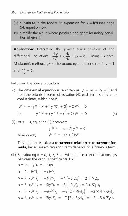
396 Engineering Mathematics Pocket Book
Following the above procedure:
(i) The differential equation is rewritten as: y� � xy� � 2y � 0 and from the Leibniz theorem of equation (4), each term is differenti-ated n times, which gives:
y y (x) n y ( ) y(n ) (n ) (n) (n)� �� � � � �2 1 1 0 2 0{ }i.e. y x y (n ) y(n ) (n ) (n)� �� � � �2 1 2 0 (5)
(ii) At x � 0, equation (5) becomes:
y (n ) y(n ) (n)� � �2 2 0+
from which, y (n ) y(n ) (n)� � � �2 2
This equation is called a recurrence relation or recurrence for-mula, because each recurring term depends on a previous term.
(iii) Substituting n � 0, 1, 2, 3, … will produce a set of relationships between the various coefficients. For
n � 0, (y ) (y)� � �0 02
n � 1, (y ) (y )� � � �0 03
n � 2, (y ) (y ) (y) (y)( )40 0 0 04 4 2 2 4� � � � � � � �{ }
n � 3, (y ) (y ) (y ) (y )( )50 0 0 05 5 3 3 5� � � � � � � � � �{ }
n � 4, (y ) (y ) (y) (y)( ) ( )60
40 0 06 6 2 4 2 4 6� � � � � � � � �{ }
n � 5, (y ) (y ) (y ) (y )( ) ( )70
50 0 07 7 3 5 3 5 7� � � � � � � � � � �{ }
Application: Determine the power series solution of the
differential equation: d ydx
xdydx
y2
22 0� � � using Leibniz-
Maclaurin’s method, given the boundary conditions x � 0, y � 1
and dydx
� 2
(iv) substitute in the Maclaurin expansion for y � f(x) (see page 54, equation (5)),
(v) simplify the result where possible and apply boundary condi-tion (if given).
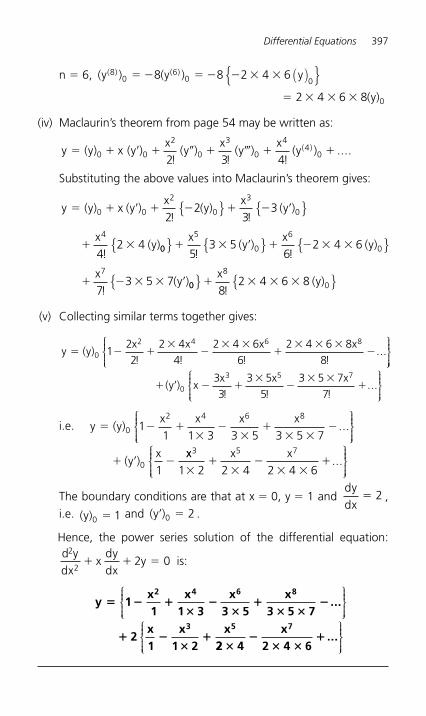
Differential Equations 397
n � 6, (y ) (y )( ) ( )80
60 0
8 8 2 4 6� � � � � � �
y( ){ } � � � �2 4 6 8 0(y)
(iv) Maclaurin’s theorem from page 54 may be written as:
y (y) x (y )x!
(y )x!
(y )x
!(y ) ....0
( )� � � � � � � � �0
2
0
3
0
44
02 3 4
Substituting the above values into Maclaurin’s theorem gives:
y (y) x (y )x!
(y)x!
(y )
x!
(y)
� � � � � � � �
� �
0 0
2
0
3
0
4
22
33
42 4
{ } { }
00
5
0
6
0
7
53 5
62 4 6
73 5 7
{ } { } { }� � � � � � �
� � � � �
x!
(y )x!
(y)
x!
(y )008
082 4 6 8{ } { }� � � �
x!
(y)
(v) Collecting similar terms together gives:
y (y)x!
x!
x!
x!
...� � ��
�� �
�� � �
�0
2 4 6 81
22
2 44
2 4 66
2 4 6 88
⎧⎨⎪⎪⎩⎪⎪
⎫⎬⎪⎪⎭⎭⎪⎪
⎧⎨⎪⎪⎩⎪⎪
⎫⎬⎪⎪⎭⎪⎪
� � � ��
�� �
�(y ) xx!
x!
x!
...0
3 5 733
3 55
3 5 77
i.e. y (y)x x x x
...
(y )x
� � ��
��
�� �
�
� � �
0
2 4 6 8
0
11 1 3 3 5 3 5 7
1
⎧⎨⎪⎪⎩⎪⎪
⎫⎬⎪⎪⎭⎪⎪
xx x4
x...
3 5 7
1 2 2 2 4 6��
��
� ��
⎧⎨⎪⎪⎩⎪⎪
⎫⎬⎪⎪⎭⎪⎪
The boundary conditions are that at x � 0, y � 1 and dydx
2� ,i.e. (y)0 1� and (y )� �0 2 .
Hence, the power series solution of the differential equation:d ydx
xdydx
y2
22 0� � � is:
y 1x1
x1 3
x3 5
x3 5 7
...
2x1
x1 2
x
2 4 6 8
3 5
� � ��
��
�� �
�
� ��
�
⎧⎨⎪⎪⎩⎪⎪
⎫⎬⎪⎪⎭⎪⎪
22 4x
2 4 6...
7
��
� ��
⎧⎨⎪⎪⎩⎪⎪
⎫⎬⎪⎪⎭⎪⎪
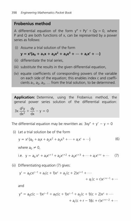
398 Engineering Mathematics Pocket Book
The differential equation may be rewritten as: 3xy� � y� � y � 0
(i) Let a trial solution be of the form
y x {a a x a x a x ... a x ...}cr
r� � � � � � �0 1 22
33 (6)
where a0 � 0,
i.e. y a x a x a x a x ... a x ...c c c cr
c r� � � � � � �� � � �0 1
12
23
3 (7)
(ii) Differentiating equation (7) gives:
y a cx a (c )x a (c )x ....
a (c r)x ...0
c c c
rc r
� � � � � � �
� � �
� �
� �
11 2
1
1
1 2
and
y a c(c )x a c(c )x a (c )(c )x ....
a (c r )
c c c
r
� � � � � � � � �
� � �
� �0
21
121 1 1 2
1 ((c r)x ...c r� �� �2
Frobenius method
A differential equation of the form y″ � Py� � Qy � 0, where P and Q are both functions of x, can be represented by a power series as follows:
(i) Assume a trial solution of the form
y � xc{a0 � a1x � a2x2 � a3x3 � … � arxr � …}
(ii) differentiate the trial series,
(iii) substitute the results in the given differential equation,
(iv) equate coefficients of corresponding powers of the variable on each side of the equation; this enables index c and coeffi-cients a1, a2, a3, … from the trial solution, to be determined.
Application: Determine, using the Frobenius method, the general power series solution of the differential equation:
3xd ydx
dydx
y 02
2� � �
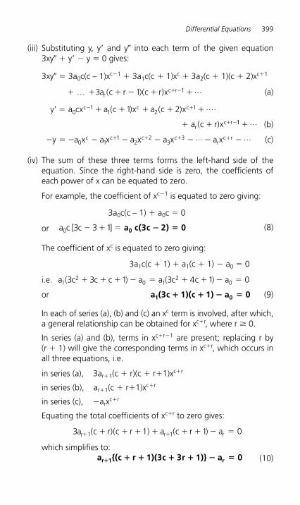
Differential Equations 399
(iii) Substituting y, y� and y� into each term of the given equation 3xy� � y� � y � 0 gives:
3xy� � 3a0c(c – 1)xc�1 � 3a1c(c � 1)xc � 3a2(c � 1)(c � 2)xc�1
� … � � � � �� �3 1 1a (c r )(c r)x ...r
c r (a)
y a cx a (c )x a (c )x ....
a (c r)x
c c c
rc r
� � � � � � �
� �
� �
� �
01
1 211 2
11 � ... (b)
� � � � � � � � �� � �y a x a x a x a x ... a x ...c c c cr
c r0 1
12
23
3 + (c)
(iv) The sum of these three terms forms the left-hand side of the equation. Since the right-hand side is zero, the coefficients of each power of x can be equated to zero.
For example, the coefficient of xc�1 is equated to zero giving:
3a0c(c – 1) � a0c � 0
or a c [ c ]0 3 3 1� � � a c(3c 2) 00 � � (8)
The coefficient of xc is equated to zero giving:
3a1c(c � 1) � a1(c � 1) � a0 � 0
i.e. a ( c c c ) a a ( c c ) a12
0 12
03 3 1 3 4 1 0� � � � � � � � �
or a (3c 1)(c 1) a 01 0� � � � (9)
In each of series (a), (b) and (c) an xc term is involved, after which, a general relationship can be obtained for xc�r, where r � 0.
In series (a) and (b), terms in xc�r�1 are present; replacing r by (r � 1) will give the corresponding terms in xc�r, which occurs in all three equations, i.e.
in series (a), 3ar�1(c � r)(c � r�1)xc�r
in series (b), ar�1(c � r�1)xc�r
in series (c), �arxc�r
Equating the total coefficients of xc�r to zero gives:
3 1 01 1a (c r)(c r 1) a (c r ) ar r r� �� � � � � � � �
which simplifies to:a {(c r 1)(3c 3r 1)} a 0r 1 r� � � � � � � (10)
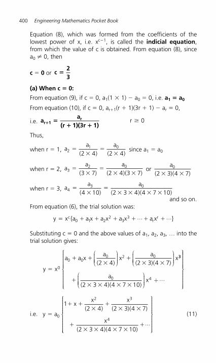
400 Engineering Mathematics Pocket Book
Equation (8), which was formed from the coefficients of the lowest power of x, i.e. xc�1, is called the indicial equation,from which the value of c is obtained. From equation (8), since a0 � 0, then
c � 0 or c23
�
(a) When c � 0:
From equation (9), if c � 0, a1(1 � 1) � a0 � 0, i.e. a1 � a0
From equation (10), if c � 0, ar�1(r � 1)(3r � 1) � ar � 0,
i.e. aa
(r 1)(3r 1)r 1r
� �� �
r 0�
Thus,
when r � 1, aa
( )a
( )21 0
2 4 2 4�
��
� since a1 � a0
when r � 2, aa
( )a
( )( )32 0
3 7 2 4 3 7�
��
� � or
a( )( )
0
2 3 4 7� �
when r � 3, aa
( )a
( )( )43 0
4 10 2 3 4 4 7 10�
��
� � � �and so on.
From equation (6), the trial solution was:
y x {a a x a x a x ... a x ...}cr� � � � � � �0 1 2
23
3 r
Substituting c � 0 and the above values of a1, a2, a3, … into the trial solution gives:
y x
a a xa
( )x
a( )( )
x
�
� ��
�� �
0
0 00 2 0
2 4 2 3 4 7
⎛
⎝⎜⎜⎜⎜
⎞
⎠⎟⎟⎟⎟
⎛
⎝⎜⎜⎜⎜
⎞
⎠⎟⎟⎟⎟
33
0 4
2 3 4 4 7 10 �
� � � �
a( )( )
x ...⎛
⎝⎜⎜⎜⎜
⎞
⎠⎟⎟⎟⎟ +
⎧
⎨
⎪⎪⎪⎪⎪⎪⎪
⎩
⎪⎪⎪⎪⎪⎪⎪
⎫
⎬
⎪⎪⎪⎪⎪⎪⎪⎪
⎭
⎪⎪⎪⎪⎪⎪⎪
i.e. y a
xx
( )x
( )( )
x( )( )
...
�
� ��
�� �
�� � � �
�
0
2 3
4
12 4 2 3 4 7
2 3 4 4 7 10
⎧
⎨
⎪⎪⎪⎪⎪⎪
⎩⎩
⎪⎪⎪⎪⎪⎪
⎫
⎬
⎪⎪⎪⎪⎪⎪
⎭
⎪⎪⎪⎪⎪⎪
(11)
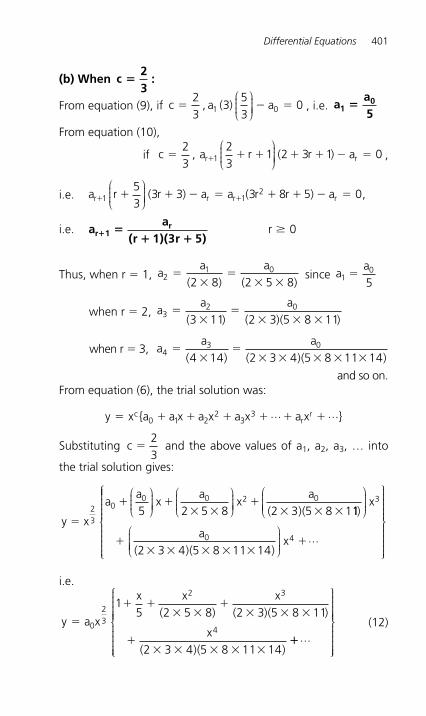
Differential Equations 401
(b) When c23
� :
From equation (9), if c , a ( ) a� � �23
353
01 0⎛⎝⎜⎜⎜
⎞⎠⎟⎟⎟⎟ , i.e. a
a510�
From equation (10),
if c , a r ( r ) ar r� � � � � � ��
23
23
1 2 3 1 01⎛⎝⎜⎜⎜
⎞⎠⎟⎟⎟⎟ ,
i.e. a r ( r ) a a ( r r ) a 0,r r r r� �� � � � � � � �1 125
33 3 3 8 5
⎛⎝⎜⎜⎜
⎞⎠⎟⎟⎟⎟
i.e. aa
(r 1)(3r 5)r 1r
� �� �
r 0�
Thus, when r � 1, aa
( )a
( )21 0
2 8 2 5 8�
��
� � since a
a1
0
5�
when r � 2, aa
( )a
( )( )32 0
3 11 2 3 5 8 11�
��
� � �
when r � 3, aa
( )a
( )( )43 0
4 14 2 3 4 5 8 11 14�
��
� � � � �
and so on.From equation (6), the trial solution was:
y x {a a x a x a x ... a x ...}rr� � � � � � �c
0 1 22
33
Substituting c �23
and the above values of a1, a2, a3, … into
the trial solution gives:
y x
aa
xa
xa
( 3)(�
� �� �
�� � �2
3
00 0 2 0
5 2 5 8 2 5 8 1
⎛⎝⎜⎜⎜
⎞⎠⎟⎟⎟⎟
⎛⎝⎜⎜⎜
⎞⎠⎟⎟⎟⎟ 11
2 3 4 5 8 11 14
3
0 4
)x
a( )( )
x ...
⎛
⎝⎜⎜⎜⎜
⎞
⎠⎟⎟⎟⎟
⎛
⎝⎜⎜⎜⎜
⎞
⎠⎟⎟⎟⎟
⎧
⎨
�� � � � �
�
⎪⎪⎪⎪⎪⎪⎪
⎩
⎪⎪⎪⎪⎪⎪
⎫
⎬
⎪⎪⎪⎪⎪⎪
⎭
⎪⎪⎪⎪⎪⎪
i.e.
y a x
x x( )
x( )( )
x( )( )
�
� �� �
�� � �
�� � � � �
0
23
2 3
4
15 2 5 8 2 3 5 8 11
2 3 4 5 8 11 14��...
⎧
⎨
⎪⎪⎪⎪⎪⎪
⎩
⎪⎪⎪⎪⎪⎪
⎫
⎬
⎪⎪⎪⎪⎪⎪
⎭
⎪⎪⎪⎪⎪⎪
(12)
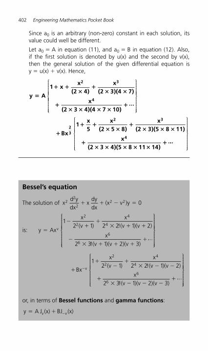
402 Engineering Mathematics Pocket Book
Since a0 is an arbitrary (non-zero) constant in each solution, its value could well be different.
Let a0 � A in equation (11), and a0 � B in equation (12). Also, if the first solution is denoted by u(x) and the second by v(x), then the general solution of the given differential equation is y � u(x) � v(x). Hence,
y A
1 xx
(2 4)x
(2 3)(4 7)
x(2 3 4)(4 7 10)
2 3
4�
� ��
�� �
�� � � �
� ...
⎧
⎨
⎪⎪⎪⎪⎪⎪
⎩
⎪⎪⎪⎪⎪⎪⎪
⎫
⎬
⎪⎪⎪⎪⎪⎪
⎭
⎪⎪⎪⎪⎪⎪
�
� �� �
�� � �
�� � � � �
�
Bx
1x5
x(2 5 8)
x(2 3)(5 8 11)
x(2 3 4)(5 8 11 14)
23
2 3
4....
⎧
⎨
⎪⎪⎪⎪⎪⎪
⎩
⎪⎪⎪⎪⎪⎪
⎫
⎬
⎪⎪⎪⎪⎪⎪
⎭
⎪⎪⎪⎪⎪⎪
Bessel’s equation
The solution of xd ydx
xdydx
(x v )y22
22 2 0� � � �
is: y Ax
x(v )
x!(v )(v )
x!(v )(v )(v )
v�
��
�� � �
�� � � �
�
12 1 2 2 1 2
2 3 1 2 3
2
2
4
4
6
6....
⎧
⎨
⎪⎪⎪⎪⎪⎪
⎩
⎪⎪⎪⎪⎪⎪
⎫
⎬
⎪⎪⎪⎪⎪⎪
⎭
⎪⎪⎪⎪⎪⎪
�
��
�� � �
�� � � �
�
�Bx
x(v )
x!(v )(v )
x!(v )(v )(v )
v
12 1 2 2 1 2
2 3 1 2 3
2
2
4
4
6
6....
⎧
⎨
⎪⎪⎪⎪⎪⎪
⎩
⎪⎪⎪⎪⎪⎪
⎫
⎬
⎪⎪⎪⎪⎪⎪
⎭
⎪⎪⎪⎪⎪⎪
or, in terms of Bessel functions and gamma functions:
y A J (x) BJ (x)v v� � �
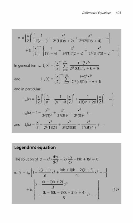
Differential Equations 403
��
��
��
�Ax
(v )x
( !) (vx
( !) (v ).
v
21
1 2 1 2 2 2 4
2
2
4
4
⎛⎝⎜⎜⎜
⎞⎠⎟⎟⎟⎟ Γ Γ Γ)
...
Bx
( v)x
( !)
v
⎧⎨⎪⎪⎩⎪⎪
⎫⎬⎪⎪⎭⎪⎪
⎛⎝⎜⎜⎜
⎞⎠⎟⎟⎟⎟ �
��
�
21
1 2 1
2
2Γ Γ(( v)x
( !) ( v)...
2 2 2 3
4
4��
��
Γ
⎧⎨⎪⎪⎩⎪⎪
⎫⎬⎪⎪⎭⎪⎪
In general terms: J (x)x ( ) x
(k!) (v k )v
v k k
kk
��
� ��21
2 1
2
20
⎛⎝⎜⎜⎜
⎞⎠⎟⎟⎟⎟ ∑ Γ
�
and J (x)x ( ) x
(k!) (k v )v
v k k
kk
�
�
�
��
� �21
2 1
2
20
⎛⎝⎜⎜⎜
⎞⎠⎟⎟⎟⎟ ∑ Γ
�
and in particular:
J (x)x
n! (n )!x
( !)(n )!x
n
n
� ��
��2
1 11 2
12 2
2⎛⎝⎜⎜⎜
⎞⎠⎟⎟⎟⎟
⎛⎝⎜⎜⎜
⎞⎠⎟⎟⎟⎟ 22
4⎛⎝⎜⎜⎜
⎞⎠⎟⎟⎟⎟
⎧⎨⎪⎪⎪
⎩⎪⎪⎪
⎫⎬⎪⎪⎪
⎭⎪⎪⎪
� ...
J (x)x( !)
x( )
x( !)
...0
2
2 2
4
4 2
6
6 21
2 1 2 2 2 3� � �
!− +
and J (x)x x
( !)( !)x
( !)( !)x
( !)( !)...
1
3
3
5
5
7
72 2 1 2 2 2 3 2 3 4� � � � +
Legendre’s equation
The solution of ( x )d ydx
xdydx
k(k )y1 2 1 022
2� � � � �
is: y ak(k )
!x
k(k )(k )(k )!
x ...� ��
�� � �
�02 41
12
1 2 34
⎧⎨⎪⎪⎩⎪⎪
⎫⎬⎪⎪⎭⎪⎪
�
�� �
�� � � �
�
ax
(k )(k )!
x
(k )(k )(k )(k )!
x ...1
3
5
1 231 3 2 4
5
⎧
⎨
⎪⎪⎪⎪⎪
⎩
⎪⎪⎪⎪⎪⎪
⎫
⎬
⎪⎪⎪⎪⎪
⎭
⎪⎪⎪⎪⎪
(13)
404 Engineering Mathematics Pocket Book
Legendre’s polynomials
Rodrigue’s formula
P (x)1
2 n!d (x 1)
dxn n
n 2 n
n�
�
Application: Determine the Legendre polynomial P3(x) using Rodrigue’s formula
In Rodrigue’s formula, P (x)n!
d (x )n n
n n�
�12
12
dxn and when n � 3,
P (x)!
d (x )dx ( )
d (x )(x x )dx
( )(
3 3
3 2 3
3 3
3 2 4 2
3
12 3
1 12 6
1 2 1
18 6
��
�� � �
�))
d (x x x )dx
3 6 4 2
3
3 3 1� � �
d(x x x )dx
x x x6 4 2
5 33 3 16 12 6
� � �� � �
Application: Determine the Legendre polynomial P 3 (x)
Since in P3(x), n � k � 3, then from the second part of equation (13), i.e. the odd powers of x:
y a x(k )(k )
!x
(k )(k )(k )(k )!
x ...� �� �
�� � � �
�13 51 2
31 3 2 4
5
⎧⎨⎪⎪⎩⎪⎪
⎫⎬⎪⎪⎪⎭⎪⎪
i.e. y a x( )( )
!x
( )( )( )( )!
x a x x� � � � � �13 5
132 5
32 0 5 7
553
0⎧⎨⎪⎪⎩⎪⎪
⎫⎬⎪⎪⎭⎪⎪
⎧⎧⎨⎪⎪⎩⎪⎪
⎫⎬⎪⎪⎭⎪⎪
a1 is chosen to make y � 1 when x � 1.
i.e. 1 153
231 1� � � �a a
⎧⎨⎪⎪⎩⎪⎪
⎫⎬⎪⎪⎭⎪⎪
⎛⎝⎜⎜⎜
⎞⎠⎟⎟⎟⎟ from which, a1
32
� �
Hence, P (x) x x333
253
� � �⎛⎝⎜⎜⎜
⎞⎠⎟⎟⎟⎟ or P (x)
12
(5x 3x)33� �
Differential Equations 405
d( x x x)dx
x x6 12 6
30 36 65 3
4 2� �� � �
andd( x x )
dxx x
30 36 6120 72
4 23� �
� �
Hence, P (x)( )( )
d (x x x )dx
( )( )( x x) ( x
3
3 6 4 2
3
3
18 6
3 3 1
18 6
120 7218
20
�� � �
� � � 33 12� x)
i.e. P (x)12
(5x 3x)33� � the same as in the previous
application.
13.10 Solution of partial differential equations
By direct partial integration
Application: Solve the differential equation ∂∂
2
226 2 1
ux
x ( y )� �
given the boundary conditions that at x � 0, ∂∂
ux
y� sin 2 and u � cos y
Since∂∂
2
226 1
ux
x (2y )� � then integrating partially with respect to x
gives:
∂∂
ux
x ( y ) dx ( y ) x dx ( y )x
f(y)
x ( y ) f
� � � � � � �
� � �
6 2 1 2 1 6 2 163
2 2 1
2 23
3
∫ ∫((y)
where f(y) is an arbitrary function.
From the boundary conditions, when x � 0, ∂∂
ux
y� sin 2
Hence, sin 2 2 0 2 13y ( ) ( y ) f(y)� � � from which, f(y) y� sin 2
406 Engineering Mathematics Pocket Book
Now∂∂
ux
x ( y ) y� � �2 2 1 23 sin
Integrating partially with respect to x gives:
u [ x ( y ) y] dxx
( y ) x( y) F(y)� � � � � � �2 2 1 224
2 1 234
sin sin∫From the boundary conditions, when x � 0, u � cos y, hence
cos siny � � � �( )
( y ) ( ) y F(y)02
2 1 0 24
from which, F(y) � cos y
Hence, the solution of ∂∂
2
226 2 1
ux
x ( y )� � for the given boundaryconditions is:
ux2
(2y 1) x sin y cos y4
� � � �
The wave equation
The wave equation is given by: ∂∂
∂∂
2
2 2
2
2
ux
1c
ut
�
where cT2 ��
, with T being the tension in a string and ρ being
the mass /unit length of the string.
Summary of solution of the wave equation
1. Identify clearly the initial and boundary conditions.
2. Assume a solution of the form u � XT and express the equa-tions in terms of X and T and their derivatives.
3. Separate the variables by transposing the equation and equate each side to a constant, say, μ; two separate equations are obtained, one in x and the other in t.
4. Let μ � �p2 to give an oscillatory solution.
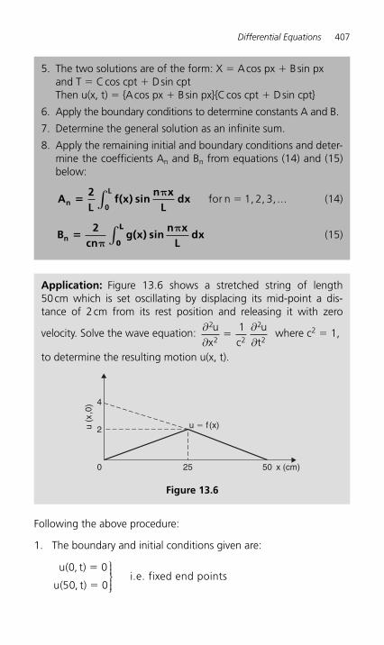
Differential Equations 407
5. The two solutions are of the form: X � A cos px � B sin px and T � C cos cpt � D sin cpt Then u(x, t) � {A cos px � B sin px}{C cos cpt � D sin cpt}
6. Apply the boundary conditions to determine constants A and B.
7. Determine the general solution as an infinite sum.
8. Apply the remaining initial and boundary conditions and deter-mine the coefficients An and Bn from equations (14) and (15) below:
A2L
f(x) sinn x
Ldxn
0
L�
π∫ for n 1, 2, 3, ...� (14)
B2
cng(x) sin
n xL
dxn �π
π0
L
∫ (15)
Application: Figure 13.6 shows a stretched string of length 50 cm which is set oscillating by displacing its mid-point a dis-tance of 2 cm from its rest position and releasing it with zero
velocity. Solve the wave equation: ∂∂
∂∂
2
2 2
2
2
1ux c
ut
� where c2 � 1,
to determine the resulting motion u(x, t).
250
2
4
50 x (cm)
u � f (x)u (x
,0)
Figure 13.6
Following the above procedure:
1. The boundary and initial conditions given are:
u( , t)
u( , t)i.e. fixed end points
0 0
50 0
�
�
⎫⎬⎪⎪
⎭⎪⎪
408 Engineering Mathematics Pocket Book
u(x, ) x 0 0 25� � �f(x)2
25x�
� � � � � �2
254 50x x
100 2x25�
25
(Note: y � mx � c is a straight line graph, so the gradient, m,between 0 and 25 is 2/25 and the y-axis intercept is zero, thus
y f(x) x� � �2
250; between 25 and 50, the gradient � �2/25
and the y-axis intercept is at 4, thus f(x) x� � �2
254 ).
∂∂ut
i.e. zero initial velocityt
⎡
⎣⎢⎢
⎤
⎦⎥⎥
�
�0
0
2. Assuming a solution u � XT, where X is a function of x only, and T is a function of t only,
then ∂∂
ux
X T� � and ∂∂
2
2
ux
X T� � and ∂∂
uy
XT� � and
∂∂
2
2
uy
XT� �
Substituting into the partial differential equation,
∂∂
∂∂
2
2 2
2
2
1ux c
ut
�
gives: X Tc
XT� ��12 i.e. X �T � XT� since c2 � 1
3. Separating the variables gives: XX
TT
��
�
Let constant, � ��
��X
XTT
then � ��X
X and � �
�TT
from which, X� � μX � 0 and T� � μ T � 0
Differential Equations 409
4. Letting μ � �p2 to give an oscillatory solution gives
X� � p2X � 0 and T � � p2 T � 0
The auxiliary equation for each is: m2 � p2 � 0 from which,
m p jp� � � 2
5. Solving each equation gives: X � A cos px � B sin px and T � C cos pt � D sin pt
Thus, u(x, t) � {A cos px � B sin px} {C cos pt � D sin pt}
6. Applying the boundary conditions to determine constants A and B gives:
(i) u(0, t) � 0, hence 0 � A{C cos pt � D sin pt} from which we conclude that A � 0
Therefore, u(x, t) B px {C pt D pt}� �sin cos sin (a)
(ii) u(50, t) � 0, hence 0 � B sin 50p{C cos pt � D sin pt}
B � 0 hence sin 50p � 0 from which, 50p � n�
and pn
��
50
7. Substituting in equation (a) gives:
u(x, t) Bn x
Cn t
Dn t
�� �
��
sin cos sin50 50 50
⎧⎨⎪⎪⎩⎪⎪
⎫⎬⎪⎪⎭⎪⎪
or, more generally,
u (x, t)n x
An t
Bn t
n n nn
�� �
��
�
�
sin cos sin50 50 501
⎧⎨⎪⎪⎩⎪⎪
⎫⎬⎪⎪⎭⎪⎪
∑ (b)
where An � BC and Bn � BD
8. From equation (14),
AL
f(x)n x
Ldxn
L�
�20
sin∫
��
�� �2
502
25 50100 2
25 50x
n xdx
x n xd
⎛⎝⎜⎜⎜
⎞⎠⎟⎟⎟⎟
⎛⎝⎜⎜⎜
⎞⎠⎟⎟⎟⎟sin sin xx
25
50
0
25
∫∫⎡
⎣⎢⎢
⎤
⎦⎥⎥
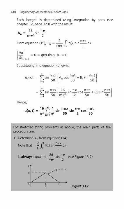
410 Engineering Mathematics Pocket Book
Each integral is determined using integration by parts (see chapter 12, page 323) with the result:
An ��
�1622 2n
nsin
From equation (15), Bcn
g(x)n x
Ldxn
L�
�
�20
sin∫
∂∂ut
g(x) thus, Bt
n⎡
⎣⎢⎢
⎤
⎦⎥⎥
�
� � �0
0 0
Substituting into equation (b) gives:
u (x,t)
n xA
n tB
n tn n n
n
�� �
��
�
�
sin cos sin50 50 501
⎧⎨⎪⎪⎩⎪⎪
⎫⎬⎪⎪⎭⎪⎪
∑
�
�
�
� ��
�
�
sin sin cos sinn x
nn n t
( )n t
n 5016
2 500
502 21
⎧⎨⎪⎪⎩⎪⎪
⎫⎬⎪⎪⎭⎪⎪
��
∑
Hence,
u(x, t)16 1
nsin
n x50
sinn2
cosn t502 2
n 1
��
� � �
�
∞
∑
For stretched string problems as above, the main parts of the procedure are:
1. Determine An from equation (14).
Note that2
0Lf(x)
n xL
dxL
sin�
∫
is always equal to 822 2
dn
n�
�sin (see Figure 13.7)
y
y � f (x)d
LL2
0 Figure 13.7
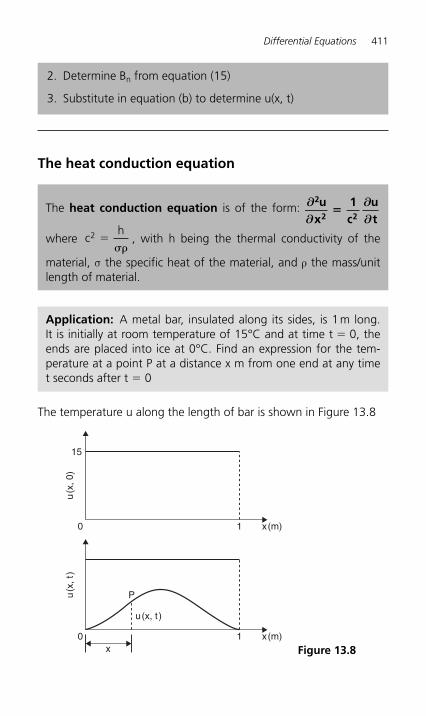
Differential Equations 411
The heat conduction equation
2. Determine Bn from equation (15)
3. Substitute in equation (b) to determine u(x, t)
The heat conduction equation is of the form: ∂∂
∂∂
2
2 2
ux
1c
ut
�
where ch2 �
��, with h being the thermal conductivity of the
material, σ the specific heat of the material, and ρ the mass/unit length of material.
Application: A metal bar, insulated along its sides, is 1 m long. It is initially at room temperature of 15°C and at time t � 0, the ends are placed into ice at 0°C. Find an expression for the tem-perature at a point P at a distance x m from one end at any time t seconds after t � 0
The temperature u along the length of bar is shown in Figure 13.8
0 1 x(m)
u(x
, 0)
15
0 1 x(m)
u(x
, t)
u (x, t )
x
P
Figure 13.8
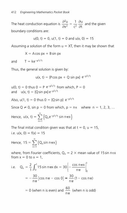
412 Engineering Mathematics Pocket Book
The heat conduction equation is ∂∂
∂∂
2
2 2
1ux c
ut
� and the given
boundary conditions are:
u(0, t) � 0, u(1, t) � 0 and u(x, 0) � 15
Assuming a solution of the form u � XT, then it may be shown that
X � A cos px � B sin px
and T ke p c t� � 2 2
Thus, the general solution is given by:
u(x, t) � {P cos px � Q sin px} e p c t� 2 2
u(0, t) � 0 thus 0 � P e p c t� 2 2 from which, P � 0
and u(x, t) � {Q sin px} e p c t� 2 2
Also, u(1, t) � 0 thus 0 � {Q sin p} e p c t� 2 2
Since Q � 0, sin p � 0 from which, p � nπ where n � 1, 2, 3, …
Hence, u(x, t) Q e n xnp c t
n
� ��
�
�2 2
1
sin{ }∑
The final initial condition given was that at t � 0, u � 15,
i.e. u(x, 0) � f(x) � 15
Hence, 151
� ��
�
Q n xnn
sin{ }∑
where, from Fourier coefficients, Qn � 2 � mean value of 15 sin nπxfrom x � 0 to x � 1,
i.e. Q n x dxn x
n
nn
n � � � ��
�
� ��
� �
21
15 30
300
0
1
0
1
sincos
cos cos
∫⎡
⎣⎢⎢
⎤
⎦⎥⎥
[ ] ���
� �30
1n
( n )cos
� 0 (when n is even) and 60n�
(when n is odd)
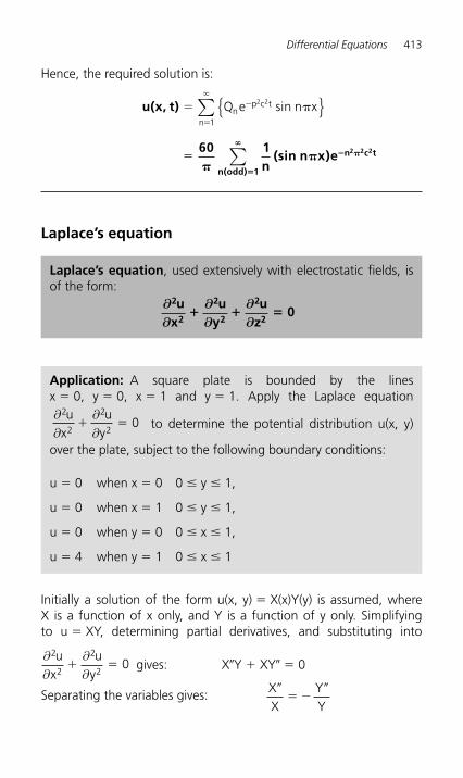
Differential Equations 413
Hence, the required solution is:
u(x, t) � ��
�
�
Q e n xnp c t
n
2 2
1
sin{ }∑
�
60 1n
(sin n x)en(odd) 1
n c t2 2 2
��
�
�� �∑
Laplace’s equation
Laplace’s equation, used extensively with electrostatic fields, is of the form:
∂∂
∂∂
∂∂
2
2
2
2
2
2
ux
uy
uz
0� � �
Application: A square plate is bounded by the lines x � 0, y � 0, x � 1 and y � 1. Apply the Laplace equation∂∂
∂∂
2
2
2
20
ux
uy
� � to determine the potential distribution u(x, y)
over the plate, subject to the following boundary conditions:
u � 0 when x � 0 0 � y � 1,
u � 0 when x � 1 0 � y � 1,
u � 0 when y � 0 0 � x � 1,
u � 4 when y � 1 0 � x � 1
Initially a solution of the form u(x, y) � X(x)Y(y) is assumed, where X is a function of x only, and Y is a function of y only. Simplifying to u � XY, determining partial derivatives, and substituting into
∂∂
∂∂
2
2
2
20
ux
uy
� � gives: X�Y � XY� � 0
Separating the variables gives: XX
YY
�� �
�
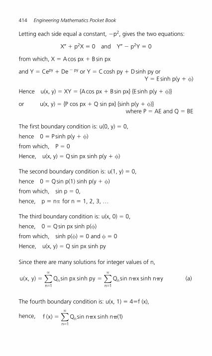
414 Engineering Mathematics Pocket Book
Letting each side equal a constant, �p2, gives the two equations:
X� � p2X � 0 and Y� � p2Y � 0
from which, X � A cos px � B sin px
and Y � Cepy � De � py or Y � C cosh py � D sinh py or Y � E sinh p(y � φ)
Hence u(x, y) � XY � {A cos px � B sin px} {E sinh p(y � φ)}
or u(x, y) � {P cos px � Q sin px} {sinh p(y � φ)} where P � AE and Q � BE
The first boundary condition is: u(0, y) � 0,
hence 0 � P sinh p(y � φ)
from which, P � 0
Hence, u(x, y) � Q sin px sinh p(y � φ)
The second boundary condition is: u(1, y) � 0,
hence 0 � Q sin p(1) sinh p(y � φ)
from which, sin p � 0,
hence, p � nπ for n � 1, 2, 3, …
The third boundary condition is: u(x, 0) � 0,
hence, 0 � Q sin px sinh p(φ)
from which, sinh p(φ) � 0 and φ � 0
Hence, u(x, y) � Q sin px sinh py
Since there are many solutions for integer values of n,
u(x, y) Q px py Q n x n ynn
nn
� � � ��
�
�
�
sin sinh sin sinh1 1
∑ ∑ (a)
The fourth boundary condition is: u(x, 1) � 4�f (x),
hence, f (x) Q n x n ( )nn
� � ��
�
sin sinh 11
∑
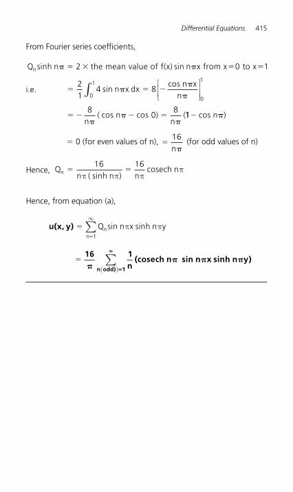
Differential Equations 415
From Fourier series coefficients,
Q n the mean value of f(x) x from x to xnsinh sin� � � � � �2 0 1n
i.e. � � � ��
�
� ��
� � ��
21
4 8
80
8
0
1
0
1
sincos
cos cos
n x dxn x
n
n( n )
n(
∫⎡
⎣⎢⎢
⎤
⎦⎥⎥
11� �cos n )
� 0 (for even values of n), ��
16n
(for odd values of n)
Hence, Qn ( n ) n
cosech nn � �16 16
π π ππ
sinh
Hence, from equation (a),
u(x, y) ��
Q sin n x sinh n ynn 1
π π∞
∑
�16 1
n(cosech n sin n x sinh n y)
n odd) 1�� � �
�
�
( )∑
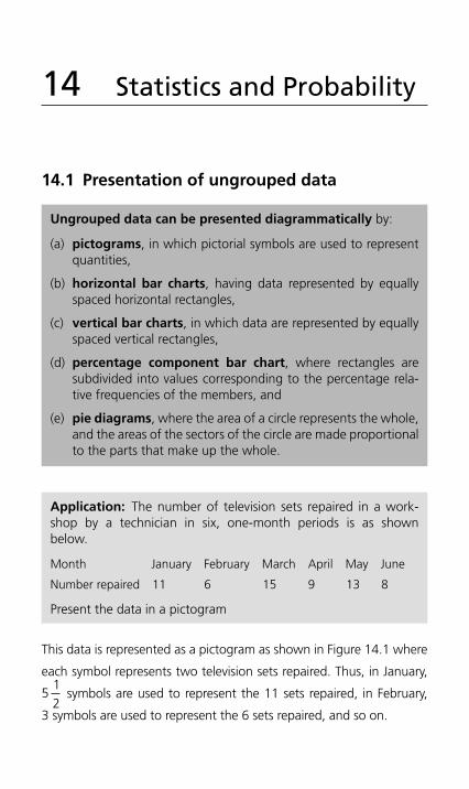
14 Statistics and Probability
This data is represented as a pictogram as shown in Figure 14.1 where
each symbol represents two television sets repaired. Thus, in January,
512
symbols are used to represent the 11 sets repaired, in February,
3 symbols are used to represent the 6 sets repaired, and so on.
Ungrouped data can be presented diagrammatically by:
(a) pictograms, in which pictorial symbols are used to represent quantities,
(b) horizontal bar charts, having data represented by equally spaced horizontal rectangles,
(c) vertical bar charts, in which data are represented by equally spaced vertical rectangles,
(d) percentage component bar chart, where rectangles are subdivided into values corresponding to the percentage rela-tive frequencies of the members, and
(e) pie diagrams, where the area of a circle represents the whole, and the areas of the sectors of the circle are made proportional to the parts that make up the whole.
14.1 Presentation of ungrouped data
Application: The number of television sets repaired in a work-shop by a technician in six, one-month periods is as shown below.
Month January February March April May June
Number repaired 11 6 15 9 13 8
Present the data in a pictogram
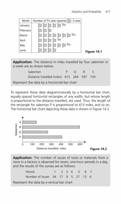
Statistics and Probability 417
To represent these data diagrammatically by a horizontal bar chart, equally spaced horizontal rectangles of any width, but whose length is proportional to the distance travelled, are used. Thus, the length of the rectangle for salesman P is proportional to 413 miles, and so on. The horizontal bar chart depicting these data is shown in Figure 14.2 .
Number of TV sets repairedMonth
January
February
March
April
May
June
2 sets
Figure 14.1
0 100 200 300
Distance travelled, miles
400 500 600
Sal
esm
en
S
R
Q
P
Figure 14.2
Application: The distance in miles travelled by four salesmen in a week are as shown below.
Salesmen P Q R S
Distance travelled (miles) 413 264 597 143
Represent the data by a horizontal bar chart
Application: The number of issues of tools or materials from a store in a factory is observed for seven, one-hour periods in a day, and the results of the survey are as follows:
Period 1 2 3 4 5 6 7
Number of issues 34 17 9 5 27 13 6
Represent the data by a vertical bar chart
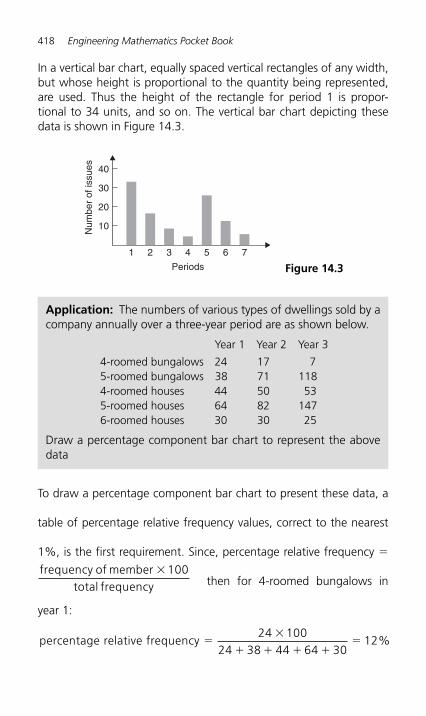
418 Engineering Mathematics Pocket Book
In a vertical bar chart, equally spaced vertical rectangles of any width, but whose height is proportional to the quantity being represented, are used. Thus the height of the rectangle for period 1 is propor-tional to 34 units, and so on. The vertical bar chart depicting these data is shown in Figure 14.3 .
40
30
20
10
1 2 3 4
Periods
5 6 7
Num
ber
of is
sues
Figure 14.3
To draw a percentage component bar chart to present these data, a
table of percentage relative frequency values, correct to the nearest
1%, is the first requirement. Since, percentage relative frequency �
frequency of membertotal frequency
� 100 then for 4-roomed bungalows in
year 1:
percentage relative frequency %��
� � � ��
24 10024 38 44 64 30
12
Application: The numbers of various types of dwellings sold by a company annually over a three-year period are as shown below.
Year 1 Year 2 Year 3
4-roomed bungalows 24 17 7 5-roomed bungalows 38 71 118 4-roomed houses 44 50 53 5-roomed houses 64 82 147 6-roomed houses 30 30 25
Draw a percentage component bar chart to represent the above data
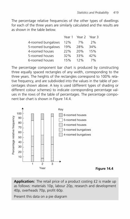
Statistics and Probability 419
The percentage relative frequencies of the other types of dwellings for each of the three years are similarly calculated and the results are as shown in the table below.
Year 1 Year 2 Year 3
4-roomed bungalows 12% 7% 2% 5-roomed bungalows 19% 28% 34% 4-roomed houses 22% 20% 15% 5-roomed houses 32% 33% 42% 6-roomed houses 15% 12% 7%
The percentage component bar chart is produced by constructing three equally spaced rectangles of any width, corresponding to the three years. The heights of the rectangles correspond to 100% rela-tive frequency, and are subdivided into the values in the table of per-centages shown above. A key is used (different types of shading or different colour schemes) to indicate corresponding percentage val-ues in the rows of the table of percentages. The percentage compo-nent bar chart is shown in Figure 14.4 .
100
90
80
70
60
Per
cent
age
rela
tive
freq
uenc
y
50
40
30
20
10
1 2
Year
3
Key
6-roomed houses
5-roomed houses
4-roomed houses
5-roomed bungalows
4-roomed bungalows
Figure 14.4
Application: The retail price of a product costing £2 is made up as follows: materials 10p, labour 20p, research and development 40p, overheads 70p, profit 60 p.
Present this data on a pie diagram
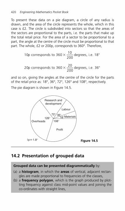
420 Engineering Mathematics Pocket Book
To present these data on a pie diagram, a circle of any radius is drawn, and the area of the circle represents the whole, which in this case is £2. The circle is subdivided into sectors so that the areas of the sectors are proportional to the parts, i.e. the parts that make up the total retail price. For the area of a sector to be proportional to a part, the angle at the centre of the circle must be proportional to that part. The whole, £2 or 200 p, corresponds to 360°. Therefore,
10 36010200
18p corresponds to degrees, i.e. � �
20 36020
200p corresponds to degrees, i.e. 36� �
and so on, giving the angles at the centre of the circle for the parts of the retail price as: 18°, 36°, 72°, 126° and 108°, respectively.
The pie diagram is shown in Figure 14.5 .
Research anddevelopment
Overheads
Profit
Materials
Labour
36°72°126°
108°18°
lp 1.8° Figure 14.5
14.2 Presentation of grouped data
Grouped data can be presented diagrammatically by:
(a) a histogram, in which the areas of vertical, adjacent rectan-gles are made proportional to frequencies of the classes,
(b) a frequency polygon, which is the graph produced by plot-ting frequency against class mid-point values and joining the co-ordinates with straight lines,
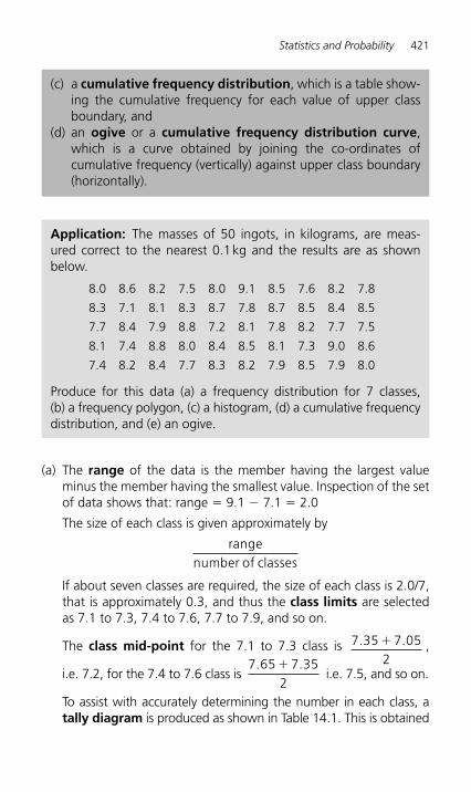
Statistics and Probability 421
(a) The range of the data is the member having the largest value minus the member having the smallest value. Inspection of the set of data shows that: range � 9.1 � 7.1 � 2.0
The size of each class is given approximately by
rangenumber of classes
If about seven classes are required, the size of each class is 2.0/7, that is approximately 0.3, and thus the class limits are selected as 7.1 to 7.3, 7.4 to 7.6, 7.7 to 7.9, and so on.
The class mid-point for the 7.1 to 7.3 class is 7 35 7 052
. .� ,
i.e. 7.2, for the 7.4 to 7.6 class is7 65 7 35
2. .�
i.e. 7.5, and so on.
To assist with accurately determining the number in each class, a tally diagram is produced as shown in Table 14.1 . This is obtained
(c) a cumulative frequency distribution, which is a table show-ing the cumulative frequency for each value of upper class boundary, and
(d) an ogive or a cumulative frequency distribution curve , which is a curve obtained by joining the co-ordinates of cumulative frequency (vertically) against upper class boundary ( horizontally).
Application: The masses of 50 ingots, in kilograms, are meas-ured correct to the nearest 0.1 kg and the results are as shown below.
8.0 8.6 8.2 7.5 8.0 9.1 8.5 7.6 8.2 7.8
8.3 7.1 8.1 8.3 8.7 7.8 8.7 8.5 8.4 8.5
7.7 8.4 7.9 8.8 7.2 8.1 7.8 8.2 7.7 7.5
8.1 7.4 8.8 8.0 8.4 8.5 8.1 7.3 9.0 8.6
7.4 8.2 8.4 7.7 8.3 8.2 7.9 8.5 7.9 8.0
Produce for this data (a) a frequency distribution for 7 classes, (b) a frequency polygon, (c) a histogram, (d) a cumulative frequency distribution, and (e) an ogive.
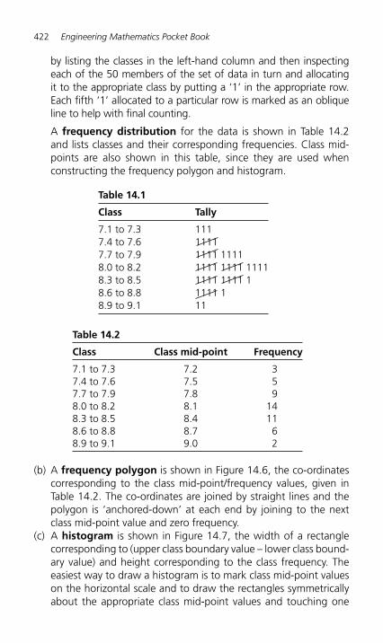
422 Engineering Mathematics Pocket Book
by listing the classes in the left-hand column and then inspecting each of the 50 members of the set of data in turn and allocating it to the appropriate class by putting a ‘ 1 ’ in the appropriate row. Each fifth ‘ 1 ’ allocated to a particular row is marked as an oblique line to help with final counting.
A frequency distribution for the data is shown in Table 14.2 and lists classes and their corresponding frequencies. Class mid-points are also shown in this table, since they are used when constructing the frequency polygon and histogram.
Table 14.2
Class Class mid-point Frequency
7.1 to 7.3 7.2 3 7.4 to 7.6 7.5 5 7.7 to 7.9 7.8 9 8.0 to 8.2 8.1 14 8.3 to 8.5 8.4 11 8.6 to 8.8 8.7 6 8.9 to 9.1 9.0 2
(b) A frequency polygon is shown in Figure 14.6 , the co-ordinates corresponding to the class mid-point/frequency values, given in Table 14.2 . The co-ordinates are joined by straight lines and the polygon is ‘ anchored-down ’ at each end by joining to the next class mid-point value and zero frequency.
(c) A histogram is shown in Figure 14.7 , the width of a rectangle corresponding to (upper class boundary value – lower class bound-ary value) and height corresponding to the class frequency. The easiest way to draw a histogram is to mark class mid-point values on the horizontal scale and to draw the rectangles s ymmetricallyabout the appropriate class mid-point values and touching one
Table 14.1
Class Tally
7.1 to 7.3 111 7.4 to 7.6 1111 7.7 to 7.9 1111 1111 8.0 to 8.2 1111 1111 1111 8.3 to 8.5 1111 1111 1 8.6 to 8.8 1111 1 8.9 to 9.1 11
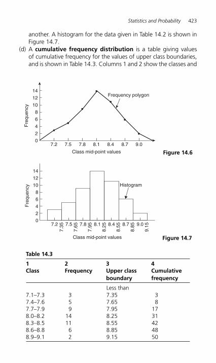
Statistics and Probability 423
14
12
10
8
Fre
quen
cy
6
4
2
07.2 7.5 7.8 8.1
Class mid-point values
Frequency polygon
8.4 8.7 9.0
Figure 14.6
14
12
10
8
Fre
quen
cy Histogram
6
4
2
0
Class mid-point values
7.2 7.5 7.8 8.1 8.4 8.7 9.0
9.15
8.25
8.55
8.85
7.35
7.65
7.95
Figure 14.7
another. A histogram for the data given in Table 14.2 is shown in Figure 14.7 .
(d) A cumulative frequency distribution is a table giving values of cumulative frequency for the values of upper class boundaries, and is shown in Table 14.3 . Columns 1 and 2 show the classes and
Table 14.3
1 2 3 4 Class Frequency Upper class
boundary Cumulative frequency
Less than 7.1–7.3 3 7.35 3 7.4–7.6 5 7.65 8 7.7–7.9 9 7.95 17 8.0–8.2 14 8.25 31 8.3–8.5 11 8.55 42 8.6–8.8 6 8.85 48 8.9–9.1 2 9.15 50
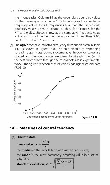
424 Engineering Mathematics Pocket Book
14.3 Measures of central tendency
their frequencies. Column 3 lists the upper class boundary values for the classes given in column 1. Column 4 gives the cumulativefrequency values for all frequencies less than the upper class boundary values given in column 3. Thus, for example, for the 7.7 to 7.9 class shown in row 3, the cumulative frequency value is the sum of all frequencies having values of less than 7.95, i.e. 3 � 5 � 9 � 17, and so on.
(e) The ogive for the cumulative frequency distribution given in Table 14.3 is shown in Figure 14.8 . The co-ordinates corresponding to each upper class boundary/cumulative frequency value are plotted and the co-ordinates are joined by straight lines (– not the best curve drawn through the co-ordinates as in experimental work). The ogive is ‘ anchored ’ at its start by adding the co-o rdinate (7.05, 0).
(a) Discrete data
mean value , xx
n�
∑
the median is the middle term of a ranked set of data,
the mode is the most commonly occurring value in a set of data, and
standard deviation, σ ��( )x x
n
2∑⎧⎨⎪⎪⎪
⎩⎪⎪⎪
⎫⎬⎪⎪⎪
⎭⎪⎪⎪
50
40
30
Cum
ulat
ive
freq
uenc
y
20
10
7.05 7.35 7.65 7.95
Upper class boundary values in kilograms
8.25 8.55 8.85 9.15
Figure 14.8
Statistics and Probability 425
Application: Find the median of the set { 7, 5, 74, 10 }
The set: {7, 5, 74, 10 } is ranked as {5, 7, 10, 74 }, and since it con-tains an even number of members (four in this case), the mean of 7 and 10 is taken, giving a median value of 8.5
Application: Find the median of the set { 3, 81, 15, 7, 14 }
The set: {3, 81, 15, 7, 14 } is ranked as {3, 7, 14, 15, 81 } and the median value is the value of the middle member, i.e. 14
Application: Find the modal value of the set { 5, 6, 8, 2, 5, 4, 6, 5, 3 }
The set: {5, 6, 8, 2, 5, 4, 6, 5, 3 } has a modal value of 5, since the member having a value of 5 occurs three times.
Application: Find the mean, median and modal values for the set { 2, 3, 7, 5, 5, 13, 1, 7, 4, 8, 3, 4, 3 }
For the set { 2, 3, 7, 5, 5, 13, 1, 7, 4, 8, 3, 4, 3 }
mean value
5
,
x_
�� � � � � � � � � � � �
� �2 3 7 5 5 13 1 7 4 8 3 4 3
136513
To obtain the median value the set is ranked, that is, placed in ascend-ing order of magnitude, and since the set contains an odd number of members the value of the middle member is the median value. Ranking the set gives: { 1, 2, 3, 3, 3, 4, 4, 5, 5, 7, 7, 8, 13 }
The middle term is the seventh member, i.e. 4, thus the medianvalue is 4 . The modal value is the value of the most commonly occurring member and is 3, which occurs three times, all other members only occurring once or twice.
Application: Determine the standard deviation from the mean of the set of numbers:
{ 5, 6, 8, 4, 10, 3 } , correct to 4 significant figures
426 Engineering Mathematics Pocket Book
The arithmetic mean, xx
n� �
� � � � ��
∑ 5 6 8 4 10 36
6
Standard deviation, σ ��(x x)
n
2∑⎧⎨⎪⎪⎪
⎩⎪⎪⎪
⎫⎬⎪⎪⎪
⎭⎪⎪⎪
The (x � x ) 2 values are: (5 � 6) 2 , (6 � 6) 2 , (8 � 6) 2 , (4 � 6) 2 , (10 � 6) 2 and (3 � 6) 2
The sum of the (x � x ) 2 values,
i.e. (x x)� 2∑ � 1 � 0 � 4 � 4 � 16 � 9 � 34
and (x x)�
� �2 34
65 6∑
n.i
since there are 6 members in the set.
Hence, standard deviation ,
σ ��
�
�
(x x)
n
, correct to sign
2
5 6
4
∑⎧⎨⎪⎪⎪
⎩⎪⎪⎪
⎫⎬⎪⎪⎪
⎭⎪⎪⎪
.i
2.380 iificant figures.
(b) Grouped data
mean value, x(fx)
f�
∑∑
standard deviation,{f(x x) }
f
2
σ−
�∑
∑⎧⎨⎪⎪⎪
⎩⎪⎪⎪
⎫⎬⎪⎪⎪
⎭⎪⎪⎪
Application: Find (a) the mean value, and (b) the standard deviation for the following values of resistance, in ohms, of 48 resistors:
20.5–20.9 3, 21.0–21.4 10, 21.5–21.9 11,
22.0–22.4 13, 22.5–22.9 9, 23.0–23.4 2
Statistics and Probability 427
(a) The class mid-point/frequency values are:
20.7 3, 21.2 10, 21.7 11, 22.2 13, 22.7 9 and 23.2 2
For grouped data, the mean value is given by: x(f x)
f�
∑∑
where f is the class frequency and x is the class mid-point value. Hence
mean value, x
( ) ( ) ( )
( ) ( ) ( )�
� � � � �
� � � � � �
3 20 7 10 21 2 11 21 7
13 22 2 9 22 7 2 23 2
. . .
. . .448
1052 148
21 919� �.
. ..
i.e. the mean value is 21.9 ohms, correct to 3 significant figures.
(b) From part (a), mean value, x � 21 92. , correct to 4 significant f igures.
The ‘ x-values ’ are the class mid-point values, i.e. 20.7, 21.2, 21.7, … .
Thus the (x � x ) 2 values are (20.7 – 21.92) 2 , (21.2 – 21.92) 2 , (21.7 – 21.92) 2 , … ,
and the f(x � x ) 2 values are 3(20.7 – 21.92) 2 , 10(21.2 – 21.92) 2 , 11(21.7 – 21.92) 2 , … .
The �f(x x)� 2 values are 4.4652 � 5.1840 � 0.5324 � 1.0192 � 5.4756 � 3.2768 � 19.9532
{f(x x) }
f
�� �
2 19 953248
0 41569∑∑
..
and standard deviation,
σ ��
�
�
f(x x)
f
, correct to
2
0 41569{ }⎧
⎨⎪⎪⎪
⎩⎪⎪⎪
⎫⎬⎪⎪⎪
⎭⎪⎪⎪
∑∑
.
0.645 3 significant figures
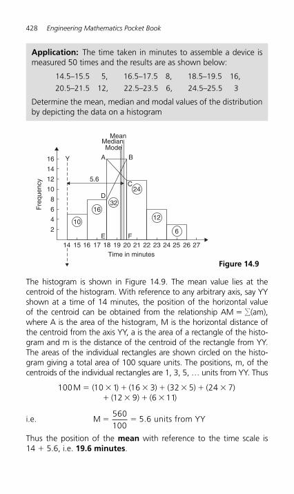
428 Engineering Mathematics Pocket Book
Application: The time taken in minutes to assemble a device is measured 50 times and the results are as shown below:
14.5–15.5 5, 16.5–17.5 8, 18.5–19.5 16,
20.5–21.5 12, 22.5–23.5 6, 24.5–25.5 3
Determine the mean, median and modal values of the d istributionby depicting the data on a histogram
16
12 5.6
MeanMedianMode
A
D
E F
C
BY
10
8
Fre
quen
cy
6
4
2
Time in minutes14 15 16 17 18 19 20 21 2322 24 2625 27
14
106
1216
32
24
Figure 14.9
The histogram is shown in Figure 14.9 . The mean value lies at the centroid of the histogram. With reference to any arbitrary axis, say YY shown at a time of 14 minutes, the position of the horizontal value of the centroid can be obtained from the relationship AM � �(am), where A is the area of the histogram, M is the horizontal distance of the centroid from the axis YY, a is the area of a rectangle of the histo-gram and m is the distance of the centroid of the rectangle from YY. The areas of the individual rectangles are shown circled on the histo-gram giving a total area of 100 square units. The positions, m, of the centroids of the individual rectangles are 1, 3, 5, … units from YY. Thus
100 10 1 16 3 32 5 24 712 9 6 11
M ( ) ( ) ( ) ( )( ) ( )
� � � � � � � �� � � �
i.e. M units from YY� �560100
5 6.
Thus the position of the mean with reference to the time scale is 14 � 5.6, i.e. 19.6 minutes .
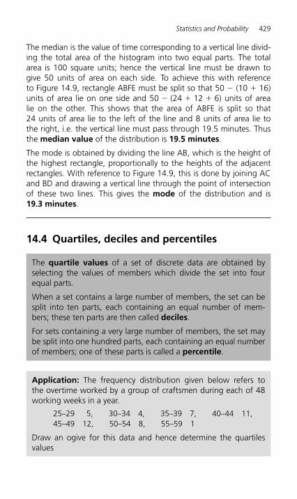
Statistics and Probability 429
The median is the value of time corresponding to a vertical line divid-ing the total area of the histogram into two equal parts. The total area is 100 square units; hence the vertical line must be drawn to give 50 units of area on each side. To achieve this with reference to Figure 14.9 , rectangle ABFE must be split so that 50 � (10 � 16) units of area lie on one side and 50 � (24 � 12 � 6) units of area lie on the other. This shows that the area of ABFE is split so that 24 units of area lie to the left of the line and 8 units of area lie to the right, i.e. the vertical line must pass through 19.5 minutes. Thus the median value of the distribution is 19.5 minutes.
The mode is obtained by dividing the line AB, which is the height of the highest rectangle, proportionally to the heights of the adjacent rectangles. With reference to Figure 14.9, this is done by joining AC and BD and drawing a vertical line through the point of intersection of these two lines. This gives the mode of the distribution and is 19.3 minutes .
The quartile values of a set of discrete data are obtained by selecting the values of members which divide the set into four equal parts.
When a set contains a large number of members, the set can be split into ten parts, each containing an equal number of mem-bers; these ten parts are then called deciles .
For sets containing a very large number of members, the set may be split into one hundred parts, each containing an equal number of members; one of these parts is called a percentile .
14.4 Quartiles, deciles and percentiles
Application: The frequency distribution given below refers to the overtime worked by a group of craftsmen during each of 48 working weeks in a year.
25–29 5, 30–34 4, 35–39 7, 40–44 11, 45–49 12, 50–54 8, 55–59 1
Draw an ogive for this data and hence determine the quartiles values
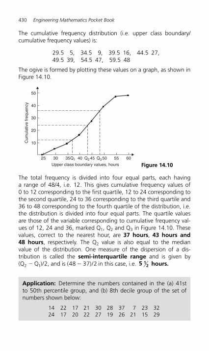
430 Engineering Mathematics Pocket Book
The cumulative frequency distribution (i.e. upper class boundary/cumulative frequency values) is:
29.5 5, 34.5 9, 39.5 16, 44.5 27, 49.5 39, 54.5 47, 59.5 48
The ogive is formed by plotting these values on a graph, as shown in Figure 14.10 .
50
40
30
Cum
ulat
ive
freq
uenc
y
20
10
25 30 35 40
Upper class boundary values, hours
45 50Q3Q2Q1 55 60
Figure 14.10
The total frequency is divided into four equal parts, each having a range of 48/4, i.e. 12. This gives cumulative frequency values of 0 to 12 corresponding to the first quartile, 12 to 24 corresponding to the second quartile, 24 to 36 corresponding to the third quartile and 36 to 48 corresponding to the fourth quartile of the distribution, i.e. the distribution is divided into four equal parts. The quartile values are those of the variable corresponding to cumulative frequency val-ues of 12, 24 and 36, marked Q 1, Q 2 and Q 3 in Figure 14.10 . These values, correct to the nearest hour, are 37 hours, 43 hours and 48 hours, respectively. The Q 2 value is also equal to the median value of the distribution. One measure of the dispersion of a dis-tribution is called the semi-interquartile range and is given by (Q Q2 1 2� )/ , and is ( )48 37 2� / in this case, i.e. 5 1
2 hours.
Application: Determine the numbers contained in the (a) 41st to 50th percentile group, and (b) 8th decile group of the set of numbers shown below:
14 22 17 21 30 28 37 7 23 32 24 17 20 22 27 19 26 21 15 29
Statistics and Probability 431
The set is ranked, giving:
7 14 15 17 17 19 20 21 21 22 22 23 24 26 27 28 29 30 32 37
(a) There are 20 numbers in the set, hence the first 10% will be the two numbers 7 and 14, the second 10% will be 15 and 17, and so on
Thus the 41st to 50th percentile group will be the numbers 21and 22
(b) The first decile group is obtained by splitting the ranked set into 10 equal groups and selecting the first group, i.e. the numbers 7 and 14. The second decile group are the numbers 15 and 17, and so on.
Thus the 8th decile group contains the numbers 27 and 28
14.5 Probability
The probability of events A or B or C or …. . N happening is given by
p p pC NA Bp ....� � � �
The probability of events A and B and C and … N happening is given by
p p p pC NA B....� � � �
Since only one of the ten horses can win, the probability of selecting
at random the winning horse is number of winnersnumber of horses
, i.e. 1
10 or 0.10
Application: Determine the probability of selecting at random the winning horse in a race in which 10 horses are running
Application: Determine the probability of selecting at random the winning horses in both the first and second races if there are 10 horses in each race
432 Engineering Mathematics Pocket Book
The probability of selecting the winning horse in the first race is 110
The probability of selecting the winning horse in the second race
is 110
The probability of selecting the winning horses in the first and second race is given by the multiplication law of probability, i.e.
probability 0.01� � �1
101
101
100or
Application: The probability of a component failing in one year due to excessive temperature is 1
20 , due to excessive vibration is 1
25 and due to excessive humidity is 150 . Determine the probabili-
ties that during a one year period a component: (a) fails due to excessive temperature and excessive vibration, (b) fails due to excessive vibration or excessive humidity, and (c) will not fail due to excessive temperature and excessive humidity
Let p A be the probability of failure due to excessive temperature, then
p and p (where p is the probability of not failiA A A� �1
201920
nng)
Let p B be the probability of failure due to excessive vibration, then
p and pB B� �1
252425
Let p C be the probability of failure due to excessive humidity, then
p and pC C� �1
504950
(a) The probability of a component failing due to excessive tempera-ture and excessive vibration is given by:
p p orA B� � � �1
201
251
5000.002
Statistics and Probability 433
(b) The probability of a component failing due to excessive vibration or excessive humidity is:
p p orB C� � � �1
251
503
500.06
(c) The probability that a component will not fail due to excessive
temperature and will not fail due to excess humidity is:
p p orA C� � � �1920
4950
9311000
0.931
Application: A batch of 40 components contains 5 which are defective. If a component is drawn at random from the batch and tested and then a second component is drawn at random, cal-culate the probability of having one defective component, both with and without replacement.
The probability of having one defective component can be achieved in two ways. If p is the probability of drawing a defective compo-nent and q is the probability of drawing a satisfactory component, then the probability of having one defective component is given by drawing a satisfactory component and then a defective component or by drawing a defective component and then a satisfactory one, i.e. by q � p � p � q
With replacement:
p and q� � � �540
18
3540
78
Hence, probbility of having one defective component is:
18
78
78
18
764
764
� � � � �, i.e. or 7
320.2188
Without replacement:
p 1 � 18
and q 1 � 78
on the first of the two draws. The batch number
is now 39 for the second draw, thus, p 2 � 5
39 and q 2 �
3539
p q q p or 1 2 1 218
3539
78
539
35 35312
� � � � � � �+ 70
3120.2244
434 Engineering Mathematics Pocket Book
14.6 The binomial distribution
If p is the probability that an event will happen and q is the prob-ability that the event will not happen, then the probabilities that the event will happen 0, 1, 2, 3, …, n times in n trials are given by the successive terms of the expansion of (q � p) n, taken from left to right, i.e.
q , nq p, n(n )
!q p ,
n(n )(n )!
q pn n n n� � �� � �1 2 2 3 312
1 23
, ...
Industrial inspection
The probabilities that 0, 1, 2, 3, … , n components are defec-tive in a sample of n components, drawn at random from a large batch of components, are given by the successive terms of the expansion of (q � p) n , taken from left to right.
Application: A dice is rolled 9 times. Find the probabilities of having a 4 upwards (a) 3 times and (b) less than 4 times
Let p be the probability of having a 4 upwards. Then p � 1/6, since dice have six sides.
Let q be the probability of not having a 4 upwards. Then q � 5/6. The probabilities of having a 4 upwards 0, 1, 2.. n times are given by the successive terms of the expansion of (q � p)n, taken from left to right.
From the binomial expansion:
(q � q) 9 � q 9 � 9q 8 p � 36q 7 p 2 � 84q 6 p 3 � ..
The probability of having a 4 upwards no times is q 9 � (5/6) 9 � 0.1938
The probability of having a 4 upwards once is 9q 8 p � 9(5/6) 8 (1/6) � 0.3489
The probability of having a 4 upwards twice is 36q 7 p 2 � 36(5/6) 7 (1/6) 2 � 0.2791
(a) The probability of having a 4 upwards 3 times is 84q 6 p 3 � 84(5/6) 6 (1/6) 3 � 0.1302
Statistics and Probability 435
(b) The probability of having a 4 upwards less than 4 times is the sum of the probabilities of having a 4 upwards 0,1, 2, and 3 times, i.e.
0 1938 0 3489 0 2791 0 1302. . . .� � � � 0.9520
Application: A package contains 50 similar components and inspection shows that four have been damaged during transit. If six components are drawn at random from the contents of the package, determine the probabilities that in this sample (a) one and (b) less than three are damaged
The probability of a component being damaged, p, is 4 in 50, i.e. 0.08 per unit. Thus, the probability of a component not being dam-aged, q, is 1 � 0.08, i.e. 0.92
The probability of there being 0, 1, 2, …, 6 damaged components is given by the successive terms of (q � p) 6 , taken from left to right.
(q p) q q p q p q p ...� � � � � � 6 6 5 4 2 3 36 15 20
(a) The probability of one damaged component is 6q 5 p � 6 � 0.92 5 � 0.08 � 0.3164
(b) The probability of less than three damaged components is given by the sum of the probabilities of 0, 1 and 2 damaged com-ponents, i.e.
q q p q p6 5 4 2 6 5
4 2
6 15 0 92 6 0 92 0 08
15 0 92 0 08
0 6064 0
� � � � � �
� � �
� �
. . .
. .
. .33164 0 0688� �. 0.9916
14.7 The Poisson distribution
If λ is the expectation of the occurrence of an event then the probability of 0, 1, 2, 3, … . occurrences is given by:
e , e , e
!,
e!
,� �� �
λ λλ λ
λ λ λ2 3
2 3...
436 Engineering Mathematics Pocket Book
The sample number, n, is large, the probability of a defective gear-wheel, p, is small and the product np is 80 � 0.03, i.e. 2.4, which is less than 5. Hence a Poisson approximation to a binomial distri-bution may be used. The expectation of a defective gearwheel, λ � np � 2.4
The probabilities of 0, 1, 2, … defective gearwheels are given by
the successive terms of the expression e! !
�� � � �12 3
2 3+
⎛
⎝⎜⎜⎜⎜
⎞
⎠⎟⎟⎟⎟λ
λ λ...
taken from left to right, i.e. by e � λ , λ e � λ , λ λ2
2e!
..�
,
The probability of no defective gearwheels is e �λ � e � 2.4 � 0.0907
The probability of 1 defective gearwheel is λ e �λ � 2.4e � 2.4
� 0.2177
(a) the probability of 2 defective gearwheels is λ λ2 2 2 4
22 4
2 1e!
e� �
��
�
. .
0.2613
(b) The probability of having more than 2 defective gearwheels is 1 – (the sum of the probabilities of having 0, 1, and 2 defective gearwheels), i.e.
1 0 0907 0 2177 0 2613� � �( ), that is, . . . 0.4303
Application: If 3% of the gearwheels produced by a company are defective, determine the probabilities that in a sample of 80 gearwheels (a) two and (b) more than two will be defective
Application: A production department has 35 similar milling machines. The number of breakdowns on each machine averages 0.06 per week. Determine the probabilities of having (a) one, and (b) less than three machines breaking down in any week
Since the average occurrence of a breakdown is known but the number of times when a machine did not break down is unknown, a Poisson distribution must be used.
Statistics and Probability 437
The expectation of a breakdown for 35 machines is 35 � 0.06,i.e. 2.1 breakdowns per week. The probabilities of a breakdown occurring 0, 1, 2, … times are given by the successive terms of the
expression e 1! !
�� � � � �λλ λ2 3
2 3... ,
⎛
⎝⎜⎜⎜⎜
⎞
⎠⎟⎟⎟⎟
taken from left to right.
Hence the probability of no breakdowns e � λ � e � 2.1 � 0.1225
(a) The probability of 1 breakdown is λ e � λ � 2.1e � 2.1 � 0.2572
(b) The probability of 2 breakdowns is λ λ2 2 2 1
22 1
2 1e!
e� �
��
�. .
0.2700
The probability of less than 3 breakdowns per week is the sum of the probabilities of 0, 1 and 2 breakdowns per week,
i.e. 0.1225 � 0.2572 � 0.2700 � 0.6497
14.8 The normal distribution
A table of partial areas under the standardised normal curve is shown in Table 14.4 .
Application: The mean height of 500 people is 170 cm and the standard deviation is 9 cm. Assuming the heights are normally distributed, determine (a) the number of people likely to have heights between 150 cm and 195 cm, (b) the number of people likely to have heights of less than 165 cm, and (c) the number of people likely to have heights of more than 194 cm
(a) The mean value, x_
, is 170 cm and corresponds to a normal stand-
ard variate value, z, of zero on the standardised normal curve.
A height of 150 cm has a z-value given by zx x
��
σ standard
deviations, i.e.150 170
9�
or � 2.22 standard deviations.
Using a table of partial areas beneath the standardised normal curve (see Table 14.4 ), a z-value of �2.22 corresponds to an area of 0.4868 between the mean value and the ordinate z � � 2.22.
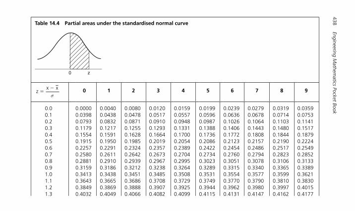
438Engineering M
athematics Pocket Book
Table 14.4 Partial areas under the standardised normal curve
0 z
z
x x�
�
σ 0 1 2 3 4 5 6 7 8 9
0.0 0.0000 0.0040 0.0080 0.0120 0.0159 0.0199 0.0239 0.0279 0.0319 0.0359 0.1 0.0398 0.0438 0.0478 0.0517 0.0557 0.0596 0.0636 0.0678 0.0714 0.0753 0.2 0.0793 0.0832 0.0871 0.0910 0.0948 0.0987 0.1026 0.1064 0.1103 0.1141 0.3 0.1179 0.1217 0.1255 0.1293 0.1331 0.1388 0.1406 0.1443 0.1480 0.1517 0.4 0.1554 0.1591 0.1628 0.1664 0.1700 0.1736 0.1772 0.1808 0.1844 0.1879 0.5 0.1915 0.1950 0.1985 0.2019 0.2054 0.2086 0.2123 0.2157 0.2190 0.2224 0.6 0.2257 0.2291 0.2324 0.2357 0.2389 0.2422 0.2454 0.2486 0.2517 0.2549 0.7 0.2580 0.2611 0.2642 0.2673 0.2704 0.2734 0.2760 0.2794 0.2823 0.2852 0.8 0.2881 0.2910 0.2939 0.2967 0.2995 0.3023 0.3051 0.3078 0.3106 0.3133 0.9 0.3159 0.3186 0.3212 0.3238 0.3264 0.3289 0.3315 0.3340 0.3365 0.3389 1.0 0.3413 0.3438 0.3451 0.3485 0.3508 0.3531 0.3554 0.3577 0.3599 0.3621 1.1 0.3643 0.3665 0.3686 0.3708 0.3729 0.3749 0.3770 0.3790 0.3810 0.3830 1.2 0.3849 0.3869 0.3888 0.3907 0.3925 0.3944 0.3962 0.3980 0.3997 0.4015 1.3 0.4032 0.4049 0.4066 0.4082 0.4099 0.4115 0.4131 0.4147 0.4162 0.4177
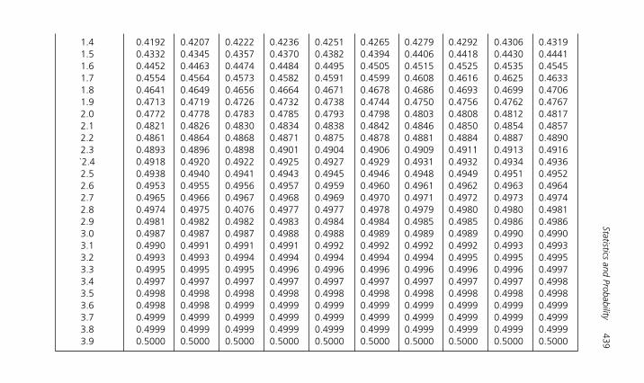
Statistics and Probability 439 1.4 0.4192 0.4207 0.4222 0.4236 0.4251 0.4265 0.4279 0.4292 0.4306 0.4319 1.5 0.4332 0.4345 0.4357 0.4370 0.4382 0.4394 0.4406 0.4418 0.4430 0.4441 1.6 0.4452 0.4463 0.4474 0.4484 0.4495 0.4505 0.4515 0.4525 0.4535 0.4545 1.7 0.4554 0.4564 0.4573 0.4582 0.4591 0.4599 0.4608 0.4616 0.4625 0.4633 1.8 0.4641 0.4649 0.4656 0.4664 0.4671 0.4678 0.4686 0.4693 0.4699 0.4706 1.9 0.4713 0.4719 0.4726 0.4732 0.4738 0.4744 0.4750 0.4756 0.4762 0.4767 2.0 0.4772 0.4778 0.4783 0.4785 0.4793 0.4798 0.4803 0.4808 0.4812 0.4817 2.1 0.4821 0.4826 0.4830 0.4834 0.4838 0.4842 0.4846 0.4850 0.4854 0.4857 2.2 0.4861 0.4864 0.4868 0.4871 0.4875 0.4878 0.4881 0.4884 0.4887 0.4890 2.3 0.4893 0.4896 0.4898 0.4901 0.4904 0.4906 0.4909 0.4911 0.4913 0.4916 ̀2.4 0.4918 0.4920 0.4922 0.4925 0.4927 0.4929 0.4931 0.4932 0.4934 0.4936 2.5 0.4938 0.4940 0.4941 0.4943 0.4945 0.4946 0.4948 0.4949 0.4951 0.4952 2.6 0.4953 0.4955 0.4956 0.4957 0.4959 0.4960 0.4961 0.4962 0.4963 0.4964 2.7 0.4965 0.4966 0.4967 0.4968 0.4969 0.4970 0.4971 0.4972 0.4973 0.4974 2.8 0.4974 0.4975 0.4076 0.4977 0.4977 0.4978 0.4979 0.4980 0.4980 0.4981 2.9 0.4981 0.4982 0.4982 0.4983 0.4984 0.4984 0.4985 0.4985 0.4986 0.4986 3.0 0.4987 0.4987 0.4987 0.4988 0.4988 0.4989 0.4989 0.4989 0.4990 0.4990 3.1 0.4990 0.4991 0.4991 0.4991 0.4992 0.4992 0.4992 0.4992 0.4993 0.4993 3.2 0.4993 0.4993 0.4994 0.4994 0.4994 0.4994 0.4994 0.4995 0.4995 0.4995 3.3 0.4995 0.4995 0.4995 0.4996 0.4996 0.4996 0.4996 0.4996 0.4996 0.4997 3.4 0.4997 0.4997 0.4997 0.4997 0.4997 0.4997 0.4997 0.4997 0.4997 0.4998 3.5 0.4998 0.4998 0.4998 0.4998 0.4998 0.4998 0.4998 0.4998 0.4998 0.4998 3.6 0.4998 0.4998 0.4999 0.4999 0.4999 0.4999 0.4999 0.4999 0.4999 0.4999 3.7 0.4999 0.4999 0.4999 0.4999 0.4999 0.4999 0.4999 0.4999 0.4999 0.4999 3.8 0.4999 0.4999 0.4999 0.4999 0.4999 0.4999 0.4999 0.4999 0.4999 0.4999 3.9 0.5000 0.5000 0.5000 0.5000 0.5000 0.5000 0.5000 0.5000 0.5000 0.5000
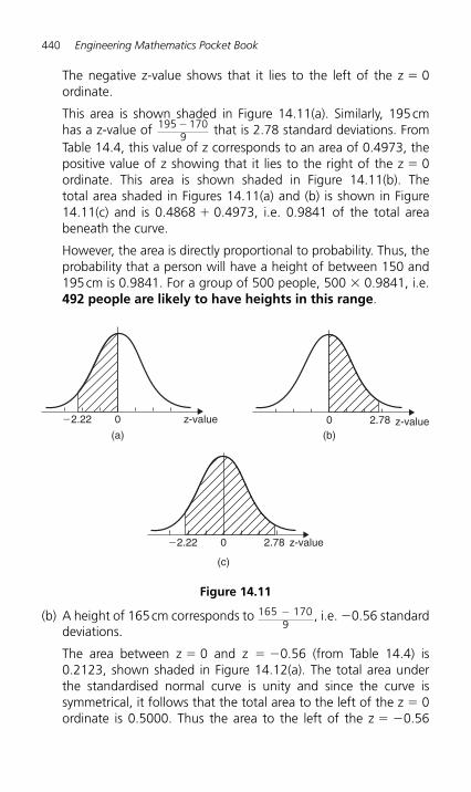
440 Engineering Mathematics Pocket Book
The negative z-value shows that it lies to the left of the z � 0 ordinate.
This area is shown shaded in Figure 14.11(a) . Similarly, 195 cm has a z-value of 195 170
9� that is 2.78 standard deviations. From
Table 14.4 , this value of z corresponds to an area of 0.4973, the positive value of z showing that it lies to the right of the z � 0 ordinate. This area is shown shaded in Figure 14.11(b) . The total area shaded in Figures 14.11(a) and (b) is shown in Figure 14.11(c) and is 0.4868 � 0.4973, i.e. 0.9841 of the total area beneath the curve.
However, the area is directly proportional to probability. Thus, the probability that a person will have a height of between 150 and 195 cm is 0.9841. For a group of 500 people, 500 � 0.9841, i.e. 492 people are likely to have heights in this range .
Figure 14.11
0 z-value�2.22
(a)z-value0 2.78
(b)
z-value0 2.78�2.22
(c)
(b) A height of 165 cm corresponds to 165 1709− , i.e. �0.56 standard
deviations.
The area between z � 0 and z � � 0.56 (from Table 14.4 ) is 0.2123, shown shaded in Figure 14.12(a) . The total area under the standardised normal curve is unity and since the curve is symmetrical, it follows that the total area to the left of the z � 0 ordinate is 0.5000. Thus the area to the left of the z � � 0.56
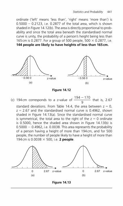
Statistics and Probability 441
ordinate ( ‘ left ’ means ‘less than ’, ‘ right ’ means ‘more than ’) is 0.5000 � 0.2123, i.e. 0.2877 of the total area, which is shown shaded in Figure 14.12(b) . The area is directly proportional to prob-ability and since the total area beneath the standardised normal curve is unity, the probability of a person’s height being less than 165 cm is 0.2877. For a group of 500 people, 500 � 0.2877, i.e. 144 people are likely to have heights of less than 165 cm.
(c) 194 cm corresponds to a z-value of 194 170
9�
that is, 2.67
standard deviations. From Table 14.4 , the area between z � 0, z � 2.67 and the standardised normal curve is 0.4962, shown shaded in Figure 14.13(a) . Since the standardised normal curve is symmetrical, the total area to the right of the z � 0 ordinate is 0.5000, hence the shaded area shown in Figure 14.13(b) is 0.5000 � 0.4962, i.e. 0.0038. This area represents the probability of a person having a height of more than 194 cm, and for 500 people, the number of people likely to have a height of more than 194 cm is 0.0038 � 500, i.e. 2 people.
0�0.56 z-value
(a)
Figure 14.12
0�0.56
(b)
z-value
0 z-value2.67
(a)
Figure 14.13
z-value0 2.67
(b)
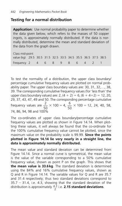
442 Engineering Mathematics Pocket Book
Testing for a normal distribution
Application: Use normal probability paper to determine whether the data given below, which refers to the masses of 50 copper ingots, is approximately normally distributed. If the data is nor-mally distributed, determine the mean and standard deviation of the data from the graph drawn.
Class mid-point value (kg) 29.5 30.5 31.5 32.5 33.5 34.5 35.5 36.5 37.5 38.5
Frequency 2 4 6 8 9 8 6 4 2 1
To test the normality of a distribution, the upper class boundary/percentage cumulative frequency values are plotted on normal prob-ability paper. The upper class boundary values are: 30, 31, 32, …, 38, 39. The corresponding cumulative frequency values (for ‘less than ’ the upper class boundary values) are: 2, (4 � 2) � 6, (6 � 4�2) � 12, 20, 29, 37, 43, 47, 49 and 50. The corresponding percentage cumulative
frequency values are 2
50 � 100 � 4,
650
� 100 � 12, 24, 40, 58,
74, 86, 94, 98 and 100%
The co-ordinates of upper class boundary/percentage cumulative frequency values are plotted as shown in Figure 14.14 . When plot-ting these values, it will always be found that the co-ordinate for the 100% cumulative frequency value cannot be plotted, since the maximum value on the probability scale is 99.99. Since the points plotted in Figure 14.14 lie very nearly in a straight line, the data is approximately normally distributed.
The mean value and standard deviation can be determined from Figure 14.14 . Since a normal curve is symmetrical, the mean value is the value of the variable corresponding to a 50% cumulative frequency value, shown as point P on the graph. This shows that the mean value is 33.6 kg. The standard deviation is determined using the 84% and 16% cumulative frequency values, shown as Q and R in Figure 14.14 . The variable values for Q and R are 35.7 and 31.4 respectively; thus two standard deviations correspond to 35.7 � 31.4, i.e. 4.3, showing that the standard deviation of the distribution is approximately 4 3
2. i.e. 2.15 standard deviations.
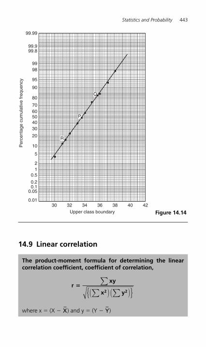
Statistics and Probability 443
14.9 Linear correlation
The product-moment formula for determining the linear correlation coefficient, coefficient of correlation,
rxy
x y2 2�
∑∑ ∑( )( ){ }
where x � (X � X ) and y � (Y � Y )
30 32 34 36 38 40 420.01
0.050.10.2
0.512
5
10
20
3040506070
80
90
95
9899
99.899.9
99.99
Per
cent
age
cum
ulat
ive
freq
uenc
y
Upper class boundary
Q
P
R
Figure 14.14
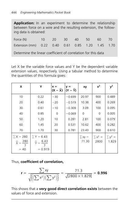
444 Engineering Mathematics Pocket Book
Let X be the variable force values and Y be the dependent variable extension values, respectively. Using a tabular method to determine the quantities of this formula gives:
X Y x � (X � X )
y � (Y � Y )
xy x2 y2
10 0.22 �30 � 0.699 20.97 900 0.489
20 0.40 �20 � 0.519 10.38 400 0.269
30 0.61 �10 � 0.309 3.09 100 0.095
40 0.85 0 � 0.069 0 0 0.005
50 1.20 10 0.281 2.81 100 0.079
60 1.45 20 0.531 10.62 400 0.282
70 1.70 30 0.781 23.43 900 0.610
� X
X
�
�
�
280
2807
40
� Y
Y
�
�
�
6 43
6 437
0 919
.
.
.
� xy �
71 30.
� x2
2800
�
� y2
1 829
�
.
Application: In an experiment to determine the relationship between force on a wire and the resulting extension, the follow-ing data is obtained:
Force (N) 10 20 30 40 50 60 70
Extension (mm) 0.22 0.40 0.61 0.85 1.20 1.45 1.70
Determine the linear coefficient of correlation for this data
Thus, coefficient of correlation,
r �
xy
x y [ ]∑
∑ ∑( )( ){ }2 2
71 3
2800 1 829�
��
.
.0.996
This shows that a very good direct correlation exists between the values of force and extension.
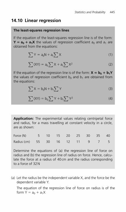
Statistics and Probability 445
14.10 Linear regression
The least-squares regression lines
If the equation of the least-squares regression line is of the form: Y � a 0 � a 1 X the values of regression coefficient a 0 and a 1 are obtained from the equations:
Y a N a X∑ ∑� �0 1 (1)
(XY) a X a X∑ ∑ ∑� �0 12 (2)
If the equation of the regression line is of the form: X � b 0 � b 1 Y the values of regression coefficient b 0 and b 1 are obtained from the equations:
X b N b Y� �0 1∑∑ (3)
(XY) b Y b Y∑ ∑ ∑� �0 12 (4)
Application: The experimental values relating centripetal force and radius, for a mass travelling at constant velocity in a circle, are as shown:
Force (N) 5 10 15 20 25 30 35 40
Radius (cm) 55 30 16 12 11 9 7 5
Determine the equations of (a) the regression line of force on radius and (b) the regression line of radius on force. Hence, calcu-late the force at a radius of 40 cm and the radius corresponding to a force of 32 N
(a) Let the radius be the independent variable X, and the force be the dependent variable Y.
The equation of the regression line of force on radius is of the form Y � a 0 � a 1 X
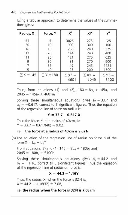
446 Engineering Mathematics Pocket Book
Using a tabular approach to determine the values of the summa-tions gives:
Radius, X Force, Y X 2 XY Y2
55 5 3025 275 25 30 10 900 300 100 16 15 256 240 225 12 20 144 240 400 11 25 121 275 625 9 30 81 270 900 7 35 49 245 1225 5 40 25 200 1600
� X � 145 � Y � 180
� X2
4601�
� XY �2045
� Y2
5100�
Thus, from equations (1) and (2), 180 � 8a 0 � 145a 1 and 2045 � 145a 0 � 4601a 1
Solving these simultaneous equations gives a 0 � 33.7 and a1 � � 0.617, correct to 3 significant figures. Thus the equation of the regression line of force on radius is:
Y 33.7 0.617 X� � Thus the force, Y, at a radius of 40 cm, is: Y � 33.7 � 0.617(40) � 9.02
i.e. the force at a radius of 40 cm is 9.02 N
(b) The equation of the regression line of radius on force is of the form X � b 0 � b 1 Y
From equations (3) and (4), 145 � 8b 0 � 180b 1 and 2045 � 180b 0 � 5100b 1
Solving these simultaneous equations gives b 0 � 44.2 and b1 � � 1.16, correct to 3 significant figures. Thus the equation of the regression line of radius on force is:
X 44.2 1.16Y� � Thus, the radius, X, when the force is 32 N is: X � 44.2 � 1.16(32) � 7.08,
i.e. the radius when the force is 32 N is 7.08 cm
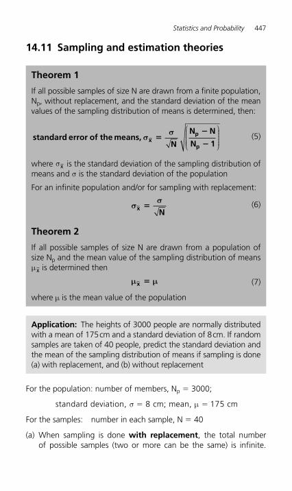
Statistics and Probability 447
14.11 Sampling and estimation theories
Theorem 1
If all possible samples of size N are drawn from a finite population, Np, without replacement, and the standard deviation of the mean values of the sampling distribution of means is determined, then:
standard error of the means, N
N N
N 1xp
p
σσ
��
�
⎛
⎝
⎜⎜⎜⎜⎜
⎞
⎠
⎟⎟⎟⎟⎟(5)
where σx is the standard deviation of the sampling distribution of means and σ is the standard deviation of the population
For an infinite population and/or for sampling with replacement:
σσ
x �N
(6)
Theorem 2
If all possible samples of size N are drawn from a population of size N p and the mean value of the sampling distribution of means μx is determined then
μ μx � (7)
where μ is the mean value of the population
Application: The heights of 3000 people are normally distributed with a mean of 175 cm and a standard deviation of 8 cm. If random samples are taken of 40 people, predict the standard deviation and the mean of the sampling distribution of means if sampling is done (a) with replacement, and (b) without replacement
For the population: number of members, N p � 3000;
standard deviation, cm; mean, cmσ μ� �8 175 For the samples: number in each sample, N � 40
(a) When sampling is done with replacement, the total number of possible samples (two or more can be the same) is infinite.
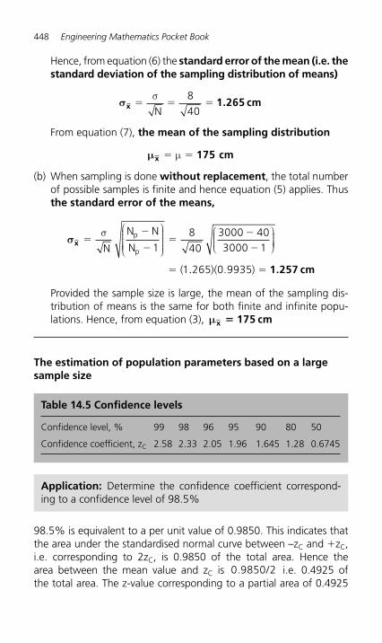
448 Engineering Mathematics Pocket Book
Hence, from equation (6) the standard error of the mean (i.e. the standard deviation of the sampling distribution of means)
σx 1.265 cm� � �σN
8
40
From equation (7), the mean of the sampling distribution
μx 175 cm� �μ (b) When sampling is done without replacement, the total number
of possible samples is finite and hence equation (5) applies. Thus the standard error of the means,
σx ��
��
�
�
�
σN
N N
N
(
p
p 18
40
3000 403000 1
1
⎛
⎝
⎜⎜⎜⎜⎜
⎞
⎠
⎟⎟⎟⎟⎟
⎛⎝⎜⎜⎜
⎞⎠⎟⎟⎟⎟
.. .265 0 9935)( ) � 1.257 cm
Provided the sample size is large, the mean of the sampling dis-tribution of means is the same for both finite and infinite popu-lations. Hence, from equation (3), μx 175 cm�
The estimation of population parameters based on a large sample size
Table 14.5 Confidence levels
Confidence level, % 99 98 96 95 90 80 50
Confidence coefficient, z C 2.58 2.33 2.05 1.96 1.645 1.28 0.6745
Application: Determine the confidence coefficient correspond-ing to a confidence level of 98.5%
98.5% is equivalent to a per unit value of 0.9850. This indicates that the area under the standardised normal curve between –z C and � zC , i.e. corresponding to 2z C, is 0.9850 of the total area. Hence the area between the mean value and z C is 0 9850 2. / i.e. 0.4925 of the total area. The z-value corresponding to a partial area of 0.4925
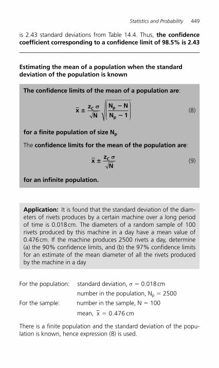
Statistics and Probability 449
is 2.43 standard deviations from Table 14.4 . Thus, the confidence coefficient corresponding to a confidence limit of 98.5% is 2.43
Estimating the mean of a population when the standard deviation of the population is known
The confidence limits of the mean of a population are :
xz
N
N N
N 1C p
p
��
�
σ ⎛
⎝
⎜⎜⎜⎜⎜
⎞
⎠
⎟⎟⎟⎟⎟(8)
for a finite population of size N p
The confidence limits for the mean of the population are :
xz
NC�
σ(9)
for an infinite population.
Application: It is found that the standard deviation of the diam-eters of rivets produces by a certain machine over a long period of time is 0.018 cm. The diameters of a random sample of 100 rivets produced by this machine in a day have a mean value of 0.476 cm. If the machine produces 2500 rivets a day, determine (a) the 90% confidence limits, and (b) the 97% confidence limits for an estimate of the mean diameter of all the rivets produced by the machine in a day
For the population: standard deviation, σ � 0.018 cm
number in the population, N p � 2500
For the sample: number in the sample, N � 100
mean, x cm� 0 476.
There is a finite population and the standard deviation of the popu-lation is known, hence expression (8) is used.
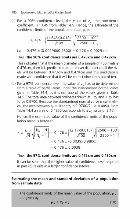
450 Engineering Mathematics Pocket Book
(a) For a 90% confidence level, the value of z C , the confidence coefficient, is 1.645 from Table 14.5 . Hence, the estimate of the confidence limits of the population mean, μ , is:
0 4761 645 0 018
100
2500 1002500 1
.. .
�
�
( )( )⎛
⎝⎜⎜⎜⎜
⎞
⎠⎟⎟⎟⎟
⎛⎝⎜⎜⎜
⎞⎠⎟⎟⎟⎟⎟
i.e. 0 476 0 00296 0 9800 0 476 0 0029. . . . . � ( )( ) cm Thus, the 90% confidence limits are 0.473 cm and 0.479 cm
This indicates that if the mean diameter of a sample of 100 rivets is 0.476 cm, then it is predicted that the mean diameter of all the riv-ets will be between 0.473 cm and 0.479 cm and this prediction is made with confidence that it will be correct nine times out of ten.
(b) For a 97% confidence level, the value of z C has to be determined from a table of partial areas under the standardised normal curve given in Table 14.4 , as it is not one of the values given in Table 14.5. The total area between ordinates drawn at �zC and � zC has to be 0.9700. Because the standardised normal curve is symmetri-cal, the area between z C � 0 and z C is 0 9700 2. / , i.e. 0.4850. From Table 14.4 an area of 0.4850 corresponds to a z C value of 2.17.
Hence, the estimated value of the confidence limits of the popu-lation mean is between
xz
N
N N
NC p
p
�
��
σ1
0 4762 17 0 018
100
⎛
⎝
⎜⎜⎜⎜⎜
⎞
⎠
⎟⎟⎟⎟⎟
⎛
⎝⎜⎜⎜⎜
⎞.
( . )( . )
⎠⎠⎟⎟⎟⎟
⎛⎝⎜⎜⎜
⎞⎠⎟⎟⎟⎟
2500 1002500 1
0 476 0 0039 0 9800
0 4
�
�
�
�
. . .
.
( )( )
776 0 0038 .
Thus, the 97% confidence limits are 0.472 cm and 0.480 cm
It can be seen that the higher value of confidence level required in part (b) results in a larger confidence interval.
Estimating the mean and standard deviation of a population from sample data
The confidence limits of the mean value of the population, μ , are given by:
μ σx C xz� (10)
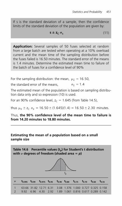
Statistics and Probability 451
For the sampling distribution: the mean, μ x � 16 50. ,
the standard error of the means, σx � 1 4.
The estimated mean of the population is based on sampling distribu-tion data only and so expression (10) is used.
For an 90% confidence level, z C � 1.645 (from Table 14.5 ),
thus μ σx C xz ( )( ) � � 16 50 1 645 1 4 16 50 2 30. . . . . minutes.
Thus, the 90% confidence level of the mean time to failure is from 14.20 minutes to 18.80 minutes.
Estimating the mean of a population based on a small sample size
If s is the standard deviation of a sample, then the confidence limits of the standard deviation of the population are given by:
s zC s� σ (11)
Application: Several samples of 50 fuses selected at random from a large batch are tested when operating at a 10% overload current and the mean time of the sampling distribution before the fuses failed is 16.50 minutes. The standard error of the means is 1.4 minutes. Determine the estimated mean time to failure of the batch of fuses for a confidence level of 90%
Table 14.6 Percentile values (t p ) for Student’s t distribution with ν degrees of freedom (shaded area � p )
tp
ν t 0.995 t0.99 t0.975 t0.95 t0.90 t0.80 t0.75 t0.70 t0.60 t0.55
1 63.66 31.82 12.71 6.31 3.08 1.376 1.000 0.727 0.325 0.158 2 9.92 6.96 4.30 2.92 1.89 1.061 0.816 0.617 0.289 0.142
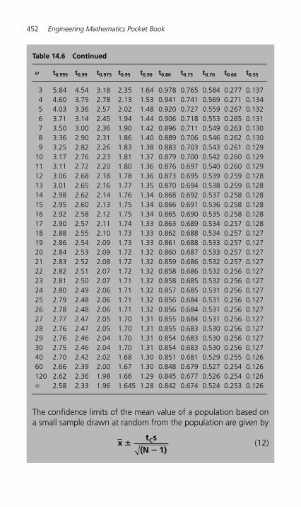
452 Engineering Mathematics Pocket Book
Table 14.6 Continued
ν t 0.995 t0.99 t0.975 t0.95 t0.90 t0.80 t0.75 t0.70 t0.60 t0.55
3 5.84 4.54 3.18 2.35 1.64 0.978 0.765 0.584 0.277 0.137 4 4.60 3.75 2.78 2.13 1.53 0.941 0.741 0.569 0.271 0.134 5 4.03 3.36 2.57 2.02 1.48 0.920 0.727 0.559 0.267 0.132 6 3.71 3.14 2.45 1.94 1.44 0.906 0.718 0.553 0.265 0.131 7 3.50 3.00 2.36 1.90 1.42 0.896 0.711 0.549 0.263 0.130 8 3.36 2.90 2.31 1.86 1.40 0.889 0.706 0.546 0.262 0.130 9 3.25 2.82 2.26 1.83 1.38 0.883 0.703 0.543 0.261 0.129 10 3.17 2.76 2.23 1.81 1.37 0.879 0.700 0.542 0.260 0.129 11 3.11 2.72 2.20 1.80 1.36 0.876 0.697 0.540 0.260 0.129 12 3.06 2.68 2.18 1.78 1.36 0.873 0.695 0.539 0.259 0.128 13 3.01 2.65 2.16 1.77 1.35 0.870 0.694 0.538 0.259 0.128 14 2.98 2.62 2.14 1.76 1.34 0.868 0.692 0.537 0.258 0.128 15 2.95 2.60 2.13 1.75 1.34 0.866 0.691 0.536 0.258 0.128 16 2.92 2.58 2.12 1.75 1.34 0.865 0.690 0.535 0.258 0.128 17 2.90 2.57 2.11 1.74 1.33 0.863 0.689 0.534 0.257 0.128 18 2.88 2.55 2.10 1.73 1.33 0.862 0.688 0.534 0.257 0.127 19 2.86 2.54 2.09 1.73 1.33 0.861 0.688 0.533 0.257 0.127 20 2.84 2.53 2.09 1.72 1.32 0.860 0.687 0.533 0.257 0.127 21 2.83 2.52 2.08 1.72 1.32 0.859 0.686 0.532 0.257 0.127 22 2.82 2.51 2.07 1.72 1.32 0.858 0.686 0.532 0.256 0.127 23 2.81 2.50 2.07 1.71 1.32 0.858 0.685 0.532 0.256 0.127 24 2.80 2.49 2.06 1.71 1.32 0.857 0.685 0.531 0.256 0.127 25 2.79 2.48 2.06 1.71 1.32 0.856 0.684 0.531 0.256 0.127 26 2.78 2.48 2.06 1.71 1.32 0.856 0.684 0.531 0.256 0.127 27 2.77 2.47 2.05 1.70 1.31 0.855 0.684 0.531 0.256 0.127 28 2.76 2.47 2.05 1.70 1.31 0.855 0.683 0.530 0.256 0.127 29 2.76 2.46 2.04 1.70 1.31 0.854 0.683 0.530 0.256 0.127 30 2.75 2.46 2.04 1.70 1.31 0.854 0.683 0.530 0.256 0.127 40 2.70 2.42 2.02 1.68 1.30 0.851 0.681 0.529 0.255 0.126 60 2.66 2.39 2.00 1.67 1.30 0.848 0.679 0.527 0.254 0.126 120 2.62 2.36 1.98 1.66 1.29 0.845 0.677 0.526 0.254 0.126 � 2.58 2.33 1.96 1.645 1.28 0.842 0.674 0.524 0.253 0.126
The confidence limits of the mean value of a population based on a small sample drawn at random from the population are given by
xt s
(N 1)C��
(12)
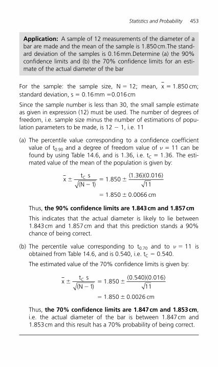
Statistics and Probability 453
For the sample: the sample size, N � 12; mean, x cm;� 1 850. standard deviation, s � 0.16 mm � 0.016 cm
Since the sample number is less than 30, the small sample estimate as given in expression (12) must be used. The number of degrees of freedom, i.e. sample size minus the number of estimations of popu-lation parameters to be made, is 12 � 1, i.e. 11
(a) The percentile value corresponding to a confidence coefficient value of t 0.90 and a degree of freedom value of ν � 11 can be found by using Table 14.6 , and is 1.36, i.e. t C � 1.36. The esti-mated value of the mean of the population is given by:
xt
(N )
( )( )
cm
C �
�
�
s
11 850
1 36 0 016
11
1 850 0 0066
.. .
. .
Thus, the 90% confidence limits are 1.843 cm and 1.857 cm
This indicates that the actual diameter is likely to lie between 1.843 cm and 1.857 cm and that this prediction stands a 90% chance of being correct.
(b) The percentile value corresponding to t 0.70 and to ν � 11 is obtained from Table 14.6 , and is 0.540, i.e. t C � 0.540.
The estimated value of the 70% confidence limits is given by:
xt s
(N )
( )( )
cm
C �
�
�
11 850
0 540 0 016
11
1 850 0 0026
.. .
. .
Thus, the 70% confidence limits are 1.847 cm and 1.853 cm, i.e. the actual diameter of the bar is between 1.847 cm and 1.853 cm and this result has a 70% probability of being correct.
Application: A sample of 12 measurements of the diameter of a bar are made and the mean of the sample is 1.850 cm.The stand-ard deviation of the samples is 0.16 mm.Determine (a) the 90% confidence limits and (b) the 70% confidence limits for an esti-mate of the actual diameter of the bar
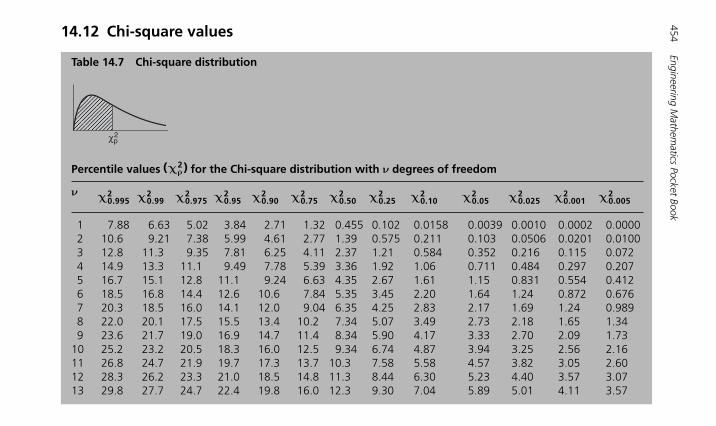
454Engineering M
athematics Pocket Book
Table 14.7 Chi-square distribution
χp
2
Percentile values ( )2χ ρ for the Chi-square distribution with ν degrees of freedom
ν χ0.9952 χ0.99
2 χ0.9752 χ0.95
2 χ0.902 χ0.75
2 χ0.502 χ0.25
2 χ0.102 χ0.05
2 χ0.0252 χ0.001
2 χ0.0052
1 7.88 6.63 5.02 3.84 2.71 1.32 0.455 0.102 0.0158 0.0039 0.0010 0.0002 0.0000 2 10.6 9.21 7.38 5.99 4.61 2.77 1.39 0.575 0.211 0.103 0.0506 0.0201 0.0100 3 12.8 11.3 9.35 7.81 6.25 4.11 2.37 1.21 0.584 0.352 0.216 0.115 0.072 4 14.9 13.3 11.1 9.49 7.78 5.39 3.36 1.92 1.06 0.711 0.484 0.297 0.207 5 16.7 15.1 12.8 11.1 9.24 6.63 4.35 2.67 1.61 1.15 0.831 0.554 0.412 6 18.5 16.8 14.4 12.6 10.6 7.84 5.35 3.45 2.20 1.64 1.24 0.872 0.676 7 20.3 18.5 16.0 14.1 12.0 9.04 6.35 4.25 2.83 2.17 1.69 1.24 0.989 8 22.0 20.1 17.5 15.5 13.4 10.2 7.34 5.07 3.49 2.73 2.18 1.65 1.34 9 23.6 21.7 19.0 16.9 14.7 11.4 8.34 5.90 4.17 3.33 2.70 2.09 1.73 10 25.2 23.2 20.5 18.3 16.0 12.5 9.34 6.74 4.87 3.94 3.25 2.56 2.16 11 26.8 24.7 21.9 19.7 17.3 13.7 10.3 7.58 5.58 4.57 3.82 3.05 2.60 12 28.3 26.2 23.3 21.0 18.5 14.8 11.3 8.44 6.30 5.23 4.40 3.57 3.07 13 29.8 27.7 24.7 22.4 19.8 16.0 12.3 9.30 7.04 5.89 5.01 4.11 3.57
14.12 Chi-square values
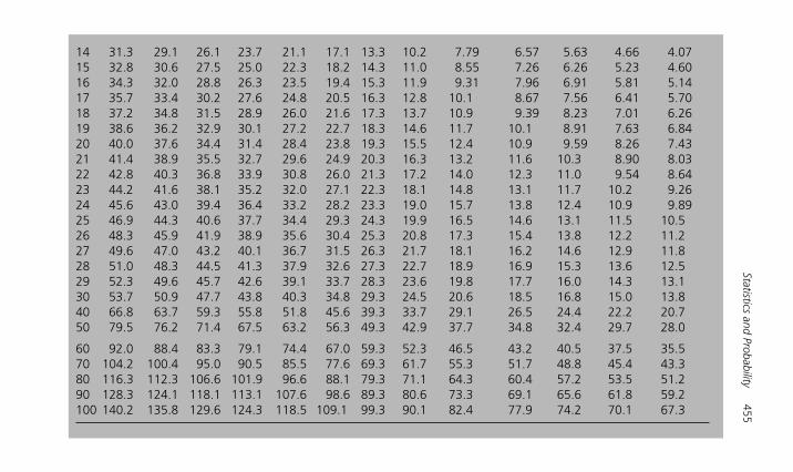
Statistics and Probability 455 14 31.3 29.1 26.1 23.7 21.1 17.1 13.3 10.2 7.79 6.57 5.63 4.66 4.07 15 32.8 30.6 27.5 25.0 22.3 18.2 14.3 11.0 8.55 7.26 6.26 5.23 4.60 16 34.3 32.0 28.8 26.3 23.5 19.4 15.3 11.9 9.31 7.96 6.91 5.81 5.14 17 35.7 33.4 30.2 27.6 24.8 20.5 16.3 12.8 10.1 8.67 7.56 6.41 5.70 18 37.2 34.8 31.5 28.9 26.0 21.6 17.3 13.7 10.9 9.39 8.23 7.01 6.26 19 38.6 36.2 32.9 30.1 27.2 22.7 18.3 14.6 11.7 10.1 8.91 7.63 6.84 20 40.0 37.6 34.4 31.4 28.4 23.8 19.3 15.5 12.4 10.9 9.59 8.26 7.43 21 41.4 38.9 35.5 32.7 29.6 24.9 20.3 16.3 13.2 11.6 10.3 8.90 8.03 22 42.8 40.3 36.8 33.9 30.8 26.0 21.3 17.2 14.0 12.3 11.0 9.54 8.64 23 44.2 41.6 38.1 35.2 32.0 27.1 22.3 18.1 14.8 13.1 11.7 10.2 9.26 24 45.6 43.0 39.4 36.4 33.2 28.2 23.3 19.0 15.7 13.8 12.4 10.9 9.89 25 46.9 44.3 40.6 37.7 34.4 29.3 24.3 19.9 16.5 14.6 13.1 11.5 10.5 26 48.3 45.9 41.9 38.9 35.6 30.4 25.3 20.8 17.3 15.4 13.8 12.2 11.2 27 49.6 47.0 43.2 40.1 36.7 31.5 26.3 21.7 18.1 16.2 14.6 12.9 11.8 28 51.0 48.3 44.5 41.3 37.9 32.6 27.3 22.7 18.9 16.9 15.3 13.6 12.5 29 52.3 49.6 45.7 42.6 39.1 33.7 28.3 23.6 19.8 17.7 16.0 14.3 13.1 30 53.7 50.9 47.7 43.8 40.3 34.8 29.3 24.5 20.6 18.5 16.8 15.0 13.8 40 66.8 63.7 59.3 55.8 51.8 45.6 39.3 33.7 29.1 26.5 24.4 22.2 20.7 50 79.5 76.2 71.4 67.5 63.2 56.3 49.3 42.9 37.7 34.8 32.4 29.7 28.0
60 92.0 88.4 83.3 79.1 74.4 67.0 59.3 52.3 46.5 43.2 40.5 37.5 35.5 70 104.2 100.4 95.0 90.5 85.5 77.6 69.3 61.7 55.3 51.7 48.8 45.4 43.3 80 116.3 112.3 106.6 101.9 96.6 88.1 79.3 71.1 64.3 60.4 57.2 53.5 51.2 90 128.3 124.1 118.1 113.1 107.6 98.6 89.3 80.6 73.3 69.1 65.6 61.8 59.2 100 140.2 135.8 129.6 124.3 118.5 109.1 99.3 90.1 82.4 77.9 74.2 70.1 67.3
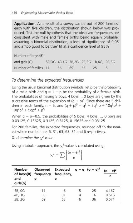
456 Engineering Mathematics Pocket Book
To determine the expected frequencies
Using the usual binomial distribution symbols, let p be the probability of a male birth and q � 1 � p be the probability of a female birth. The probabilities of having 5 boys, 4 boys,.., 0 boys are given by the successive terms of the expansion of (q � p) n. Since there are 5 chil-dren in each family, n � 5, and (q � p) 5 � q 5 � 5q 4 p � 10q 3 p 2 � 10q 2 p 3 � 5qp 4 � p 5
When q � p �0.5, the probabilities of 5 boys, 4 boys, …, 0 boys are 0.03125, 0.15625, 0.3125, 0.3125, 0.15625 and 0.03125
For 200 families, the expected frequencies, rounded off to the near-est whole number are: 6, 31, 63, 63, 31 and 6 respectively.
To determine the χ 2 -value
Using a tabular approach, the χ 2 -value is calculated using
χο2
2�
�( )ee
⎧⎨⎪⎪⎩⎪⎪
⎫⎬⎪⎪⎭⎪⎪
∑
Number of boys(B) and girls(G)
Observed frequency,o
Expected frequency,e
o � e (o � e) 2
(o e)
e
2�
5B, 0G 11 6 5 25 4.167 4B, 1G 35 31 4 16 0.516 3B, 2G 69 63 6 36 0.571
Application: As a result of a survey carried out of 200 families, each with five children, the distribution shown below was pro-duced. Test the null hypothesis that the observed frequencies are consistent with male and female births being equally probable, assuming a binomial distribution, a level of significance of 0.05 and a ‘ too good to be true ’ fit at a confidence level of 95%
Number of boys (B)
and girls (G) 5B,OG 4B,1G 3B,2G 2B,3G 1B,4G, 0B,5G
Number of families 11 35 69 55 25 5
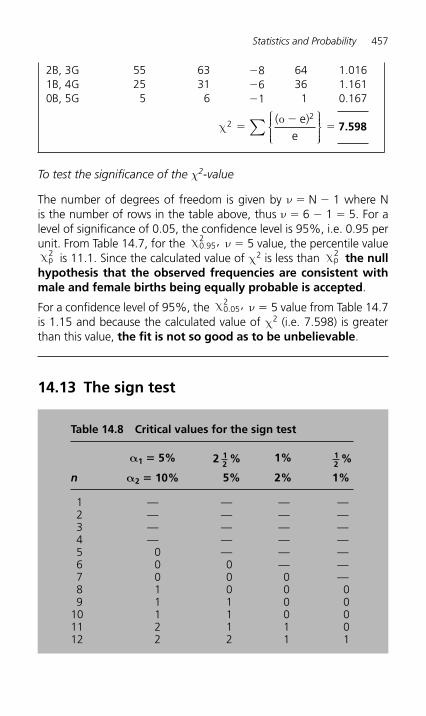
Statistics and Probability 457
2B, 3G 55 63 � 8 64 1.016 1B, 4G 25 31 � 6 36 1.161 0B, 5G 5 6 � 1 1 0.167
χ
ο22
��( )ee
⎧⎨⎪⎪⎩⎪⎪
⎫⎬⎪⎪⎭⎪⎪
∑ � 7.598
To test the significance of the χ 2 -value
The number of degrees of freedom is given by ν � N � 1 where N is the number of rows in the table above, thus ν � 6 � 1 � 5. For a level of significance of 0.05, the confidence level is 95%, i.e. 0.95 per unit. From Table 14.7 , for the χ0 95
2. , ν � 5 value, the percentile value
χp2 is 11.1. Since the calculated value of χ 2 is less than χp
2 the null hypothesis that the observed frequencies are consistent with male and female births being equally probable is accepted .
For a confidence level of 95%, the χ0 052
. , ν � 5 value from Table 14.7 is 1.15 and because the calculated value of χ 2 (i.e. 7.598) is greater than this value, the fit is not so good as to be unbelievable.
14.13 The sign test
Table 14.8 Critical values for the sign test
α 1 � 5% 2 %12
1% 12 %
n α 2 � 10% 5% 2% 1%
1 — — — — 2 — — — — 3 — — — — 4 — — — — 5 0 — — — 6 0 0 — — 7 0 0 0 — 8 1 0 0 0 9 1 1 0 0
10 1 1 0 0 11 2 1 1 0 12 2 2 1 1
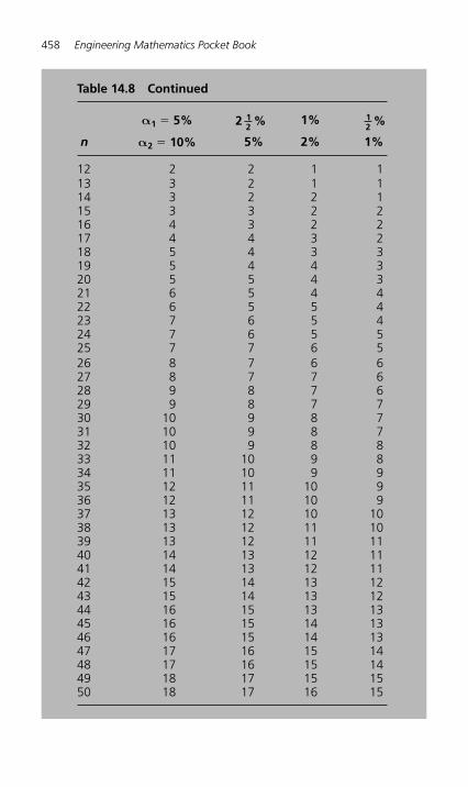
458 Engineering Mathematics Pocket Book
Table 14.8 Continued
α 1 � 5% 2 %12
1% 12 %
n α 2 � 10% 5% 2% 1%
12 2 2 1 1 13 3 2 1 1 14 3 2 2 1 15 3 3 2 2 16 4 3 2 2 17 4 4 3 2 18 5 4 3 3 19 5 4 4 3 20 5 5 4 3 21 6 5 4 4 22 6 5 5 4 23 7 6 5 4 24 7 6 5 5 25 7 7 6 526 8 7 6 627 8 7 7 628 9 8 7 629 9 8 7 730 10 9 8 731 10 9 8 732 10 9 8 833 11 10 9 834 11 10 9 935 12 11 10 936 12 11 10 937 13 12 10 1038 13 12 11 1039 13 12 11 1140 14 13 12 1141 14 13 12 1142 15 14 13 1243 15 14 13 1244 16 15 13 1345 16 15 14 1346 16 15 14 1347 17 16 15 1448 17 16 15 1449 18 17 15 1550 18 17 16 15
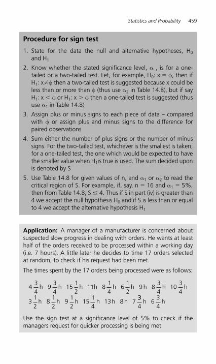
Statistics and Probability 459
Procedure for sign test
1. State for the data the null and alternative hypotheses, H 0 and H 1
2. Know whether the stated significance level, α , is for a one-tailed or a two-tailed test. Let, for example, H 0: x � φ, then if H1: x � φ then a two-tailed test is suggested because x could be less than or more than φ (thus use α 2 in Table 14.8 ), but if say H1: x φ or H 1: x φ then a one-tailed test is suggested (thus use α 1 in Table 14.8 )
3. Assign plus or minus signs to each piece of data – compared with φ or assign plus and minus signs to the difference for paired observations
4. Sum either the number of plus signs or the number of minus signs. For the two-tailed test, whichever is the smallest is taken; for a one-tailed test, the one which would be expected to have the smaller value when H 1is true is used. The sum decided upon is denoted by S
5. Use Table 14.8 for given values of n, and α 1 or α 2 to read the critical region of S. For example, if, say, n � 16 and α 1 � 5%, then from Table 14.8 , S � 4. Thus if S in part (iv) is greater than 4 we accept the null hypothesis H 0 and if S is less than or equal to 4 we accept the alternative hypothesis H 1
Application: A manager of a manufacturer is concerned about suspected slow progress in dealing with orders. He wants at least half of the orders received to be processed within a working day (i.e. 7 hours). A little later he decides to time 17 orders selected at random, to check if his request had been met.
The times spent by the 17 orders being processed were as follows:
434
934
1512
11 814
612
9 834
1034
312
812
912
1514
13 8 7
h h h h h h h h
h h h h
h
h h334
634
h h
Use the sign test at a significance level of 5% to check if the managers request for quicker processing is being met
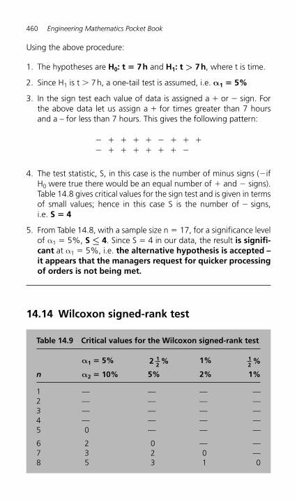
460 Engineering Mathematics Pocket Book
Using the above procedure:
1. The hypotheses are H0 : t � 7 h and H1 : t > 7 h , where t is time.
2. Since H 1 is t 7 h, a one-tail test is assumed, i.e. α 1 � 5%
3. In the sign test each value of data is assigned a � or � sign. For the above data let us assign a � for times greater than 7 hours and a – for less than 7 hours. This gives the following pattern:
� � � � � � � � �� � � � � � � �
4. The test statistic, S, in this case is the number of minus signs ( �ifH0 were true there would be an equal number of � and � signs). Table 14.8 gives critical values for the sign test and is given in terms of small values; hence in this case S is the number of � signs, i.e. S � 4
5. From Table 14.8 , with a sample size n � 17, for a significance level of α 1 � 5%, S ≤ 4 . Since S � 4 in our data, the result is signifi-cant at α 1 � 5%, i.e. the alternative hypothesis is accepted – it appears that the managers request for quicker processing of orders is not being met.
14.14 Wilcoxon signed-rank test
Table 14.9 Critical values for the Wilcoxon signed-rank test
α 1 � 5% 2 %12
1% 12 %
n α 2 � 10% 5% 2% 1%
1 — — — — 2 — — — — 3 — — — — 4 — — — — 5 0 — — —
6 2 0 — — 7 3 2 0 — 8 5 3 1 0
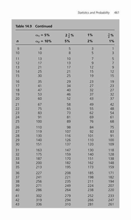
Statistics and Probability 461
Table 14.9 Continued
α 1 � 5% 2 %12
1% 12 %
n α 2 � 10% 5% 2% 1%
9 8 5 3 1 10 10 8 5 3
11 13 10 7 5 12 17 13 9 7 13 21 17 12 9 14 25 21 15 12 15 30 25 19 15
16 35 29 23 19 17 41 34 27 23 18 47 40 32 27 19 53 46 37 32 20 60 52 43 37
21 67 58 49 42 22 75 65 55 48 23 83 73 62 54 24 91 81 69 61 25 100 89 76 68
26 110 98 84 7527 119 107 92 8328 130 116 101 9129 140 126 110 10030 151 137 120 109
31 163 147 130 11832 175 159 140 12833 187 170 151 13834 200 182 162 14835 213 195 173 159
36 227 208 185 17137 241 221 198 18238 256 235 211 19439 271 249 224 20740 286 264 238 220
41 302 279 252 23342 319 294 266 24743 336 310 281 261
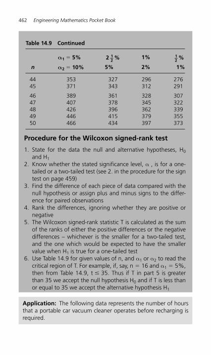
462 Engineering Mathematics Pocket Book
Table 14.9 Continued
α 1 � 5% 2 %12
1% 12 %
n α 2 � 10% 5% 2% 1%
44 353 327 296 27645 371 343 312 291
46 389 361 328 30747 407 378 345 32248 426 396 362 33949 446 415 379 35550 466 434 397 373
Procedure for the Wilcoxon signed-rank test
1. State for the data the null and alternative hypotheses, H 0 and H 1
2. Know whether the stated significance level, α , is for a one-tailed or a two-tailed test (see 2. in the procedure for the sign test on page 459)
3. Find the difference of each piece of data compared with the null hypothesis or assign plus and minus signs to the differ-ence for paired observations
4. Rank the differences, ignoring whether they are positive or negative
5. The Wilcoxon signed-rank statistic T is calculated as the sum of the ranks of either the positive differences or the negative differences – whichever is the smaller for a two-tailed test, and the one which would be expected to have the smaller value when H 1 is true for a one-tailed test
6. Use Table 14.9 for given values of n, and α 1 or α 2 to read the critical region of T. For example, if, say, n � 16 and α 1 � 5%, then from Table 14.9 , t � 35. Thus if T in part 5 is greater than 35 we accept the null hypothesis H 0 and if T is less than or equal to 35 we accept the alternative hypothesis H 1
Application: The following data represents the number of hours that a portable car vacuum cleaner operates before recharging is required.
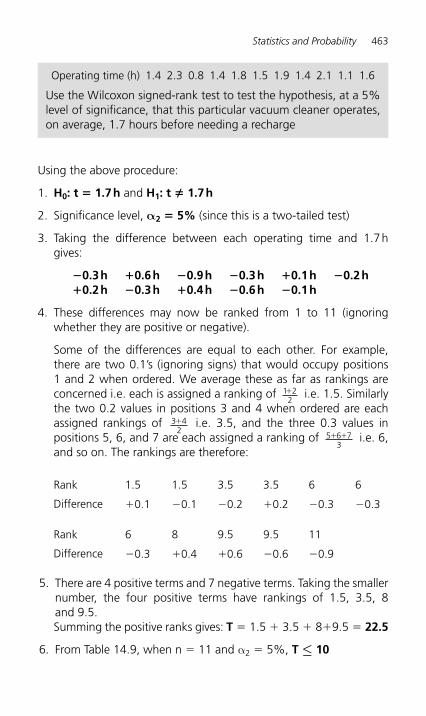
Statistics and Probability 463
Using the above procedure:
1. H0 : t � 1.7 h and H1 : t � 1.7 h
2. Significance level, α 2 � 5% (since this is a two-tailed test)
3. Taking the difference between each operating time and 1.7 h gives:
� 0.3 h � 0.6 h � 0.9 h � 0.3 h � 0.1 h � 0.2 h � 0.2 h � 0.3 h � 0.4 h � 0.6 h � 0.1 h
4. These differences may now be ranked from 1 to 11 (ignoring whether they are positive or negative).
Some of the differences are equal to each other. For example, there are two 0.1’s (ignoring signs) that would occupy positions 1 and 2 when ordered. We average these as far as rankings are concerned i.e. each is assigned a ranking of 1 2
2� i.e. 1.5. Similarly
the two 0.2 values in positions 3 and 4 when ordered are each assigned rankings of 3 4
2� i.e. 3.5, and the three 0.3 values in
positions 5, 6, and 7 are each assigned a ranking of 5 6 73
� � i.e. 6, and so on. The rankings are therefore:
Rank 1.5 1.5 3.5 3.5 6 6
Difference �0.1 �0.1 �0.2 �0.2 �0.3 � 0.3
Rank 6 8 9.5 9.5 11
Difference �0.3 �0.4 �0.6 �0.6 � 0.9
5. There are 4 positive terms and 7 negative terms. Taking the smaller number, the four positive terms have rankings of 1.5, 3.5, 8 and 9.5. Summing the positive ranks gives: T � 1.5 � 3.5 � 8�9.5 � 22.5
6. From Table 14.9 , when n � 11 and α 2 � 5%, T ≤ 10
Operating time (h) 1.4 2.3 0.8 1.4 1.8 1.5 1.9 1.4 2.1 1.1 1.6
Use the Wilcoxon signed-rank test to test the hypothesis, at a 5% level of significance, that this particular vacuum cleaner operates, on average, 1.7 hours before needing a recharge
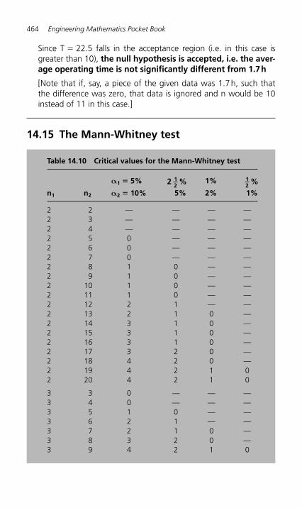
464 Engineering Mathematics Pocket Book
Since T � 22.5 falls in the acceptance region (i.e. in this case is greater than 10), the null hypothesis is accepted, i.e. the aver-age operating time is not significantly different from 1.7 h
[Note that if, say, a piece of the given data was 1.7 h, such that the difference was zero, that data is ignored and n would be 10 instead of 11 in this case.]
14.15 The Mann-Whitney test
Table 14.10 Critical values for the Mann-Whitney test
α 1 � 5% 2 %12
1% 12 %
n 1 n2 α 2 � 10% 5% 2% 1%
2 2 — — — — 2 3 — — — — 2 4 — — — — 2 5 0 — — — 2 6 0 — — — 2 7 0 — — — 2 8 1 0 — — 2 9 1 0 — — 2 10 1 0 — — 2 11 1 0 — — 2 12 2 1 — — 2 13 2 1 0 — 2 14 3 1 0 — 2 15 3 1 0 — 2 16 3 1 0 — 2 17 3 2 0 — 2 18 4 2 0 — 2 19 4 2 1 0 2 20 4 2 1 0
3 3 0 — — — 3 4 0 — — — 3 5 1 0 — — 3 6 2 1 — — 3 7 2 1 0 — 3 8 3 2 0 — 3 9 4 2 1 0
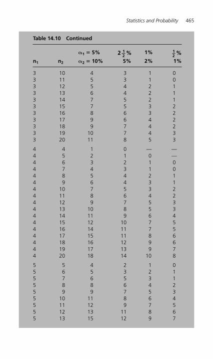
Statistics and Probability 465
Table 14.10 Continued
α 1 � 5% 2 %12
1% 12 %
n 1 n2 α 2 � 10% 5% 2% 1%
3 10 4 3 1 0 3 11 5 3 1 0 3 12 5 4 2 1 3 13 6 4 2 1 3 14 7 5 2 1 3 15 7 5 3 2 3 16 8 6 3 2 3 17 9 6 4 2 3 18 9 7 4 2 3 19 10 7 4 3 3 20 11 8 5 3
4 4 1 0 — — 4 5 2 1 0 — 4 6 3 2 1 0 4 7 4 3 1 0 4 8 5 4 2 1 4 9 6 4 3 1 4 10 7 5 3 2 4 11 8 6 4 2 4 12 9 7 5 3 4 13 10 8 5 3 4 14 11 9 6 4 4 15 12 10 7 5 4 16 14 11 7 54 17 15 11 8 64 18 16 12 9 64 19 17 13 9 74 20 18 14 10 8
5 5 4 2 1 05 6 5 3 2 15 7 6 5 3 15 8 8 6 4 25 9 9 7 5 35 10 11 8 6 45 11 12 9 7 55 12 13 11 8 65 13 15 12 9 7
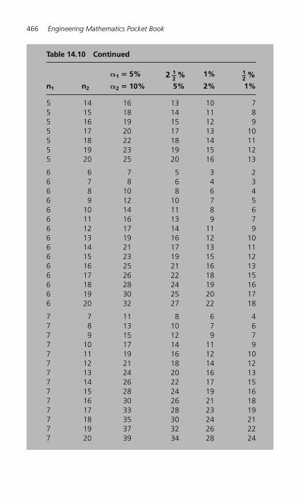
466 Engineering Mathematics Pocket Book
Table 14.10 Continued
α 1 � 5% 2 %12
1% 12 %
n 1 n2 α 2 � 10% 5% 2% 1%
5 14 16 13 10 75 15 18 14 11 85 16 19 15 12 95 17 20 17 13 105 18 22 18 14 115 19 23 19 15 125 20 25 20 16 13
6 6 7 5 3 26 7 8 6 4 36 8 10 8 6 46 9 12 10 7 56 10 14 11 8 66 11 16 13 9 76 12 17 14 11 96 13 19 16 12 106 14 21 17 13 116 15 23 19 15 126 16 25 21 16 136 17 26 22 18 156 18 28 24 19 166 19 30 25 20 176 20 32 27 22 18
7 7 11 8 6 47 8 13 10 7 67 9 15 12 9 77 10 17 14 11 97 11 19 16 12 107 12 21 18 14 127 13 24 20 16 137 14 26 22 17 157 15 28 24 19 167 16 30 26 21 187 17 33 28 23 197 18 35 30 24 217 19 37 32 26 227 20 39 34 28 24
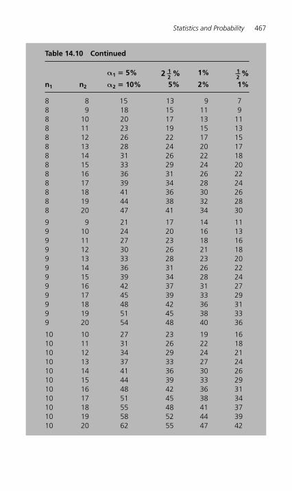
Statistics and Probability 467
Table 14.10 Continued
α 1 � 5% 2 %12
1% 12 %
n 1 n2 α 2 � 10% 5% 2% 1%
8 8 15 13 9 78 9 18 15 11 98 10 20 17 13 11 8 11 23 19 15 13 8 12 26 22 17 15 8 13 28 24 20 17 8 14 31 26 22 18 8 15 33 29 24 20 8 16 36 31 26 22 8 17 39 34 28 24 8 18 41 36 30 26 8 19 44 38 32 28 8 20 47 41 34 30
9 9 21 17 14 11 9 10 24 20 16 13 9 11 27 23 18 16 9 12 30 26 21 18 9 13 33 28 23 20 9 14 36 31 26 22 9 15 39 34 28 24 9 16 42 37 31 27 9 17 45 39 33 29 9 18 48 42 36 31 9 19 51 45 38 33 9 20 54 48 40 36
10 10 27 23 19 16 10 11 31 26 22 18 10 12 34 29 24 21 10 13 37 33 27 24 10 14 41 36 30 26 10 15 44 39 33 29 10 16 48 42 36 31 10 17 51 45 38 34 10 18 55 48 41 37 10 19 58 52 44 39 10 20 62 55 47 42
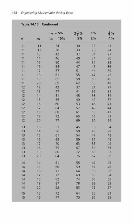
468 Engineering Mathematics Pocket Book
Table 14.10 Continued
α 1 � 5% 2 %12
1% 12 %
n 1 n2 α 2 � 10% 5% 2% 1%
11 11 34 30 25 21 11 12 38 33 28 24 11 13 42 37 31 27 11 14 46 40 34 30 11 15 50 44 37 33 11 16 54 47 41 36 11 17 57 51 44 39 11 18 61 55 47 42 11 19 65 58 50 45 11 20 69 62 53 48 12 12 42 37 31 27 12 13 47 41 35 3112 14 51 45 38 3412 15 55 49 42 3712 16 60 53 46 4112 17 64 57 49 4412 18 68 61 53 4712 19 72 65 56 5112 20 77 69 60 54
13 13 51 45 39 3413 14 56 50 43 3813 15 61 54 47 4213 16 65 59 51 4513 17 70 63 55 4913 18 75 67 59 5313 19 80 72 63 5713 20 84 76 67 60
14 14 61 55 47 4214 15 66 59 51 4614 16 71 64 56 5014 17 77 69 60 5414 18 82 74 65 5814 19 87 78 69 6314 20 92 83 73 67
15 15 72 64 56 5115 16 77 70 61 55
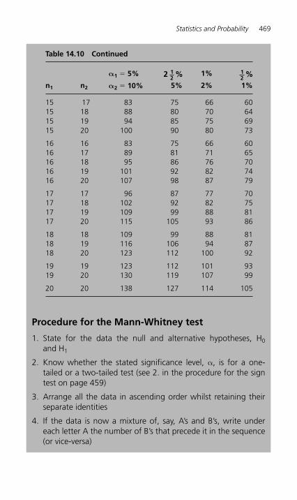
Statistics and Probability 469
Table 14.10 Continued
α 1 � 5% 2 %12
1% 12 %
n 1 n2 α 2 � 10% 5% 2% 1%
15 17 83 75 66 6015 18 88 80 70 6415 19 94 85 75 6915 20 100 90 80 73
16 16 83 75 66 6016 17 89 81 71 6516 18 95 86 76 7016 19 101 92 82 7416 20 107 98 87 79
17 17 96 87 77 7017 18 102 92 82 7517 19 109 99 88 8117 20 115 105 93 86
18 18 109 99 88 8118 19 116 106 94 8718 20 123 112 100 92
19 19 123 112 101 9319 20 130 119 107 99
20 20 138 127 114 105
Procedure for the Mann-Whitney test
1. State for the data the null and alternative hypotheses, H 0 and H 1
2. Know whether the stated significance level, α, is for a one-tailed or a two-tailed test (see 2. in the procedure for the sign test on page 459)
3. Arrange all the data in ascending order whilst retaining their separate identities
4. If the data is now a mixture of, say, A’s and B’s, write under each letter A the number of B’s that precede it in the sequence (or vice-versa)
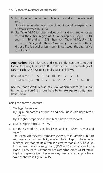
470 Engineering Mathematics Pocket Book
5. Add together the numbers obtained from 4 and denote total by U. U is defined as whichever type of count would be expected to be smallest when H 1 is true
6. Use Table 14.10 for given values of n 1 and n 2 , and α 1 or α 2 to read the critical region of U. For example, if, say, n 1 � 10 and n 2 � 16 and α 2 � 5%, then from Table 14.10, U � 42. If U in part 5 is greater than 42 we accept the null hypothesis H0, and if U is equal or less than 42, we accept the alternative hypothesis H 1
Application: 10 British cars and 8 non-British cars are compared for faults during their first 10000 miles of use. The percentage of cars of each type developing faults were as follows:
Non-British cars, P 5 8 14 10 15 7 12 4
British cars, Q 18 9 25 6 21 20 28 11 16 34
Use the Mann-Whitney test, at a level of significance of 1%, to test whether non-British cars have better average reliability than British models
Using the above procedure:
1. The hypotheses are: H 0 : Equal proportions of British and non-British cars have break-
downs H 1 : A higher proportion of British cars have breakdowns
2. Level of significance α 1 � 1%
3. Let the sizes of the samples be n P and n Q, where n P � 8 and nQ � 10 The Mann-Whitney test compares every item in sample P in turn with every item in sample Q, a record being kept of the number of times, say, that the item from P is greater than Q, or vice-versa. In this case there are n P nQ , i.e. (8)(10) � 80 comparisons to be made. All the data is arranged into ascending order whilst retain-ing their separate identities – an easy way is to arrange a linear scale as shown in Figure 14.15 .
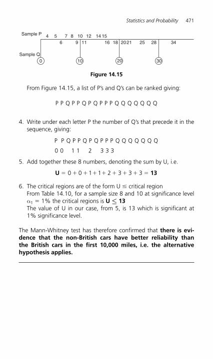
Statistics and Probability 471
From Figure 14.15 , a list of P’s and Q’s can be ranked giving:
P P Q P P Q P Q P P P Q Q Q Q Q Q Q
4. Write under each letter P the number of Q’s that precede it in the sequence, giving:
P P Q P P Q P Q P P P Q Q Q Q Q Q Q
0 1 0 1 2 3 3 3 5. Add together these 8 numbers, denoting the sum by U, i.e.
U 13� � � � � � � � �0 0 1 1 2 3 3 3
6. The critical regions are of the form U � critical region From Table 14.10 , for a sample size 8 and 10 at significance level α 1 � 1% the critical regions is U ≤ 13 The value of U in our case, from 5, is 13 which is significant at 1% significance level.
The Mann-Whitney test has therefore confirmed that there is evi-dence that the non-British cars have better reliability than the British cars in the first 10,000 miles, i.e. the alternative hypothesis applies.
Sample P
Sample Q
4 59 11 16 18 2021 25 28 346
0 10 20 30
7 8 10 12 14 15
Figure 14.15
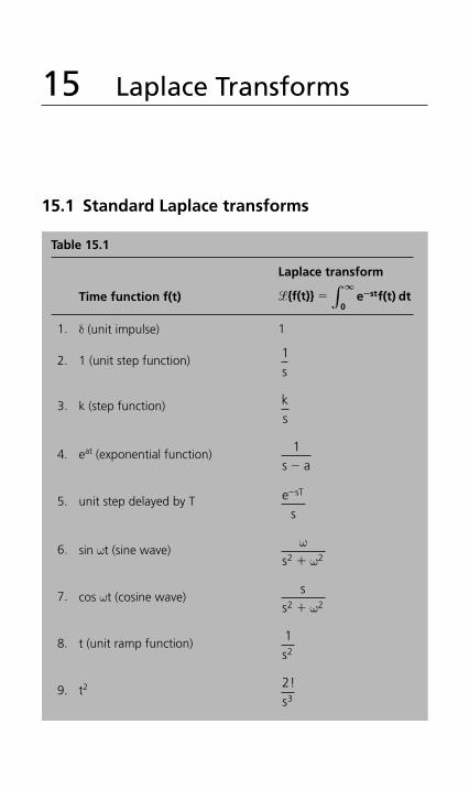
15 Laplace Transforms
15.1 Standard Laplace transforms
Table 15.1
Time function f(t)
Laplace transform
� { f(t) } � e f(t) dtst
0
�∞
∫
1. δ (unit impulse) 1
2. 1 (unit step function)
1s
3. k (step function)
ks
4. eat (exponential function)
1s a�
5. unit step delayed by T
es
sT�
6. sin ω t (sine wave)
ωωs2 2�
7. cos ω t (cosine wave)
ss2 2� ω
8. t (unit ramp function)
12s
9. t2
23
!s
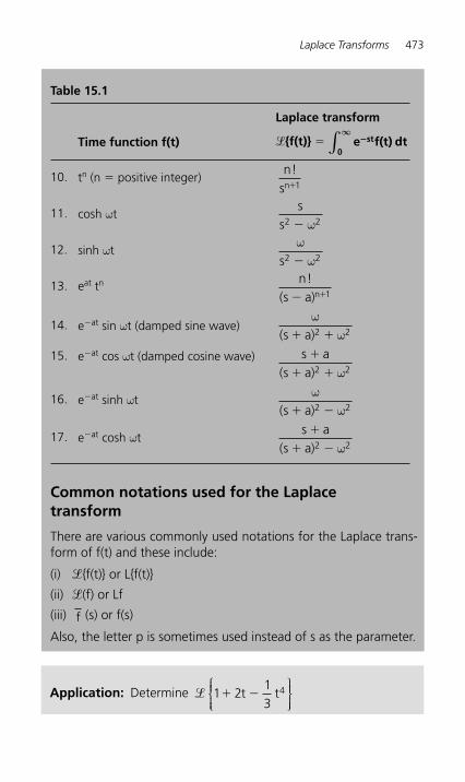
Laplace Transforms 473
Table 15.1
Time function f(t)
Laplace transform
� { f(t) } � e f(t) dtst
0
�∞
∫10. t n (n � positive integer)
n!sn�1
11. cosh ω t
ss2 2� ω
12. sinh ω t
ωωs2 2�
13. eat t n
ns a n
!( )� �1
14. e � at sin ω t (damped sine wave)
ωω( )s � �a 2 2
15. e � at cos ω t (damped cosine wave)
s �
� �
as a( )2 2ω
16. e � at sinh ω t
ωω( )s a� �2 2
17. e � at cosh ω t
s as a
�
� �( )2 2ω
Common notations used for the Laplace transform
There are various commonly used notations for the Laplace trans-form of f(t) and these include:
(i) � { f(t) } or L { f(t) }
(ii) � (f) or Lf
(iii) f (s) or f(s)
Also, the letter p is sometimes used instead of s as the parameter.
Application: Determine � 1 213
4� �t t⎧⎨⎪⎪⎩⎪⎪
⎫⎬⎪⎪⎭⎪⎪
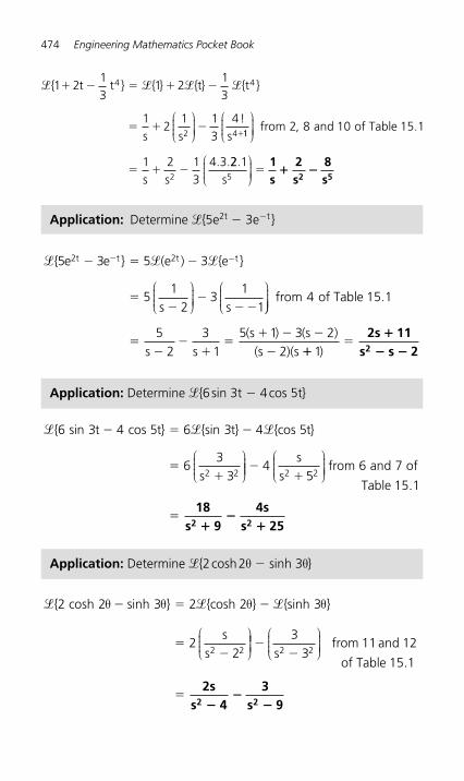
474 Engineering Mathematics Pocket Book
� � � �{ t t } { } {t} {t }
s s s
1 213
1 213
12
1 13
4
4 4
2 4
� � � � �
� � ��
⎛⎝⎜⎜⎜
⎞⎠⎟⎟⎟⎟
!11
2
2 8 10 15 1
1 2 13
4 3
⎛⎝⎜⎜⎜
⎞⎠⎟⎟⎟⎟ from , and of Table
s s
.
. .� � �
22 15
.s
⎛⎝⎜⎜⎜
⎞⎠⎟⎟⎟⎟ �
1s
2s
8s2 5
� �
Application: Determine � { 5e 2t � 3e � t }
� � �{ e e } (e ) {e }
s s
t t 2t t5 3 5 3
51
23
11
2 � � �
��
�� �
� −
⎛⎝⎜⎜⎜
⎞⎠⎟⎟⎟⎟
⎛⎝⎜⎜⎜
⎞⎠⎠⎟⎟⎟⎟ from of Table
s s(s ) (s 2)
(s )(s
4 15 1
52
31
5 1 32
.
��
��
�� � �
� ���
1)2s 11
s s 22
�
� �
Application: Determine � { 6 sin 3t � 4 cos 5t }
� � �{ sin t cos t} {sin t} {cos t}
s
6 3 4 5 6 3 4 5
63
32 2
� � �
��
⎛⎝⎜⎜⎜
⎞⎠⎟⎟⎟⎟⎟
⎛⎝⎜⎜⎜
⎞⎠⎟⎟⎟⎟�
�4
56 7
2 2
ss
from and of
Table 15 1.
�18
s 94s
s 252 2��
�
Application: Determine � { 2 cosh 2 θ � sinh 3 θ }
� � �{2 cosh sinh } {cosh } {sinh }
s
2 3 2 2 3
222 2
θ � � �
��
θ θ θ
s
⎛⎝⎜⎜⎜
⎞⎠⎟⎟⎟⎟⎟
⎛⎝⎜⎜⎜
⎞⎠⎟⎟⎟⎟�
�
33
11 122 2s
from and
of Table 15 1.
�2s
s 43
s 92 2��
�
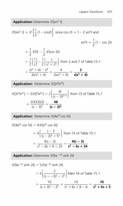
Laplace Transforms 475
� �{sin t} cos since cos 2t sin t2 212
1 2 1 2� � � �( t⎧⎨⎪⎪⎩⎪⎪
⎫⎬⎪⎪⎭⎪⎪
and
sin t ( cos t)
{ } {cos t}
s
2 12
1 2
12
112
2
12
1
� �
� �
�
� �
⎛⎝⎜⎜⎜
⎞⎠⎟⎟⎟⎟⎟
⎛⎝⎜⎜⎜
⎞⎠⎟⎟⎟⎟�
�
�� �
12 2
2 7 15 1
4
2 2
2
ss
from and of Table
s s
.
( ) 22
2 22 44
2 4s s s s( ) ( )��
��
2s(s 4)2 �
Application: Determine � { sin 2 t }
Application: Determine � { 2t 4 e 3t }
� �{ t e } {t e }!
(s from of Tabt t2 2 2
43
134 3 4 34 1
� �� �)
⎛
⎝⎜⎜⎜⎜
⎞
⎠⎟⎟⎟⎟ lle
s
15 1
2 4 3 23 5
.
( )( )( )( )
��
�48
(s 3)5�
Application: Determine � { 4e 3t cos 5t }
� �{ e cos t} {e cos t}
s(s )
from
t t4 5 4 5
43
3 5
3 3
2 2
�
��
� �
⎛
⎝⎜⎜⎜⎜
⎞
⎠⎟⎟⎟⎟ of Table
(ss s
15 15 1
4 36 9 252
.
)�
�
� ��
+4(s 3)
s 6s 342
�
� �
Application: Determine � { 5e � 3t sinh 2t }
� �{ e sinh t} {e sinh t}
(sfr
t t5 2 5 2
523 2
3 3
2 2
� ��
�� � �)
⎛
⎝⎜⎜⎜⎜
⎞
⎠⎟⎟⎟⎟ oom of Table
(s ) s s
16 15 1
103 2
106 9 42 2 2
.
�� �
�� � �
�10
s 6s 52 � �
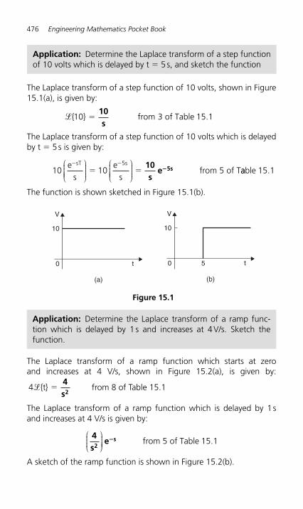
476 Engineering Mathematics Pocket Book
The Laplace transform of a step function of 10 volts, shown in Figure 15.1(a) , is given by:
�{ } from of Table 10 3 15 1�10s
.
The Laplace transform of a step function of 10 volts which is delayed by t � 5 s is given by:
10 10 55e
se
sfrom of T
sT s� �
� �⎛
⎝⎜⎜⎜⎜
⎞
⎠⎟⎟⎟⎟
⎛
⎝⎜⎜⎜⎜
⎞
⎠⎟⎟⎟⎟
10s
e 5s� aable 15 1.
The function is shown sketched in Figure 15.1(b) .
Application: Determine the Laplace transform of a step function of 10 volts which is delayed by t � 5 s, and sketch the function
V
10
(a)
t0
(b)
V
10
t0 5
Figure 15.1
The Laplace transform of a ramp function which starts at zero and increases at 4 V/s, shown in Figure 15.2(a) , is given by:
4�{t} �4s2
from 8 of Table 15.1
The Laplace transform of a ramp function which is delayed by 1 s and increases at 4 V/s is given by:
4s
e2
s⎛⎝⎜⎜⎜
⎞⎠⎟⎟⎟⎟
� from of Table 5 15 1.
A sketch of the ramp function is shown in Figure 15.2(b) .
Application: Determine the Laplace transform of a ramp func-tion which is delayed by 1 s and increases at 4 V/s. Sketch the function.
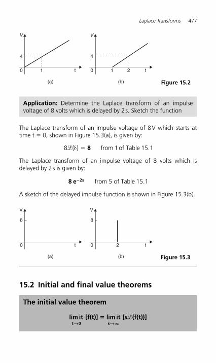
Laplace Transforms 477
V
4
(a)
t0 1
V
4
(b)
t0 1 2
Figure 15.2
The Laplace transform of an impulse voltage of 8 V which starts at time t � 0, shown in Figure 15.3(a) , is given by:
8 1 15 1�{ } from of Table δ � 8 .
The Laplace transform of an impulse voltage of 8 volts which is delayed by 2 s is given by:
8 e 2s� from of Table 5 15 1.
A sketch of the delayed impulse function is shown in Figure 15.3(b) .
Application: Determine the Laplace transform of an impulse voltage of 8 volts which is delayed by 2 s. Sketch the function
Figure 15.3
V
8
(a)
t0
(b)
V
8
t0 2
15.2 Initial and final value theorems
The initial value theorem
lim it [f(t)] lim it [s {f(t)}]t 0 s→ →∞
� �
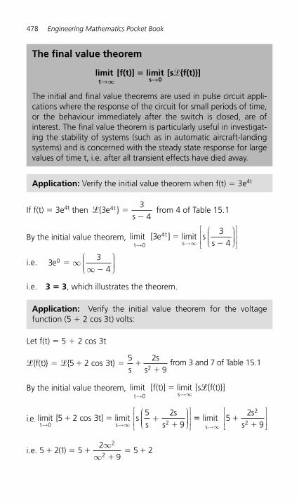
478 Engineering Mathematics Pocket Book
The final value theorem
limit [f(t)] limit [s {f(t)}]t s 0→∞ →
� �
The initial and final value theorems are used in pulse circuit appli-cations where the response of the circuit for small periods of time, or the behaviour immediately after the switch is closed, are of interest. The final value theorem is particularly useful in investigat-ing the stability of systems (such as in automatic aircraft-landing systems) and is concerned with the steady state response for large values of time t, i.e. after all transient effects have died away.
Application: Verify the initial value theorem when f(t) � 3e 4t
If f(t) � 3e 4t then �{ e }s
t33
44 �
� from 4 of Table 15.1
By the initial value theorem, limit [ e ] limit sst
t
s→ →∞0
433
4�
�
⎛⎝⎜⎜⎜
⎞⎠⎟⎟⎟⎟
⎡
⎣⎢⎢
⎤
⎦⎥⎥
i.e. 33
40e �
�∞
∞
⎛⎝⎜⎜⎜
⎞⎠⎟⎟⎟⎟
i.e. 3 � 3 , which illustrates the theorem.
Application: Verify the initial value theorem for the voltage function (5 � 2 cos 3t) volts:
Let f(t) � 5 � 2 cos 3t
� �{f(t)} { cos t}s
ss
� � � ��
5 2 35 2
92 from 3 and 7 of Table 15.1
By the initial value theorem, limit [f(t)] limit [s {f(t)}]t s→ →∞0
� �
i.e. limit [ cos t] limits sst
ss
→+
⎛⎝⎜⎜⎜
⎞⎠⎟⎟⎟⎟
⎡
⎣⎢⎢
⎤
⎦⎥⎥0 2
5 2 35 2
9� �
�→∞�� �
�limit
sss→∞
52
9
2
2
⎡
⎣⎢⎢
⎤
⎦⎥⎥
i.e. 5 2 1 52
95 2
2
2� � �
�� �( )
∞∞
Laplace Transforms 479
Application: Verify the final value theorem when f(t) � 3e � 4t
limit [ e ] limit ss
t
t s→∞ →
⎛⎝⎜⎜⎜
⎞⎠⎟⎟⎟⎟
⎡
⎣⎢⎢
⎤
⎦⎥⎥3
34
4
0
� ��
i.e. 3 0
30 4
e ( )�� ��
⎛⎝⎜⎜⎜
⎞⎠⎟⎟⎟⎟
i.e. 0 � 0, which illustrates the theorem.
i.e. 7 � 7 , which verifies the theorem in this case.
The initial value of the voltage is thus 7 V
Application: Verify the final value theorem for the function (2 � 3e � 2t sin 4t) cm, which represents the displacement of a particle
Let f(t) � 2 � 3e � 2t sin 4t
� �{f(t)} {2 e sin t}s (s
2s
1
� � � �� � �
� �
�3 42
342 4
22 2
t
)
⎛
⎝⎜⎜⎜⎜
⎞
⎠⎟⎟⎟⎟
22(s
from and of Table � �2 16
3 14 15 12)
.
By the final value theorem, limit [f(t)] limit [s {f(t)}]t s→∞ →
�0
�
i.e. limit [ e sin t] limit s
s (s )t
t
→∞2 3 4
2 122 16
2
0 2� � �
� ��
s→
⎛
⎝⎜⎜⎜⎜
⎞
⎠⎟⎟⎟⎟⎟
⎡
⎣⎢⎢⎢
⎤
⎦⎥⎥⎥
� �
� �limit
s(s )s→0 2
2122 16
⎡
⎣⎢⎢
⎤
⎦⎥⎥
i.e. 2 � 0 � 2 � 0
i.e. 2 � 2 , which verifies the theorem in this case.
The final value of the displacement is thus 2 cm.
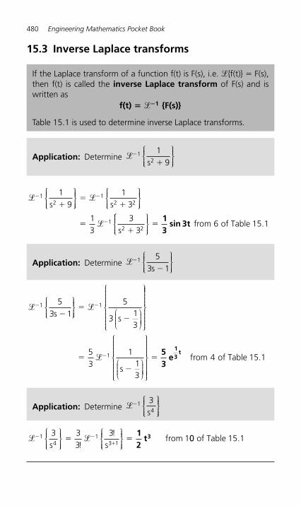
480 Engineering Mathematics Pocket Book
� �
�
� �
�
��
�
��
12
12 2
12 2
19
13
13
33
s s
s
⎧⎨⎪⎪⎩⎪⎪
⎫⎬⎪⎪⎭⎪⎪
⎧⎨⎪⎪⎩⎪⎪
⎫⎬⎪⎪⎭⎪⎪
⎧⎧⎨⎪⎪⎩⎪⎪
⎫⎬⎪⎪⎭⎪⎪
�13
sin 3t from of Table 6 15 1.
If the Laplace transform of a function f(t) is F(s), i.e. � { f(t) } � F(s), then f(t) is called the inverse Laplace transform of F(s) and is written as
f(t) {F(s)}1� ��
Table 15.1 is used to determine inverse Laplace transforms .
Application: Determine ��
�1
2
19s
⎧⎨⎪⎪⎩⎪⎪
⎫⎬⎪⎪⎭⎪⎪
Application: Determine ��
�1 5
3 1s
⎧⎨⎪⎪⎩⎪⎪
⎫⎬⎪⎪⎭⎪⎪
� �� �
��
�
1 153 1
5
313
s s
⎧⎨⎪⎪⎩⎪⎪
⎫⎬⎪⎪⎭⎪⎪ ⎛
⎝⎜⎜⎜
⎞⎠⎟⎟⎟⎟
⎧
⎨
⎪⎪⎪⎪⎪
⎩
⎪⎪⎪⎪⎪
⎫
⎬
⎪⎪⎪⎪⎪⎪
⎭
⎪⎪⎪⎪⎪
⎛⎝⎜⎜⎜
⎞⎠⎟⎟⎟⎟
⎧
⎨
⎪⎪⎪⎪⎪
⎩
⎪⎪⎪⎪⎪
⎫
⎬
⎪⎪⎪⎪⎪
⎭
⎪⎪⎪�
�
�53
113
1�
s ⎪⎪⎪
�53
e13
tfrom of Table 4 15 1.
Application: Determine ��14
3s
⎧⎨⎪⎪⎩⎪⎪
⎫⎬⎪⎪⎭⎪⎪
� �� ��
� �14
13 1
3 33
31
s !!
sfrom
⎧⎨⎪⎪⎩⎪⎪
⎫⎬⎪⎪⎭⎪⎪
⎧⎨⎪⎪⎩⎪⎪
⎫⎬⎪⎪⎭⎪⎪
12
t3 00 15 1 of Table .
15.3 Inverse Laplace transforms
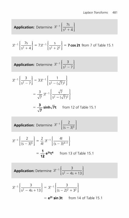
Laplace Transforms 481
Application: Determine ��
�1
2
74
ss
⎧⎨⎪⎪⎩⎪⎪
⎫⎬⎪⎪⎭⎪⎪
� �� �
��
��1
21
2 2
74 2
ss
7s
sf
⎧⎨⎪⎪⎩⎪⎪
⎫⎬⎪⎪⎭⎪⎪
⎧⎨⎪⎪⎩⎪⎪
⎫⎬⎪⎪⎭⎪⎪
7 cos 2t rrom of Table 7 15 1.
Application: Determine ��
�1
2
37s
⎧⎨⎪⎪⎩⎪⎪
⎫⎬⎪⎪⎭⎪⎪
� �
�
� �
�
��
�
�
12
12 2
12
37
1
7
3
7
7
s3
s
s
⎧⎨⎪⎪⎩⎪⎪
⎫⎬⎪⎪⎭⎪⎪
⎧⎨⎪⎪⎩⎪⎪
⎫⎬⎪⎪⎭⎪⎪( )
��
�
( )
.
7
12 15 1
2
⎧⎨⎪⎪
⎩⎪⎪
⎫⎬⎪⎪
⎭⎪⎪
37
sinh 7t from of Table
Application: Determine ��
�1
5
23( )s
⎧⎨⎪⎪⎩⎪⎪
⎫⎬⎪⎪⎭⎪⎪
� �� ���
��
�
15
14 1
23
24
43( ) ( )s !!
s
⎧⎨⎪⎪⎩⎪⎪
⎫⎬⎪⎪⎭⎪⎪
⎧⎨⎪⎪⎩⎪⎪
⎫⎬⎪⎪⎭⎪⎪
1122
e t3t 4 from 13 of Table 15.1
Application: Determine ��
� �1
2
34 13s s
⎧⎨⎪⎪⎩⎪⎪
⎫⎬⎪⎪⎭⎪⎪
� �� �
� ��
� �
�
12
12 2
34 13
32 3s s s
⎧⎨⎪⎪⎩⎪⎪
⎫⎬⎪⎪⎭⎪⎪
⎧⎨⎪⎪⎩⎪⎪
⎫⎬⎪⎪⎭⎪⎪( )
e2t ssin 3t from of Table 14 15 1.

482 Engineering Mathematics Pocket Book
� �� ��
� ��
�
� �1
21
2 2
4 34 5
4 32 3
ss s
ss
⎧⎨⎪⎪⎩⎪⎪
⎫⎬⎪⎪⎭⎪⎪
⎧⎨⎪⎪⎩⎪⎪
⎫⎬⎪⎪⎭⎪( ) ⎪⎪
⎧⎨⎪⎪⎩⎪⎪
⎫⎬⎪⎪⎭⎪⎪
⎧⎨
�� �
� �
��
� �
�
�
�
�
12 2
12 2
4 2 52 3
4 22 3
( )( )
( )
ss
s(s )
⎪⎪⎪⎩⎪⎪
⎫⎬⎪⎪⎭⎪⎪
⎧⎨⎪⎪⎩⎪⎪
⎫⎬⎪⎪⎭⎪⎪
�� �
� �
�
�
�
�
12 2
2 1
52 3
4 3
( )s
e cosh tt
553
3
2 32 2
( )
( )s � �
⎧
⎨
⎪⎪⎪⎪⎪
⎩⎪⎪⎪⎪⎪
⎫
⎬
⎪⎪⎪⎪⎪
⎭⎪⎪⎪⎪⎪
from of Table 17 15 1.
� 4e cosh 3t53
e2t � 22t sinh 3t
from of T16 aable 15 1.
Inverse Laplace transforms using partial fractions
Application: Determine �� �
� �1
2
4 52
ss s
⎧⎨⎪⎪⎩⎪⎪
⎫⎬⎪⎪⎭⎪⎪
Let
4 52
4 52 1 2 1
1 222
ss s
s(s )(s )
A(s )
B(s )
A(s ) B(s )(s )
�
� �
�
� � ��
�
� � �
�≡ ≡ ≡
((s )�1
Hence, 4s � 5 � A(s � 1) � B(s � 2)
When s � 2, 3 � 3A, from which, A � 1
When s � � 1, � 9 � � 3B, from which, B � 3
Hence
� � �� � ��
� � ��
��1
21 14 5
21
23
1s
s s s s
⎧⎨⎪⎪⎩⎪⎪
⎫⎬⎪⎪⎭⎪⎪
⎧⎨⎪⎪⎩⎪⎪
⎫⎬⎪⎪⎭⎪⎪
≡11
23
11
s s��
��
⎧⎨⎪⎪⎩⎪⎪
⎫⎬⎪⎪⎭⎪⎪
⎧⎨⎪⎪⎩⎪⎪
⎫⎬⎪⎪⎭⎪⎪
�
� e 3e2t t� � from 4 of Table 15.1
Application: Determine �� �
� �1
2
4 34 5
ss s
⎧⎨⎪⎪⎩⎪⎪
⎫⎬⎪⎪⎭⎪⎪
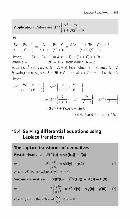
Laplace Transforms 483
Application: Determine �� � �
� �1
2
2
5 8 13 1
s ss )(s )(
⎧⎨⎪⎪⎩⎪⎪
⎫⎬⎪⎪⎭⎪⎪
Let
5 8 13 1 3 1
1 32
2 2
2s s(s )(s )
As
Bs C(s )
A(s ) (Bs C)(s )(s
� �
� � ��
�
�
� � � �
�≡ ≡
33 12)(s )� Hence, 5s 2 � 8s � 1 � A(s 2 � 1) � (Bs � C)(s � 3) When s � � 3, 20 � 10A, from which, A � 2 Equating s 2 terms gives: 5 � A � B, from which, B � 3, since A � 2 Equating s terms gives: 8 � 3B � C, from which, C � �1, since B � 3
Hence
� �� �� �
� � ��
�
�1
2
21
2
5 8 13 1
23
3 11
s s(s )(s ) s
ss
⎧⎨⎪⎪⎩⎪⎪
⎫⎬⎪⎪⎭⎪⎪
⎧⎨⎪⎪⎩
≡⎪⎪⎪
⎫⎬⎪⎪⎭⎪⎪
≡ � � �� � �
��
��
�1 1
21
2
23
31
11s
⎧⎨⎪⎪⎩⎪⎪
⎫⎬⎪⎪⎭⎪⎪
⎧⎨⎪⎪⎩⎪⎪
⎫⎬⎪⎪⎭⎪⎪
⎧⎨⎪s
s s⎪⎪⎩⎪⎪
⎫⎬⎪⎪⎭⎪⎪
� 2e 3cos t sin t3t� � �
froom , and of Table 4 7 6 15 1.
15.4 Solving differential equations using Laplace transforms
The Laplace transforms of derivatives
First derivatives: � { f � (t) } � s � { f(t) } � f(0)
or � �dydx
s {y} y(0)⎧⎨⎪⎪⎩⎪⎪
⎫⎬⎪⎪⎭⎪⎪
� � (1)
where y(0) is the value of y at x � 0
Second derivative: � { f (t) } � s 2 � { f(t) } � sf(0) � f � (0)
or � �d ydx
s {y} s y(0) y (0)2
22
⎧⎨⎪⎪⎩⎪⎪
⎫⎬⎪⎪⎭⎪⎪
� � � � (2)
where y � ( 0) is the value of dydx
at x � 0
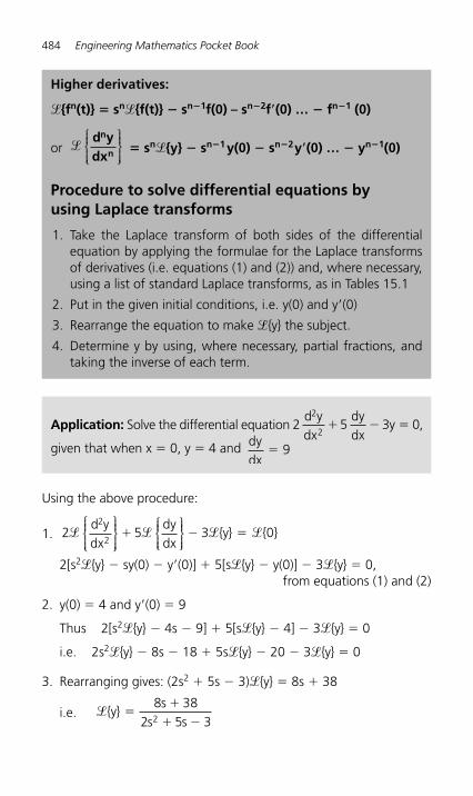
484 Engineering Mathematics Pocket Book
Using the above procedure:
1. 2 5 3 02
2� � � �
d ydx
dydx
{y} { }⎧⎨⎪⎪⎩⎪⎪
⎫⎬⎪⎪⎭⎪⎪
⎧⎨⎪⎪⎩⎪⎪
⎫⎬⎪⎪⎭⎪⎪
� � �
2[s 2 � { y } � sy(0) � y � (0)] � 5[s � { y } � y(0)] � 3 � { y } � 0,from equations (1) and (2)
2. y(0) � 4 and y � (0) � 9
Thus 2[s 2 � { y } � 4s � 9] � 5[s � { y} � 4] � 3 � { y } � 0
i.e. 2s 2 � { y } � 8s � 18 � 5s � { y} � 20 � 3 � { y } � 0
3. Rearranging gives: (2s 2 � 5s � 3) � { y } � 8s � 38
i.e. �{y}s
s s�
�
� �
8 382 5 32
Higher derivatives:
� { f n (t) } � s n � { f(t) } � s n � 1f (0) – s n � 2 f � (0) … � f n � 1 (0)
or �d ydx
n
n
⎧⎨⎪⎪⎩⎪⎪
⎫⎬⎪⎪⎭⎪⎪
� s n � { y } � s n � 1 y(0) � s n � 2 y � (0) … � y n � 1 (0)
Procedure to solve differential equations by using Laplace transforms
1. Take the Laplace transform of both sides of the differential equation by applying the formulae for the Laplace transforms of derivatives (i.e. equations (1) and (2)) and, where necessary, using a list of standard Laplace transforms, as in Tables 15.1
2. Put in the given initial conditions, i.e. y(0) and y � (0)
3. Rearrange the equation to make � { y } the s ubject.
4. Determine y by using, where necessary, partial fractions, and taking the inverse of each term.
Application: Solve the differential equation 2 5 3 02
2
d ydx
dydx
y� � � ,
given that when x � 0, y � 4 and dydx
� 9
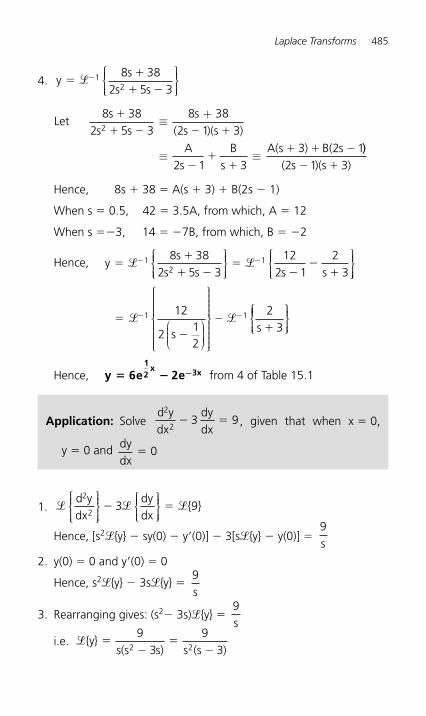
Laplace Transforms 485
4. ys
s s�
�
� ��� 1
2
8 382 5 3
⎧⎨⎪⎪⎩⎪⎪
⎫⎬⎪⎪⎭⎪⎪
Let8 38
2 5 38 38
2 1 3
2 1 33 2 1
2
ss s
ss )(s )
As
Bs
A(s ) B( s
�
� � � �
��
�
� � �
≡
≡ ≡
+(
))( s )(s )2 1 3� �
Hence, 8s � 38 � A(s � 3) � B(2s � 1)
When s � 0.5, 42 � 3.5A, from which, A � 12
When s ��3, 14 � � 7B, from which, B � � 2
Hence, ys
s s s s�
�
� ��
��
�� �� �1
218 38
2 5 312
2 12
3
⎧⎨⎪⎪⎩⎪⎪
⎫⎬⎪⎪⎭⎪⎪
⎧⎨⎪⎪⎩⎪⎪
⎫⎬⎪⎪⎭⎭⎪⎪
�
�
��
� �� �1 112
212
23s s⎛
⎝⎜⎜⎜
⎞⎠⎟⎟⎟⎟
⎧
⎨
⎪⎪⎪⎪⎪
⎩
⎪⎪⎪⎪⎪
⎫
⎬
⎪⎪⎪⎪⎪
⎭
⎪⎪⎪⎪⎪
⎧⎨⎪⎪⎪⎩⎪⎪
⎫⎬⎪⎪⎭⎪⎪
Hence, y 6e 2e12
x 3x� � − from 4 of Table 15.1
Application: Solve d ydx
dydx
2
23 9� � , given that when x � 0,
y � 0 and dydx
� 0
1. � � �d ydx
dydx
{ }2
23 9
⎧⎨⎪⎪⎩⎪⎪
⎫⎬⎪⎪⎭⎪⎪
⎧⎨⎪⎪⎩⎪⎪
⎫⎬⎪⎪⎭⎪⎪
� �
Hence, [s 2 � { y } � sy(0) � y � (0)] � 3[s � { y} � y(0)] � 9s
2. y(0) � 0 and y � (0) � 0
Hence, s 2 � { y } � 3s� { y} � 9s
3. Rearranging gives: (s 2 � 3s) � { y } � 9s
i.e. �{y}s(s s) s (s )
��
��
93
932 2
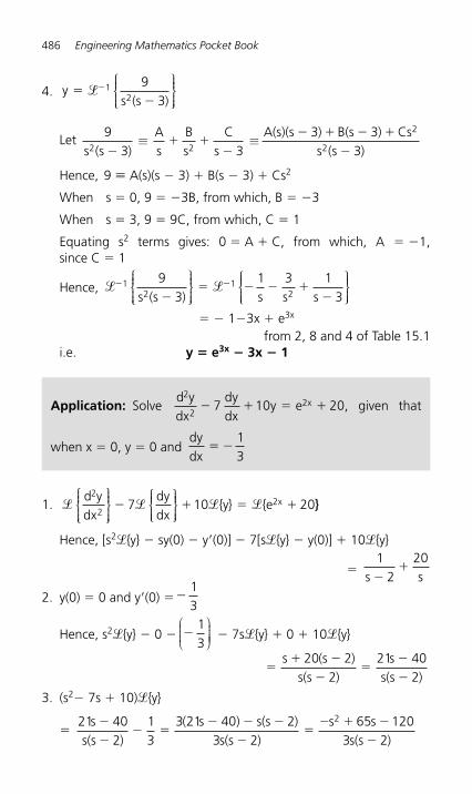
486 Engineering Mathematics Pocket Book
4. ys (s )
��
�� 12
93
⎧⎨⎪⎪⎩⎪⎪
⎫⎬⎪⎪⎭⎪⎪
Let 9
3 33 3
32 2
2
2s (s )As
Bs
Cs
A(s)(s ) B(s ) Css (s )�
� ��
� � � �
�≡ ≡
Hence, 9 � A(s)(s � 3) � B(s � 3) � Cs2
When s � 0, 9 � � 3B, from which, B � � 3
When s � 3, 9 � 9C, from which, C � 1
Equating s 2 terms gives: 0 � A � C, from which, A � � 1,since C � 1
Hence, � �� �
�� � � �
�1
21
2
93
1 3 13s (s s s s)
⎧⎨⎪⎪⎩⎪⎪
⎫⎬⎪⎪⎭⎪⎪
⎧⎨⎪⎪⎩⎪⎪
⎫⎬⎪⎪⎭⎪⎪
� � 1 � 3x � e 3x from 2, 8 and 4 of Table 15.1
i.e. y � e 3x � 3x � 1
Application: Solve d ydx
dydx
y e x2
227 10 20� � � � , given that
when x � 0, y � 0 and dydx
� �13
1. � � � �d ydx
7dydx
{y} {e x2
2210 20
⎧⎨⎪⎪⎩⎪⎪
⎫⎬⎪⎪⎭⎪⎪
⎧⎨⎪⎪⎩⎪⎪
⎫⎬⎪⎪⎭⎪⎪
� � � � }}
Hence, [s 2 � { y } � sy(0) � y � (0)] � 7[s � { y } � y(0)] � 10 � { y }
�
12
20s s�
�
2. y(0) � 0 and y � (0) � �13
Hence, s 2 � { y } � 0 � �13
⎛⎝⎜⎜⎜
⎞⎠⎟⎟⎟⎟ � 7s � { y} � 0 � 10� { y}
�
s (s )s(s )
ss(s )
� �
��
�
�
20 22
21 402
3. (s 2 � 7s � 10) � { y }
� 21 40
213
3 21 40 23 2
65 1203 2
2ss(s )
( s ) s(s )s(s )
s ss(s )
�
�� �
� � �
��
� � �
�
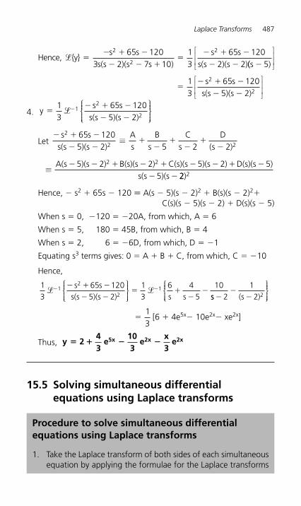
Laplace Transforms 487
Hence, �{y}s s
s(s )(s s )s s
s(s )(s )�
� � �
� � ��
� � �
� �
2
2
265 1203 2 7 10
13
65 1202 2 ((s )� 5
⎡
⎣⎢⎢
⎤
⎦⎥⎥
�� � �
� �
13
65 1205 2
2
2
s ss(s )(s )
⎡
⎣⎢⎢
⎤
⎦⎥⎥
4. ys s
s(s )(s )�
� � �
� ��1
365 1205 2
12
2�
⎧⎨⎪⎪⎩⎪⎪
⎫⎬⎪⎪⎭⎪⎪
Let � � �
� ��
��
��
�
s ss(s )(s )
As
Bs
Cs
D(s )
2
2 2
65 1205 2 5 2 2
≡
≡A(s )(s ) B(s)(s ) C(s)(s )(s ) D(s)(s )
s(s )(s� � � � � � � � �
� �
5 2 2 5 2 55
2 2
22 2)
Hence, � s 2 � 65s � 120 � A(s � 5)(s � 2) 2 � B(s)(s � 2) 2 � C(s)(s � 5)(s � 2) � D(s)(s � 5)
When s � 0, � 120 � � 20A, from which, A � 6
When s � 5, 180 � 45B, from which, B � 4
When s � 2, 6 � � 6D, from which, D � � 1
Equating s 3 terms gives: 0 � A � B � C, from which, C � � 10
Hence,
13
65 1205 2
13
6 45
1012
21� �� �� � �
� �� �
��
s ss(s )(s ) s s
⎧⎨⎪⎪⎩⎪⎪
⎫⎬⎪⎪⎭⎪⎪ ss (s )�
��212 2
⎧⎨⎪⎪⎩⎪⎪
⎫⎬⎪⎪⎭⎪⎪
�13
[6 � 4e 5x � 10e 2x � xe 2x ]
Thus, y 243
e103
ex3
e5x 2x 2x� � � �
15.5 Solving simultaneous differential equations using Laplace transforms
Procedure to solve simultaneous differential equations using Laplace transforms
1. Take the Laplace transform of both sides of each simultaneous equation by applying the formulae for the Laplace transforms
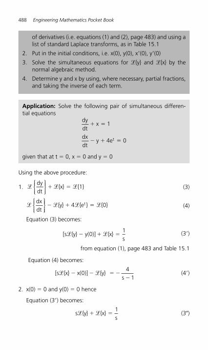
488 Engineering Mathematics Pocket Book
of derivatives (i.e. equations (1) and (2), page 483) and using a list of standard Laplace transforms, as in Table 15.1
2. Put in the initial conditions, i.e. x(0), y(0), x � (0), y�(0)
3. Solve the simultaneous equations for � { y } and � { x } by the normal algebraic method.
4. Determine y and x by using, where necessary, partial fractions, and taking the inverse of each term.
Application: Solve the following pair of simultaneous differen-tial equations
dydt
x
dxdt
y et
� �
� � �
1
4 0
given that at t � 0, x � 0 and y � 0
Using the above procedure:
1. � � �dydt
{x} {1}⎧⎨⎪⎪⎩⎪⎪
⎫⎬⎪⎪⎭⎪⎪
� � (3)
� � � �dxdt
{y} {e } { }t⎧⎨⎪⎪⎩⎪⎪
⎫⎬⎪⎪⎭⎪⎪
� � �4 0 (4)
Equation (3) becomes:
[s {y} y( )] {x}s
� �� � �01 (3 � )
from equation (1), page 483 and Table 15.1
Equation (4) becomes:
[s {x} x( )] {y} s
� �� � � ��
04
1(4� )
2. x(0) � 0 and y(0) � 0 hence
Equation (3 � ) becomes:
s {y} {x}s
� �� �1
(3 � )
Laplace Transforms 489
and equation (4 � ) becomes: s � { x } � � { y } � ��
41s
or � � � ��
� �{y} s {x}s
41
(4� )
3. 1 � equation (3 � ) and s � equation (4� ) gives:
s {y} {x}
s� �� �
1 (5)
� � � �
�s {y} s {x}
ss
� �2 41
(6)
Adding equations (5) and (6) gives:
(s ) {x}s
ss
(s ) s( s)s(s )
s ss(s )
2 � � ��
�� �
��
� � �
�1
1 41
1 41
4 11
2�
from which, �{x}s s
s(s )(s )�
� � �
� �
4 11 1
2
2
Using partial fractions
� � �
� ��
��
�
�
�� � �
4 11 1 1
1 1
2
2 2
2
s ss(s )(s )
As
B(s )
Cs D(s 1)
A(s )(s ) B s (
≡
ss ) (Cs D) s (s )s(s )(s )
2
2
1 11 1
� � �
� �
+
Hence, � 4s2 � s � 1 � A(s � 1)(s2 � 1) � Bs(s2 � 1) � (Cs � D)s(s � 1)
When s � 0, � 1 � �A hence, A � 1
When s � 1, � 4 � 2B hence, B � � 2
Equating s 3 coefficients:
0 1 2� � � � � �A B C hence, (since A and B )C 1�
Equating s 2 coefficients:
� � � � � � �4 1 1A D C hence (since A and C )D 2� �
Thus, �{x}s s
s(s s (ss
(s�
� � �
� �� �
��
�
�
4 11 1
1 21
21
2
2 2)( ) ) )s
490 Engineering Mathematics Pocket Book
4.
Hence, xs (s
s(s
s (s
� ��
��
�
� �
�
�
�
�
12
1
1 21
21
1 2
) )
⎧⎨⎪⎪⎩⎪⎪
⎫⎬⎪⎪⎭⎪⎪
���
��
�1 12
12 2)s
(s ) (s )
⎧⎨⎪⎪⎩⎪⎪
⎫⎬⎪⎪⎭⎪⎪
i.e. x � 1 � 2e t � cos t � 2 sin t from Table 15.1 , page 472
The second equation given originally is dxdt
y et� � �4 0
from which, ydxdt
eddt
t� � �4 (1 � 2et � cos t � 2 sin t) � 4et
� � � � �2 2 4e sin t cos t et t
i.e. y � 2e t � sin t �2 cos t
[Alternatively, to determine y, return to equations (3 � � ) and (4��)]
Application: Solve the following pair of simultaneous differen-tial equations
d xdt
x y
d ydt
y x
2
2
2
2
� �
� � �
given that at t � 0, x � 2, y ��1,dxdt
� 0 and dydt
� 0
1. [s {x} s x( ) x ( )] {x} {y}2 0 0� � �� � � �′ (7)
[s {y} s y( ) y ( )] {y} {x}2 0 0� � �� � � � �′ (8)
2. x(0) � 2, y(0) � � 1, x � (0) � 0 and y � (0) � 0
hence s {x} 2s {x} {y}2� � �� � � (7� )
s {y} s {y} {x}2� � �� � � � (8� ) 3. Rearranging gives:
(s ) {x} {y} s2 1 2� � �� � (9)
� �{x} (s ) {y} s� � � �2 1 (10)
Laplace Transforms 491
Equation (9) � (s 2 � 1) and equation (10) � 1 gives:
(s )(s ) {x} (s ) {y} (s ) s2 2 2 21 1 1 12� � � � � �� � (11)
� �{x} (s ) {y} s� � � �2 1 (12)
Adding equations (11) and (12) gives:
[(s )(s ) ] {x} (s ) s s2 2 21 1 1 12� � � � � ��
i.e. s 4 � { x} � 2s 3 � s � s(2s 2 � 1)
from which, �{x}s ( s )
sss
ss s s s
��
��
� � � �2 1 2 1 2 1 2 12
4
2
3
2
3 3 3
4. Hence xs s
� ��� 13
2 1⎧⎨⎪⎪⎩⎪⎪
⎫⎬⎪⎪⎭⎪⎪
i.e. x 212
t2� �
Returning to equations (9) and (10) to determine y:
1 � equation (9) and (s 2 � 1) � equation (10) gives:
(s ) {x} {y} s2 1 2� � �� � (13) (s ) {x} (s )(s ) {y} s(s )2 2 2 21 1 1 1� � � � � � �� � (14)
Equation (13) � equation (14) gives:
[ (s )(s )] {y} s s(s )� � � � � � �1 1 1 2 12 2 2�
i.e. � s 4 � { y } � s 3 � s
and �{ y}s s
s s s�
�
�� � �
3
4 3
1 1
from which, ys s
� � ��� 13
1 1⎧⎨⎪⎪⎩⎪⎪
⎫⎬⎪⎪⎭⎪⎪
i.e. y 112
t2� � �
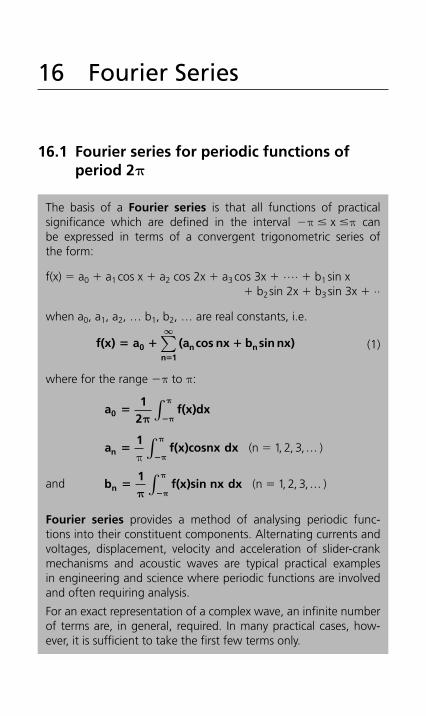
16 Fourier Series
16.1 Fourier series for periodic functions of period 2 π
The basis of a Fourier series is that all functions of practical significance which are defined in the interval � π � x � π can be expressed in terms of a convergent trigonometric series of the form:
f(x) � a 0 � a 1 cos x � a 2 cos 2x � a 3 cos 3x � … . � b 1 sin x � b 2 sin 2x � b 3 sin 3x � ..
when a 0 , a 1 , a 2 , … b 1 , b 2 , … are real constants, i.e.
f(x) a0� � ��
(a cos nx b sin nx)n nn 1
∞
∑ (1)
where for the range � π to π :
a1
2f(x)dx0 �
�π π
π
∫
a
1f(x)cosnx dxn �
�π )( , , ,n � 1 2 3 …∫ π
π
and b1
f(x)sin nx dxn ��π π
π ( )n � 1 2 3, , ,…∫
Fourier series provides a method of analysing periodic func-tions into their constituent components. Alternating currents and voltages, displacement, velocity and acceleration of slider-crank mechanisms and acoustic waves are typical practical examples in engineering and science where periodic functions are involved and often requiring analysis.
For an exact representation of a complex wave, an infinite number of terms are, in general, required. In many practical cases, how-ever, it is sufficient to take the first few terms only.
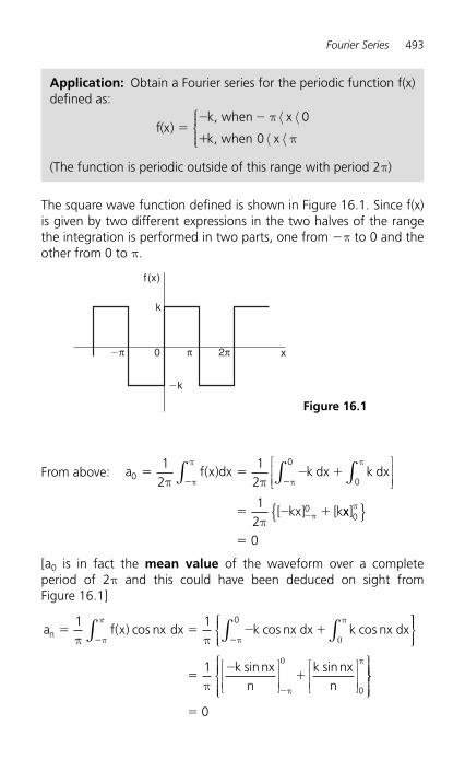
Fourier Series 493
The square wave function defined is shown in Figure 16.1 . Since f(x) is given by two different expressions in the two halves of the range the integration is performed in two parts, one from � π to 0 and the other from 0 to π .
Application: Obtain a Fourier series for the periodic function f(x) defined as:
f x
k
k x( )
, when x
, when �
� �
�
π
π
⟨ ⟨
⟨ ⟨
⎧⎨⎪⎪
⎩⎪⎪
0
0
(The function is periodic outside of this range with period 2 π )
Figure 16.1
0
k
�k
�π π 2π
f (x)
x
From above: a f x k k dx
kx k
0
0
0
12
12
12
� � � �
� � �
� �
�
π π
π
π
π π
π
π
( )
[ ] [
dx dx0∫ ∫∫
⎡
⎣⎢⎢
⎤
⎦⎥⎥
xx]0
0
π{ }
� [a 0 is in fact the mean value of the waveform over a complete period of 2 π and this could have been deduced on sight from Figure 16.1 ]
a f x nx k kn � � � �� �
1 1 0
π π 0
π
π( ) cos cos cos dx nx dx nx dx
π
π
∫ ∫∫⎧⎨⎪⎪⎩⎪⎪
⎫⎫⎬⎪⎪⎭⎪⎪
⎡
⎣⎢⎢
⎤
⎦⎥⎥
⎡
⎣⎢⎢
⎤
⎦⎥⎥
⎧⎨⎪⎪⎪
⎩⎪⎪⎪
⎫�
��
�
1
0π π
0 πk
nk
nsin sinnx nx
⎬⎬⎪⎪⎪
⎭⎪⎪⎪
� 0
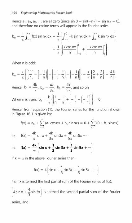
494 Engineering Mathematics Pocket Book
Hence a 1, a 2, a 3, … are all zero (since sin 0 � sin(�nπ) � sin n π � 0),and therefore no cosine terms will appear in the Fourier series.
b f x k kn � � � �� �
1 1 0
π ππ
π
0
π
π( ) sin sin sinnx dx nx dx nx dx∫ ∫∫
⎧⎨⎪⎪⎩⎪⎪
⎫⎫⎬⎪⎪⎭⎪⎪
⎡
⎣⎢⎢
⎤
⎦⎥⎥
⎡
⎣⎢⎢
⎤
⎦⎥⎥
⎧⎨⎪⎪⎪
⎩⎪⎪⎪
⎫� �
�
�
10
0π π
πk
nk
ncos cosnx nx
⎬⎬⎪⎪⎪
⎭⎪⎪⎪
When n is odd:
bk
n n nn � � � � � � �π
1 1 1⎛⎝⎜⎜⎜
⎞⎠⎟⎟⎟⎟
⎛⎝⎜⎜⎜
⎞⎠⎟⎟⎟⎟
⎡
⎣⎢⎢
⎤
⎦⎥⎥
⎛⎝⎜⎜⎜
⎞⎠⎟⎟⎟⎟ �� � �
1 2 2n
kn n
⎛⎝⎜⎜⎜
⎞⎠⎟⎟⎟⎟
⎡
⎣⎢⎢
⎤
⎦⎥⎥
⎧⎨⎪⎪
⎩⎪⎪
⎫⎬⎪⎪
⎭⎪⎪
⎧⎨⎪⎪⎩⎪⎪
⎫⎬⎪⎪⎭⎪π ⎪⎪
�4 knπ
Hence, b1k
�4π
, b343
�kπ
, b545
�kπ
, and so on
When n is even: bk
n n n nn � � � � � �π
1 1 1 1⎡
⎣⎢⎢
⎤
⎦⎥⎥
⎛⎝⎜⎜⎜
⎞⎠⎟⎟⎟⎟
⎡
⎣⎢⎢
⎤
⎦⎥⎥
⎧⎨⎪⎪
⎩⎪⎪
⎫⎬⎪⎪
⎭⎪⎪⎪� 0
Hence, from equation (1), the Fourier series for the function shown in Figure 16.1 is given by:
f x a a nx b bn n
nn
n
( ) ( cos sin ) ( sin )� � � � � �� �
�
01 1
0 0nx nx�
∑ ∑
i.e. f x x xk
x( ) sin sin sin ..� � � �4 4
33
45
5k k
π π π
i.e. f(x)4k
sin x13
sin 3x15
sin 5x ...� � � �π
⎛⎝⎜⎜⎜
⎞⎠⎟⎟⎟⎟
If k � π in the above Fourier series then:
f x x x( ) sin sin sin� � �413
315
5+ …⎛⎝⎜⎜⎜
⎞⎠⎟⎟⎟⎟x
4 sin x is termed the first partial sum of the Fourier series of f(x),
443
3sin sinx x�⎛⎝⎜⎜⎜
⎞⎠⎟⎟⎟⎟ is termed the second partial sum of the Fourier
series, and
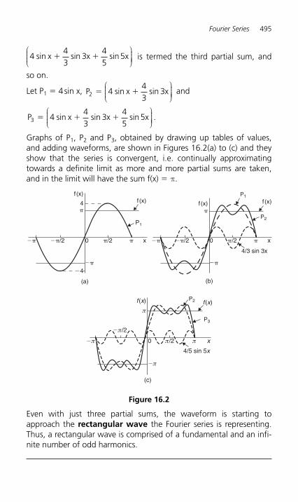
Fourier Series 495
443
345
5sin sin sinx x x� �⎛⎝⎜⎜⎜
⎞⎠⎟⎟⎟⎟ is termed the third partial sum, and
so on.
Let P 1 � 4 sin x, P x x2 443
3� �sin sin⎛⎝⎜⎜⎜
⎞⎠⎟⎟⎟⎟ and
P x x x3 443
345
5� � �sin sin sin .⎛⎝⎜⎜⎜
⎞⎠⎟⎟⎟⎟
Graphs of P 1, P 2 and P 3, obtained by drawing up tables of values, and adding waveforms, are shown in Figures 16.2(a) to (c) and they show that the series is convergent, i.e. continually approximating towards a definite limit as more and more partial sums are taken, and in the limit will have the sum f(x) � π .
4�
��
��
��/2 �/2
P1
f(x)f (x)
x�0
�4
(a)
�
��
��
��/2 �/2
P2
f(x)f (x)
x�0
P1
(b)
4/3 sin 3x
π
�π
�π
π/2
�π/2
P3
f (x)f (x)
xπ0
P2
(c)
4/5 sin 5x
Figure 16.2
Even with just three partial sums, the waveform is starting to approach the rectangular wave the Fourier series is representing. Thus, a rectangular wave is comprised of a fundamental and an infi-nite number of odd harmonics.
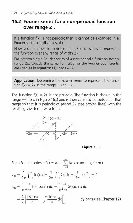
496 Engineering Mathematics Pocket Book
16.2 Fourier series for a non-periodic function over range 2 π
If a function f(x) is not periodic then it cannot be expanded in a Fourier series for all values of x.
However, it is possible to determine a Fourier series to represent the function over any range of width 2 π .
For determining a Fourier series of a non-periodic function over a range 2 π, exactly the same formulae for the Fourier coefficients are used as in equation (1), page 492.
Application: Determine the Fourier series to represent the func-tion f(x) � 2x in the range � π to � π
The function f(x) � 2x is not periodic. The function is shown in the range � π to π in Figure 16.3 and is then constructed outside of that range so that it is periodic of period 2 π (see broken lines) with the resulting saw-tooth waveform.
���2�
�2�
2�
2�
3��
f (x) f (x) � 2x
x0
Figure 16.3
For a Fourier series: f x a a bn nn
( ) ( cos sin )� � ��
01
nx nx∞
∑
a f x dx x x
a f xn
021
21
22
12
0
1
� � � �
�
� ��π π π
π
π
π
π
π
π
π( )
( ) cos
dx∫∫ ⎡⎣⎢
⎤⎦⎥
nnx dx nx dx
nx nxdx b
�
� �
�� �
�
1
2
π2
π
π
π
π
π
π
∫ ∫
∫⎡
⎣⎢⎢
⎤
⎦⎥⎥
x
xn n
cos
sin sinyy parts (see Chapter 12)
Fourier Series 497
� � � �
�
�
2 20
0
2 2π ππ
π
πx
nnx
nn
nsin cos cosnx⎡
⎣⎢⎢
⎤
⎦⎥⎥
⎛⎝⎜⎜⎜
⎞⎠⎟⎟⎟⎟
⎡
⎣⎢⎢
���
�
� �
cos ( )
( ) sin sin
nn
b f x xn
π
π π
20
1 12
⎛⎝⎜⎜⎜
⎞⎠⎟⎟⎟⎟⎤
⎦⎥⎥
nx dx nx dxx
nx nxn
dx by p
��
�
��
��
π
π
π
π
π
π
π
∫∫
∫⎛⎝⎜⎜⎜
⎞⎠⎟⎟⎟⎟
⎡
⎣⎢⎢
⎤
⎦⎥⎥
2 x coxn
cosaarts
x nx nx
n
��
�
��
�
�
2
2
2
2
π
ππ π π
π
πcos sin
cos sin
n n
n nn
⎡
⎣⎢⎢
⎤
⎦⎥⎥
⎛⎝⎜⎜⎜⎜
⎞⎠⎟⎟⎟⎟
⎛⎝⎜⎜⎜
⎞⎠⎟⎟⎟⎟
⎡
⎣⎢⎢
⎤
⎦⎥⎥�
� � ��
�
��
( ) cos ( ) sin ( )π π π
ππ
nn
nn2
2 ccos cos( )cos
cos cos
nn
nn n
n
n
π π ππ
π π
��
��
� �
⎡
⎣⎢⎢
⎤
⎦⎥⎥
4
since n ( )
When n is odd, bnn �4
. Thus b 1 � 4, b343
� , b545
� , and so on.
When n is even, bnn � �4 . Thus b2
42
� � , b444
� � , b646
� � ,
and so on.
Thus , f x x x x x x( ) sin sin sin sin� � � � �2 442
243
344
4
� � �45
546
6sin sin ..x x
i.e. 2x 4(sin x12
sin 2x13
sin 3x14
sin 4x� � � �
� � �15
sin 5x16
sin 6x ...)
for values of f(x) between � π and π .
498 Engineering Mathematics Pocket Book
16.3 Even and odd functions
A function y � f(x) is said to be even if f( � x) � f(x) for all values of x. Graphs of even functions are always symmetrical about the y-axis (i.e. a mirror image). Two examples of even functions are y � x 2 and y � cos x as shown in Figure 6.38, page 181.
A function y � f(x) is said to be odd if f( � x) � � f(x) for all values of x. Graphs of odd functions are always symmetrical about the origin. Two examples of odd functions are y � x 3 and y � sin x as shown in Figure 6.39, page 181.
Many functions are neither even nor odd, two such examples being y � ln x and y � e x .
Fourier cosine series
The Fourier series of an even periodic function f(x) having period 2π contains cosine terms only (i.e. contains no sine terms) and may contain a constant term.
Hence f(x) a a cos nx0 nn 1
� ��
�
∑ (2)
where a1
f(x) dx00
�1
2π π
πf x dx( ) �
�∫ ∫π
π (due to symmetry)
and a2
f(x) cos nx dxn � ��
1π
f x( ) cos nx dxπ
π
∫ ∫π
π
0
Fourier sine series
The Fourier series of an odd periodic function f(x) having period 2π contains sine terms only (i.e. contains no constant term and no cosine terms).
Hence f(x) b sin nxnn 1
��
�
∑ (3)
where b2
f(x) sin nx dxn0
� ��
1π π
πf x( ) sin nx dx∫ ∫π
π
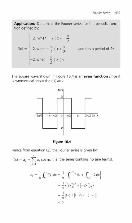
Fourier Series 499
Hence from equation (2), the Fourier series is given by:
f x a ann
( ) cos� ��
�
01
nx∑ (i.e. the series contains no sine terms).
a f x dx
x
00
2
2
0
1 12 2
12
� � � �
�
π π
π
0
π π
π
π
π
( )∫ ∫ ∫⎧⎨⎪⎪⎩⎪⎪
⎫⎬⎪⎪⎭⎪⎪
[ ]
dx dx/
/
///
22
2
12
0
� �
� � � � �
�
x[ ]{ }[ ]⎡
⎣⎢⎤⎦⎥
ππ
ππ π π)( ) ( ) (
Application: Determine the Fourier series for the periodic func-tion defined by:
f x( )
,
,
,
�
� � �
�
�
22
22 2
22
when x
when x
when x
ππ
π π
ππ
⟨ ⟨
⟨ ⟨
⟨ ⟨
⎧
⎨
⎪⎪⎪⎪⎪⎪⎪⎪⎪⎪
⎩
⎪⎪⎪⎪⎪⎪⎪⎪⎪
and has a period of 2π
0�π/2 π/2�3π/2
�2
2
3π/2 2π�π π
f (x)
x
Figure 16.4
The square wave shown in Figure 16.4 is an even function since it is symmetrical about the f(x) axis.
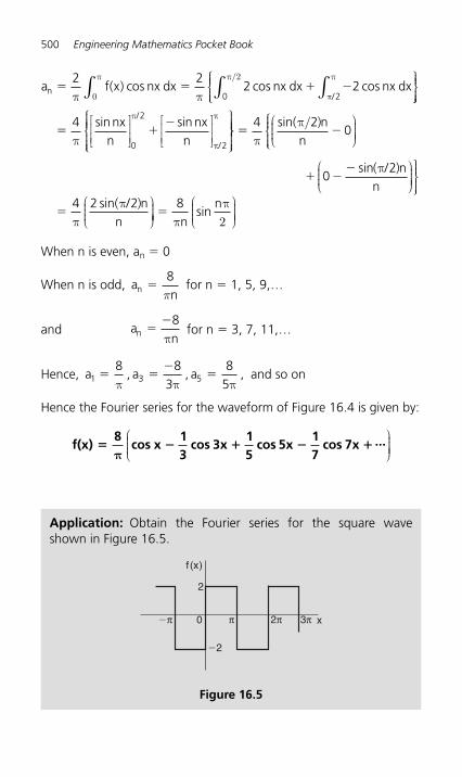
500 Engineering Mathematics Pocket Book
a f x nx nxn � � � �2 2
2 220π π π
ππ/2( ) cos cos cosdx dx nx dx
/∫∫⎧⎨⎪⎪⎩⎪⎪
⎫⎬⎪⎪⎭⎭⎪⎪
⎡
⎣⎢⎢
⎤
⎦⎥⎥
⎡
⎣⎢⎢
⎤
⎦⎥⎥
⎧⎨⎪⎪⎪
⎩⎪⎪⎪
⎫
∫0
π
π
π
π
π� �
�4
0
2
2
sin sinnx nxn
/
/n⎬⎬⎪⎪⎪
⎭⎪⎪⎪
⎛⎝⎜⎜⎜
⎞⎠⎟⎟⎟⎟
⎧⎨⎪⎪⎩⎪⎪
� �4 2
0π
π/sin( )nn
/
/
� ��
�
02
4 2 2
sin( )
sin( )
π
ππ
nn
nn
⎛⎝⎜⎜⎜
⎞⎠⎟⎟⎟⎟⎫⎬⎪⎪⎭⎪⎪
⎛⎝⎜⎜⎜
⎞⎠⎟⎟⎟⎟⎟
⎛⎝⎜⎜⎜
⎞⎠⎟⎟⎟⎟�
8π
π2n
nsin
When n is even, a n � 0
When n is odd, ann �
8π
for n � 1, 5, 9, …
and an ��8πn
for n � 3, 7, 11, …
Hence, a a a1 3 58 8
38
5� �
��
π π π, , , and so on
Hence the Fourier series for the waveform of Figure 16.4 is given by:
f(x)
8cos x
13
cos 3x15
cos 5x17
cos 7x ...� � � � �π
⎛⎝⎜⎜⎜
⎞⎠⎟⎟⎟⎟
Application: Obtain the Fourier series for the square wave shown in Figure 16.5 .
0
2
�2
�π π 2π 3π
f (x)
x
Figure 16.5
Fourier Series 501
The square wave is an odd function since it is symmetrical about the origin.
Hence, from equation (3), the Fourier series is given by:
f x bnn
( ) sin��
nx1
�
∑
The function is defined by: f xx
x( )
,
,�
� �2 0
2 0
when
when
π
π
⟨ ⟨
⟨ ⟨
⎧⎨⎪⎪
⎩⎪⎪
b f xnn � � �
�
��
2 22
4
4
0 0π π π
π
π
0
π( ) sin sin
cos
c
nx dx nx dxnx
∫ ∫⎡
⎣⎢⎢
⎤
⎦⎥⎥
π
oos( cos )
nn n n
nπ
ππ
⎛⎝⎜⎜⎜
⎞⎠⎟⎟⎟⎟
⎛⎝⎜⎜⎜
⎞⎠⎟⎟⎟⎟
⎡
⎣⎢⎢
⎤
⎦⎥⎥� � � �
1 41
When n is even, b n � 0. When n is odd, bn nn � � � �
41 1
8π π
[ ( )]
Hence, b b b1 3 58 8
38
5� � �
π π π, , , and so on
Hence the Fourier series is:
f(x)
8sin x
13
sin 3x15
sin 5x17
sin 7x ...� � � � �π
( )
16.4 Half range Fourier series
When a function is defined over the range say 0 to π instead of from 0 to 2 π it may be expanded in a series of sine terms only or of cosine terms only. The series produced is called a half-rangeFourier series .
When a half range cosine series is required then:
f(x) a a cos nx0 nn 1
� ��
�
∑ (4)
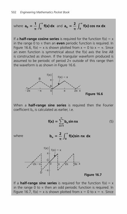
502 Engineering Mathematics Pocket Book
where a1
f(x) dx00
�π
π
∫ and a2
f(x) cos nx dxn0
�π
π
∫
If a half-range cosine series is required for the function f(x) � x in the range 0 to π then an even periodic function is required. In Figure 16.6 , f(x) � x is shown plotted from x � 0 to x � π. Since an even function is symmetrical about the f(x) axis the line AB is constructed as shown. If the triangular waveform produced is assumed to be periodic of period 2 π outside of this range then the waveform is as shown in Figure 16.6.
When a half-range sine series is required then the Fourier coefficient b n is calculated as earlier, i.e.
f(x) b sin nxnn 1
��
�
∑ (5)
where b2
f(x)sin nx dxn0
�π
π
∫
If a half-range sine series is required for the function f(x) � x in the range 0 to π then an odd periodic function is required. In Figure 16.7 , f(x) � x is shown plotted from x � 0 to x � π. Since
�2π 2π0
A
B
�π π
π
f (x)f (x) � x
x Figure 16.6
2π 3π0C
D
�π�2π π
π
�π
f (x)f (x) � x
x
Figure 16.7
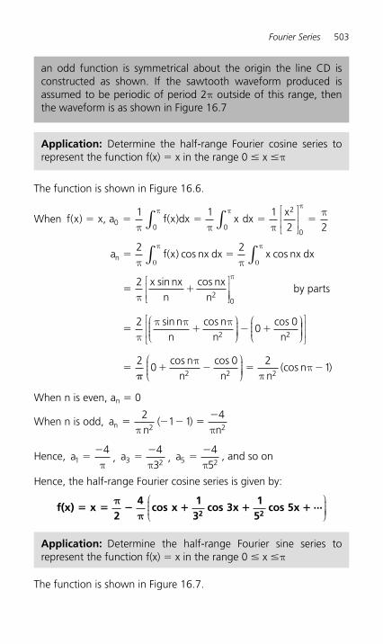
Fourier Series 503
The function is shown in Figure 16.6.
When f x x a f x dx xx
( ) ( )� � � � �, dx00 0
2
0
1 1 12 2π π π
ππ ππ
∫ ∫⎡
⎣⎢⎢
⎤
⎦⎥⎥
a f x nx x
xn n
n � �
� �
2 2
22
π π
π
0
π
0
π( ) cos cos
sin cos
dx nx dx
nx nx
∫ ∫⎡
⎣⎢⎢
⎤
⎦⎥⎥⎥
⎛⎝⎜⎜⎜
⎞⎠⎟⎟⎟⎟
⎛⎝⎜⎜⎜
⎞⎠
0
2 2
20
0
π
ππ π π
by parts
� � � �sin cos cosn
nn
n n⎟⎟⎟⎟⎟
⎡
⎣⎢⎢
⎤
⎦⎥⎥
⎛⎝⎜⎜⎜
⎞⎠⎟⎟⎟⎟�
�� � � �
20
0 21
2 2 2
cos cos(cos )
nn n n
nπ
ππ
When n is even, a n � 0
When n is odd, an nn � � � �
�21 1
42 2π π
( )
Hence, a14
��
π , a3 2
43
��
π , a5 2
45
��
π , and so on
Hence, the half-range Fourier cosine series is given by:
f(x) x
24
cos x13
cos 3x1
5cos 5x ...
2 2� � � � � �
ππ
⎛⎝⎜⎜⎜
⎞⎠⎟⎟⎟⎟
an odd function is symmetrical about the origin the line CD is constructed as shown. If the sawtooth waveform produced is assumed to be periodic of period 2 π outside of this range, then the waveform is as shown in Figure 16.7
Application: Determine the half-range Fourier cosine series to represent the function f(x) � x in the range 0 � x � π
Application: Determine the half-range Fourier sine series to represent the function f(x) � x in the range 0 � x � π
The function is shown in Figure 16.7 .
504 Engineering Mathematics Pocket Book
When f(x) � x,
b f x nx dx xn � �2 2
0 0π π
π π( ) sin sin∫ ∫ nx dx
��
�
��
�
2
2
20
2
π
ππ π π
πx
n n
nn
nn
cos sin
cos sin
nx nxby parts
⎡
⎣⎢⎢
⎤
⎦⎥⎥
⎛⎝⎜⎜⎜⎜
⎞⎠⎟⎟⎟⎟
⎡
⎣⎢⎢
⎤
⎦⎥⎥� � � �( ) cos0 0
2n
nπ
When n is odd, bnn �2
. Hence, b121
� , b323
� , b525
� and so on.
When n is even, bnn � �2
. Hence b222
� � , b424
� � , b626
� �
and so on
Hence the half-range Fourier sine series is given by:
f(x) x
2 sin x12
sin 2x13
sin 3x14
sin 4x15
sin 5x ...
�
� � � � � �⎛⎝⎜⎜⎜
⎞⎠⎟⎟⎟⎟⎟
16.5 Expansion of a periodic function of period L
If f(x) is a function of period L, then its Fourier series is given by:
f(x) a a cos2 nx
Lb sin
nxL0 n n� � �
π 2π⎛⎝⎜⎜⎜
⎞⎠⎟⎟⎟⎟
⎛⎝⎜⎜⎜
⎞⎠⎟⎟⎟⎟
⎡
⎣⎢⎢
⎤
⎦⎥⎥⎥∑
n 1�
�
(6)
where, in the range �L2
to �L2
:
a
1L
f(x)dx, a2L
f(x)cos2 nx
Ldx0 n
L/2
L/2
L/2
L/2� �
��
π⎛⎝⎜⎜⎜
⎞⎠⎟⎟⎟⎟∫∫
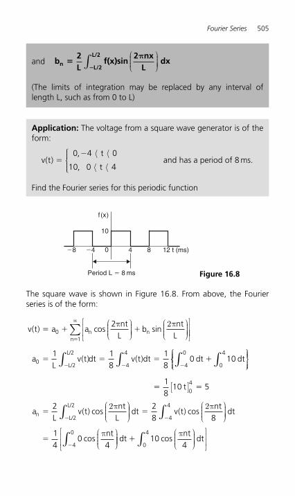
Fourier Series 505
and b2L
f(x)sin2 nx
Ldxn
L/2
L/2�
�
π⎛⎝⎜⎜⎜
⎞⎠⎟⎟⎟⎟∫
(The limits of integration may be replaced by any interval of length L, such as from 0 to L)
Application: The voltage from a square wave generator is of the form:
v t
t
t( )
,
,�
�0 4 0
10 0 4
⟨ ⟨
⟨ ⟨
⎧⎨⎪⎪
⎩⎪⎪and has a period of 8 ms.
Find the Fourier series for this periodic function
0
10
�4 4 8 12 t (ms)
Period L � 8 ms
�8
f(x)
Figure 16.8
The square wave is shown in Figure 16.8 . From above, the Fourier series is of the form:
v t a ant
Lb
ntLn n( ) cos sin� � �0
2π 2π⎛⎝⎜⎜⎜
⎞⎠⎟⎟⎟⎟
⎛⎝⎜⎜⎜
⎞⎠⎟⎟⎟⎟
⎡
⎣⎢⎢
⎤
⎦⎥⎥⎥
⎧
∑
∫ ∫ ∫ ∫
n
L
La
Lv t v t
�
� � �� � � �
1
04
4
4
0
0
41 18
18
0 10
�
( ) ( )/2
/2dt dt dt dt⎨⎨
⎪⎪⎩⎪⎪
⎫⎬⎪⎪⎭⎪⎪
[ ]
⎛⎝⎜⎜⎜
⎞⎠∫
� �
��
18
10 5
2
04t
aL
v tnt
LnL
L( ) cos
/2
/2 2π ⎟⎟⎟⎟⎟⎛⎝⎜⎜⎜
⎞⎠⎟⎟⎟⎟
⎛⎝⎜⎜⎜
⎞⎠⎟
∫dt dt�
�
�
28 8
14
04
4
4v t
nt
nt
( ) cos
cos
2π
π⎟⎟⎟⎟
⎛⎝⎜⎜⎜
⎞⎠⎟⎟⎟⎟
⎡
⎣⎢⎢
⎤
⎦⎥⎥∫∫ dt
ntdt�
�10
40
4
4
0cos
π
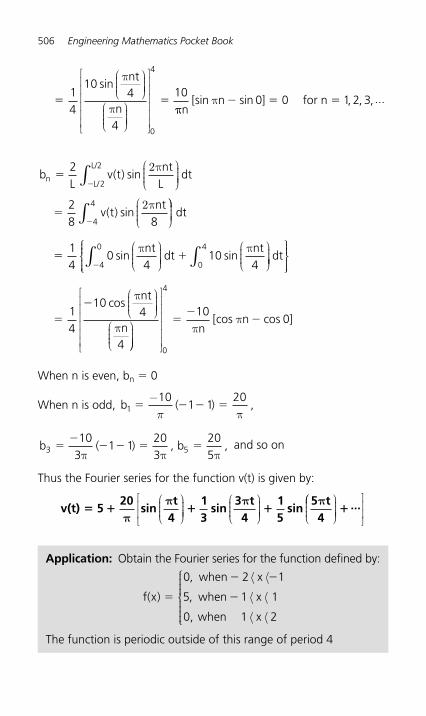
506 Engineering Mathematics Pocket Book
bL
v tL
v t
nL
L�
�
�
2
28 8
2( ) sin
( ) sin
2π
2π
ntdt
nt
/
/2 ⎛⎝⎜⎜⎜
⎞⎠⎟⎟⎟⎟
⎛⎝⎜⎜⎜
∫⎞⎞⎠⎟⎟⎟⎟
⎛⎝⎜⎜⎜
⎞⎠⎟⎟⎟⎟
⎛⎝⎜⎜⎜
⎞⎠⎟⎟⎟
∫�
� �
4
4
14
0 10
dt
nt4
dtnt4
sin sinπ π
⎟⎟⎧⎨⎪⎪⎩⎪⎪
⎫⎬⎪⎪⎭⎪⎪
⎛⎝⎜⎜⎜
⎞⎠⎟⎟⎟⎟
⎛⎝⎜⎜⎜
⎞
∫∫ dt
nt4
0
4
4
0
14
10
4
�
�
� cosπ
πn⎠⎠⎟⎟⎟⎟
⎡
⎣
⎢⎢⎢⎢⎢⎢
⎤
⎦
⎥⎥⎥⎥⎥⎥0
4
100�
��
ππ
nn[cos cos ]
When n is even, b n � 0
When n is odd, b110
1 120
� � � �−π
( )π
,
b b3 510
31 1
203
205
��
� � � �π π π
( ) , , and so on
Thus the Fourier series for the function v(t) is given by:
v(t) 5
20sin
t4
13
sin3 t4
15
sin5 t
4� � � �
ππ π π⎛
⎝⎜⎜⎜
⎞⎠⎟⎟⎟⎟
⎛⎝⎜⎜⎜
⎞⎠⎟⎟⎟⎟
⎛⎛⎝⎜⎜⎜
⎞⎠⎟⎟⎟⎟
⎡
⎣⎢⎢
⎤
⎦⎥⎥� ...
� �14
104
4
10
0
4
sinπ
π
nt⎛⎝⎜⎜⎜
⎞⎠⎟⎟⎟⎟
⎛⎝⎜⎜⎜
⎞⎠⎟⎟⎟⎟
⎡
⎣
⎢⎢⎢⎢⎢⎢
⎤
⎦
⎥⎥⎥⎥⎥⎥
n πππ
nn[sin sin ] , , ,� � �0 0 1 2 3 for n ...
Application: Obtain the Fourier series for the function defined by:
f x
x
x
x
( )
,
,�
� �
�
0 2 1
5 1
1 2
when
when 1
0, when
⟨ ⟨
⟨ ⟨
⟨ ⟨
⎧
⎨
⎪⎪⎪⎪
⎩⎪⎪⎪⎪
The function is periodic outside of this range of period 4
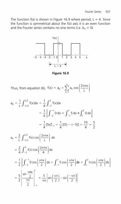
Fourier Series 507
The function f(x) is shown in Figure 16.9 where period, L � 4. Since the function is symmetrical about the f(x) axis it is an even function and the Fourier series contains no sine terms (i.e. b n � 0)
Thus, from equation (6), f x a aLn
n
( ) cos� ��
�
01
2πnx⎛⎝⎜⎜⎜
⎞⎠⎟⎟⎟⎟∑
aL
f x f x
dx
L
L
02
2
2
2
2
1
1
1
1 14
14
0 5
� �
� �
� �
�
�
�
( ) ( )dx dx
dx
/
/
∫ ∫
∫ ∫⎧⎨⎪⎪⎩⎪⎪
��
� � � � � ��
0
14
514
5 5104
52
1
2
11
dx∫⎫⎬⎪⎪⎭⎪⎪
[ ] [( ) ( )]x
aL
f xL
f x
nL
L�
�
2 2
24 4
2
2( ) cos
( ) cos
π
2π
nx dx
nx
/
/ ⎛
⎝⎜⎜⎜
⎞
⎠⎟⎟⎟⎟
=⎛
⎝⎜⎜
∫
⎜⎜⎞
⎠⎟⎟⎟⎟
⎛
⎝⎜⎜⎜
⎞
⎠⎟⎟⎟⎟
⎛
⎝⎜⎜⎜
⎞
⎠⎟⎟⎟⎟
∫�
� �
2
12
02
52
2
π π
dx
nxdx
nxcos cos ddx
nxdx
��
�
�
�
1
1
2
1
2
52
∫∫ ∫⎧⎨⎪⎪⎩⎪⎪
⎛
⎝⎜⎜⎜
⎞
⎠⎟⎟⎟⎟
⎫⎬⎪⎪⎭⎪⎪
0π
π
1
2cos
sinnnx2
2
52 2
1
1
π ππ π
n nn n
⎡
⎣
⎢⎢⎢⎢⎢
⎤
⎦
⎥⎥⎥⎥⎥
⎛
⎝⎜⎜⎜
⎞
⎠⎟⎟⎟⎟
⎛
⎝⎜⎜⎜
�
� ��
sin sin⎞⎞
⎠⎟⎟⎟⎟
⎡
⎣⎢⎢
⎤
⎦⎥⎥
0�2 �1 21 3 4 5 x
L � 4
�5 �4 �3
f(x)
5
Figure 16.9
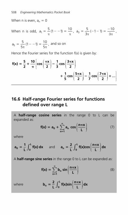
508 Engineering Mathematics Pocket Book
When n is even, a n � 0
When n is odd, a15
1 110
� � � �π π
( ) , a353
1 110
� � � ��
π 3π( ) ,
a55
51 1
105
� � � �π π
( ) , and so on
Hence the Fourier series for the function f(x) is given by:
f(x)52
10cos
x2
13
cos3 x
2� � �
ππ π⎛
⎝⎜⎜⎜
⎞⎠⎟⎟⎟⎟
⎛⎝⎜⎜⎜
⎞⎠⎟⎟⎟⎟
⎡
⎣⎢⎢
�15
cos5 x
2π⎛
⎝⎜⎜⎜
⎞⎠⎠⎟⎟⎟⎟
⎛⎝⎜⎜⎜
⎞⎠⎟⎟⎟⎟
⎤
⎦⎥⎥� �
17
cos7 x
2π
…
16.6 Half-range Fourier series for functions defined over range L
A half-range cosine series in the range 0 to L can be expanded as:
f(x) a a cosn x
L0 nn 1
� ��
� π⎛⎝⎜⎜⎜
⎞⎠⎟⎟⎟⎟∑ (7)
where
a
1L
f(x) dx a2L
f(x)cosn x
Ldx0
0
L
0
L� �∫ ∫
⎛⎝⎜⎜⎜
⎞⎠⎟⎟⎟⎟and n
π
A half-range sine series in the range 0 to L can be expanded as:
f(x) b sinn x
Lnn 1
��
�
∑⎛⎝⎜⎜⎜
⎞⎠⎟⎟⎟⎟
π(8)
where b
2L
f(x)sinn x
Ldxn
0
L�
π⎛⎝⎜⎜⎜
⎞⎠⎟⎟⎟⎟∫
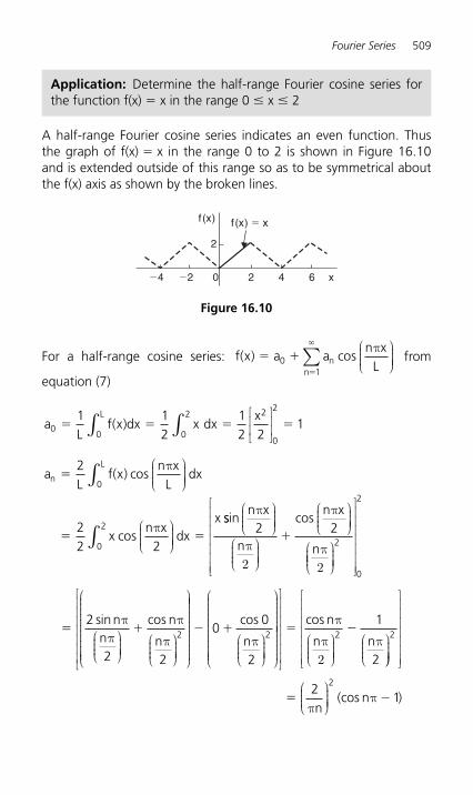
Fourier Series 509
A half-range Fourier cosine series indicates an even function. Thus the graph of f(x) � x in the range 0 to 2 is shown in Figure 16.10 and is extended outside of this range so as to be symmetrical about the f(x) axis as shown by the broken lines.
Application: Determine the half-range Fourier cosine series for the function f(x) � x in the range 0 � x � 2
0�2 2
2
4 6 x�4
f(x) f (x) � x
Figure 16.10
For a half-range cosine series: f x a an x
Lnn
( ) cos� ��
�
01
π⎛⎝⎜⎜⎜
⎞⎠⎟⎟⎟⎟∑ from
equation (7)
a
Lf x x
xL
00 0
2 2
0
21 1
212 2
1� � � �( )dx dx∫ ∫⎡
⎣⎢⎢
⎤
⎦⎥⎥
aL
f xn x
L
xn x
x
n
L�
� �
2
22
0( ) cos
cos
π
π
⎛⎝⎜⎜⎜
⎞⎠⎟⎟⎟⎟
⎛⎝⎜⎜⎜
⎞⎠⎟⎟⎟⎟
∫ dx
2dx
ssin cosn x
n
n x
n
π
π2
π
π2
2 2
⎛⎝⎜⎜⎜
⎞⎠⎟⎟⎟⎟
⎛⎝⎜⎜⎜
⎞⎠⎟⎟⎟⎟
⎛⎝⎜⎜⎜
⎞⎠⎟⎟⎟⎟
⎛⎝⎜
�
⎜⎜⎜⎞⎠⎟⎟⎟⎟
⎡
⎣
⎢⎢⎢⎢⎢⎢⎢
⎤
⎦
⎥⎥⎥⎥⎥⎥⎥
∫ 20
2
0
2
� �2
2 2
2
sin cosnn
n
n
ππ
π
π⎛⎝⎜⎜⎜
⎞⎠⎟⎟⎟⎟
⎛⎝⎜⎜⎜
⎞⎠⎟⎟⎟⎟
⎛
⎝
⎜⎜⎜⎜⎜⎜⎜⎜⎜⎜⎜⎜
⎞
⎠
⎟⎟⎟⎟⎟⎟⎟⎟⎟⎟⎟⎟⎟⎟⎛⎝⎜⎜⎜
⎞⎠⎟⎟⎟⎟
⎛
⎝
⎜⎜⎜⎜⎜⎜⎜⎜⎜⎜⎜⎜
⎞
⎠
⎟⎟⎟⎟⎟⎟� �00
2
2
cos
nπ⎟⎟⎟⎟⎟⎟⎟⎟
⎡
⎣
⎢⎢⎢⎢⎢⎢⎢
⎤
⎦
⎥⎥⎥⎥⎥⎥⎥
⎛⎝⎜⎜⎜
⎞⎠⎟⎟⎟⎟
⎛⎝⎜⎜⎜
⎞� �
cos n
n n
π
π2
π2
1
2 ⎠⎠⎟⎟⎟⎟
⎡
⎣
⎢⎢⎢⎢⎢⎢⎢
⎤
⎦
⎥⎥⎥⎥⎥⎥⎥
⎛⎝⎜⎜⎜
⎞⎠⎟⎟⎟⎟
2
22
1� �π
πn
n(cos )
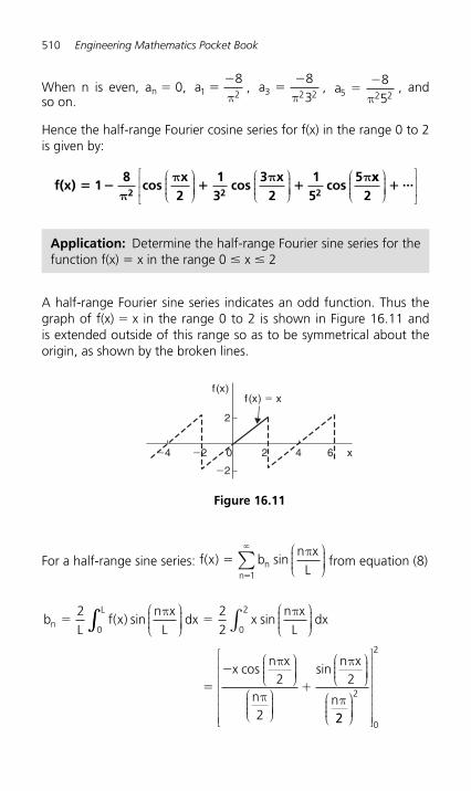
510 Engineering Mathematics Pocket Book
When n is even, a n � 0, a1 2
8�
�
π , a3 2 2
83
��
π , a5 2 2
85
��
π , and
so on.
Hence the half-range Fourier cosine series for f(x) in the range 0 to 2 is given by:
f(x) 1
8cos
x2
13
cos3 x
21
5cos
52 2 2
� � � �π
π π π⎛⎝⎜⎜⎜
⎞⎠⎟⎟⎟⎟
⎛⎝⎜⎜⎜
⎞⎠⎟⎟⎟⎟
xx2
...⎛⎝⎜⎜⎜
⎞⎠⎟⎟⎟⎟
⎡
⎣⎢⎢
⎤
⎦⎥⎥�
Application: Determine the half-range Fourier sine series for the function f(x) � x in the range 0 � x � 2
A half-range Fourier sine series indicates an odd function. Thus the graph of f(x) � x in the range 0 to 2 is shown in Figure 16.11 and is extended outside of this range so as to be symmetrical about the origin, as shown by the broken lines.
0�2 2
2
�2
4 6 x�4
f(x)f (x) � x
Figure 16.11
For a half-range sine series: f x bn x
Lnn
( ) sin��
π⎛⎝⎜⎜⎜
⎞⎠⎟⎟⎟⎟∑
1
�
from equation (8)
bL
f xn x
Ldx x
n xL
dxn
L� �
2 22 0
2
0( ) sin sin
π π⎛⎝⎜⎜⎜
⎞⎠⎟⎟⎟⎟
⎛⎝⎜⎜⎜
⎞⎠⎟⎟⎟⎟∫∫∫
⎛⎝⎜⎜⎜
⎞⎠⎟⎟⎟⎟
⎛⎝⎜⎜⎜
⎞⎠⎟⎟⎟⎟
⎛⎝⎜⎜⎜
⎞⎠⎟⎟⎟⎟
�
�
�
xn x
n
n x
n
cos sinπ
π
π
π
2
2
2
22
2
0
2
⎛⎝⎜⎜⎜
⎞⎠⎟⎟⎟⎟
⎡
⎣
⎢⎢⎢⎢⎢⎢⎢
⎤
⎦
⎥⎥⎥⎥⎥⎥⎥
Fourier Series 511
��
�2
2 2
2
cos sinnn
n
n
ππ
π
π⎛⎝⎜⎜⎜
⎞⎠⎟⎟⎟⎟
⎛⎝⎜⎜⎜
⎞⎠⎟⎟⎟⎟
⎛
⎝
⎜⎜⎜⎜⎜⎜⎜⎜
⎞
⎠
⎟⎟⎟⎟⎟⎟⎟⎟⎟⎛⎝⎜⎜⎜
⎞⎠⎟⎟⎟⎟
⎛
⎝
⎜⎜⎜⎜⎜⎜⎜⎜
⎞
⎠
⎟⎟⎟⎟⎟⎟⎟⎟
⎡
⎣
⎢⎢⎢⎢⎢
⎤
⎦
⎥� �00
2
2
sin
nπ ⎥⎥⎥⎥⎥
��
��2
2
4coscos
nn n
nπ
π ππ
Hence,b14
14
��
� �π π
( ) ,b24
21
42
��
��
π π( ) , b3
43
143
��
� �π π
( ) ,
and so on
Thus the half-range Fourier sine series in the range 0 to 2 is given by:
f(x) sinx
212
sin2 x
213
sin3 x
2� � �
4π
π π π⎛⎝⎜⎜⎜
⎞⎠⎟⎟⎟⎟
⎛⎝⎜⎜⎜
⎞⎠⎟⎟⎟⎟
⎛⎝⎜⎜⎜⎜
⎞⎠⎟⎟⎟⎟
⎡
⎣⎢⎢
�14
sin4 x
2π⎛
⎝⎜⎜⎜
⎞⎠⎟⎟⎟⎟ �� ...
⎤
⎦⎥⎥
16.7 The complex or exponential form of a Fourier series
The form used for the Fourier series considered previously con-sisted of cosine and sine terms. However, there is another form that is commonly used – one that directly gives the amplitude terms in the frequency spectrum and relates to phasor notation. This form involves the use of complex numbers (see Chapter 8). It is called the exponential or complex form of a Fourier series.
e j e jj jθ θθ θ θ θ� � � ��cos sin cos sinand
e ej jθ θ θ� �� 2 cos from which, cos
e e2
j jθ
θ θ�
� �
(9)
e e jj jθ θ θ� �� 2 sin from which, sin
e e2j
j jθ
θ θ�
� �
(10)
The complex or exponential form of the Fourier series.
f(x) c enn
j2 nx
L����
�
∑π
(11)
512 Engineering Mathematics Pocket Book
This is the same Application Problem as on page 506 and we can use this to demonstrate that the two forms of Fourier series are equivalent.
The function f(x) was shown in Figure 16.9 , where the period, L � 4.
From equation (11), the complex Fourier series is given by:
f x c enj
L
n
( ) ���
2πnx
�
�
∑
where c n is given by: cL
f x enj
LL
L
��
�
1 2
2
2 ( )πnx
dx∫ (from equation (12))
With reference to Figure 16.9, when L � 4,
where
c1L
f(x) enj2 nx
LL2
L2�
�
�
π
dx∫ (12)
Care needs to be taken when determining c 0. If n appears in the denominator of an expression the expansion can be invalid when n � 0. In such circumstances it is usually simpler to evaluate c 0 by using the relationship:
c a1L
f(x) dx0 0 L2
L2� �
�∫ (13)
Application: Determine the complex Fourier series for the func-tion defined by:
f x( )
,
,
�
� � � �
� � �
� �
0 2 1
1 1
0 1 2
when x
5, when x
when x
⎧
⎨
⎪⎪⎪⎪
⎩⎪⎪⎪⎪
The function is periodic outside this range of period 4.
Fourier Series 513
c dx e dx dx
e
nj
nx
j
� � �
�
�
� �
�
�
14
0 5 0
14
5
2
1 24
1
1
1
2
∫ ∫ ∫⎧⎨⎪⎪
⎩⎪⎪
⎫⎬⎪⎪
⎭⎪⎪
π
πnnxj nx
j nx
dxj n j2 n
e21
1 2
1
1
254
2
5�
�
�
��
�
��
∫⎡
⎣
⎢⎢⎢⎢⎢
⎤
⎦
⎥⎥⎥⎥⎥
⎡
⎣
eπ
π
π π⎢⎢⎢⎢
⎤
⎦
⎥⎥⎥
⎛
⎝⎜⎜⎜⎜⎜
⎞
⎠
⎟⎟⎟⎟⎟
�
��
��
� ��
1
1
2 225
25
j ne e
ne ej n j n j
nj
π π
π ππ ππ
ππ
n
j
nn
(from equation (10))
2
2
52
⎛
⎝
⎜⎜⎜⎜⎜⎜⎜⎜
⎞
⎠
⎟⎟⎟⎟⎟⎟⎟⎟⎟
� sin
Hence, from equation (11), the complex form of the Fourier series is given by:
f(x)5n
sinn
2e
jnx2
n
� ���
c enj2 nx
L
n
π
���
�
∑ ∑ ππ π
�
�
(14)
Let us show how this result is equivalent to the result involving sine and cosine terms determined on page 508.
From equation (13),
c520 � � � � � � � �
��
�a
Lf(x)dx dx xL
L2
01
1
11
2
1 14
554
54
1 1∫∫ [ ] [ ]
Since cn
nn �
�52π
sin , then c5
1 � �5
2ππ
sinπ
c 0 all even terms will be zero2 � �52π
πsin (in fact,
since sin n )
nsin
π
ππ
�
�
0
5c3
nn2
53
32
� �π
πsin �
53π
By similar substitution, c5
55 �π
, c5
77 � �π
, and so on.
514 Engineering Mathematics Pocket Book
Similarly, c5
1� ��
��
52ππ
sinπ
c 0 c c
c5
3
c
2 4 6
3
� � �
�
�
�
� ��
� � �
� ��
�
52
22
53
32
ππ
ππ
sin ,
sin
and so on
π
555
5� �
��
55
52π
πsin ,
πand so on.
Hence, the extended complex form of the Fourier series shown in equation (14) becomes:
f x e e e e
e
jx
jx
jx
jx
jx
( ) � � � � � �
��
52
5 53
55
57
5
232
52
72
π π π π
π
π π π π
π
....
2232
52
72
2 2
53
55
57
52
5
� � � �
� � �
� � �
�
π π π
π
π π π
π π
e e e
e e
jx
jx
jx
jx
jx
....
⎛⎛
⎝⎜⎜⎜⎜⎜
⎞
⎠
⎟⎟⎟⎟⎟
⎛
⎝⎜⎜⎜⎜⎜
⎞
⎠
⎟⎟⎟⎟⎟� �
�
�53
32
32
π
π π
e ej
xj
x
555
52
52
52
52
2 2
π
π
π π
π π
e e
e e
jx
jx
jx
jx
� �
� ��
�
�
⎛
⎝⎜⎜⎜⎜⎜
⎞
⎠
⎟⎟⎟⎟⎟....
( )22
53
22
32
32
⎛
⎝
⎜⎜⎜⎜⎜⎜⎜⎜
⎞
⎠
⎟⎟⎟⎟⎟⎟⎟⎟⎟
⎛
⎝
⎜⎜⎜⎜⎜⎜⎜⎜
⎞
⎠
⎟�
��
π
π π
( )e e
jx
jx
⎟⎟⎟⎟⎟⎟⎟⎟⎟
⎛
⎝
⎜⎜⎜⎜⎜⎜⎜⎜
⎞
⎠
⎟⎟⎟⎟⎟⎟ � �
�5
52
2
52
52
π
π π
( )e e
jx
jx
⎟⎟⎟⎟
⎛⎝⎜⎜⎜
⎞⎠⎟⎟⎟⎟
⎛⎝⎜⎜⎜
⎞⎠⎟⎟⎟⎟
�
� � �
....
52
102
103
32π
ππ
π+ cos cos
x x
ππ
105
52
cosx⎛
⎝⎜⎜⎜
⎞⎠⎟⎟⎟⎟ �
...
(from equation 9)
i.e. f(x)52
10cos
x2
13
cos3 x
215
cos5 x
� � � �π
π π π⎛⎝⎜⎜⎜
⎞⎠⎟⎟⎟⎟
⎛⎝⎜⎜⎜
⎞⎠⎟⎟⎟⎟ 22
⎛⎝⎜⎜⎜
⎞⎠⎟⎟⎟⎟
⎡
⎣⎢⎢
⎤
⎦⎥⎥� ....
which is the same as obtained on page 508.
Fourier Series 515
Hence, 5n
sinn2
ej
nx2
n ππ π
���
�
∑ is equivalent to:
52
10cos
x2
13
cos3 x
215
cos5 x
2� � �
ππ π π⎛
⎝⎜⎜⎜
⎞⎠⎟⎟⎟⎟
⎛⎝⎜⎜⎜
⎞⎠⎟⎟⎟⎟
⎛⎝⎜⎜⎜⎜
⎞⎠⎟⎟⎟⎟
⎡
⎣⎢⎢
⎤
⎦⎥⎥� ....
Symmetry relationships
If even or odd symmetry is noted in a function, then time can be saved in determining coefficients.
The Fourier coefficients present in the complex Fourier series form are affected by symmetry.
For even symmetry :
c2L
nxL
dxn
L2� �
a2
f(x)cos2n
0
π⎛⎝⎜⎜⎜
⎞⎠⎟⎟⎟⎟∫ (15)
For odd symmetry :
c j2L
f(x) sin2 nx
Ldxn
0
L2�
��
jbn
2�
π⎛⎝⎜⎜⎜
⎞⎠⎟⎟⎟⎟∫ (16)
For example, in the Application Problem on page 512, the func-tion f(x) is even, since the waveform is symmetrical about the f(x) axis. Thus equation (15) could have been used, giving:
cn �
�
2 2
24
24
02
Lf x
L
f x
L
( ) cos
( ) cos
πnxdx
nx
⎛⎝⎜⎜⎜
⎞⎠⎟⎟⎟⎟
⎛⎝⎜⎜⎜
⎞⎠
∫π ⎟⎟⎟⎟⎟
⎛⎝⎜⎜⎜
⎞⎠⎟⎟⎟⎟
⎧⎨⎪⎪⎩⎪⎪
⎫⎬⎪⎪⎭⎪⎪
∫∫dxnx
dx dx� �12
52
01
2
0
1
0
2cos
π∫∫
⎛⎝⎜⎜⎜
⎞⎠⎟⎟⎟⎟
⎡
⎣
⎢⎢⎢⎢⎢⎢
⎤
⎦
⎥⎥⎥⎥⎥⎥
⎛⎝⎜⎜⎜
⎞⎠⎟� �
52
2
2
52
2
0
1
sinπ
π π
nx
n n⎟⎟⎟⎟⎛⎝⎜⎜⎜
⎞⎠⎟⎟⎟⎟sin
nπ2
0� �5n
sinn2ππ
which is the same answer as on page 513; however, a knowledge of even functions has produced the coefficient more quickly.
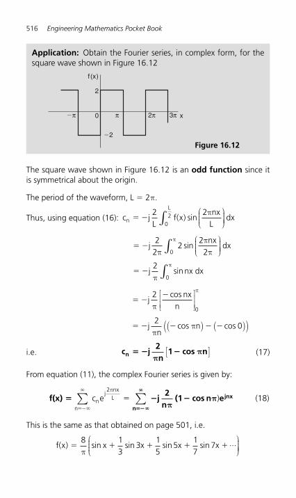
516 Engineering Mathematics Pocket Book
The square wave shown in Figure 16.12 is an odd function since it is symmetrical about the origin.
The period of the waveform, L � 2 π .
Thus, using equation (16): c jL
f xLn
L
� �2 2
02 ( ) sin
πnxdx
⎛⎝⎜⎜⎜
⎞⎠⎟⎟⎟⎟∫
� �
� �
j dx
j
22
222
2
0
0
ππ
π
π
π
π
sin
sin
nx
nx dx
⎛⎝⎜⎜⎜
⎞⎠⎟⎟⎟⎟∫
∫
� ��
� � � � �
jn
jn
n
2
20
0π
ππ
πcos
cos cos
nx⎡
⎣⎢⎢
⎤
⎦⎥⎥
( ) ( )( )
i.e. c j2n
1 cos nn � � �π
π[ ] (17)
From equation (11), the complex Fourier series is given by:
f(x) j2
n(1 cos n ejnx
n
� � ����
�
c enj
L
n
2πnx
���
�
∑ ∑�π
π) (18)
This is the same as that obtained on page 501, i.e.
f x x x x( ) sin sin sin sin� � � � �
8 13
315
517
7π
x ...⎛⎝⎜⎜⎜
⎞⎠⎟⎟⎟⎟
Application: Obtain the Fourier series, in complex form, for the square wave shown in Figure 16.12
Figure 16.12
0
�2
�π π 2π
2
3π
f (x)
x
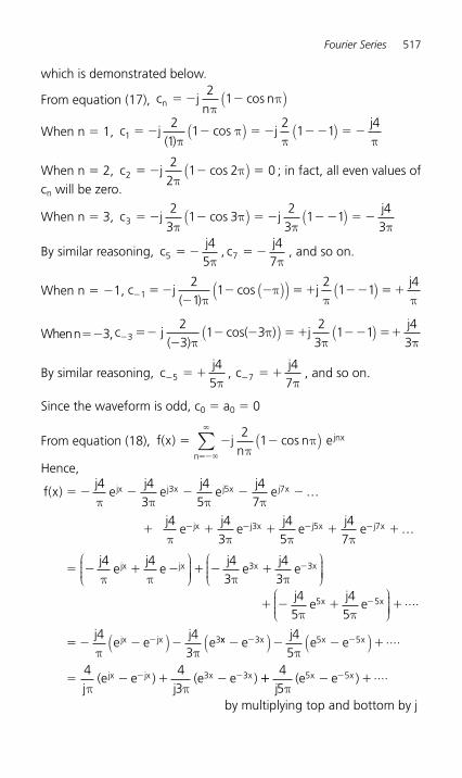
Fourier Series 517
which is demonstrated below.
From equation (17), c jn
nn � � �2
1π
πcos( )
When n � 1, c j jj
121
12
1 14
� � � � � � � � �( )
cosπ
ππ π
( ) ( )
When n � 2, c j22
21 2 0� � � �
ππcos( ) ; in fact, all even values of
cn will be zero.
When n � 3, c j jj
32
31 3
23
1 14
3� � � � � � � � �
ππ
π πcos( ) ( )
By similar reasoning, cj
cj
5 74
54
7� � � �
π π, , and so on.
When n � � 1, c j jj
� � ��
� � � � �� � �121
12
1 14
( )cos
ππ
π π( )( ) ( )
When n � � 3, c j jj
� ���
� � � � �� ��323
1 32
31 1
43( )
cos( )π
ππ π
( ) ( )
By similar reasoning, cj
cj
� �� � � �5 74
54
7π π, , and so on.
Since the waveform is odd, c 0 � a 0 � 0
From equation (18), f x jn
n en
jnx( ) cos� � ����
21
ππ( )∑
�
Hence,
f xj
ej
ej
ej
ejx j x j x j x( ) � � � � � �
4 43
45
47
3 5 7
π π π π…
� � � � �� � � �je
je
je
jejx j x j x j x4 4
34
54
73 5 7
π π π π…
� � � � � � �
�je
je
je
jejx jx x x4 4 4
34
33 3
π π π π
⎛⎝⎜⎜⎜
⎞⎠⎟⎟⎟⎟
⎛⎝⎜⎜⎜
⎞⎠⎟⎟⎟⎟
� � � �
� � � �
�
�
je
je
je e
je
x x
jx jx
45
45
4 43
5 5
3
π π
π π
⎛⎝⎜⎜⎜
⎞⎠⎟⎟⎟⎟
( )
....
xx x x x
jx jx x x
ej
e e
je e
je e
� � � �
� � � �
� �
� �
3 5 5
3 3
45
4 43
( ) ( )π
π π
....
( ) ( ) �� � ��45
5 5
je ex x
π( ) ....
by multiplying top and bottom by j
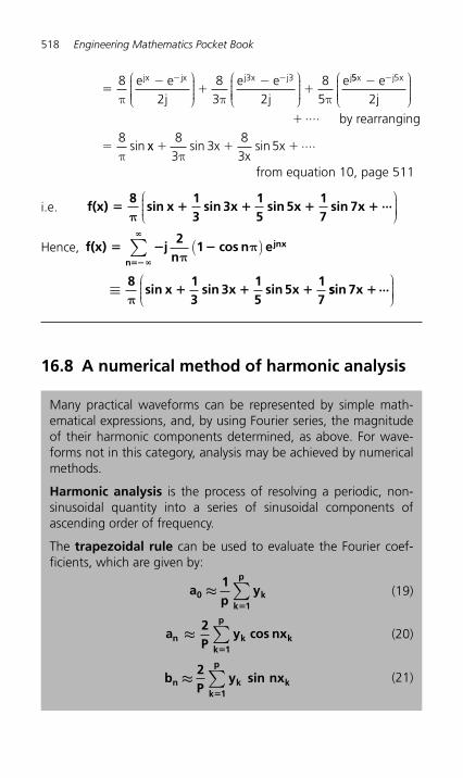
518 Engineering Mathematics Pocket Book
��
��
�� �8
283 2
85
3 3
π π πe e
je e
jejx jx j x j j⎛
⎝⎜⎜⎜⎜
⎞
⎠⎟⎟⎟⎟
⎛
⎝⎜⎜⎜⎜
⎞
⎠⎟⎟⎟⎟
55 5
2
x j xej
� �⎛
⎝⎜⎜⎜⎜
⎞
⎠⎟⎟⎟⎟
by rearranging�
�
....
sin8π
xx xx
x� � �83
383
5π
sin sin ....
from equation 10, page 511
i.e. f(x)8
sin x13
sin 3x15
sin 5x17
sin 7x� � � � �π
...⎛⎝⎜⎜⎜
⎞⎠⎟⎟⎟⎟
Hence, f(x) j2
n1 cos n e
8sin x
13
sin 3x15
sin 5x17
n
jnx� � �
� � �
���
�
ππ
≡π
( )∑
ssin 7x � ...⎛⎝⎜⎜⎜
⎞⎠⎟⎟⎟⎟
16.8 A numerical method of harmonic analysis
Many practical waveforms can be represented by simple math-ematical expressions, and, by using Fourier series, the magnitude of their harmonic components determined, as above. For wave-forms not in this category, analysis may be achieved by numerical methods.
Harmonic analysis is the process of resolving a periodic, non-sinusoidal quantity into a series of sinusoidal components of ascending order of frequency.
The trapezoidal rule can be used to evaluate the Fourier coef-ficients, which are given by:
ap
y0 kk 1
p
≈1
�∑ (19)
a
2P
y cos nxn kk 1
p
k≈�
∑ (20)
b
2P
y sin nxn k kk 1
p
≈�
∑ (21)
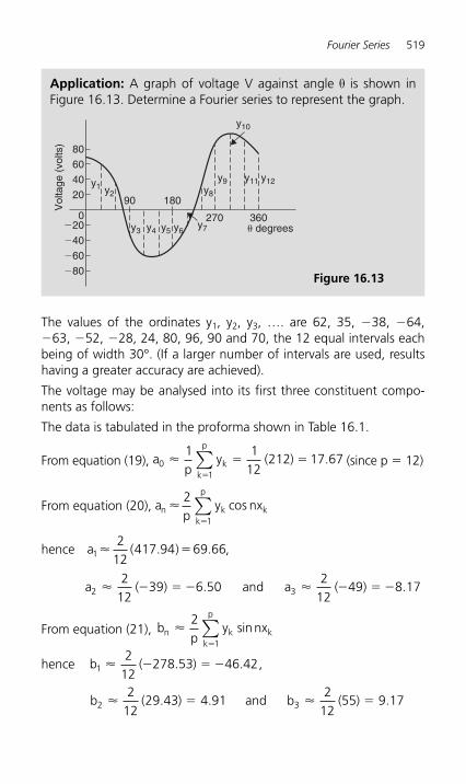
Fourier Series 519
The values of the ordinates y 1, y 2, y 3, …. are 62, 35, �38, � 64, �63, �52, �28, 24, 80, 96, 90 and 70, the 12 equal intervals each being of width 30°. (If a larger number of intervals are used, results having a greater accuracy are achieved).
The voltage may be analysed into its first three constituent compo-nents as follows:
The data is tabulated in the proforma shown in Table 16.1 .
From equation (19), a ykk
p
01
1 112
212 17 67�p �
� �∑ ( ) . (since p � 12)
From equation (20), a yn k kk
p
�2
1pnxcos
�
∑
hence a12
12417 94 69 66� ( . ) .� ,
a a2 3
212
39 6 502
1249 8 17� �( ) . ( ) .� � � � � �and
From equation (21), b y nxn k kk
p
�2
1psin
�
∑
hence b12
12278 53 46 42� ( . ) .� � � ,
b b2 3
212
29 43 4 912
1255 9 17� �( . ) . ( ) .� �and
Application: A graph of voltage V against angle θ is shown in Figure 16.13 . Determine a Fourier series to represent the graph.
80
Vol
tage
(vo
lts)
90 180
270 360� degrees
y1 y2
y3 y4 y5 y6
y8
y9 y11
y10
y7
y12
60
40
20
�20
�40
�60
�80
0
Figure 16.13
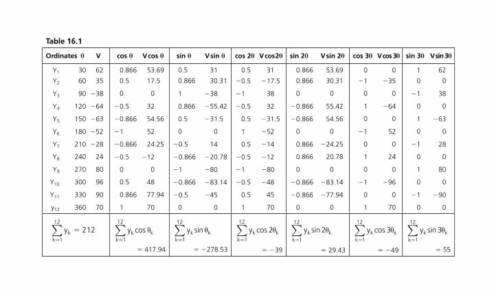
Table 16.1
Ordinates θ V cos θ V cos θ sin θ V sin θ cos 2 θ V cos 2 θ sin 2 θ V sin 2 θ cos 3 θ V cos 3 θ sin 3 θ V sin 3 θ
Y 1 30 62 0.866 53.69 0.5 31 0.5 31 0.866 53.69 0 0 1 62
Y 2 60 35 0.5 17.5 0.866 30.31 �0.5 �17.5 0.866 30.31 �1 �35 0 0
Y 3 90 �38 0 0 1 �38 �1 38 0 0 0 0 �1 38
Y 4 120 �64 �0.5 32 0.866 �55.42 �0.5 32 �0.866 55.42 1 �64 0 0
Y 5 150 �63 �0.866 54.56 0.5 �31.5 0.5 �31.5 �0.866 54.56 0 0 1 �63
Y 6 180 �52 �1 52 0 0 1 �52 0 0 �1 52 0 0
Y 7 210 �28 �0.866 24.25 �0.5 14 0.5 �14 0.866 �24.25 0 0 �1 28
Y 8 240 24 �0.5 �12 �0.866 �20.78 �0.5 �12 0.866 20.78 1 24 0 0
Y 9 270 80 0 0 �1 �80 �1 �80 0 0 0 0 1 80
Y 10 300 96 0.5 48 �0.866 �83.14 �0.5 �48 �0.866 �83.14 �1 �96 0 0
Y 11 330 90 0.866 77.94 �0.5 �45 0.5 45 �0.866 �77.94 0 0 �1 �90
y 12 360 70 1 70 0 0 1 70 0 0 1 70 0 0
ykk=∑
1
21
212�
y cosk kk
θ=
∑1
12
� 417.94
y sink k
k
θ=
∑1
12
� �278.53
y cosk k
k
21
12
θ=
∑
� �39
y sink kk
21
12
θ=
∑� 29.43
y cosk k
k
31
12
θ=
∑
� �49
y sink k
k
31
12
θ=
∑
� 55
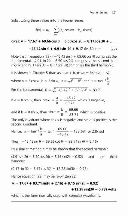
Fourier Series 521
Substituting these values into the Fourier series:
f x a a nx bn n
n
( ) ( cos sin )� � ��
01
nx�
∑
gives: v � 17.67 � 69.66 cos θ � 6.50 cos 2 θ � 8.17 cos 3 θ � …
� � � �46.42 sin 4.91sin 2 9.17 sin 3θ θ θ ... (22)
Note that in equation (22), ( �46.42 sin θ � 69.66 cos θ) comprises the fundamental, (4.91 sin 2 θ � 6.50 cos 2 θ) comprises the s econd har-monic and (9.17 sin 3 θ � 8.17 cos 3 θ) comprises the third harmonic.
It is shown in Chapter 5 that: a sin ω t � b cos ω t � R sin( ω t � α )
where a � R cos α , b � R sin α , R a b� �2 2 and α � tan � 1 ba
For the fundamental, R � � � �( . ) ( . ) .46 42 69 66 83 712 2
If a � R cos α , then cos.
.α � �
aR
−46 4283 71
which is negative,
and if b � R sin α , then sin..
� � �bR
69 6683 71
which is positive.
The only quadrant where cos α is negative and sin α is positive is the second quadrant.
Hence, � � ��
� �� �tan tan..
.1 1 69 6646 42
123 68ba
or 2.l6 rad
Thus, ( �46.42 sin θ � 69.66 cos θ ) � 83.71 sin( θ � 2.16)
By a similar method it may be shown that the second harmonic
(4.91 sin 2 θ � 6.50 cos 2 θ) � 8.15 sin(2 θ � 0.92) and the third harmonic
(9.17 sin 3 θ � 8.17 cos 3 θ ) � 12.28 sin(3 θ � 0.73)
Hence equation (22) may be re-written as:
v 17.67 83.71sin 2.16 8.15 sin(2 0.92)� � � � �
( )θ θ
� 12.28 siin(3 0.73) voltsθ � which is the form normally used with complex waveforms.
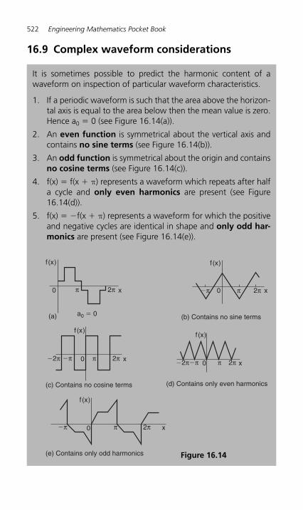
522 Engineering Mathematics Pocket Book
16.9 Complex waveform considerations
It is sometimes possible to predict the harmonic content of a waveform on inspection of particular waveform characteristics.
1. If a periodic waveform is such that the area above the horizon-tal axis is equal to the area below then the mean value is zero. Hence a 0 � 0 (see Figure 16.14(a) ).
2. An even function is symmetrical about the vertical axis and contains no sine terms (see Figure 16.14(b) ).
3. An odd function is symmetrical about the origin and contains no cosine terms (see Figure 16.14(c) ).
4. f(x) � f(x � π) represents a waveform which repeats after half a cycle and only even harmonics are present (see Figure 16.14(d) ).
5. f(x) � � f(x � π) represents a waveform for which the positive and negative cycles are identical in shape and only odd har-monics are present (see Figure 16.14(e) ).
0
(a) a0 � 0
π 2π
f (x)
x
(b) Contains no sine terms
0�π π
f (x)
2π x
(c) Contains no cosine terms
0�π π
f (x)
2π�2π x
(d) Contains only even harmonics
f(x)
0�π π 2π�2π x
(e) Contains only odd harmonics
0�π
f (x)
π 2π x
Figure 16.14
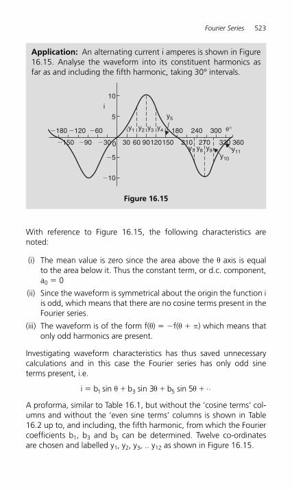
Fourier Series 523
With reference to Figure 16.15 , the following characteristics are noted:
(i) The mean value is zero since the area above the θ axis is equal to the area below it. Thus the constant term, or d.c. component, a0 � 0
(ii) Since the waveform is symmetrical about the origin the function i is odd, which means that there are no cosine terms present in the Fourier series.
(iii) The waveform is of the form f( θ ) � � f( θ � π) which means that only odd harmonics are present.
Investigating waveform characteristics has thus saved unnecessary calculations and in this case the Fourier series has only odd sine terms present, i.e.
i b b b� � � �1 3 53 5sin sin sin ..θ θ θ A proforma, similar to Table 16.1 , but without the ‘cosine terms ’ col-umns and without the ‘even sine terms ’ columns is shown in Table 16.2 up to, and including, the fifth harmonic, from which the Fourier coefficients b 1, b 3 and b 5 can be determined. Twelve co-ordinates are chosen and labelled y 1 , y 2 , y 3 , .. y 12 as shown in Figure 16.15 .
Application: An alternating current i amperes is shown in Figure 16.15 . Analyse the waveform into its constituent harmonics as far as and including the fifth harmonic, taking 30° intervals.
y1 y2 y3 y4
y5
i
�°
y7 y8 y9y10
y11
�10
�180 180 240 300�120 �60
�90 �30 30 60 90120150 210 270 330 360�150
�5
5
0
10
Figure 16.15
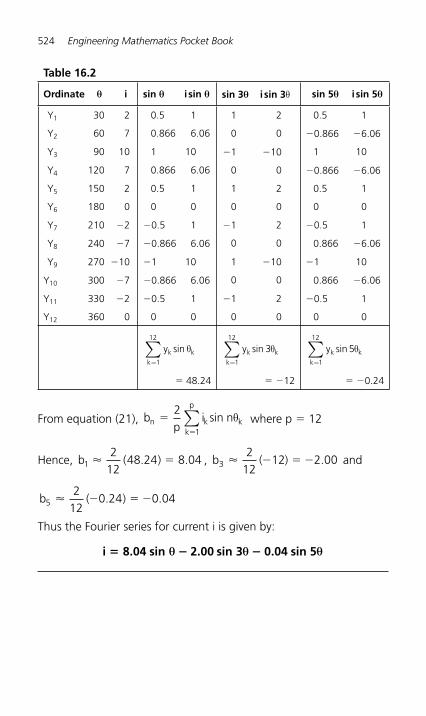
524 Engineering Mathematics Pocket Book
Table 16.2
Ordinate θ i sin θ i sin θ sin 3 θ i sin 3 θ sin 5 θ i sin 5 θ
Y 1 30 2 0.5 1 1 2 0.5 1
Y 2 60 7 0.866 6.06 0 0 �0.866 �6.06
Y 3 90 10 1 10 �1 �10 1 10
Y 4 120 7 0.866 6.06 0 0 �0.866 �6.06
Y 5 150 2 0.5 1 1 2 0.5 1
Y 6 180 0 0 0 0 0 0 0
Y 7 210 �2 �0.5 1 �1 2 �0.5 1
Y 8 240 �7 �0.866 6.06 0 0 0.866 �6.06
Y 9 270 �10 �1 10 1 �10 �1 10
Y 10 300 �7 �0.866 6.06 0 0 0.866 �6.06
Y 11 330 �2 �0.5 1 �1 2 �0.5 1
Y 12 360 0 0 0 0 0 0 0
yk k
k
sin θ=
∑1
12
� 48.24
yk k
k
sin 31
12
θ=
∑
� �12
yk k
k
sin 51
12
θ=
∑
� �0.24
From equation (21), bp
i nn k kk
p
��
2
1
sin θ∑ where p � 12
Hence, b12
1248 24 8 04� ( . ) .� , b3
212
12 2 00� ( ) .� � � and
b52
120 24 0 04� ( . ) .� � �
Thus the Fourier series for current i is given by:
i 8.04 sin 2.00 sin 3 0.04 sin 5� � �θ θ θ
Index
Acceleration , 265 Acute angle , 105 Adjoint of matrix , 221 Algebraic method of successive
approximations , 61 substitution, integration , 307
Alternate angles , 105 Amplitude , 129 And-function , 234 And-gate , 249 Angles of any magnitude , 125
elevation and depression , 113 Angle types , 105 Angstrom , 1 Angular measure , 2
velocity , 131 Applications of complex numbers ,
211 Arc length of circle , 77 , 79 Area, circle , 77
imperial , 1 metric , 1 of any triangle , 119 sector of circle , 77 , 80
Areas of irregular fi gures , 96 plane fi gures , 73 similar shapes , 76
Areas under and between curves , 336
Argument , 209 Arithmetic progressions , 36 Astroid , 273 Astronomical constants , 7 Asymptotes , 184 Average value of a waveform , 343
Bessel function , 402 Bessel’s equation , 402 Binary to decimal conversion , 65
hexadecimal conversion , 72 Binomial distribution , 434
series , 49 Bisection method , 59 Boolean algebra , 254
de Morgan’s laws , 241 Karnaugh maps , 242 laws and rules , 238
Cardioid , 177 , 273 Cartesian and polar co-ordinates , 116
form of complex number , 206 Catenary , 37 Centroids , 350 Chain rule , 261 Change of limits, integration , 309 Changing products of sines
and cosines into sums or differences , 146
sums or differences of sines and cosines into products , 147
Chi-square distribution , 454 Circle, arc length , 77
area of , 77 equation of , 81 sector of , 77
Circumference , 77 Coeffi cient of correlation , 443 Cofactor , 220 Combinational logic networks , 248 Combination of two periodic
functions , 197
526 Index
Complementary angles , 105 function , 379
Complex conjugate , 207 applications of , 211 equations , 206 , 207 numbers , 206
Complex or exponential form of a Fourier series , 511
Complex waveform considerations , 522
Compound angle formulae , 39 , 141 Compound angles , 141 Computer numbering systems , 65 Cone , 83 , 85 Confi dence levels , 448 Congruent triangles , 107 Constants, astronomical , 7
mathematical , 7 physical , 6
Continued fractions , 24 Continuous function , 180 Contour map , 297 Convergents , 24 Conversions , 1 Correlation, linear , 443 Corresponding angles , 105 Cosine rule , 119
waveform , 124 , 128 Cramer’s rule , 230 Cubic equations , 170 Cuboid , 82 Cumulative frequency distribution ,
421 , 423 curve , 421
Cylinder , 82 , 83 Cycloid , 273
Decile , 429 Decimal to binary conversion , 65
hexadecimal conversion , 71 via octal , 67
Defi nite integrals , 306 De Moivres theorem , 213 De Morgan’s laws , 241
Depression, angle of , 114 Derived units , 4 Determinants, 2 by , 2 , 218
3 by , 3 , 220 solution of simultaneous
equations , 226 Determination of law , 152
involving logarithms , 153 Differential calculus , 258
function of a function , 261 products and quotients , 259
Differential equations , 366
ad ydx
bdydx
cy2
20� � � , 375
ad ydx
bdydx
cy f x2
2� � � ( ) , 379
dydx
f x� ( ) , 366
dydx
f y� ( ) , 367
dydx
f x f y� ( ). ( ) , 368
dydx
Py Q� � , 373
numerical methods , 385
Pdydx
Q� , 371
using Laplace transforms , 483 Differentiation , 258
of hyperbolic functions , 263 implicit functions , 276 inverse hyperbolic functions ,
284 inverse trigonometric functions ,
281 , 282 logarithmic functions , 279 in parameters , 274 partial , 189 successive , 262
Direction cosines , 202 Discontinuous function , 180 Dividend , 20 Divisor , 20
Index 527
Dot product , 200 Double angles , 39 , 145
Elevation, angle of , 113 Ellipse , 73 , 178 , 273 Equation of a circle , 81 Equilateral triangle , 106 Euler’s method , 385 Euler-Cauchy method , 388 Evaluating trigonometric ratios , 110 Even function , 37 , 180 , 498 Exponential form of complex
numbers , 215 Fourier series , 511 functions , 31
Extrapolation , 151
Factor theorem , 21 Final value theorem , 478 Finite discontinuities , 180 Fourier cosine series , 498 Fourier series for non-periodic
function over period , 2 π , 496 Fourier series for periodic function
over period , 2 π , 492 Fourier series for periodic function
over period L , 504 Fourier sine series , 498 Fractional form of trigonometric
ratios , 112 Frequency , 131
distribution , 422 polygon , 420 , 422
Frobenius method , 398 Frustum of cone , 88
sphere , 92 Function of a function , 261
Gamma functions , 402 Gaussian elimination , 232 Geometric progressions , 47 Gradient of graph , 149 Graphical functions , 180 Graphs, cubic equations , 170
exponential functions , 31 hyperbolic functions , 37 logarithmic functions , 30 quadratic , 164 , 166 simultaneous equations , 163 straight line , 149 trigonometric functions , 124
Greek alphabet , 2 Grouped data , 420 , 426
Half range Fourier series , 501 , 508 Harmonic analysis , 518 Heat conduction equation , 411 Hectare , 1 Heptagon , 74 Hexadecimal number , 69
to binary conversion , 72 decimal conversion , 70
Hexagon , 74 , 75 Histogram , 420 , 422 , 428 Homogeneous fi rst order differential
equations , 371 Horizontal bar charts , 416 , 417 Hyperbola , 179 , 273
rectangular , 179 , 273 Hyperbolic functions , 36
differentiation of , 263 identities , 38 solving equations , 39
Imaginary part of complex number , 206
Implicit functions , 276 Infl exion, point of , 267 Initial value theorem , 477 Integral calculus , 303 Integrals, algebraic substitutions ,
307 defi nite , 306 by partial fractions , 317 by trigonometric and hyperbolic
substitutions , 310 standard , 303
Integration by parts , 323
528 Index
reduction formulae , 326
tan θ2
substitution , 319
Interior angles , 105 Interpolation , 150 Inverse functions , 182 , 281
3 by , 3 , 221 Laplace transforms , 480 of matrix, 2 by , 2 , 218 using partial fractions , 482
Inverse hyperbolic functions , 284 differentiation of , 285
Inverse trigonometric functions , 183
differentiation of , 281 Invert-gate , 249 Isosceles triangle , 106 Iterative methods , 58
Karnaugh maps , 242 Knot , 2
Lagging angle , 129 Laplace’s equation , 413 Laplace transforms , 472
inverse , 480 Laws of growth and decay , 33
logarithms , 28 , 279 Laws and rules of Boolean algebra ,
239 Leading angle , 129 Least-squares regression line , 445 Legendre’s equation , 403 Legendre’s polynomials , 404 Leibniz-Maclaurin method , 395 Leibniz’s theorem , 394 Length, imperial , 1
metric , 1 L’Hopital’s rule , 57 Limiting values , 57 Linear correlation , 443
fi rst order differential equations , 373
regression , 445 Litre , 1
Logarithmic scales , 158 differentiation , 279 forms of inverse hyperbolic
functions , 287 functions , 279
Logarithms , 28 , 153 Logic circuits , 248
gates , 248
Maclaurin’s theorem , 54 Mann-Whitney test , 464 Mass , 2 Mathematical constants , 5 , 6 , 7
symbols , 7 Matrices , 217
solution of simultaneous equations , 223
Maximum values , 102 , 267 , 295 Mean or average values, by
integration , 343 Mean value, of a waveform , 101
statistics , 424 , 426 Measures of central tendency , 424 Median , 424 Micron , 1 Mid-ordinate rule , 95
numerical integration , 331 Minimum value , 267 , 295 Minor of matrix , 220 Mode , 424 Modulus , 209
Nand-gate , 248 , 253 Napierian logarithms , 32 Newton-Raphson method , 63 Nor-gate , 248 , 253 Normal distribution , 437 Normals , 270 Nose-to-tail method , 189 Not-function , 234 Not-gate , 249 Numerical integration , 331
mid-ordinate rule , 331 Simpson’s rule , 332
Index 529
trapezoidal rule , 331 using Maclaurin’s series , 56
Numerical methods for fi rst order differential equations , 385
Numerical method of harmonic analysis , 518
Obtuse angle , 105 Octagon , 74 , 75 Octal , 68 Octal to binary and decimal , 68 Odd function , 37 , 181 , 498 Ogive , 421 , 424 Or-function , 234 Or-gate , 248
Pappus’s theorem , 354 Parabola , 273 Parametric equations , 273 Parallel axis theorem , 360
lines , 105 Parallelogram , 73
method for vector addition , 189 Partial differential equations , 405
differentiation , 289 fractions , 41 , 317 , 482
Particular integral , 379 solution of differential equation ,
375 Pentagon , 74 Percentage component bar chart ,
416 , 418 Percentile , 429 Period , 129 , 180 Periodic functions , 180 Perpendicular axis theorem , 360 Pictograms , 416 Pie diagram , 416 , 420 Point of infl exion , 267 Poisson distribution , 435 Polar co-ordinates , 115
curves , 171 form , 209
Polygons , 73
Polynomial division , 20 Power series for e x , 31
methods of solving differential equations , 394
Prefi xes , 5 Prismoidal rule , 99 Probability , 431 Product-moment formula , 443 Products and quotients , 259 Pyramid , 82 , 84 Pythagoras’s theorem , 108
Quadratic equations , 25 , 166 graphs , 164
Quadrilateral , 73 Quartiles , 429 Quotients , 24
Radian measure , 77 , 78 Rates of change using
differentiation , 264 partial differentiation , 293
Real part of complex number , 206 Reciprocal ratios , 110 Rectangle , 73 Rectangular form of complex
numbers , 206 hyperbola , 179 , 273 prism , 82 , 83
Recurrence relation , 396 Reduction formulae , 326 Refl ex angle , 105 Regression, linear , 445 Relationship between trigonometric
and hyperbolic functions , 139
Relative velocity , 195 Remainder theorem , 23 Resolution of vectors , 191 Right angle , 105 Right-angled triangle solution , 113 Rodrigue’s formula , 404 Root mean square values , 345 Runge-Kutta method , 390
530 Index
Saddle points , 296 Sampling and estimation theories ,
447 Scalar product of two vectors , 200
quantities , 188 Scalene triangle , 106 Second moments of area , 359 Sector of circle , 77 Semi-interquartile range , 430 Sign test , 457 Similar triangles , 107 Simpson’s rule , 96 , 98
numerical integration , 332 Simultaneous differential equations
by Laplace transforms , 487 Simultaneous equations, by Cramer’s
rule , 230 determinants , 226 Gaussian elimination , 232 graphical solution , 163 matrices , 223
Sine rule , 119 waveform , 102 , 124 , 127
Sinusoidal form A sin ( ωt φ ) , 131 SI units , 3 Small changes using differentiation ,
272 partial differentiation , 294
Solution of right-angled triangles , 113
Solving equations by algebraic method , 61
bisection method , 59 containing hyperbolic functions ,
39 iterative methods , 58 Newton-Raphson method , 63 quadratics , 25
Speed , 2 Sphere , 83 Standard derivatives , 258
deviation , 424 , 426 error of the means , 447 integrals , 303 Laplace transforms , 472
Stationary points , 267 Straight line graphs , 149 Student’s t distribution , 451 Successive differentiation , 262 Supplementary angles , 105 Surd form , 112 Symbols, acoustics , 14
atomic and nuclear physics , 17 electricity and magnetism , 13 light related electromagnetic
radiations , 14 mathematical , 7 mechanics , 11 molecular physics , 16 nuclear reactions and ionising
radiations , 19 periodic and related phenomena ,
11 physical chemistry , 15 quantities , 10 space and time , 10 thermodynamics , 12
Tally diagram , 421 Tangents , 270 Tangent waveform , 124
Tan θ2
substitution , 319
Theorem of Pappus , 354 Pythagoras , 108
Total differential , 292 Transpose of matrix , 221 Transversal , 105 Trapezium , 73 Trapezoidal rule , 95 , 518
numerical integration , 331 Triangle , 73 Triangles, properties of , 106 Trigonometric and hyperbolic
substitutions, integration , 310 Trigonometric ratios , 109
equations , 134 evaluating , 110 fractional and surd form of , 112 identities , 38 , 134
Index 531
Truth tables , 234 Turning points , 267
Ungrouped data , 416 Unit matrix , 219 Universal logic gate , 253
Vector addition , 189 products , 203 subtraction , 192
Vectors , 188 Velocity and acceleration, using
integration , 265 , Vertical bar chart , 416 , 418 Vertically opposite angles , 105
Volume , 1 Volumes and surface areas of frusta
of pyramids and cones , 88 irregular solids , 98 using Simpson’s rule , 96
Volumes of similar shapes , 87 solids of revolution , 347
Wave equation , 406 Wilcoxon signed-rank test , 460
Xor-gate , 250 Xnor-gate , 250
Zone of a sphere , 92