engineering presented on march 3, 2014
TRANSCRIPT


AN ABSTRACT OF THE THESIS OF
Storm J.C. Beck for the degree of Master of Science in Sustainable Forest Management and Civil
Engineering presented on March 3, 2014.
Title: The Use of LiDAR to Identify Forest Transportation Networks
Abstract approved:
John D. Sessions Katharine M. Hunter-Zaworski
The production of high value non-conventional products, such as long utility poles; or the
production of low value bulky products, such as chips or grindings; provide opportunities for
forest owners to increase value from their forests. The transport of these products requires the
use of specialized trucks and trailers. However, the lack of engineering records of forest roads
provides a challenging environment in the assessment of transportation of non-conventional
products. The primary challenge to transporting non-conventional products is determining if the
specialized vehicle can navigate the horizontal and vertical geometry, as well as turning around
near the landing.
LiDAR provides data that could aid in the evaluation of specialized vehicles at the
transportation network scale. In this thesis, a review of previous research using aerial and
terrestrial LiDAR to identify the forest transportation network is made. From this review it was
evident that few studies have tried to automatically extract forest road location. Hence, a process

to identify and extract forest roads from a LiDAR data was developed and implemented. The
two main principles that were used to identify forest roads were (1) intensity values change with
material properties and (2) ground point densities differ on forest roads compared with the forest
floor. These two principles are used in conjunction with buffering, removing, and connection
routines. The removing and connection routines work to remove short isolated road segments
and to connect segmented road segments.
The road extraction process identified 67 percent of the roads that were field sampled. If gravel
and native surface roads were separated from the analysis, the process identified 84 percent of
the gravel and 10 percent of the dirt forest road segments by length. When assessing results of
the road extraction process across the entire area stratified by canopy cover, the results were 80
percent true positives, 34 percent false positives, 20 percent false negative, 38 percent true
negatives.
Finally the road geometry of the aerial LiDAR data were compared to terrestrial LiDAR data.
This comparison focused on the following attributes, road width, cross-slope, left cut/fill slope,
right cut/fill slope. The average absolute difference in the road width between the two methods
was 1.1m, the cut/fill slope differences was less than four percent, and the difference in road
cross slope was two percent. These results are comparable to other published results.
Future research and additions to this road identification and extraction process include adding an
image analysis process to help identify roaded areas and eliminate large areas of non-roaded area
as identified in the first process. After the road identification process a thinning algorithm could

be used to identify the road centerline providing vehicle paths throughout the transportation
network. These paths and a 3-D model of the forest road could be used in a vehicle conflict
analysis. Finally, a vehicle conflict analysis could provide a vehicle accessibility and product
production map of the forest providing economic, environmental, and societal benefits.

© Copyright by Storm J.C. Beck
March 3, 2014
All Rights Reserved

The Use of LiDAR to Identify Forest Transportation Networks
by
Storm J.C. Beck
A THESIS
submitted to
Oregon State University
in partial fulfillment of
the requirements for the
degree of
Master of Science
Presented March 3, 2014
Commencement June 2014

Master of Science thesis of Storm J.C. Beck presented on March 3, 2014.
APPROVED:
Co-Major Professor, representing Sustainable Forest Management
Co-Major Professor, representing Civil Engineering
Head of the Department of Forest Engineering, Resources and Management
Head of the School of Civil and Construction Engineering
Dean of the Graduate School
I understand that my thesis will become part of the permanent collection of Oregon State
University libraries. My signature below authorizes release of my thesis to any reader upon
request.
Storm J.C. Beck, Author

ACKNOWLEDGEMENTS
I would like to thank Leica Geosystems for providing OSU with Cyclone licenses.

CONTRIBUTION OF AUTHORS
I would like to thank Dr. John Sessions, Dr. Kate Hunter-Zaworski, Dr. Michael Olsen, Dr.
Michael Wing, Dr. Kevin Boston, and Dr. David Myrold for their continuing support and
encouragement throughout this entire process.

TABLE OF CONTENTS
Page
Chapter 1 - Introduction .................................................................................................................. 1
1.1 - Organization ........................................................................................................................ 3
1.2 - Literature Cited ................................................................................................................... 3
Chapter 2 - LiDAR and Remote Sensing ........................................................................................ 5
2.1 - Classifying Returns ............................................................................................................. 7
2.2 - Intensity of Returns ............................................................................................................. 9
2.3 - Literature Cited ................................................................................................................. 10
Chapter 3 - Road Extraction from LiDAR Data Sets ................................................................... 13
3.1 Discussion ........................................................................................................................... 19
3.2 - Literature Cited ................................................................................................................. 19
Chapter 4 - Registration of Terrestrial LiDAR Data Sets ............................................................. 21
4.1 - Background ....................................................................................................................... 21
4.1.1 - Study Area .................................................................................................................. 21
4.1.2 - Datasets ...................................................................................................................... 21
4.1.3 - Naming Convention ................................................................................................... 22
4.2 - Methodology ..................................................................................................................... 23
4.2.1 - Data Collection ........................................................................................................... 23
4.2.2 - Registration ................................................................................................................ 32
4.3 - Results ............................................................................................................................... 34
4.3.1 - Data Collection ........................................................................................................... 34
4.3.2 - Registration ................................................................................................................ 35
4.4 – Comparison ...................................................................................................................... 41
4.4.1 - Registration ................................................................................................................ 41
4.5 - Discussion ......................................................................................................................... 42
4.5.1 - Potential Problems...................................................................................................... 42
4.6 - Conclusion ........................................................................................................................ 45

TABLE OF CONTENTS (Continued)
Page
4.7 - Literature Cited ................................................................................................................. 46
Chapter 5 - Forest Road Geometry Extraction and Comparison .................................................. 47
5.1 - Abstract ............................................................................................................................. 47
5.2 - Introduction ....................................................................................................................... 48
5.3 - Background ....................................................................................................................... 49
5.4 - Methods............................................................................................................................. 50
5.4.1 - Extraction form Aerial LiDAR Data Sets .................................................................. 50
5.4.2 - Terrestrial LiDAR Data Collection ............................................................................ 60
5.4.3 - Statistically Filtering Terrestrial LiDAR Data Sets ................................................... 61
5.4.4 - Road Geometry Extraction ......................................................................................... 64
5.5 - Results ............................................................................................................................... 66
5.5.1 - Road Extraction form Aerial LiDAR Data ................................................................ 66
5.5.2 - Road Geometry Comparison ...................................................................................... 71
5.6 - Conclusion ........................................................................................................................ 74
5.7 - Literature Cited ................................................................................................................. 75
Chapter 6 - Conclusion and Future Research ............................................................................... 76
6.1 - Future Research Areas ...................................................................................................... 76
6.2 - Quality Assessment ........................................................................................................... 79
6.2.1 - Effect of Vehicle Type on Needed Data Quality ....................................................... 79
6.2.2 - Comparison of LiDAR Results to Conventional Field Equipment ............................ 79
6.3 - 3-D Vehicle Analysis ........................................................................................................ 80
6.4 - Potential Benefits .............................................................................................................. 83
6.5 - Literature Cited ................................................................................................................. 85
Appendix A ................................................................................................................................... 86
Appendix B ................................................................................................................................... 97
Appendix C ................................................................................................................................. 107

TABLE OF CONTENTS (Continued)
Page
Appendix D ................................................................................................................................. 116

LIST OF FIGURES
Figure Page
Figure 2.1. LiDAR Footprint and Returns (Nolin, 2011). ............................................................. 6
Figure 2.2. Intensity image of a forested area. The image is colored by intensity values, dark
indicating low intensity values and light being high intensity values. ........................................... 7
Figure 3.1. Road edges using standard edge extraction techniques (Rieger et al. 1999)............. 14
Figure 3.2. Road edges after the used of snakes bridging gaps and smoothing road edges (Rieger
et al. 1999). ................................................................................................................................... 15
Figure 3.3. Hand digitized road centerline using a one meter DEM (White et al., 2010). .......... 17
Figure 4.1. FARO FOCUS3D terrestrial laser scanner. ................................................................ 24
Figure 4.2. 152.4 mm diameter spherical target. ......................................................................... 25
Figure 4.3. Sphere and scanner location within a point cloud. The red diamonds are the target
locations and the red pentagons are the scanner locations. ........................................................... 25
Figure 4.4. Sphere and scanner location on a road segment ......................................................... 26
Figure 4.5. A close up image of the scanner and target setup at a middle control point. ............ 27
Figure 4.6. A map of the control points for the terrestrial scan, total station setup locations, and
static GPS observations................................................................................................................. 28
Figure 4.7. Topcon HiperLite+ GPS Unit. ................................................................................... 29
Figure 4.8. Naming convention used during the second registration process. ............................ 33
Figure 4.9. A road sample colored by scan position. ................................................................... 39
Figure 4.10. A close up view of a few trees showing the blending of the individual scans. ....... 40
Figure 4.11. A cross-section of a tree trunk. ................................................................................ 40

LIST OF FIGURES (Continued)
Figure Page
Figure 4.12. Saturation (cone of points) and target shift away from scanner (center of sphere vs
center of pole). .............................................................................................................................. 44
Figure 4.13. Misalignment of sphere targets in registration process ........................................... 45
Figure 5.1. Intensity return map of a forested area in the McDonald Forest. The image is
colored by intensity values, dark indicating low intensity values and light indicating high
intensity values.............................................................................................................................. 52
Figure 5.2. The second step in identifying an acceptable intensity value ranges for each cover
type. The red circles indicate the ranges in which a majority of the points fall within, this is
where a fine tuning of the ranges started. ..................................................................................... 54
Figure 5.3. The third step in the preprocessing steps of selecting appropriate intensity value
ranges for various canopy types. ................................................................................................... 54
Figure 5.4. An illustration of the high ground return density along a forest road compared to the
surrounding forest floor. ............................................................................................................... 56
Figure 5.5. An example of the isolated and connection routines. Cells with an “O” will be
removed after the isolation routine and the cells with an “A” will be added after the connection
routine. .......................................................................................................................................... 57
Figure 5.6 The workflow for the road extraction process. RL = roaded list, imin=minimum
acceptable intensity value, imax= maximum acceptable intensity value ADJ=adjacent, DTelv =
Delaunay Triangulation, GRIDRL= road list of the grid, csize=cell size, mgrade= maximum road
grade, mindist = minimum distance, {RL} = set of points in the road list, {N} = set of all ground
points, {GRID}= set of cells within the grid of the area, {ZADJ}=set of cells that are adjacent to
cell Z, {w}{p} = set of cells that connected to cell w, wpyc = the y coordinate of the center of the
cell connected to cell w, pz = the average elevation of cell p, -> = place into set ........................ 59
Figure 5.7. Typical forest road cross-section for a cut and fill section. ....................................... 62
Figure 5.8. The extracted transect from the road sample 400 Y G Y. ......................................... 65
LIST OF FIGURES (Continued)
Figure Page
Figure 5.9. The identified roaded areas of the forest road extraction process for a young canopy
cover and a maximum road grade of 20 percent. The young canopy cover is found in the center
of the image, producing minimal gaps in road identification. The gaps increase due to the
differing canopy covers................................................................................................................. 66
Figure 5.10. (A) The areas identified as roaded using the road extraction process for a mature
cover type with a 10 percent maximum road grade. (B) The terrestrial road segment 400 O G N
(upper right corner of the image) that was of interest when running the road extraction process
shown in (A). ................................................................................................................................ 68
Figure 5.11 (A) Transects of the 400 Y G Y road segment. Overlapping transects are desired; as
transects at 90 degrees to the road centerline capture the desired road geometry for evaluating
vehicle accessibility. (B) A extracted road cross-sections in A (red arrow). Notice the smooth
aerial data and the fine terrestrial data. ......................................................................................... 72
Figure 5.12. A road profile from road segment 410 O D Y. Notice the spikes in the terrestrial
data, this is the result of using the statistical vegetation filter in a heavily grassed location. ....... 73
Figure 6.1. An example of a large continuous section of non-roaded area. ................................ 77
Figure 6.2. Potential challenges with image analysis to identify forest roads. ............................ 78
Figure 6.3. Standard 2-D evaluation of vehicle accessibility. (U.S. Department of
Transportation, 2012) .................................................................................................................... 81
Figure 6.4. A 3-D model of the forest transportation network, in which conflict analyses could
be performed with different vehicles. ........................................................................................... 82
Figure 6.5. The benefit of a 3-D evaluation of non-standard vehicle accessibility. Notice how
the poles manage to skim atop of the cut-slope. (Ken Montgomery Trucking Inc., McMinnville
City Watershed, Oregon) .............................................................................................................. 83
Figure 6.6. A simplified example of a multiple rotation aged forest, incorporating vehicle
accessibility and economical returns. ........................................................................................... 84
Figure D.1. Wheelbase Definition for a Log Truck with Stinger-Steered Trailer (Erkert T.W.,
Sessions, Layton, and Bell, 1989). .............................................................................................. 118

LIST OF TABLES
Table Page
Table 4.1. Road sample naming convention. ............................................................................... 23
Table 4.2. Tolerances of surveys. ................................................................................................ 30
Table 4.3. Static GPS observation results, all measurements are in meters. ............................... 31
Table 4.4. The number of points per scan location and road sample. .......................................... 35
Table 4.5. Fit statistics for the control spherical targets for the Register-then-Transform process.
....................................................................................................................................................... 36
Table 4.6. Errors using Register-then-Transform. (MF- manual fit, no errors were computed) . 37
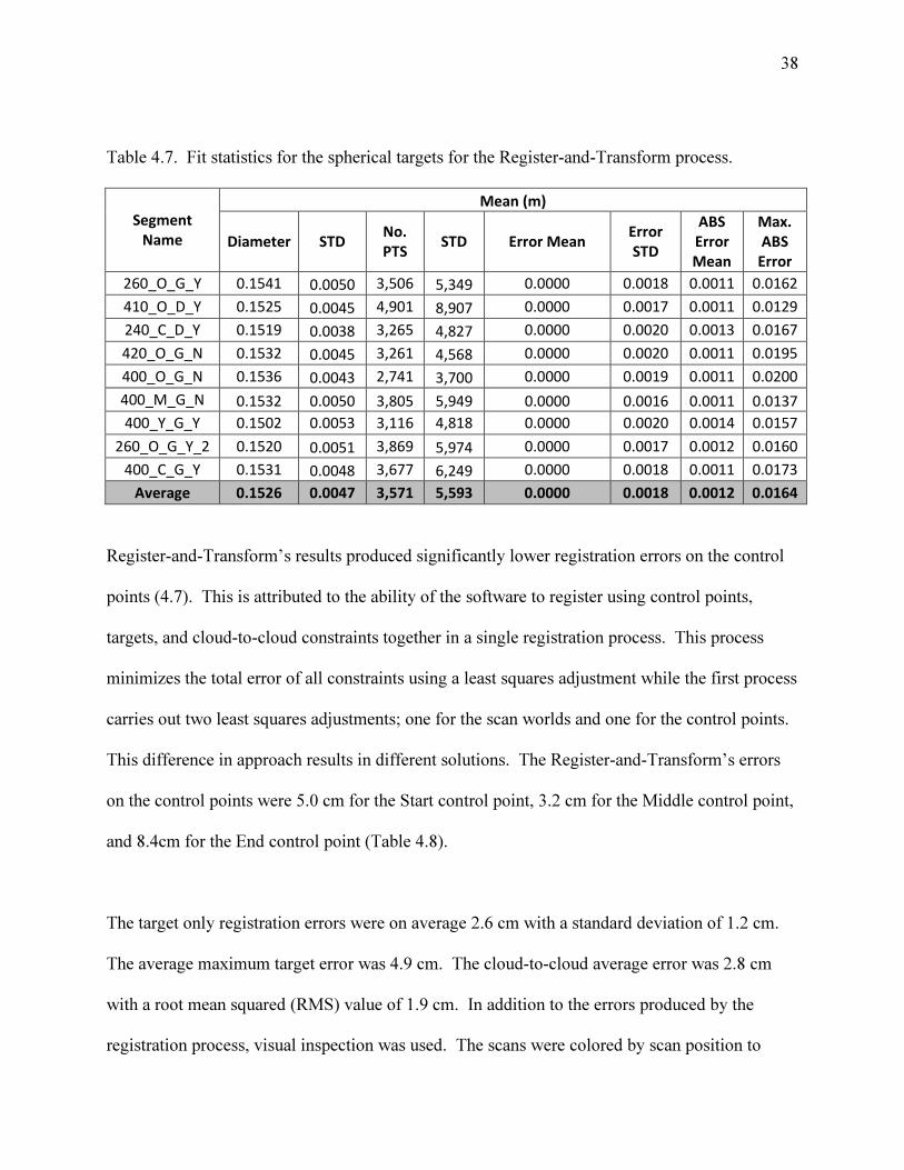
Table 4.7. Fit statistics for the spherical targets for the Register-and-Transform process. ......... 38
Table 4.8. Errors using Register-and-Transform. ........................................................................ 39
Table 4.9. Differences in registration errors of control points between Register-then-Transform
and Register-and-Transform. ........................................................................................................ 41
Table 5.1. The determined intensity value ranges for identifying roaded areas. ......................... 55
Table 5.2. The road extraction results compared to the field measured road segments (sorted by
surface type than by covertype) .................................................................................................... 67
Table 5.3. Road extraction statistics for the entire study area. These statistics are biased by
including all cover types not just the cover type of interest. ........................................................ 69
Table 5.4. Road extraction statistics for only cover types of interest. ......................................... 70
Table 5.5. The summary table of the difference between the extracted road geometry variables.
All measurements are in meters. ................................................................................................... 74
Table D.1. Vehicle Configurations, L3 is an estimate of the extended reach (all measurements
are in meters)............................................................................................................................... 117

LIST OF TABLES (Continued)
Table Page
Table D.2. Minimum lane widths from various off-tracking determination methods (all
measurements are in meters). ...................................................................................................... 118
Table D.3. Statistics for the minimum lane widths (all measurements are in meters). ............. 119

The Use of LiDAR to Identify Forest Transportation Networks
Chapter 1 - Introduction
Non-conventional products such as long utility poles or bulky products such as chips provide
opportunities for forest owners to increase value from their forests. However, as Sessions et al.
(2010) states, "most of the forest transportation system has been designed and built for long-log,
stinger-steered trailers" and as Craven (2011) reports, "there is little engineering record of road
design or location throughout the forest industry." Lysne and Klumph (2011) and Beathe (2011)
also provide similar statements. Unfortunately, the 6,070 hectare OSU College Forests and the
28,330 hectare Starker Forests have no data on the horizontal, vertical, or cross-sections of their
roads (Lysne and Klumph, 2011 and Beathe, 2011). This lack of engineering records provides a
challenging environment for the assessment of transporting non-conventional products. The
primary challenge to hauling non-conventional products, on non-standard vehicles, is
determining if the vehicle can navigate the horizontal and vertical geometry loaded, as well as
turning around unloaded.
Currently, two methods are used in practice to determine if specialized vehicles can navigate the
road system: contractor visual inspection and field measurements (Lysne and Klumph, 2011 and
Beathe, 2011). According to Lysne and Klumph (2011) and Beathe (2011), the College
Research Forests and Starker Forests will have the contractor of the non-conventional products
look over the roads and evaluate what types of vehicles can navigate from the product pickup
point in the forest (landing) to the highway. With this approach, only segments of the road

2
network are analyzed for a certain type of vehicle, leaving a large gap in knowledge about the
accessibility of specialized vehicles throughout the road network. The second approach to
determine vehicle accessibility is field measurements of road width and radius around critical
curves. The coefficient of traction and vertical curve geometry can also be obtained in the field
assessment. Not only are these field measurements time consuming, but they only provide a
snap shot of the accessibility of the transportation network (Sessions et al., 2010).
A network analysis to assess vehicle accessibility of the horizontal geometry of the
transportation network would provide detailed information about the transportation infrastructure
when evaluating product potential. The emerging technology of Light Detection and Ranging,
LiDAR, suggests it can provide an opportunity to aid in evaluating the accessibility of non-
conventional forest products on the horizontal geometry, throughout an ownership. A vehicle
accessibility map of the horizontal geometry would provide landowners with the knowledge of
what high valued forest products (poles) or bulky low value forest products (chips or hog fuel)
can be transported from the forests on what types of vehicles. This map alone, will not be
sufficient to aid landowners in determining if the vehicle can negotiate the vertical geometry or
turnaround. Field measurements and proper landing design will still be required to assure that
the vehicle can navigate the vertical geometry and turn around safely at or near the landing.
This thesis focuses on road extraction from LiDAR data sets. The contribution of this work is an
algorithm that considers intensity and point density information to identify forest roads. It was
theorized that gravel and native surface roads could be identified using these parameters in aerial
LiDAR data. This hypothesis, as explained in more detail later, was tested by collecting a

3
subsample of road geometries using terrestrial LiDAR and comparing them to extracted road
geometries from aerial LiDAR data sets. The field collected data was collected to focus on the
best and worst case road extraction potential, providing the opportunity to identify the limits of
the technology.
1.1 - Organization
This thesis is organized into six chapters. Chapter 1 serves as an introduction to the thesis.
Chapter 2 provides background information on Light Detection and Ranging (LiDAR) and
remote sensing. Chapter 3 discusses previous research in extracting forest road geometry from
LiDAR data. Chapter 4 provides the field data collection process along with a discussion on
methods employed to post process the field data. Chapter 5 is a manuscript chapter, describing
the road extraction process and presenting results of implementation. Chapter 6 concludes the
entire thesis and suggests future research and applications.
1.2 - Literature Cited
Beathe, J. (2011, December 21). Starker Forests' Road Inventory. (S. Beck, Interviewer)
Corvallis, Oregon.
Craven, M., Wing, M., Sessions, J., & Wimer, J. (2011). Assessment of Airborne Light Detection
and Ranging (LiDAR) for use in Common Forest Engineering Geomatic Applications.
M.S. Thesis, Oregon State Universtiy, College of Forestry, Corvallis. Retrieved from
Oregon State University: http://hdl.handle.net/1957/21803

4
Lysne, D., & Klumph, B. (2011, December 14). OSU College Forests' Road Inventory. (S. Beck,
Interviewer) Corvallis, Oregon.
Sessions, J., Wimer, J., Costales, F., & Wing, M. G. (2010). Engineering Considerations in Road
Assessment for Biomass Operations in Steep Terrain. Western Journal of Applied
Forestry, 25(3), 144-153.

Chapter 2 - LiDAR and Remote Sensing
LiDAR is an active remote sensing technology. An active remote sensing technology produces
its own energy that is transmitted toward the study area and interacts with the study area creating
a backscatter of energy that is recorded by the sensor. This can be compared to a passive sensing
technology that relies on the energy that is reflected or emitted from the Earth's surface and
atmosphere (Jenson, 2007).
The process of aerial LiDAR data collection involves three main components: a laser scanner, a
global positioning system, GPS, and an inertial measurement unit, IMU (Renslow, 2012). The
laser scanner is used to determine range using pulses of light (laser light emitted from the laser
scanner). The GPS is used to determine the aircrafts position (X, Y, and Z) and the IMU is used
to correct the GPS positioning data based on the aircraft’s yaw, pitch, and roll. Depending on the
range height of the aircraft (the elevation above the study area) the footprint of the pulse will
vary. It is typically 1/1000 of the range height (e.g. 0.75 m footprint for a 750 m range height)
(Baltsavias, 1999). Several objects may lie within a laser’s footprint and thus part of the laser
energy will reflect off the first object encountered, while the remaining energy will continue to
the ground interacting with objects it encounters until it backscatters with the ground (Figure
2.1). A return is a portion of the pulse that is backscattered from the study area and received by
the laser scanner. The returns are classified as first, second, etc. according to the order, which the
scanner receives them (Figure 2.1). The GPS unit is used to constantly record the aircraft's
position. The IMU is used to collect the aircraft's yaw, pitch, and roll, Y, X, and Z positions. The

6
yaw, pitch, and roll of the aircraft are used to correct the scanner data to account for the inability
of the aircraft to fly perfectly level (Craven et al., 2011 and Jenson, 2007).
Figure 2.1. LiDAR Footprint and Returns (Nolin, 2011).
LiDAR also measures the intensity of the returns, which is defined as the amount of energy
backscattered from the study area. Many factors affect the intensity levels including material
properties, range, angle of incidence, and atmospheric dispersion. Intensity values varying
depending on the material, which can aid in the identification of features, as shown in Figure 2.2
(Jenson, 2007).

7
Figure 2.2. Intensity image of a forested area. The image is colored by intensity values, dark
indicating low intensity values and light being high intensity values.
2.1 - Classifying Returns
Classification algorithms are an area of current research interest. Saito et al. (2009) identified
that the LiDAR data had a large amount of vertical error, 0.33m in the open and 1.5m in the
forest. To alleviate this problem they used a new technique, developed by Saito et al. (2008)
which produced geographical features more clearly than the 1m grid digital elevation model,
DEM. White et al. (2010) identified that ground point classification performed by TerrascanTM
created gaps in the ground point coverage, especially along the road edges. To alleviate gaps in
the ground point coverage White et al. (2010) used the method established by Evans and Hudak
(2007) to reclassify ground returns, which increased the number of ground returns by 17.5%.

8
As both of these articles indicate, the way the returns are classified can have a large impact on
the accuracy of the surface model. Meng, Currit, and Zhao (2010) reviewed several ground
filtering algorithms and discussed several critical issues that these algorithms face. Meng, Currit,
and Zhao (2010) state, "ground filtering algorithms perform best when specific surface
conditions are met." This statement clearly identifies why Saito et al. (2009) and White et al.
(2010) encountered problems; their ground filtering algorithms were not suited for the terrain
and vegetation. This clearly identifies that the selection of a ground classification algorithm is
extremely important to the quality of the surface model.
Meng, Currit, and Zhao (2010) classified ground classification algorithms into six categories.
The classifications are segmentation/cluster, morphology, directional scanning, contour,
triangulated irregular network (TIN), and interpolation. The following paragraphs will highlight
the processes and advantages of directional scanning, TIN, and interpolation classifications.
Directional scanning is a "method to remove non-ground points based on slope and elevation
difference calculated along the scan line" (Meng, Currit, & Zhao, 2010). However, this method
is sometimes sensitive to sudden ground changes; to overcome this problem a multi-directional
ground-filtering algorithm was created. This method combines directional scanning and two-
dimensional kernel-based methodology; preserving objects shapes and its sensitivity to low
vegetation (Meng, Currit, and Zhao, 2010).
TIN-based filters removes non-ground points based on the smoothness of the ground. This
assumes that the ground is smooth and free from sharp corners. This method employs an

9
iterative TIN creation method. It first creates a TIN, determines the points with strong curvature,
deletes them from the TIN, and repeats this process until no points are left with strong curvature.
However, large buildings and low buildings are not typically removed using this process.
Axelsson (1999) developed an active-TIN method, which gradually removes non-ground points
based on the elevation difference and angle to the closest triangle. Fifteen experiments have
shown that Axelsson's method presents the best performance in terms of average overall
accuracy (Meng, Currit, and Zhao, 2010).
Interpolation based methods compare the elevation of points with estimated values with
interpolation algorithms. A method based on "linear least-square interpolation with a set of
adaptive weight functions" was successfully tested in forested areas (Meng, Currit, and Zhao,
2010). Evans and Hudak used the thin plate spline method with a changing interpolation cell
size (Evans and Hudak, 2007). This showed improvement in removing understory vegetation
and White et al. (2010) claimed an increased the number of ground returns by 17.5% over
TerrascanTM.
Overall, the ground classifying method used will dictate the starting quality of the solution. Each
method discussed has strengths and weakness and are designed for specific environments. Great
care must be taken when selecting a ground classifying method; the filter is calibrated to a
specific terrain type.
2.2 - Intensity of Returns

10
As with classifying returns, great care must be taken when using intensity returns for object
identification. As mentioned earlier intensity return levels very with material properties, range,
angle of incidence, and atmospheric dispersion (Jenson, 2007). While the intensity value will
vary depending on material properties, the same material will produce varying levels of intensity
based on range, angle of incidence, and atmospheric dispersion. To account for these variables
and to help identify objects, intensity values should be normalized.
Höfle and Pfeifer (2007) developed two methods to normalize intensity values, (1) data driven
and (2) model driven. The first method is based on multiple flying altitudes for a section of the
scanned area. The first method relays on the assumption that a majority of the returns are single
returns not multiple returns. This assumption is not valid in forested environments where
multiple returns are the normal situation. The second method is based on the recorded intensity
values being "proportional to the ground reflectance and to the flying height" (Höfle and Pfeifer,
2007). The second method requires multiple flying heights over a homogenous area to estimate
the coefficients of the relationship and then can be applied to the entire study area. Both of these
approaches significantly reduced intensity variation over the study area. The authors conclude
that the model driven approach is preferred due to no special requirements on the design of the
flight plan.
2.3 - Literature Cited
Axelsson, P. (1999). Processing of laser scanner data—algorithms and applications. ISPRS
Journal of Photogramemetry & Remote Sensing, 54, 138-147.
Baltsavias, E. P. (1999). Airborne Laser Scanning: Basic Relations and Formulas. Journal of
Photogrammetry & Remote Sensing, 54, 199-214.

11
Craven, M., Wing, M., Session, J., and Wimer, J. (2011). Assessment of Airborne Light
Detection and Ranging (LiDAR) for use in Common Forest Engineering Geomatic
Applications. M.S. Thesis, Oregon State Universtiy, College of Forestry, Corvallis.
Retrieved from Oregon State University: http://hdl.handle.net/1957/21803
Renslow, M. (Ed.). (2012). Airborne Topographic LiDAR Manual. (1st ed.). ASRPS.
Evans, J. S., and Hudak, T. (2007). A multiscale curvature algorithm for classifying discrete
return LiDAR in Forested Environments. IEEETransactions on Geoscience and Remote
Sensing, 45, 1029-1038.
Höfle, B., and Pfeifer, N. (2007). Correction of Laser Scanning Intensity Data: Data and Model-
Drivern Approaches. ISPRS Journal of Photogrammetry & Remote Sensing, 62, 415-433.
Jenson, J. R. (2007). Remote Sensing of the Environment: An Earth Resource Perspective. (J.
Howard, D. Kaveney, K. Schiaparelli, and E. Thomas, Eds.) Upper Saddle River, NJ:
Pearson Prentice Hall.
Meng, X., Currit, N., and Zhao, K. (2010). Ground Filtering Algorithms for Airborne LiDAR
Data: A Review of Critical Issues. Remote Sensing(2), 833-860. doi:10.3390/rs2030833
Nolin, A. (2011, November). Remote Sensing of the Environment Class Notes. Corvallis,
Oregon: Department of Geosciences, Oregon State University.
Saito, M., Aruga, K., Matsue, K., Tasaka, T. (2008). Development of the Filtering Technique of
the Intersection Angle Method using LiDAR data of the Funyu Experimental Forest.
Journal of the Japan Forestry Engineering 22 (4).
Saito, Masashi, Masahiro Goshima, Kazuhiro Aruga, Keigo Matsue, Yasuhiro Shuin, and
Toshiaki Tasaka. "The Study of the Automatic Forset Road Design Technique
Considering Shallow Landslides with LiDAR Data of the Funyu Experimental Forest."

12
Council on Forest Engineering (COFE) Conference Proceedings: “Environmentally
Sound Forest Operations.”. Lake Tahoe, 2009. 1-12.
White, R. A., Dietterick, B. C., Mastin, T., and Strohman, R. (2010). Forest Roads Mapped
Using LiDAR in Steep Forested Terrain. Remote Sensing, 2(4), 1120-1141.

Chapter 3 - Road Extraction from LiDAR Data Sets
Mapping forest roads using LiDAR data is an evolving process. Rieger et al. (1999), White et al.
(2010) and Craven et al. (2011) have mapped forest roads using LiDAR through various
techniques. These techniques include standard edge extraction, hand digitization, and hand
digitization with a script to adjust the hand digitization centerline, these techniques have been
used on small scales.
Rieger et al. (1999) approached mapping forest roads to create break lines for more accurate
digital terrain model (DTM) creation. The roads were mapped using a hill-shaded map and
standard edge extraction techniques of the area (Figure 3.1). The road edges were then enhanced
using a sigma filter, which is an edge preserving and edge enhancing smoothing filter. With the
road edges, enhanced line features were extracted based on the Forstner Operator. The Forstner
Operator is based on the first derivative of the grey levels; applying thresholds can classify each
pixel as belonging to either a homogeneous region, a region containing a line (specifically for
break line detection), or a heterogeneous region. The results of the Forstner Operator must be
thinned out to exclude irrelevant lines and then approximated by polygons.

14
Figure 3.1. Road edges using standard edge extraction techniques (Rieger et al. 1999).
This method produced broken and separated break lines (Figure 3.1), thus, the use of snakes are
required to try to detect the exact edge location. Snakes are an algorithm that bridge gaps in
segments and smooths out rough edges. Snakes employ an energy function, which is a balance
between enforcing a smooth shape of the curve and pulling the snakes to edges in the image. The
results of this method resulted in correct road surface width but wider banks (Figure 3.2). The
increased width of the banks was due to the gradual change in slopes compared to road edges,
which were distinct. The differences of the break lines compared to ground measurements were
within the range of 1-2 meters, which the authors concluded that the range was smaller than the
accuracy of these lines in nature. Edges of banks were less defined and sharp then that of road
edges. The use of the extracted break lines were used to revised the DTM.

15
Figure 3.2. Road edges after the used of snakes bridging gaps and smoothing road edges (Rieger
et al. 1999).
White et al. (2010) also used a hill-shade approach to map forest roads in the Santa Cruz
Mountains, California. The over-story forest canopy of study area was dominated by second
growth coastal redwood, Sequioa sempervirens, and components of Douglas-fir, Pseudotsuga
menziesii, and tanoak, Lithocarpus densiflora. A four-kilometer road was field surveyed as the
control. A high-precision GPS was used to establish control on five high Precision Geodetic
Network (HPGN) control points. A total station was used to determine horizontal coordinates
along the road centerline, while conventional leveling with an automatic level was used to
determine elevations at half of the horizontal coordinates. Registration of this data to GPS survey
control had an error of 0.07m Northing, 0.06m Easting, and 0.07m vertical. The LiDAR data
were acquired from an Optech ALTM 3100 sensor mounted on a fixed-wing Cessna and
conducted in February during the leaf-off period. Ground points were classified using

16
TerraScanTM. The RMSE of the LiDAR digital terrain model (DTM) was 0.03m with a residual
range between -0.15 to 0.07m, compared to 1,046 Real-Time Kinematic GPS survey points
collected on an open highway. It was identified that during the ground point classification using
TerraScanTM, several ground points were filtered out, which lead to gaps in the ground point
coverage. To adjust for this error all returns within 60 meters of the road were re-filtered using
the multiscale curvature algorithm developed by Evans and Hadak (2007) increasing the number
of points classified as ground by 17.5%.
With the re-filtered ground points, a one-meter digital elevation model (DEM) was produced in
ArcGIS using the Topo-to-Raster tool. Slope and shaded relief grids were produced from the
DEM using the Spatial Analyst in ArcGIS. Using the slope and shaded relief grids, road
centerlines were hand digitized by visual interpretation (Figure 3.3). The hand digitized road
centerlines were than smoothed using the Smooth Line tool in ArcGIS. This was to mimic the
attributes of a smooth curving road. The slope of the smoothed road centerline and the field-
surveyed centerlines were compared using a paired t-test, which concluded that there was no
significant difference. The mean slope difference was 0.53% and the total length difference
between the two centerlines was 6.4 meters or a 0.2% difference. In addition, it was concluded
that 95% of the digitized road length was located within 1.5 meters of the field-surveyed
centerline (White et al., 2010).
17
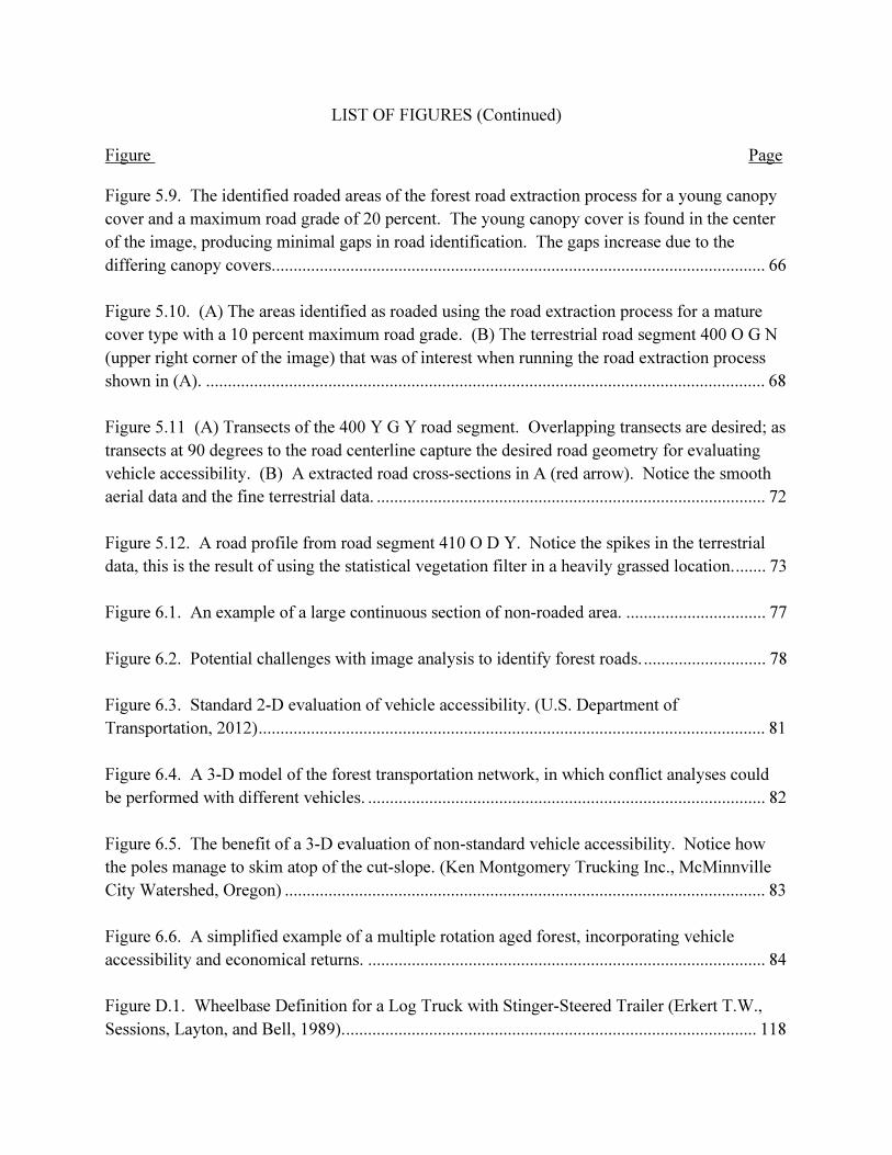
Figure 3.3. Hand digitized road centerline using a one meter DEM (White et al., 2010).
Craven et al. (2011) compared several methods of determining road centerline locations using
LiDAR. Four randomly assigned road segments of 256 meters in length were assigned in four
different forest cover types, 16 different road segments in total. Each road segment was
surveyed using a total station and two GPS established control points. Cross sections were taken
at a maximum spacing of 7.62 meters along each road segment, capturing centerline, edge of the
rocked portion of the road, geometric edge of road, ditch flow line, top of cut, and fill slope. The
surveyed road segments were compared to two different methods of determining road centerline
from the LiDAR data.
The first method explored by Craven et al. (2011) digitized the road centerline from visual
inspection of an intensity image and a visual inspection of the raw ground classified LiDAR

18
point cloud similar to the process of White et al. (2010). The intensity image was concluded to
produce the best results in approximating the field centerline. The second method used a
MATLAB script to automatically detect a road centerline and extract it using an initial guess of
the centerline location and adjusted the centerline location based on road width and slope. The
intensity image digitization performed better than the point cloud digitization in all four different
cover types compared to the field data. On average, the intensity image digitization had an
average horizontal difference of 0.89 m compared to the field-surveyed centerline. The point
cloud digitization had an average horizontal difference of 1.72 m compared to the field-surveyed
centerline. The extracted centerline from the intensity based extraction resulted in an average
error of 1.08 m difference compared to the field-surveyed centerline. The method that had the
lowest variation in extracting the centerlines was the intensity based extraction, 0.46 m standard
deviation, compared to the intensity based, 0.83m standard deviation, and the point cloud
digitization, 1.15m standard deviation (Craven et al., 2011).
Horizontal curves were measured using the three-point method, which has been known to have
errors up to 5% (Carlson et al., 2005). Craven et al. (2011) only reported on the comparison of
horizontal curves using the intensity based digitization and the field-surveyed data. The absolute
average difference of the curve radius was 3.17 m over all canopy types. The standard deviation
of these measurements indicated a large variability, 2.13 m of absolute difference in radius. The
vertical accuracy of the DEM was determined to have a root mean square error (RMSE) of 0.28
meters. The average difference in slope measurements from the intensity digitized centerline
compared to the field identified slopes was 0.57%.

19
3.1 Discussion
As discussed, these forest road identification processes use slope based methods to identify forest
roads however, none, use two attributes of LiDAR that are beneficial in identifying objects;
return intensity values, and return point densities. Developing an algorithm in which identifies
forest roads throughout an aerial LiDAR data set could prove useful in 3-D conflict analysis in
regard to vehicle accessibility. This algorithm would process aerial LiDAR data, filtering out
non-roaded areas, leaving behind only forest road areas. The process would differ from previous
work by using intensity values and point densities to identify forest roads; whereas pervious
work has focused on identifying forest roads by slope breaks and manual identification methods.
3.2 - Literature Cited
Carlson, P. J., Burris, M., Black, K., and Rose, E. R. (2005). Comparision of Radius-Estimating
Techniques for Horizontal Curves. Transportation Research Record: Journal of the
Transportation Research Board, 76-83.
Craven, M., Wing, M., Session, J., and Wimer, J. (2011). Assessment of Airborne Light
Detection and Ranging (LiDAR) for use in Common Forest Engineering Geomatic
Applications. M.S. Thesis, Oregon State Universtiy, College of Forestry, Corvallis.
Retrieved from Oregon State University: http://hdl.handle.net/1957/21803
Evans, J. S., and Hudak, T. (2007). A multiscale curvature algorithm for classifying discrete
return LiDAR in Forested Environments. IEEE Transactions on Geoscience and Remote
Sensing, 45, 1029-1038.

20
Rieger, W., Kerschner, M., Reiter, T., and Rottensteiner, F. (1999). Roads and Buildings from
Laser Scanner Data in a Forest Enterprise. International Archives of Photogrammetry and
Remote Sensing Workshop, 32, pp. 185-191. LaJolla, California.
White, R. A., Dietterick, B. C., Mastin, T., and Strohman, R. (2010). Forest Roads Mapped
Using LiDAR in Steep Forested Terrain. Remote Sensing, 2(4), 1120-1141.

Chapter 4 - Registration of Terrestrial LiDAR Data Sets
4.1 - Background
4.1.1 - Study Area
Two road systems were sampled within the McDonald and the Paul M. Dunn Forests
(McDonald-Dunn Research Forest). A map of the study area and road sample locations can be
found in the Appendix. The McDonald-Dunn Research Forest is located seven miles north of the
Oregon State University (OSU) campus. The forest consists of approximately 4,552 hectares of
forested land along the western edge of the Willamette Valley and the eastern foothills of the
Coast Range. With four distinct management themes, the forest is extensively used for
university teaching, demonstration and research (Fletcher, et al., 2005).
4.1.2 - Datasets
To assess the potential of LiDAR, nine terrestrial LiDAR samples were collected throughout the
McDonald-Dunn Forest, Corvallis, Oregon. A sample is defined as several (5-8) terrestrial
LiDAR scans geo-referenced together as a single point cloud. The goal of this research is to
compare road geometry characteristics between aerial and terrestrial LiDAR databases. An
airborne LiDAR survey of the McDonald Forest was completed in 2008 by Watershed Sciences,
Inc. The terrestrial LiDAR data sets were collected in 2012 by Oregon State University. This
provided a four year time period between the two data sets. Acknowledging that the

22
transportation network is always changing, areas of high activity since 2008 were be eliminated
from the comparison. The comparison will be limited to areas of no activity (harvesting, heavy
traffic, and road maintenance) since 2008. Harvesting, heavy traffic, and road maintenance over
the past four years would basis the validation procedure and skew the results.
The areas of no activity throughout the McDonald-Dunn Forest were determined through
interviews of the College Research staff and from activity databases. From these sources, six
road systems were identified as possible candidates for the comparison. These road systems
were categorized by cover type and road surface categories. These categories were used to
identify the best possible conditions for the comparison and the worst possible conditions for the
comparison. From these six road systems, three were identified to be used in the analysis. The
road segments that were chosen were identified for the best and worst potential of road geometry
extraction, allowing for the focus on the best and worst case scenarios.
4.1.3 - Naming Convention
A consistent naming convention was used to minimize errors throughout the analysis. The
naming convention that was used was based on the administrative road number, cover type, road
surface, road vegetation, and any notes. The first portion of the road sample name is the
McDonald-Dunn Research Forest administrative road number. The second portion of the sample
name is the cover type category. Three cover types were identified; (1) Mature (M), (2) Old
even aged (O), (3) Young even aged (Y), (4) Clear Cut or Meadow (C). The third portion of the
sample name was determined from the road surface type. Only two surface types were identified

23
(1) gravel (G) and (2) dirt (D). The next portion of the sample name was determined by the
presence of vegetation in the road surface; (Y) for if there was vegetation present and (N) if there
was no vegetation present. The last portion of the name was determined by unique
characteristics of the road. These notes were spelled out in the sample name. For example,
sample that was located on the 260 road, with an old cover type, a gravel road surface, with
vegetation and no special characteristics would be named 260_O_G_Y. Table 4.1 shows all of
the road samples with implemented naming convention.
Table 4.1. Road sample naming convention.
Road
No.
Cover
Type
Road
Surface Vegetation Notes Sample Name
260 O G Y 260_O_G_Y
410 O D Y 410_O_D_Y
240 C D Y 240_C_D_Y
420 O G N 420_O_G_N
400 O G N 400_O_G_N
400 M G N 400_M_G_N
400 Y G Y 400_Y_G_Y
260 O G Y 2 260_O_G_Y_2
400 C G Y 400_C_G_Y
4.2 - Methodology
4.2.1 - Data Collection
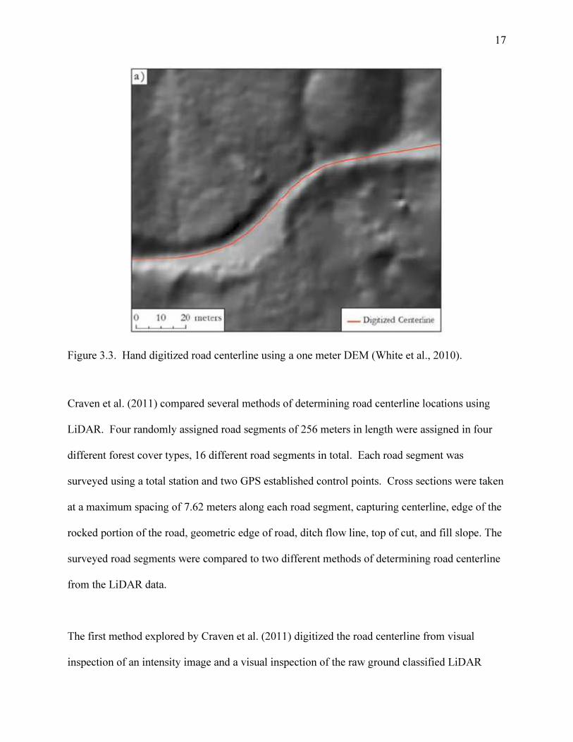
The road segments were collected using a FARO FOCUS3D laser scanner (Figure 4.1) and six
sphere targets (Figure 4.2) throughout June and August 2012. The FARO FOCUS3D was set at a
resolution of 0.006 degrees and a 15 degree (above the horizontal axis of the scanner) cut off.
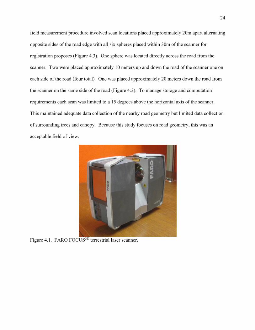
The sphere targets were 152.4 mm in diameter and made of a durable matte-white polyester. The
24
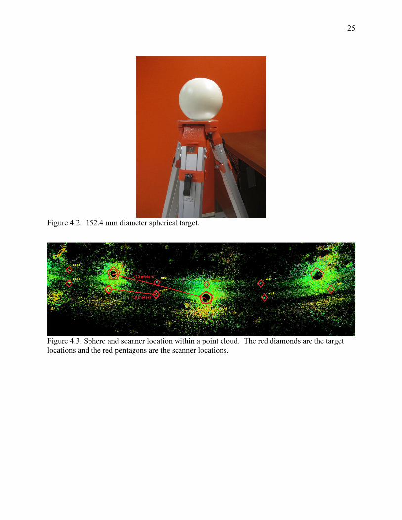
field measurement procedure involved scan locations placed approximately 20m apart alternating
opposite sides of the road edge with all six spheres placed within 30m of the scanner for
registration proposes (Figure 4.3). One sphere was located directly across the road from the
scanner. Two were placed approximately 10 meters up and down the road of the scanner one on
each side of the road (four total). One was placed approximately 20 meters down the road from
the scanner on the same side of the road (Figure 4.3). To manage storage and computation
requirements each scan was limited to a 15 degrees above the horizontal axis of the scanner.
This maintained adequate data collection of the nearby road geometry but limited data collection
of surrounding trees and canopy. Because this study focuses on road geometry, this was an
acceptable field of view.
Figure 4.1. FARO FOCUS3D terrestrial laser scanner.
25
Figure 4.2. 152.4 mm diameter spherical target.
Figure 4.3. Sphere and scanner location within a point cloud. The red diamonds are the target
locations and the red pentagons are the scanner locations.

26
Figure 4.4. Sphere and scanner location on a road segment
To be able to perform a ridged body transformation to the UTM coordinate system, NAD83
(CORS96) Epoch 2002.00, three control points were used within each sample, one at the
beginning, middle, and end scan locations. The control points were PK nails with color coded
flagging attached (Figure 4.4). A spherical target was centered on top of the PK nail and leveled
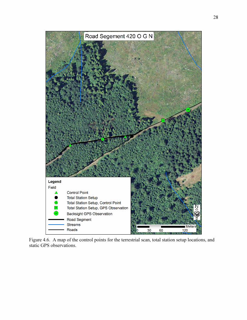
using a bipod and a five second level bubble (Figure 4.5). Depending on the canopy cover, the
control points were either surveyed using a total station which was tied to two static GPS
observations (one to start the traverse from and one to set the backsight) or the control points
were directly surveyed using a static GPS observation (Figure 4.6). Topcon HiperLite+ GPS
Units (Figure 4.7Figure 4.7) were used to establish control points for the total station surveys and
were used to directly survey control points in clearcuts and young canopies. The GPS

27
observations were static GPS observations, observing for at least eight hours, sometimes longer
depending on sky plot visibility. The Online Positioning User Service (OPUS) was used to post
process all GPS observations (National Geodetic Survey, 2012).
Figure 4.5. A close up image of the scanner and target setup at a middle control point.
28
Figure 4.6. A map of the control points for the terrestrial scan, total station setup locations, and
static GPS observations.

29
Figure 4.7. Topcon HiperLite+ GPS Unit.
A static GPS observation is an observation of a single point for at least two hours (National
Geodetic Survey, 2012). To improve the accuracy of the static observation, it is recommended to
have longer observation times and to use the precise ephemeris in post processing. As the
observation time increases the ability to reduce ionospheric refraction, tropospheric refraction,
multipath, and receiver noise errors are reduced. Under ideal conditions and an observation
duration of eight hours, the horizontal root mean square (RMS) value stabilizes around 0.25 cm
and the vertical RMS value is approximately 1.25 cm (National Geodetic Survey, 2012). To
process the static GPS observations OPUS was used. OPUS is a web service, which allows

30
access to high-accuracy National Spatial Reference System (NSRS) coordinates. OPUS uses the
PAGES software program to compute position coordinates based on continuously operating
reference stations (CORS) (National Geodetic Survey, 2012). The software averages the
coordinates from at least three independent CORS by using double differenced carrier-phased
measurements (National Geodetic Survey, 2012). The results of the GPS observations are shown
in Table 4.3.
With coordinate for the control points established, total station traverses were conducted using a
Nikon Nivo 5.C total station and two circular prisms. The Nikon Nivo 5.C total station had a 5
second angle accuracy, and a 3 mm plus 2 parts per million distance accuracy. Bipods with a 5
second bubble level were used to level the prism rods while total station shots were being taken.
All traverses were closed to at least Third Order Class II specifications, which have a position
closure error of 1:5,000 (Federal Geodetic Control Committee, 1984). The tolerances of each
survey can be found in Table 4.2. The traverses were rotated, shifted, and scaled based on the
starting GPS control point and the azimuth GPS control point (Figure 4.6).
Table 4.2. Tolerances of surveys.
Traverse Road Segment(s) Closure Error
1 400O G N, 410 O D Y 6,167
2 420 O G N 9,880
3 400 M G N 10,917
4 260 O G Y, 260 O G Y 5,714

31
Table 4.3. Static GPS observation results, all measurements are in meters.
Peak to Peak Error UTM
Point Date
Orbit
Type RMS
Obs.
Used
Amb.
Fixed X Y Z Y X Z
240_C_D_Y
Start Pt 7/10/2012 Precise 0.016 98% 90% 0.005 0.018 0.002 4949597.644 476713.868 262.092
240_C_D_Y
Mid Pt 7/24/2012 Precise 0.016 97% 88% 0.012 0.280 0.013 4949546.280 476683.380 265.673
240_C_D_Y
End Pt 7/24/2012 Precise 0.018 78% 84% 0.012 0.002 0.018 4949482.433 476706.677 265.468
400_C_G_Y
Start Pt 7/31/2012 Precise 0.019 88% 88% 0.004 0.006 0.009 4947441.254 477804.202 178.075
400_Y_G_Y
End Pt 8/1/2012 Precise 0.016 93% 89% 0.025 0.033 0.052 4947414.407 476683.041 302.364
400_Y_G_Y
Mid Pt 8/1/2012 Precise 0.016 91% 93% 0.006 0.022 0.012 4947405.962 476600.904 290.427
400_Y_G_Y
Start Pt 8/1/2012 Precise 0.018 87% 88% 0.007 0.003 0.011 4947354.575 476616.656 280.346
400_C_G_Y
Mid Pt 8/1/2012 Precise 0.013 94% 96% 0.010 0.004 0.013 4947420.941 477752.711 178.481
400_C_G_Y
End Pt 8/2/2012 Precise 0.021 70% 81% 0.035 0.030 0.047 4947395.394 477673.740 180.968
200_C_G_N_2
Start Pt 8/3/2012 Precise 0.016 80% 90% 0.012 0.026 0.056 4949464.005 476807.485 264.755
200_C_G_N_2
End Pt 8/3/2012 Precise 0.016 97% 86% 0.016 0.023 0.020 4949592.113 476844.464 245.042
200_C_G_N_2
Mid Pt 8/7/2012 Precise 0.015 95% 82% 0.022 0.021 0.029 4949519.210 476811.936 257.779

32
4.2.2 - Registration
The next two sections will explain the two registration processes used to determine an acceptable
registration error. The Register-then-Transform process describes registering scans together and
then performing a rigid body transformation. The Register-and-Transform process describes
registering scans together at the same time of the rigid body transformation.
4.2.2.1 - Register-then-Transform
Register-then-Transform, is relatively straightforward two-step process. After the scans were
imported into a software program, the spherical targets were automatically detected in each scan
and the scans were registered together using a least squares adjustment process. The least
squares adjustment process is described in Equation 1. Through the target detection process, the
software named common targets to its best estimate. With the targets named, the software then
registered the scans together, using only the targets and the inclination sensor readings from the
scanner. After the registration process, the user is responsible for ensuring the scans were
properly registered and the errors between targets were appropriate. Once the scans were
registered they were shifted and rotated to the control points as a unit.
��� � = ∑ �������� + ∑ �����
��� + ∑ �������� (1)
Where
���= the difference between the control value and the transformed value for point i, in x
���= the difference between the control value and the transformed value for point i, in y

33
���= the difference between the control value and the transformed value for point i, in z
�= the sum of the residuals
4.2.2.2 - Register-and-Transform
Register-and-Transform was significantly more involved than Register-then-Transform. To be
able to register the individual scans together using the second registration process, each
individual scan file needed to be imported into Cyclone, creating a scan world for each scan
location. Within each scan world, all of the sphere targets were isolated and modeled. The
modeled spheres were used to create a vertex for use in the registration process. Each vertex was
named accordingly (Figure 4.8).
Figure 4.8. Naming convention used during the second registration process.
With the vertices named, the control coordinates were imported into Cyclone as a scan world and
used in the registration process. The first registration process used was target-only registration,

34
to establish a preliminary registration. The preliminary registration was used to provide a close
registration to aid in the iterative closest point (cloud-to-cloud) registration process. The cloud-
to-cloud constraints that were added were (a) the scan positions that were next to each other and
(b) scans that were spaced one scan position between each other. For example, scan position 1
and scan position 2 had a cloud-to-cloud constraint added, and scan position 1 and scan position
3 had a cloud-to-cloud constraint added. This produced 13 cloud-to-cloud constraints. With all
of the target and the cloud-to-cloud constraints added, the scans were registered together. A few
of the cloud-to-cloud constraints produced under-constrained errors (even after settings were
adjusted) and were not used in the registration process. This error seemed to occur more
frequently on road samples in clearcuts where few distinct objects were identifiable.
4.3 - Results
4.3.1 - Data Collection
The average number of points per scan was 66.5 million; totaling to an average number of points
per road sample of 531.9 million (Table 4.4). The road samples that were located within
clearcuts had the lowest points per scan due to the limited height of the vegetation. Samples that
were located within mature, old even-aged, or young even-aged stands provided larger number
of points per scan, due to the increase height of the surrounding vegetation.

35
Table 4.4. The number of points per scan location and road sample.
Segment Name Number of Points
(millions) Num. of Scans
Average pts/Scan
(millions)
260_O_G_Y 554.5 8 69.3
410_O_D_Y 506.1 8 63.3
240_C_D_Y 432.6 8 54.1
420_O_G_N 561.8 8 70.2
400_O_G_N 563.2 8 70.4
400_M_G_N 569.4 8 71.2
400_Y_G_Y 528.5 8 66.1
260_O_G_Y_2 553.7 8 69.2
400_C_G_Y 503.5 8 62.9
Average 531.9 8 66.5
4.3.2 - Registration
4.3.2.1 - Register-then-Transform
Once all of the scans were registered together into a single coordinate system, the road segment
was then imported into Cyclone to for geo-referencing. The first step was to model the control
point spheres. Within each sample, only the three spherical targets that were over the control
points were modeled. The average modeled spherical target was 156.4 mm in diameter with a
standard deviation of 6.2 mm. The average number of points used to model a sphere was 17,902
points with a standard deviation of 7,160 points (Table 4.5).

36
Table 4.5. Fit statistics for the control spherical targets for the Register-then-Transform process.
Segment Name
Average (m)
Diameter STD No.
PTS STD
Error
Mean
Error
STD
ABS
Error
Mean
Max.
ABS
Error
260_O_G_Y 0.1562 0.0024 16,679 4,489 0.0000 0.0030 0.0021 0.0170
410_O_D_Y 0.1579 0.0042 27,401 12,635 0.0000 0.0023 0.0011 0.0246
240_C_D_Y 0.1532 0.0018 15,364 2,002 0.0000 0.0040 0.0021 0.0359
420_O_G_N 0.1548 0.0038 16,528 5,679 0.0000 0.0025 0.0012 0.0256
400_O_G_N 0.1554 0.0056 12,855 5,502 0.0000 0.0036 0.0018 0.0291
400_M_G_N 0.1571 0.0041 18,138 2,370 0.0000 0.0049 0.0031 0.0227
400_Y_G_Y 0.1590 0.0217 13,171 3,996 0.0000 0.0054 0.0043 0.0277
260_O_G_Y_2 0.1579 0.004 17,738 6,147 0.0000 0.0032 0.0017 0.0249
400_C_G_Y 0.1574 0.0055 21,112 12,273 0.0000 0.0042 0.0023 0.0260
Average 0.1564 0.0062 17,902 7,160 0.0000 0.0034 0.0021 0.0237
Register-then-Transform, produced unexpected results. Once the registered scans were
translated and rotated to the control points using a least squares adjustment, the average errors
were 17.1 cm for the Start control point, 5.0 cm for the Middle control point, and 17.2 cm for the
End control point (Table 4.6). These errors were larger than expected; the expected error was
approximately 2 cm for each control point. The target errors could be attributed to the fact that
the entire registered sample was rotated and translated after the scans were individually
registered together; not at the same time as done in Register-and-Transform. This result is
similar to what Olsen et al. (2011) found when geo-referencing costal sea cliff scans.
However, Register-then-Transform produced reasonable registration errors using only the targets
(Table 4.6). The average target error was 1.4 cm with a standard deviation of 0.5 cm. The
average maximum error between targets was 2.4 cm. From just focusing on the target
registration errors, it seems that Register-then-Transform, produced reasonable results; however
translating to real world coordinates is still a struggle using this process.

37
Table 4.6. Errors using Register-then-Transform. (MF- manual fit, no errors were computed)
Segment Name
Register-then-Transform (m)
Start Point Middle
Point
End
Point
Mean
target
errors
Max STD
260_O_G_Y 0.1119 0.0127 0.1230 0.0138 0.0210 0.0011
410_O_D_Y 0.1468 0.0392 0.1675 0.0124 0.0263 0.0059
240_C_D_Y 0.1618 0.0222 0.1626 0.0136 0.0226 0.0050
420_O_G_N 0.1672 0.0668 0.1623 0.0141 0.0252 0.0058
400_O_G_N 0.1732 0.0411 0.1909 0.0144 0.0238 0.0061
400_M_G_N 0.1735 0.0233 0.1958 0.0129 0.0255 0.0055
400_Y_G_Y 0.1847 0.1411 0.1080 MF MF MF
260_O_G_Y_2 0.1871 0.0580 0.1547 0.0149 0.0263 0.0062
400_C_G_Y 0.2073 0.0387 0.2364 0.0134 0.0235 0.0056
Average 0.1705 0.0501 0.1718 0.0135 0.0242 0.0052
4.3.2.2 - Register-and-Transform
The first process in Register-and-Transform process was to model all of the spherical targets. On
average 48 spherical targets were modeled within Cyclone within each sample. The average
molded spherical target was 152.6 mm in diameter with 3,571 points used to create the sphere
(Table 4.7). As the average reveals good results, standard deviation tells otherwise. The average
standard deviation of the diameter of the spheres was 4.7 mm and the average standard deviation
of the number of points used to model a sphere was 5,593 points.
38
Table 4.7. Fit statistics for the spherical targets for the Register-and-Transform process.
Segment
Name
Mean (m)
Diameter STD No.
PTS STD Error Mean
Error
STD
ABS
Error
Mean
Max.
ABS
Error
260_O_G_Y 0.1541 0.0050 3,506 5,349 0.0000 0.0018 0.0011 0.0162
410_O_D_Y 0.1525 0.0045 4,901 8,907 0.0000 0.0017 0.0011 0.0129
240_C_D_Y 0.1519 0.0038 3,265 4,827 0.0000 0.0020 0.0013 0.0167
420_O_G_N 0.1532 0.0045 3,261 4,568 0.0000 0.0020 0.0011 0.0195
400_O_G_N 0.1536 0.0043 2,741 3,700 0.0000 0.0019 0.0011 0.0200
400_M_G_N 0.1532 0.0050 3,805 5,949 0.0000 0.0016 0.0011 0.0137
400_Y_G_Y 0.1502 0.0053 3,116 4,818 0.0000 0.0020 0.0014 0.0157
260_O_G_Y_2 0.1520 0.0051 3,869 5,974 0.0000 0.0017 0.0012 0.0160
400_C_G_Y 0.1531 0.0048 3,677 6,249 0.0000 0.0018 0.0011 0.0173
Average 0.1526 0.0047 3,571 5,593 0.0000 0.0018 0.0012 0.0164
Register-and-Transform’s results produced significantly lower registration errors on the control
points (4.7). This is attributed to the ability of the software to register using control points,
targets, and cloud-to-cloud constraints together in a single registration process. This process
minimizes the total error of all constraints using a least squares adjustment while the first process
carries out two least squares adjustments; one for the scan worlds and one for the control points.
This difference in approach results in different solutions. The Register-and-Transform’s errors
on the control points were 5.0 cm for the Start control point, 3.2 cm for the Middle control point,
and 8.4cm for the End control point (Table 4.8).
The target only registration errors were on average 2.6 cm with a standard deviation of 1.2 cm.
The average maximum target error was 4.9 cm. The cloud-to-cloud average error was 2.8 cm
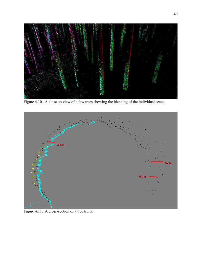
with a root mean squared (RMS) value of 1.9 cm. In addition to the errors produced by the
registration process, visual inspection was used. The scans were colored by scan position to

39
identify blending between point clouds (Figure 4.9 and Figure 4.10). Also a few cross-sections
were taken to estimate the differences between scan positions on a distinct object such as a tree
(Figure 4.11).
Table 4.8. Errors using Register-and-Transform.
Segment
Name
Register-and-Transform (m)
Start
Point
Middle
Point
End
Point
Mean
errors Max STD
Cloud-
to-
Cloud
(mean)
Cloud-
to-
Cloud
RMS
260_O_G_Y 0.0381 0.0076 0.0642 0.0286 0.0465 0.0131 0.0302 0.0112
410_O_D_Y 0.0492 0.0315 0.0959 0.0269 0.0449 0.0127 0.0289 0.0254
240_C_D_Y 0.0542 0.0490 0.0225 0.0255 0.0444 0.0106 0.0523 0.0190
420_O_G_N 0.0153 0.0378 0.0903 0.0264 0.0463 0.0131 0.0287 0.0119
400_O_G_N 0.0622 0.0131 0.1065 0.0340 0.0600 0.0146 0.0280 0.0106
400_M_G_N 0.0629 0.0107 0.1190 0.0318 0.0539 0.0128 0.0222 0.0118
400_Y_G_Y 0.0338 0.0639 0.1040 0.0274 0.0632 0.0147 0.0266 0.0168
260_O_G_Y_2 0.0709 0.0395 0.0620 0.0326 0.0694 0.0153 0.0317 0.0121
400_C_G_Y 0.0766 0.0185 0.1434 0.0354 0.0623 0.0149 0.0226 0.0151
Average 0.0497 0.0319 0.0844 0.0263 0.0490 0.0117 0.0282 0.0185
Figure 4.9. A road sample colored by scan position.
40
Figure 4.10. A close up view of a few trees showing the blending of the individual scans.
Figure 4.11. A cross-section of a tree trunk.

41
4.4 – Comparison
4.4.1 - Registration
The differences between the two registration processes were significant. The average difference
between the two methods is 11.0 cm on the Start control point, 1.2 cm on the Middle control
point, and 8.6 cm on the End control point (Table 4.9). This suggests that the ability to register
the scans together at the same time as registering the scan to real world coordinates is important.
Registering the scans together, then translating, and rotating the sample to the control
coordinates produces larger errors on the control points while minimizing the errors on the
targets, potentially resulting in a 10 cm increase in error on the control points. This result is
similar to what Olsen et al. (2011) found when geo-referencing costal sea cliff scans. When no
constraints were used when aligning scans together, there was poor agreement to RTK positions
obtained at scan origins (Olsen et al., 2011). Olsen’s findings were similar to the finding
discussed here; there were poor alignment to the control points when only target and/or point
cloud alignment techniques were used.
Table 4.9. Differences in registration errors of control points between Register-then-Transform
and Register-and-Transform.
Sample Name
Differences (m)
Start Point
Middle
Point End Point
Mean
errors Max STD
260_O_G_Y 0.0738 0.0051 0.0589 -0.0148 -0.0255 -0.0120
410_O_D_Y 0.0976 0.0076 0.0716 -0.0145 -0.0186 -0.0068
240_C_D_Y 0.1076 -0.0268 0.1401 -0.0119 -0.0218 -0.0056
420_O_G_N 0.1520 0.0290 0.0720 -0.0122 -0.0211 -0.0073
400_O_G_N 0.1111 0.0280 0.0844 -0.0196 -0.0362 -0.0085
400_M_G_N 0.1106 0.0125 0.0768 -0.0189 -0.0284 -0.0073
260_O_G_Y_2 0.1161 0.0185 0.0927 -0.0177 -0.0431 -0.0090
400_C_G_Y 0.1161 0.0185 0.0927 -0.0177 -0.0431 -0.0090
Average 0.1106 0.0116 0.0862 -0.0159 -0.0297 -0.0082

42
From this analysis, the Register-and-Transform process was used because the errors on the
control points were minimized while only a marginal increase in the target errors were observed.
In addition to the target errors, the visual inspection of the point clouds from the second
registration process seemed to produce a better overall fit compared to the first registration
process.
4.5 - Discussion
4.5.1 - Potential Problems
4.5.1.1 - Register-then-Transform
As mentioned previously, the ability to translate and rotate the scans to the control coordinates
simultaneous with the registration process greatly reduces the registration errors on the control
points. This is one potential shortcoming of the Register-then-Transform process. As seen in
Table 4.5 and 4.6, when only concerned with minimizing errors between scan locations the two
processes produce similar results, producing error propagation from the middle scan position
outward. This is because the registration process is concerned with minimizing the local fit
between the scans and small adjustments in rotation reduces errors in the targets but causes
larger global errors on the ends of the scans. In other words, this process produces reasonable
local results, but distorts the data from true geometric positioning accuracy. Another potential
shortcoming of the Register-then-Transform process is that stray points were filtered
automatically which may reduce the number of returns on the targets. The reduction in points on

43
a target could mean that the target is not able to be detected or accurately modeled by the
software. This process tended to occur when the spheres were placed >25 m from the scanner.
4.5.1.2 - Register-and-Transform
Some potential problems include over saturation and target shifting during the data collection
process (Figure 4.12) (Vosselman and Maas, 2010). The Register-then-Transform process might
correct for these two errors in the registration process. The Register-and-Transform process on
the other hand, did not have an inherent correction for these errors. Over saturation occurs when
the scanner is orthogonal to the target and the target is reflective (Vosselman and Maas, 2010).
This creates (in this case) a cone of returns that are closer to the scanner than the object is in
reality. Another possible error that was evident when visually inspecting the targets is that the
spherical target is shifted farther back from the scanner than the pole it is sitting on (Figure 4.13).
From a coarse inspection, it looks as though the target shift is approximately 5 cm away from the
scanner. A possible correction for this error is to determine the error based on the distance from
the scanner and shift all of vertices based on this error function. The target shift has previously
been identified with these reflective spheres (Russo, 2011). However, the target shift they
detected was approximately 2 cm, not the 5cm encountered. This target shift affected the overall
quality of alignment of the spheres after the registration process (Figure 4.13). If the target
points from individual scans positions were used to model a sphere the diameter of the modeled
sphere would be close (145-160 mm) to the actual diameter of the sphere (153 mm). However,
when the targets points from all scan positions were combined to model a single sphere, the
modeled diameter was approximately 133 mm, a significant difference in diameter of 20 mm.

44
The target shift and the smaller molded diameter spheres were the main reasons for the
registration errors between the scans and the control points.
Figure 4.12. Saturation (cone of points) and target shift away from scanner (center of sphere vs
center of pole).

45
Figure 4.13. Misalignment of sphere targets in registration process
4.6 - Conclusion
From our analysis we concluded, from the field data collection process used, the Register-and-
Transform process is more appropriate in minimizing and distributing errors throughout the
entire sample. The average errors produced by the Register-and-Transform process were 2.6 cm
on the targets, (1.2 cm standard deviation and 4.9 cm maximum) and 2.8 cm when combined
with a cloud-to-cloud registration (1.9 cm RMS). The average errors on the control points were
5.0 cm for the Start control point, 3.2 cm for the Middle control point, and 8.4 cm for the End
control point. These average errors on the control points still seem high but are a significant
reduction compared to the first registration process. However, this error magnitude is still

46
acceptable for measuring road geometry as driver error is more prevalent issue when determining
the accessibility of non-standard vehicles on a forest road than a measurement error of 8.5cm.
4.7 - Literature Cited
Federal Geodetic Control Committee. (1984). Standards and Specifications for Geodetic Control
Networks. Rockville.
Fletcher, R., Johnson, B., Blanchard, G., Hayes, J., Johnson, N., Johnson, D., Lysne, D., Murphy,
G., Newton, M.; Sessions, J. 2005. McDonald-Dunn Forest Plan. Last Accessed May 5,
2012, from http://www.cof.orst.edu/cf/forests/mcdonald/plan/files/mcdunn_plan.pdf
National Geodetic Survey. (2012, August 22). OPUS: Online Positioning User Service.
Retrieved from About OPUS: http://www.ngs.noaa.gov/OPUS/about.jsp#accuracy
Olsen, M., Johnstone, E., Kuester, F., Driscoll, N., Ashord, S. (2011, February). New
Automated Point-Cloud Alignment for Ground-Based Light Detection and Ranging Data
of Long Costal Sections. Journal of Surveying Engineering.
Russo, J. (2011, May 1). "Wow, that's weird. We've never encountered that...". Retrieved
December 5, 2012, from LiDAR News: http://www.lidarnews.com/content/view/8347/
Vosselman, G., and Maas, H.-G. (Eds.). (2010) Airborne and Terrestrial Laser Scanning.
Scotland, UK: Whittle Publishing

Chapter 5 - Forest Road Geometry Extraction and Comparison
Storm Beck, John Sessions, Michael Olsen, Michael Wing
5.1 - Abstract
The ability to identify the forest transportation network from LiDAR data could prove useful in
assessing vehicles accessibility throughout the forest transportation network. While prior work
has been able to detect centerlines, few studies have looked at identifying forest roads from
intensity values and density of returns, which could yield improved results. This study
investigates the identification of the forest transportation network using aerial LIDAR data. The
road extraction process uses two main attributes, which are intensity values and ground return
density. The road extraction process was developed using aerial LiDAR from McDonald-Dunn
Research Forest, Corvallis, Oregon. The road extraction process requires a text file with X, Y, Z,
coordinates and intensity values. The user must input also the canopy type of the file and the
maximum road grade encountered the area. To compare the results of the process nine road
segments were field surveyed using terrestrial LiDAR. The result of the road extraction process
identified 67% of the field surveyed roads based on length. Considering field surveyed gravel
roads alone, the success rate was 84% and 10% for native surface roads based on length. This
analysis was broadened to all roads within the canopy type of interest. It was determined that the
process identified 80% true positives, 34% false positives, 20% false negatives, and 38% true
negatives based on area. The average absolute value difference in the road width between the
two data sets were 1.1 m, while the cut/fill slope differences were minimal less than four percent
and the difference in road cross slope was two percent. These results were comparable with
48
other published studies comparing the differences between LiDAR measurements and field
measurements.
Keywords: LiDAR, Forest Transportation Network, Forest Road Extraction
5.2 - Introduction
The ability of vehicles to navigate the transportation network is based on both vehicle and
roadway characteristics. The roadway characteristics that influence a vehicle’s accessibility are
the road width, curve radius, curve widening, length of curve, cross-slope, and if overhang is
present the cutslope geometry and road edge obstructions. These characteristics are especially
important when evaluating non-standard vehicles, such as pole trailers and chip vans. These
non-standard vehicles allow for the transportation of high valued non-conventional products
(utility poles) or the production of low valued products (chips or hogfuel); providing
opportunities for the forest industry to increase economic value from forests. Currently, there are
two methods used when determining if a non-standard vehicle can access a certain portion of the
forest (1) field measurements and (2) visual inspection by the trucking contractor. Both of these
methods only evaluate portions of the transportation network. We investigate a method in which
forest roads and geometry can be identified and extracted from aerial LiDAR data to evaluate the
accessibility of non-standard vehicles in the forest transportation network.

49
5.3 - Background
Several studies have evaluated the horizontal and vertical accuracy of using aerial LiDAR data
for forest road measurements. For example, Rieger et al. (1999) approached mapping forest
roads to create break lines for more accurate digital terrain model (DTM) creation. White et al.
(2010) used a hill-shade approach to map forest roads in the Santa Cruz Mountains, California.
Craven et al. (2011) used different methods including hand digitization of the road centerline
from an intensity image and a point cloud image. In addition to the hand digitization, an
algorithm was created to identify the road centerline from an initial estimate of its location.
White et al. (2010) and Craven et al. (2011) produced similar results with centerline differences
less than 2 meters of the field surveyed centerlines.
While prior work has been able to detect centerlines, few studies have looked at identifying
forest roads from intensity values and density of returns, which could yield improved results.
Craven et al. (2011) used intensity images for the identification of forest roads but did not use
return densities to help in the identification process. This study examines the use of both
intensity values and return densities to identify and extract forest roads.

50
5.4 - Methods
5.4.1 - Extraction form Aerial LiDAR Data Sets
In this study, the process in which forest roads were extracted from LiDAR data sets were based
on two fundamental properties:
1) Intensity values on forest roads will be significantly different than those on the forest
floor as intensity values change with material properties (Figure 5.1) (Jenson, 2007)..
2) The density of ground returns on forest roads will be higher than those on the forest floor,
as canopy cover over a forest road is typically less than the canopy cover over the forest
floor (Jenson, 2007). This allows more returns to penetrate all the way through the
canopy and reflect off of the road surface.
Since different canopy conditions can occur along forest roads it is necessary to recognize
different forest canopy types and then to determine acceptable ranges of intensity values that
correspond to forest roads under different canopy types.
Three canopy types were chosen with the assumption the intensity values of ground returns
would vary enough between the three canopies to require identifying different intensity value
ranges for roads under these three canopy conditions (1) Clear cuts or Meadows, (2) Mature
Forests, and (3) Young Forests.
(1) Clear cuts or Meadows:
The forest road in a clear cut or a meadow is clearly visible with no obstructions from the
flight altitude

51
(2) Mature Forests:
A mature forest was defined as a forest that resembles older forest structure, with large
dominate trees with understory growth. The canopy cover over a forest road in these forests will
have areas with gaps visible from the flight altitude and areas that are completely closed in by
the surrounding trees and vegetation.
(3) Young Forests:
A young forest was classified as an even-aged forest between 15 and 35 years old. In
these forests the canopy cover over a road is an open corridor through a closed canopy. These
forests have not created a closed canopy structure over the roadway, but create a uniform layer
on both sides of the road between 15-45 feet tall in which return penetration is difficult and few
ground returns are obtained.

52
Figure 5.1. Intensity return map of a forested area in the McDonald Forest. The image is
colored by intensity values, dark indicating low intensity values and light indicating high
intensity values.
The intensity value ranges for the different canopy types were determined through
experimentation, however these ranges are specific to this data set. The ranges of acceptable
intensity values balance obtaining enough returns along the road and minimizing the number of
returns throughout the forest floor. The following steps will describe the preprocessing that is
required for each system.

53
Step (1):
Obtain LiDAR data files with only ground returns. The ground filtering method that was
used for our data was performed by Watershed Sciences and was assumed to be free of errors
(Watershed Sciences, 2008).
Step (2):
Obtain a starting range of values for each cover type. Subsets of points were selected
along segments of forest roads and the frequency of the intensity values was determined. The
intensity values that contained the majority of the returns were selected as the starting range
(Figure 5.2).
Step (3):
Determine if the range(s) of intensity values were too broad for each cover type. If this
was the case, the range(s) would then be adjusted until the returns selected were primarily on the
forest road producing a semi-continuous forest road selection and clumped or scattered non-
forest road selections (Figure 5.3).
The identified ranges for the different canopy types are listed in Table 5.1.

54
Figure 5.2. The second step in identifying an acceptable intensity value ranges for each cover
type. The red circles indicate the ranges in which a majority of the points fall within, this is
where a fine tuning of the ranges started.
Figure 5.3. The third step in the preprocessing steps of selecting appropriate intensity value
ranges for various canopy types.

55
Table 5.1. The determined intensity value ranges for identifying roaded areas.
Canopy Type Intensity Value Range
Clear Cut or Meadow 2 - 30
Young Forest 15 - 50
130 - 140
Mature Forest 40 - 80
140 - 170
The second principle of identifying forest roads from LiDAR data is determining point density
corresponding to a forest road (Figure 5.4). As seen in Figure 5.3, acceptable intensity values
were spread out across the entire area and not just constrained to forest roads. Several search
radii were used to locate areas of higher return densities and process these areas to distinguish
them from non-roaded areas. This process involved two facts, (1) forest roads will have a higher
ground return density than the surrounding areas and (2) forest roads are continuous and do not
have breaks. A filter was determined based on these two criteria to filter out isolated areas of
high return densities and to connect long enough segments of identified roaded areas together to
create a continuous forest transportation network (connection routine).

56
Figure 5.4. An illustration of the high ground return density along a forest road compared to the
surrounding forest floor.
The development of the connection routine is based on the maximum forest road slope that was
provided by the user and a predetermined distance between an isolated segment and the next
closest segment. In determining acceptable segments to join together, a process similar to a
recursive program solving forestry adjacency constraints was used. A grid was created of the
study area and each cell was identified if it contained at least one roaded return (Figure 5.5).
After identifying all of the cells that contained at least one roaded return, continuous segments of
roaded cells were identified. If the number of connected grids were less than 20, all returns
within those cells were removed from the roaded list. This process removed short isolated areas
from the solution (cells marked “O” in Figure 5.5). After removing short isolated areas from the
roaded list, the program adds cells back to the solution to connect isolated road segments. This
process is based on the assumption that forest roads are continuous and are not isolated. This

57
process used a shortest path connection routine with a constraint that no cell could be added to
the solution if the slope between the two cells is greater than the maximum road grade that the
user inputted. This maintained that the program not add a cell that created a slope greater than
the maximum road grade (cells with a “A” in Figure 5.5).
1 2 3 4 5 6 7 8 9 10 11 12 13 14 15 16 17 18 19 20
A O O
B O O
C X O O
D X O
E X
F X
G X X
H X A A A
I X A
J X A
K X X X X X X
L X X X
M O X X
N O X X
O X X
P O X X
Q O X X
R O X X
S O X X
T O X X
U O X X X
V O X
W O X
X O X
Y O X
Z O O
Figure 5.5. An example of the isolated and connection routines. Cells with an “O” will be
removed after the isolation routine and the cells with an “A” will be added after the connection
routine.

58
After this process was completed, the program created a Delaunay triangulation DTM of the
roaded list and then converts the Delaunay triangulation DTM to a grid. This conversion is done
by creating a list of points from the grid and determining the elevation for each point from the
Delaunay triangulation DTM. After the conversion, the grid is then saved as a floating point grid
file which could be imported into ArcGIS. The floating point grid file is used to compare the
differences between the aerial LIDAR dataset and the terrestrial LIDAR dataset. In addition to
the floating point grid file, the program exports out a text file of the roaded list in X, Y, Z, I
format. The work flow for the program is shown in Figure 5.6.

59
Figure 5.6 The workflow for the road extraction process. RL = roaded list, imin=minimum
acceptable intensity value, imax= maximum acceptable intensity value ADJ=adjacent, DTelv =
Delaunay Triangulation, GRIDRL= road list of the grid, csize=cell size, mgrade= maximum road
grade, mindist = minimum distance, {RL} = set of points in the road list, {N} = set of all ground
points, {GRID}= set of cells within the grid of the area, {ZADJ}=set of cells that are adjacent to
cell Z, {w}{p} = set of cells that connected to cell w, wpyc = the y coordinate of the center of the
cell connected to cell w, pz = the average elevation of cell p, -> = place into set

60
5.4.2 - Terrestrial LiDAR Data Collection
Six road systems throughout the McDonald-Dunn Forest were identified as possible candidates
for the comparison, excluding areas of activity between 2008 and 2012. These road systems
were walked and categorized by cover type and road surface. These categories were used to
identify the best possible conditions for the comparison and the worst possible conditions for the
comparison. Three road systems were identified to be used in the analysis. The road segments
that were chosen were identified for the best and worst potential of road geometry extraction.
The road segments were collected using a FARO FOCUS3D laser scanner and six sphere targets.
The FARO FOCUS3D was set at a resolution of 0.006 degrees. The sphere targets were 152.4
mm in diameter and made of a highly reflective and durable matte-white polyester. For each
sample, scans were completed approximately 20 m apart alternating opposite sides of the road
edge with all six spheres placed within 30 m of the scanner for registration proposes. Three
control points were set during the data collection, one at the start, middle, and end of the road
segment. A spherical target was centered on top of the control points and leveled using a bipod
and a five second level bubble.
Depending on the canopy cover, the control points were either surveyed using a total station
which was tied to two static GPS observations (one to start the traverse from and one to set the
backsight) or the control points were directly surveyed using static GPS observations with
Topcon HiperLite+ GPS unit. The GPS units observed for at least eight hours, sometimes longer

61
depending on sky plot visibility. The Online Positioning User Service (OPUS) was used to post
process all GPS observations.
The scan registration process used a least squares adjustment to register the scans together and to
perform a rigid body transformation of the scans to the control points. The average errors on the
control points were 5.0cm for the start control point, 3.2cm for the middle control point, and
8.4cm for the end control point.
5.4.3 - Statistically Filtering Terrestrial LiDAR Data Sets
After registering the terrestrial LiDAR data sets, vegetation was removed to be able to compare
the road prisms of the terrestrial and aerial data. A majority of the vegetation within the scans
were manually clipped out. To clean up the manual vegetation removal a statistical filter was
used to filter out the remaining vegetation. This statistical filter was based on the BIN ‘N’ GRID
process (Olsen, 2011). However, two enhancements were added (1) a comparison between the
user’s defined grid cell size and a one meter grid cell size and (2) a neighboring grid evaluation
comparison.
The comparison processes were developed to help remove non-ground returns on the edges of
the scan area or in areas where the amount of ground returns were minimal due to scan
placement and vegetation. On the edges of the scan area, the scanner has a difficult time
obtaining returns from the ground due to the scan angle and surrounding vegetation and
topography. This is evident when setting up the scanner on the cut slope side of the road (Figure

62
5.7). When the scanner is set up in this configuration it obtains few returns from the fill slope
due to the inability of the scanner to see the entire fill slope. In addition to not seeing the entire
fill slope from this angle, this process was developed to remove areas of the scan in which more
returns were obtained of vegetation than from the ground. The one meter grid size was chosen
based on a balance of maintaining original data integrity on the road and removing vegetation
along the edge of the road prism. To ensure that the comparison process did not coarsen the
data, the value of the one meter cell size had to be lower than any of the corresponding user
inputted cell size cells by three meters to overwrite the elevation value of the user input cell size
(Equation 1). This buffer was used to account for common road grades, cut, and fill slopes.
Figure 5.7. Typical forest road cross-section for a cut and fill section.

63
�� = �� � �� < ( �� + 3) (1)
Where
�� = elevation of user supplied cell size
�� = elevation of one meter cell size
The neighboring grid evaluation comparison was developed on the same principle as the first
comparison process; to remove non-ground returns from the data. This process determined the
average elevation and standard deviation of the neighboring cells without the center cell and
evaluated if the center cell was higher than the average elevation plus one standard deviation
(Equations 2-5). If the center cell was higher than this threshold then that cell elevation would
become the average elevation of the neighboring cells.
= ∑ ∑���
��
����
��� (2)
� = �∑ � ������
����
����� (3)
� = ∑ ���
����� (4)
� = � � ≥ + � (5)
Where
��= elevation of point i in neighboring cell j
�= mean elevation of center cell
�� = number of points in neighboring cell j
N = number of neighboring cells

64
n = number of points in the cell
nc = number of points in the center cell
= average elevation of the neighboring cells
� = standard deviation of the neighboring cells
This statistical filtering program enabled the user to select which of the seven statistical
processes they wanted to use (1) minimum (2) maximum (3) mean (4) standard deviation (5)
special (6) special with neighborhood (7) median or (8) all of the statistical processes. Once the
user selected the statistical process the user then entered the desired cell size. The program then
asks the user if they want to perform a quality control verification based on control points the
user created to reference the scans to real world coordinates. The program outputs four different
files (1) floating point grid file, (2) statistical file, (3) projection file, and (4) the quality control
verification difference file. Using these files, differences between the terrestrial and aerial road
geometry can be determined using ArcGIS.
5.4.4 - Road Geometry Extraction
With the two data sets filtered to only include road prism returns, transects were created through
the data to obtain cross-section views of the road segment to extract road prism variables using
the TopCAT program (Olsen, Young, and Ashford, 2012). This process required a centerline
and an ESRI grid file. A centerline was used to create transects along the centerline at a user
identified interval and length. These profiles were then reduced to points along the profile in

65
which X, Y, and Z coordinates could be determined. The profiles provided the ability to
determine the differences between the aerial and terrestrial data sets as seen in Figure 5.8.
Figure 5.8. The extracted transect from the road sample 400 Y G Y.
279.5
280.5
281.5
282.5
283.5
284.5
285.5
286.5
-10 -8 -6 -4 -2 0 2 4 6 8 10
Ele
va
tio
n (
m)
Profile Distance (m)
Terrestrial vs Aerial
Profile 25
400 Y G Y
Terrestrial
Aerial

66
5.5 - Results
5.5.1 - Road Extraction form Aerial LiDAR Data
Figure 5.9 provides an aerial photograph of a section of the LiDAR data overlaid with the GIS
forest road centerlines and the floating point grid file created from the road extraction process.
This figure shows the road extraction results from the road extraction routine for a young forest
canopy type and a 20 percent maximum road grade.
Figure 5.9. The identified roaded areas of the forest road extraction process for a young canopy
cover and a maximum road grade of 20 percent. The young canopy cover is found in the center
of the image, producing minimal gaps in road identification. The gaps increase due to the
differing canopy covers.

67
Once the road extraction process was run on all of the sample sites, the percentage of the
extracted road segments were calculated (Table 5.2). The extraction results can also be seen in
Appendix 1. The extraction process extracted 67 percent of the road prisms that were field
sampled with a terrestrial scanner. However, the process had a difficult time extracting native
surface roads, as evidenced by the 21 percent extraction on sample 410 O D Y and the zero
percent extraction on site 240 C D Y. If these two sites were removed; the road prism extraction
process would identify 84 percent of the road prisms that were field sampled.
Table 5.2. The road extraction results compared to the field measured road segments (sorted by
surface type than by covertype)
Segment
Name
Length of road
sample (m)
Length of road segment found by
the extraction process (m) Percentage
260 O G Y 2 181.1 169.5 94%
260 O G Y 240.7 109 45%
420 O G N 224.7 224.7 100%
400 O G N 205.1 96 47%
400 M G N 237 237 100%
400 Y G Y 308.3 308.3 100%
400 C G Y 209.7 209.7 100%
410 O D Y 184.7 38.1 21%
240 C D Y 149.7 0 0%
Average 67%
The major contributing factor of identifying non-roaded areas when using the road extraction
program was the extreme change of the canopy cover through the processed area and streams as
seen in Figures Figure 5.9 and Figure 5.10 (A). The road segment of interest (400 O G N) in this
area is shown in Figure 5.10 (B). It was a mature canopy type with the maximum road grade of

68
10 percent. The outcome of the road extraction was 47 percent but as seen by Figure 5.10 (A)
and Figure 5.10 (B), a majority of the area was identified as roaded. As seen in Figure 5.10 (B)
the southern half of the area is a farm field, which has higher point densities and different
intensity values than the mature canopy type. This difference in canopy covers in the study area
proved to be a weakness of the road extraction process.
Figure 5.10. (A) The areas identified as roaded using the road extraction process for a mature
cover type with a 10 percent maximum road grade. (B) The terrestrial road segment 400 O G N
(upper right corner of the image) that was of interest when running the road extraction process
shown in (A).
To further evaluate the effectiveness of the algorithm, false positives, false negatives, and true
negative were evaluated. These attributes were evaluated on an area basis, due to the difficulty
of determining lengths of non-roaded segments. To determine these attributes the areas of true
positive, false positive, false negative, and true negative values were determined (Table 5.3). As
identified in Table 5.3 the mean true positive was 81%, false positive 49%, false negative 19%

69
and true negative were 31%. However, as mentioned earlier, these values include canopy cover
types that were not necessarily of interest when running the road extraction process.
Table 5.3. Road extraction statistics for the entire study area. These statistics are biased by
including all cover types not just the cover type of interest.
False Positives False Negatives True Negatives True Positives
Clear Cut or Meadow Cover Type
Mean 20% 38% 64% 62%
STD 19% 18% 29% 18%
Min 7% 25% 44% 49%
Max 34% 51% 85% 75%
Mature Cover Type
Mean 63% 12% 20% 88%
STD 19% 5% 17% 5%
Min 40% 4% 3% 80%
Max 88% 20% 44% 96%
Young Cover Type
Mean 12% 27% 48% 73%
STD NA NA NA NA
Min 12% 27% 48% 73%
Max 12% 27% 48% 73%
Average
Mean 49% 19% 31% 81%
STD 28% 14% 26% 14%
Min 7% 4% 3% 49%
Max 88% 51% 85% 96%
To address this concern for road extraction of undesired areas, stratification was used to help
better identify the true values of the true positives, false positives, false negative, and true
negatives. Each area was stratified to the canopy type that was of interest during the road
extraction process. This resulted in more accurate results in identifying the results of the road
extraction process. rue negatives by seven percent.

70
Table 5.4 shows the results for the road extraction process when only considering areas of
interest. This resulted in a reduction of false positives by 15 percent, an increase of false
negatives by one percent, and an increase in true negatives by seven percent.
Table 5.4. Road extraction statistics for only cover types of interest.
False Positives False Negatives True Negatives True Positives
Clear Cut or Meadow Cover Type
Mean 32% 22% 49% 78%
STD 33% 27% 33% 27%
Min 9% 2% 26% 59%
Max 56% 41% 72% 98%
Mature Cover Type
Mean 38% 21% 38% 79%
STD 8% 13% 14% 13%
Min 27% 4% 16% 58%
Max 46% 42% 58% 96%
Young Cover Type
Mean 6% 12% 16% 88%
STD NA NA NA NA
Min 6% 12% 16% 88%
Max 6% 12% 16% 88%
Average
Mean 34% 20% 38% 80%
STD 16% 14% 18% 14%
Min 6% 2% 16% 58%
Max 56% 42% 72% 98%
The results of the road extraction process produced the following results: false positives 34%,
false negatives 20%, true negatives 38%, and true positives 80%. As seen by this analysis,
extreme differences in cover type throughout an area will have a large impact on the results of
the road extraction process mostly in false positives, as shown in Figure 5.10

71
5.5.2 - Road Geometry Comparison
The TopCAT profile extraction process provided X, Y, and Z coordinates of evenly spaced
points along the profile (Figure 5.11). Transects were spaced 5 meters apart and points within a
transect were spaced 0.5 meters apart. This spacing provided a high resolution of the road prism
compared to conventional road prism measurements, which usually only collects data points on
the road edges, centerline, top of the ditch, bottom of the ditch and the top of the cut slope and
the bottom of the fill slope, road transects are usually spaced between 7.62-15.24 meters apart,
providing a balance between accuracy of the road geometry and speed of the survey.
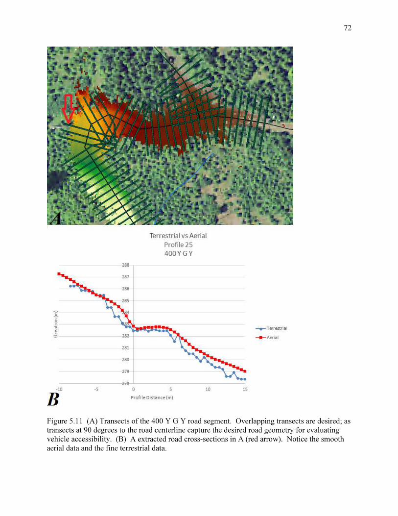
72
Figure 5.11 (A) Transects of the 400 Y G Y road segment. Overlapping transects are desired; as
transects at 90 degrees to the road centerline capture the desired road geometry for evaluating
vehicle accessibility. (B) A extracted road cross-sections in A (red arrow). Notice the smooth
aerial data and the fine terrestrial data.

73
With this data, road geometry variables were extracted from this data. The extracted variables
were the road width, cross-slope, and the cut or fill slope. One of the challenges when extracting
this data was that the road prism was not always easy to detect as in Figure 5.11. For example,
road segment 410 O D Y, (Figure 5.12) was extremely difficult to identify the road prism.
Figure 5.12. A road profile from road segment 410 O D Y. Notice the spikes in the terrestrial
data, this is the result of using the statistical vegetation filter in a heavily grassed location.
Even with the challenges of identifying some road prisms, the differences between the aerial and
terrestrial road geometry were consistent. The average absolute value difference between the
road width between the aerial and terrestrial data was 1.1m, the average absolute difference
136.9
137.1
137.3
137.5
137.7
137.9
138.1
-10 -8 -6 -4 -2 0 2 4 6 8 10
Ele
va
tio
n (
m)
Profile Distance (m)
Terrestrial vs Aerial
Profile 30
410 O D Y
Terrestrial
Aerial

74
between the cross slope and the left cut/fill slope was three percent, while the difference between
the right cut/fill slopes was four percent (Table 5.5). These results are on par with other studies
of the differences in aerial LiDAR road geometry and field measurements (Craven et al., 2011,
White et al., 2010).
Table 5.5. The summary table of the difference between the extracted road geometry variables.
All measurements are in meters.
Mean STD Max Min
Road Width 1.1 0.2 5.5 0.1
Cross Slope 2% 2% 12% 0%
Left cut/fill slope 3% 4% 70% 0%
Right cut/fill slope 4% 5% 56% 0%
5.6 - Conclusion
The road extraction process was successful in identifying 67 percent of the roads that were field
sampled. If native surface roads were removed from the analysis, the process successfully
identified 84 percent of the forest roads segments by length. This process proved to be generally
successful in identifying forest gravel roads but was unsuccessful in identifying forest native
surface roads. For roads that were within the cover type of interest, this process identified 80
percent of the roads. The road geometry comparison between the aerial and terrestrial data sets
agreed with other published results (Craven, et al., 2011 and White, et al., 2010). The average
difference in the road width between the two methods was 1.1m, while the cut/fill slope
differences were minimal less than four percent and the difference in road cross slope was two
percent.

75
The largest difference between the two methods was the resolution of data. As seen in Figure
5.11 (B) and Figure 5.12 the aerial road profile was not able to show the small changes in the
road surface, ditch width, or road edge as made evident in the terrestrial data. The aerial data
was not able to identify ruts in the running surface as seen in Figure 5.12. From this analysis it is
possible to identifying forest roads based on intensity values and point densities using aerial
LiDAR data. This will prove useful when trying to extract forest road geometry across the entire
forest transportation network to evaluate the accessibility of non-standard vehicles.
5.7 - Literature Cited
Craven, M., Wing, M., Sessions, J., and Wimer, J. (2011). Assessment of Airborne Light
Detection and Ranging (LiDAR) for use in Common Forest Engineering Geomatic
Applications. M.S. Thesis, Oregon State Universtiy, College of Forestry, Corvallis.
Retrieved from Oregon State University: http://hdl.handle.net/1957/21803
Jenson, J. R. (2007). Remote Sensing of the Environment: An Earth Resource Perspective. (J.
Howard, D. Kaveney, K. Schiaparelli, & E. Thomas, Eds.) Upper Saddle River, NJ:
Pearson Prentice Hall.
Olsen, M. (2011, May 29). Bin ‘n’ grid: A simple program for statistical filtering of point cloud
data. Retrieved from http://www.lidarnews.com/content/view/8444/208/
Olsen, M. J., Young, A. P., and Ashford, S. A. (2012). TopCAT- Topographical Compartmetn
Analysis Tool to Anlyze seacliff and beach change in GIS. Computers & Geosciences,
284-292.
Watershed Sciences. (2008). LiDAR Remote Sensing Data Collection: McDonald-Dunn
Research Forest. Corvallis, Oregon: Wastershed Sciences Inc

Chapter 6 - Conclusion and Future Research
The contributions of this thesis were identifying forest roads using intensity values and point
densities. It was theorized that gravel and native surface roads could be identified using LiDAR.
This hypothesis was tested by collecting a subsample of road geometries using terrestrial LiDAR
and comparing them to extracted road geometries from aerial LiDAR data sets. The field
collected data was collected in a manner focusing on the best and worst case road extraction
potential. This provided the opportunity to identify the limits of the technology rather than focus
on the average. The road extraction process identified 67 percent of the roads that were field
sampled by length. Separating native surface roads and gravel roads, the process identified 10
percent of the native surface roads and 84 percent of the gravel roads. In addition, to the
identification challenges on dirt roads, the ability to determine the road geometry on these roads
was a challenge using LiDAR. This was because on the dirt roads that were sampled, the road
geometry points were not well defined compared to the road geometry points of gravel roads.
This could be attributed to the functional use, maintenance, and vegetation growth on these
roads.
6.1 - Future Research Areas
The forest road extraction process proved to produce better results under consistent canopy types
compared to extreme changes in canopy cover. When used through areas with extreme changes
in canopy covers such as a farm field and a mature canopy cover, the process identified large
areas of non-roaded areas as roaded areas (Figure 6.1). A possible future adjustment to this

77
algorithm would be to implement a process in which large continuous areas were evaluated to
determine if they were too large to be a road. This process would remove large sections of non-
roaded areas from the solution, such as shown in Figure 6.1.
Figure 6.1. An example of a large continuous section of non-roaded area.
Another potential future research area would be to add an image analysis process to help further
identify roaded areas. This process would have to take into account the difficulty to “see” forest
roads from imagery due varying canopy cover, as shown in Figure 6.2. The combination of an

78
image analysis algorithm and the road extraction process based on intensity values and point
densities could greatly aid in forest road identification. To further aid in vehicle accessibility
throughout the forest transportation network a thinning algorithm could be used to reduce the
identified roaded areas to centerline locations. These centerline locations could then be used as
the vehicle paths throughout the network and using a 3-D model of the forest road network a
conflict analysis could be conducted. The implementation of these additional processes would
continue the effort of evaluating non-standard vehicle accessibility throughout the entire
transportation network.
Figure 6.2. Potential challenges with image analysis to identify forest roads.

79
6.2 - Quality Assessment
6.2.1 - Effect of Vehicle Type on Needed Data Quality
When assessing the accessibility of vehicles throughout the transportation network the road
geometry that is being used to assess the vehicles would need to be of appropriate in quality.
The required quality of the road geometry is dependent on vehicle type being assessed. This is
identified when comparing the various off-tracking methods. From the comparison of off-
tracking models in Appendix 4, the mean road width required for the standard log truck case was
3.82 meters with a standard deviation of 0.10 meters (Appendix D). The mean road width
required for the pole truck case was 6.37 meters with a standard deviation of 0.55 meters
(Appendix D). This illustrates that the six different methods will provide six different solutions
to a vehicles’ accessibility throughout the forest transportation network. It creates another
question to ask when trying to determine what quality of road geometry is needed to provide
accurate vehicle accessibility solutions.
6.2.2 - Comparison of LiDAR Results to Conventional Field Equipment
Putting the differences in the off-tracking equations aside, it could be assumed that the quality of
road geometry needed to determine vehicle accessibility throughout the forest transportation
network would need to be at least the same level of accuracy that is achieved when collecting
field measurements using conventional forest engineering equipment. This equipment typically
includes a clinometer, a hand compass, and a Spencer's tape. A clinometer can be read to the
80
nearest percent (Suunto, 2007). A hand compass can be read at two-degree intervals (Suunto,
1998). A Spencer's tape can be read to a 100th of a foot. Although this is the stated accuracy of
the equipment; being able to measure the road width down to a 100th of a foot is unrealistic, due
to the nature of a forest road. One would assume that a more realistic measurement accuracy of
road widths would be 0.18 to 0.3 meters and grade and cut-slope geometry would be within five
percent. The complexities of the cut-slope and a generalization that occurs during conventional
field data collection dictates this level of accuracy. If this accuracy level has been the standard in
the past, then from the sampled road segments and differences in road geometry, LiDAR has the
accuracy needed to determine vehicle accessibility throughout the forest transportation network.
6.3 - 3-D Vehicle Analysis
In addition to 2-D evaluation of the accessibility of specialized vehicles in the transportation
network (Figure 6.4), LiDAR can provide the ability to evaluate specialized vehicle accessibility
on a more complex 3-D scale (Figure 6.5). This 3-D evaluation of vehicle accessibility started in
the civil transportation field with the use of programs such as AutoTURN Pro 3D. AutoTURN
(Carrasco, 1992), that was designed for common urban vehicles and used primarily for urban
transportation design. Its development in the recent years, has included the effects of cross
slope for common urban vehicles on pavement and 3-D turn simulations (Gochngbok, 2012).
The use of a 3-D turn simulation model for evaluating the accessibility of specialized vehicles
throughout the transportation network would lead to identifying proper speed limits on road
segments by incorporating sight distances around curves and identifying pinch points in the
transportation network (Figure 6.5). A pinch point is a location within the transportation

81
network, where the location limits the accessibility of the vehicle; however before and after this
location the vehicle can freely traverse the transportation network. Possible pinch points include
sharp corners with not enough curve widening, steep adverse grades, and steep cut-slopes or
obstructions along the road way that confine overhang sweep.
Figure 6.3. Standard 2-D evaluation of vehicle accessibility. (U.S. Department of
Transportation, 2012)

82
Figure 6.4. A 3-D model of the forest transportation network, in which conflict analyses could
be performed with different vehicles.

83
Figure 6.5. The benefit of a 3-D evaluation of non-standard vehicle accessibility. Notice how
the poles manage to skim atop of the cut-slope. (Ken Montgomery Trucking Inc., McMinnville
City Watershed, Oregon)
6.4 - Potential Benefits
Identifying the pinch points, would lead to the economic analysis of determining the investment
cost of removing the pinch point and the economic benefit of hauling non-conventional products
from beyond the pinch point. In addition to the economic benefit of hauling non-conventional
products, the ability to have a forest ownership under different rotation ages based on market
demands and the accessibility of specialized vehicles provides an enhanced ability to manage for
forest health risks. Forest health risks include insects, disease, fire, and wind damage (Tappeiner
II, Maguire, and Harrington, 2007). A multiple rotation aged forest could provide a larger

84
diversification of the landowner’s investment and reduce the risk of insect, disease, fire, and
wind damage.
Figure 6.6. A simplified example of a multiple rotation aged forest, incorporating vehicle
accessibility and economical returns.
Instead of the common single rotation age forests, forests would be managed under multiple
rotation ages, contributing to economic, environmental, and societal benefits such as shown in
Figure 6.6. This management scheme incorporates vehicle and product accessibility and product
production potential throughout the forest, adding to forest value. This combination of varied
rotation ages has the potential to address economic concerns while reducing potential forest
health risks and also providing societal benefits. As more pressure is placed on the forest

85
industry to produce more lumber while reducing environmental impacts a more diversified forest
landscape such as discussed could be one method to meet these increasing pressures.
6.5 - Literature Cited
Carrasco, M. S. (1992, January). Computerized Vehicle-Turning Simulation- An Interactive
Gochngbok, M. (2012, January 10). AutoTurn Pro 3D. (S. Beck, Interviewer)
Suunto. "Optical Reading Clinometer." Suunto User's Guide PM-5. Valimotie: Suunto Oy,
October 2007. 15.
Suunto. "The Suunto MC-1 Compass." Instructions for use of Suunto MC-1 Mirror Compass.
Espoo: Suunto Oy, 1998. 5.
Tappeiner II, J. C., Maguire, D. A., & Harrington, T. B. (2007). Silviculture and Ecology of
Western U.S. Forests. Corvallis: Oregon State University Press.
U.S. Department of Transportation. (n.d.). Retrieved January 15, 2012, from Chapter VI: Road
Geometry: http://www.fhwa.dot.gov/policy/otps/truck/wusr/chap06.htm

86
Appendix A
Aerial Road Extraction Results

87

88

89

90
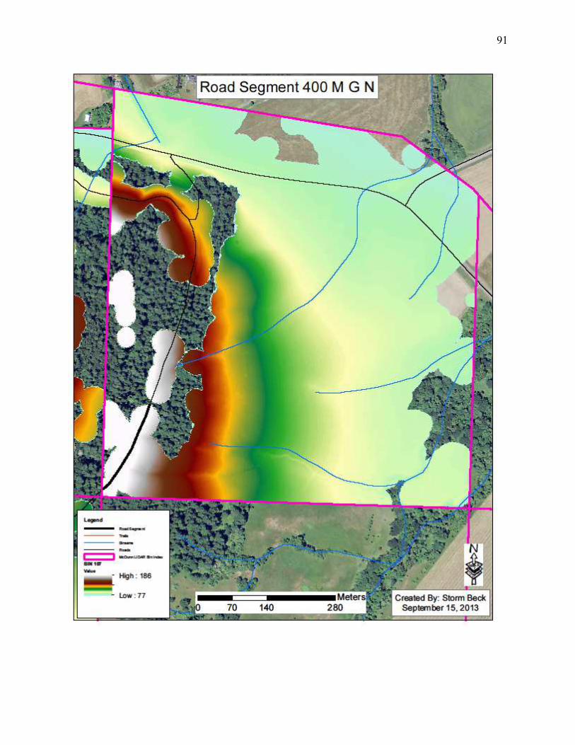
91
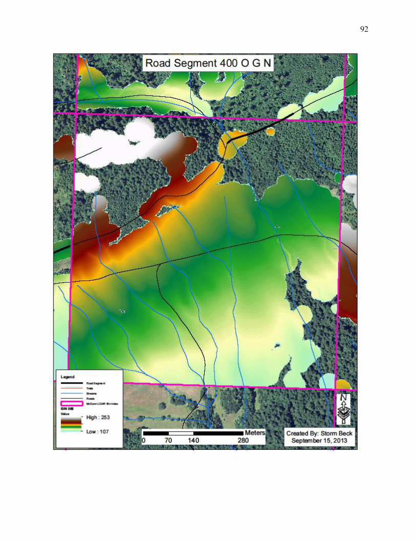
92

93

94
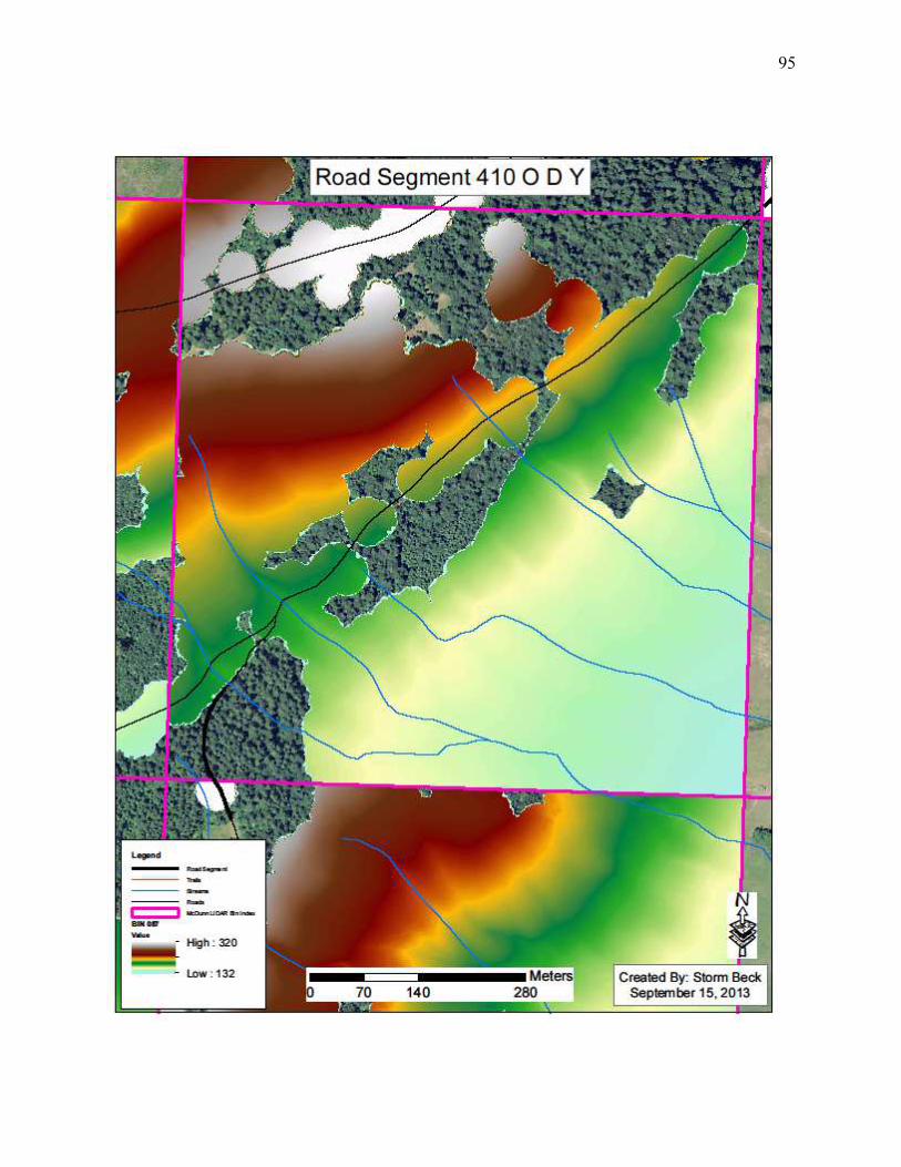
95

96

97
Appendix B
Terrestrial Road Segments

98
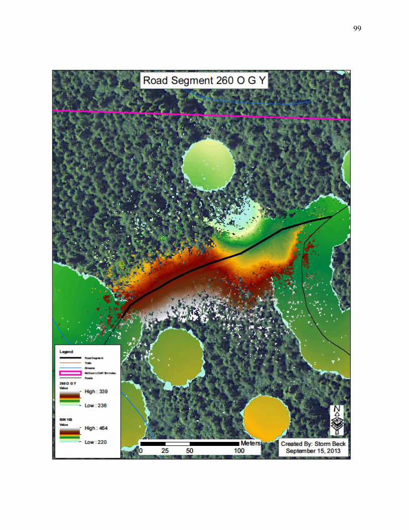
99

100

101

102
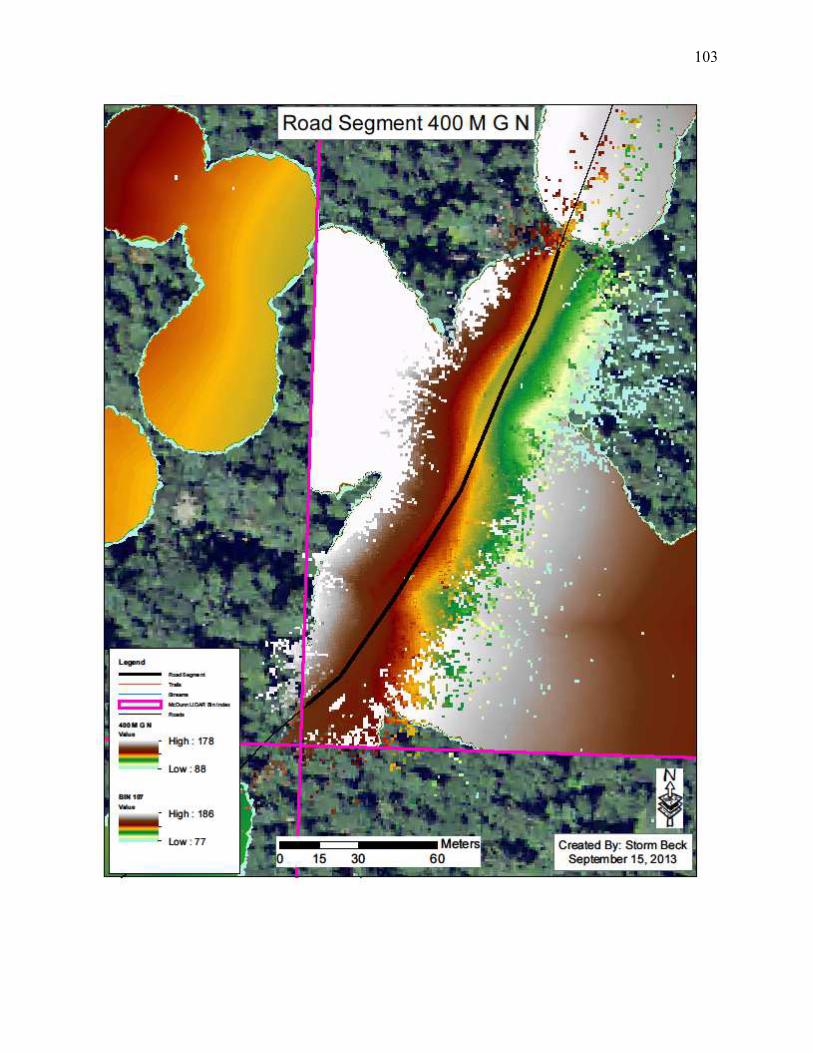
103

104

105

106

107
Appendix C
Road Profiles

108
289.00
290.00
291.00
292.00
293.00
294.00
295.00
-15.00 -10.00 -5.00 0.00 5.00 10.00 15.00
Ele
va
tio
n (
m)
Profile Distance (m)
Terrestrial vs Aerial
Profile 35
260 O G Y
Terrestrial
Aerial
280.00
281.00
282.00
283.00
284.00
285.00
286.00
-15.00 -10.00 -5.00 0.00 5.00 10.00 15.00
Ele
va
tio
n (
m)
Profile Distance (m)
Terrestrial vs Aerial
Profile 15
260 O G Y
Terrestrial
Aerial

109
296.0
297.0
298.0
299.0
300.0
301.0
302.0
-10.0 -5.0 0.0 5.0 10.0
Ele
va
tio
n (
m)
Profile Distance (m)
Terrestrial vs Aerial
Profile 15
260 O G Y 2
Terrestrial
Aerial
294.0
295.0
296.0
297.0
298.0
299.0
300.0
301.0
302.0
303.0
-10.0 -5.0 0.0 5.0 10.0
Ele
va
tio
n (
m)
Profile Distance (m)
Terrestrial vs Aerial
Profile 10
260 O G Y 2
Terrestrial
Aerial

110
176
178
180
182
184
186
188
-15 -10 -5 0 5 10 15
Ele
va
tio
n (
m)
Profile Distance (m)
Terrestrial vs Aerial
Profile 35
400 C G Y
Terrestrial
Aerial
172
174
176
178
180
182
184
-15 -10 -5 0 5 10 15
Ele
va
tio
n (
m)
Profile Distance (m)
Terrestrial vs Aerial
Profile 20
400 C G Y
Terrestrial
Aerial

111
141
142
143
144
145
146
147
148
-15 -10 -5 0 5 10 15
Ele
va
tio
n (
m)
Profile Distance (m)
Terrestrial vs Aerial
Profile 30
400 M G N
Terrestrial
Aerial
136
138
140
142
144
146
148
-15 -10 -5 0 5 10 15
Ele
va
tio
n (
m)
Profile Distance (m)
Terrestrial vs Aerial
Profile 5
400 M G N
Terrestrial
Aerial
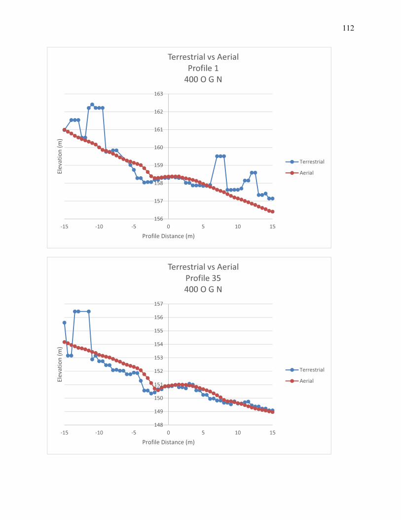
112
156
157
158
159
160
161
162
163
-15 -10 -5 0 5 10 15
Ele
va
tio
n (
m)
Profile Distance (m)
Terrestrial vs Aerial
Profile 1
400 O G N
Terrestrial
Aerial
148
149
150
151
152
153
154
155
156
157
-15 -10 -5 0 5 10 15
Ele
va
tio
n (
m)
Profile Distance (m)
Terrestrial vs Aerial
Profile 35
400 O G N
Terrestrial
Aerial
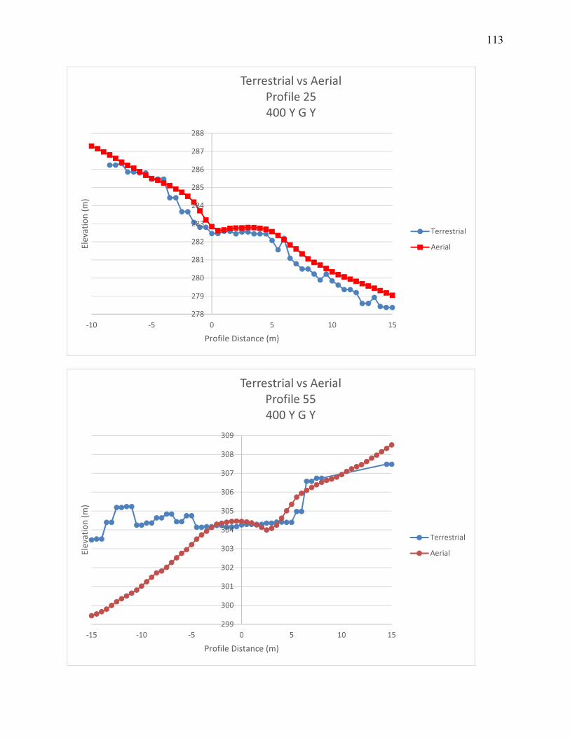
113
278
279
280
281
282
283
284
285
286
287
288
-10 -5 0 5 10 15
Ele
va
tio
n (
m)
Profile Distance (m)
Terrestrial vs Aerial
Profile 25
400 Y G Y
Terrestrial
Aerial
299
300
301
302
303
304
305
306
307
308
309
-15 -10 -5 0 5 10 15
Ele
va
tio
n (
m)
Profile Distance (m)
Terrestrial vs Aerial
Profile 55
400 Y G Y
Terrestrial
Aerial

114
137.00
137.10
137.20
137.30
137.40
137.50
137.60
137.70
137.80
137.90
138.00
-15.0 -10.0 -5.0 0.0 5.0 10.0 15.0
Ele
va
tio
n (
m)
Profile Distance (m)
Terrestrial vs Aerial
Profile 30
410 O D Y
Terrestrial
Aerial
267
267.5
268
268.5
269
269.5
270
-15 -10 -5 0 5 10 15
Ele
va
tio
n (
m)
Profile Distance (m)
Terrestrial vs Aerial
Profile 15
420 O G N
Terrestrial
Aerial
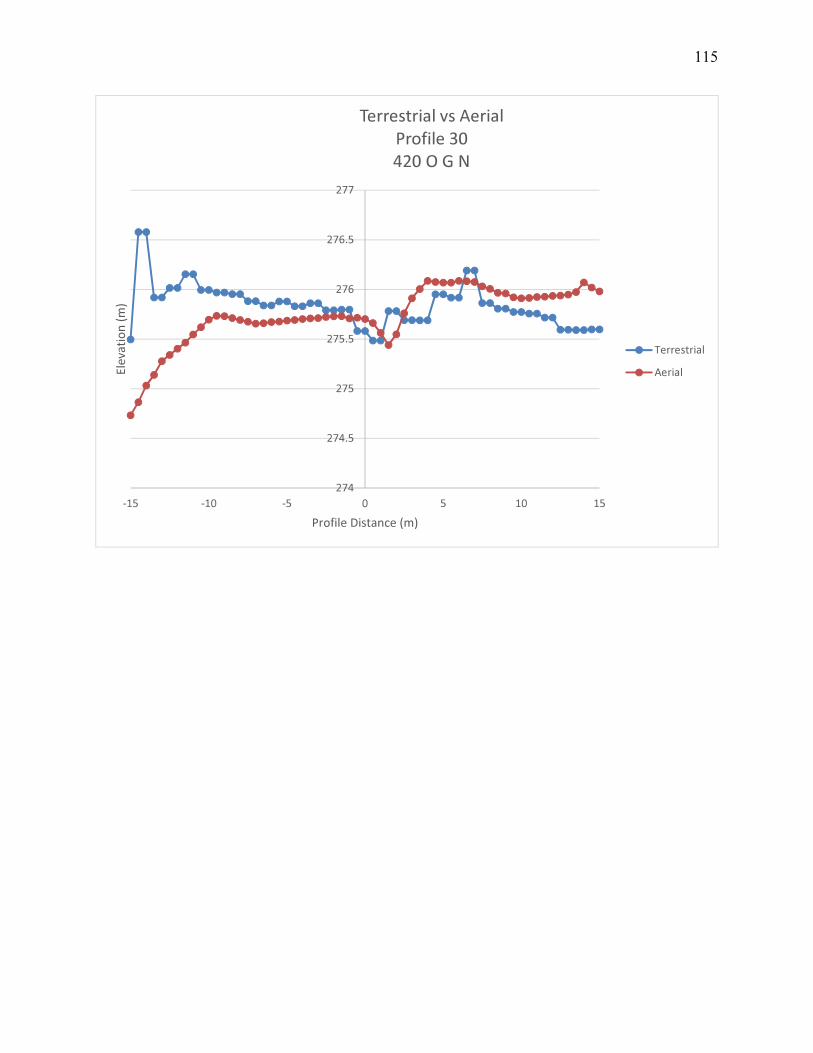
115
274
274.5
275
275.5
276
276.5
277
-15 -10 -5 0 5 10 15
Ele
va
tio
n (
m)
Profile Distance (m)
Terrestrial vs Aerial
Profile 30
420 O G N
Terrestrial
Aerial

116
Appendix D
Off-Tracking Model Comparison

117
When assessing the accessibility of vehicles throughout the transportation network the road
geometry that is being used to assess the vehicles would need to be of a certain quality. The
needed quality of the road geometry is dependent on vehicle type being assessed. This is
identified when comparing the various off-tracking methods. Six different off-tracking methods
were used to evaluate two different vehicle accessibility on a simple curve. The off-tracking
models that were used were the BLM’s minimum lane width calculation (Cain and Langdon,
1982), Glauz and Harwood’s off-tracking equation (Glauz and Harwood, 1991), a computer off-
tracking simulation called AUTOTURN (Carrasco, 1992), another computer off-tracking
simulation called OFFTRACK (Erkert et al., 1989), and the deep curve calculation. The vehicles
that were evaluated were a standard stinger-steered log truck and a stinger-steered pole truck.
The simple curve that was used to compare the methods was a 22.56m radius curve, with a delta
angle of 89.4 degrees, and road width of 4.26m and 1.82m of curve widening. The standard
stinger-steered log truck and the stinger-steered pole truck that was used in this analysis are
documented in Table D.1. The definitions of the vehicle measurements are shown in Figure
D.0.1.
Table D.1. Vehicle Configurations, L3 is an estimate of the extended reach (all measurements
are in meters).
Standard Log
Truck
Pole Log
Truck
L1 6.10 6.10
L2 3.05 5.18
L3 5.47 12.20
Radius 22.56 22.56
Delta 89.4˚ 89.4˚
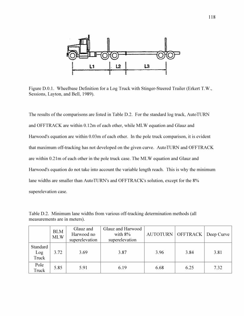
118
Figure D.0.1. Wheelbase Definition for a Log Truck with Stinger-Steered Trailer (Erkert T.W.,
Sessions, Layton, and Bell, 1989).
The results of the comparisons are listed in Table D.2. For the standard log truck, AutoTURN
and OFFTRACK are within 0.12m of each other, while MLW equation and Glauz and
Harwood's equation are within 0.03m of each other. In the pole truck comparison, it is evident
that maximum off-tracking has not developed on the given curve. AutoTURN and OFFTRACK
are within 0.21m of each other in the pole truck case. The MLW equation and Glauz and
Harwood's equation do not take into account the variable length reach. This is why the minimum
lane widths are smaller than AutoTURN's and OFFTRACK's solution, except for the 8%
superelevation case.
Table D.2. Minimum lane widths from various off-tracking determination methods (all
measurements are in meters).
BLM
MLW
Glauz and
Harwood no
superelevation
Glauz and Harwood
with 8%
superelevation
AUTOTURN OFFTRACK Deep Curve
Standard
Log
Truck
3.72 3.69 3.87 3.96 3.84 3.81
Pole
Truck 5.85 5.91 6.19 6.68 6.25 7.32

119
Table D.3. Statistics for the minimum lane widths (all measurements are in meters).
Average Standard Deviation
Standard Log Truck 3.82 0.10
Pole Truck 6.37 0.55
The average minimum lane widths are shown in Table D.3. The average minimum lane widths
were 3.82m and 6.37m for the standard log truck and pole truck case, respectively. It has been
observed that when log truck drivers are driving on forest roads they do not drive on a simple
radius curve, they swing to the outside of the curve during the traverse of a curve. Even with
these different off-tracking models, a vehicle may be able to navigate the curve when the
equation says otherwise. This is solely based on the drivers experience and aptitude at driving
on forest roads.
Literature Cited
Cain, C, and Langdon J. A. "A Guide for Determining Minimum Road Width on Curves for
Single-Lane Forest Roads." Engineering Field Notes. Vol. 14. USDA Forest Service,
April-June 1982.
Carrasco, Milton S. E. "Computerized Vehicle-Turning Simulation- An Interactive Application."
M.E., Civil Engineering, The University of Calgary, Calgary, Alberta, 1992.
Erkert, Thomas W., Sessions, John, Layton, Layton D., and Bell, Chris A. "Computer Simulation
of Offtracking of Truck and Trailer Combinations using Forest Raods." M.S. Thesis,
Department of Civil Engineering, Oregon State University, Corvallis, 1989, 98.
Glauz, William D., and Hardwood, Douglas W. "Superelevation and Body Roll Effects on
Offtracking of Large Trucks." Transportation Research Record 1303, 1991: 10.