engineering recommendation erec s34 draft issue 3 2016 … · 80 formula p4 touch voltage within...
TRANSCRIPT

PRODUCED BY THE OPERATIONS DIRECTORATE OF ENERGY NETWORKS ASSOCIATION
www.energynetworks.org
Engineering Recommendation EREC S34
Draft Issue 3 2016
A GUIDE FOR ASSESSING THE RISE OF EARTH POTENTIAL AT ELECTRICAL INSTALLATIONS

ENA Engineering Recommendation EREC S34 Draft November 2016
Page 2
<Insert publication history here, e.g. “First published, December, 2011”>
Amendments since publication
Issue Date Amendment
2 Draft 01-2017 E.g. Annex X introduced, equation sss revised, etc.
Alignment with 50522 and latest revisions of BS7430 and ENA TS 41-24. New equations introduced.
© 2014 Energy Networks Association
All rights reserved. No part of this publication may be reproduced, stored in a retrieval system or transmitted in any form or by any means, electronic, mechanical, photocopying, recording or otherwise, without the prior written consent of Energy Networks Association. Specific enquiries concerning this document should be addressed to:
Operations Directorate Energy Networks Association 6th Floor, Dean Bradley House
52 Horseferry Rd London
SW1P 2AF
This document has been prepared for use by members of the Energy Networks Association to take account of the conditions which apply to them. Advice should be taken from an appropriately qualified engineer on the suitability of this document for any other purpose.

ENA Engineering Recommendation EREC S34 Draft November 2016
Page 3
Contents 1
Introduction .......................................................................................................................... 10 2
1. Scope ............................................................................................................................ 10 3
2. Normative references ..................................................................................................... 10 4
3. Terms and definitions ..................................................................................................... 11 5
3.1 Symbols used ....................................................................................................... 11 6
3.2 Formulae used for calculating earth installation resistance for earthing 7 studies .................................................................................................................. 11 8
3.3 Description of system response during earth fault conditions ................................ 12 9
4. Earth fault current studies .............................................................................................. 14 10
4.1 Earth fault current ................................................................................................. 14 11
4.2 Fault current analysis for multiple earthed systems ............................................... 14 12
4.3 Induced currents in parallel conductors ................................................................. 14 13
4.3.1 Simple circuit representation for initial estimates ....................................... 15 14
4.3.2 More realistic circuit representation to improve the accuracy of 15 calculations ............................................................................................... 15 16
4.3.3 Amending calculations to account for increased ground return 17 current in single core circuits that are not in flat or trefoil touching 18 arrangement.............................................................................................. 16 19
5. EPR impact calculations ................................................................................................ 17 20
5.1 Calculation of touch potentials .............................................................................. 17 21
5.2 Calculation of step potentials ................................................................................ 17 22
5.3 Surface Potential contours .................................................................................... 18 23
5.4 Transfer potential to LV systems where the HV and LV earthing are 24 separate. ............................................................................................................... 18 25
5.4.1 Background ............................................................................................... 18 26
5.4.2 Basic theory .............................................................................................. 18 27
5.5 Risk assessment methodology.............................................................................. 21 28
5.6 Methods of optimising the design (first draft) ......................................................... 21 29
5.6.1 More accurate evaluation of fault current .................................................. 21 30
5.6.2 Reducing the overall earth impedance ...................................................... 21 31
5.6.3 Reducing the touch potential within the installation ................................... 21 32
6. Case study examples ..................................................................................................... 22 33
6.1 Case Study 1: Overhead line fed 33kV substation (33kV fault at Substation 34 B) .......................................................................................................................... 22 35
6.1.1 Earth resistance calculations ..................................................................... 23 36
6.1.2 Calculation of Fault Current and Earth Potential Rise ................................... 27 37
6.1.3 Calculation of touch potentials ..................................................................... 28 38
6.1.4 External touch potential at the edge of the electrode ................................. 28 39
6.1.5 Touch potential on fence ........................................................................... 30 40
6.1.5.1 Internal Touch Potentials ............................................................ 30 41
6.1.6 Calculation of external voltage impact contours ........................................ 30 42

ENA Engineering Recommendation EREC S34 Draft November 2016
Page 4
6.2 Case study 2 (33kV fault at substation B) ............................................................. 31 43
6.1.7 Resistance calculations ............................................................................. 31 44
6.1.8 Calculation of Fault Current and Earth Potential Rise ................................ 31 45
6.3 Case study 3 (33kV fault at Substation B, fed from a mixed cable and OHL 46 circuit) ................................................................................................................... 33 47
6.3.1 Resistance calculations ................................................................................ 33 48
6.3.1 Calculation of Fault Current and Earth Potential Rise ................................... 34 49
6.4 Case study 4 (Multiple neutrals) ............................................................................ 36 50
6.4.1 Introduction .................................................................................................. 36 51
6.4.2 Case Study Arrangement ............................................................................. 36 52
6.4.3 Case study data ........................................................................................... 37 53
6.4.4 Treatment of neutral current ......................................................................... 38 54
6.4.5 Fault current distribution ............................................................................... 38 55
6.4.6 Earth potential rise ....................................................................................... 39 56
6.5 Case study 5 (11kV Substation and LV earthing interface) ................................... 40 57
6.5.1.2 Surface Current Density ........................................................................... 42 58
6.5.2 Design Option 2 ................................................................................................... 43 59
APPENDICES ...................................................................................................................... 45 60
APPENDIX A – Symbols used within formulae ..................................................................... 46 61
APPENDIX B – Formulae ..................................................................................................... 50 62
6.6 Earth resistance formulae (R) ............................................................................... 50 63
Formula R1 Rod electrode .................................................................................... 50 64
Formula R2 Plate electrode (mainly used for sheet steel foundations) .................. 50 65
Formula R3 Ring electrode ................................................................................... 51 66
Formula R4 Grid/mesh resistance ......................................................................... 51 67
Formula R5 Group of rods around periphery of grid .............................................. 51 68
Formula R6 Combined grid and rods (rods on outside only) ................................. 53 69
Formula R7 Strip/tape electrode ........................................................................... 53 70
Formula R8 Ladder networks ................................................................................ 55 71
Formula R9 Accounting for proximity effects ......................................................... 56 72
Formula R10 Overall earth resistance ................................................................... 57 73
Formula C1 Current rating formula ........................................................................ 57 74
Formula C2 Limit of Surface Current Density formula ........................................... 58 75
6.7 Surface potential formulae (P) .............................................................................. 59 76
Formula P1 External touch potential at the edge of the electrode ......................... 59 77
Formula P2 External ‘Touch’ potential at the fence ............................................... 60 78
Formula P3 External touch potential at fence with external buried peripheral ........ 60 79
Formula P4 Touch voltage within grid (from IEEE80) ............................................ 61 80
Formula P5 Step voltage on outside edge of grid .................................................. 62 81
Formula P6 Voltage profile around earth electrode ............................................... 62 82
Formula P7 Calculation of specific external potential contours ............................. 64 83
APPENDIX C – Earthing design methodology ...................................................................... 65 84

ENA Engineering Recommendation EREC S34 Draft November 2016
Page 5
APPENDIX D – Formulae for determination of ground return current for earth faults on 85 metal sheathed cables ................................................................................................... 65 86
APPENDIX E – Ground current for earth faults on steel tower supported circuits with 87 an aerial earthwire ......................................................................................................... 73 88
APPENDIX F – Chart to calculate resistance of horizontal electrode .................................... 74 89
APPENDIX G – Chain impedance of standard 132kV earthed tower lines ........................... 76 90
APPENDIX H – Sample calculations showing the effect on the ground return current 91 for change in the separation distance between three single core cables laid flat or 92 in trefoil .......................................................................................................................... 77 93
APPENDIX I – Transfer potential to distributed LV systems ................................................. 84 94
I.1 Background ............................................................................................... 84 95
I.2 Examples .................................................................................................. 84 96
I.3 Discussion ................................................................................................ 86 97
I.4 Application to real systems ........................................................................ 87 98
I.5 Worked examples ..................................................................................... 87 99
Bibliography ......................................................................................................................... 90 100
101

ENA Engineering Recommendation EREC S34 Draft November 2016
Page 6
Figures 102
Figure 3-1 - Earth fault at an installation which has an earthed tower line supply ................. 12 103
Figure 3.2 Equivalent circuit for analysis .............................................................................. 13 104
Figure 5.1 Surface potential near a simple HV and LV electrode arrangement ..................... 19 105
Figure 5.2 Equivalent Circuit for Combined LV Electrodes A & B ......................................... 20 106
Figure 6.1 Supply arrangement for case study 1 ................................................................. 22 107
Figure 6.2 Substation B basic earth grid .............................................................................. 23 108
Figure 6.3 Substation B basic earth grid and rods ............................................................... 24 109
Figure 6.4 Substation B earth grid with rods and rebar ........................................................ 26 110
Figure 6.5 Supply arrangement for case study 2 .................................................................. 31 111
Figure 6.6 Supply arrangement for case study 3 .................................................................. 33 112
Figure 6.7 Case study arrangement ..................................................................................... 37 113
Figure H.1 Cross-sectional view for Cable 3 ......................................................................... 79 114
Figure H.2 Circuit used for analysis purposes ...................................................................... 79 115
Figure H.3 Ground return current (IES) as a percentage of (IF) against circuit length for 116 different 132kV cable installation arrangements .......................................... 81 117
Figure H.4 Ground return current (IES) as a percentage of (IF) against circuit length for 118 different 11kV cable installation arrangements ............................................ 83 119
Figure I.1 Example – Two Electrodes of Equal Resistance ................................................... 84 120
Figure I.2 Example - Two Electrodes of Unequal Resistance ............................................... 86 121
122
Tables 123
124
Table 6.2 EPR for different grid arrangements .................................................................... 28 125
Table 6.4 Data for fault current distribution and EPR Calculations ........................................ 32 126
Table 6.5 Data for fault current distribution and EPR calculation ........................................ 34 127
Table 6.6 Case study 3, input data and results for initial part of circuit ................................ 35 128
Table 6.7 Case study short-circuit data .............................................................................. 37 129
Table 6.8 Sum of contributions to earth fault current ........................................................... 38 130
Table 6.9 Case study information for fault current distribution calculations ......................... 39 131
Table 6.10 Calculated ground return current ....................................................................... 39 132
Table 6.11 Design Option 1, Input Data and Results ........................................................... 42 133
Table 6.12 Design Option 2, Input Data and Results ........................................................... 44 134
Table B.1 Approximate effective lengths for a single earth wire, tape or PILCSWA 135 cable ........................................................................................................... 54 136
Table B.3 Proximity effect of electrodes run in parallel (calculated using computer 137 software) ..................................................................................................... 57 138
Table D.1 Self and mutual impedances for a sample of distribution cables .......................... 71 139
Table H.1 Technical details of cables modelled .................................................................... 77 140

ENA Engineering Recommendation EREC S34 Draft November 2016
Page 7
Table H.2 The geometric placement of cables ...................................................................... 78 141
Table H.3 Effect of physical cable arrangement on ground return current IES for 132 kV 142 cables .......................................................................................................... 83 143
Table H.4 Effect of physical cable arrangement on ground return current IES for 11kV 144 cables .......................................................................................................... 83 145
146

ENA Engineering Recommendation EREC S34 Draft Issue 2 2014
Page 8
Foreword
This Engineering Recommendation (EREC) is published by the Energy Networks Association (ENA) and comes into effect from <Month, 2014>. It has been prepared under the authority of the ENA Engineering Policy and Standards Manager and has been approved for publication by the ENA Electricity Networks and Futures Group (ENFG). The approved abbreviated title of this engineering document is “EREC S34”, which replaces the previously used abbreviation “ER EREC S34”.

ENA Engineering Recommendation EREC S34 Draft Issue 2 2014
Page 9

ENA Engineering Recommendation EREC S34 Draft Issue 2 2014
Page 10
Introduction
This Engineering Recommendation is the technical supplement to TS 41-24 (2017), providing formulae, guidelines and examples of the calculations necessary to estimate the technical parameters associated with Earth Potential Rise (EPR).
TS 41-24 provides the overall rules, the design process, safety limit values and links with legislation and other standards.
1. Scope
This document describes the basic design calculations and methods used to analyse the performance of an earthing system and estimate the earth potential rise created, for the range of electrical installations within the electricity supply system in the United Kingdom, as catered for in TS 41-24. Modification to the calculations and methods may be necessary before they can be applied to rail, industrial and other systems.
2. Normative references
ENA TS 41-24 contains the main list of reference documents. Only reference documents used for EREC S34 and not listed in TS 41-24 are shown below.
Standards:
BS EN 50522: 2010: Earthing of power installations exceeding 1kV a.c.
ENA TS 41-24 (2016): Guidelines for the Design, Installation, Testing and Maintenance of Main Earthing Systems in Substations.
BS EN 60909-3: Short-circuit currents in three-phase a.c. systems. Currents during two separate simultaneous line-to-earth short-circuits and partial short-circuit currents flowing through earth
Other publications
To be added later • Align with bibliography

ENA Engineering Recommendation EREC S34 Draft Issue 2 2014
Page 11
3. Terms and definitions
3.1 Symbols used
Symbols or a similar naming convention to BS EN 50522 have been used and they are set out in Appendix A. Where these differ from the symbols used in earlier versions of this document, the previous symbols are shown alongside the new ones, to assist when checking previous calculations and formulae.
Note: Some equations taken from other standards have definitions that may not be consistent with the main body of this document – e.g. equation P4 has alternate definitions for some of the parameters. These have been retained to avoid the need for alternative definitions and to allow easy cross reference with source material.
3.2 Formulae used for calculating earth installation resistance for earthing studies
The most common formulae for power installations are included in Appendix B. These are generally used to calculate the resistance of an earth electrode system comprising of horizontal and/or vertical components or potentials at points of interest.
When using formulae to calculate earth resistances, caution is necessary, because they do not normally account for proximity effects or the longitudinal impedance of conductors.
For first estimates, the overall impedance 𝑍𝐸 of separate electrodes with respect to reference earth, is taken as the sum of their separate values in parallel. For the example shown in Figure 3-1, this would be:
𝑍𝐸 = (1
𝑅𝐸𝑆+
1
𝑍𝐶𝐻1+
1
𝑍𝐶𝐻2+ ⋯)
−1
(see Appendix A for description of symbols used)
In reality, 𝑍𝐸 will be higher if the separate electrodes are close enough that there is significant interaction between them (proximity effect). Proximity effects can be accounted for in most advanced software packages. When relying on standard formulae, the following techniques can
help to account for proximity when calculating 𝑍𝐸:
Include any radial electrodes that are short in relation to the substation size, into the overall calculation of the earth grid resistance.
For radial spur electrodes or cables with an electrode effect, assume the first part of its length is insulated over a distance similar to the substation equivalent diameter. Calculate the earth resistance of the remainder of the electrode/cable and add the longitudinal impedance of the insulated part in series.
For a tower line, assume that the line starts after one span of overhead earthwire (the longitudinal impedance of this earthwire/span would be placed in series with the tower line chain impedance).
A value of soil resistivity is needed and for the formula in Appendix B, this must be a uniform equivalent (see ENA TS 41-24, Section 8.1.) For soils that are clearly of a multi-layer structure with significant resistivity variations between layers, the formulae must be used with caution and it is generally better to use dedicated software that accounts for this to provide results of the required level of accuracy.

ENA Engineering Recommendation EREC S34 Draft Issue 2 2014
Page 12
3.3 Description of system response during earth fault conditions
Figure 3-1 - Earth fault at an installation which has an earthed tower line supply
The arrangement shown in Figure 3.1 is based upon the example described in BS EN 50522 and will be explained and developed further in this document. The EPR is the product of earth electrode impedance and the current that flows through it into the soil and back to its remote source. The description below is to show how the fault current and associated impedances are dealt with to arrive at the components that are relevant to the EPR.
The installation is a ground-mounted substation that is supplied or looped into an overhead line circuit that is supported on steel towers and has an over-running earthwire. In this simplified example, for clarity currents are shown only on one of the infeed circuits, and flow in one earth wire only. It is also assumed that each tower line supports only one (three phase) circuit.
The fault condition is a high voltage phase insulation failure to earth within the substation. It is possible to model this situation with computer software such that all of the effects are summated, calculated and results presented together. For traditional analysis in this standard, the effects are decoupled as described below.
The total earth fault current at the point of fault (𝐼𝐹 ) that will flow into the earth grid and associated components would be reduced initially by two components.
The first component is that passing through the transformer star point earth connection (𝐼𝑁) and returning to source via the unfaulted phase conductors. For systems that are normally multiply earthed, i.e. at 132kV and above, the total current excluding the 𝐼𝑁 component is normally calculated by summating the currents in all three phases (3𝐼0) vectorially. The
process is further described in Case Study 4. For lower voltage distribution systems, 𝐼𝑁 is normally zero or sufficiently low to be ignored in calculations.
The second reduction is due to coupling between the faulted phase and continuous earth
conductor (see 4.3 below.) This part of the current is normally pre-calculated for
standard line arrangements or can be individually calculated from the support structure
geometry, conductor cross section and material. A similar procedure is followed for a
Reference Earth
IF
UE
IN
IES
RET RES RET
3I0
(1 - rE) 3I0
Source
ZCH2ZCH1
IET1 IET2

ENA Engineering Recommendation EREC S34 Draft Issue 2 2014
Page 13
buried cable. Another approach is to use a reduction factor (termed rE) based on the
specific circuit geometry and material.
Once these components have been removed, the situation is shown in Figure 3.2. The earth
current (𝐼𝐸) is treated as flowing into the earth network, which in this example contains the substation earth grid (resistance 𝑅𝐸𝑆) and two ‘chain impedances’, of value 𝑍𝐶𝐻1 and 𝑍𝐶𝐻2. The two chain impedances are each a ladder network consisting of the individual tower footing
resistance 𝑅𝐸𝑇 in series with the longitudinal impedance of each span of earthwire. They are treated as being equal if they have more than 20 similar towers in series and are in soil of
similar resistivity. The overall impedance of the electrode network is 𝑍𝐸 and the current (𝐼𝐸) flowing through it creates the Earth Potential Rise (𝑈𝐸). The analysis of the performance of the system described follows the process shown in the design flow diagram (Appendix C.) The case studies in section 6 illustrate this process for a number of examples of increasing complexity.
Figure 3.2 Equivalent circuit for analysis
Earthing System
Reference Earth
UE
IE
IES
ZCH1 RES ZCH2
IET2IET1

ENA Engineering Recommendation EREC S34 Draft Issue 2 2014
Page 14
4. Earth fault current studies
This section describes how to use the fault current data (calculated using the methodology set out in BS EN 60909 and guidance from TS 41-24, Section 8.2) for earth potential rise purposes.
4.1 Earth fault current
Source earth fault current values (such as the upper limit with neutral earth resistors in place) may be used for initial feasibility studies, but for design purposes, the value used should be site specific, i.e. should account for the fault resistance and longitudinal phase impedance between the source and installation.
Once the fault current is known, the clearance time for a “normal protection” operation (as defined in TS 41-24), at this level of current should be determined and the applicable safety voltage limits obtained from TS 41-24, Section 6. This basis of a normal protection operation is used for the personnel protection assessment. Design measures should be included within installations to afford a higher level of protection to personnel in the event of a main protection failure.
For protection and telecommunication equipment immunity studies in distribution systems, the steady state RMS fault current values are normally used. At some installations, particularly where there are significant generation in-feeds, consideration should be given to sub-transient analysis. This is especially important where vulnerable equipment (such as a telephone exchange) is installed close to a generation installation.
For calculation of the EPR, it is the ground return component of the fault current (𝐼𝐸) that is of concern. On some transmission systems, this can be greater for a phase-phase-earth fault (compared to a straightforward phase-earth fault) and where applicable, this value should be used for the EPR calculation.
4.2 Fault current analysis for multiple earthed systems
The methodology followed in this document assumes that the earth fault current at the substation (possibly at a defined point in the substation) has been separately calculated using power system analysis tools, symmetrical components or equivalent methods. Depending upon the complexity of the study, the data required may be a single current magnitude or the three phase currents in all supply circuits in vector format.
4.3 Induced currents in parallel conductors
The alternating current that flows in a conductor (normally a phase conductor) will create a longitudinal emf in conductors that lie in parallel with it. These are typically cable metal screens (lead sheath, steel armour or copper strands), earthwires laid with the circuit, metal pipes, traction rails or the earthwires installed on overhead lines. This emf will increase from the point of its earth connection as a function of the length of the parallelism and other factors (such as the separation distance.) If the remote end of the parallel conductor is also connected to earth, then a current will circulate through it, in the opposite general direction to the inducing current.
The current that flows (returns) via the cable sheath or earthwire during fault conditions can be large and it has the effect of reducing the amount of current left to flow into the ground via the electrode system, resulting in a reduced EPR on it.
The following sections provide methods to account for these return currents.

ENA Engineering Recommendation EREC S34 Draft Issue 2 2014
Page 15
4.3.1 Simple circuit representation for initial estimates
For an overhead line with a single earthwire, or a single cable core and its earth sheath, the
formulae below approximate the ground return current (𝐼𝐸). The main assumption is that the circuit is long enough such that the combined value of the earthing resistances at each end of
the line are small compared with 𝑧𝑠 (earthwire impedance), or for cable, small compared with 𝑟𝑐 (cable sheath resistance).
For an overhead line:
𝐼𝐸 = 𝑘(𝐼𝐹 − 𝐼𝑁) where 𝑘 = (1 −𝑧𝑚𝑝,𝑠
𝑧𝑠)
Appendix E gives calculated values of 𝐼E presented as a percentage value of 𝐼𝐹, and phase
angle with respect to 𝐼𝐹 for a range of the most commonly used overhead line constructions at 132 kV, 275 kV and 400 kV.
For a single core cable:
𝐼𝐸 = 𝑘(𝐼𝐹 − 𝐼𝑁) where 𝑘 = (𝑟𝑐𝑧𝑐
)
The equations are not sufficiently accurate for short circuits (less than 1km). The results are sensitive to even relatively low values of terminal (electrode) resistance. For most practical situations the more detailed approach presented in Section 4.3.2 will be required.
4.3.2 More realistic circuit representation to improve the accuracy of calculations
More complete formulae are presented in Appendix D. They require a number of circuit and cable specific factors to provide sufficiently accurate results. These have been included in Table A4.1 (Appendix D), for a representative sample of cables.
The case studies have been selected to show how to use the formulae and calculations for a range of different scenarios. The calculations generally provide results that are conservative, because parallel circuit earthwires or cables are not included in the circuit factors. The parallel earthwires or cables can be included in the circuit factors and their use in the formulae of Appendix D will then provide more accurate results.
Where single core cables are used for three phase circuits, the calculations are based upon them being installed in touching trefoil formation, earthed at each end. Where the cables are not in this arrangement, the results may be optimistic and correction factors need to be considered, (see. 4.3.3 and Appendix H.)
The formulae and calculations are sufficiently accurate for use at 11kV and 33kV on radial circuits. Circuit factors have not been included for 66kV cables because so little of this is present within DNOs, typically only for initial lengths of predominantly overhead line circuits. First estimates for these cables can be made using a similar 33kV cable.
At 132kV, the formulae and calculations are sufficiently accurate for use in feasibility studies, especially for single end fed “all cable” circuits. They should normally provide conservative results. This is because the circuit factors calculated are for the cable construction that provides the highest ground return current, due for example to having the highest longitudinal sheath impedance and/or weakest mutual impedance between the faulted and return conductors. This would result from a cable with the smallest cross section area of sheath or the least conductive material (such as all lead rather than composite, aluminium or stranded copper) and thicker insulation (older type cables which subsequently have a slightly weaker mutual coupling between the core and sheath). If further refinement or confidence is required, the circuits

ENA Engineering Recommendation EREC S34 Draft Issue 2 2014
Page 16
should be modelled with the appropriate level of detail and the work would normally show that a lower ground return current is applicable (i.e. more current returning via the cable screens or metallic routes.)
The formulae and calculations cater for simple overhead line circuits where there is no associated earthwire. For steel tower supported circuits that have an over-running earthwire, account is made of the induced current return by using the table in Appendix E. Circuits that contain both underground cable and earthed overhead tower line construction are not presently addressed and need to be analysed on a site specific basis.
4.3.3 Amending calculations to account for increased ground return current in single core circuits that are not in flat or trefoil touching arrangement
The fault current calculations described in this document for single core cable have assumed that the cables are earthed at each end and in touching trefoil formation.
In many practical situations, the cables are separated by a nominal distance, either deliberately (to reduce heating effects) or inadvertently (for example when installed in separate ducts.)
When the distance between the individual cables is increased, the coupling between the faulted and other two cables is reduced. This in turn results in more current flowing through the local electrodes (RB and RA) and an increase in the EPR at each point.
Some fault current studies for 11kV and 132kV cables where the cables are in touching trefoil, touching flat or the spacing is 3 x D (i.e. 3 x the cable diameter) are included in Appendix H.
These show that, compared to touching trefoil, the ground return current component increases for the other arrangements as:
The cable length increases
The cable screen cross sectional area (or conductivity) increases
For a flat arrangement of 3 x D spacing, the ground return current is seen to increase by up to about 6% to 7%. Accordingly, if the cables are not touching, the ground return current and EPR may be adjusted by this amount or a more accurate amount deduced from the information in Appendix H or more detailed site specific analysis. If this effect is not accounted for, the results will be optimistic.

ENA Engineering Recommendation EREC S34 Draft Issue 2 2014
Page 17
5. EPR impact calculations
5.1 Calculation of touch potentials
When developing formulae for calculating the value of 'touch' potentials, it is normal practice to refer these calculations to the potential of the natural ground surface of the site. From the safety aspect these calculated values are then compared with the appropriate safe value given in TS 41-24 which takes account of any footwear or ground covering resistance (e.g. chippings or concrete). It is important, therefore, to appreciate that the permissible safe value of 'touch' potential, as calculated in this section, will differ depending on the ground covering, fault clearance time and other factors prevailing at the site.
The developed formulae are not rigorous but are based on the recognised concept of integrating the voltage gradient, given by the product of soil resistivity and current density through the soil, over a distance of one metre. Experience has shown that the maximum values of 'touch' potential normally occur at the external edges of an earth electrode. For a grid electrode this potential is increased by the greater current density transferring from the electrode conductors to ground around the periphery of the grid as compared with that transferring in the more central parts. These aspects have been taken into account in the formulae firstly for 'touch' potential and secondly for the length of electrode conductor required to ensure a given 'touch' potential is not exceeded.
Formulae are provided in Appendix B to provide the following:
• External touch potential at the edge of the electrode (separately earthed fence) – Formula P1.
• External touch potential at the fence (separately earthed fence) – P2. • External touch potential at fence where there is no external perimeter electrode (bonded
fence arrangement) – P1. • External touch potential at fence with external perimeter electrode 1m away (bonded fence
arrangement) – P3. • Touch voltage within substation earth grid – P4
5.2 Calculation of step potentials
The step potential is the potential difference between two points that are 1m apart. This can be derived as the difference in calculated surface potential between two points that are 1m apart (Appendix B Formula P5). Note that this equation loses accuracy within a few metres of the grid.
𝑈𝑣𝑠 =𝜌𝐼𝐹
2𝜋𝑟(arcsin
𝑟
𝑥− arcsin
𝑟+1
𝑥) where 𝑟 =
𝜌
4𝑅𝐸 [P5]

ENA Engineering Recommendation EREC S34 Draft Issue 2 2014
Page 18
5.3 Surface Potential contours
The EPR at the substation creates potentials in the soil external to the substation. Equation P7 in Appendix B can be used to provide an estimate of the distance to the contour of interest.
The formula is as below:
𝑍𝑥 = √𝐴
𝜋[(𝑠𝑖𝑛
𝑉𝑥 𝜋
2 𝑈𝐸)−1
− 1] [P7]
Where 𝑍𝑥 is the distance to the point from the edge of the grid to where the voltage is 𝑉𝑥, and A is the area of the grid in square metres.
As emphasised elsewhere in this document, this and other formulae are restricted in accuracy by their assumptions of a symmetrical electrode grid and uniform soil resistivity. More accurate plotting of contours is possible using computer software or site measurements.
5.4 Transfer potential to LV systems where the HV and LV earthing are separate.
5.4.1 Background
This issue predominantly concerns distribution substations (typically 11kV:LV in the UK) where the HV and LV earthing systems are separate. Another application is where an LV earthing system is situated within the zone of influence of a Primary Substation with a high EPR. Previous guidance was based upon the presence of a minimum ‘in ground’ separation between the two electrode systems being maintained (distances of between 3m and 9m have historically been used in the UK). Operational experience suggested that there were fewer incidents than would be expected when the separation distance had been encroached on multiply earthed (i.e. TNC-S or PME arrangements). Theoretical and measurement studies (reference xx – Davies/Baudin et al – see Bibliography) showed that the minimum separation distance is a secondary factor, the main ones being the size and separation distance to the dominant or average LV electrode (where there are many small electrodes rather than one or a few large ones). We refer to this as the ‘centre of gravity’ of the LV electrode system.
Further information, together with worked examples is given in Appendix I.
5.4.2 Basic theory
Equations are available Appendix B (P6) to calculate the surface potential a given distance away from an earth electrode. Three different electrode shapes are included as follows:
a) A hemispherical electrode at the soil surface b) A vertical earth rod c) An earth grid – approximated to a horizontal circular plate.
The surface potential calculated at a point using these formulae is equal to the transfer potential to a small electrode located at that point because an isolated electrode would simply rise to the same potential as the surrounding soil.
When two or more electrodes are connected together, previous investigations have shown that the transfer potential on the combined electrode is an ‘average’ of the potentials that would exist on the individual components. This ‘average’ was found to be ‘skewed’ towards the surface potentials on ‘dominant’ electrodes, i.e. those having a lower earth resistance due mainly to being larger.

ENA Engineering Recommendation EREC S34 Draft Issue 2 2014
Page 19
A simple method is required to explain and then account for this ‘averaging’ effect. Figure 5.1 shows a simple arrangement of a HV earth electrode and two nearby LV earth rods (A and B) which are representative of typical PME electrodes.
The three electrodes are located along a straight line and the soil surface potential profile along this route is also approximated in the figure.
Figure 5.1 Surface potential near a simple HV and LV electrode arrangement
When there is an EPR (Earth Potential Rise) on the HV Electrode the LV Electrodes, A and B will rise to the potential of the local soil, i.e. the surface potential. In Figure 5.1, these are defined as VA and VB. The LV Electrodes are clearly at different potentials and this depends on the distance away from the HV electrode.
Once A and B are connected together (for example by the sheath / neutral of an LV service cable) the potential on them will change to an ‘average’ value, between VA and VB. In simple cases where A and B are of a similar size (with the same earth resistance in soils of similar resistivity), the average potential is accurate but where electrodes A and B are of significantly different sizes the ‘average’ is ‘skewed’ towards the dominant one (the larger one, i.e. that has the lowest earth resistance).
The ‘averaging’ effect can be explained by considering an equivalent circuit for the combined LV electrodes as shown in Figure 5.2. VA and VB are the local soil surface potentials and VT is the overall potential on the combined LV electrode. Electrodes A and B have earth resistances of RA and RB respectively.
Distance
VB
VA
LV Electrode
B
LV Electrode
A
Soil
Surface
Potential
HV
Electrode
LV Electrode
A
VT
VB VA
RB RA
LV Electrode
B

ENA Engineering Recommendation EREC S34 Draft Issue 2 2014
Page 20
Figure 5.2 Equivalent Circuit for Combined LV Electrodes A & B
The circuit is a potential divider and the voltage on the combined LV electrode (VT) can be expressed by:
𝑉𝑇 =𝑉𝐴𝑅𝐵 + 𝑉𝐵𝑅𝐴
𝑅𝐴 + 𝑅𝐵
If the LV electrode earth resistances are equal (RA = RB) then this equation reduces to VT = (VA + VB)/2, i.e. the average of the two potentials.
Worked examples are given in Appendix I.

ENA Engineering Recommendation EREC S34 Draft Issue 2 2014
Page 21
5.5 Risk assessment methodology
The risk assessment process is described in detail in ENA TS 41-24. It should be used as a last resort only, and needs to be justified, e.g. when achieving safe (deterministic) touch and step potentials is not practicable and economical.
For UK electricity industry applications, the risk of ventricular fibrillation (or electrocution) is a function of three probabilities, i.e.:
P (Probability of ventricular fibrillation) = PF x PE x PFB
Where
PF : Probability of fault occurrence
PE : Probability of exposure
PFB: Probability of fibrillation
5.6 Methods of optimising the design (first draft)
Where the EPR is sufficient to create issues within or external to the substation, the following should be investigated and the most practicable considered for implementation.
5.6.1 More accurate evaluation of fault current
Does the value used, account for fault resistance and longitudinal circuit impedance? Have excessive factors for future fault current growth been used? For example, it may be more prudent to use the existing value and implement additional measures later, i.e. at the same time as the predicted increase in fault current.
5.6.2 Reducing the overall earth impedance
Can additional horizontal electrode be incorporated with new underground cable circuits?
Has the contribution of PILCSWA type cables in the vicinity been appropriately accounted for?
5.6.3 Reducing the touch potential within the installation
Can rebar or other non-bonded buried metalwork be connected to the electrode system?
Can other measures (such as physical barriers or isolation) be applied to certain areas?
Are the areas of high touch potential actually accessible?

ENA Engineering Recommendation EREC S34 Draft Issue 2 2014
Page 22
6. Case study examples
The five case studies demonstrate the differences in complexity and design philosophies involved when moving from an unearthed overhead supplied installation with a single supply through to a distribution or transmission installation that has several sources of supply. All case studies demonstrate the new design facilities that are expected at a modern installation, together with use of the fault current analysis formulae available with this document.
6.1 Case Study 1: Overhead line fed 33kV substation (33kV fault at Substation B)
A new 33kV substation is to be built as Substation B. It is supplied from Substation A via an unearthed wood pole supported line that terminates just outside the operational boundary of each substation. The new substation is assumed to consist of just three items of plant, (incoming, outgoing, and a power transformer), each on their own individual foundation slab. This is the most straightforward example to study and will be used to demonstrate both the modern design approach and methods of addressing touch potentials.
The approach used can be applied to similar arrangements at a range of voltage levels from 6.6kV to 66kV. At 6.6kV and 11kV, the substation would generally occupy a smaller area than in the examples shown.
This example considers a 33kV earth fault at Substation B on the incoming line termination as shown in the diagram below.
Figure 6.1 Supply arrangement for case study 1
(Overhead line fed substation)
For simplicity, all electrodes are assumed to be copper and have an equivalent circular diameter of 0.01m (the electrical properties of steel could be used for the reinforcing material). The soil resistivity is 75Ω·m and the 33kV fault current magnitude is limited to a maximum of 2kA by a neutral earth resistance connected to the 33kV winding neutral at Substation A.
Substation A is assumed to be an overhead fed 132/33kV substation with a measured earth resistance of 0.25Ω. The overhead line conductors between Substation A and B are assumed to be 185mm2 ACSR.
Table 6.1 provides the fault clearance time and associated touch voltage limits for 33kV earth faults at Substation B when fed from Substation A.
Earth Rods
Switchgear
Substation A
Earthing
System
Switchgear
Earthing
System 0.6m deep
Earth Rod
Switchgear
Substation B Line
termination Transformer

ENA Engineering Recommendation EREC S34 Draft Issue 2 2014
Page 23
Table 6.1 Fault clearance time and touch voltage limits
6.1.1 Earth resistance calculations
For this case, the land area is assumed to be fixed. The first calculation assumes a minimum earthing system consisting of a perimeter electrode 1m outside the foundation slabs and two cross members in-between the slabs (Fig.6.2). For the next iterations, ten vertical 3.6m rods are added (Fig.6.3) and then some horizontal rebar within each foundation slab (Fig.6.4).
Figure 6.2 Substation B basic earth grid
Using Formula R4 from Appendix B, as below:
𝑅𝐸 =
4𝑟+
𝐿𝐸
Where 𝐿𝐸 = length of buried conductor (not including rods);
𝑟 = √𝐴
𝜋
𝐴 = area of grid.
Substituting the values, as below:
𝑅𝐸 =75
4𝑟+
75
140
Where
33kV Fault
Clearance
Time (s)
Touch Voltage
Limit (V) Inside
Substation (75mm
chippings)
Touch Voltage
Limit (V) Outside
Substation (on
soil)
0.4 944 837
0.6m deep
Substation B
Earthing
System
20m
30m

ENA Engineering Recommendation EREC S34 Draft Issue 2 2014
Page 24
𝑟 = √𝐴
𝜋= √
600
𝜋= 13.8
𝑅𝐸 =75
55.3+
75
140
𝑅𝐸 = 1.89Ω
Adding the ten rods as below, each of 3.6m length and 16mm diameter, requires the use of the more detailed formula.
Figure 6.3 Substation B basic earth grid and rods
Using Formula R6 from Appendix B:
𝑅𝐸 =𝑅1𝑅2 − 𝑅12
2
𝑅1 + 𝑅2 − 2𝑅12
Note: This formula may not be valid for unconventional geometries in which case computer modelling should be used.
Earth Rods
0.6m deep

ENA Engineering Recommendation EREC S34 Draft Issue 2 2014
Page 25
Where:
𝑅1 = 𝑅𝐸𝑆 =
4𝑟+
𝐿𝐸
𝑅𝑅 =
2𝜋𝐿𝑅(𝑙𝑜𝑔𝑒
8𝐿𝑅
𝑑− 1)
𝑅2 = 𝑅𝐸𝑅 = 𝑅𝑅 (1 + 𝑘𝛼
𝑁)
𝛼 =𝜌
2𝜋𝑅𝑅𝑠
𝑅12 = 𝑅1 −
𝜋𝐿𝐸(𝑙𝑜𝑔𝑒
𝐿𝑅
𝑏− 1)
𝑅𝐸 = 𝑅1𝑅2 − 𝑅12
2
𝑅1 + 𝑅2 − 2𝑅12
Therefore:
𝑅1 =75
4 × 13.82+
75
140= 1.89Ω
𝑅𝑅 =75
2𝜋 × 3.6(log𝑒 (
8 × 3.6
0.016) − 1) = 21.6Ω
𝛼 =75
2𝜋 × 21.6 × 10= 0.055
𝑅2 = 21.6 × (1 + 4.9 × 0.055
10) = 2.74Ω
𝑅12 = 1.89 −75
𝜋 × 140(𝑙𝑜𝑔𝑒
3.6
0.01− 1) = 1.06Ω
𝑅𝐸 =1.89 × 2.74 − 1.062
1.89 + 2.74 − 2 × 1.06= 1.62Ω
𝐿𝐸 = Length of horizontal
electrode
𝐿𝑅 = Rod length; d=diameter. Valid
for d<<𝐿𝑅
𝑟 = √𝐴
𝜋
A = area of grid (m2)
𝑁 = total number of rods
k = 4.9 for 10 rods – see
Appendix B, formula R5
𝑠 = separation distance between
rods (m)
b = equivalent diameter of the circular earth electrode or the width of a tape electrode.
As can be seen, the rods have reduced the resistance to 1.62 Ω compared to 1.89 Ω without rods.

ENA Engineering Recommendation EREC S34 Draft Issue 2 2014
Page 26
For the final calculation, the rebar within the horizontal foundations have been approximated by the symmetrical meshes shown in Figure 6.4. For simplicity it is assumed that they have the same equivalent circular diameter as the copper conductor and the same electrical properties (Note 1).
Figure 6.4 Substation B earth grid with rods and rebar
The same formula (R6) and approach would be used as previously, except that the length of conductor is increased to include the amount of rebar modelled (786m total of rebar added to that of copper).
Using Formula R6 from Appendix B:
𝑅𝐸 =𝑅1𝑅2 − 𝑅12
2
𝑅1 + 𝑅2 − 2𝑅12
Re-Bar Re-Bar Re-Bar
0.6m deep
Earth Rods
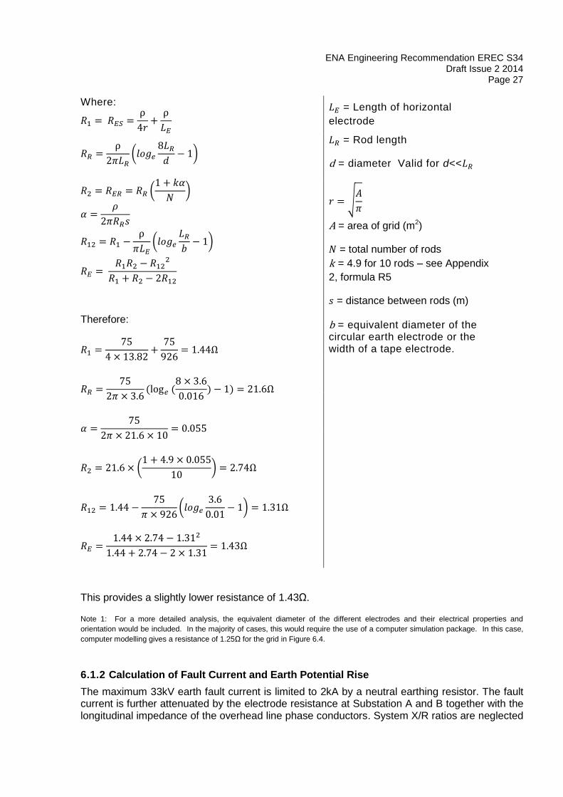
ENA Engineering Recommendation EREC S34 Draft Issue 2 2014
Page 27
Where:
𝑅1 = 𝑅𝐸𝑆 =
4𝑟+
𝐿𝐸
𝑅𝑅 =
2𝜋𝐿𝑅(𝑙𝑜𝑔𝑒
8𝐿𝑅
𝑑− 1)
𝑅2 = 𝑅𝐸𝑅 = 𝑅𝑅 (1 + 𝑘𝛼
𝑁)
𝛼 =𝜌
2𝜋𝑅𝑅𝑠
𝑅12 = 𝑅1 −
𝜋𝐿𝐸(𝑙𝑜𝑔𝑒
𝐿𝑅
𝑏− 1)
𝑅𝐸 = 𝑅1𝑅2 − 𝑅12
2
𝑅1 + 𝑅2 − 2𝑅12
Therefore:
𝑅1 =75
4 × 13.82+
75
926= 1.44Ω
𝑅𝑅 =75
2𝜋 × 3.6(log𝑒 (
8 × 3.6
0.016) − 1) = 21.6Ω
𝛼 =75
2𝜋 × 21.6 × 10= 0.055
𝑅2 = 21.6 × (1 + 4.9 × 0.055
10) = 2.74Ω
𝑅12 = 1.44 −75
𝜋 × 926(𝑙𝑜𝑔𝑒
3.6
0.01− 1) = 1.31Ω
𝑅𝐸 =1.44 × 2.74 − 1.312
1.44 + 2.74 − 2 × 1.31= 1.43Ω
𝐿𝐸 = Length of horizontal
electrode
𝐿𝑅 = Rod length
d = diameter Valid for d<<𝐿𝑅
𝑟 = √𝐴
𝜋
A = area of grid (m2)
𝑁 = total number of rods
k = 4.9 for 10 rods – see Appendix
2, formula R5
𝑠 = distance between rods (m)
b = equivalent diameter of the circular earth electrode or the width of a tape electrode.
This provides a slightly lower resistance of 1.43Ω.
Note 1: For a more detailed analysis, the equivalent diameter of the different electrodes and their electrical properties and
orientation would be included. In the majority of cases, this would require the use of a computer simulation package. In this case,
computer modelling gives a resistance of 1.25Ω for the grid in Figure 6.4.
6.1.2 Calculation of Fault Current and Earth Potential Rise
The maximum 33kV earth fault current is limited to 2kA by a neutral earthing resistor. The fault current is further attenuated by the electrode resistance at Substation A and B together with the longitudinal impedance of the overhead line phase conductors. System X/R ratios are neglected

ENA Engineering Recommendation EREC S34 Draft Issue 2 2014
Page 28
for simplicity. Table 6.2 provides the fault current and EPR corresponding to the earth resistances calculated in section 6.1.1.
Arrangement Resistance
(Ω)
Earth Fault Current at
Substation B*
(A)
EPR (V)
Basic grid 1.89 1447 2735
Grid & rods 1.62 1477 2393
Grid, rods & rebar
(using formula) 1.43 1499 2144
Grid, rods & rebar
(using computer
software for
comparison)
1.25 1521 1901
* For simplicity this has been calculated using an equivalent single phase circuit including the earth resistance at Substation A (0.25Ω), NER value (9.53Ω), circuit impedance (1.5Ω) and the earth resistance at Substation B from the table. These values would normally be available from power system short-circuit analysis software.
Note 1: Because there is an unearthed overhead line supply the calculated earth fault current is equal to the ground return current in this example.
Table 6.2 EPR for different grid arrangements
The addition of the rods and rebar have each reduced the resistance and EPR, but not dramatically. The site has an EPR that exceeds twice the acceptable touch voltage limit. It is therefore necessary to calculate the safety voltages and compare to touch voltage limits.
6.1.3 Calculation of touch potentials
Formula P1 estimates the touch potential one metre beyond the perimeter electrode. It is usually the case that provided the internal electrode has been correctly designed (with sufficient meshes), the touch potential here will exceed that anywhere within the grid area. Where the internal mesh is large the internal touch voltage at the center of the corner mesh may be approximated using Formula P4. For unusually shaped or non-symmetrical grids, computer software tools are needed for an accurate calculation.
The calculation procedure is as below:
For simplicity, the grid without foundation rebar is used, as in Figure 6.3. A single cross member is added later to give an initial estimate of the effect of the rebar.
6.1.4 External touch potential at the edge of the electrode
Using formula P1:

ENA Engineering Recommendation EREC S34 Draft Issue 2 2014
Page 29
𝑈𝑇 =𝑘𝑒 ∙ 𝑘𝑑 ∙ 𝜌 ∙ 𝐼
𝐿𝑇
𝑘𝑒 =1
𝜋(1
2𝑙𝑜𝑔𝑒
ℎ
𝑑+
1
2ℎ+
1
(0.5 + 𝐷)+
1
𝐷(1 − 0. 5𝑛−2))
ℎ = 0.6m, 𝑑 = 0.01m
𝐷 = average spacing between parallel grid conductors = (20m + 10m)/2 = 15m
𝑛 = (𝑛𝐴 × 𝑛𝐵)1
2⁄
Where 𝑛𝐴 = 2, 𝑛𝐵 = 4 (number of conductors – add definition if not in appendix)
𝑘𝑑 is a factor which modifies 𝑘𝑒 to allow for non-uniform distribution of electrode current and is given by:
𝑘𝑑 = (0.7 + 0.3𝐿𝑇
𝐿𝑝)
Where 𝐿𝑇 = total length of buried electrode conductor including rods if connected (176 m)
𝐿𝑝 = length of perimeter conductor including rods if connected (136 m)
𝜌 = 75 Ω·m
𝐼 = total current passing to ground through electrode (1477A)
UT(grid) = 648V
This reduces to 602V if an additional central cross member is added along the x axis (this adds 30m of electrode and provides a uniform separation between mesh conductors in each direction of 10m).
Where there are more cross members or to account for the rebar, the additional conductors are accounted for in the formula in a similar process to that above and will provide a lower touch potential.
For comparison purposes, when the grids are modelled using computer software, the touch potentials are:
Basic grid (plus rods), touch voltage 1m from the edge of the grid varies from 24% of the EPR at the center of one of the sides to 33% at the corner. For the calculated EPR of 2393V this equates to touch voltages of between 574V and 790V.
With rebar included, the touch voltage 1m from the edge of the grid varies from 18% of the EPR at the center of one of the sides to 28% at the corner. For the calculated EPR of 2144V this equates to touch voltages of between 386V and 600V.These are all significantly lower than the touch voltage limit of 944V (Table 6.1.) Since the EPR exceeds the TS 41-24 “high EPR” threshold, any LV supplies taken from site (or brought in) would need to be separately

ENA Engineering Recommendation EREC S34 Draft Issue 2 2014
Page 30
earthed. (See TS 41-24 section 9). Telecoms circuits will need similar consideration and the use of isolating units etc. as appropriate.
6.1.5 Touch potential on fence
If a metal fence is present about 2m outside the electrode system, independently earthed in accordance with TS 41-24, then by substituting the variables into Appendix B Formula P2, the touch voltage 1m external to the fence can be calculated and is 169V.
6.1.5.1 Internal Touch Potentials
The touch potential inside the substation earth grid (at the center of the corner mesh) for the
arrangement with grid and rods only may be calculated using equation P4 as 657V.
For comparison, when this arrangement is simulated using computer software the touch voltage
in the same location is 30% of the EPR. For the calculated EPR of 2393V this equates to a
touch voltage of 718V.
As would be expected inside the grid, addition of the rebar has a significant effect and the
calculated touch voltage from equation P4 reduces to 158V.
6.1.6 Calculation of external voltage impact contours
This requires use of Formula P6.3 from Appendix B (Note that calculations are in radians). Formula P6.3 can be more usefully rearranged to provide the distance from the outer edge of the earth grid to a set potential point in relation to the EPR that has already been calculated.
The procedure to determine the distance to the Vx contour is as below:
𝑥 = √𝐴
𝜋 [(𝑠𝑖𝑛
𝑉𝑥 × 𝜋
2 × EPR)−1
− 1]
E.g. for a protection clearance time of 0.6 seconds, it may be necessary to find the contour
where the voltage is 2 x UTP (840 volts). Substituting the values for A (600m2) and the EPR
(2393V):
𝑥 = √600
𝜋 [(𝑠𝑖𝑛
840 × 𝜋
2 × 2393)−1
− 1] = 12.5𝑚
Similar calculations would be carried out for other contours of interest. It is important to note that these calculations only apply with a reasonable degree of accuracy to a grid that is close to a square shape, in uniform soil and for distances greater than a few meters from the edge of the grid. For irregular shaped grids, such as one with radial spurs, a computer simulation or actual site measurement is necessary for sufficient accuracy.

ENA Engineering Recommendation EREC S34 Draft Issue 2 2014
Page 31
6.2 Case study 2 (33kV fault at substation B)
In this example, the situation is identical to that of Case Study 1, except that the circuit between the substations is 3km of underground cable.
Figure 6.5 Supply arrangement for case study 2
For simplicity, all electrodes are assumed to be copper and have an equivalent circular diameter of 0.01m (the electrical properties of steel could be used for the reinforcing material). The soil resistivity is 75 Ω·m and the 33kV fault current magnitude is limited to a maximum of 2kA by a neutral earth resistance connected to the 33kV winding neutral at Substation A.
Substation A is assumed to be an overhead fed 132/33kV substation with a measured earth resistance of 0.25Ω. The underground cables between Substation A and B are assumed to be 185mm2 Aluminium conductor single core ‘Triplex’ cables. Self and mutual impedances for this cable type are provided in Table D.1 of Appendix D.
Table 6.3 provides the fault clearance time and associated touch voltage limits for 33kV earth faults at Substation B when fed from Substation A.
Table 6.3 Fault clearance time and touch voltage limits
6.1.7 Resistance calculations
The resistance calculations are identical to those completed for case study 1 and the initial analysis will focus on the values that include the rebar and vertical earth rods (1.43Ω calculated in 6.1.2 – table 6.2).
6.1.8 Calculation of Fault Current and Earth Potential Rise
The 33kV earth fault current is limited to a maximum of 2kA by a neutral earthing resistor. The fault current is further attenuated by the underground cable impedance. The underground cable
33kV Fault
Clearance
Time (s)
Touch Voltage Limit (V)
Inside Substation
(75mm chippings)
Touch Voltage Limit
(V) Outside
Substation (on soil)
0.4 944 837
Substation A Substation B
Transformer Cable
Termination Switchgear
Earthing System
0.6m deep
0.6m
deep
Earth Rods
Switchgear HV Earthing
System
Earth
Rod
Earthing System
Switchgear

ENA Engineering Recommendation EREC S34 Draft Issue 2 2014
Page 32
circuit has a lower longitudinal phase impedance compared to an overhead line arrangement of the same dimension and type, hence the earth fault current of 1896A calculated at Substation B is higher than seen previously in case study 6.1.
To calculate the ground return current the formula below (from Appendix D, Table D.1) has been used together with the data summarised in Table 6.4.
𝐈𝐄𝐒 = −𝐈𝐅 [𝒍(𝐳𝐜 − 𝐳𝐦𝐩,𝐜)
𝒍𝐳𝐜 + 𝐑𝐀 + 𝐑𝐁] = −𝟏𝟖𝟗𝟔 [
𝟑(𝟎. 𝟖𝟕 − 𝟎. 𝟔𝟖𝟑)
𝟑(𝟎. 𝟖𝟕) + 𝟎. 𝟐𝟓 + 𝟏. 𝟒𝟑]=-248A
Component Value
RA 0.25
RB 1.43
𝑙 3km
IF 1896A
IES% 13.1%
IES 248A
EPRB 355V
Table 6.4 Data for fault current distribution and EPR Calculations
Note 1: The use of single core cable data for triplex type cables (as in this example) is an approximation; it has been found that errors are small but it should be borne in mind that the full matrix equation (Eqn. XXXX) should be used for three core or triplex cables when sheath self and mutual impedance data are available. In this example IES% is closer to 16%, and the slightly higher EPR is of no consequence to the discussion below.
Note 2: In most cases it will be necessary to work with manufacturer’s cable data that is characterised at 20ºC. For heavily loaded circuits (close to 90ºC), the sheath and core resistances will increase. This could be significant in marginal situations and should be considered as necessary.
A large proportion of the earth fault current returns via the cable sheaths. The current flowing through the 1.43Ω substation earth resistance creates an EPR of only 355V (compared to 2144V in case study 1), despite the higher overall fault current. The EPR is considerably lower than the touch voltage limit, so no further calculations are necessary.
The worst conceivable situation would involve the loss of the sheath connections co-incident with the earth fault. This is considered an unlikely event for triplex or three single core) circuits. The EPR would increase to a theoretical maximum of around 2711V (1.43Ω x 1896A) [in practice the situation would be closer to 2144V as calculated for Case Study 1 because the fault current would reduce]. However the foundation rebar and perimeter electrode would restrict the touch voltage to just 29%, i.e. 621V, which is much lower than the limit threshold of 944V on chippings. The site would still be compliant in terms of safety voltages, although there would now be a larger external zone with high surface potential.
(NOTE: It is considered improbable that all the current could return via the electrode system only, as this would require all three individual cable screens to be open circuit co-incident with the fault.)

ENA Engineering Recommendation EREC S34 Draft Issue 2 2014
Page 33
6.3 Case study 3 (33kV fault at Substation B, fed from a mixed cable and OHL circuit)
Figure 6.6 Supply arrangement for case study 3
This is a more complex example to demonstrate the issues involved in an area where there are towns or villages supplied from an overhead line network. This example shows a 33 kV supply but the arrangement is also very common at 11 kV; in either case an identical approach is used for analysis using appropriate cable data.
The circuit length remains at 3 km, with 500 m of cable at each end and 2 km of overhead line in the centre. The terminal poles at points C and D will have their own independent electrodes (rods and/or buried earth wire) and are assumed to each have an earth resistance of 10Ω for insulation co-ordination purposes.
6.3.1 Resistance calculations
The resistance of Substation B is the same as calculated previously for a soil resistivity of 75 Ω·m. However, as is common practice, the opportunity has been taken to install a buried earth wire with the incoming cable as shown. A length of 150m is assumed and this will have a resistance that will act in parallel with that of the grid.
Resistance of horizontal electrode:
Using formula R7 from Appendix B, as below (noting that the conductor length is smaller than effective length given in Table A2.1:
𝑅𝐻 =𝜌
2𝜋𝐿𝐻[𝑙𝑜𝑔𝑒 (
𝐿𝐻2
𝜅ℎ𝑑 )]
where κ=1.83 for round conductor, h=0.6, d=0.00944m (approx. diameter of 70mm2)
The resistance of the earth wire is 1.16 Ω. The resistance of the earth grid is 1.43 Ω. In parallel, the combined resistance (ignoring proximity effects) is:
1.16Ω // 1.43Ω = 0.64 Ω
When proximity effects are included, by using a computer simulation software, the calculated resistance value increases only slightly to 0.675 Ω.
Substation A
Switchgear
Earth Rods
0.6m
deep
Switchgear
Switchgear
Transformer
Substation B
Earthing
System 0.6m
deep
150m
Electrode
Earthing System
C D

ENA Engineering Recommendation EREC S34 Draft Issue 2 2014
Page 34
6.3.1 Calculation of Fault Current and Earth Potential Rise
The 33kV earth fault current is limited to a maximum of 2kA by a neutral earthing resistor. The impedance of the overhead line and cable arrangement further attenuates the fault current at Substation B. The corresponding maximum earth fault current has been calculated to be 1594A.
As this supply arrangement does not have a continuous metallic sheath back to the source, the ground return current is calculated for the two 500m sections of cable either side of the overhead lines. The formulae from Appendix D and cable data in Table D.1 are used to calculate the fault current distribution as shown in Figure xxx below.
Figure xxx
Formula D.3 (3a) gives the current ‘split’ between cable sheath return and ground return paths, from the perspective of substation B. The current flows into soil (via RB), and along the cable sheath (via RD + the cable sheath impedance). RD is used in place of RA in the formula thus:
𝐈𝐄𝐒 = −𝐈𝐅 [𝒍(𝐳𝐜 − 𝐳𝐦𝐩,𝐜) + 𝐑𝐃
𝒍𝐳𝐜 + 𝐑𝐃 + 𝐑𝐁] = −𝟏𝟓𝟗𝟒 [
𝟎. 𝟓(𝟎. 𝟖𝟕 − 𝟎. 𝟔𝟖𝟑) + 𝟏𝟎
𝟎. 𝟓(𝟎. 𝟖𝟕) + 𝟏𝟎 + 𝟎. 𝟔𝟕𝟓] =-1448A
Component Value
RD 10
RB (Substation B) 0.675
𝑙 0.5km
IF 1594A
%IES 90.8%
IES 1448A
EPRB 977V
Table 6.5 Data for fault current distribution and EPR calculation
As shown in Table 6.5, 90.8% of the available fault current flows through RB and creates an EPR of 977V. The remainder of the current returns via the cable sheaths and through the earth resistance at point D, creating an EPR of approximately 1470V at D.
AC
LC km
RA RB
IF
IE
IS
IF

ENA Engineering Recommendation EREC S34 Draft Issue 2 2014
Page 35
The same equation can be used to calculate the EPR at the source substation (substation A) and the first pole/cable interface at C for the same fault at Substation B. In this application it is necessary to use RC in place of RA, and RB in place of RA.
𝐈𝐄𝐒 = −𝐈𝐅 [𝒍(𝐳𝐜 − 𝐳𝐦𝐩,𝐜) + 𝐑𝐂
𝒍𝐳𝐜 + 𝐑𝐂 + 𝐑𝐀] = −𝟏𝟓𝟗𝟒 [
𝟎. 𝟓(𝟎. 𝟖𝟕 − 𝟎. 𝟔𝟖𝟑) + 𝟏𝟎
𝟎. 𝟓(𝟎. 𝟖𝟕) + 𝟏𝟎 + 𝟎. 𝟐𝟓] =-1506A
Component Value
RC (Point C) 10
RA (Substation A) 0.25
𝑙 0.5km
IF 1594A
%IES 94.5%
IES 1506A
EPRA 377V
Table 6.6 Case study 3, input data and results for initial part of circuit
As shown Table 6.6, the EPR at the source substation A is only 377V. The EPR is sufficiently low that the calculation of touch, step and external impact contours is not required. From Table 6.5, the EPR at Substation B, exceeds the limits for soil and chipping surfaces, hence the calculation of touch, step and external impact contours is required.
Although the EPR at terminal poles C and D is relatively high (880V and 1470V respectively) this may not pose a touch voltage hazard as the earth conductors on the pole are normally insulated.

ENA Engineering Recommendation EREC S34 Draft Issue 2 2014
Page 36
6.4 Case study 4 (Multiple neutrals)
6.4.1 Introduction
In UK transmission networks (generally operating at voltages of 132kV and above) the System Neutral is solidly and multiply earthed. This is achieved by providing a low impedance connection between the star point of each EHV transformer (primary) winding and each substation earth electrode. The low impedance neutral connection often provides a parallel path for earth fault current to flow and this reduces the amount of current flowing into the substation earth electrode. For EPR calculations in such systems, the neutral returning component of earth fault current must be considered. The current “split” between the different return paths in this study is shown by red arrows in Figure 6.7 below.
Circuits entering a substation are often via a mixture of overhead and underground cables. As explained in Section 4, a high percentage of the earth fault current flowing in an underground cable circuit will return to source via the cable sheath if bonded at both ends (typically 70% to 95%), whereas in an earthed overhead line circuit the current flowing back via the aerial earthwire is a lower percentage (typically 30% - 40%). It is therefore necessary to apply different reduction factors to the individual currents flowing in each circuit. The individual phase currents on each circuit are required for these calculations.
The detailed fault current data required is normally available at transmission level from most network modelling software packages. Any additional calculation effort at an early stage is usually justified by subsequent savings in design and installation costs that result from a lower calculated EPR.
This case study has been selected to illustrate:
a) Calculations to subtract the local neutral current in multiply earthed systems;
b) The application of different reduction factors for overhead line and underground cable circuits;
c) A situation where there are fault infeeds from two different sources
6.4.2 Case Study Arrangement
Figure 6.7 shows a simplified line-diagram of an arrangement where a 132kV single phase to earth fault is assumed at 132/33kV Substation X. Two 132kV circuits are connected to Substation X, the first is via an overhead line from a 400/132kV Substation Y and the second is via an underground cable from a further 132/33kV Substation Z which is a wind farm connection. There is a single transformer at Substation X and its primary winding is shown together with the star point connection to earth.

ENA Engineering Recommendation EREC S34 Draft Issue 2 2014
Page 37
Figure 6.7 Case study arrangement (Red arrows show current “split” from the fault point)
6.4.3 Case study data
For the single phase to earth fault on Phase A illustrated in Figure 6.7, the individual currents flowing on each phase of each circuit and in the transformer HV winding are shown in Table 6.7. This data is typical of that from short-circuit software package used for transmission studies.
Single-phase to ground fault at Substation X
From Ik"A [kA] Ik"A, Angle
[deg] Ik"B [kA]
Ik"B, Angle [deg]
Ik"C [kA] Ik"C, Angle
[deg] 3I0 [kA]
Transformer (HV Side) 0.840 62.386 0.291 76.190 0.495 63.802 1.620
Substation Y 4.163 72.533 0.766 -135.761 0.598 -93.980 2.916
Substation Z 8.093 76.072 0.541 27.674 0.233 139.316 8.559
Sum of contributions into
Ik"A [kA] Ik"A, Angle
[deg] Ik"B [kA]
Ik"B, Angle [deg]
Ik"C [kA] Ik"C, Angle
[deg]
Substation X
13.071 74.074 0.000 0.000 0.000 0.000
UA, [kV] UA, [deg] UB, [kV] UB, [deg] UC, [kV] UC, [deg]
0.000 0.000 86.916 -146.069 84.262 91.344
Table 6.7 Case study short-circuit data
IB(Y)
3IO(Y) A C
IA(N)
IB(N)
IC(N)
Substation X
Transformer
(HV Winding)
Underground Cable To
Substation Z
Overhead Line To
Substation Y IA(Z)
IB(Z)
IC(Z)
IA(Y)
IC(Y)
3IO(Z)
B
Fault (IF )
IN
Substation X Earthing System
IES
RES
IS IS
Reference Earth

ENA Engineering Recommendation EREC S34 Draft Issue 2 2014
Page 38
6.4.4 Treatment of neutral current
In Table 6.7 the ‘Sum of contributions into Substation X’ is the vector sum of the faulted ‘A’ Phase contributions from the two lines and the transformer and is defined as the Total Earth Fault Current ( IF ). The contribution shown as ‘Transformer (HV Side)’ represents the
transformer star-point or ‘neutral’ current (IN).
The current that returns to Substations Y and Z via Substation X Earth Electrode ( IES ) is
separate from that flowing back via the transformer neutral (IN) and metallic paths (neutral and healthy phases). It can be shown that IF – IN = 3I0 where 3I0 is the three times the sum of zero-
sequence current on all lines connected to the substation. For each line, 3I0 is equal to the vector sum of the individual line phase currents, i.e. 3I0 = IA + IB + IC.
Table 6.8 provides the calculated 3I0 values for each of the two lines and their sum.
Contribution from: 3I0 Magnitude (kA) 3I0 Angle (Deg)
Substation Y 2.916 76.9
Substation Z 8.559 74.8
Sum of Contributions from Y+Z 11.470 75.3
Table 6.8 Sum of contributions to earth fault current
From Tables 6.7 and 6.8 it can be seen that earth fault current magnitude of 13.07kA (as indicated by the short-circuit package) reduces to 11.47kA once the local neutral current is subtracted.
As a further check of this value the sum of the currents flowing on the Transformer (HV Side) can be subtracted from the total earth fault current from the short-circuit package to arrive at the
same result, i.e. 13.0774 - 1.6265.3 = 11.4775.3 (kA)
6.4.5 Fault current distribution
The circuit from Substation Y is via an overhead line whereas that from Substation Z is via an underground cable. Further calculations are required to calculate the fault current distribution between the substation electrode, tower line earthwire and the underground cable sheaths.
Table 6.9 lists the additional information assumed for this case study.

ENA Engineering Recommendation EREC S34 Draft Issue 2 2014
Page 39
Line construction between Substations X and Y 132kV double circuit tower line – L4 construction. 20 spans long.
Reduction factor for line between Substations X and Y
0.708-9 (as per EREC S.34, Appendix E)
Line construction between Substations X and Z 132kV, 3 x 1c, 300mm
2 aluminium conductor,
135mm2 copper-wire screen, XLPE insulated.
5km circuit length.
Substation Y Earth Resistance 0.1Ω
Substation X Earth Resistance 0.5Ω
Reduction factor for line between Substations X and Z
0.067178
Table 6.9 Case study information for fault current distribution calculations
The calculated reduction factors (rE) for each circuit type from Table 6.9 are applied to the three-times zero-sequence currents (3I0) on each circuit and the total ground return current (IE) calculated as shown in Table 6.10.
Contribution From:
3I0 Magnitude
(kA)
3I0 Angle
(Deg)
r Magnitude r Angle
(Deg)
IE Magnitude
(kA)
IE Angle (Deg)
Substation Y 2.916 76.9 0.708 -9 2.06 67.9
Substation Z 8.559 74.8 0.067 178 0.565 252.8
Sum of Contributions from Y+Z
11.470 75.3 1.50 66.1
Table 6.10 Calculated ground return current
The total Ground Return Current magnitude (IES) is shown to be only 1.5kA which is significantly lower than the short-circuit current at the fault point (IF) of 13.07kA.
6.4.6 Earth potential rise
The Earth Potential Rise (EPR) can be calculated simply as the product of the Ground Return Current IE and the overall Earth Resistance RE at Substation X, i.e. 1.5kA x 0.5Ω = 750V

ENA Engineering Recommendation EREC S34 Draft Issue 2 2014
Page 40
6.5 Case study 5 (11kV Substation and LV earthing interface)
A 500kVA 11kV unit substation is looped into two 11kV, 185mm2 aluminium triplex cables with 35mm2 copper screens, each 1km long. Cable self and mutual impedances are taken from Table D.1, Appendix D. One cable is connected to the 11kV source and the other is feeding an open 11kV ring. A cladding enclosure surrounds the substation and a concrete raft covers the internal area of approximately 3x3m. The soil resistivity is 50 Ω·m and the maximum fault current for a single phase to earth fault is 2900A. A 1s fault clearance time is assumed and the corresponding touch voltage limit (on soil) is 233V. In this example, polymeric LV cables are assumed to be employed which offer no effective contribution to earthing.
6.5.1.1 Design Option 1
The first preliminary design assumes an earth electrode comprising of a perimeter horizontal bare copper electrode (size 25mm x 4mm) around the plinth buried at a depth of 0.6m with four vertical rod electrodes connected at each corner. The rods are assumed to be 2.4m long and 16mm diameter.
The resistance of the earth electrode is calculated using formulae R4 to R7 from Appendix B:
Substation A 11kV Open Ring
GRP Unit Substation
Cable (1km) Cable (1km)

ENA Engineering Recommendation EREC S34 Draft Issue 2 2014
Page 41
𝑅1 = 𝑅𝐸𝑆 =
4𝑟+
𝐿𝐸
𝑅𝑅 =
2𝜋𝐿𝑅(𝑙𝑜𝑔𝑒
8𝐿𝑅
𝑑− 1)
𝑅2 = 𝑅𝐸𝑅 = 𝑅𝑅 (1 + 𝑘𝛼
𝑁)
𝛼 =𝜌
2𝜋𝑅𝑅𝑠
𝑅12 = 𝑅1 −
𝜋𝐿𝐸(𝑙𝑜𝑔𝑒
𝐿𝑅
𝑏− 1)
𝑅𝐸 = 𝑅1𝑅2 − 𝑅12
2
𝑅1 + 𝑅2 − 2𝑅12
Therefore:
𝑅1 =50
4 × 1.69+
50
12= 11.56Ω
𝑅𝑅 =50
2𝜋 × 2.4(log𝑒 (
8 × 2.4
0.016) − 1) = 20.19Ω
𝛼 =50
2𝜋 × 20.19 × 3= 0.13
𝑅2 = 20.19 × (1 + 2.6 × 0.13
4) = 6.75Ω
𝑅12 = 11.56 −50
𝜋 × 12(𝑙𝑜𝑔𝑒
2.4
0.01− 1) = 5.62Ω
𝑅𝐸 =11.56 × 6.75 − 5.622
11.56 + 6.75 − 2 × 5.62= 6.57Ω
𝐿𝐸 = Length of horizontal
electrode
𝐿𝑅 =Rod length; d=diameter. Valid
for d<<𝐿𝑅
𝑟 = √𝐴
𝜋
𝑁 = total number of rods = 4; 𝑘 and
𝛼 defined below.
A = area of grid (m2)
𝑠 is the distance between rods (m)
2.4m rod length, 16mm diameter.
k = 2.6 for 4 rods – see Appendix 2,
formula R5
As this is a preliminary design, several conservative assumptions must be made. The source resistance is assumed to be 0.1Ω and the attenuation of fault current by the earth resistance and circuit impedance is neglected at this stage. The fault current distribution and calculated EPR associated with the source 11kV cable, calculated using the formulae provided in Appendix D is provided in Table 6.11.

ENA Engineering Recommendation EREC S34 Draft Issue 2 2014
Page 42
𝐈𝐄𝐒 = −𝐈𝐅 [𝒍(𝐳𝐜 − 𝐳𝐦𝐩,𝐜)
𝒍𝐳𝐜 + 𝐑𝐀 + 𝐑𝐁] = −𝟐𝟗𝟎𝟎 [
𝟏(𝟎. 𝟖𝟕 − 𝟎. 𝟔𝟖𝟑)
𝟏(𝟎. 𝟖𝟕) + 𝟎. 𝟏 + 𝟔. 𝟓𝟕] =-71.9A
Component Value
RA 0.1
RB 6.57
𝑙 1km
IF 2900A
IES% 2.48%
IES 71.9A
EPRB 472V
Table 6.11 Design Option 1, Input Data and Results
The EPR exceeds 2 x UTP (2 x 233V = 466V) and segregation of HV/LV earthing systems is
required.
6.5.1.2 Surface Current Density
The surface current density of the earth electrode for the fault conditions listed in table 6.11 is to
be evaluated and compared with the limit of surface current density, provided by formula C2 in
Appendix B, as shown below:
𝐽𝑙𝑖𝑚𝑖𝑡 = 10−3 (57.7
𝜌𝑡)1/2
i.e.:
𝐽𝐿𝑖𝑚𝑖𝑡 = 10−3 (57.7
50×3)1/2
= 0.62 𝑥 10−3 𝐴/𝑚𝑚2 (three seconds)
The total electrode surface area is:
𝐻𝑜𝑟𝑖𝑧𝑜𝑛𝑡𝑎𝑙 𝐸𝑙𝑒𝑐𝑡𝑟𝑜𝑑𝑒 𝑆𝑢𝑟𝑓𝑎𝑐𝑒 𝐴𝑟𝑒𝑎 = 696 × 103 𝑚𝑚2
𝑉𝑒𝑟𝑡𝑖𝑐𝑎𝑙 𝑅𝑜𝑑 𝑆𝑢𝑟𝑓𝑎𝑐𝑒 𝐴𝑟𝑒𝑎 = 483 × 103 𝑚𝑚2
𝑇𝑜𝑡𝑎𝑙 𝐸𝑙𝑒𝑐𝑡𝑟𝑜𝑑𝑒 𝑆𝑢𝑟𝑓𝑎𝑐𝑒 𝐴𝑟𝑒𝑎 = 1180 × 103 𝑚𝑚2
Assuming a uniform current distribution throughout the earthing system, the actual current
density is:
𝐽 = (71.9
1180 × 103) = 60.9 × 10⁻⁶ 𝐴/𝑚𝑚2

ENA Engineering Recommendation EREC S34 Draft Issue 2 2014
Page 43
Based on the above, the actual current density is below the limit of surface current density,
hence the amount of electrode installed is adequate. The electrode will remain within limits for a
total ground return current up to 731A. The impact of this limit should be considered for future
planning i.e. increased fault levels or loss of sheath connection.
6.5.2 Design Option 2
A second design is considered and comprises the arrangement described in option 1 together
with a bare stranded electrode buried with each 11kV cable for a distance of 20m and
connected to the substation earthing system.
The resistance of each horizontal electrode can be calculated using Formula R7 from Appendix
B:
𝑅𝐸𝐻 =𝜌
2𝜋𝐿𝐻[𝑙𝑜𝑔𝑒 (
𝐿𝐻2
𝑘ℎ𝑑 )]
𝑅𝐸𝐻 =50
2𝜋 × 20[𝑙𝑜𝑔𝑒 (
202
1.83 × 0.6 × 0.00944 )] = 4.2Ω
Ignoring proximity effects, the combined parallel resistance for the substation and both horizontal electrodes is 1.59Ω. Utilising the same basic assumptions as section 6.5.1, the fault current distribution and EPR for the earthing arrangement, calculated using the formulae provided in Appendix D, is provided in Table 6.12.
𝐈𝐄𝐒 = −𝐈𝐅 [𝒍(𝐳𝐜 − 𝐳𝐦𝐩,𝐜)
𝒍𝐳𝐜 + 𝐑𝐀 + 𝐑𝐁] = −𝟐𝟗𝟎𝟎 [
𝟏(𝟎. 𝟖𝟕 − 𝟎. 𝟔𝟖𝟑)
𝟏(𝟎. 𝟖𝟕) + 𝟎. 𝟏 + 𝟏. 𝟓𝟗] =-212A
Cable (1km) Cable (1km)
Substation A
GRP Unit Substation
11kV Open Ring
20m Electrode 20m Electrode

ENA Engineering Recommendation EREC S34 Draft Issue 2 2014
Page 44
Component Value
RA 0.1
RB 1.59
𝑙 1km
IF 2900A
IES% 7.31%
IES 212A
EPRB 337V
Table 6.12 Design Option 2, Input Data and Results
Table 6.12 demonstrates that the EPR based on the second preliminary design is below the 466V limit and therefore a combined HV/LV earthing system can be installed.

ENA Engineering Recommendation EREC S34 Draft Issue 2 2014
Page 45
APPENDICES
A. Symbols used within formulae
B. Formulae
C. Earthing Design Methodology (block diagram)
D. Formulae for determination of ground return current for earth faults on metal sheathed cables
E. Ground current for earth faults on steel tower supported circuits with aerial earthwire
F. Chart to calculate resistance of horizontal electrode
G. Chain impedance of standard 132kV earthed tower lines
H. Sample calculations showing the effect on the ground return current for change in the separation between three single core cables
I. Transfer potential from HV systems to LV systems with multiple earthed neutral

ENA Engineering Recommendation EREC S34 Draft Issue 2 2014
Page 46
APPENDIX A – Symbols used within formulae
(Those shown in Old column were used in earlier versions of this document, but have been updated to
align with BS EN 50522:2010).
System components:
New Old Symbol Description
CH CH chain (or ladder) network of an overhead line earthwire with its connections to earth via metal lattice towers along its route, or an insulated cable’s sheath that has connections to earth via installations along its length
FT FT fault-throwing switch
EG G installation’s grid electrode
h H external horizontal electrode (e.g. a copper tape, un-insulated stranded copper conductor or a power cable with no insulated serving – i.e. PILC or PILCSWA – that is laid direct in the soil)
EP P plate electrode
ER R rod electrode
s S line earthwire
ET T line tower footing electrode
Electrical quantities and dimensions
𝐼F 𝐼𝐹 total earth fault current – A
𝐼ES 𝐼𝐸 component of IF passing to ground through grid electrode – A
𝐼E 𝐼𝑔𝑟 component of IF that flows through the electrode network and eventually all returning through the ground – A
rE 𝑟𝐸 reduction factor of the overhead line
𝐼N 𝐼𝑙 current via local transformer neutral - A
𝐼𝑟 𝐼𝑟 component of IF through remote transformer neutrals – A
𝐼h 𝐼ℎ component of lE passing to ground through external horizontal electrode – A
𝐼S 𝐼𝑆𝑟 component of IF returning through earth wire or cable sheath – A
𝐼ET 𝐼𝑡 component of IE passing to ground through tower footing – A
𝐽𝑙𝑖𝑚𝑖𝑡 Limiting current density (amps per mm2 of electrode surface area)
K 𝑘 screening factor of conductors carrying induced current – e.g. earth wires, cable sheaths
x distance to point where voltage on soil is Vx – m

ENA Engineering Recommendation EREC S34 Draft Issue 2 2014
Page 47
New Old Symbol Description
𝐷 𝐷 average spacing between parallel grid electrodes – m
𝑏 𝑏 equivalent diameter of circular electrode – m
𝑑 𝑑 diameter of circular electrode (or width of tape electrode) – m
𝐿C or 𝑙 𝑙 cable length – km
𝐿R lR length of earth rod – m
𝐿E L or lE total length of electrode (e.g. in grid, not including rods) - m
𝐿H lH horizontal electrode length - m
𝐿p lP grid or loop electrode length (perimeter) - m
𝐿T total electrode length, including horizontal electrode and summated rod lengths
𝜌 ρ earth resistivity – m
𝑟a 𝑟𝑎 cable armour resistance per unit length – /km
𝑟c rc cable sheath resistance per unit length – /km
ℎ h radius of equivalent hemisphere – m
𝑅R resistance of single rod –
𝑅ER R2 resistance of group of rods –
𝑅A earthing resistance at substation A -
𝑅B earthing resistance at substation B -
𝑅E 𝑅𝑒 total earthing resistance at substation –
𝑅f Rf fault resistance –
𝑅ES RI and Rg grid electrode earthing resistance –
𝑅EH 𝑅ℎ external horizontal electrode earthing resistance -
𝑅NE Rne neutral earthing resistance -
𝑅EP 𝑅𝑝 earth plate resistance –
𝑅ET 𝑅𝑡 tower footing resistance -
s S line span length – km

ENA Engineering Recommendation EREC S34 Draft Issue 2 2014
Page 48
New Old Symbol Description
UE Ve rise of earth potential of substation – V
UT touch potential – V
US step potential – V
UvT prospective touch potential – V
UvS prospective step potential – V
USP permissible step voltage – V
UTP permissible touch voltage – V
𝜑 earth surface potential
𝑉S or 𝑉x
VS voltage on the surface of the soil at point S, with respect to true earth potential – V
VT transfer potential
𝑍Q tower line earth wire impedance per unit length - /km
𝑍C zc (cable sheath impedance) - the impedance of the overall sheath and armour of 3-core cables, or of all three sheaths of 3 × single-core cables, per unit length –
/km
𝑍CH 𝑍𝑐ℎ chain (or ladder) network impedance – (Referred to as Zp in BS EN 60909-3:2010; referred to as Z∞ in BS EN 50522:2010)
𝑍E Ze impedance to earth, substation earthing impedance –
zmp,1 zmp,1 )
zmp,2 zmp,2 mutual impedance between cable conductor and sheaths 1, 2 and 3 respectively
of three single core cables - /km
zmp,3 zmp,3 )
zml,2 zmp,2 )
zml,3 zmp,3 mutual impedance between sheaths 1, 2 and 3 of three single core cables - /km
zm2,3 zmp,3 )
zmp,s zmp,s mutual impedance between line conductor and earth wire - /km
zmp,c zmp,c mutual impedance between cable conductor and sheath of three core cables -
/km
zS earthwire impedance per unit length - /km
angle in degrees

ENA Engineering Recommendation EREC S34 Draft Issue 2 2014
Page 49

ENA Engineering Recommendation EREC S34 Draft Issue 2 2014
Page 50
APPENDIX B – Formulae
Symbols are defined in Appendix A unless specifically defined in this Appendix.
Formulae in this section are those which are considered most relevant to UK distribution network operators. They may differ from those in BS EN 50522 where the BS EN version is known to be a simplification and/or restricted in its application.
Refer to (BS 7430) for additional formulae related to simple rod arrangements that would not generally be used at distribution or transmission network operator installations.
The formulae have been grouped as follows:-
R = earth resistance of different arrangements
C = current rating
P = potentials (surface, touch and step)
6.6 Earth resistance formulae (R)
Formula R1 Rod electrode
𝑅R =𝜌
2𝜋𝐿R[𝑙𝑜𝑔𝑒 (
8𝐿R
𝑑) − 1]
Note: This version of differs slightly from that which may appear in other publications, and has proven to give reasonable results compared with computer simulation and practice.
Formula R2 Plate electrode (mainly used for sheet steel foundations)
𝑅EP =𝜌
8𝑟(1 +
𝑟
2.5ℎ + 𝑟)
where:
𝑟 = √𝐴
𝜋
𝐴 = area of one face of the plate (m2), ℎ = depth of burial (m)

ENA Engineering Recommendation EREC S34 Draft Issue 2 2014
Page 51
Formula R3 Ring electrode
𝑅E =𝜌
4𝜋2𝑟(𝑙𝑜𝑔𝑒
64𝑟2
𝑑ℎ)
where:
ℎ = depth (m)
𝑟 = ring radius (m) = √𝐴
𝜋
𝑑 = conductor diameter (m)
Formula R4 Grid/mesh resistance
𝑅ES =𝜌
4𝑟+
𝜌
𝐿𝐸
𝑟 = √𝐴
𝜋
A = area of grid (m2); 𝐿E = total length of buried conductor excluding rods (m).
Formula R5 Group of rods around periphery of grid
𝑅ER = 𝑅R (1 + 𝑘𝛼
N)
RR = Resistance of one rod (Ω) (Formula R1)
𝛼 =𝜌
2𝜋𝑅Rs
s = spacing of rods (m)
N = total number of rods around periphery of grid
k = factor from Figure B.1 below

ENA Engineering Recommendation EREC S34 Draft Issue 2 2014
Page 52
Figure 0-1(B1) k factor for formula R5
0.00
1.00
2.00
3.00
4.00
5.00
6.00
7.00
8.00
9.00
10.00
0 4 8 12 16 20 24 28 32 36 40 44 48 52 56 60 64 68 72
FA
CT
OR
k
TOTAL NUMBER OF RODS IN HOLLOW SQUARE ARRAY - N

ENA Engineering Recommendation EREC S34 Draft Issue 2 2014
Page 53
Formula R6 Combined grid and rods (rods on outside only)
𝑅E = 𝑅1𝑅2 − 𝑅12
2
𝑅1 + 𝑅2 − 2𝑅12
where:
𝑅1 = 𝑅ES = resistance of grid (Formula R4)
𝑅2 = 𝑅ER= resistance of group of rods around periphery of grid (Formula R5)
𝑅12 = 𝑅1 −𝜌
𝜋𝐿E(𝑙𝑜𝑔𝑒
𝐿R
𝑏− 1)
𝑏 = 𝑤/𝜋
where 𝑤 = width of tape electrode (m), 𝐿E = length of buried conductor excluding rods (m),
𝐿R = rod length (m)
Note : the formula provides sensible results only for generally used dimensions – in particular for normal rod widths/diameters and spacing.
Formula R7 Strip/tape electrode
See Appendix F for long horizontal conductors.
For short horizontal electrodes the following formula (from BS 7430) may be used:
𝑅EH =𝜌
2𝜋𝐿H[𝑙𝑜𝑔𝑒 (
𝐿H2
𝜅ℎ𝑑 )]
h=depth of burial (m); d=diameter or width of conductor (m); κ=1.83 for
round conductor, or 1.36 for strip.
The above formula is only valid up to certain lengths (the effective length), after which the effect of adding further length is significantly diminished due to the self impedance of the electrode that is not accounted for in Formula R7. The approximate effective lengths for a single earth wire, tape or PILCSWA cable are shown in Table B.1/Figure B.2 below.
For larger cables – in particular where there are several in reasonably close proximity, computer software or a more detailed equation (such as Schwartz – IEEE80 section 14.3 [ BIBLIOGRAPHY ]) should be used. The advantage of using computer software is that the extended electrode cross sectional area and material can be correctly accounted for.

ENA Engineering Recommendation EREC S34 Draft Issue 2 2014
Page 54
Soil Resistivity ρ (Ω.m)
Effective Length (m)
1 60
10 180
100 500
1000 1500
Note: See also Formula R9 and Table B.3 for estimates of proximity factors when electrodes are run in parallel.
Table B.1 Approximate effective lengths for a single earth wire, tape or PILCSWA cable
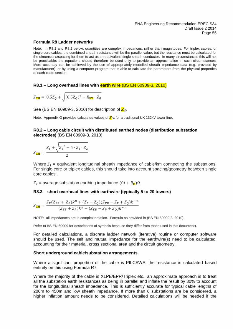
ENA Engineering Recommendation EREC S34 Draft Issue 2 2014
Page 55
Formula R8 Ladder networks
Note: In R8.1 and R8.2 below, quantities are complex impedances, rather than magnitudes. For triplex cables, or single core cables, the combined sheath resistance will be the parallel value, but the reactance must be calculated for the dimensions/spacing for them to act as an equivalent single sheath conductor. In many circumstances this will not be practicable; the equations should therefore be used only to provide an approximation in such circumstances. More accuracy can be achieved by the use of appropriately modelled sheath impedance data (e.g. provided by manufacturer), or by using a computer program that is able to calculate the parameters from the physical properties of each cable section.
R8.1 – Long overhead lines with earth wire (BS EN 60909-3, 2010)
𝑍CH = 0.5𝑍𝑄 + √(0.5𝑍𝑄)2 + 𝑅ET ⋅ 𝑍𝑄
See (BS EN 60909-3, 2010) for description of ZQ.
Note: Appendix G provides calculated values of ZCH for a traditional UK 132kV tower line.
R8.2 – Long cable circuit with distributed earthed nodes (distribution substation electrodes) (BS EN 60909-3, 2010)
𝑍CH = 𝑍1 + √𝑍1
2 + 4 ⋅ 𝑍1 ⋅ 𝑍2
2
Where 𝑍1 = equivalent longitudinal sheath impedance of cable/km connecting the substations. For single core or triplex cables, this should take into account spacing/geometry between single core cables .
𝑍2 = average substation earthing impedance (0𝑗 + 𝑅B)Ω
R8.3 – short overhead lines with earthwire (typically 5 to 20 towers)
𝑍CH = 𝑍𝑃(𝑍𝐸𝐵 + 𝑍𝑃)𝑘𝑛 + (𝑍𝑃 − 𝑍𝑄)(𝑍𝐸𝐵 − 𝑍𝑃 + 𝑍𝑄)𝑘− 𝑛
(𝑍𝐸𝐵 + 𝑍𝑃)𝑘𝑛 − (𝑍𝐸𝐵 − 𝑍𝑃 + 𝑍𝑄)𝑘− 𝑛
NOTE: all impedances are in complex notation. Formula as provided in (BS EN 60909-3, 2010).
Refer to BS EN 60909 for descriptions of symbols because they differ from those used in this document).
For detailed calculations, a discrete ladder network (iterative) routine or computer software should be used. The self and mutual impedance for the earthwire(s) need to be calculated, accounting for their material, cross sectional area and the circuit geometry.
Short underground cable/substation arrangements.
Where a significant proportion of the cable is PILCSWA, the resistance is calculated based entirely on this using Formula R7.
Where the majority of the cable is XLPE/EPR/Triplex etc., an approximate approach is to treat all the substation earth resistances as being in parallel and inflate the result by 30% to account for the longitudinal sheath impedance. This is sufficiently accurate for typical cable lengths of 200m to 450m and low sheath impedance. If more than 6 substations are be considered, a higher inflation amount needs to be considered. Detailed calculations will be needed if the

ENA Engineering Recommendation EREC S34 Draft Issue 2 2014
Page 56
substation earth resistances approach 1 ohm or less, because the sheath impedance then becomes significant. For detailed calculations, a discrete ladder network (iterative) routine or computer software should be used.
See also (BS EN 60909-3, 2010) for more details of the calculations for ladder networks, including non-symmetrical arrangements.
Formula R9 Accounting for proximity effects
The resistance 𝑅𝑡 in ohms (Ω) of n vertically driven rods set s metres apart may be calculated from:
𝑅𝑡 =1
𝑛
𝜌
2𝜋𝐿R[𝑙𝑜𝑔𝑒 (
8𝐿R
𝑑) − 1 +
𝐿R
𝑠]
Where:
𝜌 is the resistivity of soil, in ohm metres (·m);
𝐿R is the length of the electrode, in metres (m);
𝑛 is the number of rods;
𝑠 is the spacing between rods
and
is a group factor where: = 2 (1
2+ ⋯+
1
𝑛)
NOTE: For larger values of n, can be approximated by: ~ 2 𝑙𝑜𝑔𝑒 1.781𝑛
2.818
(Source: Sunde, E.D.: Earth conduction effects in transmission systems, Dover Publications, 1967, pp75-79)
Computer software is best used to account for proximity effects where strip electrodes or PILCSWA type cables run in parallel. An approximation of this effect can be made using proximity factors such as those illustrated in Table B.3 below. Strip electrodes of about 120m in uniform soil are a set distance apart. Each provides a resistance of 2Ω in uniform soil and in the absence of the effect, a parallel resistance of 1Ω would be anticipated. The table shows the higher resistance and proximity factor that applies, clearly increasing when the electrodes are closer together.
Separation distance
(m)
Overall resistance
(Ω)
Proximity factor
1 1.57 1.57
5 1.38 1.38
10 1.3 1.3
20 1.22 1.22
50 1.125 1.125
100 1.07 1.07

ENA Engineering Recommendation EREC S34 Draft Issue 2 2014
Page 57
Table B.3 Proximity effect of electrodes run in parallel (calculated using computer software)
Formula R10 Overall earth resistance
𝑍E = (1
𝑅ES+
1
𝑍CH1+
1
𝑍CH2+ ⋯)
−1
The overall impedance of an earthing system can be approximated to the parallel combination of all
component parts. This formula neglects proximity effects (overlapping resistance areas) and will generally
provide a lower value for 𝑍E than might be observed in practice (or provided by simulation results).
Formula C1 Current rating formula
For fault currents which are interrupted in less than 5s the cross-section of earthing conductor or earth electrode shall be calculated from the following formula D.1 (IEC 60287 - 3-1 Ed 1.1b, 1999)
𝐴 =𝐼
𝐾 √
𝑡𝑓
𝑙𝑜𝑔𝑒 (𝛩𝑓 + 𝛽𝛩𝑖 + 𝛽
)
(Source: IEC 60949, formula D1)
where:
𝐴 is the cross-section in mm2
𝐼 is the conductor current in amperes (RMS value)

ENA Engineering Recommendation EREC S34 Draft Issue 2 2014
Page 58
𝑡𝑓 is the duration of the fault in seconds
𝐾
is a constant depending on the material of the current-carrying component; Table D.1 of IEC 60949 provides values for the most common materials assuming an initial temperature of 20°C
𝛽 is the reciprocal of the temperature coefficient of resistance of the current-carrying component at 0°C (see Table below).
𝛩𝑖
is the initial temperature in degrees Celsius. Values may be taken from (IEC 60287-3-1 Ed. 1.1 b : 1999, Electric cables - Calculation of the current rating - Part 3-1: Sections on operating conditions - Reference operating conditions and selection of cable type, 1999). If no value is laid down in the national tables, 20°C as ambient ground temperature at a depth of 1m should be adopted.
𝛩𝑓 Is the final temperature in degrees Celsius
Note: Care should be taken not to exceed safe temperatures for cable sheaths (and their insulation), particularly on heavily loaded circuits where the initial temperature may be close to 90ºC.
Formula C2 Limit of Surface Current Density formula
Actual current:
Surface Current Density =𝐸𝑙𝑒𝑐𝑡𝑟𝑜𝑑𝑒 𝐶𝑢𝑟𝑟𝑒𝑛𝑡
𝑆𝑢𝑟𝑓𝑎𝑐𝑒 𝐴𝑟𝑒𝑎 𝑜𝑓 𝐸𝑙𝑒𝑐𝑡𝑟𝑜𝑑𝑒
Limiting current:
𝐽𝑙𝑖𝑚𝑖𝑡 = 10−3 (57.7
𝜌𝑡)1/2
where:
𝜌 is the soil resistivity (Ωm)
𝑡 is the fault duration (seconds)

ENA Engineering Recommendation EREC S34 Draft Issue 2 2014
Page 59
6.7 Surface potential formulae (P)
For substations with separately earthed fence and normal buried grid depths (typically 0.6 m):
Formula P1 External touch potential at the edge of the electrode
𝑈T =𝑘𝑒 ∙ 𝑘𝑑 ∙ 𝜌 ∙ 𝐼𝐸
𝐿T
(V)
where
𝑘𝑒 =1
𝜋(1
2𝑙𝑜𝑔𝑒
ℎ
𝑑+
1
2ℎ+
1
(0.5 + D)+
1
D(1 − 0.5𝑛−2))
𝑘𝑒 is a factor that allows for the effect of a uniformly distributed electrode current over the grid and is given by:
ℎ = grid depth (m)
𝑑 = equivalent diameter of conductor = circumference of conductor
π (m)
𝜌 = soil resistivity ( m)
𝐼𝐸 = total current passing to ground through electrode (A)
D = average spacing between parallel grid conductors (m)
𝑛 = (𝑛𝐴 × 𝑛𝐵)1
2⁄
where 𝑛𝐴 = number of parallel grid conductors in one direction
where 𝑛𝐵 = number of parallel grid conductors in the other direction
𝑘𝑑 is a factor, which modifies 𝑘𝑒 to allow for the non-uniform distribution of electrode current, and is given by:
𝑘𝑑 = (0.7 + 0.3𝐿T
𝐿p)
kd = (0.7 + 0.3L
Lp)ke =
1
π(
1
2loge
h
d+
1
2h+
1
(0.5+D)+
1
D(1-0.5n-2))
where
𝐿T = total length of buried electrode conductor including rods if connected (m)
𝐿p = perimeter length of buried electrode conductor including rods if connected (m)
𝐼𝐸 = total current passing to ground through electrode (A)
𝑈T = resulting touch potential or, when assessing length 𝐿, the safe touch potential
from Figure 2

ENA Engineering Recommendation EREC S34 Draft Issue 2 2014
Page 60
Formula P2 External ‘Touch’ potential at the fence
The ground current density is significantly diminished at the fence compared to that at the edge of the grid electrode. As a result, a new factor, 𝑘𝑓, based on a two-metre separation between
fence and grid electrode, is applied in place of 𝑘𝑒 in the above formulae.
Hence:
UvT(fence) =𝑘𝑓 ∙ 𝑘𝑑 ∙ 𝜌 ∙ 𝐼𝐸𝑆
𝐿𝑃
(𝑉) 𝑜𝑟 𝐿𝑃 =𝑘𝑓 ∙ 𝑘𝑑 ∙ 𝜌 ∙ 𝐼𝐸𝑆
𝐸𝑡𝑜𝑢𝑐ℎ(𝑚)
where 𝑘𝑓 = 0.26𝑘𝑒
Substation with integrally earthed fence
There are two situations to be considered. The first is where the fence is situated at the edge of the substation electrode. The second has a peripheral electrode conductor buried half a metre below the surface, one metre beyond the fence and regularly bonded to it.
External touch potential at fence with no external peripheral electrode
𝐸T(𝑓𝑒𝑛𝑐𝑒) is the same as 𝐸T(𝑔𝑟𝑖𝑑) using P1 as above.
Formula P3 External touch potential at fence with external buried peripheral
conductor 1m from fence
UvT(fence) =𝑘𝑓𝑒 ∙ 𝑘𝑑 ∙ 𝜌 ∙ 𝐼𝐸𝑆
𝐿𝑃
(𝑉) 𝑜𝑟 𝐿𝑃 =𝑘𝑓𝑒 ∙ 𝑘𝑑 ∙ 𝜌 ∙ 𝐼𝐸𝑆
𝐸𝑡𝑜𝑢𝑐ℎ(𝑚)
Where 𝑘𝑓𝑒 = (1
2𝑙𝑜𝑔𝑒
ℎ
𝑑−
1
4𝑙𝑜𝑔𝑒(𝑆
2 + 0.52)2 +1
4𝑙𝑜𝑔𝑒(𝑆
4 + 𝑆2))
ℎ and 𝑑 are as in formula P1
𝑆 = distance between the outermost buried grid conductor and the next nearest parallel conductor (m)

ENA Engineering Recommendation EREC S34 Draft Issue 2 2014
Page 61
Formula P4 Touch voltage within grid (from IEEE80)
The touch voltage within the earth grid may be calculated using the following equations from
IEEE-80, Annex D and is defined as the Mesh Voltage. It is the touch voltage that would be
experienced at the center of a corner mesh in an earth grid with an equally spaced mesh.
Note: Terms used in these equations are not ‘globally’ defined in the rest of this document, and are included here for consistency with the source document (IEEE 80).
𝐸𝑚 =𝜌 × 𝐼𝐸𝑆 × 𝐾𝑚 × 𝐾𝑖
𝐿𝐶 +
[ 1.55 + 1.22 ×
(
𝐿𝑟
√𝐿𝑥2 + 𝐿𝑦
2
)
] × 𝐿𝑅
𝐾𝑚 =1
2 × 𝜋× [𝑙𝑛 [
𝐷2
16 × ℎ × 𝑑+
(𝐷 + 2 × ℎ)2
8 × 𝐷 × 𝑑−
ℎ
4 × 𝑑] +
𝐾𝑖𝑖
𝐾ℎ× 𝑙𝑛 [
8
𝜋(2 × 𝑛 − 1)]]
𝐾𝑖 = 0.644 + 0.148 × 𝑛
𝑛 = 𝑛𝑎 × 𝑛𝑏 × 𝑛𝑐 × 𝑛𝑑
𝑛𝑎 =2 × 𝐿𝐶
𝐿𝑝
𝑛𝑏 = 1 𝑓𝑜𝑟 𝑠𝑞𝑢𝑎𝑟𝑒 𝑔𝑟𝑖𝑑𝑠, 𝑜𝑡ℎ𝑒𝑟𝑤𝑖𝑠𝑒: 𝑛𝑏 = √𝐿𝑝
4 × √𝐴
𝑛𝑐 = 1 𝑓𝑜𝑟 𝑠𝑞𝑢𝑎𝑟𝑒 𝑎𝑛𝑑 𝑟𝑒𝑐𝑡𝑎𝑛𝑔𝑢𝑙𝑎𝑟 𝑔𝑟𝑖𝑑𝑠, 𝑜𝑡ℎ𝑒𝑟𝑤𝑖𝑠𝑒: 𝑛𝑐 = [𝐿𝑥 × 𝐿𝑦
𝐴]
0.7×𝐴𝐿𝑥×𝐿𝑦
𝑛𝑑 = 1 𝑓𝑜𝑟 𝑠𝑞𝑢𝑎𝑟𝑒, 𝑟𝑒𝑐𝑡𝑎𝑛𝑔𝑢𝑙𝑎𝑟 𝑎𝑛𝑑 𝐿 − 𝑠ℎ𝑎𝑝𝑒𝑑 𝑔𝑟𝑖𝑑𝑠, 𝑜𝑡ℎ𝑒𝑟𝑤𝑖𝑠𝑒: 𝑛𝑑 =𝐷𝑚
√𝐿𝑥2 + 𝐿𝑦
2
𝐾ℎ = √1 +ℎ
ℎ0
𝐾𝑖𝑖 = 1
for grids with numerous earth rods, especially where they are located at the corners and around
the perimeter
𝐾𝑖𝑖 =1
(2×𝑛)2𝑛

ENA Engineering Recommendation EREC S34 Draft Issue 2 2014
Page 62
for grids with no (or very few) earth rods, especially where they are not located on corners or
around the perimeter.
Where:
Em is the mesh voltage (V)
ρ is the average soil resistivity (Ωm)
IES is the electrode current (A)
LC is the total length of horizontal conductor in the grid (m)
LR is the total length of all earth rods (m)
Lr is the average earth rod length (m)
Lp is the length of the perimeter conductor (m)
Lx is the maximum length of the grid in the x direction (m)
Ly is the maximum length of the grid in the y direction (m)
D is the spacing between parallel conductors in the mesh (m)
d is the diameter of the earth conductors (m)
h is the grid burial depth (m)
A is the area of the grid (m2)
Dm is the maximum distance between any two points on the grid (m)
h0 is the grid reference depth of 1m
Formula P5 Step voltage on outside edge of grid
UvS =𝜌𝐼F2𝜋𝑟
(𝑎𝑟𝑐𝑠𝑖𝑛𝑟
𝑥− 𝑎𝑟𝑐𝑠𝑖𝑛
𝑟 + 1
𝑥) where 𝑟 =
𝜌
4𝑅E
X = distance from (centre of?) grid.
Formula P6 Voltage profile around earth electrode
COLUMN P6.1 P6.2 P6.3

ENA Engineering Recommendation EREC S34 Draft Issue 2 2014
Page 63
ELECTRODE DESCRIPTION
HEMISPHERE VERTICAL ROD BURIED GRID
CONFIGURATION
VOLTAGE ON THE SURFACE
OF THE GROUND AT POINT ‘S’
WITH RESPECT TO TRUE EARTH
𝑉S =𝜌𝐼
2𝜋𝑥
𝑉S =
𝜌𝐼
2𝜋ℓlog𝑒 (
ℓ
𝑥+ √1 +
ℓ2
𝑥2)
𝑉S =𝜌𝐼
2𝜋ℓarc sin
𝑟
𝑥
where:
𝑟 =𝜌
4𝑅𝐸 and
arc sin𝑟
𝑥 is in radians

ENA Engineering Recommendation EREC S34 Draft Issue 2 2014
Page 64
Formula P7 Calculation of specific external potential contours
𝑥 = √𝐴
𝜋[(𝑠𝑖𝑛
𝑉𝑥 𝜋
2𝑈E)−1
− 1]
Note: Angles are in radians
where 𝑥 is the distance in metres to a point where the surface potential is 𝑉𝑥 volts.
𝐴 = superficial area of grid electrode in square metres.
𝑈E = earth potential rise in volts.
These formulae apply on the basis that the earthing installation may be treated as equivalent to a symmetrical grid.
Substation fences are usually earthed independently from the main earthing system and may be up to 2m from it. By using the above formulae as the “high EPR zone” radii, a factor of safety is introduced when they are measured from the substation fence. Some discretion may be necessary in assessing the “hot zone” radius of a substation where the fence is bonded to the earthing installation or there is a large distance from the fence to the edge of the earthing system.
Clearly this formula does not apply when 𝑈E is lower than the voltage contour of interest.
Installation Complete
Obtain Basic Data (ENA TS 41-24 Ch8):
• Substation Plan• Earth Fault Currents (S34 Ch..)• Fault Duration
Select Earth Conductor Sizes(ENA TS 41-24 Ch8)
Use Standard Design or Apply Standard Design Methodology to Meet
Functional Requirements(ENA TS 41-24 Ch7)
Existing Site orNew One Connected to Existing Infrastructure?
Assess and Measure Existing Earthing
(ENA TS 41-24 Ch12, Ch13)
Is the Site in an
Urban Location?
Carry Out Soil Resistivity Measurements
(ENA TS 41-24 Ch12) and/or Obtain Soil Data
Produce Soil Model
Cable Fed and Fault Current less
than 1000A?
Install Standard Design or Use Standard Methodology
(ENA TS 41-24 Ch7)
Design Electrode System Based Upon Standard Methodology (ENA TS 41-24 Ch7)
Use Soil and Electrode Parameters to Estimate Resistance Values With Parallel Paths
(S34 Ch..)
Carry Out Fault Current Analysis and Distribution Study
(S34 Ch..)
Obtain Ground Return Current(S34 Ch..)
Calculate EPR (S34 Ch..)and obtain Safety Limit Values (ENA TS 41-24 Ch6)
Is EPR < 2x Touch Voltage Limit?
Is EPR < 4x Touch Voltage Limit?
Calculate Touch Voltages(S34 Ch..)
Implement Specific Measures (See ENA-TS 41-24 Ch..) Is V
T < Touch
Voltage Limit?
Finalise/Approve DetailedDesign for Installation
Carry Out Commissioning Measurements(ENA TS 41-24 Ch12)
Do Measurements Agree Reasonably With Design?
Carry Out Risk AssessmentBS EN50522 NANB(ENA TS 41-24 Ch..)
Does Risk ExceedALARP Level?
Modify Design
Review Design Calculations
Are Differences Significant?
Install SystemENA TS 41-24 Ch10
DESIGN PROCESS(ENA TS 41-24 Ch9)
Y
Y
Y
Y
Y
Y
Y
Y
Y
N
N
N
N
N
N
N
N
N

ENA Engineering Recommendation EREC S34 Draft Issue 2 2014
Page 65
APPENDIX C – Earthing design methodology
COPY FINAL VERSION FROM 41-24 when complete
[TO DO – but not yet, as includes references to 41-24 chapters so make sure 41-24 is finalised]
Installation Complete
Obtain Basic Data (ENA TS 41-24 Ch8):
• Substation Plan• Earth Fault Currents (S34 Ch..)• Fault Duration
Select Earth Conductor Sizes(ENA TS 41-24 Ch8)
Use Standard Design or Apply Standard Design Methodology to Meet
Functional Requirements(ENA TS 41-24 Ch7)
Existing Site orNew One Connected to Existing Infrastructure?
Assess and Measure Existing Earthing
(ENA TS 41-24 Ch12, Ch13)
Is the Site in an
Urban Location?
Carry Out Soil Resistivity Measurements
(ENA TS 41-24 Ch12) and/or Obtain Soil Data
Produce Soil Model
Cable Fed and Fault Current less
than 1000A?
Install Standard Design or Use Standard Methodology
(ENA TS 41-24 Ch7)
Design Electrode System Based Upon Standard Methodology (ENA TS 41-24 Ch7)
Use Soil and Electrode Parameters to Estimate Resistance Values With Parallel Paths
(S34 Ch..)
Carry Out Fault Current Analysis and Distribution Study
(S34 Ch..)
Obtain Ground Return Current(S34 Ch..)
Calculate EPR (S34 Ch..)and obtain Safety Limit Values (ENA TS 41-24 Ch6)
Is EPR < 2x Touch Voltage Limit?
Is EPR < 4x Touch Voltage Limit?
Calculate Touch Voltages(S34 Ch..)
Implement Specific Measures (See ENA-TS 41-24 Ch..) Is V
T < Touch
Voltage Limit?
Finalise/Approve DetailedDesign for Installation
Carry Out Commissioning Measurements(ENA TS 41-24 Ch12)
Do Measurements Agree Reasonably With Design?
Carry Out Risk AssessmentBS EN50522 NANB(ENA TS 41-24 Ch..)
Does Risk ExceedALARP Level?
Modify Design
Review Design Calculations
Are Differences Significant?
Install SystemENA TS 41-24 Ch10
DESIGN PROCESS(ENA TS 41-24 Ch9)
Y
Y
Y
Y
Y
Y
Y
Y
Y
N
N
N
N
N
N
N
N
N

ENA Engineering Recommendation EREC S34 Draft Issue 2 2014
Page 66
APPENDIX D – Formulae for determination of ground return current for earth faults on metal sheathed cables
The current in the core of a single-core cable or the unbalance of current in the cores of a multicore cable induces a voltage in the metallic sheath/armour of the cable. If the sheath/armour is connected to earth at each end of its length, a current will be driven through the sheath/armour earth loop which constitutes part of the earth fault current returning from the fault, the remainder being that returning in the ground. The quantity of current returning in the cable sheath/armour is, inter alia, dependent on the location of the cable in the system with respect to the source of fault current infeed and to the position of the fault as well as on the values of the sheath/armour terminating earth resistances.
Formulae for the computation of the ground current are given below, in respect of a cable terminated and earthed at points A and B.
The arrangements considered are illustrated in Figures D.1 to D.4.
Figure D.1 Cable, Local Source of Fault at Cable End.
Figure D.2 Line-Cable-Line, Remote Source and Remote Fault
AC
LC km
RA RB
IF
IE
IS
LC km
RA RB
IF
IE
AC
IS
IF IF

ENA Engineering Recommendation EREC S34 Draft Issue 2 2014
Page 67
Figure D.3 Cable-Line, Local Source and Remote Fault
Figure 0-2 - Line-Cable, Remote Source and Fault at Cable End
1a. Three-core cable (unarmoured), source of infeed at point A and fault at point B. See diagram Figure D.1.
𝐼ES = −𝐼F [𝑙(𝑧𝑐 − 𝑧𝑚𝑝,𝑐)
𝑙𝑧𝑐 + 𝑅A + 𝑅B] = −𝐼F [
𝑙𝑟𝑐𝑙𝑧𝑐 + 𝑅A + 𝑅B
]
1b. Three-core cable (armoured), source of infeed at point A and fault at point B. See Figure D.1.
RB
AC
LC km
RA
IF
IE
IS
IF
AC
LC km
RA RB
IF
IE
IS
IF

ENA Engineering Recommendation EREC S34 Draft Issue 2 2014
Page 68
𝐼ES = −𝐼F
[ 𝑙 (
𝑟𝑐 × 𝑟𝑎𝑟𝑐 + 𝑟𝑎
)
𝑙 ((𝑟𝑐 × 𝑟𝑎𝑟𝑐 + 𝑟𝑎
) + 𝑟𝑒 + 𝑗𝜔(𝐿𝑐 + 𝐿𝑎)) + 𝑅A + 𝑅B
]
2a. Three-core cable (unarmoured), source of infeed beyond point A and fault beyond point B. See Figure D.2.
𝐼ES = −𝐼F [𝑙(𝑧𝑐 − 𝑧𝑚𝑝,𝑐) + 𝑅A + 𝑅B
𝑙𝑧𝑐 + 𝑅A + 𝑅B] = −𝐼F [
𝑙𝑟𝑐 + 𝑅A + 𝑅B
𝑙𝑧𝑐 + 𝑅A + 𝑅B]
2b. Three-core cable (armoured), source of infeed beyond point A and fault beyond point B. See Figure D.2.
𝐼ES = −𝐼F
[ 𝑙 (
𝑟𝑐 × 𝑟𝑎𝑟𝑐 + 𝑟𝑎
)𝑅A + 𝑅B
𝑙 ((𝑟𝑐 × 𝑟𝑎𝑟𝑐 + 𝑟𝑎
) + 𝑟𝑒 + 𝑗𝜔(𝐿𝑐 + 𝐿𝑎)) + 𝑅A + 𝑅B]

ENA Engineering Recommendation EREC S34 Draft Issue 2 2014
Page 69
3a. Three-core cable (unarmoured), source of infeed beyond point A and fault at point B, or source of infeed at point B and fault beyond point A. See Figures D.3 and D.4.
𝐼ES = −𝐼F [𝑙(𝑧𝑐 − 𝑧𝑚𝑝,𝑐) + 𝑅A
𝑙𝑧𝑐 + 𝑅A + 𝑅B] = −𝐼F [
𝑙𝑟𝑐 + 𝑅A
𝑙𝑧𝑐 + 𝑅A + 𝑅B]
3b. Three-core cable (armoured), source of infeed at point A and fault at point B, or source of infeed at point B and fault beyond point A. See Figures 11 and 13.
𝐼ES = −𝐼F
[ 𝑙 (
𝑟𝑐 × 𝑟𝑎𝑟𝑐 + 𝑟𝑎
)𝑅A
𝑙 ((𝑟𝑐 × 𝑟𝑎𝑟𝑐 + 𝑟𝑎
) + 𝑟𝑒 + 𝑗𝜔(𝐿𝑐 + 𝐿𝑎)) + 𝑅A]
4. Three single-core cables, source of infeed at point A and fault at point B; the cable sheaths are referenced 1, 2, 3. See diagram Fig. 14, Evaluate sheath currents I1, I2 and I3 and determine IES from the following:
[
(𝑅A + 𝑙𝑧𝑐1 + 𝑅B) (𝑅A + 𝑙𝑧𝑚1,2 + 𝑅B) (𝑅A + 𝑙𝑧𝑚1,3 + 𝑅B)
(𝑅A + 𝑙𝑧𝑚1,2 + 𝑅B) (𝑅A + 𝑙𝑧𝑐2 + 𝑅B) (𝑅A + 𝑙𝑧𝑚2,3 + 𝑅B)
(𝑅A + 𝑙𝑧𝑚1,3 + 𝑅B) (𝑅A + 𝑙𝑧𝑚2,3 + 𝑅B) (𝑅A + 𝑙𝑧𝑐3 + 𝑅B)
] [𝐼1𝐼2𝐼3
] = −𝐼F [
(𝑅A + 𝑙𝑧𝑚𝑝,1 + 𝑅B)
(𝑅A + 𝑙𝑧𝑚𝑝,2 + 𝑅B)
(𝑅𝐴 + 𝑙𝑧𝑚𝑝,3 + 𝑅𝐵)
]
𝐼𝐸𝑆 = −𝐼𝐹 − 𝐼1 − 𝐼2 − 𝐼3
5. Three single-core cables, source of infeed beyond point A and fault beyond point B. See diagram Fig. 15.
Evaluate sheath currents I1, I2 and I3 and determine IES from the following:
[IMPEDANCE COEFFICIENTS
AS IN (4) ABOVE] [
𝐼1𝐼2𝐼3
] = −𝐼F [
(𝑙𝑧𝑚𝑝,1)
(𝑙𝑧𝑚𝑝,2)
(𝑧𝑚𝑝,3)
]
𝐼𝐸𝑆 = −𝐼𝐹 − 𝐼1 − 𝐼2 − 𝐼3
6. Three single-core cables, source of infeed beyond point A and fault at point B, or source of infeed at point B and fault beyond point A. See diagrams Figs. 16 and 17.
Evaluate sheath currents I1, I2 and I3 and determine IES from the following:
[IMPEDANCE COEFFICIENTS
AS IN (4) ABOVE] [
𝐼1𝐼2𝐼3
] = −𝐼F [
(𝑙𝑧𝑚𝑝,1 + 𝑅B)
(𝑙𝑧𝑚𝑝,2 + 𝑅B)
(𝑧𝑚𝑝,3 + 𝑅B)
]
𝐼𝐸𝑆 = −𝐼𝐹 − 𝐼1 − 𝐼2 − 𝐼3
The parameters used in the above formulae are as given in the list of symbols shown in Section 3.1 or as defined below.
The quantities 𝑧𝑐 ; 𝑧𝑐1 ; 𝑧𝑐2 ; 𝑧𝑐3 are the sheath to earth self impedances at 50 Hz.

ENA Engineering Recommendation EREC S34 Draft Issue 2 2014
Page 70
𝑍𝐶 = 𝑟𝑐 + (49.4 + 𝑗62.8 𝑙𝑜𝑔𝑒
93.2√𝜌
𝑐𝑔) ×
10−3𝛺
𝑘𝑚 (Ω/𝑘𝑚)
where 𝑐𝑔 is the GMR (Geometric Mean Radius) of the sheath in metres.
The quantity RE is the resistive component of the ground return path of the sheath to earth self impedance.
= 5𝜋210−3Ω/km – EDIFERA to sanity check using CDEGS
= (0.2 𝑙𝑜𝑔𝑒
93.2√𝜌
𝑐𝑔) × 10−3𝛺/𝑘𝑚
The quantity 𝐿𝑐 is the inductive component of the sheath to earth self impedance.
The quantity 𝐿𝑎 is the effective inductance of the armour wire.
𝐿𝑎 = (0.4𝜇𝑡
𝑑𝑖 + 𝑡) × 10−3 (𝐻/𝑘𝑚)
Where 𝑡 is the thickness of the armour wire in metres.
𝑑𝑖 is the internal diameter of the armour wire in metres.
𝜇 is the relative permeability of the armour material The quantities 𝑧𝑚𝑝,𝑐; 𝑧𝑚𝑝,1; 𝑧𝑚𝑝,2 and 𝑧𝑚𝑝,3 are the faulty conductor to sheath mutual impedances
and 𝑧𝑚1,2; 𝑧𝑚1,3 and 𝑧𝑚2,3 are the sheath-to-sheath mutual impedances at 50 Hz.
𝑍𝑚𝑝,𝐶 = (49.4 + 𝑗62.8 𝑙𝑜𝑔𝑒93.2√𝜌
𝑑) × 10−3 /km
where d is the centre to centre distance in metres between the conductors/sheaths.
In calculating 𝑧𝑚𝑝,𝑐; 𝑧𝑚𝑝,1; 𝑧𝑚𝑝,2 and 𝑧𝑚𝑝,3 the value of d has been substituted for 𝑐𝑔 (where 𝑐𝑔 is
the GMR of the sheath in metres).
In the following table, the values of 𝑧𝑐 and 𝑧𝑚𝑝,𝑐 for three-core cables in common use are listed for
an assumed value of ρ of 100 m.

ENA Engineering Recommendation EREC S34 Draft Issue 2 2014
Page 71
System
Voltage
Cable Type
(3-core/triplex)
Impedances in /km
with 35mm
2
screens zc zmp,c zc zmp,c zc zmp,c
11 kV
Conductor CSA 0.1 in2 185 mm
2 300 mm
2
PILC
SWA
1.221
33.24
0.672
85.8
1.099
41.6
0.674
85.8
0.873
49.1
0.622
85.8
PILC 1.228
33.77
0.686
85.88
0.999
41.66
0.667
85.77
0.858
49.53
0.656
85.69
PICAS 0.677
77.33
0.662
85.6
0.658
79.6
0.649
85.7
TRIPLEX 0.89
51.8
0.703
86
0.875
52
0.691
85.92
33 kV
Conductor CSA 0.2 in
2
185 mm2
300 mm2
PILC
SWA
0.753
58.62
0.646
85.62
0.769
56.4
0.651
85.7
0.735
60.3
0.641
85.6
PILC 0.753
58.63
0.646
85.63
0.771
56.35
0.644
85.62
PICAS 0.684
74
0.659
85.7
0.667
76.3
0.65
85.7
TRIPLEX 0.87
51.8
0.683
85.87
0.856
51.5
0.672
85.8
132 kV
Conductor CSA 185 mm2 300 mm
2
PILC
SWA
0.652
76
0.635
85.6
0.645
76.7
0.63
85.5
TRIPLEX*
(135mm2
Cu screen)
0.63
80.71
0.625
85.48
0.67
74.78
0.649
85.65
PICAS 0.636
79.6
0.628
85.5
0.63
80.2
0.623
85.5
PILC 0.771
56.35
0.644
85.62
0.725
60.98
0.637
85.57
Table D.1 Self and mutual impedances for a sample of distribution cables
NOTE 1: In all cases the phase angle is negative

ENA Engineering Recommendation EREC S34 Draft Issue 2 2014
Page 72
*NOTE 2: For triplex cables and single core cables, the table above gives single core values. These may be used directly in formulas XXX to provide an approximate calculation of ground return current (IES). The three core equivalent cable data may be used if available. In either case this neglects the mutual coupling between each core and neighbouring cores/sheaths and is slightly less accurate than the use of formula XXX with appropriate Zm1,2(etc.) values
NOTE 3: PILCSWA = paper insulated lead sheath covered steel wire armour; PILC= paper insulated lead sheath covered; PICAS= Paper insulated corrugated aluminium sheathed; TRIPLEX= 3 x single core cables with XLPE or EPR insulation and 35mm
2 stranded copper screen/cable (11kV and 33kV) or 135mm
2 screen (132kV).

ENA Engineering Recommendation EREC S34 Draft Issue 2 2014
Page 73
APPENDIX E – Ground current for earth faults on steel tower supported circuits with an aerial earthwire
Values of ground current IE as a percentage of IF and corresponding phase angle ØE with respect to IF for 132 kV, 275 kV and 400 kV line constructions
Type of Line and Conductor Size (mm2)
IE as a percentage of IF Phase Angle of IE with
respect to IF (ØE degrees lead)
132 kV (L4)
(1 × 175) 70.8 171
132 kV (L7)
(2 × 175) 63.6 177
275 kV (L3)
(2 × 175) 66.9 178
275 kV (L2)
(2 × 400) 68.6 178
400 kV (L8)
(2 × 400) 70.0 179
400 kV (L6)
(4 × 400) 69.2 179
400 kV (L9)
(4 × 400) 64.0 179

ENA Engineering Recommendation EREC S34 Draft Issue 2 2014
Page 74
APPENDIX F – Chart to calculate resistance of horizontal electrode

ENA Engineering Recommendation EREC S34 Draft Issue 2 2014
Page 75

ENA Engineering Recommendation EREC S34 Draft Issue 2 2014
Page 76
APPENDIX G – Chain impedance of standard 132kV earthed tower lines
The table below provides chain impedances for a 132kV L4 type construction with three towers/km and a horse earth wire (approx 70mm2 aluminium ACSR, to BS 215 pt5 1970).
Longitudinal impedance of earth wire is 0.443 + j 0.757 ohm/km (calculated using Carson Clem formula).
The values assume more than 20 towers in series.
Footing resistance (ohm)
Chain impedance r + j x ohm
Chain impedance
ZCH ohm
1 0.543+j0.414 0.68337.35
2 0.737+j0.52 0.90235.21
3 0.886+j0.603 1.07234.24
4 1.012+j0.674 1.21533.7
5 1.122+j0.736 1.34233.26
6 1.222+j0.793 1.45732.96
7 1.314+j0.845 1.56232.73
8 1.4+j0.893 1.66132.55
9 1.48+j0.939 1.75332.39
10 1.556+j0.982 1.84132.26
15 1.89+j1.172 2.22431.82
20 2.17+j1.333 2.54731.55
25 2.42+j1.474 2.83231.37
40 3.039+j1.83 3.54731.05

ENA Engineering Recommendation EREC S34 Draft Issue 2 2014
Page 77
APPENDIX H – Sample calculations showing the effect on the ground return current for change in the separation distance between three single core cables laid flat or in trefoil
For the studies described below, three representative cables were selected for 11kV and
132kV voltage levels. Their details are given in Table H.1.
Note: The values provided in this section are for comparison purposes only, to illustrate the effect of cable laying only. R1 and R2 may be assumed nominal values.
Operating voltage
(kV)
Cable
number
Phase conductor size
mm2
Insulation type
Insulation thickness
mm
Core / Screen type + size mm
2
Reference cable code
132 1 630 XLPE 15 Lead 132_01_12
132 2 630 XLPE 21 Lead 132_01_13
132 3 630 XLPE 15 Copper wire
135 132_01_17
11 4 70 EPR Copper wire 12 11_3_SZ
11 5 300 EPR Copper wire 35 11_225_EPR
11 6 300 XLPE Copper wire 70 11_21_S
Table H.1 Technical details of cables modelled
The geometric arrangements considered are trefoil and flat. They are analysed on the basis that they are installed such that the cables are touching and again assuming they are a symmetrical distance 3 x D apart (where D is the outer cable diameter in mm). See Table H.2 for details.
TREFOIL FLAT
Adjacent

ENA Engineering Recommendation EREC S34 Draft Issue 2 2014
Page 78
Distance with 3xD
Table H.2 The geometric placement of cables
3xD
3xD
3xD3xD 3xD

ENA Engineering Recommendation EREC S34 Draft Issue 2 2014
Page 79
IF
IEG
The 132kV cables were selected to show the difference that the sheath/screen configuration makes for the same size phase conductor. One standard cable contains a tubular conductor made of aluminum foil in addition to its stranded copper conductor. The cross-sectional view for this cable (trefoil format) is shown in Figure H.1.
Figure H.1 Cross-sectional view for Cable 3
The circuit used to simulate the different cable arrangements and determine the effect on the earth return current is shown in Figure H.2.
Figure H.2 Circuit used for analysis purposes
Using the circuit described, studies were carried out for each of the cables of Table H.1, and the ground return current calculated for a set range of cable lengths. For each cable, four sets of studies were carried out, i.e. one for each physical arrangement of the individual cables.
The results are shown in Figures H.3 and H.4, with the ground return current 𝐼ES shown as a
percentage of the total earth fault current IF.
1
6
1
6
Zline-1PH
ASE
REP
RES
AN
TATI
ON
OF
THE
SUP
PLY
NET
WO
RK
R1 R2

ENA Engineering Recommendation EREC S34 Draft Issue 2 2014
Page 80
Cable 1: 630mm2 with 15mm XLPE, lead sheathed
Cable 2: 630mm2 with 21mm XLPE, lead sheathed
Cable 3: 630mm2 with 15mm XLPE and composite screen/sheath
(135mm2Cu and 45mm2 Al)
26
30
34
38
42
46
50
54
58
0 2 4 6 8 10 12
I ES/
I F (
%)
Cable Length (km)
10
12
14
16
18
20
22
24
26
0 2 4 6 8 10 12
I ES/
I F (
%)
Cable Length (km)
2
4
6
8
10
12
14
16
0 2 4 6 8 10 12
I ES/
I F (
%)
Cable Length (km) FLAT (3xD) TREFOIL (3xD) FLAT (Adjacent) TREFOIL (Adjacent)

ENA Engineering Recommendation EREC S34 Draft Issue 2 2014
Page 81
Figure H.3 Ground return current (IES) as a percentage of (IF) against circuit length for different 132kV cable installation arrangements

ENA Engineering Recommendation EREC S34 Draft Issue 2 2014
Page 82
Cable 4: (70mm2 with 12mm2 Cu screen)
Cable 5: (300mm2 with 35mm2 Cu screen)
Cable 6: (300mm2 with 70mm2 Cu screen)
6
7
8
9
10
11
12
13
14
15
0 2 4 6 8 10 12
I ES/
IF (%
)
Cable Length (km)
6
7
8
9
10
11
12
13
14
15
0 2 4 6 8 10 12
I ES/
I F (
%)
Cable Length (km)
0
1
2
3
4
5
6
7
0 2 4 6 8 10 12
I ES/
I F (
%)
Cable Length (km) FLAT (3xD) TREFOIL (3xD) FLAT (Adjacent) TREFOIL (Adjacent)

ENA Engineering Recommendation EREC S34 Draft Issue 2 2014
Page 83
Figure H.4 Ground return current (IES) as a percentage of (IF) against circuit length for different 11kV cable installation arrangements
The results show that earth return current increases when the distance between adjacent
cables is increased. The percentage increase in 𝐼ES compared to the touching trefoil arrangement is shown in tables A8.3 and A8.4. The difference is seen to increase with circuit length and cable separation distance.
Cable 1 Cable 2 Cable 3
Circuit length 1 km 10 km 1 km 10 km 1 km 10 km
Difference trefoil (3xD) - trefoil (%) 1.7 7.0 1.6 7.1 1.8 7.5
Difference flat - trefoil (%) 1.3 2.4 1.3 2.4 5.5 6.7
Difference flat (3xD) - trefoil (%) 4.2 11.0 4.2 11.1 9.5 17.1
Table H.3 Effect of physical cable arrangement on ground return current IES for 132 kV cables
Cable 4 Cable 5 Cable 6
Circuit length 1 km 10 km 1 km 10 km 1 km 10 km
Difference trefoil (3xD) - trefoil (%) 1.1 3.6 1.5 6.0 1.7 6.7
Difference flat - trefoil (%) 0.2 0.7 0.6 1.5 1.4 2.4
Difference flat (3xD) - trefoil (%) 1.4 4.5 2.6 8.1 4.4 10.6
Table H.4 Effect of physical cable arrangement on ground return current IES for 11kV cables
Conclusions:
From figures H.3 and H.4, the following can be deduced:-
Touching trefoil is the most effective arrangement in terms of minimising the ground return current. This is as expected, due to the more symmetrical arrangement and its impact on maximising mutual coupling effects. The ground return current increases in all cases in the order touching trefoil, touching flat, 3 x D trefoil and 3 x D flat.
The difference between trefoil and flat arrangements is less than 0.5% of the total and can be disregarded for most studies.
Increasing the separation between the individual cables generally increases the ground return current by less than 1% of the total.
The decrease in cable core insulation thickness from 21mm (in older cables) to 15mm does reduce the ground return current, but by an insignificant amount in relation to other factors (such as measurement errors) and can be ignored for the majority of cases.

ENA Engineering Recommendation EREC S34 Draft Issue 2 2014
Page 84
The two dominant factors influencing the ground return current in these studies are the circuit length and the electrical conductivity of the sheath/screen. The latter is most visibly seen when comparing the 132kV composite screen (copper and aluminium) against a similar cable with a lead screen. The ground return current is more than doubled for the latter. The same effect is apparent with the 11kV cables and cable 4 with its relatively small screen of 12mm2/cable shows the importance of considering the screen size because the ground return current can reach almost 54% for this cable.
Tables H.3 and H.4 are included for completeness and show the increase in the actual ground return current with changes in physical arrangement, as a percentage of the ground return current for the touching trefoil arrangement.
APPENDIX I – Transfer potential to distributed LV systems
I.1 Background
This issue relates to the transfer of voltage from HV systems to LV systems, when the
LV system consists of multiple electrodes, as described in Section 5.4.
I.2 Examples
(a) Equal LV Electrode Earth Resistances
It is useful to consider a worked example where assumed typical values have been used and the transfer voltage has been calculated. Figure I.1 shows the circuit together with the calculated parameters.
Figure I.1 Example – Two Electrodes of Equal Resistance
From Figure I.1, the surface potential experienced by electrodes A and B effectively act as voltage sources. Because electrodes A and B are connected together via an above ground conductor (assumed to have negligible resistance compared to the earth resistances) the potential difference of 100V across the total series resistance of 20Ω causes a current of 5A to
5A
50V 50V
LV Electrode
A
VT = 150V
VB = 100V VA = 200V
RB = 10Ω RA = 10Ω
LV Electrode
B

ENA Engineering Recommendation EREC S34 Draft Issue 2 2014
Page 85
circulate through the electrodes. This creates a voltage drop of 50V across the earth resistance of A which is negative with respect to the local surface potential. This reduces the local electrode potential (by 50V with respect to the local soil potential). Conversely at electrode B there is a 50V potential drop across the earth resistance which increases the electrode potential by 50V with respect to the local soil potential. The transfer potential on the combined LV electrode system is 150V.
This is consistent with the previous work and explains the changes in surface potential contours around combined LV electrodes.

ENA Engineering Recommendation EREC S34 Draft Issue 2 2014
Page 86
(b) Unequal LV Electrode Earth Resistances
Figure I.2 shows a similar example but where Electrode B has an earth resistance 5 times lower than Electrode A.
Figure I.2 Example - Two Electrodes of Unequal Resistance
It can be seen that the potential on the combined LV electrode is much lower than the average value of 150V. Because Electrode B has a much lower resistance it has a smaller volt drop across it and so the combined electrode potential is closer to the voltage on Electrode B.
(c) More than Two LV Electrodes
A similar calculation process can be applied to combinations of more than two LV electrodes. The equation below provides the combined electrode potential for three electrodes, A, B & C.
𝑉T =𝑉A(𝑅B𝑅C)+ 𝑉B(𝑅A𝑅C)+𝑉C(𝑅A𝑅B)
(𝑅B𝑅C)+(𝑅A𝑅C)+(𝑅A𝑅B)
The equation below allows a similar calculation to be made for four combined LV electrodes, A, B, C & D.
𝑉T =𝑉A(𝑅B𝑅C𝑅D)+ 𝑉B(𝑅A𝑅C𝑅D)+𝑉C(𝑅A𝑅B𝑅D)+𝑉D(𝑅A𝑅B𝑅C)
(𝑅B𝑅C𝑅D)+(𝑅A𝑅C𝑅D)+(𝑅A𝑅B𝑅D)+(𝑅A𝑅B𝑅C)
Further equations for more than four combined LV electrodes can easily be produced by continuing this pattern and would be best implemented via a computer programme subroutine loop.
I.3 Discussion
This method has been found to provide a conservative estimate of transfer potential to LV earthing systems when the HV earth resistance is reasonably accurate, ideally determined by measurement. If calculated, conservative results are obtained if the equation for the earth resistance of a hemispherical electrode is used.
The above method may also be applied to a horizontal electrode which may be represented as a series of equally distributed vertical rods along its route. The coarsest representation is to
8.3A 8.3A
16.7V
LV Electrode
A
VT = 116.7V
VB = 100V VA = 200V
RB = 2Ω RA = 10Ω
LV Electrode
B

ENA Engineering Recommendation EREC S34 Draft Issue 2 2014
Page 87
model the horizontal electrode as two short vertical rods, the first at the point on the electrode nearest the HV electrode and the second at the furthest point. This method provides a conservative estimate of the transfer potential to the LV electrode. The greater number of rods used to model the horizontal electrode, the more accurate the calculated transfer potential becomes.
The method described above has been found to be reasonably accurate (and conservative) for soils with uniform resistivity and those where there is a lower resistivity deeper layer. Care should be taken when applying to soils where there is a high resistivity deeper layer, e.g. underlying rock, as transfer potentials may be underestimated and additional safety factors may need to be applied.
Where there is a distributed HV electrode system, e.g. where there are extended HV cables with bare sheaths in contact with the soil, the accuracy of this approach will depend on the location of the LV electrodes relative to the HV electrode. The approach may be valid if the LV electrodes are in the opposite direction to the HV electrode otherwise the transfer potential will need to be calculated by more detailed methods.
For detailed analysis of complex HV or LV electrode shapes and highly non-uniform soil resistivity structures the use of computer simulation software will be required.
I.4 Application to real systems
The fact that the transfer potential is governed by the distance to the ‘centre of gravity’ of the LV electrode system from the HV electrode has now been established, can help with the LV electrode design to minimise transfer potential. From this perspective, the best method is to install dominant parts of the LV electrode system as far as practicable from the HV electrode, i.e. towards the extremities of the LV system.
I.5 Worked examples
Arrangement 1: Pole-Mounted 11kV/LV Substation
A typical pole-mounted 11kV substation arrangement is shown in Figure 5.5. The HV and LV earthing systems are separated; in this example the transformer LV neutral/earth electrode is located 9m away from the transformer HV earth electrode. A service cable provides an LV supply to a dwelling located 50m away from the HV earth electrode and there is a LV PME earth electrode at the property.

ENA Engineering Recommendation EREC S34 Draft Issue 2 2014
Page 88
The HV Earth Electrode is assumed to be a 3.6m earth rod of 16mm diameter and the soil resistivity is assumed to be 75Ωm.
Figure I.3 Example Pole-Mounted 11kV Substation Arrangement and LV Supply to a Dwelling
Using Formula R1 from Appendix B, the HV electrode earth resistance is calculated to be 21.5 Ω. An earth fault current of 200A is assumed to flow and is assumed to be disconnected in 1 s. The calculated EPR on the HV electrode is 4300 V.
The Surface Potential 9m away from the HV electrode can be calculated using Equation P6.2 as 259V and would be experienced by LV Earth Electrode 1. In the absence of any additional LV earth electrodes this voltage would be propagated through the LV neutral/earth conductor and may be experienced as a Touch Voltage by the dwelling occupants. This potential exceeds the permissible Touch Voltage limit for 1 s of 233 V and so would not be acceptable.
Figure 5.5 shows a second LV electrode (LV Earth Electrode 2) located at the dwelling that is 50m away from the HV electrode. Use of Equation P6.2 provides a calculated Surface Potential of 48V that would be experienced by LV Earth Electrode 2.
Because LV Earth Electrodes 1 and 2 are connected via the LV neutral/earth conductor, and assuming they each have a similar earth resistance, the transfer potential on the LV earthing system (both electrodes and the interconnecting conductor) will be the average of the surface potential calculated at each LV electrode location, i.e. 154 V which is below the permissible Touch Voltage limit.
If the resistance of LV Earth Electrode 2 was half that of LV Earth Electrode 1 the ‘average’ potential will be weighted more towards the potential at LV Electrode 2. From the equation in section 5.3.3(b), the combined potential on the LV earthing system would be (259x1 + 48x2)/3 = 118V.
R
N/E
L
Y B
N/E
HV EARTH
ELECTRODE
LV EARTH
ELECTRODE 1
LV EARTH
ELECTRODE 2
9m 41m

ENA Engineering Recommendation EREC S34 Draft Issue 2 2014
Page 89
This rather straightforward example illustrates how the electrode arrangement can be designed to significantly reduce the transfer potential.
Arrangement 2: 33/11kV Substation
A typical 33/11kV Substation earth electrode has been investigated in Case Study 1 and the 30m x 20m ‘Basic Grid’ had a calculated EPR of 1030V. A fault disconnection time of 0.6s is assumed which has a corresponding permissible Touch Voltage of 420V.
For this case study it is assumed that the dwelling shown in Figure x.x is located 5m from the 33/11kV substation. Using Equation P6.3 the transferred potential to LV Earth Electrode 2 at the dwelling, during a fault at the 33/11kV substation, is 477V. This is in excess of the permissible Touch Voltage limit and may indicate an unacceptable risk to occupants of the dwelling.
Using Equation P6.3 the transferred potential to LV Earth Electrode 1 (located 46m from the 33/11kV substation) can be calculated as 117V. Assuming that the two LV electrodes have a similar earth resistance the average potential transferred to the LV earthing system during an earth fault at the 33/11kV substation is 297V which is below the permissible limit.

ENA Engineering Recommendation EREC S34 Draft Issue 2 2014
Page 90
Bibliography
Standards publications
EXAMPLE OF REFERENCE TO UK LEGISLATION
[1] GREAT BRITAIN. The Xxxxx Regulations 1992. London: The Stationery Office or HMSO. [SI number or ISBN].
EXAMPLE OF REFERENCE TO EUROPEAN LEGISLATION
[2] EUROPEAN COMMUNITIES. 98/37/EC. Directive xxxxxxxx. Luxembourg: Office for Official Publications of the European Communities, 1998.
EXAMPLE OF REFERENCE TO BOOK
[3] [AUTHOR]. Title. [Reference/identifier]. [Place of publication]: [Publisher], [DATE]. [ISBN].
EXAMPLE OF REFERENCE TO JOURNAL
[4] [AUTHOR]. Title. Journal title, date, volume number [issue number], [page numbers]. [ISBN].
EXAMPLE OF REFERENCE TO WEB DOCUMENT
[5] http://www.samplewebaddress.co.uk
(1986). A Guide for Assessing the Rise of Earth Potential at Substation Sites. Energy
Networks Association.
(n.d.). BS 7430.
(2011). BS 7430 - Code of practice for protective earthing of electrical installations. BSI.
(2010). BS EN 50522 : 2010 - Earthing of power installations exceeding 1 kV a.c. BSI.
(2010). BS EN 50522.
(2010). BS EN 60909-3 : Short-circuit currents in three-phase a.c systems. Currents
during two separate simultaneous line-to-earth short-circuits and partial short-
circuit currents flowing through earth. BSI.
(2010). BS EN 60909-3.
(2012). BS EN 7430 - Code of practice for protective earthing of electrical installations
(incorporating corrigendum No. 1), 2011. BSI.
(1992). ENA TS 41-24 : Issue 1 - Guidelines For The Design, Installation, Testing And
Maintenance Of Main Earthing Systems In Substations. Energy Networks
Association.

ENA Engineering Recommendation EREC S34 Draft Issue 2 2014
Page 91
(1992). ENA TS 41-24 : Issue 1.
Endrenyi, J : Reliability Modelling in Electric Power Systems. (1979). John Wiley & Sons.
(1999). IEC 60287 - 3-1 Ed 1.1b.
(1999). IEC 60287-3-1 Ed. 1.1 b : 1999, Electric cables - Calculation of the current rating
- Part 3-1: Sections on operating conditions - Reference operating conditions and
selection of cable type. International Electrotechnical Commission.
(2007). IEC 60949 Ed. 1.0 b : 1988, Calculation of thermally permissible short -circuit
currents, taking into account non-adiabatic heating effects. International
Electrotechnical Commission.
(2007). S36-1 : Identification and Recording of Hot Sites - Joint Electricity / British
Telecom Procedure. Energy Networks Association.
(Endrenyi, J : Reliability Modelling in Electric Power Systems, 1979)
Other publications
(M. Davies, T. Charlton, D. Baudin, ‘New Design Methods to Achieve Greater Safety in Low Voltage Systems During A High Voltage Earth Fault’, CIRED Conference, Frankfurt, June 2011)