engineeringeconomy - adnan menderes university · 2016-03-29 · engineering economy •...

ENGINEERING ECONOMY

EMR 301 – EN

GINEERING EC

ONOMY

L-‐1

1

Engineering Economic Decisions Foundations of Engineering Economy Factors: Effect of Time and Interest on Money

Engineering Economy Description: Economic analysis for engineering decision making; The finance function in an industrial enterprise, time value of money; Basic interest formulas;

L-‐1

2

EMR 301 – EN

GINEERING EC

ONOMY

Annual cost comparison; Present value analysis; Rate of return; Depreciation and taxes; Multiple alternatives; Mathematical models for equipment replacement; Decision analysis; Concepts of cost engineering.

© 20

12 by

McG

raw-

Hill,

New

York,

N.Y

All

Righ

ts Re

serve

d

1-3

Why Engineering Economy is Important to Engineers

v  Engineers design and create v  Designing involves economic decisions v  Engineers must be able to incorporate economic analysis into their creaFve efforts

v  OHen engineers must select and implement from mulFple alternaFves

v  Understanding and applying Fme value of money, economic equivalence, and cost esFmaFon are vital for engineers

v  A proper economic analysis for selecFon and execuFon is a fundamental task of engineering

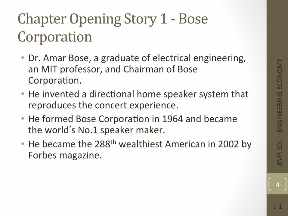
Chapter Opening Story 1 -‐ Bose Corporation •  Dr. Amar Bose, a graduate of electrical engineering, an MIT professor, and Chairman of Bose CorporaFon.

•  He invented a direcFonal home speaker system that reproduces the concert experience.

•  He formed Bose CorporaFon in 1964 and became the world’s No.1 speaker maker.

•  He became the 288th wealthiest American in 2002 by Forbes magazine.

EMR 301 – EN

GINEERING EC

ONOMY

L-‐1

4

5

Opening Story 2: Google

6

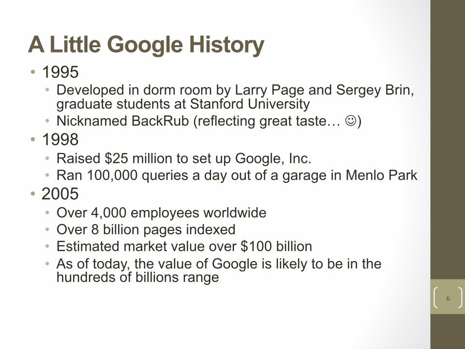
A Little Google History •  1995

•  Developed in dorm room by Larry Page and Sergey Brin, graduate students at Stanford University

•  Nicknamed BackRub (reflecting great taste… J) •  1998

•  Raised $25 million to set up Google, Inc. •  Ran 100,000 queries a day out of a garage in Menlo Park

•  2005 •  Over 4,000 employees worldwide •  Over 8 billion pages indexed •  Estimated market value over $100 billion •  As of today, the value of Google is likely to be in the

hundreds of billions range

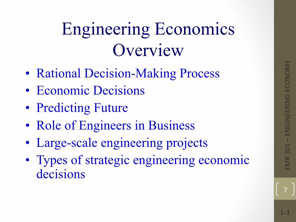
Engineering Economics Overview

•  Rational Decision-Making Process •  Economic Decisions •  Predicting Future •  Role of Engineers in Business •  Large-scale engineering projects •  Types of strategic engineering economic

decisions EMR 301 – EN

GINEERING EC

ONOMY

L-‐1

7

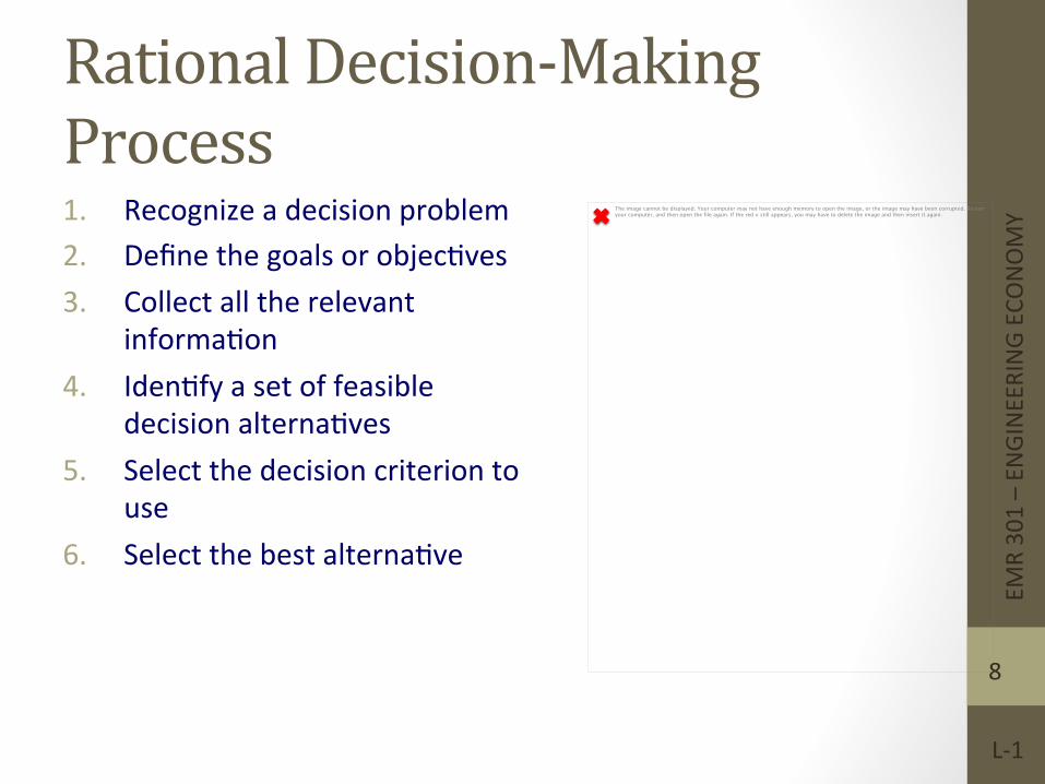
Rational Decision-‐Making Process 1.  Recognize a decision problem 2.  Define the goals or objecFves 3.  Collect all the relevant

informaFon 4.  IdenFfy a set of feasible

decision alternaFves 5.  Select the decision criterion to

use 6.  Select the best alternaFve

The image cannot be displayed. Your computer may not have enough memory to open the image, or the image may have been corrupted. Restart your computer, and then open the file again. If the red x still appears, you may have to delete the image and then insert it again.

EMR 301 – EN

GINEERING EC

ONOMY

L-‐1

8

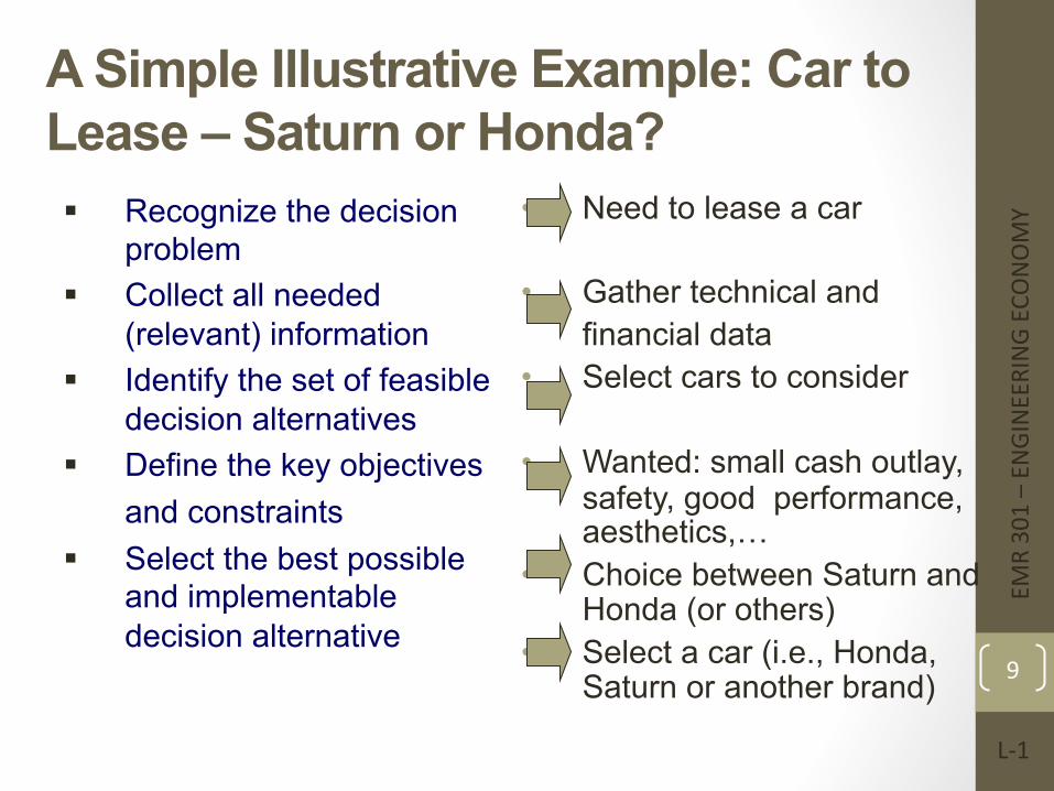
A Simple Illustrative Example: Car to Lease – Saturn or Honda? §  Recognize the decision

problem §  Collect all needed

(relevant) information §  Identify the set of feasible

decision alternatives §  Define the key objectives

and constraints §  Select the best possible

and implementable decision alternative

•  Need to lease a car

•  Gather technical and financial data

•  Select cars to consider

•  Wanted: small cash outlay, safety, good performance, aesthetics,…

•  Choice between Saturn and Honda (or others)

•  Select a car (i.e., Honda, Saturn or another brand)

EMR 301 – EN

GINEERING EC

ONOMY

L-‐1

9

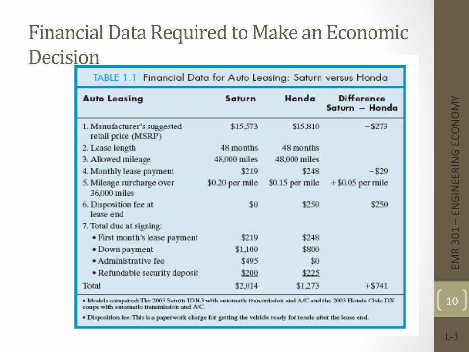
Financial Data Required to Make an Economic Decision

EMR 301 – EN

GINEERING EC

ONOMY

L-‐1

10

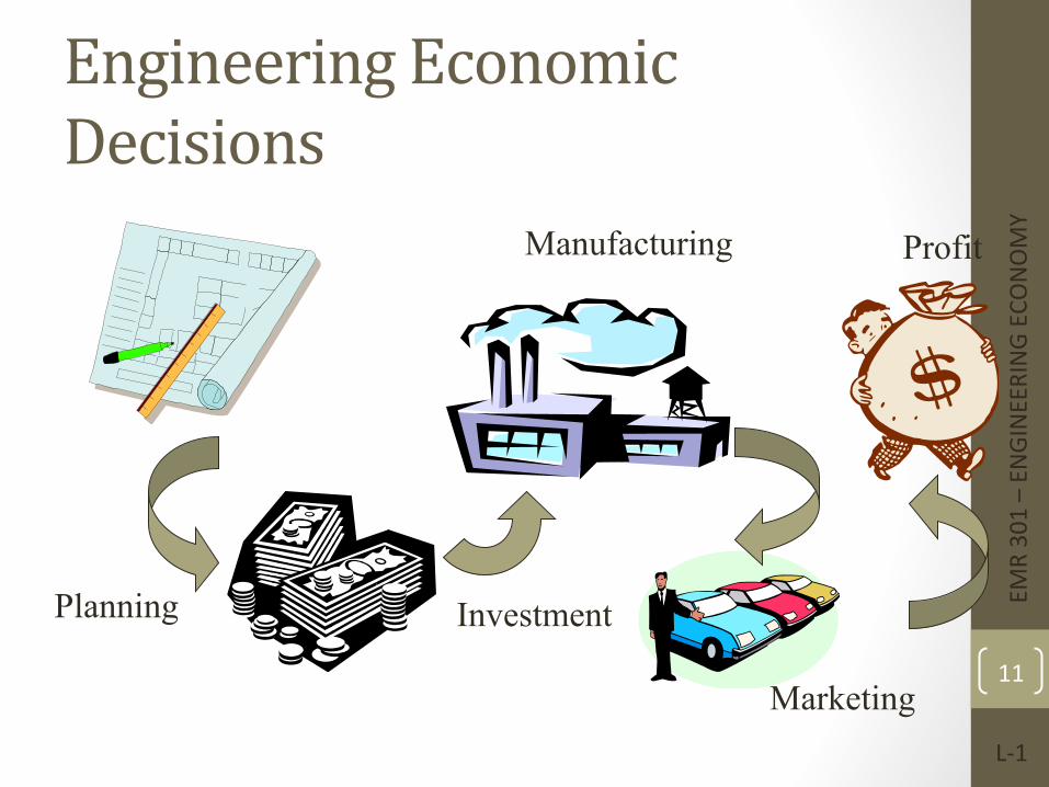
Engineering Economic Decisions

Planning Investment

Marketing

Profit Manufacturing

EMR 301 – EN

GINEERING EC

ONOMY

L-‐1

11

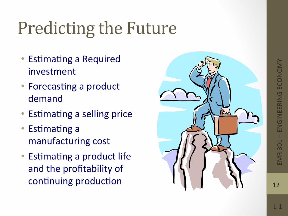
Predicting the Future •  EsFmaFng a Required investment

•  ForecasFng a product demand

•  EsFmaFng a selling price •  EsFmaFng a manufacturing cost

•  EsFmaFng a product life and the profitability of conFnuing producFon

EMR 301 – EN

GINEERING EC

ONOMY

L-‐1

12

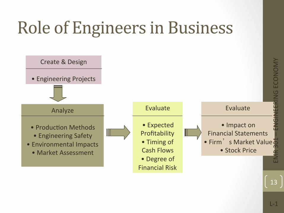
Create & Design

•  Engineering Projects

Evaluate

•  Expected Profitability •  Timing of Cash Flows •  Degree of Financial Risk

Analyze

•  ProducFon Methods •  Engineering Safety

•  Environmental Impacts •  Market Assessment

Evaluate

•  Impact on Financial Statements

•  Firm’s Market Value •  Stock Price

Role of Engineers in Business

EMR 301 – EN

GINEERING EC

ONOMY

L-‐1

13

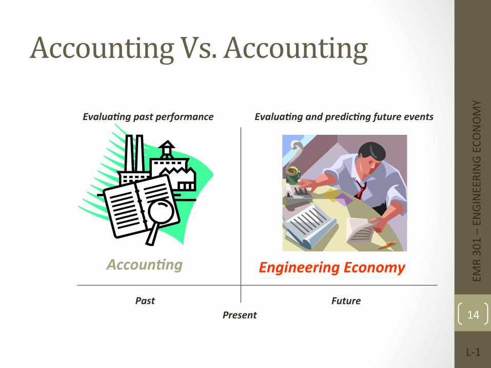
Present Future Past

Engineering Economy Accoun3ng

Evalua3ng past performance Evalua3ng and predic3ng future events

Accounting Vs. Accounting

EMR 301 – EN

GINEERING EC

ONOMY

L-‐1

14

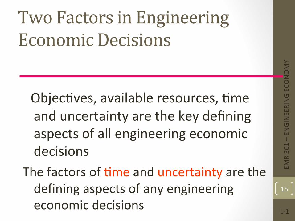
Two Factors in Engineering Economic Decisions

ObjecFves, available resources, Fme and uncertainty are the key defining aspects of all engineering economic decisions

The factors of Fme and uncertainty are the defining aspects of any engineering economic decisions

EMR 301 – EN

GINEERING EC

ONOMY

L-‐1

15

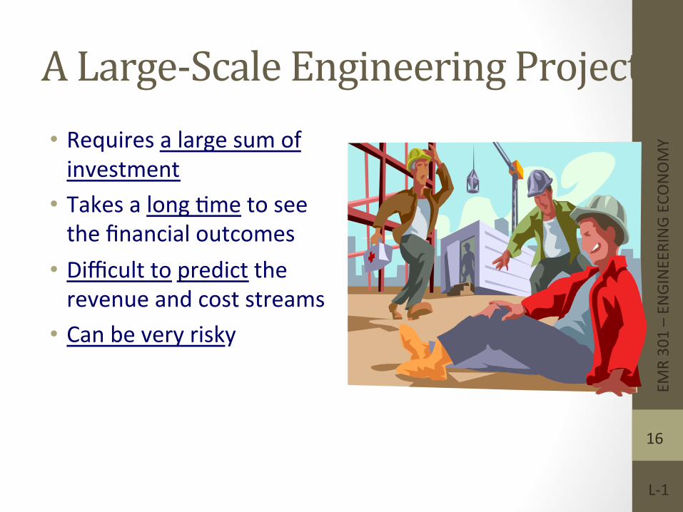
A Large-‐Scale Engineering Project •  Requires a large sum of investment

•  Takes a long Fme to see the financial outcomes

•  Difficult to predict the revenue and cost streams

•  Can be very risky

EMR 301 – EN

GINEERING EC

ONOMY

L-‐1

16

Types of Strategic Engineering Economic Decisions in Manufacturing Sector q Service Improvement q Equipment and Process SelecFon q Equipment Replacement q New Product and Product Expansion q Cost ReducFon q Profit MaximizaFon

Engineers have to make decisions unders resource constraints, and in presence of uncertainty.

EMR 301 – EN

GINEERING EC

ONOMY

L-‐1

17

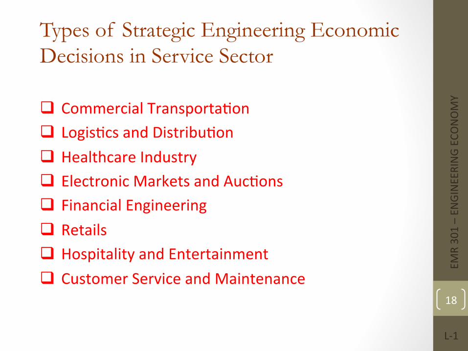
Types of Strategic Engineering Economic Decisions in Service Sector

q  Commercial TransportaFon q  LogisFcs and DistribuFon q  Healthcare Industry q  Electronic Markets and AucFons q  Financial Engineering q  Retails q  Hospitality and Entertainment q  Customer Service and Maintenance

EMR 301 – EN

GINEERING EC

ONOMY

L-‐1

18

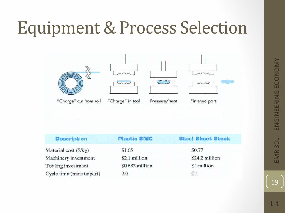
Equipment & Process Selection

EMR 301 – EN

GINEERING EC

ONOMY

L-‐1

19

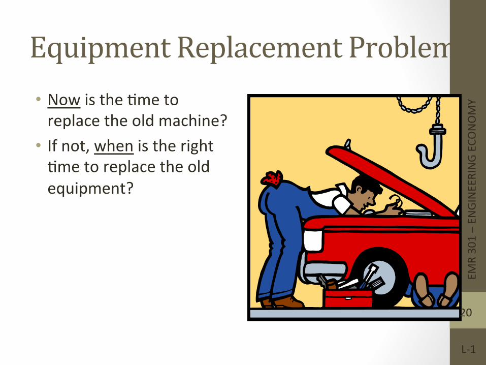
Equipment Replacement Problem •  Now is the Fme to replace the old machine?

•  If not, when is the right Fme to replace the old equipment?

EMR 301 – EN

GINEERING EC

ONOMY

L-‐1

20

New Product and Product Expansion •  Shall we build or acquire a new facility to meet the increased demand?

•  Is it worth spending money to market a new product?

EMR 301 – EN

GINEERING EC

ONOMY

L-‐1

21

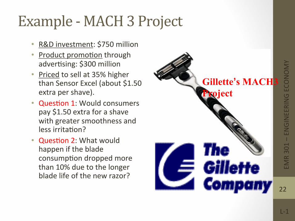
Example -‐ MACH 3 Project •  R&D investment: $750 million •  Product promoFon through adverFsing: $300 million

•  Priced to sell at 35% higher than Sensor Excel (about $1.50 extra per shave).

•  QuesFon 1: Would consumers pay $1.50 extra for a shave with greater smoothness and less irritaFon?

•  QuesFon 2: What would happen if the blade consumpFon dropped more than 10% due to the longer blade life of the new razor?

Gillette’s MACH3 Project

EMR 301 – EN

GINEERING EC

ONOMY

L-‐1

22

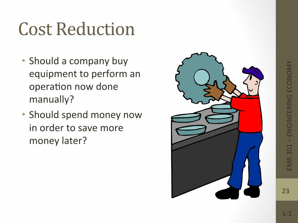
Cost Reduction •  Should a company buy equipment to perform an operaFon now done manually?

•  Should spend money now in order to save more money later?

EMR 301 – EN

GINEERING EC

ONOMY

L-‐1

23

Fundamental Principles of Engineering Economics •  Principle 1: An instant (nearby) dollar is worth more than a distant dollar

•  Principle 2: All it counts is the differences among alterna=ves •  Principle 3: Marginal revenue must exceed marginal cost •  Principle 4: Addi=onal risk is not taken without the expected addi=onal return

EMR 301 – EN

GINEERING EC

ONOMY

L-‐1

24

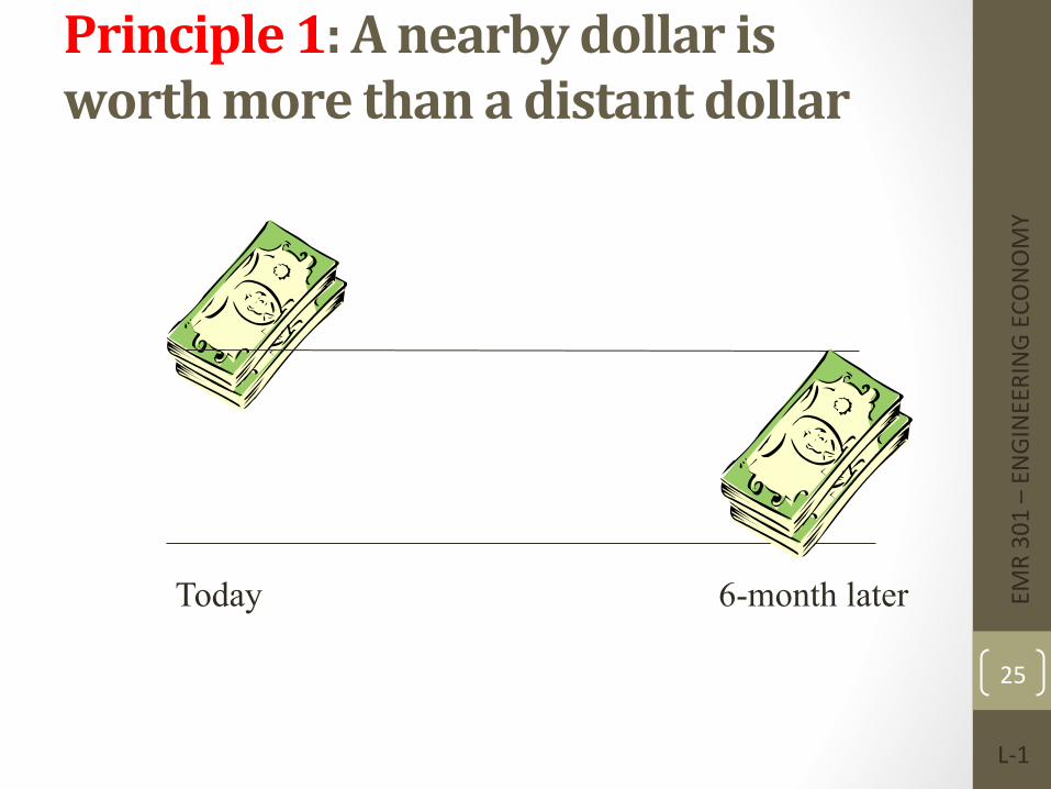
Principle 1: A nearby dollar is worth more than a distant dollar

Today 6-month later EMR 301 – EN

GINEERING EC

ONOMY

L-‐1

25

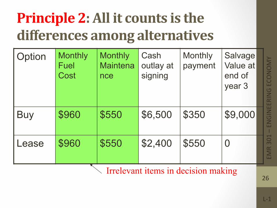
Principle 2: All it counts is the differences among alternatives Option Monthly

Fuel Cost

Monthly Maintenance

Cash outlay at signing

Monthly payment

Salvage Value at end of year 3

Buy $960 $550 $6,500 $350 $9,000

Lease $960 $550 $2,400 $550 0

Irrelevant items in decision making

EMR 301 – EN

GINEERING EC

ONOMY

L-‐1

26

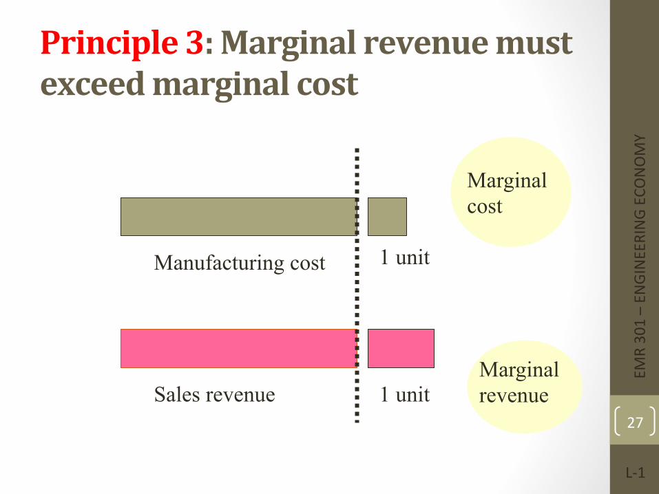
Principle 3: Marginal revenue must exceed marginal cost

Manufacturing cost

Sales revenue Marginal revenue

Marginal cost

1 unit

1 unit

EMR 301 – EN

GINEERING EC

ONOMY

L-‐1

27

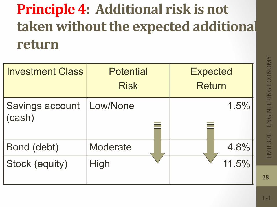
Principle 4: Additional risk is not taken without the expected additional return

Investment Class Potential Risk

Expected Return

Savings account (cash)

Low/None 1.5%

Bond (debt) Moderate 4.8% Stock (equity) High 11.5%

EMR 301 – EN

GINEERING EC

ONOMY

L-‐1

28

Summary •  The term engineering economic decision refers to all investment decisions relaFng to engineering projects.

•  The five main types of engineering economic decisions are •  (1) service improvement, •  (2) equipment and process selecFon, •  (3) equipment replacement, •  (4) new product and product expansion, and •  (5) cost reducFon.

•  The factors of Fme and uncertainty are the defining aspects of any investment project.

EMR 301 – EN

GINEERING EC

ONOMY

L-‐1

29

Time Value of Money (TVM) Description: TVM explains the change in the amount of money over time

for funds owed by or owned by a corporation (or individual)

•  Corporate investments are expected to earn a return •  Investment involves money •  Money has a ‘time value’

The time value of money is the most important concept in engineering economy

EMR 301 – EN

GINEERING EC

ONOMY

L-‐1

30

Engineering Economy •  Engineering Economy involves

•  Formulating •  Estimating, and •  Evaluating expected economic outcomes of alternatives designed to accomplish a

defined purpose •  Easy-to-use math techniques simplify the evaluation •  Estimates of economic outcomes can be deterministic or stochastic in

nature

EMR 301 – EN

GINEERING EC

ONOMY

L-‐1

31

General Steps for Decision Making Processes

1.  Understand the problem – define objectives 2.  Collect relevant information 3.  Define the set of feasible alternatives 4.  Identify the criteria for decision making 5.  Evaluate the alternatives and apply sensitivity analysis 6.  Select the “best” alternative 7.  Implement the alternative and monitor results

EMR 301 – EN

GINEERING EC

ONOMY

L-‐1

32

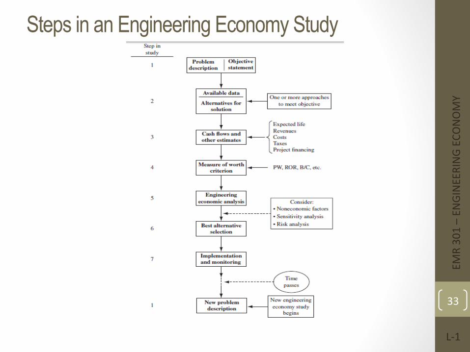
Steps in an Engineering Economy Study

EMR 301 – EN

GINEERING EC

ONOMY

L-‐1

33

Ethics – Different Levels Ø  Universal morals or ethics – Fundamental beliefs: stealing, lying,

harming or murdering another are wrong Ø Personal morals or ethics – Beliefs that an individual has and maintains

over time; how a universal moral is interpreted and used by each person

Ø  Professional or engineering ethics – Formal standard or code that guides a person in work activities and decision making

EMR 301 – EN

GINEERING EC

ONOMY

L-‐1

34

Code of Ethics for Engineers All disciplines have a formal code of ethics. National Society of Professional Engineers (NSPE) maintains a code specifically for engineers; many engineering professional societies have their own code

EMR 301 – EN

GINEERING EC

ONOMY

L-‐1

35

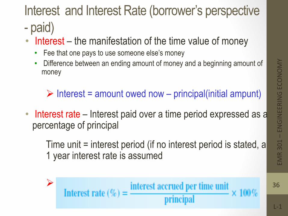
Interest and Interest Rate (borrower’s perspective - paid) •  Interest – the manifestation of the time value of money

•  Fee that one pays to use someone else’s money •  Difference between an ending amount of money and a beginning amount of

money

Ø  Interest = amount owed now – principal(initial ampunt)

•  Interest rate – Interest paid over a time period expressed as a percentage of principal

Time unit = interest period (if no interest period is stated, a 1 year interest rate is assumed Ø 

EMR 301 – EN

GINEERING EC

ONOMY

L-‐1

36

Interest and Interest Rate (borrower’s perspective - paid)

EMR 301 – EN

GINEERING EC

ONOMY

L-‐1

37

•  Example 1

•  Example 2

Rate of Return – ROR / Retorn on Investment -ROI (saver / lender / investor’s perspective - earned)

q  Interest earned over a period of Fme is expressed as a percentage of the original amount (principal)

interest accrued per time unitRate of return (%) = x 100%

original amount

v  Borrower’s perspective – interest rate paid

v  Lender’s or investor’s perspective – rate of return earned

EMR 301 – EN

GINEERING EC

ONOMY

L-‐1

38

Rate of Return – ROR / Retorn on Investment -ROI (saver / lender / investor’s perspective - earned)

EMR 301 – EN

GINEERING EC

ONOMY

L-‐1

39

•  Example 3

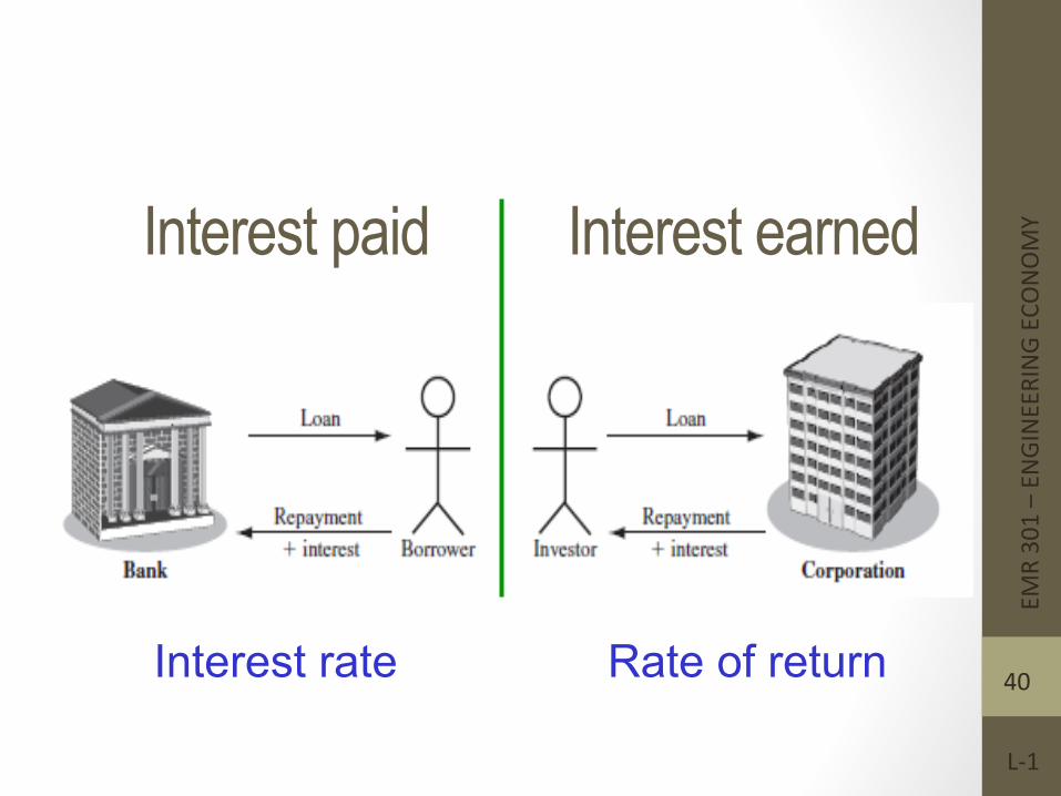
Interest paid Interest earned

Interest rate Rate of return

EMR 301 – EN

GINEERING EC

ONOMY

L-‐1

40

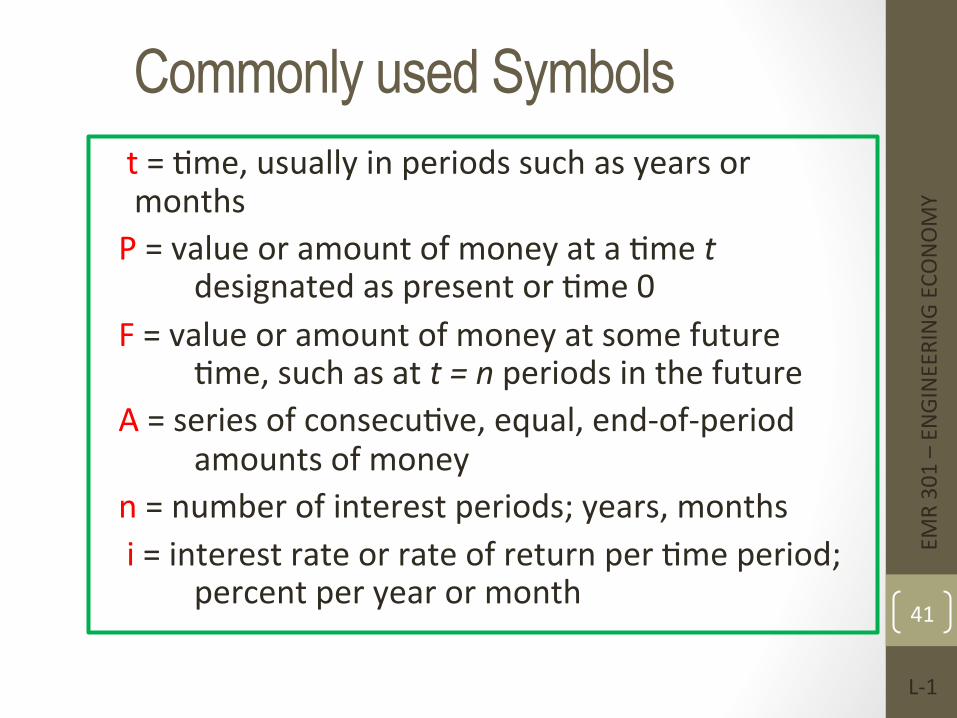
Commonly used Symbols t = Fme, usually in periods such as years or months

P = value or amount of money at a Fme t designated as present or Fme 0

F = value or amount of money at some future Fme, such as at t = n periods in the future

A = series of consecuFve, equal, end-‐of-‐period amounts of money

n = number of interest periods; years, months i = interest rate or rate of return per Fme period;

percent per year or month

EMR 301 – EN

GINEERING EC

ONOMY

L-‐1

41

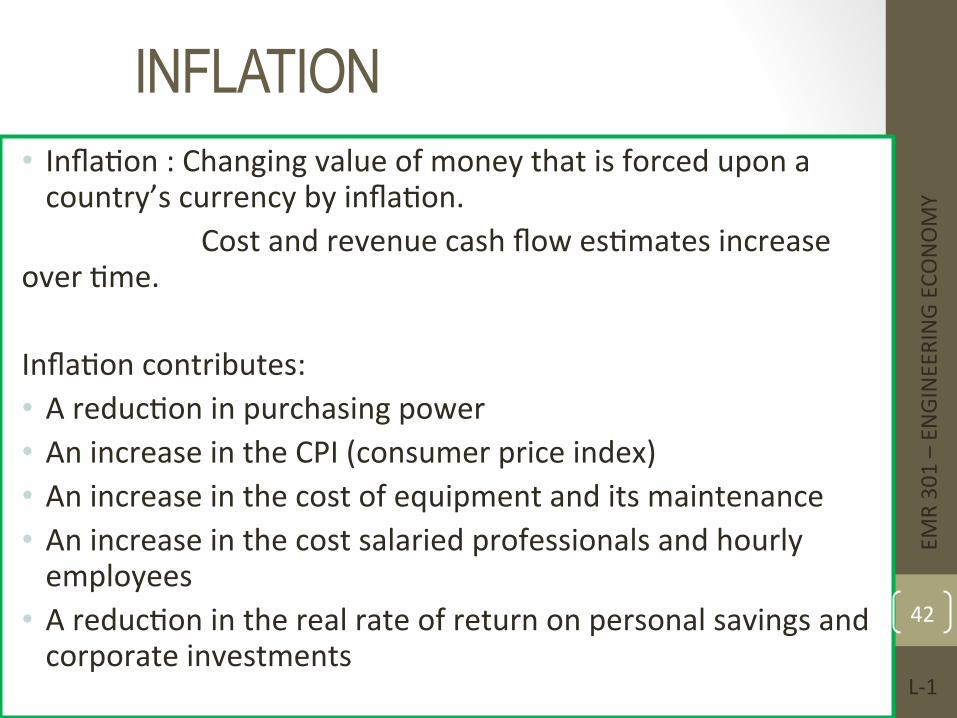
INFLATION •  InflaFon : Changing value of money that is forced upon a country’s currency by inflaFon.

Cost and revenue cash flow esFmates increase over Fme. InflaFon contributes: •  A reducFon in purchasing power •  An increase in the CPI (consumer price index) •  An increase in the cost of equipment and its maintenance •  An increase in the cost salaried professionals and hourly employees

•  A reducFon in the real rate of return on personal savings and corporate investments

EMR 301 – EN

GINEERING EC

ONOMY

L-‐1

42

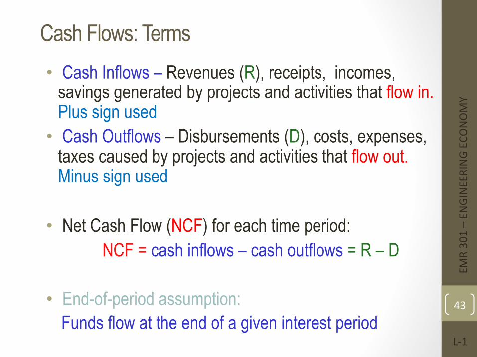
Cash Flows: Terms •  Cash Inflows – Revenues (R), receipts, incomes,

savings generated by projects and activities that flow in. Plus sign used

•  Cash Outflows – Disbursements (D), costs, expenses, taxes caused by projects and activities that flow out. Minus sign used

•  Net Cash Flow (NCF) for each time period:

NCF = cash inflows – cash outflows = R – D

•  End-of-period assumption: Funds flow at the end of a given interest period

EMR 301 – EN

GINEERING EC

ONOMY

L-‐1

43

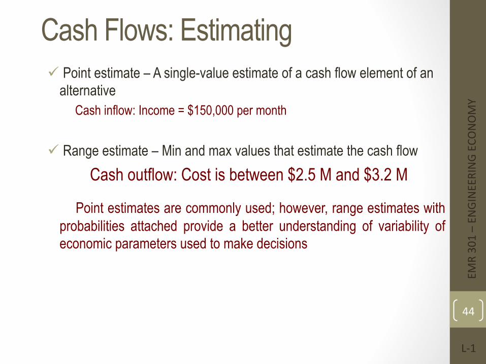
Cash Flows: Estimating ü  Point estimate – A single-value estimate of a cash flow element of an

alternative Cash inflow: Income = $150,000 per month

ü  Range estimate – Min and max values that estimate the cash flow

Cash outflow: Cost is between $2.5 M and $3.2 M

Point estimates are commonly used; however, range estimates with probabilities attached provide a better understanding of variability of economic parameters used to make decisions

EMR 301 – EN

GINEERING EC

ONOMY

L-‐1

44

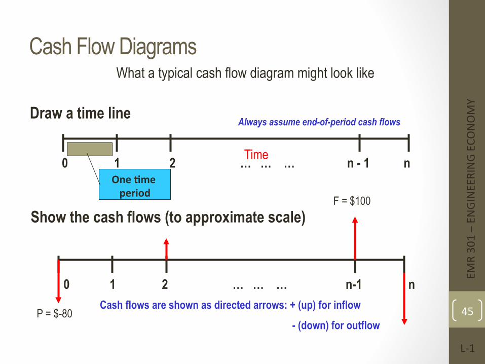
Cash Flow Diagrams What a typical cash flow diagram might look like

0 1 2 … … … n - 1 n

Draw a time line

One =me period

0 1 2 … … … n-1 n

Show the cash flows (to approximate scale)

Cash flows are shown as directed arrows: + (up) for inflow

- (down) for outflow

Always assume end-of-period cash flows

Time

F = $100

P = $-80

EMR 301 – EN

GINEERING EC

ONOMY

L-‐1

45

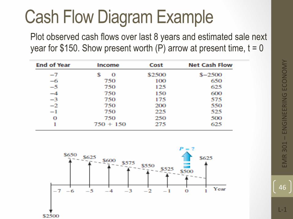
Cash Flow Diagram Example Plot observed cash flows over last 8 years and estimated sale next year for $150. Show present worth (P) arrow at present time, t = 0

EMR 301 – EN

GINEERING EC

ONOMY

L-‐1

46

Cash Flow Diagram

Example 4

EMR 301 – EN

GINEERING EC

ONOMY

L-‐1

47

Economic Equivalence Definition: Combination of interest rate (rate of return) and time value of

money to determine different amounts of money at different points in time that are economically equivalent

How it works: Use rate i and time t in upcoming relations to move money

(values of P, F and A) between time points t = 0, 1, …, n to make them equivalent (not equal) at the rate i

EMR 301 – EN

GINEERING EC

ONOMY

L-‐1

48

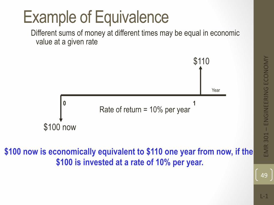
Example of Equivalence Different sums of money at different times may be equal in economic

value at a given rate

0 1

$100 now

$110

Rate of return = 10% per year

$100 now is economically equivalent to $110 one year from now, if the $100 is invested at a rate of 10% per year.

Year

EMR 301 – EN

GINEERING EC

ONOMY

L-‐1

49

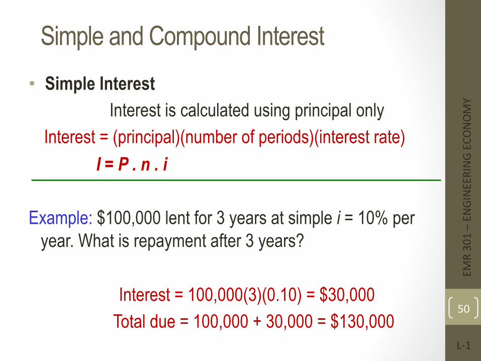
Simple and Compound Interest •  Simple Interest

Interest is calculated using principal only Interest = (principal)(number of periods)(interest rate) I = P . n . i

Example: $100,000 lent for 3 years at simple i = 10% per

year. What is repayment after 3 years? Interest = 100,000(3)(0.10) = $30,000 Total due = 100,000 + 30,000 = $130,000

EMR 301 – EN

GINEERING EC

ONOMY

L-‐1

50

Simple Interest

Example 5

EMR 301 – EN

GINEERING EC

ONOMY

L-‐1

51

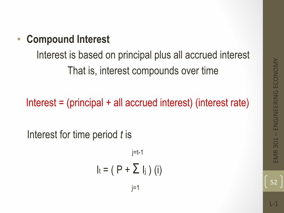
•  Compound Interest Interest is based on principal plus all accrued interest

That is, interest compounds over time Interest = (principal + all accrued interest) (interest rate)

Interest for time period t is

EMR 301 – EN

GINEERING EC

ONOMY

L-‐1

52

j=t-1

It = ( P + Σ Ij ) (i) j=1

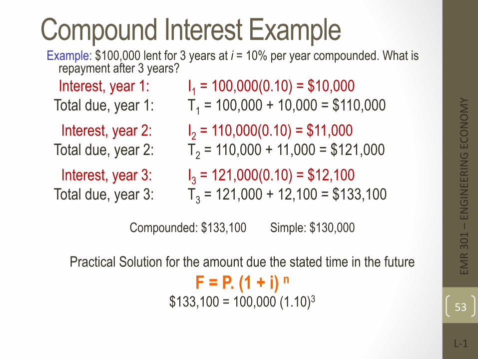
Compound Interest Example Example: $100,000 lent for 3 years at i = 10% per year compounded. What is

repayment after 3 years? Interest, year 1: I1 = 100,000(0.10) = $10,000

Total due, year 1: T1 = 100,000 + 10,000 = $110,000

Interest, year 2: I2 = 110,000(0.10) = $11,000 Total due, year 2: T2 = 110,000 + 11,000 = $121,000

Interest, year 3: I3 = 121,000(0.10) = $12,100 Total due, year 3: T3 = 121,000 + 12,100 = $133,100

Compounded: $133,100 Simple: $130,000

Practical Solution for the amount due the stated time in the future

F = P. (1 + i) n

$133,100 = 100,000 (1.10)3

EMR 301 – EN

GINEERING EC

ONOMY

L-‐1

53

Compound Interest

Example 6

EMR 301 – EN

GINEERING EC

ONOMY

L-‐1

54

© 20

12 by

McG

raw-

Hill,

New

York,

N.Y

All

Righ

ts Re

serve

d

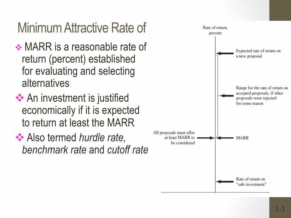
Minimum Attractive Rate of Return v  MARR is a reasonable rate of

return (percent) established for evaluating and selecting alternatives

v  An investment is justified economically if it is expected to return at least the MARR

v  Also termed hurdle rate, benchmark rate and cutoff rate

L-‐1

55

MARR Characteristics •  MARR is established by the financial managers of the firm •  MARR is fundamentally connected to the cost of capital •  Both types of capital financing are used to determine the weighted

average cost of capital (WACC) and the MARR •  MARR usually considers the risk inherent to a project

EMR 301 – EN

GINEERING EC

ONOMY

L-‐1

56

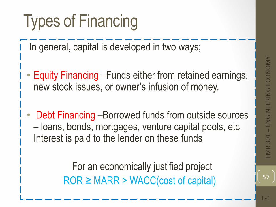
Types of Financing In general, capital is developed in two ways;

• Equity Financing –Funds either from retained earnings, new stock issues, or owner’s infusion of money.

•  Debt Financing –Borrowed funds from outside sources – loans, bonds, mortgages, venture capital pools, etc. Interest is paid to the lender on these funds

For an economically justified project

ROR ≥ MARR > WACC(cost of capital)

EMR 301 – EN

GINEERING EC

ONOMY

L-‐1

57

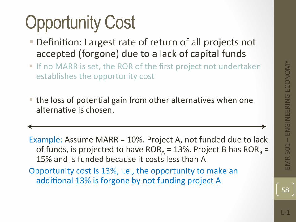
Opportunity Cost § DefiniFon: Largest rate of return of all projects not accepted (forgone) due to a lack of capital funds

§  If no MARR is set, the ROR of the first project not undertaken establishes the opportunity cost

§  the loss of potenFal gain from other alternaFves when one alternaFve is chosen.

Example: Assume MARR = 10%. Project A, not funded due to lack of funds, is projected to have RORA = 13%. Project B has RORB = 15% and is funded because it costs less than A

Opportunity cost is 13%, i.e., the opportunity to make an addiFonal 13% is forgone by not funding project A

EMR 301 – EN

GINEERING EC

ONOMY

L-‐1

58

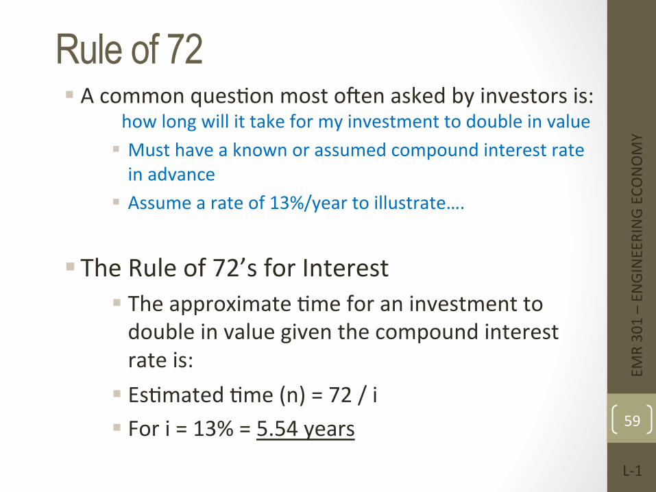
Rule of 72 § A common quesFon most oHen asked by investors is:

how long will it take for my investment to double in value § Must have a known or assumed compound interest rate in advance

§  Assume a rate of 13%/year to illustrate….

§ The Rule of 72’s for Interest § The approximate Fme for an investment to double in value given the compound interest rate is:

§ EsFmated Fme (n) = 72 / i § For i = 13% = 5.54 years

EMR 301 – EN

GINEERING EC

ONOMY

L-‐1

59

Rule of 72

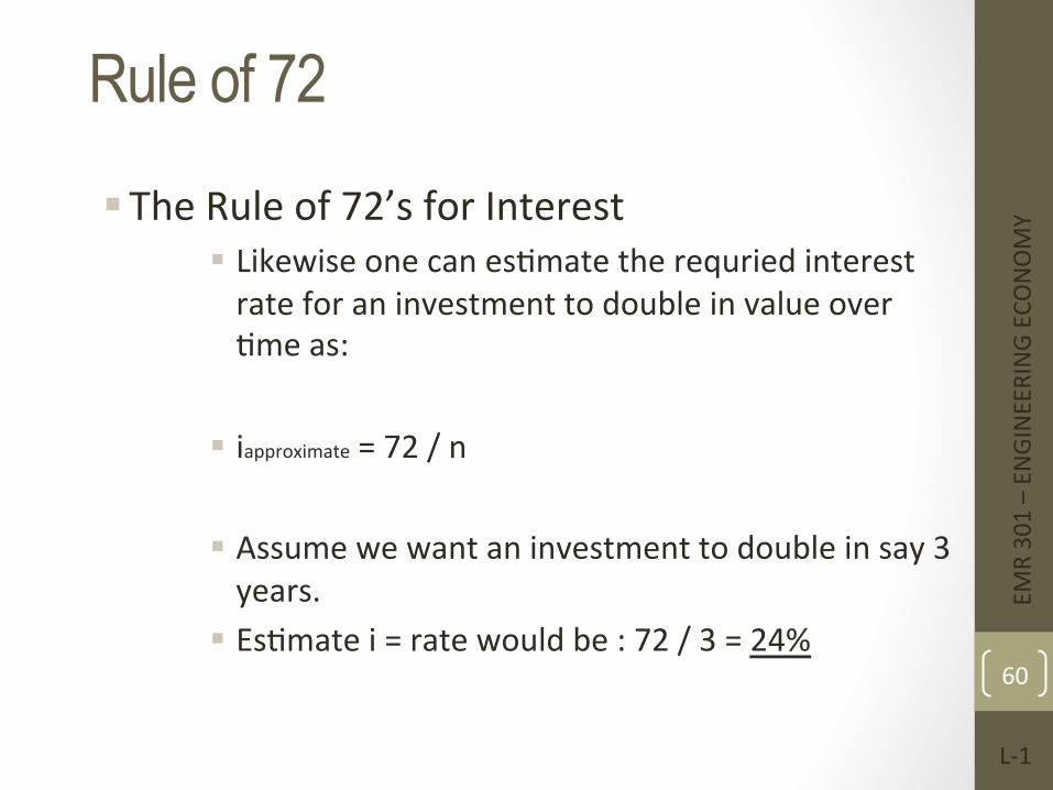
§ The Rule of 72’s for Interest §  Likewise one can esFmate the requried interest rate for an investment to double in value over Fme as:

§  iapproximate = 72 / n

§ Assume we want an investment to double in say 3 years.

§  EsFmate i = rate would be : 72 / 3 = 24%

EMR 301 – EN

GINEERING EC

ONOMY

L-‐1

60

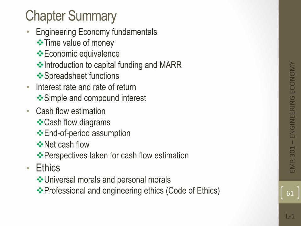
Chapter Summary •  Engineering Economy fundamentals

v Time value of money v Economic equivalence v Introduction to capital funding and MARR v Spreadsheet functions

•  Interest rate and rate of return v Simple and compound interest

•  Cash flow estimation v Cash flow diagrams v End-of-period assumption v Net cash flow v Perspectives taken for cash flow estimation

•  Ethics v Universal morals and personal morals v Professional and engineering ethics (Code of Ethics)

EMR 301 – EN

GINEERING EC

ONOMY

L-‐1

61

ENGINEERING ECONOMY

EMR 301 – EN

GINEERING EC

ONOMY

L-‐1

62

Factors : How Time and Interest Affect Money

© 20

12 by

McG

raw-

Hill,

New

York,

N.Y

All

Righ

ts Re

serve

d

1-63

Lecture slides to accompany

Engineering Economy 7th edition

Leland Blank Anthony Tarquin

Chapter 1 Foundations Of

Engineering Economy

© 20

12 by

McG

raw-

Hill,

New

York,

N.Y

All

Righ

ts Re

serve

d

1-64





Engineering Economy

© 20

12 by

McG

raw-

Hill,

New

York,

N.Y

All

Righ

ts Re

serve

d

1-65





Engineering Economy

© 20

12 by

McG

raw-

Hill,

New

York,

N.Y

All

Righ

ts Re

serve

d

1-66





Engineering Economy

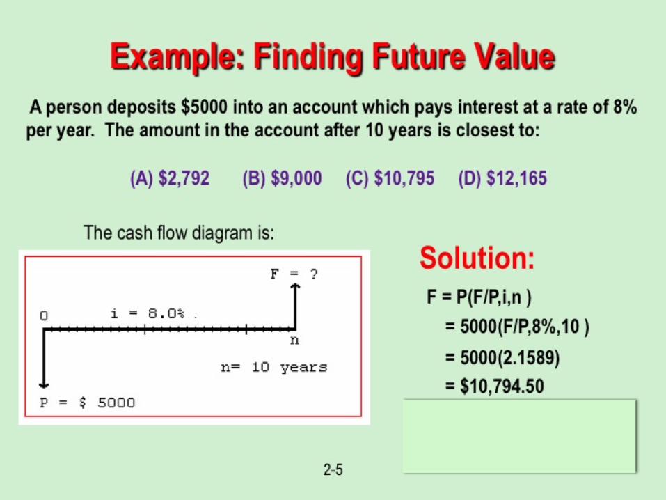
Finding Future Value

Example 6

EMR 301 – EN

GINEERING EC

ONOMY

L-‐1

67

© 20

12 by

McG

raw-

Hill,

New

York,

N.Y

All

Righ

ts Re

serve

d

1-68





Engineering Economy

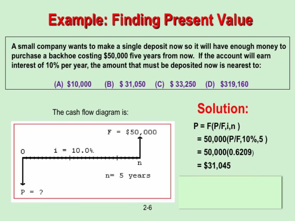
Finding Present Value

Example 7

EMR 301 – EN

GINEERING EC

ONOMY

L-‐1

69

Finding Present/Future Value

Example 8

EMR 301 – EN

GINEERING EC

ONOMY

L-‐1

70

© 20

12 by

McG

raw-

Hill,

New

York,

N.Y

All

Righ

ts Re

serve

d

1-71





Engineering Economy

© 20

12 by

McG

raw-

Hill,

New

York,

N.Y

All

Righ

ts Re

serve

d

1-72





Engineering Economy

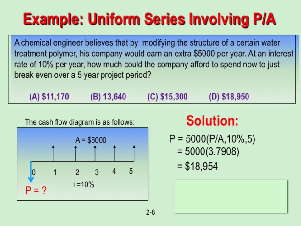
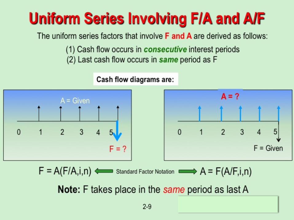
Uniform Series Involving P/A

Example 9

EMR 301 – EN

GINEERING EC

ONOMY

L-‐1

73

© 20

12 by

McG

raw-

Hill,

New

York,

N.Y

All

Righ

ts Re

serve

d

1-74





Engineering Economy

Uniform Series Involving F/A

Example 10 Example 11

EMR 301 – EN

GINEERING EC

ONOMY

L-‐1

75

© 20

12 by

McG

raw-

Hill,

New

York,

N.Y

All

Righ

ts Re

serve

d

1-76





Engineering Economy

© 20

12 by

McG

raw-

Hill,

New

York,

N.Y

All

Righ

ts Re

serve

d

1-77





Engineering Economy

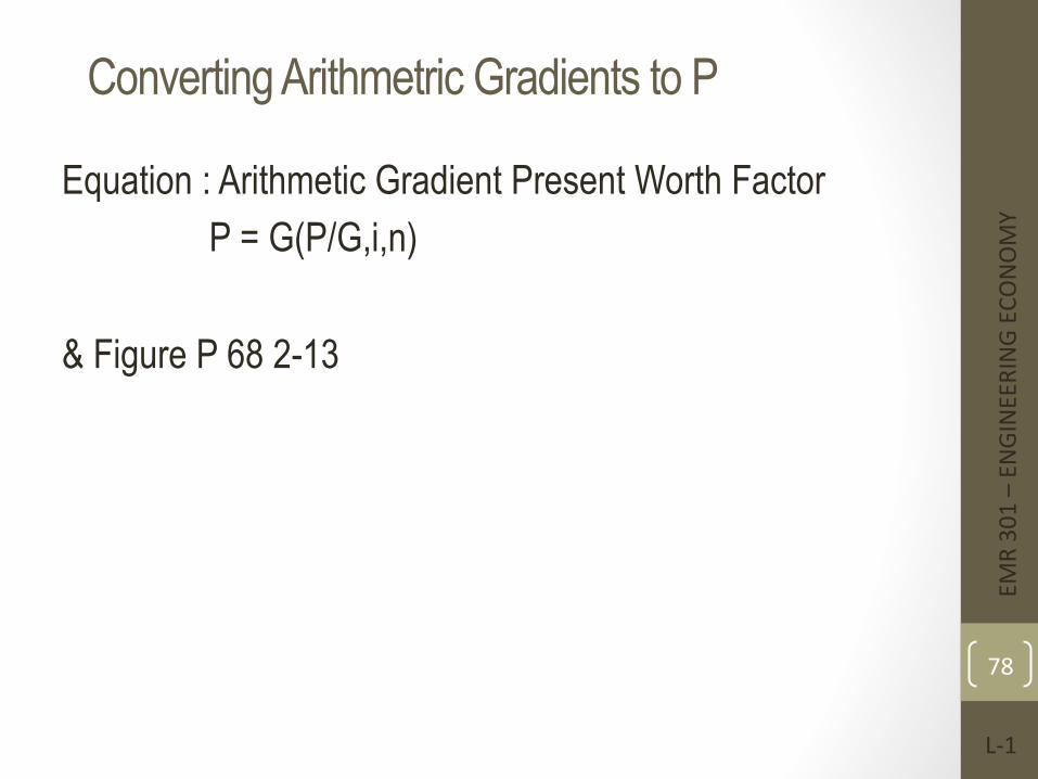
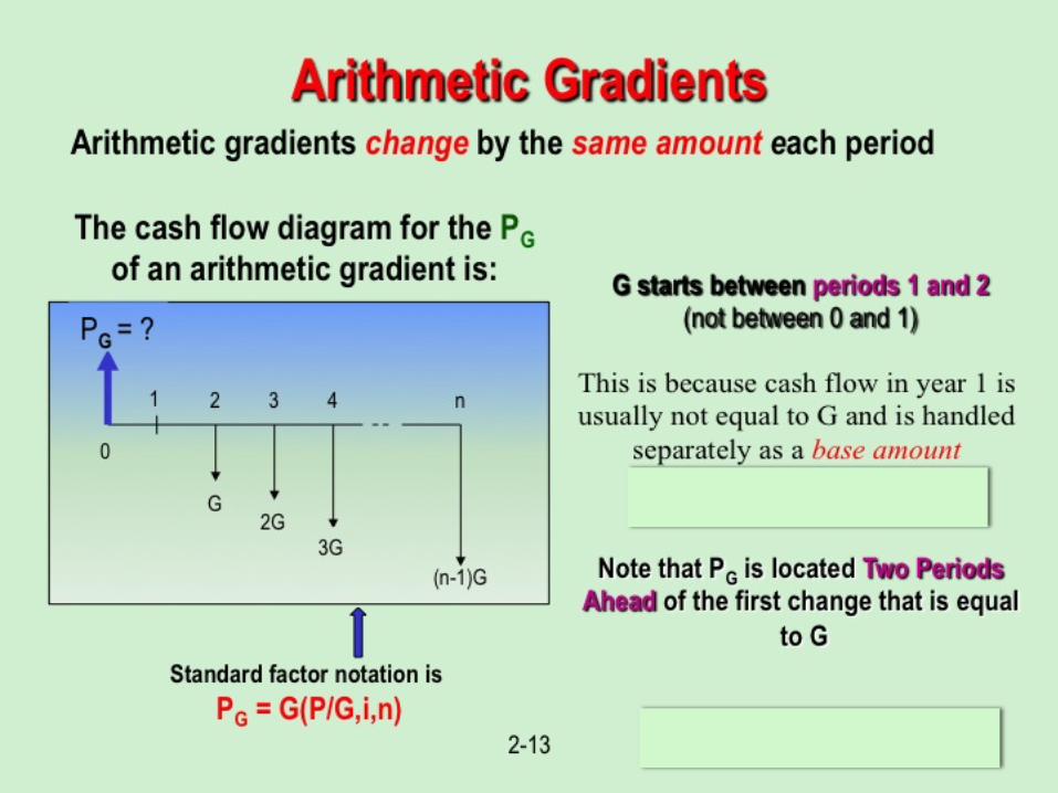
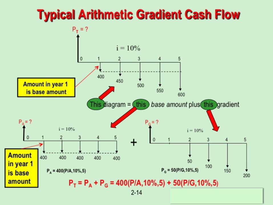
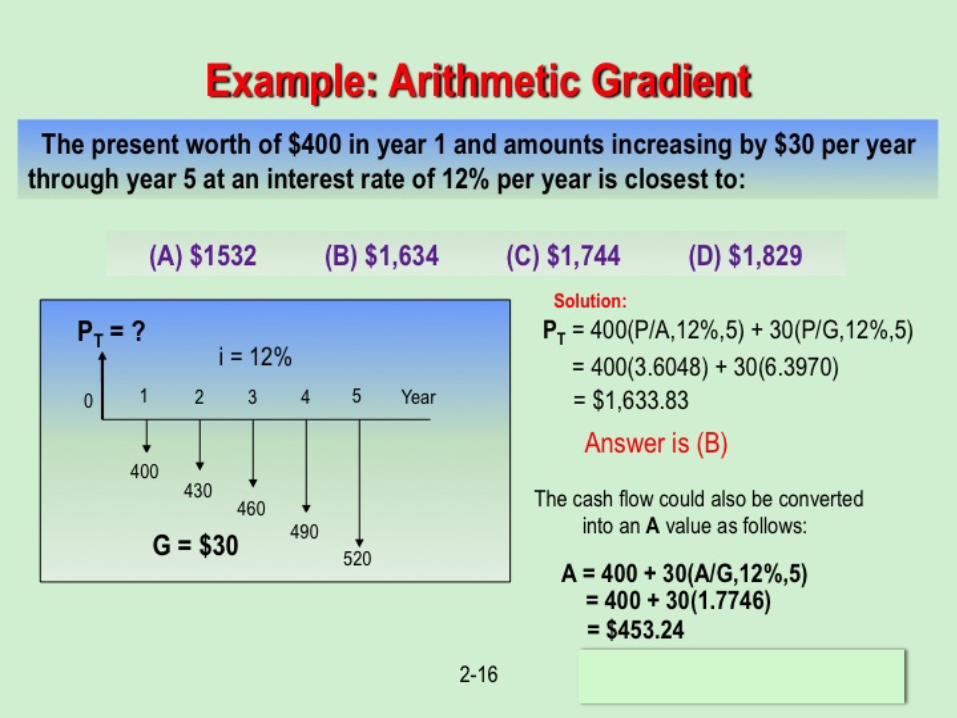
Converting Arithmetric Gradients to P

Equation : Arithmetic Gradient Present Worth Factor P = G(P/G,i,n) & Figure P 68 2-13

EMR 301 – EN

GINEERING EC

ONOMY

L-‐1

78

Arithmetric Gradients

Example 12

EMR 301 – EN

GINEERING EC

ONOMY

L-‐1

79

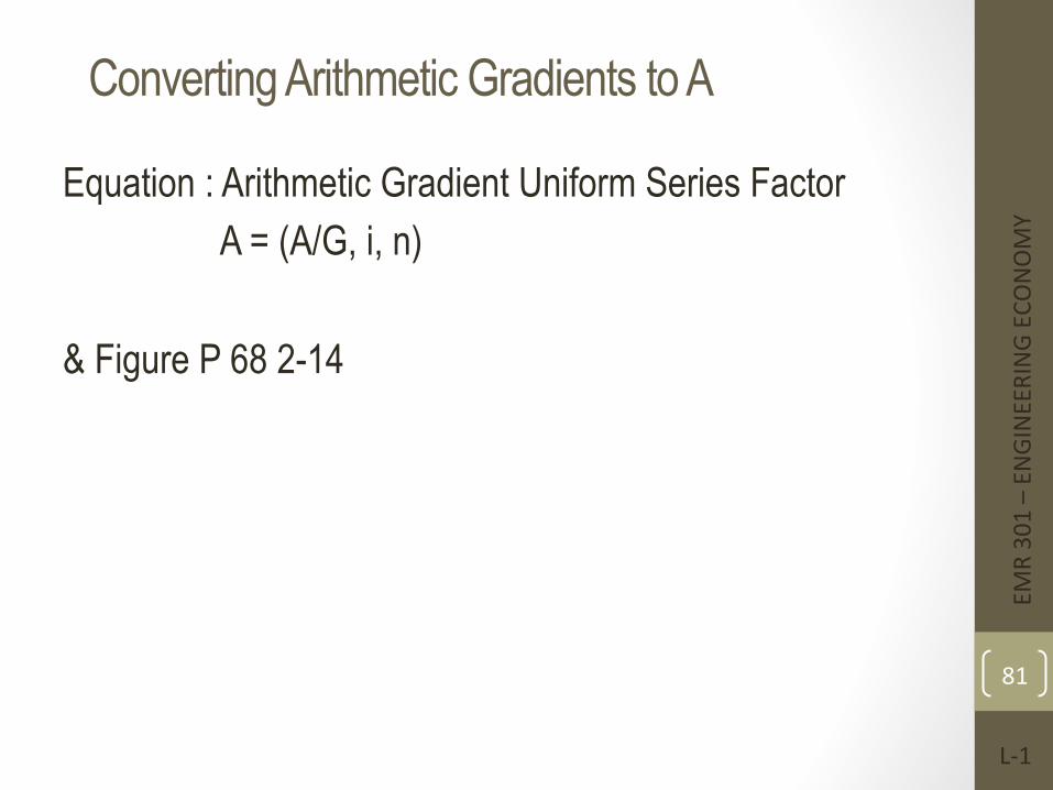
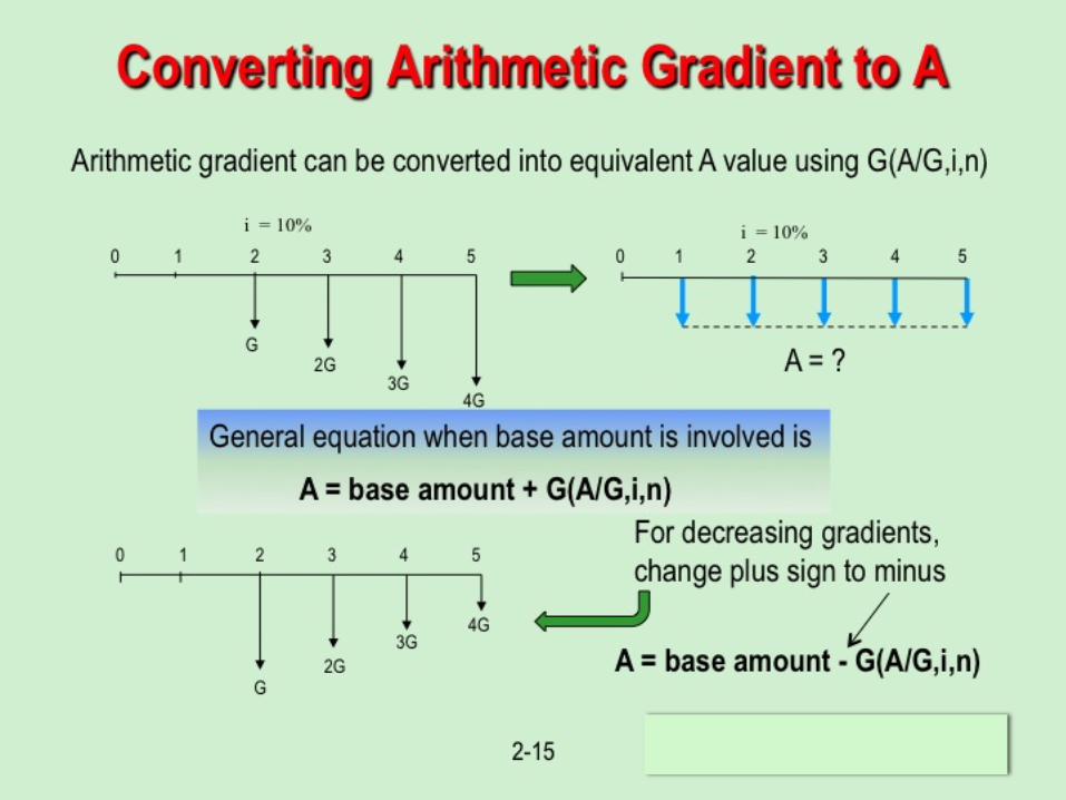
Converting Arithmetic Gradients to A

Equation : Arithmetic Gradient Uniform Series Factor A = (A/G, i, n) & Figure P 68 2-14

EMR 301 – EN

GINEERING EC

ONOMY

L-‐1

81

Arithmetric Gradients

Example 13

EMR 301 – EN

GINEERING EC

ONOMY

L-‐1

83

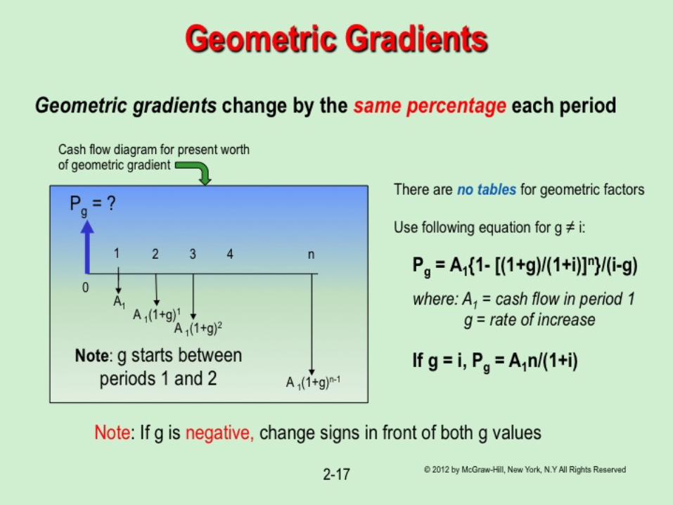
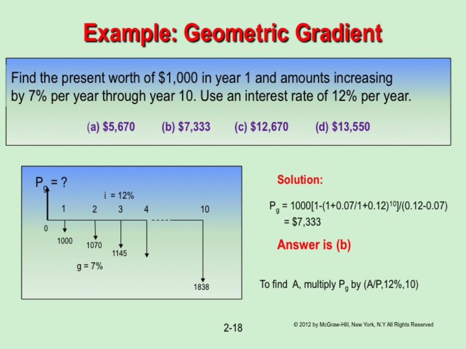
Geometric Gradients

Example 14

EMR 301 – EN

GINEERING EC

ONOMY

L-‐1

86

Example 15

EMR 301 – EN

GINEERING EC

ONOMY

L-‐1

88

Example 16

EMR 301 – EN

GINEERING EC

ONOMY

L-‐1

90

ENGINEERING ECONOMY

EMR 301 – EN

GINEERING EC

ONOMY

L-‐1

92

Combining Factors

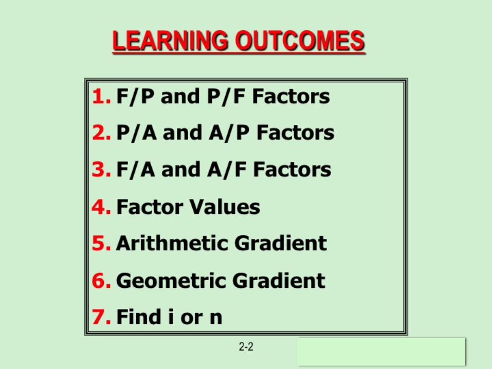
LEARNING OUTCOMES

1. Shifted uniform series

2. Shifted series and single cash flows

3. Shifted gradients

EMR 301 – EN

GINEERING EC

ONOMY

L-‐1

93

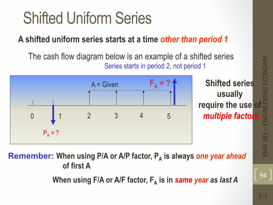
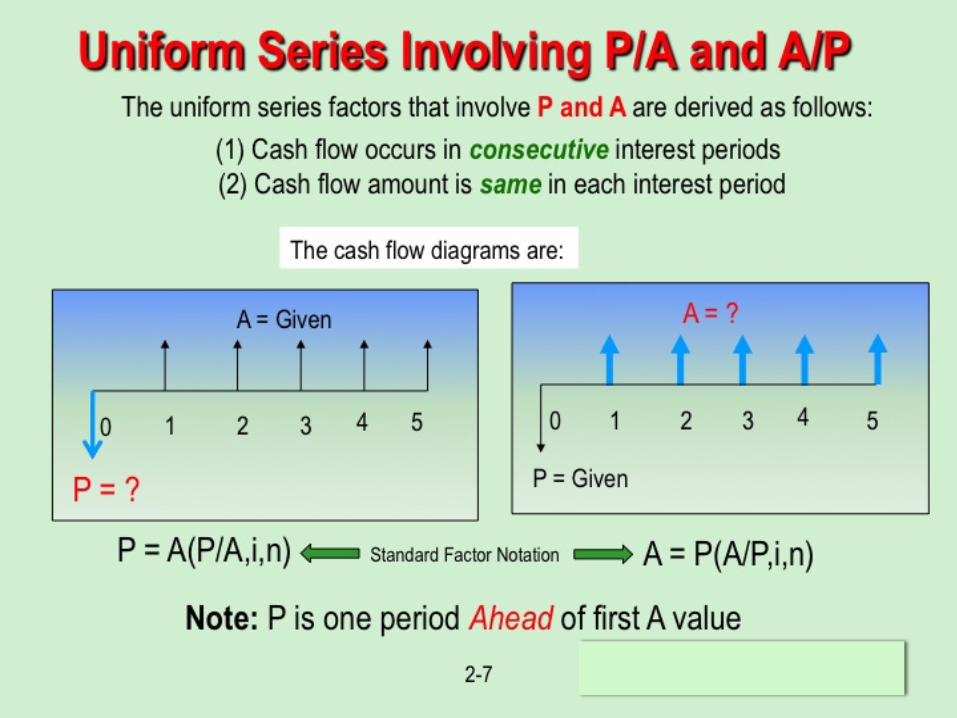
Shifted Uniform Series A shifted uniform series starts at a time other than period 1

0 1 2 3 4 5

A = Given

PA = ?

The cash flow diagram below is an example of a shifted series Series starts in period 2, not period 1

Shifted series usually

require the use of multiple factors

Remember: When using P/A or A/P factor, PA is always one year ahead of first A

When using F/A or A/F factor, FA is in same year as last A

FA = ?

EMR 301 – EN

GINEERING EC

ONOMY

L-‐1

94

Example Using P/A Factor: Shifted Uniform Series

P0 = ?

A = $10,000

0 1 2 3 4 5 6

i = 10%

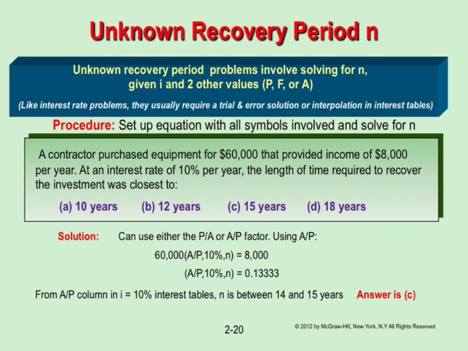
The present worth of the cash flow shown below at i = 10% is: (a) $25,304 (b) $29,562 (c) $34,462 (d) $37,908

Solution: (1) Use P/A factor with n = 5 (for 5 arrows) to get P1 in year 1 (2) Use P/F factor with n = 1 to move P1 back for P0 in year 0

P0 = P1(P/F,10%,1) = A(P/A,10%,5)(P/F,10%,1) = 10,000(3.7908)(0.9091) = $34,462 Answer is (c)

0 1 2 3 4 5

P1 = ?

Actual year Series year

EMR 301 – EN

GINEERING EC

ONOMY

L-‐1

95

Example 17

EMR 301 – EN

GINEERING EC

ONOMY

L-‐1

96

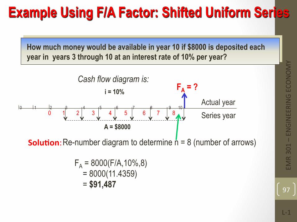
How much money would be available in year 10 if $8000 is deposited each year in years 3 through 10 at an interest rate of 10% per year?

0 1 2 3 4 5 6 7 8 9 10

FA = ?

A = $8000

i = 10%

Solu=on: Re-number diagram to determine n = 8 (number of arrows)

0 1 2 3 4 5 6 7 8

Cash flow diagram is:

FA = 8000(F/A,10%,8) = 8000(11.4359) = $91,487

Example Using F/A Factor: Shifted Uniform Series

Actual year Series year

EMR 301 – EN

GINEERING EC

ONOMY

L-‐1

97

Example 18

EMR 301 – EN

GINEERING EC

ONOMY

L-‐1

98

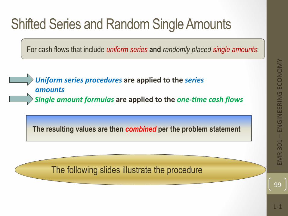
Shifted Series and Random Single Amounts For cash flows that include uniform series and randomly placed single amounts:

Uniform series procedures are applied to the series amounts Single amount formulas are applied to the one-‐3me cash flows

The resulting values are then combined per the problem statement

The following slides illustrate the procedure

EMR 301 – EN

GINEERING EC

ONOMY

L-‐1

99

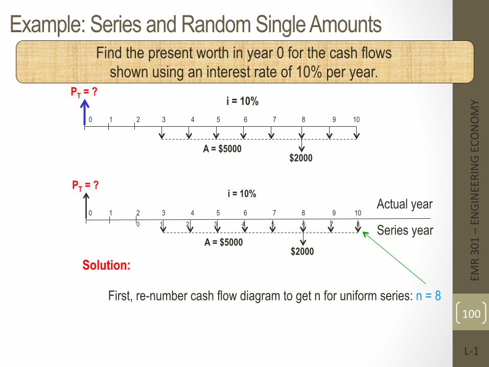
Example: Series and Random Single Amounts Find the present worth in year 0 for the cash flows

shown using an interest rate of 10% per year.

0 1 2 3 4 5 6 7 8 9 10

PT = ?

A = $5000

i = 10%

First, re-number cash flow diagram to get n for uniform series: n = 8

$2000

0 1 2 3 4 5 6 7 8 9 10

PT = ?

A = $5000

i = 10%

$2000

0 1 2 3 4 5 6 7 8

Solution:

Actual year

Series year

EMR 301 – EN

GINEERING EC

ONOMY

L-‐1

100

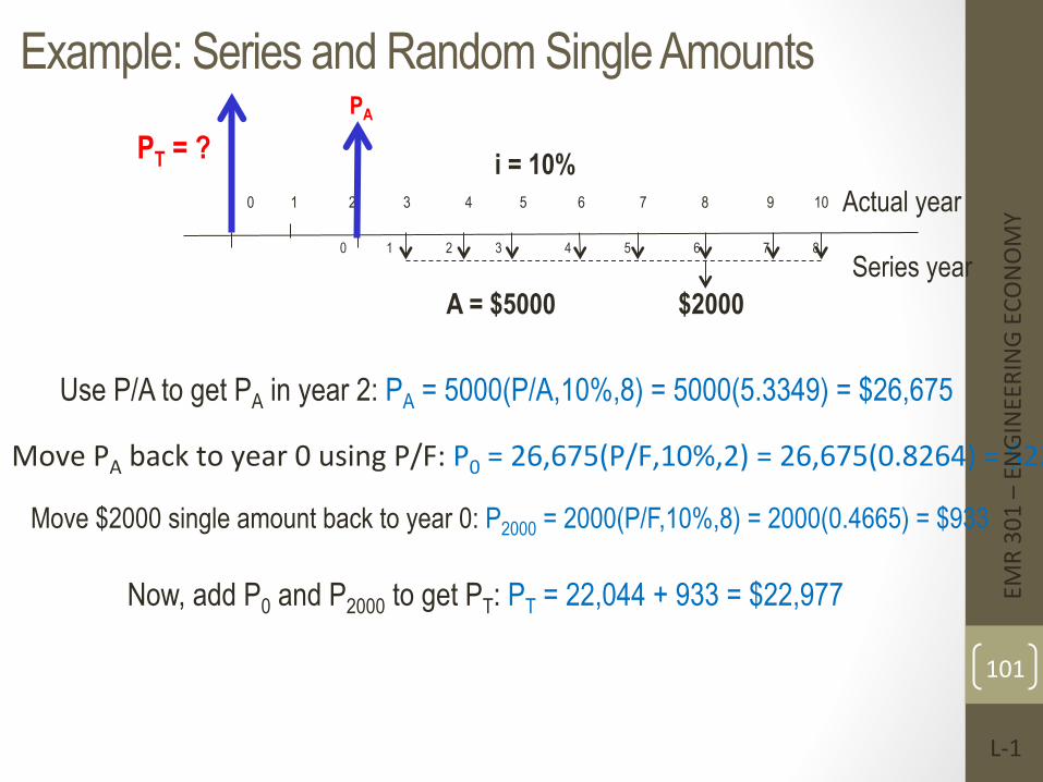
A = $5000

i = 10%

0 1 2 3 4 5 6 7 8

Actual year

Series year

0 1 2 3 4 5 6 7 8 9 10

$2000

Use P/A to get PA in year 2: PA = 5000(P/A,10%,8) = 5000(5.3349) = $26,675

Move PA back to year 0 using P/F: P0 = 26,675(P/F,10%,2) = 26,675(0.8264) = $22,044

Move $2000 single amount back to year 0: P2000 = 2000(P/F,10%,8) = 2000(0.4665) = $933

Now, add P0 and P2000 to get PT: PT = 22,044 + 933 = $22,977

Example: Series and Random Single Amounts

PT = ? PA

EMR 301 – EN

GINEERING EC

ONOMY

L-‐1

101

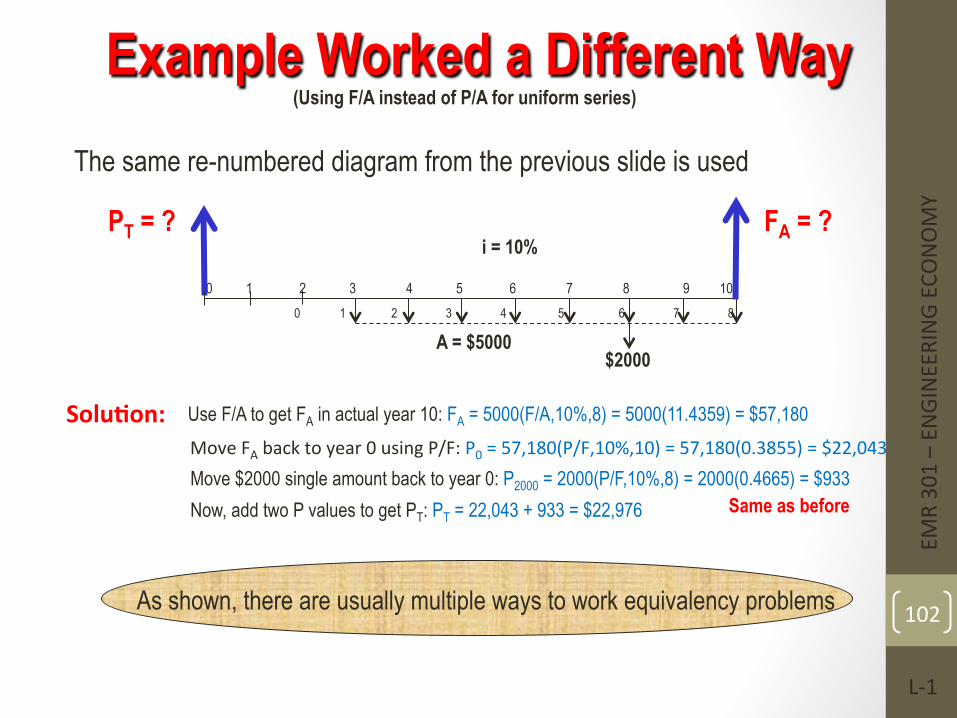
Example Worked a Different Way (Using F/A instead of P/A for uniform series)

0 1 2 3 4 5 6 7 8 9 10

PT = ?

A = $5000

i = 10%

$2000

0 1 2 3 4 5 6 7 8

The same re-numbered diagram from the previous slide is used

Solu=on: Use F/A to get FA in actual year 10: FA = 5000(F/A,10%,8) = 5000(11.4359) = $57,180

Move $2000 single amount back to year 0: P2000 = 2000(P/F,10%,8) = 2000(0.4665) = $933 Now, add two P values to get PT: PT = 22,043 + 933 = $22,976 Same as before

Move FA back to year 0 using P/F: P0 = 57,180(P/F,10%,10) = 57,180(0.3855) = $22,043

As shown, there are usually multiple ways to work equivalency problems

FA = ?

EMR 301 – EN

GINEERING EC

ONOMY

L-‐1

102

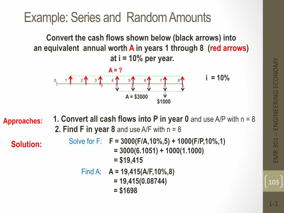
Example: Series and Random Amounts Convert the cash flows shown below (black arrows) into

an equivalent annual worth A in years 1 through 8 (red arrows) at i = 10% per year.

0 1 2 3 4 5 6 7 8

A = $3000

i = 10%

$1000

0 1 2 3 4 5

A = ?

Solution:

1. Convert all cash flows into P in year 0 and use A/P with n = 8 2. Find F in year 8 and use A/F with n = 8

Solve for F: F = 3000(F/A,10%,5) + 1000(F/P,10%,1) = 3000(6.1051) + 1000(1.1000) = $19,415

Find A: A = 19,415(A/F,10%,8) = 19,415(0.08744) = $1698

Approaches:

EMR 301 – EN

GINEERING EC

ONOMY

L-‐1

103

Example 19

EMR 301 – EN

GINEERING EC

ONOMY

L-‐1

104

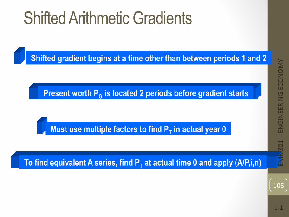
Shifted Arithmetic Gradients

Shifted gradient begins at a time other than between periods 1 and 2

Present worth PG is located 2 periods before gradient starts

Must use multiple factors to find PT in actual year 0

To find equivalent A series, find PT at actual time 0 and apply (A/P,i,n) EMR 301 – EN

GINEERING EC

ONOMY

L-‐1

105

3-106

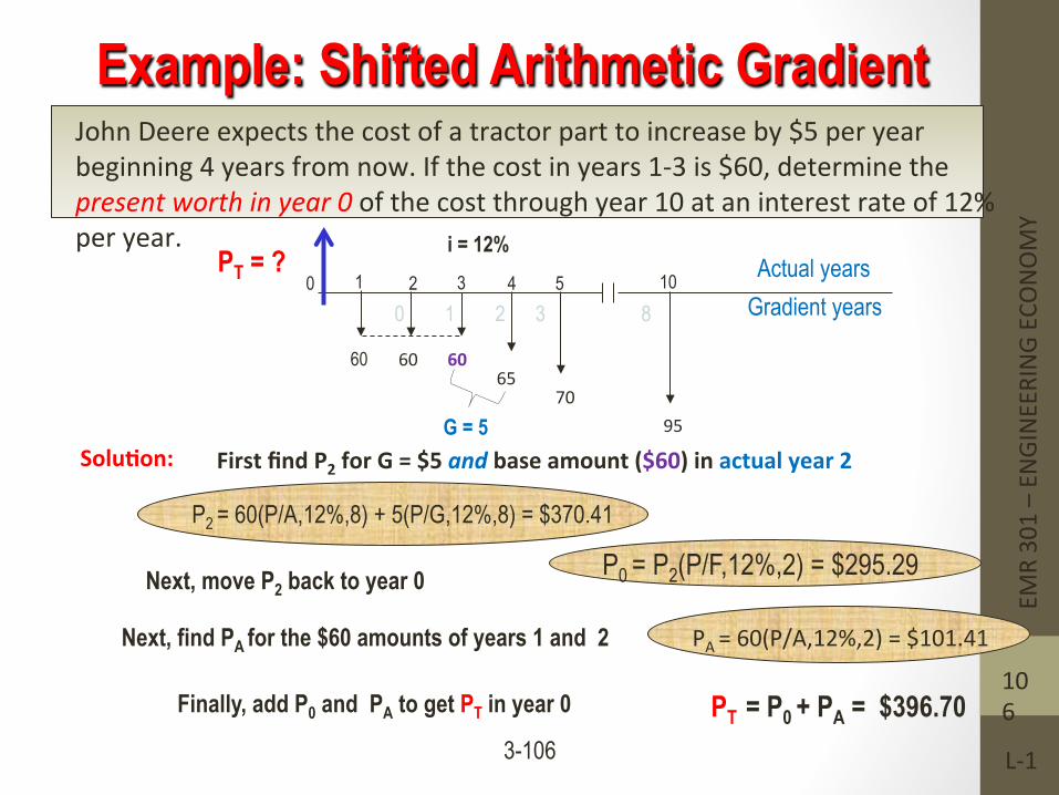
Example: Shifted Arithmetic Gradient

Solu=on:

John Deere expects the cost of a tractor part to increase by $5 per year beginning 4 years from now. If the cost in years 1-‐3 is $60, determine the present worth in year 0 of the cost through year 10 at an interest rate of 12% per year.

0

1 2 3 10 4 5

60 60 60 65

70 95

PT = ? i = 12%

First find P2 for G = $5 and base amount ($60) in actual year 2

P2 = 60(P/A,12%,8) + 5(P/G,12%,8) = $370.41

Next, move P2 back to year 0 P0 = P2(P/F,12%,2) = $295.29

Next, find PA for the $60 amounts of years 1 and 2 PA = 60(P/A,12%,2) = $101.41

Finally, add P0 and PA to get PT in year 0 PT = P0 + PA = $396.70

G = 5

0 1 2 3 8 Gradient years Actual years

EMR 301 – EN

GINEERING EC

ONOMY

L-‐1

106

Example 20

EMR 301 – EN

GINEERING EC

ONOMY

L-‐1

107

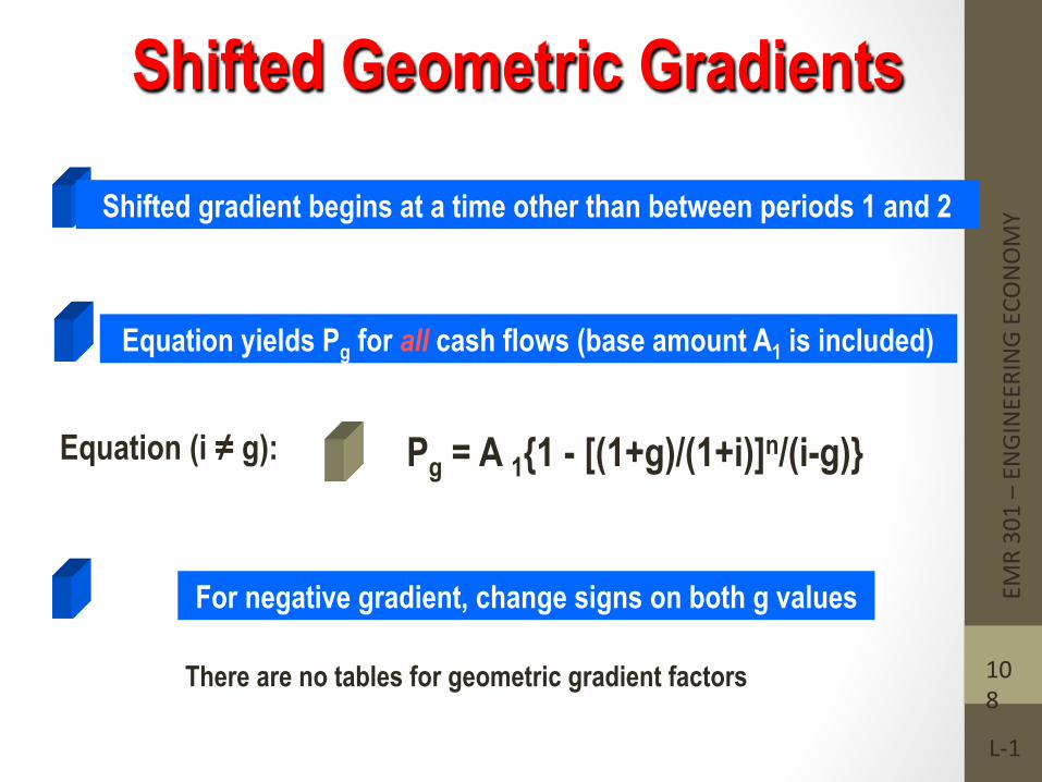
Shifted Geometric Gradients

Shifted gradient begins at a time other than between periods 1 and 2

Equation yields Pg for all cash flows (base amount A1 is included)

For negative gradient, change signs on both g values

Pg = A 1{1 - [(1+g)/(1+i)]n/(i-g)} Equation (i ≠ g):

There are no tables for geometric gradient factors

EMR 301 – EN

GINEERING EC

ONOMY

L-‐1

108

3-109

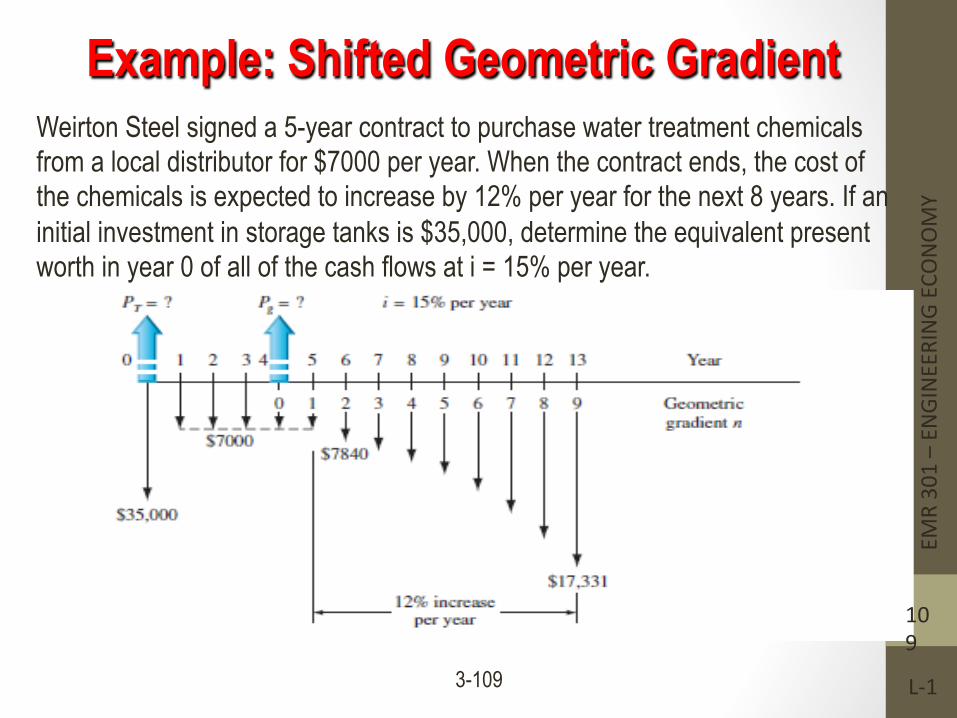
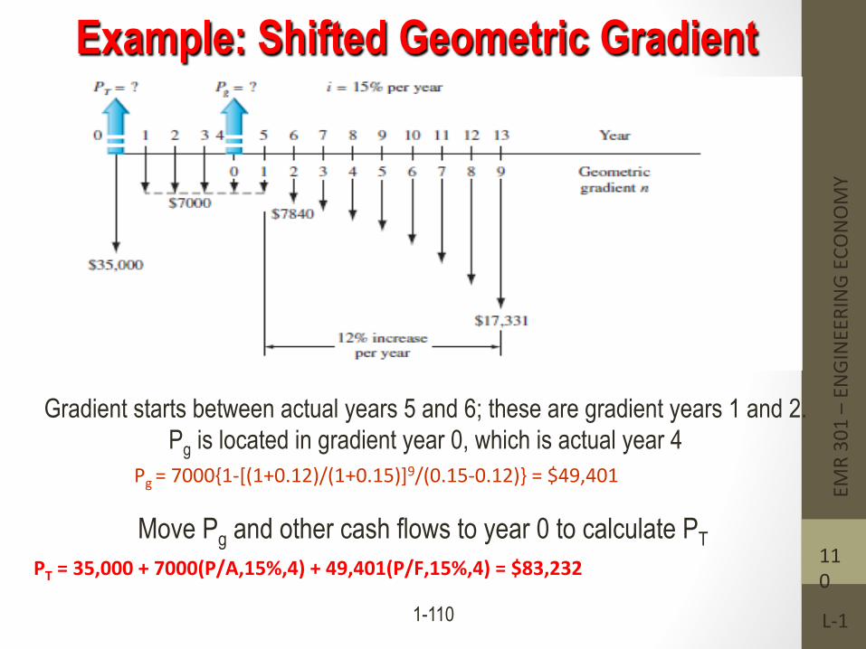
Example: Shifted Geometric Gradient Weirton Steel signed a 5-year contract to purchase water treatment chemicals from a local distributor for $7000 per year. When the contract ends, the cost of the chemicals is expected to increase by 12% per year for the next 8 years. If an initial investment in storage tanks is $35,000, determine the equivalent present worth in year 0 of all of the cash flows at i = 15% per year.

EMR 301 – EN

GINEERING EC

ONOMY

L-‐1

109

1-110

Example: Shifted Geometric Gradient

Gradient starts between actual years 5 and 6; these are gradient years 1 and 2. Pg is located in gradient year 0, which is actual year 4

Move Pg and other cash flows to year 0 to calculate PT PT = 35,000 + 7000(P/A,15%,4) + 49,401(P/F,15%,4) = $83,232

Pg = 7000{1-‐[(1+0.12)/(1+0.15)]9/(0.15-‐0.12)} = $49,401 EMR 301 – EN

GINEERING EC

ONOMY

L-‐1

110

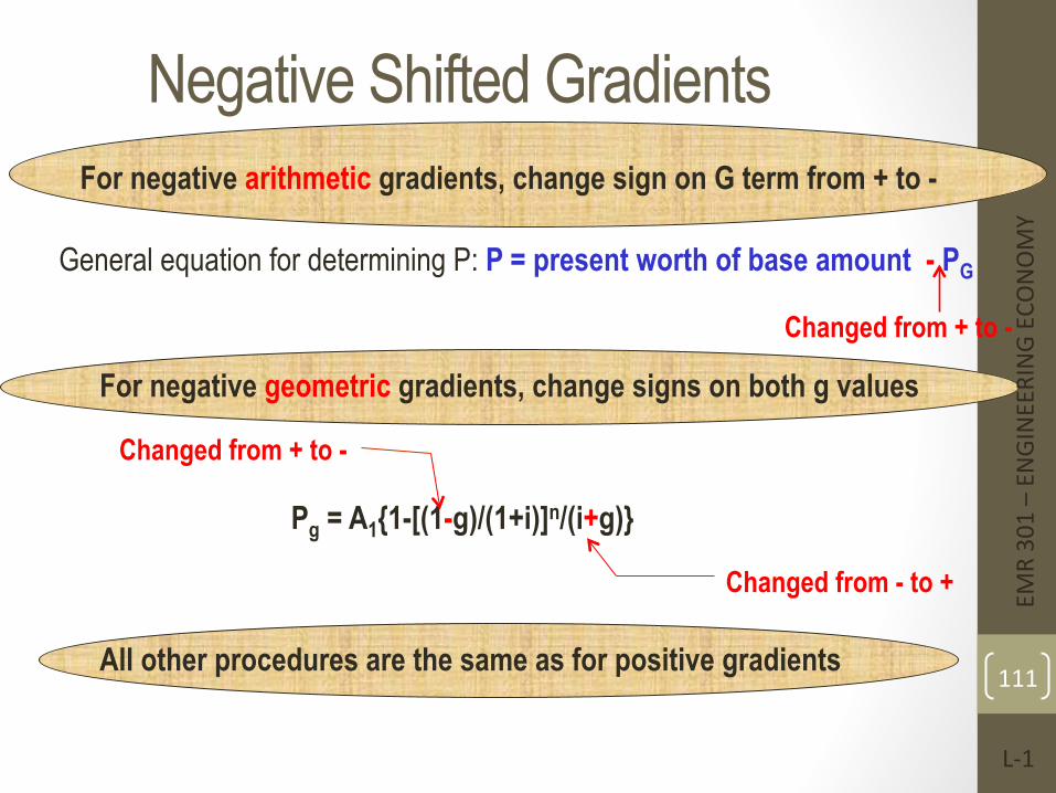
Negative Shifted Gradients For negative arithmetic gradients, change sign on G term from + to -

For negative geometric gradients, change signs on both g values

All other procedures are the same as for positive gradients

General equation for determining P: P = present worth of base amount - PG

Pg = A1{1-[(1-g)/(1+i)]n/(i+g)}

Changed from + to -

Changed from + to -

Changed from - to + EMR 301 – EN

GINEERING EC

ONOMY

L-‐1

111

Example: Negative Shifted Arithmetic Gradient

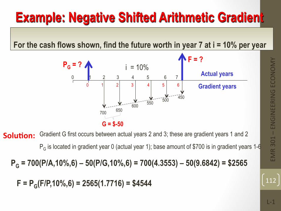
For the cash flows shown, find the future worth in year 7 at i = 10% per year F = ?

0 1 2 3 4 5 6 7

700 650

500 450 550 600

G = $-50 Gradient G first occurs between actual years 2 and 3; these are gradient years 1 and 2 Solu=on:

0 1 2 3 4 5 6

Actual years

Gradient years

PG is located in gradient year 0 (actual year 1); base amount of $700 is in gradient years 1-6

PG = 700(P/A,10%,6) – 50(P/G,10%,6) = 700(4.3553) – 50(9.6842) = $2565 F = PG(F/P,10%,6) = 2565(1.7716) = $4544

i = 10% PG = ?

EMR 301 – EN

GINEERING EC

ONOMY

L-‐1

112

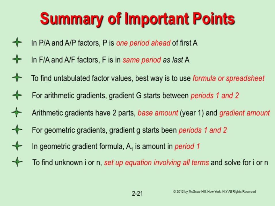
Summary of Important Points

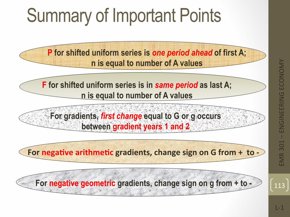
P for shifted uniform series is one period ahead of first A; n is equal to number of A values

F for shifted uniform series is in same period as last A; n is equal to number of A values

For gradients, first change equal to G or g occurs between gradient years 1 and 2

For nega=ve arithme=c gradients, change sign on G from + to -‐

For negative geometric gradients, change sign on g from + to -

EMR 301 – EN

GINEERING EC

ONOMY

L-‐1

113

engineeringeconomy - adnan menderes university · 2016-03-29 · engineering economy •...

Documents