Enhanced pair correlation functions in thetwo-dimensional Hubbard model

Takashi YanagisawaElectronics and Photonics Research Institute, National Institute of AdvancedIndustrial Science and Technology (AIST), Central 2, 1-1-1 Umezono,Tsukuba, Ibaraki 305-8568, JapanE-mail: t-yanagisawa@aist.go.jp

New Journal of Physics 15 (2013) 033012 (14pp)Received 11 October 2012Published 11 March 2013Online at http://www.njp.org/doi:10.1088/1367-2630/15/3/033012

Abstract. In this study we have computed the pair correlation functions in thetwo-dimensional Hubbard model using a quantum Monte Carlo method. Weemploy a new diagonalization algorithm in the quantum Monte Carlo methodwhich is free from the negative sign problem. We show that the d-wave pairingcorrelation function is indeed enhanced slightly for the positive on-site Coulombinteraction U when doping away from the half-filling. When the system sizebecomes large, the pair correlation function Pd increases for U > 0 comparedto the non-interacting case, while Pd is suppressed for U > 0 when the systemsize is small. The enhancement ratio Pd[U ]/Pd[U = 0] will give a criterion onthe existence of superconductivity. The ratio Pd[U ]/Pd[U = 0] increases almostlinearly ! L when the system size L " L is increased. This increase is a goodindication of the existence of a superconducting phase in the two-dimensionalHubbard model. There is, however, no enhancement of pair correlation functionsin the half-filled case, which indicates the absence of superconductivity withouthole doping.

Content from this work may be used under the terms of the Creative Commons Attribution-NonCommercial-ShareAlike 3.0 licence. Any further distribution of this work must maintain attribution to the author(s) and the title

of the work, journal citation and DOI.

New Journal of Physics 15 (2013) 0330121367-2630/13/033012+14$33.00 © IOP Publishing Ltd and Deutsche Physikalische Gesellschaft

2

Contents

1. Introduction 22. The Model and the wave function 3

2.1. Hamiltonian . . . . . . . . . . . . . . . . . . . . . . . . . . . . . . . . . . . . 32.2. Quantum Monte Carlo (QMC) method—Metropolis algorithm . . . . . . . . . 42.3. QMC method—diagonalization algorithm . . . . . . . . . . . . . . . . . . . . 5

3. Pair correlation functions 63.1. Comparison of the two methods . . . . . . . . . . . . . . . . . . . . . . . . . 73.2. Pair correlation in the two-dimensional Hubbard model . . . . . . . . . . . . . 8

4. Summary 11Acknowledgments 13References 13

1. Introduction

Strongly correlated electron systems have been studied intensively in relation to high-temperature superconductivity. High-temperature superconductors [1–4] are known to be atypical correlated electron system. In recent years, the mechanism of superconductivity in high-temperature superconductors has been extensively studied using various two-dimensional (2D)models of electronic interactions. Among them the 2D Hubbard model [5] is the simplest andmost fundamental model. This model has been studied intensively using numerical tools, suchas the quantum Monte Carlo (QMC) method [6–21] and the variational Monte Carlo (VMC)method [22–33].

The QMC method is a numerical method employed to simulate the behavior of correlatedelectron systems. It is well known, however, that there are significant issues associated with theapplication of the QMC method. The most important one is that the standard Metropolis (orheat bath) algorithm is associated with the negative sign problem. In past studies, workers haveinvestigated the possibility of eliminating the negative sign problem [16, 17, 19, 21].

In this paper, we adopt an optimization scheme which is based on the diagonalizationquantum Monte Carlo (QMD) method [21] (a bosonic version was developed in [34]), as wellas the Metropolis quantum Monte Carlo method (called the Metropolis QMC in this paper). Ingeneral, and as in this study, the ground-state wave function is defined as

! = e#" H!0, (1)

where H is the Hamiltonian and !0 is the initial one-particle state such as the Fermi sea. In theQMD method this wave function is written as a linear combination of the basis states, generatedusing the auxiliary field method based on the Hubbard–Stratonovich transformation, that is,

! =!

m

cm#m, (2)

where #m are basis functions. In this work, we have assumed a subspace with Nstates basiswave functions. From the variational principle, the coefficients {cm} are determined fromthe diagonalization of the Hamiltonian, to obtain the lowest energy state in the selected

New Journal of Physics 15 (2013) 033012 (http://www.njp.org/)

3

subspace {#m}. Once the cm coefficients are determined, the ground-state energy and otherquantities are calculated using this wave function. If the expectation values are not highlysensitive to the number of basis states, we can obtain the correct expectation values using anextrapolation in terms of the basis states in the limit Nstates $ %.

Whether the 2D Hubbard model can account for high-temperature superconductivity isan important question in the study of high-temperature superconductors. In correlated electronsystems, there is an interesting phenomenological correlation between the maximum Tc and thetransfer integral t :

kBTc & 0.1t/(m'/m), (3)

where m'/m indicates the mass enhancement factor and teff ( t/(m'/m) is the effectivetransfer integral. By adopting t ) 0.5 eV [35] and m'/m ) 5, this formula applies to high-Tc cuprates with Tc ) 100 K. As the electron becomes heavier, Tc is lowered (in accordancewith the lowering of Tc in the underdoped region). We can choose t ) 0.1 eV and m ' /m ) 2for iron pnictides to give Tc ) 50 K. This formula strongly suggests that high-temperaturesuperconductivity originates from the electron correlation and not from the electron–phononinteraction.

Most of the QMC method results do not support superconductivity, although the resultsof the VMC method with the Gutzwiller ansatz indicate the stable d-wave pairing statefor large U . The computations of the pair-field susceptibility suggest the existence of theKosterlitz–Thouless transition in the 2D Hubbard model indicating superconducting transitionin real three-dimensional systems [36, 37]. The perturbative and random phase approximation(RPA) calculations also support superconductivity with anisotropic pairing symmetry [38–42].In contrast, the pair correlation functions obtained by a QMC method [18] are extremelysuppressed for the intermediate values of U . This result suggests that superconductivityis impossible in the 2D Hubbard model. The objective of this paper is to compute paircorrelation functions and clarify this discrepancy using a new QMC method by employing thediagonalization scheme [21]. We show that the pair correlation function is indeed enhanced atdoping.

2. The Model and the wave function

2.1. Hamiltonian

The Hamiltonian is the Hubbard model containing on-site Coulomb repulsion and is written as

H = #!

i j$

ti j(c†i$ c j$ + h.c.) + U

!

j

n j*n j+, (4)

where c†j$ (c j$ ) is the creation (annihilation) operator of an electron with spin $ at the j th site

and n j$ = c†j$ c j$ . Note that ti j is the transfer energy between the sites i and j . ti j = t for the

nearest-neighbor bonds and ti j = #t , for the next-nearest-neighbor bonds. For all other casesti j = 0. U is the on-site Coulomb energy. The number of sites is N and the linear dimensionof the system is denoted as L , i.e. N = L2. The energy unit is given by t and the number ofelectrons is denoted as Ne.

New Journal of Physics 15 (2013) 033012 (http://www.njp.org/)

4

2.2. Quantum Monte Carlo (QMC) method—Metropolis algorithm

In a QMC simulation, the ground-state wave function is

! = e#" H!0, (5)

where !0 is the initial one-particle state represented by a Slater determinant. For large " , e#" H

will project out the ground state from !0. We write the Hamiltonian as H = K + V , where Kand V are the kinetic and interaction terms of the Hamiltonian in equation (4), respectively. Thewave function in equation (5) is written as

! = (e#%" (K +V ))m!0 - (e#%" K e#%" V )m!0 (6)

for " = %"m. Using the Hubbard–Stratonovich transformation [6, 43], we have

exp(#%"Uni*ni+) = 12

!

si =±1

exp(2asi(ni* # ni+) # 12

U%" (ni* + ni+)) (7)

for (tanh a)2 = tanh (%"U/4) or cosh (2a) = e%"U/2. The wave function is expressed as asummation of the one-particle Slater determinants over all the configurations of the auxiliaryfields s j = ±1. The exponential operator is expressed as [43]

(e#%" K e#%" V )m = 12Nm

!

{si (&)}

"

$

B$m(si(m))B$

m#1(si(m # 1)) · · · B$1 (si(1)), (8)

where we have defined

B$& ({si(&)}) = e#%" K$ e#V$ ({si (&)}) (9)

for

V$ ({si}) = 2a$!

i

si ni$ # 12

U%"!

i

ni$ , (10)

K$ = #!

i j

ti j(c†i$ c j$ + h.c.). (11)

The ground-state wave function is

! =!

n

cn#n, (12)

where #n is a Slater determinant corresponding to a configuration {si(&)} (i = 1, . . . , N ; & =1, . . . , m) of the auxiliary fields:

#n ="

$

B$m(si(m)) . . . B$

1 (si(1))!0

( #*n #+

n . (13)

The coefficients cn are constant real numbers: c1 = c2 = · · · . The initial state !0 is a one-particlestate. The matrix of V$ ({si}) is a diagonal matrix given as

V$ ({si}) = diag (2a$ s1 # U%"/2, . . . , 2a$ sN # U%"/2). (14)

New Journal of Physics 15 (2013) 033012 (http://www.njp.org/)

5

The matrix elements of K$ are

(K$ )i j =##t, i, j are nearest neighbors,0 otherwise. (15)

#$n is an N " N$ matrix given by the product of the matrices e#%" K$ , eV$ and !$

0 . The innerproduct is thereby calculated as a determinant [17],

.#$& #$

n / = det(#$†& #$

n ). (16)

The expectation value of the quantity Q is evaluated as

.Q/ =$

&n.#&Q#n/$&n.#&#n/

. (17)

P&n ( det(#$& #$

n ) det(##$& ##$

n ) can be regarded as the weighting factor to obtain the Monte Carlosamples. Since this quantity is not necessarily positive definite, the weighting factor should be|P&n|; the resulting relationship is

.Q$ / =!

&n

P&n.Q$ /&n/!

&n

P&n

(18)=

!

&n

|P&n|sign (P&n).Q$ /&n/!

&n

|P&n|sign (P&n),

where sign(a) = a/|a| and

.Q$ /&n = .#$& Q$#$

n /.#$

& #$n /

. (19)

This relation can be evaluated using a Monte Carlo procedure if an appropriate algorithm, suchas the Metropolis or heat bath method, is employed [43]. The summation can be evaluated usingappropriately defined Monte Carlo samples,

.Q$ / =1

nMC

$&n sign (P&n).Q$ /&n

1nMC

$mn sign (P&n)

, (20)

where nMC is the number of samples. The sign problem is an issue if the summation ofsign(P&n) vanishes within statistical errors. In this case, it is indeed impossible to obtain definiteexpectation values.

2.3. QMC method—diagonalization algorithm

Quantum Monte Carlo diagonalization (QMD) is a method for the evaluation of .Q$ / withoutthe negative sign problem. The configuration space of the probability 0 Pmn 0 in equation (20)is generally very strongly peaked. The sign problem lies in the distribution of Pmn in theconfiguration space. It is important to note that the distribution of the basis functions #m

(m = 1, 2, . . .) is uniform since cm are constant numbers: c1 = c2 = · · · . In the subspace {#m},selected from all configurations of auxiliary fields, the right-hand side of equation (17) can bedetermined. However, the large number of basis states required to obtain accurate expectation

New Journal of Physics 15 (2013) 033012 (http://www.njp.org/)

6

values is beyond the current storage capacity of computers. Thus, we use the variationalprinciple to obtain the expectation values.

From the variational principle,

.Q/ =$

mn cmcn.#m Q#n/$mn cmcn.#m#n/

, (21)

where cm (m = 1, 2, . . .) are variational parameters. In order to minimize the energy

E =$

mn cmcn.#m H#n/$mn cmcn.#m#n/

(22)

the equation ' E/'cn = 0 (n = 1, 2, . . .) is solved for,!

m

cm.#n H#m/ # E!

m

cm.#n#m/ = 0. (23)

If we set

Hmn = .#m H#n/, (24)

Amn = .#m#n/ (25)

the eigenequation is

Hu = E Au (26)

for u = (c1, c2, . . .)t. Since #m (m = 1, 2, . . .) are not necessarily orthogonal, A is not a diagonal

matrix. We diagonalize the Hamiltonian A#1 H and then calculate the expectation values ofcorrelation functions with the ground state eigenvector; in general A#1 H is not a symmetricmatrix.

In order to optimize the wave function, we must increase the number of basis states {#m}.This can be simply accomplished through random sampling. For systems of small sizes andsmall U , we can evaluate the expectation values from an extrapolation of the basis of randomlygenerated states. The number of basis states is about 2000 when the system size is small. Forsystems 8 " 8 and 10 " 10, the number of states is increased up to about 10 000.

In QMC simulations an extrapolation is performed to obtain the expectation values for theground-state wave function. The variance method has been proposed in variational and QMCsimulations, where the extrapolation is performed as a function of the variance. An advantageof the variance method is that linearity is expected in some cases [19, 44]:

.Q/ # Qexact ! v, (27)

where v denotes the variance defined as

v = .(H # .H/)2/.H/2

(28)

and Qexact is the expected exact value of the quantity Q.

3. Pair correlation functions

In this section, we present the results obtained by the QMC and QMD methods.

New Journal of Physics 15 (2013) 033012 (http://www.njp.org/)

7

(a) (b)

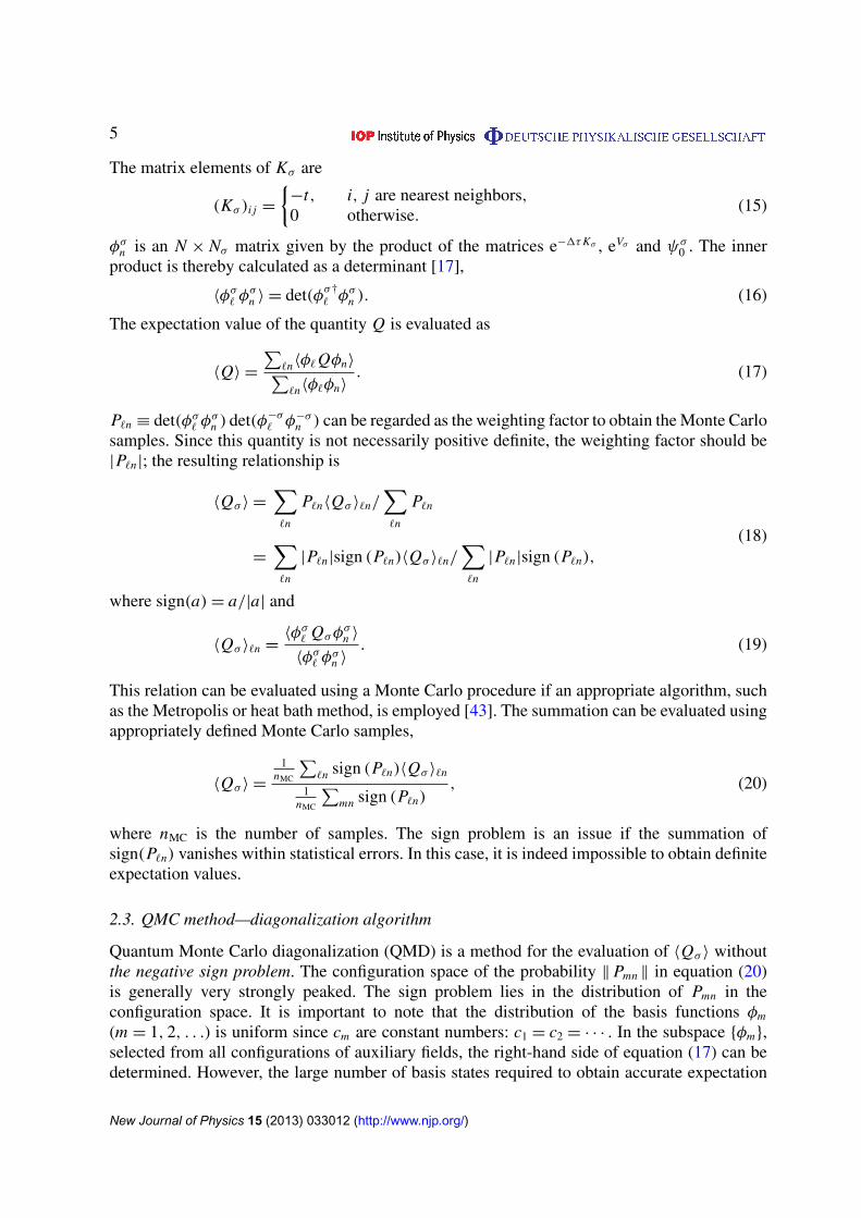
Figure 1. Pair correlation functions Dyy(&) and Dyx(&) for 4 " 3, U = 4 andNe = 10 obtained by the diagonalization QMC method (a) and the MetropolisQMC method (b). The squares are the exact results obtained by the exactdiagonalization method. In (a) the data fit using a straight line using the least-square method as the variance is reduced. We started with Nstates = 100 (the firstsolid circles) and then increase up to 2000.

3.1. Comparison of the two methods

The pair correlation function D() is defined by

D()(&) = .%†( (i + &)%)(i)/, (29)

where %((i), ( = x, y, denote the annihilation operators of the singlet electron pairs for thenearest-neighbor sites:

%((i) = ci+ci+(̂* # ci*ci+(̂+. (30)

Here (̂ is a unit vector in the ((= x, y)-direction. We consider the correlation function ofd-wave pairing:

Pd(&) = .%d(i + &)†%d(i)/, (31)

where

%d(i) = %x(i) + %#x(i) # %y(i) # %#y(i), (32)

i and i + & denote sites on the lattice.We show how the pair correlation function is evaluated in QMC methods. We show the

pair correlation functions Dyy and Dyx on the lattice 4 " 3 in figure 1. The boundary conditionis open in the four-site direction and is periodic in the other direction. An extrapolation isperformed as a function of 1/m in the QMC method with Metropolis algorithm and as afunction of the energy variance v in the QMD method with diagonalization. We keep %" asmall constant & 0.02–0.05 and increase " = %"m, where m is the division number m of thewave function ! in equation (5). In the Metropolis QMC method, we calculated averages over5 " 105 Monte Carlo steps. The exact values were obtained by using the exact diagonalizationmethod. The two methods give consistent results as shown in the figures. All the Dyy(&) and

New Journal of Physics 15 (2013) 033012 (http://www.njp.org/)

8

(a) (b)

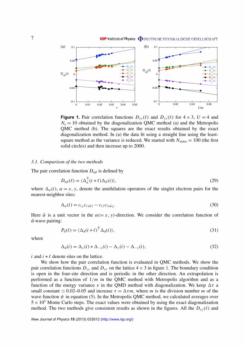
Figure 2. Pair correlation function Dyy(&) as a function of the energy variancev in (a) and 1/m in (b) for 30 " 2, U = 4 and Ne = 48. We used (a) thediagonalization QMC method and (b) the Metropolis QMC method. We set theopen boundary condition. From the top, & = (1, 0), (2, 0), (5, 0), (4, 0), (3, 0) and(6, 0).

Dyx(&) are suppressed on 4 " 3 when U is increased. In general, the pair correlation functionsare suppressed in small systems.

In figure 2, we show the inter-chain pair correlation function Dyy(&) as a function of1/m (b) and the energy variance (a) for the ladder model 30 " 2. We use the open boundarycondition. The boundary condition is not important for our purpose to check the consistencybetween QMC and QMD methods. The number of electrons is Ne = 48, and the strength of theCoulomb interaction is U = 4. %y(i) indicates the electron pair along the rung, and Dyy(&) isthe expectation value of the parallel movement of the pair along the ladder. The results obtainedby the two methods are in good agreement except for & = (1, 0) (nearest-neighbor correlation).

3.2. Pair correlation in the two-dimensional Hubbard model

We present the results for pair correlation in the 2D Hubbard model. In this section, we showthe results using the diagonalization QMC method because the Metropolis QMC method hasa negative sign problem. We first examine the 8 " 8 lattice. The Pd was estimated by anextrapolation as a function of the variance v, as shown in figure 3, where the computationswere carried out on an 8 " 8 lattice with U = 3, t , = #0.2 and Ne = 54. The extrapolation wassuccessfully performed for 8 " 8.

We consider the half-filled case with t , = 0; in this case the antiferromagnetic correlation isdominant over the superconductive pairing correlation and thus the pairing correlation functionis suppressed as the Coulomb repulsion U is increased. Figure 4(a) exhibits the d-wave pairingcorrelation function Pd on an 8 " 8 lattice as a function of the distance. The Pd is suppressed dueto the on-site Coulomb interaction, as expected. Its reduction is, however, not so considerablylarge compared to previous QMC studies [18] where the pairing correlation is almost annihilatedfor U = 4. We then turn to the case of less than half-filling. We show the results on 8 " 8 withelectron number Ne = 54. We show Pd as a function of the distance in figure 4(b) (Ne = 54). Inthe scale of this figure, Pd for U > 0 is almost the same as that of the non-interacting case, and is

New Journal of Physics 15 (2013) 033012 (http://www.njp.org/)

9

Figure 3. Pair correlation function Pd as a function of the energy variance v onan 8 " 8 lattice. U = 3, t , = #0.2 and the electron number is Ne = 54. We haveshown Pd(&) = .%d(i + &)†%(i)/ for & = (m, n) # i and i = (1, 1), where (m, n)are shown in the figure.

(a) (b)

Figure 4. Pair correlation function Pd as a function of the distance R = |&| on an8 " 8 lattice for (a) the half-filled case Ne = 64 and (b) Ne = 54. We set t , = 0.0and U = 0, 3 and 4 for (a) and t , = #0.2 and U = 0, 4 and 6 for (b). To liftthe degeneracy of electron configurations at the Fermi energy in the half-filledcase, we included a small staggered magnetization )10#4 in the initial wavefunction !0.

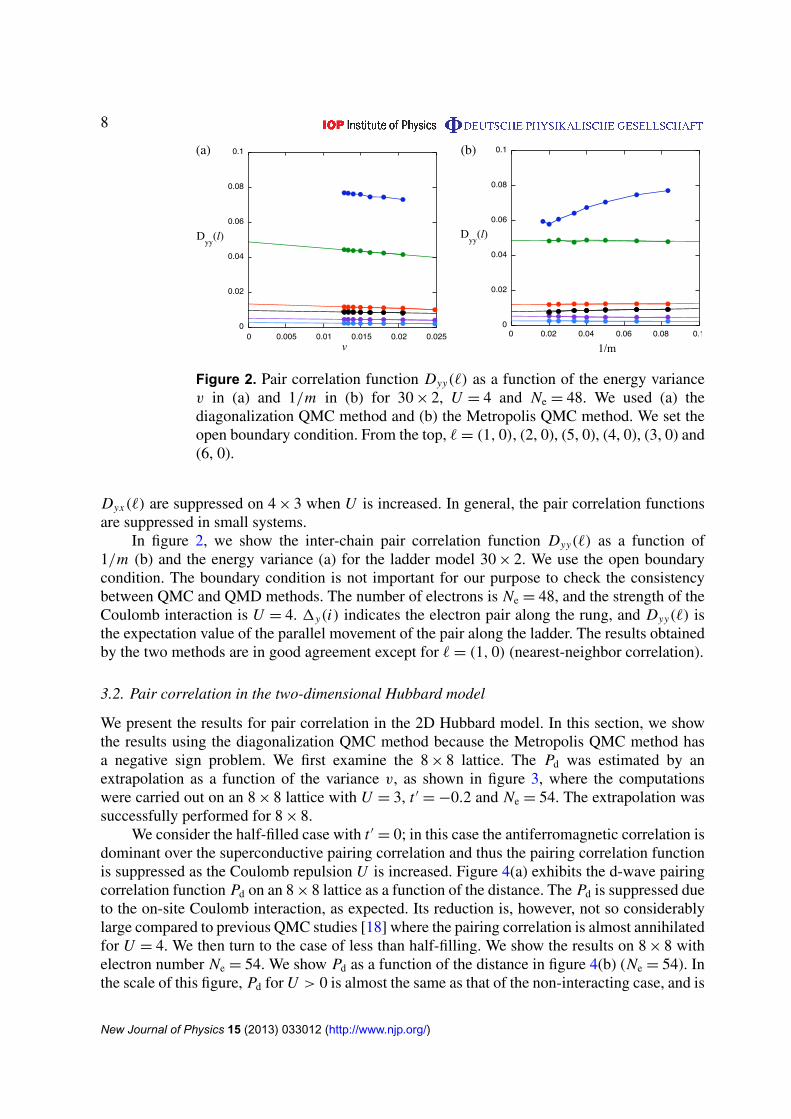
enhanced slightly for large U . Our results indicate that the pairing correlation is not suppressedand is indeed enhanced by the Coulomb interaction U , and its enhancement is very small.Figure 5 represents Pd as a function of U for Ne = 54, 50 and 64. We set t , = 0 for Ne = 50and t , = #0.2 for Ne = 54 so that we have the closed shell structure in the initial function. Inthe system of this size, the effect of the inclusion of t , 1= 0 is small. Figure 6 shows Pd on a

New Journal of Physics 15 (2013) 033012 (http://www.njp.org/)

10

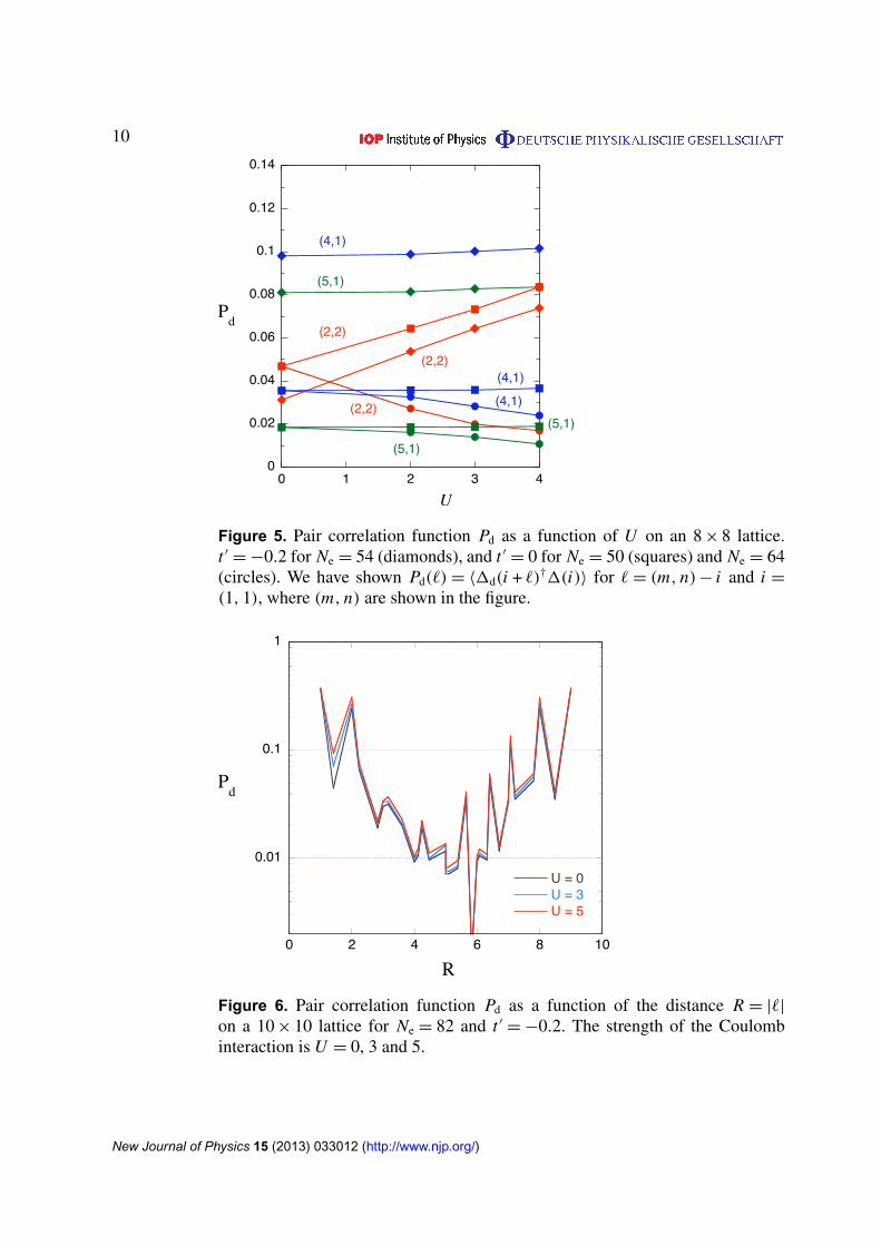
Figure 5. Pair correlation function Pd as a function of U on an 8 " 8 lattice.t , = #0.2 for Ne = 54 (diamonds), and t , = 0 for Ne = 50 (squares) and Ne = 64(circles). We have shown Pd(&) = .%d(i + &)†%(i)/ for & = (m, n) # i and i =(1, 1), where (m, n) are shown in the figure.

Figure 6. Pair correlation function Pd as a function of the distance R = |&|on a 10 " 10 lattice for Ne = 82 and t , = #0.2. The strength of the Coulombinteraction is U = 0, 3 and 5.

New Journal of Physics 15 (2013) 033012 (http://www.njp.org/)

11

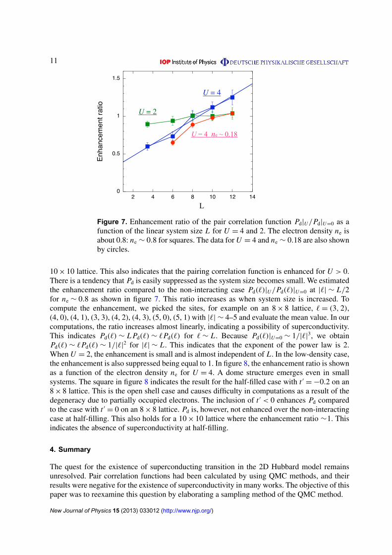
Figure 7. Enhancement ratio of the pair correlation function Pd|U/Pd|U=0 as afunction of the linear system size L for U = 4 and 2. The electron density ne isabout 0.8: ne ) 0.8 for squares. The data for U = 4 and ne ) 0.18 are also shownby circles.

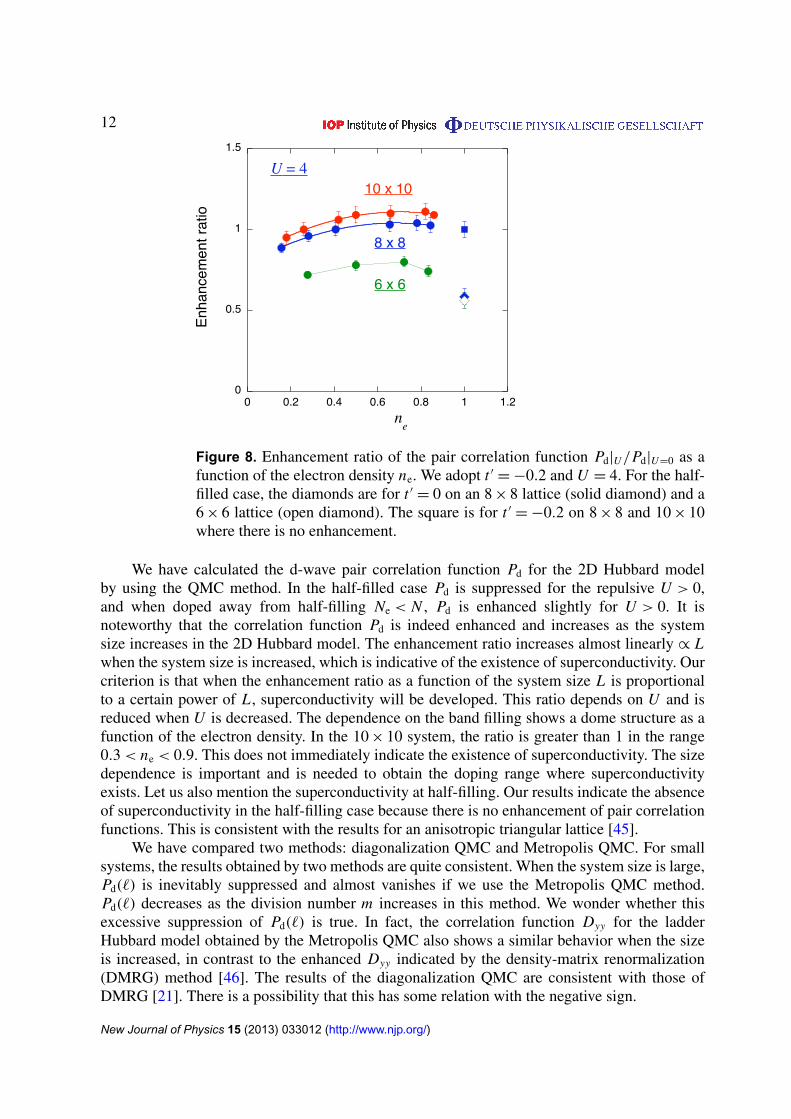
10 " 10 lattice. This also indicates that the pairing correlation function is enhanced for U > 0.There is a tendency that Pd is easily suppressed as the system size becomes small. We estimatedthe enhancement ratio compared to the non-interacting case Pd(&)|U/Pd(&)|U=0 at |&| ) L/2for ne ) 0.8 as shown in figure 7. This ratio increases as when system size is increased. Tocompute the enhancement, we picked the sites, for example on an 8 " 8 lattice, & = (3, 2),(4, 0), (4, 1), (3, 3), (4, 2), (4, 3), (5, 0), (5, 1) with |&| ) 4–5 and evaluate the mean value. In ourcomputations, the ratio increases almost linearly, indicating a possibility of superconductivity.This indicates Pd(&) ) L Pd(&) ) &Pd(&) for & ) L . Because Pd(&)|U=0 ) 1/|&|3, we obtainPd(&) ) &Pd(&) ) 1/|&|2 for |&| ) L . This indicates that the exponent of the power law is 2.When U = 2, the enhancement is small and is almost independent of L . In the low-density case,the enhancement is also suppressed being equal to 1. In figure 8, the enhancement ratio is shownas a function of the electron density ne for U = 4. A dome structure emerges even in smallsystems. The square in figure 8 indicates the result for the half-filled case with t , = #0.2 on an8 " 8 lattice. This is the open shell case and causes difficulty in computations as a result of thedegeneracy due to partially occupied electrons. The inclusion of t , < 0 enhances Pd comparedto the case with t , = 0 on an 8 " 8 lattice. Pd is, however, not enhanced over the non-interactingcase at half-filling. This also holds for a 10 " 10 lattice where the enhancement ratio )1. Thisindicates the absence of superconductivity at half-filling.

4. Summary

The quest for the existence of superconducting transition in the 2D Hubbard model remainsunresolved. Pair correlation functions had been calculated by using QMC methods, and theirresults were negative for the existence of superconductivity in many works. The objective of thispaper was to reexamine this question by elaborating a sampling method of the QMC method.

New Journal of Physics 15 (2013) 033012 (http://www.njp.org/)

12

Figure 8. Enhancement ratio of the pair correlation function Pd|U/Pd|U=0 as afunction of the electron density ne. We adopt t , = #0.2 and U = 4. For the half-filled case, the diamonds are for t , = 0 on an 8 " 8 lattice (solid diamond) and a6 " 6 lattice (open diamond). The square is for t , = #0.2 on 8 " 8 and 10 " 10where there is no enhancement.

We have calculated the d-wave pair correlation function Pd for the 2D Hubbard modelby using the QMC method. In the half-filled case Pd is suppressed for the repulsive U > 0,and when doped away from half-filling Ne < N , Pd is enhanced slightly for U > 0. It isnoteworthy that the correlation function Pd is indeed enhanced and increases as the systemsize increases in the 2D Hubbard model. The enhancement ratio increases almost linearly ! Lwhen the system size is increased, which is indicative of the existence of superconductivity. Ourcriterion is that when the enhancement ratio as a function of the system size L is proportionalto a certain power of L , superconductivity will be developed. This ratio depends on U and isreduced when U is decreased. The dependence on the band filling shows a dome structure as afunction of the electron density. In the 10 " 10 system, the ratio is greater than 1 in the range0.3 < ne < 0.9. This does not immediately indicate the existence of superconductivity. The sizedependence is important and is needed to obtain the doping range where superconductivityexists. Let us also mention the superconductivity at half-filling. Our results indicate the absenceof superconductivity in the half-filling case because there is no enhancement of pair correlationfunctions. This is consistent with the results for an anisotropic triangular lattice [45].

We have compared two methods: diagonalization QMC and Metropolis QMC. For smallsystems, the results obtained by two methods are quite consistent. When the system size is large,Pd(&) is inevitably suppressed and almost vanishes if we use the Metropolis QMC method.Pd(&) decreases as the division number m increases in this method. We wonder whether thisexcessive suppression of Pd(&) is true. In fact, the correlation function Dyy for the ladderHubbard model obtained by the Metropolis QMC also shows a similar behavior when the sizeis increased, in contrast to the enhanced Dyy indicated by the density-matrix renormalization(DMRG) method [46]. The results of the diagonalization QMC are consistent with those ofDMRG [21]. There is a possibility that this has some relation with the negative sign.

New Journal of Physics 15 (2013) 033012 (http://www.njp.org/)

13

Acknowledgments

We thank J Kondo, K Yamaji, I Hase and S Koikegami for helpful discussions. This work wassupported by a Grant-in-Aid for Scientific Research from the Ministry of Education, Culture,Sports, Science and Technology, Japan. This work was also supported by the CREST programof the Japan Science and Technology Agency (JST). Part of the numerical calculations wasperformed at the facilities in the Supercomputer Center of the Institute for Solid State Physics,University of Tokyo.

References

[1] Dagotto E 1994 Rev. Mod. Phys. 66 763[2] Scalapino D J 1990 Proc. on The Los Alamos Symp. High Temperature Superconductivity (1989) ed K S

Bedell, D Coffey, D E Deltzer, D Pines and J R Schrieffer (Redwood City: Addison-Wesley) p 314[3] Anderson P W 1997 The Theory of Superconductivity in the High-Tc Cuprates (Princeton, NJ: Princeton

University Press)[4] Moriya T and Ueda K 2000 Adv. Phys. 49 555[5] Hubbard J 1963 Proc. R. Soc. Lond. A 276 238[6] Hirsch J E 1983 Phys. Rev. Lett. 51 1900[7] Hirsch J E 1985 Phys. Rev. B 31 4403[8] Sorella S, Tosatti E, Baroni S, Car R and Parrinell M 1988 Int. J. Mod. Phys. B 2 993[9] White S R, Scalapino D J, Sugar R L, Loh E Y, Gubernatis J E and Scalettar R T 1989 Phys. Rev. B 40 506

[10] Imada M and Hatsugai Y 1989 J. Phys. Soc. Japan 58 3752[11] Sorella S, Baroni S, Car R and Parrinello M 1989 Europhys. Lett. 8 663[12] Loh E Y, Gubernatis J E, Scalettar R T, White S R, Scalapino D J and Sugar R L 1990 Phys. Rev. B 41 9301[13] Moreo A, Scalapino D J and Dagotto E 1991 Phys. Rev. B 56 11442[14] Furukawa N and Imada M 1992 J. Phys. Soc. Japan 61 3331[15] Moreo A 1992 Phys. Rev. B 45 5059[16] Fahy S and Hamann D R 1991 Phys. Rev. B 43 765[17] Zhang S, Carlson J and Gubernatis J E 1997 Phys. Rev. B 55 7464[18] Zhang S, Carlson J and Gubernatis J E 1997 Phys. Rev. Lett. 78 4486[19] Kashima T and Imada M 2001 J. Phys. Soc. Japan 70 2287[20] Yanagisawa T, Koike S and Yamaji K 1998 J. Phys. Soc. Japan 67 3867[21] Yanagisawa T 2007 Phys. Rev. B 75 224503[22] Yokoyama H and Shiba H 1987 J. Phys. Soc. Japan 56 1490

Yokoyama H and Shiba H 1987 J. Phys. Soc. Japan 56 3582[23] Gros C, Joynt R and Rice T M 1987 Phys. Rev. B 36 381[24] Nakanishi T, Yamaji K and Yanagisawa T 1997 J. Phys. Soc. Japan 66 294[25] Yamaji K, Yanagisawa T, Nakanishi T and Koike S 1998 Physica C 304 225

Yamaji K, Yanagisawa T, Nakanishi T and Koike S 2000 Physica B 284 415[26] Koike S, Yamaji K and Yanagisawa T 1999 J. Phys. Soc. Japan 68 1657

Koike S, Yamaji K and Yanagisawa T 2000 J. Phys. Soc. Japan 69 2199[27] Yanagisawa T, Koike S and Yamaji K 2001 Phys. Rev. B 64 184509[28] Yanagisawa T, Koike S and Yamaji K 2002 J. Phys.: Condens. Matter 14 21[29] Yanagisawa T, Miyazaki M, Koikegami S, Koike S and Yamaji K 2003 Phys. Rev. B 67 132408[30] Yanagisawa T, Miyazaki M and Yamaji K 2009 J. Phys. Soc. Japan 78 013706[31] Miyazaki M, Yamaji K and Yanagisawa T 2004 J. Phys. Soc. Japan 73 1643[32] Tocchio L T, Becca F and Gros C 2011 Phys. Rev. B 83 195138[33] Yokoyama H, Ogata M, Tanaka Y, Kobayashi K and Tsuchiura H 2013 J. Phys. Soc. Japan 82 014707

New Journal of Physics 15 (2013) 033012 (http://www.njp.org/)

14

[34] Mizusaki T, Honma M and Otsuka T 1986 Phys. Rev. C 53 2786[35] Feiner L F, Jefferson J H and Raimondi R 1996 Phys. Rev. B 53 8751[36] Maier T A, Jarrell M, Schulthess T C, Kent P R C and White J B 2005 Phys. Rev. Lett. 95 237001[37] Yanagisawa T 2010 J. Phys. Soc. Japan 79 063708[38] Scalapino D J, Loh E and Hirsch J E 1986 Phys. Rev. B 34 8190[39] Bickers N E, Scalapino D J and White S R 1989 Phys. Rev. Lett. 62 961[40] Hlubina R 1999 Phys. Rev. B 59 9600[41] Kondo J 2001 J. Phys. Soc. Japan 70 808[42] Yanagisawa T 2008 New J. Phys. 10 023014[43] Blankenbecler R, Scalapino D J and Sugar R L 1981 Phys. Rev. D 24 2278[44] Sorella S 2001 Phys. Rev. B 64 024512[45] Clay R T, Li H and Mazumdar S 2008 Phys. Rev. Lett. 101 166403[46] Noack R M, Bulut N, Scalapino D J and Zacher M G 1997 Phys. Rev. B 56 7162

New Journal of Physics 15 (2013) 033012 (http://www.njp.org/)