enhanced tcas ii cdti traffic sensor ... · enhanced tcas ii/cdti traffic sensor...
TRANSCRIPT

NASA Contractor Report 172445 1 _t 1
lqASA_CR-17244519850002619
L
Enhanced TCAS II/CDTI Traffic SensorDigitalSimulationModelAnd Program Description
Tsuyoshi Goka
CONTRACTNAS1-16135October 1984
__ " ",9_4.LANGLEY RESEARCH CENTEF_
LIBRARY, i_Ir_SA
HAMPTON, VIRGiNiA
https://ntrs.nasa.gov/search.jsp?R=19850002619 2020-05-24T01:29:30+00:00Z

!
i
!i!
Eiii
ii
[
P
I

EMTED:
_ -._,_ r.__ f s z'.-" 1
_=-u_'i...............0927=_ i _._.._o=.......... 2_ PAGE...... _,............._ ,.,'......,,.__,_,,", =, RPT_..........,,,,,_H-.:_.._,,=_-'_-"_"72445 _._..........i 2S ._T_= ...... _.............. o'I".-" zL-'--"_:.;t.-' i /'_ I-HL_L_, L.'i:_L.LH:_m:DIF i___'_''
.... " - ; _" - _- _- mF;,'-l-'-'-': .....IITTI:._..,,,-- _,_':'-:=n-"-''.,_,,,_.,__ TCP,S _.3"rnT:_., _ _-,_----.,,_,,r __. S_;;_L'_ d i '=;"t_] _,;mu.,dt ] O'ri ......... ,_,d ,-:-:-. n---.<,-,,,_.=t,_,,:,d.-..c._._-.Pt _.......... ""....... _w" TLSP.F,,:_] m.-.:-,.,,,
1.-11| ;-4-, ,,._.t, :- MiL_L;F:H.; . .
MU _[_o/riF u.=.,,
f;lHO_; /"Hi_ '_"_+-+-IL. , ,u, +-'_, ,-., , ,,,:, _,', "'_', +- ",', • ;_-" "'+-_- ......._. _-t_--'_l_)_.__. _--_,h. _1_-_i i _1 t! i
CO_,iPUTERi -'-_" " .......' ":_'................................................................ F,-'; ;t ;1- ; "-,_LL ! .._I !';L._LII ; i L_'_tl.-" "'1'I11 | FIr_I'IPI I ] L.HL
"INS " VERiF:: • / ,,-,__ ,_, .... I-UN..-:,;,_ .... _¢'P_MDIIT_DC, /•-_1 L_I_I .. i ± I-,'1-_
i._im;I.--I", ,,_..*,. i;i,H, .
_,_. O._'_-'_ _i,ui.-n;_.,u,,,...ode]u of ..--._,h-,_-.,-.,-,,-_TQqS c-.--'rr:T_..... "'--t:,., ,..,-_ ; S; M _ .-_: _.r_,a:_ _,_,..,.._ __, _c, _ _, i..[ dT i IL- .._._;_ll_,-t_-r _, ,_{_ -_.
chaioac:teristic: :- Tt._oez_hdrm:edTr,_-.fT,,_.',_)r Th_dt) ..=__t -"'-"-_Col.-, ,.._, ; }_;] t,_f}
......................... L.',-'II_.,L;_r_L;,_ t: LS, SJ 81" "rely
deve].-,,-,--.--:, ............ T:.+--.-,-;-+-.,.,_,-=+,--.--,_,.... t:ve .--,-h ....... ]t J iT';----- -_+ - - " _ ' ....b_[L:il =.-,_=.--:.._.-.e_.p__c--.i-,-4-'_-":............... --l- I "-.--_., r _--+lll_..'_._PI i._+-++....
-- -- --1_ 1_ _ Pe.P.P. ,- m Itliilj kl} ,_.t}le, mP, t-_iil-'-'-_-- ....... "; i .....i .......-relll,-_l:t. _L,L.'- tfal -+- .R.-..+.c-,--,i-.......... " ......_" ' " ......... :- ............... -_ ........... " .... S) FIU]_ i_i OF_ r u_hs,u,eS]u'-_'-lcr.uuu;es __ ,,.-_lddted +J:-.,++I_++++O, .-_...t=,,=,.,...-_ ._"
...................... -"_="-'-'--'.det_=" _+_d L..=_.._+b_l,t+eu......


NASA Contractor Report 172445
Enhanced TCAS II/CDTI Traffic SensorDigital Simulation ModelAnd Program Description
TsuyoshiGoka
Analytical MechanicsAssociates, Inc.Mountain View,California 94043
PreparedforLangleyResearchCenterNationalAeronauticsand SpaceAdministrationunder Contract NAS1-16135
National Aeronautics andSpace Administralon
Langley ResearchCenterHampton. Virginia 23665
October 1984


Foreword
This effort for developing enhanced TCAS II/CDTI
traffic sensor models was supported under NASA Contract
No. NASI-16135 by Langley Research Center, Hampton,
Virginia. The project technical monitor was Dr. Roland
L. Bowles of Langley Research Center. Technical dis-
cussions with Dr. Bowles and David H. Williams of NASA
Langley, and Joseph Fee of FAAHeadquarters are grate-
fully acknowledged.
i


ENHANCED TCAS II/CDTI TRAFFIC SENSOR
DIGITAL SIMULATION MODEL
AND
PROGRAM DESCRIPTION
Tsuyoshi Goka
Analytical Mechanics Associates, Inc.
Mountain View, California 94043
SUMMARY
The objectives of this project were to develop digital
simulation models of enhanced TCAS II/CDTI traffic sensors
based on actual or projected operational and performance
characteristics. Two enhanced traffic (or threat) alert and
collision avoidance systems were considered. The main focus
is a system based on the FAA/Bendix design which dates back
to the so-called Beacon Collision Avoidance System (BCAS)
concept. The other system is built by Dalmo Victor Division
of Textron's Bell Aerospace Co. based on the FAA/MIT active
BCAS concept.
Based on the engineering model, a digital simulation
program was developed in FORTRAN. The program contains an
executive with a seml-real time batch processing capability.
Thus, the simulation program can be interfaced with other
modules with a minimum requirement. The program is described
in detail.
The TCAS systems are not specifically intended for Cockpit
Display of Traffic Information (CDTI) applications. However,
these systems are sufficiently general to allow implementation of
CDTI functions within the real systems' constraints.
ii


TABLE OF CONTENTS
Page
I. INTRODUCTION ........................ i
II. ENHANCED TCAS II DESCRIPTION ........ . ....... 5
Background ......................... 5
Surveillance ........................ 8Estimation ......................... 18
Collision Avoidance Logic ................. 27Detection Logic ...................... 28
Resolution Advisory Selection ............... 39
III. BENDIX TCAS II SIMULATION PROGRAM DESCRIPTION ....... 47
Introduction ....................... 47
Executive Logic ...................... 49Sensor Module ....................... 59
Collision Avoidance Module ................. 76
IV. SIMULATION VALIDATION ................... 97
Simulation Set-Up ..................... 97BX TCAS Sensor Validation ................. 103
CAS Logic Validation .................... 139
V. CONCLUSIONS ........................ 149
APPENDIX A: Major Program Commons ................ 151
APPENDIX B: DV TCAS II Model Considerations ........... 161
REFERENCES - 167
iii


LIST OF FIGURES
Page
i. TCAS II Functional Elements ........... ..... 6
2. Range Track Regions at Various Own Altitudes ....... 13
3. TCAS Geometry ....................... 21
4. Schematic Diagram of Altitude Measurement Process ..... 25
5. Region Defining RA Range Test ............... 33
6. Region Defining RAAltitude Test ............. 35
7. Own Altitude Projection Model ............... 41
8. Resolution Advisory Selection Logic ............ 44
9. Enhanced BX TCAS II/CDTI Sensor Model Block Diagram .... 48
i0. BX TCAS Macro Flow Chart ................. 50
ii. BX TCAS Executive Logic .................. 53
12. BX TCAS Subroutine Structure ............... 54
13. Estimation Executive (ESTMTN) Flow Chart ...... . . . 65
14. Vertical Tracker Algorithm Macro Flow Chart ........ 68
15. Illustration of Level Switching Times and Altitude
Measurements . ...................... 69
16. Vertical CAS Logic Executive Macro Flow Chart ...... 75
17. ADVSEL Detailed Flow Chart ................ 84
18. Resolution Advisory Selection Subroutine Tree ...... 86
19. SELADVDetailed Flow Chart ................ 88
20. CHKPRJDetailedFlow Chart ................ @8
21. TKYVSL DetailedFlow Chart ................ 89
22. VSLINT DetailedFlow Chart ...... . ......... 9023. VSLTST DetailedFlow Chart ................ 90
24. ADVEVL DetailedFlow Chart ................ 9Z
25. TCAS SimulationValidationProgram ............. 98
26. SimplifiedCommand-ResponseBased Point MassAircraftDynamicModel .................. 100
27. SensorValidationPlotsfor Case (i) ........... 106
28. SensorValidationPlots for Case (2) ........... 113
iv

LIST OF FIGURES - Continued
Page
29. Own Lateral Dynamic Variables for Case (3) ......... 121
30. Sensor Validation Plots for Case (3) ............. 122
31. Sensor Validation Plots for Case (4) ............ 129
32. Definitions of Variables Associated with the Linear
Movements of Targets in the Range Dimension ........ 140
33. Schematic Diagram for Scenario (8) ............. 145
34. Comparison of VSL's at Different Altitudes ......... 147
E.I Flow Chart for the DV TCAS Sampler Logic .......... 164
V

LIST OF TABLES
Page
i. Operational Characteristics of Candidate TCAS/CDTISensor ........................... 7
2. FunctionalBreakdownof TCAS II with respecttoBearingAccuracy ...................... 8
3. Summaryof BX TCAS SurveillanceFunction .......... 17
4. BX TCAS HorizontalTrackere and 8 Gain Values ....... 24
5. SensitivitySelectionAltitudeSchedule .......... 29
6. TA Range Test ....................... 29
7. TAAltitude Test ...................... 30
8. TA ThresholdValues .................... 31
9. RA Range Test ....................... 3334i0. VerticalMiss-DistanceComputation.............
ii. RA ThresholdValues .................... 37
3812. Summaryof Threat DetectionTests..............
4213. Climb or DescendSense Selection..............
4314. TCAS ResolutionAdvisories.................
15. Vertical ResolutionAdvisoryBit Patterns ......... 46
16. List of External Input ................... 51
17. Short FunctionalDescriptionof Major Subroutines ..... 55
18. Explanationof Program Common Contents ........... 576D19. Own Related Computation(TRKOWN) ..............
20. DETECT SubroutineComputationalSteps ........... 78
21. CASSTS SubroutineComputationalSteps ........... 81
22. FunctionalEvaluationof LADSTS .............. 82
23. SELSNS SubroutineComputationalSteps ........... 86
24. VMDP ComputationTable .................. 91
25. CAS File VariablesStored by the PackingRoutines ..... 94
26. CAS Output VariableMap .................. 93
27. DynamicEquationsfor Point Mass AircraftDynamicModel (7-State)....................... i01
28. TrafficInitialization................... 102
29. CAS Logic ValidationCases ................. 142
vi

LIST OF TABLES - Continued
Page
A.I /OWNTFL/ and /ITRGT/ Common Definitions .......... 152
A.2 /BNDXFL/ Common Definitions ................ 153
A.3 /ZTRKFL/ and /ZWRKVR/ Common Definitions ......... 154
A.4 /WORKVR/ Common Definitions ................ 155
A.5 /CASFIL/ Common Definitions ................ 157
A.6 /CWRKVR/ and /CWRKV2/ Common Definitions ......... 158
A.7 /CASPAR/ Common Definitions ................ 159
B.I Probability of DV TCAS Surveillance Data Drop-out ..... 163
vii

LIST OF ACRONYMSAND ABBREVIATIONS
AGL Above Ground Level
ATC Air Traffic Control
ATCRBS Air Trafflc Control Radar Beacon System
BCAS Beacon Collision Avoidance System
CAS Collision Avoidance System
CDTI Cockpit Display of Traffic Information
CPA Closest Point of Approach
EFR Electronic Flight Rules
EHSI Electronic Horizontal Situation Indicator
FAA Federal Aviation Administration
INS Inertial Navigation System
LOT Level Occupancy Time
LST Level Switching Time
MFD Multi-Function Display
MSL Mean Sea Level
Mode A An ATCRBS reply format with aircraft identity
Mode C An ATCRBS reply format containing an altitude report
Mode S New Selectable data formats used by a Mode S transponder
MOPS Minimum Operational Performance Standards
NASA National Aeronautics and Space Administration
NED north-east-down (a standard coordinate system)
PWI Proximity (or Pilot) Warning Indicator
RF Radio Frequency
TCAS Traffic (or Threat) Alert and Collision Avoidance System
VFR Visual Flight Rules
viii


I
INTRODUCTION
NASA Langley Research Center is pursuing a research _effort con-
cerning the Cockpit Display of Traffic Information (CDTI) concept. The
CDTI is a device which presents information to the pilot and crew de-
picting the status of surrounding traffic including position and velo-
City states. The general CDTI avionics consists of a "traffic sensor",
a pilot interface unit, a CDTI signal/data processor, and a display
unit.
The pilot interface unit can be a simple on/off switch, a shared
keyboard, or an elaborate touch sensitive screen. The CDTI signal/data
processor can be a digital data link between the traffic sensor and
signal operator or a bona fide computing module performing data edit-
ing, traffic selection or similar functions. The computational module
may be imbedded, for example, in a navigation computer. A cathode ray
tube (CRT) or a flat panel plasma display unit seems to be the most
suitable display medium.
Again, this system could be dedicated, shared, or imbedded in with
other functions. It would most logically be included in an Electronic
Horizontal Situation Indicator (EHSI) or a Multi-Function Display's (MFD)
symbology. It is also possible that the CDTI display could be included
in a general "Air Traffic Control" display unit in a futuristic environ-
ment if one were to extrapolate the current digital avionics and up-and-
down link communication technology and the centralized and automated
ground control philosophy.
The CDTI functions include both passive (monitoring) and active
roles. The latter is sometimes referred to as ElectronicsFlight Rules
(EFR) as compared to the VFR or IFR control environment. Some of the
envisioned CDTI functions are listed below:

TrafficMonitoringRoles:
GeneralTrafficMonitoring
LongitudinalSeparationof Arrivals
IndependentParallelApproaches
OceanicRoute Separation
ActiveControlRoles:
ArrivalMerging
Arrival In-trallSpacingControl
EnroutePassing and Crossing
SevereWeatherAvoidance
As can be seen from the above list of functions, the mainutility of
the CDTI is to provide the pilot with a strategic information base which
allows him to make appropriate decisions. This is counter to other
avionics which have well defined tactical functions. (For example, the
MLS (Microwave Landing Syst_n) provides deviation signals from reference
for the pilot to nullify.) This means that the CDTI utility can not be
measured by quantitative attributes such as accuracy or sampling frequency
alone. This utility also involves the question of how the pilot uses
the information b@se; i.e., the human factors aspect.
Therefore, various CDTI issues must be resolved via active, pilot-
in-the-loop simulation studies. This points out the importance of de-
veloping a realistic _imulation facility to reflect a "real" full work-
load flight environment. This issue is not limited to the "traffic sen-
sor" modeling, but it _cludes a host of other simulation elements.
Because there seems to be no official impetus to develop a CDTI
traffic sensor per se at this time, an experimental sensor simulation
model must be developed based on related systems which are currently being
developed. The FAA developed Traffic Alert and Collision Avoidance System
(TCAS) comes closest to fulfilling various CDTI research needs.
2

TCAS is strictlyan airbornesystemwhich providesthe aircraft
separationprotectioninformationindependentof the groundATC system.
The FAA plans call for develop_g two types of TCAS - TCAS I and TCAS
II. Within each category,a certain latitudein capabilityis allowed
to satisfya wide spectrumof user requirements.
The enhancedTCAS II which is capableof obtainingrelativebearing
measurementsbetween the protected(Own) and surroundingaircraft (Target)
may be able to supportCDTI applications. The enhancedTCAS II is capable
of range and bearing (in additlonto the encodedaltltude)measurements
with a medium degree of accuracy to the extent that a more sophisticated
CDTI type displayor horizontalcollisionavoidancelogic may be supported.
There are two designs in this enhancedTCAS II category. One design,de-
veloped by MIT/DalmoVictor (DV TCAS), is based on the so-calledactive
Beacon CollisionAvoidanceSystem (BCAS). The other, developedbyBendix
(BX TCAS), is based on the so-calledfull BCAS concept.
In supportof the NASA LangleyCDTI researcheffort,a comprehensive
digital simulationmodel of the enhancedTCAS II based on the Bendix design
(BX TCAS) has been develbped. The reasonsbehind this choice are two-
fold. First,because of its inherentaccuracy,other TCAS based traffic
sensorscan be "emulated"by degradingthe BX T_S model performance.
Second,the versatilityof the TCAS processorprovidesa certainmodification
latitudesuitablefor CDTI applications.
This report is a companionto our report entitled"Analysisof Estima-
tion Algorithmsfor CDTI and CAS Applications[i]",which studiesthe sensor
accuracyanalysiswith respectto CAS logic and CDTI applications. This
report is organizedas follows. Chapter II providesan engineeringdescrip-
tion of the BX TCAS II system. ChapterIII providesa detaileddescription
of the supportingsimulationprograms. ChapterIV provides the Input/
Output requirementsfor the BX TCAS module. ChapterV discussesa set of
simulationvalidationcases. The validationcases were selectedfrom
the draft TCAS II MinimumOperatingPerformanceStandardsby the
3

RTCA SC-147 [2], Chapter V provides the conclusions. Appendix A lists
all the major commons used in the simulation program. Appendix B dis-
cusses the major functional departure for the Dalmo Victor TCAS II (DV
TCAS) design. It also includes a set of program modifications in order
to incorporate system peculiarities.
4

II
ENHANCED TCAS II DESCRIPTION
Background
TCAS provides informationfor safe aircraftseparationindependentof
the ground ATC sensors. Except for TCAS I (whichoperateson a passive
listeningmode in prlnciple),TCAS containsan (active)transmitteras well
as an ICAO approvedModel S transponder. Target relativepositionalmeasure-
ments are acquiredby means of radio frequency(RF) transactionsof 1030 MHz
interrogationtransmissionand 1090 MHz reply reception. (Note that the RF
formatsare compatiblewith the currentATC surveillancesystem requirements.)
Fourmajor submodules-- surveillance,state estimation,collision
avoidancelogic, and pilot warningand display-- furtherprocessthe RF
transactionsto satisfythe aircraftseparationrequirements. Figure 1 depicts
the functionalbreak'downof these four submodules*. Each of these submodules
will be discussedin subsequentsections.
A relative bearing measurement capability is not a requirement for minimum
TCAS II; the bearing capability constitutes the "enhancement". Enhanced TCAS II
is capable of range and bearing (in addition to the encoded altitude) measure-
ments with a medium degree of accuracy to the extent that a more sophisticated
CDTI type display or horizontal collision avoidance logic may be supported.
Two systems in this category are at various stages of development or
testing. _F1ight evaluation of the DV TCAS will begin shortly in scheduled
operational environment [3]. The TCAS generated advisories will be displayed
to the flight crew. The BX TCAS engineering unit is currently undergoing an
* It is noted that the time sequence of events over one TCAS cycle is
closely correlated with the top to bottom items, i.e., the collision
avoidance logic requires the latest available state estimates which,
in turn, depend on the latest available surveillance data.

surveillanceMeasrent sCorrelation ATCRBS
_ Horizontal i
Estimation
Vertical I
Threat detection
Collision Avoidance Threat resolution
Maneuver Coordination
Own Display
i _ Traffic advisory
D_o_o__oe_°"°_I_o.,o_u_on_,v_.,o_
Figure i. TCAS II Functional Elements.

extensive flight test evaluation [4]. Table i shows the over-all performance
and operational characteristics of these two systems• Table 2 shows the
consensus of engineering opinion indicating the TCAS functional breakdown
and bearing accuracy•
In subsequent sections, functional descriptions of the four submodules
are given based on the BX TCAS design• It seems to be more suitable than
the DV TCAS for the CDTI applications in terms of coverage volume, accuracy,
and versatility• The material presented here is condensed, mainly from
the draft TCAS II MOPS and Bendix reports [1,5,6,7,8].
Table i. Operational Characteristics of Candidate TCAS CDTI Sensors
DV TCAS II BX TCAS II..... ,....... i . . |
Mode Base • Aircraft based • Aircraft based
• Independent of ground • Independent of ground
Coordinate • Aircraft .fixed • Aircraft fixed
System • Aircraft Body Axes • NED Local Level
Coverage • Within I0 nmi (max) of • Within 25 nmi (max) ofOwn Own
Accuracy • range = I00 ft rms • range = I00 ft rms
• bearing= 6-8 deg rms • bearing = 2 deg rms• altitude = I00 ft reso- • altitude = i00 ft reso-
lution lutlon
Sampling • I sec • I-8 sec (variable)Rate • reliability = f(range) • reliability high
Comments • u8 tracker in r-8 axes • u8 tracker in x-y axis
• LO tracker (altitude) . LO tracker (altitude)• Estimate not stabilized . Estimate stabilized with
with respect to Own respect to Own attitudeattitude i.e., #, 8, _ are avail-
. Global protection able within the TCAS• Medium traffic density processor
• Global protection
• High traffic density

Table 2. Functional Breakdown of TCAS IIwith Respect to Bearing Accuracy
, , , , , , ,
Bearing Accuracy Function
(deg)L
o Vertical Resolution4-8
(bearing modified)Enhanced
o PWI or CDTITCAS II
o Horizontal and
0.6 - 2 Vertical Resolution
o CDTI
Surveillance
The surveillance process begins by the TCAS transmitting 1030 MHz
interrogation signals and by receiving 1090 MHz replies from nearby
transponders (Mode A, ATCRBS or Mode S) or by listening for Mode S squitter
or alr-to-ground transmission signals at 1090 }_z. The position measure-
ments are then computed by the internal signal processor as follows:
(a) range - by the time duration between the interrogation and
the corresponding reply reception, accounting for the trans-ponder delay;
(b) bearing - by computing the angle-of-arrival from the phasedistribution among several antennas; and,
(c) altitude - by decoding the Mode C altitude code contained in
the reply. (For a Mode A only target, this will be non-existent.)
The surveillance characteristics of the BX TCAS are somewhat similar
to that of the ground based Mode S beacon sensor. Because a large number
of transmitters in a small local will cause interference resulting in
synchronous garble, fruit or false squitter detection, there are three
8

techniques (_n addition to the mono-pulse technique) to overcome the high
density problem. One is the interrogation antenna directivity; the second
is the so-called "whisper/shout" signal power level sequencing; and the
•third is the interrogation reschedullng if a reply is missed or garbled.
The antenna beam width is 22 1/2 deg; however, by_ repeating the trans-
mission four times and each time sliding the beam center by 5.625 deg, the
effective beam width becomes 5.625 deg. The beam pointing and rescheduling
as well as several levels of whlsper/shout power sequencing are controlled
by internal digital processors based on the internal track file, Own
aircraft's orientation, and the ATCRBS/Mode S transponder mix. The task
is facilitated by the fact that the beam is "stabilized" with respect to
roll, pitch and yaw attitude angles.
Target Track Establishment The function of establishing the target
track consists of two subfunctions: relative position measurement and the
associated target correlation. The position measurement refers to the
actual RF activities between Own's transmltter/receiver and Target's trans-
ponders and the subsequent signal processing to extract the position measure-
ment. The correlation process (also referred to as the track acquisition or
establishment) establishes the correspondence between a set of measurements
and a particular tracked aircraft.
It is simple to track Mode S equipped aircraft because of the uniquely
assigned discrete address in the reply format (which is also stored in the
TCAS unit). The task of correlating between the measurements and the tracked
aircraft is not as simple if the target is Mode C or Mode A equipped. Also,
for the narrow beam system (BX TCAS), the correlation process is simpler
than for the omni-directional or wide angle system, because the number of
replies corresponding to an interrogation is generally much smaller. However,
even the narrow beam width and the rescheduling capability present problems
if two or more aircraft are clustered in close proximity.
A "gating" technique is used for the purpose of separating targets. If
the currentmeasurement falls within certain threshold values (which define
the gate) of the predicted value of an aircraft in the track file, then the
m_
9

measurement is assigned to that aircraft, and the corresponding track file
is updated. If the measurement does not correspond consistently (5 - I0 sec)
within a gate to any existing aircraft in the track file, then a new track
file is started for that set of measurements. Conversely, if none of the
measurements consistently correspond to an aircraft in the file, then that
aircraft is judged outside the beam reach, and hence, it is deleted from
the track file.
The state estimates play an important role in computing the prediction
since the last valid measurement time. The estimation algorithms used for
this purpose are classical simple alpha-beta trackers. Accuracy is not too
critical because the threshold values are sufficiently large to account for
estimation errors.
There are still problems with the TCAS system proto-type which is
currently being flight tested. Track establishment of an "image target"
due to multi-path of the real target is one of the remaining major problems.
Coverage Volume The Own protected airspace provided by the system is
physically limited because of transmitter power output and/or receiver
reception sensitivity limitations. Also, the beam pattern due to the antenna
configuration comes into play, especially for the vertical coverage. The
maximum beam reach is estimated to be 35 nml; this is at the highest sen-
sitivity level. Within this distance, the 1030 _z transmission signals
can be distinguished from the ambient RF noise with a certain reliability.
The vertical limitation is due to the elevation beam shape. The top
mounted antenna assembly is designed to provide coverage of approximately
five (5) deg below and 23 deg above the antenna plane. The system may or
may not include a similar antenna assembly located at the bottom of the
fuselage.
To limit unnecessary RF activity, especially in a high traffic density
area, the BX TCAS relies on an "artificial" boundary generated by the beam
I0

control microprocessor. The volume is dynamically computed and is defined
by the relative range and relative altitude. In case of a Mode A transponder,
the range defines the volume. Furthermore, the volume is subdivided into
two regions - "acquisition" and "track".
The acquisition region is provided mathematically by
Ar ! Arac q, and IAhl ! Ahac q • (i)
Here Ar is the (.acquisition)range threshold (nominally 17 nmi for Mode Aacq
and Mode C transponders and 25 nml for Mode S transponders), and Ahacq is
the altitude threshold (nominally 6,000 ft but ignored for Mode A transponder).
The track region is provided mathematlcally by
• Ar ! Artr k, and IAhl ! Ahtr k • (2)
Here Artr k is the (track) range threshold which is computed dynamically,
and Ahtr k is the altitude threshold given by
Ahtr k = 3750 + Izl • 45 (ft) . (3)
The quantity Artr k is determined based on the relative bearing as well as
Own ground speed and altitude. The equation defining for this term is
given by
Artrk = Max{Arllm, (V0 cosAb + VMax) T + Ars} (_)
Here,
V0 = Own ground speed, in kt,
T = "closure" time constant = 1/80 hr = 45 sec, and
Ab = relative bearing with respect to Own's body axes-i
= tan (AYB/AX B)
Ar = 1.65 nmi.s
Arli m and VMax are computed based on Own altitude Zo (ft), according to
ii

^
I 5 nmi, if z0 _ i0,000 ftArlim = (5)
10 nmi, otherwise
and
• ( 250 kt, _0 ! 3,000 ft.
_tax I _0/20 + 100 kt, 3,000 < _0 ! I0,000 ft. (6)600 kt, Zo _ 10,000 ft.
Figure 2 shows the track regions corresponding to three Own ground speeds
at three Own altitude levels. It is noted that the Own forward direction
is given a heavier protection weight.
Interrogation Schedule LoBic The antenna pointing controller module
schedules the interrogation and reception timing (i.e., surveillance
scheduling). The surveillance operation depends on two factors. One is
the transponder type - Mode C or Mode S. The other is the operational
mode - search/acquisltion or track. The antenna dwell at a given azimuth
angle is divided into one passive and three active processes. The active
ones include: (m) ATCRBS transmissions to search for ne___wwtargets(targets
which are not in the internal track file); (b) ATCRBS transmissions for
tracking existing targets (in the internal track file); and (c) Mode S
transmissions for tracking Mode S equipped targets. The passive process
consists of possibly listening for Mode S squirters or Mode S replies to
ground interrogations.
The time interval between ATCRBS search interrogations, At , isS
computed according to the formula:
Ats = min 16 sec, VMa x _'V_sAb (7)
where the variables have been previously defined.
The ATCRBS track interrogations are made for those targets lying
inside the track volume satisfying Eq. (2). The ATCRBS track interrogation
time interval_ AtT, is computed based on the predicted relative motion of
12

10
I
i 15 nml-15 0 Own
-15-
(a) V0 = 150 kt
Figure 2. Range Track Regions .
at Various Own Altitudes.
13

• -15-
(b) V0 = 300 kt
Figure 2. - Continued
14

nml15'
I J
-15 0 Own 15nml
-15.
(c) V0 = 600 kt
Figure 2. - Continued
15

the target. It is given hy the formula
AtT = Max {i sec, rain {tl, t2, t3, 8 sec} }. (8)
Here,
tI = the number of seconds it will take the targetto move 3 deg in bearing,
t2 = the number of seconds it will take the targetto move I000 ft in range, and
t3 = the number of seconds it will take the targetto move 250 ft in altitude.
Interrogation scheduling logic for targets with Mode A transponders
is presumed to be similar to the ATCRBS interrogations. However, the
target altitude logic would be ignored. Furthermore, if Own altitude is
too high compared to the FAA's altitude encoding transponder requirements,
then the Mode A targets can safely be ignored.
The interrogation scheduling logic for targets with Mode S transponders
are similar to the ATCRBS transponder case. When a new Mode S target is
detected by squirter listening, it is interrogated. If it is within the
acquisition range, Aracq, a track is initiated. Mode S equipped targets
inside the track volume are interrogated at the same rates as if they were
ATCRBS targets. Those targets which are outside of the volume but within
Ar of Own are tracked at a regular interval of eight (8) sec.acq
If a target (either ATCRBS or Mode S equipeed) is closer than 6000 ft
or if it has been declared a preliminary threat by the threat direction logic,
the target track update rate is one (i) sec.
If replies are missing under repeated interrogation of a tracked target,
the track is dropped. In addition, ATCRBS tracks will be dropped when their
coasted position (position extrapolated by dead reckoning) lies outside of
the track volume. A Mode S track will be dropped when the expected range
is greater than Arac q. Table 3 summarized the surveillance function.
16

Table 3. Summary of BX TCAS Surveillance Function
Target Search or Target TrackAcquisition
IF (Ar < Ar .AND. (i) IF (threat .OR. Ar < inmi),-- acq
L)
THEN AtT = i sec, orIAN[ < Ahac q) THENO _ m
_,_ At = min{At, 16 sec} (ii)IF (Ar < Artr k .AND.o
_ [Ah[ _< Ahtrk), THENm= 3600 • Ar s
_ At=
_ VMa x + V0c°sA b AtT = Max{l sec, min
{:tl,t2,t3, 8 sec}}
(i) Passive listening for (1) IF (threat .OR. Ar <__inmi),
Mode S squirters or THEN AtT = i sec, orreplies to the groundMode S interrogations,.=or
Oo_oa
=_ (ii) IF (At5_Aracq .AND. (ii)IF (At<__Artrk .AND.
IAhl <__Ahacq) , THEN lAh[ 5_Ahtrk), THEN
At = 8 sec At T = Max(1 sec, min"_ s
{tl,t2,t3, 8 sec}}
Arac q ={ 1725nminmi(Mode(Mode As)and C) ; Ahacq = 6000 ft (Mode C and S)
Artr k = Max Ars + (V0 cos AD + VMa x) T, Arli m ; Ah_rk =3750+Iz01"45
I 5 nmi , _'0 < i0,000 ft
Arlim = ( I0 nmi , otherwise
= _0/20VMa x + i00 , with 250 <__VMa x <__600
Ar = i.65 nmis
^
V0' £0' z = Own ground speed, altitude and altitude rate estimates
t 1 = number of seconds for 3 deg bearing change
t2 = number of seconds for i000 ft range change
t 3 = number of seconds for 250 ft altitude change17

Surveillance Reliability Surveillance reliability is defined as the
probability of obtaining a correlated set of measurements for an aircraft
within the track file. The exact numbers are not known. The probabilities
of 0.gg for Mode S, 0.95 for Mode C, and 0.9 for Mode A transponders seem
to represent state-of-the-art.
Estimation
The estimation submodule generates estimates of suitable state variables
for the surveillance and CAS submodules based on the relative range and
bearing measurements, target altitude report, and Own altitude input. In
actual implementation, parts of the estimation function may be distributed
in other submodules depending on their needs. For example, a simple low
gain alpha-beta tracker may be used in conjunction with the Mode C altitudes
reports within the surveillance module. The tracker outputs are used for
track establishment and correlation purposes via the previously mentioned
altitude gating technique.
On the other hand, the collision avoidance logic requires more accurate
estimates. Thus, it contains a separate, more complex non-linear vertical
tracker algorithm as an integral part. One question is: Why is the nonlinear
tracker not used for the surveillance applications as well? One reason
is that the computational time requirements are high. At any one time, the
number of threats within the CAS traffic file is limited to 5 or 6, whereas
the number of tracks (that may include multi-path images) within the
surveillance track file could be ten times as large. With the more time
consuming algorithm, all the entries in the traffic file may not be completed
within the time allocation of a fraction of one second.
Because the CAS application needs are more acute compared to the
surveillance needs in terms of estimation accuracy, the subsequent discussion
will emphasize the CAS aspects. (CDTI accuracy requirements are thought to
be similar.)
1B

The BX TCAS design relieson north referencedlocal level x and y
components*as the basis for the horizontalpositionand velocity estimates.
This is accomplishedby utilizingOwn roll, pitch and yaw angles. This
approach is discussedin the followingsections.
Measurement Accuracy The error characteristics for the BX TCAS in
an operational environment are virtually unknown. The following character-
istics represent a consensus of the immediate engineering community and are
also inferred from a limited number of flight tests. A proto-type model has
been in flight tests since January 1984.
Because the interrogation/reply process of this unit is similar to
the Mode S ground sensor, it is reasonable to assume that the range error
could be as accurate as + 50 ft (.it). A standard deviation of _ 75 ft (+__it)
is assumed for the simulation.
The bearing error depends on the sharpness of the directional beam
and the internal clocking device. It also depends on the reflection
(multi-path) characteristics from various points on the target and the
Own aircraft fuselage. The consensus value for this error is between
+__0.6and +__2deg (_ic). A standard deviation of +__i.0deg (+__It)is assumed.
See Table 2.
The i00 ft quantization due to the encoding process dominates the
al_itude error. Twenty-five (25) foot seems to be a reasonable standard
deviation number for the high frequency error; however, low frequency
drift, bias or scale factor errors could be substantially larger with up
to a +4 % scale factor error not being uncommon.
Coordinate Systems Two coordinate systems are important in BX TCAS
sensor geometry. One is a north referenced local level coordinate system
attached to the fuselage at the antenna. The other is the orthogonal
The draft TCAS II MOPS recommends that orthogonal linear
dimensions be used rather than range and bearing dimensions,
even though _, 8 and _ are not available.
19

coordinate system attached to the antenna plane, i.e., the aircraft body
reference system. Figure 3 depicts the transformation geometry.
The relative bearing is measured with respect to the latter reference
(the relative range is coordinate free); whereas the relative position
(say, north,east-down) is measured in the local level system.
Using the conventional definition of Euler body angles _, e and _,
the transformation iTBL) from the local-level to Own body axes is given by
• [ cec_ cOs_ -se]
TBL= - c€s€ + sCses¢ c€c€ + s¢sOs¢ s¢cO (9)
sCs + c sec¢ -s¢c¢ + eCses¢ c cej
Using this transformation, a relative north-east-down position vector
to a target aircraft transforms to one in the body axis as
The relative bearing and elevation angles to the target are given by
-i
Ab = tan (AyB/AXB) ,
-1 (11)
Ae = tan (AZB/Ar) .
20

NOSE
+XNORTH
\
\\\
I B +YEAST
.
sinp E cose sin_
.ZDOWN
Figure 3. TCAS Geometry
21

Inverse Transformation One requirement is to transform the TCAS
measurements to north referenced x and y components. These measurements
include the relative range and bearing (Ar and Ab), the target and Own
estimated altitudes (ZT and z0 ) and the measured Own attitude angles
(_, e and _). It is a reverse problem of finding Ab given x, y and z.
The following equation is obtained by using Eq (i0):
] pxq_y --_ J_y_|• (.12)
Here, TLB is the 5ody-to-local-level direction cosine matrix given by
-i T
TBL = TBL . The body referenced position vector (AxB, AyB and AZB) canbe written as
FooAy B = Ar Ic°s(Ae) sin(Ab) I (13)
zB Lsin(Ae) Jwhere Ae is the unknown elevation angle.
Substituting Eq (13) into Eq (12) and writing out the third row
equation, it follows that
^
AZ
A-_= A1 cos(Ae)+ A2 sin(Ae), (14)
n& = _T - £o '
A1 = TLB(3,1)cos(Ab)+ TLB(3,2) sin(Ab), (15)
A2 = TLB(3,3) ,
and TLB(i,j ) is the ji th element of the matrix of Eq (9).
22
L

Now define
_ziAl-1c = A-_"(16)
A_ : A1 IA1-1, and
: A2 IA1-1.
Then, sin(Ae) and cos(Ae) are given by
sin(Ae) = CAI - (l-C2) I/2 A_ , (17)
cos(_,e)= CA_+ (1-C2)1/2 _ •
The body referenced positions (AxB, AyB and AzB) can be computed by
using Eq (13). From these the north referenced relative positions,
(Ax and Ay) can be directly computed by using Eq (12).
In the BX TCAS, the roll and pitch stabilized bearing angle, B, is
computed from the predicted Ax and Ay by
B = tan-I (Ay/Ax) - _ . (18)
It is used for the beam pointing mechanization for the next interroga-
tion period.
When Own _ and 8 are zero, it can be shown that
Ax = Ar cos(_ + Ab) , (19)Ay = Ar sin(_ + Ab) .
In general, when _ and 8 are non-zero, the above relationships do
not hold. However, they may be used as an approximation if _ and 8 are
small.
23

Horizontal x-y Tracker Algorithm The horizontal position and velocity
estimates are obtained by using standard fixed gains in a two-state filter
called an alpha-beta tracker. The north referenced position computed in
the last section provides the input to the algorithm.
Equations for the standard _ tracker algorithm are given below for
the x axis. Equations for the y-axis are entirely analogous.
^
Prediction: Ax+ = AXol d + T.AXol d
Innovation: Ax = Axm - Ax+
new (20)Position Update: fx = Ax++ e • fx
new
= + (.SIT)•Velocity Update: AXne w old
where T is the time elapsed since the last valid measurements. The
c and 8 filter gains are optimized with respect to the measurement noise
•and target maneuver levels as well as the sampling period, T. The
optimal values are listed in Table 4.
Table 4. BX TCAS Horizontal Tracker c and 8 Gain Values
T1 2 3 4 5 6 7 8
sec
0.25 0.37 0.465 0.53 0.58 0.62 0.645 0.665
8 .066 .175 .3 .431 .565 .685 .886 .91
The first two consecutive valid measurements can be used to initialize
the estimates. This is effective when the sampling period is long. If
the noise levels are too high, more measurements can be used to initialize
by using a least squares fit.
24

When the measurement is invalid, the predicted value, given by Eq(20.a),
is used as the measurement, i.e., the position estimate is coasted until
the next valid measurement.
Own Altitude Tracker Algorithm The CAS logic requires both Target
and Own altitude and altitude rate estimates to assess the vertical threat
situation. The Target altitude is provided by the Mode C (or Mode S)
reply with the standard 100 ft quantization. Two methods are available
for Own altitude estimation. One is to use the Own Mode C signal with
the i00 ft quantization. The other is to use pressure altitude at a
finer quantization. Referring to Fig. 4, the finer quantization signal,
for example, can be obtained by tapping the transducer output channel
just prior to the Mode C encoder. The finer quantization signal is more
suitable for estimation purposes. In this case a simple alpha beta tracker
is used. The algorithm is given by Eq (2) (substitute z0 for x0). The
recommended = and 6 gains are 0.5 and 0.15. If onlythe i00 ft quantized
altitude is available for Own, then a nonlinear tracker algorithm (dis-
cussed in the next section) needs to be used.
Target Altitude Tracker Algorithm A simple low gain alpha beta
tracker algorithm given by Eq (20) is used within the surveillance
module. The recommended gains are 0.28 and 0.06 for = and 6, respec-
tively. These values are presumably tuned at the nominal TCAS surveillance
cycle period of one (i) sec.
-- _ 7 ) Pilot Displayf--I
r I
TransponderStatic .... I Mode C ___p
Pressure ---- Transducer ---_--- Quantizer Altitude DataSource I
,L - Quantizer --_ Data
Figure 4. Schematic Diagram of Altitude Measurement Process.
i
25

A more complex nonlinear tracker is used by the CAS logic to track
Mode C altitude reports. The algorithm is based on the so-called Level
Occupancy Time (LOT) tracker designed for active BCAS application [9,10].
The basic idea of the LOT tracker is to estimate the altitude rate
indirectly by estimating the time duration (called the level occupancy
time) in a particular quantization level. If the altitude rate is con-
stant, then so is the time duration. The estimate of level occupancy
time, T, is given by
= T + k (Tmeas - T), 0 < k < i, (21)
where
Tmeas = tjump - tlast jump. (22)
Then, the altitude rate estimate is given by
z = iool . (23)
Some of the ramifications of the LOT tracker algorithm are:
(i) it requires at least two level changes to obtainrate information; and
(2) it requires at least three level changes to ascertain
a change in rate (acceleration).
Therefore, for example, in the case of level-to-climb flight, it must
wait approximately 3*(100/z) sec before a reliable rate estimate is
obtained. The above time duration is approximately 36 sec for a
500 ft/min vertical rate. The time delay of 36 sec is very significant
when 30-45 sec is the CAS time constant.
The altitude sampling period is assumed to be one (i) sec. It is
not known what the effect of the variable sampling period employed in
the BX TCAS would be on the tracker performance.
26

CollisionAvoidanceLogic
Two types of CAS logic,vertical or horizontal,are planned for
enhanced TCAS implementation. The vertical logicmonitors the relative
range and altitudestates and perfQrmsthe separationin altitudevia
altituderate command,if necessary. The horizontallogicmonitors the
horizontalx and y and altitudestates and performsthe separationeither
horizontallyor vertically. The added dimensionpresentstwo advantages:
(a) more accurate situationassessmentleadingto a less frequentfalse
alarm rate; and (b) a longer time period before the actual escapemaneuver
must take place. However,it requires use of a more accuratebearing
sensor resultingin a higher systemcost.
The vertical CAS logic has matured to the point that a version implemented
in the DV TCAS is being flight tested in regular commercial airliner opera-
tion. The horizontal CAS logic is under development. A vertical only BX TCAS
may soon be in a controlled flight test stage. For this reason, only the
vertical logic is discussed here.
Referring to Fig. i, the CAS logic consists of three major components -
threat detection, threat resolution and maneuver coordination logic. The
threat detection logic identifies the threat status of surrounding traffic.
Furthermore, if a threat is dangerous, then the resolution logic determines a
proper (vertical) escape maneuver. These are the basic ingredients. The man-
euver coordination logic which is influenced by the implementation aspects
consists of multi-threat logic and coordination logic with other TCAS systems.
The multi-threat logic is needed to resolve the maneuver commands caused
by more than one threat. This consideration affects the command generation.
The coordination logic consists of two functions. One is to notify
TCAS I equipped aircraft what Own intends to do and to communicate appropriate
data. (Currently TCAS I is envisioned to be a totally passive system or a
Mode S transponder with a pilot display/interface device.) The other function
is to coordinate, resolve and communicate between Own and other TCAS II
equipped aircraft. This is necessary to prevent both TCAS systems from
27

generating maneuver commands independently which would aggreviate the
threat situation further. Briefly, this is accomplished by one TCAS
locking out the other.
Detection Logic
Threat status is classified into three threat levels called Advisories.
These are Proximity, Traffic or Resolution Advisories. In the following
sections, each classification logic as well as the maneuver command genera-
tion are discussed.
TCAS Sensitivity Level Selection The TCAS operating envelope is
indexed by a parameter called the Sensitivity Level which ranges from I through
7. Level i is a standby condition in which TCAS does not interrogate and
therefore does not perform any surveillance or resolution. This level is
used only when TCAS has no collision avoidance responsibilities. In
sensitivity level 2, TCAS continues surveillance, but is inhibited from
declaring threats (and thus from issuing a resolution advisory). TCAS may
generate traffic advisories in sensitivity level 2. Sensitivity levels
3 and 7 are reserved for future usage. Levels 4, 5 and 6 define a progres-
sively "larger" protection volume.
The sensitivity level depends on three factors:
(a) pilot manual selection;
(_) uplink from the _de S ground sensors; and
(c) radio and/or baro altitude.
The selection logic is as follows:
(i) Select the lowest level among the uplinked values, if any;
(2) Otherwise, select according to the altitude schedule - Table 5;
(3) Finally, use the pilot selected value, if it is lower.
28

Table 5. Sensitivity Selection Altitude Schedule
SensitivityLevel [ Condition
i2 i Radio altitude less than 500 ft
)
4 Radio altitude between 500 and 2500 ft
5 Baro altitude less than i0,000 ft
6 Baro altitude greater than i0,000 ft
Proximity Advisory Detection Logic An intruder reporting Mode C
altitude qualifies for a proximity advisory if range and altitude are
small. These thresholds are 2 miles and 1200 feet, respectively, An
intruder not reporting altitude, (i.e., Mode A only transponder) quali-
fies for a proximity advisory if its range is small and if Own is in the
airspace in which altitude reporting is not required. This threshold
is 15,500 ft.
Traffic Advisory Detection Logic The logic consists of two tests -
range and altitude. These must be satisfied simultaneously in
order to be declared a Traffic Advisory (TA) threat.
TA Range Test: Three cases are examined - range magnitude, range
convergence, and range divergence cases. Table 6 lists the logic.
i Table 6. TA Range Test
Conditions for Passing
Magnitude A_r<__ 0ArTAk
Convergence - (Ar- ArTA)/r _< 8RTA ,
ZXr_< Attain) r" = rain{r, - Armin}
vergence A_r Ar < .AND. Ar < ArTA
(Ar > Armin) " 8HTA
29

The parameter, Armln (nominally + 10fps), represents the extent to which
the range rate can be estimated accurately. Other parameters eArTA , ArTA , eRTA,
and 8HT A are mostly logic thresholds and depend on the TCAS sensitivity
level. Specific values are given in Table 7.
TA Altitude Test: If the intruder is not capable of altitude
reporting, then the test is passed automatically if Own aircraft is in
the airspace in which altitude reporting is required. This threshold is
again 15,500 ft or below.
For altitude reporting intruders, the test is slightly more involved.
It is convenient to define the following relative altitude variables:
= - ' = &0 z T
Ah = IAzl , Ah = sign (Az)Az (24)
The altitude test consists of two subtests - magnitude and convergence
tests. Table 7 lists these tests.
The parameter, Ahmi n (nominally - 1 fps), represents the minimin
convergence threshold. 0A_ A is the magnitude threshold, nominally 1200 ft.
The parameter 8VT A is the TA altitude closure time (tau) threshold, and its
value depends on the sensitivity level. See Table 8.
It is noted that the threshold values corresponding to levels 3 and 7
do not have any significance at the current time. It is also noted that the
main purpose of PA and TA is to help the pi!ot visually acquire the intruder.
Table 7. TA Altitude Test
Conditions for Passing
Mode A Only z < 15,500 ftO --
Magnitude Ah ! eAhTA
Convergence Ah < Ahmin .AND. - Ah/Ah < evrA
•30

Table 8. TA Threshold Values
Parameter Unit Sensitivity Level
2 3 4 5 6 7
ArTA nmi .i0 .13 .20 .40 1.20 1.60
8HTA nmi2/s .00160 .002 .00278 .00278 .00278 .004
8A=TA nmi .25 .35 .50 .75 1.50 2.00
8RTA s 20 30 35 40 45 48
8HTA s 20 30 35 40 45 48
Resolution Advisory Detection LoBie This iogicdetermines which
intruders are predicted to be sufficiently close in range and altitude to
require a resolution advisory. Similar to the Traffic Advisory logic
both range and altitude are tested based on the estimated relative kinematic
variables - At, At, Az and Az (see Eq. (24) for definitions). If either
test is not satisfied, an RA is not generated against the intruder. If
both tests are satisfied, then the reliability of estimates are tested.
This logic is necessary because, for example, the intruder altitude estimate
contains a long dynamic delay.
Once an intruder is declared a RA threat, it remains in this status
until either range or altitude test fails. It is also forced to remain
a threat for at least five seconds to avoid overly brief displays of
advisories.
No RA is issued for intruders not reporting altitude. In the interest
of keeping the simulation program relatively simple, it is assumed that
the simulated threat encounters are limited to single intruder cases.
Actual TCAS logic contains a multi-threat encounter test by examining the
internal threat intruder file.
31

Severalof the thresholdsused in the logic vary with the sensitivity
level index. Higher sensitivitylevels imply higher altitudeflight (in
non-terminalareas); this implieslarger altimetryerrors and sparsertraffic.
The detectionthresholdsare thereforemade larger to help overcomethe
altimetryerrors and to minimize the number of unwanted alerts in the
sparsertrafficenvironment. Lower sensitivitylevels,on the other hand,
imply lower altitudeflight (in the vicinity of a terminal),which implies
smalleraltimetryerrors and denser traffic. The detectionthresholds
are thereforemade smallerin order to reduceunwantedalerts.
Range Test: The range test is divided into two cases - range convergence
(negative range rate) and range divergence (positive range rate).
Figure 5 depicts the criteria in the range - range rate plane. Each of
these cases are discussed in more detail in the following paragraphs.
In the case of a converging intruder, the criterion is simply that theJ
range closure time (called tau) to the Closest Point of Approach (CPA) be
small. The standard tau, Tr, is computed as range divided by range rate.
A modified tau, Tr , is computed in the same way except that the minimum
range guard, ArRA is subtractedfrom the range. In equationform
=T r ,
3"r= (£r-ArRA) . (251Mainly, T* is used for the convergingintruder. The rationaleis that whenr
the range rate is large, then rr and T_ are similarin magnitude;but whenrrange and range rate are both small, then T may be largewhereas T* isr r
small. The range test is given by
Tr --<eRRA • (26)
The parameters, ArRA and 8RRA, are dependent on the sensitivity level index.
For the non-converging case, the test is similar to the corresponding
TA range test, i.e.,
^ Ar _ OHRAAr _< ArRA .AND. * Ar _< . (27)
The RA range tests are summarized in Table 9.
32

Ar
Ar + _rA'r > ArRA
_r _'r>• 8HRA
Diverging (positive A'r) Converging (negative A'r)
Figure 5. Region Defining RA Range Test
Table 9. RA Range Test
Conditions for Passing
- ( rConvergent A_ - ArRA )/Ar < 0RRA ,
(A'r< A'rmin) *-- Ar = min{Ar,- A'r. }mln
Divergent A_r < Ar RA .AND. A_r • Ar< 8HRA_'r> A'r
min
33

Altitude Test: The RA altitude test is more complexcompared to the
TrafficAdvisory test. The shadedregion of the (Az,Az) plane in Fig. 6
representsgeometriesthat pass the altitude test. Linear lines are
relatedto vertical closure times and the horizontallines (Az = _ 8z)
representminimumvertical separation. There are two cases to consider.
The altitude tests depend on the verticalmiss-distance,Az+, at the CPA
(minimum range). It is given by Table i0.
The following tests constitute the RA altitude logic.
(i) When the current vertical separation is small, then the vertical
miss-distance, Az+, is tested. Thus, the criteria is given by
I_zl<e .AND.IAz+l<e (28)-- Z -- Z '
where the thresholdparameter8 dependson Own altitude.z
Table i0. Vertical Miss-Distance Computation
Vertical Miss-Distance Condition Comment
A_z A'r > 0 Range diverging
AzI Az1 = Az2
0 AzI • Az2 <_0Range Converging• + +
min{AZl, Az2 + i00} AzI > 0
Max{AZl, Az2 + I00} AZl < 0
T1 = min{-A_r/A'r", T }vc^
T2 = min{-(Ar 6r)/A'r', } A'r" "_- Tvc , = min{Ar, -A'rmin}
A_-_=_z+_l_Z; _ =; - _l _z=z - _O * O-I- ^
Az 2 = Az + T2Az ;
T = minimum allowabletime intervaldependingon the sensitivityvc
34

_Z
(ft) Az + • Az = 0v
0 z
(fps)negative az
Figure 6. Region Defining RAAltitude Test
35

(ii) When the current vertical separation is large and the relative
vertical rate is closing, then the vertical closure time and the co-
altitude range are computed and used for assessment. Thus, the
criteria is given by:
^
Tv = - _z/Az < 8VRA .AND.^ (29)^
(ArCA--_r + _v" _r < _CA .OR. IA--+I< _)
The threshold parameters aresensitlvity level dependent and are
given by Table ii.
The RA altitude tests for an intruder which is already a threat
are less stringent in order to retain an advisory until safe separa-
tion is assured. Thealtitude test is considered passed as long as
the threat is coverging in range.
Table 12 summarizes the threat detection logic.
36

Table ii. RA Threshold Values
Parameter Unit SensitivityLevel
3 4 5 6 7
ArTA nmi .075 .I .3 1.0 1.3
8HRA nmi2/s .002 .00278 .00278 .00278 .004Ii
ORCA nmi .3 ! .3 .4 .6 .9
8RRA s 18 I 20 25 30 35
i
TYC s 35 40 40 45 48
eVRA s 25 30 30 35 40
_z ft 750 18000 > z0
850 29000 > z > 18_000o
950 z _ 29,000o
8a ft 340 zo < i0,000 ft
440 18,000 > z > i0,000O --
640 30,000 > z > 18,000O --
770 z > 30,000O
37

Table 12. Summary of Threat Detection Tests
Threat Range Test Altitude Test Comments
^
z0 ! 15,500 ft . Mode A only transponder
Proximity Ar < 8ArTA-- IAz[ ! 1,200 ft . Mode C or S transponder
Special TA dr < 2"0 . These tests are applicable to
-- ArTA pop-ups because of unreliable
IAzl < 2.8 velocity estimates.
Special RA Ar ! 2.OArRA -- z . Roughly 4 times the protectionvolumns.
hr _ 8_rTA .AND. z0 _ 15,500 ft (Mode A) .OR. • Range Divergent Case
_ .OR.Traffic AT.AT < 8HrA IAzl ! eA_ AAdvisory
(1)min{_r,T ;} _ 8RTA Tv _ 8VTA . Range Convergent Case
Ar < ArRA .AND. +(2)-- {[Azl ! 8 .AND. [Az I ! 8z}'OR" . Range Divergent Case
Resolution AT-AT! %H z
Advisory {rv ! 8VRA .AND.
r. (3)< .OR. IAz+l < e } . Range Convergent Casemin{Tr'rr} _ ORRA tnrCA -- 8RCA -- z
i
(i) rr and T; are the standard and modified range taus.
(2) Az+ is the projected vertical separation at the range critical times.
(3) ArCA is the relative range at co-altitude.

Resolution Advisory Selection
An intruder which is declared a threat by the detection logic of the
previous section is processed further by the Resolution Advisory Selection
logic which is discussed here. The modules which are simulated in the digital
simulation program are described; however, two major modules are deleted
from the simulation program - coordination and multi-alrcraft advisory logic.
The coordination logic refers to the situation when both Own and the
intruder are TCAS II equipped. In this situation, it is necessary that both
TCAS systems work in a coordinated fashion, so that one does not generate a
conflicting advisory with respect to the other. This is accomplished by means
of one TCAS locking out the other; then, the locked out TCAS would behave
similar to a TCAS I system. The coordination locking is performed through
Mode S crosslink protocols.
The multi-aircraft advisory logic coordinate the advisories due to two
or more simultaneous threats. For example, "Climb" (caused by threat A) and
"Descend" (caused by B) cannot be given simultaneously. Thus one of these
must be changed. For example, if Own is flying level, then one of these may
be such that descend or climb produce similar results in the vertical separation.
Thus, "Descend" may be changed to "Climb" (it depends on the "don't-care" flag).
In the following sections, the rest of the Resolution Advisory Selection
logic elements are discussed. These include the sense selection, Own vertical
modeling aspect, and advisory selection.
Sense Selection. The maneuver directional sense (climb or descend - for the
resolution advisory) selection is performed only once for each threat. The
sense is selected based on the projected vertical separation over the critical
time period. The threat vertical profile is computed based on the constant
vertical speed assumption. Own vertlcal is projected on the basis of 0.25g of
acceleration (deceleration) to the nominal _ 1500 fpm of climb or descent.
Thus, the climb or descend sense selection is performed by actually predict-
ing the altitude separation and evaluating against a separation threshold.
39

The threat and Own predicted altitudes are computed by the follow-
ing expressions (see Fig 7 for Own computation):
Threat: zT = zT + T zT
^
z0 + z0 TD >__T,Own:
+ ^ _ (30)
z0 = z0 + "_z0.+ 0.5('C-TD)2a , TA + TD >__'_> TD,
" "_ 2
z0 + _z0 + 0.5 TDa
+ (T-TA-TD)Z G , T > rA + TD.
Here,
TD = Own pilot reactiondelay time (nominally5 sec),
TA = Iz0-zG]zMax = acceleration time,
a = ZMa x Sign (zG - Z) = maximum acceleration (¼ g),
ZG = desired vertical speed (+ 1500 fpm for climb and
- 1500 fpm for descend) .
40

j
,I \I \
'_ jg
_ z0 (Current Altitude) \
L x\\+
zo
(Projected Altitude)
i i I I t
0 TD TD+T A T
z0 (Current Rate)
\ "" (0.25g Deceleration)- ZMa x
_ I I tI I , ,.= 0 TD x TD+T A T-M
r-4
\
(Desired Rate)
Figure 7. Own Altitude Projection Model
41

Using the above vertical model, the climb/descend sense is chosen
according to Table 13. Basically, the sense is selected on the basis of
the worst predicted vertical separation over the critical time interval
defined by T_ (modified range tau) and Tr (range tau).
Table 13. Climb or Descend Sense Selection
(i) Compute target predicted altitudes at Tr and T_:+ +
z T (Tr ) and zr (T_)
(2) Compute Own predicted altitudes at Tr and _, for ZG= 1500 fpm;
z+ (Tr) and z+ (T_)0C OC
(3) Compute Own +predlcted altitudes at Tr and T_, for _G =-1500 fpm,
zOD (_r) and + (T_)zOD
(4) Compute the separation for climb sense;
_+ + + _ + (Tr)]}C = din {[(Zoc(Tr) - zT ], [Zoc(Tr) - zT
(5) Compute the separation for descend sense;+ + + + _ +
AzD = din {[mr(rr) - zOD (Tr)], [Zr(Tr) - zOD (T_)]}
(6) Select vertical sense by comparing the separations;
climb (LSENSE = I) if Az_ > d_
descend (LSENSE = -i) if A z_ > _z_
^
_r = Ar/Ar_; T_ = - (Ar - 6r)/Ar_, &r_ = min{ar, - Armin,}r
6r = 0.247 nmi, &rmin = 0.00167nmi/sec (I0 fps)
42

If both senses provide equally acceptable vertical separation over the
critical time interval, then the "don't-care" flag is set. This flag is used
if other threats exist. It is noted that this selected sense is chosen once
and only once for the duration of this threat encounter.
Advisory Selection. A resolution advisory is selected against the
threat using the sense selected by the previous section. In general, all
the possible advisories are considered from weakest to strongest. The
weakest advisory that satisfies the threshold, ea_ (ALIM (ft)), against
the threat at the closest approach is selected. The value of the RA
threshold, ALIM, is given by Table ii. Table 14 shows weakest to strongest
advisories.
Table 14. TCAS Resolution Advisories
Climb (Descend) Sense
iVertical Don't Descend (Climb) faster than 2000 fpm
Speed Don't Descend (Climb) faster than i000 fpm
Limit Don't Descend (Climb) faster than 500 fpm
Negative Don't Descend (Climb)
Positive Climb (Descend)
For example, if the selected sense is positive (climb), then the
projected separation is tested with the assumed vertical speed of - 2000 fpm.
If the separation will not be achieved with this choice of vertical speed,
then the next stronger (vertical speed of - I000 fpm) speed is tried. This pro-
cess is continued until the safe separation is achieved. Figure 8 shows this
process for the vertical speed limit and positive advisory cases. It is noted
that with this search sequence, either an advisory is found which is the weakest,
or no advisory is found. If it is the latter case, then it is due essentially to the
43

(a) Don't descend faster than 500 fpm (b) Positive Climb(vertical speed limit)
Figure 8. ResolutionAdvisorySelectionLogic

detection logic delay or a sudden maneuver by the Target. (The intruder
may have been a pop-up.) It is also noted that the above search procedure
may have been time consuming.
There are two exceptions to the above logic- (a) when the relative verti-
cal rate is primarily due to the intruder and the vertical miss-distance is
less than the resolution threshold, and (b) when Own is nearly level and both
the current and projected vertical separations are within the threshold. In
both cases an immediate positive advisory is issued.
The descend sense is converted to negative if Own is proximate to the
ground. If Own is near its climb limit (near the Own maximum altitude
envelope), then the climb sense is converted to "Don't climb".
The above advisory selection procedure applies tO intruders which are
converging. If an intruder is not converging, then a negative (Don't climb
or descend) advisory is issued. The reasoning is that an immediate positive
advisory is not required.
Advisory Evaluation Loglc. The advisory selection logic examines the
projected separations of possible non-positlve advisories systematically.
If none are found which provide safe separation (ALIM), then the positive
advisory corresponding to the selected sense is chosen without explicitly
examining the vertical separation. Thus, the advisory evaluation logic is
invoked to examine the projected separation corresponding to the positive
advisory. If it is within the safety limit, then a flag is set. This
situation can happen by a late maneuver by the intruder, by Own's failure
to respond to an existing advisory, or by a late track acquisition.
The flag (indicating that a safe separation is not achievable) is used
to warn the pilot. He must resort to other means (such as visual acquisition
or the ground ATC) of achieving a sufficient separation. This indicates a
"panic" situation.
In order to reduce the occurrence of such situations, the positive advis-
ory is considered adequate if I00 ft of separation is achieved by the immediate
45

escape maneuver of a nominal 1500 fpm vertical rate. If an altitude crossing
is inevitable, then the positive maneuver is assumed acceptable if it occurs
before T_ (modified range tau ).
Resolution Advisory Packed Discretes. Selected resolution advisory is
packed into a twelve bit word. This is to facilitate the communication of the
advisory to external devices such as a CRT display or audi-alarm in the
cockpit. Table 15 gives the bit pattern definitions. The lower 9 bits are
given; the upper 3 bits are reserved for horizontal advisories and are zero for
the vertical advisories. It is noted that bit patterns corresponding to RA Map
No. 6 - i0 are identical with bit patterns corresponding to I - 5, except Bit 6.
Bit 6 signifies the climb/descend sense.
Table 15. Vertical Resolution Advisory Bit Patterns
Packed Word RAMap No. Advisory
I00000000 1 Climb
ii0000000 2 Don't Descend (DDES)
iii000001 3 DDES/500 (1)
III000010 4 DDES/IO00
iii000011 5 DDES/2000
100100000 (2) 6 Descend
II0100000 7 Don't Climb (DCL)
IIII00001 8 DCL/500 (3)
IIii00010 9 DCL/1000
111100011 i0 DEL/2000
- , m
(i) DDES/500 = Don't Descend faster than 500 fpm.
(2) Bit 6 = sense sign bit (i . descend; 0 . climb).
(3) DCL/500 = Don't Climb faster than 500 fpm.
46

III
BENDIX TCAS II SIMULATION PROGRAM DESCRIPTION
Introduction
Real time TCAS operation is very complex in terms of physical principals
and computational functions. Most of the important aspects of the BX TCAS
were covered in the previous chapter. A digital simulation model compatible
with the CDTI applications is discussed in this chapter.
Simulation models can be built at many levels of sophistication and fidelity
depending on their applications. The BX TCAS model was developed with two basic
requirements: (i) it be applicable for use in an active pilot-in-the-loop simu-
lator; and (2) it be operationally accurate. The first requirement implies that
the simulation must be able to run in real time along with other simulation ele-
ments such as aircraft aerodynamics, engine, actuators and cockpit instrumentation.
It also implies that the TCAS simulation model must be able to take traffic
data, process them, and output the results in real time repetitively. Thus,
it dictates a certain executive structure.
The second requirement implies that important kinematic and dynamic
characteristics are preserved. This means that the model must contain enough
detail of the actual system without being overly complex. At the onset, it
was decided to not be concerned with the details of radio transmissions.
Thus, the TCAS simulation is based on the aircraft relative kinematics, since
this aspect is the most important in the CDTI applications.
The model was developed as an analysis tool in an off-line mode. How-
ever, the semi-real time executive, highly modular construction and the fact
that it is written in Fortran (very portable) made it a very simple task to
convert it into a real-time module.
The simulation program is designed according to the over-all signal flow
presented in Figure 9. The Traffic Generator is an external module which provides
47

Traffic Sensor Block
I !
I Measurement I
I Error I
Traffic I ! CDTI Block
Generator l I I
I T I i
L H '_asurement CDTI [and CDTI
to Estimation |
kinematic information of Own and other traffic in Own's vicinity. The Traffic
Sensor block processes the input through geometry, measurement errors, estima-
tion and surveillance scheduling modules to create (or update) the internal
Own and traffic files. The CDTI block processes the Own and traffic files to
generate display information. The CAS block makes threat assessments based
on the same information to generate various advisories. In the following
sections, macro aspects of the Traffic Sensor and CAS blocks are discussed
in detail at module levels. The traffic generator, CDTI and CAS symbol
generator modules are assumed to be external to the current simulation
program.
Executive Logic
Figure I0 shows the BX TCAS executive logic flow. During each cycle
time ( 1 sec interval), Own and Traffic information is passed to the simula-
tion by means of an input common. Table 16 lists the necessary inputs. First,
if the TCAS is operational (not on ground), then file entries and parameters
are initialized. This is the power-up mode. Afterwords, Own-dependent
parameters and variables are computed and updated. Within the proximate traffic
Do-loop, traffic data associated with each aircraft are processed to initiate,
update or delete the internal traffic file entry. The basic sequential steps are:
(i) Check the surveillance schedule for this time period;
(ii) If not scheduled, skip this cycle. Otherwise, compute TCAS
measurements;
(iii) If the report is invalid (probabilistic model), skip this cycle.
Otherwise, add measurement errors;
(iv) Perform inverse transformation;
(v) Check the acquisition or track status. If acquisition, updatethe track file entry and skip the rest; and
(vi) If in the track region, update or initialize the position and
velocity estimates and update the traffic file entry.
The above steps are performed until each traffic element is exhausted. By
this time, the traffic file is initialized, updated or deleted. This part
constitutes the sensor logic.
49

BX TCAS
IJ . Check TCAS operational status
I. Initialize traffic file and parameters,if needed.
I. ompute Own-dependent parameters and variables 1
Do-loop for all proximate traffic i>
........ F ....... ljICheck surveillance schedule A
• Compute TCAS variables (range, bearing j
and Mode C altitude) j
• Add measurement errors and invoke J
surveillance reliability characteristic A
logic j
Perform inverse transformation jI
• Check acquisition or track region
• Compute position and velocity estimate j
i End-loop
I• Perform book and time keeping
• Perform collision avoidance logic
Update traffic surveillance schedule fornext i sec interval
Output traffic data/resolution advisoryto external devices
Figure i0." BX TCAS Macro Flow Chart
50

Table 16. List of External Input
Own Aircraft
t Simulation time (sec)
x, y, z North-east (nmi) and altitude above MSL (ft)
VG Ground speed (kt)
_,e,_ Altitude angles (tad)
ITRGT CDTZ target identification number
IWOW Weight-on-wheel discrete (=I= on ground)
MANSEN TCAS sensitivity level
(0 = off; 1-7 = manual; 8 = automatic)
Traffic Data (up to 40)
IDAC Uniquely assigned traffic identification
number
IXNSP Transponder type indicator
(I = Mode A only; 2 = ATCRBS; 3 = Mode S
x, y, z North-east (nmi) and altitude above MSL (ft)
NAC Number of Traffic in the Data Set
51

After the sensor part, certain housekeeping functions are performed.
This includes timer count-down and file entry elimination of traffic which
is no longer relevant. Then the collision avoidance logic is invoked. This
module processes the traffic file corresponding to aircraft within the track
region. The CAS logic results are stored in its own CAS file.
The last major function is to schedule which aircraft (within the
traffic file) needs to be interrogated in the next cycle. This function
depends on the relative kinematics, acquisition or track status, or the
threat status. Lastly, various output variables are extracted from the
traffic file and stored in an output common.
The above cycle is repeated again with a new set of external traffic
data. The new set may contain new traffic. Traffic which was included in the
previous cycle may not be present this cycle. The program is flexible to
handle this changing traffic pattern.
Figure ii shows a more detailed flow chart. It has a very compact
top-down structure, and all the computations are,performed by dedicated
modules which include housekeeping functions. Even though it may be in-
efficient compared to the in-llne coding, this structure enhances the read-
ability and maintainability of the software.
Figure 12 shows the subroutine structure consisting of forty relatively
small modules. These are grouped about the functional characteristics rather
than the order of the calling sequence. Table 17 lists the major subroutines
with short functional descriptions. There is direct correspondence between
these descriptions and the TCAS operational descriptions given in Chapter 2.
Major program commons are listed in Appendix A. Tables A.I through A.7
are the dictionary references between the Fortran names and engineering vari-
ables and parameters. (Unfortunately, the Fortran compiler does not have cross-
reference capability across the subroutines.) Transfer of variables among the
subroutines is accomplished through these commons except for general usage
subroutines and functions. The common variables are grouped according to
functional definitions. Table 18 contains many common explanations which
are useful. 52

BXI'CAS
NTZO = 0INITAI. _ 1
--r---
; I)o-[oop;_-l, NAC I .......... -_---------al "1
........ "i...... ";"
DXTMP XP| - XO; IPLTMF-YP|-YO IDZ'rMP (ZPJ - L; ALTHPJ ZPJ_
IL_4_---J- o
RANGE = SQRTIDXTtlP**2 +
DYTHP**2 + OZA'HV**2)' [ a COk T ]
!!
• EP_ [FIX I
I_rMrl__ax'z'_,IotlLcrwl s_" ,
i ,,DD!,.I i _;^: I
Jc-._+/,_,_.c__" ------ .......... ,
1
I NORA )I -
p ...... L.o......_.. _'._.-;".?P..... ; .... .._......
Iu,t_ct I
!
BXINT I : Initialization
--_ TRKOWN , _ VFLTINvFLTSS[[ : Own Estimation
ADDI_
: Track File ManagementRPTVLD
• h INVLD
_SUMANG : Geometry and MeasurementBCKGMT
'ESTm_ EST_N : Horizontaland VerticalEstimationESTMSS
ZFLTR t ZESTIN
_rrCTLO
LSTSQR
C_NSST
CASSTS
--_ D_TZCT _--_ wnm J : CollisionAvoidanceLogic
OtKPRJ
[ ADVEVL l VRTHD
PACKTA : Advisory PackingPACKPA
d i ,
--_ smmzr [ : Surveillance Scheduling
_OUT _--_ FAMAP : External Device Outputtlng
Figure 12. BX TCAS Subroutine Structure
54

Table 17. Short Functional Description of Major Subroutines
(I) BXINT : Set system parameters and initialize variables. Zero outtrack file. Equivalent to "power-up" initialization.
(2) TRKOWN : Perform Own vertical estimation based on the fine quantizedaltitude. Computes the transformation matrix, TBL, from
_, e and i. Computes dynamic parameters which depend onlyon Own variables.
(3) CHKSMP : Looks up the file index corresponding to the ACID No.If the aircraft is scheduled for surveillance, then ISURV
flag is set. This routine is companion to SCHNXT (4).
(4) ADDFL : Adds aircraft to the track file if not yet filed.
DRPFL : Deletes aircraft from the track file and the pertinentfile elements are reset to zero.
RPTVLD : Resets invalid report counter, IRPT.
INVLD : Increments the invalid report counter; IRPT; it is compared
with IRPTMX (nominally 4) and set deletion flag; if not,the aircraft is scheduled for the next surveillance
period, i.e., one second later.
These four routines are sensor track file management
routines.
(5) FRDGMT : Computes the forward geometry; i.e., the relative bearing b,
the track region range limit rMax(b), and the look-up angle E.
(6) MEASMT : Computes measurement errors and the TCAS measured variables.
(7) BCKGMT : Computes the backward geometry; i.e., local level northand east position.
(8) COAST : Prediction part of the estimation algorithm.
ESTMTN : Performs the estimation function including the filter
initialization. It also computes next scheduled surveillance
time (rounded up to second). This routine calls two majorsubroutines ESTMSS (horizontal x-y tracker) and EFLTR
(vertical tracker based on Level Switching Time).
(9) CNTDWN : This routine counts down CAS timers - 5 sec advisory counterand a I0 sec timer. Inactive threat is dropped in 5 sec andinactive traffic in I0 sec. When timers run out, various
flags are reset.
55

Table 17 - Continued
(I0) CASSTS : This routine checks the Advisory status of t_e candidate
threat. It will find an empty CAS file slot and assigns the
slot to the candidate if appropriate. It also cleans upCAS file if it is no longer a threat.
(ii) DETECT : Examines all the actively tracked aircraft against the
proximity, traffic or resolution advisory conditions.Then creates a tentative collision avoidance file.
(12) ADVSEL : This routine generates Proximate, Traffic and Resolution
Advisories. Two major subroutines are called. These are
SELSNS (select climb/descend sense) and SELADV (generatesescape maneuver). It also calls packing routine to packoutput variables,
(13) SCHNXT : Processes the next scheduled surveillance time for each
aircraft in the traffic file. The flag, NXTS, is set if theaircraft is scheduled for the next one second interval.
(14) CASOUT : Stores output variables and also packs the BA discrete word.
........ j
56

Table 18. Explanation of Program Common Contents
I. /OWNTFL/ includes Own track variables including the Own inputsfrom external Own generation modules. The variables include
position, altitude angles, body to local-level transformationmatrix, altitudes and vertical estimate and initialization flag.
/ITRGT/ includes CDTI target designation identifier (provided _y
the pilot interface, weight-on-wheel status and TCAS operationalstatus indicator).
2. /BNDXFL/ includes targets identification, various time data, true
and measured range and bearing, true, measured and estimated x-y
position and velocity. This and /ZTRKFL/ forms the sensor trafficfile. The variables are allocated 20 elements so that the simulation
program can track up to 20 targets in Own's vicinity.
3. /ZTRKFL/ includes initialization flag, stored mode C altituducts
and times, stored level switching variables and internal and externalaltitude and altitude rate estimates. These are used to implement
the Level Switching Time vertical tracker algorithm.
/ZWRKUR/ includes level switching time flag (temporary) and othervariables which are used as temporary work memories.
4. /WOKKVR/ includes indicators and flags for the executive logic,
temporary position variables and sensor constants, parameters and
dynamic thresholds.
5. /CASFIL/ is the collision avoidance logic threat file. Up to 5threats are accomodated each cycle (no multi-threat logic, however).
The common includes number of declared threats, Traffic file index
(identification), RA, TA and PA counter and status, I0 sec timer,and threat related variables such as time to CPA, relative x-y-z
position at CPA, reference vertical speed for escape maneuver, RA
packed-word and RA text. This common needs to be accessed for CAS
output construction depending on the external device requirements.
6. /CWRKVR/ includes number of candidate threats, temporary /CASTIL/
index, RA capability flag, Own and Target (Mode S only) sensitivity
index, PA, TA and RA temporary flags and temporary CAS timer,vertical current and projected separations.
/CWRKV2/ is supplemental to /CWRKVR/ and includes temporary RA
packed-word, various flags and projected vertical separations.
7. /CASPAR/ contains all the necessary collision avoidance threshold
values. Some of these are constant. These are dynamically deter-
mined each cycle time.
57

In the following sections Sensor and Collision Avoidance Logic modules
are discussed in detail.
It is advisable for readers to obtain the program listing - ETCAS II.VLD -
from Dr. R. L. Bowles or Mr. D. Williams of NASA/Langley. The program isvery _asy to read and contains detailed engineering comments.
58

Sensor Module
The TCAS sensor module contains twenty subroutines and includes the
following major components:
(i) Computation related to Own variables;
(2) Traffic file management routines;
(3) TCAS geometry and measurements;
(4) Traffic aircraft position and velocity estimation; and
(5) Surveillance (interrogation) scheduling.
These are discussed in detail using tables, flow charts, and equations in
the following sections.
Computation Related to Own Variables The major routine is TRKOWN. In
addition to the Own related computation, it is used to initialize or reset
variables for the I sec computation cycle. This is the first subroutine to be
called by the BXTCAS executive. Table 19 summarizes the computation in proper
sequence. The following remarks apply to the item numbers in Table 19.
Item (3) - Initialization is performed by the VFLTIN subroutine as follows:
z0 = Z0m (31)
z0 = 0
The estimation update is performed by the VFLTSS subroutine using the
standard alpha-beta tracker algorithm as follows:
z0 = z0 + z0,
mz0 = z0 - ' (32)^ _
z0 = z0 + aZo,
z0 = z0 + _z0,
Q
59

Table 19. Own Related Computation (TRKOWN)
(I) Transfer Own input (t, x, y, z,V , _,e ,_ ) to a separateG
TCAS common called /OWNTFL/. Compute radio altitude.
(2) Using _, e, and _ compute T BL. See Eq (19).
(3) Initialize (Subroutine VFLTIN) or update (Subroutine VLFTSS)Own altitude and altitude rate estimates.
(4) Compute the acquisition or tract region related variables(DHMTRK, RLIM, STMAX). See Eqs (S,5,6)
(5) Determine Own sensitivity level index (LVLOWN) depending onradio altitude (RALT), baro altitude estimate (ZOM(1)), andpilot manual select (MANSEN). See Table 4.
(6) Estimate altitude above ground using radio and baro altitudes.
(7) Compute collision avoidance thresholds, ZTHR and ALMT. SeeTable 9.
(8) Reset variables NORA (No Resolution indicator), NCAND(IO),INTENT, INTHR, LVSLOK, LDCFLG, and LADNOK.
60

where cand _are equal to 0.& and 0.15, respectively.
Item (6). Because most radio-altlmeters are valid for readings below
2500 ft, the height above ground level is estimated only where radio
altitude is less than 2500 ft. The estimate is given by the baro-altimeter based altitude estimate minus the radio-altitude.
Traffic File Management Routines There are four routines in this cate-
gory - ADDFL; DRPFL, RPTVLD, and INVLD (CHKSMP is discussed later). Each
is discussed below.
The ADDFL routine goes through the traffic file llst, IDF (see common/BNDXFL/).
If the input aircraft identification corresponds £o one of the IDF's, then the
corresponding index is returned. If the input identification is not included, then
an empty file is searched, and the index is returned. Ifan empty file is not found,
then INDEX is set to -I to indicate the status. When the index is found, then
the acquisition or track status and the transponder type are stored.
The DRPFL routine is essentially the reverse of the above process. If the in-
put aircraft is no longer within the serveillance volume, then the aircraft
identification is deleted from the llst, IDF, and the corresponding file ele-
ments are reset.
The RPTVLD routine is called when a valid surveillance report is received.
In this case, the IRPT counter corresponding to this aircraft's file index is
set to 0.
The INVLD routine is called when an expected surveillance report is not received.
The routine performs the following computations:
(i) Increment the invalid report counter, IRPT, by i;
(2) If IRPT is greater than 3, then drop further surveillance effort forthis aircraft; or
(3) If IRPT is less than or equal to 3, then schedule the surveillance
interrogation for the next operating cycle by setting TNXT(INDEX)to I sec.
61

The corresponding program listings should by consulted. Because of the
file management nature of these routines, the logic is complex but otherwise
straight forward.
TCAS Geometry and Measurement Thereare three subroutines in this cate-
gory - FRDGMT, MEASMT, and BCKGMT. These are discussed below.
The FRDGMT routine performs forward geometry computation. The north-east-
down (NED) target relative position is transformed to body referenced posi-
tion using the TLB transformation. See Eq (i0). Then the bearing and look-up
angles are computed using Eq (Ii). The look-up angle is used to check for
antenna vertical coverage. Additionally, the bearing dependant maximum track
range (RNGTRK) is computed using variables computed in TRKOWN and the bearing
angle. Equation (4) is used for this purpose. It is noted that the range is
computed in the executive (BXTCAS), because it is independent of the orthogonal
transformation.
The MEASMT routine computes range and bearing errors (assumed to be zero mean
white noise with 75 ft and i deg standard deviations, respectively). These
errors are added to true range and bearing to form the TCAS measurements.
It is assumed that the input altitude contains the baro-altimeter error char-
acteristics.* Therefore, this routine simply quantlzes the input altitude to
generate the Mode C altitude report according to the following formula:
lh = Int[z T + 0.5 q)/q]; q = i00 ft. (33)
For a Mode A target, lh is assigned a large number (1270) (an altitude
of 127,000 ft).
The BCKGMT routine performs the inverse transformation, i.e., the NED re-
lative position is obtained from measured range, bearing and altitude. This is
the reverse of the FRDGMT computations.
*It is noted that that the current program contains reference to the altitude
scale factor error (SFT) and the high frequency noise (SIGZ); therefore, SFMXand SIGZ must be assigned 0 to affect the above requirements.
62

When the target transponder has only Mode A capability, the altitude
measurement is not available. Thus, in this ease, the exact inverse trans-
formation cannot be obtained. (The Mode A target can only generate TA and
PA.) The problem is side-stepped by assuming that (I) the target is at co-
altitude and (2) Own pitch and roll angles are zero. With these assumptions,
the Mode A target's horizontal position is given by
Axm = Ar cos (_ + Ab),($4)
AYm = Ar Sin (_ + Ab),
Where _ is the Own heading angle. This procedure is recommended by the draft
TCAS MOPS [2].
When the target transponder is Mode C (ATCRBS) or Mode S, then the more
exact transformation is obtained by following Eqs (12) through (17). A small
modification is added to prevent a singularity problem caused by measurement
errors. When the relative range and altitude are similar, then the additive
noise may make range smaller than the relative altitude. This causes the
singularity problem in the above inverse transformation. This is avoided by
redefining the range as
Arm m Az + 300 ft . (35)
It is noted that this routine uses the same transformation matrix
used in the FRDGMT routine. In reality, the computation performed by the
FRDGMT and MEASMT routines are not part of TCAS system; this part is done
via various RF activities and associated processes. Therefore, in order
to increase the simulation fidelity, the transformation matrix used in
BCKGMT must be computed from the measured _, e, and _ rather than the true _,
e and _. In many simulation environments, the measured values as well as
the "measured" transformation are available in the navigation module; there-
fore, these may also be input and used rather than the true values.
At this stage, the measured NED positions are obtained and the corre-
sponding track file elements are stored. These are used by the next task
to generate estimates.63

Position and Velocity Estimation The estimation function based on the
TCAS sensor measurements is performed by two subroutines - ESTMTN and COAST.
The ESTMTN subroutine is the estimation executive and takes care of all esti-
mation function except the prediction part which is performed by COAST.
The COAST routine performs the 1 sec prediction for targets which are
within the track region according to the following formula:
^ _ _ ^ ^Ax = x + Ax; Ay = Ay + Ay (36)
If the target is Mode C or Mode S, then the external altitude is also coasted
by a similar equation:
zEX = zEX + zEX • (37)
The COAST routine is called by the BXTCAS executive if:
(i) The individual target was not scheduled; or
(2) There is a failure in surveillance caused by either the reliabilitytest or antenna shadowing.
For the BXTCAS, the former is usually the reason, because targets are usually
scheduled with longer than a i sec surveillance interval.
The ESTMTN executive performs the following three tasks:
(a) Process altitude input;
(b) Process horizontal input; and
(c) Compute next surveillance time based on the latest estimates.
These are performed according to the computer flow chart depicted in Fig. 13.
First, the target transponder flag is checked. If the target is Mode A, then
the estimate is set to the input value (which is set to 127,000 ft in MEASMT);
otherwise VFLTR is called to process further. The VFLTR routine is explained later.
Next, the target's track status is checked. There are four possibili-
ties based on the previous and current status:
64

EST_IIN
I Yes
IModeA? > I 1I No ) _:_h •100;=--o.oI ZFLTR
I Ii Aircraft Track I
Status?l
I Acquisition Pop-up 1 New Track Track
I i i_x=Ax _-x=_x m ESTMIN ESTMSSm m
A_y = AYm A_y ---AYm I i
tNXT = 8. tNX T = i IDM = IDF "
IDM = IDF IDM = -IDENT
I NPOP = 4
tHT = min{8, ApH/A v}tVT = min{8, APv/A_z}
ItNX T = min{tHS , tvs} or
= i if Ar < Ar-- S
+Figure 13. Estimation Executive (ESTMTN)
Flow Chart
65

(1) in the acquisition region;
(2) sudden track region (pop-up);
(3) transitioned from acquisition to track status; and
(4) in the track region.
In Case (i) the estimates are set to the measurements (this is neces-
sary for initializationpurposes). The last valid report time, TLST, is
set to the current time; the next surveillance time, TNXT, is set to 8 sec;
and the track status (IDM) is noted.
Case (2) represents a peculiar dynamic situation. Because the track
region is contained in the acquisition region, the targets in the traffic
file are expected to "transition" from the acquisition to track (and back
to acquisition and then disappear). Because encounters for simulation
scenarios may begin with given traffic patterns, and/or because targets may
have been in the antenna shadow, targets may appear in the track region with-
out being identified in the acquisition region. Therefore, this situation
requires aspecial logic. The target is assigned to be in the acquisition
traffic. Thus, the same actions are taken as in Case (i) except TNXT is set
to i (this prompts the surveillance during the upcoming i sec cycle time).
Additionally, the pop-up counter, NPOP, is set to 4 so that for the next
four cycle periods the target is interrogated.
In Case (S), the target has transitioned from the acquisition to track
regions in a conventional way. The estimates are initialized in the ESTMIN
routine using the last two measurements as follows (sequential order of
computation must be kept):
Ax = (Axm -Ax)/_- tLST) ; and (ss)
^
Ax = Axm'
Here, Ax in the velocity equation contains the last valid report time
(TLST) measurement. The Ay equations are analogous. The valid report time
and the track status are updated.
66

In Case (4), the target has been in track region; thus, the "steady
state" algorithm (Eq (20) and Table 3) is used in ESTMSS. There is one
exception. The prediction is performed for a i sec interval only, since
the COAST routine has been performing the prediction for other sampling
periods.
Targets which are applicable to Cases (3) and (4) are further pro-
cessed to compute the next surveillance time (tNXT) based on the updated
estimates. For this purpose, targets are assumed to be Mode S equipped and
a modified Eq (8) is used, i.e.,
AtT (tNXT) = Max {i sec, min {tilT, tVT, 8}}
Here,
tHT = the number of seconds it will take the target to move 1,000 ft
horizontally; and
tVT = the number of seconds it will take the target to move 200 ft
vertically.
Furthermore, if the target range is less than Ars (1.65 nmi), then
tNXT is set to I sec. Also, if the target is identified as a preliminary
threat, then tNX T is set to i sec by the CAS logic.
The vertical estimation is performed by the ZFLTR routine which implements
the Level Switching Time (LST) tracker algorithm. Figure 14 depicts a macro
flow chart. Inputs are the traffic file index (INDEX), system time and
Mode C altitude. Outputs are the external altitude and altitude rate estimates^
(zEX , zEX ) contained in the /ZTRKFL/ common. The logic is complex due to
the i00 ft quantization of the Mode C altitude report. The situation is de-
picted by Fig. 15.
First, the altitude estimates (and host of other internal variables) are
initialized, if not yet done. The DTCTLO routine is next invoked to see
whether a new altitude level was attained. If new level switching was detected,
67

ZFLTR Input : INDEX, TIME, MODEC
f_=:> o_o ! ZESTIN :l :Initialize
i TCTLO [ : Detect Level Switching
[I€o
tI I : Fine tune interval estimates
|
CONSST!
and compute external
estimates
Figure 14. Vertical Tracker Algorithm Macro Flow Chart
68

Altitude (I00 ft)
FLI06 Level Switching True AltitudeDecision Intervals /
' .
FLI05 I • ' _ _O_'_" fzL tl)o_o0 "1'FLI04
• • .o • _z2, t2)
FLI03" I i_ _ 61
O_
FLIOI • • _J "O_'O • • _'_" L Ltz4' t 4)
_D
FLI00 • _ 4" •
_0 _Lode C Report * 100 ftFL 90 "_ • •
Current Time (t c)
-- I I I '" I I I I I I0 5 10 15 20 25 30 35 (sec)
Figure 15. Illustration of Level Switching Times and Altitude Measurements

then LSTSQR is called to calculate the altitude and altitude rate rough esti-
mates. Finally, the rough estimates are tested for consistency with respect
to the measurements. Essentially the following computational steps take
place. Reference [i] should be consulted for further detail.
The DTCTLO routine performs the level switching time detection in two
ways. One is for cases where the average sampling period is slower than 4.5
sec or the last valid report time was more than 4 sec ago. The other case is
for the more frequent sampling case. For the first case, average altitude and
time are computed by
ZL = I____0[lhm(tLST,l)+ I_(tLST,2)]; and
(38)
tL = ½ [tLST,I + tLST,2]
For the second case, they are computed by
i00_ 5
zL =--s-2_lh i) ; andi=l m (tLST, (39)
tL = Ihm(tLST,i) * tLST,i /(ZL/20)"
Here, Ihm (tLST,i)and tLST,i are the latest five valid storedMode C reports
and correspondingtimes. If the correspondingaltitude level,L, given by
L = Int [zL + 50)/i00] , (40)
is different from the previous level (stored L), then the level switching
is declared, and ZL, tL and L are saved in a 3-tier shift registers (i.e.,
current and previous two). It is noted that Eqs (39) represent the three-
out-of-five rule.
70

If the level switching is detected by the above logic, a flag (LOSWCH)
is set to I, and the filter status indicator, ICZ, is incremented by i. If
not, LOSWCH is set to 0. Additionally, if the current and the one previous
to the last levels are the same, the ICZ is set to i indicating a level
flight.
Rough or internal altitude and altitude rate estimates are obtained by
the LSTSQR routine when LOSWCH is i. This is accomplished in three ways
according to the ICZ indicator as follows:
(i) When ICZ = I, then
ZlN =(ZL, I + ZL,2)/2 and ZlN ffi0 ; (41)
(2) When ICZ = 2, then a linear equation is used
^
ZlN ffiZL,1 and z IN =(ZL,l- ZL,2)/(tL,l-tL,2); or (42)
(3) When ICE >__3,then a three-point least squares formula is used
1 (43)ffi:
. A3) . 3ZL,3where
A2 = tL,2 - tL,l; A3 = tL,3 - tL, I •
and (44)
D = 2 [A2 - A2A3 + A2] .
In the above, (ZL,i, tL, i) are saved "average" altitudes and times with 1 be-
ing the latest and 3 being the oldest.
71

^ ^
The internal estimates, ZlN and ZlN , are fine tuned by feedback laws
in the CONSST subroutine, as follows. First, the time interval spent at the
new altitude level is tested for consistency. The current time (t) minus
the time the latest level switching was detected should not exceed either
the expected time duration (i00/I "_ZlN I) or the average duration (tL,l-tL,3)/2) ;
thus
t - tL, 1 : 100/IZlN I (expected level occupancy time)
t - tL,I ; (tL,I) - (tL,3)/2 (average level occupancy time).
The actual logic is modified by tolerancefactors for noise protectionpur-
poses. If t - tL,1 exceeds eitherof two quantities,then a level flight isdeclaredwith proper actions. The idea is that if the altitudereportshave
not been changedfor a long time duration,then the aircraftmust have leveled
off.
If the above test is passed (aircraftis assumed to maintaina steady
altitude rate), then a feedbacklaw is used to fine tune the internalesti-
mates. The averagepredictionerror is computedby
~ ^
z i = i00 lhm(tLST,i) - [ZlN + (tLST, i - tL,1)ZlN ] ,
5 (44)
~ i i_l ziZav = _ =
Because the above error includes + 50 ft of basic uncertainty due to the
I00 ft quantization, it is modified by
~
Zav = if IZavl ! 52 , (45)
+ 50 if z < - 52\ av av --
72

This error is used to modify the rough estimates according to
^
ZlN ffiZlN + c " Zav "
ZlN ZL,l + [[ZlN ZL,l]]zM= - ' (46)
ZlN = ZlN + [[BZav]]ZM •
where
[[ x jIM _ x is limited to the maximum value M in magnitude.
Terms in these equations are
_M = 25 ft = maximum allowable altitude tuning,
zM = 8 fps = maximum allowable altitude rate tuning,
= 0.632 = altitude error gain, and
8 = 0.25 = altitude rate error gain.
After the rough estimates are fine-tuned, the external estimates are
computed as follows:
zEX = ZlN + (t - tL,I) ZlN , (47)
zEX = ZlN "
^
Equation (47a) signifies that the internal altitude estimate, ZlN, is
(the last time level switching was detected).computed and referenced at time tL,I
Therefore, the second term, (t - tL,I) ZlN accounts for the altitude rate upto the current time, t.
73

It is noted that the ZFLTR routine is invoked even though the target
is still in the acquisition region (horizontal components are not updated
in this region). There are two reasons: (i) altitude error is independent
of range; and (2) long time delays in the altitude rate estimate need to
be minimized.
Surveillance (or Interrogation) Scheduling The surveillance scheduling
function is performed by two subroutines - SCHNXT and CHKSMP. The SCHNXT
subroutine identifies the target which requires the surveillance for the up-
coming cycle period, and CHKSMP checks the scheduled list. These are the last
and the first traffic sensor routines in any given cycle time.
The SCHNXT routine examines if the pilot selected any CDTI target_ If
so, the selected targets _XT (TNXT) is set to 0. All the pop-up targets
are treated the same way (NPOP counter is decremented by i) until NPOP becomes
0. Then it is no longer a pop-up.
The surveillance time counters (tNXT) computed by the ESTMTN routine
for all other targets are decremented by i. If they are greater than 0, then
the corresponding target is not scheduled. (This is indicated by NXTS =
-IIDFI.) If the counter is between 0 and -4, then the corresponding target
is scheduled. (This is indicated by NXTS = + IIDFI.) If the counter is
less than or equal to -5, then the corresponding target is deleted from the
traffic file, because it is no longer in Own's vicinity.
The CHKSMP routine determines which target is not scheduled for the
surveillance transaction. This is accomplished by examining the input air-
craft identification number (IDENT) with the ones in the NXTS list. There
are two cases to be considered: (i) IDENT is not in the traffic file or
is already scheduled; and (2) IDENT is contained in the NXTS list. In Case
(i), the rest of the sensor simulation computation needs to be performed. In
Case (2), further computation is not necessary for this target except for the
COAST (position prediction) routine.
This option is not a TCAS system requirement; it is added for CDTI research
purpose.
74

CAS Executive
I --1I \ -NORA /
I =oNDXCAS --
v "T
CASSTS
ADVSEL
ILoop
hEnd!
1n s cI-INXT
+Figure 16. Vertical CAS Logic Executive Macro Flow Chart
75

Collision Avoidance Logic Module
The collosionavoidancelogic module containsnearly 20 subroutines
which can be grouped into the followingmajor components:
(i) Threat detection;
(2) Counter and housekeeping routines;
(3) Cllmb/descent sense selection;
(4) Advisory selection algorithm; and
(5) Advisory packing and outputing.
Before each componentis discussedin detail, it is advantageousto
examine the CAS executivelogic to gain the over-all logic structure.
Fig. 16 shows the vertical CAS logic executivemacroflow chart and is
a lower portionof the BXTCAS macro flow chart shown in Fig. ii.
First, the CAS operational status flag (NORA) is checked. If it is
i (or up) due to pilot selection or the Own altitude being too low, then
the entire CAS logic is skipped. The CNTDWN subroutine is then called to
update counters and timers for each threat in the CAS file. If there is
no candidate traffic to examine, then the rest of the logic is skipped.
The candidate traffic is defined to be aircraft which are in the track
region during the current sensor cycle. The traffic file indecies are
saved in the NCAND list.
For each candidate in the NCAND list, DETECT, CASSTS, and ADVSEL rou-
tines are invoked. The functions of these routines are threat detection,
threat detection status update and advisory (or escape maneuver) selection.
After all the candidate traffic are cycled through, the CASOUT routine is
invoked to pack advisories for output purposes.
The internalCAS file elementsare dimensionedfive so that up to
five threatscan be accommodated.
76

Threat Detection Logic The DETECT subroutine performs the detection
logic computation. This routine contains all three threat situations -
proximity, traffic and resolution Advisory (PA, TA and RA) tests. The logic
and computational steps are as described before in chapter III. Table 20 sum-
marizes the top-down computations performed by DETECT. References are made
to tables and equations so that the details can be supplied. The following
notes correspond directly to the item numbers appearing in Table 20.
Note (11: Temporary flags LPA, LTA and LRA are used to track the
status. They are defined as follows:
Reset LTA (LRAI = 0
Range test pass LTA (LRA) = i
Altitude test pass LTA (LRA) = LTA + i0 (LRA+I0)
Therefore, if both range and altitude tests are passed,
then the flags would have a value of ii; otherwise they
would be 0, i or i0.
Note (21: The target sensitivity level is computed only forMode S. The combined sensitivity (LVLINT) is given by
LVLINT = min { LVLOWN, LVLINT},
where LVLOWN and LVLINT are computed according to Table
4. The level index, LVLNDX, is given by
LVLNDX = LVLINT-2
LVLNDX is used to index the altitude sensitive CAS parameters.
77

Table 20. DETECT Subroutine Computational Steps
(i) Reset CAS temporary flags (LPA, LTA, LRA= 0)
(2) ComputeTCAS sensitivityleveland index(LVLINT,LVLNDX)(Table5)
(3) IF Mode A target, perform Mode A PA tests. GO TO Step ii.
(4) Perform PA test for Modes C and S.
(5) Perform specialTA and RA tests, $? it is a pop-up. GO TO Step ii.
(6) Computerange and range-rate(Tables6 and 7)
(i) performdivergentTA and RA range tests,or(il) performconvergentTA and RA range tests
IF both TA and RA range tests fail, GO TO Step ii.
(7) Computerelativealtitudeand altituderate.
(8) Perfo_rm TA altitude test. (Table 7)
(1) current altitude separations mall, or(ii) current altitude separation large
(9) Compute vertical miss distance (VMD) (Table i0)
(I0) Perform RA altitude te_t
(i) current vertical separation small [Eq (28)•], or
(ii) current vertical separation large [Eq (29)]
(ii) Check if any of the PA, TA or RA tests are passed by testing LPA, LTA
and LRA flags. If so, set the next surveillance flags (NPOP and TNXT).
(12) EXIT
78

Note (3): As mentioned previously, the PA test for Mode A target^
is given by Ar ! 2 nmi . AND . z0! 15,500 ft
The traffic test is not performed for a Mode A target,
since PA and TA for Mode A are essentially for pilot
warning purposes, and the PA range test contains theTA range test.
Note (4): The PA test for Modes C and S targets is given by
^ ^
At_< 2 nmi . AND . Iz0 - ZTI <__ 1200 ft
Note (5): These are special tests unique to this simulation. When
the target is known for less than 24 sec, then it is treated
as a pop-up, and the following test applies.
IAzl• < 2* 8Z . AND . Ar < 2* ArTA_LTA = -ii
[AzI < 2* 0Z . AND . Ar 2* ArRA_LRA = -ii
The rationale is that during this initial period it
could be that the TCAS has possibly two surveillance
data points about this target; this is not enough data
to ascertain important estimates. The thresholds aretaken to be twice the nominal, and the negative signed
flags warn the pilot to look out for the traffic (VFR
acquisition).
Note (6): The vertical miss-distance, VMD (Az+), is computed by the VRTMDsubroutine.
Additional Note: The TA and RA test thresholds are given in Tables 7
and 9 respectively. Within the program, values corresponding
to the sensitivity levels of 3, 4, 5, 6, and 7 are stored, and
these correspond to the level indecies of i through 5.
79

Counter and Housekeeping Routines Two subroutines - CASSTS and
CNTDWN - are involved in this category. Each is explained below.
The CNTDWN routine counts down each of the 5 sec advisory counters
(IPACNT, ITACNT and IRACNT), the RA counter (NSTS), and the i0 sec timer
(TMCNT). The 5 sec and RA counters are divided by 2 (i.e., right-shift
by i operation) and the timer is decremented by i. The results are that
the "inactive threat" is dropped from the display in 5 sec and becomes
dormant for 5 more seconds until the i0 sec timer runs out. When this
happens, the CAS file for that traffic is cleaned and readied for other
threats. The RA counter is used to prevent an on-again off-again Resolu-
tion Advisory.
The CASSTS routine monitors the CAS status by performing the follow-
ing functions:
(i) Assign a file slot if it is a threat;
(2) Test against the previous threat status; and
(3) Clean up if no longer a threat.
Table 21 shows the top-down computational flow for this subroutine. The
following notes correspond to the item numbers in the table.
Note (i): If the aircraft is an RA threat, then it is automaticallya TA threat which implies that it is a PA threat.
Note (2): The IDCAS list contains the index number of the aircraft
in the traffic file, /BNDXFL/, so that the accessing ofthe traffic file for a threat is direct.
Note (4): If all the entries in the IDCAS list are full, then the
further processing of aircraft is held until the next cycle
time. A better way is to bump a lower ranking threat, i.e.,if the aircraft is an RA threat, then the PA or TA threat
in the CAS file should be deleted and the slot given to theRA threat.
80

Table 21. CASSTS Subroutine ComputatlonalStep s..
(i) Set LTA = II if LRA = _+iiLPA = LRA if LTA = + Ii
(2) Look through IDCAS list for this aircraft.
(3) IF not in the llst and non-threat, RETURN.
(4) IF new threat, look for a CAS file slot.IF found, assign to this aircraft; OTHERWISE RETURN.
(5) Set timer and countersTMCNT = i0NSTS, IPACNT, ITACNT, IRACNT = i6
(6) Check against previous status and set flags, IPAFLG, ITAFLG and IRAFLG.
(7) IF the counters are all zero, clean-up the file slot.
(8) RETURN.
81

Note (6): This is done by the subfunction LADSTS. For example,
IRAFLG(New) = LADSTS (IRACNT(New),IRAFLG(oId),16).Functionalevaluationsare definedby the followingtable with explanations.
Table 22. FunctionalEvaluationof LADSTS
i
IRACNT(New ) IRAFLG(oId ) IRAFLG(New ) EXPLANATION
non-zero -i I continuingthreat _
16 0 -i new threat
0 i 0 old threat
IRAFLG(New ) -i signifies that this aircraft is a threat,
therefore an RA must be generated (but only once). If it
is i, then this is a continuing threat, i.e., an RA already
exists. If it is 0, then the aircraft was an old RA threat.
Thus, the old RAmust be deleted.
It is noted that the old logic contained the so-called2-out-of-3 counting rule, i.e., a threat is not declared
(or nullified) if not done so in two out of the latest
three cycles. This rule made the old versions of CASSTS
and CNTDWN routines very complex.
82

Advisory Selection Mini-Executive (ADVSEL) The climb/descend sense
selection, advisory selection algorithm, and advisory packing modules are
controlled by a mini-executive called ADVSEL. It examines the CAS status
flags (computed by the DETECT and CASSTS routines) and calls appropriate
subroutines depending on their status. Figure 17 shows a detailed computa-
tional flow chart of ADVSEL. An explanation follows.
First, the RA flag is tested. (JDX is the CAS file index for this
threat). If it is positive,then it is a continuingRA threat,and pre-
sumablyan RA has been generated;therefore,exit. If the flag is zero,
then it was an RA threat previously;therefore,downgradeit to a TA threat
and test further. If the RA flag is negative,then it is a new RA threat;
therefore,an RA must 5e generated. Now, test LRA (temporaryRA flag genera-
ted by the DETECT routine). If it is -ii, this signifiesa specialpop-up;
therefore,pack a specialRA by callingSPCLRA subroutineand exit. If
LRA is ii, then this is a "regular"RA threat;therefore,determinethe
climb/descendsense by callingSELSNS and generatean escapevertical
maneuverby callingSELADV. If a satisfactorymaneuverwas not found
(NOMAN= -I), then pack a specialRA by callingSPCLRA. Otherwise,pack
a "regular"RA and exit.
If the aircraft is not an RA threat, then the TA flag (ITAFLG) is
tested. If it is positive, then it is a continuing TA threat; therefore,
exit. If it is 0, then it was a TA threat in the previous cycle. There-
fore, downgrade it to a PA threat, and perform further tests. If ITAFLG is
negative signifying a new TA threat, then pack a TA and exit.
The proximity advisory portion is entirely analogous to the TA logic.
Major subroutines called by the ADVSEL mini-executive are SELSNS, SELADV and
various picking routines. These are explained below.
Climb/Descend Sense Selection (SELSNS) As mentioned previously, the
CAS logic chooses the climb/descend sense only once per RA encounter, and
the chosen sense will remain in force until the threat is no longer. Basi-
83

ADVSELI
+ive I = -ive
< IRAFLG(JDX) >
ABS (IDSTS (JDX)) IDSTS (JDX) =ii=3 =2
SELSNS
SELADV
+ive < >-ive
+ire / IPAFLG(JDX) > -ire
;0
I PACKPA 1
+
+Figure 17. ADVSEL Detailed Flow Chart
84

cally, the following computational sequence takes place. Threat altitude
is projected to critical times (defined by the range closure tau's) by
assuming the current altitude rate is maintained. Own altitude is
projected to the same critical times by assuming_ 1500 fpm of nominal
vertical rate, 8 fpss acceleration to attain the nominal rate, and
a 5 sec maneuver delay time, respectively. Using these projected altitudes,
the projected altitude separations are computed. These are compared with
each other and with the separation threshold to determine the sense.
Table 23 shows the top-down computational flow for the SELSNS subroutine.
The following notes correspond to the item numbers in the table.
Note (2): The range and modified range tau's are given by Eq (25)
with the range rate limited to RDTHR (i0 kt) for the 0
divide check. The tau's are limited by tvc (TVPCMP) from
above. The modified tau's are limited to i0 sec from below.
Note (4): Projected altitudes are computed using Eq (30) which is
implemented as the ZPROJ subfunction. The projected altitudesare limited to the field altitude. For computation and deter-
mination of the sense flag (LSENSE), see Table i0.
Note (5): The "Don't-care" flag (LDCFLG) is set to i if both climb and
descend satisfies the safe separation criteria ALMT (ea). Thisflag would be used in the multi-threat logic.
Resolution AdvisorySelection (SELADV) The software module for select-
ing a proper escape maneuver (ResolutionAdvisory) is very complex due to its
logical rather than computational nature. The main idea of how this is done
was explained in Chapter II. The procedure is explained further from the simu-
lation program view point.
Figure 18 shows the SELADV subroutine tree. It shows two major branches.
One is for generating a negative (or vertical speed limit) advisory, and the
other is for a positive advisory. Each of the subroutines are discussed in the
following paragraphs.
85

Table 23. SELSNS Subroutine Computation Steps i
(i) Reset CAS logic flags (INTENT, INTHR, LSENSE, LDCFLG, LVSLDK, LADNOK)
(2) Limit the range and modified range tau's and set the lower altitude
bound and the delay time.
(3) IF the tau's are shorter than the delay time, simply project the threat
and Own altitude and compute the separation; GO TO Step (5)
(4) OTHERWISEComputeOwn projectedaltitudes assuming+1500fpmComputeOwn projectedaltitudes assuming-1500fpmDetermineworst case separationsfor climb and descend
(5) Determine the sense (LSENSE) comparing the two separationsAssign second choice separation
Set "Don't-care" flag (LDCFLG) if second choice is satisfactory.
(6) RETURN
II ADVEVL VRTMD
Figure 18. Resolution Advisory Selection Subroutine Tree
86

Figure 19 shows a detailed computer flow chart for the SELADV subroutine.
First, the threat altitude rate is tested. If its magnitude is less than
16.67 fps (I000 fpm), then the current altitude separation is tested against
the safety limit (ALMT) also considering the selected sense (this is done by
the CHKPRJ subroutine shown in Fig. 20). If the current separation is safe
(indicated by the in-threshold flag, INTHR, being 0), then negative advisories
are examined by invoking the TRYVSL subroutine.
If the threat altitude rate exceeds I000 fpm in magnitude or the current
separation is not safe (from the previous test), then the vertical miss dis-
tance (VMD) is tested against the safety limit by considering the selected sense.
If it is within the threshold, or the Own altitude rate exceeds i0 fps (600 fpm),
then negative advisories are examined. Otherwise, the positive advisory cor-
responding to the selected sense is assumed (this is achieved by setting the
VSL packed word, INTENT, to 0), and its effect is examined by the ADVEVL sub-
routlne.
Figure 21 shows a detailed computer flow chart for the TRYVSL subroutine.
If the threat is diverging in range, then the negative advisory is chosen by
setting the first "bit" of INTENT. (Interpretation of INTENT bits will be
explained later.) If the threat is converging, then the weakest advisory
(i.e., limit vertical speed to 2000 fpm) is tested by invoking the VSLINT sub-
routine. If this is sufficient (the vertical-speed-llmit-OK flag, LVSLOK, =
i), then the corresponding INTENT bits are set. If it is not satisfactory,
then the next stronger advisory is tested. This process is continued (see
Figure 8) until the negatives (don't cllmb/descend) are tested. If it is safe,
then the first INTENT bit is set. Otherwise, the positive advisory is tested
by setting INTENT to zero and invoking the ADVEVL subroutine.
Figure 22 shows a detailed computer flow chart for the VSLINT subroutine.
Its function is to test the vertical miss distance with the assumed resolution
vertical speed. This is done by testing the projected altitude separations at
two critical times - the range tau and the modified range tau. Actual testing
is performed by the VSLTST subroutines. It is noted that the safety margin is
modified by the ALIMOD amount.
87

SELADV
I > 16.67 fps
I IZDEXT (INDEX) I>
I<__16.67 fps
I=0
I _{KPRJ (VMD,AI_{T,LSENSE, INTHR) I
LTrue / INTHR = 0
\' or
IZOM(2) I > i0 fpm
i TRYVSL I INTENT = 0
ADVEVL
J
Figure 19. SELADV Detailed Flow Chart
CHKPRJ
I Input : DELZ, ZLMT, LSENSE
1 1 Output : INTHRINTHR = 0
I
Ls_NsE=I_ 1and INTHR = 1DELZ < ZLMT
I
LSENSE = -i _ 1I and INTHR = iDELZ > - ZLMT
Figure 20. CHKPRJ Detailed Flow Chart
88

TRYVSL
i + ive
I-_v_ I_ °10oool2000 fpm i VSLINT (33.33' LVSLOK) J _7
i LVSLO K >=i l
I000 fpm i VSLINT (16.67, LVSLOK) i _7
I --i
# i INTENT = ii010 L
500 fpm i VSLINT (8.33,LVSLOK) J _7lILv_o_> i
I _ i I INTENT = ii001 1
0 fpm / VSLINT (0, LVSLOK) I ._7i i
ILvs_°_>1__ L_ °1ooooI
I INTENT=0 I '_
+Figure 21. TRYVSL Detailed Flow Chart
89

VSLINT
j Input : ZDGOutput : LVSLOK
ALIMOD = 0 I-I
= -75 of ZDG #°i
f]_s_s_c=,_,_,,,_o_,z_=)I
- ir I
I--IALIMOD = ALIMOD+I00
I
+Figure 22. VSLINT DetailedFlow Chart
VSLTSTi
I Input : ZDG, TAUP, ALIMOD,ZDEXTOutput : LVSLOK
ComputeVMDP
ALMTP = ALMT - ALIMOD
!I . ,,., ,
LVSLOK= 1 if INTHR = 0
LVSLOK = 0 if INTHR = i
+Figure 23. VSLTST Detailed Flow Chart
9O

Figure 23 shows the detailed flow chart for the VSLTST subroutine which
does the testing at each of the two critical tau's. First, the projected
altitude separation is computed based on the altitude rate defined by this VSL
advisory (ZG), the critical tau (_), delay time (5 or 0 sec) and the sense
indicator (LSENSE). Table 24 defines the conditions and definitions of the
separation, VMDP. Then, the projected vertical separation is compared with
the modified safety limit. Depending on the in-threshold flag, INTHR, the
vertlcal-speed-limit-OK flag (LVSLOK) is set. LVSLOK = i signifies that this
speed limit is satisfactory.
Figure 24 shows a computational flow chart for the ADVEVL subroutine.
It is remembered that the ADVEVL routine is called if a VSL or a negative
advisory was not found, and a positive advisory must be issued. Also, the
separation due to a positive advisory was never computed or tested. This
routine does just that. First, the desired Own speed is computed (0,_+1500 fpm,
or Own current speed). Then based on the desired altitude rates, the expected
vertical miss distance is computed. See Table i0 for this computation. If
the expected separation exceeds the i00 ft safety limit, then set the advlsory-_
not-OK flag (LADNOK) to 0. If the separation is within the I00 ft limit, then
LADNOK is set to i.
Table 24. VMDP Computation Table
LSENSE z0(fPs) VMDP (ft)
+ ^ ,
-I > ZDG z0 = ZPROJ (z0, z0, _', 5.0, ZDG, LSENSE)*
VMDP = z_ -(z T + ST -T')(descend)
< ZDG VI_P = (z0 - z_) + (ZDG- zT) _"
^
+i < - ZDG z_ = ZPROJ (z0, _0' _'' 5, - ZDG, LSENSE)
^
VI_P = z_ - (z T + z T _')(climb)
- ZDG VMDP = (z0 - zT) - (ZDG + zT) T"
l
+*z0 is the projected altitude at _" if ZDG is the desired rates. See Eq (30).
91

ADVEVL
ZDG = 0 if negative RAZDG Max{25,z0} if positiveclimb
ZDG = mln{-25,_0}ifpositivedescent
IComputeverticalmiss-distance(SEP)
assumingOwn verticalrate to be ZDG
I| _P__SEP,100,LSE_S_.IN_R_I
II LADNOK = 0 if INTHR = 0 I
i
LADNOK = 0 if INTHR = 0 i
Figure24. ADVEVL Detailed Flow Chart
92

The fact that this flag is set to i indicates that the CAS logic Cannot find
a satisfactory resolution (positive Or otherwise); therefore, the pilot must
be warned immediately. This concludes the Resolution Advisory Selection
module description.
Advisory Packlng•andOutputting There are four routines which pack the
CAS file - PACKRA, SPCLRA, PACTA, and PACKPA. The CASOUT routine goes through
each entry in the CAS file and "summarizes" the output. These routines are
dependent on the external device which utillzesthe output data. Therefore,
•they should be modified according to the external device requirements.
Table 25 summarizes the four packing routine operations. These are not
necessarily the requirements; however, these are thought to enhance the graphic
display on the cockpit CRT.
The CASOUT routine scans through the CAS file and obtains a single set
of advisory outputs including text. First, the RA threats are scanned, and
the latest RA is picked, and the outputs are packed. Depending on the LTENT
flag, the output variables -IDCMD, ZDGOUT and RATEXT - are set through a
table-look-up procedure performed by the RAMAP routine. The relatiunships
among LTENT, IDCMD, ZDGOAL and RA TEXT are given in Table 26.
Table 2G. CAS Output Variable Map
LTENT .... IDCMD ZDGOAL RA TEXT •
01000 -i 0. WARNING
00000 I 1500. CLM
i0000 2 0. DDES
ii001 3 -500. DDES 500
ii010 4 -I000. DDESI000ii011 5 -2000. DDES2000
00100 6 -1500. DES
i0100 7 O. DCLM
iii01 8 500. DCLM 500
iiii0 9 I000. DCLMI000
iiiii I0 2000. DCL_000
93

Table 25. CAS File Variables Stored by the Packing Routines
..... .j,
CAS File
Variables PACKRA SPCLRA PACKTA PACKPA
IDSTS 3 -3 2 i
LTENT INTENT(+100) (I) i000 0 0
TMCAS TIME TIME TIME TIME
TMCPA TAUI 0 TAUI 0
XCPA A_x+ T1 • Ax 0 A_x(+TI. A_)(2) 0
YCPA A_y+ TI • Ay 0 A_y(+_l . Ay) 0
DZCPA A_z+ T1 • Az Az £z(+T I • Az) 0
ZDGOAL ZDG 0 0 0
IRAFLO i(3) _ _ _
ITAFLG 1 i - -
IPAFLG I i i -
(i) LTENT = INTENT + 100 implies that the third bit is set if
LSENSE is negative (descend).
(2) zf31 o.(3) These are set elsewherein CASSTS.
94

This table corresponds directly to Table 15 with IDCMDmatching the RAMap Num-
ber. (IDCMD = -1 was added to account for the special RA case applicable to the
pop-up threat.) The difference between INTENT and LTENT is that LTENT con-
tains the climb/descend (LSENSE) bit. The third bit of LTENT is the sign
bit, (i.e., if it is i, then the selected sense is descent. LTENT is part of
the Packed Word (OWNTENT in the MITRE logic). These are (8, 7, 6, 2, i) bits
from the right.
This concludes the description of the BXTCAS simulation program. The
sensor simulation part is believed to be operationally accurate. At least
no significant parts are knowingly omitted. An approximation was made for
computing the next schedule time. The CAS logic simulation part follows the
MITRE ioglc(as represented in the draft TCAS MOPS [2] by the pseudo E-code).
There are a few exceptions. These are:
(i) Only the vertical logic is simulated;
(2) The coordination logic between TCAS systems is not simulated;
(3) The multi-threat logic is not included; and
(4) The altitude tracker algorithm is entirely different.
Some comments and remarks are in order.
(i) At this time only the vertical logic is sufficiently mature toconstruct a simulation model. The horizontal logic is considered
to be at a design stage. Our previous model was updated due to
specification changes especially in the detection logic.
(ii) The coordination and multi-threat logic are not included in thesimulation because of no immediate CDTI needs. These two func-
tions add a substantial complexity to the program without appar-
ent or direct CDTI research pay-off.
(iii) The CAS logic contains dedicated estimation functions which are
performed in range and altitude axes. In the present simulationthis function is imbedded into the sensor module. Furthermore,
the estimation function is carried out in an Own attitude sta-
bilized north-east-down coordinate system.
(iv) The vertical tracker algorithm implemented in the simulation
program is based on the work reported in Ref. i. Its perfor-mance is expected to be similar to the MITRE design; however,
the coding requirement is less in terms of memory. See Ref. ifor the detailed description and performance analysis.
95


IV
SIMULATIONVALIDATION
The BXTCAS simulation program is written in standard Fortran IV and is
highly transportable among general purpose main-frame computers (CDC-7600,
CRAY X-MP) or mini-computers (VAX 11-780). The program contains approxi-
mately 3,000 lines of source code including a simple traffic generator.
During the course of the development of the BXTCAS, the TCAS simulation
program was imbedded into a seml-real time operating environment to help de-
bug, exercize and validate the TCAS module. These efforts were carried out
essentially in two steps - the sensor part and the CAS part.
An earlierversionof the TCAS simulationmodule was implementedin a
real time active simulatorat NASA/LangleyResearchCenter. It was used to
drive a CDTI displaywith a realistictrafficpatternand full pilot work-load
experimentsin April, 1984. This proved the utilityof the program.
In this chapter,the TCAS simulationvalidationeffortsare discussed,
and resultsare presented.
Simulation Set-Up
Figure 25 shows a detailedflow chart of the simulationset-up to exer-
cize and validate the TCAS module. It consistsof the followingelements:
ACDY: Air traffic (40 aircraft including Own) generation routine
integrated at 0.5 sec interval;
ACIC: Initialization routine for ACDY; initial values are selected
randomly;
XNSFR: Creates the TCAS input file from the traffic generation
routine;
BXTCAS: Traffic sensor and vertical collision avoidance logic model
based on the Bendix enhanced TCAS II design; and
OUTPUT: Output routine.
97

TCASVLD
I _"_.)_ t
ISMPL = -i
INIT = i
INITJAL = 0
fTIME
ISMPL = -ISMPLI!TIME + 0.5
> 0ISMPL
XNSFR
BXTCAS (INITIAL)
OUTPUT
I_t-
_ > TIMENX
"xS/
Figure 25. TCAS Simulation Validation Program
98

The aircraft dynamicstates are integratedevery 0.5 sec to minimize
the numerical integration error. By closing the time loop around the traf-
fic generator, semi-real time operation is achieved. The kinematic variables
are input to the BXTCAS module through a data transfer routine (XNSFR) every
second (because of the ISMPL flip-flop). After the call to BXTCAS results are
printed (or stored in arrays) through the OUTPUT routine, then the time is
advanced by 0.5 sec and this cycle is repeated. It is noted, however, that up
to 40 aircraft are generated during the same time frame and the kinematic data
concerning all aircraft are transferredsimultaneously. In a real system, at
least the surveillance operation would be performed one aircraft at a time
distributed over one second. The processing of the surveillance data may be
timed at one second intervals, if the surveillance data are stored in a buffer.
As mentioned previously, 40 aircraft are generated in ACDY by using
simple point-mass 7-state dynamic equations. The details are given in Figure
26 and Table 27. The feedback loop in each control axis results in a first order
lag characteristics between the command and response. This gives altitude or
airspeed hold capability. The lateral axis is assumed to be coordinated. The
pitch angle is assumed to be the flight path angle. The cross-feed of the
pitch error to the airspeed loop is introduced to simulate the difference in the
respective loop closure time constants.
The various rate and authority limits are thought to represent commercial
airliner operations. The states are integrated using the second order Euler
(trapezoidal) method.
The state and command variables are initialized in the ACIC subroutine.
Nominally, Own aircraft is placed at the origin flying due north with level
flight at 6000 ft altitude and 200 kt airspeed. Other aircraft are initial-
ized with respect to Own. The initial pitch, heading, airspeed, range, bearing
and relative altitude are drawn from uniform density functions. The north-
east-down coordinate positions are then computed from the range, bearing and
relative altitude values. The roll, pitch and airspeed commands are initial-
ized to the corresponding state variables so that there will not be initial
transients. Table 28 lists the specific numerical values chosen for the
validation cases. The randomized initialization (Monte Carlo) method was
99

x(O)WX
(31¢(0) _ va cos¢
€ y(O)
_ Va sin¢
Va(O)(I) magnitude llmitor
V _--_ + I I _ V (2) magnitude limited integrator
° _) . I__ [( ]]t---I_1 c_ initial conditiono
. v L2H €-, , , ,I am' aM
V---] I
OC t_, I_ 1 0]i, IVa tan0 z(0_ z
Figure 26. Simplified Command-Response Based Point Mass Aircraft Dynamic Model

Table 27. Dynamic Equations for Point Mass Aircraft Dynamic Model (7-State)
i
s_ = [[-_ (_e - [[i ]]_M) ]]_M (roll dynamics)
s_ = -$- tan _ (heading)Va
sx = V cos _ +Wa x
(kinematics)sy = V sin_+W
a y
1 ]]8M (pitch or flight path angle)se = [[7_e (ec - [[0]]eM)
sz = V tan O (altitude)a
s Va = [[% (Va'c-Va) + g(e-ec)]]va'M _airspeed)a,m
w] ro:]W = W Lsin
g = gravitational constant = 32.17 ft/sec 2
T_, T0, TV = "equivalent" first order time constants
b[[_ ]] means = is limited between a and b.
a
ds( ) = Laplace operator = d--t( )
ioi

Tahle 28. Traffic Initialization
Own Aircraft:
x = y = 0 (origin)
z0 = -6000 ft
= 0.0 (due north)
V = 200 kta
B = 0 (level flight)
Target Aircraft: (39 aircraft within 60 nmi)
_=0
e e U [-20, 20 deg]
_ U [-180, 180 deg]
V e U [i00, 200 kt ]a
rng _ U [2, 60 nmi]
brg _ U [-180, 180 deg]
Az _ U [-3000, 3000 ft]
x = rng • cos(brg)
y = rng • sin(brg)
z = z0 + Az ; U [a,b] = Uniformly distribu-ted random number
between a and b
Commands initialization
_c = 0
e = 0C
V = Vac a
102

adopted so that all the targetsare targetsof opportunity. Therefore,
no specifictrafficcan be cateredfor a specificpurposeto "control"the
experimentaloutcome. This method may not encompassall the importantcases;
however, omission is not by intention,and the somewhatlarge volume of traf-
fic (39 aircraft)shouldprovidea certainprotection.
Commands are generated in an open loop manner by a timed table look-up
procedure. Thus, they are piecewlse constant time functions. The command
tables are chosen arbitrarily within reasonable operational limits. One short-
coming of this method is that the chosen traffic patterns do not simulate speci-
fic air traffic control patterns or scenarios. Therefore, it would not be ef-
ficient if the desired outcome depends on the scenario such as in the CAS
applications. For testing and validating the traffic sensor module, the above
method should be adequate.
Own state variables and target kinematic variables are transferred to
the BXTCAS subroutine by means of two input commons, /OWNINP/ and /TGTINP/
by the XNSFR subroutine. These are given by Table 16.
The validation of the BXTCAS module was performed in two stages - the
sensor and CAS logic portions. The sensor validation results are discussed
next followed by the CAS logic section.
BX TCAS Sensor Validation
During the course of the simulation development, numerous cases were
run. Several cases are chosen and the simulation results are discussed.
For the sensor validation purposes, the initialization of the aircraft state
variables are as discussed in the previous section. Different cases are
obtained by choosing different command tables. The four validation cases
are listed below.
103
Case (i) - 120 sec run
Own: straight and level flight due north at 200 kt and 6000 ft(no maneuvers).
Others: constant horizontal and vertical flight path angle flight;position and velocity are initialized from uniform densityfunctions.
Case (2) - 120 sec run
Own: straight and level flight due north at 200 kt and 6000 ftaltitude.
Others: Two aircraft (648 and 840) are commanded the following
roll and pltchmaneuvers:
A/C 648 - at t = 15, 60, and 105 sec, _ = 15, -15, and 0 deg;
at t = 15, 75, and 90 sec, ec = 7, 0, and -i0 deg.C
A/C 840 - at t = 15, 60 and 105 sec, _c = -15, 15, and 0 deg;at t = 15, 751 and 90 sec, c = 7, 0, and -i0 deg.
Case (3) - 180 sec run
Own: straight and level flight due north at 200 kt and 6000 ft
altitude; at times 15, 45 and 150 sec, Ownmakes roll maneu-
vers of 20, 0, and - 20 deg, respectively.%,°
Others: constant horizontal and vertical flight path angle flight;position and velocity are initialized from uniform densityfunctions.
Case (4) - 120 sec run
The high frequency measurement errors are introduced. The error
magnitudes are:
ur = 75 ft (range); and
uS = 1.5 deg (bearing).
Case (i): Figures 27 (a) through 27 (f) show the simulation results.
These are explained and discussed.
Figure 27 (a) shows the horizontal projections of all the tracks within
25 nmi of Own. True, measured and estimated positions are shown respectively
from left to right. The target tracks are relative, i.e., Own aircraft is
at the origin throughout the simulation period. There are 17 tracks within
25 nmi of Own. The true positions are shown every second. The measured positions
104

are shown according to the sampling periods computed by the scheduling al-
gorlthm. The estimated positions are shown corresponding to the measurement
times. The latter two figures show the effects of the variable sampling
periods and of the different (track or acquision) regions. These will be-
come clear when the individual time plots are discussed.
Figure 27 (b) shows time lines of events associated with individual air-
craft. For example, Aircraft No. 840 begins in the acquisition region; at time
t = 40.5 sec it transitions into the track region and stays in the region
for 60 sec; at t = 104.5 sec it exits back to the aquisition region. The time
line shows the dynamic nature of the internal traffic file updates. Several
aircraft are deleted from the file as they fly through the acquisition region;
and a few individual aircraft are added to the traffic file as they fly into
the acquisition region.
Figures 27 (c) through (f) show the time, plots of true, measured and
estimate position and velocity components, as well as estimation errors for
aircraft in the track region. Figure 27 (c) shows the aircraft No. 144. The
true, measured and estimated x and y positions are shown in the upper left
plots. The true and estimated x and y velocities are shown in the lower
left plots. The position estimation errors are shown in the upper right
plots, and the velocity errors are shown in the lower right plots. The velo-
city errors show a small initial transient behavior, but remains small. The
position estimation error plots show a cyclic behavior; zero, small and
larger; zero, small, and larger; and so forth. This indicates that the sur-
veillance schedule for this aircraft is every 3 sec.
Figure 27 (d) shows similar results for aircraft No. 288. This air-
craft stayed in the track region approximately 20 sec and was apparently sam-
pled every i sec. At approximately t = 20 sec, there was a surveillance failure.
The aircraft exited to the acquisition region because of the altitude thres-
hold rather than the range threshold.
Figure 27 (f) shows a case where aircraft No. 840 begins in the acqui-
sition region, flies through the track region, and exists to the acquisition
region. During the track region, the aircraft was sampled at 2 sec intervals.
The transient behaviors are similar to other cases.
105

TRUE NORTH-EAST HRT OWN MEASURED NORTH-EAST ESTIMATED NORTH-EftST
Ie~36 \
III~J6 \
• r\
t~6 *26 f6-b'26 tS6~
\ 11\ \ i1
j iO ~ ... ~O \36 i r-z, 0 • .. 00
(' f " ~ f\\ ~1""" 16 ~16
"" 0 0
" 0 0
" 0 0
"I-' "0 .. 0
0 .. 0 .. 0
0'.. 0
.. 0
"0 " 0
"
I!l, ,
Figure 27 (a) • Horizontal Proj ection for Case (1)

~LI) LI) LI) LI) LI) LI) 11'\ LI) LI) LI) LI) LI) LI) LI)
Ale Epoch . . . . . . . . . . . . . .0 M 0 N N 0 M ...:r 0 0 0 ...:r LI) 0
N N C""l ...:r 11'\ \0 " 0\ 0 0 0 NID No. M M M M
24 A , 0
96 A
144 T I168 AI ! I i
216 AI I ! 10
288 T I IA 0
384 A II
432 !
456
528 0 §....816 0 ~....840 A T A
en-'.. ..... ..._- --- - ."
912 T 0 Ji-- '--- --- -936 A.- _.- _.- -- - ..- - ~_.- -- ~---- -.-504 A 0
" --- -- -- 1---
672 A . .__.- "-'- r--"
336 A .,-- -T ~ Track Region
--.- r--'- ----1----r- A ~ Acquisition Region -'-- --,-- --- ._- 0 -. Outaide of Coveraso. -'
I I • I ._._.
Figure 27(b). Time Line for Case (1)
....-..

Figure 27(c). Relative Position, Velocity and Errors for A/C 144 - Case (i)

Figure 27(d). Relative Position, Velocity and Errors for A/C 288 - Case (i)

• j
Figure 27(e). Relative Position, Velocity and Errors for A/C 912 - Case (i)

30 40 8O 80 130
Tlrtf_
, aop_ _. .......,........,_;n
-- II)o
Figure 27(f). Relative Position, Velocity and Errors for A/C 840 - Case (I)
Case (2): Figures 28 (a) through 28(g_ show the results for Case (2).
Here, two aircraft (Nos. 840 and 648) underwent roll maneuvers. The
horizontal projections show these two maneuvering .aircraft very clearly.
Figure 28 (d) shows the time plots for aircraft No. 840. They show
interesting points: (i) surveillance failed for four consecutive seconds at
apporximately t = 20 sec; (2) the velocity errors during the maneuver are
large (_x of 20 kt and_y of -18 kt) and the position errors are nn the order of
0.01 nmi, and (3) toward the end of track period (t = 60 sec), the sample period
becomes 2 sec from i sec due to altered geometry.
Figure 28(e) shows the time plots for aircraft No. 648 with similar
characteristics. Here, the maximum velocity errors are 45 kt for _ and 13 kt
for 9. Because of the changing geometry, the surveillance rate drops to a 2 sec
interval at approximately t = 25 sec. Because of this lower sampling frequen-
cy.,the_velocity errors become larger which induce larger position errors.
Figure 28 (g) shows the time plots for aircraft No. 696. This air-
craft flies into the track region at approximately t = 95 sec. The samp-
ling rate is 6 sec. This example shows clearly that the position prediction
(COAST) routine is working, since the measurement errors increase (be-
cause the oldest measurement is used to compute error along the current po-
sition) while the predicted estimates have negligible errors.
Case (3): This is the case when Own aircraft makes two roll maneuvers -
+ 20 deg at t = 15 sec and -20 deg at t = 150 sec. Figure 29 shows the roll,
yaw-rate and yaw angle time plots. It is seen that the essential dynamic
characteristics are captured by the simple aircraft model.
Figure 30 (a) through (f) shows the results for this case. Figure 30(a)
shows the horizontal projections. The plots show the other aircraft tracks
in the NED coordinate system moving with Own as it maneuvers. (It is not a
track-up display.) Therefore, as Own maneuvers it looks as though all other
traffic is maneuvering.
112

Figure 28(a). Horizontal Projection for Case (2)

Figure 28(b). Time Line for Case (2)

Figure 28(c). Relative Position, Velocity and Errors for A/C 816 - Case (2)

Figure 28(d). Relative Position, Velocity and Errors for A/C 840 - Case (2)

Figure 28(e). Relative Position, Velocity and Errors for A/C 648 - Case (2)

100•CI
.. • • JIllTIll:
"0
0 00 0
000 00
0 000 00°0 0 ° 0000
0 ctP 0000 10 0 o 0~
0 • IIlI l1li
0 0~8£ 000
°1ll19 0 0 0 0
0 0
00 0000 0 0
000 0
00
0 0 • 00 100
0 0
o 0o 0
a
•:::ii
I~S~..
l!I~
•dii~...a
18y
..d
_18~d
i~ III"
H~erf
..d..ci
~~,-0
R~~~at
:i!rf
liD
I.
Itlo
100
o 0
10•TIll:CI
+-----llI''-----""T~----61c-----lIOT'----.....ltIo----.......wT11£
~.
~x..ON
~-0SO
"t
':'...~
-'~-r-..x·b'l'i'f'0"-.,;... 00
'f'..of
0
~I-' "!I-'
!;~-(Xl
'"~~
~~~
0..!
!;""018... -0
c...0 ..~
Figure 28(f). Relative Position, Velocity and Errors for A/c 768 - Case (2)

D , H ,n,.,'u_'q..ll O
TimTIIE IB •
_,., ml'
- ,+ _ +,.. oBd
,,..,+'--- + ' 1£- o "_ '_ + " _o l'"TII'_ TIlE
Figure 28(g). Relative Position, Velocity and Errors for A/C 696 - Case (2)

Figure 28(h). Relative Position, Velocity and Errors for A/C 504 - Case (2)

w,
_ o l m . 140 160 180
_" TIME- Sec
Figure 29. - Own Lateral Dynamic Variables for Case (3)
121

TRUE NORTH-EAST WRT OWN MEflSUREDNORTH-EflST ESTIMATED NORTH-EAST
Figure 30 (a) Horizontal Projections for Case (3)

Time ' 'u% u% u% u%| u%| _ u% iu'% u% u'% u%
r_ co O NI o_i ('4 ooIO _m O O,-_ eO -,T L,%]r-.! _ . _ t_ u% %0 OO
No. _,_ _ _..J I 1 J
, , !
24
72 0 I
192 i...... j
I
288 t ! , ,,360 i I
I '408 I ,10 i
• i
456 I .
504
552
696 I _=
720 0
768 i i
816 i 0 _ I
" I840 A, ,!
864 0 I
.... |648 T A
........ - -• , ,m-- . -
792 A I 0 .........
168 ' A T ====_ Track Region
A _ Acquisition Region
0 _ Outside of Coverage
Figure 30(b) Time Line for Case(3)

Figures _0(c) through 30(f) show the time, measured and estimated posi-
tion and velocity time plots. Referring to Figure 30(c) (aircraft No.
816), the following comments apply:
(i) This aircraft started out as a pop-up. After the initial5 see of continuous surveillance, the sampling period
became a regular 3 sec;
(ii) The peak velocity errors were -60 and 90 kt for x and y coordinatesrespectively. The transient period was x long - approximately30-40 sec; and
(iii) Because the measurement errors (when they are sampled) arezero, the Own attitude effects through the forward and back-ward transformations are properly accounted for.
Figure 30(f) shows the time plots for aircraft No. 696. Two interesting
observations are: (i) the sampling period changed from 3 to 2 to 3 sec; and
(2) the position and velocity errors are symmetric with respect to Own's man-
euver. The peak velocity errors were -50 and -80 kt for x and y coordinates
respectively. This case clearly points out an ill effect of the dynamic
sampling period selection procedure. The sampling period should have been
reversed, i.e., it should have been two (or even one) sec during maneuvers
and could have been slower during the straight flight period.
Case (4): Figures 31(a) through 31(i) show the simulation results.
All the tracks are straight for this case; however, the range and bearing
measurements contained additive high frequency errors with the standard
deviation magnitudes of 7_ ft and 1.5 deg, respectively. Injection of
high frequency noise sources does not prove or validate the simulation soft-
ware per se, once the input-output relationships are proven. However,
it will provide a certain operational latitude in terms of the system
robustness; that is, the simulation module does not require perfect
information.
Figure 31(a) shows the true, measured and estimated horizontal tracks
for this scenario. The measurement and estimation plots show quite per-
ceivable noise effect. Considering the somewhat small plot scale of
124

Figure 30(e) Relative Position, Velocity and Errors for A/C 816 - Case (3)

Figure 30 (d) RelativePosition,Velocityand Errors for A/C 840 - Case (3)

Figure 30(e) Relative Position, Velocity and Errors for A/C 648 - Case (3)
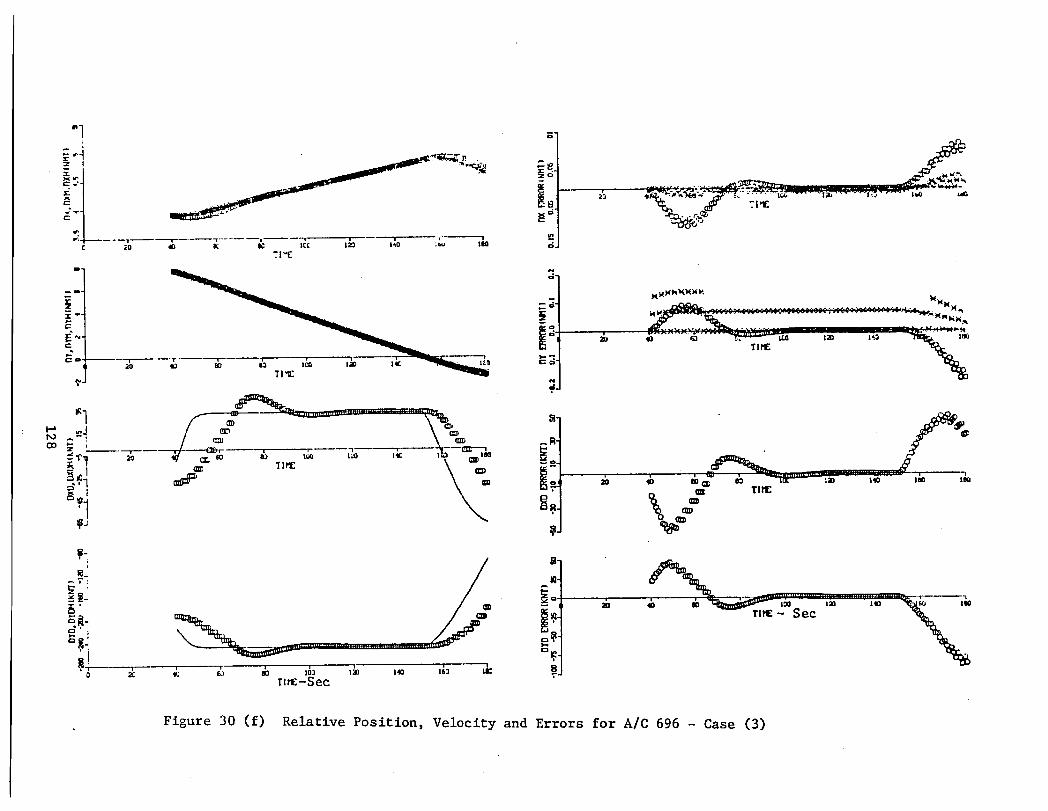
D
-I-_E
TIE
----- _0
TI'IE Oo
,_.
m TIIIf:
_-
,_-
_' _ _+. -'=Se_'= "
o:1 .....................................o+._ '_. .
tx_-Sec
Figure 30 (f) Relative Position, Velocity and Errors for A/C 696 - Case (3)

"[RUENORTH-EA5THRTOWN MERSUREDNORTH-ERST ESTIMATEDNORTH-EA5TIq- I_-
_s2
D
• _1_96
_o. _=_0_._ _-°,_boo o
° oo,_o°%%I'_ .= - ^_w720
_o _ ,,,,,,,z20 4_ °"., _1t_o_%"";°s='2° a_ 4_ °'-., ,_eo_,to, .:-o
Figure 31(a) Horizontal Projection for Case (4)p

Figure 3l(b) Time Line for Case (4)

approximately 12 nmi/inch and the "static display" (the entire track
history dots are seen at once),the measurement noise may have substantially
worse effects on pilots in the CDTI applications. For example, the
display scale may be i nmi/inch and each history dot may be displayed
dynamically as they become available. This means that the linear dimension
would be perceived one order of magnitude larger.
The time line of events for this case - Figure 31(b) - shows one
interesting aircraft (No. 504). It begins as an acquisition aircraft until
= 74 sec; then it transitions to the track region. It then transitions
to the acquisition regions at T = 98.5 sec; and then it transitions back to
the track region at T = 108.5 sec. (Even though not shown, the latter be-
havior is due to Own's altitude maneuver.)
Figures 31(c) through 31(i) show the time plots for all the aircraft
in the track region. All of these show the noise effect. The following
comments summarize the result:
(i) Position measurement errors are between 0.2 ~ 0.4 nmi;
(ii) Position estimation errors are generally smaller due to the
smoothing effect on the _-_ tracker;
(iii) Initial velocity errors are large up to 200 kt; and
(iv) Sampling time variations of i or 2 sec were observed.
This "performance" is thoughtto be realistic. The actual system is
expected to behave worse than the simulation, since many factors are not
incorporated in the simulation program. Two of the important factors are
(a) the correlation process (of establishing between the targets and measure-
ments) is 100% reliable with the simulation programs; and (b) the measurement
errors are assumed to be white noise sequences, whereas for the actual systeml,
the errors would be more correlated due to multi-path and reflection effects.
During the course of debugging and development effort, each module's
inputs and outputs are checked and rechecked to validate the software
comparing with "design" requirements. To that extent the simulation soft-
ware is validated.
131

Figure 3](c) RelativePosition,Velocityand Errors for A/C816 - Case (4)

Figure 31(d) Relative Position, Velocity and Errors for A/C 840 - Case (4)

._ _ o
°_ o° jt'+.,J. gg ° ++;oO
oo
o o'I'c r_ ao too3O
.Oo +:I°o_I_' c .°o°
o o o=_ o o
0
= __ "ty''.'_ _m 4o _ & I_0 _oOD GD
TII_.
Figure 31 (e) RelativePosition,Velocityand Errors for A/C 648 - Case (4)

Figure 31(f) RelativePosition,Velocityand Errors for A/C 768 - Case (4)

Figure 31(g) Relative Position, Velocity and Errors for A/C 696 - Case (4)

Figure 31(h) Relative Position, Velocity and Errors for A/C 504 - Case (4)

Figure 31(i) Relative Position, Velocity and Errors for A/C 552 - Case (4)

CAS Logic Validation
Only certain aspects of the collision avoidance logic were tested,
since it is highly dependent on the chosen encounter scenerios. Valida-
tion efforts are pursued by running selected scenerios, and the simula-
tion results are manually checked to explain discrepancies, if any.
Two methods were used to set up encounterscenerios. Both required
modificationsin the aircraft initializationroutine, ACIC. One was to
simply fix the initialconditionsfor the desiredgeometries. The other
was to choose desiredmiss-distances(in three dimension)at future times
and, by using the randomlyselectedvelocities,the initialpositionsof the
targetswere calculatedback to time O. Therefore,the targetvelocities
were constantbut randomized. There are two significantpoints:
(i) The vertical tracker with the Mode C altitude reports with i00 ft
quantization did not have much effect on the CAS logic output, once
the tracker algorithm was established.
(ii) The randomized (Monte Carlo) selection of tar$et velocities
minimizes any subjective intent in the selected encounter scen-arios. This feature reduces the number of experiements needed
to validate the CAS logic module.
Own aircraftwas allowed to maneuver in pitch in an open-loopman-
ner (not in response to CAS RA advisories). Thus, Own's dynamiceffect
was a factor in the outcome. Figure 32 explainsthe terminologyused in
defining the encounterscenerioin the horizontaldimension. The important
variablesare the range,range rate, Own and targetaltitudesand altitude
rates for defining the encounterin the range and altitudedimension.
Validation of the Proximity and Traffic Advisories were established by
manually checking the computational steps in the DETECT subroutine and
comparing the computer results. This aspect was tested to a certain
139

TARGET
r 'RANGE
RATE RELATIVESPEED
R VRt
INITIALSLANT RANGE
R o
IIII
• IIiI
P1
1MINIMUMSLANT RANGE I
RMIN I
ITCAS UNIT IUNDER TEST
Figure 32. Definitions of Variables Associates
with the Linear Movements of Targets
in the Range Dimension
140

extent by the NASA/Langleypiloted simulationsince PA and TA advisorieswere
used to color code the concernedtrafficwithin the CDTI symBology. It is
noted, however,that the currentand active simulatorversions are different.
The most notable differenceis in the countingprocedures in the threat
detectionlogic. The older versionrelied on the so-calledtwo-out-of-three
rule; whereas the currentversiondoes not have this cushion.
The RAmodules (detection, sense and escape maneuver selections) are
validated in similar ways by mostly manual check of the computation steps.
Table 29 contains a partial list of CAS encounters tested during this effort.
The table lists the initial conditions in terms of Own altitude and altitude
rate, target transponder equippage (2 . ATCRBS and 3 . Node S), relative o
range and range rate, and altitude and altitude rate. These initial conditions
are defined 20 sec before the advisory issuance time. The CAS logic output is
shown in theright most column. For example, Scenario No. I shows that Own
and target are both flying level at Ii,000 and 11,600 feet respectively. The
target is equipped with a Mode C transponder, and the relative range was 6 nmi at
the closing rate of 360 kt (a negative sign indicates that this is a converging
target). Twenty seconds into the encounter, an RA is issued. At that time, the
range and modified range closure times (taus) are 39.5 and 37 sec, respectively.
The specific resolution advisory is a negative (LTENT = i0100 + don't climb).
See Table 26 for the LTENT definitions.
Scenarios (i) through (7) are adopted from the suggested test
scenerios contained in the TCASI II MOPS [2]. These are rather simple
encounters with Own flying level. Scenarios (8) through (i9) are gener-
ated using the Monte Carlo initialization method. Brief discussions are
given below.
Scenario (i): The minimum T (range closure time) is 27 sec which
is smaller than the threshold value of 30 sec at this Own altitude;
the RA threat is declared. The current and future vertical separ-
tion is 600 ft, which is less than the detection threshold of 750
ft, and larger than the RA threshold of 440 ft. Since the threat
is above, the negative "don't climb" advisory is issued.
141

Table 29 CAS Logic ValidationCases
. m . .
z0 z0 Q r r z z Results and Comments
No. (ft) (fps) P (nmi) (kt) (_t) (f_s)
i ii,000 0 2 6.0 -360 11,600 0 TI = 29.5, T2 = 27.0 LTENT = I0100 (DCLM)
2 ii,000 0 2 6.0 1-360 10,760 0 TI = 29.5, x2 = 27.0 LTENT = 00000 (CLM)
3 ii,000 0 2 6.0 -360 11,200 0 TI = 29.5, T2 = 26.3 LTENT = 00100 (DES)
4 Ii,000 0 2 8.0 -500 12,516 -33.3 TI = 33.7, T2 = 29.3 LTENT = I0000 (DDES)
5 ii,000 0 2 8.0 -500 9,517 -33.3 T1 = 33.7, T2 = 28.3 LTENT = 00100 (DES)
6 12,500 0 2 6.0 -360 11,800 0 71 = 29.5, T2 = 22.1 LTENT = 00000 (CLM)
7 12,500 0 2 6.0 -360 12,100 0 71 = 29.5, 72 = 22.2 LTENT = 00100 (DES)
8 21,508 0 3 1.15 -i00 22,513 -13.5 71 = 19.7, T2 = ii.0 LTENT = 00100 (DES)
*Own filter was lagging with _ = -25 ft, _ = 17.7
9 6,033 41.5 2 2 -166 7,190 17.2 TI = 22.1, T2 = 16.8 LTENT = IIII0 (DCLM I000)
I0 24,448 41.5 3 2.1 -I01 27,212 -13.5 .... 71 = 32:5, T2 = 16.9 LTENT = IIIi0 (DCLM i000)
ii 20,903 34.0 2 3.11 -157.2 21,877 22.2 TI = 27.3, _2 = 24.4 LTENT = Iiii0 (DCLM i000)
*Own filter was lagging with _ = 30 ft, z= 13.4

Table 29. CAS Logic Validation Cases Continued
E
Q r £ zI zI ....... Results and CommentsZo ZoNo. (ft) (fps) P (nmi) (kt) (fE) ([ps)
12 8,079 19.4 3 1.27 -105 8,810 -13.5 T1 = 22.8, T2 = 14.2 LTENT = 00000 (CLM)
13 14,079 19.4 3 1.27 -105 14,820 -13.5 TI = 22.8, T2 = 14.2 LTENT = 00000 (CLM)
14 14,337 -35.5 2 2.16 -152 11,437 22.2 TI = 28.6, T2 = 22.9 LTENT = ii001 (DDES 500)
15 26,237-35.5 2 2.16 -152 23,437 22.2 TI = 28.6 T2 = 22.9 LTENT = i0000 (DDES)
16 14,872 -35.5 3 0.03 65.2 14,500 -13.5 TI = 0, T2 = i0 LTENT = I0100 (DCLM)
*Range Divergent
17 26,872 -35.5 3 0.03 68.3 26,500 -13£5 T1 = 0 _2 = 10 LTENT = 10100 (DCIN)
*Range Divergent
18 11,626-41.5 2 1.28-52.1 8,198.... 24:5......il = 32"3'T2 = 26.6LTENT = i0000 (DDES)
19 23,584 -41.5 2 1.26 -52.1 20,222 ....24.5 ........ !l = 31:4' T2 = 25.7 LTENT = 00000 (CLM)

Scenario (2): This situation is similar to (i) except that now the
vertical separation is 340 ft. This is less than the RA threshold.
Because the target is below Own, a positive climb is issued.
Scenario (3): This is similar to (2) except that the threat is 200 ftabove, resulting in a positive "descend" advisory.
Scenario (4): In this scenario, the target is descending at 33.3
fps (2000 rpm). It would be within 540 ft of Own altitude at the
critical time. Since the separation is not within the RA thresholda negative "don't descend" is issued.
Scenario (5): This is a symmetric case of (4). However, the worst
case separation (vertical mlss-dlstance) is within the RA threshold,
and the target will be above during the critical interval; thus, apositive "Descend" is issued.
Scenarios (6) and (7): These cases do not need explanation. See (2)and (3).
Scenario (8): This was a case when Own was in the middle of a
"pitch-down-to-level" maneuver. Consequently the Own altitudeand altltude-rate are in error by -25 ft and 17.7 ft/see, res-
pectively. Figure 33 depicts the situation. Because Own has
leveled-off and the mlss-dlstance would be 460 ft, the correctRA would have been "Don't climb". Because the Own estimator was
lagging the mlss-distance computed from the estimates was in error
by 357 ft resulting in the positive "Descend" advisory. Fortunately,the wrong advisory did not induce a worse situation.
Scenario (9): This case shows an example of a vertical speed limit.
The miss-distance is approximately I00 ft over the critical interval.The target is above throughout the encounter. Thus, the descend
sense is selected. The vertical rate of +2000 fpm is tested, and itfails. But the vertical rate of i000 fpm satisfies the RA threshold.
Therefore, this is selected as the speed limit, resulting in the "Don'tclimb faster than i000 fpm".
144

Alt_tude
22513
t=. 20
22243// Target Altitude_" Profile
22095 s" t=0
21977 "t-_w.I - i
Estimated 21820 t=T2Own 21727 _m
.-_ _" t=_ 2
.- i
//_l 4&---m508 t=Tl t=T2
ActualOwn
Figure 33. Schematic Diagram for Scenario (8)
145

Scenario (I0): The vertical miss-distance is approximately 130
feet. During the critical time period, Own and target altitudes
cross each other. The negative sense is chosen for obvious
reasons. However, if the vertical speed was no faster than i000
fpm, the initial separation will remain safe throughout the critical
time period; thus, a VSL "Don't climb faster than i000 fpm" isselected.
Scenario (ii): This is a wrong advisory case due to Own estimation
errors. Actual RA should be a negative "Don't descend" instead of
"Don't climb faster than i000 fpm".
Scenarios (12) and (13): These two are identical except for altitude.Because the miss-distances were smaller than the threshold value be-
low i0,000 ft; therefore, the RA is identical for both cases.
Scenarios (14) and (15): These two are identical except for thealtitude. The RA vertical threshold is 440 ft for (14), and 640 ft
for (15). The vertical miss-distance is approximately i00 ft below
Own. A positive (climb) sense was chosen. The vertical speed limits
were tested sequentially. The smaller limit was satisfied first for
(14). It took an extra "altitude rate margin" to satisfy the larger
limit for (15). See Figure 34. However, DDES is one "rank" strongerthan DDES 500.
Scenarios (16) and (17): Again, these are identical except for the
altitude. These two cases are continuations of cases (12) and (i0),
respectively, Because of the antenna shadowing due to the pitchmaneuver, this particular target came out on the "other side". Be-
cause of the target proximity, it passed the non-convergent range
test. This is shown as TI being 0 and T2 being limited to i0 sec.
Because the current altitude separation is small for both cases, the
selection logic selects a negative "Do not climb".
Scenarios (18) and (19): These are two identical encounters exceptfor altitude. Because of the difference in threshold values at
different altitudes, the chosen advisories are different. One is
negative (Don't descend), and the other is positive (climb).
146

Altitude
Tcritical
Figure 34. Comparison of VSL's at Different Altitudes
147

Many more encounter scenarios were examined than discussed in the text.
We have reasonable cause to believe that the CAS logic is validated with
respect to the operational and functional characteristics as discussed in the
text. An examination of the test scenario indicates that the major portion
of the CAS logic is captured faithfully in this simulation. The logic was
tested with somewhat benign traffic patterns -no horizontal or vertical
maneuvers by the target. Furthermore, no measurement errors were introduced
to test the CAS logic robustness.
In conclusion, the simulation is validated from the input/output re-
lationship view-point in the following sense:
(a) it obtains operationally correct surveillance/measurement data
given a traffic pattern;
(b) it provides correct position and velocity estimates given thesurveillance data;
(c) it makes correct threat assessment given the estimates; and
(d) it generates correct CAS advisory given the estimates and thethreat assessment.
However, this does not imply that the resultant advisory is "correct"
in avoiding a near-miss because the "correct" position and velocity estimates
do not imply "error-free". It is felt that the altitude measurement and
estimation errors would be the most critical elements.
148

V
CONCLUSIONS
A comprehensive simulation program was developed of the Enhanced
TCAS II system based on the Bendix design. The program is written in
standard Fortran IV, and it is highly transportable among main frame or
mini-computers (CDC-7600, CRAY X-MP, VAX 11/780). The size of the pro-
gram is approximately 3,000 lines of source code including a simple
traffic generation module. It is designed so that it can operate in
seml-real time. There is no reason why the program cannot be installed
into a real-time simulation environment (without any modification), if
the host executive has a one second background priority loop.
Both the traffic sensors and the collision avoidance logic modules are
validated with respect to the known operational characteristics. Some
limitations are imposed, mostly because of convenience and computational
complexity. These are defined in the text.
The program is believed to be a valuable tool, not only for simulation
but also for analysis purposes.
149


APPENDIXA
Major Program Commons
This appendixprovides the list of majorcommonsused by the program. The commons
are listed in Table 18.
151

TABLE A.I/OWNTFL/and/ITLGT/COMMON DEFINITIONS
PROGRAM ENGINEERING
NAME SYMBOL UNIT COMMENTS
TIME t sec System time
XO x0 nmi _ Own north-east coordinate
YO Y0 nml
ZO z0 ft Altitude above MSL
VO v0 kt Ground speed
ATT(1) _ rad
(2) 0 tad __ Attitude angles
(3) _ rad
TBL(I,I) TBL(I,I )
(1,2)
(body to local-level) trans-" " TBL formation
(3,2)
(3,3) TBL(3,3 )
SFO - - NOT ACTIVE
IALO lh0 i00 ft Mode C altitude
RALT hoR ft Radio altitude
AGL
ZGRND _AGL ft Altitude above ground level
ZOM(1) _0 ft Altitude and altitude rate estimates
(2) z0 fps Altitude and altitude rate estimates
(3) Z0m ft Own altitude measurements
NTZO - - Altitude estimate initialization flag
ITRGT - - IDF of pilot selected CDTI target
IWOW - - Weight-on-wheel switch (i . on
ground
MANSEN - - TOAS operating mode (0, I + 2 .
stand-by; 3-7 . manual sensitivity;8 . automatic)
152

TABLE A.2 /BNDXFL/COMMONDEFINITIONS•. _. . ...... ..... • .,..... .
PROGRAM ENGINEERINGNAME SYMBOL UNIT .......... COMMENTS.......
IDF* Target IdentificationNumber
IDM Previous IDF (sign is used as trackerstations
MXN Transpondertype (i .Mode A, 2. Mode C,3 . Mode S)
NXTS = -IIDFI . no need for surveillance
IRPT = 0 . invalidreport
NPOP = 1 . pop-up target
NSTS Advisory statuscounter
TNXT %XT sec Next scheduledsurveillancetime
TLST t.LST sec Last valid surveillancetimeRNGT r nmiBRGT b tad True range,bearingaltitudeALTT zT ftSFT - - NOT ACTIVE
RNGE ~r nml _ Range and bearing errorsBRGE b rad
RNGM rm nmiBRGM b tad " Range and bearingmeasurements
m
EPSM em tad Look-upangle
IALT I_ 100 ft Mode C altitudereportDXM _ nmi %
m _ Measurednorth-eastcomponentsDYM ._Ym nmiDXH Ax nmi \
DYH Ay nmi Horizontal position and velocity estimates
DXDR nmi/secDYDH Ay nmi/sec
DXP Ax+ nmi
DYP AY+ nmi _ Coasted horizontal position
*These are all arrays of twenty.
153

TABLE A.3 /ZTRKCFL/ and /ZWRKVR/Common Definitions
PROGRAM ENGINEERING
NAME SYMBOL UNIT COMMENTS
ICZ* - - Initialization flag; also used as
vertical profile status index
MALT (i)
• lh(ti) i00 ft _ Latest (i = current) five valid Mode
• I C reports corresponding to TMALS.(;)
TMAL(1). 1• ti sec _ Times of latest five valid Mode C
• _ reports(5)
LSV(1) I(2) L(tLS ) i00 ft Latest three Mode C level valuescorresponding to times TSV(3)
TSV(1) 1(2) tLS sec Latest three level,swltchingtimes(s)
TZIC 70 sec Initializationtime
ZSV(1)Altitude inferredat the time of
(2) Zm(tLS) ft devel switchingtimes(3) J
^
ZH zI ft _ Internalattitudeand altituderate
fps _ estimatesZDH zz
ZEXT ZT ftExternal altitude and altitude rate
ZDEXT zT estimates
*These are all arrays of twenty elements
LOSWCH - Level switching flag (i . levelswitched
ITST
TDUMM _ Used as temporary memory; arrays
ZDUMMY _ of five elements.
154

TABLE A.4 /WORKVR/Common Definitions• _ . ...
PROGRAM ENGINEERING .......
NAME SYMBOL UNIT ....... COMMENTS ......
IDENT Temporary identification number
INDEX Temporary file index
ISURV Surveillance flag
IACQ Acqulsitlon/track flag
MDX Transponder type
DXTMP Ax nmi
DYTMP Ay nml Temporary position var iabl es
DZTMP Az ft
ALTMP _h ft
DUNM(1)
(2)
(3)(4)
(5) Temporary working memory
(6)
(7)
(8)
(9)(10)
RANGE Ar nml
BEARG hb tad I Range, bearing and look-up angleEPSI Ae tad
EPSIMX Ae_ tad Maximum look-up and down angle = + 23°
RNGACQ(1) Ar.AcQ nml Maximum search range for Mode A = !7nmi
(2) nmi Maximum search range for Mode C = 17nmi
(3) nmi Maximum search range for Mode S = 25nmi
STMAX VMA X kt Max. target speed (250-600 kt)
RLIM Arrl m nml Min. track range (5 or I0 nmi)
RMIN Ars nmi Track range modification = 1.65 nmi
TAU T hr Track range time period 1/80 hr (= 45 sec
RNGTRK Artr k nmi [ Track region range and altitude boundaryDHI4TRIG nmi _ Computed dynamically
Ahtr k
155

TABLE A.4 /WORKVR/CommonDefinitionsContinued
PROGRAM ENGINEERING...........NAME SYMBOL UNIT ........ COMMENTS.....
TMPWRK(i) _ RNGSQR*
(2) r nmi _ TSTRNG= range computedfrom x and yestimates
(3) _ TSTALT
(4) VDOTP
(5) £ nmi/sec _ RNGDOT = true range rate
(6) _ TSTRRD
(7) Tr sec _ TAUI = range closure time limitedby TVPCMD
(8) _ SPDSQR
(9) T" sec _ TAU2 = modified range closure timer limitedbyITVPCMD
(i0) _ TSTDST
(ii) _' nmi/sec _ RDTMP = range rates limitedbyRDTHR for 0 divide-check
(12) _ DELZD
(13) % DZMOD
ALFAH(8)Horizontaltrackergains. See Table 3.
BETAH(8) 8 I
Q q Mode C altitudequantization= 100 ft.\
- - _THESE SHOULD BE O.SFMX.$IGZ - -
SIGR or nmi Range error standarddeviation= 0.0123nmi
SIGB Ob rad Bearing error standarddeviation= 0.01745Gad
APv ft Surveillancealtitude thresholdDELTH= 250 ft
DELTP APH nmi Surveillancehorizontalpositionthreshold= 0.1645 nmi
IRPTMX - - Number of maximum allowablesurveil-lance failures-i = 4
PRBTHR(1) Surveillancereliabilityfor Mode A =0.9
(2) Prob Surveillancereliabilityfor Mode C =0.95
(3) Surveillancereliabilityfor Mode S =0.99
*Equivalencedin DETECT subroutine. These are mostly temporaryin natureexcept ones with comments. 156

TABLE A.5 /CASFIL/CommonDefinitions• ... • •..... ...... . . ._ . . ... . .. . . _ ..... -............
PROGRAM ENGINEERING ..................NAME SYMBOL..... UNIT COMMENTS.....
eNTADV - Number of threatadvisoriesthis cycle
NCAND+ Identificationof threat candidates
IDCAS Containsthreat IDF of /BNDXFL/
IRACNT 1
ITACNT
ITAFLOT .RA,TA and PA countersand status flags
IPACNT
IPAFLG
TMCNT sec Absolute10 sec timer
IDSTS Advisory statusfla_ (i. PA; 2 . TA:3 . RA and negative. pilot discre-tion)
IDCMD* NOT ACTIVE
TMCAS tCAS sec Time of CAS advisorygeneration
ZDGDAL £DG .fps Individualvertical speed reference
TMCPA tcpA sea Time to CPA
XCPA AXcpA nml )
YCPA AycpA nmi I x, y, z positionat CPADZCPA AZcpA ft
ZDGOUT* _OUT fps Over-allvertical speed referenceNTRA* Number of RA threats
LTENT Packed word
RATEXT* RA test output
*Single variable
+ Array of i0 elements
All others are five element arrays.
157

TABLE A.6 /CWRKVR! and /CWRKV2/Common Definitions
..... . . "....... . " .' -.. ...... .... ... -.-. ........
PROGRAM ENGINEERING
NAME SYMBOL UNIT COMMENTS ......
NDXCAS Number of candidate threats
JDX Temporary CAS file index
NORA No RA capability flag
LVLOW_{ Own sensitivity level
LVLINT Target (and total) sensitivity level
LPA ILTA
I PA, TA, RA Detection flagsLRA
TSTTAU • sec Range closure timer
TAUVRT T sec Altitude closure timev
ZDG £G fps RAvertlcal speed reference
DELZ Az ft Current altitude separation
VMD Az+ ft (Projected) vertical miss-distance
INTENT RApacked word
IHTHR Within threshold (ALMT) flag
LSENSE Climb/descend sense
LDCFLG Don't care flag
LVSLOK Vertical speed limit RA OK flag
LADNOK Advisory Not OK flag
ZMPCLM ft Projected vertical separation for climb
ZMPDES ft Projected vertical separation for des-cend
ZPSECH ft Projected vertical separation forsecond choise
158

TABLE A.7 • /CASPAR/CommonDefinitions
PROGRAM ENGINEERING..................................................NAME SYMBOL UNIT COMMENTS
DMODT ArTA nmi Minimum range guard for TA modifiedtau
DMODR Arp_ nmi Minimum range guard for RAmodifiedtau
TAUTA 8RTA sec TA tau threshold
TAURA 8RRA see RA tau thresholdTVPCMD T sec Vertical tau limit value
vc
HI- 8 [_HRA) nmi2/sec r . _ thresholdfor divergingrange.HTA
RDTHR* _rin nmi/sec Minimum range rate for 0 dividecheck = I0 ktDetectionaltitudeseparationZTHR* 8 ft
Z threshold
DZTHR* _8Z ft Vertical thresholdmodification=.60 ft
ALMT* 8 ft Resolutionaltitude separationa threshold
ZDTHR* fps Minimum vertical speed for 0 dividecheck = -i fps
ZDLVL* NOT ACTIVE
DZDSML* NOT ACTIVE
ZDCMD(7) NOT ACTIVE
KSEQ(6,7) NOT ACTIVE
RCOAL 0RCA nml Minimumrange at co-altitude
RTHRTA eArTA nmt Minimum range threshold
TAILDS nmi Minimum range guard for modifiedtau = 0.247
RTSTMX* nmi Maximum effective RArange = 12 nmi
*S_hgle Variable
All others are five element arrays unless specified.
159


APPENDIX B
DV TCAS II MODEL CONSIDERATIONS
Introduction
In this appendix, DV TCAS II is discussed from the simulation view-
point. The operational characteristics are summarized in Table I. The
DV TCAS II possesses a bearing accuracy of 6-8 deg rms which should be
sufficient for most, if not all, of the perceived CDTI applications.
There are three major differences between the DV TCAS and BX TCAS,
mainly in surveillance functions. These are:
(I) wide angel (90 deg) directive transmit antenna and quadrantmonopulse receiver processing;
(2) regular interrogation interval (I sec); and
(3) aircraft body fixed coordinate system.
The system is essentially a range-altitude system with the angle-
of-arrival (bearing) information used to satisfy the cockpit horizontal
display needs. In order to operate in a high traffic density (0.3 air-
craft/nmi 2) area, extensive use is made of multiple level whisper/shout
interrogations. This is the technique used to minimize "fruit" and
"garbles".
The impacts of items (I) and (2) are several:
(a) smaller effective beam reach;
(b) different internal acquisition/track processing;
(c) somewhat less surveillance reliability which may be rangedependent; and
(d) larger bearing error.
161

The impact of the body fixed corrdinate system results in a distortion
of horizontal projection of the surrounding traffic because the Own body
attitude is unaccounted for.
Implementation of the above aspects into the BX TCAS simulation program
are considered further in the following sections.
Surveillance Function
Coverage volume, reliability and sampler logic. As stated above DV
TCAS does not schedule interrogation. It transmits interrogation pulses
over a 90 deg angular sector every I sec and waits for return signals.
Therefore, the effective coverage is limited by the transmit and the re-
ception power levels. These, in turn, "define" the surveillance reliability
as a function of range. This means that the effective coverage volume is
provided by a suitable surveillance reliability model. Table B.I lists the
probabilities of data drop-out (failed surveillance). It is noted that the
probabilities depends on the range as well as the past drop-out character-
istics. The coverage is given implicitly because the probability distri-
bution depends on the actual range. That is, the probability of obtaining
surveillance data beyond a certain range becomes extremely low; this,
effectively limits the beam reach.
The model is accurate only for the aircraft whose track has been
established. The "aquisition" phase is approximated by giving a small
probability of valid signal reception at an extreme range (say 25 nmi).
Figure B.I Shows a program flow chart which models the sampler logic.
This subroutine must be invoked every second with the actual range and
previous drop-out status. If the surveillance logic is successful, the
routine returns with the flag IRPT set to O; otherwise, the flag is
incremented by i. If the counter becomes 6, then the target is dropped
from the internal track file.
162

Table B.I Probability of DV TCAS Surveillance Data Drop-out
Condition Probability of Data Drop-out
0 < range <I nml 0.i
1 < <2 0.13
2 < <3 0.15
3 < <4 0.15
4 < <5 0.18
5 _ <6 0.21
(6!range < 14).AND.
IRPT (a) = 0 0.27
= 1 0.39
= 2 0.59
ffi3 O.70
= 4 0.79
= 5 0.85
(14 < range < 20).OR.
(b)IRPT ffi 6 0.95
(a) IRPT = Number of consecutive drop-out
(b) Flight test results indicate 1.0
163

START
• +I _ "U'°'_JI
True
<P_GE > 14 .OR. IRPT- 6 >
--+ True ___ > 0+95 _ True ,
alse -
+
_alse ++ ,
Note: Input - RNGE(nmt), IRP'rOutput - IRPTData : PROB/O.1, 0.13, 0.15, 0.15, 0.18, 0.21/
PROB6/0.27, 0.39, 0.59, 0.7, 0.79, 0.85/
Figure B.1 Flow Chart for the DV TCAS Sampler Loy,i c.
164

It is noted that the drop-out model was obtained for the so-called
omn.i-directional active BCAS (which is a direct predecessor of DV TCAS II)
based on flight test results. The reliability performance may have improved
substantially since BCAS because of two design improvements: 90 deg
antenna directivity and multi-level whisper/shout power sequencing.
Estimation
There are two requirements for the estimation functions within DV TCAS.
One is the need for internal traffic file management including the target
and measurement correlation by means of a gating technique. The other is
the CAS logic requirement. As mentioned above, these are performed along
the range and altitude axes. Therefore, the entire estimation functions
are developed along these axes.
An alternative is to use the current algorithm and approximate the
inverse transformation, as given in Eq (19). That is, the measured Ax and
Ay are given by
hx = hr cos (_ + hb) ,
(B.I)AY = Ar sin (_ + Ab) •
here,
Ar = range ,
Ab = bearing ,
and
= Own heading.
The resulting Ax and Ay measurements are then input to the filter algorithm
module.
It is noted that the approximation given by Eq. (B.I) is fairly
accurate if the roll and pitch angles are small. Also, it can be used to
support a horizontal CRT display unit in the cockpit.
165

With the above two adjustments, the remainder of the simulation program
should stay intact. By increasing the bearing noise level to 6-8 deg, the
resultant program can be used to support the CDTI research effort reflecting
a less capable system than BX TCAS.
166

REFEFENCES
i_ Goka, T., "Analysis of Estimation Algorithms for CDTI and CAS
Applications, " NASA CR-172444, 1984.
12. Anon., "Minimum Operational Performance Standards for Traffic
Alert and Collision Avoidance System (TCAS) - Final Draft",
RTCA Paper No. I06-83/SC KT-RO, Radio Technical Commission forAeronautics, Washington, D.C., March 1983.
3. Sobocinski, R., "Flight Test Results with Collision Avoidance
Systems," Paper No. 20-2. Proceed. of the Digital AvionicsSystems Conf., Seattle, WA, October 1983.
4. Reed, J.E., "Enhanced TCAS II Test Results", Paper No. 20-3,
Proceed. of 5th Digital Avionics Systems Conf., Seattle, WA,October 1983.
5. Anon., "Full BCAS Critical Design Review for the EngineerngModel--Task i", Bendix Corp., Communications Division, Baltimore,
MD, September 1981.
6. Read, J.E., "TCAS-II Engineering Model Design specification(Model A and Model B)--Revision II, "Report No. BCD-TR-0063,
Bendix Corp., Baltimore, MD, April 1982.
7. Sinsky, A.I., and B. J. Tier, "Coordinate Transformation Algorithms",
Report No. BCD-TN-82-020, Bendix Corp., Baltimore, MD, May 1982.
8. Sinsky, A. I., "Alpha-Beta Tracking Errors for Orbiting Targets,"
Report No. BCD-TN-81-033, Bendix Corp., Baltimore, MD, June 1981.
9. Andrews, J. W., "An Improved Technique for Altitude Tracking of
Aircraft," FAA Report No. ATC-105, MIT/Lincoln Laboratory,
Lexington, MA, 1980.
I0. Billman, B. R., "Analysis of a Nonlinear Altitude Tracking Method,"
FAA Report No. FAA RD-81-60A, FAA Technical Center, Atlantic
City, NJ, February 1982.
167
I


_ 1. Report No. 2. Government Acc_ion No. 3. R_ipient's _l_ No.
NASA CR-172445
4. Title and Subtitle 5. Re_ Date
ENHANCED TCASII/CDTI TRAFFIC SENSOR OCTOBER 1984DIGITAL SIMULATION MODEL AND 6. Pe_ormingOr_nization_de
PROGRAM DESCRIPTION
7. Aut_r(s) 8. Performing Or_nization Report No.
Tsuyoshi Goka10. W_k Unit No.
9. Puf_ming Or_nization Name and Address
Analytical Mechanics Associates, Inc. '11. _ntract or Grant No.2483 Old Middlefield Way
Mountain View, California 94043 NASI-1613513. Ty_ of Repo_ and P_iod _ver_
12. S_nsoring A_y Name _d Address Contractor Report
National Aeronautics and Space Administration 14. SponsoringAgency_Washington, DC 20546
15. _p_ementary Not_
Langley Technical Monitors: Roland L. Bowles and David H. Williams
Final Report
16. Abstract
The objectives of this project were to develop digital simulation models ofenhanced TCAS II/CDTI traffic sensors based on actual or projected operational
and performance characteristics. Two enhanced Traffic (or Threat) Alert andCollision Avoidance Systems were considered. The main focus is a system based
on the FAA/Bendix design which dates back to the so-called full Beacon
Collision Avoidance System (BCAS) concept. The other system is built by Dalmo
Victor Division of Textron's Bell Aerospace Co. based on the FAA/MIT active
BCAS concept.
Based on the engineering model, a digital simulation program was developed in
FORTRAN. The program contains an executive with a semi-real time batch
processing capability. Thus, the simulation program can be interfaced with
other modules with a minimum requirement. The program is described in detail.
Both the traffic sensor and CAS logic modules are validated by means ofextensive simulation runs. Selected validation cases are discussed in detail,
and capabilities and limitations of the actual and simulated systems are noted.
The TCAS systems are not specifically intended for Cockpit Display of Traffic
Information (CDTl)applications. However, these systems are sufficiently
general to allow implementation of CDTI functions within the real systems'constraints.
17. Key Wor_ (Suggest_ by Author(s)) 18. Distribution Statement
CDTI
Traffic Sensor Unclassified - UnlimitedTCAS SIMULATION
19. Security Classif.(of this report} 20. Security Classif. (of this page) 21, No. of Page_ 22. Price
Unclassified Unclassif led 167
.-30s ForsalebytheNationalTechnicalInformationService,Springfield,Virginia2216!


r
.-r
. f
f
.
o
_ o ..1
i .!
L