enhancement of uncoupled nonlinear equations method for determining kinetic parameters in case of...

i n t e r n a t i o n a l j o u r n a l o f h y d r o g e n e n e r g y 3 4 ( 2 0 0 9 ) 1 6 5 5 – 1 6 6 3

Avai lab le a t www.sc iencedi rec t .com

j ourna l homepage : www.e lsev ier . com/ loca te /he

Enhancement of uncoupled nonlinear equations method fordetermining kinetic parameters in case of hydrogen evolutionreaction after dropping two assumptions

Mukesh Bhardwaj

Department of Metallurgical and Materials Engineering, National Institute of Technology, Durgapur 713209, West Bengal, India

a r t i c l e i n f o

Article history:

Received 21 August 2008

Received in revised form

9 December 2008

Accepted 10 December 2008

Available online 11 January 2009

Keywords:

Hydrogen evolution reaction

Volmer–Heyrovsky–Tafel

mechanism

Volmer–Heyrovsky

mechanism

Electrochemical impedance

spectroscopy

Tafel polarization

Heyrovsky backward reaction rate

Tafel backward reaction rate

Symmetry factors

E-mail address: mukesh_bhardwaj_india0360-3199/$ – see front matter ª 2008 Interndoi:10.1016/j.ijhydene.2008.12.017

a b s t r a c t

Hydrogen evolution reaction involves three reaction steps, i.e., Volmer, Heyrovsky and

Tafel. Out of six kinetic parameters, only four are independent. Tafel polarization and

alternating current admittance data at various frequencies and at various overpotentials

can be utilized for obtaining values of independent kinetic parameters. In the previous

work [Bhardwaj M, Balasubramaniam R. Uncoupled nonlinear equations method for

determining kinetic parameters in case of hydrogen evolution reaction following Volmer–

Heyrovsky–Tafel mechanism and Volmer–Heyrovsky mechanism. Int J Hydrogen Energy

2008;33:2178–88], uncoupled nonlinear equations methods for determining kinetic

parameters in case of systems following Volmer–Heyrovsky–Tafel mechanism and

Volmer–Heyrovsky mechanism were developed. In that work, Heyrovsky and Tafel back-

ward reaction rates were neglected and Volmer and Heyrovsky symmetry factors were

assumed equal to half for obtaining the values of kinetic parameters. In the present work,

both of these assumptions have been dropped and uncoupled nonlinear equations have

been re-derived. The equations have been validated using literature data.

ª 2008 International Association for Hydrogen Energy. Published by Elsevier Ltd. All rights

reserved.

1. Introduction steps, i.e., Volmer, Heyrovsky and Tafel [1]. These are shown

Hydrogen evolution reaction (HER) is an important reaction in

aqueous electrochemistry. Some of the main factors govern-

ing the kinetics of HER are electrolyte composition, pH,

temperature, pressure, electrode physical and chemical

nature and the applied potential. In order to characterize the

kinetics of HER, the experimental parameters are transformed

into kinetic parameters via a kinetic model (or constitutive

equations). The kinetic model for HER follows three reaction

@yahoo.comational Association for H

below.

Volmer ðvÞ MþHþ þ e�#MHads (1)

Heyrovsky ðhÞ MHads þHþ þ e�#MþH2 (2)

Tafel ðtÞ MHads þMHads#2MþH2 (3)

Assuming Langmuir adsorption isotherm, the constitutive

equations [1] for the kinetic model can be written as

ydrogen Energy. Published by Elsevier Ltd. All rights reserved.

mailto:[email protected]

http://www.elsevier.com/locate/he


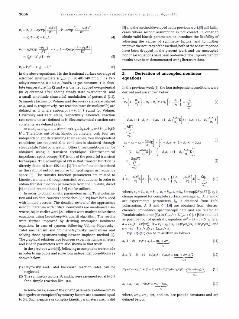
vv ¼ kvð1� qÞexp

��bvFh

RT

�� k�vqexp

�ð1� bvÞFh

RT

�
¼ k0vð1� qÞ � k0�vq (4)
vh ¼ khqexp

��bhFh

RT

�� k�hð1� qÞexp

�ð1� bhÞFh

RT

�¼ k0hq� k0�hð1� qÞ (5)

vt ¼ ktq2 � k�tð1� qÞ2 (6)

In the above equations, q is the fractional surface coverage of

adsorbed intermediate (Hads), F¼ 96,485.340 C mol�1 is Far-

aday’s constant, R¼ 8.314 J/mol/K is gas constant, T is abso-

lute temperature (in K) and h is the net applied overpotential

(in V) obtained after adding steady state overpotential and

a small amplitude sinusoidal modulation of potential [1,2].

Symmetry factors for Volmer and Heyrovsky steps are defined

as bv and bh respectively. Net reaction rates (in mol/cm2/s) are

defined as vi where subscript i¼ v, h, t stand for Volmer,

Heyrovsky and Tafel steps, respectively. Chemical reaction

rate constants are defined as ki. Electrochemical reaction rate

constants are defined as ki0.

At h¼ 0, vv¼ vh¼ vt¼ 0 implies k�h¼ khkv/k�v and k�t¼ ktkv2/

k�v2 . Therefore, out of six kinetic parameters, only four are

independent. For determining their values, four independent

conditions are required. One condition is obtained through

steady state Tafel polarization. Other three conditions can be

obtained using a transient technique. Electrochemical

impedance spectroscopy (EIS) is one of the powerful transient

techniques. The advantage of EIS is that transfer function is

directly obtained from EIS data [3]. Transfer function is defined

as the ratio of output response to input signal in frequency

space [3]. The transfer function parameters are related to

kinetic parameters through constitutive equations. In order to

obtain transfer function parameters from the EIS data, direct

[4] and indirect methods [1,5,6] can be utilized.

In order to obtain kinetic parameters using Tafel polariza-

tion and EIS data, various approaches [2,7–19] have been used

with limited success. The detailed review of the approaches

used in literature with critical comments are mentioned else-

where [20]. In earlier work [21], efforts were made to solve these

equations using Levenberg–Marquardt algorithm. The results

were further improved by deriving uncoupled nonlinear

equations in case of systems following Volmer–Heyrovsky–

Tafel mechanism and Volmer–Heyrovsky mechanism and

solving those equations using Newton–Raphson method [5].

The graphical relationships between experimental parameters

and kinetic parameters were also shown in that work.

In the previous work [5], following assumptions were made

in order to uncouple and solve four independent conditions as

shown below.

(1) Heyrovsky and Tafel backward reaction rates can be

neglected.

(2) The symmetry factors, bv and bh were assumed equal to 0.5

for a simple reaction like HER.

In some cases, some of the kinetic parameters obtained may

be negative or complex if symmetry factors are assumed equal

to 0.5. Such negative or complex kinetic parameters are invalid

[5] and the method developed in the previous work [5] will fail in

cases where second assumption is not correct. In order to

obtain valid kinetic parameters, to introduce the flexibility of

adjusting the values of symmetry factors, and to further

improve the accuracy of the method, both of these assumptions

have been dropped in the present work and the uncoupled

nonlinear equations have been re-derived. The improvement in

results have been demonstrated using literature data.

2. Derivation of uncoupled nonlinearequations

In the previous work [5], the four independent conditions were

derived and are shown below.�x3

�1þ x1

x2E

�� x1 � x2

�qþ x1

�1� x3

x2E

�¼ �iss

F|{z}m1

(7)

��bvx1þð1�bvÞx2þbhx3�ð1�bhÞ

x3x1

x2E

�qþ�

bvx1þð1�bhÞx3x1

x2E

�

¼ARTF2|ffl{zffl}

m2=2

(8)�x1 þ x2 � x3 �

x3x1

x2E

�� bvx1 þ ð1� bvÞx2 � bhx3� � ��

þ ð1� bhÞx3x1

x2E q� � bvx1 þ ð1� bhÞ

x3x1

x2E

¼ �Bq1RTF3|fflfflfflfflffl{zfflfflfflfflffl}

m3=2

(9)

4

�x4 �

x4x21

x22

E

�qþ

�x1 þ x2 þ x3 þ

�x3x1

x2þ 4

x4x21

x22

�E

�¼ Cq1

F|{z}m4

(10)

where, x1¼ k0

v, x2¼ k0

�v, x3¼ k0

h, x4¼ kt, E¼ exp(2Fh/(RT )). q1 is

charge required for complete surface coverage. iss, A, B and C

are experimental parameters. iss is obtained from Tafel

polarization. A, B and C [1,6] are obtained from electro-

chemical impedance spectroscopy data and are related to

Faradaic admittance (Yf) as Yf¼Aþ B/( juþ C ). q [5] is obtained

as positive root of quadratic equation aq2þ bqþ c¼ 0, where,

a¼ 2x4(1� Ex12/x2

2), b¼ x1þ x2þ x3þ E(x1/x2)(x3þ 4x4x1/x2) and

c¼�x1� E(x1/x2)(x3þ 2x4x1/x2).

Eqs. (7)–(10) can be re-written as follows.

x1ð1� qÞ � x2qþ x3q ¼ m1 þ dm1|fflfflfflfflfflffl{zfflfflfflfflfflffl}r1

(11)

bvx1ð1� qÞ þ ð1� bvÞx2qþ bhx3q ¼ ðm2 þ dm2Þ=2|fflfflfflfflfflfflfflfflfflfflffl{zfflfflfflfflfflfflfflfflfflfflffl}r2=2

(12)

½x1þx2�x3�½bvx1ð1�qÞþð1�bvÞx2q�bhx3q�¼ðm3þdm3Þ=2|fflfflfflfflfflfflfflfflfflffl{zfflfflfflfflfflfflfflfflfflffl}r3=2

(13)

x1 þ x2 þ x3 þ 4x4q ¼ m4 þ dm4|fflfflfflfflfflffl{zfflfflfflfflfflffl}r4

(14)

where, dm1, dm2, dm3 and dm4 are pseudo-constants and are

defined below.

i n t e r n a t i o n a l j o u r n a l o f h y d r o g e n e n e r g y 3 4 ( 2 0 0 9 ) 1 6 5 5 – 1 6 6 3 1657

dm1 ¼x3x1

x2ð1� qÞE (15)

dm2 ¼ �2ð1� bhÞdm1 (16)

dm3 ¼2x3x1

xE

�bvx1ð1� qÞ þ ð1� bvÞx2q� bhx3q

2

þ ð1� bhÞðx1 þ x2 � x3Þð1� qÞ � x3x1

x2Eð1� bhÞð1� qÞ

�ð17Þ

dm4 ¼ �E

�x3x1

x2þ 4

x4x21

x22

ð1� qÞ�

(18)

In order to solve Eqs. (11)–(14), it is necessary to first obtain the

values of these pseudo-constants. Therefore, iterative method

is used for solving these equations. In first iteration, the values

of these pseudo-constants is taken as zero. The roots of the

equations are thus obtained in the first iteration neglecting

Heyrovsky and Tafel backward reaction rates similar to the

method discussed elsewhere [5]. For subsequent iterations,

the values of pseudo-constants are obtained using values of

x1, x2, x3 and x4 obtained in the preceding iteration. The

equations are again solved to obtain the roots. This iterative

process is continued till the magnitude of change in value of

any of the root between two consecutive iterations exceeds

a specified small value. This analysis is valid for E� 1, i.e., for

sufficiently large cathodic overpotentials. It may be noted that

E¼ 0.21 at h¼�20 mV and T¼ 298 K.

In further discussion, Eqs. (11)–(14) will be uncoupled for

systems following Volmer–Heyrovsky–Tafel mechanism and

Volmer–Heyrovsky mechanism using similar approach as

discussed elsewhere [5].

2.1. Volmer–Heyrovsky–Tafel mechanism

The equation for q can be re-written as shown below.

q ¼x1 þ E

�x3x1

x2þ 2

x4x21

x22

�

x1 þ x2 þ x3 þ 2x4qþ E

�x3x1

x2þ 2ð2� qÞx4x2

1

x22

� (19)

In a fraction, subtraction of small terms in both numerator

and denominator does not significantly affect its value.

Therefore, for E� 1, equation for q can be simplified to Eq.

(20). Using Eq. (14), Eq. (20) can be derived.

q ¼ x1

x1 þ x2 þ x3 þ 2x4q¼ x1= ðr4 � 2x4qÞ|fflfflfflfflfflfflfflffl{zfflfflfflfflfflfflfflffl}

p4

(20)

This results in the following equations.

q ¼ r4 �ffiffiffiffiffiffiffiffiffiffiffiffiffiffiffiffiffiffiffiffiffiffir2

4 � 8x1x4

p4x4

(21)

p4 ¼r4 þ

ffiffiffiffiffiffiffiffiffiffiffiffiffiffiffiffiffiffiffiffiffiffir2

4 � 8x1x4

p2

(22)

Multiplying both sides of Eq. (11) by (1� bv), adding Eq. (12) and

re-arranging terms, following equation can be obtained.

x3q ¼ x3x1

p4¼ 1

1� bv þ bh

h�1� bv

r1 þ

r2

2� x1ð1� qÞ

i(23)

Multiplying both sides of Eq. (11) by bv, subtracting it from Eq.

(12) and re-arranging terms, following equation can be

obtained.

x2q ¼ x2x1

p4¼ r2

2� bvr1 þ ðbv � bhÞx3q (24)

Eq. (11) can be solved to obtain the following equation.x1 þ x2 � x3 ¼

x1 � r1

q(25)

Using Eq. (12), expression [bvx1(1� q)þ (1� bv)x2q� bhx3q] is

equal to the expression (r2/2� 2bhx3q) and can be solved as

follows.

r2

2� 2bhx3q ¼ 1

1� bv þ bh

h2bhx1ð1� qÞ þ ð1� bv � bhÞ

r2

2

� 2ð1� bvÞbhr1

i(26)

Substituting Eqs. (25) and (26) in Eq. (13) and on solving

following equation is obtained.

p4 ¼x1

q¼ x1

�1

x1 � r1

�|fflfflfflfflfflffl{zfflfflfflfflfflffl}

x11

266664

4bhx1ðx1 � r1Þ þ r3ð1� bv þ bhÞ|fflfflfflfflfflfflfflfflfflfflfflfflfflfflfflfflfflfflfflfflfflfflfflfflfflfflfflfflfflffl{zfflfflfflfflfflfflfflfflfflfflfflfflfflfflfflfflfflfflfflfflfflfflfflfflfflfflfflfflfflffl}x121

4bhx1 þ ð1� bv � bhÞr2 � 4ð1� bvÞbhr1|fflfflfflfflfflfflfflfflfflfflfflfflfflfflfflfflfflfflfflfflfflfflfflfflfflfflfflfflfflfflfflfflfflfflfflfflfflffl{zfflfflfflfflfflfflfflfflfflfflfflfflfflfflfflfflfflfflfflfflfflfflfflfflfflfflfflfflfflfflfflfflfflfflfflfflfflffl}x122

377775(27)

Substituting expression for p4, following equation is obtained.

X1 ¼ x11x121=x122

x4 ¼r2

4 � ð2x1X1 � r4Þ2

8x1¼ X1ðr4 � x1X1Þ

2

(28)

Substituting expressions for x2, x3, x4 and q in Eq. (14), equation

in one variable (x1) is obtained as discussed elsewhere [5].

Following first order differentials are required for obtaining

solution using Newton–Raphson method.

dx2

dx1¼ �

hr2

2� bvr1

i 1

q2

dq

dx1þ ðbv � bhÞ

dx3

dx1(29)

dx3

dx1¼ 1

1� bv þ bh

��nð1� bvÞr1 þ

r2

2

o 1

q2

dq

dx1� dp4

dx1þ 1

�(30)

dx4

dx1¼ 1

2

�ðr4 � 2x1X1Þ

dX1

dx1� X2

1

�(31)

dX1

dx1¼ 1

x122

�x121

dx11

dx1þ x11

dx121

dx1� X1

dx122

dx1

�(32)

dx11

dx1¼ � 1

ðx1 � r1Þ2(33)

dx121

dx1¼ 4bhð2x1 � r1Þ (34)

dx122

dx1¼ 4bh (35)

dq

dx1¼ 1

p4

�1� x1

p4

dp4

dx1

�(36)

dp4

dx1¼ �2

x4 þ x1dx4dx1

2p4 � r4(37)

Table 1 – Electrode and electrolyte used in literature forHER.

Exp. Reference Electrode Electrolyte

Volmer–Heyrovsky–Tafel mechanism

1 Bai et al. [2] Activated Pt 0.5 M NaOH at 296 K

2 Fournier et al. [22] Ru/C/LaPO4 1 M KOH at 298 K

3 Okido et al. [10] Ni–Al–Cr–Cu 5.36 M KOH at 343 K

4 Barber and Conway [14] Pt (111) plane 0.5 M NaOH at 296 K

Volmer–Heyrovsky mechanism

5 Chen and Lasia [23] 70Ni–30Zn 1 M NaOH at 298 K

6 Lasia and Rami [24] Ni 1 M NaOH at 298 K


2.2. Volmer–Heyrovsky mechanism

In case of system following Volmer–Heyrovsky mechanism,

Tafel step is not available. Therefore, q is given by the

following equation.

q ¼ x1

x1 þ x2 þ x3(38)

Substituting q in Eq. (11), following equation is obtained.

1x1

�1þ x2

x3

�þ 1

x3¼ 2

r1(39)

Multiplying Eq. (11) by bv, subtracting resulting equation from

Eq. (12), substituting q and on solving, following equation is

obtained.

1x1

�1þ x3

x2

�þ 1

x2¼ 2

r2 � r1ðbv þ bhÞ(40)

In order to obtain the values of three independent kinetic

parameters (kv, k�v and kh), three independent conditions are

necessary. The available conditions are Eqs. (11) and (12). One

additional condition is obtained knowing the fact that at

a very large cathodic overpotentials, Volmer backward reac-

tion rate can be neglected. Thus, at lower h (more cathodic

overpotential), x2/0. Therefore, Eqs. (39) and (40) reduces to

Eqs. (41) and (42) respectively.

1x1þ 1

x3¼ 2

r1(41)

r2 ¼ r1ðbv þ bhÞ (42)

Thus, the value of (bvþ bh) can be obtained as r2/r1 at a more

cathodic overpotential.

For convenience, we represent expression exp[�bvFh/(RT )]

by ev, exp[(1� bv)Fh/(RT)] by e�v and exp[�bhFh/(RT)] by eh. At

lower h, we represent ev by evl, eh by ehl and r1 by r1l.

Eq. (41) at a lower h can thus be expressed as Eq. (43).

1kv¼ 2evl

r1l� evl

ehl

1kh

(43)

Substituting Eq. (43) in Eq. (39), following equations are

obtained.�2evl

r1l� evl

ehl

1kh

��1þ e�v

eh

k�v

kh

�þ ev

eh

1kh� 2ev

r1¼ 0 (44)

1

2k2h

��ehl

r1l� 1

2e�vk�v

�eh�ev

ehl

evl

��|fflfflfflfflfflfflfflfflfflfflfflfflfflfflfflfflfflfflfflfflfflfflfflfflffl{zfflfflfflfflfflfflfflfflfflfflfflfflfflfflfflfflfflfflfflfflfflfflfflfflffl}

b1

1khþ ehleh

evle�vk�v

�ev

r1�evl

r1l

�¼0 (45)

1kh¼ b1 �

ffiffiffiffiffiffiffiffiffiffiffiffiffiffiffiffiffiffiffiffiffiffiffiffiffiffiffiffiffiffiffiffiffiffiffiffiffiffiffiffiffiffiffiffiffiffiffiffiffiffib2

1 �2ehleh

evle�vk�v

�ev

r1� evl

r1l

�s|fflfflfflfflfflfflfflfflfflfflfflfflfflfflfflfflfflfflfflfflfflfflfflffl{zfflfflfflfflfflfflfflfflfflfflfflfflfflfflfflfflfflfflfflfflfflfflfflffl}

M

(46)

Substituting Eq. (43) in Eq. (40), following equations are

obtained.

�2evl

r1l� evl

ehl

1kh

��1þ eh

e�v

kh

k�v

�þ ev

e�v

1k�v� 2ev

r2 � r1ðbv þ bhÞ¼ 0 (47)

1

2k2��ehl

r� evehl

e fr �r ðb þb Þg�1

2e k

�eh�ev

ehl

e

��1k� ehleh

r e k¼0

h 1l vl 2 1 v h �v �v vl|fflfflfflfflfflfflfflfflfflfflfflfflfflfflfflfflfflfflfflfflfflfflfflfflfflfflfflfflfflfflfflfflfflfflfflfflfflfflfflfflfflfflfflfflfflffl{zfflfflfflfflfflfflfflfflfflfflfflfflfflfflfflfflfflfflfflfflfflfflfflfflfflfflfflfflfflfflfflfflfflfflfflfflfflfflfflfflfflfflfflfflfflffl}b2

h 1l �v �v

(48)

1kh¼ b2 þ

ffiffiffiffiffiffiffiffiffiffiffiffiffiffiffiffiffiffiffiffiffiffiffiffiffiffiffiffiffiffib2

2 þ2ehleh

r1le�vk�v

s|fflfflfflfflfflfflfflfflfflfflfflfflffl{zfflfflfflfflfflfflfflfflfflfflfflfflffl}

N

(49)

In Eq. (49), only positive root is considered as N is always

greater than the terms outside square root. Comparing, Eqs.

(46) and (49), the following error function, f is obtained.

f ¼ NHM� evehl

evlfr2 � r1ðbv þ bhÞg(50)

Eq. (50) can be solved to obtain value of k�v. In order to obtain

solution of k�v, only negative sign can be considered between

N and M in Eq. (50). The following first order differentials are

required for obtaining solution using Newton–Raphson

method.

dMdð1=k�vÞ

¼ � 12Me�v

�b1

�eh � ev

ehl

evl

�þ 2ehleh

evl

�ev

r1� evl

r1l

��(51)

dNdð1=k�vÞ

¼ � 12Ne�v

�b2

�eh � ev

ehl

evl

�� 2ehleh

r1l

�(52)

3. Results and discussion

The approach to solve uncoupled equations using Newton–

Raphson method is similar to the approach mentioned else-

where [5,20]. In previous method [5], there was only one

empirical parameter (q1) in case of a system following Volmer–

Heyrovsky–Tafel mechanism. In present method, there are

three empirical parameters (q1, bv and bh). The value of q1 is

not required in case of system following Volmer–Heyrovsky

mechanism and the empirical parameters are only two (bv and

bh). The values of empirical parameters are tuned to obtain

a set of all the positive kinetic parameters with best fittings

between all the experimental parameters and the kinetic

parameters.

In order to validate the present method, the results will be

compared with the experimental data given in literature

[2,5,10,22,23]. The method used in the literature will also be

Table 2 – The experimental parameters utilized for calculation of kinetic parameters as shown in Table 3.

Exp. Reference h, mV iss, mA cm�2 A, U�1 cm�2 B, U�1 cm�2 s�1 C, s�1


1 Bai et al. [2] �142 �2.815 0.083 �30.2 725

2 Fournier et al. [22] �75 �36.04 1.525 �2.235 5.144

3 Okido et al. [10] �56 �54.95 1.681 �0.296 2.015

4 Barber and Conway [14] �75 �1.150 0.069 �18.245 300


5 Chen and Lasia [23] �50.6 �0.018 9.68� 10�4

�231 �3.585

6 Lasia and Rami [24] �20.6 �0.001 5.30� 10�5

�341 �0.751


briefly explained. The electrode and electrolyte used in liter-

ature are shown in Table 1. The experimental parameters

utilized for calculation of kinetic parameters are shown in

Table 2. The valid kinetic parameters fitting experimental data

are shown in Table 3. The invalid kinetic parameters (being

either negative or complex number) are also shown in the

table and are marked with asterisk (*). The calculated values of

iss, A, B, C and q versus overpotential (h), using kinetic

parameters obtained in present method and that given in

literature are compared with the experimental data (Figs. 1–6).

In the figures, the scattered dots show experimental data, the

solid lines show fittings using valid kinetic parameters

obtained in present method and dotted lines show fittings

using kinetic parameters given in literature. The vertical

arrows in the figures show the overpotentials utilized for

calculating kinetic parameters using the present method.

In case of systems following Volmer–Heyrovsky–Tafel

mechanism, four examples have been taken from literature in

chronological order. In 1987, Bai et al. [2] manipulated various

Table 3 – The kinetic parameters calculated using experimentahave not been shown in cases where they were assumed equa

Exp. Reference kv, mol/cm2/s� 1010

k�v, mol/cm2/s� 1010


1 Bai et al. [2] 100 3000

Bhardwaj (this study) 84 2277

2 Fournier et al. [22] 520� 180 74� 18

Bhardwaj (this study) 4558 11,214


3 Okido et al. [10] 2980 895,000



4 Barber and Conway [14] 130� 20 7000� 1000

Bhardwaj et al. [5] 553 591



5 Chen and Lasia [23] 0.63� 0.04 1200� 3000

Bhardwaj (this study) Complex* Complex*

Bhardwaj (this study) 0.681 159

6 Lasia and Rami [24] 0.042� 0.01 (4� 0.1)� 109� kh

Bhardwaj and

Balasubramaniam [5]

0.190 0.265

Bhardwaj (this study) 0.304 0.130

The asterisk mark (*) indicates invalid data due to either negative or com

values of kinetic parameters in the computer, until for one set of

values, sufficiently good agreement was obtained between the

numerically evaluated and experimental values for HER at

activated Pt in 0.5 M NaOH at 296 K. The results have been

compared in Fig. 1. The fittings obtained using both the methods

are good. In present method, all the curves pass through the

experimental data at an overpotential utilized for calculating

kinetic parameters and is generally true in all cases. Using

present method, bv¼ 0.47 and bh¼ 0.42 resulted in best fittings.

Thus, comparing present method with the previous method [5],

dropping both the assumptions resulted in improved fittings. It

may be noted that the drop of first assumption always lead to

more accurate kinetic parameters, thus improving fittings

particularly for data at a very less cathodic overpotentials.

In 1992, Fournier et al. [22] minimized the average of

standard deviations between experimental and calculated

values for (i) iss, A, B, C and (ii) iss, A, B/C as a function of h for

HER at Ru/C/LaPO4 electrode in 1 M KOH at 298 K. The method

utilized to choose kinetic parameters for minimizing average

l parameters as shown in Table 2. The values of bv and bh

l to 0.5.

kh, mol/cm2/s� 1010

kt, mol/cm2/s� 1010

q1, mC/cm2 bv bh

2 280 70

8 163 24.3 0.47 0.42

2000� 300 31,000� 4000 0.57� 0.08

758 �1239* 40,000 0.50 0.50

312 46 40,000 0.60 0.69

27,200 18� 106 64� 105

2034 �2115* 109,000 0.50 0.50

989 677 109,000 0.70 0.73

0.86� 0.1 150� 20 60� 20

1.28 67 90

0.76 70 90 0.49 0.50

96� 220 0.66

Complex* 0.50 0.50

26.53 0.68 0.32

>10

0.0689

0.0607 0.50 0.50

plex (i.e., nonreal) kinetic parameter.

Fig. 1 – Plot of iss, A, B, C and q for HER at activated Pt in

0.5 M NaOH at 296 K. The scattered dots represent

experimental data of Bai et al. [2]. The dotted lines show

calculated data using kinetic parameters of Bai et al. [2].

The solid lines show calculated data using kinetic

parameters obtained in present approach. The vertical

arrows indicate the overpotential utilized for calculating

kinetic parameters.

Fig. 2 – Plot of iss, A, B, C and q for HER at Ru/C/LaPO4

electrode in 1 M KOH at 298 K. The scattered data show

experimental data of Fournier et al. [22]. The dotted lines

show calculated data using kinetic parameters of Fournier

et al. [22]. Other symbols have the same meaning as

mentioned in Fig. 1.


standard deviation was not specified. The results have been

compared in Fig. 2. Improvement in fittings using present

method is evident from the figure. Using present method,

bv¼ 0.60 and bh¼ 0.69 resulted in best fittings. Choosing

bv¼ 0.50 and bh¼ 0.50 for determining kinetic parameters

resulted in negative value of kt as shown in Table 3. In general,

any other or multiple kinetic parameters obtained may be

negative. Thus, previous method [5] fails in determining valid

kinetic parameters. Only present method after dropping

second assumption can result in valid kinetic parameters in

such cases.

In 1993, Okido et al. [10] utilized the 25 factorial method to

choose the values of five kinetic parameters. They minimized

average of variance between experimental and calculated

values for iss, 1/A, A2/B and C/(BþAC ) as a function of over-

potential for HER at Ni–Al–Cr–Cu codeposited catalyst in

5.36 M KOH at 343 K. The results have been compared in Fig. 3.

The fittings obtained using present method are good. The

positive values of calculated B at more cathodic overpotentials

(dotted curve in Fig. 3) indicates inductive loop formation in

a Nyquist plot of EIS data [1]. However this is not evident from

Fig. 6 of the literature [10]. Using present method, bv¼ 0.70 and

bh¼ 0.73 resulted in best fittings. Choosing bv¼ 0.50 and

bh¼ 0.50 for determining kinetic parameters resulted in

negative value of kt as shown in Table 3. Thus, previous

method [5] fails in determining valid kinetic parameters.

In 2008, Bhardwaj and Balasubramaniam [5] derived

uncoupled nonlinear equations and solved at an overpotential

neglecting Heyrovsky and Tafel backward reaction rates and

assuming symmetry factors equal to half. The results are

compared in Fig. 4. The fittings are slightly improved using

present method. Using present method, bv¼ 0.49 and bh¼ 0.50

resulted in best fittings. In this case, second assumption is

strongly satisfied as the deviation in bv and bh from the

assumed values are small and any method can be used.

However, present method will lead to more accurate results.

In case of systems following Volmer–Heyrovsky mecha-

nism, two examples have been taken from literature in chro-

nological order. In 1991, Chen and Lasia [23] calculated thevalue

of bv for HER at 70Ni–30Zn electrode in 1 M NaOH at 298 K using

the Tafel polarization slope through the following equation.

iss ¼ 2Fkvexp

�bvFh

RT

�(53)

They assumed bh¼ 0.5 and calculated the values of kv, k�v and

kh using complex nonlinear least square algorithm. They

could not determine the values of k�v and kh precisely. The

results are compared in Fig. 5. The fittings are improved using

present method. Comparing bv obtained by Chen et al. [23] and

Fig. 3 – Plot of iss, A, B, C and q for HER at Ni–Al–Cr–Cu

codeposited catalyst in 5.36 M KOH at 343 K. The scattered

data show experimental data of Okido et al. [10]. The

dotted lines show calculated data using kinetic parameters

of Okido et al. [10]. Other symbols have the same meaning

as mentioned in Fig. 1.

Fig. 4 – Plot of iss, A, B, C and q for HER at (111) plane of Pt in

0.5 M NaOH at 296 K. The scattered data show

experimental data of Barber and Conway [14]. The dotted

lines show calculated data using kinetic parameters of

Bhardwaj and Balasubramaniam [5]. Other symbols have

the same meaning as mentioned in Fig. 1.

Fig. 5 – Plot of iss, A and q for HER at 70Ni–30Zn electrode in

1 M NaOH at 298 K. The scattered data show experimental

data of Chen and Lasia [23]. The dotted lines show

calculated data using kinetic parameters of Chen and Lasia

[23]. Other symbols have the same meaning as mentioned

in Fig. 1.


that obtained using present method, the values are approxi-

mately matching. However, bh¼ 0.5 assumed by Chen et al.

[23] is not correct as bh¼ r2/r1� bv at more cathodic over-

potentials (see Eq. (42)). The correct value is bh¼ 0.32 as shown

in Table 3. It can be further noticed in the table that choosing

bv and bh equal to 0.50 result in complex kinetic parameters.

Thus, previous method [5] cannot be utilized for calculating

kinetic parameters in such systems.

In 2008, M. Bhardwaj et al. [5] obtained kinetic parameters

by solving uncoupled nonlinear equations. The results are

compared in Fig. 6. The values of bv and bh are perfectly

matching with second assumption. Through this example the

strength of first assumption in improving the accuracy of

kinetic parameters can be tested. Only at h¼�20.6 mV, two

independent conditions are available. However, at

h¼�20.6 mV, E¼ 0.2. Thus, Heyrovsky and Tafel backward

reaction rates have appreciable contribution in the calcula-

tions. After dropping first assumption, there occurred signifi-

cant change in kinetic parameters (see Table 3). Although,

fittings are similar using both the methods, q as a function of h

has significantly improved using present method.

Thus the benefits of present method compared to previous

method [5] are:

Fig. 6 – Plot of iss, A and q for HER at Ni in 1 M NaOH at

298 K. The scattered data show experimental data of Lasia

and Rami [24]. The dotted lines show calculated data using

kinetic parameters of Bhardwaj and Balasubramaniam [5].

Other symbols have the same meaning as mentioned in

Fig. 1.


(1) Dropping first assumption always lead to more accurate

results as backward reaction rates are not neglected.

(2) Dropping second assumption leads to the following

benefits.

� It is possible to calculate valid kinetic parameters in most of

the cases due to the flexibility of adjusting the values of bv

and bh.

� The calculated kinetic parameters can be improved

compared to previous method [5] by choosing bv and bh such

that best fittings are obtained.

It can be further noted that in present and in earlier works

[5,21], the independent conditions obtained using kinetic

model (Volmer, Heyrovsky and Tafel steps) are solved with

increasing accuracy and flexibility. No new kinetic model is

developed. Therefore, the present method will be valid in case

of all systems including HER following Volmer–Heyrovsky–

Tafel mechanism or Volmer–Heyrovsky mechanism.

4. Conclusion

Hydrogen evolution reaction (HER) involves Volmer, Heyr-

ovsky and Tafel steps. For determining kinetic parameters,

Tafel polarization and electrochemical impedance spectros-

copy (EIS) data as a function of overpotential can be utilized. In

case of system following Volmer–Heyrovsky–Tafel mecha-

nism, four independent conditions are required to be solved in

order to obtain the values of four out of seven kinetic

parameters. In case of system following Volmer–Heyrovsky

mechanism, three independent conditions are required to be

solved in order to obtain the values of three out of five kinetic

parameters.

The values of symmetry factors are generally assumed

equal to 0.5. The value of charge required for complete surface

coverage is empirically determined based on fittings as func-

tions of overpotentials. Moreover, in order to simplify the

method of determining kinetic parameters, Heyrovsky and

Tafel backward reaction rates are generally neglected. Such

assumptions are not strong in all systems. The consequences

of these assumptions may be inaccuracy or in worst cases

inability to determine all the valid kinetic parameters. In the

previous work [5], efforts were made to solve the independent

conditions without dropping these assumptions. In that work,

the coupled nonlinear equations were uncoupled and solved

using Newton–Raphson method.

In the present method, the previous method [5] has been

enhanced after dropping both of these assumptions. The

challenge was to uncouple equations which are complicated

because of symmetry factors and because of Heyrovsky and

Tafel backward reaction rates. The kinetic parameters asso-

ciated with Heyrovsky and Tafel backward reaction rates are

nonlinearly related to other kinetic parameters (k�h¼ khkv/k�v

and k�t¼ ktkv2/k�v

2 ). Therefore, the terms associated with

Heyrovsky and Tafel backward reaction rates were merged

with experimental parameters. The resulting equations were

then uncoupled (which were still complicated because of

symmetry factors) after neglecting Heyrovsky and Tafel

backward reaction rates only in the expression for q. The val-

idity of the assumption in case of expression for q was justified.

The equations were validated using literature data. It was

found that using present method, all the curves pass through

the experimental data at an overpotential used for calcula-

tion of kinetic parameters. This indicates success in solving

equations at an overpotential. The success in extrapolating

kinetic parameters at all the overpotentials in the range of

experiment was noticed as evident from improved fittings.

Moreover, kinetic parameters could be successfully obtained

in all cases including ones which failed due to either

negative or complex kinetic parameters using previous

method [5].

r e f e r e n c e s

[1] Harrington DA, Conway BE. AC impedance of faradaicreactions involving electrosorbed intermediates – I. kinetictheory. Electrochim Acta 1987;32(12):1703–12.

[2] Bai L, Harrington DA, Conway BE. Behavior of overpotentialdeposited species in faradaic reactions – II. AC impedancemeasurements on H2 evolution kinetics at activated andunactivated Pt cathodes. Electrochim Acta 1987;32(12):1713–31.

[3] Barsoukov E, Macdonald JR, editors. Impedancespectroscopy: theory, experiment, and applications. 2nd ed.New York: Wiley; 2005.

[4] Bhardwaj M, Balasubramaniam R. A direct method todetermine transfer function parameters in case of hydrogenevolution reaction. Int J Hydrogen Energy 2008;33:4255–9.

[5] Bhardwaj M, Balasubramaniam R. Uncoupled non-linearequations method for determining kinetic parameters incase of hydrogen evolution reaction following Volmer–Heyrovsky–Tafel mechanism and Volmer–Heyrovskymechanism. Int J Hydrogen Energy 2008;33:2178–88.


[6] Armstrong RD, Henderson M. Impedance plane display ofa reaction with an adsorbed intermediate. J ElectroanalChem 1972;39:81–90.

[7] Kreysa G, Hakansson B, Ekdunge P. Kinetic andthermodynamic analysis of hydrogen evolution at nickelelectrodes. Electrochim Acta 1988;33(10):1351–7.

[8] Choquette Y, Brossard L, Lasia A, Menard H. Study of thekinetics of hydrogen evolution reaction on raney nickelcomposite coated coated electrode by AC impedancetechnique. J Electrochem Soc 1990;137(6):1723–30.

[9] Choquette Y, Brossard L, Lasia A, Menard H. Investigation ofhydrogen evolution on raney nickel composite coatedelectrodes. Electrochim Acta 1990;35(8):1251–6.

[10] Okido M, Depo JK, Capuano GA. The mechanism of hydrogenevolution reaction on a modified raney nickel compositecoated electrode by AC impedance. J Electrochem Soc 1993;140(1):127–33.

[11] Gonzalez ER, Avaca LA, Tremiliosi-Filho G, Machado SAS,Ferreira M. Hydrogen evolution reaction on Ni–S electrodesin alkaline solutions. Int J Hydrogen Energy 1994;19(1):17–21.

[12] Angelo ACD, Lasia A. Surface effects in the hydrogenevolution reaction on Ni–Zn alloy electrodes in alkalinesolutions. J Electrochem Soc 1995;142(10):3313–9.

[13] Krstajic NV, Grgur BN, Mladenovic NS, Vojnovic MV,Jaksic MM. The determination of kinetics parameters of thehydrogen evolution on Ti–Ni alloys by AC impedance.Electrochim Acta 1997;42(2):323–30.

[14] Barber JH, Conway BE. Structural specificity of the kinetics ofthe hydrogen evolution reaction on the low-index surfaces ofPt single-crystal electrodes. J Electroanal Chem 1999;461:80–9.

[15] Krstajic N, Popovic M, Grgur B, Vojnovic M, Sepa D. On thekinetics of the hydrogen evolution reaction on nickelalkaline solution. Part I. The mechanism. J Electroanal Chem2001;512:16–26.

[16] Martinez S, Metikos-Hukovic M, Valek L. Electrocatalyticproperties of electrodeposited Ni–15Mo cathodes for the HERin acid solutions: synergistic electronic effect. J Mol Catal AChem 2006;245:114–21.

[17] Krstajic NV, Burojevic S, MVrac L. The determination ofkinetics parameters of the hydrogen evolution on Pd–Ni alloysby ac impedance. Int J Hydrogen Energy 2000;25:635–41.

[18] de Chialvo MRG, Chialvo AC. Analysis of an unusual behaviorof the hydrogen evolution reaction: two tafelian regions withequal slope. Int J Hydrogen Energy 2002;27:871–7.

[19] Azizi O, Jafarian M, Gobal F, Heli H, Mahjani MG. Theinvestigation of the kinetics and mechanism of hydrogenevolution reaction on tin. Int J Hydrogen Energy 2007;32:1755–61.

[20] Bhardwaj M. On novel methods for determination of kineticparameters in case of hydrogen evolution reaction followingVolmer–Heyrovsky–Tafel mechanism and Volmer–Heyrovsky mechanism. Ph.D. Thesis, Indian Institute ofTechnology, Kanpur; 2008.

[21] Bhardwaj M, Balasubramaniam R. A new method fordetermining kinetic parameters by simultaneouslyconsidering all the independent conditions at anoverpotential in case of hydrogen evolution reactionfollowing Volmer–Heyrovsky–Tafel mechanism. Int JHydrogen Energy 2008;33(1):248–51.

[22] Fournier J, Wrona PK, Lasia A, Lacasse R, Lalancette J,Menard H, et al. Catalytic influence of commercial Ru, Rh, Pt,and Pd intercalated in graphite on the hydrogen evolutionreaction. J Electrochem Soc 1992;139(9):2372–8.

[23] Chen L, Lasia A. Study of the kinetics of hydrogen evolutionreaction on nickel-zinc alloy electrodes. J Electrochem Soc1991;138(11):3321–8.

[24] Lasia A, Rami A. Kinetics of hydrogen evolution on nickelelectrodes. J Electroanal Chem 1990;294:123–41.

enhancement of uncoupled nonlinear equations method for determining kinetic parameters in case of...

Documents