enhancing fine-grained parallelism - p art 2 chapter 5 of allen and kennedy mirit & haim
Post on 22-Dec-2015
216 views
TRANSCRIPT
Enhancing Fine-Grained Parallelism - Part 2
Chapter 5 of Allen and Kennedy
Mirit & Haim
2
Overview
Node Splitting Recognition of reductions Index-Set Splitting Run-Time Symbolic Resolution Loop Skewing Putting it all together Real Machines
3
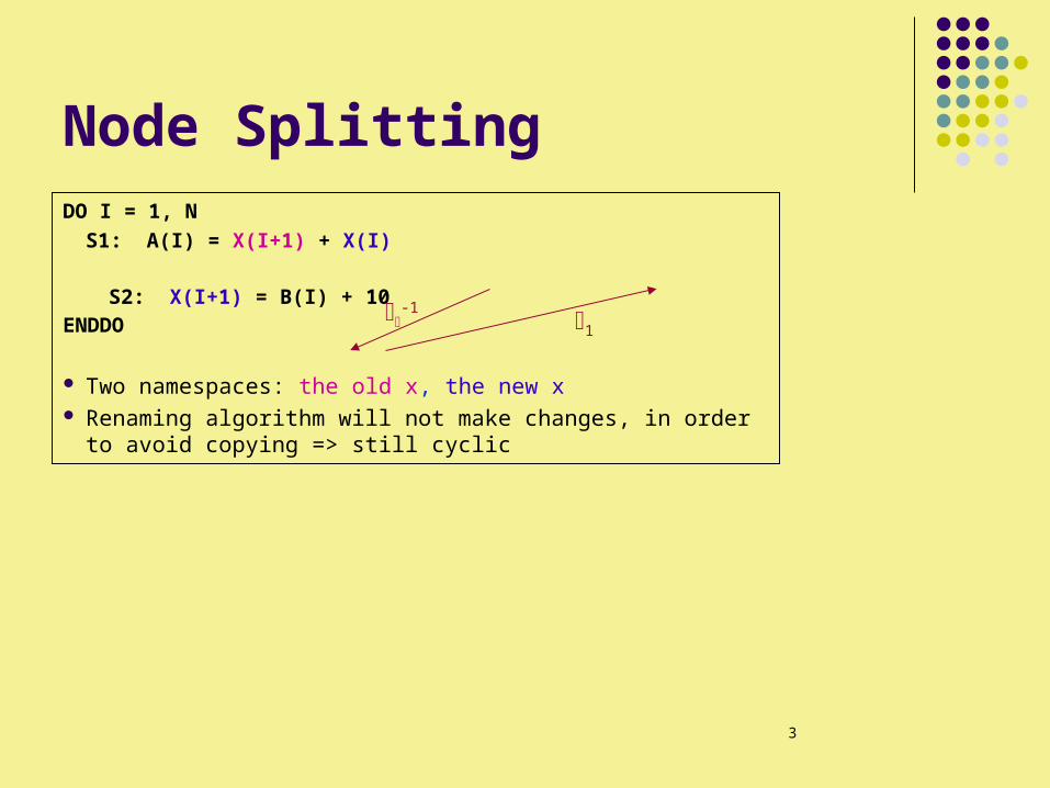
Node SplittingDO I = 1, N
S1: A(I) = X(I+1) + X(I)
S2: X(I+1) = B(I) + 10ENDDO
Two namespaces: the old x, the new x Renaming algorithm will not make changes, in order to avoid
copying => still cyclic
1
-1
4
Node Splitting - 2
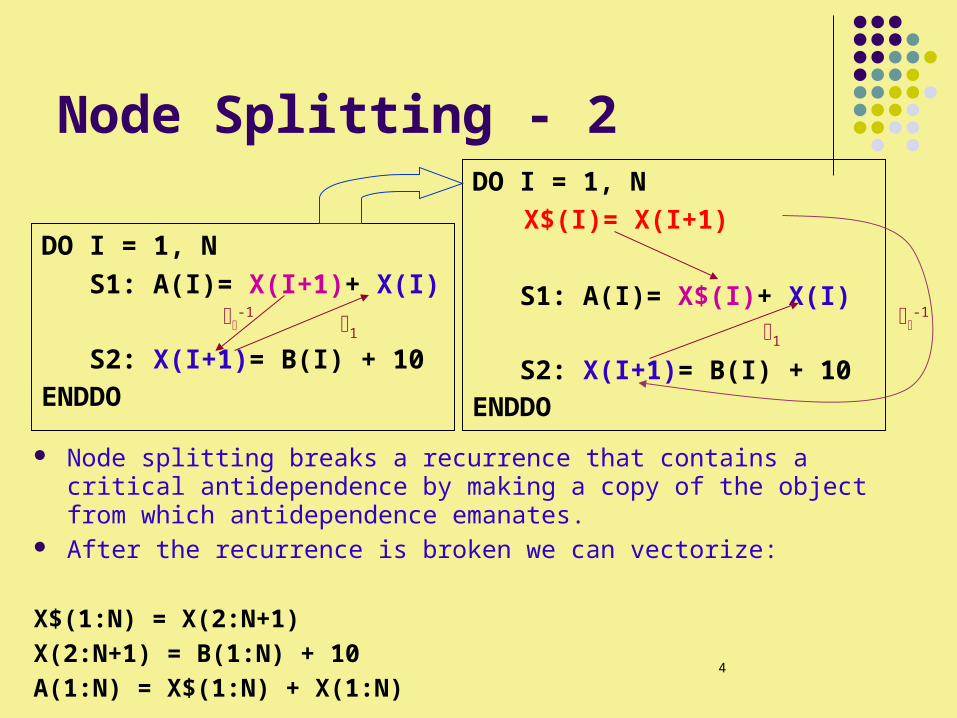
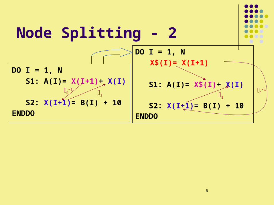
Node splitting breaks a recurrence that contains a critical antidependence by making a copy of the object from which antidependence emanates.
After the recurrence is broken we can vectorize:
X$(1:N) = X(2:N+1)X(2:N+1) = B(1:N) + 10A(1:N) = X$(1:N) + X(1:N)
DO I = 1, N S1: A(I)= X(I+1)+ X(I)
S2: X(I+1)= B(I) + 10ENDDO
1
-1
DO I = 1, N X$(I)= X(I+1)
S1: A(I)= X$(I)+ X(I)
S2: X(I+1)= B(I) + 10ENDDO
1
-1
5
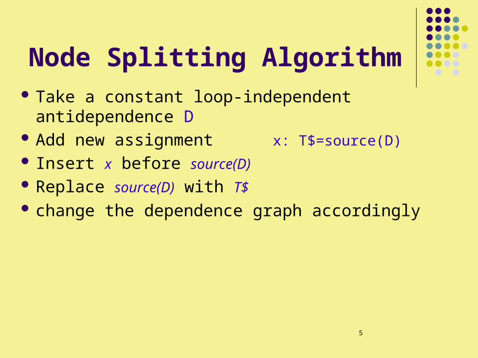
Node Splitting Algorithm Take a constant loop-independent antidependence D Add new assignment x: T$=source(D) Insert x before source(D) Replace source(D) with T$ change the dependence graph accordingly
6
Node Splitting - 2
DO I = 1, N S1: A(I)= X(I+1)+ X(I)
S2: X(I+1)= B(I) + 10ENDDO
1
-1
DO I = 1, N X$(I)= X(I+1)
S1: A(I)= X$(I)+ X(I)
S2: X(I+1)= B(I) + 10ENDDO
1
-1
7
Node Splitting: Profitability Node Splitting is not always profitable, i.e. does not always break
a recurrence.
To generate effective vectorization the antidependence we split must be “critical” to the recurrence.
For example…
8
Node Splitting: Profitability – Cont’d
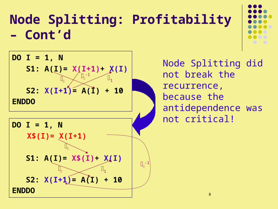
DO I = 1, N S1: A(I)= X(I+1)+ X(I)
S2: X(I+1)= A(I) + 10ENDDO
1
DO I = 1, N X$(I)= X(I+1)
S1: A(I)= X$(I)+ X(I)
S2: X(I+1)= A(I) + 10ENDDO
1
-1
-1
Node Splitting did not break the recurrence, because the antidependence was not critical!
9
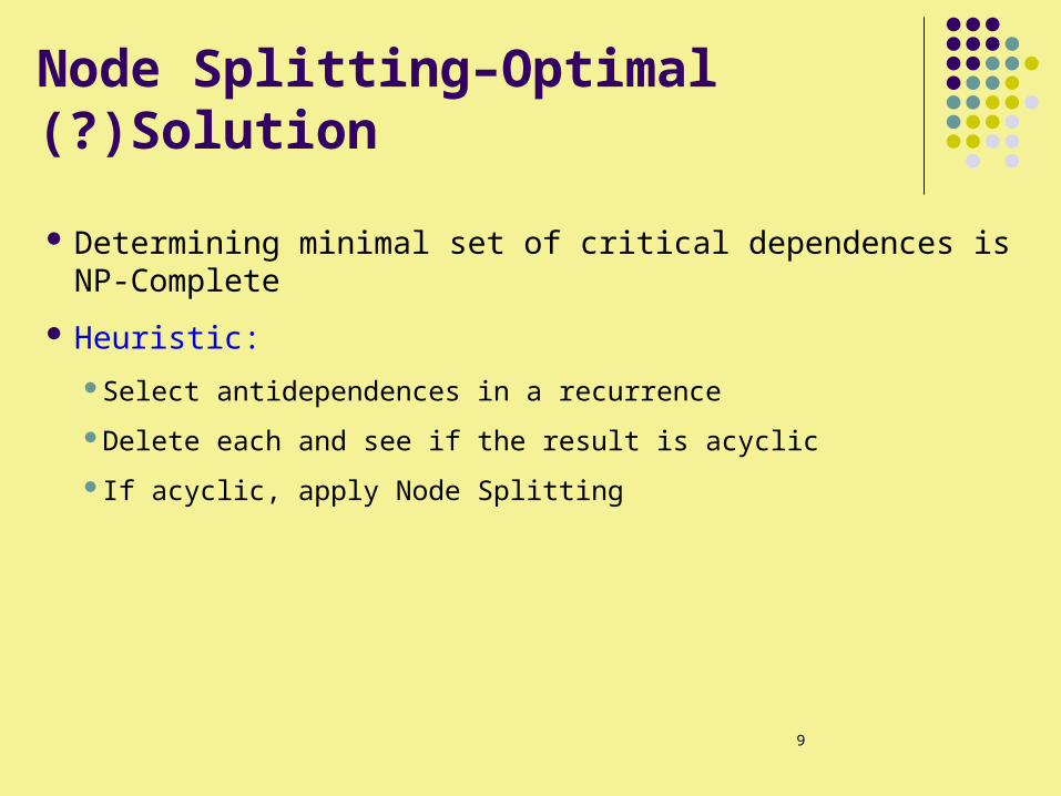
Node Splitting–Optimal Solution)?(
Determining minimal set of critical dependences is NP-Complete
Heuristic:
Select antidependences in a recurrence
Delete each and see if the result is acyclic
If acyclic, apply Node Splitting
10
Roadmap
Node Splitting Recognition of reductions Index-Set Splitting Run-Time Symbolic Resolution Loop Skewing Putting it all together Real Machines
11
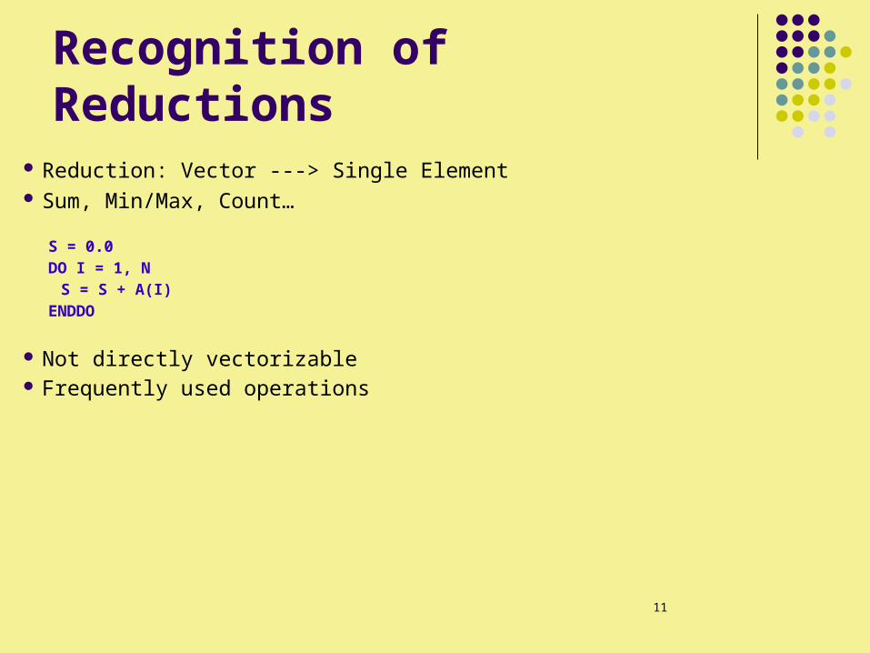
Recognition of Reductions Reduction: Vector ---> Single Element Sum, Min/Max, Count…
S = 0.0DO I = 1, N
S = S + A(I)ENDDO
Not directly vectorizable Frequently used operations
12
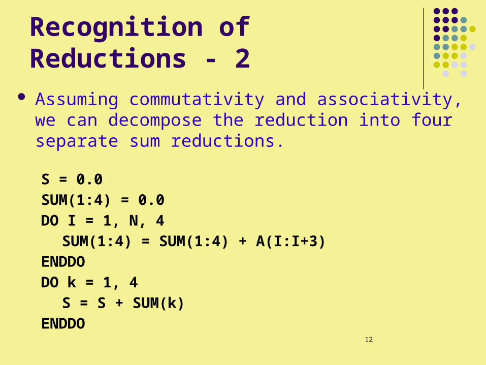
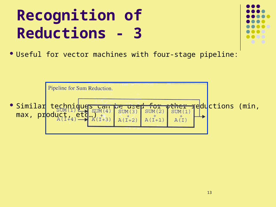
Recognition of Reductions - 2 Assuming commutativity and associativity, we can
decompose the reduction into four separate sum reductions.
S = 0.0SUM(1:4) = 0.0DO I = 1, N, 4 SUM(1:4) = SUM(1:4) + A(I:I+3)
ENDDODO k = 1, 4 S = S + SUM(k)
ENDDO
13
Recognition of Reductions - 3 Useful for vector machines with four-stage pipeline:
Similar techniques can be used for other reductions (min, max, product, etc…)
14
Recognition of Reductions - 4
Special reduction hardware and intrinsic functions (e.g. SUM() in Fortran 90) provide the fastest computation possible (for the specific machine).
The compiler should recognize the reduction-loop and replace it by the appropriate intrinsic call.
Example: s = SUM( A(1:N) )
15
Recognition of Reductions - 5
How can the compiler recognize reductions?
A Reduction has three properties:It reduces the elements of a vector to one elementNo use of Intermediate resultsIt operates on the vector and nothing else
These properties are easily determined from the dependence graph
16
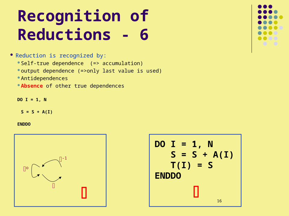
Recognition of Reductions - 6 Reduction is recognized by:
Self-true dependence (=> accumulation)output dependence (=>only last value is used)Antidependences Absence of other true dependences
DO I = 1, N
S = S + A(I) ENDDO
DO I = 1, N S = S + A(I) T(I) = SENDDO
o
-1
17
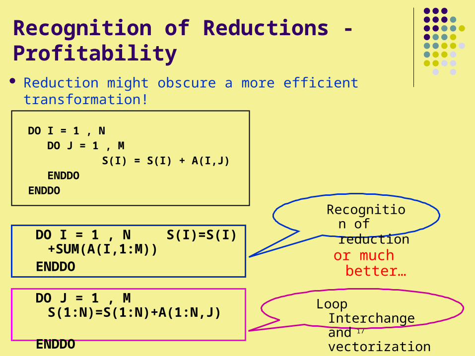
Recognition of Reductions - Profitability Reduction might obscure a more efficient transformation!
DO I = 1 , N DO J = 1 , M S(I) = S(I) + A(I,J) ENDDOENDDO
DO I = 1 , N S(I)=S(I)+SUM(A(I,1:M))
ENDDO
DO J = 1 , M S(1:N)=S(1:N)+A(1:N,J)
ENDDO
Recognition of reduction
Loop Interchange and vectorization
or much better…
18
Recognition of Reductions - Conclusion
It is important not to replace reductions too early, but rather to wait until all other options were considered!
19
Roadmap
Node Splitting Recognition of reductions Index-Set Splitting Run-Time Symbolic Resolution Loop Skewing Putting it all together Real Machines
20
Index-Set Splitting )“ISS”( Sometimes the loop contains a dependence
that holds for only partial range of iterations.
Full vectorization is impossible
Index-Set Splitting transformation subdivides the loop into different iteration ranges to achieve partial parallelization
Next we deal with:
Strong SIV, Weak Crossing SIV, Weak Zero SIV
21
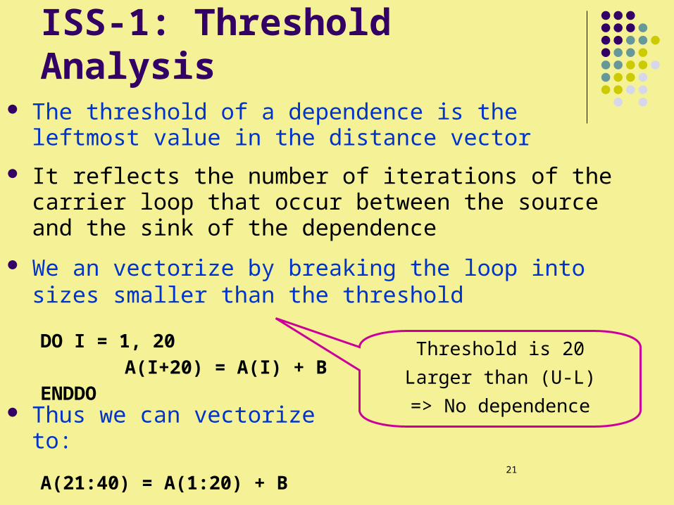
ISS-1: Threshold Analysis The threshold of a dependence is the leftmost value in the
distance vector
It reflects the number of iterations of the carrier loop that occur between the source and the sink of the dependence
We an vectorize by breaking the loop into sizes smaller than the threshold
DO I = 1, 20 A(I+20) = A(I) + B
ENDDOThreshold is 20
Larger than (U-L)
=> No dependence Thus we can vectorize to:
A(21:40) = A(1:20) + B
22
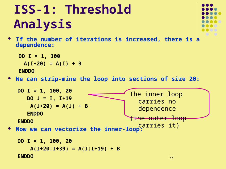
If the number of iterations is increased, there is a dependence:
DO I = 1, 100 A(I+20) = A(I) + B
ENDDO We can strip-mine the loop into sections of size 20:
DO I = 1, 100, 20 DO J = I, I+19
A(J+20) = A(J) + B ENDDO
ENDDO Now we can vectorize the inner-loop:
DO I = 1, 100, 20 A(I+20:I+39) = A(I:I+19) + B
ENDDO
ISS-1: Threshold Analysis
The inner loop carries no dependence
(the outer loop carries it)
23
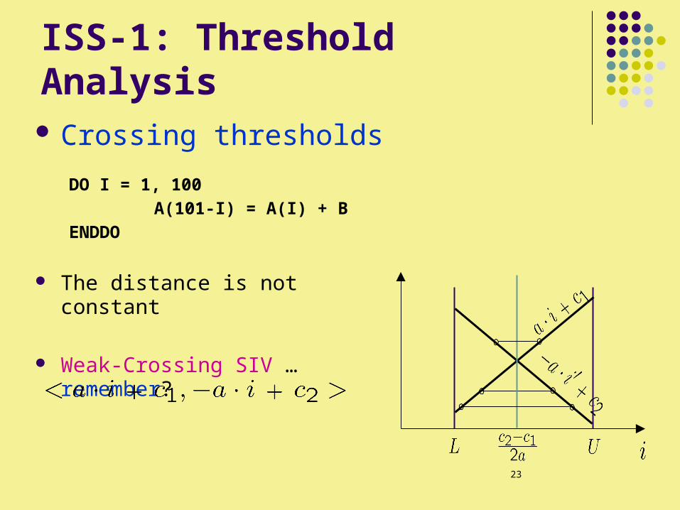
ISS-1: Threshold Analysis Crossing thresholds
DO I = 1, 100 A(101-I) = A(I) + B
ENDDO
The distance is not constant
Weak-Crossing SIV … remember?
24
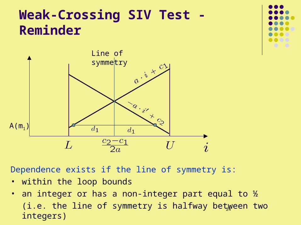
Weak-Crossing SIV Test - Reminder
Dependence exists if the line of symmetry is: • within the loop bounds • an integer or has a non-integer part equal to ½
(i.e. the line of symmetry is halfway between two integers)
Line of symmetry
A(m1)
25
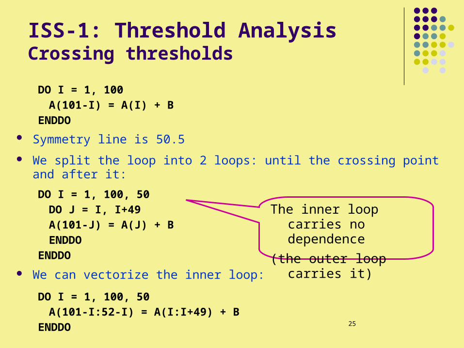
ISS-1: Threshold AnalysisCrossing thresholds
DO I = 1, 100 A(101-I) = A(I) + B
ENDDO
Symmetry line is 50.5
We split the loop into 2 loops: until the crossing point and after it:
DO I = 1, 100, 50DO J = I, I+49
A(101-J) = A(J) + BENDDO
ENDDO
We can vectorize the inner loop:
DO I = 1, 100, 50 A(101-I:52-I) = A(I:I+49) + B
ENDDO
The inner loop carries no dependence
(the outer loop carries it)
26
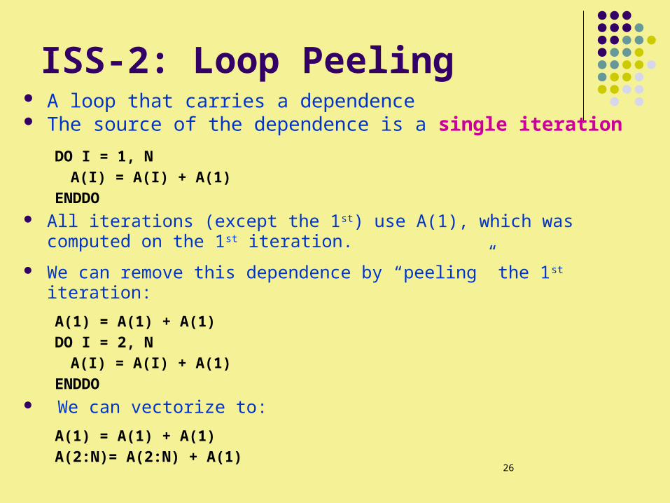
ISS-2: Loop Peeling A loop that carries a dependence The source of the dependence is a single iteration
DO I = 1, N A(I) = A(I) + A(1)
ENDDO All iterations (except the 1st) use A(1), which was computed on the 1st
iteration.
We can remove this dependence by “peeling” the 1st iteration:
A(1) = A(1) + A(1)DO I = 2, N
A(I) = A(I) + A(1)ENDDO
We can vectorize to:
A(1) = A(1) + A(1)A(2:N)= A(2:N) + A(1)
27
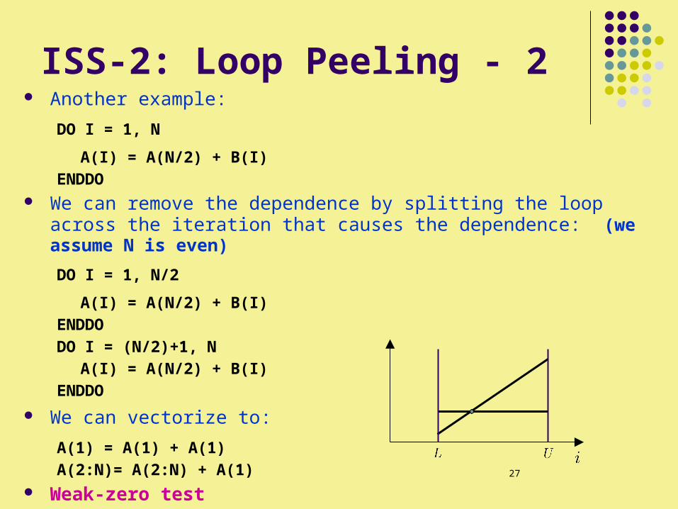
ISS-2: Loop Peeling - 2 Another example:
DO I = 1, N
A(I) = A(N/2) + B(I)ENDDO
We can remove the dependence by splitting the loop across the iteration that causes the dependence: )we assume N is even(
DO I = 1, N/2
A(I) = A(N/2) + B(I)ENDDODO I = (N/2)+1, N
A(I) = A(N/2) + B(I)ENDDO
We can vectorize to:
A(1) = A(1) + A(1)A(2:N)= A(2:N) + A(1)
Weak-zero test
28
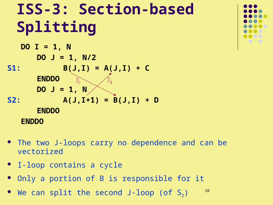
ISS-3: Section-based SplittingDO I = 1, N DO J = 1, N/2
S1: B(J,I) = A(J,I) + C ENDDO DO J = 1, N
S2: A(J,I+1) = B(J,I) + D ENDDO
ENDDO
The two J-loops carry no dependence and can be vectorized
I-loop contains a cycle
Only a portion of B is responsible for it
We can split the second J-loop (of S2)
1
29
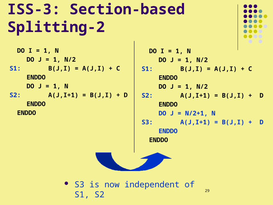
ISS-3: Section-based Splitting-2
DO I = 1, N DO J = 1, N/2
S1: B(J,I) = A(J,I) + C ENDDO DO J = 1, N
S2: A(J,I+1) = B(J,I) + D ENDDO
ENDDO
DO I = 1, N DO J = 1, N/2
S1: B(J,I) = A(J,I) + C ENDDO DO J = 1, N/2
S2: A(J,I+1) = B(J,I) + D ENDDO DO J = N/2+1, N
S3: A(J,I+1) = B(J,I) + D ENDDO
ENDDO
S3 is now independent of S1, S2
30
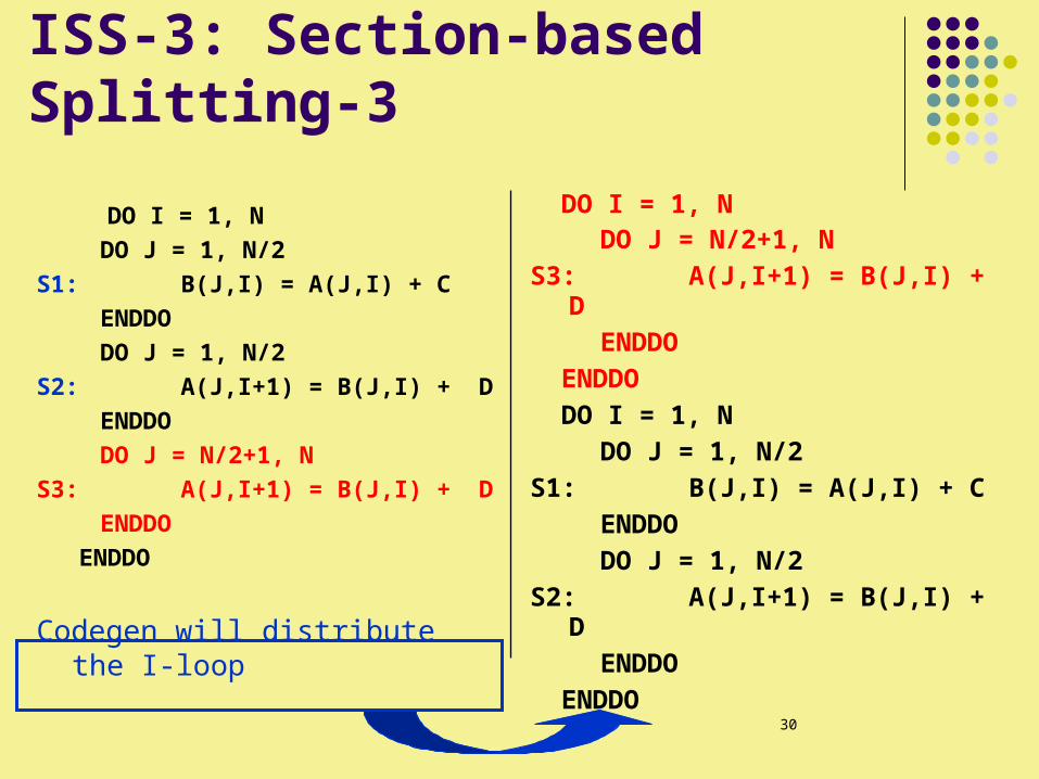
ISS-3: Section-based Splitting-3
DO I = 1, N DO J = N/2+1, N
S3: A(J,I+1) = B(J,I) + D ENDDO
ENDDO DO I = 1, N
DO J = 1, N/2 S1: B(J,I) = A(J,I) + C
ENDDO DO J = 1, N/2
S2: A(J,I+1) = B(J,I) + D ENDDO
ENDDO
DO I = 1, N DO J = 1, N/2
S1: B(J,I) = A(J,I) + C ENDDO DO J = 1, N/2
S2: A(J,I+1) = B(J,I) + D ENDDO DO J = N/2+1, N
S3: A(J,I+1) = B(J,I) + D ENDDO
ENDDO
Codegen will distribute the I-loop
31
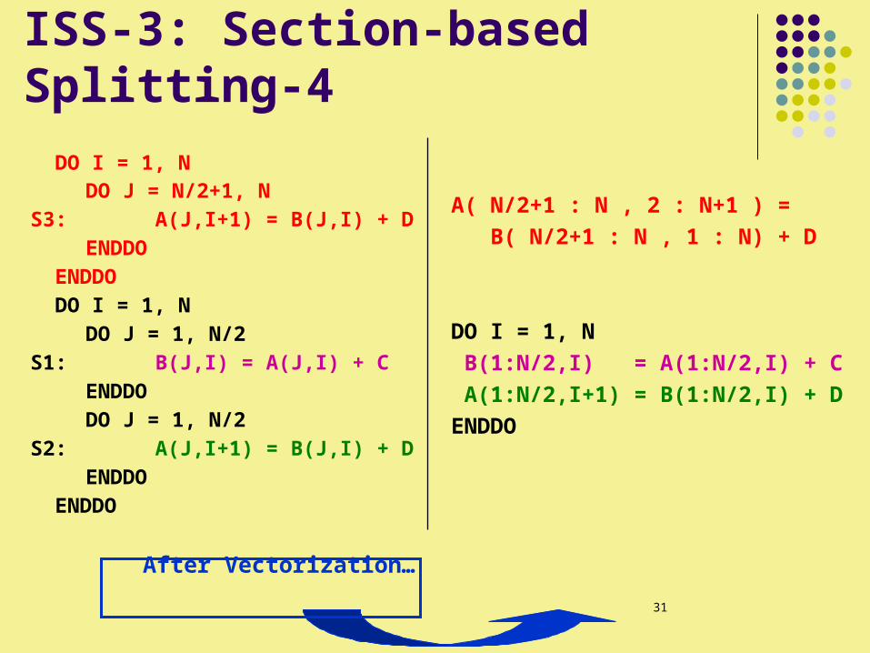
ISS-3: Section-based Splitting-4
DO I = 1, N DO J = N/2+1, N
S3: A(J,I+1) = B(J,I) + D ENDDO
ENDDO DO I = 1, N
DO J = 1, N/2 S1: B(J,I) = A(J,I) + C
ENDDO DO J = 1, N/2
S2: A(J,I+1) = B(J,I) + D ENDDO
ENDDO
After Vectorization…
A( N/2+1 : N , 2 : N+1 ) = B( N/2+1 : N , 1 : N) + D
DO I = 1, N B(1:N/2,I) = A(1:N/2,I) + C A(1:N/2,I+1) = B(1:N/2,I) + DENDDO
32
ISS-3: Section-based Splitting- Conclusion
Requires sophisticated analysis of array sections, flowing along dependence edges.
Probably too costly to be applied on all loop
Worthwhile in the context of procedure calls (chapter 11…)
33
Roadmap
Node Splitting Recognition of reductions Index-Set Splitting Run-Time Symbolic Resolution Loop Skewing Putting it all together Real Machines
34
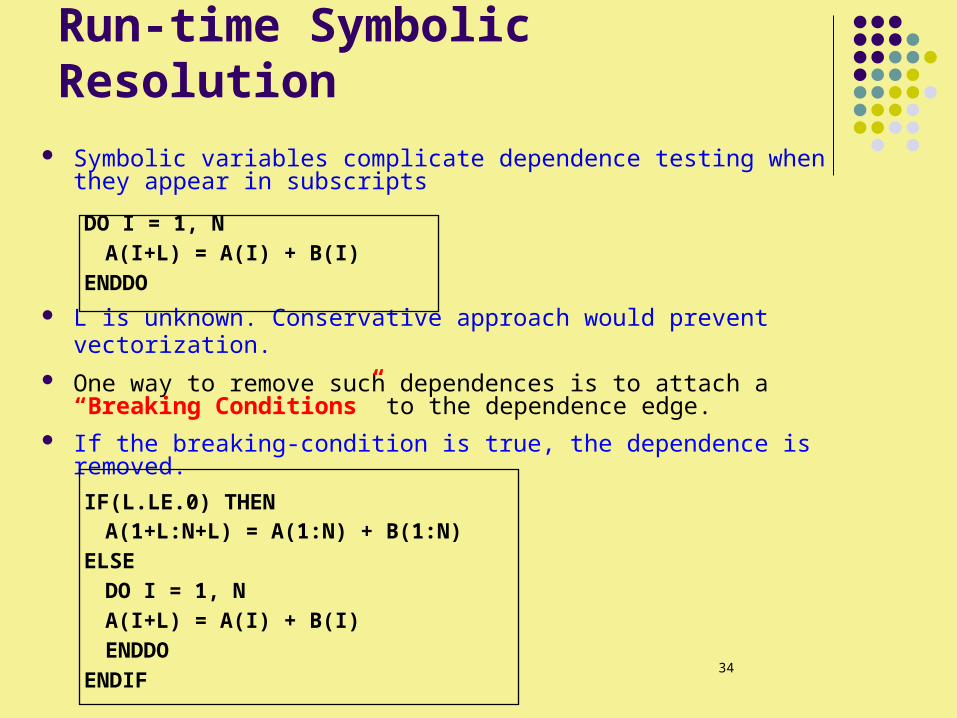
Run-time Symbolic Resolution Symbolic variables complicate dependence testing when they
appear in subscripts
DO I = 1, N A(I+L) = A(I) + B(I)
ENDDO L is unknown. Conservative approach would prevent vectorization. One way to remove such dependences is to attach a “Breaking
Conditions” to the dependence edge. If the breaking-condition is true, the dependence is removed.
IF(L.LE.0) THENA(1+L:N+L) = A(1:N) + B(1:N)
ELSEDO I = 1, N
A(I+L) = A(I) + B(I)ENDDO
ENDIF
35
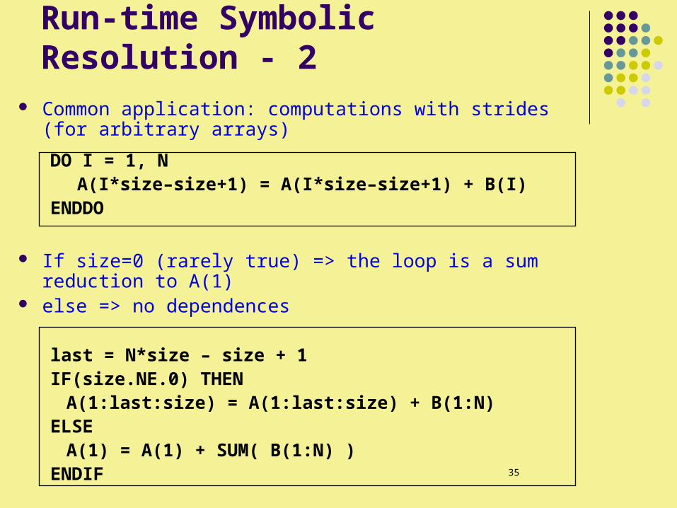
Run-time Symbolic Resolution - 2 Common application: computations with strides (for arbitrary
arrays)
DO I = 1, N A(I*size–size+1) = A(I*size–size+1) + B(I)
ENDDO
If size=0 (rarely true) => the loop is a sum reduction to A(1) else => no dependences
last = N*size – size + 1IF(size.NE.0) THENA(1:last:size) = A(1:last:size) + B(1:N)
ELSEA(1) = A(1) + SUM( B(1:N) )
ENDIF
36
Run-time Symbolic Resolution -Conclusion
A loop can contain several breaking condition
Impractical to handle all cases
Heuristic:
Identify when a critical dependence can be conditionally eliminated via a breaking condition
37
Roadmap
Node Splitting Recognition of reductions Index-Set Splitting Run-Time Symbolic Resolution Loop Skewing Putting it all together Real Machines
38
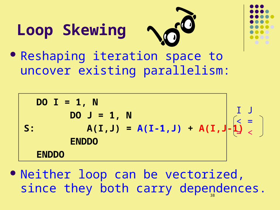
Loop Skewing
Reshaping iteration space to uncover existing parallelism:
DO I = 1, N DO J = 1, N
S: A(I,J) = A(I-1,J) + A(I,J-1) ENDDO
ENDDO
Neither loop can be vectorized, since they both carry dependences.
I J < = = <
39
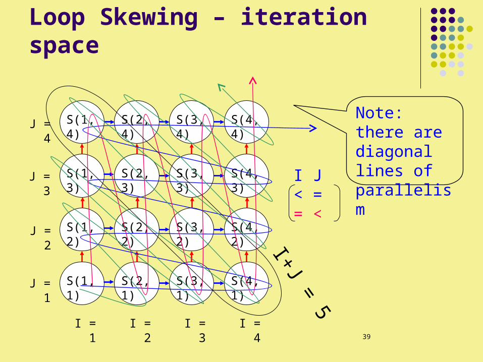
Loop Skewing – iteration space
I J < = = <
S(1,1)
S(1,3)
S(1,2)
S(1,4)
S(2,1)
S(2,3)
S(2,2)
S(2,4)
S(3,1)
S(3,3)
S(3,2)
S(3,4)
S(4,1)
S(4,3)
S(4,2)
S(4,4)
J = 1
J = 2
J = 3
J = 4
I = 1 I = 2 I = 3 I = 4
I+J = 5
Note: there are diagonal lines of parallelism
40
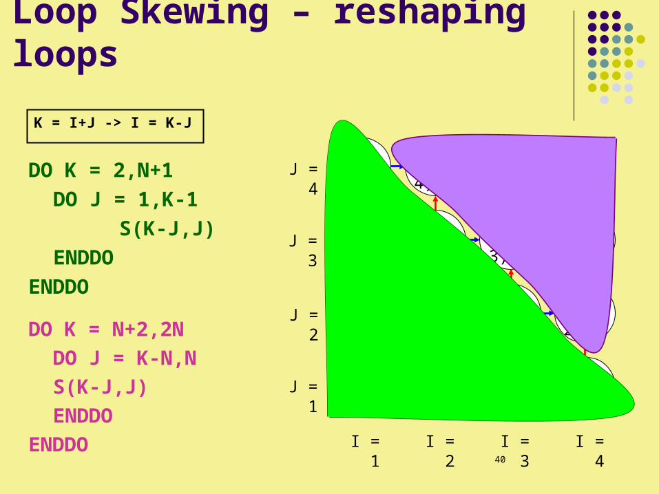
Loop Skewing – reshaping loops
S(1,1)
S(1,3)
S(1,2)
S(1,4)
S(2,1)
S(2,3)
S(2,2)
S(2,4)
S(3,1)
S(3,3)
S(3,2)
S(3,4)
S(4,1)
S(4,3)
S(4,2)
S(4,4)
J = 1
J = 2
J = 3
J = 4
I = 1 I = 2 I = 3 I = 4
DO K = 2,N+1
DO J = 1,K-1
S)K-J,J(
ENDDO
ENDDO
DO K = N+2,2N
DO J = K-N,N
S)K-J,J(
ENDDO
ENDDO
K = I+J -> I = K-J
41
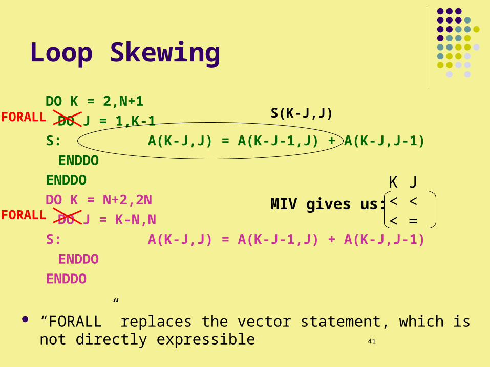
Loop Skewing
DO K = 2,N+1
DO J = 1,K-1
S: A)K-J,J( = A)K-J-1,J( + A)K-J,J-1(
ENDDO
ENDDO
DO K = N+2,2N
DO J = K-N,N
S: A)K-J,J( = A)K-J-1,J( + A)K-J,J-1(
ENDDO
ENDDO
“FORALL” replaces the vector statement, which is not directly expressible
K J < < < =
MIV gives us:
FORALL
FORALL
S)K-J,J(
42
Loop Skewing - conclusion
Disadvantages:Varying vector length
Not profitable if N is small
If vector startup time is more than speedup time, this
is not profitable
Vector bounds must be recomputed on each
iteration of the outer loop
Apply loop skewing if everything else fails
43
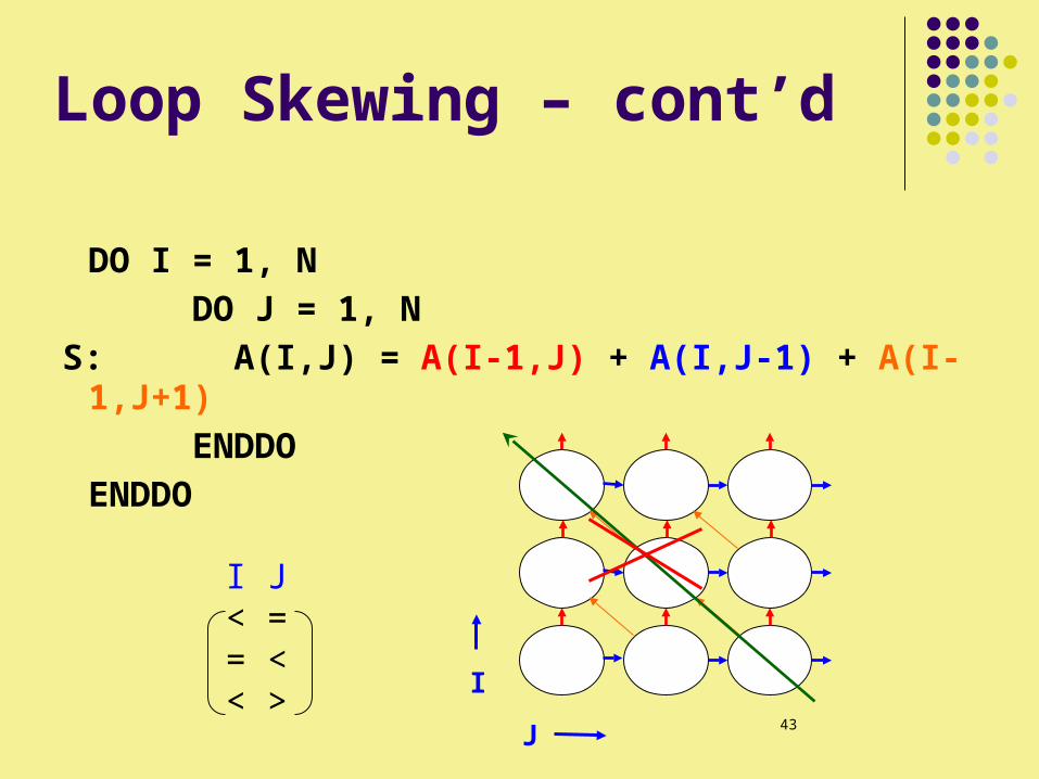
Loop Skewing – cont’d
DO I = 1, NDO J = 1, N
S: A(I,J) = A(I-1,J) + A(I,J-1) + A(I-1,J+1)
ENDDOENDDO
I J < = = << >
I
J
44
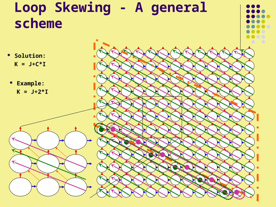
Loop Skewing - A general scheme
Solution:
K = J+C*I
Example:
K = J+2*I
45
Roadmap
Node Splitting Recognition of reductions Index-Set Splitting Run-Time Symbolic Resolution Loop Skewing Putting it all together Real Machines
46
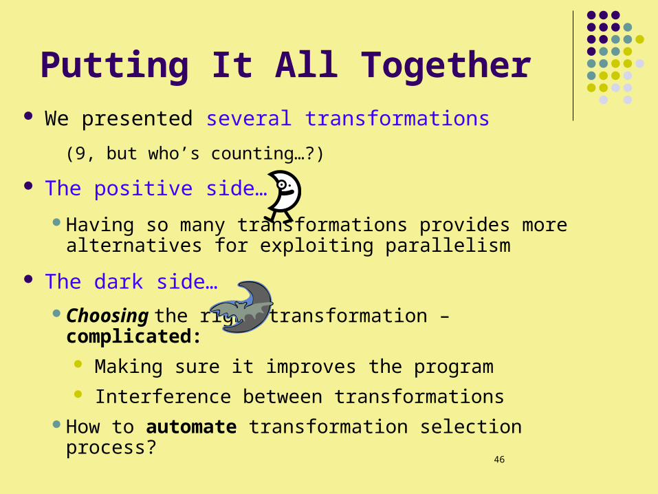
Putting It All Together We presented several transformations
(9, but who’s counting…?)
The positive side…
Having so many transformations provides more alternatives for exploiting parallelism
The dark side…
Choosing the right transformation – complicated: Making sure it improves the program Interference between transformations
How to automate transformation selection process?
47
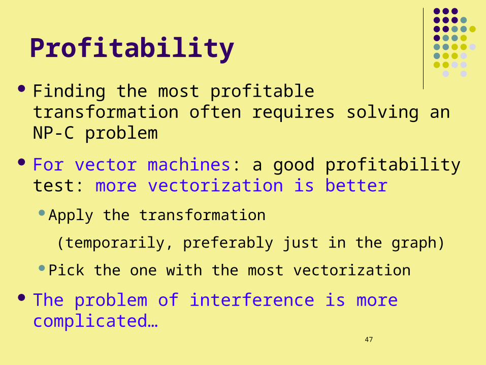
Profitability
Finding the most profitable transformation often requires solving an NP-C problem
For vector machines: a good profitability test: more vectorization is better
Apply the transformation
(temporarily, preferably just in the graph)
Pick the one with the most vectorization
The problem of interference is more complicated…
48
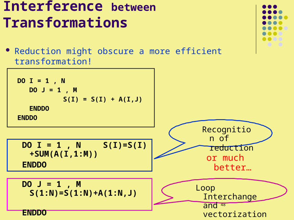
Interference between Transformations
Reduction might obscure a more efficient transformation!
DO I = 1 , N DO J = 1 , M S(I) = S(I) + A(I,J) ENDDOENDDO
DO I = 1 , N S(I)=S(I)+SUM(A(I,1:M))
ENDDO
DO J = 1 , M S(1:N)=S(1:N)+A(1:N,J)
ENDDO
Recognition of reduction
Loop Interchange and vectorization
or much better…
49
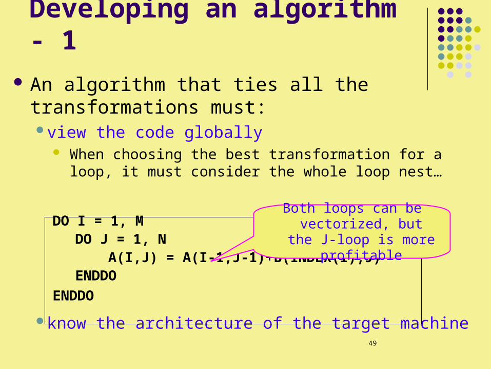
Developing an algorithm - 1
An algorithm that ties all the transformations must:view the code globally
When choosing the best transformation for a loop, it must consider the whole loop nest…
DO I = 1, MDO J = 1, N A(I,J) = A(I-1,J-1)+B(INDEX(I),J)ENDDO
ENDDO
know the architecture of the target machine
Both loops can be vectorized, but the J-loop
is more profitable
50
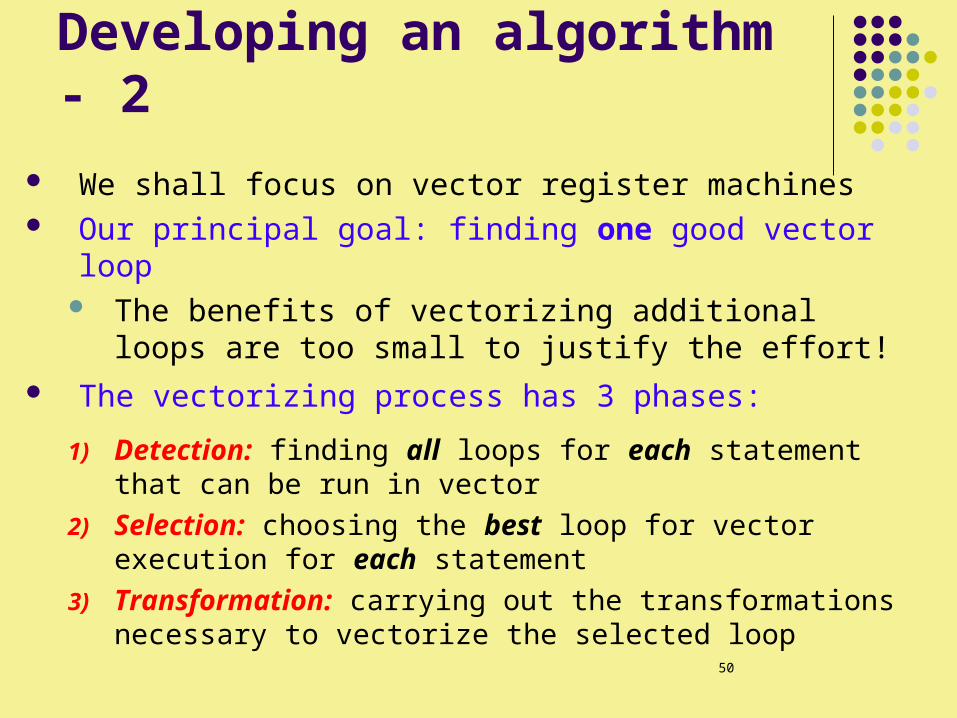
Developing an algorithm - 2
We shall focus on vector register machines Our principal goal: finding one good vector loop
The benefits of vectorizing additional loops are too small to justify the effort!
The vectorizing process has 3 phases:
1) Detection: finding all loops for each statement that can be run in vector
2) Selection: choosing the best loop for vector execution for each statement
3) Transformation: carrying out the transformations necessary to vectorize the selected loop
51
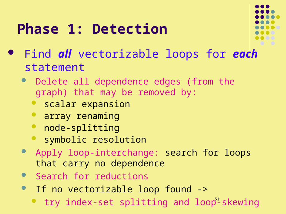
Phase 1: Detection
Find all vectorizable loops for each statement Delete all dependence edges (from the graph) that may
be removed by: scalar expansion array renaming node-splitting symbolic resolution
Apply loop-interchange: search for loops that carry no dependence
Search for reductions If no vectorizable loop found ->
try index-set splitting and loop-skewing
52
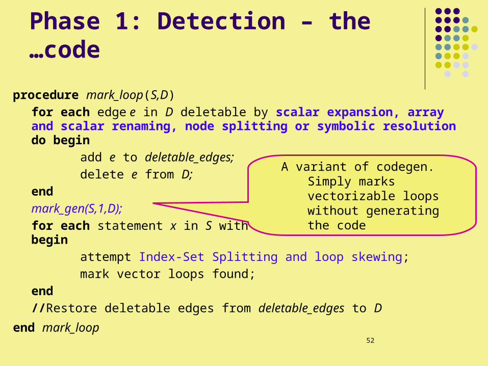
Phase 1: Detection – the code…
procedure mark_loop(S,D)for each edge e in D deletable by scalar expansion, array and scalar renaming, node splitting or symbolic resolution do begin
add e to deletable_edges;delete e from D;
endmark_gen(S,1,D);for each statement x in S with no vector loop marked do begin
attempt Index-Set Splitting and loop skewing; mark vector loops found;
end//Restore deletable edges from deletable_edges to D
end mark_loop
A variant of codegen. Simply marks vectorizable loops without generating the code
53
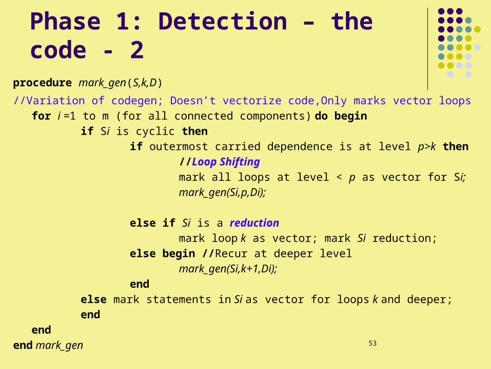
Phase 1: Detection – the code - 2procedure mark_gen(S,k,D)
//Variation of codegen; Doesn’t vectorize code,Only marks vector loopsfor i =1 to m (for all connected components) do begin
if Si is cyclic then if outermost carried dependence is at level p>k then
//Loop Shifting mark all loops at level < p as vector for Si;mark_gen(Si,p,Di);
else if Si is a reduction mark loop k as vector; mark Si reduction;
else begin //Recur at deeper levelmark_gen(Si,k+1,Di);
endelse mark statements in Si as vector for loops k and deeper;end
endend mark_gen
54
Phase 2: Selection
Choose the best vectorizable loop for each statement
Highly machine dependent Requires global analysis The most difficult phase to implement
55
Phase 3: Transformation
carry out the transformations necessary to vectorize the selected-best-loop:
Invoke codegen on the original graph
Whenever reaching a “best vectorizable loop” that does not directly vectorize:
perform transformation
(again, loop-skewing and index-set splitting are the last resort)
56
Phase 3: Transformation – the code
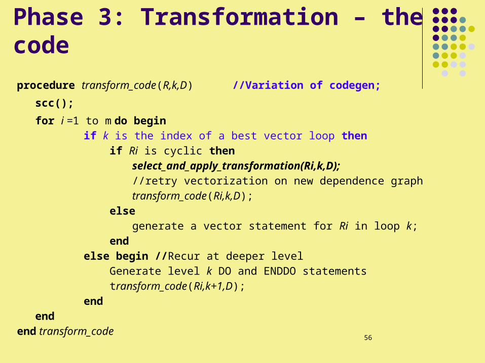
procedure transform_code(R,k,D) //Variation of codegen;
scc();
for i =1 to m do beginif k is the index of a best vector loop then if Ri is cyclic then
select_and_apply_transformation(Ri,k,D);//retry vectorization on new dependence graphtransform_code(Ri,k,D);
else generate a vector statement for Ri in loop k;
endelse begin //Recur at deeper level Generate level k DO and ENDDO statements transform_code(Ri,k+1,D);end
endend transform_code
57
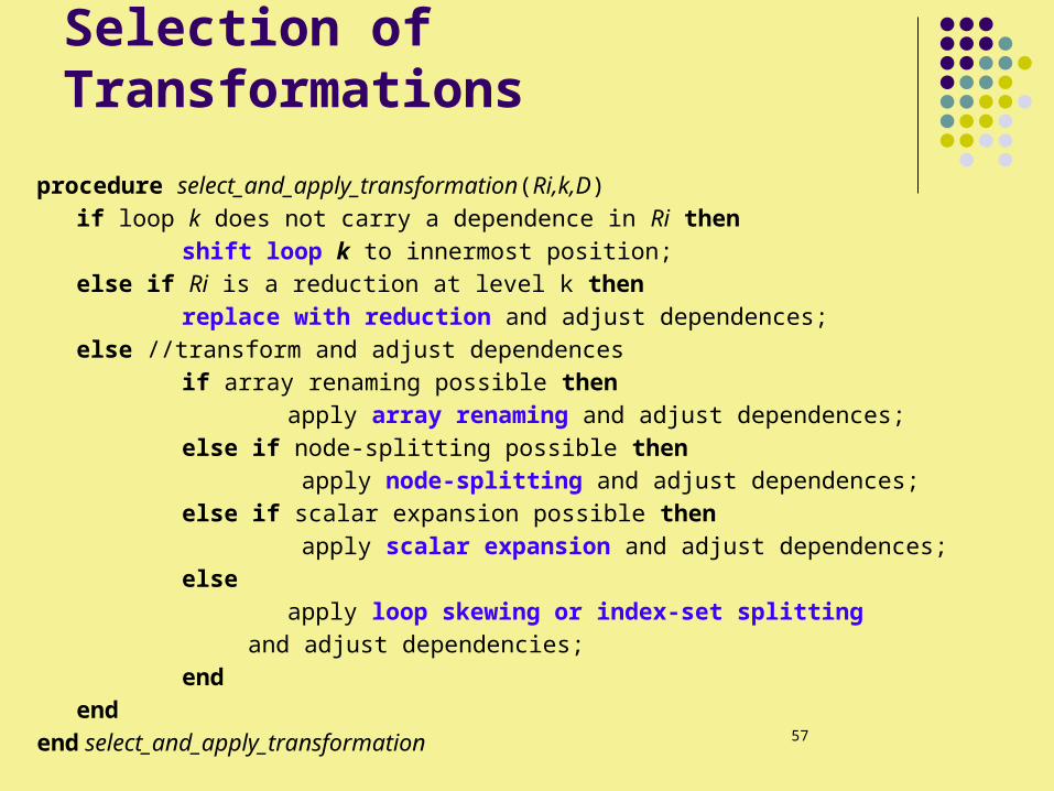
Selection of Transformations
procedure select_and_apply_transformation(Ri,k,D) if loop k does not carry a dependence in Ri then
shift loop k to innermost position;else if Ri is a reduction at level k then
replace with reduction and adjust dependences;else //transform and adjust dependences
if array renaming possible thenapply array renaming and adjust dependences;
else if node-splitting possible then apply node-splitting and adjust dependences;
else if scalar expansion possible then apply scalar expansion and adjust dependences;
else apply loop skewing or index-set splitting
and adjust dependencies;end
endend select_and_apply_transformation
58
Roadmap
Node Splitting Recognition of reductions Index-Set Splitting Run-Time Symbolic Resolution Loop Skewing Putting it all together Real Machines
59
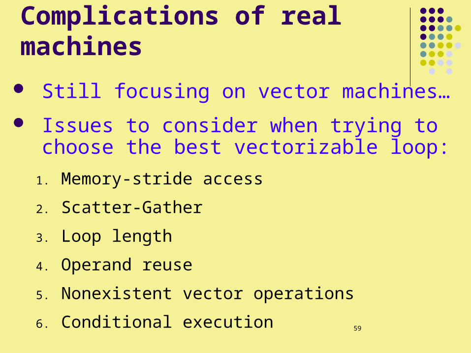
Complications of real machines
Still focusing on vector machines…
Issues to consider when trying to choose the best vectorizable loop:
1. Memory-stride access
2. Scatter-Gather
3. Loop length
4. Operand reuse
5. Nonexistent vector operations
6. Conditional execution
60
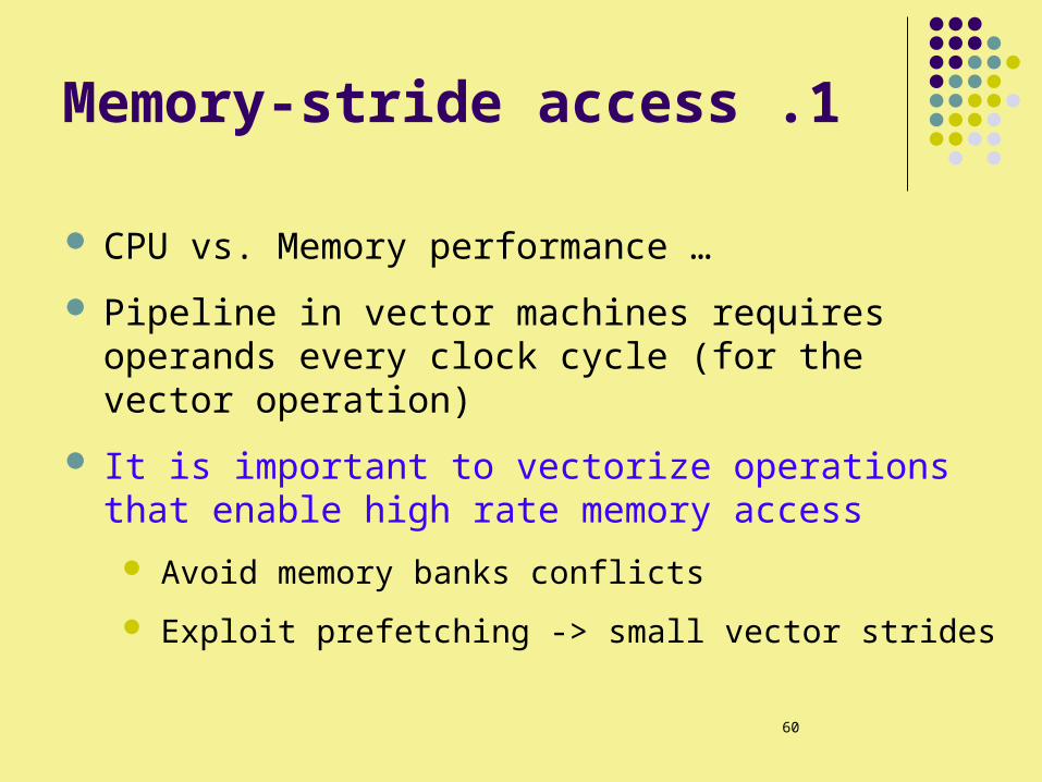
1 .Memory-stride access
CPU vs. Memory performance …
Pipeline in vector machines requires operands every clock cycle (for the vector operation)
It is important to vectorize operations that enable high rate memory access
Avoid memory banks conflicts
Exploit prefetching -> small vector strides
61
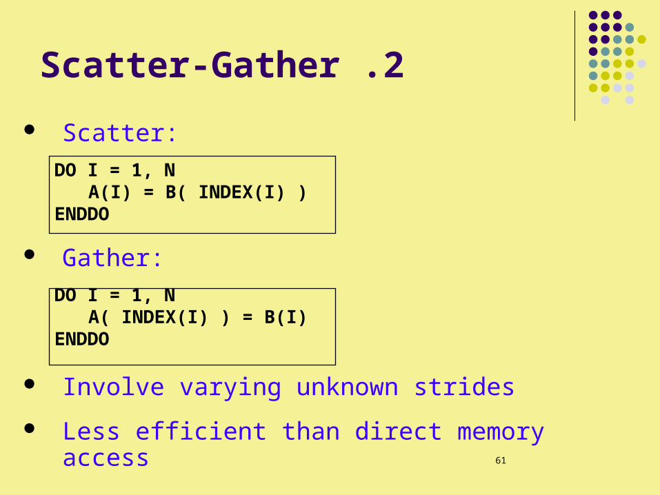
2 .Scatter-Gather
Scatter:
DO I = 1, NA(I) = B( INDEX(I) )
ENDDO
Gather:
DO I = 1, NA( INDEX(I) ) = B(I)
ENDDO
Involve varying unknown strides
Less efficient than direct memory access
62
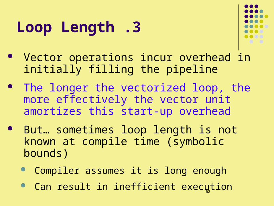
3 .Loop Length
Vector operations incur overhead in initially filling the pipeline
The longer the vectorized loop, the more effectively the vector unit amortizes this start-up overhead
But… sometimes loop length is not known at compile time (symbolic bounds)
Compiler assumes it is long enough
Can result in inefficient execution
63
4 .Operand reuse
Prefer vector loops where operands are reused from registers
Operand reuse minimizes memory access
64
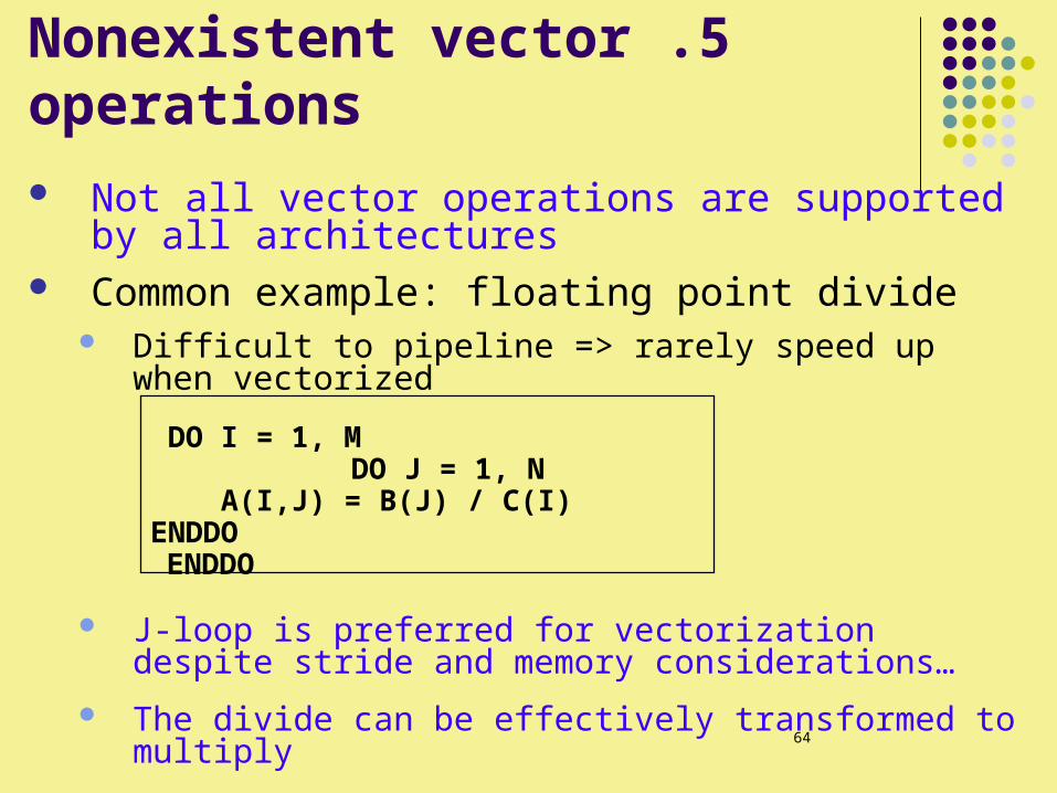
5 .Nonexistent vector operations
Not all vector operations are supported by all architectures
Common example: floating point divide Difficult to pipeline => rarely speed up when vectorized
DO I = 1, M DO J = 1, N
A(I,J) = B(J) / C(I) ENDDO
ENDDO
J-loop is preferred for vectorization despite stride and memory considerations…
The divide can be effectively transformed to multiply
65
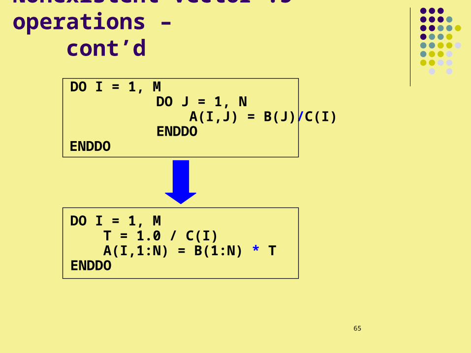
5 .Nonexistent vector operations – cont’d
DO I = 1, M DO J = 1, N
A(I,J) = B(J)/C(I) ENDDO
ENDDO
DO I = 1, M T = 1.0 / C(I) A(I,1:N) = B(1:N) * T ENDDO
66
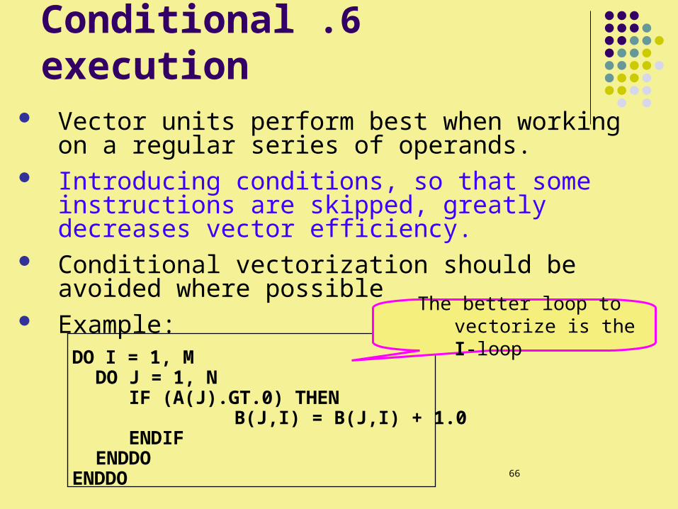
6 .Conditional execution Vector units perform best when working on a
regular series of operands. Introducing conditions, so that some instructions
are skipped, greatly decreases vector efficiency. Conditional vectorization should be avoided where
possible Example:
DO I = 1, M DO J = 1, N IF (A(J).GT.0) THEN B(J,I) = B(J,I) + 1.0 ENDIF ENDDO
ENDDO
The better loop to vectorize is the I-loop
67
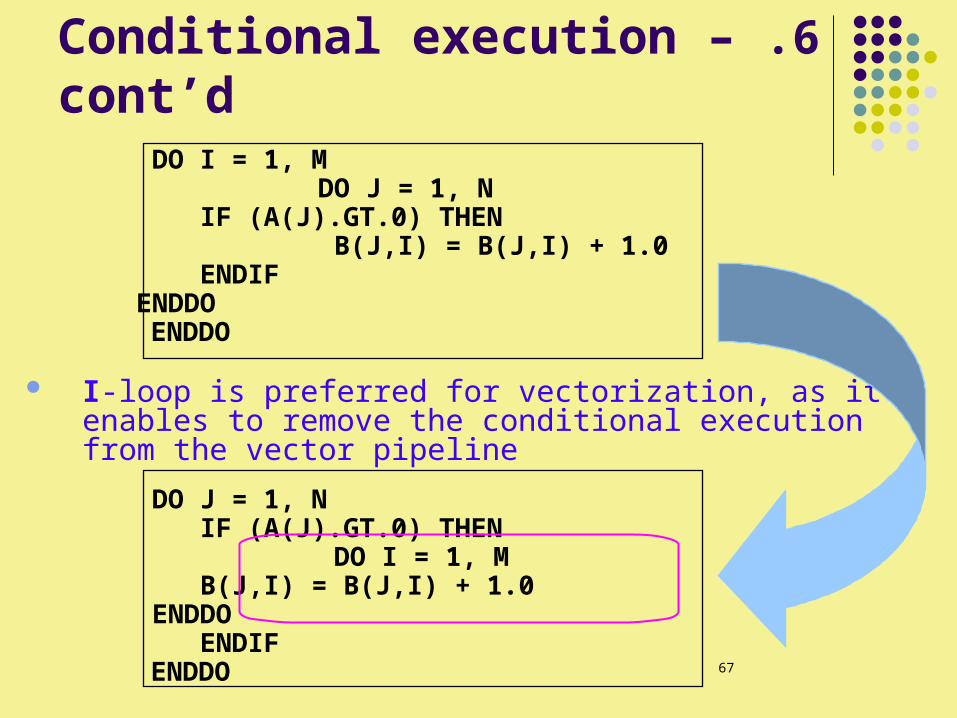
6 .Conditional execution – cont’d DO I = 1, M DO J = 1, N
IF (A(J).GT.0) THEN B(J,I) = B(J,I) + 1.0 ENDIF ENDDO
ENDDO
I-loop is preferred for vectorization, as it enables to remove the conditional execution from the vector pipeline
DO J = 1, N IF (A(J).GT.0) THEN
DO I = 1, M B(J,I) = B(J,I) + 1.0 ENDDO
ENDIF ENDDO
68
Node Splitting
Recognition of reductions
Index-Set Splitting Run-Time Symbolic
Resolution Loop Skewing Putting it all together Real Machines END
Roadmap