Ensemble Learning

Ensemble Learning

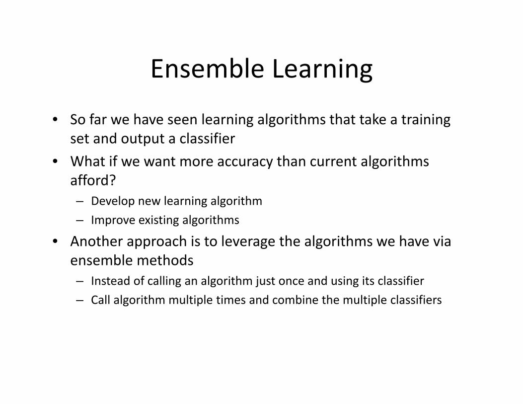
• So far we have seen learning algorithms that take a training set and output a classifier

• What if we want more accuracy than current algorithms afford?– Develop new learning algorithm– Improve existing algorithms

• Another approach is to leverage the algorithms we have via ensemble methods– Instead of calling an algorithm just once and using its classifier– Call algorithm multiple times and combine the multiple classifiers

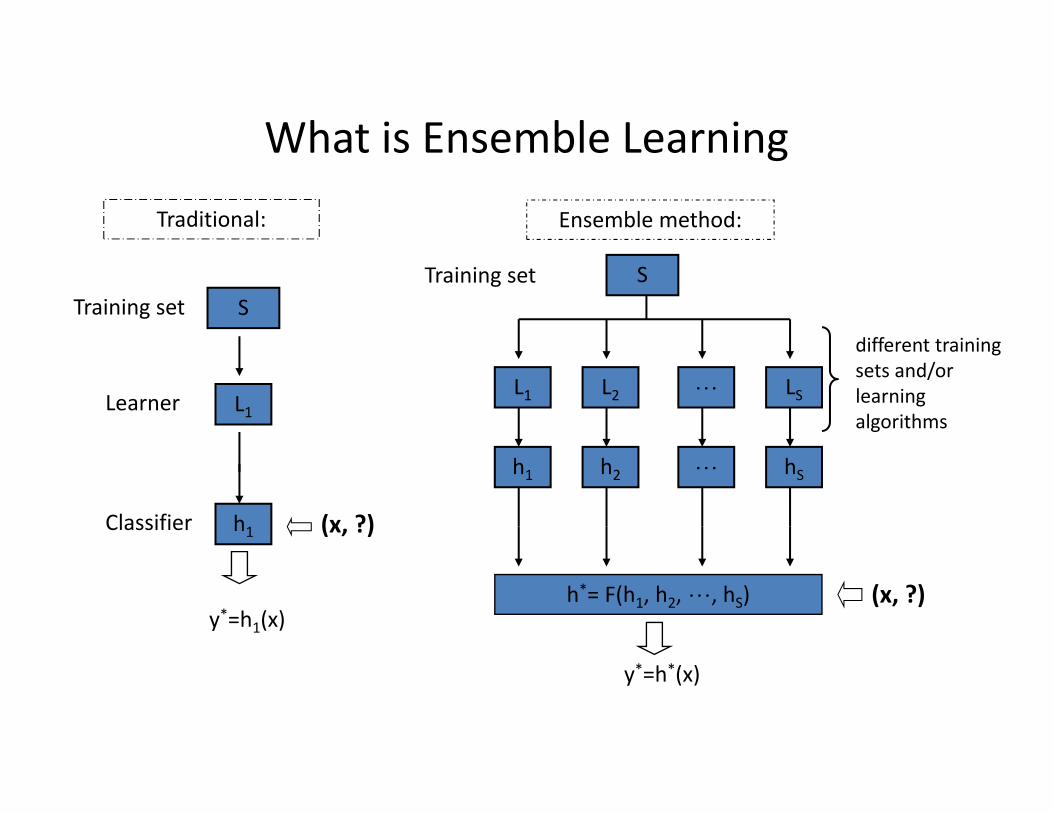
What is Ensemble Learning

S

L2 LS

h2 hS

different training sets and/or learning algorithms

Ensemble method:

h*= F(h1, h2, , hS) (x, ?)

y*=h*(x)

L1

h1

L1

Traditional:

S

h1 (x, ?)

y*=h1(x)

Training set

Learner

Classifier

Training set

Ensemble Learning

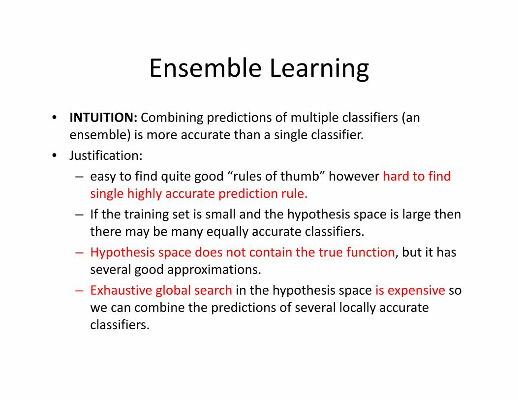
• INTUITION: Combining predictions of multiple classifiers (an ensemble) is more accurate than a single classifier.

• Justification:– easy to find quite good “rules of thumb” however hard to find 

single highly accurate prediction rule.– If the training set is small and the hypothesis space is large then 

there may be many equally accurate classifiers.– Hypothesis space does not contain the true function, but it has 

several good approximations.– Exhaustive global search in the hypothesis space is expensive so 

we can combine the predictions of several locally accurate classifiers.

How to generate ensemble?

• There are a variety of methods developed• We will look at two of them:

– Bagging– Boosting (Adaboost: adaptive boosting)

• Both of these methods takes a single learning algorithm (we will call it the base learner) and use it multiple times to generate multiple classifiers

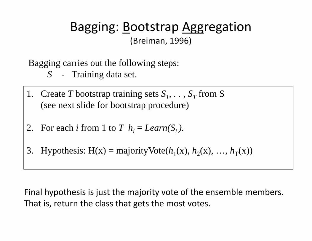
1. Create T bootstrap training sets S1, . . , ST from S(see next slide for bootstrap procedure)

2. For each i from 1 to T hi = Learn(Si ).

3. Hypothesis: H(x) = majorityVote(h1(x), h2(x), …, hT(x))

Bagging carries out the following steps:S - Training data set.

Bagging: Bootstrap Aggregation(Breiman, 1996)

Final hypothesis is just the majority vote of the ensemble members. That is, return the class that gets the most votes.

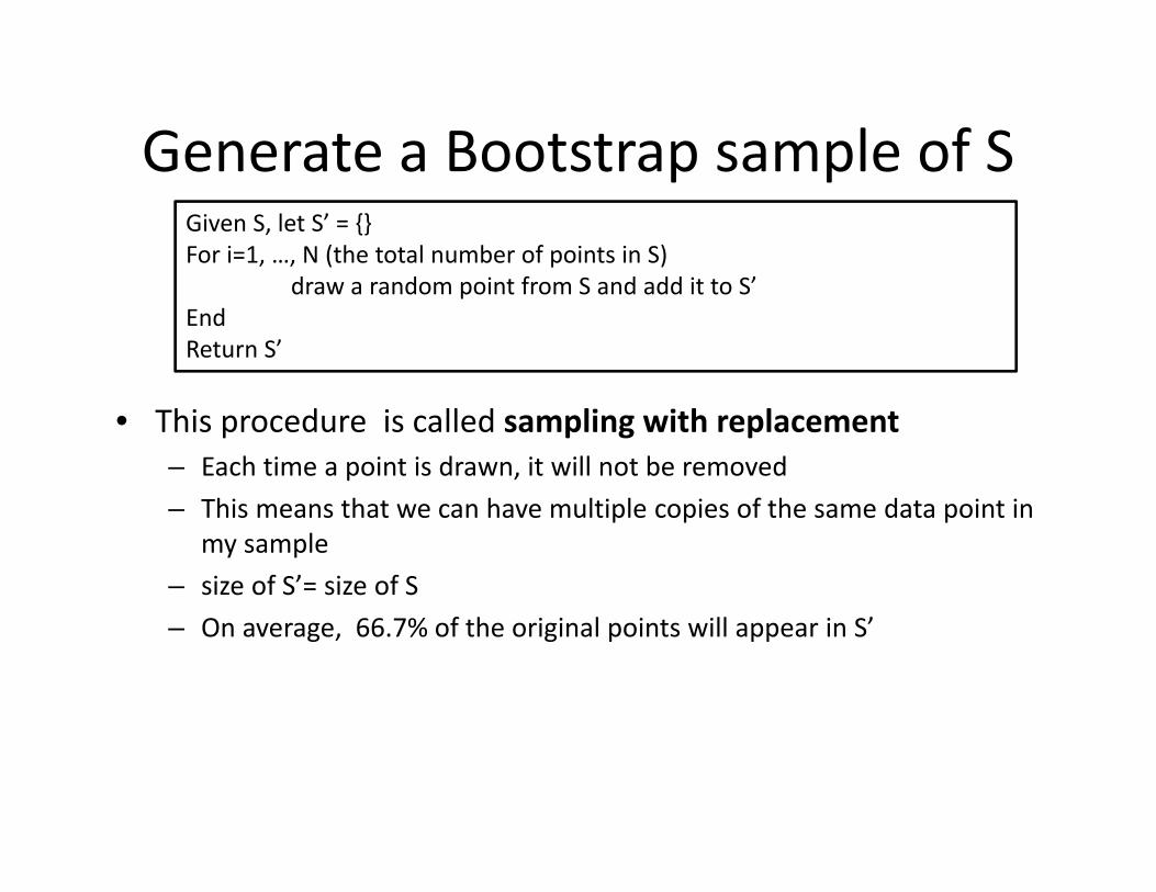
Generate a Bootstrap sample of S

• This procedure  is called sampling with replacement– Each time a point is drawn, it will not be removed– This means that we can have multiple copies of the same data point in 

my sample– size of S’= size of S– On average,  66.7% of the original points will appear in S’

Given S, let S’ = {}For i=1, …, N (the total number of points in S)

draw a random point from S and add it to S’EndReturn S’

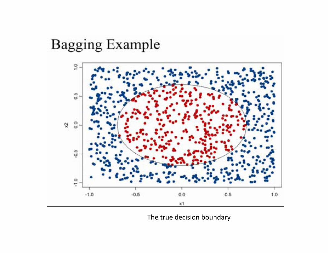
The true decision boundary

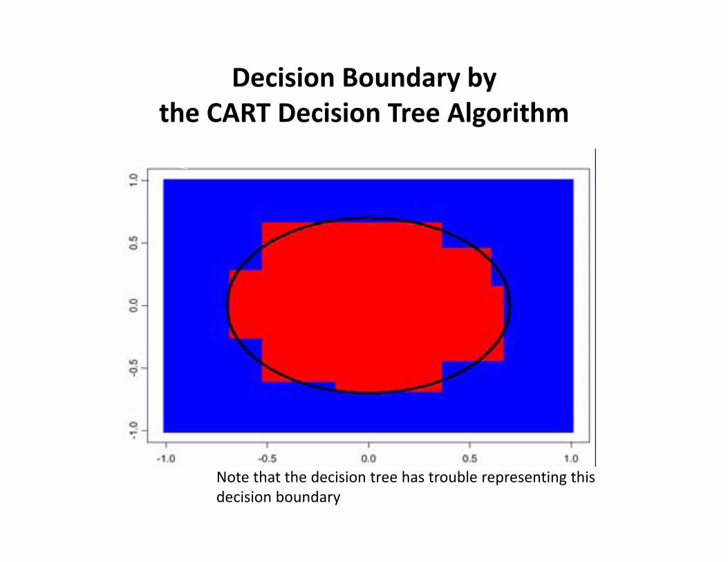
Decision Boundary by the CART Decision Tree Algorithm

Note that the decision tree has trouble representing this decision boundary

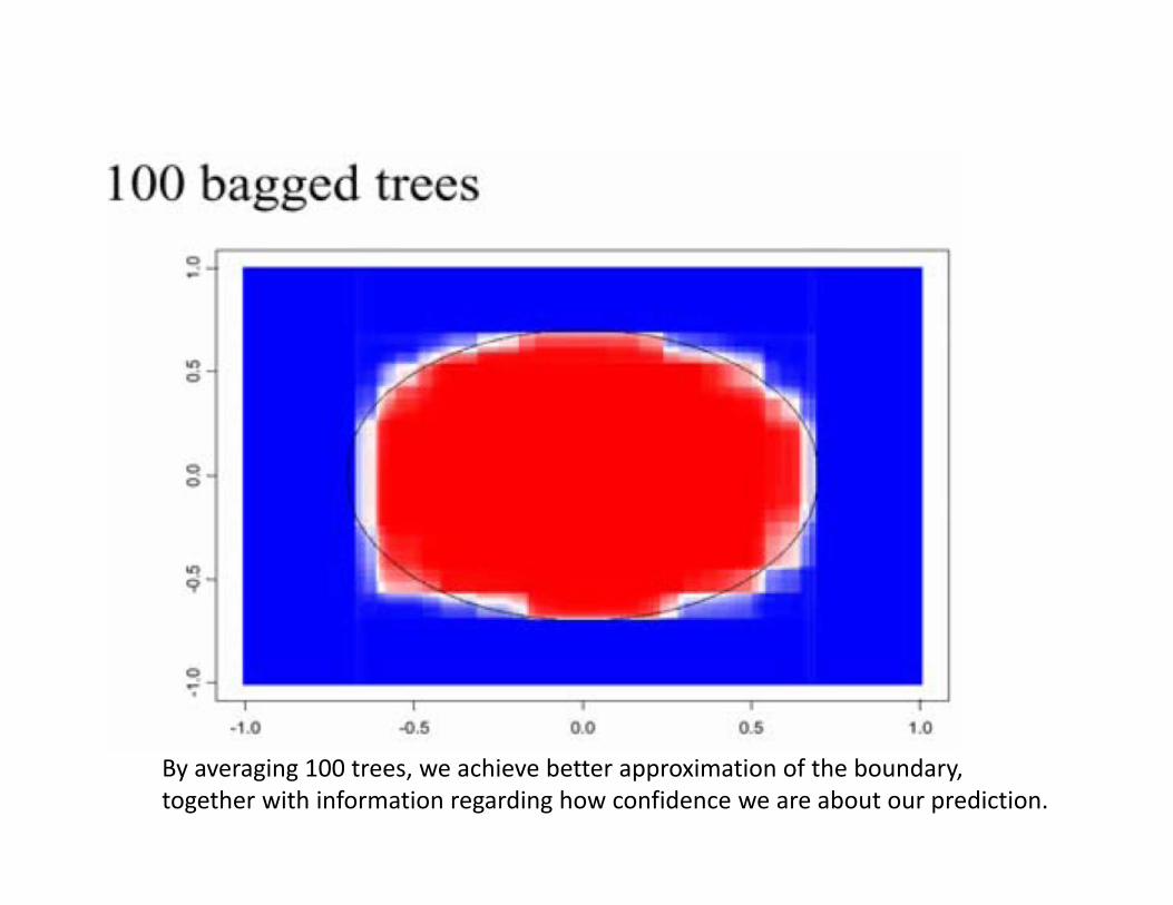
By averaging 100 trees, we achieve better approximation of the boundary, together with information regarding how confidence we are about our prediction.

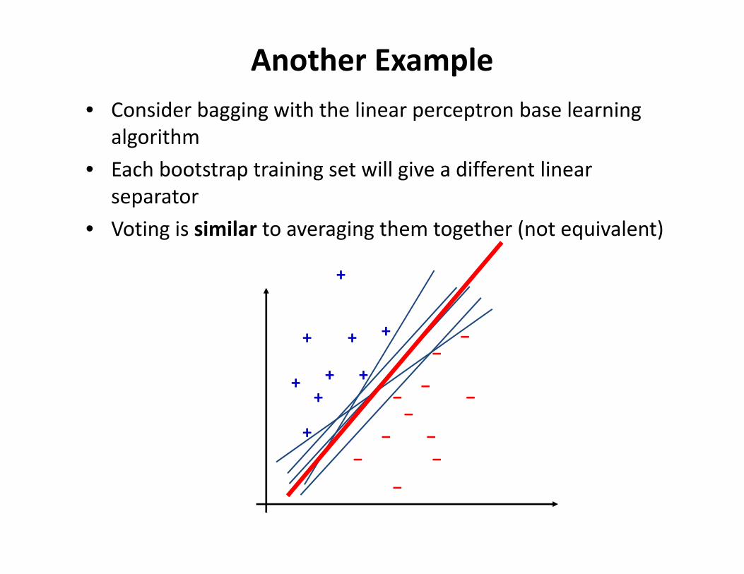
Another Example• Consider bagging with the linear perceptron base learning 

algorithm• Each bootstrap training set will give a different linear 

separator• Voting is similar to averaging them together (not equivalent)

+ +

+

+

+

+ ++

+

−−

−

−

− −

−

−

−−

−

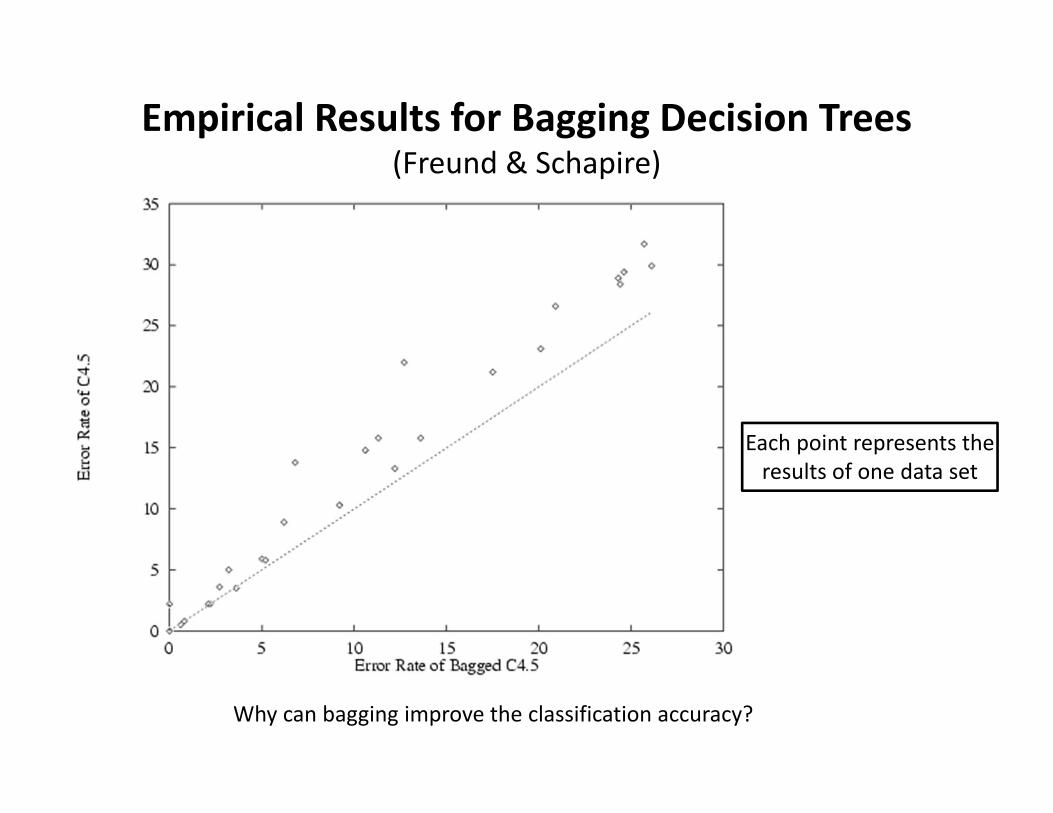
Empirical Results for Bagging Decision Trees(Freund & Schapire)

Each point represents the results of one data set

Why can bagging improve the classification accuracy?

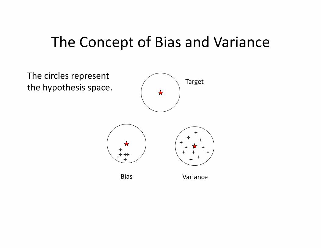
The Concept of Bias and Variance

Bias Variance

TargetThe circles represent the hypothesis space.

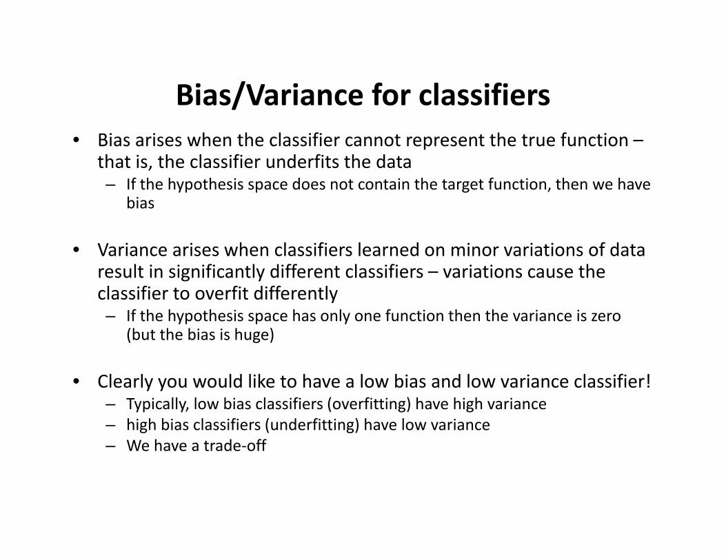
Bias/Variance for classifiers• Bias arises when the classifier cannot represent the true function –

that is, the classifier underfits the data– If the hypothesis space does not contain the target function, then we have 

bias

• Variance arises when classifiers learned on minor variations of data result in significantly different classifiers – variations cause the classifier to overfit differently– If the hypothesis space has only one function then the variance is zero

(but the bias is huge)

• Clearly you would like to have a low bias and low variance classifier!– Typically, low bias classifiers (overfitting) have high variance– high bias classifiers (underfitting) have low variance– We have a trade‐off

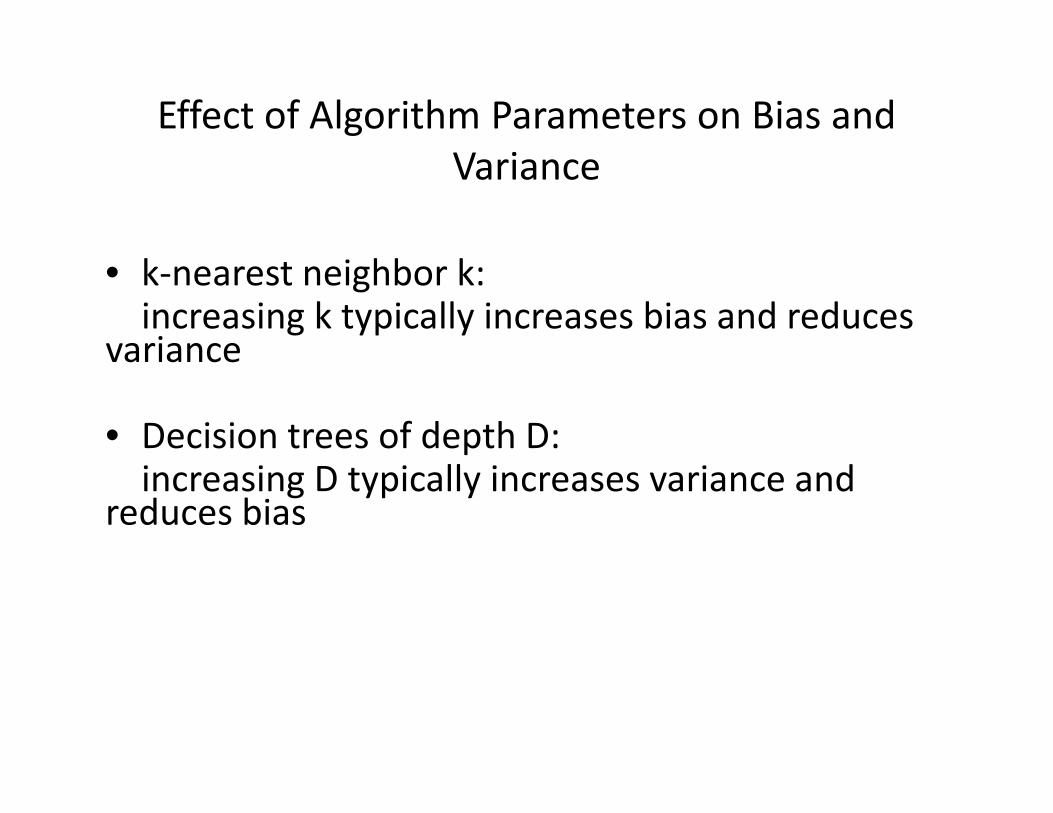
Effect of Algorithm Parameters on Bias and Variance

• k‐nearest neighbor k:  increasing k typically increases bias and reduces 

variance

• Decision trees of depth D: increasing D typically increases variance and 

reduces bias

Why does bagging work?

• Bagging takes the average of multiple models ‐‐‐ reduces the variance

• This suggests that bagging works the best with low bias and high variance classifiers such as …

• Un‐pruned decision trees• Bagging typically will not hurt the performace

Boosting

Boosting

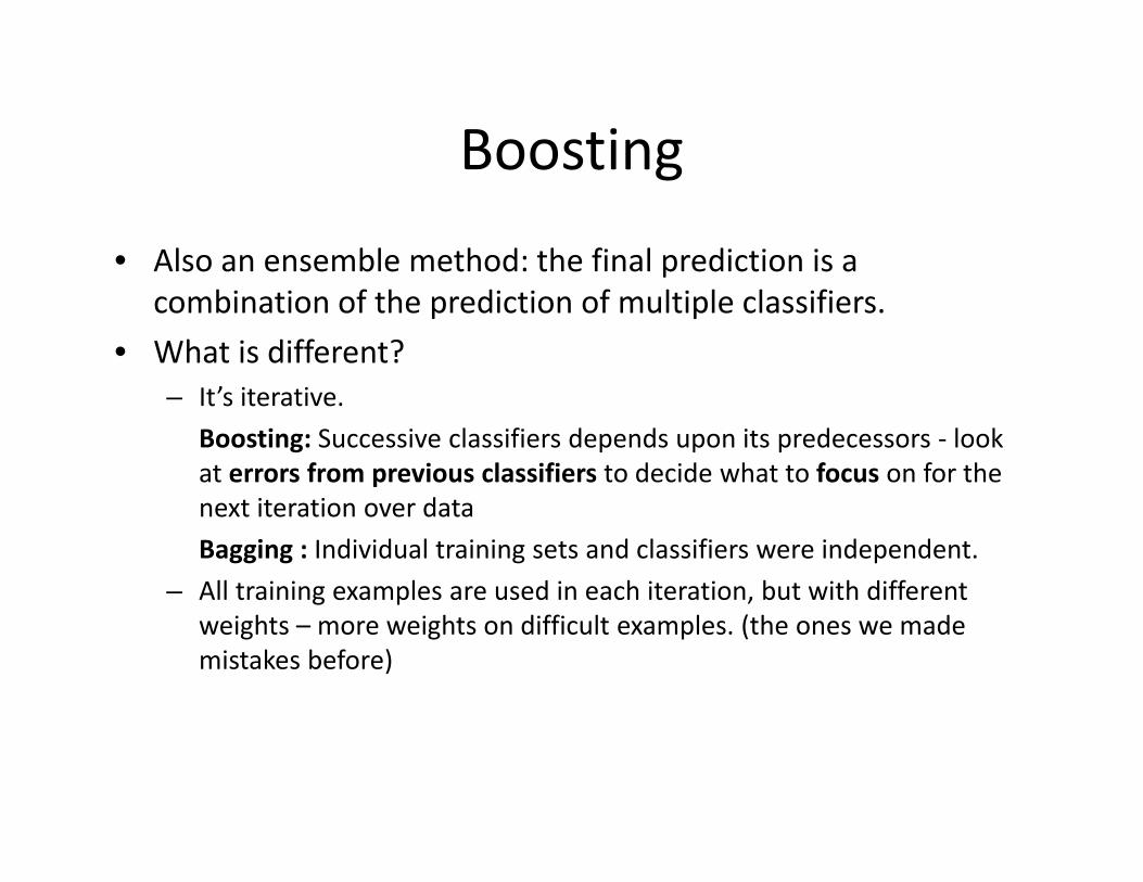
• Also an ensemble method: the final prediction is a combination of the prediction of multiple classifiers.

• What is different?– It’s iterative. 

Boosting: Successive classifiers depends upon its predecessors ‐ look at errors from previous classifiers to decide what to focus on for the next iteration over dataBagging : Individual training sets and classifiers were independent.

– All training examples are used in each iteration, but with different weights – more weights on difficult examples. (the ones we made mistakes before)

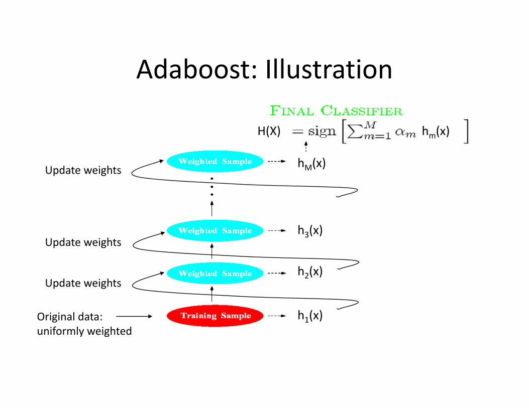
Adaboost: Illustration

Original data: uniformly weighted

Update weights

Update weights

Update weights

h1(x)

h2(x)

h3(x)

hM(x)

hm(x)H(X)

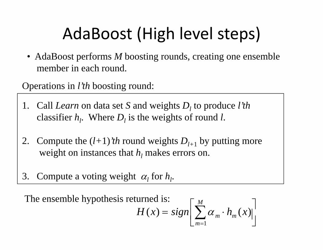
AdaBoost (High level steps)

1. Call Learn on data set S and weights Dl to produce l’thclassifier hl. Where Dl is the weights of round l.

2. Compute the (l+1)’th round weights Dl+1 by putting more weight on instances that hl makes errors on.

3. Compute a voting weight l for hl.

• AdaBoost performs M boosting rounds, creating one ensemble member in each round.

Operations in l’th boosting round:

The ensemble hypothesis returned is:

M

mmm xhsignxH

1)()(

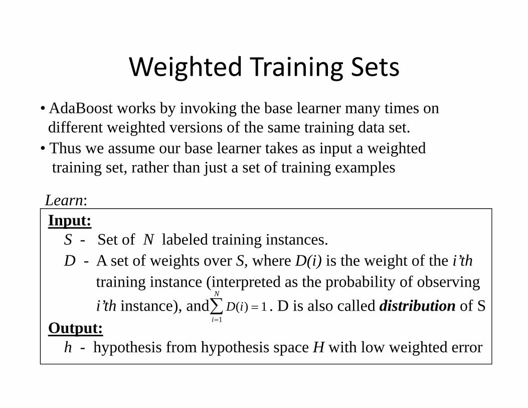
Weighted Training Sets• AdaBoost works by invoking the base learner many times on different weighted versions of the same training data set.

• Thus we assume our base learner takes as input a weightedtraining set, rather than just a set of training examples

Learn:Input:

S - Set of N labeled training instances.D - A set of weights over S, where D(i) is the weight of the i’th

training instance (interpreted as the probability of observingi’th instance), and . D is also called distribution of S

Output:h - hypothesis from hypothesis space H with low weighted error

D ii

N

( ) 1

1

Definition: Weighted Error

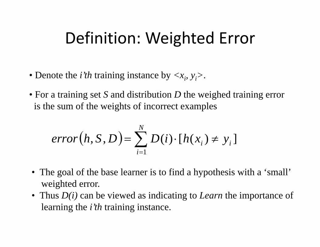
• Denote the i’th training instance by <xi, yi>.

• For a training set S and distribution D the weighed training erroris the sum of the weights of incorrect examples

N

iii yxhiDDSherror

1

])([)(,,

• The goal of the base learner is to find a hypothesis with a ‘small’weighted error.

• Thus D(i) can be viewed as indicating to Learn the importance of learning the i’th training instance.

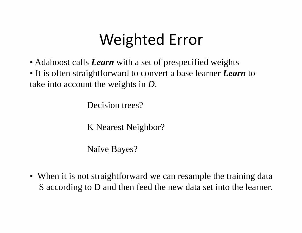
Weighted Error• Adaboost calls Learn with a set of prespecified weights • It is often straightforward to convert a base learner Learn to take into account the weights in D.

Decision trees?

K Nearest Neighbor?

Naïve Bayes?

• When it is not straightforward we can resample the training dataS according to D and then feed the new data set into the learner.

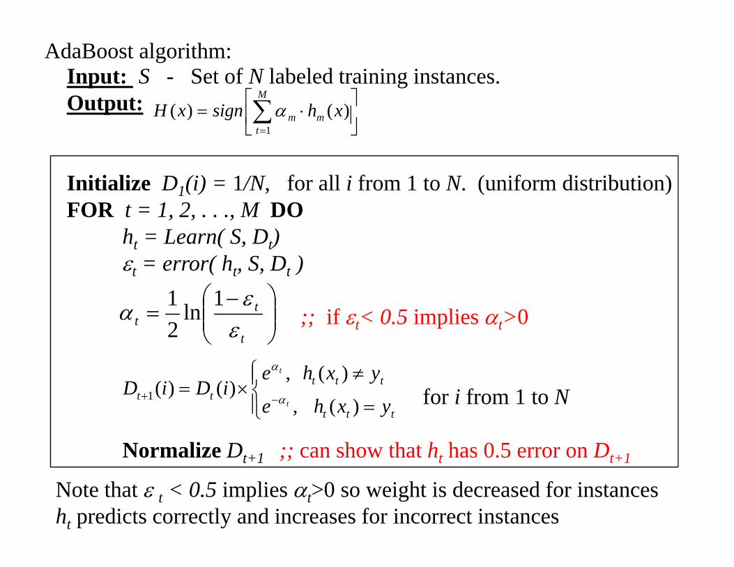
AdaBoost algorithm:Input: S - Set of N labeled training instances.Output:

Initialize D1(i) = 1/N, for all i from 1 to N. (uniform distribution)FOR t = 1, 2, . . ., M DO

ht = Learn( S, Dt)t = error( ht, S, Dt )

;; if t< 0.5 implies t>0

for i from 1 to N

Normalize Dt+1 ;; can show that ht has 0.5 error on Dt+1

ttt

ttttt

yxhe

yxheiDiD

t

t

)(,

)(,)()(1

t

tt

1ln21

Note that t < 0.5 implies t>0 so weight is decreased for instancesht predicts correctly and increases for incorrect instances

M

tmm xhsignxH

1

)()(

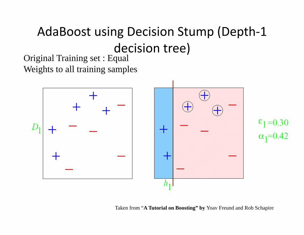
AdaBoost using Decision Stump (Depth‐1 decision tree)

Original Training set : Equal Weights to all training samples

Taken from “A Tutorial on Boosting” by Yoav Freund and Rob Schapire

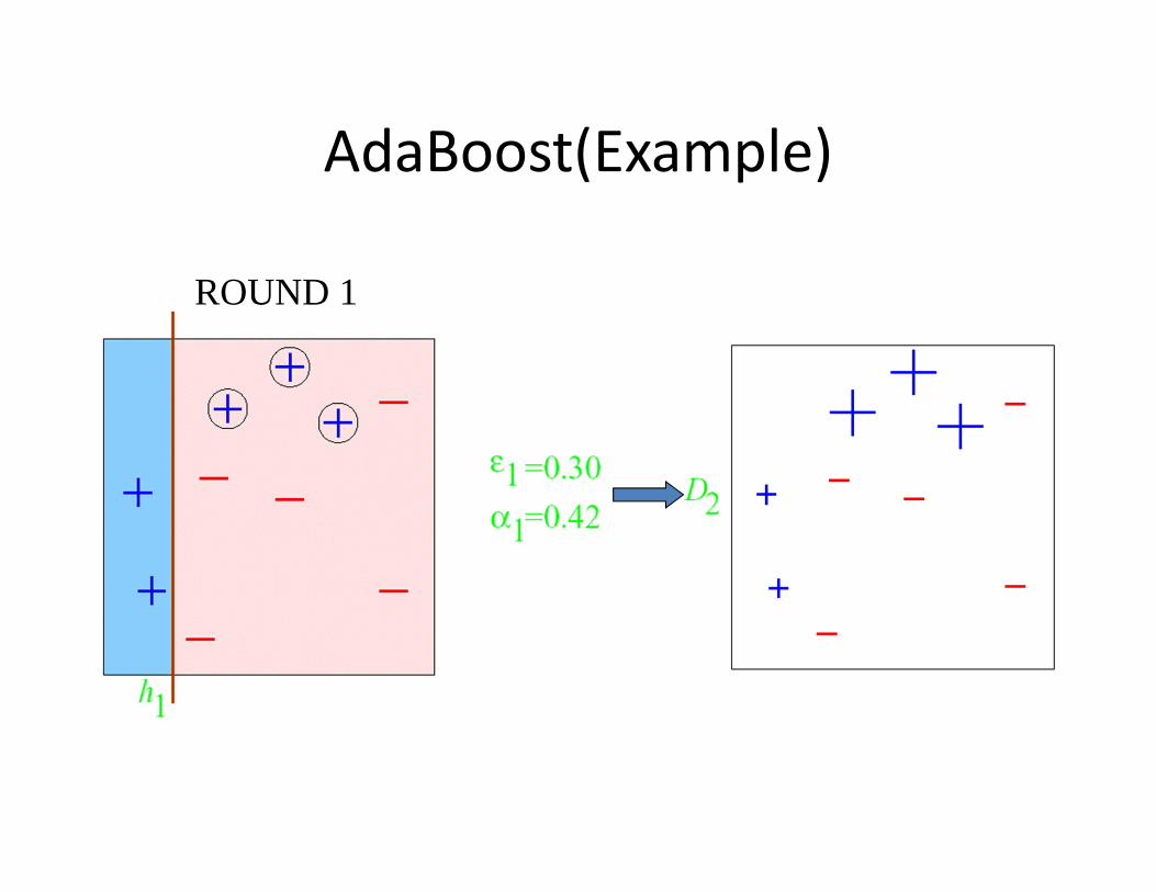
AdaBoost(Example)

ROUND 1

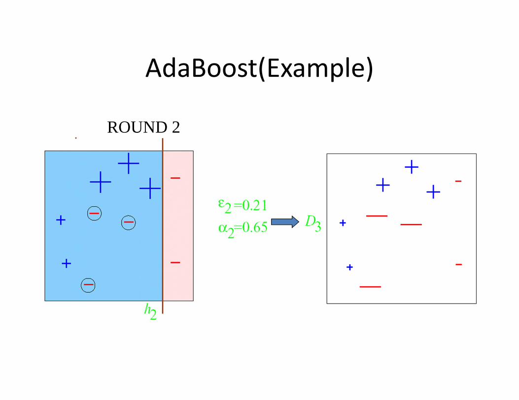
AdaBoost(Example)

ROUND 2

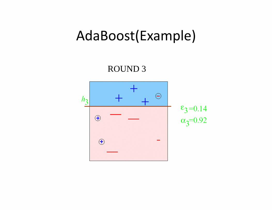
AdaBoost(Example)

ROUND 3

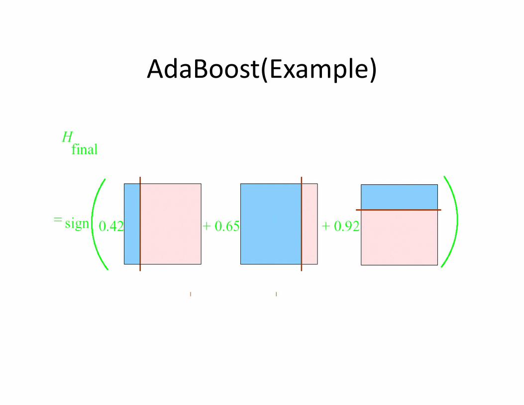
AdaBoost(Example)

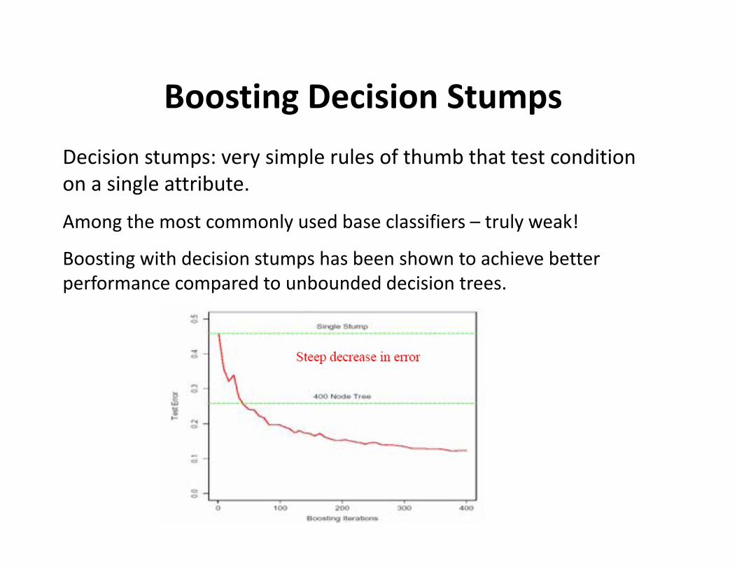
Boosting Decision StumpsDecision stumps: very simple rules of thumb that test condition on a single attribute.

Among the most commonly used base classifiers – truly weak!

Boosting with decision stumps has been shown to achieve better performance compared to unbounded decision trees.

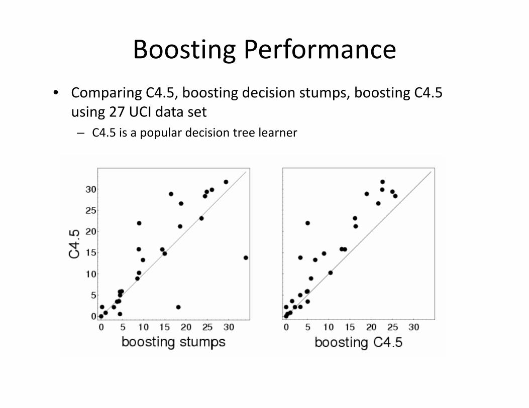
Boosting Performance• Comparing C4.5, boosting decision stumps, boosting C4.5 

using 27 UCI data set– C4.5 is a popular decision tree learner

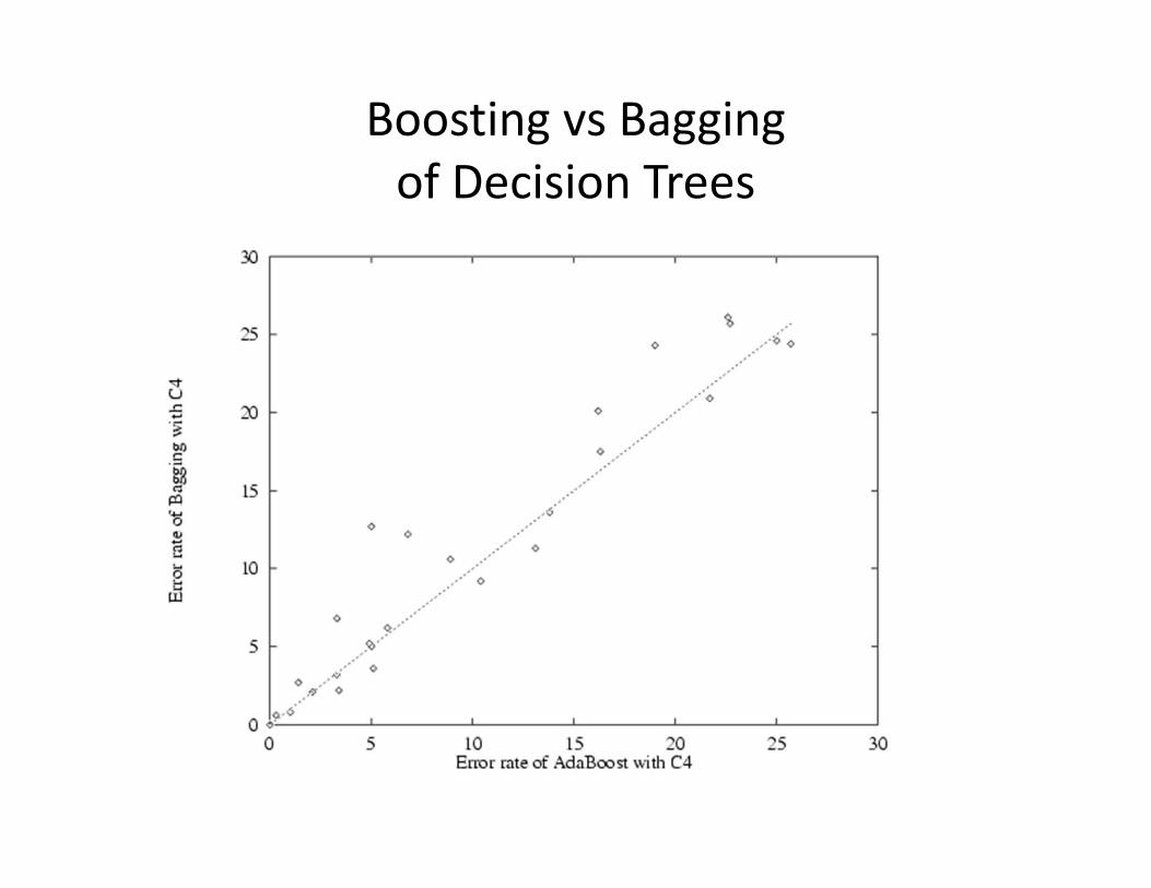
Boosting vs Baggingof Decision Trees

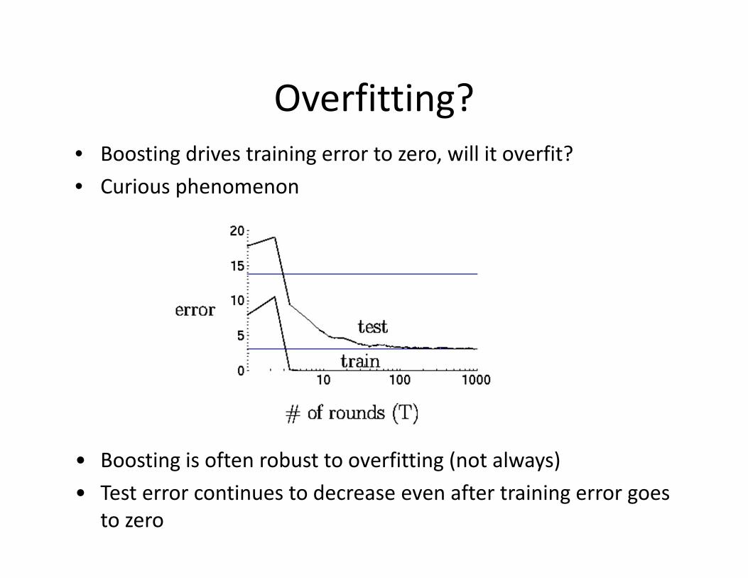
Overfitting?• Boosting drives training error to zero, will it overfit?• Curious phenomenon

• Boosting is often robust to overfitting (not always)• Test error continues to decrease even after training error goes 

to zero

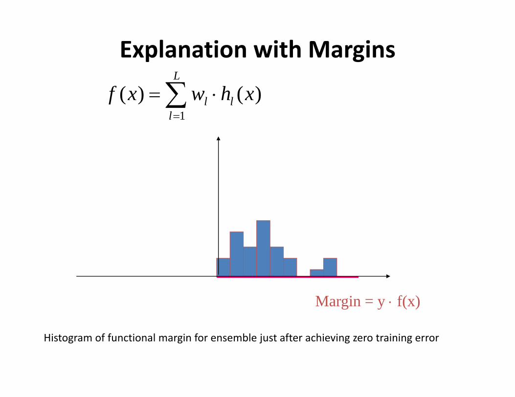
Explanation with Margins

Margin = y f(x)

Histogram of functional margin for ensemble just after achieving zero training error

L

lll xhwxf

1)()(

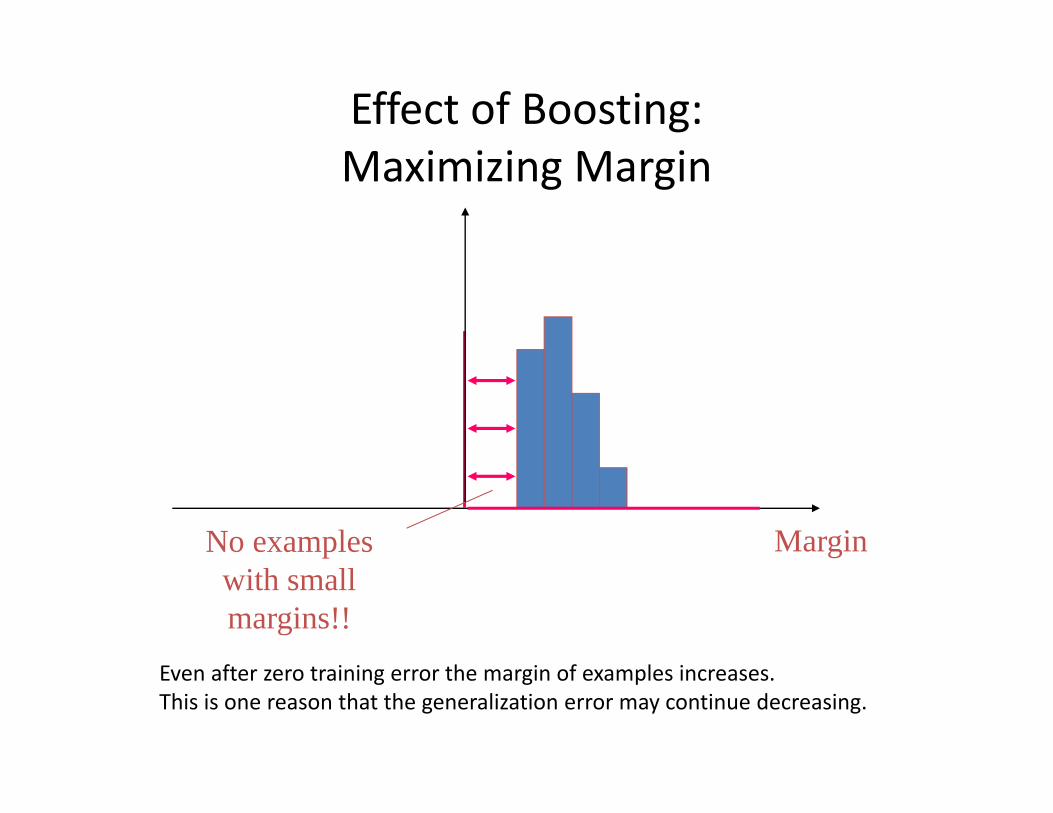
Effect of Boosting: Maximizing Margin

MarginNo examples with small margins!!

Even after zero training error the margin of examples increases.This is one reason that the generalization error may continue decreasing.

Bias/variance analysis of Boosting

• In the early iterations, boosting is primary a bias‐reducing method

• In later iterations, it appears to be primarily a variance‐reducing method

What you need to know about ensemble methods?

• Bagging: a randomized algorithm based on bootstrapping– What is bootstrapping– Variance reduction– What learning algorithms will be good for bagging?  ‐ high variance, 

low bias ones such as unpruned decision trees

• Boosting:– Combine weak classifiers (i.e., slightly better than random)– Training using the same data set but different weights– How to update weights?– How to incorporate weights in learning (DT, KNN, Naïve Bayes)– One explanation for not overfitting: maximizing the margin