ensemble simulations of explosive cyclogenesis at ranges...

2920 VOLUME 128M O N T H L Y W E A T H E R R E V I E W

q 2000 American Meteorological Society

Ensemble Simulations of Explosive Cyclogenesis at Ranges of 2–5 Days

FREDERICK SANDERS

Marblehead, Massachusetts

STEVEN L. MULLEN

Institute of Atmospheric Physics, The University of Arizona, Tucson, Arizona

DAVID P. BAUMHEFNER

National Center for Atmospheric Research, Boulder, Colorado

(Manuscript received 29 March 1999, in final form 1 February 2000)

ABSTRACT

Ensemble simulations of explosive cyclogenesis are examined in a lengthy run of a global general circulationmodel with the perfect ensemble context. Attention is focused on the day when the deepest low appeared. Anensemble of 31 members is obtained by integrating 30 additional runs starting from slightly perturbed initialconditions. The perturbations are randomly selected to represent equal approximations to the truth, given typicalanalysis differences between major centers. Ensembles are generated starting two, three, four, and five days priorto maximum depth. Two lows are contrasted, the deepest low near Kamchatka and a marginally explosive lowover the central Pacific.

The early development of both systems was suppressed by their presence in the confluent entrance region ofthe Pacific winter jet. An intense low near Kamchatka eventually developed in each member of the ensembleat all projections, but the details of development varied from member to member and were related to theinvolvement of a surface perturbation coming up into the system from low latitudes. In contrast, cyclogenesisover the central Pacific occurred in some members of the ensemble but not at all in others. The difference inbehavior of the two systems is reflected in a localized enhancement of the error growth of the planetary andsynoptic scales for the central Pacific low and is related to the smaller horizontal scale of the central Pacificlow.

Probabilistic estimates of precipitation quantity and surface wind speeds produced by the ensemble showedmoderate skill at day 5 with respect to climatology, mainly away from the regions of most vigorous synopticactivity, when verified against individual ensemble members. Skill would be reduced if the ensemble meanproved to be more seriously in error as is the case for a forecast verified against observations.

1. Introduction

The sudden development of intense cyclones over theoceans of mid- and high latitudes during the cold season(Sanders and Gyakum 1980) is an important forecastingchallenge, because these systems typically producewinds of gale or storm force in 24 hours or less. It hasbeen suggested that the predictability of these storms atranges of 1–2 days may be less than that of other lessintense cyclones (Kallen and Huang 1988; Mullen andBaumhefner 1988, 1989; Kuo and Low-Nam 1990).Hence, it is desirable to evaluate the degree to whichrapidly intensifying storms are sensitive to uncertainlyof initial conditions at longer ranges and determine

Corresponding author address: Dr. Frederick Sanders, 9 FlintStreet, Marblehead, MA 01945.E-mail: [email protected]

whether the predictability of particular baroclinic struc-tures can be different.

We have undertaken to do this by utilizing a longintegration of the Community Climate Model Version2 (CCM2) produced at the National Center for Atmo-spheric Research (NCAR). This model has been de-scribed by Hack et al. (1993) and was run at a spectralresolution of triangular 63 (T63). This resolution is vir-tually the same as that for the operational medium-rangeensemble prediction system at the National Centers forEnvironmental Prediction (Tracton and Kalnay 1993).We studied a 180-day simulation initialized with theanalysis of observations at 0000 UTC 1 October 1975.Although the resemblance of the simulation to the realatmosphere as represented by observations is surely lim-ited to a few days (e.g., Lorenz 1982), the model appearsto produce realistic-looking patterns indefinitely. Fur-thermore, Sanders and Mullen (1996) showed that the

AUGUST 2000 2921S A N D E R S E T A L .

FIG. 1. Sea level isobars at intervals of 4 mb on day 102.5 for theunperturbed run starting at day 97.5. Longitude lines are at intervalsof 108, from 908W to 1108E. Latitude lines are at intervals of 108,from 208 to 708N.

FIG. 3. Same as Fig. 1, but for day 101.5.

FIG. 4. Same as Fig. 2, but for day 101.5.

FIG. 2. 500-mb height contours at intervals of 6 dam for day 102.5for the unperturbed run starting at day 97.5. The 534 and 552 damcontours are thickened. Latitude and longitude as in Fig. 1.

climatology of explosive cyclogenesis in this model wassimilar to that in the real atmosphere with respect tofrequency, intensity, and location, suggesting that theT63 CCM2 can be used with confidence for predict-ability experiments.

2. Selection of case

We chose to study simulations of two to five days’duration, all verifying at day 102.5 (corresponding to acalendar date of 1200 UTC 10 January 1976) of the180-day run. This time was the end of the largest 24-hdeepening in the run, in a cyclone with a central pressureof 934 mb that lay along the east coast of the Kamchatkapeninsula (Fig. 1). It was accompanied by a deep lowat 500 mb (Fig. 2) almost directly overhead, flanked onits east and south sides by a strong jet.

Twenty-four hours earlier, the 985-mb cyclone wasnear 408N latitude and 1408E longitude (Fig. 3). Aslightly deeper low lay over the Sea of Okhotsk, justwest of Kamchatka, but it lost its identity as the stronglydeepening center moved up from the south-southwest.

At 500 mb (Fig. 4) a pronounced trough lay just westof the surface center, so the explosive deepening oc-curred in a scenario similar to that described by Sanders(1986).

A second cyclone, in the central Pacific at lower lat-itudes (Figs. 1 and 2) deepened just enough to qualifyas a ‘‘bomb’’ according to the criterion of Sanders andGyakum (1980). It was also accompanied by a pro-nounced 500-mb trough just upstream from the surfacecenter. Additional deep cyclones lay in the Gulf of Alas-ka and over the central United States at the edge themap on day 102.5 (Fig. 1). The first of these deepenedexplosively over the western Pacific between days 97.5and 98.5, while the other qualified as a bomb off thecoast of Oregon in the 24-h period ending on day 101.5(Fig. 3). These cyclones were not studied.

3. The ensembles

Four ensembles, each with 30 members, were pro-duced by running the identical model from slightly per-turbed initial conditions. The four ensembles were ini-tiated on days 97.5, 98.5, 99.5, and 100.5, representingranges from two to five days before the verifying day102.5. The perturbations were obtained by the simula-tion of analysis differences, as described by Errico andBaumhefner (1987), Mullen and Baumhefner (1989),


FIG. 5. Difference in initial 500-mb height (meters), ensemblemembers 14 minus 21 for initial time (IT) 97.5. Isopleths are every65 m, 615 m, 625 m, . . . , with magnitudes above 15 m stippled.

FIG. 6. Contours of initial ensemble-mean 500-mb height (solid),at intervals of 6 dam, for IT 97.5. Dashed lines are isopleths of rmsvalue of 500-mb height perturbation after initialization, at intervalsof 1 dam. Light stippling indicates values greater than 1 dam; heavystippling indicates values greater than 2 dam.

and Du et al. (1997), and were designed to representequally likely representations of the truth given typicalanalysis errors. An example of such perturbations, afterinitialization (Errico 1983), appears in Fig. 5 for the500-mb height field at day 97.5, while the standard de-viation for the perturbations about the ensemble meanappears in Fig. 6. The figures indicate that perturbationstend to be largest over the midlatitude storm tracks andnear small-scale features such as short-wave troughs,and smallest over the continents and low latitudes, inaccord with estimates of analysis uncertainty (Daley andMayer 1986; Augustine et al. 1991; see Fig. 3a of Nutteret al. 1998).

4. Definition of verification and error

In presentation of results, it is necessary to measureerror in the context of this long model run. In an op-erational environment, error is usually obtained by com-paring the forecast against an observation or an analysisbased on observations. Since this is not possible in thepresent case, as noted above, something from the modelrun itself must be used as verification. The two possi-bilities are the unperturbed run, which was used for theselection of the case, and an ensemble of analyses withinitialized perturbations added to the unperturbed runfor all verification times. Since by design the globalaverage of the initial perturbations is zero (Mullen andBaumhefner 1989), these two measures will be approx-imately the same at the initial time. Moreover, sinceverification is needed for times at which no initializedperturbations were generated (i.e., days 98.0, 99.0,100.0, and 101.0–102.5) and for fields (i.e., precipi-tation) that are not initially perturbed, the unperturbedrun seems the most appropriate choice in this circum-stance.

On the other hand, since the result of the unperturbedrun would have been different had the initial conditionsbeen perturbed and subsequently evolved by the modelas described above, the unperturbed run has no claim

to special consideration. Therefore, the error for all ver-ification times is determined by cross validation (Wilks1995, pp. 194–198), whereby each ensemble memberin turn is taken as verification and compared against allremaining ensemble members, started from the sameinitial time. The results of these comparisons are thenaveraged and are considered as the error of the simu-lation.

The experimental design is patterned after the ‘‘per-fect ensemble’’ system described by Buizza (1997),where one member is randomly selected to serve asverification for the remaining members. The perfect en-semble assumption maximizes skill, since model erroris not considered and a perfect knowledge of analysiserror statistics is assumed. When interpreting the resultsof this paper, the reader should kept in mind that ourexperiment yields an estimate of an upper bound onensemble accuracy.

5. The ensemble simulations

a. Simulations for the Kamchatka cyclone

Histograms of central pressure for the Kamchatka cy-clone in the 31 runs (the single unperturbed and 30perturbed cases) appear in Fig. 7. A deep center wasfound in every run, ranging from 960 to 920 mb (to thenearest 5 mb) at a 5-day range, shrinking to a smallestrange, from 955 to 930 mb at a 2-day range. The dif-ference between extreme members oscillated with initialtime, however, with a range (to the nearest 5 mb) of 40,30, 40, and 25 mb at day 5 through day 2, respectively.The means and medians of central pressure exhibitedsimilar behavior, gradually shifting toward weaker sys-tems from day 5 to day 3 range (medians of 936, 944,and 952 mb, respectively), away from the unperturbedvalue of 934 mb, then abruptly jumping toward muchdeeper values at day 2 range (median of 939 mb). It isunclear whether this behavior has an underlying dy-


FIG. 7. Histograms of central pressure for the Kamchatka low atsea level to nearest 5 mb, for all 31 ensemble members at valid time(VT) 102.5. IT indicated in upper right side of each panel. The centralpressure for the unperturbed cyclone is 934 mb.

FIG. 9. Sea level isobars at intervals of 4 mb for member 23 start-ing at IT 97.5 valid at VT 101.5.

FIG. 10. Same as Fig. 9, but for member 13.

FIG. 8. Ensemble-mean sea level isobars at intervals of 4 mb, forIT 97.5, VT102.5. Stippling denotes regions where the ensemble var-iance exceeds the model’s climatological variance. Latitude and lon-gitude lines as in Fig. 1.

namical cause, such as some earlier lead times beingmore sensitive to initial error than later ones, or rep-resents a sampling fluctuation (ensemble size too small).The distributions at day 2 are consistent with the earlierresults of Mullen and Baumhefner (1994) at coarserresolution. In the few weaker ensemble members at

ranges of 3 and 4 days, the one-bergeron criterion ofSanders and Gyakum (1980) was not met during the24-h period ending at day 102.5, but a significant lowwas nevertheless found. The ensemble-mean sea levelpressure pattern at day 102.5, in the ensemble initiatedfive days earlier, appears as Fig. 8. The center is slightlynorthwest of the position in the unperturbed run, andthe central pressure of 948 mb is less deep than the 936-mb median value. The reason for the discrepancy inposition is that ensemble members with lower pressureslay northwest of the others. The difference in centralpressure is due to variability of position of the centerin the ensemble members.

There was also some variability within the ensemblein the mode of development of the system. In about halfthe members a low formed in an inverted trough nearTaiwan at the beginning of the run and became a deep-ening system. Ensemble member 23 shows an exampleof this behavior. The low just east of Japan on day 101.5(Fig. 9) initiated as a weak center at the northern tip ofTaiwan 36 h earlier and ended with a central pressureof 920 mb west of Kamchatka 24 h later. In other in-stances, the low west of Kamchatka was the deeperthroughout. An example is seen in Fig. 10, which pro-duced the weakest low in the ensemble. The low overthe Sea of Okhotsk remained the deepest on the map,


FIG. 11. Histograms of distances of center of Kamchatka low atsea level from position of ensemble mean low, in degrees of latitude(110 km), for all 31 ensemble at VT 102.5. IT is indicated in upperright side of each panel.

FIG. 12. Ensemble-mean sea level isobars at intervals of 4 mb, forIT 98.5 VT 102.5. Stippling denotes regions where the ensemblevariance exceeds the climatological variance. Latitude and longitudelines as in Fig. 1.

while the weak center over Taiwan never intensifiedsignificantly in this run. The model atmosphere, so tospeak, knew where it wanted to go but was uncertainof the route taken to reach the goal. In those 16 membersof the ensemble showing the deepest low south of 508Nlatitude at some point in the run, the average final centralpressure was about 933 mb, while in the 15 others theaverage was about 942 mb.

The variability of position of the final deep low withinthe ensembles is illustrated by the histograms in Fig.11. The median distance of the centers in the individualensemble members from the position of the ensemble-mean low shrank from about 58 latitude (550 km) at arange of 5 days to less than 220 km at 2-day range.Median distances at ranges of 5 and 3 days were vir-tually the same, presumably because of the influence ofthe low from Taiwan. The greatest difference in positionfor an ensemble member was about 1000 km in the runinitiated at day 97.5.

b. Simulations for the central Pacific cyclone

The cyclone over the central Pacific displayed a dif-ferent ensemble behavior. Although the unperturbed runshowed a distinct and substantial center on day 102.5

(Fig. 1), the ensemble mean for this time initiated atday 97.5 showed a barely identifiable center in the re-gion of col between two substantial anticyclones (Fig.8). In the run initiated 24 h later (Fig. 12), there was adistinct center, albeit one still substantially less intensethan that in the unperturbed run. This behavior appearsto be an example in the ensemble mean fields of a ‘‘fore-cast fracture’’ (Sanders 1992), an abrupt difference inmodel solutions from consecutive runs valid at the sametime. The comparison between the unperturbed run andthe ensemble mean implies considerable variabilityamong the ensemble members. Enhanced variability isalso indicated in Figs. 8 and 12 by the stippling ofregions where the standard deviation about the ensembleexceeds the climatic variance for the CCM2.

This variability is further confirmed by the histogramsin Figs. 13 and 14. So far as central pressure is con-cerned, Fig. 13 shows a broad range of values. At 5-dayrange, two ensemble members had a central pressurenear 1020 mb, as in the ensemble mean. The unper-turbed run yielding 996 mb (Fig. 1) was one of thedeeper members, although two others reached about 980mb. The substantial number of ‘‘no-low’’ members atthis 5-day range were determined subjectively on thebasis of the absence of a low (no ‘‘L’’ symbol on a map)of significant depth within 1500 km of the position ofthe ensemble-mean low. The variability of positions andcentral pressures among the ensemble members shrankat the shorter ranges but remained substantially greaterthan the variability for the Kamchatka cyclone for allinitial times. The difference in variability between thetwo cases is greatly enhanced when a comparison ismade between the unperturbed or ensemble-mean valuesof the lows and the climatological mean values. Thecentral pressure for the Kamchatka low is far below theclimatological mean, while that for the central Pacificlow is relatively close to it.

As examples of extremes of this variability in the runsinitiated at day 97.5, we show maps of sea level pressureand 500-mb height for ensemble members 14 (Figs. 15


FIG. 13. Histograms of central pressure for the central Pacific lowat sea level, to nearest 5 mb, for all 31 ensemble members at VT102.5. IT is indicated in upper right side of each panel. NL meansno low was present (see text). The central pressure for the unperturbedcyclone is 996 mb.

FIG. 14. Histograms of distance of the central Pacific low at sealevel from position of ensemble mean low, in degrees of latitude (110km), for all 31 ensemble members at VT 102.5. NL means no lowwas present. IT is shown in upper right side of each panel.

FIG. 15. Sea level isobars at intervals of 4 mb for ensemblemember 14, IT 97.5 VT 102.5. Latitude and longitude lines as inFig. 1.

and 16) and 21 (Figs. 17 and 18). In the former pairthere is a sea level cyclone over the central Pacific re-sembling that seen in the unperturbed run (Fig. 1) butconsiderably deeper. Aloft there is a pronounced troughwith a weak low center, roughly coincident with thesurface system. In contrast, member 21 displays at sealevel a 1043-mb high slightly west of the low in Fig.15, and no low at all within about 3000 km. At 500 mb,we see a less pronounced trough east of the surface high.Note that the position and central pressure of the lownear Kamchatka varies relatively little (550 km and 10mb, respectively) in these two ensemble members.

6. Difference in predictability

The difference in ensemble behavior between the twocyclones seems to imply something about smaller pre-dictability for the Pacific storm.

If we can reliably assert that the probability of someevent (of whatever character involving whatever weath-er element) is different from some ‘‘control’’ probabil-ity, then we can say we have some predictability of thatevent. The no-skill control in this case could be eitherpersistence of the current condition or ‘‘climatology’’

(the average condition suitably defined) or some simplecombination of the two, such as persistence expectancy.

Let us now consider predictability of the sea levelpressure field in our simulations. We say that the dis-persion of the ensemble about its mean value is to becompared with the ‘‘climatological variance’’ at thesame location, by which we mean the dispersion of daily


FIG. 16. Contours of 500-mb height, at intervals of 6 dam, for en-semble member 14, IT 97.5 VT 102.5.

FIG. 17. Same as Fig. 16, but for ensemble member 21.

FIG. 18. Same as Fig. 17, but for ensemble member 21.

(or other) values about the mean during all or some partof the simulation run. If the variance of the ensembleis larger than the climatological variance at that location,we might say that there is no predictability in the sensethat the average difference between two ensemble mem-bers exceeds the average difference between days se-lected at random from the climatological distribution.But this assertion neglects the fact that the verificationmay be far from the climatological mean value, as forexample in the vicinity of the Kamchatka low, as op-posed to the vicinity of the Pacific low, where verifi-cation is relatively close to the climatological mean.Hence, the probability distribution for the ensemble nearKamchatka (where the probability of a value below, say,950 mb is much greater then its climatological value)may be quite different from the climatological distri-bution. Then the skill of the ensemble may be positivewith respect to the climatological competitor, althoughthe ensemble variance is larger than the climatologicalvariance.

Some insight into the difference in behavior of thesetwo systems in the ensemble can be obtained from Fig.6. Over the western Pacific Ocean and eastern Asia onday 97.5, there were two major troughs at 500 mb. Oneof these was oriented nearly east–west over Siberia justnorth of latitude 608N, while the other was orientednearly meridionally just east of the Japanese islands.These were associated respectively with the develop-ment of the Kamchatka cyclone and the low in the Gulfof Alaska (not studied). The development of the lowover the central Pacific was related to the weak troughin the northwesterly flow near 458N, 1008E, just down-wind of the Kamchatka trough. Figure 6 shows that theroof-mean-square (rms) value of the height perturba-tions over the Pacific was substantially greater thanthose over the Asian continent, reflecting the greateranalysis uncertainty over the oceanic region of sparsedata.

Since both troughs lay over the continental region ofsmall uncertainty at day 97.5, however, a difference inthe size of the initial perturbations is not a likely factor.

In fact, differences between the initial 500-mb analysesat day 97.5 for extreme members 14 and 21 (Fig. 5)were small. A similar sensitivity to small initial differ-ences, as reflected in analyses from different operationalcenters, was obtained by Rabier et al. (1996, their Figs.3 and 4) for a case of cyclogenesis over the North At-lantic. Rabier et al. (1996) show through linear adjointanalysis how small initial perturbations in dynamicallysensitive regions can lead to widely divergent outcomes.In light of the analysis of Rabier et al., it is possiblethat our initial perturbations, which are not dynamicallyconditioned, project on such dynamically sensitivestructures that were not quantified in this study.

On the other hand, the horizontal scales of the initial500-mb troughs associated with the two systems, andwith the subsequent upper-level troughs and surfacelows, were quite different, substantially larger for theKamchatka low. This initial 500-mb trough was muchmore pronounced than the trough associated with thecentral Pacific low. The large difference of outcome isalso believed to be related, in part, to the different scalesof the systems, reflecting their prominence as synopticfeatures.

As a measure of the difference in character of thetwo troughs, the initial maximum point geostrophic vor-ticity was obtained for each trough for each member of


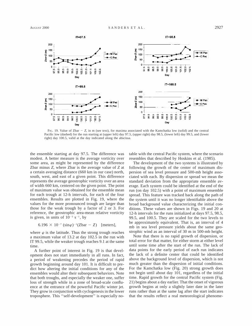
FIG. 19. Value of Zbar 2 Z, in m (see text), for maxima associated with the Kamchatka low (solid) and the centralPacific low (dashed) for the run starting at (upper left) day 97.5, (upper right) day 98.5, (lower left) day 99.5, and (lowerright) day 100.5, valid at the day indicated along the abscissa.

the ensemble starting at day 97.5. The difference wasmodest. A better measure is the average vorticity oversome area, as might be represented by the differenceZbar minus Z, where Zbar is the average value of Z ata certain averaging distance (660 km in our case) north,south, west, and east of a given point. This differencerepresents the average geostrophic vorticity over an areaof width 660 km, centered on the given point. The pointof maximum value was obtained for the ensemble meanfor each trough at 12-h intervals, for each of the fourensembles. Results are plotted in Fig. 19, where thevalues for the more pronounced trough are larger thanthose for the weak trough by a factor of 2 or 3. Forreference, the geostrophic area-mean relative vorticityis given, in units of 1025 s21, by

6.196 3 1027 (sinw)21(Zbar 2 Z) [meters],

where w is the latitude. Thus the strong trough reachesa maximum value of 13.2 at day 102.5 in the run withIT 99.5, while the weaker trough reaches 9.1 at the sametime.

A further point of interest in Fig. 19 is that devel-opment does not start immediately in all runs. In fact,a period of weakening precedes the period of rapidgrowth beginning around day 101. It is difficult to pre-dict how altering the initial conditions for any of theensembles would alter their subsequent behaviors. Notethat both troughs, and especially the weaker one, sufferloss of strength while in a zone of broad-scale conflu-ence at the entrance of the powerful Pacific winter jet.They grow in conjunction with cyclogenesis in the lowertroposphere. This ‘‘self-development’’ is especially no-

table with the central Pacific system, where the scenarioresembles that described by Hoskins et al. (1985).

The development of the two systems is illustrated byfollowing the growth of the center of maximum dis-persion of sea level pressure and 500-mb height asso-ciated with each. By dispersion or spread we mean thestandard deviation from the appropriate ensemble av-erage. Each system could be identified at the end of therun (on day 102.5) with a point of maximum ensemblespread. This feature was tracked back along the path ofthe system until it was no longer identifiable above thebroad background value characterizing the initial con-ditions. These values are shown in Figs. 19 and 20 at12-h intervals for the runs initialized at days 97.5, 98.5,99.5, and 100.5. They are scaled for the two levels tobe approximately equivalent. That is, an interval of 4mb in sea level pressure yields about the same geo-strophic wind as an interval of 30 m in 500-mb height.

Note that there is no rapid growth of dispersion, ortotal error for that matter, for either storm at either leveluntil some time after the start of the run. The lack ofdata points for the early period of each run indicatesthe lack of a definite center that could be identifiedabove the background level of dispersion, which is notmuch greater than the dispersion of initial conditions.For the Kamchatka low (Fig. 20) strong growth doesnot begin until about day 101, regardless of the initialtime. Rapid growth for the central Pacific system (Fig.21) begins about a day earlier. That the onset of vigorousgrowth begins at only a slightly later date in the laterruns rather than at the same lag after the start indicatesthat the results reflect a real meteorological phenome-


FIG. 20. Ensemble spread for the maximum associated with the Kamchatka low, for sea level pressure (in mb, solid)and for 500-mb height (in m, dashed) for the run starting at (upper left) day 97.5, (upper right) day 98.5, (lower left)day 99.5, and (lower right) day 100.5, and valid at the times shown along the abscissa.

non, likely related to the dynamic sensitivity of flowinstabilities to initial perturbations. The dispersion byday 102.5, however, is not as large for the runs initiatedlater than for the earlier runs, and error growth continuesto the end of each run, suggesting that further growthmight have occurred had the later runs been carriedfarther. Once significant growth of dispersion begins,its doubling time is usually between half a day and oneday, slightly less for the central Pacific storm. The rea-son for this difference in behavior is not known. Themaximum dispersions reached for the central Pacific loware slightly larger than those for the Kamchatka system,despite its lesser strength in the ensemble mean, indi-cating less predictability for the former cyclone.

Further implications of reduced predictability are seenif these dispersions are compared with the deviation ofthe ensemble mean from the climatological mean. Thevalues for the Pacific case are much larger, since theensemble mean is relatively close to the climatologicalmean. Hence, the central Pacific development can beregarded as less predictable, as also indicated by theerratic occurrence of explosive deepening among theensemble members.

Examination of the flow indicated by the Zbar fieldsshows that both vorticity maxima on day 97.5, partic-ularly that for the central Pacific low, lay in the entranceregion of a large-scale jet over the central Pacific (Fig.22). The latter, already elongated along the flow, isstretched even farther because of conservation of vor-ticity in the confluent flow containing considerable de-formation. Farrell (1989) has shown that a disturbance,elongated normal to the flow, would amplify in termsof disturbance energy and central deficit of stream-

function (or height) in such a confluent flow. His anal-ysis, if applied to our situation of along-flow elongationin confluence, would no doubt indicate weakening ofthe disturbance, as we have seen. This confluence ispresent in all members of the ensemble but weakens asthe disturbance travels eastward, vanishing around day100, shortly before the onset of development in the un-perturbed run as well as in those ensemble membersyielding the most and least cyclogenesis over the centralPacific. We infer than the confluence inhibits develop-ment that might otherwise have occurred.

7. Types A and B cyclogenesis

This situation calls to mind the distinction drawn byPetterssen and Smebye (1971) between type A and typeB cyclogenesis. They assert, inter alia, that in type A‘‘development occurs under a more or less straight uppercurrent (without appreciable vorticity advection)’’ andthat ‘‘no cold upper trough is present initially, but onedevelops as the low-level cyclone intensifies; the dis-tance of separation between the upper trough and thelow-level cyclone remains sensibly unchanged untilpeak intensity is reached.’’ In contrast, with a type Bevent, ‘‘development commences when a pre-existingupper trough, with strong vorticity advection on its for-ward side, spreads over a low-level area of warm ad-vection’’ and that ‘‘the distance of separation betweenthe upper trough and the low-level system decreasesrapidly while the cyclone intensifies.’’

These scenarios, considered typical of the North At-lantic Ocean and North American continent, respec-tively, strongly resemble the developments in our en-


FIG. 21. Same as Fig. 20, but for the maximum associated with the central Pacific low.

FIG. 22. Zbar and Zbar 2 Z, in m (see text), at intervals of 6 damfor the unperturbed run at IT 97.5. Values of Zbar 2 Z are shownby the scale at the left edge of the diagram.

semble simulations. The Kamchatka low is a prototyp-ical type B development, while the central Pacific cy-clogenesis, if not quite type A (because we know therewas a weak initial upper-level predecessor) was at leasta high B1. In a real situation in which the initial con-ditions is based on analysis of observations, the abun-dance of observations over the continents makes theidentification of an upper trough quite easy, as they arenearly ubiquitous. Thus cyclogenesis is almost inevi-tably of type B. Over the oceans, on the other hand, thesparse coverage of data would likely fail to disclose theweak predecessor and would be characterized as a‘‘more or less straight upper current.’’ The difficulty infinding a documented type A situation is thus no sur-prise: The weakness of the upper predecessor coupled

with the lack of oceanic data gives the impression thatthe B1 development is type A. In reality, type A maynot exist. For a baroclinic development, if there was noupper-level predecessor and the system developed at alllevels from infinitesimal beginnings, there would be nopredictability at all. It is only the weak upper troughthat allows the relatively small predictability in our cen-tral Pacific cyclone.

8. A scale partition

To explore further the issue of the dependence ofdispersion growth on horizontal scale, we computed alocalized growth, normalized by the CCM2’s climato-logical variance, for the unfiltered data, the large-scalewaves (wavenumbers T10 and smaller), and the syn-optic-scale waves (wavenumbers higher than T10). TheT10 cutoff was chosen following Bottger (1988), whodemonstrates the wintertime planetary wave features areadequately represented by wavenumbers T10 and lower.A quasi-Lagrangian calculation was done for all gridpoints, weighted by the cosine of latitude, within 108latitude of the unperturbed positions of the surface lowfor the sea level pressure field and of the geostrophicvorticity maximum associated with surface developmentfor 500-mb height field. For comparative purposes, wealso calculated hemispheric values for the midlatituderegion between 208 and 708N. The results appear in Figs.23 and 24 for the ensemble initialized at day 97.5. Thereare several noteworthy differences between the stormand hemispheric values, and between the central Pacificand Kamchatka lows.

At 500 mb (Fig. 23), the growth of the planetarywaves does not deviate appreciably from the hemi-spheric value during the 5-day period, whereas the syn-


FIG. 23. Dispersion of 500-mb height in the run starting at day97.5, normalized by the model climatic variance, for (top) unfiltereddata, (middle) planetary waves, and (lower) synoptic waves. C Pacdenotes dispersion for the central Pacific cyclone, W Pac the WestPacific cyclone, and Hemi the entire extratropical region from 208 to708N. See text for details.

FIG. 24. Same as Fig. 23, but for sea level pressure.

optic scales do for both systems. The synoptic growthexceeds the hemispheric value a day earlier for centralPacific low and remains 0.2–0.3 units above the Kam-chatka curve during the rapid deepening phase. Syn-optic-scale doubling times for both troughs are around24 h during the period of most rapid error growth, whichcoincides with or just precedes the period of most rapidsurface intensification. Because the variance associatedwith planetary scales is much larger than for the syn-optic scales, the total error growth for central Pacifictrough runs only 0.1 units higher or less.

Differences at sea level (Fig. 24) are more pro-nounced. Like the 500-mb level, the synoptic varianceexceeds the hemispheric background, but the deviationis far greater near the surface. Both curves saturate rel-ative climatology, the Kamchatka low by day 102.5 andthe central Pacific low nearly 48 h earlier. In fact, thecentral Pacific curve approaches the theoretical upperbound of square root of 2 by day 102.5 and thus appearsto saturate. While the error growth in the planetaryscales for Kamchatka low differs little from the hemi-spheric value, the central Pacific trough betters it by day99.0 and reaches a value of 0.7 by day 102.5. Errordoubling times during this period are typically 36 h. Asa result, the total error for a few grid points near the

center of stippled region of Fig. 8 becomes saturated byday 102.5. Difference between these results and thoseshown in Figs. 20 and 21 arise because not exactly thesame quantities are being studied. In particular, Figs. 20and 21 refer to point values while Figs. 23 and 24 referto area averages centered on the cyclone.

The combination of rapid saturation of the synopticscales and enhancement of the planetary wave error isresponsible for the vast diversity of model solutionsamong the ensemble members at sea level. The rapidupscale growth of the planetary waves also suggests thata regime transition, such as into a blocked state or apersistent cutoff-low configuration, neither of which oc-curred in the unperturbed run, might be more likelywithin the immediate vicinity of this system, but thatproblematical forecast problem (e.g., Anderson 1993;Bottger 1988; Colucci and Baumhefner 1998; Tibaldiand Molteni 1990; Tibaldi et al. 1995; Tracton 1990)was not studied here.

We note that the rapid error growth and amplifieddispersion in the synoptic scales first appear at sea levelfor both cyclones and that they remain bigger than thevalues at 500 mb throughout the surface development.Such a tendency is suggestive of an upward-directedgrowth of the normalized error and seems consistentwith the vertical propagation of wave activity in nu-merical experiments of nonlinear baroclinic develop-ment (Hoskins 1983, his Fig. 7.5). An analysis of more


FIG. 25. Ensemble mean precipitation (in.) accumulated in pro-ceeding 24 h, IT 97.5 VT 102.5.

FIG. 26. Probability (%) of 24-h accumulated precipitation at least1.00 in., derived from the relative frequency within the ensemble, forIT 97.5 VT 102.5. Dashed line represents 0% contour.

FIG. 27. RPSS for accumulated precipitation probability distribu-tion with categories beginning at 0.01, 0.10, 0.25, 0.50, 1.00, and2.00 in., IT 97.5 VT 102.5. Skill is with respect to the model’s cli-matology (see text). Dark shaded area represents no skill, light shad-ing 0.0 to 0.5, unshaded more than 0.5.

cases and vertical levels is obviously required beforedefinitive conclusions can be reached.

9. Ensemble prediction of 24-h precipitation

From the point of view of the some users, sea levelpressure and 500-mb height hold little interest. Wetherefore present some information on the precipitationproduced by the ensemble. The ensemble-mean 24-hprecipitation for the 24-h period ending at day 102.5,in the run initiated at day 97.5, appears in Fig. 25. Abroad region of heavy rain, with maximum amountsslightly more than 1 in., extends from just northeast ofthe Kamchatka low to the southwestward, ahead of whatwould conventionally be regarded as the cold frontaltrough (Fig. 12). This feature is consistent with synopticexperience. The large region over the central Pacific,however, with amounts over 0.50 in., would come as asurprise, given the weakness of the pressure field in Fig.12, if we knew nothing of the ensemble variability. Ifthe relative frequency of occurrence of at least 1.00 in.in the members of the ensemble is regarded as a prob-ability, then the distribution shown in Fig. 26 ensues.Two meridional bands, with maximum probabilitiesgreater than 60% and separated by approximately 500km, lie ahead of the cold frontal trough south of theKamchatka low and are related to a tendency for bi-modality in frontal position among the individual en-semble members. The probability as high as 35% overthe central Pacific would likely come as a surprise giventhe innocuous ensemble-mean, sea level pressure patternthere.

Precipitation amounts were placed in one of a set ofmutually exclusive and exhaustive categories with zeroand lower bounds at 0.01, 0.10, 0.25, 0.50, 1.00, and2.00 in. These thresholds are important in operationalforecasting of quantity of precipitation (QPF). The sim-ulations were then verified by cross validation (Wilks1995). Each of the 31 ensemble members was taken as‘‘truth’’ and the rank probability skill score (RPSS) ofEpstein (1969) and Murphy (1971) was applied to re-

maining members. The skill was measured with respectto the climatology of the simulation run, determinedfrom the relative frequency of occurrence of each pre-cipitation category at each grid point between days 46.0(15 November) and 165.0 (14 March) of the simulation.The average skill for the 31 members appears as Fig.27. Comparison with Fig. 25 shows that the highestskills (1.0 or nearly so) were found in regions wherelittle or no precipitation occurred in the ensemble mean.In the region of heavy, ensemble-mean precipitation as-sociated with the Kamchatka low, there were some areasof modest (0.5–0.0) skill. Over the central Pacific, thereis no skill over the region of heavy ensemble-mean pre-cipitation. Area-averaged RPSS values [Wilks 1995, Eq.(7.35)] for the North Pacific Basin (658–258N, 1408E–1408W), valid on day 102.5, are 0.31, 0.23, 0.33, and0.40 for initial times of days 97.5 to 100.5, respectively.Thus, the precipitation simulations are globally skillful.The skill thus determined depends, of course, on theconsistency of the precipitation among the members ofthe ensemble.


FIG. 28. Ensemble mean surface wind speed in knots for IT 97.5VT 102.5.

FIG. 29. Probability (%) of surface wind speed greater than 48 kt(storm force), derived from the relative frequency of occurrence inthe ensemble, for IT 97.5 VT 102.5. The dashed line represents the0% contour.

FIG. 30. RPSS for the ensemble forecast of categories of surfacewind above 0, 18, 34, 48, and 64 kt, IT 97.5 VT 102.5, based onrelative frequency of occurrence within the ensemble and verifiedagainst model’s climatology (see text). Shading as in Fig. 27.

10. Ensemble prediction of low-level wind speed

We now examine wind speed at the lowest modellevel, about 8 mb (65 m) above the surface, for day102.5 in the run initialized at day 97.5. The ensemblemean, representing the average of all the members, ap-pears as Fig. 28. Comparison with the ensemble-meanpressure field (Fig. 8) shows less than perfect corre-spondence with the geostrophic wind. There is a regionin Fig. 28 approaching hurricane force south and eastof the Kamchatka center, but the area of extremelystrong pressure gradient northwest through northeast ofthe center shows only modest winds in Fig. 28, reflectingthe effects of stronger surface friction over the land andof cyclonic curvature in the isobars and low-level airtrajectories. Contrariwise, the region of moderatelystrong wind in Fig. 28 over the central Pacific, whereFig. 8 shows only weak geostrophic flow, suggests largevariability in the pressure gradient among the ensemblemembers.

The probability of winds of storm force (at least 48kt or 24.7 m s21) was obtained from the relative fre-quency within the ensemble and appears as Fig. 29. Theisobars in Fig. 8 make it easy to understand the area oflarge probability east and southeast of Kamchatka, butnot the area of modest probability over the central Pa-cific. As with the precipitation simulations, probabilitiesprovide a clear sign pointing to the large variabilitywithin the ensemble in this region. Note especially thelocal maximum of probability near 418N, 1698W, wherethe gradient of the ensemble mean isobar field (Fig. 8)suggests a minimum in the wind speed.

As with the precipitation fields, the wind speeds wereevaluated by applying the RPSS. The wind speed at eachgrid point was categorized into one of a set of exhaustiveand mutually exclusive categories with lower bounds at0, 18 kt (9.3 m s21), 34 kt (17.5 m s21), 48 kt and 64kt (33.0 m s21). These thresholds (small craft advisory,gale, storm, and hurricane force) are important in op-erational marine forecasting. The ensemble was verified,as in the case of QPF, by cross validation. The clima-tological probabilities were derived as for the precipi-

tation categories. Results of this process appear in Fig.30. Note that regions of substantial skill (0.5 and higher)appear in parts of the subtropics and in regions of lightwind in the far north and northwest portions of the maparea. South and east of Kamchatka some regions ofmoderate skill appear, due to consistency among mem-bers of the ensemble in these regions. Very little skillis found over the central Pacific, where the dispersionof the ensemble is large. The area-averaged RPSS valuesover the North Pacific basin at VT 5 102.5 are 0.35,0.43, 0.46, and 0.57 for initial dates of days 97.5 to100.5, sequentially. These values show global skill andrun 0.1–0.2 units higher than the precipitation values.

11. Concluding summary

We have examined the sensitivity of explosive cy-clogenesis to initial condition uncertainty in a lengthysimulation run of the NCAR CCM2 model. We focusedon day 102.5 of this run, when the deepest low appeared.An ensemble of 31 members was obtained by addingto the unperturbed simulation 30 runs starting from


slightly perturbed initial conditions on days 97.5, 98.5,99.5, and 100.5. The randomly generated perturbationscontain amplitudes and scale-dependent, spatially cor-related structures consistent with the prior estimates ofanalysis uncertainty (Daley and Mayer 1986; Augustineet al. 1991; Nutter et al. 1998).

An intense low near Kamchatka developed in eachmember of the ensemble, but the details of surface de-velopment varied from member to member. In contrast,a case of cyclogenesis over the central Pacific, margin-ally explosive, occurred in some members of the en-semble but not at all in others. Dispersion of the mem-bers about the ensemble mean and of the ensemble me-dian increased irregularly with range. The difference inbehavior of the two systems seems partially attributableto the strength of the respective predecessor trough at500 mb or, put another way, to a localized enhancementof the error growth of the planetary and synoptic scalesand to a difference in horizontal scale. Error growth wassuppressed while the 500-mb vorticity feature was de-formed in the entrance of the Pacific winter jet. Theweakness of the vorticity center for the Pacific casegives the mistaken impression of being a type A de-velopment. The comparison shows that each cyclonehad its own unique predictability characteristics and ingeneral that the predictability of baroclinic develop-ments can differ greatly.

Distributions of QPFs and surface wind speeds pro-duced by the ensemble showed moderate to high skillout to day 5, but mainly away from the regions of mostvigorous synoptic activity. Skill would undoubtedly bereduced if our assumption of a perfect ensemble wasrelaxed, as would be the case for an operational forecastverified against observations.

In a future study, it would be of interest to quantifyrelationships between ensemble dispersion and flow sen-sitivity for this case and other explosive developments.Valuable, quantitative insight into cyclone sensitivitieshas been obtained from recent applications of adjointmodels, which can be used to define optimal initial per-turbations and examine model sensitivities for a pre-scribed norm and finite time interval within a linearframework (e.g., Errico and Vukicevic 1992; Langlandet al. 1996; Rabier et al. 1996; Errico and Raeder 1999).We note that present-day, adjoint sensitivity techniquesmay be less useful in testing sensitivities for a cyclo-genesis such as the central Pacific low, however, becauseof the linearity assumption. The central Pacific lowclearly undergoes strong nonlinear growth during itsdevelopment: by day 4–5, the ensemble dispersion sat-urates for the synoptic scales and exceeds the climaticvariance for unfiltered data, and the size of the evolvedinitial perturbations is comparable to those associatedwith the unperturbed cyclone itself. Moreover, somemembers exhibit greater than 2.00 in. of rain in 24 h,so latent heat release denotes a first-order process thatmust also be carefully considered in any adjoint sen-sitivity analysis (e.g., Langland et al. 1996; Errico and

Raeder 1999). We believe that this case points to theneed of exploring the possibility of extending adjointconcepts into the nonlinear regime for models with re-alistic physics.

We close by recommending that the synthesis anddisplay of output from operational ensemble forecastsystems receive additional attention. Some of the pic-torial displays that were used to summarize ensemblebehavior in this paper could be tested to see if theymight help forecasters to discern uncertainty in a syn-optically relevant manner. For example, interactive his-tograms of cyclone tracks and central pressures fromthe ensemble could be implemented into computerizedanalysis and display systems through use of objectivetracking algorithms (e.g., Sinclair 1994; Lefevre andNielsen-Gammon 1995). In addition, the normalizationof the ensemble spread by climatic variance, in con-junction with spatial–temporal decomposition of ensem-ble fields, offers a way to alert forecasters to times whenscale-dependent details on the evolution of individualensemble members should be viewed with caution.

Acknowledgments. The authors gratefully acknowl-edge the reviewers for their thorough and thought pro-voking reviews of the manuscript. Their comments leadto numerous improvements in the paper. The authorsalso thank Mr. Paul Nutter for his assistance with thecomputer simulations. FS thanks the Department of At-mospheric Science, The University of Arizona, for sup-port during his annual visit. This work is supported bythe National Science Foundation (NSF) through GrantsATM-9328752 and ATM-9712925 (FS), and ATM-9419411 and ATM-9714397 (SLM). The simulationswere run on facilities of the Scientific Computing Di-vision of the National Center for Atmospheric Research(NCAR); NCAR is supported by the NSF.

REFERENCES

Anderson, J. L., 1993: The climatology of blocking in a numericalforecast model. J. Climate, 6, 1041–1056.

Augustine, S. J., S. L. Mullen, and D. P. Baumhefner, 1991: Exam-ination of actual analysis differences for use in Monte Carloforecasting. Preprints, 16th Annual Climate Diagnostics Work-shop, Los Angeles, California, NOAA/NWS/NMC/CAC, 375–378.

Bottger, H., 1988: Forecasts of blocking and cyclone developments—Operational results during the winter of 1986/87. Seminar onThe Nature and Prediction of Extratropical Weather Systems,ECMWF, 317–327. [Available from the European Centre forMedium-Range Weather Forecasts, Shinfield Park, Reading RG29AX, United Kingdom.]

Buizza, R., 1997: Potential forecast skill of ensemble prediction andspread and skill distributions of the ECMWF ensemble predic-tion system. Mon. Wea. Rev., 125, 99–119.

Colucci, S. J., and D. P. Baumhefner, 1996: Numerical prediction ofthe onset of blocking: A case study with forecast ensembles.Mon. Wea. Rev., 126, 773–784.

Daley, R., and T. Mayer, 1986: Estimates for global analysis errorfrom the global weather experiment observational network. Mon.Wea. Rev., 114, 1642–1653.

Du, J., S. L. Mullen, and F. Sanders, 1997: Short-range ensemble


forecasting of quantitative precipitation. Mon. Wea. Rev., 125,2427–2459.

Errico, R. M., 1983: A guide to transform software for non-linearnormal-mode initialization of the NCAR Community ForecastModel. NCAR Tech. Note NCAR/TN-2171IA, National Centerfor Atmospheric Research, Boulder, CO, 86 pp., and D. P. Baumhefner, 1987: Predictability experiments usinga high-resolution limited-area model. Mon. Wea. Rev., 115, 488–504., and T. Vukicevic, 1992: Sensitivity analysis using an adjointof the PSU-NCAR mesoscale model. Mon. Wea. Rev., 120,1644–1660., and K. D. Raeder, 1999: An examination of the accuracy ofthe linearization of a mesoscale model with moist physics. Quart.J. Roy. Meteor. Soc., 125, 169–195.

Epstein, E. S, 1969: Stochastic dynamic prediction. Tellus, 21, 739–759.

Farrell, B. F., 1989: Transient development in confluent and difluentflow. J. Atmos. Sci., 21, 3279–3288.

Hack, J. J., B. A. Boville, B. P. Briegleb, J. T. Kiehl, P. J. Rasch, andD. L. Williamson, 1993: A description of the NCAR CommunityClimate Model (CCM2). NCAR Tech. Note 3821STR, NCAR,Boulder, CO, 108 pp.

Hoskins, B. J., 1983: Modelling of transient eddies and their feedbackon the mean flow. Large-Scale Dynamical Processes in the At-mosphere, B. J. Hoskins and R. P Pearce, Eds., Academic Press,397 pp., M. E. McIntyre, and A. W. Robertson, 1985: On the use andsignificance of isentropic potential vorticity maps. Quart. J. Roy.Meteor. Soc., 111, 877–946.

Kallen, E., and X.-Y. Huang, 1988: The influence of isolated obser-vations on short-range numerical weather forecasts. Tellus, 40A,324–336.

Kuo, Y.-H., and S. Low-Nam, 1990: Prediction of nine explosivecyclones over the western Atlantic with a regional model. Mon.Wea. Rev., 118, 3–25.

Langland, R. H., R. L. Elsberry, and R. M. Errico, 1996: Adjointsensitivity of an idealized extratropical cyclone with moist phys-ical processes. Quart. J. Roy. Meteor. Soc., 122, 1891–1920.

Lefevre, R. J., and J. W. Nielsen-Gammon, 1995: An objective cli-matology of mobile troughs in the Northern Hemisphere. Tellus,47A, 638–655.

Lorenz, E. N., 1982: Atmospheric predictability experiments with alarge numerical model. Tellus, 34, 505–513.

Mullen, S. L., and D. P. Baumhefner, 1988: The sensitivity of nu-merical simulations of explosive oceanic cyclogenesis to changesin physical parameterizations. Mon. Wea. Rev., 116, 2289–2339., and , 1989: The impact of initial condition uncertainty onnumerical simulations of large-scale explosive cyclogenesis.Mon. Wea. Rev., 117, 2800–2821., and , 1994: Monte Carlo simulations of explosive cyclo-genesis. Mon. Wea. Rev., 122, 1548–1567.

Murphy, A. H., 1971: A note on the Ranked Probability Score. J.Appl. Meteor., 10, 155–156.

Nutter, P. A., S. L. Mullen, and D. P. Baumhefner, 1998: The impactof initial condition uncertainty on numerical simulations ofblocking. Mon. Wea. Rev., 126, 2482–2502.

Petterssen, S., and S. Smebye, 1971: On the development of extra-tropical cyclones. Quart. J. Roy. Meteor. Soc., 97, 457–482.

Rabier, F., E. Klinker, P. Courtier, and A. Hollingsworth, 1996: Sen-sitivity of forecast errors to initial conditions. Quart. J. Roy.Meteor. Soc., 122, 121–150.

Sanders, F., 1986: Explosive cyclogenesis in the west-central NorthAtlantic Ocean. Part I: Composite structure and mean behavior.Mon. Wea. Rev., 114, 1781–1794., 1992: Skill of operational models in cyclone prediction out tofive days during ERICA. Wea. Forecasting, 7, 3–25., and J. R. Gyakum, 1980: Synoptic-dynamic climatology of the‘‘bomb.’’ Mon. Wea. Rev., 108, 1590–1606., and S. L. Mullen, 1996: The climatology of explosive cyclo-genesis in two general circulation models. Mon. Wea. Rev., 124,1948–1954.

Sinclair, M. R., 1994: An objective cyclone climatology for the South-ern Hemisphere. Mon. Wea. Rev., 122, 2239–2256.

Tibaldi, S., and F. Molteni, 1990: On the operational predictabilityof blocking. Tellus, 42A, 343–365., P. Ruti, E. Tosi, and M. Maruca, 1995: Operational predict-ability of winter blocking at ECMWF: An update. Ann. Geophys.,13, 305–317.

Tracton, M. S., 1990: Predictability and its relationship to scale in-teraction processes in blocking. Mon. Wea. Rev., 118, 1666–1695., and E. Kalnay, 1993: Operational ensemble prediction at theNational Meteorological Center: Practical aspects. Wea. Fore-casting, 8, 379–398.

Wilks, D. S., 1995: Statistical Methods in the Atmospheric Sciences.Academic Press, 467 pp.

ensemble simulations of explosive cyclogenesis at ranges...

Documents