Ensuring Safety of Nonlinear Sampled Data Systems through

Reachability (Extended Version)∗

Ian M. Mitchell† Mo Chen‡ Meeko Oishi§

March 2012

Abstract

In sampled data systems the controller receives periodically sampled state feedbackabout the evolution of a continuous time plant, and must choose a constant controlsignal to apply between these updates; however, unlike purely discrete time models theevolution of the plant between updates is important. In contrast, for systems with non-linear dynamics existing reachability algorithms—based on Hamilton-Jacobi equationsor viability theory—assume continuous time state feedback and the ability to instanta-neously adjust the input signal. In this paper we describe an algorithm for determiningan implicit surface representation of minimal backwards reach tubes for nonlinear sam-pled data systems, and then construct switched, set-valued feedback controllers whichare permissive but ensure safety for such systems. The reachability algorithm is adaptedfrom the Hamilton-Jacobi formulation proposed in Ding and Tomlin (2010). We showthat this formulation is conservative for sampled data systems. We implement the al-gorithm using approximation schemes from level set methods, and demonstrate it on amodified double integrator.

1 Introduction

A wide variety of reachability algorithms for continuous and hybrid systems have beenproposed in the literature over the last decade, but they have for the most part been drivenby safety verification problems; for example, given initial and terminal sets in the state space,

∗Research supported by the National Science and Engineering Council of Canada (NSERC) DiscoveryGrants #298211 (Mitchell) & #327387 (Oishi), an NSERC Undergraduate Student Research Award (Chen),and CanWheel, the Canadian Institutes of Health Research (CIHR) Emerging Team in Wheeled Mobilityfor Older Adults #AMG-100925.†Department of Computer Science, University of British Columbia (email: mitchell@cs.ubc.ca)‡Department of Electrical Engineering & Computer Science, University of California, Berkeley (email:

mochen72@gmail.com)§Department of Electrical & Computer Engineering, University of New Mexico (email:

moishi@ece.unm.edu)

1

do there exist trajectories leading from the former to the latter? For the purposes of systemdesign and debugging, this boolean decision problem is often augmented by a request forcounterexamples if the system is unsafe (for example, see Clarke (2008)). When the systemhas inputs, however, there is a much less well-studied challenge: Given a particular state,how can those inputs be chosen to maintain safety?

Here we study that problem in the context of sampled data systems. A common design pat-tern in cyber-physical systems consists of a digital controller receiving periodically sampledstate feedback about the continuous time evolution of a continuous (or hybrid) state plant,and then generating a control signal (typically constant) to use until the next sample time.Feedback controllers for such systems are often designed using discrete time approaches, butthat treatment ignores the states through which the plant evolves between sample times.Sampled data control takes the continuous time trajectories of the plant into account.

In this paper we extend a sampled data reachability algorithm, first proposed in Ding andTomlin (2010) and based on a Hamilton-Jacobi (HJ) partial differential equation (PDE) for-mulation, to synthesize safe but permissive switched feedback control policies for nonlinearcontinuous state sampled data systems. The contributions of this paper are:

• Adapting the algorithm to find minimal reach tubes and showing that these computedtubes are conservative estimates of the true reach tubes.• Partitioning the state space into regions where the full control authority can be used

safely, where only a subset may be used while maintaining safety, or where it may notbe possible to maintain safety.

We seek to design a permissive but safe control policy (also known as a feedback controllaw). It is safe in the sense that if the system is in a state which is not identified as inevitablyunsafe and control signals are chosen from this policy at the sample times then the systemwill never enter the unsafe set. It is permissive in the sense that it is set-valued whenpossible, so that other criteria can be taken into account in choosing the final control signalwhile still maintaining safety; for example, minimum control effort in an energy constrainedsituation, or proximity to the human operator’s input in a collaborative control scenario.

The remainder of the paper is organized as follows. Section 2 formalizes the problem, whilesection 3 discusses related work. Section 4 adapts the sampled data reachability algorithmto minimal reach tubes and demonstrates conservatism, as well as showing how to determinethe set of states which may be unavoidably unsafe. Section 5 determines the sets wherelimited control and where any control may be used to ensure safety. Section 6 discusseshow to utilize information from the computation of the sampled data minimal reach tubeto synthesize a switched, permissive (eg: set-valued) and safe control policy. Section 7discusses implementation details, and section 8 demonstrates the algorithm on a simpleexample.

This technical report is an extended version (with a full proof of proposition 1 and additionalmaterial in section 8) of a paper presented at the 4th IFAC Conference on the Analysisand Design of Hybrid Systems (Eindhoven, the Netherlands, June 6–8, 2012). After theconference, that version may be found at http://www.ifac-papersonline.net/

2

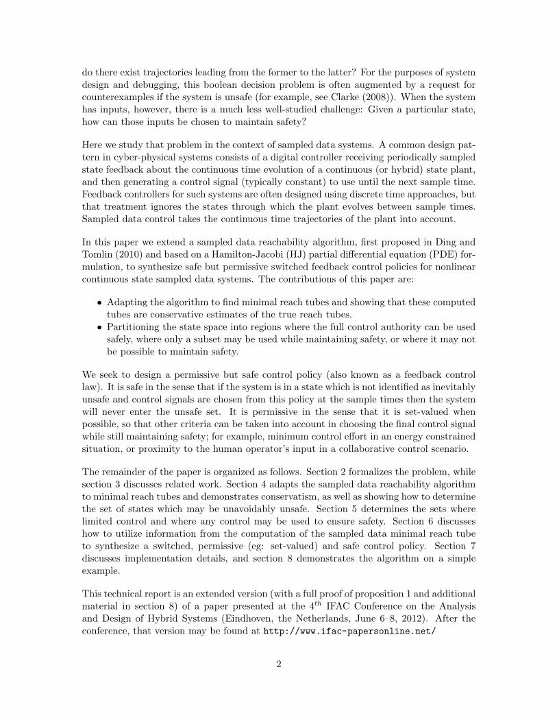
Sctrl Sfree

SN

S0 S1 S2

S3

Figure 1: The partition of the state space. The unsafe set S0 and the state space Ω arespecified in the problem definition. The uncontrollable sets Sk for k > 0, the mandatorycontrol set Sctrl and the free control set Sfree are determined by the algorithms proposed inthis paper.

2 Problem Definition

Consider a deterministic nonlinear system described by the ordinary differential equation(ODE)

x = f(x, u) (1)

with initial condition x(0) = x0, where x ∈ Ω is the state, Ω ⊂ Rdx (or some similar vectorspace of dimension dx), u ∈ U is the control input, U ⊂ Rdu is assumed to be convexand compact, and the dynamics f : Ω × U → TΩ are assumed to be bounded, Lipschitzcontinuous in x, and continuous in u.

We will assume that for feedback control purposes the state is sampled at times tk = kδfor some fixed δ > 0 and integer k, and that the control signal is constant between sampletimes. As a consequence, the actual dynamics are of the form

x(t) = f(x(t), upw(t)) (2)

where the piecewise constant input signal upw(t) is chosen according to

upw(t) = ufb(x(tk)) for tk ≤ t < tk+1 (3)

and ufb : Ω→ U is a feedback control policy. Note that because the feedback control policyis time sampled, the dynamics (2) cannot be written in the form x = f(x).

The unsafe set S0 ⊂ Ω that we seek to avoid is assumed to be the closure of an open set; forexample, it need not be connected, but every unconnected component must have an interiorand an exterior. We divide the state space Ω into a number of subsets as shown in figure 1.

3

The first is the terminal set S0. The next sets Sk may inevitably enter the terminal set bytime kδ no matter what ufb is chosen. The next set Sctrl is a superset of SN—where Nδwill be our safety horizon—and is the set in which we will constrain ufb in order to ensuresafety. The final set Sfree is the set of states in which any ufb may be chosen at the nextsampling instant.

We will determine these sets through a series of reachability calculations. Starting from S0,we determine Sk for k = 1, 2, . . . , N through a sampled time backward minimal reachabilitycalculation. We then use SN as the terminal set in a traditional, continuous time backwardmaximal reachability calculation; Sctrl is the resulting backwards reach tube. Finally, Sfreeis the remainder of the state space.

We represent sets S ⊂ Ω using an implicit surface function ψS : Ω→ R such that

S = x ∈ Ω | ψS(x) ≤ 0.

The implicit surface function representation is very flexible; for example, it can representnonconvex and disconnected sets. Its main restriction is that sets must have a nonemptyinterior and exterior. Analytic implicit surface functions for common geometric shapes(such as spheres, hyperplanes, prisms, etc.) are easily constructed. The constructive solidgeometry operations of union, intersection and complement of sets are achieved throughpointwise minimum, maximum and negation operations on their implicit surface functions.

For notational simplicity, we have restricted the presentation below to the case of a singleinput which is acting as a control. It is straightforward to modify the schemes in the samemanner as Ding and Tomlin (2010) to treat measurable disturbance inputs or hybrid au-tomata dynamics with continuously available mode switches. More extensive modificationswould be required to treat the cases where the disturbance input and/or the mode switcheswere based on sampled data as well.

3 Related Work

We broadly categorize reachability algorithms into Lagrangian (those which follow trajec-tories of the system) and Eulerian (those which operate on a fixed grid); see Mitchell (2007)for a more extensive discussion of types of reachability algorithms. Most algorithms forsystems with nonlinear dynamics and inputs are currently Eulerian; for example, there areschemes based on viability theory (Cardaliaguet et al. (1999); Aubin et al. (2011)), staticHJ PDEs (Branicky and Zhang (2000); Sethian and Vladimirsky (2002)), or time-dependentHJ PDEs (Lygeros et al. (1999); Lygeros (2004); Mitchell et al. (2005)). In the static HJPDE formulation, the value function is constant outside the reachable set; consequently,this formulation is not useful for synthesizing safe controls. Using the viability and time-dependent HJ PDE formulations, it is possible to synthesize control laws that are optimallypermissive: constraints are only placed upon the choice of control along the boundary of thesafe (viable) set. From a practical perspective, such policies are impossible to implementbecause they require information about the state at all times and the ability to change the

4

input signal at any time. In contrast, here we assume that state feedback and control signalmodification only occur at the periodic sample times, and the control signal is held constantbetween sample times.

In Ding and Tomlin (2010) a time-dependent HJ PDE formulation of sampled data reacha-bility is presented for hybrid automata. In that case, the HJ PDE is used to find an implicitsurface representation of the sampled data backward reach tube, where the piecewise con-tinuous control input signal attempted to drive the trajectory to a terminal set withoutentering an avoid set, despite the actions of a measurable disturbance input signal. In thatproblem the terminal set was considered “good” from the viewpoint of the control input,while in the problem we explore here the terminal set is considered “bad.” In section 4 wedescribe the minor adaptation of the algorithm required to handle the different interpre-tation of terminal sets, and then examine the relationship between the resulting HJ PDEsolutions and the desired reachability operators.

An alternative approach for finding safe trajectories is through sample based planningschemes (for example, see LaValle (2006)), such as the rapidly-exploring random tree (RRT)and its descendants. Adaptations of RRTs to verification/falsification are proposed in Bran-icky et al. (2006); Plaku et al. (2009), but to synthesize permissive yet safe control policiesrequires a slightly different but still quite feasible modification of traditional RRTs (to col-lect sets of safe paths, rather than just the optimal or first path found). Like many samplebased schemes RRTs appear to scale better in practice to high dimensional systems thando schemes based on grids, and unlike most Lagrangian approaches they do a good job ofcovering the state space given sufficient samples. On the other hand, the output of RRTsis not as easily or accurately interpolated into continuous spaces as are grid-based results,and there is no simple method of introducing worst-case disturbance inputs to make theresults robust to uncertainty.

4 Sampled Data Reachability

In this section we define a minimal reach tube operator for the sampled data dynamics (2)–(3), show how it can be represented as an implicit surface function constructed from thesolutions of HJ PDEs via some simple pointwise operations, demonstrate its (possibly strict)conservatism, and specify a formula for Sk.

4.1 Minimal Reach Tubes

Define the sampled data backward minimal reach tube over time interval [tmin, tmax] as

R−sd([tmin, tmax], T ) , x0 ∈ Ω | ∀upw(·), ∃t ∈ [tmin, tmax], x(t) ∈ T , (4)

where x(·) solves (2)–(3) with initial condition x(0) = x0. The backward minimal reachtube contains states that give rise to trajectories which cannot avoid entering T no matterwhat input signal is chosen. Note that this definition is not precisely the same as thosein Mitchell (2007) because in this case we allow only piecewise constant control signals.

5

4.2 Hamilton-Jacobi Formulation

We adapt the approach from Ding and Tomlin (2010) to approximate the backward minimalreach tube. A finite subset of control input values U = u(1), u(2), . . . , u(`) is considered,where u(j) ∈ U . Define the backward reach tube for a constant input value u(j) over a singlesample period as

R(j) , R([0, δ], T ) , x0 ∈ Ω | ∃t ∈ [0, δ], x(t) ∈ T

where x(·) solves (1) with fixed input u(j) and initial condition x(0) = x0. If T is representedby the known implicit surface function ψT , then we can determine an implicit surfacefunction for R(j) (for example, see Mitchell et al. (2005))

ψR(j)(x) = φ(x, 0) (5)

where φ : Ω× [0, δ]→ R is the viscosity solution of the terminal value, time-dependent HJPDE

Dtφ+ min [0, H(x,Dxφ)] = 0 (6)

with HamiltonianH(x, p) = pT f(x, u(j)) (7)

and terminal conditionφ(x, δ) = ψT (x). (8)

Unlike Ding and Tomlin (2010), we use the control input to minimize the size of the reachtube, so an implicit surface function for

R−1 (T ) , R−sd([0, δ], T )

is given byψR−1 (T )(x) = max

1≤j≤`ψR(j)(x). (9)

This optimization ensures that if point x is outside R(j) for any j—in other words, inputu(j) generates a trajectory starting at x which does not reach T during the time interval[0, δ]—then x is outside R−1 (T ). Because it is the maximum of continuous functions, ψR−1 (T )is itself continuous.

Given some finite horizon T = Nδ for integer N > 1, we work recursively through

R−k+1(T ) , R−1 (R−k (T ))

ψR−k+1(T )(x) = ψR−1 (R−k (T ))(x)

(10)

and the equations above to find an implicit surface function for R−N (T ).

6

4.3 Conservatism of the Hamilton-Jacobi Reach Tube Formulation

Proposition 1. The true sampled data reach tube is a subset of the estimated reach tubecomputed in section 4.2:

R−sd([0, Nδ], T ) ⊆ x ∈ Ω | ψR−N (T )(x) ≤ 0. (11)

It may be a strict subset.

Proof. We can prove (11) by showing

x ∈ R−sd([0, Nδ], T ) =⇒ ψR−N (T )(x) ≤ 0.

The proof itself is identical to the first part of lemma 8 in Mitchell et al. (2005) and so wedo not repeat it here (all lemmas and the corollary referenced in this proof are from thesame citation). To show that the true reach tube may be a strict subset of the computedtube, we consider the other part of lemma 8, which turns out to be false for the sampleddata case:

ψR−N (T )(x) ≤ 0 =⇒6 x ∈ R−sd([0, Nδ], T ). (12)

The proof of this part of lemma 8 fails because the dynamics (2) depend implicitly on timethrough the sampled control (3), the trajectories of the augmented system can be forcedinto states which are not visited by the original system, and hence lemma 4 and corollary 5are false.

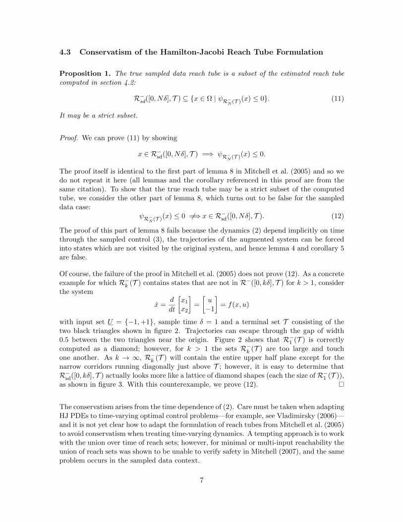
Of course, the failure of the proof in Mitchell et al. (2005) does not prove (12). As a concreteexample for which R−k (T ) contains states that are not in R−([0, kδ], T ) for k > 1, considerthe system

x =d

dt

[x1x2

]=

[u−1

]= f(x, u)

with input set U = −1,+1, sample time δ = 1 and a terminal set T consisting of thetwo black triangles shown in figure 2. Trajectories can escape through the gap of width0.5 between the two triangles near the origin. Figure 2 shows that R−1 (T ) is correctlycomputed as a diamond; however, for k > 1 the sets R−k (T ) are too large and touchone another. As k → ∞, R−k (T ) will contain the entire upper half plane except for thenarrow corridors running diagonally just above T ; however, it is easy to determine thatR−sd([0, kδ], T ) actually looks more like a lattice of diamond shapes (each the size of R−1 (T )),as shown in figure 3. With this counterexample, we prove (12).

The conservatism arises from the time dependence of (2). Care must be taken when adaptingHJ PDEs to time-varying optimal control problems—for example, see Vladimirsky (2006)—and it is not yet clear how to adapt the formulation of reach tubes from Mitchell et al. (2005)to avoid conservatism when treating time-varying dynamics. A tempting approach is to workwith the union over time of reach sets; however, for minimal or multi-input reachability theunion of reach sets was shown to be unable to verify safety in Mitchell (2007), and the sameproblem occurs in the sampled data context.

7

Reach Tube Estimate δ = 1, N = 3

−4 −3 −2 −1 0 1 2 3 4

−0.5

0

0.5

1

1.5

2

2.5

3

3.5

4

Figure 2: A demonstration that R−N (T ) may include states which can avoid hitting theterminal set. The terminal set T is the two black triangles. The remaining shaded regionsare R−k (T ) for k = 1, 2, 3 (darkest to lightest). The blue line shows a trajectory startingfrom within R−2 (T ) which nonetheless avoids the terminal set. The input is sampled at thepoints marked by small circles.

Figure 3: A sketch of the actual R−([0, kδ], T ) for k = 1, 2, 3 for the example in figure 2.

8

4.4 Determining Sk

Using the operators defined above, we (conservatively) determine the set of states that mayinevitably enter S0 over time horizon kδ as

Sk = R−k (S0). (13)

Using (5)–(10) we can determine an implicit surface representation ψSk .

For many problems of interest, we find that this calculation converges such that Sk = Sk−1for sufficiently large k, and hence we can determine the infinite horizon S∞.

5 Continuous Time Maximal Reachability

In order to allow maximum flexibility in the choice of control in Sfree at time t, we mustensure that it contains no states which can give rise to trajectories that enter SN beforethe next state observation and change of input at time t + δ. In this section we recall thestandard maximal reach tube operator and the HJ PDE whose solution provides an implicitsurface representation of this set. We use this operator to determine Sctrl and hence Sfree.

5.1 Maximal Reach Tubes

The backward maximal reach tube for a given terminal set T over time interval [tmin, tmax]is defined as

R+([tmin, tmax], T ) , x0 ∈ Ω | ∃u(·), ∃t ∈ [tmin, tmax], x(t) ∈ T , (14)

where x(·) solves (1) with initial condition x(0) = x0. Note that this definition is exactlythe same as in Mitchell (2007), and we allow for measurable input signals u(·) rather thanthose that are just piecewise constant.

5.2 Hamilton-Jacobi Formulation

We use the algorithm from Mitchell et al. (2005) to determine an implicit surface functionrepresentation of R+([0, δ], T ):

ψR+([0,δ],T )(x) = φ(x, 0),

where φ : Ω× [0, δ]→ R is the viscosity solution of the terminal value, time-dependent HJPDE (6) with Hamiltonian

H(x, p) = minupT f(x, u) (15)

and terminal condition (8).

9

x 2 Sfree

ufb(x) 2 U

x 2 Sctrl

ufb(x) 2 Uctrl(x)

x 2 S1

ufb(x) 2 Uinev(x)

x 2 S0

u is irrelevant to safety

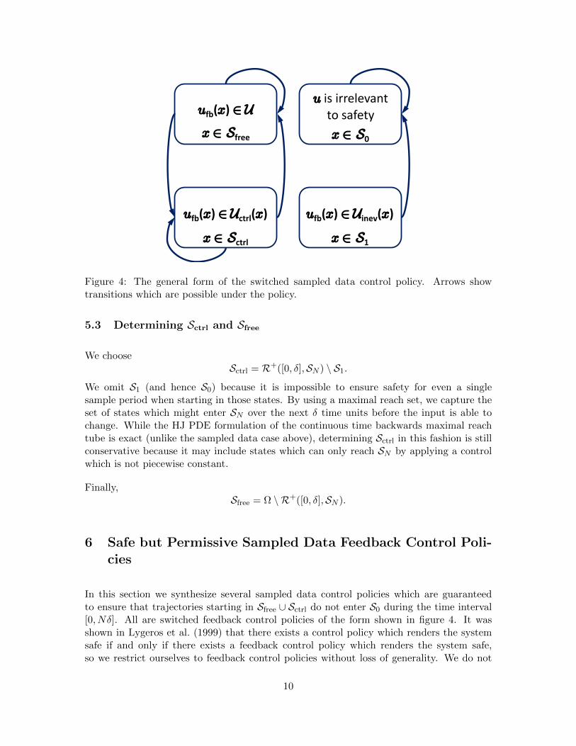
Figure 4: The general form of the switched sampled data control policy. Arrows showtransitions which are possible under the policy.

5.3 Determining Sctrl and Sfree

We chooseSctrl = R+([0, δ],SN ) \ S1.

We omit S1 (and hence S0) because it is impossible to ensure safety for even a singlesample period when starting in those states. By using a maximal reach set, we capture theset of states which might enter SN over the next δ time units before the input is able tochange. While the HJ PDE formulation of the continuous time backwards maximal reachtube is exact (unlike the sampled data case above), determining Sctrl in this fashion is stillconservative because it may include states which can only reach SN by applying a controlwhich is not piecewise constant.

Finally,Sfree = Ω \ R+([0, δ],SN ).

6 Safe but Permissive Sampled Data Feedback Control Poli-cies

In this section we synthesize several sampled data control policies which are guaranteedto ensure that trajectories starting in Sfree ∪ Sctrl do not enter S0 during the time interval[0, Nδ]. All are switched feedback control policies of the form shown in figure 4. It wasshown in Lygeros et al. (1999) that there exists a control policy which renders the systemsafe if and only if there exists a feedback control policy which renders the system safe,so we restrict ourselves to feedback control policies without loss of generality. We do not

10

synthesize a policy for x ∈ S0, since the system has already failed the safety criterion insuch states and so its future evolution is irrelevant to that criterion.

6.1 Policy in Sfree

As shown in figure 4, it is impossible by the construction of Sctrl for the state to go fromSfree to S0 over a single sampling interval no matter what input is chosen. Consequently,the permissive control policy in Sfree is always u ∈ U .

6.2 Policies in Sctrl

For states in Sctrl some choices of input may lead trajectories directly into S0 and othersmay unnecessarily reduce the horizon over which safety can be maintained; consequently,the range of inputs must be constrained. We propose two possible choices of Uctrl(x). Thefirst maximizes permissiveness by providing the largest set of controls which maintainssafety over the maximum possible time horizon. The second aggressively attempts to drivethe trajectory back into Sfree (which might provide more long-term flexibility in choice ofinput). Both choices ensure safety, and are subsets of the finite collection of input samplesU used in constructing the Sk.

Let Nδ be the safety horizon used to compute Sctrl. Given x0 ∈ Sctrl define the safetyhorizon of x0 as

n(x0) ,

∞, if SN = SN−1 = S∞ and ψSN (x0) > 0;

N, if SN 6= SN−1 and ψSN (x0) > 0;

k, if ψSk+1(x0) ≤ 0 and ψSk(x0) > 0.

(16)

Observe that n(x) ≥ 1 because Sctrl does not contain S1. Define the value at the nextsample time under input u(j) ∈ U as

ψ(j)δ (x0) , ψSn(x0)−1

(x(j)(δ)), (17)

where x(j)(·) solves (2) with fixed input u = u(j) and initial condition x(0) = x0.

The permissive policy is given by

U→ctrl(x) , u(j) ∈ U | ψ(j)δ (x) ≥ ψSn(x)

(x). (18)

The aggressive policy is given by

Uctrl(x) , argmaxu(j)∈U

ψ(j)δ (x). (19)

Note that neither policy is guaranteed to be unique.

Proposition 2. For all x ∈ Sctrl, U→ctrl(x) 6= ∅.

11

Proof. The HJ PDE (6)–(8) used to compute ψR(j) and the optimization in (9) implies thatψR−1 (T ) is the value function for the finite horizon terminal value optimal control problem

ψR−1 (T )(x0) = maxu(j)∈U

mins∈[0,δ]

ψT (x(j)(s)) (20)

where x(j)(·) solves (2) with initial condition x(j)(0) = x0 and constant control u(j).

Consider x0 ∈ Sctrl. Let n = n(x0) and ψ = ψSn(x0). By (13) and (10), Sn = R−1 (Sn−1),which implies that

ψR−1 (Sn−1)(x0) = ψSn(x0) = ψ.

Therefore, by (20) there exists ∈ 1, 2, . . . , ` and u() ∈ U such that

mins∈[0,δ]

ψSn−1(x()(s)) = ψ;

consequently, by (17)

ψ()δ (x0) = ψSn−1(x()(δ)) ≥ ψ.

Therefore, u() ∈ U→ctrl(x0).

Corollary 1. For all x ∈ Sctrl, Uctrl(x) 6= ∅. For all u(j) ∈ Uctrl(x), ψ(j)δ (x) ≥ ψSn(x)

(x).

6.3 Policies in S1

For x0 ∈ S1 = R−1 (S0), x(δ) ∈ S0 for all u(j) ∈ U . Furthermore, the computation ofR−1 (S0) does not suffer from the conservatism discussed in proposition 1, because the dy-namics (2)–(3) are not time-dependent over a single sample interval. Consequently, onepossible response is to sit back and wait for the inevitable failure. The corresponding mostpermissive control policy is Uinev(x) , U . However, if there is some conservatism in themodel—for example, if disturbance inputs have been introduced into (2) and treated in aworst-case manner when computing R−1 (S0)—it may be possible to avoid S0. The corre-sponding policy

Uinev(x) , argmaxu(j)∈U

ψS0(x(j)(δ)) (21)

is defined in a manner similar to Uctrl(x), although for x ∈ S1 there is no guarantee thatapplication of this policy will avoid S0 for even a single sample interval.

6.4 Safety of the Policies

Proposition 3. Let trajectory x(·) solve (2)–(3) with initial condition x(0) = x0 and sam-pled feedback control policy

ufb(x) ∈

Uctrl(x), for x ∈ Sctrl;U , for x ∈ Sfree.

(22)

If x0 ∈ Sfree, then x(t) /∈ S0 for all t ∈ [0, (N + 1)δ], where Nδ is the horizon used in thecomputation of Sctrl. If x0 ∈ Sctrl, then x(t) /∈ S0 for all t ∈ [0, n(x0)δ].

12

Proof. Consider first x0 ∈ Sctrl. Let n = n(x0) and ψ = ψSn(x0). By (16), ψ > 0, whichimplies that ψSn−1(x(δ)) > 0 by (17) and either (18) and proposition 2 (if Uctrl = U→ctrl) or

corollary 1 (if Uctrl = Uctrl). Therefore x(δ) /∈ Sn−1. Use induction to show that x(kδ) /∈Sn−k and hence that x(t) /∈ S0 for t ∈ [0, nδ].

Now consider x0 ∈ Sfree, which implies

ψR+([0,δ],SN )(x0) > 0. (23)

The HJ PDE (6), (15) and (8) used to compute ψR+([0,δ],SN ) implies that it is the valuefunction for the finite horizon terminal value optimal control problem

ψR+([0,δ],SN )(x0) = minu(·)∈U

mins∈[0,δ]

ψSN (x(s)) (24)

where x(·) solves (1) with initial condition x(0) = x0 and U is the set of all measurableinput signals u(·) such that u(s) ∈ U for all s ∈ [0, δ]. Note that U is a much broader choiceof input signals than piecewise constant, and it draws values from U not U , so the set ofall possible trajectories x(·) contains all sampled data trajectories x(·). From (23) and (24)we conclude that ψSN (x(s)) > 0 for all s ∈ [0, δ] and hence that either x(δ) ∈ Sfree orx(δ) ∈ Sctrl with n(x(δ)) = N . Using either induction in the former case or the proof abovefor x0 ∈ Sctrl in the latter case, it is easily shown that x(t) /∈ S0 for all t ∈ [0, (N + 1)δ]

Corollary 2. If the sampled data reachability calculation converged such that SN−1 =SN = S∞ and x0 ∈ Sfree ∪ (Sctrl \ S∞), then using the control policy (22) will ensure thatx(t) ∈ Sfree ∪ (Sctrl \ S∞) for all t > 0.

7 Approximation and Implementation

In this section we describe a particular approach to approximating the solution of theequations above for the common case where we do not have analytic solutions to thoseequations.

7.1 Calculating the Sets

We use the Toolbox of Level Set Methods (ToolboxLS) as described in Mitchell andTempleton (2005) to manipulate implicit surface functions. Implicit surface functions arerepresented by values sampled at nodes on a regular orthogonal grid. When values areneeded away from grid points, interpolation is used (eg: interpn in Matlab). Maximumand minimum operations are done pointwise at each node in the grid.

The HJ PDE (6)–(8) used to determine Sk is purely convective because there are no inputs;consequently, it can be solved using an upwind finite difference scheme. High order ofaccuracy finite difference approximations of the spatial and temporal derivatives are usedto evolve the equation (for example, see Osher and Fedkiw (2002)). However, because we

13

use the value of ψSk , and not just its zero level set, during construction of the controlpolicies (via (17)), it is important that reinitialization and/or velocity extension not beapplied when approximating the solution of these PDEs.

The HJ PDE (6), (15) and (8) used to determine Sctrl involves an input, so a Lax-Friedrichscentered difference scheme is used. The same spatial and temporal finite difference approx-imations are used. Only the zero level set of ψSctrl is referenced, so it is possible to usereinitialization and/or velocity extension during this process; however, it is unlikely to beneeded because the equations are solved only over δ time units.

7.2 Constructing the Feedback Controller

For a state x0 ∈ Sfree ∪ S0 the control policies are straightforward to implement. Forx0 ∈ Sctrl, we approximate (17) for each j = 1, 2, . . . , ` by using an ODE solver (eg:ode45 in Matlab) to find the point x(j)(δ) and then interpolate over the approximation

of ψSn(x0)−1to determine ψ

(j)δ (x0). The set-valued policy is constructed from (18) or (19),

where ψSn(x0)(x0) might also need to be interpolated in (18).

7.3 Guaranteeing an Overapproximation

While the analytic formulation presented in sections 4–6 guarantees safety, the numericalimplementation described above does not maintain those guarantees. The decision to usean unsound implementation was primarily driven by convenience, and also the empiricalaccuracy that the level set schemes have demonstrated in the past.

It is possible to reformulate the reachability calculations described above in viability theoryand then use sound numerical implementations such as those described in Cardaliaguetet al. (1999). The sampled data minimal reachability calculation in section 4 is solvedby a series of fixed input reachability calculations with switches at the sample times, butcould also be solved by a series of fixed input viability kernels with switches at the sampletimes. The maximal reachability calculation in section 5 can be solved with a capturebasin. It is less obvious how to synthesize safe controls from the indicator-like viabilitykernel representation, but there are several approaches to reformulate HJ PDEs as viabilitykernels if necessary. The primary shortcoming of these viability schemes is their relativeinaccuracy when compared to the schemes implemented in ToolboxLS. It is possible thata combination of the two approaches might be able to achieve both sound and accurateapproximations.

8 Example

Computations were done on an Intel Core2 Duo at 1.87 GHz with 4 GB RAM running64-bit Windows 7 Professional (Service Pack 1), 64-bit Matlab version 7.11 (R2010b),

14

delta = 0.30, steps = 50, |u| ≤ 1.00, input samples = 7, accuracy veryHigh

−5 −4 −3 −2 −1 0 1 2 3 4 5−2.5

−2

−1.5

−1

−0.5

0

0.5

1

1.5

2

2.5

unsafeinevitablecontrol

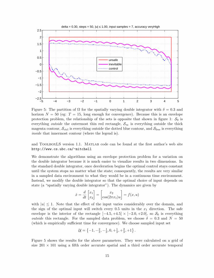
Figure 5: The partition of Ω for the spatially varying double integrator with δ = 0.3 andhorizon N = 50 (eg: T = 15, long enough for convergence). Because this is an envelopeprotection problem, the relationship of the sets is opposite that shown in figure 1: S0 iseverything outside the outermost thin red rectangle, S∞ is everything outside the thickmagenta contour, Sctrl is everything outside the dotted blue contour, and Sfree is everythinginside that innermost contour (where the legend is).

and ToolboxLS version 1.1. Matlab code can be found at the first author’s web sitehttp://www.cs.ubc.ca/~mitchell

We demonstrate the algorithms using an envelope protection problem for a variation onthe double integrator because it is much easier to visualize results in two dimensions. Inthe standard double integrator, once deceleration begins the optimal control stays constantuntil the system stops no matter what the state; consequently, the results are very similarin a sampled data environment to what they would be in a continuous time environment.Instead, we modify the double integrator so that the optimal choice of input depends onstate (a “spatially varying double integrator”). The dynamics are given by

x =d

dt

[x1x2

]=

[x2

cos(2πx1)u

]= f(x, u)

with |u| ≤ 1. Note that the effect of the input varies considerably over the domain, andthe sign of the optimal input will switch every 0.5 units in the x1 direction. The safeenvelope is the interior of the rectangle [−4.5,+4.5] × [−2.0,+2.0], so S0 is everythingoutside this rectangle. For the sampled data problem, we choose δ = 0.3 and N = 50(which is empirically sufficient time for convergence). We choose sampled input set

U =−1,−2

3 ,−13 , 0,+

13 ,+

23 ,+1

.

Figure 5 shows the results for the above parameters. They were calculated on a grid ofsize 201 × 101 using a fifth order accurate spatial and a third order accurate temporal

15

Figure 6: The effect of δ on the spatial partition. Top: Traditional reachability withcontinuous state feedback and measurable control signals (T = 4). Middle: Sampled datawith δ = 0.1, N = 40 (T = 4). Bottom: Sampled data with δ = 1.0, N = 24 (T = 24).

16

derivative approximation. Figure 6 shows results for the continuous time version, and alsofor versions with δ = 0.1 and δ = 1.0. Notice that the continuous time version has a muchlarger Sfree because it can always choose an input that generates deceleration. Furthermore,Sctrl = S∞ in this case, because δ = 0. In contrast, as δ becomes large the envelope becomesincreasingly uncontrollable.

Figures 7 and 8 show some sample trajectories generated using the policy (22) with U→ctrl and

Uctrl respectively. For illustrative purposes the control was chosen to drive the trajectoryback toward Sctrl for x ∈ Sfree, and was chosen for U→ctrl to keep the trajectory as deeplywithin Sctrl as possible, but other choices are available. In the bottom of each plot, noticethat the value of ψS∞ may decrease along a trajectory between samples, but if the trajectoryis in Sctrl (as indicated by the blue dots) at the sample time, then the value of ψS∞ doesnot decrease at the subsequent sample time.

9 Conclusions and Future Work

We have adapted the sampled data reachability algorithm from Ding and Tomlin (2010) toa safety maintenance / viability problem, and demonstrated how the algorithm computes aconservative estimate of the sampled data backward reach tube. We have then demonstratedhow to synthesize a permissive but safe control policy from this calculation, which may haveapplications in multi-objective or collaborative control problems. In the future we plan toapply this scheme to more complex nonlinear and hybrid systems with disturbance inputs,taking into account model, state, and discretization uncertainty.

References

Jean-Pierre Aubin, Alexandre M. Bayen, and Patrick Saint-Pierre. Viability Theory: NewDirections. Systems & Control: Foundations & Applications. Springer, 2011. doi: 10.1007/978-3-642-16684-6.

Michael S. Branicky and Gang Zhang. Solving hybrid control problems: Level sets andbehavioral programming. In Proceedings of the American Control Conference, pages1175–1180, Chicago, IL, 2000.

M.S. Branicky, M.M. Curtiss, J. Levine, and S. Morgan. Sampling-based planning, controland verification of hybrid systems. IEE Proceedings Control Theory and Applications,153(5):575 – 590, 2006.

P. Cardaliaguet, M. Quincampoix, and P. Saint-Pierre. Set-valued numerical analysisfor optimal control and differential games. In M. Bardi, T. E. S. Raghavan, andT. Parthasarathy, editors, Stochastic and Differential Games: Theory and NumericalMethods, volume 4 of Annals of International Society of Dynamic Games, pages 177–247.Birkhauser, 1999.

17

−5 −4 −3 −2 −1 0 1 2 3 4 5−2.5

−2

−1.5

−1

−0.5

0

0.5

1

1.5

2

2.5

x1

x 2

Reach setDonut setInitial pointsTrajectories

0 0.5 1 1.5 2 2.5 30

0.5

1

1.5

2

t

func

tion

valu

e

Figure 7: Sample trajectories using the permissive safe policy U→ctrl for δ = 0.3. Top: Tra-jectories x(·) in phase space overlaid on the state space partition. Bottom row: ψS∞(x(t))versus t. Sample times are shown as red circles, and periods during which x(t) ∈ Sctrl areshown with blue dots.

18

−5 −4 −3 −2 −1 0 1 2 3 4 5−2.5

−2

−1.5

−1

−0.5

0

0.5

1

1.5

2

2.5

x1

x 2

Reach setDonut setInitial pointsTrajectories

0 0.5 1 1.5 2 2.5 30

0.5

1

1.5

2

t

func

tion

valu

e

Figure 8: Sample trajectories using the aggressive safe policy Uctrl for δ = 0.3. Top: Tra-jectories x(·) in phase space overlaid on the state space partition. Bottom row: ψS∞(x(t))versus t. Sample times are shown as red circles, and periods during which x(t) ∈ Sctrl areshown with blue dots.

19

Edmund M. Clarke. The birth of model checking. In Orna Grumberg and Helmut Veith,editors, 25 Years of Model Checking, number 5000 in Lecture Notes in Computer Science,pages 1–26. Springer Verlag, 2008. doi: 10.1007/978-3-540-69850-0 1.

Jerry Ding and Claire J. Tomlin. Robust reach-avoid controller synthesis for switchednonlinear systems. In Proceedings of the IEEE Conference on Decision and Control,pages 6481–6486, Atlanta, GA, 2010. doi: 10.1109/CDC.2010.5717115.

Steven M. LaValle. Planning Algorithms. Cambridge University Press, New York, 2006.

John Lygeros. On reachability and minimum cost optimal control. Automatica, 40(6):917–927, 2004. doi: 10.1016/j.automatica.2004.01.012.

John Lygeros, Claire Tomlin, and Shankar Sastry. Controllers for reachability specifica-tions for hybrid systems. Automatica, 35(3):349–370, 1999. doi: 10.1016/S0005-1098(98)00193-9.

Ian M. Mitchell. Comparing forward and backward reachability as tools for safety analysis.In Alberto Bemporad, Antonio Bicchi, and Giorgio Buttazzo, editors, Hybrid Systems:Computation and Control, number 4416 in Lecture Notes in Computer Science, pages428–443. Springer Verlag, 2007. doi: 10.1007/978-3-540-71493-4 34.

Ian M. Mitchell and Jeremy A. Templeton. A toolbox of Hamilton-Jacobi solversfor analysis of nondeterministic continuous and hybrid systems. In Manfred Morariand Lothar Thiele, editors, Hybrid Systems: Computation and Control, number 3414in Lecture Notes in Computer Science, pages 480–494. Springer Verlag, 2005. doi:10.1007/978-3-540-31954-2 31.

Ian M. Mitchell, Alexandre M. Bayen, and Claire J. Tomlin. A time-dependent Hamilton-Jacobi formulation of reachable sets for continuous dynamic games. IEEE Transactionson Automatic Control, 50(7):947–957, 2005. doi: 10.1109/TAC.2005.851439.

Stanley Osher and Ronald Fedkiw. Level Set Methods and Dynamic Implicit Surfaces.Springer, 2002. doi: 10.1007/b98879.

Erion Plaku, Lydia Kavraki, and Moshe Vardi. Hybrid systems: from verification to falsi-fication by combining motion planning and discrete search. Formal Methods in SystemDesign, 34:157–182, 2009. doi: 10.1007/s10703-008-0058-5.

James A. Sethian and Alexander Vladimirsky. Ordered upwind methods for hybrid control.In C. J. Tomlin and M. R. Greenstreet, editors, Hybrid Systems: Computation and Con-trol, number 2289 in Lecture Notes in Computer Science, pages 393–406. Springer Verlag,2002.

Alexander Vladimirsky. Static PDEs for time-dependent control problems. Interfaces andFree Boundaries, 8(3):281–300, 2006. doi: 10.4171/IFB/144.

20