enterpriseone jde5 forecasting peoplebook - oracle · enterpriseone jde5 forecasting peoplebook ......
TRANSCRIPT
EnterpriseOne JDE5ForecastingPeopleBook
May 2002

EnterpriseOne JDE5Forecasting PeopleBook SKU JDE5EFC0502 Copyright© 2003 PeopleSoft, Inc. All rights reserved. All material contained in this documentation is proprietary and confidential to PeopleSoft, Inc. ("PeopleSoft"), protected by copyright laws and subject to the nondisclosure provisions of the applicable PeopleSoft agreement. No part of this documentation may be reproduced, stored in a retrieval system, or transmitted in any form or by any means, including, but not limited to, electronic, graphic, mechanical, photocopying, recording, or otherwise without the prior written permission of PeopleSoft. This documentation is subject to change without notice, and PeopleSoft does not warrant that the material contained in this documentation is free of errors. Any errors found in this document should be reported to PeopleSoft in writing. The copyrighted software that accompanies this document is licensed for use only in strict accordance with the applicable license agreement which should be read carefully as it governs the terms of use of the software and this document, including the disclosure thereof. PeopleSoft, PeopleTools, PS/nVision, PeopleCode, PeopleBooks, PeopleTalk, and Vantive are registered trademarks, and Pure Internet Architecture, Intelligent Context Manager, and The Real-Time Enterprise are trademarks of PeopleSoft, Inc. All other company and product names may be trademarks of their respective owners. The information contained herein is subject to change without notice. Open Source Disclosure This product includes software developed by the Apache Software Foundation (http://www.apache.org/). Copyright (c) 1999-2000 The Apache Software Foundation. All rights reserved. THIS SOFTWARE IS PROVIDED “AS IS’’ AND ANY EXPRESSED OR IMPLIED WARRANTIES, INCLUDING, BUT NOT LIMITED TO, THE IMPLIED WARRANTIES OF MERCHANTABILITY AND FITNESS FOR A PARTICULAR PURPOSE ARE DISCLAIMED. IN NO EVENT SHALL THE APACHE SOFTWARE FOUNDATION OR ITS CONTRIBUTORS BE LIABLE FOR ANY DIRECT, INDIRECT, INCIDENTAL, SPECIAL, EXEMPLARY, OR CONSEQUENTIAL DAMAGES (INCLUDING, BUT NOT LIMITED TO, PROCUREMENT OF SUBSTITUTE GOODS OR SERVICES; LOSS OF USE, DATA, OR PROFITS; OR BUSINESS INTERRUPTION) HOWEVER CAUSED AND ON ANY THEORY OF LIABILITY, WHETHER IN CONTRACT, STRICT LIABILITY, OR TORT (INCLUDING NEGLIGENCE OR OTHERWISE) ARISING IN ANY WAY OUT OF THE USE OF THIS SOFTWARE, EVEN IF ADVISED OF THE POSSIBILITY OF SUCH DAMAGE. PeopleSoft takes no responsibility for its use or distribution of any open source or shareware software or documentation and disclaims any and all liability or damages resulting from use of said software or documentation.

Table of Contents
Overviews 1 Industry Overview.................................................................................................... 1 Forecasting Overview.............................................................................................. 3
Detail Forecasts 17 Setting Up Detail Forecasts..................................................................................... 17 Working with Sales Order History............................................................................ 26 Working with Detail Forecasts ................................................................................. 35
Summary Forecasts 68 Setting Up Summary Forecasts............................................................................... 72 Summarizing Detail Forecasts................................................................................. 83 Working with Summarized Detail Forecasts............................................................ 87 Generating Summary Forecasts.............................................................................. 96
Working with Planning Bill Forecasts 122 Working with Planning Bill Forecasts ..............................................................122
Planning Bill Forecasts ............................................................................................ 122 Setting Up a Planning Bill ........................................................................................ 125 Generating Planning Bill Forecasts ......................................................................... 132
Working With Forecasting Interoperability 135
Appendices 136 Forecast Calculation Methods.........................................................................136
Historical Sales Data ............................................................................................... 136 Forecast Performance Evaluation Criteria .............................................................. 136 Evaluating the Forecasts ......................................................................................... 151

Overviews
The Forecasting system allows you to effectively manage customer demand with timely, reliable forecasts. Understanding the importance of forecasts can help you plan and manage your forecasts to suit your specific business needs.
Industry Overview
To understand the critical role that forecasts play in the business environment, you must be aware of the different types of forecasts and the data used to create these forecasts.
Industry Environment and Concepts for Forecasting
Forecasting has grown beyond the simple prediction of future sales based on data from previous years. The globalization of businesses has created a need for multiple forecasts by area, revision level, and perhaps even by key customer.
Now more than ever, businesses must be able to quickly create multiple scenarios for instant evaluation in making informed planning decisions. Businesses require the ability to build customer or item forecasts at the detail and aggregate level with algorithms that reflect product demand patterns. It's imperative that companies can proactively plan and manage forecasts with the flexibility needed for specific business requirements.
Topics Forecasting methods
Multilevel forecasting
Demand forecasting
Simplifying the forecast
Measuring accuracy
Integrating information
Forecasting Methods Overview
To stay competitive, companies need to build realistic forecasts based on their organization's unique business practices. For example, to match market patterns, companies require the ability to use multiple industry-standard forecast algorithms for quantitative or intrinsic forecasting, including the following values:
• Seasonal
• Weighted average
• Exponential smoothing
• Percent over last year
• Calculated percent over last year
• Last year to this year
• Moving average
• Linear approximation
• Least square regression
1
• Second degree approximation
• Flexible method
• Linear smoothing
Using these industry-standard forecasting equations, businesses need their system to calculate the percentage of accuracy for the "best fit" forecast, normally using Mean Absolute Deviation (MAD), according to current and historical demand information.
Businesses also require the ability to revise the data that is included in their forecast. For example, a business might include data that is not typical. To forecast more accurately, the data must be revised. Another example for this revision capability requirement is the need to insert data that was not captured in the past because of some unpredictable on-hand information.
Forecasting uses the Qualitative technique. It uses subjective projections based on judgment, intuition, and informed opinions. Extrinsic techniques, using economic indicators, are also necessary methods in calculating a forecast. For example, an economic indicator can be the amount of disposable income, which affects demand.
Companies that want to keep up-to-date must have the ability to develop hypothetical scenarios using the different forecasting methods and techniques.
Multilevel Forecasting
Businesses require the ability to forecast at any level. For example, they might need to generate either detail forecasts (single-item) or summary forecasts that reflect product line demand patterns. They might need to forecast at the company, department, item group, or at a specific item level.
Demand Forecasting
In today's customer-focused environment, businesses need to create separate forecasts for major customers or customer groups in order to isolate key demand sources. Demand forecasting is essential in a customer-driven environment. Coordination between planning by the Operations department, through materials management, and meeting customer needs by the Marketing department is the key to recognizing and managing product demand.
Integrating Information
Companies need integration within their supply chain. The ability to access all pertinent information for accurate forecasting and planning is imperative. Systems need to talk to each other to facilitate decision-making and planning. This integration eases the process of obtaining the necessary information to generate an accurate forecast.
Simplifying the Forecast
To simplify the forecast process, companies generally use a Planning Bill. Planning Bills are an artificial grouping of components, or bills of material, used for planning purposes. For example, if there are 24 different bills of material, based on different end products, the 24 bills can show the percentage split for each type of component on one bill.
Measuring Accuracy
Forecast error due to bias, which is the difference between actual demand and forecast demand, needs to be calculated to make more informed forecasting decisions. One commonly used method for measuring error is MAD. MAD is calculated by dividing the sum of absolute deviations by the number of total observations.
2
Forecasting Overview
Effective management of distribution and manufacturing activities begins with understanding and anticipating market needs. Forecasting is the process of projecting past sales demand into the future. Implementing a forecasting system allows you to quickly assess current market trends and sales so that you can make informed decisions about your operations.
You can use forecasts to make planning decisions about:
• Customer orders
• Inventory
• Delivery of goods
• Work load
• Capacity requirements
• Warehouse space
• Labor
• Equipment
• Budgets
• Development of new products
• Work force requirements
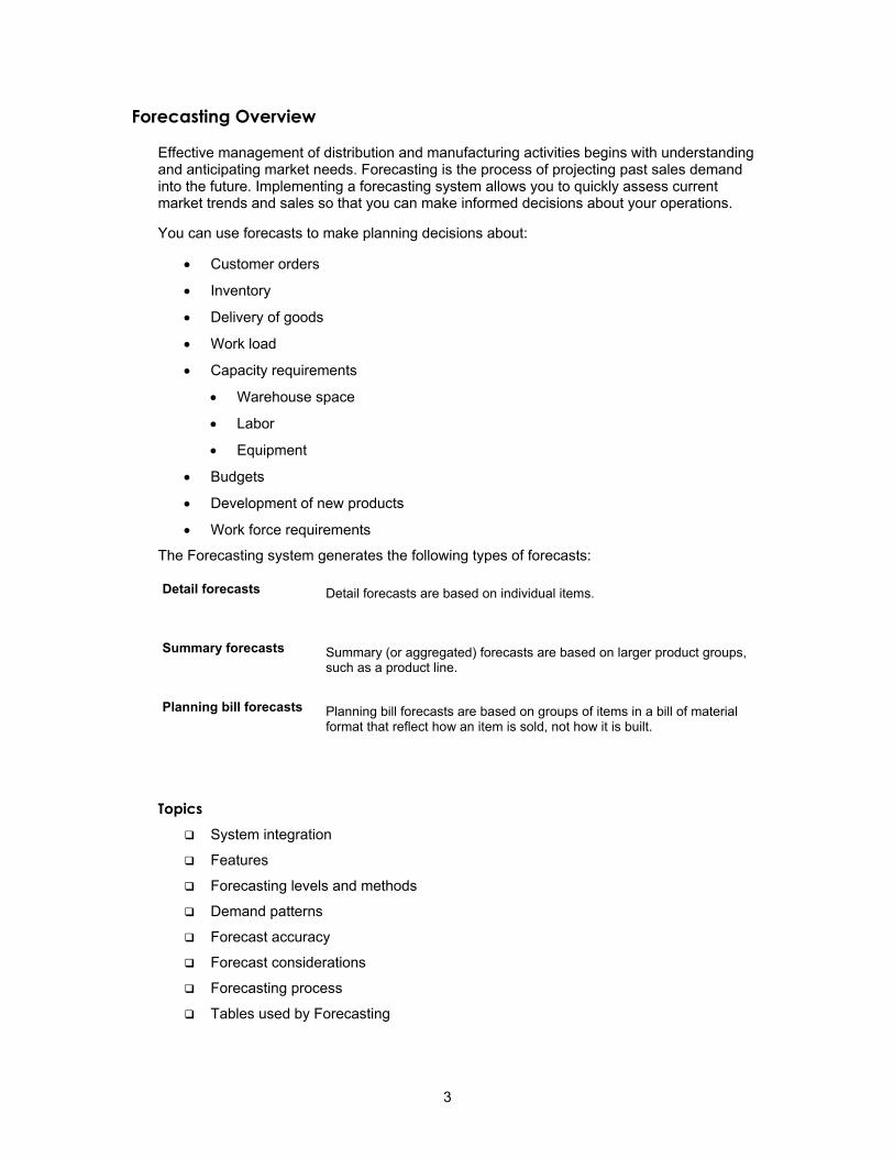
The Forecasting system generates the following types of forecasts:
Detail forecasts
Detail forecasts are based on individual items.
Summary forecasts
Summary (or aggregated) forecasts are based on larger product groups, such as a product line.
Planning bill forecasts
Planning bill forecasts are based on groups of items in a bill of material format that reflect how an item is sold, not how it is built.
Topics System integration
Features
Forecasting levels and methods
Demand patterns
Forecast accuracy
Forecast considerations
Forecasting process
Tables used by Forecasting
3
System Integration
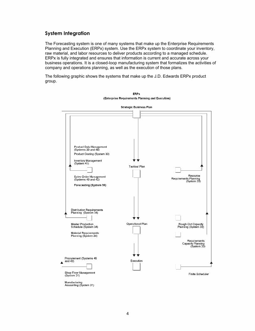
The Forecasting system is one of many systems that make up the Enterprise Requirements Planning and Execution (ERPx) system. Use the ERPx system to coordinate your inventory, raw material, and labor resources to deliver products according to a managed schedule. ERPx is fully integrated and ensures that information is current and accurate across your business operations. It is a closed-loop manufacturing system that formalizes the activities of company and operations planning, as well as the execution of those plans.
The following graphic shows the systems that make up the J.D. Edwards ERPx product group.
4
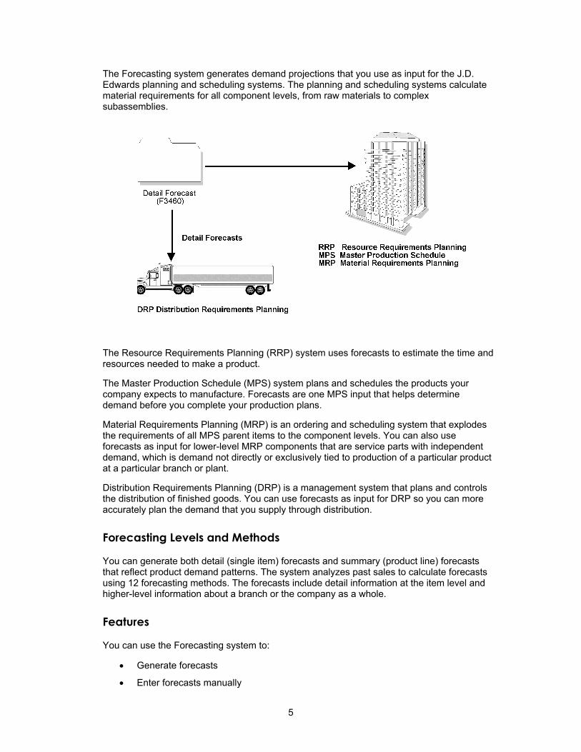
The Forecasting system generates demand projections that you use as input for the J.D. Edwards planning and scheduling systems. The planning and scheduling systems calculate material requirements for all component levels, from raw materials to complex subassemblies.
The Resource Requirements Planning (RRP) system uses forecasts to estimate the time and resources needed to make a product.
The Master Production Schedule (MPS) system plans and schedules the products your company expects to manufacture. Forecasts are one MPS input that helps determine demand before you complete your production plans.
Material Requirements Planning (MRP) is an ordering and scheduling system that explodes the requirements of all MPS parent items to the component levels. You can also use forecasts as input for lower-level MRP components that are service parts with independent demand, which is demand not directly or exclusively tied to production of a particular product at a particular branch or plant.
Distribution Requirements Planning (DRP) is a management system that plans and controls the distribution of finished goods. You can use forecasts as input for DRP so you can more accurately plan the demand that you supply through distribution.
Forecasting Levels and Methods
You can generate both detail (single item) forecasts and summary (product line) forecasts that reflect product demand patterns. The system analyzes past sales to calculate forecasts using 12 forecasting methods. The forecasts include detail information at the item level and higher-level information about a branch or the company as a whole.
Features
You can use the Forecasting system to:
• Generate forecasts
• Enter forecasts manually
5
• Maintain both manually entered forecasts and forecasts generated by the system
• Create unique forecasts by large customer
• Summarize sales order history data in weekly or monthly time periods
• Generate forecasts based on any or all of 12 different formulas that address a variety of forecast situations you might encounter
• Calculate which of the 12 formulas provides the best fit forecast
• Define the hierarchy that the system uses to summarize sales order histories and detail forecasts
• Create multiple hierarchies of address book category codes and item category codes, which you can use to sort and view records in the detail forecast table
• Review and adjust both forecasts and sales order actuals at any level of the hierarchy
• Integrate the detail forecast records into DRP, MPS, and MRP generations
• Force changes made at any component level to both higher levels and lower levels
• Set a bypass flag to prevent changes generated by the force program being made to a level
• Store and display both original and adjusted quantities and amounts
• Attach descriptive text to a forecast at the detail and summary levels
Flexibility is a key feature of the J.D. Edwards Forecasting system. The most accurate forecasts take into account quantitative information, such as sales trends and past sales order history, as well as qualitative information, such as changes in trade laws, competition, and government. The system processes quantitative information and allows you to adjust it with qualitative information. When you aggregate, or summarize, forecasts, the system uses changes that you make at any level of the forecast to automatically update all other levels.
You can perform simulations based on the initial forecast to compare different situations. After you accept a forecast, the system updates your manufacturing and distribution plan with any changes you have made.
The system writes zero or negative detail records. For example, if the quantities or amounts in Extract Sales Order History, Detail Forecast Generation, or Enter/Change Actuals are zero or negative, the system creates zero or negative records in the Forecast table (F3460).
Best Fit
The system recommends the best fit forecast by applying the selected forecasting methods to past sales order history and comparing the forecast simulation to the actual history. When you generate a best fit forecast, the system compares actual sales order histories to forecasts for a specific time period and computes how accurately each different forecasting method predicted sales. Then, the system recommends the most accurate forecast as the best fit.
MAD is the mean of the absolute values of the deviations between actual and forecast data. It is a measure of the average magnitude of errors to expect, given a forecasting method and data history.
The system uses the following sequence of steps to determine the best fit:
1. Use each specified method to simulate a forecast for the holdout period.
2. Compare actual sales to the simulated forecasts for the holdout period.
6
3. Calculate the percentage of accuracy or the MAD to determine which forecasting method most closely matched the past actual sales. The system uses either the percentage of accuracy or the MAD based on the processing options that you choose.
4. Recommend a best fit forecast by the percentage of accuracy that is closest to 100 percent (over or under) or the MAD that is closest to zero.
Forecasting Methods
The Forecasting system uses 12 methods for quantitative forecasting and indicates which method provides the best fit for your forecasting situation. Specify the method that you want the system to use in the processing options for the Create Detail Forecast program (P34650).
Method 1 -
Percent Over Last Year
This method uses the Percent Over Last Year formula to multiply each forecast period by the specified percentage increase or decrease.
To forecast demand, this method requires the number of periods for the best fit plus one year of sales history. This method is useful to forecast demand for seasonal items with growth or decline.
Method 2 -
Calculated Percent Over Last Year
This method uses the Calculated Percent Over Last Year formula to compare the past sales of specified periods to sales from the same periods of the previous year. The system determines a percentage increase or decrease, then multiplies each period by the percentage to determine the forecast.
To forecast demand, this method requires the number of periods of sales order history plus one year of sales history. This method is useful to forecast short-term demand for seasonal items with growth or decline.
Method 3 -
Last Year to This Year
This method uses last year's sales for the following year's forecast.
To forecast demand, this method requires the number of periods best fit plus one year of sales order history. This method is useful to forecast demand for mature products with level demand or seasonal demand without a trend.
Method 4 -
Moving Average
This method uses the Moving Average formula to average the specified number of periods to project the next period. You should recalculate it often (monthly or at least quarterly) to reflect changing demand level.
To forecast demand, this method requires the number of periods best fit plus the number of periods of sales order history. This method is useful to forecast demand for mature products without a trend.
Method 5 -
Linear Approximation
This method uses the Linear Approximation formula to compute a trend from the number of periods of sales order history and to project this trend to the forecast. You should recalculate the trend monthly to detect changes in trends.
This method requires the number of periods best fit plus the number of specified periods of the sales order history. This method is useful to forecast demand for new products or products with consistent positive or negative trends that are not due to seasonal fluctuations.
Method 6 -
Least Square Regression (LSR)
This method derives an equation describing a straight-line relationship between the historical sales data and the passage of time. LSR fits a line to the selected range of data such that the sum of the squares of the differences between the actual sales data points and the regression line are minimized. The forecast is a projection of this straight line into the future.
7
This method requires sales data history for the period represented by the number of periods best fit plus the specified number of historical data periods. The minimum requirement is two historical data points. This method is useful to forecast demand when there is a linear trend in the data.
Method 7 -
Second Degree Approximation
To project the forecast, this method uses the Second Degree Approximation formula to plot a curve based on the number of periods of sales history.
This method requires the number of periods best fit plus the number of periods of sales order history times three. This method is not useful to forecast demand for long-term.
Method 8 -
Flexible Method (Percent Over n Months Prior)
This method allows you to select the number of periods best fit block of sales order history that starts n months prior and to apply a percentage increase or decrease with which to modify it. This method is similar to Method 1, Percent Over Last Year, except that you can specify the number of periods that you use as the base.
Depending on what you select as n, this method requires the number of periods best fit plus the number of periods of sales data indicated. This method is useful to forecast demand for a planned trend.
Method 9 -
Weighted Moving Average
The Weighted Moving Average formula is similar to Method 4, Moving Average formula, because it averages the previous month's sales history to project the next month's sales history. With this formula, however, you can assign weights for each prior period.
This method requires the number of weighted periods selected plus the number of periods best fit data. Similar to Moving Average, this method lags behind demand trends, so it is not recommended for products with strong trends or seasonality. This method is useful to forecast demand for mature products with demand that is relatively level.
Method 10 -
Linear Smoothing
This method calculates a weighted average of past sales data. In the calculation, this method uses the number of periods of sales order history (from 1 to 12) indicated in the processing option. The system uses a mathematical progression to weigh data in the range from the first (least weight) to the final (most weight). Then, the system projects this information to each period in the forecast.
This method requires the month's best fit plus the sales order history for the number of periods specified in the processing option.
Method 11 -
Exponential Smoothing
This method calculates a smoothed average, which becomes an estimate representing the general level of sales over the selected historical data periods.
This method requires sales data history for the time period represented by the number of periods best fit plus the number of historical data periods specified. The minimum requirement is two historical data periods. This method is useful to forecast demand when there is no linear trend in the data.
Method 12 -
Exponential Smoothing with Trend and Seasonality
This method calculates a trend, a seasonal index, and an exponentially smoothed average from the sales order history. The system then applies a projection of the trend to the forecast and adjusts for the seasonal index.
This method requires the number of periods best fit plus two years of sales data, and is useful for items that have both trend and seasonality in the forecast. You can enter the alpha and beta factor or have the system calculate them. Alpha and beta factors are the smoothing constant that the system uses to calculate the smoothed average for the general level or magnitude of sales (alpha) and the trend component of the forecast (beta).
8
• Method 1 - Percent Over Last Year
• Method 2 - Calculated Percent Over Last Year
• Method 3 - Last Year to This Year
• Method 4 - Moving Average
• Method 5 - Linear Approximation
• Method 6 - Least Square Regression
• Method 7 - Second Degree Approximation
• Method 8 - Flexible Method
• Method 9 - Weighted Moving Average
• Method 10 - Linear Smoothing
• Method 11 - Exponential Smoothing
• Method 12 - Exponential Smoothing with Trend and Seasonality
Method 1 - Percent Over Last Year This method uses the Percent Over Last Year formula to multiply each forecast period by the specified percentage increase or decrease.
To forecast demand, this method requires the number of periods for the best fit plus one year of sales history. This method is useful to forecast demand for seasonal items with growth or decline.
Method 2 - Calculated Percent Over Last Year This method uses the Calculated Percent Over Last Year formula to compare the past sales of periods specified to sales from the same periods of the previous year. The system determines a percentage increase or decrease, then multiplies each period by the percentage to determine the forecast.
To forecast demand, this method requires the number of periods of sales order history plus one year of sales history. This method is useful to forecast short-term demand for seasonal items with growth or decline.
Method 3 - Last Year to This Year This method uses last year's sales for the following year's forecast.
To forecast demand, this method requires the number of periods best fit plus one year of sales order history. This method is useful to forecast demand for mature products with level demand or seasonal demand without a trend.
Method 4 - Moving Average This method uses the Moving Average formula to average the specified number of periods to project the next period. You should recalculate it often (monthly or at least quarterly) to reflect changing demand level.
To forecast demand, this method requires the number of periods best fit plus the number of periods of sales order history. This method is useful to forecast demand for mature products without a trend.
9
Method 5 - Linear Approximation This method uses the Linear Approximation formula to compute a trend from the number of periods of sales order history and to project this trend to the forecast. You should recalculate the trend monthly to detect changes in trends.
This method requires the number periods best fit plus the number of specified periods of sales order history. This method is useful to forecast demand for new products or products with consistent positive or negative trends that are not due to seasonal fluctuations.
Method 6 - Least Square Regression This method derives an equation describing a straight-line relationship between the historical sales data and the passage of time. LSR fits a line to the selected range of data such that the sum of the squares of the differences between the actual sales data points and the regression line are minimized. The forecast is a projection of this straight line into the future.
This method requires sales data history for the period represented by the number of periods best fit plus the specified number of historical data periods. The minimum requirement is two historical data points. This method is useful to forecast demand when there is a linear trend in the data.
Method 7 - Second Degree Approximation To project the forecast, this method uses the Second Degree Approximation formula to plot a curve based on the number of periods of sales history.
This method requires the number periods best fit plus the number of periods of sales order history times three. This method is not useful to forecast demand for long-term.
Method 8 - Flexible Method This method allows you to select the number of periods best fit block of sales order history that starts n months prior and to apply a percentage increase or decrease with which to modify it. This method is similar to Method 1, Percent Over Last Year, except that you can specify the number of periods that you use as the base.
Depending on what you select as n, this method requires periods best fit plus the number of periods of sales data indicated. This method is useful to forecast demand for a planned trend.
Method 9 - Weighted Moving Average The Weighted Moving Average formula is similar to Method 4, Moving Average formula, because it averages the previous month's sales history to project the next month's sales history. However, with this formula you can assign weights for each of the prior periods.
This method requires the number of weighted periods selected plus the number of periods best fit data. Similar to Moving Average, this method lags behind demand trends, so it is not recommended for products with strong trends or seasonality. This method is useful to forecast demand for mature products with demand that is relatively level.
Method 10 - Linear Smoothing This method calculates a weighted average of past sales data. In the calculation, this method uses the number of periods of sales order history (from 1 to 12) indicated in the processing option. The system uses a mathematical progression to weigh data in the range from the first (least weight) to the final (most weight). Then, the system projects this information to each period in the forecast.
This method requires the month's best fit plus the sales order history for the number of periods specified in the processing option.
10
Method 11 - Exponential Smoothing This method calculates a smoothed average, which becomes an estimate representing the general level of sales over the selected historical data periods.
This method requires sales data history for the time period represented by the number of periods best fit plus the number of historical data periods specified. The minimum requirement is two historical data periods. This method is useful to forecast demand when there is no linear trend in the data.
Method 12 - Exponential Smoothing with Trend and Seasonality This method calculates a trend, a seasonal index, and an exponentially smoothed average from the sales order history. The system then applies a projection of the trend to the forecast and adjusts for the seasonal index.
This method requires the number of periods best fit plus two years of sales data, and is useful for items that have both trend and seasonality in the forecast. You can enter the alpha and beta factor or have the system calculate them. Alpha and beta factors are the smoothing constant that the system uses to calculate the smoothed average for the general level or magnitude of sales (alpha) and the trend component of the forecast (beta).
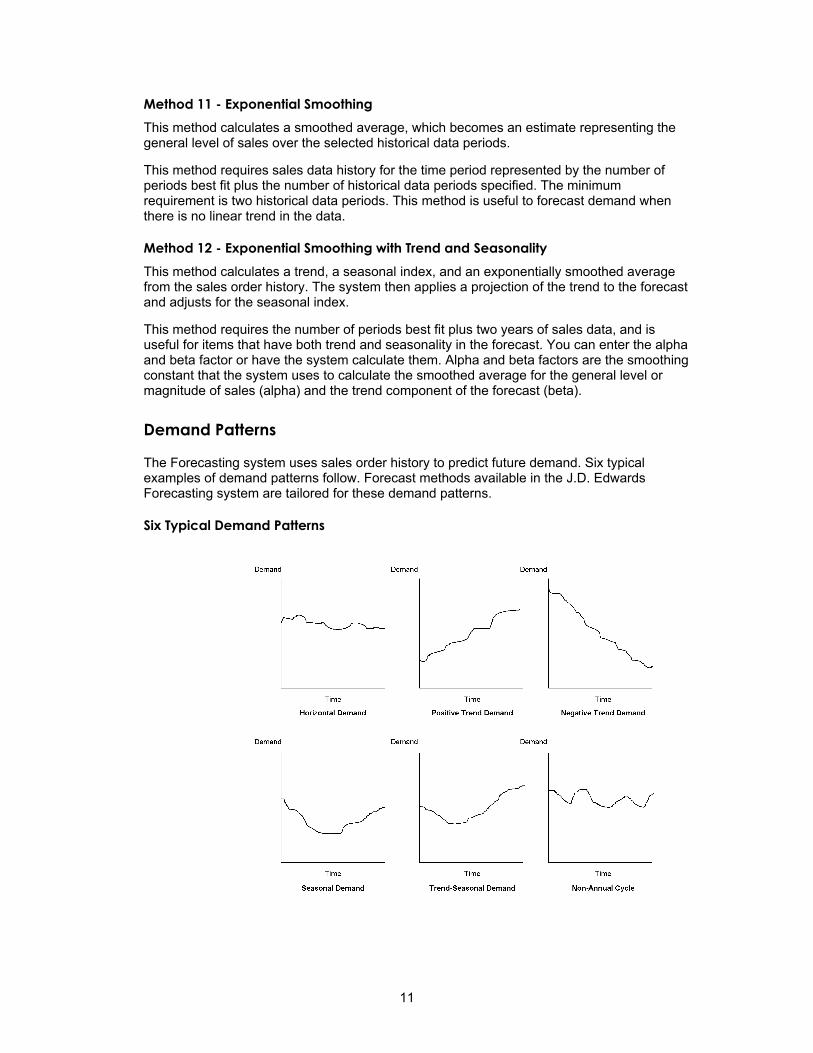
Demand Patterns
The Forecasting system uses sales order history to predict future demand. Six typical examples of demand patterns follow. Forecast methods available in the J.D. Edwards Forecasting system are tailored for these demand patterns.
Six Typical Demand Patterns
11
You can forecast the independent demand of the following information for which you have past data:
• Samples
• Promotional items
• Customer orders
• Service parts
• Interplant demands
You can also forecast demand for the following manufacturing strategy types using the manufacturing environments in which they are produced:
Make-to-stock
The manufacture of end items that meet the customers' demand that occurs after the product is completed.
Assemble-to-order
The manufacture of subassemblies that meet customers' option selections.
Make-to-order
The manufacture of raw materials and components that are stocked in order to reduce leadtime.
Forecast Accuracy
The following statistical laws govern forecast accuracy:
• A long-term forecast is less accurate than a short-term forecast because the further into the future you project the forecast, the more variables can impact the forecast.
• A forecast for a product family tends to be more accurate than a forecast for individual members of the product family. Some errors cancel each other as the forecasts for individual items summarize into the group, creating a more accurate forecast.
See Also Forecast Calculation Methods for more detail and samples of each method
Forecast Considerations
You should not rely exclusively on past data to forecast future demands. The following circumstances might affect your business and require you to review and modify your forecast:
• New products that have no past data
• Plans for future sales promotion
• Changes in national and international politics
• New laws and government regulations
• Weather changes and natural disasters
12
• Innovations from competition
• Economic changes
You can also use the following kinds of long-term trend analysis to influence the design of your forecasts:
• Market surveys
• Leading economic indicators
Forecasting Process
You extract sales order history to copy data from the Sales Order History File table (F42119), the Sales Order Detail File table (F4211), or both, into either the Forecast File table (F3460) or the Forecast Summary File table (F3400), depending on the kind of forecast you plan to generate.
You can generate detail forecasts or summaries of detail forecasts, based on data in the Forecast File table. Data from your forecasts can then be revised.
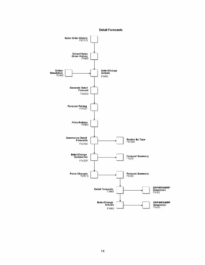
The following graphic illustrates the sequences you follow when you use the detail forecasting programs.
13
14
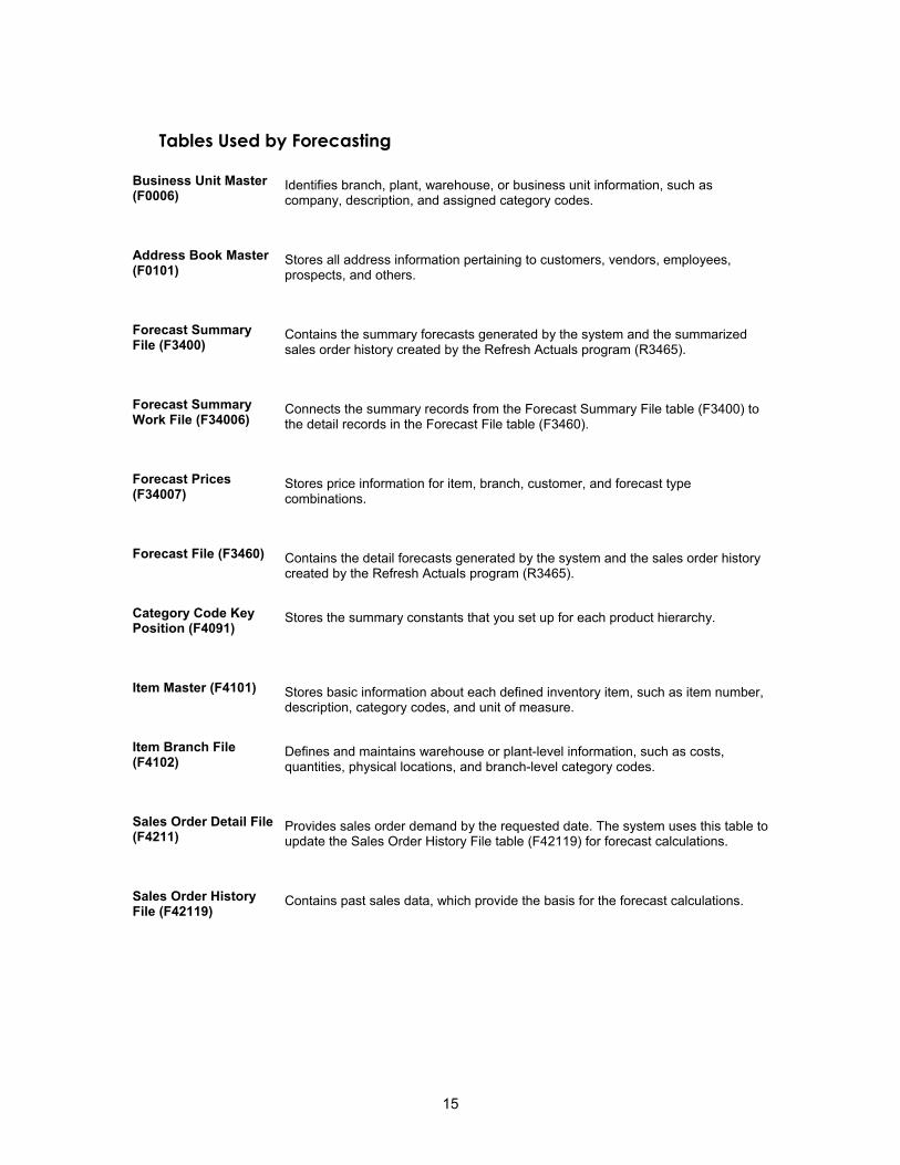
Tables Used by Forecasting
Business Unit Master (F0006)
Identifies branch, plant, warehouse, or business unit information, such as company, description, and assigned category codes.
Address Book Master (F0101)
Stores all address information pertaining to customers, vendors, employees, prospects, and others.
Forecast Summary File (F3400)
Contains the summary forecasts generated by the system and the summarized sales order history created by the Refresh Actuals program (R3465).
Forecast Summary Work File (F34006)
Connects the summary records from the Forecast Summary File table (F3400) to the detail records in the Forecast File table (F3460).
Forecast Prices (F34007)
Stores price information for item, branch, customer, and forecast type combinations.
Forecast File (F3460)
Contains the detail forecasts generated by the system and the sales order history created by the Refresh Actuals program (R3465).
Category Code Key Position (F4091)
Stores the summary constants that you set up for each product hierarchy.
Item Master (F4101)
Stores basic information about each defined inventory item, such as item number, description, category codes, and unit of measure.
Item Branch File (F4102)
Defines and maintains warehouse or plant-level information, such as costs, quantities, physical locations, and branch-level category codes.
Sales Order Detail File (F4211)
Provides sales order demand by the requested date. The system uses this table to update the Sales Order History File table (F42119) for forecast calculations.
Sales Order History File (F42119)
Contains past sales data, which provide the basis for the forecast calculations.
15
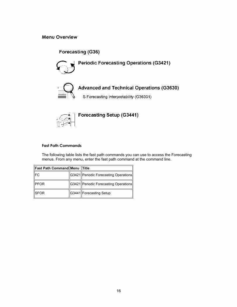
Menu Overview
Fast Path Commands
The following table lists the fast path commands you can use to access the Forecasting menus. From any menu, enter the fast path command at the command line.
Fast Path Command Menu Title
FC G3421 Periodic Forecasting Operations
PFOR G3421 Periodic Forecasting Operations
SFOR G3441 Forecasting Setup
16
Detail Forecasts
Detail forecasts are based on individual items. Use detail forecasts to project demand at the single-item level according to each item's individual history.
Forecasts are based on sales data from the Sales Order History File table (F42119) and the Sales Order Detail File table (F4211). Before you generate forecasts, you use the Extract Sales Order History program to copy sales order history information from the F42119 table and the F4211 table into the Forecast File table (F3460). This table also stores the generated forecasts.
Setting Up Detail Forecasts
Before you generate a detail forecast, you set up criteria for the dates and kinds of data on which the forecasts are based, and set up the time periods the system should use to structure the forecast output.
To set up detail forecasts, you must:
• Set up inclusion rules to specify the sales history records and current sales orders on which you want to base the forecast
• Specify beginning and ending dates for the forecast
• Indicate the date pattern on which you want to base the forecast
• Add any forecast types not already provided by the system
Topics Set up forecasting supply and demand inclusion rules
Set up forecasting fiscal date patterns
Set up the 52-period date pattern (optional)
Set up forecast types
Define large customers
Setting Up Forecasting Supply and Demand Inclusion Rules
The Forecasting system uses supply and demand inclusion rules to determine which records from the Sales Order History table (F42119) and Sales Order Detail table (F4211) to include or exclude when you run the Extract Sales Order History program. Supply and demand inclusion rules allow you to specify the status and type of items and documents to include in the records. You can set up as many different inclusion rule versions as you need for forecasting.
To forecast by weeks, set up a 52-period calendar.
17
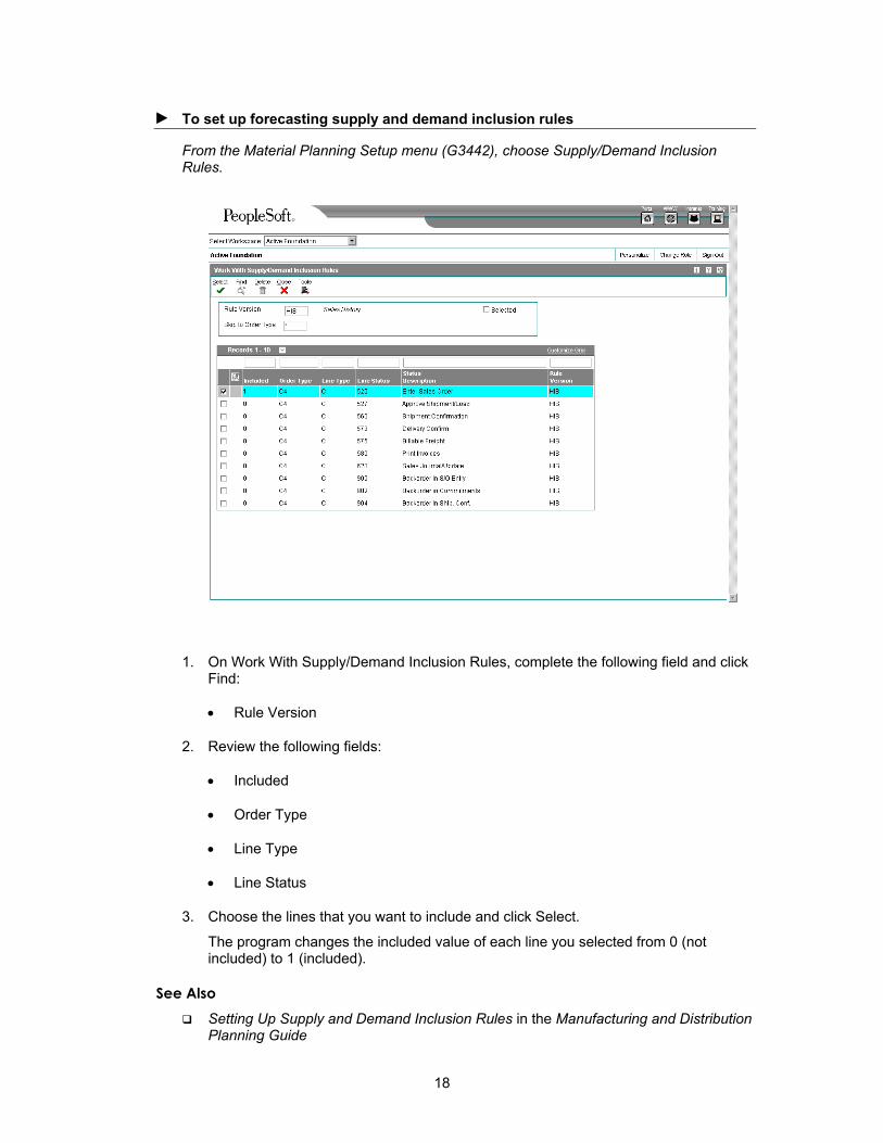
► To set up forecasting supply and demand inclusion rules
From the Material Planning Setup menu (G3442), choose Supply/Demand Inclusion Rules.
1. On Work With Supply/Demand Inclusion Rules, complete the following field and click Find:
• Rule Version
2. Review the following fields:
• Included
• Order Type
• Line Type
• Line Status
3. Choose the lines that you want to include and click Select.
The program changes the included value of each line you selected from 0 (not included) to 1 (included).
See Also Setting Up Supply and Demand Inclusion Rules in the Manufacturing and Distribution
Planning Guide
18
Setting Up Forecasting Fiscal Date Patterns
Fiscal date patterns are user defined codes (H00/DP) that identify the year and the order of the months of that year for which the system creates the forecast. The Forecasting system uses fiscal date patterns to determine the time periods into which the sales order history is grouped. Before you can generate a detail forecast, you must set up a standard monthly date pattern. The system divides the sales history into weeks or months, depending on the processing option you choose. If you want to forecast by months, you must set up the fiscal date pattern. If you want to forecast by weeks, you must set up both the fiscal date pattern and a 52-period date pattern.
To set up fiscal date patterns, specify the beginning fiscal year, current fiscal period, and which date pattern to follow. The Forecasting system uses this information during data entry, updating, and reporting. Set up fiscal date patterns for as far back as your sales history extends, and as far forward as you want to forecast.
Use the same fiscal date pattern for all forecasted items. A mix of date patterns across items that will be summarized at higher levels in the hierarchy causes unpredictable results. The fiscal date pattern must be an annual calendar, for example, from January 1, 1999 through December 31, 1999 or from June 1, 1999 through May 31, 2000.
J.D. Edwards recommends you set up a separate fiscal date pattern for forecasting only, so you can control the date pattern. If you use the date pattern already established in the Financials system, the financial officer controls the date pattern.
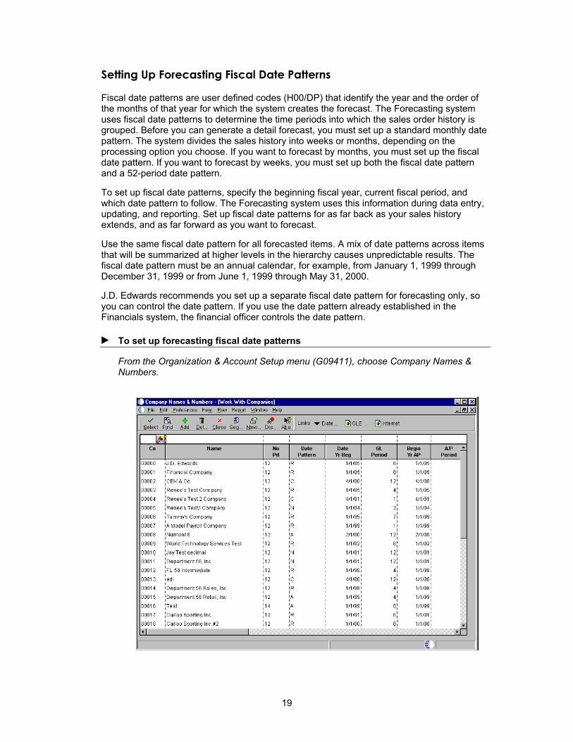
► To set up forecasting fiscal date patterns
From the Organization & Account Setup menu (G09411), choose Company Names & Numbers.
19
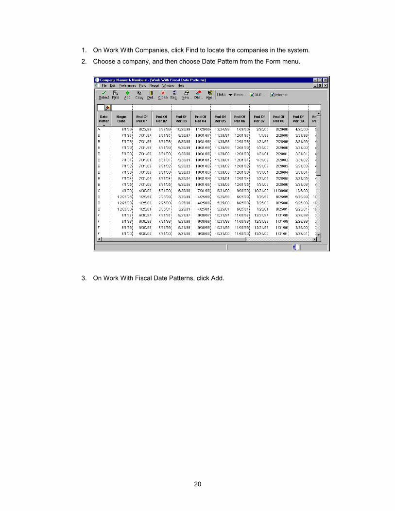
1. On Work With Companies, click Find to locate the companies in the system.
2. Choose a company, and then choose Date Pattern from the Form menu.
3. On Work With Fiscal Date Patterns, click Add.
20
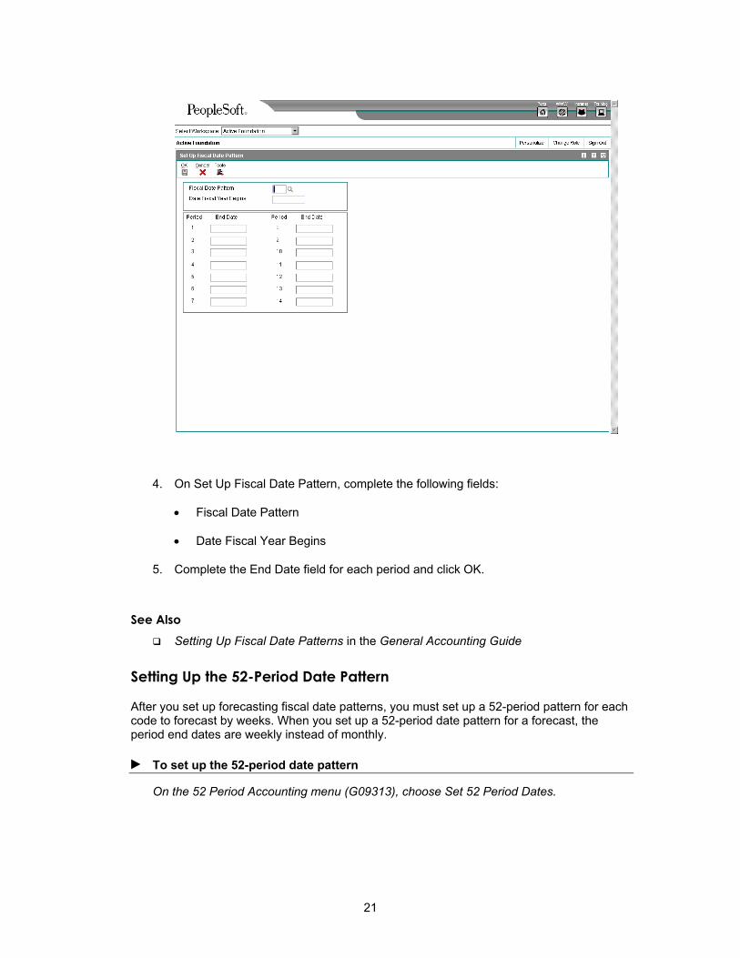
4. On Set Up Fiscal Date Pattern, complete the following fields:
• Fiscal Date Pattern
• Date Fiscal Year Begins
5. Complete the End Date field for each period and click OK.
See Also Setting Up Fiscal Date Patterns in the General Accounting Guide
Setting Up the 52-Period Date Pattern
After you set up forecasting fiscal date patterns, you must set up a 52-period pattern for each code to forecast by weeks. When you set up a 52-period date pattern for a forecast, the period end dates are weekly instead of monthly.
► To set up the 52-period date pattern
On the 52 Period Accounting menu (G09313), choose Set 52 Period Dates.
21
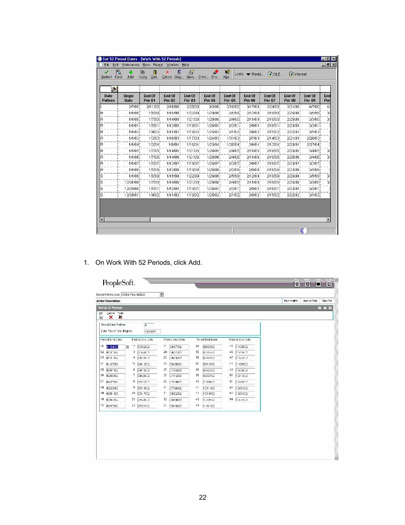
1. On Work With 52 Periods, click Add.
22
2. On Set Up 52 Periods, complete the following fields:
• Fiscal Date Pattern
• Date Fiscal Year Begins
• Date Pattern Type
3. Complete the following field for each period and click OK:
• Period End Date
Setting Up Forecast Types
You can add codes to the user defined code table (34/DF) to identify forecast types, such as BF for Best Fit and AA for sales order history. The Forecasting system uses these codes to determine which forecasting types to use when calculating a forecast. For example, using different forecast types, you can set up multiple forecasts for the same item, branch/plant, and date.
Processing options in Distribution Requirements Planning (DRP), Master Production Schedule (MPS), and Material Requirements Planning (MRP) allow you to enter forecast type codes to define which forecasting types to use in calculations. You can also use forecast type codes when you generate forecasts manually.
Defining Large Customers
For customers with significant sales demand or more activity, you can create separate forecasts and actual history records. Use this task to specify customers as large so that you can generate forecasts and actual history records for only those customers.
After you set up the customer, set the appropriate processing option so that the system searches the sales history table for sales to that customer and creates separate Detail Forecast records for them.
Use a processing option to enable the system to process larger customers by Ship To instead of Sold To.
If you included customer level in the hierarchy, the system summarizes the sales actuals with customers into separate branches of the hierarchy.
23
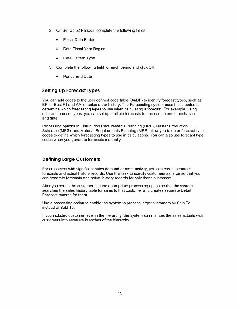
► To define large customers
From the Sales Order Management Setup menu (G4241), choose Customer Billing Instructions.
1. On Work With Customer Master, complete the following fields and click Find:
• Alpha Name
• Search Type
2. Choose the row you want to define as a large customer and click Select.
24
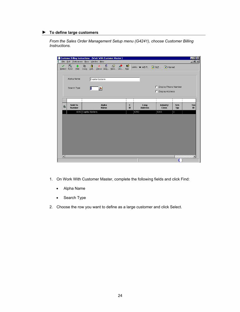
3. On Customer Master Revision, click the Credit tab, type A in the following field, and then click OK:
• ABC Code Sales
Note The ABC code indicates an item’s ABC ranking by sales amount. During ABC analysis, the system groups items by sales amount in descending order. It divides this array into three classes called A, B, and C. The A group usually represents 10% to 20% of your total items and 50% to 70% of you projected sales volume. The next grouping, B, usually represents about 20% of the items and 20% of the sales volume. The C class contains 60% to 70% of the items and represents about 10% to 30% of the sales volume. The ABC principle states that you can save effort and money when you apply different controls to the low-value, high-volume class than you apply to improve control of high-value items.
You can override a system-assigned ABC code on the Branch/Plant Item Information screen (A41026).
See Also User Defined Codes in the OneWorld Foundation Guide for detailed information
about user defined codes
25
Working with Sales Order History
The system generates detail forecasts based on sales history data, current sales data, or both, that you copy from the Sales Order History table (F42119) and the Sales Order Detail table (F4211) into the Forecast table (F3460). If you want the forecast to include current sales data, you must specify so in a processing option for the extraction program. When you copy the sales history, you specify a date range based on the request date of the sales order. The demand history data can be distorted, however, by unusually large or small values (spikes or outliers), data entry errors, or lost sales (sales orders that were cancelled due to lack of inventory).
You should review the data in the date range you specified to identify missing or inaccurate information. Then, you can revise the sales order history to account for inconsistencies and distortions before you generate the forecast.
Topics Copying sales order history
Revising sales order history
Copying Sales Order History
From the Periodic Forecasting Operations menu (G3421), choose Extract Sales Actuals.
The system generates detail and summary forecasts based on data in the Forecast table, Forecast Summary table, or both. Use Extract Sales Order History to copy the sales order history (type AA) from the Sales Order History table to the Forecast table, Forecast Summary table, or both, based upon criteria that you specify.
This program lets you:
• Select a date range for the sales order history, current sales order information, or both
• Select a version of the inclusion rules to determine which sales history to include
• Generate monthly or weekly sales order histories
• Generate a separate sales order history for a large customer
• Generate summaries
• Generate records with amounts, quantities, or both
You do not need to clear the Forecast table before you run this program. The system automatically deletes any records for the same:
• Period as the actual sales order histories to be generated
• Items
• Sales order history type
• Branch/plant
Before You Begin Set up the detail forecast generation program. See Setting Up Detail Forecasts.
Update sales order history. See Updating Customer Sales in the Sales Order Management Guide.
26
Processing Options for Refresh Actuals (R3465)
Process Tab These processing options let you specify how the system performs the following edits when generating sales history:
• Use the default forecast type
• Use the version of the Supply and Demand Inclusion Rules program (P34004)
• Use weekly or monthly planning
• Create summary records
• Use Ship To address
• Use quantities and amounts
• Include sales order detail
1. Forecast Type
Blank = AA
Use this processing option to specify the forecast type that the system uses
when creating the forecast actuals. Forecast type is a user defined code
(34/DF) that identifies the type of forecast to process. Enter the forecast
type to use as the default value or choose it from the Select User Define Code
form. If you leave this field blank, the system creates actuals from AA
forecast types.
2. Supply Demand Inclusion Rules
Use this processing option to specify the version of the Supply/Demand Inclusion Rules program (P34004) that the system uses when extracting sales
actuals. You must enter a version in this field before you can run the Extract
Sales Order History program (R3465).
Versions control how the Supply/Demand Inclusion Rules program displays
information. Therefore, you might need to set the processing options to
specific versions to meet your needs.
27
3. Actuals Consolidation
1 = Weekly
Blank = Monthly
Use this processing option to specify whether the system uses weekly or
monthly planning when creating actuals. Valid values are:
1 The system uses weekly planning.
Blank The system uses monthly planning.
4. Large Customer Summary
1 = Create
Blank = Do not create
Use this processing option to specify whether the system creates summary
records for large customers when creating actuals. Valid values are:
1 The system creates summary records for large customers.
Blank The system does not create summary records.
5. Ship To or Sold To Address
1 = Ship To
Blank = Sold To
Use this processing option to specify whether the system uses the Ship To
address on which to base large customer summaries, or the Sold To address,
when creating actuals. Valid values are:
1 The system uses the Ship To address.
Blank The system uses the Sold To address.
6. Amount or Quantity
1 = Quantity
28
2 = Amount
Blank = Both
Use this processing option to specify whether the system creates detail
forecasts with quantities, amounts, or both. Valid values are:
1 The system creates forecasts with only quantities.
2 The system creates forecasts with only amounts.
Blank The system creates forecasts with both quantities and amounts.
7. Use Active Sales Orders
1 = Active Sales Order
Blank = Sales Order History
Use this processing option to specify whether the system uses both the Sales
Order Detail table (F4211) and the Sales Order History table (F42119) when
creating actuals, or uses only the history table. Valid values are:
1 The system uses both tables.
Blank The system uses only the history table.
Dates Tab These processing options let you specify the fiscal date pattern that the system uses, and the beginning and ending dates of the records that the system includes in the processing.
1. Fiscal Date Pattern
Use this processing option to specify the fiscal date pattern that the system
uses when creating actuals. Fiscal date pattern is a user defined code
(H00/DP) that identifies the fiscal date pattern. Enter a pattern to use as
the default value or choose it from the Select User Defined Code form.
29
2. Begin Extract Date
Blank = Today's Date
Use this processing option to specify the beginning date from which the system
processes records. Enter the beginning date to use as the default value or
choose it from the Calendar. If you leave this field blank, the system uses
the system date.
3. End Extract Date
Use this processing option to specify the ending date that the system uses
when creating actuals. Enter the ending date to use as the default value or
choose it from the Calendar. Enter an ending date only if you want to include
a specific time period.
Summary Tab These processing options let you specify how the system processes the following edits:
• Create summarized forecast records
• Use summary codes
• Retrieve address book category codes
1. Summary or Detail
1 = Summary and Detail
2 = Summary only
Blank = Detail only
Use this processing option to specify whether the system creates summarized
forecast records, detail forecast records, or both. Valid values are:
1 The system creates both summarized and detail forecast records.
2 The system creates only summarized forecast records.
Blank The system creates only detail forecast records.
30
2. Forecast Summary Code
Use this processing option to specify the summary code that the system uses to
create summarized forecast records. Summary code is a user defined code
(40/KV) that identifies the code to create summarized forecast records. Enter
the code to use as the default value or choose it from the Select User Define
Code form.
3. Category Codes Address Book
1 = Sales address
Blank = Business unit
Use this processing option to specify from where the system retrieves the
address book category codes. Valid values are:
1 The system retrieves the address book number from the Forecast
table (F3460).
Blank The system uses the cost center to determine which address book
number to use to retrieve the category codes.
Interoperability Tab These processing options let you specify the default document type for the system to use for the purchase order and whether to use before or after image processing.
1. Transaction Type
Use this processing option to specify the transaction type to which the system
processes outbound interoperability transactions. Transaction type is a user
defined code (00/TT) that identifies the type of transaction. Enter a type to
use as the default value or choose it from the Select User Define Code form.
31
2. Image Processing
1 = Before Image
2 = After Image
Use this processing option to specify whether the system writes before or
after image processing. Valid values are:
1 The system writes before the images for the outbound change
transaction are processed.
Blank The system writes after the images are processed.
Revising Sales Order History
After you copy the sales order history into the Forecast table, you should review the data for spikes, outliers, entry errors, or missing demand that might distort the forecast. You can then revise the sales order history manually to account for these inconsistencies before you generate the forecast.
Enter/Change Actuals allows you to create, change, or delete a sales order history manually. You can:
• Review all entries in the Forecast table
• Revise the sales order history
• Remove invalid sales history data, such as outliers or missing demand
• Enter descriptive text for the sales order history, such as special sale or promotion information
Example: Revising Sales Order History
In this example, you run Extract Sales Order History. The program identifies the actual quantities as shown in the following form.
32
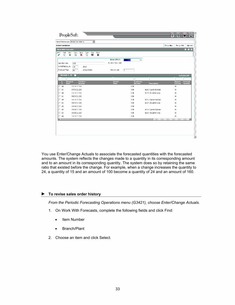
You use Enter/Change Actuals to associate the forecasted quantities with the forecasted amounts. The system reflects the changes made to a quantity in its corresponding amount and to an amount in its corresponding quantity. The system does so by retaining the same ratio that existed before the change. For example, when a change increases the quantity to 24, a quantity of 15 and an amount of 100 become a quantity of 24 and an amount of 160.
► To revise sales order history
From the Periodic Forecasting Operations menu (G3421), choose Enter/Change Actuals.
1. On Work With Forecasts, complete the following fields and click Find:
• Item Number
• Branch/Plant
2. Choose an item and click Select.
33
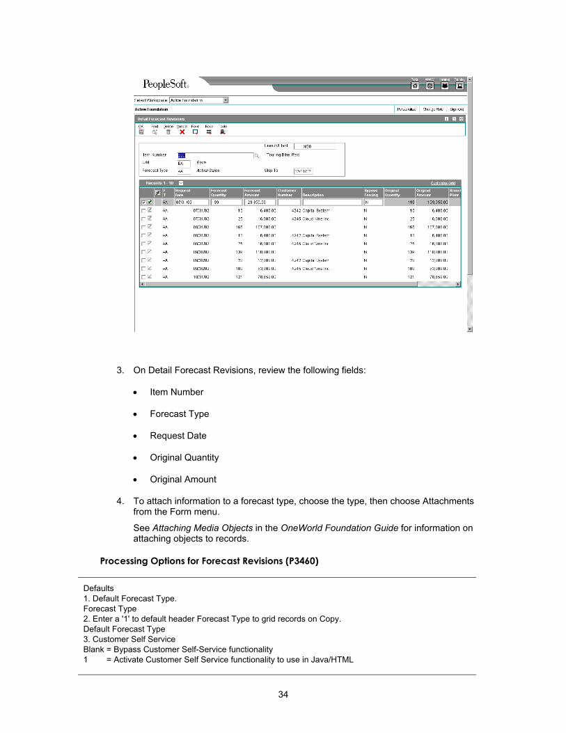
3. On Detail Forecast Revisions, review the following fields:
• Item Number
• Forecast Type
• Request Date
• Original Quantity
• Original Amount
4. To attach information to a forecast type, choose the type, then choose Attachments from the Form menu.
See Attaching Media Objects in the OneWorld Foundation Guide for information on attaching objects to records.
Processing Options for Forecast Revisions (P3460)
Defaults 1. Default Forecast Type. Forecast Type 2. Enter a '1' to default header Forecast Type to grid records on Copy. Default Forecast Type 3. Customer Self Service Blank = Bypass Customer Self-Service functionality 1 = Activate Customer Self Service functionality to use in Java/HTML
34
Interop 1. Enter the Transaction Type for processing outbound interoperability transactions Type - Transaction 2. Enter a '1' to write before images for outbound change transactions. If left blank, only after images will be written. Before Image Processing Versions Enter the version for each program. If left blank, version ZJDE0001 will be used. 1. Forecast Online Simulation (P3461) 2. Forecast Price (P34007)
Working with Detail Forecasts
After you set up the actual sales history on which you plan to base your forecast, you can generate the detail forecast. You can then revise the forecast to account for any market trends or strategies that might make future demand deviate significantly from the actual sales history.
Topics Creating detail forecasts
Reviewing detail forecasts
Revising detail forecasts
Revising forecast prices
Generating a forecast price rollup
Creating Detail Forecasts
The system creates detail forecasts by applying multiple forecasting methods to past sales histories and generating a forecast based on the method that provides the most accurate prediction of future demand. The system can also calculate a forecast based on a method that you select.
When you generate a forecast for any method, including best fit, the system rounds off the forecast amounts and quantities to the nearest whole number.
When you create detail forecasts, the system:
• Extracts sales order history information from the Forecast File table (F3460)
• Calculates the forecasts using methods that you select
• Calculates the percent of accuracy or the mean absolute deviation for each selected forecast method
• Creates a simulated forecast for the months you indicate in the processing option
• Recommends the best fit forecast method
• Creates the detail forecast in either dollars or units from the best fit forecast
The system designates the extracted actual records as type AA and the best fit model as BF. These forecast type codes are not hard-coded, so you can specify your own codes. The system stores both types of records in the Forecast table.
35
When creating detail forecasts the system allows you to:
• Specify the number of months of actual data to use to create the best fit
• Forecast for individual large customers for all methods
• Run the forecast in proof or final mode
• Forecast up to five years into the future
• Create zero forecasts, negative forecasts, or both
• Run the forecast simulation interactively
Topics Create forecasts for multiple items
Create forecasts for a single item
Creating Forecasts for Multiple Items
From the Periodic Forecasting Operations menu (G3421), choose Create Detail Forecast.
Use the Create Detail Forecast program to create detail forecasts for multiple items. Review the processing options to select the applicable values you want the program to use.
See Also R34650, Create Detail Forecast in the Reports Guide for a report sample
Processing Options for Forecast Generation (R34650)
Methods 1 - 3 Tab These processing options specify which forecast types the system uses when calculating the best fit forecast. You can also specify whether the system creates detail forecasts for the selected forecast method.
Enter 1 to use the forecast method when calculating the best fit. The system does not create detail forecasts for the method. If you enter zero before the forecast method, for example 01 for Method 1 - Percent Over Last Year, the system uses the forecast method when calculating the best fit and creates the forecast method in the Forecast File table (F3460). If you leave the field blank, the system does not use the forecast method when calculating the best fit and does not create detail forecasts for the method.
A period is defined as a week or month, depending on the pattern selected from the Date Fiscal Patterns table (F0008). For weekly forecasts, verify that you have established 52 period dates.
1. Percent Over Last Year
Blank = Do Not Use This Method
1 = Consider for Best Fit
01 = Create Detail Forecasts
36
Use this processing option to specify which type of forecast to run. This
forecast method uses the Percent Over Last Year formula to multiply each
forecast period by a percentage increase or decrease that you specify in a
processing option. This method requires the periods for the best fit plus one
year of sales history. This method is useful for seasonal items with growth or
decline. Valid values are:
Blank The system does not use this method.
1 The system calculates the best fit forecast.
01 The system uses the Percent Over Last Year formula to create detail
forecasts.
2. Percent
Any Percent Amount
Cannot be a Negative Amount
Use this processing option to specify the percent of increase or decrease used
to multiply by the sales history from last year. For example, type 110 for a
10% increase or type 97 for a 3% decrease. Valid values are any percent
amount, however, the amount cannot be a negative amount. Enter an amount to
use or choose it from the Calculator.
3. Calculated Percent Over Last Year
Blank = Do Not Use This Method
1 = Consider for Best Fit
02 = Create Detail Forecasts
Use this processing option to specify which type to run. This forecast method
37
uses the Calculated Percent Over Last Year formula to compare the periods
specified of past sales to the same periods of past sales of the previous
year. The system determines a percentage increase or decrease, then multiplies
each period by the percentage to determine the forecast. This method requires
the periods of sales order history indicated in the processing option plus one
year of sales history. This method is useful for short-term demand forecasts
of seasonal items with growth or decline. Valid values are:
Blank The system does not use this method.
1 The system calculates the best fit forecast.
02 The system uses the Calculated Percent Over Last Year formula to
create detail forecasts.
4. Number of Periods
Use this processing option to specify the number of periods to include when
calculating the percentage increase or decrease. Enter a number to use or
choose a number from the Calculator.
5. Last Year to This Year
Blank = Do Not Use This Method
1 = Consider for Best Fit
03 = Create Detail Forecasts
Use this processing option to specify which type of forecast to run. This
forecast method uses Last Year to This Year formula which uses last year's
sales for the following year's forecast. This method uses the periods best fit
plus one year of sales order history. This method is useful for mature
products with level demand or seasonal demand without a trend. Valid values
are:
38
Blank The system does not use this method.
1 The system calculates the best fit forecast.
03 The system uses the Last Year to This Year formula to create detail
forecasts.
Methods 4 - 6 Tab These processing options specify which forecast types the system uses when calculating the best fit. You can also specify whether the system creates detail forecasts for the selected forecast method.
Enter 1 to use the forecast method when calculating the best fit. The system does not create detail forecasts for the method. If you enter zero before the forecast method, for example 01 for Method 1 - Percent Over Last Year, the system uses the forecast method when calculating the best fit and creates the forecast method in the Forecast File table (F3460). If you leave the field blank, the system does not use the forecast method when calculating the best fit and does not create detail forecasts for the method.
A period is defined as a week or month, depending on the pattern selected from the Date Fiscal Patterns table (F0008). For weekly forecasts, verify that you have established 52 period dates.
1. Moving Average Blank = Do Not Use This Method 1 = Consider for Best Fit 04 = Create Detail Forecasts Use this processing option to specify which type of forecast to run. This
forecast method uses the Moving Average formula to average the months that you
indicate in the processing option to project the next period. This method uses
the periods best fit from the processing option plus the number of periods of
sales order history from the processing option. You should have the system
recalculate this forecast monthly or at least quarterly to reflect changing
demand level. This method is useful for mature products without a trend. Valid
values are:
Blank The system does not use this method.
1 The system calculates the best fit forecast.
04 The system uses the Moving Average formula to create detail
forecasts.
39
2. Number of Periods Use this processing option to specify the number of periods to include in the
average. Enter a number to use or choose a number from the Calculator.
3. Linear Approximation Blank = Do Not Use This Method 1 = Consider for Best Fit 05 Create Detail Forecasts Use this processing option to specify which type of forecast to run. This
forecast method uses the Linear Approximation formula to compute a trend from
the periods of sales order history indicated in the processing options and
projects this trend to the forecast. You should have the system recalculate
the trend monthly to detect changes in trends. This method requires periods
best fit plus the number of periods that you indicate in the processing option
of sales order history. This method is useful for new products or products
with consistent positive or negative trends that are not due to seasonal
fluctuations. Valid values are:
Blank The system does not use this method.
1 The system calculates the best fit forecast.
05 The system uses the Linear Approximation formula to create detail
forecasts.
4. Number of Periods Use this processing option to specify the number of periods to include in the
linear approximation ratio. Enter the number to use or choose a number from
the Calculator.
40
5. Least Squares Regression Blank = Do Not Use This Method 1 = Consider for Best Fit 06 = Create Detail Forecasts Use this processing option to specify which type of forecast to run. This
forecast method derives an equation describing a straight-line relationship
between the historical sales data and the passage of time. Least Squares
Regression (LSR) fits a line to the selected range of data such that the sum
of the squares of the differences between the actual sales data points and the
regression line are minimized. The forecast is a projection of this straight
line into the future. This method is useful when there is a linear trend in
the data. This method requires sales data history for the period represented
by the number of periods best fit plus the number of historical data periods
specified in the processing options. The minimum requirement is two historical
data points. Valid values are:
Blank The system does not use this method.
1 The system calculates the best fit forecast.
06 The system uses the Least Squares Regression formula to create
detail forecasts.
6. Number of Periods Use this processing option to specify the number of periods to include in the
regression. Enter the number to use or choose a number from the Calculator.
Methods 7 - 8 Tab These processing options let you specify which forecast types the system uses when calculating the best fit. You can also specify whether the system creates detail forecasts for the selected forecast method.
Enter 1 to use the forecast method when calculating the best fit. The system does not create detail forecasts for the method. If you enter zero before the forecast method, for example 01 for Method 1 - Percent Over Last Year, the system uses the forecast method when calculating the best fit and creates the forecast method in the Forecast table (F3460). If you
41
leave the field blank, the system does not use the forecast method when calculating the best fit and does not create detail forecasts for the method.
A period is defined as a week or month, depending on the pattern selected from the Date Fiscal Patterns table (F0008). For weekly forecasts, verify that you have established 52 period dates.
1. Second Degree Approximation
Blank = Do Not Use This Method
1 = Consider for Best Fit
07 = Create Detail Forecasts
Use this processing option to specify which type of forecast to run. This
method uses the Second Degree Approximation formula to plot a curve based on
the number of periods of sales history indicated in the processing options to
project the forecast. This method adds the periods best fit and the number of
periods, and then multiplies by three. You indicate the number of periods in
the processing option of sales order history. This method is not useful for
long-term forecasts. Valid values are:
Blank The system does not use this method.
1 The system calculates the best fit forecast.
07 The system uses the Second Degree Approximation formula to create
detail forecasts.
2. Number of Periods
Use this processing option to specify the number of periods to include in the
approximation. Enter the number to use or choose a number from the Calculator.
3. Flexible Method
Blank = Do Not Use This Method
1 = Consider For Best Fit
42
08 = Create Detail
Use this processing option to specify which type of forecast to run. This
forecast method specifies the periods best fit block of sales order history
starting "n" months prior and a percentage increase or decrease with which to
modify it. This method is similar to Method 1 - Percent Over Last Year, except
that you can specify the number of periods that you use as the base. Depending
on what you select as "n", this method requires periods best fit plus the
number of periods indicated in the processing options of sales data. This
method is useful for a planned trend. Valid values are:
Blank The system does not use this method.
1 The system calculates the best fit forecast.
08 The system uses the Flexible method to create detail forecasts.
4. Number of Periods
Use this processing option to specify the number of periods prior to the best
fit that you want to include in the calculation. Enter the number to use or
choose a number from the Calculator.
5. Percent Over Prior Period
Any Percent Amount
Cannot be a Negative Amount
Use this processing option to specify the percent of increase or decrease for
the system to use. For example, type 110 for a 10% increase or type 97 for a
3% decrease. You can enter any percent amount, however, the amount cannot be a
negative amount.
43
Method 9 Tab These processing options let you specify which forecast types the system uses when calculating the best fit. You can also specify whether the system creates detail forecasts for the selected forecast method.
Enter 1 to have the system use the forecast method when calculating the best fit. The system does not create detail forecasts for the method. If you enter zero before the forecast method, for example 01 for Method 1 - Percent Over Last Year, the system uses the forecast method when calculating the best fit and creates the forecast method in the Forecast table (F3460). If you leave the field blank, the system does not use the forecast method when calculating the best fit and does not create detail forecasts for the method.
The total of all the weights used in the Weighted Moving Average calculation must equal 100. If you do not enter a weight for a period within the specified number of periods, the system uses a weight of zero for that period. The system does not use weights entered for periods greater than the number of specified periods.
A period is defined as a week or month, depending on the pattern selected from the Date Fiscal Patterns table (F0008). For weekly forecasts, verify that you have established 52 period dates.
1. Weighted Moving Average
Blank = Do Not Use This Method
1 = Consider for Best Fit
09 = Create Detail Forecasts
Use this processing option to specify which type of forecast to use. The
Weighted Moving Average forecast formula is similar to Method 4 - Moving
Average formula, because it averages the previous number of months of sales
history indicated in the processing options to project the next month's sales
history. However, with this formula you can assign weights for each of the
prior periods in a processing option. This method requires the number of
weighted periods selected plus periods best fit data. Similar to Moving
Average, this method lags demand trends, so it is not recommended for products
with strong trends or seasonality. This method is useful for mature products
with demand that is relatively level. Valid values are:
Blank The system does not use this forecast.
1 The system calculates the best fit forecast.
09 The system uses the Weighted Moving Average formula to create
44
detail forecasts.
2. One Period Prior
Use this processing option to specify the weight to assign to one period prior
for calculating a moving average. Enter the number to use or choose it from
the Calculator.
3. Two Periods Prior
Use this processing option to specify the weight to assign to two periods
prior for calculating a moving average. Enter a number to use or choose it
from the Calculator.
4. Three Periods Prior
Use this processing option to specify the weight to assign to three periods
prior for calculating a moving average. Enter the number to use or choose it
from the Calculator.
5. Four Periods Prior
Use this processing option to specify the weight to assign to four periods
prior for calculating a moving average. Enter the number to use or choose it
from the Calculator.
6. Five Periods Prior
Use this processing option to specify the weight to assign to five periods
prior for calculating a moving average. Enter the number to use or choose a
number from the Calculator.
45
7. Six Periods Prior
Use this processing option to specify the weight to assign to six periods
prior for calculating a moving average. Enter the number to use or choose a
number from the Calculator.
8. Seven Periods Prior
Use this processing option to specify the weight to assign to seven periods
prior for calculating a moving average. Enter a number to use or choose a
number from the Calculator.
9. Eight Periods Prior
Use this processing option to specify the weight to assign to eight periods
prior for calculating a moving average. Enter the number to use or choose a
number from the Calculator.
10. Nine Periods Prior
Use this processing option to specify the weight to assign to nine periods
prior for calculating a moving average. Enter the number to use or choose a
number from the Calculator.
11. Ten Periods Prior
Use this processing option to specify the weight to assign to 10 periods prior
for calculating a moving average. Enter the number to use or choose a number
from the Calculator.
46
12. Eleven Periods Prior
Use this processing option to specify the weight to assign to 11 periods prior
for calculating a moving average. Enter the number to use or choose a number
from the Calculator.
13. Twelve Periods Prior
Use this processing option to specify the weight to assign to 12 periods prior
for calculating a moving average. Enter the number to use or choose a number
from the Calculator.
14. Periods to Include
Use this processing option to specify the number of periods to include. Enter
the number to use or choose a number from the Calculator.
Methods 10 - 11 Tab These processing options let you specify which forecast types the system uses when calculating the best fit. You can also specify whether the system creates detail forecasts for the selected forecast method.
Enter 1 to use the forecast method when calculating the best fit. No detail forecasts are created for the method. If you enter the method number, for example 11 for Method 11 - Exponential Smoothing, the system uses the forecast method when calculating the best fit and creates the forecast method in the Forecast table (F3460). If the field is blank, the system does not use the forecast method when calculating the best fit and no detail forecasts are created for the method
A period is defined as a week or month, depending on the pattern selected from the Date Fiscal Patterns table (F0008). For weekly forecasts, verify that you have established 52 period dates.
1. Linear Smoothing
Blank = Do Not Use This Method
47
1 = Consider for Best Fit
10 = Create Detail Forecasts
Use this processing option to specify which type of forecast to run. This
forecast method calculates a weighted average of past sales data. You can
specify the number of periods of sales order history to use in the calculation
(from 1 to 12) in a processing option. The system uses a mathematical
progression to weigh data in the range from the first (least weight) to the
final (most weight). Then, the system projects this information for each
period in the forecast. This method requires the periods best fit plus the
number of periods of sales order history from the processing option. Valid
values are:
Blank The system does not use this method.
1 The system calculates the best fit forecast.
10 The system uses the Linear Smoothing method to create detail
forecasts.
2. Number of Periods
Use this processing option to specify the number of periods to include in the
smoothing average. Enter the number to use or choose a number from the
Calculator.
3. Exponential Smoothing
Blank = Do Not Use This Method
1 = Consider for Best Fit
11 = Create Detail Forecasts
Use this processing option to specify which type of forecast to run. This
48
forecast method uses one equation to calculate a smoothed average. This
becomes an estimate representing the general level of sales over the selected
historical range. This method is useful when there is no linear trend in the
data. This method requires sales data history for the time period represented
by the number of periods best fit plus the number of historical data periods
specified in the processing options. The minimum requirement is two historical
data periods. Valid values are:
Blank The system does not use this method.
1 The system calculates the best fit forecast.
11 The system uses the Exponential Smoothing method to create detail
forecasts.
4. Number of Periods
Use this processing option to specify the number of periods to include in the
smoothing average. Enter the number to use or choose a number from the
Calculator.
5. Alpha Factor
0 - 1
Use this processing option to specify the alpha factor, a smoothing constant,
the system uses to calculate the smoothed average for the general level or
magnitude of sales. You can enter any amount, including decimals, from zero to
one.
49
Method 12 Tab These processing options let you specify which forecast types the system uses when calculating the best fit. You can also specify whether the system creates detail forecasts for the selected forecast method.
Enter 1 to use the forecast method when calculating the best fit. No detail forecasts are created for the method. If you enter the method number before the forecast method, for example 12 for Method 12 - Exponential Smoothing With Trend and Seasonality, the system uses the forecast method when calculating the best fit and creates the forecast method in the Forecast table (F3460). If the field is blank, the system does not use the forecast method when calculating the best fit and no detail forecasts are created for the method.
A period is defined as a week or month, depending on the pattern selected from the Date Fiscal Patterns table (F0008). For weekly forecasts, verify that you have established 52 period dates.
1. Exponential Smoothing with Trend and Seasonality
Blank = Do Not Use This Method
1 = Consider for Best Fit
12 = Create Detail Forecasts
Use this processing option to specify which type of forecast to run. This
forecast method calculates a trend, a seasonal index, and an exponentially
smoothed average from the sales order history. The system then applies a
projection of the trend to the forecast and adjusts for the seasonal index.
This method requires months best fit plus two years of sales data and is
useful for items that have both trend and seasonality in the forecast. Use the
processing options to enter the alpha and beta factor rather than have the
system calculate them. Valid values are:
Blank The system does not use this method.
1 The system calculates the best fit forecast.
12 The system uses the Exponential Smoothing with T&S method to create
detail forecasts.
2. Alpha Factor
50
0 - 1
Use this processing option to specify the alpha factor, a smoothing constant,
the system uses to calculate the smoothed average for the general level or
magnitude of sales. You can enter any amount, including decimals, from zero to
one.
3. Beta Factor
0 - 1
Use this processing option to specify the beta factor, a smoothing constant,
the system uses to calculate the smoothed average for the trend component of
the forecast. You can enter any amount, including decimals, from zero to one.
4. Seasonality
0 = Do Not Include Seasonality
1 = Include Seasonality
Use this processing option to specify whether the system includes seasonality
in the calculation. Valid values are:
0 The system does not include seasonality.
1 The system includes seasonality.
Blank The system does not include seasonality.
51
Defaults Tab These processing options let you specify the defaults the system uses to calculate forecasts. The system extracts actual values from Sales History and stores the forecasts that are generated in the Forecast table (F3460). You can define your own forecast types for Actuals (AA) and best fit (BF).
1. Actuals Forecast Type
Use this processing option to specify the forecast type that identifies the
sales order history used as the basis for the forecast calculations, or
Actuals. Forecast type is a user defined code (34/DF) that identifies the type
of forecast to run. Enter the forecast type to use as the default value or
choose it from the Select User Define Code form.
2. Best Fit Forecast Type
Use this processing option to specify the forecast type that is generated as a
result of the best fit calculation. Forecast type is a user defined code
(34/DF) that identifies the type of forecast to run. Enter the forecast type
to use as the default value or choose it from the Select User Define Code
form.
Process Tab These processing options let you specify whether the system:
• Runs the Forecast Generation program in proof or final mode
• Creates forecasts for large customers
• Creates weekly or monthly forecasts
In addition, you use the processing options to specify:
• The start date, length, and data used when the system creates forecasts
• How the system calculates the best fit forecast
The system applies the selected forecasting methods to past sales order history and compares the forecast simulation to the actual history. When you generate a forecast, the system compares actual sales order histories to forecasts for the months or weeks you indicate in the processing option and computes how accurately each of the selected
52
forecasting methods would have predicted sales. Then, the system recommends the most accurate forecast as the best fit.
Mean Absolute Deviation (MAD) is the mean of the absolute values of the deviations between actual and forecast data. MAD is a measure of the average magnitude of errors to expect, given a forecasting method and data history. Because absolute values are used in the calculation, positive errors do not cancel out negative errors. When comparing several forecasting methods, the one with the smallest MAD has shown to be the most reliable for that product for that holdout period.
Percent of Accuracy (POA) is a measure of forecast bias. When forecasts are consistently too high, inventories accumulate and inventory costs rise. When forecasts are consistently too low, inventories are consumed and customer service declines. A forecast that is 10 units too low, then 8 units too high, then 2 units too high, is an unbiased forecast. The positive error of 10 is canceled by negative errors of 8 and 2.
1. Mode
Blank = Proof Mode
1 = Final Mode
Use this processing option to specify whether the system runs in proof or
final mode. Valid values are:
Blank The system runs in proof mode, creating a simulation report.
1 The system runs in final mode, creating forecast records.
2. Large Customers
Blank = Do Not Create Large
Customer Forecasts
1 = Create Large Customer Forecasts
Use this processing option to specify whether to create forecasts for large
customers. Based on the Customer Master table (F0301), if the ABC code is set
to A and this option is set to 1 the system creates separate forecasts for
large customers. Valid values are:
Blank The system does not create large customer forecasts.
53
1 The system creates large customer forecasts.
3. Weekly Forecasts
Blank = Monthly Forecasts
1 = Weekly Forecasts
Use this processing option to specify weekly or monthly forecasts. For weekly
forecasts, use fiscal date patterns with 54 periods. For monthly forecasts,
use fiscal date patterns with 14 periods. Valid values are:
Blank The system creates monthly forecasts.
1 The system creates weekly forecasts.
4. Start Date
Blank = Today's date
Use this processing option to specify the date on which the system starts the
forecasts. Enter a date to use or choose a date from the Calendar. If you
leave this field blank, the system uses the system date.
5. Forecast Length
Blank = 3 periods
Use this processing option to specify the number of periods to forecast. You
must have previously established fiscal date patterns for the forecasted
periods. If you leave this field blank, the system uses 3.
6. Actual Data
54
Blank = 3 periods
Use this processing option to specify the number of periods of actual data
that the system uses to calculate the best fit forecast. If you leave this
field blank, the system uses 3.
The system applies the selected forecasting methods to past sales order
history and compares the forecast simulation to the actual history. When you
generate a forecast, the system compares actual sales order histories to
forecasts for the months or weeks you indicate in the processing option and
computes how accurately each of the selected forecasting methods would have
predicted sales. Then, the system recommends the most accurate forecast as the
best fit.
7. Mean Absolute Deviation
Blank = Percent of Accuracy
1 = Mean Absolute Deviation
Use this processing option to specify whether the system uses the Mean
Absolute Deviation formula or the Percent of Accuracy formula to calculate the
best fit forecast. Valid values are:
Blank The system uses the Percent of Accuracy formula.
1 The system uses the Mean Absolute Deviation formula.
8. Amounts or Quantity
Blank = Quantity
1 = Amount
55
Use this processing option to specify whether the system calculates the best
fit forecast using amounts or quantities. If you specify to use amounts, you
must also extract sales history using amounts. This also affects forecast
pricing. Valid values are:
Blank The system uses quantities.
1 The system uses amounts.
9. Fiscal Date Pattern
Use this processing option to specify the fiscal date pattern type to use for
the forecast calculations. When generating weekly forecasts, the fiscal date
pattern defined here must be set up for 52 periods.
10. Negative Values
Blank = Zeros
1 = Negative Values
Use this processing option to specify whether the system displays negative
values. Valid values are:
Blank The system substitutes a zero value for all negative values.
1 The system displays negative values.
56
Interoperability Tab This processing option lets you specify the transaction type the system uses for interoperability.
1. Transaction Type
Blank = Do Not Create Outbound Forecast
JDEFC = Create Outbound Forecast
Use this processing option to specify the transaction type used for
interoperability. Valid values are:
Blank The system does not create outbound forecasts.
JDEFC The system creates outbound forecasts.
Creating Forecasts for a Single Item
Use Online Simulation to create a detail forecast for a single item. After you run the simulation interactively, you can modify the simulated forecast and commit it to the Forecast File table (F3460).
See Also Forecast Calculation Methods for more information about the forecast types and how
the system calculates forecasts and best fit
57
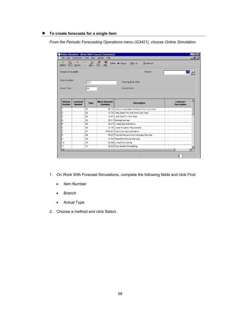
► To create forecasts for a single item
From the Periodic Forecasting Operations menu (G3421), choose Online Simulation.
1. On Work With Forecast Simulations, complete the following fields and click Find:
• Item Number
• Branch
• Actual Type
2. Choose a method and click Select.
58
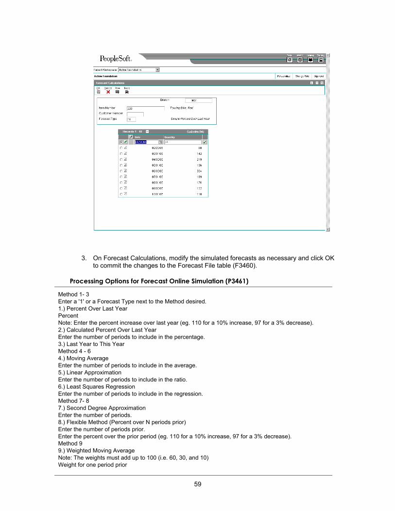
3. On Forecast Calculations, modify the simulated forecasts as necessary and click OK to commit the changes to the Forecast File table (F3460).
Processing Options for Forecast Online Simulation (P3461)
Method 1- 3 Enter a '1' or a Forecast Type next to the Method desired. 1.) Percent Over Last Year Percent Note: Enter the percent increase over last year (eg. 110 for a 10% increase, 97 for a 3% decrease). 2.) Calculated Percent Over Last Year Enter the number of periods to include in the percentage. 3.) Last Year to This Year Method 4 - 6 4.) Moving Average Enter the number of periods to include in the average. 5.) Linear Approximation Enter the number of periods to include in the ratio. 6.) Least Squares Regression Enter the number of periods to include in the regression. Method 7- 8 7.) Second Degree Approximation Enter the number of periods. 8.) Flexible Method (Percent over N periods prior) Enter the number of periods prior. Enter the percent over the prior period (eg. 110 for a 10% increase, 97 for a 3% decrease). Method 9 9.) Weighted Moving Average Note: The weights must add up to 100 (i.e. 60, 30, and 10) Weight for one period prior
59
Weight for two periods prior Weight for three periods prior Weight for four periods prior Method 9 Cont. Weight for five periods prior Weight for six periods prior Weight for seven periods prior Weight for nine periods prior Weight for nine periods prior Weight for ten periods prior Method 9 Cont. Weight for eleven periods prior Weight for twelve periods prior Note: If no weight is entered for a period within the number of periods specified, a weight of zero will be used for that period. Weights entered for periods greater than the number of periods specified will not be used. Enter the number of periods to include. Method 10-11 10.) Linear Smoothing Enter the number of periods to include in smoothing average. 11.) Exponential Smoothing Enter the number of periods to include in the smoothing average. Enter the Alpha factor. If zero it will be calculated. Method 12 12.) Exponentail Smoothing with Trend and Seasonality factors Enter the Alpha factor. If zero it will be calculated. Enter the Beta factor. If zero it will be calculated. Enter a '1' to include seasonality in the calculation. If blank seasonality will not be used. Process 1 1.) Enter the Forecast Type to use when creating the Best Fit Forecast. 2.) Enter a '1' to create summary records for large customers (ABC = type). 3.) Enter a '1' to specify weekly forecasts. Blank defaults to monthly. 4.) Enter the date to start forecasts. Default of today's date if left blank. 5.) Enter Number of periods to forecast. Default to 3 periods if blank. 6.) Enter the number of periods of actual data to be used to calculate best fit forecast. If left blank 3 periods of data will be used. Process 2 7.) Enter a '1' to calculate Best Fit forecast using Mean Absolute Deviation. Blank will calculate the Best Fit using Percent of Accuracy. 8.) Enter a '1' to forecast using amounts. Default of blank will forecast quantities. 9.) Enter the Fiscal Date Pattern Type to use for forecast dating. 10.) Enter a '1' to allow negative values to be written. If left blank, negative values will be written as zeroes. Versions Enter the version for each program. If left blank, version ZJDE0001 will be used. 1. Forecast Review by Type (P34300)
60
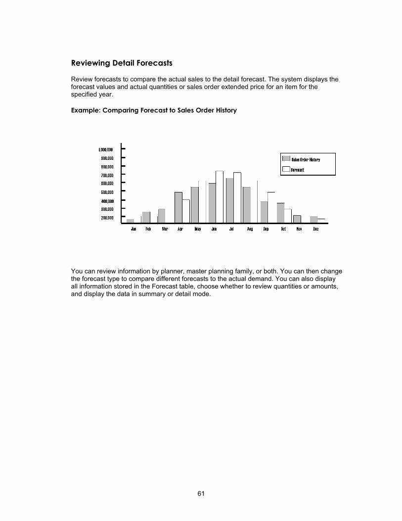
Reviewing Detail Forecasts
Review forecasts to compare the actual sales to the detail forecast. The system displays the forecast values and actual quantities or sales order extended price for an item for the specified year.
Example: Comparing Forecast to Sales Order History
You can review information by planner, master planning family, or both. You can then change the forecast type to compare different forecasts to the actual demand. You can also display all information stored in the Forecast table, choose whether to review quantities or amounts, and display the data in summary or detail mode.
61
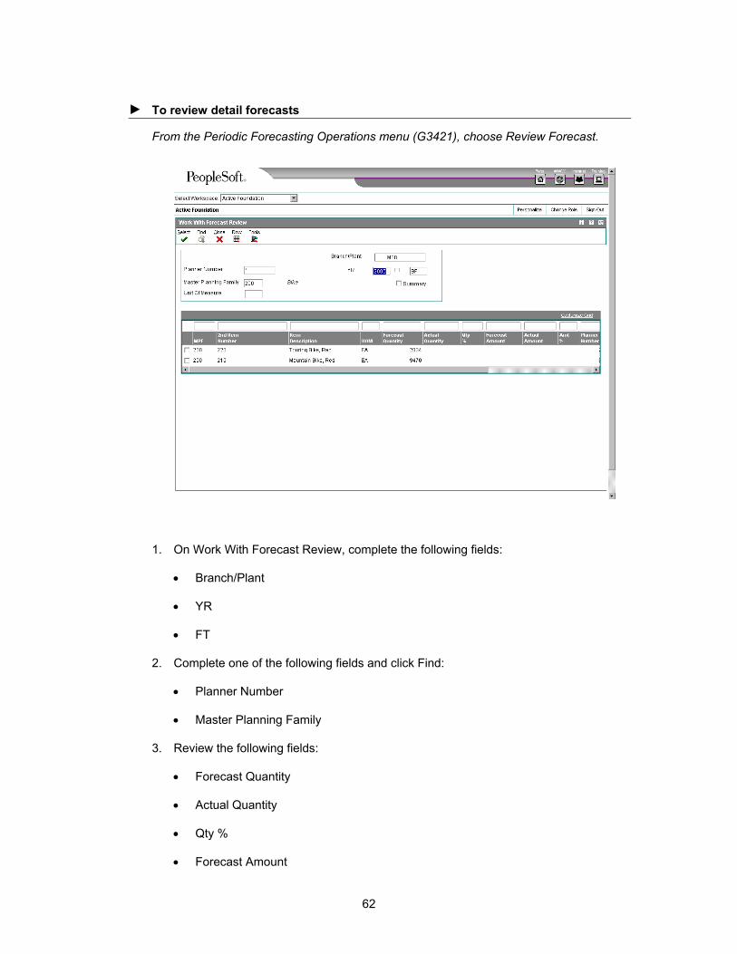
► To review detail forecasts
From the Periodic Forecasting Operations menu (G3421), choose Review Forecast.
1. On Work With Forecast Review, complete the following fields:
• Branch/Plant
• YR
• FT
2. Complete one of the following fields and click Find:
• Planner Number
• Master Planning Family
3. Review the following fields:
• Forecast Quantity
• Actual Quantity
• Qty %
• Forecast Amount
62
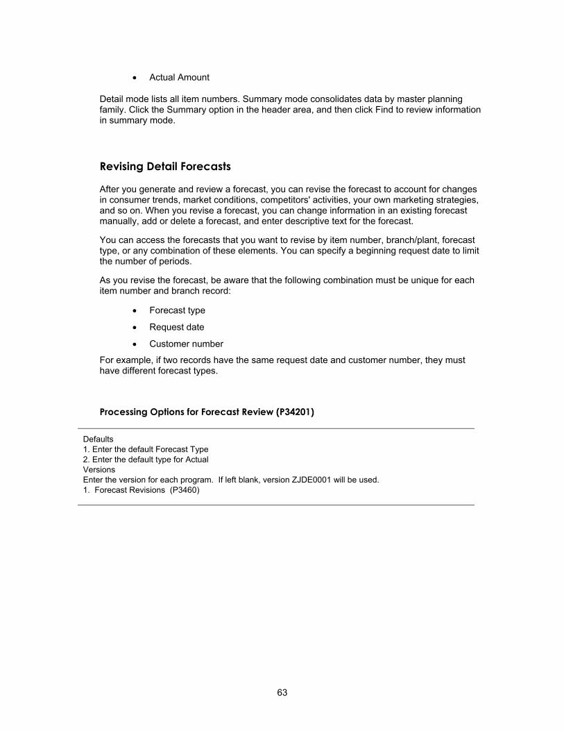
• Actual Amount
Detail mode lists all item numbers. Summary mode consolidates data by master planning family. Click the Summary option in the header area, and then click Find to review information in summary mode.
Revising Detail Forecasts
After you generate and review a forecast, you can revise the forecast to account for changes in consumer trends, market conditions, competitors' activities, your own marketing strategies, and so on. When you revise a forecast, you can change information in an existing forecast manually, add or delete a forecast, and enter descriptive text for the forecast.
You can access the forecasts that you want to revise by item number, branch/plant, forecast type, or any combination of these elements. You can specify a beginning request date to limit the number of periods.
As you revise the forecast, be aware that the following combination must be unique for each item number and branch record:
• Forecast type
• Request date
• Customer number
For example, if two records have the same request date and customer number, they must have different forecast types.
Processing Options for Forecast Review (P34201)
Defaults 1. Enter the default Forecast Type 2. Enter the default type for Actual Versions Enter the version for each program. If left blank, version ZJDE0001 will be used. 1. Forecast Revisions (P3460)
63
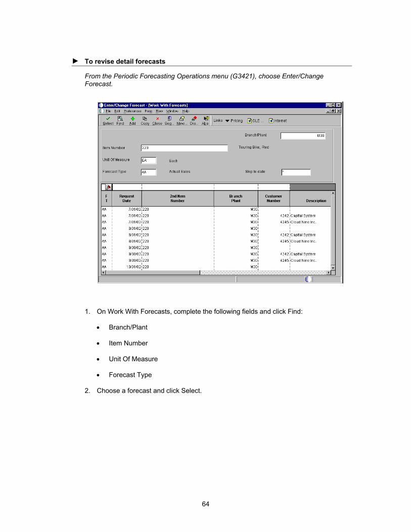
► To revise detail forecasts
From the Periodic Forecasting Operations menu (G3421), choose Enter/Change Forecast.
1. On Work With Forecasts, complete the following fields and click Find:
• Branch/Plant
• Item Number
• Unit Of Measure
• Forecast Type
2. Choose a forecast and click Select.
64
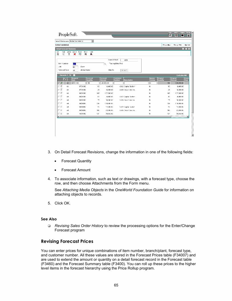
3. On Detail Forecast Revisions, change the information in one of the following fields:
• Forecast Quantity
• Forecast Amount
4. To associate information, such as text or drawings, with a forecast type, choose the row, and then choose Attachments from the Form menu.
See Attaching Media Objects in the OneWorld Foundation Guide for information on attaching objects to records.
5. Click OK.
See Also Revising Sales Order History to review the processing options for the Enter/Change
Forecast program
Revising Forecast Prices
You can enter prices for unique combinations of item number, branch/plant, forecast type, and customer number. All these values are stored in the Forecast Prices table (F34007) and are used to extend the amount or quantity on a detail forecast record in the Forecast table (F3460) and the Forecast Summary table (F3400). You can roll up these prices to the higher level items in the forecast hierarchy using the Price Rollup program.
65
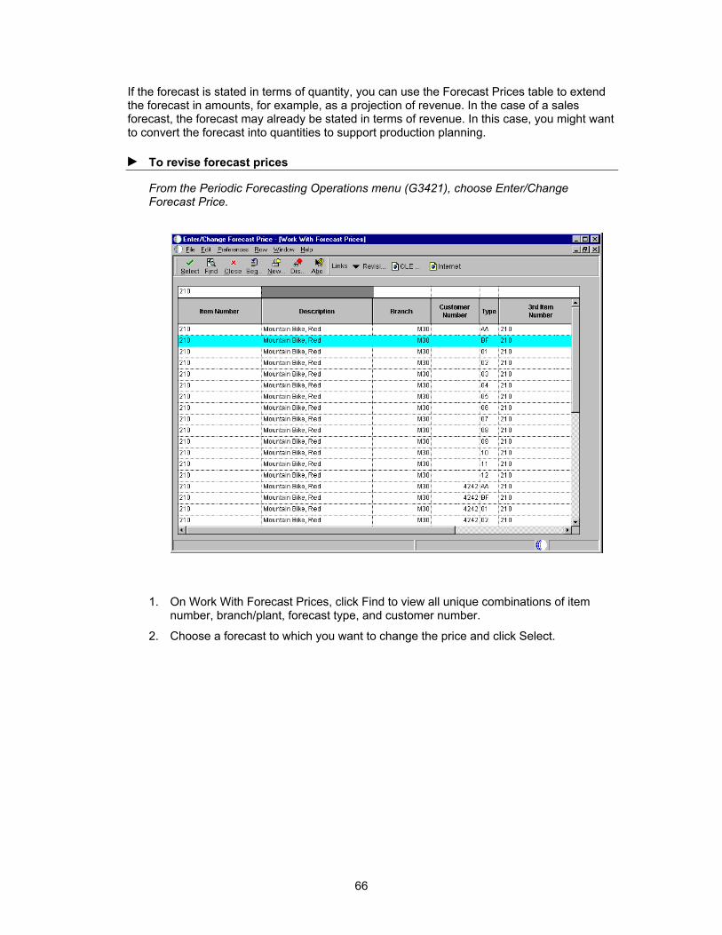
If the forecast is stated in terms of quantity, you can use the Forecast Prices table to extend the forecast in amounts, for example, as a projection of revenue. In the case of a sales forecast, the forecast may already be stated in terms of revenue. In this case, you might want to convert the forecast into quantities to support production planning.
► To revise forecast prices
From the Periodic Forecasting Operations menu (G3421), choose Enter/Change Forecast Price.
1. On Work With Forecast Prices, click Find to view all unique combinations of item number, branch/plant, forecast type, and customer number.
2. Choose a forecast to which you want to change the price and click Select.
66
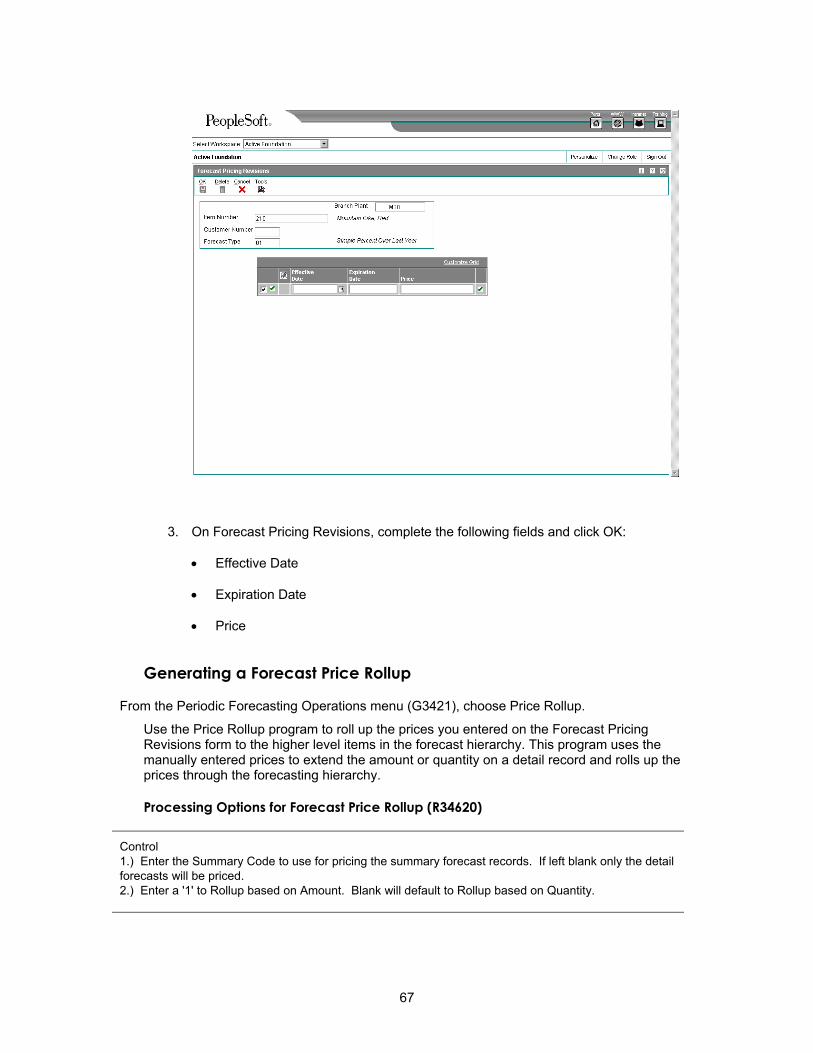
3. On Forecast Pricing Revisions, complete the following fields and click OK:
• Effective Date
• Expiration Date
• Price
Generating a Forecast Price Rollup
From the Periodic Forecasting Operations menu (G3421), choose Price Rollup.
Use the Price Rollup program to roll up the prices you entered on the Forecast Pricing Revisions form to the higher level items in the forecast hierarchy. This program uses the manually entered prices to extend the amount or quantity on a detail record and rolls up the prices through the forecasting hierarchy.
Processing Options for Forecast Price Rollup (R34620)
Control 1.) Enter the Summary Code to use for pricing the summary forecast records. If left blank only the detail forecasts will be priced. 2.) Enter a '1' to Rollup based on Amount. Blank will default to Rollup based on Quantity.
67
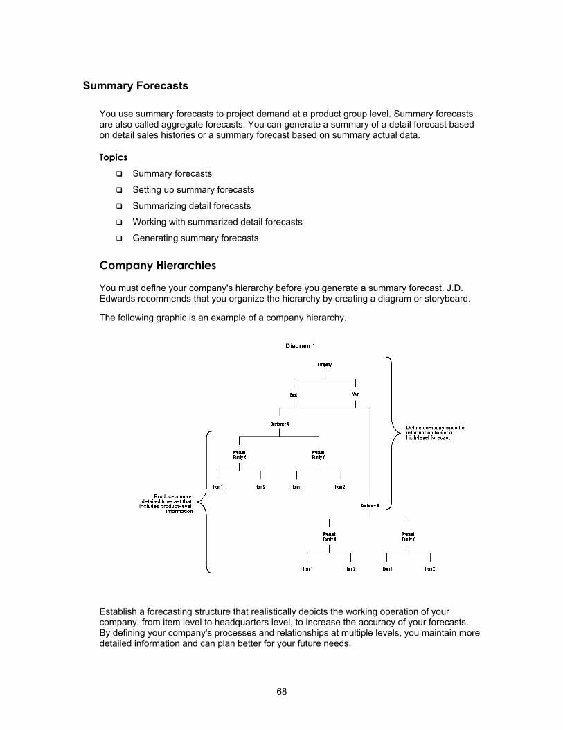
Summary Forecasts
You use summary forecasts to project demand at a product group level. Summary forecasts are also called aggregate forecasts. You can generate a summary of a detail forecast based on detail sales histories or a summary forecast based on summary actual data.
Topics Summary forecasts
Setting up summary forecasts
Summarizing detail forecasts
Working with summarized detail forecasts
Generating summary forecasts
Company Hierarchies
You must define your company's hierarchy before you generate a summary forecast. J.D. Edwards recommends that you organize the hierarchy by creating a diagram or storyboard.
The following graphic is an example of a company hierarchy.
Establish a forecasting structure that realistically depicts the working operation of your company, from item level to headquarters level, to increase the accuracy of your forecasts. By defining your company's processes and relationships at multiple levels, you maintain more detailed information and can plan better for your future needs.
68
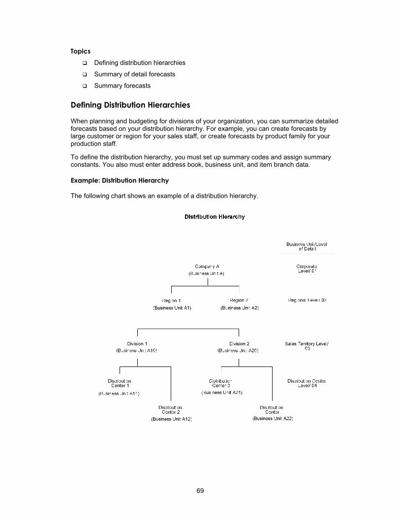
Topics Defining distribution hierarchies
Summary of detail forecasts
Summary forecasts
Defining Distribution Hierarchies
When planning and budgeting for divisions of your organization, you can summarize detailed forecasts based on your distribution hierarchy. For example, you can create forecasts by large customer or region for your sales staff, or create forecasts by product family for your production staff.
To define the distribution hierarchy, you must set up summary codes and assign summary constants. You also must enter address book, business unit, and item branch data.
Example: Distribution Hierarchy
The following chart shows an example of a distribution hierarchy.
69
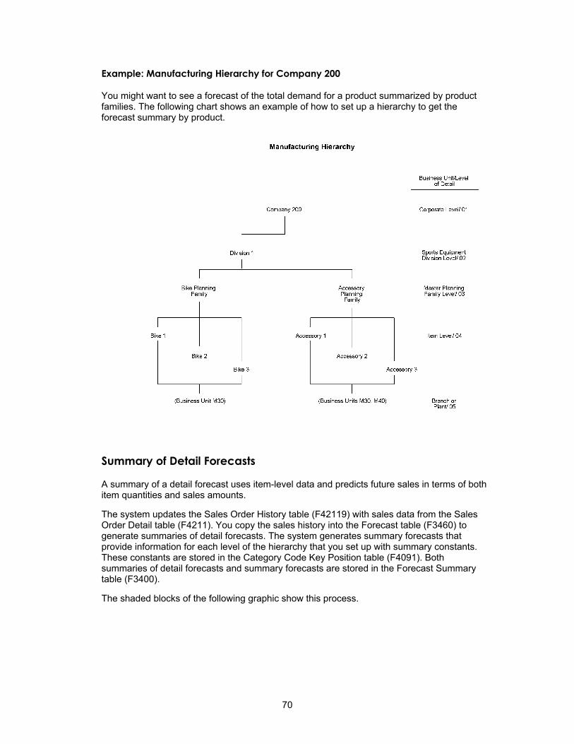
Example: Manufacturing Hierarchy for Company 200
You might want to see a forecast of the total demand for a product summarized by product families. The following chart shows an example of how to set up a hierarchy to get the forecast summary by product.
Summary of Detail Forecasts
A summary of a detail forecast uses item-level data and predicts future sales in terms of both item quantities and sales amounts.
The system updates the Sales Order History table (F42119) with sales data from the Sales Order Detail table (F4211). You copy the sales history into the Forecast table (F3460) to generate summaries of detail forecasts. The system generates summary forecasts that provide information for each level of the hierarchy that you set up with summary constants. These constants are stored in the Category Code Key Position table (F4091). Both summaries of detail forecasts and summary forecasts are stored in the Forecast Summary table (F3400).
The shaded blocks of the following graphic show this process.
70
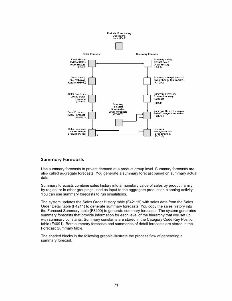
Summary Forecasts
Use summary forecasts to project demand at a product group level. Summary forecasts are also called aggregate forecasts. You generate a summary forecast based on summary actual data.
Summary forecasts combine sales history into a monetary value of sales by product family, by region, or in other groupings used as input to the aggregate production planning activity. You can use summary forecasts to run simulations.
The system updates the Sales Order History table (F42119) with sales data from the Sales Order Detail table (F4211) to generate summary forecasts. You copy the sales history into the Forecast Summary table (F3400) to generate summary forecasts. The system generates summary forecasts that provide information for each level of the hierarchy that you set up with summary constants. Summary constants are stored in the Category Code Key Position table (F4091). Both summary forecasts and summaries of detail forecasts are stored in the Forecast Summary table.
The shaded blocks in the following graphic illustrate the process flow of generating a summary forecast.
71
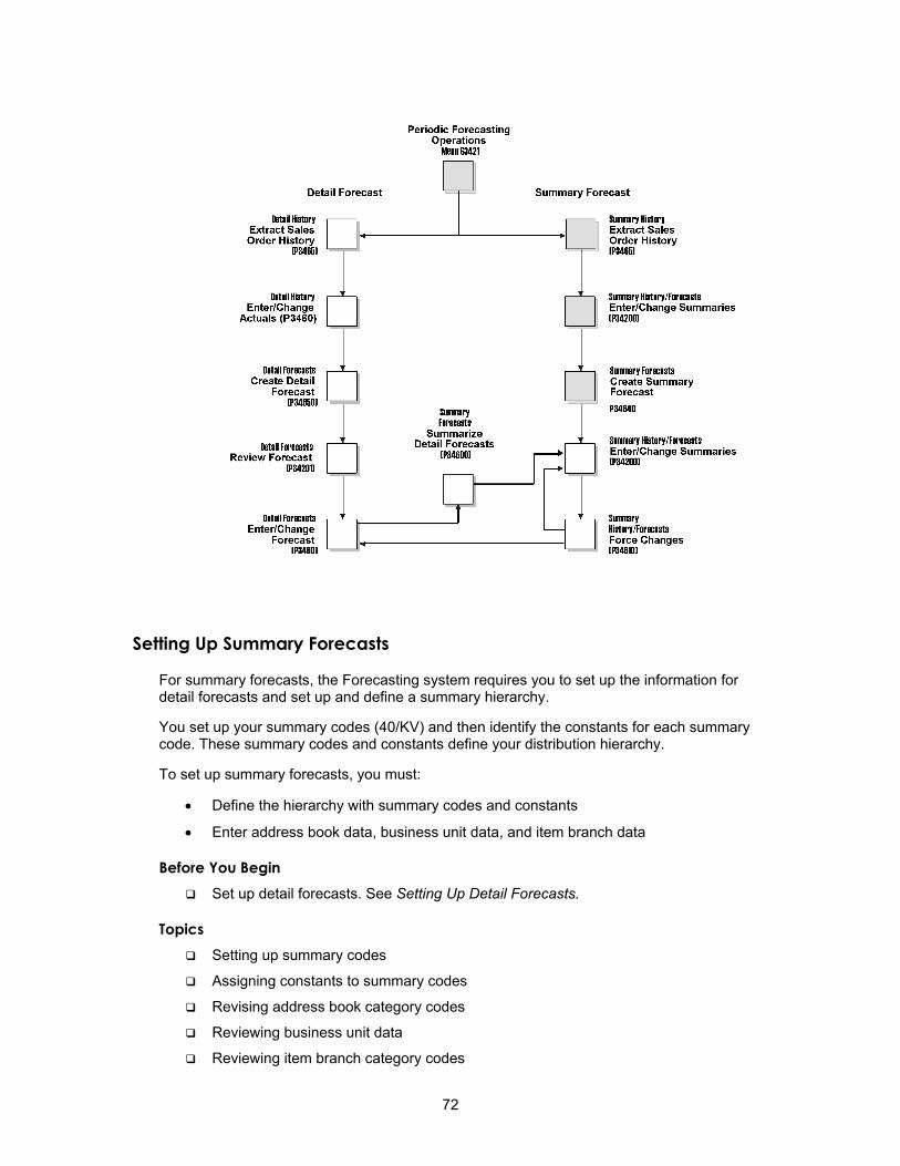
Setting Up Summary Forecasts
For summary forecasts, the Forecasting system requires you to set up the information for detail forecasts and set up and define a summary hierarchy.
You set up your summary codes (40/KV) and then identify the constants for each summary code. These summary codes and constants define your distribution hierarchy.
To set up summary forecasts, you must:
• Define the hierarchy with summary codes and constants
• Enter address book data, business unit data, and item branch data
Before You Begin Set up detail forecasts. See Setting Up Detail Forecasts.
Topics Setting up summary codes
Assigning constants to summary codes
Revising address book category codes
Reviewing business unit data
Reviewing item branch category codes
72
Setting Up Summary Codes
To set up the hierarchy, you must set up summary codes and summary constants. For each hierarchy you define, you must specify a unique identifier called a summary code. For example, you can use summary code 999 to represent a hierarchy called Summarization by Region. When creating summary forecasts, you choose a summary code to indicate which hierarchy you want to work with.
Before You Begin Update the sales history. See Updating Customer Sales in the Sales Order
Management Guide.
See Also About User Defined Codes in the OneWorld Foundation Guide for more information
about user defined codes
Assigning Constants to Summary Codes
For each summary code, use summary constants to define each level of the hierarchy. You can use category codes from the Address Book Revision program (P01012) and Item Master table (F4101) to define up to 14 levels in the hierarchy. You can define these levels as follows:
• Define the top level as the Global Summary to summarize forecasts for several companies into a single corporate view.
• Define the second level as the Company Summary to summarize forecasts for all facilities in a single company.
• Define up to 11 middle levels, which include the category codes and the customer level.
• Use as many as 20 address book category codes and 20 item branch category codes to assign other levels in the hierarchy.
• Use the Customer Level field as another category code. You can specify each of your large customers as a level of the hierarchy. This action allows you to create specific forecasts for each large customer.
• The lowest level you can define is the item level.
• Define an Item Summary level that provides forecasts for the individual item level. All detail forecast records for an item can be summarized at this level.
Detail records for a branch/plant item are automatically placed after all levels of the hierarchy. The system does not include these detail records as one of the 14 levels of the hierarchy.
► To assign constants to summary codes
From the Forecasting Setup menu (G3441), choose Summary Constants.
73
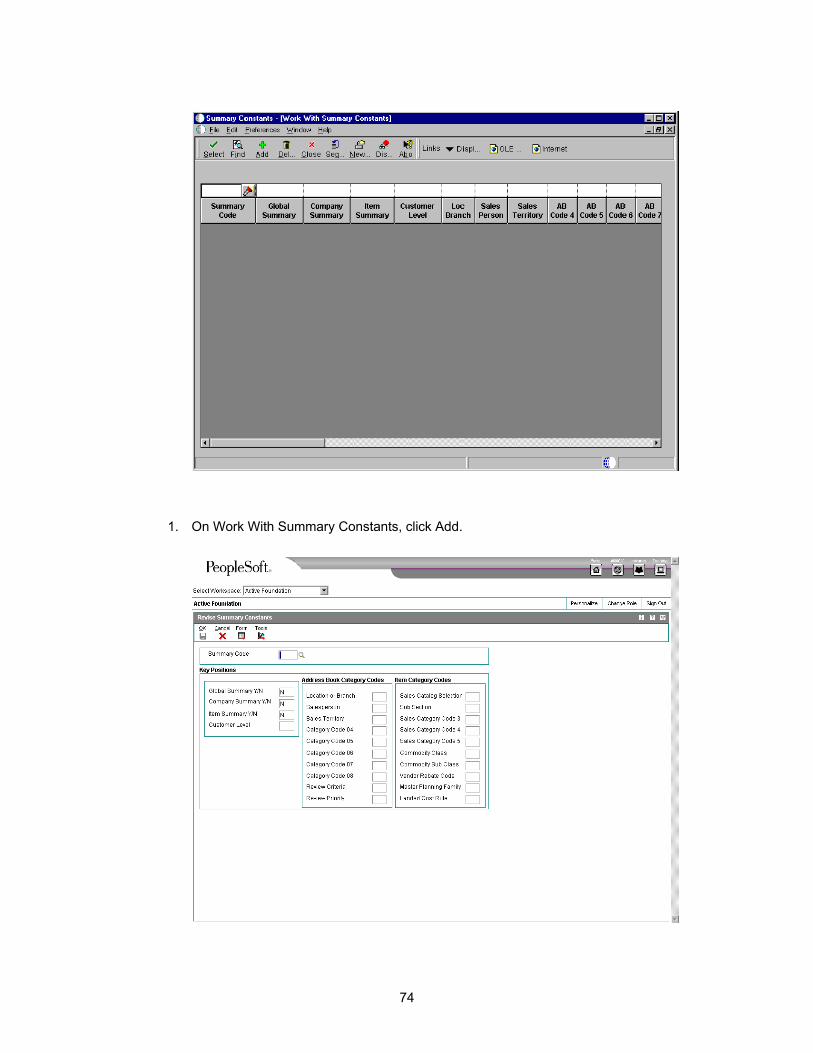
1. On Work With Summary Constants, click Add.
74
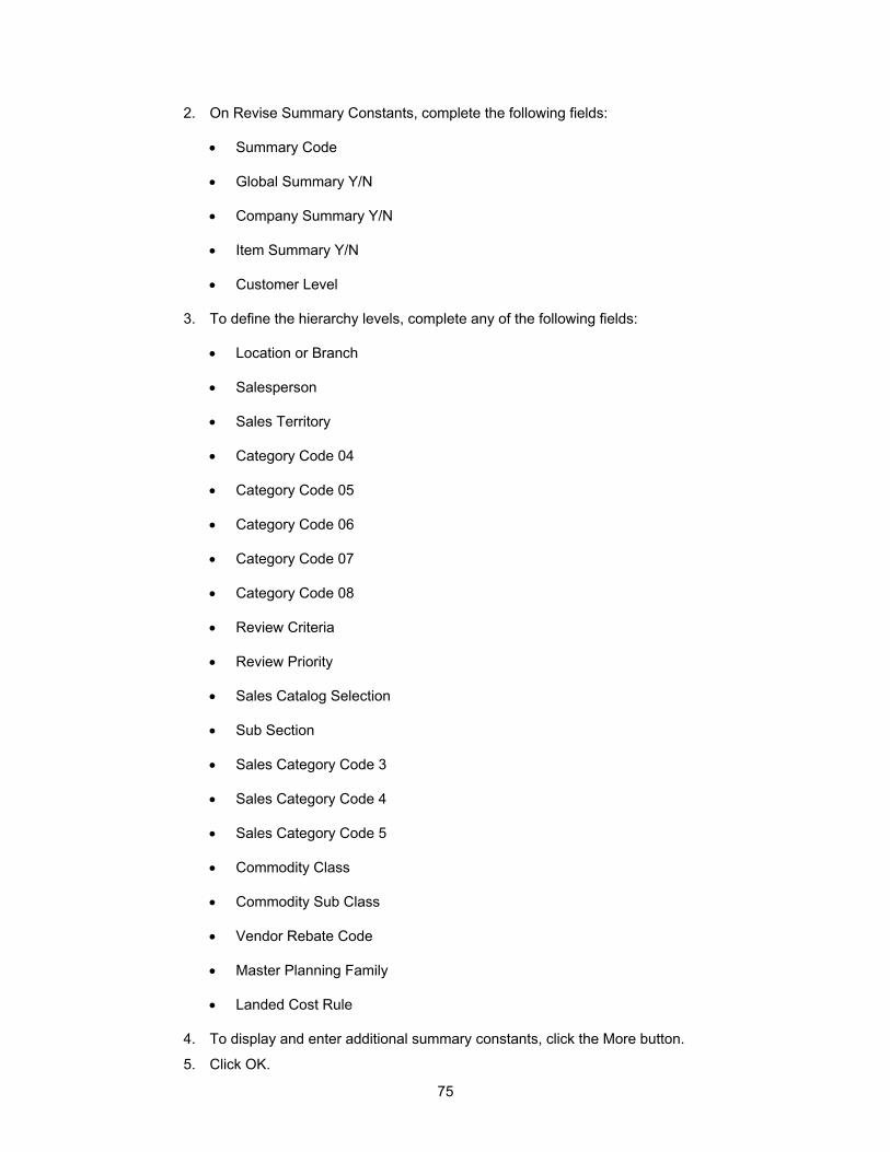
2. On Revise Summary Constants, complete the following fields:
• Summary Code
• Global Summary Y/N
• Company Summary Y/N
• Item Summary Y/N
• Customer Level
3. To define the hierarchy levels, complete any of the following fields:
• Location or Branch
• Salesperson
• Sales Territory
• Category Code 04
• Category Code 05
• Category Code 06
• Category Code 07
• Category Code 08
• Review Criteria
• Review Priority
• Sales Catalog Selection
• Sub Section
• Sales Category Code 3
• Sales Category Code 4
• Sales Category Code 5
• Commodity Class
• Commodity Sub Class
• Vendor Rebate Code
• Master Planning Family
• Landed Cost Rule
4. To display and enter additional summary constants, click the More button.
5. Click OK.
75
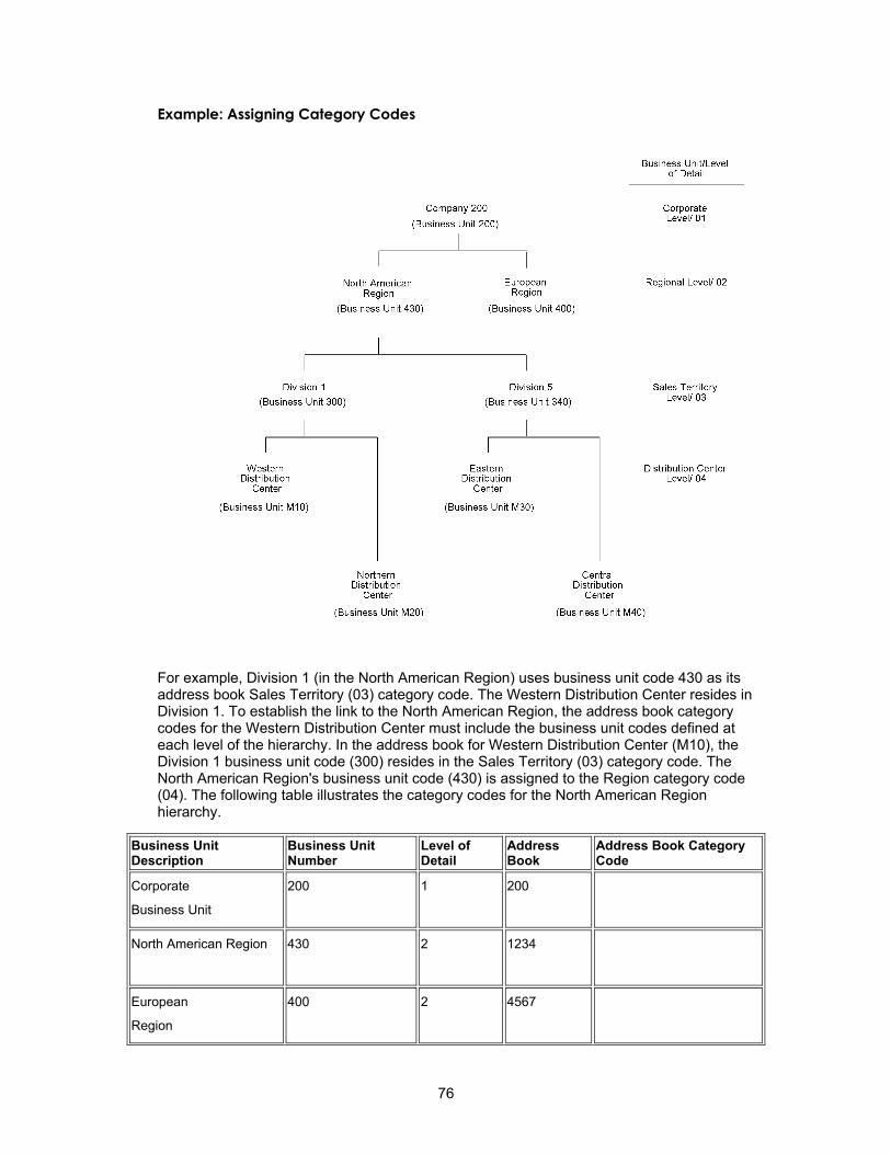
Example: Assigning Category Codes
For example, Division 1 (in the North American Region) uses business unit code 430 as its address book Sales Territory (03) category code. The Western Distribution Center resides in Division 1. To establish the link to the North American Region, the address book category codes for the Western Distribution Center must include the business unit codes defined at each level of the hierarchy. In the address book for Western Distribution Center (M10), the Division 1 business unit code (300) resides in the Sales Territory (03) category code. The North American Region's business unit code (430) is assigned to the Region category code (04). The following table illustrates the category codes for the North American Region hierarchy.
Business Unit Description
Business Unit Number
Level of Detail
Address Book
Address Book Category Code
Corporate
Business Unit
200 1 200
North American Region 430 2 1234
European
Region
400 2 4567
76
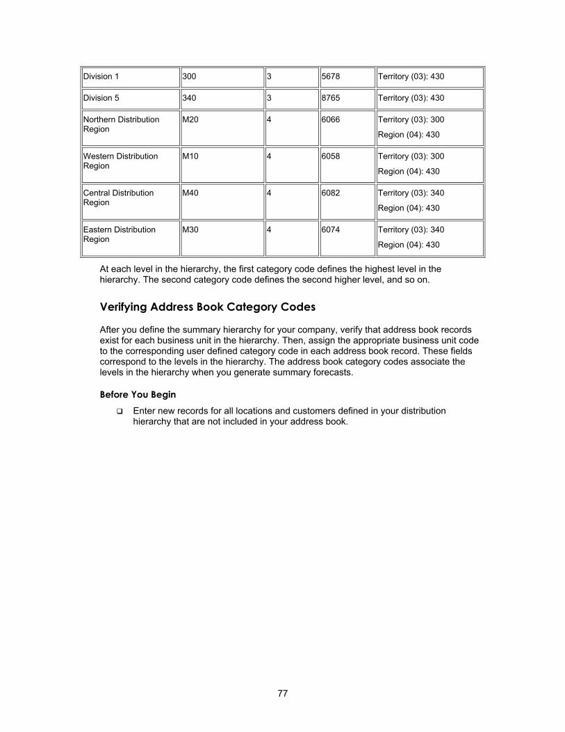
Division 1 300 3 5678 Territory (03): 430
Division 5 340 3 8765 Territory (03): 430
Northern Distribution Region
M20 4 6066 Territory (03): 300
Region (04): 430
Western Distribution Region
M10 4 6058 Territory (03): 300
Region (04): 430
Central Distribution Region
M40 4 6082 Territory (03): 340
Region (04): 430
Eastern Distribution Region
M30 4 6074 Territory (03): 340
Region (04): 430
At each level in the hierarchy, the first category code defines the highest level in the hierarchy. The second category code defines the second higher level, and so on.
Verifying Address Book Category Codes
After you define the summary hierarchy for your company, verify that address book records exist for each business unit in the hierarchy. Then, assign the appropriate business unit code to the corresponding user defined category code in each address book record. These fields correspond to the levels in the hierarchy. The address book category codes associate the levels in the hierarchy when you generate summary forecasts.
Before You Begin Enter new records for all locations and customers defined in your distribution
hierarchy that are not included in your address book.
77
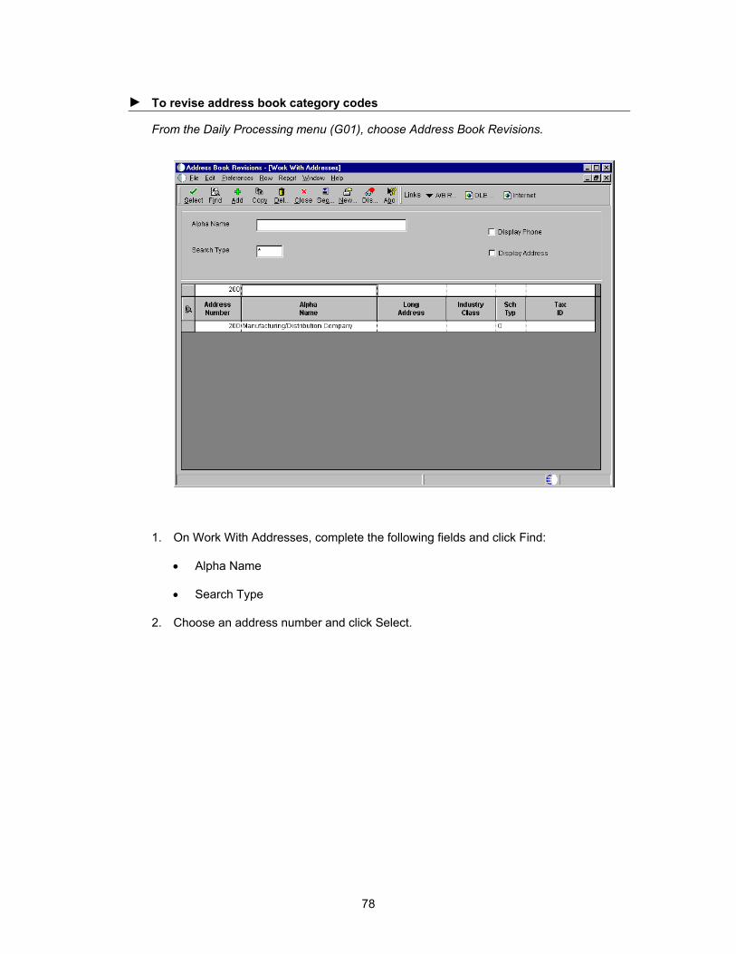
► To revise address book category codes
From the Daily Processing menu (G01), choose Address Book Revisions.
1. On Work With Addresses, complete the following fields and click Find:
• Alpha Name
• Search Type
2. Choose an address number and click Select.
78
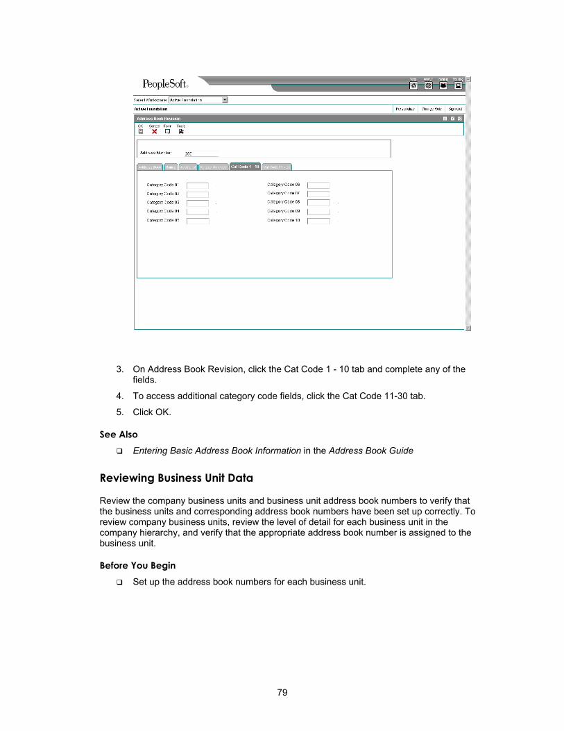
3. On Address Book Revision, click the Cat Code 1 - 10 tab and complete any of the fields.
4. To access additional category code fields, click the Cat Code 11-30 tab.
5. Click OK.
See Also Entering Basic Address Book Information in the Address Book Guide
Reviewing Business Unit Data
Review the company business units and business unit address book numbers to verify that the business units and corresponding address book numbers have been set up correctly. To review company business units, review the level of detail for each business unit in the company hierarchy, and verify that the appropriate address book number is assigned to the business unit.
Before You Begin Set up the address book numbers for each business unit.
79
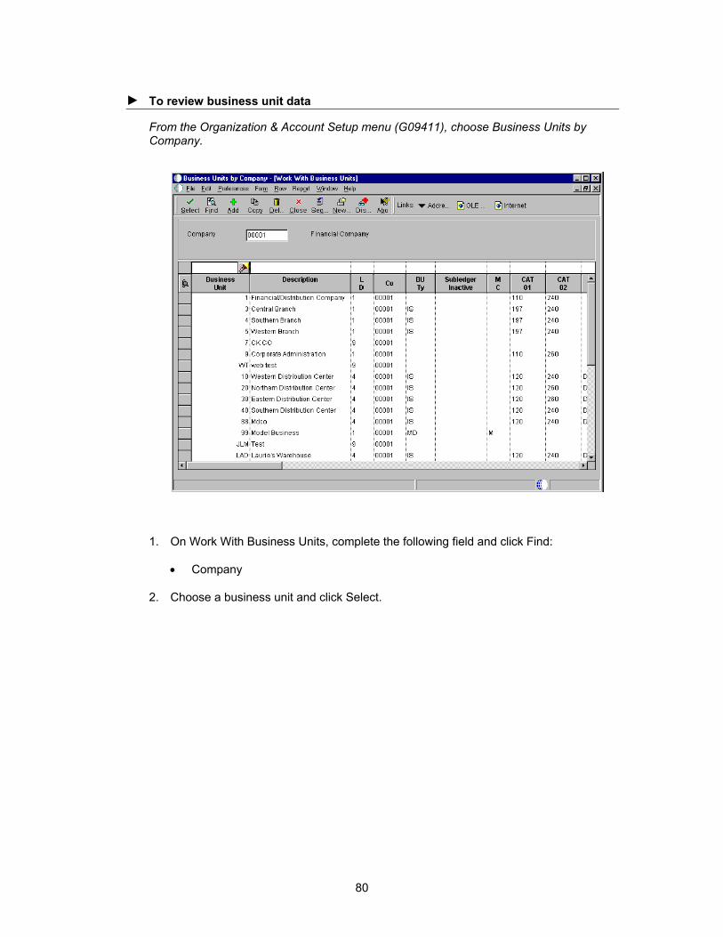
► To review business unit data
From the Organization & Account Setup menu (G09411), choose Business Units by Company.
1. On Work With Business Units, complete the following field and click Find:
• Company
2. Choose a business unit and click Select.
80
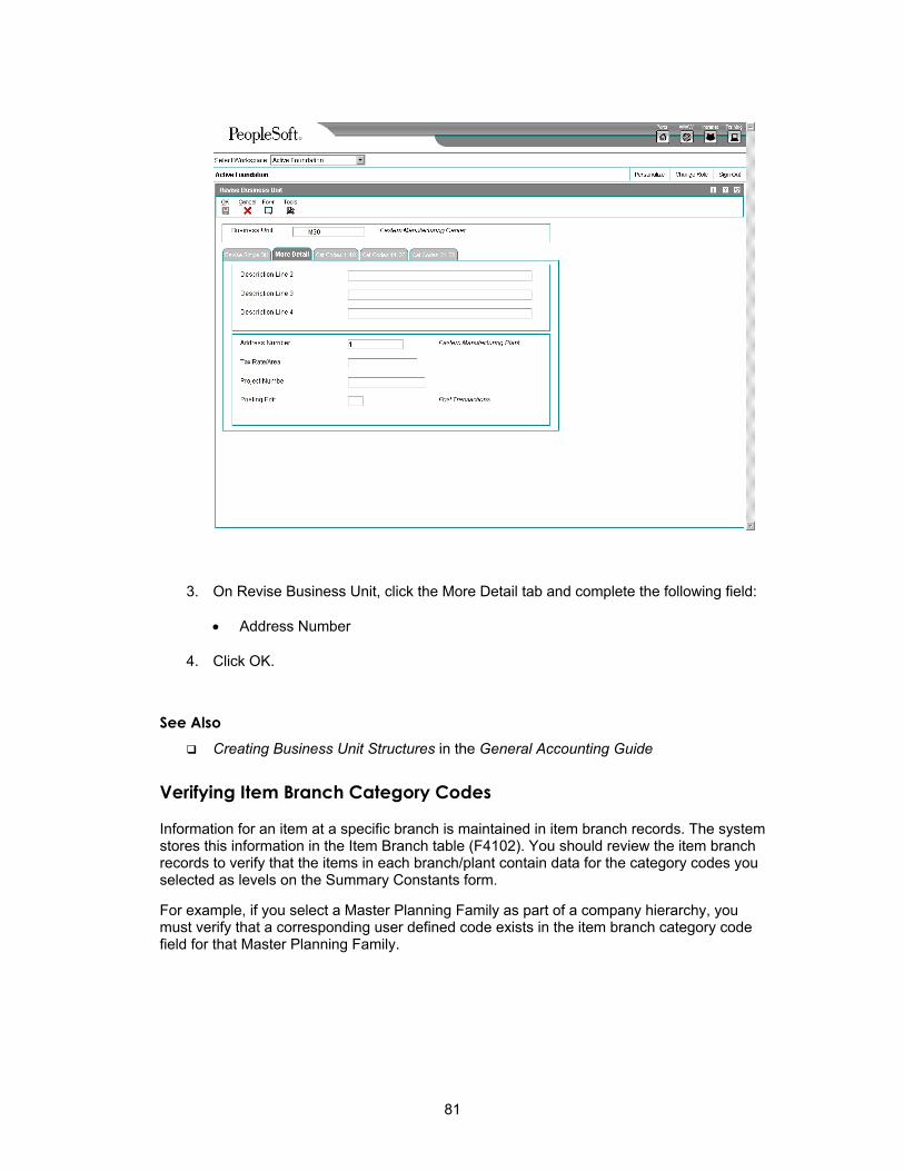
3. On Revise Business Unit, click the More Detail tab and complete the following field:
• Address Number
4. Click OK.
See Also Creating Business Unit Structures in the General Accounting Guide
Verifying Item Branch Category Codes
Information for an item at a specific branch is maintained in item branch records. The system stores this information in the Item Branch table (F4102). You should review the item branch records to verify that the items in each branch/plant contain data for the category codes you selected as levels on the Summary Constants form.
For example, if you select a Master Planning Family as part of a company hierarchy, you must verify that a corresponding user defined code exists in the item branch category code field for that Master Planning Family.
81
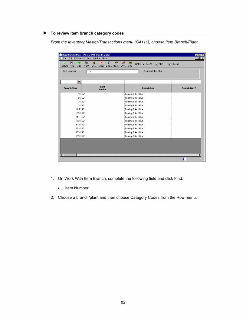
► To review item branch category codes
From the Inventory Master/Transactions menu (G4111), choose Item Branch/Plant.
1. On Work With Item Branch, complete the following field and click Find:
• Item Number
2. Choose a branch/plant and then choose Category Codes from the Row menu.
82
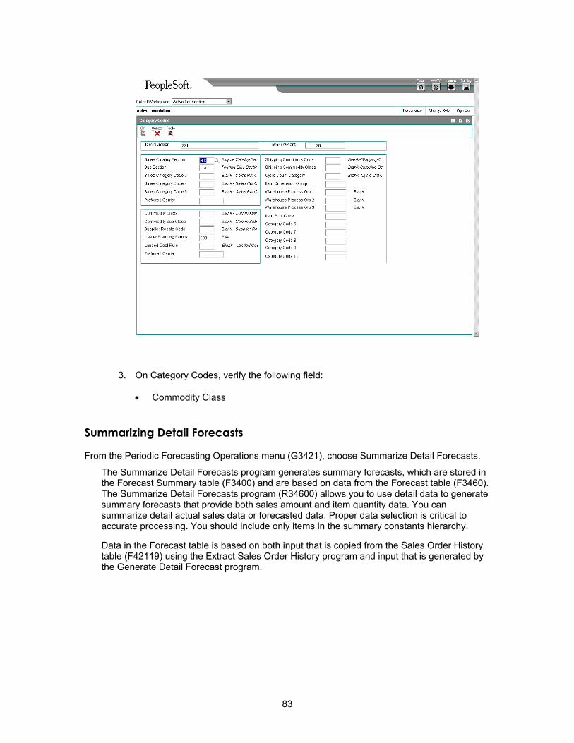
3. On Category Codes, verify the following field:
• Commodity Class
Summarizing Detail Forecasts
From the Periodic Forecasting Operations menu (G3421), choose Summarize Detail Forecasts.
The Summarize Detail Forecasts program generates summary forecasts, which are stored in the Forecast Summary table (F3400) and are based on data from the Forecast table (F3460). The Summarize Detail Forecasts program (R34600) allows you to use detail data to generate summary forecasts that provide both sales amount and item quantity data. You can summarize detail actual sales data or forecasted data. Proper data selection is critical to accurate processing. You should include only items in the summary constants hierarchy.
Data in the Forecast table is based on both input that is copied from the Sales Order History table (F42119) using the Extract Sales Order History program and input that is generated by the Generate Detail Forecast program.
83
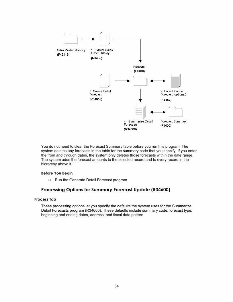
You do not need to clear the Forecast Summary table before you run this program. The system deletes any forecasts in the table for the summary code that you specify. If you enter the from and through dates, the system only deletes those forecasts within the date range. The system adds the forecast amounts to the selected record and to every record in the hierarchy above it.
Before You Begin Run the Generate Detail Forecast program.
Processing Options for Summary Forecast Update (R34600)
Process Tab These processing options let you specify the defaults the system uses for the Summarize Detail Forecasts program (R34600). These defaults include summary code, forecast type, beginning and ending dates, address, and fiscal date pattern.
84
The Summarize Detail Forecasts program generates summary forecasts based on data from the Forecast table (F3460), and stores the forecasts in the Forecast Summary table (F3400). The summary forecasts provide both sales amount and item quantity data. You can summarize Detail Actual Sales data or forecasted data. Proper data selection is critical to accurate processing. You should include only items in the summary constants hierarchy.
Summary Code
Use this processing option to specify which summary code the system uses when
running the summary. Summary code is a user defined code (40/KV) that
identifies the summary code for running the summary. You define summary codes
using the Summary Constants program (P4091) from the Forecasting Setup menu
(G3441). Enter the summary code to use as the default value or choose it from
the Select User Define Code form.
Forecast Type
Use this processing option to specify the detail forecast type that you want
the system to use to summarize the forecast. Forecast type is a user defined
code (34/DF) that identifies the detail forecast type. Enter the forecast type
to use as the default value or choose it from the Select User Define Code
form.
From Date
Blank = Use all data
Enter a Date
Use this processing option to specify the date from which the system begins
the summary forecast. Enter a date to use as the beginning forecast date or
choose a date from the calendar. If you leave this field blank, the system
uses all data to generate the summary forecast.
85
Thru Date
Blank = Use all data
Enter a Date
Use this processing option to specify the date from which the system ends the
summary forecast. Enter a date to use as the ending forecast date or choose a
date from the calendar. If you leave this field blank, the system uses all
data to generate the summary forecast.
Address
Blank = Business Unit
1 = Address
Use this processing option to specify whether the system considers the address
book numbers are part of the hierarchy or if the system retrieves the address
book numbers from the business unit associated with the forecast.
If you leave this field blank, the system retrieves the address book numbers
from the business units associated with the forecast detail. In the Business
Units program (P0006) on the Organization Account Setup menu (G09411) you can
determine which address number is assigned to a business unit. In this case,
the system uses the category codes for that address number if you are using
address book category codes in the summarization hierarchy.
If you enter 1, the system considers the address book numbers of the customers
are part of the hierarchy. This customer number comes from the Forecast table
(F3460). The customer number would be part of the forecast as a result of
generating forecasts for large customers. If you did not generate forecasts
for large customers or if you do not have any customers defined as large (ABC
code on the Customer Master table (F0301) set to A) the system does not
associate address book numbers with the forecasts.
Valid values are:
Blank The system retrieves the address book number from the business
86
units associated with the forecast detail.
1 The system considers the address book numbers of the customers are
part of the hierarchy.
Fiscal Date Pattern
Use this processing option to specify the monthly fiscal date pattern the
system uses to create summary forecasts. Fiscal date pattern is a user defined
code (H00/DP) that identifies the date pattern for the forecast. The system
retrieves the pattern from the Date Fiscal Patterns table (F0008). Enter the
fiscal date pattern to use as the default value or choose it from the Select
User Define Code form. If you leave this field blank, the system creates
records using dates from the detail forecast records.
Topics Reviewing a summary forecast
Revising a summary forecast
Revising summary forecasts using Forecast Forcing (optional)
Working with Summarized Detail Forecasts
After generating the forecasts, you can compare them to actual sales order histories. You can then revise both history and forecast data according to your own criteria.
When you review summaries of forecasts, you can also access a previously generated forecast. You can access a date range to display the sales order history and the forecast of item quantities or sales amounts. Then, you can compare actual sales to the forecast.
When you revise summaries of forecasts, you revise information in a specific level of the forecast. You can also use the Force Changes program to apply changes you made to the summary. You can apply these changes up the hierarchy, down the hierarchy, or in both directions.
Before You Begin Generate a summary forecast or a summary of detail forecast. See Summarizing
Detail Forecasts or Generating Summary Forecasts.
87
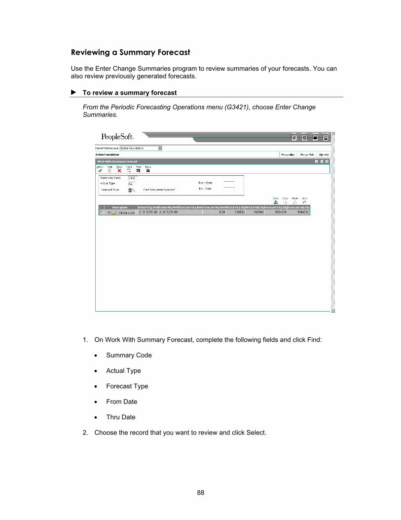
Reviewing a Summary Forecast
Use the Enter Change Summaries program to review summaries of your forecasts. You can also review previously generated forecasts.
► To review a summary forecast
From the Periodic Forecasting Operations menu (G3421), choose Enter Change Summaries.
1. On Work With Summary Forecast, complete the following fields and click Find:
• Summary Code
• Actual Type
• Forecast Type
• From Date
• Thru Date
2. Choose the record that you want to review and click Select.
88
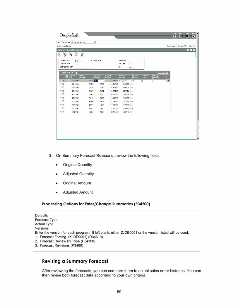
3. On Summary Forecast Revisions, review the following fields:
• Original Quantity
• Adjusted Quantity
• Original Amount
• Adjusted Amount
Processing Options for Enter/Change Summaries (P34200)
Defaults Forecast Type Actual Type Versions Enter the version for each program. If left blank, either ZJDE0001 or the version listed will be used. 1. Forecast Forcing (XJDE0001) (R34610) 2. Forecast Review By Type (P34300) 3. Forecast Revisions (P3460)
Revising a Summary Forecast
After reviewing the forecasts, you can compare them to actual sales order histories. You can then revise both forecast data according to your own criteria.
89
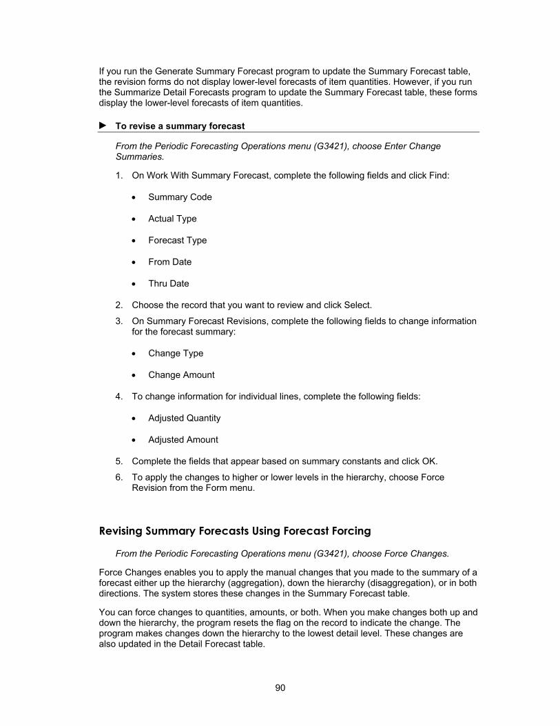
If you run the Generate Summary Forecast program to update the Summary Forecast table, the revision forms do not display lower-level forecasts of item quantities. However, if you run the Summarize Detail Forecasts program to update the Summary Forecast table, these forms display the lower-level forecasts of item quantities.
► To revise a summary forecast
From the Periodic Forecasting Operations menu (G3421), choose Enter Change Summaries.
1. On Work With Summary Forecast, complete the following fields and click Find:
• Summary Code
• Actual Type
• Forecast Type
• From Date
• Thru Date
2. Choose the record that you want to review and click Select.
3. On Summary Forecast Revisions, complete the following fields to change information for the forecast summary:
• Change Type
• Change Amount
4. To change information for individual lines, complete the following fields:
• Adjusted Quantity
• Adjusted Amount
5. Complete the fields that appear based on summary constants and click OK.
6. To apply the changes to higher or lower levels in the hierarchy, choose Force Revision from the Form menu.
Revising Summary Forecasts Using Forecast Forcing
From the Periodic Forecasting Operations menu (G3421), choose Force Changes.
Force Changes enables you to apply the manual changes that you made to the summary of a forecast either up the hierarchy (aggregation), down the hierarchy (disaggregation), or in both directions. The system stores these changes in the Summary Forecast table.
You can force changes to quantities, amounts, or both. When you make changes both up and down the hierarchy, the program resets the flag on the record to indicate the change. The program makes changes down the hierarchy to the lowest detail level. These changes are also updated in the Detail Forecast table.
90
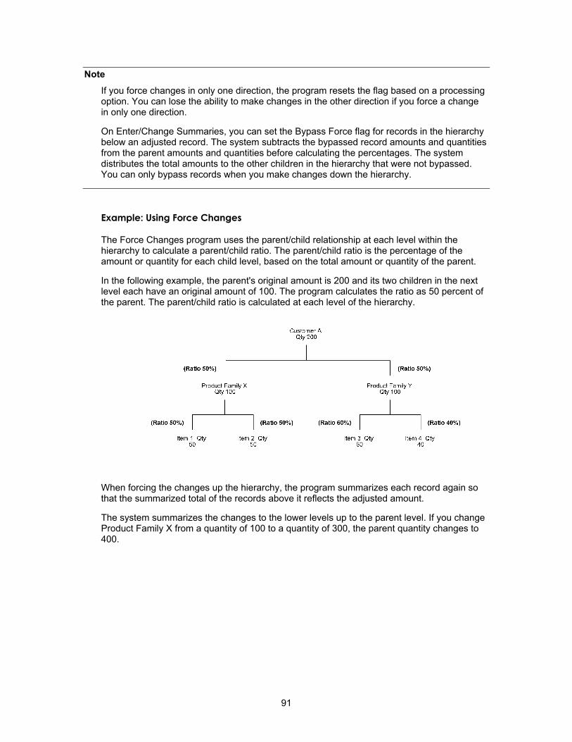
Note If you force changes in only one direction, the program resets the flag based on a processing option. You can lose the ability to make changes in the other direction if you force a change in only one direction.
On Enter/Change Summaries, you can set the Bypass Force flag for records in the hierarchy below an adjusted record. The system subtracts the bypassed record amounts and quantities from the parent amounts and quantities before calculating the percentages. The system distributes the total amounts to the other children in the hierarchy that were not bypassed. You can only bypass records when you make changes down the hierarchy.
Example: Using Force Changes
The Force Changes program uses the parent/child relationship at each level within the hierarchy to calculate a parent/child ratio. The parent/child ratio is the percentage of the amount or quantity for each child level, based on the total amount or quantity of the parent.
In the following example, the parent's original amount is 200 and its two children in the next level each have an original amount of 100. The program calculates the ratio as 50 percent of the parent. The parent/child ratio is calculated at each level of the hierarchy.
When forcing the changes up the hierarchy, the program summarizes each record again so that the summarized total of the records above it reflects the adjusted amount.
The system summarizes the changes to the lower levels up to the parent level. If you change Product Family X from a quantity of 100 to a quantity of 300, the parent quantity changes to 400.
91
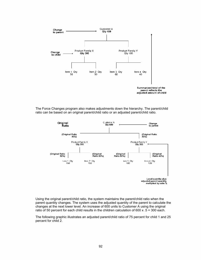
The Force Changes program also makes adjustments down the hierarchy. The parent/child ratio can be based on an original parent/child ratio or an adjusted parent/child ratio.
Using the original parent/child ratio, the system maintains the parent/child ratio when the parent quantity changes. The system uses the adjusted quantity of the parent to calculate the changes at the next lower level. An increase of 600 units to Customer A using the original ratio of 50 percent for each child results in the children calculation of 600 x .5 = 300 each.
The following graphic illustrates an adjusted parent/child ratio of 75 percent for child 1 and 25 percent for child 2.
92
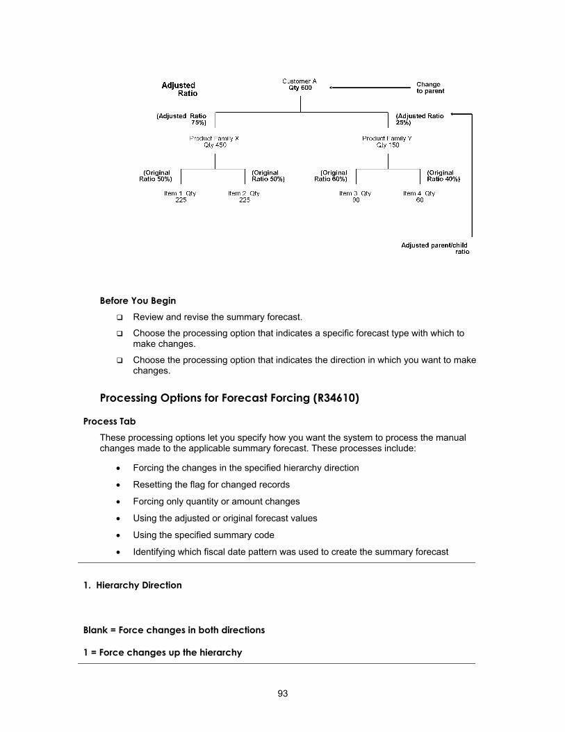
Before You Begin Review and revise the summary forecast.
Choose the processing option that indicates a specific forecast type with which to make changes.
Choose the processing option that indicates the direction in which you want to make changes.
Processing Options for Forecast Forcing (R34610)
Process Tab These processing options let you specify how you want the system to process the manual changes made to the applicable summary forecast. These processes include:
• Forcing the changes in the specified hierarchy direction
• Resetting the flag for changed records
• Forcing only quantity or amount changes
• Using the adjusted or original forecast values
• Using the specified summary code
• Identifying which fiscal date pattern was used to create the summary forecast
1. Hierarchy Direction
Blank = Force changes in both directions
1 = Force changes up the hierarchy
93
2 = Force changes down the hierarchy
Use this processing option to specify the direction in which to force the
changes made to the summary forecast. The system updates the changes in the
Forecast table (F3460).
Blank The system forces the changes up and down the hierarchy and
automatically resets the flag on the record to indicate the change.
1 The system forces the changes up the hierarchy.
2 The system forces the changes down the hierarchy.
If you set this processing option to 1 or 2 and you want the system to reset
the flag on the changed record, set the Revised Flag processing option to 1.
2. Revised Flag
Blank = Do not reset the Revised Flag
1 = Reset the Revised flag
Use this processing option to specify whether the system resets the revised
flag for the records changed when you set the Hierarchy Direction processing
option to 1 or 2.
Blank The system does not reset the Revised flag.
1 The system resets the Revised flag for the changed record.
3. Quantities and Amounts
Blank = Force changes to quantities and amounts
1 = Force quantity changes only
2 = Force amount changes only
Use this processing option to specify whether the system forces the changes
94
made to quantities or amounts or both.
Blank The system forces the changes made to both quantities and amounts.
1 The system forces only the quantity changes.
2 The system forces only the amount changes.
4. Ratio Calculations
Blank = Use original forecast values
1 = Use adjusted forecast values
Use this processing option to specify whether the system calculates the
parent/child ratios using the original or the adjusted forecast values. The
parent/child ratio is the percentage of the amount or quantity for each child
level, based on the total amount or quantity of the parent.
Blank The system uses the original forecast values.
1 The system uses the adjusted forecast values.
5. Summary Code (Required)
Use this processing option to specify the summary code for which to force
changes. This processing option is required and the system overrides any
summary code specified in the data selection. Summary code is a user defined
code (40/KV) that identifies the summary code. You define summary codes using
the Summary Constants program (P4091) from the Forecasting Setup menu (G3441).
Enter the summary code to use or choose it from the Select User Define Code
form.
6. Fiscal Date Pattern
Use this processing option to specify the fiscal date pattern used to create
this summary forecast. This processing option is required if you set the
95
Hierarchy Direction processing option to force changes down and if you created
the summary and detail forecasts using different fiscal date patterns. Fiscal
date pattern is a user defined code (H00/DP) that identifies the date pattern
for the forecast. The system retrieves the pattern from the Date fiscal
Patterns table (F0008). Enter the fiscal date pattern to use or choose it from
the Select User Define Code form. If you leave this field blank, the system
forces the changes both up and down the hierarchy.
Generating Summary Forecasts
The system generates summary forecasts based on sales history data that you copy from the Sales Order History table (F42119) into the Forecast Summary table (F3400). When you copy the sales history, you specify a date range based on the request date of the sales order. The sales history data can be distorted by unusually large or small values (spikes or outliers), data entry errors, or missing demand (sales orders that were cancelled due to lack of inventory).
You should review the data in the date range you specified to identify missing or inaccurate information. You then revise the sales order history to account for inconsistencies and distortions when you generate the forecast. If you want to account for changes in sales order activity for an especially large customer, the J.D. Edwards Forecasting system allows you to work with that customer's changes separately.
Note To generate summary forecasts for item quantities on all levels of the hierarchy, first generate a detail forecast, then run the Summarize Detail Forecasts program.
Topics Copying summary sales order history
Creating a summary forecast
Revising sales order history
Copying Summary Sales Order History
From the Periodic Forecasting Operations menu (G3421), choose Extract Sales Actuals.
The system generates summary forecasts based on data in the Forecast Summary table. Use Extract Sales Order History to copy the sales order history (type AA) from the Sales Order History table to the Forecast Summary table based upon criteria that you specify.
96
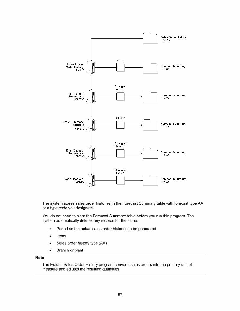
The system stores sales order histories in the Forecast Summary table with forecast type AA or a type code you designate.
You do not need to clear the Forecast Summary table before you run this program. The system automatically deletes any records for the same:
• Period as the actual sales order histories to be generated
• Items
• Sales order history type (AA)
• Branch or plant
Note The Extract Sales Order History program converts sales orders into the primary unit of measure and adjusts the resulting quantities.
97
Before You Begin Set up detail forecasts. See Setting Up Detail Forecasts.
Set up the summary forecast. See Setting Up Summary Forecasts.
See Also Creating Customer Records in the Accounts Receivable Guide
Copying Sales Order History to review the processing options for Extract Sales Actuals
Creating a Summary Forecast
From the Periodic Forecasting Operations menu (G3421), choose Create Summary Forecast.
The Generate Summary Forecast program allows you to test simulated versions of future sales scenarios without having to run full detail forecasts. You can use this program to simulate and plan long-range trends because this program does not update information in the Forecast table, which is used as input to DRP, MPS, and MRP generation.
You can simulate multiple forecasting methods, including the system's 12 hard-coded methods, with past sales order histories and then select the best fit as determined by the system or another appropriate model to generate a forecast of future sales amounts. You can also select a specific forecasting method and use that model to generate the current forecast. The system generates forecasts of sales amounts for each level in the hierarchy and stores them in the Forecast Summary table.
The Generate Summary Forecast program uses the same 12 forecasting methods used to create detail forecasts. However, the system creates forecast information for each level in the hierarchy.
You can also use the Generate Summary Forecast program to:
• Specify the summary code for the hierarchy for which you want to forecast
• Generate summary forecasts based on sales history
• Select a best fit forecast
• Store any or all of the forecast methods in the Forecast Summary table
• Generate the forecast in a fiscal date pattern you select
• Specify the number of months of actual data to use to create the best fit
• Forecast for individual large customers
• Forecast an unlimited number of periods into the future
If you use the default type codes in the processing options, the actual sales history records are identified by type AA, and the best fit model is identified by type BF. The system saves the BF type and AA type records (or corresponding type codes that you designate) in the Forecast Summary table. However, forecast types 01 through 12 are not automatically saved. You must set a processing option to save them.
When you run the Generate Summary Forecast program, the system:
• Extracts sales order history information from the Forecast Summary table
• Calculates the forecasts using methods that you select
98
• Determines the percent of accuracy or Mean Absolute Deviation (MAD) for each selected forecast method
• Recommends the best fit forecast method
• Generates the summary forecast in both monetary amounts and units from the best fit forecast
See Also
• R34640, Create Summary Forecasts in the Reports Guide for a report sample
Before You Begin Run the Extract Sales Order History program.
Make changes to the sales order history with the Enter/Change Actuals program.
On Generate Summary Forecast, set the Dollar/Unit Forecast processing option to the value that means forecast summary amounts.
Processing Options for Create Summary Forecast (R34640)
Methods 1 - 3 Tab These processing options let you specify which forecast types the system uses when calculating the best fit forecast for each level in the hierarchy. You can also specify whether the system creates summary forecasts for the selected forecast method.
Enter 1 to use the forecast method when calculating the best fit. If you leave the processing option blank, the system does not use that forecast method when calculating the best fit and does not create summary forecasts for the method.
The system defines a period as a week or month, depending on the pattern selected from the Date Fiscal Patterns table (F0008). For weekly forecasts, verify that you have established 52 period dates.
1. Percent Over Last Year
Blank = Do not use this method
1 = Use this method to create a forecasts
Use this processing option to specify which type of forecast to run. This
forecast method uses the Percent Over Last Year formula to multiply each
forecast period by a percentage increase or decrease. You specify the increase
or decrease in the Percent processing option. This method requires the periods
for the best fit plus one year of sales history. This method is useful for
seasonal items with growth or decline. Valid values are:
99
Blank The system does not use this method.
1 The system uses the Percent Over Last Year formula to create
summary forecasts.
2. Percent
Use this processing option to specify the percent of increase or decrease by
which the system multiplies the sales history from last year. For example,
type 110 for a 10 percent increase or type 97 for a 3 percent decrease. Valid
values are any percent amount; however, the amount cannot be a negative
amount. Enter an amount to use or choose it from the Calculator.
3. Calculated Percent Over Last Year
Blank = Do not use this method
1 = Use this method to create forecasts
Use this processing option to specify which type of forecast to run. This
forecast method uses the Calculated Percent Over Last Year formula to compare
the periods of past sales that you specify to the same periods of past sales
of the previous year. The system determines a percentage increase or decrease,
then multiplies each period by this percentage to determine the forecast. This
method uses the periods of sales order history that you specify in the
following Number of Periods processing option plus one year of sales history.
This method is useful for short-term demand forecasts of seasonal items with
growth or decline. Valid values are:
Blank The system does not use this method.
1 The system uses the Calculated Percent Over Last Year formula to
create summary forecasts.
4. Number of Periods
100
Use this processing option to specify the number of periods to include when
calculating the percentage increase or decrease. Enter a number to use or
choose it from the Calculator.
5. Last Year to This Year
Blank = Do not use this method
1 = Use this method to create forecasts
Use this processing option to specify which type of forecast to run. This
forecast method uses the Last Year to This Year formula which calculates the
year's forecast based on the prior year's sales. This method uses the periods
best fit plus one year of sales order history. This method is useful for
mature products with level demand or seasonal demand without a trend. Valid
values are:
Blank The system does not use this method.
1 The system uses the Last Year to This Year formula to create
summary forecasts.
Methods 4 - 6 Tab These processing options let you specify which forecast types the system uses when calculating the best fit forecast for each level in the hierarchy. You can also specify whether the system creates summary forecasts for the selected forecast method.
Enter 1 to use the forecast method when calculating the best fit. If you leave the processing option blank, the system does not use that forecast method when calculating the best fit and does not create summary forecasts for the method.
101
The system defines a period as a week or month, depending on the pattern selected from the Date Fiscal Patterns table (F0008). For weekly forecasts, verify that you have established 52 period dates.
1. Moving Average Blank = Do not use this method 1 = Use this method to create forecasts Use this processing option to specify which type of forecast to run. This
forecast method uses the Moving Average formula to average the months that you
indicate in the following Number of Periods processing option to project the
next period. This method uses the periods for the best fit from the Actual
Data processing option under the Process 1 tab plus the number of periods of
sales order history. You should have the system recalculate this forecast
monthly or at least quarterly to reflect changing demand level. This method is
useful for mature products without a trend. Valid values are:
Blank The system does not use this method.
1 The system uses the Moving Average formula to create summary
forecasts.
2. Number of Periods Use this processing option to specify the number of periods to include in the
Moving Average forecast method. Enter a number to use or choose it from the
Calculator.
3. Linear Approximation Blank = Do not use this method 1 = Use this method to create forecasts Use this processing option to specify which type of forecast to run. This
forecast method uses the Linear Approximation formula to compute a trend from
the periods of sales order history and projects this trend to the forecast.
You should have the system recalculate the trend monthly to detect changes in
102
trends. This method uses period's best fit plus the number of periods that you
indicate in the following Number of Periods processing option of sales order
history. This method is useful for new products or products with consistent
positive or negative trends that are not due to seasonal fluctuations. Valid
values are:
Blank The system does not use this method.
1 The system uses the Linear Approximation formula to create summary
forecasts.
4. Number of Periods Use this processing option to specify the number of periods to include in the
Linear Approximation forecast method. Enter the number to use or choose it
from the Calculator.
5. Least Squares Regression Blank = Do not use this method 1 = Use this method to create forecasts Use this processing option to specify which type of forecast to run. This
forecast method derives an equation describing a straight-line relationship
between the historical sales data and the passage of time. Least Squares
Regression fits a line to the selected range of data such that the sum of the
squares of the differences between the actual sales data points and the
regression line are minimized. The forecast is a projection of this straight
line into the future. This method is useful when there is a linear trend in
the sales data. This method uses sales data history for the period represented
by the number of periods best fit plus the number of historical data periods
specified in the following Number of Periods processing option. The system
requires a minimum of two historical data points. Valid values are:
Blank The system does not use this method.
1 The system uses the Least Squares Regression formula to create
103
summary forecasts.
6. Number of Periods Use this processing option to specify the number of periods to include in the
Least Squares Regression forecast method. You must enter at least two periods.
Enter the numbers to use or choose them from the Calculator.
Methods 7 - 8 Tab These processing options let you specify which forecast types the system uses when calculating the best fit forecast for each level in the hierarchy. You can also specify whether the system creates summary forecasts for the selected forecast method.
Enter 1 to use the forecast method when calculating the best fit. If you leave the processing option blank, the system does not use that forecast method when calculating the best fit and does not create summary forecasts for the method.
The system defines a period as a week or month, depending on the pattern selected from the Date Fiscal Patterns table (F0008). For weekly forecasts, verify that you have established 52 period dates.
1. Second Degree Approximation
Blank = Do not use this metod
1 = Use this method to create forecasts
Use this processing option to specify which type of forecast to run. This
forecast method uses the Second Degree Approximation formula to plot a curve
based on a specified number of sales history periods. You specify the number
of sales history periods in the following Number of Periods processing option
to project the forecast. This method adds the period's best fit and the number
of periods, and then the sum multiplies by three. This method is not useful
for long-term forecasts. Valid values are:
Blank The system does not use this method.
1 The system uses the Second Degree Approximation formula to create
summary forecasts.
104
2. Number of Periods
Use this processing option to specify the number of periods to include in the
Second Degree Approximation forecast method. Enter the number to use or choose
it from the Calculator.
3. Flexible Method
Blank = Do not use this method
1 = Use this method to create forecasts
Use this processing option to specify which type of forecast to run. This
forecast method specifies the period's best fit block of sales order history
starting "n" months prior and a percent increase or decrease with which to
modify the forecast. This method is similar to Method 1 - Percent Over Last
Year, except that you can specify the number of periods that you use as the
base. Depending on what you select as "n", this method requires period's best
fit plus the number of periods that you specify in the following Number of
Periods processing option. This method is useful when forecasting products
with a planned trend. Valid values are:
Blank The system does not use this method.
1 The system uses the Flexible Method formula to create summary
forecasts.
4. Number of Periods
Use this processing option to specify the number of periods prior to the best
fit that you want to include in the Flexible Method calculation. Enter the
number to use or choose it from the Calculator.
5. Percent Over Prior Period
105
Use this processing option to specify the percent of increase or decrease for
the system to use. For example, type 110 for a 10 percent increase or type 97
for a 3 percent decrease. Valid values are any percent amount; however, the
amount cannot be a negative amount. Enter an amount to use or choose it from
the Calculator.
Method 9 Tab These processing options let you specify which forecast types the system uses when calculating the best fit forecast for each level in the hierarchy. You can also specify whether the system creates summary forecasts for the selected forecast method.
Enter 1 to use the forecast method when calculating the best fit. If you leave the processing option blank, the system does not use that forecast method when calculating the best fit and does not create summary forecasts for the method.
The system defines a period as a week or month, depending on the pattern selected from the Date Fiscal Patterns table (F0008). For weekly forecasts, verify that you have established 52 period dates.
1. Weighted Moving Average
Blank = Do not use this method
1 = Use this method to create forecasts
Use this processing option to specify which type of forecast to use. The
Weighted Moving Average forecast formula is similar to Method 4 - Moving
Average formula, because it averages the previous number of months of sales
history indicated in the following processing options to project the next
month's sales history. However, with this formula you use the following
processing options to assign weights for each of the prior periods (up to 12).
This method uses the number of weighted periods selected plus period's best
fit. Similar to the Moving Average, this method lags demand trends, so it is
not recommended for products with strong trends or seasonality. This method is
useful for mature products with demand that is relatively level. Valid values
are:
106
Blank The system does not use this method.
1 The system uses the Weighted Moving Average formula to create
summary forecasts.
2. One Period Prior Use this processing option to specify the weight to assign to one period prior
for calculating a moving average. The total of all the weights used in the
Weighted Moving Average calculation must equal 100. If you do not enter a
weight for a period within the specified number of periods, the system uses a
weight of zero for that period. The system does not use weights entered for
periods greater than the number of specified periods. Enter the number to use
or choose it from the Calculator.
3. Two Periods Prior Use this processing option to specify the weight to assign to two periods
prior for calculating a moving average. The total of all the weights used in
the Weighted Moving Average calculation must equal 100. If you do not enter a
weight for a period within the specified number of periods, the system uses a
weight of zero for that period. The system does not use weights entered for
periods greater than the number of specified periods. Enter the number to use
or choose it from the Calculator.
4. Three Periods Prior Use this processing option to specify the weight to assign to three periods
prior for calculating a moving average. The total of all the weights used in
the Weighted Moving Average calculation must equal 100. If you do not enter a
weight for a period within the specified number of periods, the system uses a
weight of zero for that period. The system does not use weights entered for
periods greater than the number of specified periods. Enter the number to use
or choose it from the Calculator.
107
5. Four Periods Prior Use this processing option to specify the weight to assign to four periods
prior for calculating a moving average. The total of all the weights used in
the Weighted Moving Average calculation must equal 100. If you do not enter a
weight for a period within the specified number of periods, the system uses a
weight of zero for that period. The system does not use weights entered for
periods greater than the number of specified periods. Enter the number to use
or choose it from the Calculator.
6. Five Periods Prior Use this processing option to specify the weight to assign to five periods
prior for calculating a moving average. The total of all the weights used in
the Weighted Moving Average calculation must equal 100. If you do not enter a
weight for a period within the specified number of periods, the system uses a
weight of zero for that period. The system does not use weights entered for
periods greater than the number of specified periods. Enter the number to use
or choose it from the Calculator.
7. Six Periods Prior Use this processing option to specify the weight to assign to six periods
prior for calculating a moving average. The total of all the weights used in
the Weighted Moving Average calculation must equal 100. If you do not enter a
weight for a period within the specified number of periods, the system uses a
weight of zero for that period. The system does not use weights entered for
periods greater than the number of specified periods. Enter the number to use
or choose it from the Calculator.
8. Seven Periods Prior Use this processing option to specify the weight to assign to seven periods
prior for calculating a moving average. The total of all the weights used in
the Weighted Moving Average calculation must equal 100. If you do not enter a
weight for a period within the specified number of periods, the system uses a
108
weight of zero for that period. The system does not use weights entered for
periods greater than the number of specified periods. Enter the number to use
or choose it from the Calculator.
9. Eight Periods Prior Use this processing option to specify the weight to assign to eight periods
prior for calculating a moving average. The total of all the weights used in
the Weighted Moving Average calculation must equal 100. If you do not enter a
weight for a period within the specified number of periods, the system uses a
weight of zero for that period. The system does not use weights entered for
periods greater than the number of specified periods. Enter the number to use
or choose it from the Calculator.
10. Nine Periods Prior Use this processing option to specify the weight to assign to nine periods
prior for calculating a moving average. The total of all the weights used in
the Weighted Moving Average calculation must equal 100. If you do not enter a
weight for a period within the specified number of periods, the system uses a
weight of zero for that period. The system does not use weights entered for
periods greater than the number of specified periods. Enter the number to use
or choose it from the Calculator.
11. Ten Periods Prior Use this processing option to specify the weight to assign to 10 periods prior
for calculating a moving average. The total of all the weights used in the
Weighted Moving Average calculation must equal 100. If you do not enter a
weight for a period within the specified number of periods, the system uses a
weight of zero for that period. The system does not use weights entered for
periods greater than the number of specified periods. Enter the number to use
or choose it from the Calculator.
109
12. Eleven Periods Prior Use this processing option to specify the weight to assign to 11 periods prior
for calculating a moving average. The total of all the weights used in the
Weighted Moving Average calculation must equal 100. If you do not enter a
weight for a period within the specified number of periods, the system uses a
weight of zero for that period. The system does not use weights entered for
periods greater than the number of specified periods. Enter the number to use
or choose it from the Calculator.
13. Twelve Periods Prior Use this processing option to specify the weight to assign to 12 periods prior
for calculating a moving average. The total of all the weights used in the
Weighted Moving Average calculation must equal 100. If you do not enter a
weight for a period within the specified number of periods, the system uses a
weight of zero for that period. The system does not use weights entered for
periods greater than the number of specified periods. Enter the number to use
or choose it from the Calculator.
14. Periods to Include Use this processing option to specify the number of periods to include in the
Weighted Moving Average forecast method. Enter the number to use or choose it
from the Calculator.
Methods 10 - 11 Tab These processing options let you specify which forecast types the system uses when calculating the best fit forecast for each level in the hierarchy. You can also specify whether the system creates summary forecasts for the selected forecast method.
Enter 1 to use the forecast method when calculating the best fit. If you leave the processing option blank, the system does not use that forecast method when calculating the best fit and does not create summary forecasts for the method.
The system defines a period as a week or month, depending on the pattern selected from the Date Fiscal Patterns table (F0008). For weekly forecasts, verify that you have established 52 period dates.
110
1. Linear Smoothing
Blank = Do not use this method
1 = Use this method to create forecasts
Use this processing option to specify which type of forecast to run. This
forecast method calculates a weighted average of past sales data. You can
specify the number of periods of sales order history to use in the calculation
(from 1 to 12). You enter these periods in the following Number of Periods
processing option. The system uses a mathematical progression to weigh data in
the range from the first (least weight) to the final (most weight). Then, the
system projects this information for each period in the forecast. This method
requires the period's best fit plus the number of periods of sales order
history. Valid values are:
Blank The system does not use this method.
1 The system uses the Linear Smoothing formula to create summary
forecasts.
2. Number of Periods
Use this processing option to specify the number of periods to include in the
Linear Smoothing forecast method. Enter the number to use or choose it from
the Calculator.
3. Exponential Smoothing
Blank = Do not use this method
1 = Use this method to create forecasts
Use this processing option to specify which type of forecast to run. This
111
forecast method uses one equation to calculate a smoothed average. This
becomes an estimate representing the general level of sales over the selected
historical range. This method is useful when there is no linear trend in the
data. This method requires sales data history for the time period represented
by the number of period's best fit plus the number of historical data periods
specified in the following Number of Periods processing option. The system
requires that you specify at least two historical data periods. Valid values
are:
Blank The system does not use this method.
1 The system uses the Exponential Smoothing formula to create summary
forecasts.
4. Number of Periods
Use this processing option to specify the number of periods to include in the
Exponential Smoothing forecast method. Enter the number to use or choose it
from the Calculator.
5. Alpha Factor
Use this processing option to specify the alpha factor (a smoothing constant)
that the system uses to calculate the smoothed average for the general level
or magnitude of sales. You can enter any amount, including decimals, from zero
to one.
Method 12 Tab These processing options let you specify which forecast types the system uses when calculating the best fit forecast for each level in the hierarchy. You can also specify whether the system creates summary forecasts for the selected forecast method.
Enter 1 to use the forecast method when calculating the best fit. If you leave the processing option blank, the system does not use that forecast method when calculating the best fit and does not create summary forecasts for the method.
112
The system defines a period as a week or month, depending on the pattern selected from the Date Fiscal Patterns table (F0008). For weekly forecasts, verify that you have established 52 period dates.
1. Exponential Smoothing with Trend and Seasonality
Blank = Do not use this method
1 = Use this method to create forecasts
Use this processing option to specify which type of forecast to run. This
forecast method calculates a trend, a seasonal index, and an exponentially
smoothed average from the sales order history. The system then applies a
projection of the trend to the forecast and adjusts for the seasonal index.
This method requires month's best fit plus two years of sales data and is
useful for items that have both trend and seasonality in the forecast. Use the
following Alpha Factor and Beta Factor processing options to enter the alpha
and beta factors rather than have the system calculate them. Valid values are:
Blank The system does not use this method.
1 The system uses the Exponential Smoothing with Trend and
Seasonality formula to create summary forecasts.
2. Alpha Factor
Use this processing option to specify the alpha factor (a smoothing constant)
that the system uses to calculate the smoothed average for the general level
of magnitude of sales. You can enter any amount, including decimals, from zero
to one.
3. Beta Factor
Use this processing option to specify the beta factor (a smoothing constant)
that the system uses to calculate the smoothed average for the trend component
113
of the forecast. You can enter any amount, including decimals, from zero to
one.
4. Seasonality
Use this processing option to specify whether the system includes seasonality
in the calculation. Valid values are:
Blank The system does not include seasonality.
1 The system includes seasonality in the Exponential Smoothing with
Trend and Seasonality forecast method.
1. Forecast Type
Use this processing option to specify the forecast type that the system uses
when creating the summary forecast. Forecast type is a user defined code
(34/DF) that identifies the type of forecast to process. Enter the forecast
type to use as the default value or choose it from the Select User Define Code
form. If you leave this processing option blank, the system does not create
any summaries. You must enter a forecast type.
Defaults Tab These processing options let you specify the default values that the system uses to calculate forecasts. The system extracts actual values from Sales History.
1. Forecast Type
Use this processing option to specify the forecast type that the system uses
when creating the summary forecast. Forecast type is a user defined code
(34/DF) that identifies the type of forecast to process. Enter the forecast
type to use as the default value or choose it from the Select User Define Code
form. If you leave this processing option blank, the system does not create
any summaries. You must enter a forecast type.
114
Process Tab These processing options let you specify whether the system runs the program in proof or final mode, creates weekly or monthly forecasts, and to specify the start date, length and data used to create forecasts.
In addition, you use these processing options to specify how the system calculates the best fit forecast. The system applies the selected forecasting methods to past sales order history and compares the forecast simulation to the actual history. When you generate a forecast, the system compares actual sales order histories to forecasts for the months or weeks you indicate in the Forecast Length processing option and computes how accurately each of the selected forecasting methods predict sales. Then, the system identifies the most accurate forecast as the best fit. The system uses two measurements for forecasts: Mean Absolute Deviation and Percent of Accuracy.
Mean Absolute Deviation (MAD) is the mean of the absolute values of the deviations between actual and forecast data. MAD is a measure of the average magnitude of errors to expect, given a forecasting method and data history. Because absolute values are used in the calculation, positive errors do not cancel out negative errors. When you compare several forecasting methods, the forecast with the smallest MAD has shown to be the most reliable for that product for that holdout period.
Percent of Accuracy (POA) is a measure of forecast bias. When forecasts are consistently too high, inventories accumulate and inventory costs rise. When forecasts are consistently too low, inventories are consumed and customer service declines. A forecast that is 10 units too low, then 8 units too high, then 2 units too high, is an unbiased forecast. The positive error of 10 is cancelled by negative errors of 8 and 2.
1. Mode
Blank = Run in proof mode
1 = Run in final mode
Use this processing option to specify whether the system runs the summary
forecast in proof or final mode. When you run this program in proof mode, the
system does not create any forecast records which allows you to run it again
with different criteria until you produce appropriate forecast information.
When you run this program in final mode, the system creates forecast records.
Valid values are:
Blank The system runs the summary forecast in proof mode.
1 The system runs the summary forecast in final mode.
2. Weekly Forecasts
115
Blank = Create monthly forecasts
1 = Create weekly forecasts
Use this processing option to specify monthly or weekly forecasts. For weekly
forecasts, use fiscal date patterns with 52 periods. For monthly forecasts,
use fiscal date patterns with 14 periods. Valid values are:
Blank The system creates monthly forecasts.
1 The system creates weekly forecasts.
3. Start Date
Use this processing option to specify the date on which the system starts the
forecast. Enter a date to use or choose one from the Calendar. If you leave
this processing option blank, the system uses the system date.
4. Forecast Length
Use this processing option to specify the number of periods to forecast. You
must have previously established fiscal date patterns for the forecasted
periods. If you leave this processing option blank, the system uses 3.
5. Actual Data
Use this processing option to specify the number of periods of actual data
that the system uses to calculate the best fit forecast. If you leave this
processing option blank, the system uses 3 periods.
The system applies the selected forecasting methods to past sales order
history and compares the forecast simulation to the actual history. When you
generate a forecast, the system compares actual sales order histories to
forecasts for the months or weeks that you indicate in the Forecast Length
116
processing option and computes how accurately each of the selected forecasting
methods would have predicted sales. Then, the system identifies the most
accurate forecast as the best fit.
6. Mean Absolute Deviation
Blank = Use Percent of Accuracy
1 = Use Mean Absolute Deviation
Use this processing option to specify whether the system uses the Mean
Absolute Deviation formula or the Percent of Accuracy formula to calculate the
best fit forecast. Valid values are:
Blank The system uses the Percent of Accuracy formula.
1 The system uses the Mean Absolute Deviation formula.
7. Amounts or Quantities
Blank = Quantities
1 = Amounts
Use this processing option to specify whether the system calculates the best
fit forecast using quantities or amounts. If you specify to use amounts, you
must also extract sales history using amounts. This processing option also
affects forecast pricing. Valid values are:
Blank The system uses quantities.
1 The system uses amounts.
8. Fiscal Date Pattern
Use this processing option to specify the fiscal date pattern type to use for
117
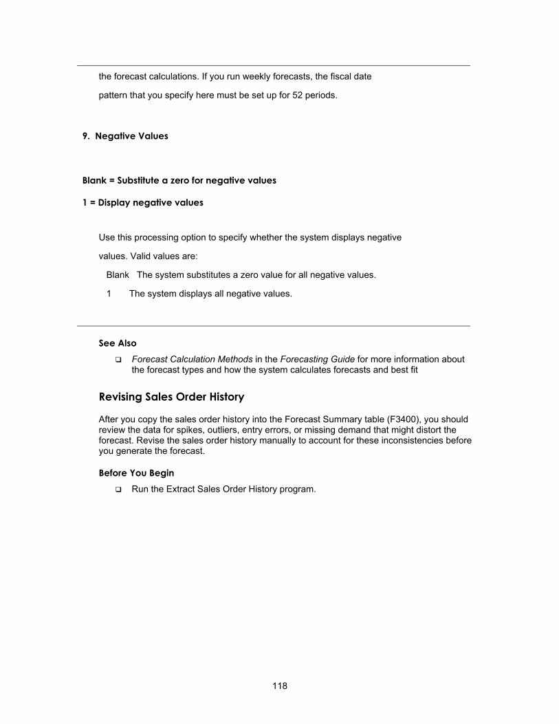
the forecast calculations. If you run weekly forecasts, the fiscal date
pattern that you specify here must be set up for 52 periods.
9. Negative Values
Blank = Substitute a zero for negative values
1 = Display negative values
Use this processing option to specify whether the system displays negative
values. Valid values are:
Blank The system substitutes a zero value for all negative values.
1 The system displays all negative values.
See Also Forecast Calculation Methods in the Forecasting Guide for more information about
the forecast types and how the system calculates forecasts and best fit
Revising Sales Order History
After you copy the sales order history into the Forecast Summary table (F3400), you should review the data for spikes, outliers, entry errors, or missing demand that might distort the forecast. Revise the sales order history manually to account for these inconsistencies before you generate the forecast.
Before You Begin Run the Extract Sales Order History program.
118
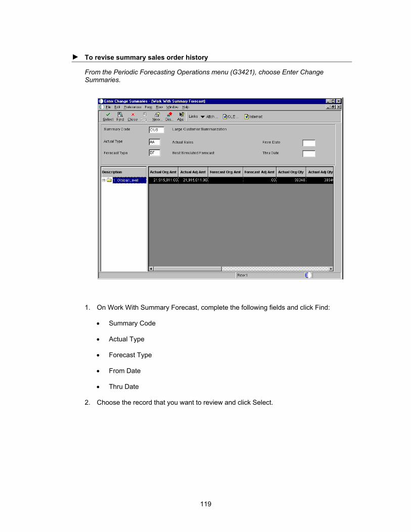
► To revise summary sales order history
From the Periodic Forecasting Operations menu (G3421), choose Enter Change Summaries.
1. On Work With Summary Forecast, complete the following fields and click Find:
• Summary Code
• Actual Type
• Forecast Type
• From Date
• Thru Date
2. Choose the record that you want to review and click Select.
119
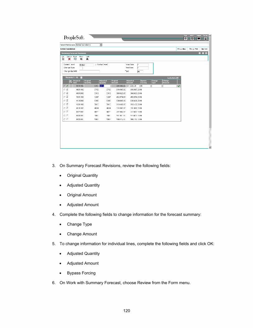
3. On Summary Forecast Revisions, review the following fields:
• Original Quantity
• Adjusted Quantity
• Original Amount
• Adjusted Amount
4. Complete the following fields to change information for the forecast summary:
• Change Type
• Change Amount
5. To change information for individual lines, complete the following fields and click OK:
• Adjusted Quantity
• Adjusted Amount
• Bypass Forcing
6. On Work with Summary Forecast, choose Review from the Form menu.
120
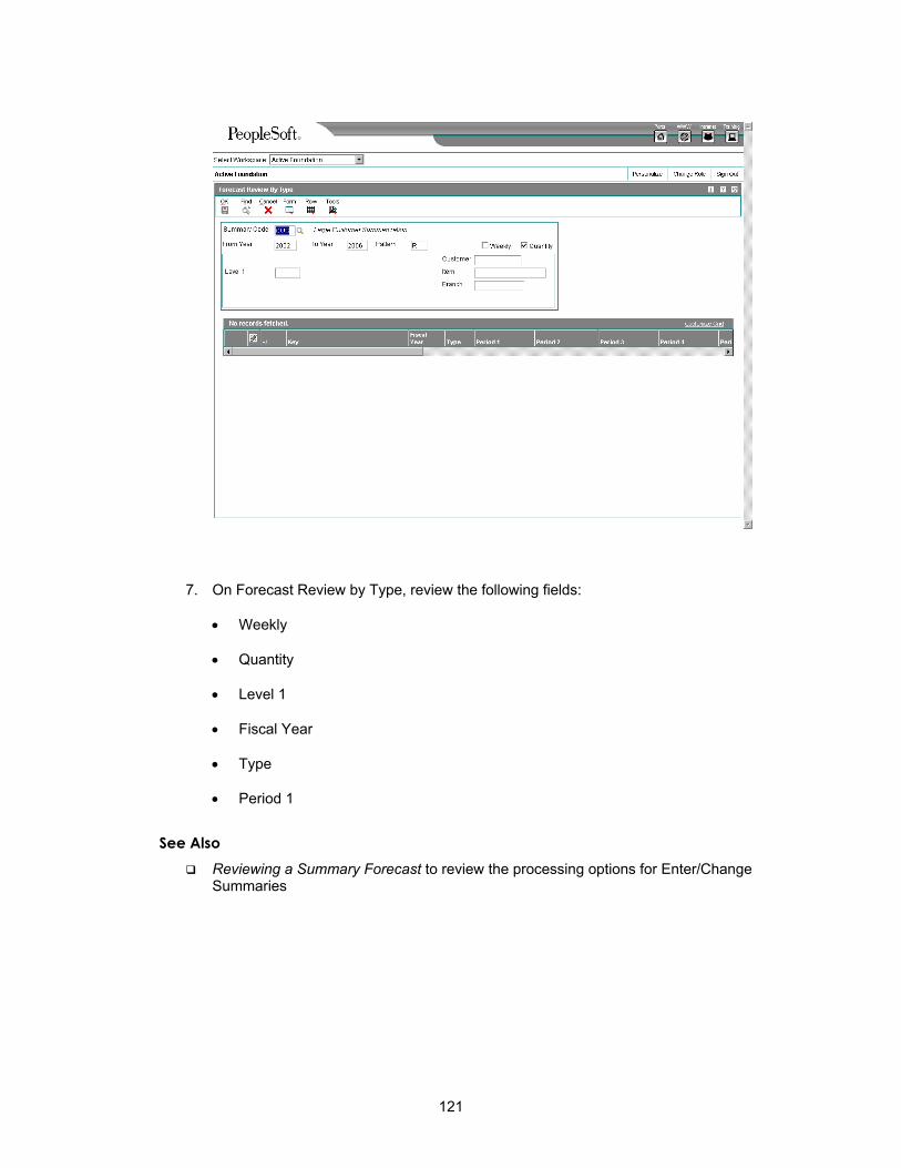
7. On Forecast Review by Type, review the following fields:
• Weekly
• Quantity
• Level 1
• Fiscal Year
• Type
• Period 1
See Also Reviewing a Summary Forecast to review the processing options for Enter/Change
Summaries
121
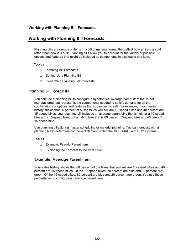
Working with Planning Bill Forecasts
Working with Planning Bill Forecasts
Planning bills are groups of items in a bill of material format that reflect how an item is sold rather than how it is built. Planning bills allow you to account for the variety of possible options and features that might be included as components in a saleable end item.
Topics Planning Bill Forecasts
Setting Up a Planning Bill
Generating Planning Bill Forecasts
Planning Bill Forecasts
You can use a planning bill to configure a hypothetical average parent item that is not manufactured, but represents the components needed to satisfy demand for all the combinations of options and features that you expect to sell. For example, if your sales history shows that 60 percent of all the bikes you sell are 10-speed bikes and 40 percent are 15-speed bikes, your planning bill includes an average parent bike that is neither a 10-speed bike nor a 15-speed bike, but a hybrid bike that is 60 percent 10-speed bike and 40 percent 15-speed bike.
Use planning bills during master scheduling or material planning. You can forecast with a planning bill to determine component demand within the MPS, MRP, and DRP systems.
Topics Example: Pseudo Parent Item
Exploding the Forecast to the Item Level
Example: Average Parent Item
Your sales history shows that 60 percent of the bikes that you sell are 10-speed bikes and 40 percent are 15-speed bikes. Of the 10-speed bikes, 70 percent are blue and 30 percent are green. Of the 15-speed bikes, 80 percent are blue and 20 percent are green. You use these percentages to configure an average parent item.
122
The average parent bike will be:
• 60 percent 10-speed
• 40 percent 15-speed
• 42 percent blue 10-speed (70 percent of 60 percent)
• 18 percent green 10-speed (30 percent of 60 percent)
• 32 percent blue 15-speed (80 percent of 40 percent)
• 8 percent green 15-speed (20 percent of 40 percent)
You decide to manufacture or purchase at these percentages.
Summary forecasts are more accurate than detail forecasts. For example, a forecast for the total number of bikes that will sell in 1998 is more accurate than a forecast for blue 10-speed bikes that will sell in 1998.
The forecast is based upon total bike sales history. This is the summary forecast. The option percentages produce a production (or purchase) forecast for each of the options. This is the detail forecast.
Exploding the Forecast to the Item Level
You use the planning bill to explode a forecast for the total number of products down to the level of the specific combination of options and features included in each saleable end item.
As you set up a planning bill, you designate each level of the item hierarchy above the end item level as an average parent with a planning code of 4. You designate the saleable end items as components of the phantom parents with a planning code of 5.
As you generate the planning bill forecast, you use processing options to designate a forecast type to be read as input and a forecast type to be calculated for the components. You also designate the calculated forecast type as the second type to be read so that it can
123
be exploded down through each level of the hierarchy until the forecast is applied to the saleable end items.
Example: Exploding the Forecast
You use a planning bill to configure an average parent item that represents total bike sales. This average parent bike represents the top level of the item hierarchy and is configured as follows:
• 60 percent 10-speed bike
• 40 percent 15-speed bike
Because bikes with both the 10-speed and 15-speed options can be further divided into blue and green bikes, both the total of all 10-speed bikes and the total of all 15-speed bikes are represented by average parent bikes on the second level of the item hierarchy. These average parents are configured as follows:
• 10-speed bikes:
• 70 percent blue
• 30 percent green
• 15-speed bikes:
• 80 percent blue
• 20 percent green
The system enables you to process multiple parent items as in this example. You use planning code 4 to designate each of the phantom products on the two higher levels of the hierarchy (total bikes on the top level and total 10-speed bikes and total 15-speed bikes on the second level) as parent items. You use planning code 5 to designate the end item bikes (for example, blue 15-speed bikes) on the bottom level as components of the phantom parent items.
You assign user defined codes to additional forecast types you want to include in the processing options that were not supplied with the system. For this forecast, you plan to use forecast types you have defined and assigned to codes 13 and 16. You designate 16 in processing options as the forecast type to be read as input for the top-level parent item and 13 as the forecast type to be created for calculating the forecast for the components.
The system reads the forecast for total bike sales determined by forecast type 16 and assigns a percentage of the total forecast to each of the portions of the total on the next level of the hierarchy (total 10-speed and total 15-speed sales).
These percentages are based on feature planned percents. Feature planned percents are the percentage of total products that include features that differentiate some products in the total from others. You define the feature planned percent on the Enter/Change Bill form. In this example, the feature planned percents are 60 percent for the 10-speed feature and 40 percent for the 15-speed feature.
The system then calculates a forecast based on forecast type 13 that it applies to the next level. You also designate 13 as the second forecast type to be read as input so the system reads the forecast for the second level, which it then applies to the saleable end items (blue and green 10-speed bikes and blue and green 15-speed bikes).
The system reads forecast type 16 and calculates a type 13 forecast of 20,000 total bikes. The system then reads the forecast and explodes it down the hierarchy to the end item level as follows:
124
• 60 percent of the 20,000 total bikes = 12,000 10-speed bikes
• 40 percent of the 20,000 total bikes = 8,000 15-speed bikes
• 70 percent of the 12,000 10-speed bikes (42 percent of total bike sales) = 8,400 blue 10-speed bikes
• 30 percent of the 12,000 10-speed bikes (18 percent of total bike sales) = 3,600 green 10-speed bikes
• 80 percent of the 8,000 15-speed bikes (32 percent of total bike sales) = 6,400 blue 15-speed bikes
• 20 percent of the 8,000 15-speed bikes (8 percent of total bike sales) = 1,600 green 15-speed bikes
See Also Working with Multi-Level Master Schedules in the Manufacturing and Distribution
Planning Guide
Setting Up a Planning Bill
You must set up a planning bill before you generate a planning bill forecast. You use the Product Data Management system to set up a planning bill. Then the system uses the planning bill to generate a forecast for the hypothetical average parent item. The forecast shows the component level exploded.
Topics Setting up item master information
Entering planning bills
Setting Up Item Master Information
Before you enter the criteria that you want to use on the planning bill, you must set up item master information on which the planning is based. The system stores this information in the Item Master table (F4101).
The Item Branch table (F4102) also stores the item information. After you add item master records for appropriate part numbers, the system retrieves item information from the Item Branch table.
► To set up item master information
From the Inventory Master/Transactions menu (G4111), choose Item Master.
125
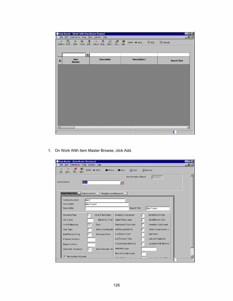
1. On Work With Item Master Browse, click Add.
126
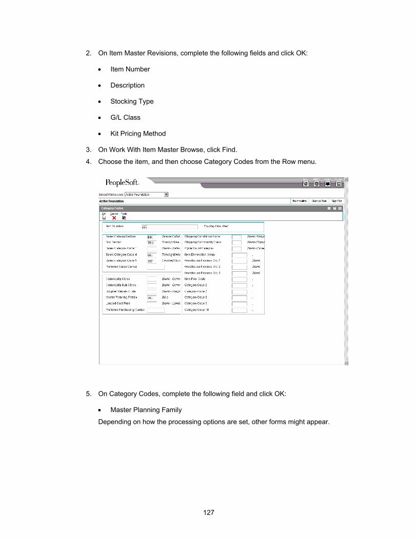
2. On Item Master Revisions, complete the following fields and click OK:
• Item Number
• Description
• Stocking Type
• G/L Class
• Kit Pricing Method
3. On Work With Item Master Browse, click Find.
4. Choose the item, and then choose Category Codes from the Row menu.
5. On Category Codes, complete the following field and click OK:
• Master Planning Family
Depending on how the processing options are set, other forms might appear.
127
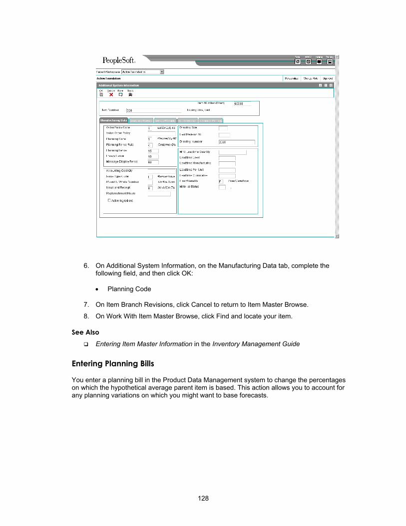
6. On Additional System Information, on the Manufacturing Data tab, complete the following field, and then click OK:
• Planning Code
7. On Item Branch Revisions, click Cancel to return to Item Master Browse.
8. On Work With Item Master Browse, click Find and locate your item.
See Also Entering Item Master Information in the Inventory Management Guide
Entering Planning Bills
You enter a planning bill in the Product Data Management system to change the percentages on which the hypothetical average parent item is based. This action allows you to account for any planning variations on which you might want to base forecasts.
128

► To enter planning bills
From the Daily PDM Discrete menu (G3011), choose Enter/Change Bill.
1. On Work with Bill of Material, complete the following fields and click Find:
• Item Number
• Branch/Plant
2. Choose the item number and click Select.
129
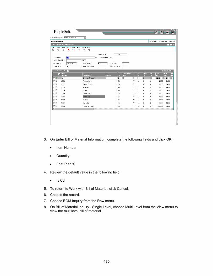
3. On Enter Bill of Material Information, complete the following fields and click OK:
• Item Number
• Quantity
• Feat Plan %
4. Review the default value in the following field:
• Is Cd
5. To return to Work with Bill of Material, click Cancel.
6. Choose the record.
7. Choose BOM Inquiry from the Row menu.
8. On Bill of Material Inquiry - Single Level, choose Multi Level from the View menu to view the multilevel bill of material.
130
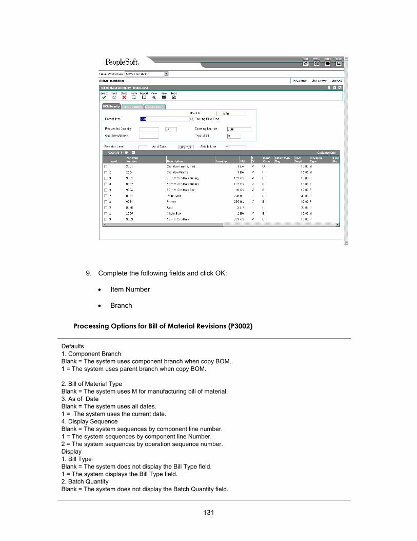
9. Complete the following fields and click OK:
• Item Number
• Branch
Processing Options for Bill of Material Revisions (P3002)
Defaults 1. Component Branch Blank = The system uses component branch when copy BOM. 1 = The system uses parent branch when copy BOM. 2. Bill of Material Type Blank = The system uses M for manufacturing bill of material. 3. As of Date Blank = The system uses all dates. 1 = The system uses the current date. 4. Display Sequence Blank = The system sequences by component line number. 1 = The system sequences by component line Number. 2 = The system sequences by operation sequence number. Display 1. Bill Type Blank = The system does not display the Bill Type field. 1 = The system displays the Bill Type field. 2. Batch Quantity Blank = The system does not display the Batch Quantity field.
131
1 = The system displays the Batch Quantity field. Versions Enter the version for each program. If left blank, version ZJDE0001 will be used. 1. Single Level BOM Print (R30460) 2. Multi Level BOM Print (R30460) 3. ECO Workbench (P30225) 4. Component Maintenance (P3015) 5. ECO Header [P30BREV] 6. Bill of Material Where Used (P30201) 7. Item Master (P4101B) 8. Co/By- Products Inquiry (P30211) 9. Bill of Material Inquiry (P30200) Edit 1. Item Branch Validation Blank = The system does not check to see if the item branch is valid. 1 = The system checks for a valid item branch record. Interop 1. Transaction Type Blank = The system does not perform outbound interoperability processing. JDEBOM = The system performs outbound interoperability processing. 2. Write Image for a Change Transaction Blank = The system stores the after image from F3002 to F3002Z1 1 = The system stores the before image from F3002 to F3002Z1 3. Interoperability Outbound (R00460) Blank = Ths system uses the ZJDE0001 version of R00460.
Generating Planning Bill Forecasts
From the Single Site Periodic Planning Operations menu (G3422), choose DRP Regeneration.
After setting up a planning bill, you can generate a planning bill forecast to help you plan configurations for end products. The material planning generation program reads the detail forecast for the selected parent planning bill items and explodes it to create a forecast for the planning bill components for the same time periods.
Before You Begin Enter a planning bill. See Entering Planning Bills.
Run Enter/Change Forecast manually to add the forecast for the parent item.
Processing Options for MRP/MPS Requirements Planning (R3482)
Horizon 1. Generation Start Date 2. Past Due Periods 0 (default) 1 2 3. Planning Horizon Periods Number of planning days Number of planning weeks Number of planning months Parameters 1. Generation Mode 1 = net change
132
2 = gross regeneration 2. Generation Type 1 = single level MPS/DRP 2 = planning bill 3 = multi-level MPS 4 = MRP with or without MPS 5 = MRP with frozen MPS 6 = Initialize Order Promising Engine 3. UDC Type 4. Version of Supply/Demand Inclusion Rules On Hand Data 1. Include Lot Expiration Dates blank = do not include 1 = include 2. Safety Stock Decrease blank = do not decrease 1 = decrease 3. Receipt Routing Quantities Quantity in Transit blank = do not include in on-hand inventory 1 = include in on-hand inventory Quantity in Inspection blank = do not include in on-hand inventory 1 = include in on-hand inventory User Defined Quantity 1 blank = do not include in on-hand inventory 1 = include in on-hand inventory User Defined Quantity 2 blank = do not include in on-hand inventory 1 = include in on-hand inventory 4. Lot Hold Codes (up to 5) blank = inlclude no held lots in calculation of on-hand inventory * = include all held lots in calculation of on-hand inventory Forecasting 1. Forecast Types Used ( up to 5 ) 2. MPS Forecast Type For Planning Bills 3. Forecast Consumption Logic blank = do not use forecast consumption 1 = use forecast consumption Document Types 1. Purchase Orders 2. Work Orders 3. Rate Schedules Lead Times 1. Purchased Item Safety Leadtime 2. Manufactured Item Safety Leadtime 3. Expedite Damper Days 4. Defer Damper Days Performance 1. Clear F3411/F3412/F3413 Tables
133
blank = do not clear tables 1 = clear tables 2. Initialize MPS/MRP Print Code. blank = do not initialize the Item Branch file 1 = initialize the Item Branch file 3. Messages And Time Series For Phantom Items blank = do not generate 1 = generate 4. Ending Work Order Status blank = all messages exploded 5. Extend Rate Based Adjustments blank = do not extend 1 = extend 6. Closed Rate Status Process Mfg 1. Process Planning blank = discrete 1 = process Parallel 1. Number of Subsystem Jobs 0 = Default 2. Pre Processing blank = Do not perform pre processing 1= Perform pre processing
What You Should Know About Processing Options
Document Types Used in Planning
When you choose a forecast type to use with a planning bill, you must also enter the type code for this forecast as a forecast type to be read. This allows the system to read the forecast and explode it down to the component level. You can specify up to five forecast types to be read in a sequence that you specify.
134

Working With Forecasting Interoperability
To address the information requirements of an enterprise, companies sometimes use products from different software and hardware providers. Interoperability between different products is key to successfully implementing the enterprise solution. Full interoperability among different systems results in a flow of data between the different products that is seamless to the user. The OneWorld Interoperability function provides an interface that facilitates exchanging transactions with external systems. These transactions include both inbound and outbound.
External systems send information to the interface tables, using either an external program or flat files and the Inbound Flat File Conversion program. The sending party is responsible for conforming to format and other requirements for the interface tables.
You run a transaction process (a batch program) that validates the data, updates valid data to the J.D. Edwards application tables, and sends action messages to the Employee Work Center about any invalid data.
You use an inquiry function to interactively review the data for correctness, and then run the transaction process again. You can repeat this process if necessary.
You set a processing option to specify the transaction type for the outbound transaction. The system uses the master business function for the type of transaction, creates a copy of the transaction, and places the copy in the interface table where external systems can access it.
You use the purge function to remove obsolete and unnecessary data from interface tables. Your system is more efficient when you keep these tables as small as possible.
135
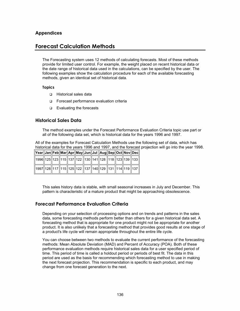
Appendices
Forecast Calculation Methods
The Forecasting system uses 12 methods of calculating forecasts. Most of these methods provide for limited user control. For example, the weight placed on recent historical data or the date range of historical data used in the calculations, can be specified by the user. The following examples show the calculation procedure for each of the available forecasting methods, given an identical set of historical data.
Topics Historical sales data
Forecast performance evaluation criteria
Evaluating the forecasts
Historical Sales Data
The method examples under the Forecast Performance Evaluation Criteria topic use part or all of the following data set, which is historical data for the years 1996 and 1997.
All of the examples for Forecast Calculation Methods use the following set of data, which has historical data for the years 1996 and 1997, and the forecast projection will go into the year 1998. Year Jan Feb Mar Apr May Jun Jul Aug Sep Oct Nov Dec
1996 125 123 115 137 122 130 141 128 118 123 139 133
1997 128 117 115 125 122 137 140 129 131 114 119 137
This sales history data is stable, with small seasonal increases in July and December. This pattern is characteristic of a mature product that might be approaching obsolescence.
Forecast Performance Evaluation Criteria
Depending on your selection of processing options and on trends and patterns in the sales data, some forecasting methods perform better than others for a given historical data set. A forecasting method that is appropriate for one product might not be appropriate for another product. It is also unlikely that a forecasting method that provides good results at one stage of a product's life cycle will remain appropriate throughout the entire life cycle.
You can choose between two methods to evaluate the current performance of the forecasting methods: Mean Absolute Deviation (MAD) and Percent of Accuracy (POA). Both of these performance evaluation methods require historical sales data for a user specified period of time. This period of time is called a holdout period or periods of best fit. The data in this period are used as the basis for recommending which forecasting method to use in making the next forecast projection. This recommendation is specific to each product, and may change from one forecast generation to the next.
136
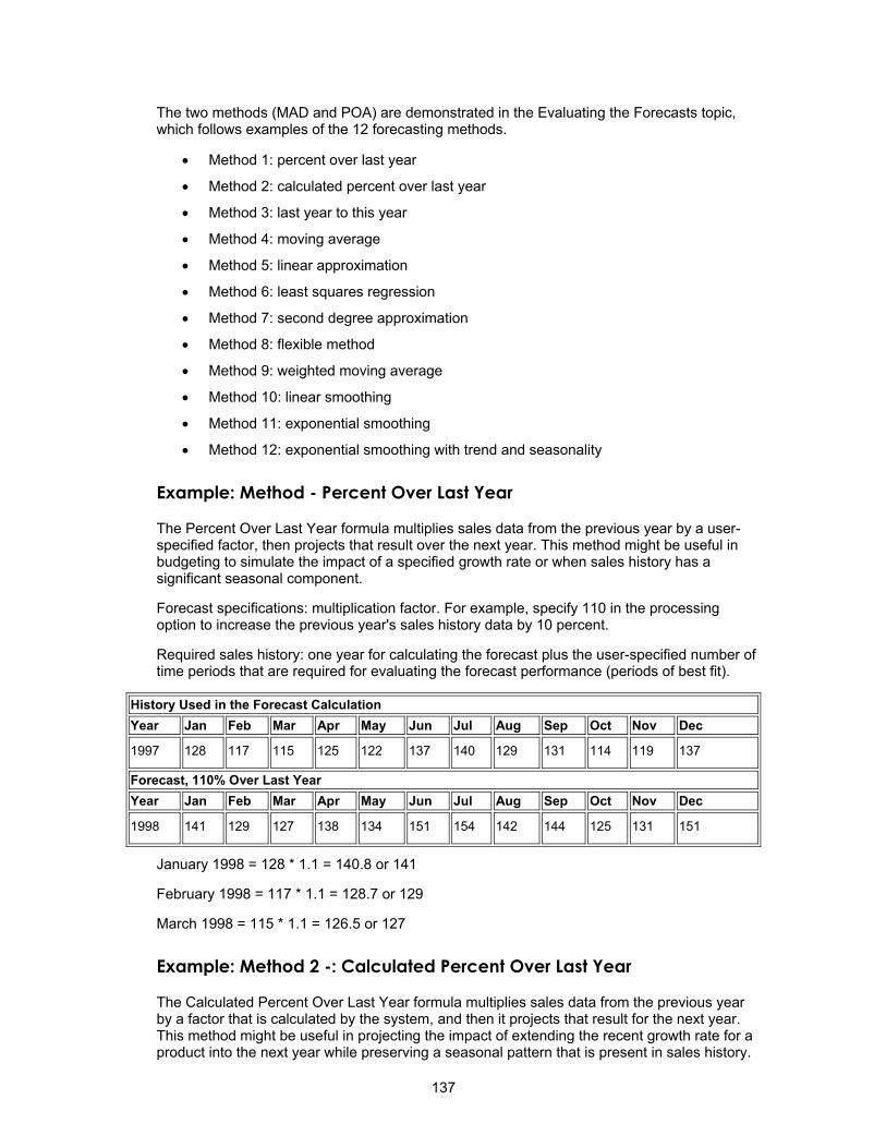
The two methods (MAD and POA) are demonstrated in the Evaluating the Forecasts topic, which follows examples of the 12 forecasting methods.
• Method 1: percent over last year
• Method 2: calculated percent over last year
• Method 3: last year to this year
• Method 4: moving average
• Method 5: linear approximation
• Method 6: least squares regression
• Method 7: second degree approximation
• Method 8: flexible method
• Method 9: weighted moving average
• Method 10: linear smoothing
• Method 11: exponential smoothing
• Method 12: exponential smoothing with trend and seasonality
Example: Method - Percent Over Last Year
The Percent Over Last Year formula multiplies sales data from the previous year by a user-specified factor, then projects that result over the next year. This method might be useful in budgeting to simulate the impact of a specified growth rate or when sales history has a significant seasonal component.
Forecast specifications: multiplication factor. For example, specify 110 in the processing option to increase the previous year's sales history data by 10 percent.
Required sales history: one year for calculating the forecast plus the user-specified number of time periods that are required for evaluating the forecast performance (periods of best fit).
History Used in the Forecast Calculation Year Jan Feb Mar Apr May Jun Jul Aug Sep Oct Nov Dec
1997 128 117 115 125 122 137 140 129 131 114 119 137
Forecast, 110% Over Last Year Year Jan Feb Mar Apr May Jun Jul Aug Sep Oct Nov Dec
1998 141 129 127 138 134 151 154 142 144 125 131 151
January 1998 = 128 * 1.1 = 140.8 or 141
February 1998 = 117 * 1.1 = 128.7 or 129
March 1998 = 115 * 1.1 = 126.5 or 127
Example: Method 2 -: Calculated Percent Over Last Year
The Calculated Percent Over Last Year formula multiplies sales data from the previous year by a factor that is calculated by the system, and then it projects that result for the next year. This method might be useful in projecting the impact of extending the recent growth rate for a product into the next year while preserving a seasonal pattern that is present in sales history.
137
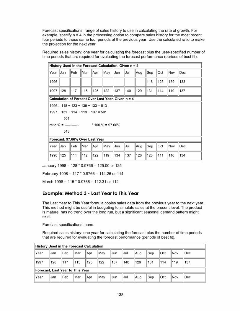
Forecast specifications: range of sales history to use in calculating the rate of growth. For example, specify n = 4 in the processing option to compare sales history for the most recent four periods to those same four periods of the previous year. Use the calculated ratio to make the projection for the next year.
Required sales history: one year for calculating the forecast plus the user-specified number of time periods that are required for evaluating the forecast performance (periods of best fit).
History Used in the Forecast Calculation, Given n = 4
Year Jan Feb Mar Apr May Jun Jul Aug Sep Oct Nov Dec
1996 118 123 139 133
1997 128 117 115 125 122 137 140 129 131 114 119 137
Calculation of Percent Over Last Year, Given n = 4
1996... 118 + 123 + 139 + 133 = 513
1997... 131 + 114 + 119 + 137 = 501
501
ratio % = ------------ * 100 % = 97.66%
513
Forecast, 97.66% Over Last Year
Year Jan Feb Mar Apr May Jun Jul Aug Sep Oct Nov Dec
1998 125 114 112 122 119 134 137 126 128 111 116 134
January 1998 = 128 * 0.9766 = 125.00 or 125
February 1998 = 117 * 0.9766 = 114.26 or 114
March 1998 = 115 * 0.9766 = 112.31 or 112
Example: Method 3 - Last Year to This Year
The Last Year to This Year formula copies sales data from the previous year to the next year. This method might be useful in budgeting to simulate sales at the present level. The product is mature, has no trend over the long run, but a significant seasonal demand pattern might exist.
Forecast specifications: none.
Required sales history: one year for calculating the forecast plus the number of time periods that are required for evaluating the forecast performance (periods of best fit).
History Used in the Forecast Calculation
Year Jan Feb Mar Apr May Jun Jul Aug Sep Oct Nov Dec
1997 128 117 115 125 122 137 140 129 131 114 119 137
Forecast, Last Year to This Year
Year Jan Feb Mar Apr May Jun Jul Aug Sep Oct Nov Dec
138
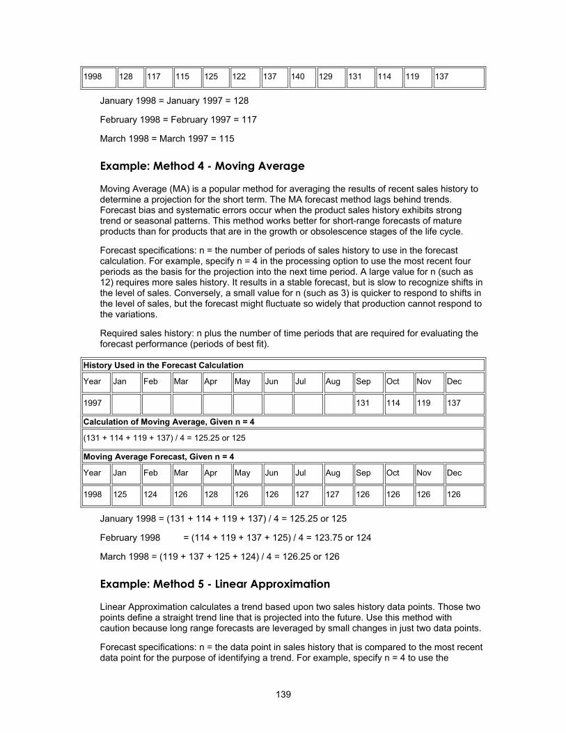
1998 128 117 115 125 122 137 140 129 131 114 119 137
January 1998 = January 1997 = 128
February 1998 = February 1997 = 117
March 1998 = March 1997 = 115
Example: Method 4 - Moving Average
Moving Average (MA) is a popular method for averaging the results of recent sales history to determine a projection for the short term. The MA forecast method lags behind trends. Forecast bias and systematic errors occur when the product sales history exhibits strong trend or seasonal patterns. This method works better for short-range forecasts of mature products than for products that are in the growth or obsolescence stages of the life cycle.
Forecast specifications: n = the number of periods of sales history to use in the forecast calculation. For example, specify n = 4 in the processing option to use the most recent four periods as the basis for the projection into the next time period. A large value for n (such as 12) requires more sales history. It results in a stable forecast, but is slow to recognize shifts in the level of sales. Conversely, a small value for n (such as 3) is quicker to respond to shifts in the level of sales, but the forecast might fluctuate so widely that production cannot respond to the variations.
Required sales history: n plus the number of time periods that are required for evaluating the forecast performance (periods of best fit).
History Used in the Forecast Calculation
Year Jan Feb Mar Apr May Jun Jul Aug Sep Oct Nov Dec
1997 131 114 119 137
Calculation of Moving Average, Given n = 4
(131 + 114 + 119 + 137) / 4 = 125.25 or 125
Moving Average Forecast, Given n = 4
Year Jan Feb Mar Apr May Jun Jul Aug Sep Oct Nov Dec
1998 125 124 126 128 126 126 127 127 126 126 126 126
January 1998 = (131 + 114 + 119 + 137) / 4 = 125.25 or 125
February 1998 = (114 + 119 + 137 + 125) / 4 = 123.75 or 124
March 1998 = (119 + 137 + 125 + 124) / 4 = 126.25 or 126
Example: Method 5 - Linear Approximation
Linear Approximation calculates a trend based upon two sales history data points. Those two points define a straight trend line that is projected into the future. Use this method with caution because long range forecasts are leveraged by small changes in just two data points.
Forecast specifications: n = the data point in sales history that is compared to the most recent data point for the purpose of identifying a trend. For example, specify n = 4 to use the
139
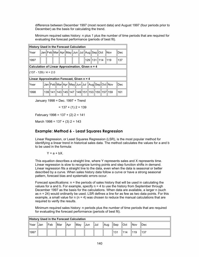
difference between December 1997 (most recent data) and August 1997 (four periods prior to December) as the basis for calculating the trend.
Minimum required sales history: n plus 1 plus the number of time periods that are required for evaluating the forecast performance (periods of best fit).
History Used in the Forecast Calculation
Year Jan Feb Mar Apr May Jun Jul Aug Sep Oct Nov Dec
1997 129 131 114 119 137
Calculation of Linear Approximation, Given n = 4
(137 - 129) / 4 = 2.0
Linear Approximation Forecast, Given n = 4
Year Jan Feb Mar Apr May Jun Jul Aug Sep Oct Nov Dec
1998 139 141 143 145 147 149 151 153 155 157 159 161
January 1998 = Dec. 1997 + Trend
= 137 + (1) 2 = 139
February 1998 = 137 + (2) 2 = 141
March 1998 = 137 + (3) 2 = 143
Example: Method 6 - Least Squares Regression
Linear Regression, or Least Squares Regression (LSR), is the most popular method for identifying a linear trend in historical sales data. The method calculates the values for a and b to be used in the formula:
Y = a + bX.
This equation describes a straight line, where Y represents sales and X represents time. Linear regression is slow to recognize turning points and step function shifts in demand. Linear regression fits a straight line to the data, even when the data is seasonal or better described by a curve. When sales history data follow a curve or have a strong seasonal pattern, forecast bias and systematic errors occur.
Forecast specifications: n = the periods of sales history that will be used in calculating the values for a and b. For example, specify n = 4 to use the history from September through December 1997 as the basis for the calculations. When data are available, a larger n (such as n = 24) would ordinarily be used. LSR defines a line for as few as two data points. For this example, a small value for n (n = 4) was chosen to reduce the manual calculations that are required to verify the results.
Minimum required sales history: n periods plus the number of time periods that are required for evaluating the forecast performance (periods of best fit).
History Used in the Forecast Calculation
Year Jan Feb Mar Apr May Jun Jul Aug Sep Oct Nov Dec
1997 131 114 119 137
140
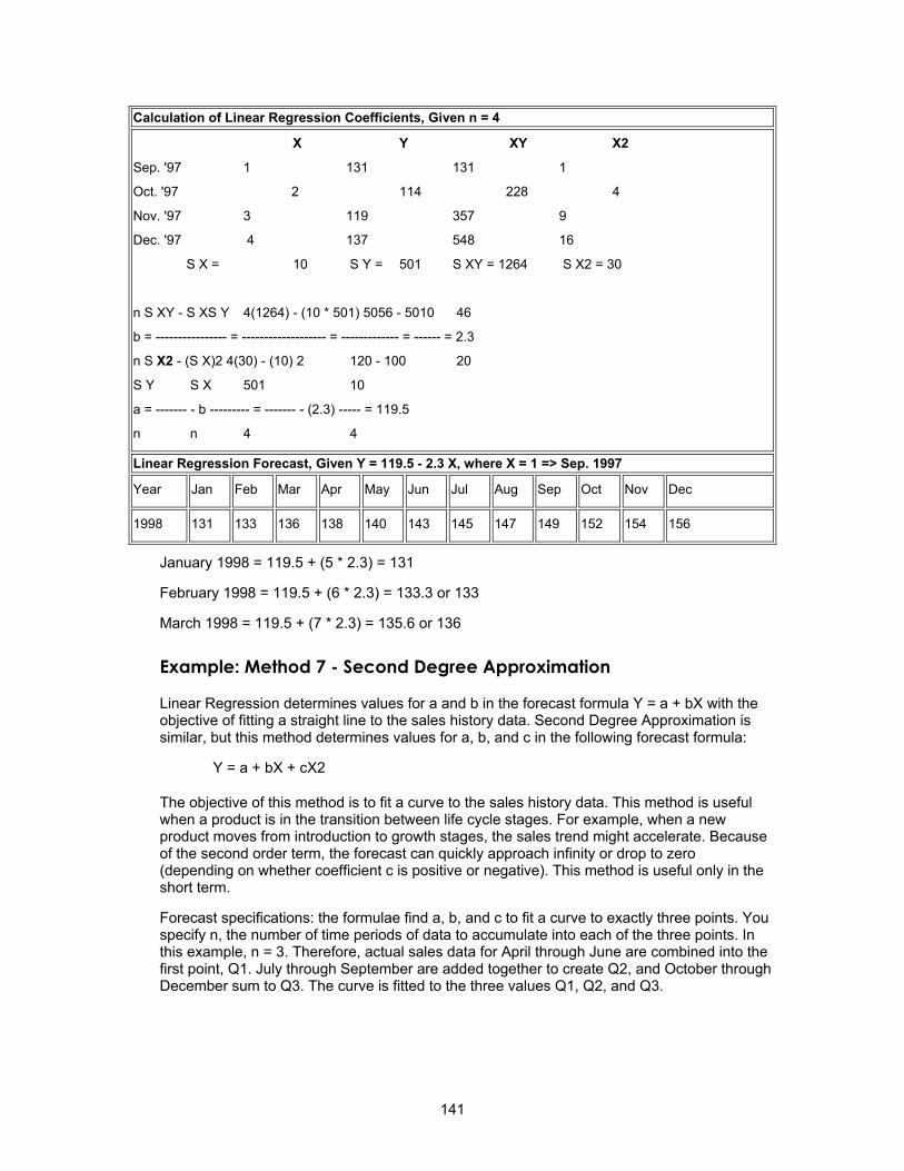
Calculation of Linear Regression Coefficients, Given n = 4
X Y XY X2
Sep. '97 1 131 131 1
Oct. '97 2 114 228 4
Nov. '97 3 119 357 9
Dec. '97 4 137 548 16
S X = 10 S Y = 501 S XY = 1264 S X2 = 30
n S XY - S XS Y 4(1264) - (10 * 501) 5056 - 5010 46
b = ---------------- = ------------------- = ------------- = ------ = 2.3
n S X2 - (S X)2 4(30) - (10) 2 120 - 100 20
S Y S X 501 10
a = ------- - b --------- = ------- - (2.3) ----- = 119.5
n n 4 4
Linear Regression Forecast, Given Y = 119.5 - 2.3 X, where X = 1 => Sep. 1997
Year Jan Feb Mar Apr May Jun Jul Aug Sep Oct Nov Dec
1998 131 133 136 138 140 143 145 147 149 152 154 156
January 1998 = 119.5 + (5 * 2.3) = 131
February 1998 = 119.5 + (6 * 2.3) = 133.3 or 133
March 1998 = 119.5 + (7 * 2.3) = 135.6 or 136
Example: Method 7 - Second Degree Approximation
Linear Regression determines values for a and b in the forecast formula Y = a + bX with the objective of fitting a straight line to the sales history data. Second Degree Approximation is similar, but this method determines values for a, b, and c in the following forecast formula:
Y = a + bX + cX2
The objective of this method is to fit a curve to the sales history data. This method is useful when a product is in the transition between life cycle stages. For example, when a new product moves from introduction to growth stages, the sales trend might accelerate. Because of the second order term, the forecast can quickly approach infinity or drop to zero (depending on whether coefficient c is positive or negative). This method is useful only in the short term.
Forecast specifications: the formulae find a, b, and c to fit a curve to exactly three points. You specify n, the number of time periods of data to accumulate into each of the three points. In this example, n = 3. Therefore, actual sales data for April through June are combined into the first point, Q1. July through September are added together to create Q2, and October through December sum to Q3. The curve is fitted to the three values Q1, Q2, and Q3.
141
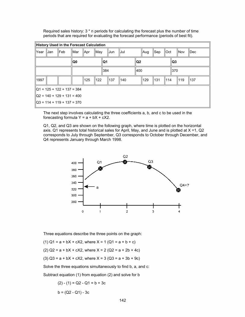
Required sales history: 3 * n periods for calculating the forecast plus the number of time periods that are required for evaluating the forecast performance (periods of best fit).
History Used in the Forecast Calculation
Year Jan Feb Mar Apr May Jun Jul Aug Sep Oct Nov Dec
Q0 Q1 Q2 Q3
384 400 370
1997 125 122 137 140 129 131 114 119 137
Q1 = 125 + 122 + 137 = 384
Q2 = 140 + 129 + 131 = 400
Q3 = 114 + 119 + 137 = 370
The next step involves calculating the three coefficients a, b, and c to be used in the forecasting formula Y = a + bX + cX2.
Q1, Q2, and Q3 are shown on the following graph, where time is plotted on the horizontal axis. Q1 represents total historical sales for April, May, and June and is plotted at X =1, Q2 corresponds to July through September, Q3 corresponds to October through December, and Q4 represents January through March 1998.
Three equations describe the three points on the graph:
(1) Q1 = a + bX + cX2, where X = 1 (Q1 = a + b + c)
(2) Q2 = a + bX + cX2, where X = 2 (Q2 = a + 2b + 4c)
(3) Q3 = a + bX + cX2, where X = 3 (Q3 = a + 3b + 9c)
Solve the three equations simultaneously to find b, a, and c:
Subtract equation (1) from equation (2) and solve for b
(2) - (1) = Q2 - Q1 = b + 3c
b = (Q2 - Q1) - 3c
142
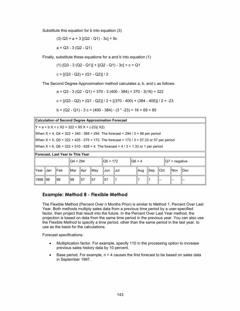
Substitute this equation for b into equation (3)
(3) Q3 = a + 3 [(Q2 - Q1) - 3c] + 9c
a = Q3 - 3 (Q2 - Q1)
Finally, substitute these equations for a and b into equation (1)
(1) [Q3 - 3 (Q2 - Q1)] + [(Q2 - Q1) - 3c] + c = Q1
c = [(Q3 - Q2) + (Q1 - Q2)] / 2
The Second Degree Approximation method calculates a, b, and c as follows:
a = Q3 - 3 (Q2 - Q1) = 370 - 3 (400 - 384) = 370 - 3(16) = 322
c = [(Q3 - Q2) + (Q1 - Q2)] / 2 = [(370 - 400) + (384 - 400)] / 2 = -23
b = (Q2 - Q1) - 3 c = (400 - 384) - (3 * -23) = 16 + 69 = 85
Calculation of Second Degree Approximation Forecast
Y = a + b X + c X2 = 322 + 85 X + (-23)( X2)
When X = 4, Q4 = 322 + 340 - 368 = 294. The forecast = 294 / 3 = 98 per period
When X = 5, Q5 = 322 + 425 - 575 = 172. The forecast = 172 / 3 = 57.33 or 57 per period
When X = 6, Q6 = 322 + 510 - 828 = 4. The forecast = 4 / 3 = 1.33 or 1 per period
Forecast, Last Year to This Year
Q4 = 294 Q5 = 172 Q6 = 4 Q7 = negative
Year Jan Feb Mar Apr May Jun Jul Aug Sep Oct Nov Dec
1998 98 98 98 57 57 57 1 1 1 -- -- --
Example: Method 8 - Flexible Method
The Flexible Method (Percent Over n Months Prior) is similar to Method 1, Percent Over Last Year. Both methods multiply sales data from a previous time period by a user-specified factor, then project that result into the future. In the Percent Over Last Year method, the projection is based on data from the same time period in the previous year. You can also use the Flexible Method to specify a time period, other than the same period in the last year, to use as the basis for the calculations.
Forecast specifications:
• Multiplication factor. For example, specify 110 in the processing option to increase previous sales history data by 10 percent.
• Base period. For example, n = 4 causes the first forecast to be based on sales data in September 1997.
143
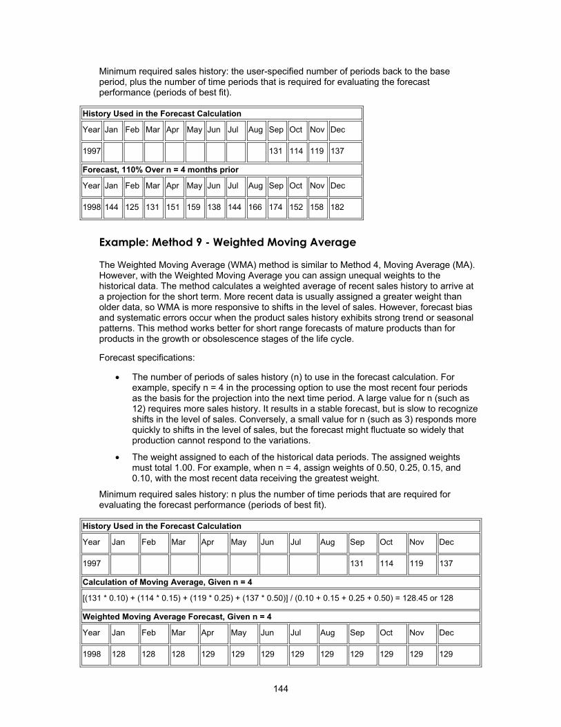
Minimum required sales history: the user-specified number of periods back to the base period, plus the number of time periods that is required for evaluating the forecast performance (periods of best fit).
History Used in the Forecast Calculation
Year Jan Feb Mar Apr May Jun Jul Aug Sep Oct Nov Dec
1997 131 114 119 137
Forecast, 110% Over n = 4 months prior
Year Jan Feb Mar Apr May Jun Jul Aug Sep Oct Nov Dec
1998 144 125 131 151 159 138 144 166 174 152 158 182
Example: Method 9 - Weighted Moving Average
The Weighted Moving Average (WMA) method is similar to Method 4, Moving Average (MA). However, with the Weighted Moving Average you can assign unequal weights to the historical data. The method calculates a weighted average of recent sales history to arrive at a projection for the short term. More recent data is usually assigned a greater weight than older data, so WMA is more responsive to shifts in the level of sales. However, forecast bias and systematic errors occur when the product sales history exhibits strong trend or seasonal patterns. This method works better for short range forecasts of mature products than for products in the growth or obsolescence stages of the life cycle.
Forecast specifications:
• The number of periods of sales history (n) to use in the forecast calculation. For example, specify n = 4 in the processing option to use the most recent four periods as the basis for the projection into the next time period. A large value for n (such as 12) requires more sales history. It results in a stable forecast, but is slow to recognize shifts in the level of sales. Conversely, a small value for n (such as 3) responds more quickly to shifts in the level of sales, but the forecast might fluctuate so widely that production cannot respond to the variations.
• The weight assigned to each of the historical data periods. The assigned weights must total 1.00. For example, when n = 4, assign weights of 0.50, 0.25, 0.15, and 0.10, with the most recent data receiving the greatest weight.
Minimum required sales history: n plus the number of time periods that are required for evaluating the forecast performance (periods of best fit).
History Used in the Forecast Calculation
Year Jan Feb Mar Apr May Jun Jul Aug Sep Oct Nov Dec
1997 131 114 119 137
Calculation of Moving Average, Given n = 4
[(131 * 0.10) + (114 * 0.15) + (119 * 0.25) + (137 * 0.50)] / (0.10 + 0.15 + 0.25 + 0.50) = 128.45 or 128
Weighted Moving Average Forecast, Given n = 4
Year Jan Feb Mar Apr May Jun Jul Aug Sep Oct Nov Dec
1998 128 128 128 129 129 129 129 129 129 129 129 129
144
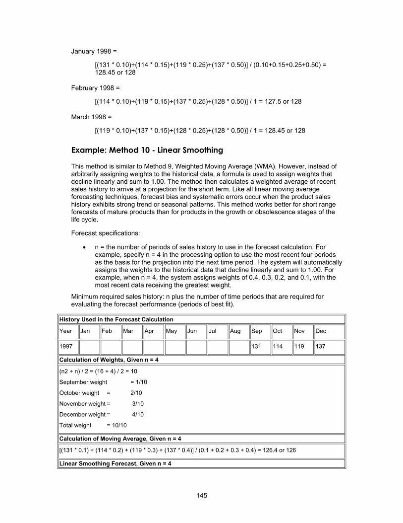
January 1998 =
[(131 * 0.10)+(114 * 0.15)+(119 * 0.25)+(137 * 0.50)] / (0.10+0.15+0.25+0.50) = 128.45 or 128
February 1998 =
[(114 * 0.10)+(119 * 0.15)+(137 * 0.25)+(128 * 0.50)] / 1 = 127.5 or 128
March 1998 =
[(119 * 0.10)+(137 * 0.15)+(128 * 0.25)+(128 * 0.50)] / 1 = 128.45 or 128
Example: Method 10 - Linear Smoothing
This method is similar to Method 9, Weighted Moving Average (WMA). However, instead of arbitrarily assigning weights to the historical data, a formula is used to assign weights that decline linearly and sum to 1.00. The method then calculates a weighted average of recent sales history to arrive at a projection for the short term. Like all linear moving average forecasting techniques, forecast bias and systematic errors occur when the product sales history exhibits strong trend or seasonal patterns. This method works better for short range forecasts of mature products than for products in the growth or obsolescence stages of the life cycle.
Forecast specifications:
• n = the number of periods of sales history to use in the forecast calculation. For example, specify n = 4 in the processing option to use the most recent four periods as the basis for the projection into the next time period. The system will automatically assigns the weights to the historical data that decline linearly and sum to 1.00. For example, when n = 4, the system assigns weights of 0.4, 0.3, 0.2, and 0.1, with the most recent data receiving the greatest weight.
Minimum required sales history: n plus the number of time periods that are required for evaluating the forecast performance (periods of best fit).
History Used in the Forecast Calculation
Year Jan Feb Mar Apr May Jun Jul Aug Sep Oct Nov Dec
1997 131 114 119 137
Calculation of Weights, Given n = 4
(n2 + n) / 2 = (16 + 4) / 2 = 10
September weight = 1/10
October weight = 2/10
November weight = 3/10
December weight = 4/10
Total weight = 10/10
Calculation of Moving Average, Given n = 4
[(131 * 0.1) + (114 * 0.2) + (119 * 0.3) + (137 * 0.4)] / (0.1 + 0.2 + 0.3 + 0.4) = 126.4 or 126
Linear Smoothing Forecast, Given n = 4
145
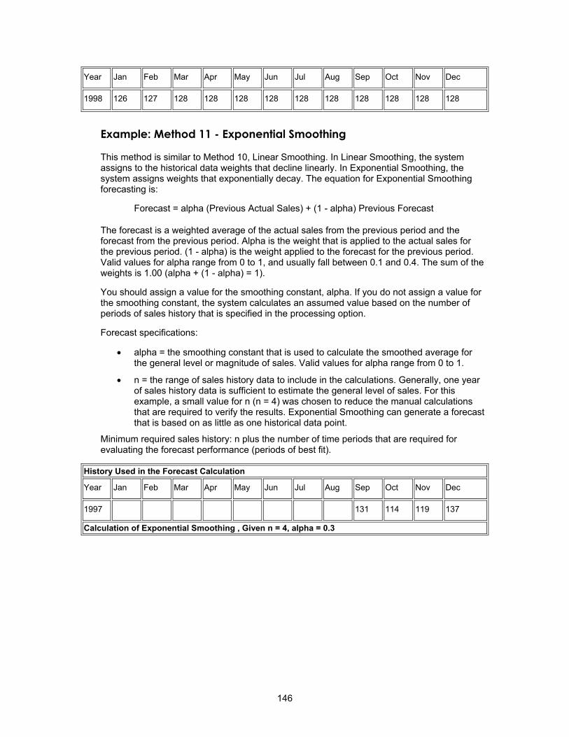
Year Jan Feb Mar Apr May Jun Jul Aug Sep Oct Nov Dec
1998 126 127 128 128 128 128 128 128 128 128 128 128
Example: Method 11 - Exponential Smoothing
This method is similar to Method 10, Linear Smoothing. In Linear Smoothing, the system assigns to the historical data weights that decline linearly. In Exponential Smoothing, the system assigns weights that exponentially decay. The equation for Exponential Smoothing forecasting is:
Forecast = alpha (Previous Actual Sales) + (1 - alpha) Previous Forecast
The forecast is a weighted average of the actual sales from the previous period and the forecast from the previous period. Alpha is the weight that is applied to the actual sales for the previous period. (1 - alpha) is the weight applied to the forecast for the previous period. Valid values for alpha range from 0 to 1, and usually fall between 0.1 and 0.4. The sum of the weights is 1.00 (alpha + (1 - alpha) = 1).
You should assign a value for the smoothing constant, alpha. If you do not assign a value for the smoothing constant, the system calculates an assumed value based on the number of periods of sales history that is specified in the processing option.
Forecast specifications:
• alpha = the smoothing constant that is used to calculate the smoothed average for the general level or magnitude of sales. Valid values for alpha range from 0 to 1.
• n = the range of sales history data to include in the calculations. Generally, one year of sales history data is sufficient to estimate the general level of sales. For this example, a small value for n (n = 4) was chosen to reduce the manual calculations that are required to verify the results. Exponential Smoothing can generate a forecast that is based on as little as one historical data point.
Minimum required sales history: n plus the number of time periods that are required for evaluating the forecast performance (periods of best fit).
History Used in the Forecast Calculation
Year Jan Feb Mar Apr May Jun Jul Aug Sep Oct Nov Dec
1997 131 114 119 137
Calculation of Exponential Smoothing , Given n = 4, alpha = 0.3
146
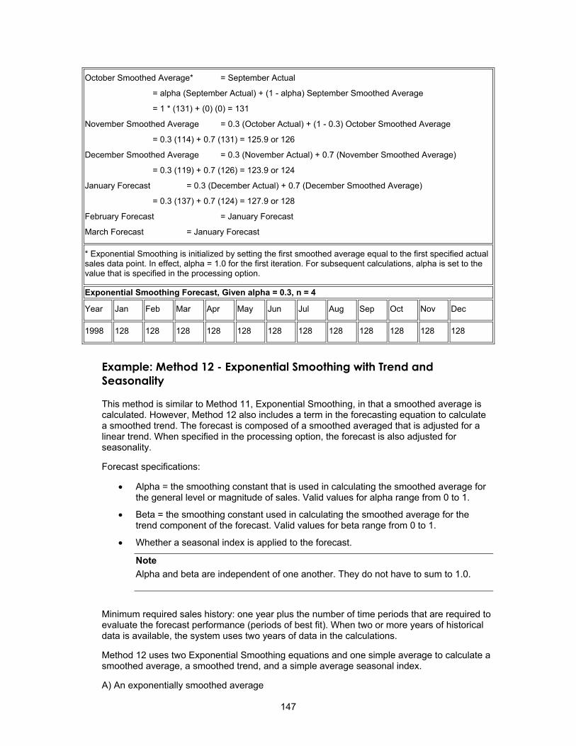
October Smoothed Average* = September Actual
= alpha (September Actual) + (1 - alpha) September Smoothed Average
= 1 * (131) + (0) (0) = 131
November Smoothed Average = 0.3 (October Actual) + (1 - 0.3) October Smoothed Average
= 0.3 (114) + 0.7 (131) = 125.9 or 126
December Smoothed Average = 0.3 (November Actual) + 0.7 (November Smoothed Average)
= 0.3 (119) + 0.7 (126) = 123.9 or 124
January Forecast = 0.3 (December Actual) + 0.7 (December Smoothed Average)
= 0.3 (137) + 0.7 (124) = 127.9 or 128
February Forecast = January Forecast
March Forecast = January Forecast
* Exponential Smoothing is initialized by setting the first smoothed average equal to the first specified actual sales data point. In effect, alpha = 1.0 for the first iteration. For subsequent calculations, alpha is set to the value that is specified in the processing option.
Exponential Smoothing Forecast, Given alpha = 0.3, n = 4
Year Jan Feb Mar Apr May Jun Jul Aug Sep Oct Nov Dec
1998 128 128 128 128 128 128 128 128 128 128 128 128
Example: Method 12 - Exponential Smoothing with Trend and Seasonality
This method is similar to Method 11, Exponential Smoothing, in that a smoothed average is calculated. However, Method 12 also includes a term in the forecasting equation to calculate a smoothed trend. The forecast is composed of a smoothed averaged that is adjusted for a linear trend. When specified in the processing option, the forecast is also adjusted for seasonality.
Forecast specifications:
• Alpha = the smoothing constant that is used in calculating the smoothed average for the general level or magnitude of sales. Valid values for alpha range from 0 to 1.
• Beta = the smoothing constant used in calculating the smoothed average for the trend component of the forecast. Valid values for beta range from 0 to 1.
• Whether a seasonal index is applied to the forecast.
Note Alpha and beta are independent of one another. They do not have to sum to 1.0.
Minimum required sales history: one year plus the number of time periods that are required to evaluate the forecast performance (periods of best fit). When two or more years of historical data is available, the system uses two years of data in the calculations.
Method 12 uses two Exponential Smoothing equations and one simple average to calculate a smoothed average, a smoothed trend, and a simple average seasonal index.
A) An exponentially smoothed average
147
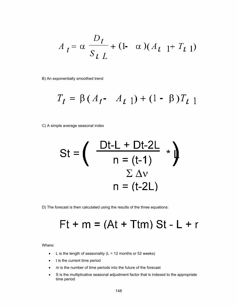
B) An exponentially smoothed trend
C) A simple average seasonal index
D) The forecast is then calculated using the results of the three equations:
Where:
• L is the length of seasonality (L = 12 months or 52 weeks)
• t is the current time period
• m is the number of time periods into the future of the forecast
• S is the multiplicative seasonal adjustment factor that is indexed to the appropriate time period
148
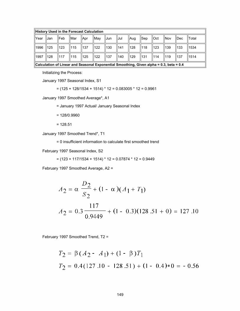
History Used in the Forecast Calculation
Year Jan Feb Mar Apr May Jun Jul Aug Sep Oct Nov Dec Total
1996 125 123 115 137 122 130 141 128 118 123 139 133 1534
1997 128 117 115 125 122 137 140 129 131 114 119 137 1514
Calculation of Linear and Seasonal Exponential Smoothing, Given alpha = 0.3, beta = 0.4
Initializing the Process:
January 1997 Seasonal Index, S1
= (125 + 128/1534 + 1514) * 12 = 0.083005 * 12 = 0.9961
January 1997 Smoothed Average*, A1
= January 1997 Actual/ January Seasonal Index
= 128/0.9960
= 128.51
January 1997 Smoothed Trend*, T1
= 0 insufficient information to calculate first smoothed trend
February 1997 Seasonal Index, S2
= (123 + 117/1534 + 1514) * 12 = 0.07874 * 12 = 0.9449
February 1997 Smoothed Average, A2 =
February 1997 Smoothed Trend, T2 =
149
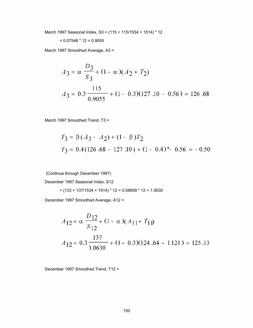
March 1997 Seasonal Index, S3 = (115 + 115/1534 + 1514) * 12
= 0.07546 * 12 = 0.9055
March 1997 Smoothed Average, A3 =
March 1997 Smoothed Trend, T3 =
(Continue through December 1997)
December 1997 Seasonal Index, S12
= (133 + 137/1534 + 1514) * 12 = 0.08858 * 12 = 1.0630
December 1997 Smoothed Average, A12 =
December 1997 Smoothed Trend, T12 =
150
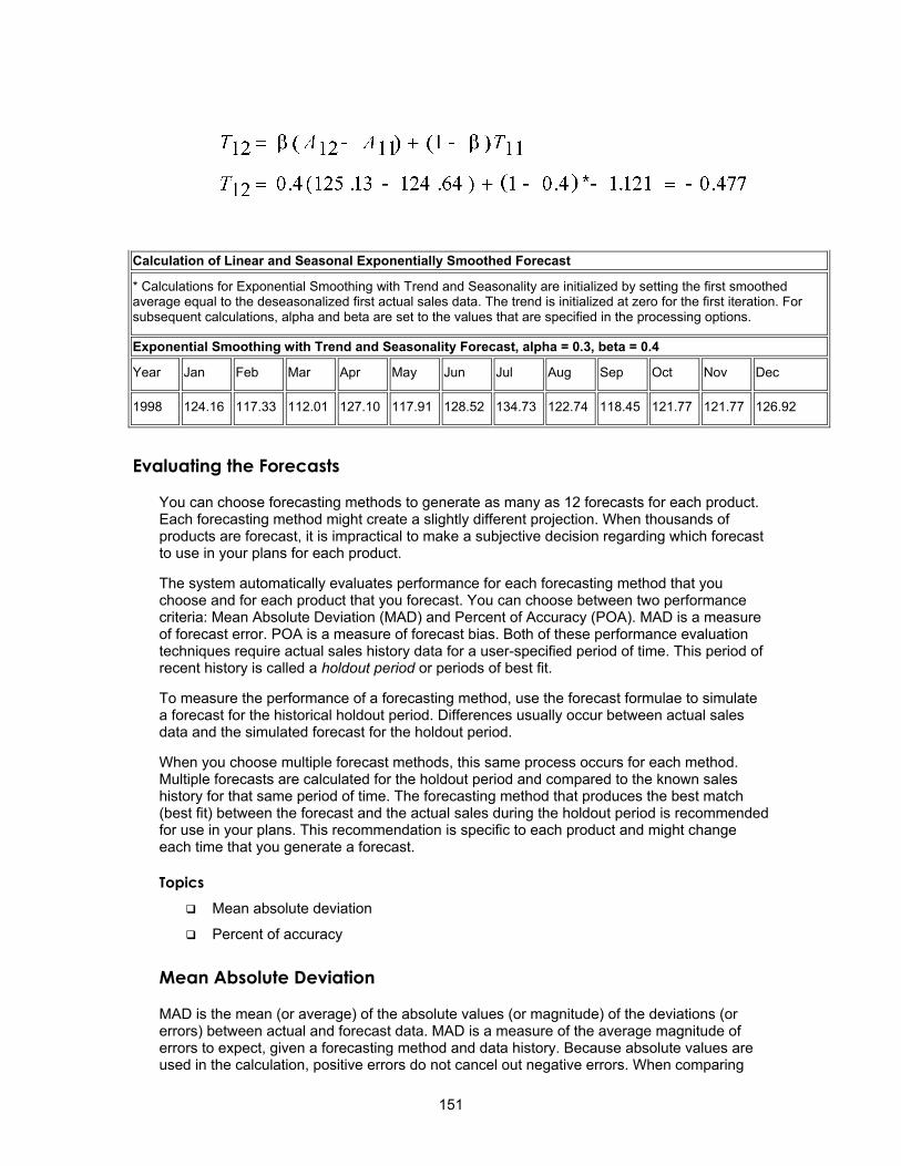
Calculation of Linear and Seasonal Exponentially Smoothed Forecast
* Calculations for Exponential Smoothing with Trend and Seasonality are initialized by setting the first smoothed average equal to the deseasonalized first actual sales data. The trend is initialized at zero for the first iteration. For subsequent calculations, alpha and beta are set to the values that are specified in the processing options.
Exponential Smoothing with Trend and Seasonality Forecast, alpha = 0.3, beta = 0.4
Year Jan Feb Mar Apr May Jun Jul Aug Sep Oct Nov Dec
1998 124.16 117.33 112.01 127.10 117.91 128.52 134.73 122.74 118.45 121.77 121.77 126.92
Evaluating the Forecasts
You can choose forecasting methods to generate as many as 12 forecasts for each product. Each forecasting method might create a slightly different projection. When thousands of products are forecast, it is impractical to make a subjective decision regarding which forecast to use in your plans for each product.
The system automatically evaluates performance for each forecasting method that you choose and for each product that you forecast. You can choose between two performance criteria: Mean Absolute Deviation (MAD) and Percent of Accuracy (POA). MAD is a measure of forecast error. POA is a measure of forecast bias. Both of these performance evaluation techniques require actual sales history data for a user-specified period of time. This period of recent history is called a holdout period or periods of best fit.
To measure the performance of a forecasting method, use the forecast formulae to simulate a forecast for the historical holdout period. Differences usually occur between actual sales data and the simulated forecast for the holdout period.
When you choose multiple forecast methods, this same process occurs for each method. Multiple forecasts are calculated for the holdout period and compared to the known sales history for that same period of time. The forecasting method that produces the best match (best fit) between the forecast and the actual sales during the holdout period is recommended for use in your plans. This recommendation is specific to each product and might change each time that you generate a forecast.
Topics Mean absolute deviation
Percent of accuracy
Mean Absolute Deviation
MAD is the mean (or average) of the absolute values (or magnitude) of the deviations (or errors) between actual and forecast data. MAD is a measure of the average magnitude of errors to expect, given a forecasting method and data history. Because absolute values are used in the calculation, positive errors do not cancel out negative errors. When comparing
151
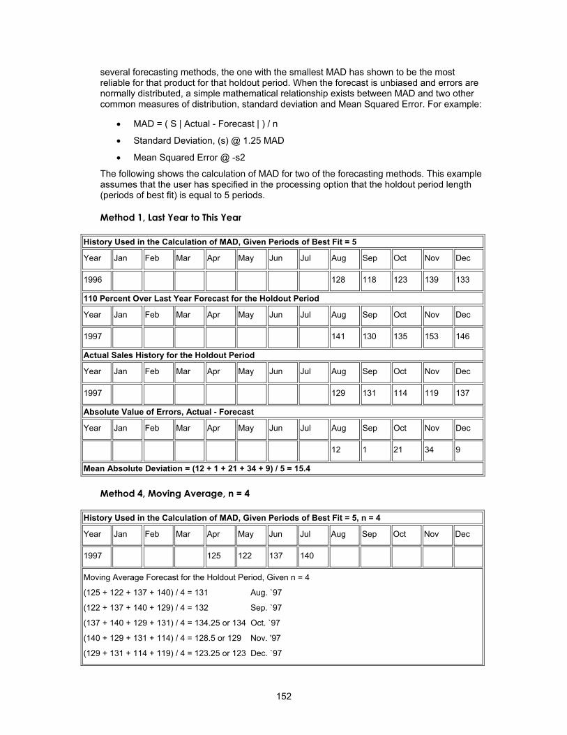
several forecasting methods, the one with the smallest MAD has shown to be the most reliable for that product for that holdout period. When the forecast is unbiased and errors are normally distributed, a simple mathematical relationship exists between MAD and two other common measures of distribution, standard deviation and Mean Squared Error. For example:
• MAD = ( S | Actual - Forecast | ) / n
• Standard Deviation, (s) @ 1.25 MAD
• Mean Squared Error @ -s2
The following shows the calculation of MAD for two of the forecasting methods. This example assumes that the user has specified in the processing option that the holdout period length (periods of best fit) is equal to 5 periods.
Method 1, Last Year to This Year
History Used in the Calculation of MAD, Given Periods of Best Fit = 5
Year Jan Feb Mar Apr May Jun Jul Aug Sep Oct Nov Dec
1996 128 118 123 139 133
110 Percent Over Last Year Forecast for the Holdout Period
Year Jan Feb Mar Apr May Jun Jul Aug Sep Oct Nov Dec
1997 141 130 135 153 146
Actual Sales History for the Holdout Period
Year Jan Feb Mar Apr May Jun Jul Aug Sep Oct Nov Dec
1997 129 131 114 119 137
Absolute Value of Errors, Actual - Forecast
Year Jan Feb Mar Apr May Jun Jul Aug Sep Oct Nov Dec
12 1 21 34 9
Mean Absolute Deviation = (12 + 1 + 21 + 34 + 9) / 5 = 15.4
Method 4, Moving Average, n = 4
History Used in the Calculation of MAD, Given Periods of Best Fit = 5, n = 4
Year Jan Feb Mar Apr May Jun Jul Aug Sep Oct Nov Dec
1997 125 122 137 140
Moving Average Forecast for the Holdout Period, Given n = 4
(125 + 122 + 137 + 140) / 4 = 131 Aug. `97
(122 + 137 + 140 + 129) / 4 = 132 Sep. `97
(137 + 140 + 129 + 131) / 4 = 134.25 or 134 Oct. `97
(140 + 129 + 131 + 114) / 4 = 128.5 or 129 Nov. '97
(129 + 131 + 114 + 119) / 4 = 123.25 or 123 Dec. `97
152
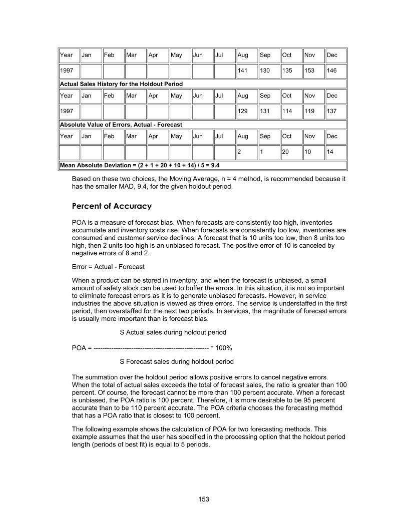
Year Jan Feb Mar Apr May Jun Jul Aug Sep Oct Nov Dec
1997 141 130 135 153 146
Actual Sales History for the Holdout Period
Year Jan Feb Mar Apr May Jun Jul Aug Sep Oct Nov Dec
1997 129 131 114 119 137
Absolute Value of Errors, Actual - Forecast
Year Jan Feb Mar Apr May Jun Jul Aug Sep Oct Nov Dec
2 1 20 10 14
Mean Absolute Deviation = (2 + 1 + 20 + 10 + 14) / 5 = 9.4
Based on these two choices, the Moving Average, n = 4 method, is recommended because it has the smaller MAD, 9.4, for the given holdout period.
Percent of Accuracy
POA is a measure of forecast bias. When forecasts are consistently too high, inventories accumulate and inventory costs rise. When forecasts are consistently too low, inventories are consumed and customer service declines. A forecast that is 10 units too low, then 8 units too high, then 2 units too high is an unbiased forecast. The positive error of 10 is canceled by negative errors of 8 and 2.
Error = Actual - Forecast
When a product can be stored in inventory, and when the forecast is unbiased, a small amount of safety stock can be used to buffer the errors. In this situation, it is not so important to eliminate forecast errors as it is to generate unbiased forecasts. However, in service industries the above situation is viewed as three errors. The service is understaffed in the first period, then overstaffed for the next two periods. In services, the magnitude of forecast errors is usually more important than is forecast bias.
S Actual sales during holdout period
POA = ---------------------------------------------------- * 100%
S Forecast sales during holdout period
The summation over the holdout period allows positive errors to cancel negative errors. When the total of actual sales exceeds the total of forecast sales, the ratio is greater than 100 percent. Of course, the forecast cannot be more than 100 percent accurate. When a forecast is unbiased, the POA ratio is 100 percent. Therefore, it is more desirable to be 95 percent accurate than to be 110 percent accurate. The POA criteria chooses the forecasting method that has a POA ratio that is closest to 100 percent.
The following example shows the calculation of POA for two forecasting methods. This example assumes that the user has specified in the processing option that the holdout period length (periods of best fit) is equal to 5 periods.
153
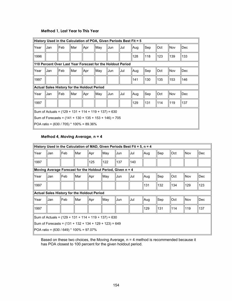
154
Method 1, Last Year to This Year
History Used in the Calculation of POA, Given Periods Best Fit = 5
Year Jan Feb Mar Apr May Jun Jul Aug Sep Oct Nov Dec
1996 128 118 123 139 133
110 Percent Over Last Year Forecast for the Holdout Period
Year Jan Feb Mar Apr May Jun Jul Aug Sep Oct Nov Dec
1997 141 130 135 153 146
Actual Sales History for the Holdout Period
Year Jan Feb Mar Apr May Jun Jul Aug Sep Oct Nov Dec
1997 129 131 114 119 137
Sum of Actuals = (129 + 131 + 114 + 119 + 137) = 630
Sum of Forecasts = (141 + 130 + 135 + 153 + 146) = 705
POA ratio = (630 / 705) * 100% = 89.36%
Method 4, Moving Average, n = 4
History Used in the Calculation of MAD, Given Periods Best Fit = 5, n = 4
Year Jan Feb Mar Apr May Jun Jul Aug Sep Oct Nov Dec
1997 125 122 137 140
Moving Average Forecast for the Holdout Period, Given n = 4
Year Jan Feb Mar Apr May Jun Jul Aug Sep Oct Nov Dec
1997 131 132 134 129 123
Actual Sales History for the Holdout Period
Year Jan Feb Mar Apr May Jun Jul Aug Sep Oct Nov Dec
1997 129 131 114 119 137
Sum of Actuals = (129 + 131 + 114 + 119 + 137) = 630
Sum of Forecasts = (131 + 132 + 134 + 129 + 123) = 649
POA ratio = (630 / 649) * 100% = 97.07%
Based on these two choices, the Moving Average, n = 4 method is recommended because it has POA closest to 100 percent for the given holdout period.