entrainment in an air/water system inside a sieve …

ENTRAINMENT IN AN AIR/WATER SYSTEM

INSIDE A SIEVE TRAY COLUMN

by

Ehbenezer Chris Uys

Thesis presented for the Degree

of

MASTER OF SCIENCE IN ENGINEERING

(CHEMICAL ENGINEERING)

in the Department of Process Engineering

at the University of Stellenbosch

Supervised by

Prof. J.H. Knoetze and Prof. A.J. Burger

STELLENBOSCH

MARCH 2010

Declaration

I, the undersigned, hereby declare that the work contained in this thesis is my own original

work and that I have not previously in its entirety or in part submitted it at any university for

a degree.

…………………………………….. ………………………………………

Signature Date

Copyright © 2010 Stellenbosch University

All rights reserved

ii

Abstract

Mass transfer efficiency in distillation, absorption and stripping depends on both

thermodynamic efficiency and hydrodynamic behaviour. Thermodynamic efficiency is

dependent on the system kinetics while hydrodynamics is the study of fluid flow behaviour.

The focus of this thesis is the hydrodynamic behaviour in tray columns, which affects

entrainment. In order to isolate hydrodynamic behaviour from the thermodynamic

behaviour that occurs inside sieve tray columns, investigations are conducted under

conditions of zero mass transfer. When the gas velocity is sufficiently high to transport liquid

droplets to the tray above, entrainment occurs. The onset of entrainment is one of the

operating limits that determines the design of the column and thus impacts on the capital

cost. By improving the understanding of the parameters that affect entrainment, the design

of the tray and column can be improved which will ultimately increase the operability and

capacity while reducing capital costs.

Existing correlations predicting entrainment in sieve tray columns are based on data

generated mainly from an air/water system. Previous publications recommend that more

testing should be performed over larger ranges of gas and liquid physical properties. An

experimental setup was therefore designed and constructed to test the influence of the

following parameters on entrainment:

1. gas and liquid physical properties

2. gas and liquid flow rates

3. tray spacing

The experimental setup can also measure weeping rates for a continuation of this project.

The hydrodynamic performance of a sieve tray was tested with air and water over a wide

range of gas and liquid flow rates and at different downcomer escape areas. It was found

that the downcomer escape area should be sized so that the liquid escaping the downcomer

always exceeds a velocity of approximately 0.23 m/s in order to create a sufficient liquid

seal in the downcomer. For liquid velocities between 0.23 and 0.6 m/s the area of escape

did not have an effect on the percentage of liquid entrained. It was also established that

entrainment increases with increasing gas velocity. The rate at which entrainment increases

as the gas velocity increase depends on the liquid flow rate. As soon as the liquid flow rate

exceeded 74 m3/(h.m) a significant increase in entrainment was noted and the gas velocity

had to be reduced to maintain a constant entrainment rate. This is because the increased

liquid load requires a longer flow path length for the froth to fully develop. The

undeveloped froth, caused by the short (455 mm) flow path, then creates a non-uniform

froth that is pushed up against the column wall above the downcomer. Consequently, the

iii

froth layer is closer to the tray above resulting in most of the droplets ejected from the froth

reaching the tray above and increasing entrainment. By reducing the gas velocity, the froth

height and ejecting droplet velocity is reduced, resulting in a decrease in entrainment.

The results from the experiments followed similar trends to most of the entrainment

prediction correlations found in literature, except for the change noted in liquid flow rates

above 74 m3/(h.m). There was, however, a significant difference between the experimental

results and the correlations developed by Hunt et al. (1955) and Kister and Haas (1988).

Although the gas velocities used during the air/water experiments were beyond the

suggested range of application developed by Bennett et al. (1995) their air/water

correlation followed the results very well.

The entrainment prediction correlation developed by Bennett et al. (1995) for non-air/water

systems was compared with the experimental air/water results to test for system

uniformity. A significant difference was noted between their non-air/water prediction

correlation and the air/water results, which motivates the need for a general entrainment

prediction correlation over a wider range of gas and liquid physical properties.

Based on the shortcomings found in the literature and the observations made during the

experiments it is suggested that the influence of liquid flow path length should be

investigated so that the effect on entrainment can be quantified. No single correlation was

found in the literature, which accurately predicts entrainment for a large range of liquid

loads (17 – 112 m3/(h.m)), high superficial gas velocities (3 – 4.6 m/s) and different gas and

liquid physical properties. It is therefore recommended that more work be done, as an

extension of this project, to investigate the influence of gas and liquid physical properties on

entrainment (under zero mass transfer conditions) for a large range of liquid (5 – 74

m3/(h.m)) and gas (2 – 4.6 m/s) flow rates. In order to understand the effect of droplet drag

on entrainment, tray spacing should be varied and increased to the extent where droplet

ejection velocity is no longer the mechanism for entrainment and droplet drag is responsible

for droplet transport to the tray above.

Since it is difficult and in most cases impossible to measure exact gas and liquid loads in

commercial columns, another method is required to measure or determine entrainment.

Since liquid hold-up was found to be directly related to the entrainment rate (Hunt et al.

(1955), Payne and Prince (1977) and Van Sinderen et al. (2003) to name but a few), it is

suggested that a correlation should be developed between the dynamic pressure drop

(liquid hold-up) and entrainment. This will contribute significantly to commercial column

operation from a hydrodynamic point of view.

iv

Acknowledgements

I would like to convey my sincere gratitude towards my supervisors Prof. J.H. Knoetze, Prof.

A.J. Burger and Dr. C.E. Schwarz for their continuous encouragement, patience, support and

critique.

Without the financial support from Sasol Pty (Ltd), the South African Department of Trade

and Industry through THRIP and Koch-Glitsch this project would not have been made

possible.

To my father, Dirk Uys, I want to extend my heartfelt and most sincere gratitude for

teaching me how to endure even at times when the answers don’t seem to come. You

taught me that giving up is not part of the equation to success. It is because you exposed me

to the mechanical side of engineering that I could develop the experimental setup required

for this work.

To my mother, Martie Uys, I will never forget your love and continuous motivation. Through

you I realised that even if you reached the pinnacle of success, without love life would have

no meaning.

To my close friend, Sarel Lamprecht, without your daily support, memorable moments and

reasoning through problems at times when the going was tough, I want to extent many

thanks. You are indeed a friend for life.

The Process Engineering workshop, Jannie Barnard, Anton Cordier and Howard Koopman,

should take the glory for helping with the construction of a versatile and brilliant

experimental setup.

v

Table of contents

Declaration ................................................................................................................................ i

Abstract .....................................................................................................................................ii

Acknowledgements .................................................................................................................. iv

Glossary .................................................................................................................................... ix

Abbreviations ............................................................................................................................ x

Nomenclature .......................................................................................................................... xi

List of figures .......................................................................................................................... xvi

List of tables ........................................................................................................................... xix

1 Introduction ................................................................................................................. 1

1.1 Background .................................................................................................................. 1

1.2 Introduction to hydrodynamics in tray columns ......................................................... 2

1.3 Project scope ................................................................................................................ 8

1.4 Objectives ..................................................................................................................... 9

1.5 Thesis layout............................................................................................................... 11

2 A historical overview of the hydrodynamic characterization in sieve tray

distillation columns .................................................................................................... 12

2.1 Work done on Hydrodynamic behaviour in Sieve Tray Columns .............................. 12

2.1.1 Hunt et al. (1955) – Capacity factors in the performance of perforated plate

columns. ..................................................................................................................... 12

2.1.2 Porter and Wong (1969) – The transition from spray to bubbling on sieve plates. .. 16

2.1.3 Lockett et al. (1976) – The effect of the operating regime on entrainment from

sieve trays................................................................................................................... 20

2.1.4 Payne and Prince (1977) – Froth and spray regimes on distillation plates. .............. 21

2.1.5 Thomas and Ogboja (1978) – Hydraulic studies in sieve tray columns. .................... 22

2.1.6 Hofhuis and Zuiderweg (1979) – Sieve plates: Dispersion density and flow

regimes. ...................................................................................................................... 26

2.1.7 Sakata and Yanagi (1979, 1982) – Performance of a commercial scale sieve tray. .. 29

2.1.8 Porter and Jenkins (1979) – The Interrelationship between industrial practice

and academic research in distillation and absorption. .............................................. 31

2.1.9 Kister et al. (1981) – Entrainment from sieve trays operating in the spray

regime. ....................................................................................................................... 33

vi

2.1.10 Colwell (1981) – Clear liquid height and froth density on sieve trays. ...................... 36

2.1.11 Zuiderweg (1982) – Sieve Trays: A view on the state of the art ................................ 39

2.1.12 Kister and Haas (1988) – Entrainment from sieve trays in the froth regime. ........... 42

2.1.13 Kister and Haas (1990) – Predict entrainment flooding on sieve and valve trays ..... 45

2.1.14 Bennett et al. (1995) – A mechanistic analysis of sieve tray froth height and

entrainment ............................................................................................................... 48

2.1.15 Jaćimović and Genić (2000) – Froth porosity and clear liquid height in trayed

columns ...................................................................................................................... 55

2.1.16 Van Sinderen et al. (2003) – Entrainment and maximum vapour flow rate of

trays. ........................................................................................................................... 56

2.2 Critical evaluation ...................................................................................................... 59

2.3 Summary of literature survey .................................................................................... 71

2.4 Scope for potential research ...................................................................................... 73

2.4.1 Scope for this work .................................................................................................... 73

3 Design of a distillation sieve tray column for hydrodynamic characterisation ......... 74

3.1 Introduction ............................................................................................................... 74

3.1.1 Objective .................................................................................................................... 74

3.1.2 Scope and Limitations ................................................................................................ 75

3.2 Concept design ........................................................................................................... 77

3.2.1 Pilot Plant Unit Selection ........................................................................................... 77

3.2.2 Pilot plant layout ........................................................................................................ 77

3.3 Detail design ............................................................................................................... 79

3.3.1 Choosing gas and liquid systems ................................................................................ 79

3.3.2 Column design ............................................................................................................ 82

3.3.3 Gas blower (E-102) ..................................................................................................... 88

3.3.4 Liquid pump (E-204) ................................................................................................... 88

3.3.5 Entrainment and weeping measuring vessels (MV-202, 203, 204) ........................... 89

3.3.6 Surge tank (E-101) design .......................................................................................... 91

3.3.7 Heat exchanger (E-205) design .................................................................................. 92

3.3.8 Venturi design (E-103) ................................................................................................ 93

3.3.9 System pressure control ............................................................................................ 93

3.3.10 Sensor placing ............................................................................................................ 93

vii

3.3.11 Sensor sizing and selection ........................................................................................ 95

3.3.12 HAZOP, Safety interlocks and control philosophy ..................................................... 96

3.3.13 Control system design ................................................................................................ 96

3.3.14 Data recording ............................................................................................................ 98

3.3.15 Piping and instrumentation diagram ......................................................................... 98

3.4 Experimental procedure .......................................................................................... 101

3.5 Factors affecting measurement accuracy ................................................................ 103

3.6 Data processing ........................................................................................................ 104

4 Experimental results & discussion ........................................................................... 105

4.1 Gas and liquid flow rates .......................................................................................... 105

4.2 Experimental results ................................................................................................ 106

4.2.1 Sensitivity analysis of the downcomer escape area on entrainment ...................... 106

4.2.2 Entrainment data ..................................................................................................... 110

4.3 Comparing results with predictive trends ............................................................... 116

4.3.1 Deviation between experimental data and predictive trend by Bennett et al.

(1995) ....................................................................................................................... 121

4.3.2 Comparison between experimental data and predictive trend by Bennett et al.

(1995) for a non-air/water (NAW) system ............................................................... 121

5 Conclusions .............................................................................................................. 123

6 Recommendations for future work ......................................................................... 126

7 References ................................................................................................................ 128

8 Appendix A ............................................................................................................... 130

8.1 Equipment design specifications.............................................................................. 130

8.1.1 Surge Tank Design .................................................................................................... 131

8.1.2 Heat exchanger design specifications ...................................................................... 132

8.2 Sensor design specifications .................................................................................... 133

8.2.1 Venturi design .......................................................................................................... 133

8.2.2 Sensor specification tables ....................................................................................... 137

8.3 HAZOP, Safety interlocks and control philosophy ................................................... 139

8.3.1 Safety interlocks ....................................................................................................... 144

8.3.2 Control philosophy ................................................................................................... 145

8.4 Verification of the experimental setup .................................................................... 146

viii

8.4.1 Calibrating and commissioning of the control system ............................................ 146

8.4.2 Calibrating entrainment and weeping hold-up tanks .............................................. 148

8.4.3 Testing system for leakages ..................................................................................... 150

8.4.4 Verification of sensor measurements ...................................................................... 150

8.4.5 Testing the system with Air and Water ................................................................... 153

8.5 Experimental data for air water at 25°C .................................................................. 156

8.6 Data processing ........................................................................................................ 168

ix

Glossary

Bubbling area

Measured as column area minus two downcomer areas.

Clear liquid height

The liquid inventory (hold-up) on and above the tray expressed as the height the

liquid will occupy when it is not a frothy gas liquid mixture. This can also be seen as

the pressure drop across the froth above (space between the trays) the tray.

Downcomer Escape Area

Clearance area under the downcomer apron (see Figure 1.2).

Dry tray pressure drop

The pressure drop across the tray without the presence (or effect) of liquid.

Entrainment

Entrainment occurs when the gas velocity is sufficiently high to transport liquid as

droplets to the tray above.

Gas Superficial velocity

Gas velocity based on the column net area (total column area minus one downcomer

area for single pass trays)

Fractional hole area

Fractional hole area is defined as the ratio of the total hole area over the area

covered by the holes.

Froth height

Height of the froth above the tray deck (see Figure 1.2).

Froth Regime

In the froth regime vapour passes through the liquid continuous layer in the form of

jets or a series of bubbles. The froth regime is formed by moderate to high liquid

flow rates and low to moderate vapour flow rates.

x

Liquid flow path length

The section of the tray where the liquid exits the downcomer and crosses the tray,

measured from the downcomer exit to the exit weir (see Figure 1.2).

Liquid hold-up

See the definition for clear liquid height.

Perforated area

Area of the tray covered with holes/perforations (see Figure 1.2).

Residual pressure drop

The total tray pressure drop minus dry tray pressure drop minus the equivalent

liquid head. This was defined by Hunt et al. (1955) which used a constant head tank

(no liquid cross flow) to manipulate and measure the liquid height above the tray.

Spray Regime

In the spray regime vapour is continuously jetting through the holes creating liquid

droplets. This regime is characterized by high vapour flow rates and low liquid flow

rates resulting in low liquid depths (hold-up) on the tray.

Weeping

Weeping occurs when the gas velocity is sufficiently low so that the liquid in the tray

is “dumped” through the tray perforations to the tray below.

Abbreviations

AW – Air/water

PLC – Programmable logic controller used as the main controller on the pilot plant.

NAW – Non air/water

MEK – Methyl ethyl ketone

xi

Nomenclature

Symbol Description Units

Ab Bubbling Area (Ac-2Ad) m2

Ac Column area m2

Ad Downcomer area m2

Ap Perforated (Active) area, including blank areas m2

Aap Clearance area under downcomer apron (Downcomer

Escape Area)

m2

Ah Total hole area m2

Ah* Total hole area ft2

An Net area available for vapour-liquid disengagement (Ac-Ad) m2

Af Fractional hole area (Ah/ Ap) or tray free area -

B Weir length per unit bubbling area m-1

Cb Capacity factor based on Ab, ( )/b b g L gC u ρ ρ ρ= −

m/s

CD Venturi discharge coefficient

Cp Capacity factor based on Ap, ( )/p p g L gC u ρ ρ ρ= −

m/s

Cs Capacity factor based on An, ( )/s s g L gC u ρ ρ ρ= −

m/s

Cf Flooding factor, Souders and Brown flooding constant m/s

DH Hole diameter m

dH Hole diameter mm

xii

dH* Hole diameter in

E Entrainment (mass liquid/mass vapour) -

Ef Entrainment in the froth regime (kg liquid/kg vapour) -

Es Entrainment in the spray regime (kg liquid/kg vapour) -

Ew Entrainment measured while weeping occurs

simultaneously (kg liquid/kg vapour) -

FS F-factor, gsF u ρ= (kg/m)

1/2/s

F* F-factor, gbF u ρ= (lb/ft)1/2

s

FP F-factor, gpF u ρ= (kg/m)

1/2/s

FP* F-factor, gpF u ρ= (lb/ft)1/2

s

G Gas/Vapour mass flow kg/s

g Gravitational constant, 9.81 m/s2

gc Gravitational constant, 32.2 lbm/(lbf.s2)

Hb Bed height m

hb Bed height mm

Hd Dynamic pressure drop m, water

hd Dynamic pressure drop mm, water

hd* Dynamic pressure drop in, water

HDP* Dry tray pressure drop ft, vapour

HF Froth height m

xiii

HFe Effective froth height (Developed by Bennett et al. (1995)) m

hF Froth height mm

hf* Froth height in

Hf,t Froth/Dispersion height at the froth to spray transition m

HL Clear liquid height m

HL,tr Clear liquid height at the low – to – high-liquid layer

transition, see Van Sinderen et al. (2003)

m

hL Clear liquid height mm

hL,f Clear liquid height in froth regime mm

hL,t Clear liquid height at the froth to spray transition mm

hL,t* Clear liquid height at the froth to spray transition in

hM Momentum heads mm, water

HR Residual pressure drop m, water

Ht Total tray pressure drop m, water

ht* Total tray pressure drop in, water

Hw Weir height m

hw Weir height mm

L Liquid mass flow (Entering the tray from the downcomer) kg/s

L’ Entrained liquid mass flow kg/s

l Weir length m

qL Liquid flow per weir length m3/(s.m)

xiv

P Hole pitch m

p Hole pitch mm

QL Liquid flow per weir length m3/(h.m)

QL* Liquid flow per weir length (US)gpm/ft

QL+

Liquid flow per weir length (Imp)gpm/ft

Qv Gas volumetric flow rate m3/s

R Gas constant J/(kg.K)

S Tray spacing m

s Tray spacing mm

S* Tray spacing in

uc Gas velocity based on column area m/s

uD0 Droplet ecjection velocity m/s

ub Gas/vapour velocity based on Ab m/s

uh Gas/vapour hole velocity based on Ah m/s

uh* Gas/vapour hole velocity based on Ah* ft/s

uL Liquid escape velocity, based on Aap m/s

up Gas/vapour velocity based on Ap m/s

up* Gas/vapour velocity based on Ap ft/s

us Superficial vapour velocity based on An m/s

ut Droplet terminal velocity m/s

ut* Droplet terminal velocity ft/s

xv

Vg Gas volumetric flow rate m3/s

Vl Liquid volumetric flow rate m3/s

Greek Symbols

ε Froth density as clear liquid fraction -

ρg Gas/vapour density kg/m3

ρL Liquid density kg/m3

σ Liquid surface tension mN/m

µ Liquid viscosity mPa.s

ζ Correction term for Eq. 2.38 defined by Eq. 2.39

xvi

List of figures

Figure 1.1 Illustration of vapour and liquid flow paths in a tray column ................................... 3

Figure 1.2 Contacting inside a tray column. [Adapted with permission from: Separation

Process Principles; J.D. Seader and Ernest J. Henley; Copyright © 1998 John

Wiley & Sons, Inc.]. .................................................................................................. 3

Figure 1.3 The three tray opening types for liquid and vapour contacting: (a) sieve or

perforation; (b) floating valve; (c) bubble cap. [Reprinted with permission of

John Wiley & Sons Inc., Separation Process Principles; J.D. Seader and Ernest

J. Henley; Copyright © 1998 John Wiley & Sons, Inc.] ............................................ 4

Figure 1.4 The flow regime diagram redrawn from Hofhuis and Zuiderweg (1979) .................. 6

Figure 1.5 Schematic representation of the influence of entrainment on the separation

efficiency. ................................................................................................................. 7

Figure 2.1 The timeline followed in the literature review. ....................................................... 12

Figure 2.2 Effect of plate spacing on entrainment, redrawn from Hunt et al. (1955) Fig. 9. ... 15

Figure 2.3 Effect of liquid flow rate on entrainment, redrawn from Fig 2 in Lockett et al.

(1976). .................................................................................................................... 21

Figure 2.4 The influence of vapour and liquid flow rates on entrainment. ............................. 31

Figure 2.5 Minimum Entrainment trend based on data from Sakata and Yanagi (1979) ........ 32

Figure 2.6 Transition between spray to mixed and mixed to emulsified regimes, redrawn

from Porter and Jenkins (1979) Fig. 13. ................................................................. 33

Figure 2.7 Difference in froth height between the solution which accounts for droplet

drag and no drag assumption by Bennett et al., based on the Froude and

Weber numbers, and the Vs = uD/uD0 ratio redrawn from Fig. 1 in Bennett et

al. (1995) ................................................................................................................ 50

Figure 2.8 Section view of the experimental setup used by Sinderen et al. (2003) ................. 57

Figure 2.9. Comparing the effect of gas velocity on entrainment between the different

entrainment prediction correlations. Dotted lines indicate extrapolation

beyond recommended range of application. ........................................................ 65

Figure 2.10 Investigating the influence of liquid flow rate on entrainment for the

different entrainment prediction correlations, plotted as (a) mass entrained

liquid per mass rising vapour (b) mass entrained liquid per mass liquid

entering the tray under exactly the same conditions. Dotted lines indicate

extrapolation beyond recommended range of application or testing. ................. 67

Figure 2.11 Investigating the influence of tray spacing on entrainment for the different

entrainment prediction correlations. Dotted lines indicate extrapolation

beyond recommended range of application or testing. ........................................ 69

Figure 2.12 Investigating the influence of (a) gas and (b) liquid flow rate on entrainment

for the different entrainment prediction correlations. ......................................... 70

Figure 3.1 Schematic representation of the pilot plant setup.................................................. 78

xvii

Figure 3.2 Column front view with dimensions in millimetres. ................................................ 83

Figure 3.3 Column side-and-isometric views with dimensions in millimetres. ........................ 84

Figure 3.4 Picture of a sieve tray used in this work. ................................................................. 86

Figure 3.5 Top view of the mist eliminator pad. ....................................................................... 87

Figure 3.6. Entrainment measuring hold-up tank configuration for larger entrained

liquid rates (L’ > 0.07kg/s). ..................................................................................... 90

Figure 3.7 Entrainment measuring hold-up tank configuration for small entrained liquid

rates (L’ < 0.07kg/s). ............................................................................................... 90

Figure 3.8 The Piping and Instrumentation Diagram of the experimental setup .................... 99

Figure 3.9 The Piping and Instrumentation Diagram of the hot-and-cold water supply

section. ................................................................................................................. 100

Figure 3.10 Detailed drawing of some of the components of the experimental setup. ........ 100

Figure 4.1 The influence of the downcomer escape area on entrainment as a function of

the capacity factor ( )/p p g L gC u ρ ρ ρ= − for a liquid flow rate of 28.6 m

3/(h.m). .... 107


the capacity factor ( )/p p g L gC u ρ ρ ρ= − for a liquid flow rate of 40 m

3/(h.m). ........ 108


the capacity factor ( )/p p g L gC u ρ ρ ρ= − for a liquid flow rate of 57.2 m

3/(h.m). ..... 109

Figure 4.4 The influence of the capacity factor (gas velocity) on entrainment for

individual liquid flow rate settings from 17.2 – 74.2 m3/(h.m) ........................... 111

Figure 4.5 The influence of the capacity factor (gas velocity) on entrainment for

individual liquid flow rate settings from 79.9 –112.9 m3/(h.m) .......................... 112

Figure 4.6 Influence of gas and liquid rates on entrainment where entrainment is

measured as mass liquid entrained per mass of liquid entering the tray. .......... 113

Figure 4.7 Influence of gas and liquid rates on entrainment where entrainment is

measured as mass liquid entrained per mass of rising vapour. .......................... 114

Figure 4.8 (a) Uniform developed froth. (b) Non-uniform developed froth. ......................... 115

Figure 4.9 Comparing the different methods of measuring the entrainment rate. ............... 116

Figure 4.10 Comparing entrainment predictive trends with experimentally generated

entrainment data with entrainment measured as L’/L. ...................................... 117

Figure 4.11 Comparing entrainment predictive trends with experimentally generated

entrainment data where entrainment is measured as L’/G. ............................... 118

Figure 4.12 Comparison between the experimental data and that of Bennett et al.

(1995) for 5 and 20% entrainment. ..................................................................... 120

Figure 4.13 Comparison between the experimental data and that of Bennett et al.

(1995) for 5% non-air/water (NAW) and air/water (AW) entrainment

prediction. ............................................................................................................ 122

Figure 8.1 Vertical liquid-vapour Separator ............................................................................ 131

Figure 8.2 Physical dimensions of the Venturi ....................................................................... 135

Figure 8.3 Velocity profile across a pipe section .................................................................... 151

xviii

Figure 8.4 The area under the graph method was used to determine the average

volumetric flow rate across the gas pipeline for each volumetric flow rate. ...... 151

Figure 8.5 Entrainment data collected at four different dates for a liquid flow rate of

57.3 m3/(h.m) ....................................................................................................... 155

Figure 8.6 Fitting trendlines to entrainment data for each liquid flow rate

[17.2 – 74.2 m3/(h.m)] as a function of entrainment. ......................................... 169

Figure 8.7 Fitting trendlines to entrainment data for each liquid flow rate

[79.9 – 112.9 m3/(h.m)] as a function of entrainment. ....................................... 169

Figure 8.8 Verification of the fitted correlation for entrainment against the data ................ 170

xix

List of tables

Table 1.1 Comparing the different tray types (Seader and Henley 1998) .................................. 4

Table 1.2 The structural layout of the thesis. ........................................................................... 11

Table 2.1 Summary of the column geometry, test ranges and systems used by Hunt et al.

(1955) ..................................................................................................................... 15

Table 2.2 Summary of the column geometry, test ranges and systems used by Porter and

Wong (1969)........................................................................................................... 17

Table 2.3 Experimental conditions used by Porter and Wong (1969). ..................................... 17

Table 2.4 Summary of the column geometry, test ranges and systems used by Lockett et

al. (1976). ............................................................................................................... 20

Table 2.5 Summary of the column geometry, test ranges and systems used by Payne and

Prince (1977). ......................................................................................................... 22

Table 2.6 Summary of the column geometry, test ranges and systems used by Thomas

and Ogboja (1978) .................................................................................................. 23

Table 2.7 Summary of the column geometry, test ranges and systems used by Hofhuis

and Zuiderweg (1979) ............................................................................................ 27

Table 2.8 Summary of the column geometry, test ranges and systems used by Sakata

and Yanagi (1979) .................................................................................................. 30

Table 2.9 Range of data used for correlating by Kister et al. (1981) ........................................ 34

Table 2.10 Range of data used for correlating by Colwell (1981) ............................................ 37

Table 2.11 Recommended range of application for Eq. 2.38, 2.41 and 2.43. .......................... 45

Table 2.12 Recommended range of application for Eq. 2.46 ................................................... 47

Table 2.13 Data used by Bennett et al. (1995) ......................................................................... 48

Table 2.14 System parameter range used by Bennett et al. (1995) ......................................... 54

Table 2.15 Range of data used for correlating by Jaćimović and Genić (2000) ........................ 55

Table 2.16 Range of data used for correlating by Van Sinderen et al. (2003) .......................... 57

Table 2.17 Application range summary of entrainment predictive correlations from

literature. ............................................................................................................... 60

Table 2.18 Parameter ranges used to compare different entrainment prediction

correlations. ........................................................................................................... 65

Table 3.1 Vapour/liquid physical properties found in commercial stripping and

distillation applications .......................................................................................... 80

Table 3.2 Approximated Gas Properties ................................................................................... 81

Table 3.3 Approximated Liquid Properties ............................................................................... 81

Table 3.4 Sieve Tray and Column Geometry. ........................................................................... 85

Table 3.5 Summary of Energy balance for the pilot plant ........................................................ 92

Table 4.1 Gas and liquid flow rate ranges used during testing. ............................................. 105

Table 4.2 Liquid velocity for each liquid flow rate against the downcomer escape area ...... 109

Table 4.3 Air/Water system physical properties used during experimental runs. ................. 110

xx

Table 8.1 Blower Design Specifications .................................................................................. 130

Table 8.2 Design specifications for the liquid pump............................................................... 130

Table 8.3 Surge Tank Geometry .............................................................................................. 132

Table 8.4 Heat Exchanger Design Specifications .................................................................... 133

Table 8.5 Digital differential pressure transmitter specifications .......................................... 137

Table 8.6 Digital absolute pressure transmitters.................................................................... 137

Table 8.7 Liquid flow meter specifications summary ............................................................. 138

Table 8.8 Gas mass flow meter specifications summary ........................................................ 138

Table 8.9 Hazard and operability table ................................................................................... 139

Table 8.10 Control system interlocks...................................................................................... 144

Table 8.11 Pilot plant control philosophy ............................................................................... 145

Table 8.12 The CALOG – PRO specifications ........................................................................... 146

Table 8.13 The CALOG – TEMP specifications ........................................................................ 147

Table 8.14 Calibration results for the hold-up vessels (MV-202/3) ....................................... 149

Table 8.15 Calibration results for the hold-up vessel (MV-204) ............................................. 149

Table 8.16 Calibrated area results for the hold-up vessels (MV-202/3/4) ............................. 150

Table 8.17 Verification of venturi measurements .................................................................. 152

Table 8.18 Liquid flow meter measurement verification ....................................................... 152

Table 8.19 Calculated measurement accuracies. ................................................................... 154

Table 8.20 Calculating maximum deviation expected from venturi mass flow meter using

Eq. 8.3. .................................................................................................................. 154

Table 8.21 Experimental entrainment data for 17.2 m3/(h.m) setting and

Aesc = 3.33×10-3

m2. .............................................................................................. 156


Aesc = 3.33×10-3

m2, 5.4×10

-3 m

2 and 8.575×10

-3 m

2 ............................................ 157

Table 8.23 Experimental entrainment data for 40 m3/(h.m) setting and

Aesc = 3.33×10-3

m2, 5.4×10

-3 m

2 and 8.575×10

-3 m

2 ............................................ 159


Aesc = 5.4×10-3

m2 and 8.575×10

-3 m

2 ................................................................... 161


Aesc = 5.4×10-3

m2 and 8.575×10

-3 m

2 ................................................................... 164


Aesc = 8.575×10-3

m2 ............................................................................................. 164


Aesc = 8.575×10-3

m2 ............................................................................................. 165


Aesc = 8.575×10-3

m2 ............................................................................................. 167

1

1 Introduction

The most common method available to separate liquid mixtures with different volatilities is

distillation. Distillation is a physical separation method conducted by boiling a liquid mixture

and using energy as a separation agent. As the temperature of the mixture increases the

more volatile component will reach boiling point first and escape from the liquid mixture as

a vapour while the less volatile component remains a liquid. Distillation is used

commercially for numerous applications. Crude oil is separated into components which are

used for transport, power generation, heating and packaging to name but a few. Old

desalination plants used distillation to separate water from salt. To produce nitrogen,

oxygen and argon on industrial scale, air is distilled at very low temperature.

In order to purify a gas/vapour stream with constituents that can dissolve in an absorbent,

an absorption process is used. The gas is brought into contact with the liquid absorbent

where the constituents in the gas dissolve in the liquid to varying extents based on their

solubilities. Commercially, carbon dioxide is separated from combustion products by

absorption with aqueous solutions of ethanolamine.

Stripping is the inverse of absorption during which a liquid mixture is purified with a gas or

vapour stripping agent. The objective is to create a favourable environment for the

component in the liquid phase to transfer to the vapour phase and hence stripping is

conducted at elevated temperatures and atmospheric, or lower, pressure. Steam stripping is

generally used to remove volatile organic components (which are partially soluble in water)

from waste water.

1.1 Background

Distillation, absorption and stripping are of the largest and most widely used separation

processes in the separations industry. In distillation both thermodynamic and hydrodynamic

behaviour determine the degree of separation (the separation efficiency) that can be

achieved between two or more components. Thermodynamic behaviour focuses on the

mass transfer efficiency and kinetics while hydrodynamics is the study of the fluids in

motion. This thesis addresses the hydrodynamic behaviour occurring inside sieve tray

columns.

Distillation is commonly used when liquid mixtures with different relative volatilities that are

thermally stable, with little or no corrosive properties have to be separated on a large scale.

Inside distillation columns contacting devices are used to create a mass transfer interface

2

between the less dense and more dense phases. These devices are divided into three main

groups known as structured packing, random packing and trays. Each group of contacting

devices has a unique application based on system parameters, operating conditions and

column geometry. Random packing is generally used in smaller diameter columns when

working with corrosive liquids where plastic or ceramic materials are preferred over metals.

Packed columns are preferred over tray columns in applications where foaming may be

severe and when the pressure drop must be low. Tray columns can be designed, scaled up

with more reliability, and are less expensive than packed columns (Seader and Henley 1998).

Columns with random packing are generally used when liquid velocities are high while tray

columns are used for low to medium liquid velocities (Seader and Henley, 1998).

1.2 Introduction to hydrodynamics in tray columns

A tray column is a vertical, cylindrical vessel in which vapour and liquid are contacted on a

series of trays (plates). The vapour and liquid flow counter-currently inside the column, as

shown in Figure 1.1 and Figure 1.2. The liquid flows across each tray, exiting over an outlet

weir into a downcomer which transfers the liquid by gravity to the tray below. The amount

of liquid on and above the tray is defined as the liquid hold-up and expressed as the clear

liquid height. The clear liquid height is therefore the pressure drop across the liquid froth,

measured in vertical meters (hydrostatic pressure) of the specific liquid.

A great deal of work has been done on hydrodynamics in tray columns, including:

1. Tray pressure drop (Hunt et al. 1955, Thomas & Ogboja (1978)).

2. Froth density and height (Thomas & Ogboja (1978), Hofhuis and Zuiderweg (1979),

Bennett et al. (1995), Jaćimović and Genić (2000)).

3. Flow regime definitions (Zuiderweg (1982), Kister and Haas (1988), Bennett et al.

(1995)).

4. Entrainment (Hunt et al. 1955, Thomas & Ogboja (1978), Kister and Haas (1988),

Bennett et al. (1995)).

5. Downcomer flooding (Zuiderweg (1982)).

6. The influences of fractional hole area (free area) of the tray on the hydrodynamic

behaviour (Thomas & Ogboja (1978)).

7. The influence of weir height (Van Sinderen et al. (2003))

8. The influence of tray spacing (Hunt et al. 1955, Thomas & Ogboja (1978))

Figure 1.1 Illustration of

Figure 1.2 Contacting inside a tray column. [Adapted

J.D. Seader and Ernest J. Henley; Copyright © 1998 John Wiley & Sons, Inc.].

Tray Geometry:

Vapour rises upward through both the openings in the tray and the liquid on the tray.

Openings in the tray can range between perforation (commonly referred to as sieve), valves,

or bubble caps (see Figure 1.

sieve tray is also the least expensive of all the tray types. The vapour passes through

perforations, or holes (3.2 – 25.4mm diameter), made in

High concentration

more volatile

component in vapour

phase

Illustration of vapour and liquid flow paths in a tray column

Contacting inside a tray column. [Adapted with permission from: Separation Process Principles;


d through both the openings in the tray and the liquid on the tray.


.3). The simplest and most common type is the sieve tray.

the least expensive of all the tray types. The vapour passes through

25.4mm diameter), made in sheet metal.

High concentration

less volatile

component in liquid

phase

3

vapour and liquid flow paths in a tray column.

from: Separation Process Principles;


d through both the openings in the tray and the liquid on the tray.


). The simplest and most common type is the sieve tray. The

the least expensive of all the tray types. The vapour passes through

concentration

component in liquid

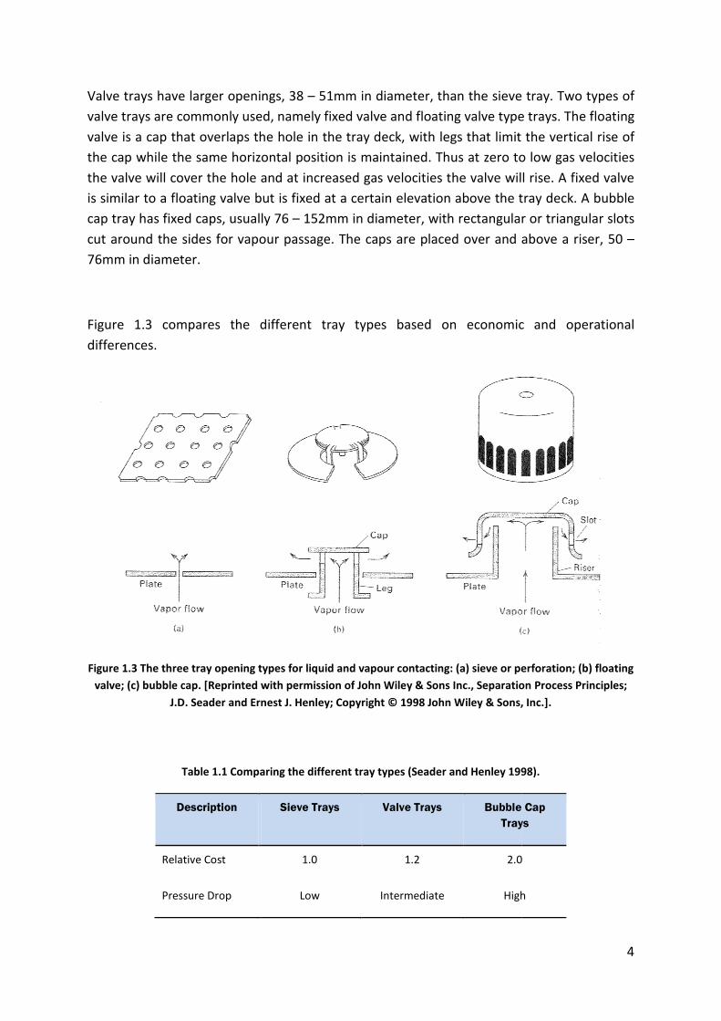
Valve trays have larger openings, 38

valve trays are commonly used, namely

valve is a cap that overlaps the hole in the tray deck

the cap while the same horizontal position is maintained. Thus at zero to low gas velocities

the valve will cover the hole and

is similar to a floating valve but is

cap tray has fixed caps, usually

cut around the sides for vapour passage. The caps are placed over and above a riser, 50

76mm in diameter.

Figure 1.3 compares the different tray types based on economic and operational

differences.

Figure 1.3 The three tray opening types for liquid and vapou

valve; (c) bubble cap. [Reprinted with permission of John Wiley & Sons Inc., Separation Process Principles;


Table 1.1 Comparing the different tray types (Seader and Henley 1998).

Description

Relative Cost

Pressure Drop

Valve trays have larger openings, 38 – 51mm in diameter, than the sieve tray. Two types of

trays are commonly used, namely fixed valve and floating valve type trays. The floating

valve is a cap that overlaps the hole in the tray deck, with legs that limit


the valve will cover the hole and at increased gas velocities the valve will rise

but is fixed at a certain elevation above the tray deck.

usually 76 – 152mm in diameter, with rectangular or triangular slots

cut around the sides for vapour passage. The caps are placed over and above a riser, 50

compares the different tray types based on economic and operational

The three tray opening types for liquid and vapour contacting: (a) sieve or perforation; (b) floating



Comparing the different tray types (Seader and Henley 1998).

Sieve Trays Valve Trays Bubble Cap

Trays

1.0 1.2 2.0

Low Intermediate High

4

51mm in diameter, than the sieve tray. Two types of

fixed valve and floating valve type trays. The floating

the vertical rise of


at increased gas velocities the valve will rise. A fixed valve

fixed at a certain elevation above the tray deck. A bubble

152mm in diameter, with rectangular or triangular slots

cut around the sides for vapour passage. The caps are placed over and above a riser, 50 –

compares the different tray types based on economic and operational

r contacting: (a) sieve or perforation; (b) floating



Comparing the different tray types (Seader and Henley 1998).

Bubble Cap

Trays

2.0

High

5

Table 1.1 Comparing the different tray types (Seader and Henley 1998).

Description Sieve Trays Valve Trays Bubble Cap

Trays

Efficiency Low High High

Vapour Capacity High High High

Turndown Ratio 2 4 5

The turndown ratio is the ratio of the gas flow rate at the onset of entrainment to the

minimum gas rate when the liquid weeps through the perforations. Since the sieve tray is

the simplest tray design, this thesis will focus on entrainment in sieve tray columns.

Tray hydraulics:

In the case where the tray openings are holes, different two-phase-flow regimes can be

encountered. Hofhuis and Zuiderweg (1979) defined four (see Figure 1.4) flow regimes

namely the spray regime, the mixed froth regime, the free bubbling regime, and the

emulsified flow regime. They suggest that the spray regime is significant for applications

operating under vacuum while the emulsion flow regime applies to high pressure distillation

and high liquid load absorption. From the flow regime diagram (Figure 1.4) it can be seen

that gas and liquid density will influence the operating flow regime. They suggest that

viscosity and surface tension have little or no effect on the flow regime.

Most of the work done in literature focuses on the spray regime, mixed regime (transition

from emulsified to spray regime) and the froth regime (which represents the emulsified

regime). Each author defines and determines the regimes differently. According to Seader

and Henley (1998) the most favoured regime is the froth regime in which the vapour passes

through the liquid continuous layer in the form of jets or a series of bubbles. The mixed

froth regime is formed by moderate to high liquid flow rates and low to moderate vapour

flow rates. In the spray regime the vapour is continuously jetting through the holes, creating

liquid droplets. This regime is characterized by high vapour flow rates and low liquid flow

rates resulting in low liquid depths (hold-up) on the tray.

6

Figure 1.4 The flow regime diagram redrawn from Hofhuis and Zuiderweg (1979).

At low vapour flow rates and moderate liquid flow rates the bubble regime occurs where

bubbles rise through the quiescent liquid layer. At high liquid and low to moderate vapour

rates the emulsion (froth) flow regime can occur. In the emulsion regime small gas bubbles

can be undesirably suspended in the liquid.

In order to express and correlate hydrodynamic behaviour dimensionless numbers or

modified (from the known/common groupings) dimensionless numbers are used. The most

common dimensionless numbers used to characterise hydrodynamic behaviour in tray

columns are:

1. The Froude number (2

0D

F

uFr

gH= ) or ( b

L

uFr

gH= ) where uD0 is the droplet ejection

velocity, g is gravitational acceleration, HF is the froth height, ub is the gas velocity

based on the tray bubbling area and HL is the clear liquid height.

2. The Bond number (

2gLBo

ρσ

= ) where ρ is the density or the density difference of

the fluid/s, g is gravitational acceleration, L is a characteristic length (normally

droplet diameter or hole diameter) and σ is the liquid surface tension.

Mixed Froth

Spray

Emulsion

Flooding Limit

Weeping Limits

ρl = 500 kg/m3

ρl = 1000 kg/m3

gb b

l g

C uρ

ρ ρ=

−

l l

b g

u

u

ρφρ

=

Free Bubbling

0.01 1.00.1

1.0

0.02

0.04

0.06

0.08

7

3. The Weber number (

2v lWe

ρσ

= ) where ρ is the density of the fluid, ν its velocity, l is

a characteristic length and σ is the liquid surface tension.

The Froude number compares the inertia forces with the gravitational force acting on an

object and is based on a speed over length ratio. The Bond number is the ratio of

gravitational (or body forces) to surface tension forces. To compare the inertia of a fluid

with its surface tension the Weber number is used. The Weber number is useful in analysing

the flow behaviour of thin films and the formation of droplets and bubbles.

Entrainment:

When the velocity of the gas is sufficiently high to transport liquid droplets to the tray

above, liquid entrainment occurs. This influences the mass transfer separation efficiency, as

shown in Figure 1.5, since the entrained liquid contains a higher fraction of the less volatile

component than the liquid on the tray above. This increases the concentration of the less

volatile component on the tray above. The onset of entrainment is one of the operating

parameters which constrain the mass transfer separation efficiency. The maximum

allowable entrainment is achieved when the separation efficiency on each tray is reduced to

the point where the overall required separation cannot be obtained with the number of

trays available in the column. Therefore the onset of entrainment is a vital parameter in the

design of the column and thus directly impacts the cost.

Figure 1.5 Schematic representation of the influence of entrainment on the separation efficiency.

The study of entrainment is categorised as part of the hydrodynamic behaviour inside the

distillation column and is generally influenced by the following parameters:

1. Gas and liquid flow rates

High concentration less volatile

component in liquid phase

Entrained liquid droplets in

vapour space above the froth

layer.

Entrained liquid droplets present

in liquid on tray above,

increasing fraction of low

volatile component and reducing

separation efficiency.

8

2. Gas and liquid physical properties

3. Column and tray geometry

Weeping:

Another hydrodynamic phenomenon is found when the vapour rate is low enough for liquid

dumping (weeping) to occur. Under these conditions the vapour rate is so low that the

liquid weeps through the holes in the tray to the tray below. Weeping is therefore the

inverse of entrainment and also negatively influences the separation efficiency.

Flooding:

Excessive entrainment can cause the liquid flow rate to exceed the downcomer capacity

(Seader and Henley, 1998). As the downcomer exceeds capacity, liquid will build-up on the

trays and go back up the column causing the column to flood. Column flooding can also

occur when the liquid feed flow rate exceeds the downcomer capacity while the gas flow

rate is sufficiently high enough to prevent weeping, resulting in a liquid build-up on the tray.

Another mechanism for column flooding occurs during low liquid rates when the vapour

velocity is high enough so that the amount of liquid entrained exceeds the liquid rate

flowing through the downcomer (and column).

1.3 Project scope

In this study the focus is on entrainment and the hydrodynamic behaviour that constitutes

entrainment. In order to investigate the hydrodynamic behaviour inside the tray column it

was decided to use a thermally stable gas and liquid system (air/water) to ensure that no

mass transfer occurred between the phases. To further simplify the investigation it was

decided not to test the effects of foaming on entrainment.

Currently the entrainment rate is expressed and measured as the mass of liquid entrained

over the mass of rising vapour (Hunt et al. (1955), Kister and Haas (1988) and Bennett et al.

(1995)). This expression does not consider the amount of liquid on the tray and can

therefore not be linked to the rate of liquid entrained compared to the liquid flow rate

entering the tray. A correlation is therefore required to predict entrainment as a function of

the liquid entering the tray so that the effect of entrainment on the separation efficiency

can be determined directly.

Work has been done on the effect that gas and liquid flow rates, tray geometry, tray spacing

and weir height have on entrainment. Since most of the work done in the literature focused

on entrainment in the spray regime for low liquid loads. Very little is mentioned about the

hydrodynamic behaviour at excessive entrainment for high liquid (> 45m3/(h.m)) and vapour

9

loads (> 3m/s). No extensive research has been done on the effects that gas and liquid

physical properties have on entrainment because most of the work has been done with the

air/water system, resulting in a lack of non-air/water system data. The limited existing non-

air/water data is obtained from various sources with different column geometries and

sampling methods.

Based on the shortcomings in the literature there is a need to generate entrainment data

over a wide range of experimental conditions including conditions of excessive entrainment.

The data should be generated by using a range of gas/liquid systems so that the influence of

system (gas and liquid) physical properties on entrainment can be determined. To eliminate

the effect of different column geometries and sampling methods, one experimental setup of

known geometry should be used to generate entrainment data. Foaming is another

hydrodynamic phenomenon that negatively affects mass transfer in distillation and

especially stripping applications. However, due to the limited time available for this project

it was decided that the influence of foaming systems on entrainment should not be part of

the project scope.

The majority of correlations in literature assume that the influence of droplet drag on the

froth height and entrainment rate is of little significance, as will be shown in Chapter 2.

There is however a need to determine the validity of this assumption at high vapour rates

and for low surface tension liquids. The influence of high vapour and liquid flow rates on

excessive entrainment should therefore be investigated.

Entrainment will be redefined so that the entrainment rate relates to the amount of liquid

on the tray. It is anticipated that the redefined entrainment rate should give an indication of

the influence of entrainment on the separation efficiency of the distillation process.

1.4 Objectives

This study is aimed at investigating some of the shortcomings that have been identified in

literature. The objectives of this study are described as follows:

1. Conduct a literature survey to gain insight into the hydrodynamic behaviour in sieve

tray columns and how this relates to entrainment.

2. Design and construct an experimental setup capable of testing a range of different

gasses and liquids as well as gas and liquid flow rates so that the influence of gas and

liquid physical properties and their flow rates on entrainment can be determined in a

continuation of this project.

3. The experimental setup must be able to measure weeping rates.

4. Commission the experimental setup with an air/water system.

10

5. Redefine and measure entrainment as the amount of liquid entrained over the

amount of liquid entering the tray for a wide range of gas and liquid flow rates for

the air/water system.

6. Compare excessive entrainment data for the air/water system at high vapour

(superficial velocities > 3 m/s) and liquid flow rates (QL > 17.2 m3/(h.m)) with

predictive trends from literature.

7. Finally, recommendations will be made as to how the investigation can be continued

in a doctoral dissertation.

11

1.5 Thesis layout

Based on the objectives mentioned above, the layout of the thesis is shown in Table 1.2.

Table 1.2 The structural layout of the thesis.

Goal Method Chapter

Conduct a Historical Overview of the Hydrodynamic

Characterization in Sieve Tray Distillation Columns

Literature Review 2

Design Experimental Setup 1. Concept Design

2. Detail Design

3. Construction

3

Commissioning of Experimental Setup 1. Test system for

leaks

2. Validate sensor

readings

3. Calibrate control

system analog

signals

4. Test system

repeatability

3

Compare air/water system data with predictive trends from

the literature

Generate entrainment

data for air/water

system and range of

gas-and-liquid flow

rates

4

Discussion of experimental results Refer to literature and

comparison with

predictive trends

4

Make Conclusions Based on the findings

from the results 5

Suggest Recommendations Based on conclusions

and shortcomings in

literature

6

12

2 A historical overview of the hydrodynamic

characterization in sieve tray distillation columns

In order to understand the parameters that influence entrainment it was necessary to

investigate the hydrodynamic behaviour inside the column. In this section a literature

survey will review some of the work done on hydrodynamics in sieve tray distillation

columns following a time line, see Figure 2.1, starting in 1955 with work done by Hunt et al.

(1955) and ending in 2003 with the contribution made by Van Sinderen et al. (2003). Since

entrainment is influenced by other hydrodynamic phenomena like liquid hold-up and flow

regimes, some attention will be given to these factors in the literature review. At the end of

the literature survey a critical evaluation will be conducted on the work done on

entrainment. The different entrainment correlations will then be compared and their

limitations revealed. Based on the short-comings found in the literature the aim of this

project will be developed.

Figure 2.1 The timeline followed in the literature review.

2.1 Work done on Hydrodynamic behaviour in Sieve Tray

Columns

2.1.1 Hunt et al. (1955) – Capacity factors in the performance of

perforated plate columns.

Before 1955 sieve trays were mainly used for liquid systems that contained a large amount

of solid matter. In systems that did not contain solid matter bubble-cap trays were used due

to the fact that they could operate with much lower gas flow rates than sieve trays. After

13

Arnold et al. (1952) and Mayfield et al. (1952) showed that sieve trays have an economic

advantage over bubble-cap trays Hunt et al. (1955) investigated the factors affecting the

vapour capacity of sieve tray columns.

Hunt et al. (1955) found that the liquid flow over the weirs in a 0.152m diameter column is

unstable. They therefore chose to use a 0.152m diameter column with no liquid cross flow

and the liquid hold-up was controlled with a constant head tank placed at different heights

above the tray. The gas was circulated through the column with a centrifugal blower and the

flow rate measured and controlled with an orifice and slide valve. A heat exchanger cooled

with running tap water was used to remove heat added by the centrifugal blower from the

air. Water-filled manometers were used to determine column gauge pressure, orifice gauge

pressure and the resultant column pressure drop. The orifice pressure drop was measured

with an inclined manometer.

The entrained liquid was collected on a similar tray as the test tray and placed at different

spacings above the test tray. The entrainment catchment section of the column tapered to

increase the gas flow path area and reduce the superficial gas velocity. Entrainment was

measured using a vented and calibrated Buret to measure volume as a function of time.

The following systems were used to generate total pressure drop and entrainment data:

• Methane – Water

• Freon 12 – Water

• Air – Kerosene (ρl = 704 kg/m3, σ = 25 mN/m)

• Air – Hexane

• Air – Carbon Tetrachloride

• Air – water & glycerine (µ = 10 – 80 mPa.s)

Hunt et al. (1955) developed a dry tray pressure drop correlation, Eq. 2.1, based on the

entrance and exit losses of a small tube with an empirical constant of 1.14 obtained from

their data.

2*2* 1.14 0.4 1.25 1

2.DP

h h h

c n n

u A Ah

g A A

= − + −

2.1

14

In this case the dry tray pressure drop is measured in meters vapour. From Eq. 2.1 it can be

seen that the dry tray pressure drop depends on the hole velocity (uh*) and the ratio of hole

area (Ah) to net column area (An) which, in this case, is similar to the column area.

Hunt et al. (1955) found that entrainment is independent of hole velocity and depended on

the superficial gas velocity. Entrainment increased exponentially with decreasing tray

spacing and increasing superficial gas velocity. Entrainment was found to be a function of

the distance between the froth height and the tray above, called the effective tray spacing.

Since they could not measure the froth height they assumed a foam density, based on their

scope of work, of 0.4 times the clear liquid density in order to develop their correlation.

They found that the gas density has no effect on entrainment and the only physical property

that contributes to entrainment is the surface tension of the liquid. Eq. 2.2 was developed

to predict the entrained liquid mass per mass of gas flowing, based on surface tension, tray

spacing, column gas velocity and the clear liquid height.

Using high speed photography, 0.5m above the bottom tray, they found the droplet size to

be too large for droplet drag to have an influence on entrainment and that entrainment is

caused by droplets ejecting from the liquid froth. This finding was supported by the

dependency of entrainment on the tray spacing as shown in Figure 2.2. A summary of test

ranges used by Hunt et al. (1955) is shown in Table 2.1.

3.2*

* *

730.22

2.5s

L

uE

S hσ = −

2.2

15

Figure 2.2 Effect of plate spacing on entrainment, redrawn from Hunt et al. (1955) Fig. 9.

Table 2.1 Summary of the column geometry, test ranges and systems used by Hunt et al. (1955).

Column

Shape and

Dimensions

Tray

Spacing

[m]

Gas

Superficial

Velocity

[m/s]

Fractional

Hole Area

Liquid Flow

Rate

[m3/(h.m)]

Correlations Systems Used

0.152m Round 0.2 – 0.711 1.0 – 4.3 m/s 0.05 – 0.215 No liquid cross

flow

1. Dry Tray Pressure

Drop (HDP*)

2. Entrainment (L’/G)

Methane – Water

Freon 12 – Water

Air – Kerosene

Air – Hexane

Air – Carbon

Tetrachloride

Air – water &

glycerine

Ent

rain

men

t (cc

liqu

id/m

in)

100

1000

10 60

Column velocity (ft/s)

¼” Holes

1.8” Clear liquid height

Air/Water system

1

10

1

8” Tray

Spacing

12”

16”

20”

24” 28”

16

Hunt et al. (1955) developed a correlation for predicting entrainment without liquid cross

flow. Since commercial tray columns operate with liquid cross flow the applicability of their

correlation, Eq. 2.2, which neglects the effect of liquid cross flow, is therefore questioned.

They found that entrainment depends on the liquid surface tension, tray spacing, clear

liquid height and superficial vapour velocity. They assumed a froth density of 0.4 times the

clear liquid density based on their range of operation and acknowledge that this assumption

is not necessarily valid for all systems and operating conditions. They found that droplet

drag has no effect on entrainment and that the droplet ejection velocity, from the liquid

froth, contributes to entrainment.

2.1.2 Porter and Wong (1969) – The transition from spray to bubbling

on sieve plates.

While investigating the effect of liquid properties on mass transfer in the gas phase De

Goederen (1965) found that two forms of dispersion exist on the tray. He described the

dispersions as liquid dispersion in the form of droplets at gas velocity and low liquid hold-up,

and gas/vapour dispersion as bubbles at low gas velocity and higher liquid hold-up. Based

on the findings made by, De Goederen (1969), Porter and Wong (1969) decided to

investigate the transition from the spray to bubbling (froth) regime. They defined the

regimes at a fixed gas velocity where a small amount of liquid hold-up would produce a

spray and by increasing the liquid hold-up would produce froth.

The experiments were conducted in a square 0.457m x 0.457m column with no liquid cross

flow with more detail shown in Table 2.2. Table 2.3 is a summary of the experimental

conditions used to determine the froth to spray transition. Superficial gas velocity is defined

as open column velocity.

17

Table 2.2 Summary of the column geometry, test ranges and systems used by Porter and Wong (1969).

Column

Shape and

Dimensions

Tray

Spacing

[m]

Gas

Superficial

Velocity

[m/s]

Fractional

Hole Area

Hole

Diameter

[mm]

Liquid Flow

Rate

[m3/(h.m)]

Correlations/

Work Done

Systems Used

0.457x0.457m

Square single tray 0.24 – 2.01

0.032 –

0.094 3.18 – 12.7

No liquid cross

flow

1. hL,t* Clear

liquid height at

froth to spray

transition

Freon/Air, He/Air,

CO2/Air gas

mixtures with NaCl

solutions to vary

liquid density,

Glycerol dilutions to

vary viscosity, and

Kerosene to

represent organic

liquids

The transition between the spray and bubbling regimes was determined using a light

transmission technique. The experimental procedure was started with a clear liquid height

of around 5mm and a fixed superficial gas velocity. The light source was placed just above

where they expected the froth interface to be and more liquid was slowly added. In the

spray regime the amount of light transmitted was small due to the thick spray of droplets.

With the addition of more liquid, fewer droplets were formed and the amount of light

transmitted increased suddenly. This sudden increase in the amount of light transmitted

was defined as the regime transition point. The light transmission height was varied at three

different distances (75mm, 90mm and 100mm) above the tray and found to be independent

of the regime transition for the same amount of liquid hold-up on the tray.

Table 2.3 Experimental conditions used by Porter and Wong

(1969).

Variable Description Range

uS [m/s] Superficial Velocity 0.24 – 2.01

uh [m/s] Hole vapour velocity 4.9 – 47.2

ρL [kg/m3] Liquid density 769 - 1177

ρg [kg/m3] Gas/vapour density 0.33 – 4.24

18

Table 2.3 Experimental conditions used by Porter and Wong

(1969).

Variable Description Range

F [uSρg0.5

] F-factor based on gas

superficial velocity and

density

0.07 – 1.95

µ [mPa.s] Liquid viscosity 0.94 - 15

σ [mN.m] Surface Tension 32 - 74

It was found that the liquid hold-up at the transition:

• Increases with increasing gas velocity

• Increases with increasing gas density

• Increases with decreasing liquid density

• Is not affected by the liquid viscosity

• Increases with increasing hole diameter

They found that surface tension only influenced droplet diameter in the spray regime and

that the important drop size for transition results from droplet coalescence at liquid hold-up

values close to the regime transition. The effect of hole diameter on the transition was

determined with trays having the same pitch to hole diameter ratio, 4:1, but with different

hole diameters and hole areas.

Porter and Wong (1969) developed a model that relates droplet terminal velocity to the rate

of change of the gas velocity above the tray. The droplet terminal velocity was determined

by measuring the time a water droplet of know diameter fell over a measured vertical

distance through air. They assumed that at the regime transition the drop size distribution is

determined by droplet coalescence and droplet breakdown in the spray. The spray consists

of liquid droplets that are rising, falling or suspended in the rising gas stream. By increasing

the liquid hold-up more droplets are formed increasing the probability for coalescence to

create larger drops until the droplets all have the same terminal velocity. They showed that

droplets exceeding 5mm diameter all have the same terminal velocity. This test was done by

measuring the terminal velocity of water droplets with ranging diameters through stagnant

air at atmospheric conditions.

19

The transition from spray to froth (bubbling) is assumed to be at the point where sufficient

liquid has been added so that multiple droplet coalescence can take place. This liquid hold-

up is then used to predict the transition.

For trays with a pitch to hole diameter ratio of 4:1 and for conditions where

0 0.8h t

h s

u u

u u

−< <−

(difference between hole velocity and droplet terminal velocity over the

difference between hole velocity and gas superficial velocity) the liquid hold-up at the

transition can be determined with Eq. 2.3

Alternatively:

If the hole velocity, and superficial velocity is measured in ft/s then the droplet terminal

velocity can be calculated with Eq. 2.5 (Porter and Wong (1969)):

They do acknowledge that this model may be an oversimplification of the transition from

the spray to froth regime.

The work done by Porter and Wong (1969) applies to columns with no liquid cross flow and

can therefore not be applied in industrial applications with liquid cross flow. Their work

does, however, give more insight regarding the transition from the spray to froth regime

and the methods used to measure the transition. Porter and Wong (1969) found that the

liquid hold-up is larger for larger hole diameter trays. By changing the fractional hole area

0.5 **,*

1 1.04 ( / ) /4 9

(1 )f l g sL t

H f

A uh

d A

ρ ρε

− = + −

2.3

*,*

4 9L t h t

H h s

h u u

d u uε −= + −

2.4

0.5

* 1.04 lt

g

uρρ

=

2.5

20

(total hole area divided by the perforation area) and hole diameter the hole velocity is

changed which might have an effect on the liquid hold-up at the transition. The effect of

hole diameter on the liquid hold-up can therefore not be determined with different hole

diameter trays, each having a different fractional hole area, as was done by Porter and

Wong (1969).

2.1.3 Lockett et al. (1976) – The effect of the operating regime on

entrainment from sieve trays.

Locket et al. (1976) were one of the first to investigate the effect of the flow regime on

entrainment for sieve trays with liquid cross flow. All the work done prior to their

investigation ignored the effect of the flow regime on entrainment. They wanted to show

that a change in the flow regime from spray to froth would cause a sudden decrease in

entrainment and that this change can be caused by increasing the liquid flow rate. They

measured entrainment as the mass of liquid entrained per mass of vapour flowing through

the tray.

Locket et al. (1976) used a 0.46m diameter round Perspex column with three trays evenly

spaced at 0.36m intervals. Air and water were circulated through the column using a

centrifugal blower and pump. The entrainment from the middle tray to the top tray was

determined by a tracer mass balance around the top tray. A NaNO2 tracer was continuously

introduced at the bottom of the downcomer feeding the middle tray. Liquid samples were

taken at the bottom of the downcomers feeding the top and middle trays and at the exit of

the middle tray. Tracer concentrations were determined using a conductivity bridge.

The clear liquid height on the tray was determined by taking the average between five liquid

manometers mounted flush to the tray floor. Four different tray geometries were used in

the tests to determine the influence of hole diameter on entrainment and the transition

between the flow regimes. The liquid flow rate (per weir length) and hole velocity ranged

between 3.6 – 21.6 m3/(h.m) and 8.4 – 31.1 m/s respectively.

Table 2.4 Summary of the column geometry, test ranges and systems used by Lockett et al. (1976).

Column

Shape and

Dimensions

Tray

Spacing

[m]

Hole Gas

Velocity

[m/s]

Fractional

Hole Area

Hole

Diameter

[mm]

Liquid Flow

Rate

[m3/(h.m)]

Correlations/

Work Done

Systems Used

0.46m Round 0.36m 8.4 – 31.1 0.033 –

0.173 3.2 – 12.7 3.6 – 21.6 No correlations Air and Water

21

A sudden decrease in entrainment was found as the liquid flow rate increased (see Figure

2.3) for a fixed hole gas velocity. During each run the hole velocity remained constant. The

liquid rate at which the sudden decrease in entrainment occurred was called the critical

liquid flow rate. They found that the critical liquid flow rate, and liquid hold-up at the

transition, increases with increasing hole diameter and hole velocity.

Figure 2.3 Effect of liquid flow rate on entrainment, redrawn from Fig 2 in Lockett et al. (1976).

Locket et al. (1976) showed that by increasing the liquid flow rate, while maintaining the gas

velocity, the flow regime can change from spray to froth and simultaneously reduce the

amount of liquid entrained in the rising gas. The critical liquid flow rate, causing the

transition change, increased with increasing hole velocity. The sudden reduction in

entrainment at constant hole velocity and increasing liquid flow rate was show graphically

and no correlation predicting this transition was published.

2.1.4 Payne and Prince (1977) – Froth and spray regimes on

distillation plates.

In their publication, Payne and Prince (1977) showed that the transition between the spray

and froth regimes in a sieve tray column corresponds to transition from bubbling to jetting

22

at the orifices of the tray. They conducted tests in a 0.431m x 0.452m square Perspex

column with three sieve trays (see Table 2.5 for more information regarding test ranges).

The liquid cross flow was kept very low from 2.9 – 3.5 m3/(h.m) compared to the range (3.6

– 21.6 m3/(h.m)) covered by Lockett et al. (1976). They found that the clear liquid height at

the transition for a gas hole velocity of 29.8 m/s and liquid flow rate of 3.5 m3/(h.m) to be

19.3 mm. This corresponds very well with the entrainment transition data from Lockett et

al. (1976) at similar hole velocities and tray geometry, although Lockett et al. (1976) did not

specify the liquid flow rate at this transition. Payne and Prince (1977) do suggest that liquid

flow rate contributes to the liquid hold-up which will have an effect on the transition

conditions. However for the limited liquid flow range used in their test they found that the

liquid flow rate does not have an influence on the regime transition. They therefore

recommended that more research is required to relate the transitional liquid hold-up to the

liquid loading.

Air and water was used in their tests and they can therefore not predict the influence of gas

and liquid physical properties on the spray to froth transition. They recommend that more

work should be done to fully understand the effects of gas and liquid physical properties on

the regime transition.

Table 2.5 Summary of the column geometry, test ranges and systems used by Payne and Prince (1977).

Column

Shape and

Dimensions

Tray

Spacing

[m]

Hole Gas

Velocity

[m/s]

Fractional

Hole Area

Hole

Diameter

[mm]

Liquid Flow

Rate

[m3/(h.m)]

Correlations/

Work Done

Systems Used

0.43 x 0.45

Square 610 12.6 – 40 0.04 – 0.09 3.2 – 12.7 2.9 – 3.5 No correlations Air and Water

2.1.5 Thomas and Ogboja (1978) – Hydraulic studies in sieve tray

columns.

Most of the hydrodynamic data generated before 1978 was for sieve trays with hole

diameters ranging between 3.2mm – 9.5mm. Small hole diameter trays can not be used in

columns with liquids containing solid material due to problems created by fouling and hole

blockage. Thomas and Ogboja (1978) therefore decided to test the influence of two 25.4mm

hole diameter sieve trays on entrainment, dynamic pressure drop, residual pressure drop,

total tray pressure drop and froth height. The operating regime observed on the trays is

defined as a “frothy mass”. No more information is given regarding this regime and no

23

comparison is made with the definitions for the spray and froth regimes provided in

literature.

The experimental setup used consisted of a 0.3m x 0.91m rectangular column and 0.81m

diameter round column. The rectangular column consisted of three compartments, evenly

spaced at 0.61m in height, with the test tray placed between the top and middle

compartments. External downcomers are used with Perspex side windows for visual

observation. More information regarding the setup is given by Thomas and Haq (1976). The

round column is made from glass sections with 1.02m tray spacing and internal

downcomers. For all the tests an air-water system was used.

For the entrainment studies a special entrainment collection (catch-pot) device was made.

The cylindrical catch-pot had a 25.4mm packed bed of 3.2mm diameter silica gel spheres.

The catch-pot was placed inside the columns at three different heights (0.305m, 0.381m and

0.457m) above the tray floor. Once the conditions inside the column had stabilised the bed

of silica spheres will be exposed to the environment above the tray by opening a sliding

mechanism, at the catch-pot underside, for 10 seconds. The amount of liquid entrained was

determined by the increase in weight of the silica gel. Fresh silica gel was used every time

and allowance was made for the effect of the saturated air. The liquid flow rate and gas hole

velocities covered during the experiments ranged between 4.5 – 40.3 m3/(h.m) and 13 –

25.5 m/s respectively. A summary of their experimental setup and test conditions are given

in Table 2.6 below:

Table 2.6 Summary of the column geometry, test ranges and systems used by Thomas and Ogboja (1978).

Column

Shape and

Dimensions

Tray

Spacing

[m]

Hole Gas

Velocity

[m/s]

Fractional

Hole Area

Hole

Diameter

[mm]

Liquid Flow

Rate

[m3/(h.m)]

Correlations/

Work Done

Systems Used

0.3 x 0.91m

Rectangular

0.61m

13 – 25.5

0.124

25.4 4.5 – 40.3

1. ht Total tray

pressure drop

2. hd Dynamic

pressure drop

3. hf Froth

height

4. (L’/G)

Entrainment

Air and Water

0.81m Round 1.02m 0.118

Dynamic pressure drop measurements were made by a series of liquid manometers. Each

manometer had one leg flush with the tray floor and the other leg protruding into the

24

vapour space above the tray. Froth height measurements were obtained visually with the

aid of Cine film.

Thomas and Ogboja (1978) found that the total tray pressure drop increased with an

increase in gas and liquid flow rates. The equation predicting total tray pressure drop for the

rectangular column with 25.4mm holes is given in Eq. 2.6 which is a function of the liquid

flow rate (QL) and the gas velocity times the square root of the gas density (FP):

The total pressure drop for the round column with 25.4mm hole diameter tray is shown in

Eq. 2.7:

The tray dynamic pressure drop was found to decrease with increasing hole velocity at a

constant liquid rate. Increasing the liquid flow rate increased the dynamic pressure drop for

similar hole gas velocities. According to Thomas and Ogboja (1978) hole size has a small

effect on the dynamic pressure drop while column geometry showed a significant influence.

The dynamic pressure drop for the rectangular and round column with a 25.5mm hole

diameter tray can be determined with Eq. 2.8 and Eq. 2.9 respectively.

No correlation was developed to predict the residual pressure drop for the different trays

while the influence of the gas hole velocity and liquid flow rate on the residual pressure

drop is given graphically. The froth height was measured at the centre of the trays. They

showed that the froth height increased with increasing gas superficial velocity and

increasing liquid flow rate. The froth height for the rectangular and round tray column with

25.5mm hole diameter tray can be predicted using Eq. 2.10 and Eq. 2.11:

* *20.024 0.2 3.66t L Ph Q F+= + + 2.6

* *20.038 0.533 2.0t L Ph Q F+= + + 2.7

* *20.02 0.4 2.4d L Ph Q F+= − + 2.8

* *20.02 0.16 3.15d L Ph Q F+= − + 2.9

25

The entrainment data were collected at 0.305m, 0.381m and 0.457m above the tray floor.

By injecting a dye into the liquid entering the lower tray, it was found that no liquid was

transported to the tray above the test tray. The possible influence which the upper and

lower trays might have on entrainment is therefore not accounted for in the sampling

process. It was found that an increase in gas velocity (based on the bubbling area) will result

in an increase in entrainment. Entrainment was measured in mass of liquid captured in the

catch-pot over time. The entrainment data was used to create an entrainment prediction

correlation based on the correlation, Eq. 2.2, developed by Hunt et al. (1955):

The difference between the entrainment predicting correlation provided by Hunt et al.

(1955) and equation 2.12 is that Hunt et al. (1955) considered the effect of liquid surface

tension on entrainment. Hunt et al. also assumed a constant froth density while Thomas and

Ogboja (1978) developed a froth height correlation based on their results. Hunt et al. (1955)

acknowledged that their assumption of a constant froth density is not regarded to be

representative.

By using an entrainment catch-pot device that only partially covers the vapour flow path

area (column net area), Thomas and Ogboja (1978) assumes that the amount of

entrainment is uniform across the column net area. However this assumption was not

justified and may not be true. The entrainment catch-pot was placed in the vapour space

between two trays and it was proven by dye studies that no liquid was transported from the

tray below to the tray above during the tests. The effect of entrainment from the tray below

the test tray was thus not accounted for and not representative of entrainment situations in

industrial applications.

* *0.08 1.56 3.52f L Ph Q F+= + + 2.10

* *0.055 2.16 4.83f L Ph Q F+= + + 2.11

0.77*

* *0.88 p

f

uE

S h

= −

2.12

26

Previous work done by Lockett et al. (1976) showed that the flow regime above the tray

influences the mass of liquid entrained in the vapour. Thomas and Ogboja (1978) did not

mention any change in flow regime even though tests were conducted over a similar gas

and liquid flow rate range as that of Lockett et al. (1976).

2.1.6 Hofhuis and Zuiderweg (1979) – Sieve plates: Dispersion density

and flow regimes.

Until 1979 very little work has been done regarding flow regimes on sieve tray columns with

liquid cross flow, Hofhuis and Zuiderweg (1979) decided to investigate the significance of

the flow regime on liquid hold-up and flooding (they did not define flooding). By using the

gamma ray absorption technique they studied the flow regimes on sieve trays for an

air/water and toluene/toluene vapour system. Helium – air and Freon – air mixtures with

densities of 0.5 – 3.5 kg/m3 were also used with water as test systems in a 0.15m diameter

column.

The rectangular column used for the air/water system tests was 1.4m x 0.8m with a 0.8m x

0.8m bubbling (perforated) area. The toluene/toluene vapour column had a 0.45m

diameter. Air was circulated through the rectangular column using 2 centrifugal blowers.

The air flow rate was measured using a vane anemometer, which is not highly accurate, and

the liquid flow rate was measured using a rotameter and an orifice plate. Table 2.7 is a

summary of the tray and column geometry used by Hofhuis and Zuiderweg (1979) during

their tests.

27

Table 2.7 Summary of the column geometry, test ranges and systems used by Hofhuis and Zuiderweg (1979).

Column

Shape and

Dimensions

Tray

Spacing

[m]

Superficial

Gas

Velocity

[m/s]

Fractional

Hole Area

Hole

Diameter

[mm]

Liquid Flow

Rate

[m3/(h.m)]

Correlations/

Work Done

Systems Used

1.4x0.8m

Rectangular

unknown

0.5 - 2.2

0.04 – 0.071 3.0 – 10.0

unknown

1. ε, froth

density

2. HL, liquid

hold-up

Air/water

0.45m Round unknown 0.064 7.0

Toluene/Toluene

0.15m Round unknown unknown unknown unknown

Freon-air

mixture/water

Helium-air

mixture/water

The gas/liquid dispersion density on and above the trays were measured using a gamma ray

absorption technique. A narrow, 1cm, radiation beam was moved both horizontally and

vertically across the gas and liquid flow paths to determine the density profiles. The vertical

profiles were used to identify the bed height, defined as the height above the tray were the

dispersion density equalled 0.01. The accuracy of this technique is approximately 3%. The

clear liquid hold-up was determined by integrating the vertical density profiles between the

tray floor and the bed height. The average bed density is calculated by the ratio of the clear

liquid hold-up divided by the bed height as shown in Eq. 2.13:

Hofhuis and Zuiderweg (1979) found that the bed height increases with increasing gas

velocity and the dispersion density increased with increasing liquid hold-up. It was found

that gas and liquid densities influences the dispersion density profiles. However surface

tension had no significant influence on the dispersion density which contradicts the

predictions made by Payne and Prince (1977) that decreasing surface tension will cause

decreasing dispersion density at the regime transition. From visual observation of the

L

b

h

hε =

2.13

28

dispersion behaviour a change was observed at the weir location. A flow ratio group, Eq.

2.14 was introduced to define the transition at the weir.

At ψ < 0.2m the clear liquid level (it is unclear of the level refers to clear liquid height) is

below the weir edge and the liquid is moved over the weir as “drops and slugs”. At ψ > 0.2m

the clear liquid level is equal to the weir edge and the liquid/gas dispersion flows over the

weir as a homogeneous mixture. The majority of the gas was also found to be emulsified to

small bubbles.

After observing this transition a new regime was defined at ψ > 0.2m called the emulsified

flow regime. The transition is also described as the condition where the horizontal

momentum flux of the liquid becomes equal to the vertical momentum flux of the rising gas.

The liquid hold-up at this transition was found to be 0.025m with the hole gas velocity

“about” 10 times the gas bubbling velocity. They did not, however, investigate the influence

of weir height on the liquid hold-up and it is unclear what weir height was used in this

particular experiment. Gas bubbling velocity is defined as the velocity based on column area

minus two times the downcomer area. For a hole diameter range of 7mm – 10mm they

proposed a clear liquid height correlation as shown in Eq. 2.15:

The dispersion density (hL/hF) ranged between 0.05 – 0.4 and depends on the gas velocity (it

is not clear if this velocity refers to the bubbling or hole velocity), the liquid hold-up and the

gas/liquid density ratio. Plate geometry and surface tension had no significant effect.

Hofhuis and Zuiderweg (1979) found that liquid surface tension and viscosity have no

significant effect on the spray regime transition and only hole diameter showed some

influence. The lowest gas flow rate where spray is still dominant was determined with a

Froude number ( b

L

uFr

gH= ) correlation as shown in Eq. 2.16:

3600L l

b g

Q

u

ρψρ

=

2.14

0.25 0.5 0.250.6L wH H Pψ= 2.15

29

Eq. 2.16 applies to trays with hole diameters of approximately 6.3mm. For hole diameters

around 12.6mm the constant of 1.1 in Eq. 2.16 should be changed to 1.2.

The free bubbling regime was found to range between a Froude number ( ( )0.5/b Lu gH ) of 1

– 1.4 and is independent of tray geometry and gas density. The free bubbling regime was

found to be close to the weeping limit. The mixed froth regime was defined as the regime

between the spray regime and the emulsion regime. The flow regime ranges and limits are

presented in Figure 1.4 as a function of the capacity factor, Cb, and flow parameter,φ.

By using the gamma ray absorption technique Hofhuis en Zuiderweg (1979) defined the four

flow regimes namely the spray regime, mixed froth regime, free bubbling regime and the

emulsion regime. The average two phase density is controlled by the tray Froude number,

which accounts for the gas superficial velocity and liquid hold-up on the tray, and the gas to

liquid density ratio. The free bubbling regime occurs if the Froude number is smaller than

1.2. The regime was found to be close to the weeping limit making this regime, according to

Hofhuis and Zuiderweg (1979), less important. They did not specify the applicability of the

free bubbling regime to commercial operation.

The work done by Hofhuis and Zuiderweg (1979) gave more insight into the effects of gas

and liquid properties as well as tray geometry, on the different flow regimes. Only two main

gas/liquid systems were used to develop their correlation for predicting the clear liquid

height. Based on only two liquids, they found that surface tension did not have an influence

on bed height. This finding is limited to low (< 0.3m) bed heights where droplet drag is

expected to have no influence. They did show that for bed heights larger than 0.3m and low

dispersion densities, droplet drag has a significant influence on the bed height.

2.1.7 Sakata and Yanagi (1979, 1982) – Performance of a commercial

scale sieve tray.

Up to 1979 very little commercial sieve tray performance data existed in the literature and

most of the available data for sieve tray columns with liquid cross flow was for air/water

systems only. Sakata and Yanagi (1979) therefore decided to record performance data for a

1.2m diameter sieve tray distillation column. In order to cover a range of systems they used

the following systems:

1. Cyclohexane/n – heptane at 34 and 165 kPa

1.1 gL b

H lf L

H u

D A gH

ρρ

=

2.16

30

2. Isobutane/n-butane at 1138, 2068 and 2758 kPa

The data generated by Sakata and Yanagi (1979) was used by others to develop non

air/water correlations to predict froth height, froth density, clear liquid height and

entrainment.

The trays had a fractional hole area of 8% (1979) and 14% (1982), tray spacing of 0.61m and

12.7mm diameter holes as shown in Table 2.8. The entrainment collection tray was similar

to the other trays without a downcomer and no liquid cross flow. No more information is

given regarding the entrainment collection section. It is unclear if all the entrained liquid

was removed from the vapour and if any liquid carried over to the column outlet and

condenser. The liquid feed rate and reflux stream flow rate was measured using orifices.

They did not state how the vapour flow rate was recorded. The one possibility is that the

condensate flow rate, measured by monitoring the condensate level in the condenser, was

converted to a vapour flow rate.

Table 2.8 Summary of the column geometry, test ranges and systems used by Sakata and Yanagi (1979).

Column

Shape and

Dimensions

Tray

Spacing

[m]

Superficial

Gas

Velocity

[m/s]

Fractional

Hole Area

Hole

Diameter

[mm]

Liquid Flow

Rate

[m3/(h.m)]

Correlations/

Work Done

Systems Used

1.2m Round 0.61m

0.015 – 2

approximately

0.08 & 0.14 12.7 9.3 – 88.9 No correlations

only data

Cyclohexane/n-

Heptane

Iso-butane/n-

Butane

The experimental data was generated from a cyclohexane/n-heptane system, at 34kPa and

165kPa, and an isobutane/n-butane system at 1138, 2068, 2758kPa. The entrainment

measurements, measured as entrained liquid mass flow over the bubbling area (kg/s/m2),

were conducted under total reflux conditions and constant liquid loads. The data showed

the strong dependence of entrainment on the vapour rate. The 14% fractional hole area tray

proved to have a 5 – 10% higher vapour capacity than the 8% fractional hole area tray.

Sakata and Yanagi (1979) found that at some conditions it was difficult if not impossible to

predict entrainment rates. Testing was conducted over a liquid range from 9.3 – 88.9

m3/(h.m). It was found that at low liquid rates the vapour velocity had to increase as the

liquid flow rate increased to maintain a constant entrainment rate until a certain liquid flow

rate (see maxima in trend shown in Figure 2.4) was reached where after the vapour velocity

was decreased with increasing liquid flow rates to maintain the constant entrainment rate,

as shown in Figure 2.4:

31

Figure 2.4 The influence of vapour and liquid flow rates on entrainment.

Most of the data generated is published in graphs and the recorded tabled data could be

obtained by special request to the authors (at the time of printing the data was not received

yet).

Sakata and Yanagi (1979) were the first to publish entrainment and performance data for

non air/water systems from an industrial column. It is however unclear how the vapour rate

was determined and the accuracy thereof. Nothing is mentioned to confirm that the de-

entrainment section collected 100% of the entrained liquid and they acknowledged that for

some conditions it is almost impossible to predict the amount of entrainment. The reliability

and accuracy of the data is therefore questionable. Porter and Jenkins (1979), Zuiderweg

(1982), Kister and Haas (1990), and Bennett et al. (1995) used the data from Sakata and

Yanagi (1979, 1982) to develop their entrainment prediction correlations. Van Sinderen et

al. (2003) compared their minimum entrainment data with that of Sakata and Yanagi (1982).

2.1.8 Porter and Jenkins (1979) – The Interrelationship between

industrial practice and academic research in distillation and

absorption.

The purpose of the paper written by Porter and Jenkins (1979) was to “relate research to

practise”. This was done so that areas that required attention could be identified for future

research. They therefore used published data, mostly by Sakata and Yanagi (1979), Lockett

Vap

our R

ate/

Bub

blin

g A

rea

(kg/

s/m

2 )

Liquid Flow Rate (dm3/(s.m))

Constant Entrainment Rate/Bubbling Area (kg/s/m2)

32

et al. (1976) and Porter and Wong (1969), to interpret certain conditions in a distillation

column.

Based on the difficulties Sakata and Yanagi (1979) experienced with accurately measuring

entrainment they recommended more work should be done to generate accurate data.

They found that the differences between the correlations predicting the transition from the

froth regime to the spray regime are partly due to the different techniques used to measure

and define the regime change and partly due to the modelling of a multi-orifice sieve tray

with a single hole plate experiment. The transition between the spray and mixed (bubbly)

regimes is therefore redefined as the condition where minimum entrainment is achieved.

This will occur at the liquid cross flow rate (for a constant gas velocity) where the rate of

liquid entrainment is a minimum as shown in Figure 2.5, relating the transition to the

capacity of the tray.

Figure 2.5 Minimum Entrainment trend based on data from Sakata and Yanagi (1979).

They then determined a correlating line using the capacity factor based on superficial gas

velocity, g

s sl g

C uρ

ρ ρ=

− , liquid flow rate,

3600LQ

, and minimum entrainment data from

Sakata and Yanagi (1979) and Lockett et al. (1976) to determine the spray to bubbly regime

transition. The line, Eq. 2.17, is based on the correlation developed by Hofhuis and

Zuiderweg (1979), Eq. 2.14:

33

The transition between spray and mixed bubbly regime and mixed bubbly and emulsified

regime can therefore be predicted as shown in Figure 2.6:

Figure 2.6 Transition between spray to mixed and mixed to emulsified regimes, redrawn from Porter and

Jenkins (1979) Fig. 13.

Porter and Jenkins (1979) acknowledge that their definition of spray to bubbly regime is

based on very little data and that more work is required to validate the concept. Porter and

Jenkins (1979) developed a correlation predicting the transition between spray and bubbly

(mixed) regime based on the idea of minimum entrainment. This also agrees with the

findings of Payne and Prince (1977). Since entrainment is one of the tray capacity limits, this

is found to be a practical interpretation.

2.1.9 Kister et al. (1981) – Entrainment from sieve trays operating in

the spray regime.

Kister et al. (1981) found that until 1981 most of the correlations predicting entrainment

were developed using data from small scale laboratory units (Hunt et al. (1955), Fair (1961)

and Smith and Fair (1963)) which operated in the froth regime and gave poor predictions for

entrainment in larger scale columns operating in the spray regime. Kister et al. (1981)

Cs

base

d on

Bub

blin

g A

rea

(m/s

)

QL/3600 (m3/(h.m))

QL/3600= 0.07Cs

QL/3600= 0.2Cs

spray

emulsified

Mixed

(bubbly)

0.073600

l gL

s g

Q

u

ρ ρψ

ρ−

= =

2.17

34

therefore found a need to develop a correlation for entrainment in the spray regime. They

applied froth to spray transition criteria (based on work done by Porter and Jenkins (1979))

on data taken from their laboratory together with published data from the literature to

develop a data set which represents the spray regime; see Table 2.9 for more detail. The

data are only for the air-water system since limited non air-water system data existed. Using

the data set they investigated the effect of tray design parameters on entrainment in the

spray regime and developed a correlation for predicting entrainment in the spray regime.

Kister et al. (1981) proposed that the mechanism for entrainment between the froth regime

(liquid continuous) and the spray regime (vapour continuous) is significantly different and it

is therefore unlikely that entrainment can be predicted with one correlation for both

regimes. In the froth regime the majority of the sieve tray holes will be bubbling. The

mechanism for entrainment in the froth regime is therefore the break-up of bubbles

emerging from the liquid sheets but on the other hand the spray regime is characterised by

the droplet formation of the liquid at the tray floor caused by the vapour jetting through the

sieve tray holes.

Table 2.9 Range of data used for correlating by Kister et al. (1981).

Column

Shape and

Dimensions

Tray

Spacing

[m]

Superficial

Gas

Velocity

[m/s]

Fractional

Hole Area

Hole

Diameter

[mm]

Liquid Flow

Rate

[m3/(h.m)]

Correlations/

Work Done

Systems Used

From various

authors, no

information

provided on

their

experimental

setup

0.305 –

0.914

1.27 – 3.2

(estimated

from graphs)

0.05 – 0.161 3.175 – 25.4 4.2 – 19.0

1. (L’/G)

Entrainment in

spray regime

Air/Water

They found that the main factors affecting entrainment are the tray free area, hole

diameter, weir height, tray spacing and liquid flow rate. At constant liquid load with

changing superficial gas loading they found that entrainment increases with decreasing tray

free area (fractional hole area), increases with increasing hole diameter, is not affected by

weir height, increases with decreasing tray spacing and decreases with increasing liquid

load.

The air-water data showed that entrainment in the spray regime depends on gas velocity,

liquid loading, tray spacing and tray geometry. They also found that liquid hold-up plays a

significant role predicting entrainment and though constant in the spray regime with

35

increasing gas flow rate, liquid hold-up strongly depends on tray hole diameter and tray free

area. They found it convenient to express the parameters influencing entrainment in the

following dimensionless groups representing the primary fluid mechanic phenomena on the

tray:

1. A hole Weber to hole Reynolds number ratio, s L G

G L

u ρ µρ σ

2. Dimensionless hole diameter to clear liquid height ratio, H

L

d

h

3. Dimensionless tray spacing to clear liquid height ratio,

L

s

h

4. A dimensionless group they introduced which accounts for the effect of liquid cross

flow, 3

s G

L L

u

Q g

ρρ

Using these groups the correlation predicting the rate of entrainment is written as follows:

Where E is the dimensionless rate of entrainment expressed as mass liquid entrained per

mass of vapour. The values for the exponents a, b, c and e were evaluated from

experimental entrainment data for the air-water system. None of the experimental data

they used included tray liquid hold-up measurements and the liquid hold-up was therefore

estimated from measurements at the froth to spray transition. They assumed that the liquid

hold-up for a given tray in the spray regime will remain fairly constant with increasing gas

flow rate. The data generated at the froth to spray regime transition was then used as an

approximation to the liquid hold-up of trays operating in the spray regime.

They used the correlation of Jeronimo and Sawistowski (1973) for liquid hold-up at the froth

to spray transition for the air-water system, as shown in Eq. 2.19, which correlates the data

with an average error of 8%:

3

ba c e

s G s L G H

L L G L L L

u u d sE

Q g h h

ρ ρ µαρ ρ σ

2.18

0.791 0.833

, 0.59 1.79

1.059

1 0.013f H

L tL f

A dh

Q A

−

− −=+

2.19

36

Using Eq. 2.19, with the measured entrainment rates from the experimental data, the values

for the exponents in Eq. 2.18 are:

a = b = 1.17

c = e = -2.34

Eq. 2.18 can then be written as:

Eq. 2.20 suggests that surface tension, gas viscosity and gas and liquid density are the fluid

properties influencing entrainment in the spray regime. Liquid viscosity was not included

based on results from single hole studies which showed no effect on entrainment for liquid

viscosities in the range of 0.89 – 2.42 mPa.s. Unfortunately the proportional constant

required to calculate the entrainment rate was not supplied, thus the equation can not be

applied directly.

The assumption made by Kister et al. (1981) that the liquid hold-up in the spray regime is

similar to that at the transition is not validated. The influence on viscosity was only tested

over a very small range (0.89 – 2.42 mPa.s) and the true effect of viscosity on entrainment in

the spray regime can therefore not be determined with confidence.

2.1.10 Colwell (1981) – Clear liquid height and froth density on

sieve trays.

Colwell (1981) developed a correlation that predicts clear liquid height and froth density in

the froth regime based on the Francis weir equation, Eq. 2.21, given by Bolles (1963):

1.171.17 4.683

1/2

( )s G s L G L

L L G L H

u u hE

Q g d s

ρ ρ µαρ ρ σ

2.20

2 /3

6.653.6

LL wo

Qh h = +

2.21

37

The Francis weir equation formed the basis for determining the clear liquid height in bubble

cap trays under conditions where the liquid flows over the weir as a non-aerated liquid. In

sieve trays however the liquid flows over the weir as froth and the Francis weir equation can

not be used directly.

In order to use the Francis weir equation the flow over the weir has to be uniform per weir

length, free flowing with no obstructions and a uniform froth existing as a continuous layer

adjacent to the tray floor. In order to develop a clear liquid height correlation Colwell

avoided data from the spray regime because of the non-uniform froth densities that exist.

Only directly measured clear liquid height data from various sources and various systems

(although mostly air/water) as shown in Table 2.10 were used.

Table 2.10 Range of data used for correlating by Colwell (1981).

Column

Shape and

Dimensions

Tray

Spacing

[m]

Gas velocity

based on

bubbling

area [m/s]

Fractional

Hole Area

Hole

Diameter

[mm]

Liquid Flow

Rate

[m3/(h.m)]

Correlations/

Work Done

Systems Used

From various

authors unknown 0.24 – 3.54

0.0416 –

0.12 1.6 – 22 0.468 – 86.4

1. hL,f, Clear

liquid height in

the froth

regime

2. ε, froth

density in froth

regime

Mostly Air/Water

Isopentane/n-

pentane

Air/Isopar-M

Air/55 wt %

Glycerol

Steam/Water

MEK/toluene

The methods for determining the clear liquid heights ranged from using manometers,

bubblers and blocking and draining. The effect of momentum heads, calculated with Eq.

2.22, was added to the manometer readings if not done by the authors of the data.

After fitting of the data a new semi-empirical adaptation of the Francis weir equation for

predicting clear liquid height, Eq. 2.23, was proposed.

21000 11

/g b

Ml h b

uh

g A A

ρρ

= −

2.22

38

With Cd calculated as:

where

and

with

The Froude number is an indication of the kinetic energy of the vapour compared to the

potential energy of the liquid hold-up:

2/30.5

, 7.33.6

LL f w

d

Qh h

C

εε = +

2.23

1.5

0.61 0.08 for 8.135

1.06 1 for 8.135

ow owd

w w

w owd

ow w

h hC

h h

h hC

h h

= + ≤

= + >

2.24

ow F wh h h= − 2.25

, 11

L f

F

h

hε

η= =

+

2.26

0.25

0.412.6 h

b

AFr

Aη

−

=

2.27

39

Colwell (1981) suggests the following trial and error procedure to determine the clear liquid

height in the froth regime in Eq. 2.23:

1. Assume an initial hL,f of 50mm;

2. Calculate the Froude number with Eq. 2.28 followed by η using Eq. 2.26. Use the

calculated η value to calculate ε using Eq. 2.26;

3. Calculate Cd (Eq. 2.24) by calculating hF using Eq. 2.26 and how using Eq. 2.25;

4. Calculate the hLf using Eq. 2.23;

5. Repeat steps 2 – 4 until the clear liquid height (hLf) value converges.

According to Colwell (1981) froth densities can be calculated with ±8% accuracy and clear

liquid heights with ±7% accuracy. Colwell did not mention the definition used to categorise

the data used to develop his correlation between froth and spray regime. No definition is

given for the froth regime so it is unclear to what extent the correlation is applicable. Kister

and Haas (1988) used the correlations developed by Colwell (1981) to calculate clear liquid

height and froth height for entrainment databases lacking clear liquid height and froth

height data. Bennett et al. (1995) also developed froth height and froth density correlations

for both the froth and spray regimes. They did however not compare their results with

those of Colwell (1981).

2.1.11 Zuiderweg (1982) – Sieve Trays: A view on the state of the

art

Zuiderweg (1982) compared the results from the theoretical and experimental model

studies of Hofhuis and Zuiderweg (1979) with commercial data from Sakata and Yanagi

(1979, 1982). The data for liquid hold-up and entrainment fitted the respective correlations

well within the comparison range. Performance correlations were also developed with the

aim of implementation in practise.

Zuiderweg (1982) used a correlation developed by Hofhuis (1980) that defines the transition

into the emulsion regime as a ratio of the horizontal liquid momentum flow and the vertical

vapour momentum flow:

( )

2

,

1000

g b

L fL g

uFr

hg

ρ

ρ ρ=

−

2.28

40

According to Zuiderweg (1982) the transition range between the spray and emulsion

regimes is called the “mixed regime” or “froth regime”. The free bubbling regime,

characterized by bubble formation at the sieve plate orifices, occurs close to the weeping

limit at relatively low liquid flow rates and is of little significance for commercial trays.

The froth density was determined with the gamma ray absorption technique using the data

from Hofhuis and Zuiderweg (1979). From the two phase (froth) density profiles the bed

height, liquid hold-up and therefore the average two phase density was determined. The

two phase density was found to be a function of the tray Froude number:

with the liquid hold-up calculated using an equation developed by Hofhuis (1980):

According to Zuiderweg (1982) heavy entrainment occurs only in the spray regime where

the ratio between the froth bed height and tray spacing are the main variables responsible

for entrainment. The probability that the liquid reaches the tray above depends on the

settling characteristics of the droplets. This can be predicted by the ratio of the superficial

liquid velocity to the hole vapour velocity. Eq. 2.32 was proposed to predict the fraction of

liquid entrained on the net liquid down flow in the spray regime.

0.5

3l l

b g L

u FP

u bh

ρρ

= >

2.29

( )

0.5

1 0.5

1

1

1

for spray regime: 265, 1.7

mixed/emulsion: 40, 0.8

n

gb

lL

uc

gH

c n

c n

ρε ρ

=

= == =

2.30

0.250.5 0.250.6L w

FPH H P

B =

2.31

41

Sieve tray flooding is one of the capacity limits of the column and occurs in the spray regime

when the bed height is equal to the tray spacing.

Or when

Zuiderweg (1982) also presented a tray pressure drop correlation, Eq. 2.35. The total

pressure drop is calculated as the sum of the dry tray pressure drop (Eq. 2.36) and the

hydrostatic pressure caused by the clear liquid height.

with

and

Zuiderweg (1982) proposed correlations predicting the operating flow regime (Eq. 2.29),

entrainment in the spray regime (Eq. 2.32), clear liquid height (Eq. 2.31), froth density (Eq.

2.30), froth height (Eq. 2.33), spray regime flooding capacity (Eq. 2.34) and tray pressure

238'

1.0 10 b h

l

L H u

L S u− = ×

2.32

L

b

HS H

ε= =

2.33

( )0.59

0.5,max 0.09

0.037g Lb b

l g L

S HC u g

H

ρρ ρ

−= =

−

2.34

dr l LP P gHρ∆ = ∆ + 2.35

2

2g h

drD

uP

C

ρ ∆ =

2.36

2 / 3

20.7 1 0.14 L l

Dh g

ghC

u

ρρ

= −

2.37

42

drop (Eq. 2.35). According to the specific correlations only gas and liquid density is used to

represent system physical properties. According to Sakata and Yanagi (1979) and Porter and

Jenkins (1979) entrainment flooding occurs in the froth (bubbly) regime as well. The

correlation predicting entrainment developed by Zuiderweg (1982) is limited to the spray

regime only and a different correlation should be used for entrainment in the froth

(emulsion) regime.

2.1.12 Kister and Haas (1988) – Entrainment from sieve trays in

the froth regime.

According to Kister and Haas (1988) entrainment in the froth regime was poorly understood.

They therefore used published entrainment data for the air/water system and columns with

tray spacing exceeding 300mm to investigate the effects of tray geometry as well as air and

water flow rates on entrainment in the froth regime. In the froth regime bubbling occurs at

most of the sieve tray holes and entrainment is caused by sheets of liquid that break due to

the emerging bubbles. This causes small drops to form with low projection velocities

resulting in low entrainment. The froth regime is encountered in columns operating above

atmospheric pressure and high liquid flow rates. Since they only used air/water data to

develop their entrainment prediction correlations, Kister and Haas (1988) did not mention

the effect of gas and liquid physical properties on the froth regime. Kister and Haas (1988)

measured entrainment as the amount of liquid entrained per mass of rising gas.

Kister and Haas (1988) also developed a correlation for predicting entrainment when

weeping and entrainment occurs simultaneously. The correlation previously developed by

Kister et al. (1981) to predict entrainment in the spray regime is presented in Eq. 2.43, with

the proportional constant which was previously omitted in the publication of Kister et al.

(1981)

In the froth regime Kister and Haas (1988) found that:

1. At low and moderate liquid rates an increase in hole diameter will result in an

increase in entrainment.

2. The effect of tray spacing on entrainment was found to be inversely proportional to

a power of between 2 and 3.

3. Fractional hole area (hole area divided by bubbling area) has no significant effect on

entrainment in the froth regime.

4. Increasing the weir height reduces entrainment at low liquid rates, < 25 m3/(h.m). At

high liquid flow rates, > 25 m3/(h.m), and high gas rates, > 1.15 m/s, weir height has

43

no effect on entrainment. At low, < 1.15 m/s, gas rates and high liquid rates, > 25

m3/(h.m) entrainment will be increased with increasing weir height.

5. Entrainment generally increases with increasing liquid rate except with low

fractional hole area (<0.06) and or large hole diameter (>19mm) where liquid flow

rate has a small effect on entrainment.

6. Increasing the gas velocity will always increase the amount of entrainment,

however, the rate at which entrainment increases with gas velocity varies.

Most of the correlations predicting entrainment in the froth regime, developed prior to the

work of Kister and Haas (1988), were developed from small diameter columns (150mm),

columns with no liquid cross flow and a relatively small data bank. Large differences were

observed between the data and correlation predictive trends at low liquid rates

(<10m3/(hm)), large hole diameters (>12.7mm), small fractional hole areas (<0.07) and trays

without weirs. They therefore went about developing a new correlation.

Kister and Haas (1988) based their correlation on that of Hunt et al. (1955), Eq. 2.2,

simulating the hydraulic conditions above the tray with no liquid cross flow. After refitting

the correlation of Hunt et al. (1955), Eq. 2.2, and empirically adding a hole diameter

dependence and correction term for non-uniformity at low clear liquid heights, Eq. 2.38 was

developed.

The froth height is calculated using the correlation provided by Colwell (1981), Eq. 2.26. The

correction terms is calculated with Eq. 2.39:

The clear liquid height at the froth to spray transition for the air/water system is calculated

from a correlation, Eq. 2.40, developed by Jeronimo and Sawistowski (1973):

( )

2

0.5111 1bf H

F

uE d

s hζ

= + −

2.38

,,3

,

0.002251 for

0 for

L tL t L

f L

L t L

hh h

A h

h h

ζ

ζ

= − >

= ≤

2.39

44

Very low gas velocities, high weirs, large hole diameters and large fractional hole areas

generally causes weeping to take place. For entrainment in this region Eq. 2.41 was

empirically developed from the data:

With the hole pitch calculated as:

The spray regime entrainment correlation previously proposed by Kister et al. (1981) is

given in Eq. 2.43:

With

Kister and Haas (1988) did not propose a regime defining correlation. The correlation (Eq.

2.38, 2.41 and 2.43) which gives the largest amount of entrainment represents the flow

regime on the tray and should be used to predict entrainment. The application range of the

correlations for the air/water system at atmospheric pressures on sieve trays is shown in

Table 2.11:

0.791 0.833

, 0.59 1.79

0.4974

1 0.013f H

L tf

A dh

L A

−

− −=+

2.40

( )2

2

0.3 Hw

L F

d pE

h s h=

−

2.41

0.5

0.951 H

f

dp

A=

2.42

( )1.64

10/4 0.25

(10 / ) ,4.742 872 g l gb L cts

L lH

u hE

Qd S

σ

σ ρ ρ ρρ σ

− =

2.43

( )0.5 1 0.00091 /

,,

9961 0.00262

H fd A

L tL ct

w l

hh

h ρ

−

= +

2.44

45

Table 2.11 Recommended range of application for Eq. 2.38, 2.41 and 2.43.

Variable Description Minimum Value Maximum Value

ub [m/s] Bubbling velocity 0.3 3.5

QL [m3/(hm)] Liquid flow per weir length 2 130

s [mm] Tray spacing 300 1000

dH [mm] Hole diameter 1.5 25

Af [-] Fractional hole area 0.04 0.2

hw [mm] Weir height 0 80

Kister and Haas (1988) proposed that entrainment in the froth regime is caused by

ascending bubbles, breaking up liquid sheets at the surface of the froth and not at the tray

floor. Therefore tray geometry (hole diameter, fractional hole area and weir height) only has

a small effect on entrainment. As the gas velocity is increased jetting starts to occur at the

holes until jetting replaces bubbling as the mechanism for entrainment and the spray

regime is entered resulting in entrainment to be described by Eq. 2.43. Tray geometry (hole

diameter, fractional hole area and weir height) and low liquid rates play a significant role

the spray regime.

Kister et al. (1981) suggests that weir height does not have a significant influence on

entrainment in the fully developed spray regime. Kister and Haas (1988) did, however, show

that weir height could have an influence on entrainment in the froth regime. The correlation

developed by Kister and Haas (1988) to predict entrainment in the froth regime for

air/water systems gave a much better fit to the data than the correlation proposed by Hunt

et al. (1955). It is unclear how Kister and Haas (1988) classified the data used in developing

their correlation as spray regime or froth regime data. The proposed correlations are limited

to the air/water system.

2.1.13 Kister and Haas (1990) – Predict entrainment flooding on

sieve and valve trays

Since the capacity of sieve trays are limited by the onset of entrainment flooding, Kister and

Haas (1990) developed a correlation that predicts the flood point caused by entrainment.

46

They also wanted to predict the influence of gas and liquid physical properties, operating

conditions and tray geometry on the flood point.

According to Kister and Haas (1990) most commercial tray spacings are between 380 and

457mm where the froth surface is seldom within reach of the tray above when operating in

the froth regime. Kister and Haas (1990) therefore stated that the mechanism for

entrainment flooding is related to spray regime entrainment. Flooding is expressed in terms

of the Souders and Brown constant or more commonly known as the flooding C-factor. At

incipient flooding the force of the rising gas equals the gravity force on a liquid droplet

causing the droplet to stay suspended between the trays. The flooding C-factor is defined in

Eq. 2.45:

Using the Froude number, Bond number and the gas-to-liquid velocity ratio as

dimensionless groups, Kister and Haas (1990) developed a correlation for the flooding C-

factor that includes the effects of gas and liquid physical properties:

With the clear liquid height at the froth to spray transition calculated as:

For surface tensions exceeding 25 mN.m Kister and Haas (1990) recommends using a

surface tension of 25 mN.m. They found in previous studies (Kister and Haas (1987) that

entrainment becomes insensitive to surface tension for values greater than 25 mN.m. The

data used to fit correlation, Eq. 2.46, was obtained from different authors representing

different column geometries and gas-liquid systems. According to Kister and Haas (1990),

Eq. 2.46 fits most of the sieve tray data with ±15% accuracy.

,

gf s flood

l g

C uρ

ρ ρ=

−

2.45

0.50.125 0.12

,

0.0277 gHf

l l L t

d SC

h

ρσρ ρ

=

2.46

( )0.5 1 0.00091 /0.791 0.833

, 0.59 1.79

0.4974 996

1 0.013

H fd A

f HL t

f l

A dh

L A ρ

−−

− −

= +

2.47

47

The application range of Eq. 2.46 for sieve trays is shown in Table 2.12:

Table 2.12 Recommended range of application for Eq. 2.46.


us [m/s] Superficial velocity 0.5 4

QL [m3/(hm)] Liquid flow per weir length 5 110


dH [mm] Hole diameter 3 25

Af [ - ] Fractional hole area 0.06 0.2

hw [mm] Weir height 0 80

σ [mN/m] Surface Tension 5 80

ρL [kg/m3] Liquid density 300 1200

ρg [kg/m3] Gas/vapour density 0.5 180

µ [mPa.s] Liquid viscosity 0.05 2

The data used by Kister and Haas (1990) was obtained from various sources, systems and

column geometries. The advantage of this is that a broad range of systems and column

geometries were covered. The disadvantage is that the errors caused using data obtained

from different system parameters, column geometries and sampling methods can not be

accounted for. The criteria on which the data was selected to develop there correlation is

not clear. According to Kister and Haas (1990) the mechanism of entrainment flooding

relates to entrainment in the spray regime yet no correlation was given to identify this

regime. Kister and Haas (1990) also did not relate the flooding factor to entrainment. It is

therefore unclear how flooding relates to the entrainment rate.

48

2.1.14 Bennett et al. (1995) – A mechanistic analysis of sieve tray

froth height and entrainment

Bennett et al. (1995) developed a model to predict the sieve tray froth height and

entrainment. They compiled a data base which included data from Lockett et al. (1976),

Thomas and Ogboja (1978), Sakata and Yanagi (1979), and Nutter (1979). Table 2.13

summarises the flow, column and tray geometry, and system property ranges for the

air/water and non-air/water data.

Table 2.13 Data used by Bennett et al. (1995).


us [m/s] Superficial velocity 0.45 2.41

QL [m3/(hm)] Liquid flow per weir length 4.18 134.28


dH [mm] Hole diameter 1.59 25.4

Af [ - ] Fractional hole area 0.059 0.124

hw [mm] Weir height 0 76.2

σ [mN.s] Surface Tension 5 73.5

ρL [kg/m3] Liquid density 493 1000

ρg [kg/m3] Gas/vapour density 1.13 28

Bennett et al. (1995) used the correlation, Eq. 2.48, proposed by Pinczewski and Fell (1982)

to classify the data as either spray regime or froth regime related. Pinczewski and Fell (1982)

used data from Porter and Wong (1969), Hofhuis and Zuiderweg (1979), and Sakata and

Yanagi (1979) to predict the froth to spray transition on sieve trays using gas and liquid flow

rates, tray geometry and system physical properties. The advantage of their correlation, Eq.

2.48, is that the liquid hold-up is not required to determine the transition. Bennett et al.

classified the data in their data bank for ψ > 1 as froth like regime data:

49

Bennett et al. (1995) defined the froth as consisting of a liquid-continuous and vapour-

continuous region. In the liquid-continuous region vapour is distributed as bubbles in the

liquid layer and as the bubbles break at the liquid layer surface, droplets are formed which is

then ejected into the vapour-continuous region. The froth height is defined as the maximum

height a droplet ejected from the liquid-continuous region will reach. The height the liquid

droplets ejected from the liquid-continuous region will reach is influenced by a force

balance between the droplet momentum, gravity and droplet drag. Bennett et al. (1995)

showed that droplet drag is significant at high superficial vapour velocities and Froude and

Weber numbers are used to determine the extent of the drag contribution.

Bennett et al. however decided to use a no-drag solution to determine the froth height and

entrainment correlations. For systems other than air and water where surface tension may

have an influence, Figure 2.7, is needed to correct the predicted froth height.

When the superficial gas velocity exceeds the droplet ejection velocity (see Figure 2.7 (a)

and (b)) vapour drag will transport liquid droplets higher than when there was no drag

contribution, resulting in more entrainment than predicted. It is therefore evident that

contribution of vapour drag is most significant at high gas velocities. The effect of vapour

drag on the projected droplet is less when the vapour superficial velocity is close to the

droplet ejection velocity as shown in Figure 2.7 (c) and (d). In the case where the gas

superficial velocity is lower than the droplet ecjection velocity, as shown in Figure 2.7 (e)

and (f) the vapour space above the froth will slow the projected droplet down and the

maximum height the droplet will reach is lower than predicted, resulting in less entrainment

than predicted. The magnitude of the drag contribution is determined by the Froude and

Weber numbers.

( )0.91 /2.75

H fD A

L L

s g

q

u

ρψ

ρ=

2.48

50

Figure 2.7 Difference in froth height between the solution which accounts for droplet drag and no drag

assumption by Bennett et al., based on the Froude and Weber numbers, and the Vs = uD/uD0 ratio redrawn

from Fig. 1 in Bennett et al. (1995).

Using the gamma ray data from Hofhuis and Zuiderweg (1979), Bennett et al. (1995)

developed a new correlation, Eq. 2.49, to predict the froth height in the froth regime:

Vs = 2We = 0.5

No Drag

Fr 100

HF/H

Fe

8

0

Fr 1000

HF/H

Fe

8Vs = 1 We = 4

No Drag

HF/H

Fe

6

Fr 1000

Vs = 0.4

We = 6

No Drag

25

0

% D

iffe

ren

ce

Fr 100

Vs = 2We = 0.5

25

0

% D

iffe

ren

ce

100

100

Fr

0

-12

% D

iffe

ren

ce

Vs = 0.4

We = 6

We = 2

Vs = 1

We = 4

Fr

1.85

1 1 6.92

f L

Fe H

H H Fr

H D

− = + +

2.49

51

On average Eq. 2.49 under estimates the froth height by less than 1cm. With the effective

froth height calculated as:

The Froude number is a function of the droplet ejection velocity, the gravitational constant

and the effective froth height:

The clear liquid height is the product of the effective froth density times the effective froth

height:

Entrainment is defined as the mass flux of entrained liquid over the mass flux of vapour

approaching the tray deck. Using the Pinczewski and Fell (1982) correlation for the froth to

spray transition, Bennett et al. (1995) proposed the following correlation for predicting

entrainment in the froth regime for the air/water system:

2/ 3

LFe w

e

qH H C

φ

= +

2.50

0.501 0.439exp[ 137.8 ]wC H= + − 2.51

0.91exp[ 12.55 ]e sKφ = − 2.52

gs s

l

K uρρ

= 2.53

20D

Fe

uFr

gH=

2.54

0

33D s

f e

u KA φ

=

2.55

L e FeH Hφ= 2.56

52

At low liquid rates and high vapour velocities entrainment will increase with increasing hole

diameter or decreasing fractional hole area. Entrainment is found to be inversely

proportional to the tray spacing to the power of 1.86 compared to the suggested power of

2-3 by Kister and Haas (1988). The effect of vapour velocity on entrainment depends on the

2L

s

gH

Kratio. For low liquid rates and high vapour rates this functionality is less important and

entrainment depends on Ks to a power of 5. As 2L

s

gH

K increases to around 100, entrainment

depends on Ks to a power of 3.

Again using the criteria of Pinczewski and Fell (1982), air/water data in the spray regime was

selected to develop the following entrainment prediction correlation for the air/water

system in the spray regime:

With

and

The froth height in the spray regime is correlated by Eq. 2.61:

1.86 0.51.86 1.852

2

9 30.00164 1 6.9

2s L H L

fe s f L g

K gH DE

g S K A H

ρφ ρ

= + +

2.57

1.26 0.51.26 3.292

2

9 30.0050 1 4.77

2s L H L

se s f L g

K gH DE

g S K A Hβ ρε

φ ρ

= + +

2.58

L

F

H

Hε =

2.59

0.5 1 tanh 1.3ln 0.15L

H

H

Dβ

= − −

2.60

53

Bennett et al. (1995) found that the main difference between entrainment in the froth and

spray regimes is the dependence of entrainment on the average froth density. In the spray

regime entrainment is approximately proportional to the average froth density whereas

entrainment in the froth regime has little dependency on the average froth density.

Entrainment is dependent on hole diameter in the spray regime and independent of hole

diameter in the froth regime when HL/DH > 10.

Bennett et al. (1995) stated that the specific flow regime (froth or spray) is characterised by

the dependency of the average froth density on entrainment. The clear liquid height to hole

diameter ratio is used to determine the flow regime.

Using data from cyclohexane/n-heptane, isobutane/n-butane and air/Isopar-M oil systems

Bennett et al. (1995) developed entrainment prediction correlations for the froth and spray

regimes for non-air/water (naw) systems:

Table 2.14 summarises the system parameter range used by Bennett et al. (1995):

3.29

1 1 4.772

F H

Fe L

H D Fr

H H

− = + +

2.61

< 1 Spraylike

1 < 2 Transition

> 2 frothlike

L

H

L

H

L

H

H

D

H

D

H

D

<

2.62

1.192.77 1.812

, 20.742 s L L

f NAWe s g

K gHE

g S K

ρφ ρ

=

2.63

7.4 1.081.56 0.614218

, 2

2.488 10 1 8.27s L H L

s NAWe s f L g

K gH DE

g S K A Hβ ρε

φ ρ

−−

= × + +

2.64

54

Table 2.14 System parameter range used by Bennett et al. (1995).

Parameter Minimum

(Air/water)

Maximum

(Air/water)

Minimum (Non-

Air/water)

Maximum (Non-

Air/water)

Ks [m/s] 0.0158 0.081 0.017 0.122

φe 0.28 0.75 0.158 0.737

HFe [m] 0.0169 0.145 0.052 0.162

HL [m] 0.0073 0.0481 0.017 0.064

Fr 0.134 9.29 0.084 12.3

We 0.015 1.81 0.196 1.535

uD/uD0 1.029 1.941 0.122 1.714

Bennett et al. (1995) developed different entrainment prediction correlations for air/water

and non-air/water systems based on data obtained from various sources. The disadvantage

of this is that the errors caused by using data obtained from different system parameters,

column geometries and sampling methods can not be accounted for. They found that the

flow regime is dependant on the average froth density and is characterised by the clear

liquid height to hole diameter ratio. From their work it is evident that droplet drag has a

significant influence on the average froth height and entrainment for high superficial vapour

velocities and low surface tension liquids. In their work they focussed mainly on the

air/water system and low (2.31 m/s) superficial vapour velocities. Industrial sieve tray

columns can operate at higher superficial velocities (3 – 4.5 m/s) during allowable flooding

conditions (when through put is more important than mass transfer efficiency). It is of

significant importance to understand the hydrodynamic behaviour under flooding

conditions so that the effect of entrainment on the mass transfer efficiency can be

determined and the appropriate action taken to reduce entrainment if necessary.

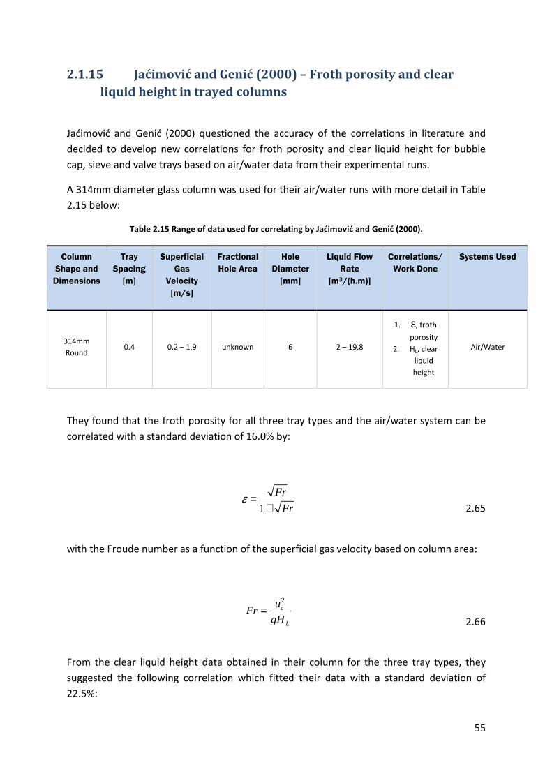
55

2.1.15 Jaćimović and Genić (2000) – Froth porosity and clear

liquid height in trayed columns

Jaćimović and Genić (2000) questioned the accuracy of the correlations in literature and

decided to develop new correlations for froth porosity and clear liquid height for bubble

cap, sieve and valve trays based on air/water data from their experimental runs.

A 314mm diameter glass column was used for their air/water runs with more detail in Table

2.15 below:

Table 2.15 Range of data used for correlating by Jaćimović and Genić (2000).

Column

Shape and

Dimensions

Tray

Spacing

[m]

Superficial

Gas

Velocity

[m/s]

Fractional

Hole Area

Hole

Diameter

[mm]

Liquid Flow

Rate

[m3/(h.m)]

Correlations/

Work Done

Systems Used

314mm

Round 0.4 0.2 – 1.9 unknown 6 2 – 19.8

1. ε, froth

porosity

2. HL, clear

liquid

height

Air/Water

They found that the froth porosity for all three tray types and the air/water system can be

correlated with a standard deviation of 16.0% by:

with the Froude number as a function of the superficial gas velocity based on column area:

From the clear liquid height data obtained in their column for the three tray types, they

suggested the following correlation which fitted their data with a standard deviation of

22.5%:

1

Fr

Frε =

+

2.65

2c

L

uFr

gH=

2.66

56

Since they only tested with an air water system and for limited column geometry Jaćimović

and Genić (2000) suggested that the constants (0.04 and 0.9) in Eq. 2.67 should be

investigated for systems other than air/water and different column geometries. Colwell

(1981) showed that froth porosity (density) and clear liquid height is a function of both the

weir height and the fractional hole area. Since the correlations (Eq. 2.65 and 2.67) proposed

only consider weir height as the column geometrical dependant variable, the applicability of

their correlations for a range of tray and column geometries needs to be investigated.

2.1.16 Van Sinderen et al. (2003) – Entrainment and maximum

vapour flow rate of trays.

Van Sinderen et al. (2003) found that the behaviour of the gas-liquid mixture on trays,

despite all the research done before 2003, is not fully understood. They conducted

entrainment tests in a 0.2 x 0.2m square column with a changeable weir height (0 – 0.3m)

and splash baffle placed above the weir. In their tests they used sieve, fixed valve and valve

trays. The liquid flow rate stayed fixed at 5.04 m3/(h.m) and three gas velocities (ranging

from 1 – 2 m/s, based on column area). They only used one tray and the effect of

entrainment from a “bottom” tray is therefore not accounted for. Their entrainment

measurements were limited to a maximum of 4.8% (entrained liquid per liquid exiting the

downcomer) for the given flow rate. A summary of the test ranges used by Van Sinderen et

al. is shown in Table 2.16 below:

( )0.04 0.9 l l

L wg g

VH H

V

ρρ

= +

2.67

57

Table 2.16 Range of data used for correlating by Van Sinderen et al. (2003).

Column

Shape and

Dimensions

Tray

Spacing

[m]

Superficial

Gas

Velocity

[m/s]

Fractional

Hole Area

Hole

Diameter

[mm]

Liquid Flow

Rate

[m3/(h.m)]

Correlations/

Work Done

Systems Used

0.2 x 0.2m

Square

`0.25 –

0.45

this refers

to

collection

tray

1 – 2 0.06 &

0.076 6 & 12 fixed at 5.04

1. HL, clear

liquid

height

Air/Water

Compared Data

with that of Sakata

and Yanagi (1979)

Van Sinderen et al. (2003) used an inclined mesh pad (see Figure 2.8) with a rectangular

discharge cutter to capture and measure the entrained liquid. They found that the position

of the mesh pad above the tray greatly contributes to the amount of entrainment collected.

Since their inclined mesh pad is not parallel with the test tray and the froth layer above the

tray, the representativeness of their entrainment measurements are therefore questioned.

This also differs from commercial tray columns where the trays are placed parallel above

each other. When they compared their data with those of Sakata and Yanagi (1979, 1982)

they found some discrepancies which they suggest is due to the difference in column scale.

The more logic suggestion would be to investigate the influence of their entrainment

collection system.

Figure 2.8 Section view of the experimental setup used by Sinderen et al. (2003).

Test TrayMoveable

Weir

Froth

Layer

Mesh Pad as

Entrainment

Collector

Entrainment

Collection

Gutter

Splash

Baffle

58

The structure of the froth was redefined in terms of three layers, a bottom layer, middle

layer and a top layer. In the bottom layer bubbles or jets are formed at the holes in the tray

which in turn determines the size of the bubbles or jets. The velocity used to characterise

the bottom layer is the hole gas velocity. The middle layer is formed by erupting bubbles

which create droplets that are projected into the top layer. The velocity of rising bubbles

characterise this layer and was found to be between 0.3 – 1m/s. In the top layer drops are

found. These drops reached vertical heights of 0.05 – 0.5m with horizontal distances, caused

by liquid horizontal momentum, ranging between 0.1 – 0.3m. They found the velocity of the

ejecting droplets to be between 1 and 2m/s.

Not all three layers were always found to be present. They defined two regimes, namely,

the low-liquid-height and the high-liquid-height regimes. In the low-liquid-height regime the

middle layer is absent and was found at low weir heights. By increasing the weir height and

therefore increasing the clear liquid height (liquid hold-up) they found the amount of liquid

entrained into the vapour space above the tray to decrease. In this regime entrainment

depended on tray geometry and tray type. As the liquid height is increased further a

transition was found as the middle layer began to form. At the transition the amount of

liquid entrained into the vapour space was found to be a minimum. By further increasing

the liquid height the amount of liquid entrained will increase and entrainment is

independent of tray geometry and tray type. This is not in agreement with the findings of

Hunt et al. (1955), Kister and Haas (1988) and Bennett et al. (1995) who found entrainment

to be dependent on column and tray geometry in both the froth and spray regimes. Even

though Van Sinderen et al. (2003) do not relate their low – and – high-liquid-height regimes

to the “commonly” known froth and spray regimes, the test ranges used correspond to

those of the previously mentioned authors except at weir heights exceeding 76mm (which is

supposedly high enough for the high-liquid-height regime to exist).

Van Sinderen et al. proposed the following entrainment prediction correlation for the high-

liquid-height regime and all three tray types:

Their definition for both the low – and – high-liquid-layer regimes are the same (HL<HL,tr),

defined as the condition where the clear liquid height is smaller than the clear liquid height

at the regime transition. This is confusing and it is assumed, based on their description of

the regimes, that this is a type error and that the high-liquid-height layer is found where

HL>HL,tr. In order to calculate both the clear liquid height and the clear liquid height at the

regime transition the gas fraction of bubbles in the liquid layer and liquid volume fraction in

( )2130'

0.029 0.01 exp 4.38 2 0.7 17pW p

l p

CLg S H C

A gρ

= ± − − + −

2.68

59

the plane of droplet origin is required. They did not specify how these parameters are

calculated from known system parameters like tray geometry and gas and liquid flow rates.

Based on the work done by Van Sinderen et al. (2003) the influence of the liquid flow rate

on entrainment and the froth behaviour is questioned. They mention that both the weir

height and the liquid flow rate will increase the liquid hold-up which is responsible for the

different regimes and the rate of entrainment. However, the while the liquid flow rate

increases both the liquid hold-up and the liquid horizontal momentum increases. It is the

effect of liquid momentum on froth behaviour and entrainment that needs to be

investigated so that both effects can be determined and accounted for in correlating the

data. Since they only used an air/water system during their tests the influence of gas and

liquid physical properties was not investigated.

2.2 Critical evaluation

In the literature review it was found that the mechanisms and the extent to which they

affect entrainment differ between the froth and spray regimes. All the latest regime (layers

in the case of Van Sinderen et al. (2003)) prediction correlations (Bennett et al. (1995) and

Van Sinderen et al. (2003)) relate the clear liquid height (also referred to as liquid hold-up)

to the transition between the froth and spray regimes. It was found that the liquid hold-up

directly affects the entrainment rate (Hunt et al. (1955), Kister and Haas (1988), Bennett et

al. (1995), and Van Sinderen et al. (2003)).

Colwell (1981) found that the liquid hold-up in the froth regime depends strongly on gas

velocity, liquid flow rate, gas and liquid density, fractional hole area and weir height. This

agrees with the findings of Bennett et al. (1995) even though the latter correlated the

influence of these parameters differently. Due to the complexity of their correlations it is

difficult to compare the differences in the correlations proposed by Colwell (1981) and

Bennett et al. (1995) directly. The advantage of the correlation developed by Bennett et al.

(1995) over that of Colwell (1981) is that no iteration of the liquid hold-up is required.

Each author (Hunt et al. (1955), Thomas and Ogboja (1978), Kister and Haas (1988) and

Bennett et al. (1995)) found different complex relationships between the system

parameters (gas velocity, liquid flow rate and gas and liquid physical properties), tray and

column geometry and entrainment. It is therefore difficult and in most cases impossible to

directly compare the influences of these parameters on entrainment between the various

authors. To show how the different correlations compare (see Table 2.17 and Table 2.18),

they are plotted against each other for a range of gas velocities, liquid flow rates and tray

spacings (see Figure 2.10, Figure 2.11 and Figure 2.12) based on the ranges used by most of

the authors. Hunt et al. (1955) did not test with liquid cross flow, but used clear liquid

60

height in their correlation. Kister and Haas (1988) used the clear liquid height correlation (Eq. 2.23) from Colwell (1981), (see Eq. 2.26) to

calculate entrainment with the correlation of Hunt et al. (1955). Both entrainment correlations from Hunt et al. (1955) and Kister and Haas

(1988) are based on clear liquid height. It was therefore decided to use the clear liquid height correlation developed by Colwell (1981) for

both the Hunt et al. (1955) and Kister and Haas (1988) entrainment correlations in the comparisons shown in Figure 2.10, Figure 2.11 and

Figure 2.12.

Table 2.17 Application range summary of entrainment predictive correlations from literature.

Author

Column

Shape and

Dimensions

Tray

Spacing

[m]

Gas

Superficial

Velocity

[m/s]

Fractional

Hole Area

Hole

Diameter

[mm]

Liquid

Flow Rate

[m3/(h.m)]

Entrainment Correlation/s Systems Used

Hu

nt

et

al.

(1

95

5)

0.152m

Round

0.2 –

0.711 1.0 – 4.3 m/s 0.05 – 0.215 3.18 – 12.7

No liquid

cross flow

Short-comings:

1. No liquid cross flow.

2. Single tray measurements.

3.2*

* *

730.22

2.5s

L

uE

S hσ = −

Eq. 2.2

Methane/Water,

Freon 12/Water,

Air/Kerosene,

Air/Hexane,

Air/CCl4,

Air/water &

glycerine

61


Author

Column

Shape and

Dimensions

Tray

Spacing

[m]

Gas

Superficial

Velocity

[m/s]

Fractional

Hole Area

Hole

Diameter

[mm]

Liquid

Flow Rate

[m3/(h.m)]


Th

om

as

& O

gb

oja

(1

97

8) 0.3 x 0.91m

Rectangular

0.3 –

0.457 1.9 – 3.2

0.124

25.4 4.5 – 40.3

Short-comings:

1. Questionable catch pot entrainment measuring device.

2. Single tray measurements.

3. Influence of fractional hole area on entrainment not incorporated in

correlation.

4. Only air/water system used in tests.

0.77*

* *0.88 p

f

uE

S h

= −

Eq. 2.69

Air/Water

0.81m Round 0.118

62


Author

Column

Shape and

Dimensions

Tray

Spacing

[m]

Gas

Superficial

Velocity

[m/s]

Fractional

Hole Area

Hole

Diameter

[mm]

Liquid

Flow Rate

[m3/(h.m)]


Kis

ter

& H

aa

s (1

98

8)

Used data

from various

sources

0.3 – 1 0.3 – 3.5 0.04 – 0.2 1.5 – 25 2 - 130 Short-comings:

1. Used data from various sources to develop their correlations and can

therefore not account for measurement and/or experimental errors.

2. Empirical correlations are limited to experimental parameter ranges

they were developed from.

3. Applicable to only air/water system.

Advantages:

1. Consider different flow regimes, and tray and column geometry

( )

2

0.5111 1bf H

F

uE d

s hζ

= + −

Eq. 2.38

( )2

2

0.3 Hw

L F

d pE

h s h=

−

Eq. 2.41

( )1.64

10/4 0.25

(10/ ) ,4.742 872 g l gb L cts

L lH

u hE

Qd S

σ

σ ρ ρ ρρ σ

− =

Eq. 2.43Air/Water

63


Author

Column

Shape and

Dimensions

Tray

Spacing

[m]

Gas

Superficial

Velocity

[m/s]

Fractional

Hole Area

Hole

Diameter

[mm]

Liquid

Flow Rate

[m3/(h.m)]


Be

nn

et

et

al.

(1

99

5)

(air

/wa

ter)

Used data

from various

sources

0.15 - 0.91 0.45 – 2.31 0.06 - 0.124 1.6 – 25.4 4.2 – 134

Short-comings:



2. Applicable only to air/water system.

3. Low gas velocities, therefore not considering effect of droplet drag.

Advantages:

1. Semi-empirical correlations, therefore more likely to be accurate when

extrapolated beyond developed parameter range.

1.86 0.51.86 1.852

2

9 30.00164 1 6.9

2s L H L

fe s f L g

K gH DE

g S K A H

ρφ ρ

= + +

Eq. 2.571.26 0.51.26 3.292

2

9 30.0050 1 4.77

2s L H L

se s f L g

K gH DE

g S K A Hβ ρε

φ ρ

= + +

Eq. 2.58

Air/Water

64


Author

Column

Shape and

Dimensions

Tray

Spacing

[m]

Gas

Superficial

Velocity

[m/s]

Fractional

Hole Area

Hole

Diameter

[mm]

Liquid

Flow Rate

[m3/(h.m)]


Be

nn

et

et

al.

(1

99

5)

(no

n-a

ir/w

ate

r)

Used data

from various

sources

0.61 0.07 - 2.41 0.08 - 0.12 12.7 – 25.4 0.25 - 100

Short-comings:

1. Based on data from limited number of systems, mostly under mass

transfer conditions.



3. Low gas velocities, therefore not considering effect of droplet drag.

4. Data from a fixed tray spacing of 0.61m.

1.192.77 1.812

, 20.742 s L L

f NAWe s g

K gHE

g S K

ρφ ρ

=

Eq. 2.707.4

1.56 0.614218

, 2

1.08

2.488 10 1 8.27

s L Hs NAW

e s f L

L

g

K gH DE

g S K A H

β

φ

ρερ

−−

= × + + ×

Eq. 2.71

Non-air/Water

systems nl.:

Cyclohexane/n-

Heptane,

Isobutane/n-

Butane,

Air/Isopar-M oil

65

Table 2.18 Parameter ranges used to compare different entrainment prediction correlations.

System Tray

Spacing

[m]

Superficial

Gas

Velocity

[m/s]

Weir

Height

[mm]

Fractional

Hole Area

Hole

Diameter

[mm]

Liquid Flow

Rate

[m3/(h.m)]

Fs

[(kg/m)1/2/s]

Air/Water @

25°C and

1atm

0.3 – 0.6 1.5 – 3.0 57 0.098 12.7 10 - 60 1.6 – 3.2

The first comparison between the entrainment prediction correlations was made by keeping

the tray spacing and liquid flow rate constant while changing the gas velocity (see Figure

2.9). Entrainment (L’/G) was plotted against the gas superficial velocity.

Figure 2.9. Comparing the effect of gas velocity on entrainment between the different entrainment

prediction correlations. Dotted lines indicate extrapolation beyond recommended range of application.

0%

10%

20%

30%

40%

50%

60%

70%

80%

1.5 2.0 2.5 3.0

En

tra

inm

en

t L

'/G

Gas Velocity [m/s]

Hunt et al.

(1955)

T & O (1978)

K & H (1988)

Bennett et al.

(1995)

QL = 10m3/h.m

S = 457mm

hw = 57mm

Af = 0.098

dH = 12.7mm

ρv = 1.16kg/m3

66

Figure 2.9 shows that at low gas velocities (1.5 – 2m/s) there is no significant difference

between the correlations. However, when the gas velocity exceeds 2m/s the correlations

deviate significantly. Hunt et al. (1955) assumed that the froth density stays constant. Both

Colwell (1981) and Bennett et al. (1995) later showed that froth density is a function of gas

velocity, liquid flow rate, gas and liquid density, and column and tray geometry. The

assumption of constant froth density by Hunt et al. (1955) is therefore an oversimplification.

Kister and Haas (1978) only used the low gas velocity data (0.8 – 1.5m/s) from Thomas and

Ogboja (1978) to develop their prediction correlation even though Thomas and Ogboja

generated entrainment data for gas velocities up to 3.2m/s. One of the reasons for the

deviation in entrainment prediction by Thomas and Ogboja (1978) could be the use of a

catch pot device filled with silica gel to measure entrainment. The effectiveness and

representativeness of such a device that does not cover the total column area is

questionable, particularly at high entrainment rates. Kister and Haas (1988) used a larger

data bank than Hunt et al. (1955) and Thomas and Ogboja (1978) to develop their

correlation and it is therefore expected that their correlation should perform better than

the latter over a large range of operating conditions. However, since they used data from

various sources to develop their empirical entrainment prediction correlation, possible

deviations are expected when operating outside the range of the data used. Systematic

errors caused by poor experimental setup design and measurement errors from the

different experimental setups used to generate data are not accounted for and could also

lead to deviations between predictions and real column operation. Bennett et al. (1995)

developed a semi-empirical correlation to predict entrainment over a large range of

operating and system parameters. It is therefore expected that their correlation should

perform better when extrapolated beyond their recommended application range. Bennett

et al. (1995) did however mention that deviations are to be expected at high gas velocities

due to their assumption that droplet drag will have negligible effect on entrainment at their

proposed low operating gas velocity (<2.31m/s) range.

The next comparison, Figure 2.10, between the correlations was made by changing the

liquid flow rate while keeping the tray spacing and gas velocity constant. The gas velocity

was kept low, 2m/s, since the entrainment prediction between the correlations agreed well

at low gas velocities as shown in Figure 2.9.In this example entrainment will be given as

mass entrained liquid per mass of rising gas (Figure 2.10 (a)) and as mass entrained liquid

per mass of liquid entering the tray (Figure 2.10 (b)).

67

Figure 2.10 Investigating the influence of liquid flow rate on entrainment for the different entrainment

prediction correlations, plotted as (a) mass entrained liquid per mass rising vapour (b) mass entrained liquid

per mass liquid entering the tray under exactly the same conditions. Dotted lines indicate extrapolation

beyond recommended range of application or testing.

0.0%

1.0%

2.0%

3.0%

4.0%

5.0%

0 20 40 60 80

En

tra

inm

en

t L

'/G

QL [m3/(h.m)]

Hunt et al.

(1955)

T & O (1978)

K & H (1988)

Bennett et al.

(1995)

S = 457mm

us = 2m/s

hw = 57mm

Af = 0.098

dH = 12.7mm

ρv = 1.16kg/m3

0.0%

0.2%

0.4%

0.6%

0.8%

1.0%

1.2%

1.4%

1.6%

0 20 40 60 80

En

tra

inm

en

t L

'/L

QL [m3/(h.m)]

Hunt et al.

(1955)

T & O (1978)

K & H (1988)

Bennett et al.

(1995)

S = 457mm

us = 2m/s

hw = 57mm

Af = 0.098

dH = 12.7mm

ρv = 1.16kg/m3

(a)

(b)

68

Figure 2.10 (a) shows that an increase in liquid flow rate will result in an increase in

entrainment (L’/G) in the froth regime as mentioned by Kister and Haas (1988). However,

when entrainment is measured as the mass of liquid entrained over the mass of liquid

entering the tray (L’/L), a different trend is observed (see Figure 2.10 (b)) where

entrainment decreases with increasing liquid flow rate. Figure 2.10 (b) gives a much better

understanding of the influence of the liquid flow rate on the percentage entrainment from

an operating point of view. By relating the entrained liquid with the liquid entering the tray

it is easier to determine the fraction of liquid and their components (in distillation

operation) that is transported with entrainment to the tray above.

The sudden inflexion in the trend by Kister and Haas (1988) in Figure 2.10 (a) is caused by

their anticipation of a regime change from spray to froth. However, according to Bennett et

al. (1995) the flow regime is the froth regime and does not change for the liquid flow rate

range presented. After reinspection of their correlation it was found that the correlation for

regime transition by Kister and Haas (1988) is not accurate. This was found when their

regime correlation was compared to conditions they specified as froth regime (Figure 5 in

Kister and Haas (1988)) and their spray regime entrainment correlation matched the data

while the froth regime correlation deviated significantly. It should be noted that the

correlation for entrainment in the froth regime by Kister and Haas (1988) is only an

adaptation from the Hunt et al. (1955) correlation. At a liquid flow rate of 60 m3/(h.m) the

correlation by Hunt et al. (1955) agrees with that of Bennett et al. (1995). It is interesting to

note that at this specific point the froth density and clear liquid height of Hunt et al. (1955)

is the same as that predicted by Bennett et al. (1995). When entrainment is plotted as the

entrained liquid per liquid entering the tray (Figure 2.10 (b)) the trends follows a very similar

curvature. It should also be noted that the percentage entrainment in both Figure 2.10 (a)

and (b) is very low and the correlations are not extrapolated beyond the recommended

range of application.

The last comparison (Figure 2.11) between the entrainment prediction correlations was

made by changing the tray spacing while maintaining a constant gas and liquid velocity.

69

Figure 2.11 Investigating the influence of tray spacing on entrainment for the different entrainment

prediction correlations. Dotted lines indicate extrapolation beyond recommended range of application or

testing.

Figure 2.11 shows that a decrease in tray spacing will result in an increase in entrainment

under constant froth height conditions. This decrease is not linear which shows that the

froth density is not constant with height above the tray floor. This agrees with the findings

of Hofhuis and Zuiderweg (1979) that the froth density decreases with elevation from the

tray floor. At 300mm tray spacing the correlation from Hunt et al. (1955) agrees with that of

Bennett et al. (1995) at this point however the froth densities predicted by Hunt et al. and

Bennett et al. differed. The prediction by Kister and Haas (1988) shows a much higher

dependency on tray spacing than that of Bennett et al. (1995). The deviation could be due

to the fact that Kister and Haas (1988) develop an empirical correlation while Bennett et al.

(1995) developed a more fundamental (semi-empirical) model. The curvature of the Hunt et

al. (1955) and Kister and Haas (1988) correlations corresponds which shows the influence of

the empirically derived non-uniformity adaptation made by Kister and Haas (1988) to the

Hunt et al. (1955) correlation at low clear liquid heights. Once again the prediction by

Thomas and Ogboja (1978) shows significant deviation from the others.

The graphs in Figure 2.12 (a) and (b) are plotted to show how the froth height correlations

of various authors compare over a range of gas and liquid flow rates.

0.0%

0.5%

1.0%

1.5%

2.0%

2.5%

3.0%

3.5%

4.0%

4.5%

300 350 400 450 500 550 600 650

En

tra

inm

en

t L

'/L

Tray Spacing [mm]

Hunt et al. (1955)

T & O (1978)

K & H (1988)

Bennett et al.

(1995)

QL = 10m3/h.m

us = 1.75m/s

hw = 57mm

Af = 0.098

dH = 12.7mm

70

Figure 2.12 Investigating the influence of (a) gas and (b) liquid flow rate on entrainment for the different

entrainment prediction correlations.

0

50

100

150

200

250

1.0 1.5 2.0 2.5 3.0 3.5

Fro

th H

eig

ht

[mm

]

us [m/s]

T & O (1978)

Colwell (1981)

Bennett et al.

(1995)

QL = 10m3/h.m

S = 457mm

hw = 57mm

0

50

100

150

200

250

300

350

0 20 40 60 80

Fro

th H

eig

ht

[mm

]

QL [m3/(h.m)]

T & O (1978)

Colwell (1981)

Bennett et al.

(1995)

S = 457mm

us = 1.5m/s

hw = 57mm

(a)

(b)

71

Figure 2.12 (a) and (b) shows that an increase in gas velocity and liquid flow rate will result

in an increase in froth height. All the trends follow a similar curvature with Thomas and

Ogboja (1978) predicting the highest froth height. One would therefore expect Thomas and

Ogboja (1978) to over predict entrainment in Figure 2.9 and Figure 2.10. Since this is not the

case it has to be assumed that the accuracy of their entrainment measuring device is

questionable given that they developed an empirical entrainment prediction correlation

from their entrainment data.

2.3 Summary of literature survey

Based on the content covered in the literature review and the critical evaluation the

following summary was made:

Correlations have been developed to:

1. Predict the flow regime of the dispersion above the tray based on system conditions

and tray geometry.

2. Predict the froth height and froth density for mainly air/water systems.

3. Predict entrainment in both the froth and spray regime for mainly air/water systems.

Entrainment prediction correlations developed for non-air/water systems were

developed based on limited data with questionable reliability.

4. Determine the tray pressure drop as a function of the residual and dynamic pressure

drop, and momentum heads at the sieve tray holes.

Figure 2.9 - Figure 2.12 compared the different entrainment and froth height prediction

correlations with each other. The largest deviations between the entrainment prediction

correlations of the various authors were found at higher (>2 m/s) superficial gas velocity. At

low liquid rates and low tray spacing the correlations also tend to differ significantly with

the entrainment prediction correlation from Thomas and Ogboja (1978) which showed the

largest deviation when compared to trends of the other correlations. Most of the variations

between the trends are caused by the limited range (gas and liquid flow rates, gas and liquid

physical properties) of testing and in some cases poor experimental setup design. The

variation between the trends in Figure 2.9 - Figure 2.11 is proof that more work is required

to improve understanding of the mechanisms that affect entrainment. In order to

investigate these mechanisms a large range of gas and liquid flow rates, gas and liquid

physical properties, and, tray and column geometry should be investigated in a single

experimental setup. This will eliminate systematic errors caused by experimental setup

design and different sampling methods.

72

Very little reliable non-air/water data exists compared to the work done with air/water

systems. The correlations developed by Kister (1990) and Bennett et al. (1995) are based on

data generated from different column geometries and from different experimental setups.

It is unclear how accurate and representative the data is since limited information is given

regarding the collection of the data. Sakata and Yanagi (1979) acknowledged that they

experienced difficulties measuring entrainment. Most of the non-air/water correlations are

based on the data from Sakata and Yanagi (1979).

In the publications reviewed the definition for the different flow regimes varied between

the different authors. Porter and Jenkins (1979) related the froth to spray transition to the

minimum entrainment that is achieved when the liquid flow rate is increased while the

vapour velocity is kept constant. This related the tray capacity to the respective regime. The

only problem is that their definition for the entrainment rate (ratio of the mass entrained

liquid to the mass of vapour) does not relate to the amount of liquid on the tray. The effect

of entrainment on the concentration of the high and low volatile components in the liquid

phase on the tray is therefore not considered.

All the authors defined entrainment as the mass of liquid entrained over the mass of rising

vapour or as the amount of entrained liquid that reached the entrainment collection

section. Therefore ten percent entrainment for a fixed gas flow rate is the same amount of

liquid entrained irrespective of the liquid flow rate. This is better explained in the following

example (see Figure 2.10 (a) and (b)):

If for a constant vapour flow rate of 1 kg/s and a liquid flow rate of 1 kg/s an entrainment

rate of 100% is reached all the liquid on the tray (1kg/s liquid) will be moved from the tray

below to the tray above. In the case where the liquid flow rate is 10 kg/s with a 1 kg/s

vapour flow rate, 100% entrainment rate is still 1 kg/s liquid that are moved to the tray

above. The significant difference is that 1 kg/s in this case is only 10% of the total liquid flow

rate entering the tray and would therefore not influence the mass transfer efficiency to the

extent as when all the liquid is moved from the tray below to the tray above. The definition

of entrainment is therefore not related to the amount of liquid on the tray and can

therefore not be directly linked with the mass transfer separation efficiency.

Most of the correlations developed to predict froth height and entrainment assumes that

the effect of droplet drag can be neglected. Bennett et al. (1995) showed that at high

superficial vapour velocities and for high Froude and Weber numbers droplet drag does

have a significant influence on entrainment. The effect of liquid viscosity on the

hydrodynamic behaviour has not been focused on. Most of the work done on the influence

of viscosity on entrainment used a small range (0.8 – 2 mPa.s) of viscosities. No entrainment

predicting correlation has been developed that can accurately predict entrainment for

air/water and non-air/water systems over a broad operating range.

73

2.4 Scope for potential research

Based on the summary made of the literature review, the following areas in sieve tray

hydrodynamics require investigation:

1. The influence of a large range of gas and liquid physical properties, with fixed tray

geometry, on:

i. the clear liquid height (liquid hold-up);

ii. froth density;

iii. entrainment at different tray spacings to investigate the influence of droplet

drag for low surface tension liquids;

iv. weeping

2. The influence of the liquid flow rate on entrainment and froth behaviour at fixed

clear liquid heights (liquid hold-up).

3. The minimum entrainment, for a range of system physical properties, as a function

of liquid entering the tray through the downcomer.

Most of the deviations found between the entrainment prediction trends of the various

authors (in Figure 2.9 - Figure 2.11) and others (Van Sinderen et al. (2003)) can be related to

poor experimental setup design and sampling methods. Therefore, in order to achieve the

above it is of utmost importance to spend time on the design of an experimental setup to

ensure representative and accurate results.

2.4.1 Scope for this work

The aim for this project was therefore to develop an experimental setup to investigate

hydrodynamic behaviour in sieve tray columns while isolating the effects of mass transfer

which occurs in commercial distillation. An overview of the different column geometries

used in the past by different research groups with their findings acted as a guide to

approach the optimum column design. Some advice and suggestions regarding column and

tray geometry were proposed by Koch – Glitsch (international tray and packing supplier and

developer).

To verify system accuracy and representativeness air/water tests were conducted and the

results compared with entrainment prediction correlations from Hunt et al. (1955), Thomas

and Ogboja (1978), Kister and Haas (1988) and Bennett et al. (1995).

74

3 Design of a distillation sieve tray column for

hydrodynamic characterisation

3.1 Introduction

In order to generate entrainment data with non-mass transfer systems an experimental

setup had to be designed. Different column geometries have been used in the past to

generate data representing the hydrodynamic behaviour in sieve tray columns. Table 2.17 is

a summary of the column geometries previously used by different research groups.

Hunt et al. (1955) found that the liquid flowing over the weirs in a small diameter round

column is unstable and therefore conducted their studies with no liquid cross flow. Porter

and Jenkins (1979) showed that round columns will have a constriction effect on the cross

flowing liquid at the outlet weir. The sudden expansion in the liquid flow path, after exiting

the downcomer, could also contribute to non-uniform froth development. It was therefore

decided to use a column with rectangular shape to eliminate entrance and wall effects. To

eliminate a possible effect of mass transfer on entrainment, and to focus on hydrodynamic

behaviour, it was decided to design the pilot plant for thermally stable non-reacting, and

non-foaming, gas and liquid systems. By using a zero mass transfer system, the gas and

liquid flow rate measurements will be simplified compared to industrial distillation where

the composition of the components and flow rate of the phases and fractions change

throughout the column.

3.1.1 Objective

The objective of this section is to describe the development of an experimental setup that

would allow generation of reliable entrainment data for:

1. a range of gasses with different densities;

2. a range of liquids with different;

a. Densities

b. Viscosities

c. Surface tensions

3. different tray spacings;

4. a range of gas and liquid flow rates.

It was decided that the experimental setup should also be able to measure weeping rates

even though it does not fall within the scope of this project.

75

3.1.2 Scope and Limitations

The following is a summary of the limitations that determined the scope for constructing the

experimental setup:

1. Time

2. Laboratory Space

3. Gas and liquid systems

4. Gas and liquid flow rates

5. Materials for Construction

6. Safety

Time:

Construction and commissioning of the experimental setup is limited to two years since a

year is needed for testing with an air/water system, generating entrainment data and

reporting the findings.

Laboratory space:

Space for the development of an experimental setup was limited. The experimental setup

could not exceed a height of 8m and only 20m2 of floor space was available. The available

space had to be shared with another column (that will be used to investigate the

hydrodynamic behaviour for structured and random packing) that will make use of the same

utilities as this experimental setup.

Gas and liquid systems:

The aim was to generate data that represents a large fraction of the systems used in

distillation, absorption and stripping applications. Since one of the objectives is to eliminate

the possible influence of mass transfer on the hydrodynamic behaviour, care was taken with

the selection of the liquid systems. If the flash point is low and or the vapour pressure high,

evaporation will take place which would include the effect of mass transfer on the

measurements. Flammable liquid in the vapour phase will also increase the risk of fire and

explosion.

Since it is expensive and nearly impossible to create gas mixtures of known concentration in

such a large system it was decided to use pure (technical grade) gasses. To reduce the

possibility of air leakage into the system, especially at the blower shaft seal, the operating

pressure should be slightly above atmospheric pressure. Air that leaks into the system when

using a flammable liquid will increase the probability of fire and an explosion.

76

The range of liquid and gas systems therefore depended on the availability, cost, corrosive

properties and safety.

Gas and liquid flow rates:

According to the entrainment rate (ratio of liquid entrained over liquid entering the tray)

prediction correlation of Bennett et al. (1995) for the froth regime a superficial gas velocity

of 5.4 m/s is required to achieve 20% entrainment for a liquid rate of 120 m3/(h.m). Since

the exact superficial velocity required for excessive entrainment is uncertain (the superficial

velocity exceeds the range, 0.5 - 2.3m/s, used by Bennett et al. (1995)) a maximum velocity

of 7 m/s was chosen (this velocity had to be excessive since the required velocity for

entrainment for Helium gas is uncertain).

The correlation developed by Bennett et al. (1995) covered a liquid range of 4.18 – 134.28

m3/(h.m). It was therefore decided to test for a liquid range of 11 – 114 m

3/(h.m) since more

than one flow meter would be required for a larger flow range. This flow range should be

sufficient to test the influence of excessive entrainment for high liquid rates. The liquid flow

rate is based on the volumetric flow rate per weir length.

Materials for construction:

Organic solvents are known for their corrosive properties on seals and polymeric

compounds. PTFE (polytetrafluoroethylene) or Viton (a fluoropolymer elastomer) seals were

therefore used. Due to the corrosiveness of the organic solvents glass should be used for

viewing ports. Polycarbonate (LEXAN) was used as viewing ports since glass would tend to

crack and create sealing problems.

Water will be used therefore the construction material should be stainless steel, grade 304

or 316.

Safety:

With the use of flammable liquids and gasses special rules and legislation apply. Based on

the MSDS (material safety data sheet) properties and the operating conditions, precautions

regarding sensor and electronic device selection and placement have to be made. Since the

safety legislation was not the aim of the study an in depth investigation of the rules and

legislation will not be covered in this work.

To ensure safe operation a proper HAZOP (Hazard and Operability Study) was conducted. In

order to reduce the probability of fire and explosions, contact with air should be eliminated

by maintaining a system pressure greater than the atmospheric pressure, the area should be

well ventilated and the system should be free of gas and liquid leaks.

77

3.2 Concept design

3.2.1 Pilot Plant Unit Selection

The pilot plant will need the following main units:

1. The distillation hydrodynamic characterisation sieve tray column.

2. A blower to circulate the gas (since no re-boiler will be used).

3. A pump to circulate the liquid (since no condenser will be used).

4. Vessels than can measure the entrainment and weeping rates.

5. A surge tank that will act as a dampener to possible system pressure fluctuations.

This vessel should also act as a droplet settling tank to remove and measure

droplets which can be carried over with the gas from the de-entrainment section

of the column.

6. Heat exchanger to control the operating temperature.

7. Sensors that will measure flow rate, absolute pressure, pressure drop, and

temperature.

8. Control system to control temperature, flow rate and pressure.

9. A catwalk structure to make visual observation, manual settings, sampling and

maintenance possible.

3.2.2 Pilot plant layout

The process flow diagram in Figure 3.1 represents the schematic layout of the plant. The

function of each unit will be discussed in section 3.3 with the detailed specifications in

Appendix A (section 8).

Liquid circulation loop:

Liquid is circulated from the sump with a centrifugal pump through a flow meter and control

valve to the heat exchanger where excess process heat is removed. From the heat

exchanger the liquid is fed into the downcomer above test tray 1 of the column. As the

liquid enters test tray 1, it is brought in contact with the rising gas. In the event where no

entrainment occurs, all the liquid will exit test tray 1 and enter test tray 2. The main purpose

of test tray 2 is to cool and distribute the gas coming from the blower as well as to represent

flow conditions found in multi tray columns. The liquid will then exit test tray 2 through a

downcomer, which is isolated from the chimney tray section, to the sump. Alternatively the

78

liquid can be circulated from the heat exchanger through the sump, bypassing the trays and

any gas contact.

During entrainment conditions the gas velocity is sufficiently high to transport the liquid on

test tray 1 to the de-entrainment section. The entrained liquid is then removed from the

rising gas stream and fed through MV-204 to the sump. To determine the rate of

entrainment the valve below MV-204 will be closed (low entrainment rates) or the

entrained liquid will be fed to MV-202 (high entrainment rates). The mass inside either MV-

202 or MV-204 is then logged over time to determine the rate of entrainment.

Figure 3.1 Schematic representation of the pilot plant setup.

Venturi

P

Sump

Ma

ss f

low

me

ter

79

Weeping occurs when the gas velocity is sufficiently low for the liquid to ‘leak or dump’

through the perforations in the tray to the chimney tray. The chimney tray is sealed so that

no liquid on the tray can leak through to the sump. The ‘chimneys’ or gas distributors are

elevated above the tray deck to prevent gas-liquid contact. The liquid exits the chimney tray

section through a 3-way valve to either the sump or MV-203 which will measure the

weeping rate over time.

To evacuate MV-202 or MV-203 valves are switched so that the pump is no longer fed from

the sump. As soon as MV-202 or MV-203 is emptied the valves will switch back so that the

pump is fed from the sump.

Gas circulation loop:

Gas is fed to the column by a centrifugal blower through a gas distributor, shown as the

chimney tray in Figure 3.1. The gas will then rise through the column exiting through a

venturi meter to a surge tank. The surge tank absorbs pressure fluctuations as well as

separates any remaining liquid droplets from the gas. From the surge tank the gas is fed to

the blower completing a closed loop.

3.3 Detail design

3.3.1 Choosing gas and liquid systems

In order to conduct sensor, unit, and pipe sizing, the range of gas and liquid physical

properties that will be used to generate the required data were needed. To generate data

that represents a large fraction of the systems found in commercial distillation applications

it was decided to look at the physical properties of a range of hydrocarbons around their

boiling points (at saturation). The physical properties of the gas and liquid systems should

compare to a hydrocarbon range of C1 – C12 (methane to dodecane) to represent the

physical properties of most systems used in commercial distillation, as shown in Table 3.1.

This range was also selected based on the molecular mass range (16 – 170 kg/kmol) which

covers most systems used in commercial distillation. The objective for the design includes

that it should be able to test the influence of a range of gas and liquid physical properties on

entrainment. In stripping applications where volatile components are removed from waste

water or in the case where some polymers might be present in the liquid, the viscosity and

surface tension range had to be increased beyond distillation applications. The effect of

foaming on the hydrodynamic behaviour does not form part of this investigation and will

therefore not be investigated.

80

Table 3.1 Vapour/liquid physical properties found in commercial stripping and distillation applications

obtained from www.nist.gov.

Description Chemical

Formula

Mr

[kg/kmol]

Temp

[°C]

Absolute

Pressure

[kPa]

Liquid

density

[kg/m3]

Vapour

Density

[kg/m3]

Liquid

Viscosity

[mPa.s]

Surface

tension

[mN/m]

Methane CH4 16 -162 100 422 1.8 0.12 13

Butane C4H10 58 -0.8 100 602 2.7 0.20 15

Pentane C5H12 72 36 100 610 2.9 0.20 14

Octane C8H18 114 125 100 612 3.7 0.20 12

Decane C10H22 142 174 100 604 4.1 0.20 11

Dodecane C12H26 170 216 100 595 4.5 0.20 9

Oxygen O2 32 -183 100 1142 4.4 0.20 13

Oxygen O2 32 -153 1000 976 38.5 0.10 6

Cyclohexane C6H12 84 80. 100 720 2.97 N/A 18

Water H2O 18 100 100 958 0.59 0.28 59

Water H2O 18 20 2.3 998 0.017 1.00 73

Water H2O 18 25 3.2 997 0.023 0.89 72

Ethylene

Glycol C2H6O2 62 25 100 1113 N/A 15.00 48

Since the aim of this investigation is to study entrainment (hydrodynamics) and not

thermodynamics, the liquids which will be used for testing should have a low saturated

vapour pressure to prevent evaporation at 25°C (the chosen operating temperature). At

25°C no excessive cooling or heating is required for temperature control. The gas/liquid

range is also limited to availability, cost and safety. Most of the work done in the literature

focused on the gas and liquid densities, future work will focus on a large range of liquid

surface tensions and especially a large range of liquid viscosities to represent commercial

distillation and stripping applications. Table 3.2 and Table 3.3 is a summary of the chosen

gasses and liquids with their properties. The values are only approximations and will be

analytically verified and measured during and after testing.

81

Table 3.2 Approximated Gas Properties (obtained from www.nist.gov).

Gas Mr

[kg/kmol]

Density

[kg/m3]

Dynamic

Viscosity

[mPa.s]

Kinematic

Viscosity

[m2/s]

He 4 0.16 1.98E-02 1.24E-04

Air 29 1.18 1.82E-02 1.54E-05

CO2 44 1.78 1.49E-02 8.37E-06

SF6 146 5.96 1.53E-02 2.56E-06

Table 3.3 Approximated Liquid Properties (obtained from www.nist.gov).

Liquids Mr

[kg/kmol]

Density

[kg/m3]

Dynamic

Viscosity

[mPa.s]

Surface

Tension

[mN/m]

Boiling

Point @

1 atm [°C]

Water 18 997 0.89 73 100

Ethylene Glycol 62 1113 15.4 48 198

Silicone Oil 74 963 50 19 130

n-Butanol 74 810 2.6 24.9 118

Isopar G not specified 748 0.84 23.1 160

The gas density range cover the vapour density range found in most commercial

applications. The liquid density range does, however, not cover the low liquid densities

found in commercial applications. However, the liquid density range is large enough so that

the effect of liquid density on entrainment can be determined and extrapolated to lower

density liquid applications. The liquids also cover a large surface tension and viscosity range

which was not previously tested for by other research groups.

82

3.3.2 Column design

The main column design was proposed by Koch-Glitsch and modified to meet the

requirements of this project. The gas enters at the bottom of the column through a gas

distributor that also acts as the weeping collection tray. Above the weeping collection tray,

two test trays are followed by a de-entrainment tray and a mist eliminator pad, see Figure

3.1. The liquid enters the column through a sealed downcomer placed in the de-

entrainment section. This ensures that the liquid rate entering the tray can be measured

and are representative of real column operation. Some changes and adjustments, regarding

tray spacing and the viewing ports, were then made to meet the objectives.

The following was considered in the design of the column:

1. The column shape

2. Tray spacing

3. Tray geometry

4. Visibility

5. Downcomer clearance area (downcomer escape area)

6. De-entrainment section

7. Weeping collection section

8. Liquid sump

Column shape:

The column shape was chosen to be rectangular to eliminate possible entrance (expansion),

exit (constriction) and wall effects of the liquid flow path on the hydrodynamics in the

column associated with small to medium size round columns. The column size was chosen

to be 175 x 635mm. Koch-Glitsch provided the de-entrainment and mist eliminator devices,

the test trays and the gas distributor. Figure 3.2 and Figure 3.3 are detailed drawings of the

column with some dimensions.

Figure 3.2 Column front view with dimensions in millimetres.Column front view with dimensions in millimetres.

83

Figure 3.3 Column sideColumn side-and-isometric views with dimensions in millimetres.

84

with dimensions in millimetres.

85

Tray spacing:

It was decided to use two trays in order to represent the hydrodynamic behaviour of a

multi-tray distillation column. The hydrodynamic effect that the bottom tray has on the top

tray during entrainment will therefore be included in the test results.

Most of the work done in the literature was for a tray spacing range between 300 and

600mm. It was therefore decided to design the column to accommodate 4 tray spacings;

315, 415, 515 and 615mm. In order to change the tray spacing separate sections had to be

constructed. This influenced the piping that connects the gas and liquid lines to the column.

Tray geometry information:

Table 3.4 is a summary of the test tray geometry:

Table 3.4 Sieve Tray and Column Geometry.

Variable Description Value

Ab [m2] Bubbling Area 0.0796

Ad [m2] Downcomer Area 0.0158

Af [m2] Fractional hole area 0.155

Ah [m2] Hole area 0.0143

Ap [m2] Perforated Area 0.0919

Number of Holes

(including bubble promoters)

458

dH [mm] Hole diameter 6.3

hw [mm] Weir height 57

l [mm] weir length 175

p [mm] Hole triangular pitch 14

s [mm] Tray spacing 615

Figure 3.4 is a picture of the sieve trays used in this work:

Figure

Visibility:

Since the aim of this investigation is to characterise the hydrodynamic behaviour inside the

column, visual observation is needed to monitor:

1. When entrainment and weeping occur.

2. The froth development

3. If the downcomer is flooding

4. If there is sufficient liquid in the downcomer (

bypass through the downcomer

5. If the de-entrainment section is flooding or at maximum capacity

6. If the weeping section is at maximum capacity.

Glass or transparent sections are therefore needed in the column walls to create

The challenge is therefore to design and construct window frames that seal and allow the

glass to be removed to allow access to the column internals from the outside. The glass

should be flush with the inside of the column wall to retain a smoo

path.

Downcomer clearance area:

The downcomer clearance (escape) area should be adjustable to:

1. Prevent the downcomer from flooding (downcomer flooding occurs when the

downcomer is overfilled with liquid preventing the liquid from the

exit).

picture of the sieve trays used in this work:

Figure 3.4 Picture of a sieve tray used in this work.

nvestigation is to characterise the hydrodynamic behaviour inside the

column, visual observation is needed to monitor:

When entrainment and weeping occur.

The froth development.

If the downcomer is flooding.

If there is sufficient liquid in the downcomer (downcomer seal) to prevent gas

bypass through the downcomer.

entrainment section is flooding or at maximum capacity

If the weeping section is at maximum capacity.

Glass or transparent sections are therefore needed in the column walls to create



should be flush with the inside of the column wall to retain a smooth gas and liquid flow

The downcomer clearance (escape) area should be adjustable to:

Prevent the downcomer from flooding (downcomer flooding occurs when the

downcomer is overfilled with liquid preventing the liquid from the

86

nvestigation is to characterise the hydrodynamic behaviour inside the

downcomer seal) to prevent gas

entrainment section is flooding or at maximum capacity

Glass or transparent sections are therefore needed in the column walls to create visibility.



th gas and liquid flow

Prevent the downcomer from flooding (downcomer flooding occurs when the

downcomer is overfilled with liquid preventing the liquid from the tray above to

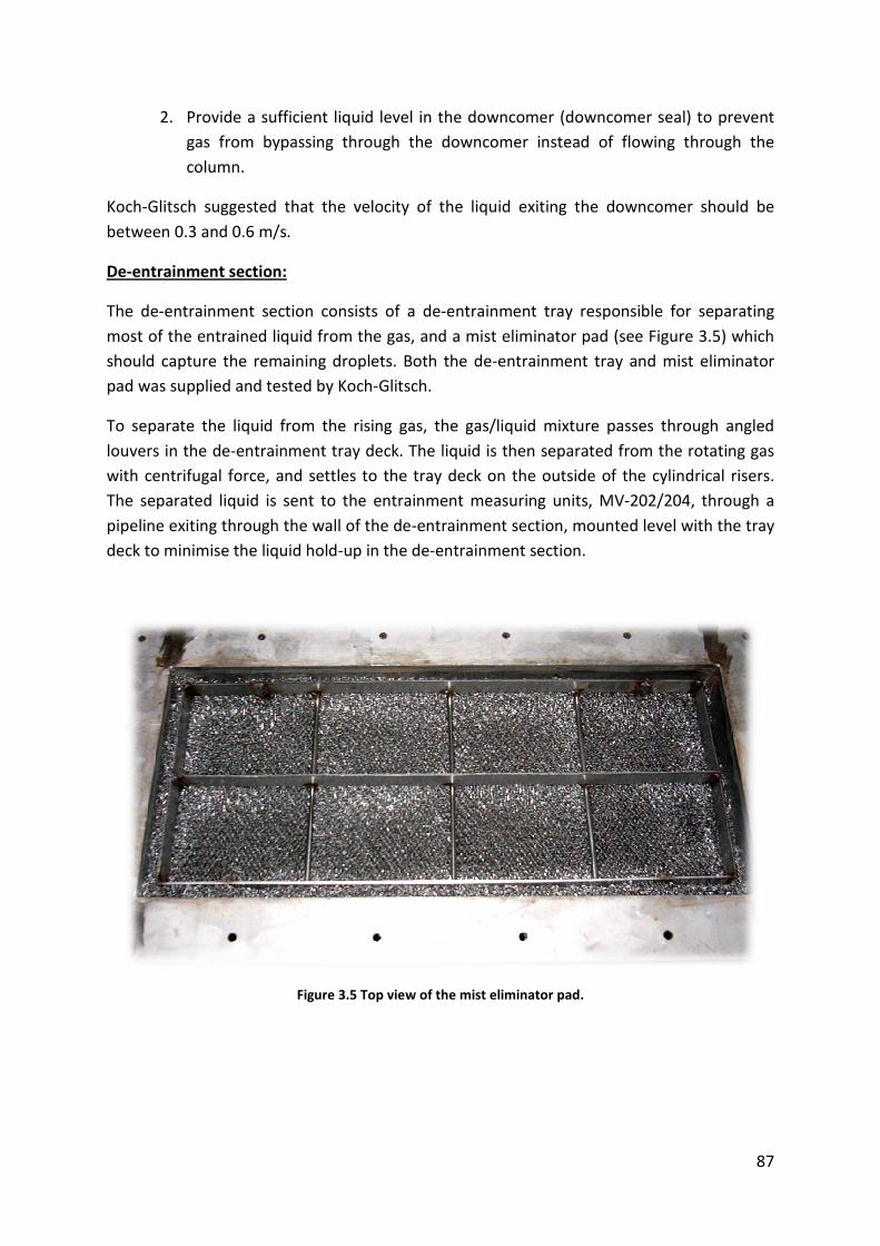
2. Provide a sufficient liquid level in the downcomer (downcomer seal) to prevent

gas from bypassing through the downcomer

column.

Koch-Glitsch suggested that the velocity of the liquid exiting the downcome

between 0.3 and 0.6 m/s.

De-entrainment section:

The de-entrainment section consists of a de

most of the entrained liquid from the gas, and a mist eliminator pad

should capture the remaining droplets. Both the de

pad was supplied and tested by Koch

To separate the liquid from the rising

louvers in the de-entrainment

with centrifugal force, and settles to the tray deck on the outside of the cylindrical risers.

The separated liquid is sent to the entrainment measuring units

pipeline exiting through the wall of the de

deck to minimise the liquid hold

Figure

Provide a sufficient liquid level in the downcomer (downcomer seal) to prevent

gas from bypassing through the downcomer instead of flowing through the

Glitsch suggested that the velocity of the liquid exiting the downcome

entrainment section consists of a de-entrainment tray responsible for separating

most of the entrained liquid from the gas, and a mist eliminator pad (see

should capture the remaining droplets. Both the de-entrainment tray and mist eliminator

pad was supplied and tested by Koch-Glitsch.

e the liquid from the rising gas, the gas/liquid mixture passes through angled

entrainment tray deck. The liquid is then separated from the rotating gas

centrifugal force, and settles to the tray deck on the outside of the cylindrical risers.

sent to the entrainment measuring units, MV-20

pipeline exiting through the wall of the de-entrainment section, mounted level with the tray

deck to minimise the liquid hold-up in the de-entrainment section.

Figure 3.5 Top view of the mist eliminator pad.

87

Provide a sufficient liquid level in the downcomer (downcomer seal) to prevent

instead of flowing through the

Glitsch suggested that the velocity of the liquid exiting the downcomer should be

responsible for separating

(see Figure 3.5) which

entrainment tray and mist eliminator

the gas/liquid mixture passes through angled

ated from the rotating gas

centrifugal force, and settles to the tray deck on the outside of the cylindrical risers.

202/204, through a

entrainment section, mounted level with the tray

88

Weeping collection section:

The weeping collection tray, designed and supplied by Koch-Glitsch, acts as a gas distributor

and a weeping collection tray. The tray consists of “chimneys” protruding the tray deck

(approximately 250mm) which act as gas distributors. The liquid that weeps through the

bottom test tray is therefore collected on the tray deck and fed to the weeping measuring

vessel, MV-203. A sealed downcomer is used to transport the liquid exiting test tray 2 to the

liquid sump to ensure isolation of the weeping collection section.

Liquid sump:

The liquid sump was elevated to supply a net positive suction head (NPSH) of 6.5m (64kPa)

to the pump. Since the liquid entering the sump form test tray 2 contains entrained gas

bubbles a splash deck was placed at the bottom of the downcomer to redirect the liquid

flow path so that the bubbles have sufficient time to disengage from the liquid. A vortex

breaker was placed inside the exit pipe feeding the pump to prevent the formation of a

vortex that will cause the pump to suck gas into the pipeline and cause cavitation.

3.3.3 Gas blower (E-102)

It was chosen to use a centrifugal blower to circulate the gas through the pilot plant. After

the pressure drop calculations for the gas line (piping, fittings and column) were completed

the design specifications as shown in Table 8.1 in Appendix A were sent to the supplier.

The blower was placed in an acoustic enclosure outside the laboratory to reduce noise

levels. A plinth was specially designed and constructed to support the blower with the

acoustic enclosure. To further ensure flexible operation of the blower, especially at low

volumetric flow rates, an inverter was connected to the blower that controls the rotational

speed and therefore the gas flow rate.

3.3.4 Liquid pump (E-204)

Since the pressure required to circulate the liquid through the liquid pipeline, heat

exchanger and column, is below 10 bar a centrifugal pump with specifications shown in

Table 8.2 was chosen.

89

3.3.5 Entrainment and weeping measuring vessels (MV-202, 203, 204)

Since the pressure head available from the entrainment and weeping collection sections are

too low to use conventional flow meters it was decided to use hold-up tanks to measure the

entrainment and weeping rates. This required vessels of known volume to measure the

entrainment and weeping rates over time. To do this a three way ball valve was placed

above the hold-up tank (MV-202 and MV-203 in Figure 3.1) which would change the liquid

flow direction from the sump to the liquid hold-up tank. For small entrained liquid rates a

smaller hold-up vessel (MV-204) was required. This vessel was placed in the pipeline feeding

the larger entrainment hold-up vessel (MV-202) with a valve at the bottom to enable

measuring.

The simplest method to measure the entrainment and weeping mass flow rates would be to

use electronic balances. In order to execute this with high accuracy the mass from the

electronic balances has to be logged and monitored by the programmable logic controller

(PLC) that controls the system. There was no simple solution to achieve communication

between the balances and the local (PLC) control system and a different method had to be

devised.

It was then decided to use digital differential pressure transmitters, see placement

configuration in Figure 3.6 and Figure 3.7, and the correlation provided in Eq. 3.2 to

measure the mass of the liquid inside the hold-up vessels.

90

Figure 3.6. Entrainment measuring hold-up tank configuration for larger entrained liquid rates (L’>0.07kg/s).

Figure 3.7 Entrainment measuring hold-up tank configuration for small entrained liquid rates (L’<0.07kg/s).

Mea

su

ring

Volu

me

400m

m

P

Mea

surin

g

Volu

me

400

mm

91

The correlation used to measure the mass inside the vessels was derived from the static

head correlation:

Since the area of the hold-up vessel is known and constant the correlation can be

rearranged:

By using differential pressure transmitters, instead of absolute pressure transmitters, the

influence of system pressure fluctuations was filtered out. The mass of the liquid inside the

hold-up vessel was then sampled over time and linear regression was used to determine the

average mass flow rate. The convenience of this sampling method is that the density of the

liquid and temperature does not have to be known to determine the inventory mass.

System vibration would also not affect the measurements as much as it would influence the

electronic balance measurements. Since the liquid momentum entering the hold-up vessel

is approximately constant (if the entrainment rate is constant) over the sampling period, the

effect was assumed to be negligible.

The size of the hold-up tanks (MV-202/3) was determined for 20% entrainment (liquid

entrained over liquid entering the tray) at the maximum liquid flow rate, 114m3/(h.m). At

this rate a minimum of 20 samples (2 seconds for each sample), of the mass inside the hold-

up tank over time, should be recorded. To do this the volume required is 45 litres.

The size of the small entrainment hold-up tank (MV-204) was determined for 1%

entrainment (liquid entrained over liquid entering the tray) at the maximum liquid flow rate,

114m3/(h.m). At the maximum flow rate, 80 seconds will be required to measure 1%

entrainment and 180 seconds will be required for the 17.2m3/(h.m) flow rate.

3.3.6 Surge tank (E-101) design

Since pulsation of the froth, which will cause pressure fluctuations, is expected a surge tank

was designed to act as dampener to prevent the system from oscillating. The surge tank was

also used to separate any small liquid droplets that passed or escaped the mist eliminator

pad. The effectiveness of the de-entrainment section can therefore be determined. The size

of the surge tank was determined using the method proposed by Coulson and Richardson

(1999) (Chemical Engineering, Volume 6).

p ghρ= 3.1

pAm

g=

3.2

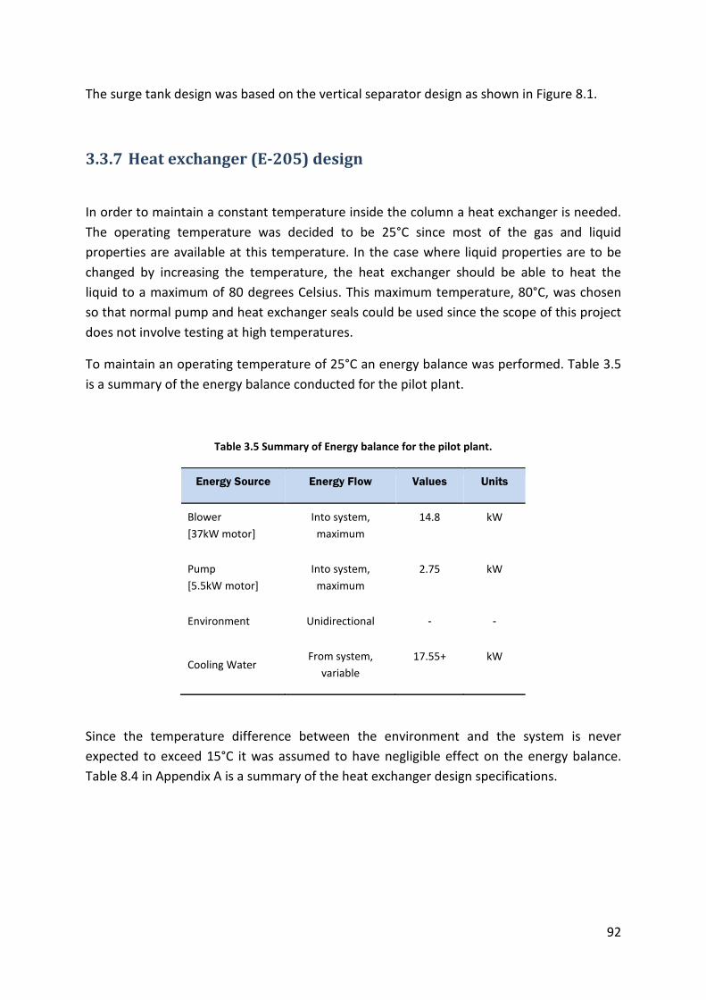
92

The surge tank design was based on the vertical separator design as shown in Figure 8.1.

3.3.7 Heat exchanger (E-205) design

In order to maintain a constant temperature inside the column a heat exchanger is needed.

The operating temperature was decided to be 25°C since most of the gas and liquid

properties are available at this temperature. In the case where liquid properties are to be

changed by increasing the temperature, the heat exchanger should be able to heat the

liquid to a maximum of 80 degrees Celsius. This maximum temperature, 80°C, was chosen

so that normal pump and heat exchanger seals could be used since the scope of this project

does not involve testing at high temperatures.

To maintain an operating temperature of 25°C an energy balance was performed. Table 3.5

is a summary of the energy balance conducted for the pilot plant.

Table 3.5 Summary of Energy balance for the pilot plant.

Energy Source Energy Flow Values Units

Blower

[37kW motor]

Into system,

maximum

14.8 kW

Pump

[5.5kW motor]

Into system,

maximum

2.75 kW

Environment Unidirectional - -

Cooling Water From system,

variable

17.55+ kW

Since the temperature difference between the environment and the system is never

expected to exceed 15°C it was assumed to have negligible effect on the energy balance.

Table 8.4 in Appendix A is a summary of the heat exchanger design specifications.

93

3.3.8 Venturi design (E-103)

It was impossible to find one gas flow meter that would accurately measure the gas flow for

all the different gasses mentioned in Table 3.2. The other options were therefore to use a

Pitot tube, Orifice plate or venturi. The latter was found to be more accurate with a friction

coefficient that is a more linear function of the Reynolds number over the operating range.

The challenge was then to design the venturi meter, construct it and to add the necessary

sensors that will be used to measure and record the gas mass flow. The detail venturi design

with correlations and measurements can be found in section 8.2.1 of Appendix A.

3.3.9 System pressure control

In the case where flammable liquids and gasses other than air will be used the system

pressure should be maintained slightly above atmospheric pressure. To achieve this a

pressure control valve (PCV-107, see Figure 3.8) is place between the regulator valve of the

gas cylinder and the surge tank (E-101). To prevent the system from overpressure a liquid

seal was constructed and attached to the surge tank. The liquid height in the seal (see

pipeline 39 in Figure 3.8) will prevent the system from exceeding a pressure of 10kPa above

the atmospheric pressure.

3.3.10 Sensor placing

Digital pressure transmitters:

By measuring the pressure drop across the different trays and sections in the column, the

system stability can be monitored. The pressure drop across the de-entrainment section

indicates if the mist-eliminator pad is flooded, accumulating liquid, and whether the liquid

hold-up on the de-entrainment tray stays constant during sampling. Digital differential

pressure transmitters were therefore placed:

1. Over the Chimney (gas distributing section) tray (DPE-201)

2. Over Test trays 1 and 2 (DPE-203/2)

3. Over the de-entrainment tray (DPE-204)

4. Over the mist eliminator pad (DPE-205)

5. Between the Venturi Pressure Tapings (DPE-101)

6. The bottom of the entrainment and weeping hold-up tanks (DPE-208/7)

94

Absolute pressure transmitters:

The absolute pressure transmitters are used to determine the gas physical properties

(density) at the venturi (PE-102) and test tray 1 (PE-206).

Temperature sensors:

In order to control and monitor the system thermal stability and temperature, sensors were

placed:

1. At the exit of the heat exchanger, to control temperature (TE-201)

2. At the inlet to the column (TE-202)

3. In the liquid flow path on test tray 1 (TE-203)

4. In the gas flow path between test tray 1 and 2 (TE-204)

5. In the liquid flow path on test tray 2 (TE-205)

6. In the gas flow path between test tray 2 and the chimney tray (TE-206)

7. In the liquid sump close to the exit (TE-207)

8. At the liquid flow meter to convert volumetric flow to mass flow when needed

(TE- 210)

9. In the weeping and entrainment hold-up vessels (TE-208/9)

10. At the gas inlet to the column (TE-102)

11. At the venturi input to compensate for temperature (TE-101)

Liquid flow meter:

It was decided to place the liquid flow meter just after the pump before the control valve

and bypass pipe line. Since the pump and liquid flow meter have to be shared between the

tray column and a packed column (for another project) and due to space restrictions, this

was the optimum place. In the case of control valve failure, the liquid flow rate through the

bypass line can also be measured.

Venturi flow meter:

It was decided to place the venturi between the gas outlet of the column and the surge

tank. Due to the limited space available, this was the best position. The venturi was

estimated to weigh approximately 73 kg. At the selected placing an overhead crane was able

to move and transport the venturi.

95

3.3.11 Sensor sizing and selection

Differential pressure transmitters:

From tray pressure drop calculations and suggestions made by Koch-Glitsch all the

differential pressure transmitters that were placed across the different column sections was

scaled to measure a range of 0 – 4kPa. This range could be converted by the PLC analog card

to give a 0 – 4000 digital range, meaning 1000 digital points per 1kPa pressure drop. The

same range was chosen for the weeping and entrainment hold-up tanks based on their

height of 0.4m.

According to Eq. 8.3 a pressure drop of 4kPa across the venturi would equal a superficial gas

(based on air) velocity of 7.9 m/s. Excessive entrainment was achieved at superficial

velocities of 5.5 m/s. All the differential pressure transmitters have a turndown ratio of 15:1.

It was therefore decided to purchase differential pressure transmitters that can measure a

maximum pressure drop of 10 kPa. Detail specifications of the transmitters used are shown

in Table 8.5.

Absolute pressure transmitters:

The absolute system pressure is close to atmospheric pressure. The transmitter which

would be able to measure this small range has a range of 0-200kPa (abs). To further increase

the accuracy and resolution of the measurement the sensors were scaled so that 80kPa

equals 4mA (the minimum value) and 120kPa equals 20mA (the maximum value). By

reducing the sensor output range the resolution of the measurement increases. Detail

specifications of the transmitters used are shown in Table 8.6.

Temperature sensors:

Since accuracy is preferred over measuring range and response time, it was decided to use

PT-100 (Platinum Resistance Thermometers) temperature probes instead of thermocouple

type sensors.

Liquid flow meter:

The only flow meter that can accurately measure the flow rate for the range of liquids

shown in Table 3.3, is a positive displacement flow meter. An oval gear type flow meter that

measures a flow rate from 1.8 - 27 m3/h was purchased and installed. Detail specifications

of the flow meter used are shown in Table 8.7.

96

Gas flow meter:

To verify the accuracy of the venturi meter for other gasses, a CO2 mass flow meter (FE-

102)1 was purchased and placed in the gas line. Detail specifications of the flow meter used

are shown in Table 8.8.

3.3.12 HAZOP, Safety interlocks and control philosophy

In order to develop the control philosophy and strategy a hazard and operability study

(HAZOP) was conducted in section 8.3 of Appendix A. Based on the HAZOP study a safety

interlock strategy was developed to reduce the probability of equipment (pump, blower,

heaters) failure when operating close to limiting design conditions.

The following are the control objectives:

1. Column temperature, by controlling the liquid temperature

2. Liquid flow rate

3. Gas flow rate

4. Sampling the entrainment and weeping rate.

5. Control hot water bath temperature

Table 8.11 is a summary of the control philosophy based on the HAZOP study and the

control objectives. The control philosophy was used as an aid to program the control

system.

3.3.13 Control system design

The control system can be divided between the control panel with the controllers and

switch gear, the human machine interface (HMI) that enable communication between the

user and the control panel, and the software with the automation and control loops.

1 See Figure 3.8

97

Control panel hardware:

The function of the control panel hardware is to;

1. Convert the analog signals form the different sensors to digital values without

losing accuracy. The analog to digital conversion cards has a 12bit resolution

meaning it can measure the 0 – 20mA range with a 5µA resolution.

2. Convert digital set points to analog signals for the different valve controllers and

actuators.

3. Use the digital values for comparative control.

4. Switch relays and contactors that activate motors and pneumatic valves.

5. Provide safety interlocking by monitoring device operating parameters.

6. Provide the pump and blower with motor rotational speed control through

frequency inverters

7. Power all the instruments and sensors

8. Control temperatures, flow rates and pressures

It was therefore decided to use Programmable Logic Controllers (PLCs) with temperature

controllers, analog to digital conversion cards, digital to analog conversion cards, and

frequency inverters to control the pilot plant operation.

The human machine interface (HMI):

The function of the human machine interface is to:

1. Link the operator with the control system

2. Provide the operator with visual information regarding the system parameters

3. Allow the operator to change set points and make the required selections.

It was therefore decided to use a touch panel as HMI. The touch panel can be used for data

logging and was found to be user friendly and inexpensive compared to computer systems.

Since the amount of data registers that had to be logged exceeded the number of columns

provided in the touch panel data tables, alternative methods were found and will be

discussed in section 3.3.14.

The software:

The software was programmed to:

1. Execute comparative control

2. Allocate data registers

3. Convert the digital values from the analog cards, using math and scaling, to flow

rates, temperatures, pressures, vibrations, motor load current, and valve

positions.

98

4. Create communication between the PLC, HMI, temperature controllers and

frequency inverters.

The PLC and HIM has their own unique software that was programmed to execute the

control and automation requirements.

3.3.14 Data recording

Special software was purchased to record the data. The software is computer based and

required communication between the computer and the PLC. The software will then

monitor the appointed data registers, every 300ms, and log the data every 2 seconds into a

.CSV file which can be accessed using Microsoft Excel.

3.3.15 Piping and instrumentation diagram

Based on the detail design requirements and control objectives the P&IDs were constructed

as shown in Figure 3.8 and Figure 3.9.

99

Figure 3.8 The Piping and Instrumentation Diagram of the experimental setup.

TE

203

DPI

203

TE

207

LI

201

E-201

V-206

V-207

DPI

204

DPI

202

DPI

205

TE

205

PI

206

TE

202

TE

204

TE

206

E-101

TE

201H

Liquid

Sampling/

Draining

Liquid Loading

Gas Loading

P

P

DPI

201

TIR

203

DPE

203

DPE

202

DPE

201

DPE

204

DPE

205

PE

206

TI

204

TI

208

TIR

202

TIR

207

To Packed

Column

From Packed

Column

DPI

101

DPE

101

TIR

206

TI

208

TIR

205

Settled liquid

Draining Point

TIR

201

PE

102

TE

101

TI

101

PIR

102

From Packed

Column

To Packed

Column

FIR

101

1

2

3

4

5

7

6

8

9

1013

14

15

17 18

19

20

21

23

24

22

29

To Heating/

Cooling Line

From Heating/

Cooling line

30

31

Gas Draining

32

32

33

34

35

37

38

39

PV-201

PV-202

MV-203

MV-204 MV-206PCV-205

MV-207

PV-208

MV-209 MV-210

PV-211

PV-212

PV-213

PV-214

PV-215 PV-216

RVCV-101

FY

101

H

L

TE

102

TIR

102

PCV-107

PY

102

FE

201

FIR

201

FC

201SC

201

H

L

IIR

201

H

L

DPE

207

FIR

207

H

L

DPE

208

H

L

LY

208

LY

207

TE

103

TIR

103

TE

104

TIR

104

FIR

208

SE

103

SIR

103

SE

104

SIR

104

H H H H

IIR

101

EY

101

E-205

E-204

E-102

TE

201C

PC

102

11

FIR

102

FE

102

MV-202 MV-203

E-103

V-103

36

Ventilation41

12

TIR

209TIR

208

TIR

210

To TIC 201

Chimney Tray

Test Tray 2

Test Tray 1

V-102

V-104

V-105

V-106

H

L

H

L

V-108

H

L

SC

105

16

46

100

Figure 3.9 The Piping and Instrumentation Diagram of the hot-and-cold water supply section.

Figure 3.10 Detailed drawing of some of the components of the experimental setup.

E-13

E-13

V-49

TE

301

TY

301

V-46

CW Feed

TIC

301

V-48

V-47

LE

301

LAL

301

LAH

301

LY

301

TT

301

To E-205

From E-205

CW

Return

23

24

25

26

27

28

V-45

43

44

45

From TIC 201

Hot Water

Bath

101

3.4 Experimental procedure

The experimental procedure will be explained chronologically from the start-up of the

experimental setup until sampling of the data. In order to follow the explanations please

refer to Figure 3.8.

Experimental start-up procedure:

1. Start the blower (E-102) with an inverter output frequency setting of around 28Hz.

As soon as the blower finishes the start-up cycle the radial vane control valve

(RVCV-101) is opened to 30%. At this setting small fluctuations in the valve

position will not affect the gas flow rate as much as when the valve position is

below 25%.

2. Enter a liquid flow rate set value (10 – 20m3/h) on the touch panel. Wait

approximately 30 seconds for the liquid flow rate control valve (PCV-205) to open,

and then start the liquid pump (E-204).

3. After the pump (E-204) has finished the start-up cycle, switch the three way ball

valve PV-212 so that the liquid flow through the column (line 9) and not the bypass

(line 8) leading to the sump.

4. Switch the cooling water system on and enter 24.8 °C as the liquid temperature

set point, which will ensure an average column temperature of approximately

25°C.

5. Monitor the liquid level in the de-entrainment section to prevent the de-

entrainment devices from flooding or malfunctioning (when liquid starts to exit

the gas-liquid separating devices in the de-entrainment section, flooding occurs).

The liquid level in the de-entrainment section should not exceed 70mm. If the de-

entrainment section flooded the blower rotational speed must be reduced by

reducing the inverter output frequency.

6. The liquid separated by the de-entrainment section exits through a pipeline (line

16), flush with the tray deck, through entrainment hold-up tank (MV-204) to either

the entrainment hold-up tank (MV-202) or the sump (line 15). For small entrained

liquid rates (L’ < 0.07 kg/s) MV-204 must be used to measure entrainment.

7. The liquid captured by the weeping collection (chimney) tray exits through a

pipeline (line 19), flush with the tray deck, to either the weeping hold-up tank

(MV-203) or the sump (line 18).

8. Before commencing with experiments the entrainment and weeping hold-up tanks

should be flushed with liquid (by simulating entrainment and weeping) to ensure

the vessel temperatures are simular to the column temperatures.

102

Experimental procedure:

1. Set the liquid flow rate. To ensure a constant liquid flow rate the control valve will

be fully opened by selecting a liquid flow rate set value of 20m3/h. The pump

rotational speed should then be increased or decreased, by changing the inverter

output frequency (15 - 50Hz), until the liquid flow rate is approximately 0.5 m3/h

above the required flow rate. Enter the required liquid flow rate set point so that

the control valve (PCV-205) can control the liquid flow rate continuously.

2. Change the gas flow rate (by changing the blower rotational speed) until there is a

10 and 70mm visible liquid level in the de-entrainment section.

3. 5 minutes after the column temperature, the differential pressure of each section,

gas flow rate, and liquid flow rate has stabilized a sample should be taken. To

determine if the system is stable temperature, pressure, and gas and liquid flow

rate graphs are plotted on the HMI. Approximately 5 minutes after all the graphs

show zero change (gradient of zero) the system is defined as stable.

a. Automated sequence for small liquid entrainment rates (L’ < 0.07 kg/s):

i. The liquid exiting the de-entrainment section will fill MV-204 by

closing PV-217.

ii. The mass of the liquid inside the tank (MV-204) is logged against

time until the sample volume is reached whereafter PV-217 will

open to drain the liquid to the sump.

b. Automated sequence for larger liquid entrainment rates (L’ > 0.07 kg/s):

i. The liquid exiting the de-entrainment section will fill the hold-up

tank (MV-202) by switching PV-213. The mass of the liquid in the

tank is logged against time. As soon as the sample volume (which is

pre-selected) is reached PV-213 will switch back so that the de-

entrained liquid can flow to the sump.

ii. PV-215 will then open followed by PV-201 so that the pump can

empty the tank. Just before the liquid level in the tank reaches the

bottom (5-7 litres remaining) PV-215 and PV-201 will switch back so

that the pump is fed from the column sump.

4. This procedure should be repeated 3-4 times for each liquid and gas flow rate

setting to ensure accurate results and to determine if the system was stable.

Change the gas flow rate (increase or decrease in random order) to measure a

different entrainment rate. Four to five gas flow rates should be used to measure

the entrainment rate per liquid flow rate.

5. Change the liquid flow rate (increased or decreased in random order) and follow

the same procedure as described in steps 1 – 6.

6. To test the system repeatability experimental conditions (flow rates) should be

repeated on different dates and compared as shown in Figure 8.5.

103

7. For liquid flow rates below 7m3/h (40m

3/(h.m)) the downcomer escape area

should reduced to prevent gas from bypassing through the downcomer (due to an

insufficient down comer seal which will occur at liquid velocities below 2.3 m/s). A

sensitivity analysis, see Figure 4.1 to Figure 4.3, was conducted to test the

influence of the change in downcomer escape area on entrainment for certain

liquid rates.

3.5 Factors affecting measurement accuracy

To ensure that the measurements are accurate, all the sensors were calibrated and their

measurements verified. A detail summary of the calibration and verification procedures is

given in section 8.4 of Appendix A which involved:

1. Calibration of the control system.

2. Calibrating the entrainment and weeping hold-up tanks (MV-202/3/4).

3. Testing for gas and liquid leakages.

4. Verification of sensor measurements.

5. Testing the system with air and water.

6. Verification of system repeatability.

All the sensors purchased were calibrated prior to delivery and their calibration certificates

can be found in the in the attached CD at the back of the thesis (or on special request to the

author).

To ensure each sample is representative of the amount of entrainment in the system the

following is of utmost importance when tanking a sample:

1. The pressure drop across each tray should be stable (zero gradient on HMI graph).

The pressure drop represents the liquid hold-up on the tray which affects the

amount of entrainment.

2. The gas and liquid flow rates should be stable since they both directly affect

entrainment.

3. Gas and liquid temperatures and pressure should be stable since these operating

conditions will determine the gas and liquid physical properties which in turn will

affect the amount of entrainment.

104

3.6 Data processing

The raw data was processed using MATLAB and the graphs fitted in Excel. A detailed

description of the data processing methods can be found in Appendix A, section 8.6.

105

4 Experimental results & discussion

Tests were conducted with an air/water system. The results will be presented and compared

with entrainment predictive trends from the literature. Since most of the correlations in the

literature define entrainment as the mass of liquid entrained over the mass of rising gas, a

conversion was made to compare the entrainment as mass of liquid entrained over mass of

liquid entering the tray. Only some of the authors reviewed in the literature review section

(section 2.1) published entrainment prediction correlations as shown in Table 2.17. In this

work equations 2.2, 2.12, 2.38, 2.41, 2.43, 2.57 and 2.58 were used to compare the

experimental data with the published entrainment trends. Final conclusions will be made in

chapter 5.

4.1 Gas and liquid flow rates

Kister and Haas (1988) and Bennett et al. (1995) proposed entrainment prediction

correlations (from various data sources) for a liquid flow rate range of 4 – 130 m3/(h.m). It

was therefore decided to test between 17.2 – 112.9 m3/(h.m) which was the capacity range

for the experimental setup. Most of the authors tested for a gas superficial velocity range of

0.9 – 3.7 m/s. Since one of the aims of this investigation is to investigate excessive

entrainment it was decided to test for a gas superficial velocity range of 3.4 – 4.6 m/s. This

velocity range resulted in a 5 – 20% entrainment range. The overlapping of gas velocity test

ranges with the application ranges of the entrainment prediction curves will also show what

happens when these entrainment prediction correlations are extrapolated beyond their

respective ranges. Table 4.1 is a summary of the gas and liquid flow rates that were used

during testing:

Table 4.1 Gas and liquid flow rate ranges used during testing.

Minimum Maximum

QL

[m3/(h.m)]

17.2 112.9

us [m/s] 3.4 4.6

106

4.2 Experimental results

Since the liquid velocity increases as the downcomer escape area decreases for a constant

volumetric flow rate, the momentum of the liquid increases which might influence the

entrainment rate (Zuiderweg 1982 based hydrodynamic characterisation on liquid velocity).

The first step was therefore to test if the escape area under the downcomer, therefore the

liquid velocity, has an influence on the percentage entrainment. It was also necessary to

characterise the point where gas start to bypass through the downcomer. Gas that bypasses

through the downcomer will have a negative effect on entrainment since only some of the

measured gas will pass through the liquid on the tray. The influence of gas velocity on

entrainment for a given liquid flow rate was then recorded to characterise and correlate

(Figure 8.6 and Figure 8.7) the dependency of entrainment on gas velocity. The final step

was to compare the generated entrainment results with the entrainment prediction

correlations proposed by the authors mentioned in Table 2.17.

4.2.1 Sensitivity analysis of the downcomer escape area on

entrainment

In order to determine the point where gas bypass through the downcomer starts, three

different downcomer escape areas were used for the lower (28.6 and 40 m3/(h.m)) liquid

flow rates and two downcomer escape areas for the higher liquid flow rates. It was

observed visually, and confirmed experimentally in Figure 4.1, that at liquid flow rates of 30

m3/(h.m) and smaller there was not sufficient downcomer backup (liquid level in the

downcomer too low) to seal the downcomer escape area for the largest setting (Aesc =

8.575×10-3

m2). The gas therefore bypassed through the downcomer and the measured

amount of entrainment was less than for the other two smaller downcomer area of escape

settings. This was confirmed in the results as shown in Figure 4.1 , below. There was

however no difference in the measured entrainment rates between the smaller two

downcomer escape area settings for the low liquid flow rate of 28.6 m3/(h.m).

At a higher liquid flow rate of 40 m3/(h.m) the downcomer escape area, perfectly sealed,

had no effect on the measured entrainment as shown in Figure 4.2 below. Therefore the

only effect the downcomer escape area has on entrainment is when the escape area is large

enough for gas to bypass through the downcomer due to insufficient liquid backup in the

downcomer. It was decided to use the liquid velocity as a guideline to ensure operation with

a positive downcomer seal. Table 4.2 was constructed to assist in determining the liquid

flow rates for each downcomer area of escape setting. From Table 4.2 it is clear that the

liquid velocity through the downcomer escape area should be above 0.23m/s to ensure a

sufficient downcomer seal. This corresponded with the liquid velocity range of 0.3 – 0.6m/s

107

proposed by Koch-Glitsch the tray manufacturer. Therefore, if the liquid velocity is too high

the liquid level in the downcomer will be too high causing the downcomer to flood, whereas

a low liquid velocity will result in gas bypass through the downcomer.

Figure 4.1 The influence of the downcomer escape area on entrainment as a function of the capacity factor

( )/p p g L gC u ρ ρ ρ= − for a liquid flow rate of 28.6 m3/(h.m).

0%

10%

20%

30%

40%

50%

60%

0.12 0.13 0.14 0.15 0.16 0.17

L'/L

Cp [m/s]

Aesc = 3.33E-3 m2,

QL = 28.6 m3/(h.m)

Aesc = 5.4E-3 m2, QL

= 28.6 m3/(h.m)

Aesc = 8.575E-3 m2,

QL = 28.6 m3/(h.m)

108


( )/p p g L gC u ρ ρ ρ= − for a liquid flow rate of 40 m3/(h.m).

To test the hypothesis that the downcomer escape area does not have any influence on

entrainment, another comparison was made between two downcomer escape area settings

for a liquid flow rate of 57.2m3/(h.m), as shown in Figure 4.3.

0%

5%

10%

15%

20%

25%

30%

0.13 0.14 0.15 0.16

L'/L

Cp [m/s]

Aesc = 3.33E-3 m2,

QL = 40 m3/(h.m)

Aesc = 5.4E-3 m2,

QL = 40 m3/(h.m)

Aesc = 8.575E-3 m2,

QL = 40 m3/(h.m)

109


( )/p p g L gC u ρ ρ ρ= − for a liquid flow rate of 57.2 m3/(h.m).

Table 4.2 Liquid velocity for each liquid flow rate against the downcomer escape area

QL

[m3/(h.m)]

uL [m/s] for

Aesc of

3.33×10-3 m2

uL [m/s] for

Aesc of

5.4×10-3 m2

uL [m/s] for

Aesc of

8.575×10-3 m2

28.6 0.41 0.26 0.16

40 0.58 0.36 0.23

57.2 - 0.51 0.32

112.9 - - 0.64

0%

5%

10%

15%

20%

25%

30%

0.13 0.14 0.15 0.16 0.17

L'/L

Cp [m/s]

Aesc = 5.4E-3 m2,

QL = 57.2 m3/(h.m)

Aesc = 8.575E-3 m2,

QL = 57.2 m3/(h.m)

Gas Bypass

110

4.2.2 Entrainment data

In order to generate entrainment data for the air/water system, with physical properties as

shown in Table 4.3, it was decided to systematically vary the gas velocity for each liquid flow

rate setting. The reason for this was that it is easier to control the liquid flow rate than the

gas flow rate. At low liquid flow rates the downcomer escape area had to be changed

discarding the option of maintaining a constant gas flow rate and changing the liquid flow

rate.

The liquid flow rate was systematically chosen depending on the downcomer area of escape

setting and the criteria given in Table 4.2. The gas flow rate was then changed until a liquid

level was visible on the de-entrainment tray. Three to four entrainment measurements

were taken at each gas/liquid flow rate setting after which the gas velocity was either

increased or decreased. The three to four measurements were used directly to generate the

entrainment trends and none of the data points were averaged. The raw data can be found

in Appendix A, section 8.5. Figure 4.4 and Figure 4.5 shows that by increasing the capacity

factor, Cp, and hence the gas velocity for a given liquid rate, an increase in entrainment

results. The rate at which the gas velocity increases entrainment differs between the liquid

flow rates.

Table 4.3 Air/Water system physical properties used during experimental runs.

ρL

[kg/m3]

ρG

[kg/m3]

σ

[mN.s]

µ

[mPa.s]

1020 - 1040 1.16 - 1.19 66 - 68 0.8 – 0.9

111

Figure 4.4 The influence of the capacity factor (gas velocity) on entrainment for individual liquid flow rate

settings from 17.2 – 74.2 m3/(h.m).

Figure 4.4 shows that as the liquid flow rate increases from 17.2 – 74.2 m3/(h.m), the gas

velocity has to be increased to maintain a certain percentage entrainment. As the liquid flow

rate is increased from 79.9 – 112.9 m3/(h.m), Figure 4.5, the gas velocity has to be reduced

to maintain the percentage entrainment.

0%

5%

10%

15%

20%

25%

30%

35%

40%

45%

50%

0.12 0.13 0.14 0.15 0.16 0.17

L'/L

Cp [m/s]

QL = 17.2 m3/(h.m)

QL = 28.6 m3/(h.m)

QL = 40 m3/(h.m)

QL = 57.2 m3/(h.m)

QL = 74.2 m3/(h.m)

Increasing Liquid Flow Rate

112

Figure 4.5 The influence of the capacity factor (gas velocity) on entrainment for individual liquid flow rate

settings from 79.9 –112.9 m3/(h.m).

In order to show the effect of the capacity factor and liquid flow rate on the entrainment

rate, Figure 4.6 was constructed. This was achieved by manipulating the capacity factor so

that a constant entrainment rate was achieved. Figure 4.6 shows that for a liquid range from

17.2 – 74.2 m3/(h.m) the gas velocity (capacity factor) had to be increased to maintain the

percentage entrainment. As the liquid flow rate is increased from 79.9 – 112.9 m3/(h.m) the

gas velocity had to be reduced to maintain the percentage entrainment. There are two main

possible reasons for this behaviour. The first possibility is explained by Kister and Haas

(1981, 1988) as a change between the flow regimes. They suggest that in the spray regime

the gas velocity has to increase with increasing liquid flow rate, since the momentum effects

of the cross flowing liquid will suppress jetting at the sieve tray holes and therefore reduce

entrainment. As the liquid flow rate increase the liquid hold-up increases to the point where

the froth layer is much closer to the tray above, which is commonly found in the froth

regime. The droplets ejecting from the froth layer in the froth regime will then have a

shorter distance to travel in order to reach the tray above. Consequently, entrainment is

favoured by the larger liquid hold-up and the gas velocity has to be reduced to reduce the

ejection velocity of the liquid droplets projecting from the froth layer. Colwell (1981) also

showed that by reducing the gas velocity the froth height will be reduced resulting in less

entrainment.

0%

5%

10%

15%

20%

25%

0.13 0.14 0.15 0.16 0.17

L'/L

Cp [m/s]

QL = 74.2 m3/(h.m)

QL = 79.9 m3/(h.m)

QL = 96.8 m3/(h.m)

QL = 112.9 m3/(h.m)

Increasing Liquid Flow

Rate

113

Figure 4.7 shows that, when entrainment is measured as L’/G, the result is a more complex

trend with a possible change in flow regime at low liquid (<30m3/(h.m)) flow rates. A more

simple comparison between the two different methods for measuring entrainment and the

influence of the liquid flow rate was done in Figure 2.10.

Figure 4.6 Influence of gas and liquid rates on entrainment where entrainment is measured as mass liquid

entrained per mass of liquid entering the tray.

0.11

0.12

0.13

0.14

0.15

0.16

0.17

0 20 40 60 80 100 120

Cp

[m/s

]

QL [m3/(h.m)]

L'/L = 5%

L'/L = 10%

L'/L = 20%

114

Figure 4.7 Influence of gas and liquid rates on entrainment where entrainment is measured as mass liquid

entrained per mass of rising vapour.

The second reason for the change in gas velocity for a given percentage entrainment follows

on the increasing liquid hold-up theory proposed by Kister et al. (1981) and Kister and Haas

(1988). As the liquid flow rate is increased the time or distance required for the froth to

develop changes due to the increased horizontal momentum of the cross flowing liquid. As

the liquid flow rate increases the momentum of the horizontal flowing liquid increases.

Therefore in order to develop a uniform froth a longer flow path is needed at higher liquid

flow rates. Since the liquid flow path length of the column used in this work was constant at

only 455mm the froth is not fully developed for liquid flow rates higher than 74.2 m3/(h.m).

This observation was also made visually when it was noticed that the froth was pushed up

against the opposite wall of the column above the downcomer, see Figure 4.8.

0.11

0.12

0.13

0.14

0.15

0.16

0.17

0 20 40 60 80 100 120

Cp

[m/s

]

QL [m3/(h.m)]

L'/G = 40%

L'/G = 80%

L'/G = 120%

115

Figure 4.8 (a) Uniform developed froth. (b) Non-uniform developed froth.

As the froth layer pushed up against the column wall the froth layer happens to be much

closer to the tray above. This caused most of the droplets ejecting from the froth layer to

reach the tray above and increase the percentage entrainment and the gas velocity (Cp) had

to be reduced to maintain constant entrainment. According to the flow regime criteria

proposed by Kister and Haas (1988) (the largest value between Eq. 2.38, 2.41 and 2.43 ), and

Bennett et al. (1995) (Eq. 2.63), the operating regime proposed by this work is the froth

regime and never changes. The reason for the increasing entrainment is therefore caused by

the increasing liquid flow rate which resulted in the formation of a non-uniform froth layer

positioned closer to the tray above. No correlation regarding froth development as a

function of the flow path length was found during the literature survey. Hunt et al. (1955)

mentioned that they chose to use no liquid cross flow in their 152mm round column due to

“the unreliability of the performance of liquid overflow weirs in a 152mm diameter

column”. It was impossible to correlate the effect of flow path length and liquid flow rate

on entrainment since this requires the construction of various columns with similar tray

geometry.

Kister and Haas (1988) and others suggests that the amount of liquid entrained per mass of

gas flowing will increase as the liquid flow rate is increased past the regime transition. This

was found to be true as will be shown in Figure 4.9. When the different ways of measuring

entrainment are compared (see Figure 4.9) it can be seen that while the entrainment over

gas relationship increases the entrainment per liquid load stayed constant. This confirms the

findings by Kister and Haas (1988) that an increase in liquid flow rate will increase

entrainment (L’/G) in the froth regime, however, if entrainment is related to the amount of

liquid on the tray the gas velocity has to be increased to maintain a constant entrainment

(L’/L) rate as shown in Figure 4.10. Figure 4.10 was constructed from 5% experimental

Uniform Froth Layer

Uniform Froth Layer

Non-uniform Froth Layer

Non-uniform Froth Layer

(a) (b)

Tray

Column

Wall

116

entrainment (L’/L) data. To show the difference between the two methods of measuring

entrainment the same 5% (L’/L) data is presented as mass liquid entrained per mass rising

gas (L’/G) in Figure 4.9.

Figure 4.9 Comparing the different methods of measuring the entrainment rate.

Therefore, an increase in entrainment (L’/G) does not necessarily mean that the fraction of

liquid on the tray that is entrained (L’/L) increased as well. This method is just another

perspective on the influence of liquid flow rate on entrainment.

4.3 Comparing results with predictive trends

The generated results are compared with the entrainment predictive trends (see Table 2.17)

in Figure 4.10 for the conditions used in this work (see Table 4.1 and Table 3.4).

By using the flow regime criteria developed by Kister and Haas (1988) and Bennet et al.

(1995) is was established that the operating regime is the froth regime for liquid flow rates

above 40 m3/(h.m). For liquid flow rates below 40 m

3/(h.m) Kister and Haas (1988) suggests

spray regime conditions while Bennett et al. (1995) suggests a froth regime. Hunt et al.

y = 0.0053x

y = 0.1066x

2

4

6

8

10

12

14

16

0%

10%

20%

30%

40%

50%

60%

70%

0 20 40 60 80 100 120

L/G

Ra

tio

En

tra

inm

en

t [L

'/L]

QL [m3/(h.m)]

L'/L = 5%

L'/G

L/G

117

(1955) and Thomas and Ogboja (1978) did not develop any regime defining correlations. The

correlation by Thomas and Ogboja (1978) failed under the conditions required to obtain 5%

L’/L entrainment and 40% L’/G entrainment since they measured much lower entrainment

rates. Their correlation could therefore not be compared with the experimental data. In

Figure 4.10 the 5% entrainment predictive curves are plotted as a function of the capacity

factor (based on the gas velocity) and liquid flow rate and compared with the

experimentally generated results.

Figure 4.10 Comparing entrainment predictive trends with experimentally generated entrainment data with

entrainment measured as L’/L.

To show how the correlations compared with the experimental data when entrainment is

measured as L’/G Figure 4.11 was constructed. The sudden inflexion in the correlation by

Kister and Haas (1988) in both Figure 4.10 and Figure 4.11 at low liquid rates is due to their

anticipation of a change in flow regime from spray to froth regime. It is expected that the

correlation of Kister and Haas (1988) would follow the correlation developed by Hunt et al.

(1955) since Kister and Haas based their froth regime correlation on that of Hunt et al. with

an empirical hole diameter dependence and a correction term for non-uniformity of the

froth at low clear liquid heights.

0.00

0.05

0.10

0.15

0.20

0.25

0.30

0 20 40 60 80 100 120

Cp

[m/s

]

QL [m3/(h.m)]

Exp (2009) L'/L

= 5%

Hunt et. al

(1955)

L'/L=5%

K & H (1988)

L'/L = 5%

Bennett et. al

(1995) L'/L

= 5%

118

Figure 4.11 Comparing entrainment predictive trends with experimentally generated entrainment data

where entrainment is measured as L’/G.

Figure 4.10 shows that the shape of the generated entrainment trends between Hunt et al.

(1955), Bennett et al. (1995), and the experimental data from this work have a similar

curvature. The prediction made by the correlation from Kister and Haas (1988) does not

follow the same trend as the propositions made by the other authors and the generated

data. The differences between the generated data and each one of the predictive trends will

be discussed in detail below starting with Hunt et al. (1955) and ending with the

experimental data.

Since no clear height data was generated in this work, the correlation by Colwell (1981) (Eq.

2.23) was used to calculate the clear liquid heights which were needed for the entrainment

prediction correlation developed by Hunt et al. (1955). Kister and Haas (1988) also used

Colwell’s correlation to determine froth heights for entrainment data sets lacking froth

height and clear liquid height data. Hunt et al. (1955) assumed a constant froth density

throughout their gas and liquid flow rate range. Colwell (1981) showed that the froth

density is a function of the gas velocity, gas and liquid densities, fractional hole area and

clear liquid height. The assumption by Hunt et al. (1955) that a uniform froth density exists

is therefore an oversimplification. Hunt et al. (1955) tested with no liquid cross flow but

their correlation is a function of the clear liquid height which is a function of the liquid flow

0.00

0.05

0.10

0.15

0.20

0.25

0.30

0.35

0 20 40 60 80 100 120

Cp

[m/s

]

QL [m3/(h.m)]

Exp (2009) L'/G =

40%

Hunt et. al (1955)

L'/G=40%

K & H (1988) L'/G

= 40%

Bennett et. al

(1995) L'/G = 40%

119

rate. At high liquid rates the liquid hold-up will increase so that the froth layer is closer to

the tray above. Ejecting droplets therefore reaches the tray above much easier and gas

velocity has to be reduced. They therefore predicted higher gas velocities which can only

apply to no liquid cross-flow applications with lower liquid hold-up than applications with

liquid cross flow.

Kister and Haas (1988) used data from various sources in order to pursue a better

understanding of the influences of gas and liquid flow rates, and column and tray geometry

on entrainment. Even though they specified that their correlation can be used for large

range of liquid flow rates (2 – 130 m3/(h.m)) they do not have data which compares directly

to the geometrical parameters and gas and liquid flow rates presented in this work. The high

liquid flow rate (49 – 134 m3/(h.m)) data used to develop their correlation were obtained

from Lemieux and Scotti (1969) (presenting 5 trends in their work with only 24 data points

which included 3 different tray geometries) who used large hole diameter (12.7 – 25.4 mm)

trays with intermediate tray spacing (457 mm), low fractional hole area (0.069 – 0.094), low

weir height (25.4 mm) and intermediate gas velocities (Fs = 1.7 – 2.2 (kg/m)1/2

/s). Most of

the data used by Kister and Haas were developed with data obtained from low to

intermediate liquid flow rates (4 - 30 m3/(h.m)) and low to intermediate superficial gas

velocities (0.37 – 3 m/s). It is therefore understandable that even though the test ranges of

this work falls within most of the application ranges proposed by Kister and Haas (1988),

their correlation is extrapolated beyond an accurate range of application and deviations

from the experimental data generated in this work is expected.

The gas velocity range (3.3 – 4.0 m/s) used in this work, for the 5% entrainment curve, is

much higher than the application range (0.45 – 2.31 m/s) proposed for the correlation

developed by Bennett et al. (1995). It is, however, surprising how well their correlation

follows the data even though it is extrapolated beyond their proposed range of application.

The only significant deviation between the predictive correlation developed by Bennett et

al. and the experimental data were found at the 20% entrainment trends, shown in Figure

4.12. According to the correlation proposed by Bennett et al. a gas superficial velocity range

of 3.9 – 5.0 m/s is required to maintain 20% entrainment throughout the liquid range. This is

much higher than the velocity range, 3.9 – 4.5, covered during the experimental runs.

120

Figure 4.12 Comparison between the experimental data and that of Bennett et al. (1995) for 5 and 20%

entrainment.

The model developed by Bennett et al. (1995) assumed that for small, superficial gas

velocities (0.45 − 2.31 m/s), small Weber numbers (0.015 − 1.81) and a relatively large range

of Froude numbers (0.134 − 9.29) the effect of droplet drag can be neglected. Droplet drag

should only be considered at high superficial gas velocities and high Weber numbers. For

the 20% entrainment conditions in Figure 4.12 the superficial gas velocity (3.9 – 4.5 m/s),

Weber numbers (1.0 – 2.9) and Froude numbers (6.9 – 12.4) are much higher than the

ranges on which Bennett et al. (1995) based their correlations. For these high superficial gas

velocities the liquid droplet will be carried higher into the space above the froth than when

the effect of drag is neglected, resulting in more entrainment than predicted. The

correlation developed by Bennett et al. (1995) therefore under-predicts entrainment in high

superficial gas velocities and the error increases with increasing gas velocity as shown in

Figure 4.12.

0.10

0.11

0.12

0.13

0.14

0.15

0.16

0.17

0.18

0.19

0 20 40 60 80

Cp

[m/s

]

QL [m3/(h.m)]

Exp (2009) L'/L =

5%

Exp (2009) L'/L =

20%

Bennett et al.

(1995) L'/L = 5%

Bennet et. al (1995)

L'/L = 20%

121

4.3.1 Deviation between experimental data and predictive trend by

Bennett et al. (1995)

The deviation between the experimental data and the trend predicted by Bennett et al.

(1995) increases as the liquid flow rate exceeds 60 m3/(h.m). This is due to the undeveloped

froth (see Figure 4.8) which occurred during the experimental runs for large liquid flow

rates. Colwell (1981) showed that the froth height will increases with increasing gas velocity.

By increasing the gas velocity the velocity of the droplets ejecting from the froth layer is also

higher and more droplets will therefore reach the tray above. At liquid flow rates below 60

m3/(h.m) and for gas velocities above 3.5 m/s the correlation by Bennett et al. (1995) under-

predicts entrainment as previously discussed.

4.3.2 Comparison between experimental data and predictive trend by

Bennett et al. (1995) for a non-air/water (NAW) system

Bennett et al. (1995) acknowledges that their non-air/water entrainment prediction

correlation, Eq. 2.64, was developed from limited non-air/water data. Since the aim of

future work is to investigate the influence of gas and liquid physical properties in

entrainment, it was decided to test their prediction correlation for a non-air/water system

against the air/water entrainment data generated in this work.

Figure 4.13 shows that there is a significant difference between the entrainment prediction

trends developed by Bennett et al. for the air/water and non-air/water systems. It is clear

that more work is required to investigate the influence of gas and liquid physical properties

on entrainment in order to predict entrainment for non-air/water systems with higher

accuracy. Bennet et al. (1995) suggested that more non-air/water entrainment, froth height

and froth density data is required to develop an accurate entrainment prediction

correlation.

122

Figure 4.13 Comparison between the experimental data and that of Bennett et al. (1995) for 5% non-

air/water (NAW) and air/water (AW) entrainment prediction.

0.00

0.02

0.04

0.06

0.08

0.10

0.12

0.14

0.16

0.18

0 20 40 60 80 100 120

Cp

[m/s

]

QL [m3/(h.m)]

Exp (2009) L'/L = 5%

Bennett et. al (1995)

NAW L'/L = 5%

Bennett et. al (1995)

AW L'/L = 5%

123

5 Conclusions

One of the objectives of this study was to conduct a literature survey to gain insight into the

hydrodynamic behaviour inside sieve tray columns that constitutes entrainment. The

following conclusions are made based on the findings in the literature:

1. Tray and column geometry, gas and liquid flow rates, and gas and liquid physical

properties all have a significant influence on entrainment in both the froth and spray

regimes.

2. Most of the work done in the literature is based on air/water system data, which

does not account for the influence of gas and liquid physical properties found in

commercial distillation, absorption and stripping applications.

3. Bennett et al. (1995) proposed an entrainment prediction correlation for non-

air/water systems based on very little data. They acknowledge that the database is

limited and more entrainment, froth height and froth density data is required for

non-air/water systems to improve their correlation.

4. The entrainment prediction correlations developed by Kister and Haas (1988) and

Bennett et al. (1995) are based on data obtained from various sources with different

tray and column geometries and different sampling methods. In order to understand

the influence of gas and liquid physical properties and to eliminate the effect of

different tray and column geometries, a single column has to be used for all testing.

5. Van Sinderen et al. (2003) showed that entrainment is related to the amount of

liquid hold-up by using a constant liquid rate and varying weir heights. Kister and

Haas (1988) showed that an increase in liquid flow rate will also increase the liquid

hold-up. The question is therefore, what is the true influence of liquid flow rate on

entrainment other than changing the liquid hold-up and how does the horizontal

momentum of the flowing liquid influence the froth behaviour?

6. In the literature entrainment is measured as the mass of liquid entrained over the

mass of rising vapour. This measurement does not account for the amount of liquid

on the tray and it was decided to measure entrainment as the mass of liquid

entrained over the mass of liquid entering the tray. This measurement relates the

percentage entrainment to the liquid inventory on the tray and can therefore be

used to directly link entrainment with the mass transfer separation efficiency.

7. Most of the entrainment and hydrodynamic data mentioned and used in the

literature were generated between 1955 and 1981. There is therefore a need to test

new technology trays and to test the methods of old.

Based on the shortcomings found in the literature an experimental setup was designed,

constructed and commissioned which can:

1. Measure entrainment with high repeatability for a range of:

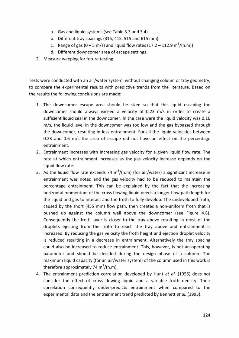
124

a. Gas and liquid systems (see Table 3.3 and 3.4)

b. Different tray spacings (315, 415, 515 and 615 mm)

c. Range of gas (0 – 5 m/s) and liquid flow rates (17.2 – 112.9 m3/(h.m))

d. Different downcomer area of escape settings

2. Measure weeping for future testing.

Tests were conducted with an air/water system, without changing column or tray geometry,

to compare the experimental results with predictive trends from the literature. Based on

the results the following conclusions are made:

1. The downcomer escape area should be sized so that the liquid escaping the

downcomer should always exceed a velocity of 0.23 m/s in order to create a

sufficient liquid seal in the downcomer. In the case were the liquid velocity was 0.16

m/s, the liquid level in the downcomer was too low and the gas bypassed through

the downcomer, resulting in less entrainment. For all the liquid velocities between

0.23 and 0.6 m/s the area of escape did not have an effect on the percentage

entrainment.

2. Entrainment increases with increasing gas velocity for a given liquid flow rate. The

rate at which entrainment increases as the gas velocity increase depends on the

liquid flow rate.

3. As the liquid flow rate exceeds 74 m3/(h.m) (for air/water) a significant increase in

entrainment was noted and the gas velocity had to be reduced to maintain the

percentage entrainment. This can be explained by the fact that the increasing

horizontal momentum of the cross flowing liquid needs a longer flow path length for

the liquid and gas to interact and the froth to fully develop. The undeveloped froth,

caused by the short (455 mm) flow path, then creates a non-uniform froth that is

pushed up against the column wall above the downcomer (see Figure 4.8).

Consequently the froth layer is closer to the tray above resulting in most of the

droplets ejecting from the froth to reach the tray above and entrainment is

increased. By reducing the gas velocity the froth height and ejection droplet velocity

is reduced resulting in a decrease in entrainment. Alternatively the tray spacing

could also be increased to reduce entrainment. This, however, is not an operating

parameter and should be decided during the design phase of a column. The

maximum liquid capacity (for an air/water system) of the column used in this work is

therefore approximately 74 m3/(h.m).

4. The entrainment prediction correlation developed by Hunt et al. (1955) does not

consider the effect of cross flowing liquid and a variable froth density. Their

correlation consequently under-predicts entrainment when compared to the

experimental data and the entrainment trend predicted by Bennett et al. (1995).

125

5. Thomas and Ogboja (1978) tested for lower tray spacings, lower liquid flow rates,

and smaller fractional hole area trays than presented in this work. The sampling

methods used by Thomas and Ogboja (1978) were questioned in section 2.4 of this

thesis under the critical evaluation section. Their correlation consequently under

predicts entrainment when compared the entrainment predictive trends of Hunt et

al. (1955), Kister and Haas (1988) and Bennett et al. (1995) (see Figure 2.9 to Figure

2.11).

6. Although the proposed application range of the correlation developed by Kister and

Haas (1988) overlaps the test range of this work it was found that their correlation

was extrapolated beyond an accurate range of application. Their correlation

followed a different trend than the predictive trends proposed by other authors and

the experimental data and under predicted entrainment.

7. Bennett et al. (1995) specified that the application range of their entrainment

prediction correlation is limited to a gas superficial velocity range of 0.45 – 2.31 m/s.

The superficial velocity range covered in the 5% experimental entrainment tests

ranged from 3.3 – 4.0 m/s. Even though their correlation was used at elevated gas

velocities, the entrainment prediction trend followed the results obtained during the

experimental runs very well. It was however noted that as the gas velocity is

increased further to 4.5 m/s the deviation between the experimental runs and their

prediction increased. They acknowledged that at high gas velocities and low surface

tension liquids a loss in accuracy is expected due to the fact that they don’t account

for the effects of droplet drag on entrainment. Their correlation therefore under

predicts entrainment at high gas velocities.

8. The non-air/water entrainment prediction correlation developed by Bennett et al.

(1995) was also tested against the experimentally obtained air/water results and a

significant difference was noted. More work is required to understand why there is

such a large difference but, Bennett et al. (1995) acknowledged that deviations are

expected due to the limited non-air/water data that was available during the

development of their correlation. They recommend that more entrainment, froth

height and froth density data is required.

126

6 Recommendations for future work

Based on the findings discussed in the conclusions, the following recommendations are

made:

1. Further testing is required to relate froth development with the flow path length. In

order to achieve this the flow path length should be increased while maintaining

constant tray fractional hole area, tray hole diameter, weir height and tray spacing.

By modelling entrainment data for three to four different column flow path lengths,

a better understanding of the influence of flow path length on froth development

will be achieved. The influence of flow path length is of great importance in multi-

pass trays where the flow path length available for froth development is much

shorter than on a single pass tray.

2. Large deviations were found with the non-air/water entrainment correlation

proposed by Bennett et al. (1995) and they acknowledged that more non-air/water

entrainment, froth height and froth density data is required to develop a more

accurate correlation. Further testing should therefore be conducted using systems

other than air/water to fully understand the influence of gas and liquid physical

properties on entrainment.

3. Using non-air/water, together with air/water entrainment data, the influence of gas

and liquid physical properties on entrainment should be correlated by modelling the

influence of gas and liquid density, liquid viscosity, and liquid surface tension on

entrainment. In order to develop a ‘physical property model’ dimensionless grouping

(most probably a combination of dimensionless groupings) of the physical properties

will be required.

4. The entrainment prediction correlations developed by Kister and Haas (1988) and

Bennett et al. (1995) are based on limited gas velocity and liquid flow rate data. The

influence of gas velocity on entrainment beyond their recommended ranges is

therefore unknown. Tests should be conducted over a broad range of gas and liquid

flow rates and the dependency of entrainment on gas and liquid flow rates should be

correlated to gain a better understanding of the influence of these parameters on

entrainment.

5. Bennett et al. (1995) stipulated that there is a shortage of entrainment, froth density

and froth height data for non-air/water systems. In order to generate froth density

and froth height data, gamma ray scans or light transmission equipment is required

which is expensive. It is therefore suggested that the liquid hold-up on the tray

should be measured by mounting a differential pressure transmitter flush with the

tray deck and the other leg protruding into the vapour space above the tray as done

by Payne and Prince (1977). The dependence of entrainment on the liquid hold-up

should be investigated and correlated since this is a much simpler method to

127

observe froth behaviour. Using liquid hold-up data together with the gas and liquid

physical properties and flow rates a model relating these parameters to entrainment

can be developed. If a correlation between liquid hold-up and entrainment can be

found, it can be extended to commercial applications. The current experimental

setup can only measure tray pressure drop. An additional differential pressure

transmitter is therefore required to measure the dynamic pressure drop (one leg of

the pressure transmitter inserted flush with the tray deck while the other leg is

placed in the vapour space above the froth and below the top tray)

6. Based on the work done by Van Sinderen et al. (2003), who tested the influence of

liquid hold-up at constant liquid flow rates, it is recommended that the influence of

liquid flow rate on froth development and entrainment should be investigated. Tests

should be conducted at fixed liquid hold-up conditions so that the momentum effect

of the horizontal flowing liquid can be quantified and the influence thereof on

entrainment correlated.

128

7 References

Arnold, D.S., Plank, C.A. and Schoeborn, E.M., (1952) Chem. Eng. Prog., 48, 633

Bennett, D.L., Kao, A.S. and Wong, L.W., (1995) AIChE Journal, 41, 2067-2066

Bolles, W.L. and Smith, D.B. “Design of Equilibrium Stage Processes” McGraw-Hill: New York,

1963

Colwell, C.J., (1981) Ind. Eng. Chem. Process Des. Dev., 20, 298-307.

Crowe, C.T., Elger, D.F. and Robertson, J.A. “Engineering Fluid Mechanics”, 7th

Edition, John

Wiley & Sons, Inc.

De Goederen, C.W.J., (1965) Chem. Eng. Sci., 20, 1115 – 1124

Fair, J.R. (1961). Pet Chem. Eng. 211-218

Friend, L., Lemieux, E.J. and Schreiner, W.C., (1960) Chem. Eng., 67, 101

Hofhuis, P.A.M. and Zuiderweg, F.J., (1979) Inst. Chem. Eng. Symp. Ser. No 56 “Distillation

1979”, 2.2/1

Hunt, C.d’A., Hanson, D.N. and Wilke, C.R., (1955) AIChE Journal, 1, 441 - 451

Jaćimović, B.M. and Genić, S.B. (2000) Chem. Eng. Tech., 23, 171 – 176.

Jeronimo, M.A. and Sawistowski, H., (1973) Trans. Inst. Chem. Eng., 51, 265.

Jeronimo, M.A. and Sawistowski, H., (1979) Inst. Chem. Eng. Symp. Ser. No. 56 “Distillation

1979”, 2.2/41

Kister, H.Z., Pinczewski, W.V. and Fell, C.J.D., (1981) Ind. Eng. Chem. Process Des. Dev., 20,

528-532.

Kister and Haas (1987) Inst. Chem. Eng. Symp. Ser.,104, p. A483, Inst. Chem. Engrs. (London)

Kister, H.Z. and Haas, J.R., (1988) Ind. Eng. Chem. Res., 27, 2331-2341.

Kister, H.Z., Haas, J.R. and Braun, C.E., (1990) Chem. Eng. Progr., 63 – 69.

Kister, H.Z., (1992) “Distillation Design”, p.421-519. McGraw-Hill. New York.

Lemieux, E.H. and Scotti, L.H., (1969) Chem. Eng. Prog., 65, 52

Lockett, M.J., Spiller, G.T. and Porter, K.E., (1976) Trans. Instn Chem. Engrs., 54, 202 – 205

Lockett, M.J., (1981) Trans. Instn Chem. Engrs (Trans IChemE), 59, 26 – 34

129

Lockett, M.J. and Banik, S., (1986) Ind. Eng. Chem. Process Des. Dev., 25, 561

Mayfield, F.D., Church, W.L., Green, A.C., Lee, D.C. and Rasmussen, R.W. (1952) Ind. Eng.

Chem., 44, 2238

Nutter, D.E., (1979) Inst. Chem. Eng. Symp. Ser. No 56 “Distillation 1979”, 3.2/47

Payne, G.J. and Prince, R.G.H, (1975) Trans. Instn Chem. Engrs., 53, 209 – 223

Payne, G.J. and Prince, R.G.H, (1977) Trans. Instn Chem. Engrs., 55, 266 – 273

Pinczewski, W.V. and Fell, C.J.D., (1982) Ind. Eng. Chem. Process Des. Dev., 21, 774 – 776

Pinczewski, W.V., Benke, N.D. and Fell, C.J.D., (1975) AIChE Journal, 21, 1210

Prince, R.G.H., Jones, A.P. and Panic, R.J., (1979) Inst. Chem. Eng. Symp. Ser. No 56

“Distillation 1979”, 2.2/27

Porter, K.E. and Wong, P.F.Y., (1969) Inst. Chem. Eng. Symp. Ser. No. 32 “Distillation 1969”,

2:22

Porter, K.E. and Jenkins, J.D., (1979) Inst. Chem. Eng. Symp. Ser. No. 56 “Distillation 1979”,

5.1/1

Pupich, P. and Goedecke, R., (1987) Chem. Eng. Tech., 10, 224

Sakata, M. and Yanagi, T., (1979) Inst. Chem. Eng. Symp. Ser. No 56 “Distillation 1979”,

3.2/21

Sakata, M. and Yanagi, T., (1982) Ind. Eng. Chem. Process Des. Dev., 21, 712 - 717

Seader, J.D. and Henley, E.J., (1998) Separation Process Principles, John Wiley & Sons, Inc.

Silvey, F.C. and Keller, G.J., (1966) Chem. Eng. Progr., 62 (1), 68 – 74.

Sinnott, R.K. “Coulson and Richardson’s Chemical Engineering Design”, 3rd

Edition, Volume 6,

(1999).

Souders, M and Brown, G.G., (1934) Ind. Eng. Chem, 26, 98 – 103.

Thomas, W.J. and Haq, A.M., (1976) Ind. Eng. Chem. Process Des. Dev., 15, 509.

Thomas, W.J. and Ogboja, O. (1978) Ind. Eng. Chem. Process Des. Dev., 17, 429 – 443

Van Sinderen, A.H., Wijn, E.F. and Zanting, R.W.J. (2003), Inst. Chem. Engrs. (Trans IChemE),

81, part A, 94 -106.

Zuiderweg, F.J., (1982) Chem. Eng. Sci., 37, 1441-1464.

130

8 Appendix A

8.1 Equipment design specifications

Table 8.1 Blower Design Specifications

Gasses to be used

Flow rate

[m3/h]

Delivery Pressure

[kPa]

Air 5600 12

CO2 2100 15

SF6 900 16

System pressure (max) 1.2 atm

Design Specifications

Operating temp. range 5 – 80 ºC

Inlet and Exit Pipe diameter 203mm

Motor should be spark proof

Radial vane control valve at inlet to control gas flow rate

Blower must be gas tight

Supply with safety sensors (vibration, bearing temperature)

Table 8.2 Design specifications for the liquid pump.

Liquids to be used

Flow rate

[m3/h]

Delivery Pressure

[kPa]

Water 20 ±300

Ethylene Glycol 20 ±300

Silicone Oil 20 ±300

131

n-Butanol 20 ±300

Isopar G 20 ±300

Methanol for cleaning - -

Design Specifications

Operating temp. range 5 - 80 ºC

Inlet and Exit Pipe diameter 2"

Motor should be spark proof

8.1.1 Surge Tank Design

The surge tank design details will be elaborated upon in this section.

Figure 8.1 Vertical liquid-vapour Separator.

The vessel diameter, Dv, is calculated with Eq. 8.1;

2vD

vD

vD

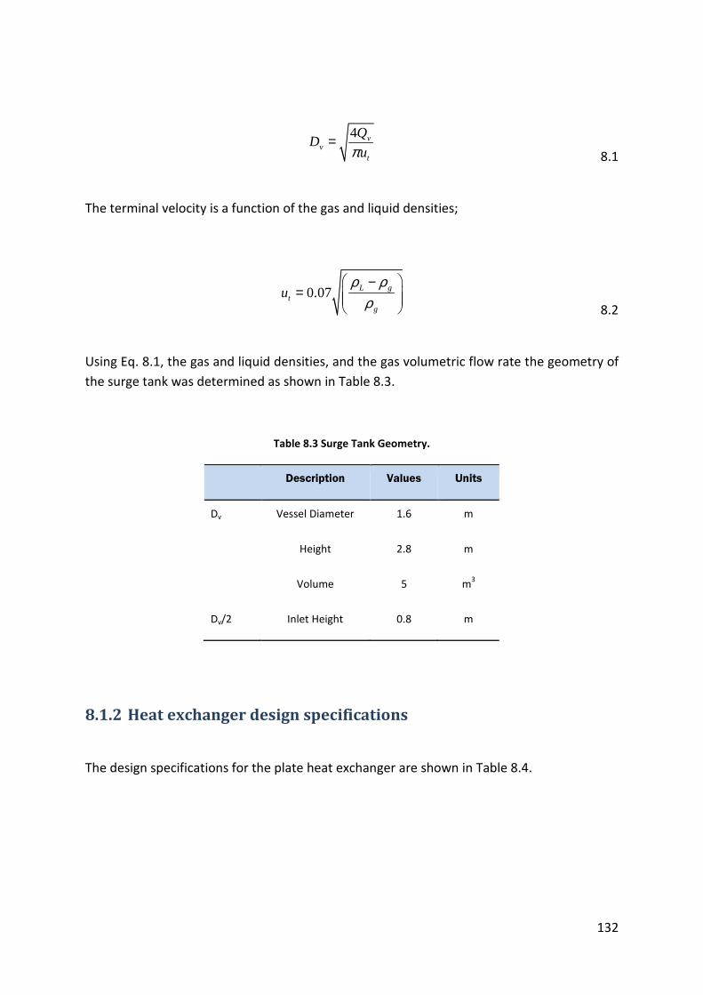
132

The terminal velocity is a function of the gas and liquid densities;

Using Eq. 8.1, the gas and liquid densities, and the gas volumetric flow rate the geometry of

the surge tank was determined as shown in Table 8.3.

Table 8.3 Surge Tank Geometry.

Description Values Units

Dv Vessel Diameter 1.6 m

Height 2.8 m

Volume 5 m3

Dv/2 Inlet Height 0.8 m

8.1.2 Heat exchanger design specifications

The design specifications for the plate heat exchanger are shown in Table 8.4.

4 vv

t

QD

uπ=

8.1

0.07 L gt

g

uρ ρ

ρ −

=

8.2

133

Table 8.4 Heat Exchanger Design Specifications.

Description

Inlet

Temperature

[°C]

Outlet

Temperature

[°C]

Flow

[kg/s]

Flow

[m3/h]

Liquid Side (Based

on Water) 25.7 25 5.5 20

Cooling Water

Side 20 22 2.1 8

Design Conditions

Heat Exchanger Type Plate

Operating temperature range 20 - 85 ºC

Inlet and Outlet Pipe diameters 2 in.

Maximum Pressure Drop 2 bar gauge

Maximum Pressure 6/7.5 bar gauge

Materials of Construction Stainless Steel 316 with compatible seals

Liquids that will flow through the “liquid” side See Table 3.3

8.2 Sensor design specifications

8.2.1 Venturi design

The correlation in Eq. 8.3, which measures the gas mass flow, was derived from the Euler

equation for compressible flow assuming isothermal conditions (see Eq. 8.4, for the

derivation). This correlation was programmed into the PLC and the output recorded. An

absolute pressure transmitter (PE-102)2 was used to measure P1, and a differential pressure

transmitter (DPE-101) to measure P2. The differential pressure transmitter was used since it

has a higher resolution, sensitivity and accuracy than using another absolute pressure

2 See Figure 3.8

134

transmitter. The advantage of this correlation is that by entering the specific gas constant,

the mass flow is calculated for that specific gas based on the gas temperature (in Kelvin) and

the pressure drop across the venturi.

The physical design of the venturi was obtained from the British Standards Institution (BSI)

section 1.1 (1981) for fluid flow in closed conduits. The sizing, as shown in Figure 8.2, was

done based on the CD (discharge coefficient) curve of the venturi. It was decided to size the

venturi so that the value for CD would equal close to one (0.995) where the CD curve is

almost linear. This, according to the BSI, occurs at a Reynolds number range between 2x105

and 1x106. According to Crowe et al. (2001) (Engineering Fluid Mechanics 7

th edition) the CD

value will range between 1 – 1.02 for this range of Reynolds numbers. The measurements

made by the venturi will be validated in a later section of this dissertation.

Constructing the venturi had its own challenges. To ensure that the surface is smooth and

uniform it had to be machined from solid mild steel grade EN8. Since the lathe in the

department’s workshop can only cut tapered sections shorter than 250mm the venturi had

to be made in sections that were press fitted together. This required and depended on the

skill of the machinist, who executed the task to perfection. The venturi was then electro-

galvanized to protect the surface against corrosion.

1

22 2

2ln

D

PP

G C A PRT

= 8.3

135

Figure 8.2 Physical dimensions of the Venturi.

136

Since the fluid is gas it is compressible and is assumed to be isothermal across the venturi.

The Euler conservation of mass equation will be used to derive the gas mass flow correlation

through a venturi:

2 2 22 1

1

2 2 2 2 2 21

1 1 1 1

222 2 2 2

1 1 1

1

22 2

2 2

1 1

2

2 2

1 1

12 2 2 2 2

2

2 2 1

2

2 2

0

02 2

ln 1 02

2 ln

1

1

1

2 ln

2 ln

2 ln

D

D

D

D

vdP udu

u uvdP

RTv

Pu A P u A

uA P A

P u P ART

P P A

PRT

Pu

P AP A

CP AP A

PG u A C RT A

P

C A P PG RT

RT P

G C A P

ρρ

ρ ρ

+ =

+ + =

=

= =

+ − =

=

−

=

−

= =

=

=

∫

1

2

PP

RT

8.4

137

8.2.2 Sensor specification tables

Table 8.5 Digital differential pressure transmitter specifications.

Sensor Specifications

Make Endress + Hauser

Measuring Range 0 – 10kPa

Turn Down Ratio 15:1

Measuring Accuracy ±0.05%

Maximum Linearity Error ±0.075%

Special Classification ATEX II 2G EEx d IIC T6

Membrane Material 316L

Seal Viton

Output 0 – 20mA

Table 8.6 Digital absolute pressure transmitters.


Make Endress + Hauser

Measuring Range 0 – 200kPa abs

Turn Down Ratio 15:1

Measuring Accuracy ±0.05%

Maximum Linearity Error ±0.075%

Special Classification ATEX II 2G EEx d IIC T6

Membrane Material 316L

138


Fill Fluid Silicone Oil

Output 0 – 20mA

Table 8.7 Liquid flow meter specifications summary.


Make Flomec

Measuring Range 1.8 – 27 m3/h

Zero & Span Adjustable

Analog Output 4 – 20mA

Analog Output Accuracy ±0.25% Full Scale

Special Classification IECEX & ATEX approved, Intrinsically safe RT 12

Table 8.8 Gas mass flow meter specifications summary.


Make Sierra

Type Hot Wire Anemometer

Measuring Range 200 – 2100 kg/h

Analog Output 4 – 20mA

Repeatability ±0.2% Full Scale

139

8.3 HAZOP, Safety interlocks and control philosophy

In order to design the control system with the required safety interlocks, a hazard and

operability study was conducted as shown in Table 8.9.

Table 8.9 Hazard and operability table.

Equipment Gas Blower (E-102)

Intention Supply column (E-201) with gas at required pressure (100-105kPa) and flow

(500 - 3000 m3/h, based on Air)

Line No. 33, 34, 35, 36, 38, 42, 32

Intention transfer gas to column (E-201)

Guide

Word

Deviatio

n Cause Consequences Action

No Flow

RVCV-101 stuck

closed

No flow through

column - weeping

Trigger (FAL-101),

Stop Blower,

inspect RVCV-101

air supply, actuator

to valve

connection,

actuator feedback

Blower motor

failure, Bearing

Temp High,

Excessive Vibration

interlocks

No flow through

column - weeping

Shut system down,

inspect control

loop, Blower

bearing temps and

vibration level

(Trigger Alarms),

blower

motor

140

Duty exceeds blower

motor

size (gas density

high)

No flow through

column - weeping Close RCVC - 101

Less Flow

RVCV-101 stuck Less flow through

column - weeping

Stop Blower,

inspect RVCV-101


to valve

connection,

actuator feedback

Fow Blower Inverter

communication

failure

Less flow through

column - weeping

Restart Inverter,

check inverter

error messages

More Flow

Demister

blocked/flooded

Column Pressure

build-up

Trigger Column

Pressure Alarm

High (PAH-206).

Shut system down,

run cleaning

process through

spray ball if needed

Flow

RVCV-101 stuck Excessive flow -

entrainment

Stop Blower,

inspect RVCV-101


to valve

connection,

actuator feedback

Equipment Distillation Characterization Tray Column (E-201)

Intention Simulating distillation hydrodynamic conditions using an inert gas-liquid

system at atmospheric conditions and 25 degrees C

Line No. 34, 36

Intention Simulate distillation hydrodynamics

141

Guide

Word

Deviatio


No Gas Flow V-102 shut close

and/or V-104 shut

closed

No flow-weeping Open V-102 and/or

V-104

Less Gas

Pressure

V-102 shut close and

V-104 open No flow-weeping

Trigger (PAL-206),

Open valve

More Gas

Pressure V-102 open and V-

104 shut closed

No flow-weeping,

glass in window

sections will crack

Trigger (PAH-206),

stop blower

Equipment Surge/Settling Tank (E-101)

Intention Damp gas pressure fluctuations and settling of liquid droplets

Line No. 30, 31

Intention Load system with gas and maintain system pressure

No Pressure PCV - 102 stuck closed Drop in system pressure

gas leak into the system

which could cause fire

and or explosion

Trigger System

pressure alarm Low

(PAL-102)

Close regulator on gas

bottle, inspect PCV-102

air supply, actuator to

valve

connection, actuator

feedback

Pressure Feed Bottle empty Drop in system pressure

in case of gas leak,

insufficient system

loading

close bottle pressure

regulator valve

Pressure MV-108 open Drop is system pressure,

gas leakage into

environment, fire hazard

Close MV-108,

ventilate are

142

More Pressure PCV-102 stuck open Rise in system pressure Trigger (PAH -102)

close PCV-102 and

bottle pressure

regulator valve, inspect

control valve

Equipment Liquid Pump (E-204)

Intention Circulating liquid @ 2-20m3/h & 4-6 bar via heat exchanger (E-205) through column (E-201)

Line No. 2

Intention Transfer liquid to pump

Guide

Word

Deviatio


No Flow Pump stoped, valves

switched to closed lines,

low liquid level in sump

No Flow, possible

pump cavitation and rise

in liquid temp

Trigger FAL-201, stop

pump (E-204),

re-fill liquid sump

Less Flow Strainer blocked, low

liquid level in sump


pump (E-204),

clean strainer, re-fill

liquid sump

Line No. 3

Intention transfer liquid to heat exchanger (E-205)

Guide

Word

Deviatio


No Flow Strainer blocked, or PCV-

205 stuck close, or

manual valves closed

Liquid temp & pressure

build-up in pump


pump (E-204),

clean strainer

Flow meter (FE-201)

rotor

failure

Liquid temp & pressure

build-up in pump


pump (E-204),

open flow meter,

inspect strainer

143

Pump (P-201) failure - Trigger FAL-201, stop

pump (E-204),

inspect control loop

and pump.

Line No. 4

Intention Transfer liquid to heat exchanger (E-205)

Guide

Word

Deviatio


No Flow PCV-205 stuck closed Liquid temp & pressure

build-up in pump


pump (E-204),

use bypass line 21,

inspect valve

More Flow PCV-205 stuck open Flooding of column Trigger FAH-201,

reduce inverter

frequency, inspect

valve

Equipment Liquid Heat Exchanger (E-205)

Intention Control liquid temperature

Line No. 23, 24

Intention Supply heating or cooling water to heat exchanger

Guide

Word

Deviatio


Less Flow cooling water flow too

low due to, cooling

tower operation failed,

or

blocked strainer, or

control valve

failure

Liquid temp build-up Trigger TAH-201, stop

pump (E-204),

inspect strainer,

cooling tower outlet

temp, cooling line

control valve

144

8.3.1 Safety interlocks

The following safety interlocks, see Table 8.10, were made based on the HAZOP study and

equipment failure protection;

Table 8.10 Control system interlocks.

Equipment Monitor If Action

Blower ( E-102)

[37kW motor]

Bearing temp

Axle Vibration

Motor Current

> 70°C

> 7 mm/s

> 64 Amps

Stop Motor

Stop Motor

Close RVCV-

101,

Stop Motor,

Trigger alarm

Pump (E-204)

[5.5kW motor]

Motor Load

liquid flow rate

too high

< 2m3/h

Stop Pump

Stop Pump

Column (E-201) Pressure > 110kPa

>115kPa

< 98kPa

<95kPa

Close PCV-

107,

stop blower

Open PCV-107

Stop blower

Surge Tank (E-101) Pressure < 96kPa

<93kPa

Open PCV-107

Stop blower

Hot Water Bath

(E-301)

Level too low Disable

heating

elements

145

8.3.2 Control philosophy

Table 8.11 Pilot plant control philosophy.

Controlled

Variable

Manipulative Variable Type of Control

TI-201

(Column

Temperature)

CV-301 (Heating)

CV-302 (Cooling)

PV-303 (Select between heating &

cooling lines)

Continuous PID

Continuous PID

Switch, comparative control

TI-301 Heating Elements (TY-301) Continuous PID

FI-201

(Liquid Flow

Rate)

PCV-205

SC-201 (Motor Frequency)

Continuous

PID

Set point

FIR-101

(Gas Flow

Rate)

RVCV-101

SC-105 (Motor Frequency)

Fixed Setting

Set Point

FIR-207

(Weeping

Sampling)

PV-214

PV-216

PV-201

Comparative Automation

FIR-208

(Entrainment

Sampling)

PV-213

PV-215

PV-201

Comparative Automation

146

8.4 Verification of the experimental setup

8.4.1 Calibrating and commissioning of the control system

After construction and installation of the control panel was completed the following steps

were taken to commission the control system:

1. The analog channels of the PLC were calibrated

2. Automation sequences were tested

3. The interlocks were tested

4. Testing equipment operation

8.4.1.1 Calibrating the analog channels

The function of the analog channels is to convert the analog signals from the sensors to

digital values and visa versa. To calibrate each channel the channel gain and offset was

changed so that the converted digital value represented the sensor measurement value.

CALOG – PRO and the CALOG – TEMP calibrators were used to verify the accuracy of the

analog to digital, and digital to analog conversions. Table 8.12 and Table 8.13 provide more

information regarding the measuring and sourcing specifications of the two calibrators.

Table 8.12 The CALOG – PRO specifications.

Measuring Analog Input

Ranges

Accuracy [%] Resolution

0 – 24mA 0.01 1µA

0 – 32V 0.005 1mV

-10 – 100mV 0.005 1µV

0.5 – 100Hz 0.001 0.1Hz

1 – 20 000Hz 0.001 1Hz

147

Sourcing Analog Output

Ranges


0 – 24mA 0.01 1µA

0 – 12V 0.01 1mV

Table 8.13 The CALOG – TEMP specifications.

Measuring Analog Input

Ranges


0 – 24mA 0.02 FS 1µA

-10 – 100mV 0.01 FS 1µV

RTD Type Pt 100 0.05 FS 0.01°C

Sourcing Analog Output

Ranges


0 – 24mA 0.02 FS 1µA

-10 – 100mV 0.01 FS 1µV

RTD Type Pt 100 0.05 FS 0.01°C

8.4.1.2 Testing automation sequences

There are only two automation sequences namely the measurement of the entrainment and

weeping rates. The automation sequence was first tested by simulating the measuring

procedure. Artificial values were entered into the algorithm to test and adjust the

functionality. After all the equipment and utilities were tested a water run was completed to

fully test the automation sequence.

8.4.1.3 Testing interlocks

All the safety interlocks in the software were tested with artificial values, which represented

the system parameters, and by simulating failure conditions. To simulate failure conditions

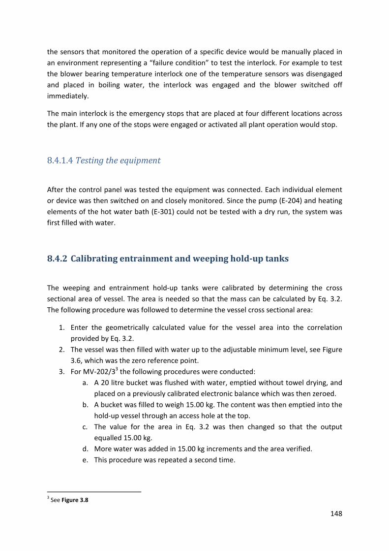
148

the sensors that monitored the operation of a specific device would be manually placed in

an environment representing a “failure condition” to test the interlock. For example to test

the blower bearing temperature interlock one of the temperature sensors was disengaged

and placed in boiling water, the interlock was engaged and the blower switched off

immediately.

The main interlock is the emergency stops that are placed at four different locations across

the plant. If any one of the stops were engaged or activated all plant operation would stop.

8.4.1.4 Testing the equipment

After the control panel was tested the equipment was connected. Each individual element

or device was then switched on and closely monitored. Since the pump (E-204) and heating

elements of the hot water bath (E-301) could not be tested with a dry run, the system was

first filled with water.

8.4.2 Calibrating entrainment and weeping hold-up tanks

The weeping and entrainment hold-up tanks were calibrated by determining the cross

sectional area of vessel. The area is needed so that the mass can be calculated by Eq. 3.2.

The following procedure was followed to determine the vessel cross sectional area:

1. Enter the geometrically calculated value for the vessel area into the correlation

provided by Eq. 3.2.

2. The vessel was then filled with water up to the adjustable minimum level, see Figure

3.6, which was the zero reference point.

3. For MV-202/33 the following procedures were conducted:

a. A 20 litre bucket was flushed with water, emptied without towel drying, and

placed on a previously calibrated electronic balance which was then zeroed.

b. A bucket was filled to weigh 15.00 kg. The content was then emptied into the

hold-up vessel through an access hole at the top.

c. The value for the area in Eq. 3.2 was then changed so that the output

equalled 15.00 kg.

d. More water was added in 15.00 kg increments and the area verified.

e. This procedure was repeated a second time.

3 See Figure 3.8

149

f. The final verification was done by adding 3 volumes of 15.00 kg into the hold-

up vessels (MV-202/3)

4. For the smaller entrainment hold-up vessel (MV-204):

a. A 5 litre bucket was flushed with water, emptied without towel drying, and

placed on a previously calibrated electronic balance which was then zeroed.

b. The bucket was then filled to weigh 4.00 kg. The content was emptied into

the hold-up vessel through an access hole at the top.

c. The value for the area in Eq. 3.2 was then changed so that the output

equalled 4.00 kg.

d. This procedure was repeated a three times.

e. To test and verify the linearity of the vessel area a water mass of 2.00 kg was

added and it was found that the area required stayed constant.

Table 8.14 and Table 8.13 show the measuring accuracy of the hold-up vessels. From

Table 8.14 it can be seen that the measurement accuracy for MV-202/3 is approximately

0.2% excluding the 0.5% accuracy of the PLC analog to digital conversion chart. The

measurement accuracy for MV-204 is approximately 0.5% excluding the accuracy of the

PLC conversion which is another 0.5%.

Table 8.14 Calibration results for the hold-up vessels (MV-202/3).

Description Actual Deviation

Mass Added 15.00 kg ±0.03 kg



Table 8.15 Calibration results for the hold-up vessel (MV-204).

Description Actual Deviation




150

Table 8.16 Calibrated area results for the hold-up vessels (MV-202/3/4).

Description Area

[mm2]

MV-202 123200

MV-203 123300

MV-204 12300

8.4.3 Testing system for leakages

To test the system for leakages compressed air was fed to the system through PCV-107 (the

gas pressure control valve) and soap water was sprayed on all the surfaces and joints. Main

leakages were found at the blower shaft seal and the window sections. After most of the

leakages were sealed the system was then placed under a maximum pressure of 10kPa

gage. Modifications were made to the blower shaft seal and gas leakage was drastically

reduced. It was impossible to find a shaft seal for the blower that would be able to maintain

a complete seal. It was therefore decided to operate the system just above, +5kPa,

atmospheric pressure when using gasses other than air.

8.4.4 Verification of sensor measurements

The aim of this part of the work was to verify if the sensor measurements were realistic and

the methods used for verification provided approximate “ball park” values.

8.4.4.1 Calibrating the venturi flow meter

The venturi measurements were verified using a Pitot tube. Velocity profiles, using Eq. 3.2

and the pressure drop across the Pitot tube, were developed for four different air mass flow

rates on the method shown in Figure 8.3.

2 PV

ρ∆=

8.5

151

The velocity profiles were determined by moving the Pitot tube in 6 increments from the

pipe wall to the pipe centre. The air density was determined using a calibrated digital

absolute pressure transmitter measuring the absolute air pressure 1m behind the Pitot

tube.

Figure 8.3 Velocity profile across a pipe section.

The velocity profiles were then used to develop Figure 8.4. The area under the graph is used

to determine the average air volumetric and mass flow rates based on Eq. 8.6;

Figure 8.4 The area under the graph method was used to determine the average volumetric flow rate across

the gas pipeline for each volumetric flow rate.

2πrdrV

0.00

1.00

2.00

3.00

4.00

5.00

6.00

0.000 0.010 0.020 0.030 0.040 0.050 0.060 0.070 0.080 0.090 0.100

2.π

.r.v

Distance From Tube Centre [m]

.

2 .m V r drρ π= ∫ 8.6

152

Table 8.17 shows the comparative results for the venturi with a CD value of one with that of

the Pitot tube:

Table 8.17 Verification of venturi measurements.

Pitot Tube

[kg/h]

Venturi

[kg/h]

Pitot Tube

over

Venturi

831 848 0.98

1118 1130 0.99

1393 1430 0.97

2010 2010 1.00

The measurements made with the Pitot tube was only used as verification of the venturi

flow rates.

8.4.4.2 Liquid flow meter

The liquid flow meter measurement was verified by measuring a change in the sump volume

over time. To do this the sump level was monitored through a level indicator (sight glass)

while the water was pumped into the draining system. Since the sump cross sectional area

and change in liquid level could be measured the sampling volume was determined. A stop

watch was used to measure the sampling time.

Table 8.18 Liquid flow meter measurement verification.

Sample Volume

[litres]

Sampling

Time

Calculated flow

measurement

[m3/h]

Flow meter

measurement

[m3/h]

99.1 65.0 5.49 5.48

99.1 23.1 15.44 15.70

153

Some difficulty was experienced determining the high flow rate since the liquid level in the

sump oscillated. The result however confirmed that the liquid flow meter measurements

were accurate to an order of magnitude.

8.4.4.3 Differential pressure transmitters

The digital differential pressure transmitter measurements were verified without any

pressure drop by opening both pressure tapings to the atmosphere to determine the zero

point. The max pressure drop of 4kPa was verified by filling a flexible tube with water and

elevating it so that the water level is approximately 408 mm above the centre line of the

device.

The height was determined with a tape measure and is therefore only an approximation.

8.4.4.4 Temperature sensors

The temperature sensor measurements were verified by using the Calog calibrator over a

range of 20 - 90°C. The temperature measurements were found to be ±1°C accurate.

8.4.5 Testing the system with Air and Water

After the all the sensor measurements and functionality was verified the system was filled

with water and the first runs were conducted. The experimental method and the method

the data was acquired will be covered in more detail in a later section of this dissertation.

8.4.5.1 Verify system repeatability

Table 8.19 will give an indication of the expected measurement accuracies of the various

parameters. The gas mass flow measurement accuracy is calculated in Table 8.20.

154

Table 8.19 Calculated measurement accuracies.

Parameter Measurement Accuracy Maximum Deviation

Entrained Liquid L’

±0.5% MV-202/4 + ±0.5% PLC

0.01×30kg= 0.3kg

Liquid Flow Rate

L

±0.25% MV-202/4 + ±0.5% PLC

0.0075×20m3/h = 0.15m

3/h

Gas Mass Flow Rate [kg/h]

see Table 8.20

-0.25% P1&P2, -0.2 [CD], -1°C [T]

(2044-2002)/2044 = 2%

Cp [m/s] ±2% From Venturi 0.02×4m/s = 0.08m/s

The gas mass flow accuracy was calculated entering the maximum deviated value for each

of the parameters required to calculate the mass flow into Eq. 8.3. The maximum expected

deviation was then calculated by comparing the result that does not consider deviation with

the result that does as shown in Table 8.19.

Table 8.20 Calculating maximum deviation expected from venturi mass flow meter using Eq. 8.3.

Parameter Value Deviation Value with

maximum deviation

CD [-] 1.02 -0.02 1

P1 [Pa] 101440 -0.25% 101186

P2 [Pa] 99250 -0.25% 99002

T [K] 298.2 -1°C 297.2

G [kg/h] 2044 2002

To verify the system repeatability, data was generated on four different days at the same

liquid flow rate. Figure 8.5 shows that the data generated at four different dates follow the

same trend for the percentage liquid entrained against the capacity factor (based on the

perforation area).

155

Figure 8.5 Entrainment data collected at four different dates for a liquid flow rate of 57.3 m3/(h.m).

To prove that the entrainment data sampling order does not affect the generated results

data was recorded systematically (see Figure 8.5) for different gas superficial velocities.

0%

5%

10%

15%

20%

25%

30%

4.00 4.10 4.20 4.30 4.40 4.50 4.60 4.70 4.80 4.90

L'/L

Cp[m/s]

21-Jan-09

30-Jan-09

04-Feb-09

30-Mar-09

156

8.5 Experimental data for air water at 25°C

The raw experimental data will be presented in the tables (Table 8.21 to Table 8.28) to follow:

Table 8.21 Experimental entrainment data for 17.2 m3/(h.m) setting and Aesc = 3.33×10

-3 m

2.

ρρρρl [kg/m 3]

ρρρρv [kg/m 3]

An [m 2]

Aesc [m 2]

Liquid Flow [m 3/h]

uL [m/s]

QL [m 3/h.m]

Gas Flow [kg/h]

us [m/s]

L [kg/s]

L' [kg/s]

L'/L [%]

L'/G [%]

Cp

[m/s]

997 1.18 9.538E-02 3.330E-03 2.97 0.248 16.99 1364.05 3.38 0.82 0.04 5.10% 11.09% 0.121

997 1.18 9.538E-02 3.330E-03 2.99 0.249 17.07 1369.19 3.39 0.83 0.04 5.32% 11.58% 0.121

997 1.18 9.538E-02 3.330E-03 2.97 0.248 16.96 1373.22 3.40 0.82 0.05 5.52% 11.90% 0.121

997 1.18 9.538E-02 3.330E-03 2.98 0.249 17.05 1439.82 3.56 0.83 0.06 7.72% 15.94% 0.127

997 1.18 9.538E-02 3.330E-03 2.98 0.249 17.05 1445.09 3.57 0.83 0.07 8.25% 16.98% 0.127

997 1.18 9.538E-02 3.330E-03 2.98 0.249 17.04 1449.56 3.57 0.83 0.07 8.27% 16.96% 0.128

997 1.17 9.538E-02 3.330E-03 3.04 0.254 17.37 1585.85 3.94 0.84 0.18 21.40% 40.91% 0.140

997 1.17 9.538E-02 3.330E-03 3.02 0.252 17.29 1589.13 3.95 0.84 0.18 21.76% 41.29% 0.141

997 1.17 9.538E-02 3.330E-03 3.00 0.250 17.15 1590.43 3.95 0.83 0.19 22.81% 42.93% 0.141

997 1.17 9.538E-02 3.330E-03 3.05 0.254 17.43 1672.36 4.15 0.84 0.37 43.42% 78.96% 0.148

997 1.17 9.538E-02 3.330E-03 3.04 0.253 17.36 1673.36 4.16 0.84 0.37 44.07% 79.79% 0.148

997 1.17 9.538E-02 3.330E-03 3.04 0.254 17.37 1675.70 4.16 0.84 0.38 45.38% 82.10% 0.148

997 1.17 9.538E-02 3.330E-03 3.05 0.254 17.41 1672.24 4.15 0.84 0.38 45.46% 82.59% 0.148

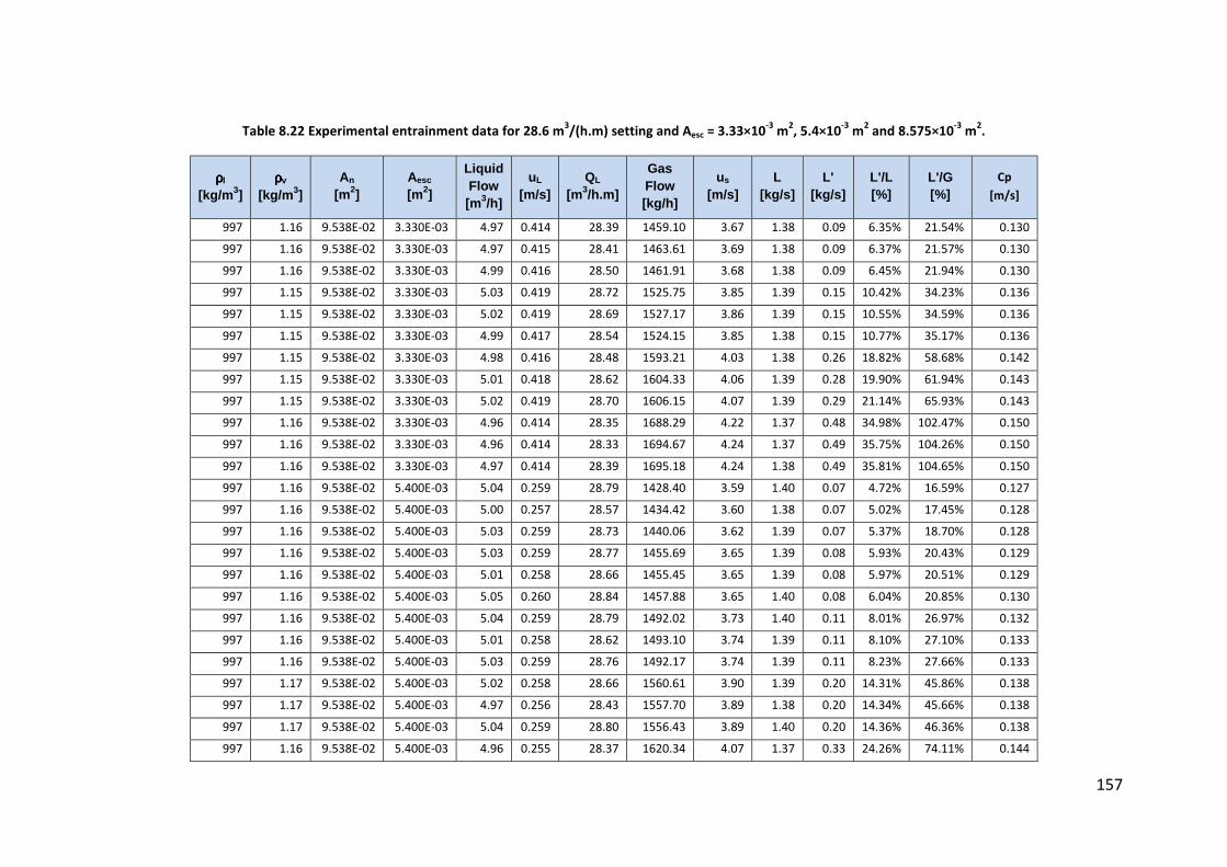
157


-3 m

2, 5.4×10

-3 m

2 and 8.575×10

-3 m

2.

ρρρρl [kg/m 3]

ρρρρv [kg/m 3]

An [m 2]

Aesc [m 2]

Liquid Flow [m 3/h]

uL [m/s]

QL [m 3/h.m]

Gas Flow [kg/h]

us [m/s]

L [kg/s]

L' [kg/s]

L'/L [%]

L'/G [%]

Cp

[m/s]

997 1.16 9.538E-02 3.330E-03 4.97 0.414 28.39 1459.10 3.67 1.38 0.09 6.35% 21.54% 0.130

997 1.16 9.538E-02 3.330E-03 4.97 0.415 28.41 1463.61 3.69 1.38 0.09 6.37% 21.57% 0.130

997 1.16 9.538E-02 3.330E-03 4.99 0.416 28.50 1461.91 3.68 1.38 0.09 6.45% 21.94% 0.130

997 1.15 9.538E-02 3.330E-03 5.03 0.419 28.72 1525.75 3.85 1.39 0.15 10.42% 34.23% 0.136

997 1.15 9.538E-02 3.330E-03 5.02 0.419 28.69 1527.17 3.86 1.39 0.15 10.55% 34.59% 0.136

997 1.15 9.538E-02 3.330E-03 4.99 0.417 28.54 1524.15 3.85 1.38 0.15 10.77% 35.17% 0.136

997 1.15 9.538E-02 3.330E-03 4.98 0.416 28.48 1593.21 4.03 1.38 0.26 18.82% 58.68% 0.142

997 1.15 9.538E-02 3.330E-03 5.01 0.418 28.62 1604.33 4.06 1.39 0.28 19.90% 61.94% 0.143

997 1.15 9.538E-02 3.330E-03 5.02 0.419 28.70 1606.15 4.07 1.39 0.29 21.14% 65.93% 0.143

997 1.16 9.538E-02 3.330E-03 4.96 0.414 28.35 1688.29 4.22 1.37 0.48 34.98% 102.47% 0.150

997 1.16 9.538E-02 3.330E-03 4.96 0.414 28.33 1694.67 4.24 1.37 0.49 35.75% 104.26% 0.150

997 1.16 9.538E-02 3.330E-03 4.97 0.414 28.39 1695.18 4.24 1.38 0.49 35.81% 104.65% 0.150

997 1.16 9.538E-02 5.400E-03 5.04 0.259 28.79 1428.40 3.59 1.40 0.07 4.72% 16.59% 0.127

997 1.16 9.538E-02 5.400E-03 5.00 0.257 28.57 1434.42 3.60 1.38 0.07 5.02% 17.45% 0.128

997 1.16 9.538E-02 5.400E-03 5.03 0.259 28.73 1440.06 3.62 1.39 0.07 5.37% 18.70% 0.128

997 1.16 9.538E-02 5.400E-03 5.03 0.259 28.77 1455.69 3.65 1.39 0.08 5.93% 20.43% 0.129

997 1.16 9.538E-02 5.400E-03 5.01 0.258 28.66 1455.45 3.65 1.39 0.08 5.97% 20.51% 0.129

997 1.16 9.538E-02 5.400E-03 5.05 0.260 28.84 1457.88 3.65 1.40 0.08 6.04% 20.85% 0.130

997 1.16 9.538E-02 5.400E-03 5.04 0.259 28.79 1492.02 3.73 1.40 0.11 8.01% 26.97% 0.132

997 1.16 9.538E-02 5.400E-03 5.01 0.258 28.62 1493.10 3.74 1.39 0.11 8.10% 27.10% 0.133

997 1.16 9.538E-02 5.400E-03 5.03 0.259 28.76 1492.17 3.74 1.39 0.11 8.23% 27.66% 0.133

997 1.17 9.538E-02 5.400E-03 5.02 0.258 28.66 1560.61 3.90 1.39 0.20 14.31% 45.86% 0.138

997 1.17 9.538E-02 5.400E-03 4.97 0.256 28.43 1557.70 3.89 1.38 0.20 14.34% 45.66% 0.138

997 1.17 9.538E-02 5.400E-03 5.04 0.259 28.80 1556.43 3.89 1.40 0.20 14.36% 46.36% 0.138

997 1.16 9.538E-02 5.400E-03 4.96 0.255 28.37 1620.34 4.07 1.37 0.33 24.26% 74.11% 0.144

158


-3 m

2, 5.4×10

-3 m

2 and 8.575×10

-3 m

2.

ρρρρl [kg/m 3]

ρρρρv [kg/m 3]

An [m 2]

Aesc [m 2]

Liquid Flow [m 3/h]

uL [m/s]

QL [m 3/h.m]

Gas Flow [kg/h]

us [m/s]

L [kg/s]

L' [kg/s]

L'/L [%]

L'/G [%]

Cp

[m/s]

997 1.16 9.538E-02 5.400E-03 4.98 0.256 28.43 1622.29 4.08 1.38 0.34 24.83% 75.92% 0.144

997 1.16 9.538E-02 5.400E-03 4.98 0.256 28.47 1623.37 4.08 1.38 0.35 25.21% 77.15% 0.144

997 1.16 9.538E-02 5.400E-03 4.97 0.256 28.42 1671.39 4.19 1.38 0.45 32.64% 96.84% 0.148

997 1.16 9.538E-02 5.400E-03 4.97 0.256 28.42 1674.77 4.20 1.38 0.45 32.97% 97.62% 0.149

997 1.16 9.538E-02 5.400E-03 4.97 0.256 28.41 1677.52 4.21 1.38 0.45 33.02% 97.55% 0.149

997 1.16 9.538E-02 5.400E-03 4.97 0.256 28.41 1681.83 4.22 1.38 0.46 33.24% 97.98% 0.149

997 1.17 9.538E-02 8.575E-03 5.02 0.163 28.69 1591.68 3.97 1.39 0.16 11.26% 35.40% 0.141

997 1.16 9.538E-02 8.575E-03 5.02 0.163 28.71 1599.74 4.00 1.39 0.18 13.07% 40.91% 0.142

997 1.17 9.538E-02 8.575E-03 5.02 0.163 28.70 1606.67 4.00 1.39 0.19 13.62% 42.45% 0.142

997 1.17 9.538E-02 8.575E-03 5.02 0.162 28.66 1605.86 4.01 1.39 0.19 13.81% 42.99% 0.142

997 1.17 9.538E-02 8.575E-03 4.95 0.160 28.27 1611.13 4.01 1.37 0.19 13.82% 42.31% 0.143

997 1.16 9.538E-02 8.575E-03 5.01 0.162 28.65 1742.83 4.36 1.39 0.45 32.23% 92.43% 0.155

997 1.16 9.538E-02 8.575E-03 5.02 0.163 28.69 1742.72 4.36 1.39 0.45 32.24% 92.59% 0.155

997 1.16 9.538E-02 8.575E-03 5.03 0.163 28.73 1748.93 4.38 1.39 0.46 33.09% 94.86% 0.155

997 1.17 9.538E-02 8.575E-03 5.02 0.163 28.67 1748.57 4.37 1.39 0.46 33.45% 95.68% 0.155

997 1.16 9.538E-02 8.575E-03 5.00 0.162 28.59 1835.06 4.59 1.39 0.65 46.72% 127.00% 0.163

997 1.16 9.538E-02 8.575E-03 5.03 0.163 28.73 1844.21 4.62 1.39 0.66 47.23% 128.37% 0.164

997 1.16 9.538E-02 8.575E-03 5.00 0.162 28.58 1842.11 4.61 1.38 0.66 47.53% 128.64% 0.164

997 1.16 9.538E-02 8.575E-03 5.02 0.162 28.66 1848.92 4.64 1.39 0.69 49.74% 134.51% 0.164

159

Table 8.23 Experimental entrainment data for 40 m3/(h.m) setting and Aesc = 3.33×10

-3 m

2, 5.4×10

-3 m

2 and 8.575×10

-3 m

2.

ρρρρl [kg/m 3]

ρρρρv [kg/m 3]

An [m 2]

Aesc [m 2]

Liquid Flow [m 3/h]

uL [m/s]

QL [m 3/h.m]

Gas Flow [kg/h]

us [m/s]

L [kg/s]

L' [kg/s]

L'/L [%]

L'/G [%]

Cp

[m/s]

997 1.18 9.538E-02 3.330E-03 7.01 0.585 40.05 1546.75 3.83 1.94 0.10 4.95% 22.38% 0.137

997 1.18 9.538E-02 3.330E-03 6.98 0.582 39.89 1553.34 3.84 1.93 0.10 5.29% 23.71% 0.137

997 1.18 9.538E-02 3.330E-03 7.01 0.585 40.07 1553.17 3.85 1.94 0.11 5.49% 24.70% 0.137

997 1.17 9.538E-02 3.330E-03 6.99 0.583 39.96 1638.15 4.06 1.94 0.21 10.62% 45.23% 0.145

997 1.17 9.538E-02 3.330E-03 7.04 0.587 40.20 1635.73 4.06 1.95 0.21 10.66% 45.71% 0.145

997 1.17 9.538E-02 3.330E-03 7.03 0.587 40.18 1643.11 4.08 1.95 0.21 10.85% 46.28% 0.145

997 1.17 9.538E-02 3.330E-03 7.02 0.586 40.12 1637.80 4.07 1.94 0.21 10.90% 46.58% 0.145

997 1.17 9.538E-02 3.330E-03 7.03 0.586 40.15 1703.24 4.25 1.95 0.34 17.71% 72.81% 0.151

997 1.17 9.538E-02 3.330E-03 7.02 0.586 40.13 1704.25 4.25 1.95 0.35 17.97% 73.82% 0.151

997 1.17 9.538E-02 3.330E-03 6.99 0.583 39.94 1706.24 4.25 1.94 0.35 18.25% 74.52% 0.151

997 1.17 9.538E-02 3.330E-03 6.99 0.583 39.96 1772.36 4.41 1.94 0.49 25.48% 100.22% 0.157

997 1.17 9.538E-02 3.330E-03 6.99 0.583 39.92 1778.47 4.42 1.93 0.50 25.97% 101.72% 0.157

997 1.17 9.538E-02 3.330E-03 6.98 0.582 39.88 1780.31 4.42 1.93 0.51 26.64% 104.12% 0.157

997 1.18 9.538E-02 5.400E-03 7.01 0.360 40.03 1517.88 3.75 1.94 0.09 4.51% 20.73% 0.134

997 1.18 9.538E-02 5.400E-03 7.01 0.361 40.05 1522.32 3.76 1.94 0.09 4.57% 20.99% 0.134

997 1.18 9.538E-02 5.400E-03 7.00 0.360 40.00 1528.24 3.76 1.94 0.09 4.73% 21.62% 0.135

997 1.16 9.538E-02 5.400E-03 7.05 0.363 40.30 1602.50 4.01 1.95 0.18 9.30% 40.82% 0.142

997 1.16 9.538E-02 5.400E-03 7.03 0.362 40.18 1599.72 4.00 1.95 0.19 9.52% 41.71% 0.142

997 1.16 9.538E-02 5.400E-03 7.02 0.361 40.09 1603.58 4.01 1.94 0.19 9.53% 41.58% 0.142

997 1.17 9.538E-02 5.400E-03 6.95 0.358 39.73 1660.56 4.15 1.93 0.28 14.41% 60.16% 0.147

997 1.17 9.538E-02 5.400E-03 7.03 0.362 40.19 1663.96 4.16 1.95 0.29 14.79% 62.35% 0.148

997 1.17 9.538E-02 5.400E-03 7.02 0.361 40.12 1667.85 4.17 1.94 0.29 14.99% 62.92% 0.148

997 1.16 9.538E-02 5.400E-03 7.03 0.362 40.20 1774.79 4.44 1.95 0.52 26.75% 105.72% 0.158

997 1.17 9.538E-02 5.400E-03 6.98 0.359 39.87 1773.00 4.43 1.93 0.54 27.86% 109.30% 0.157

997 1.16 9.538E-02 5.400E-03 7.01 0.361 40.08 1775.60 4.44 1.94 0.55 28.24% 111.23% 0.158

160


-3 m

2, 5.4×10

-3 m

2 and 8.575×10

-3 m

2.

ρρρρl [kg/m 3]

ρρρρv [kg/m 3]

An [m 2]

Aesc [m 2]

Liquid Flow [m 3/h]

uL [m/s]

QL [m 3/h.m]

Gas Flow [kg/h]

us [m/s]

L [kg/s]

L' [kg/s]

L'/L [%]

L'/G [%]

Cp

[m/s]

997 1.19 9.538E-02 8.575E-03 7.00 0.227 40.00 1495.15 3.67 1.94 0.05 2.83% 13.22% 0.132

997 1.19 9.538E-02 8.575E-03 7.00 0.227 40.00 1508.54 3.70 1.94 0.06 2.96% 13.70% 0.133

997 1.18 9.538E-02 8.575E-03 7.02 0.227 40.11 1518.01 3.75 1.94 0.07 3.60% 16.61% 0.134

997 1.18 9.538E-02 8.575E-03 7.02 0.227 40.12 1521.50 3.76 1.94 0.07 3.67% 16.90% 0.134

997 1.18 9.538E-02 8.575E-03 6.98 0.226 39.86 1526.12 3.76 1.93 0.07 3.81% 17.37% 0.135

997 1.18 9.538E-02 8.575E-03 7.02 0.227 40.12 1532.12 3.77 1.94 0.08 3.88% 17.72% 0.135

997 1.19 9.538E-02 8.575E-03 7.02 0.227 40.12 1541.88 3.79 1.94 0.08 4.13% 18.74% 0.136

997 1.15 9.538E-02 8.575E-03 6.95 0.225 39.70 1545.25 3.90 1.92 0.10 4.98% 22.33% 0.138

997 1.18 9.538E-02 8.575E-03 7.05 0.228 40.28 1633.29 4.04 1.95 0.21 10.71% 46.08% 0.144

997 1.17 9.538E-02 8.575E-03 7.02 0.227 40.12 1635.32 4.06 1.94 0.21 10.80% 46.21% 0.145

997 1.17 9.538E-02 8.575E-03 7.01 0.227 40.04 1630.48 4.06 1.94 0.21 10.82% 46.36% 0.144

997 1.17 9.538E-02 8.575E-03 7.02 0.227 40.10 1634.12 4.07 1.94 0.21 10.96% 46.93% 0.145

997 1.17 9.538E-02 8.575E-03 7.03 0.228 40.16 1636.38 4.06 1.95 0.21 10.98% 47.00% 0.145

997 1.17 9.538E-02 8.575E-03 7.04 0.228 40.22 1638.50 4.06 1.95 0.22 11.38% 48.73% 0.145

997 1.16 9.538E-02 8.575E-03 7.01 0.227 40.05 1656.29 4.15 1.94 0.28 14.63% 61.72% 0.147

997 1.16 9.538E-02 8.575E-03 7.02 0.227 40.09 1661.61 4.16 1.94 0.30 15.63% 65.82% 0.148

997 1.16 9.538E-02 8.575E-03 6.99 0.226 39.93 1659.79 4.16 1.94 0.31 16.04% 67.34% 0.147

997 1.17 9.538E-02 8.575E-03 6.99 0.227 39.97 1698.81 4.24 1.94 0.37 19.34% 79.39% 0.151

997 1.17 9.538E-02 8.575E-03 7.03 0.228 40.15 1706.06 4.25 1.95 0.38 19.63% 80.59% 0.151

997 1.17 9.538E-02 8.575E-03 7.04 0.228 40.23 1709.36 4.26 1.95 0.38 19.67% 80.79% 0.151

997 1.17 9.538E-02 8.575E-03 7.01 0.227 40.06 1703.70 4.25 1.94 0.39 19.85% 81.43% 0.151

997 1.16 9.538E-02 8.575E-03 6.97 0.226 39.82 1718.55 4.31 1.93 0.42 21.55% 87.12% 0.153

997 1.16 9.538E-02 8.575E-03 6.96 0.225 39.76 1719.88 4.32 1.93 0.42 21.66% 87.38% 0.153

997 1.16 9.538E-02 8.575E-03 7.01 0.227 40.07 1718.73 4.32 1.94 0.43 21.96% 89.31% 0.153

997 1.16 9.538E-02 8.575E-03 6.99 0.226 39.95 1724.55 4.32 1.94 0.43 22.35% 90.33% 0.153

161


-3 m

2, 5.4×10

-3 m

2 and 8.575×10

-3 m

2.

ρρρρl [kg/m 3]

ρρρρv [kg/m 3]

An [m 2]

Aesc [m 2]

Liquid Flow [m 3/h]

uL [m/s]

QL [m 3/h.m]

Gas Flow [kg/h]

us [m/s]

L [kg/s]

L' [kg/s]

L'/L [%]

L'/G [%]

Cp

[m/s]

997 1.16 9.538E-02 8.575E-03 7.00 0.227 40.01 1723.27 4.32 1.94 0.44 22.44% 90.90% 0.153

997 1.17 9.538E-02 8.575E-03 7.01 0.227 40.05 1769.71 4.42 1.94 0.54 27.78% 109.69% 0.157

997 1.17 9.538E-02 8.575E-03 7.01 0.227 40.08 1767.83 4.42 1.94 0.54 27.82% 110.05% 0.157

997 1.17 9.538E-02 8.575E-03 7.01 0.227 40.07 1775.63 4.43 1.94 0.55 28.12% 110.72% 0.157

997 1.17 9.538E-02 8.575E-03 7.02 0.227 40.11 1772.35 4.42 1.94 0.55 28.19% 111.31% 0.157


-3 m

2 and 8.575×10

-3 m

2.

ρρρρl [kg/m 3]

ρρρρv [kg/m 3]

An [m 2]

Aesc [m 2]

Liquid Flow [m 3/h]

uL [m/s]

QL [m 3/h.m]

Gas Flow [kg/h]

us [m/s]

L [kg/s]

L' [kg/s]

L'/L [%]

L'/G [%]

Cp

[m/s]

997 1.17 9.538E-02 5.400E-03 9.99 0.514 57.10 1595.77 3.98 2.77 0.13 4.81% 30.05% 0.141

997 1.17 9.538E-02 5.400E-03 9.99 0.514 57.11 1600.64 4.00 2.77 0.14 4.96% 30.86% 0.142

997 1.17 9.538E-02 5.400E-03 10.01 0.515 57.20 1602.25 4.00 2.77 0.14 5.17% 32.19% 0.142

997 1.18 9.538E-02 5.400E-03 9.99 0.514 57.11 1673.07 4.14 2.77 0.23 8.23% 49.04% 0.148

997 1.17 9.538E-02 5.400E-03 9.95 0.512 56.83 1709.93 4.24 2.75 0.32 11.63% 67.43% 0.151

997 1.17 9.538E-02 5.400E-03 10.04 0.516 57.35 1707.34 4.24 2.78 0.32 11.55% 67.71% 0.151

997 1.18 9.538E-02 5.400E-03 9.96 0.513 56.93 1718.96 4.26 2.76 0.33 12.04% 69.56% 0.152

997 1.16 9.538E-02 5.400E-03 10.02 0.515 57.26 1754.06 4.39 2.78 0.44 15.75% 89.68% 0.156

997 1.16 9.538E-02 5.400E-03 10.04 0.516 57.36 1757.50 4.40 2.78 0.44 15.75% 89.68% 0.156

997 1.16 9.538E-02 5.400E-03 10.03 0.516 57.32 1758.61 4.40 2.78 0.44 15.92% 90.50% 0.156

997 1.17 9.538E-02 5.400E-03 9.97 0.513 56.97 1819.14 4.54 2.76 0.62 22.29% 121.80% 0.161

997 1.17 9.538E-02 5.400E-03 10.04 0.516 57.37 1818.79 4.54 2.78 0.62 22.39% 123.22% 0.161

997 1.17 9.538E-02 5.400E-03 9.98 0.514 57.05 1823.44 4.54 2.76 0.63 22.78% 124.35% 0.162

162


-3 m

2 and 8.575×10

-3 m

2.

ρρρρl [kg/m 3]

ρρρρv [kg/m 3]

An [m 2]

Aesc [m 2]

Liquid Flow [m 3/h]

uL [m/s]

QL [m 3/h.m]

Gas Flow [kg/h]

us [m/s]

L [kg/s]

L' [kg/s]

L'/L [%]

L'/G [%]

Cp

[m/s]

997 1.15 9.538E-02 8.575E-03 9.98 0.323 57.03 1571.57 3.97 2.76 0.10 3.71% 23.52% 0.140

997 1.15 9.538E-02 8.575E-03 10.00 0.324 57.12 1576.46 3.99 2.77 0.10 3.77% 23.82% 0.141

997 1.15 9.538E-02 8.575E-03 10.01 0.324 57.19 1579.41 3.99 2.77 0.11 3.85% 24.30% 0.141

997 1.15 9.538E-02 8.575E-03 9.98 0.323 57.02 1588.58 4.01 2.76 0.11 4.13% 25.85% 0.142

997 1.16 9.538E-02 8.575E-03 10.00 0.324 57.12 1597.81 4.00 2.77 0.13 4.63% 28.86% 0.142

997 1.16 9.538E-02 8.575E-03 9.99 0.324 57.09 1598.14 4.00 2.77 0.13 4.65% 28.99% 0.142

997 1.16 9.538E-02 8.575E-03 9.90 0.321 56.56 1601.80 4.01 2.74 0.13 4.72% 29.06% 0.142

997 1.16 9.538E-02 8.575E-03 9.99 0.324 57.10 1639.77 4.12 2.77 0.17 6.14% 37.29% 0.146

997 1.16 9.538E-02 8.575E-03 10.09 0.327 57.65 1647.33 4.15 2.79 0.19 6.75% 41.19% 0.147

997 1.15 9.538E-02 8.575E-03 10.14 0.328 57.93 1643.96 4.15 2.81 0.19 6.91% 42.50% 0.147

997 1.16 9.538E-02 8.575E-03 9.89 0.320 56.53 1647.22 4.14 2.74 0.20 7.17% 42.91% 0.147

997 1.16 9.538E-02 8.575E-03 10.01 0.324 57.22 1647.50 4.15 2.77 0.20 7.22% 43.74% 0.147

997 1.17 9.538E-02 8.575E-03 9.99 0.324 57.09 1650.40 4.12 2.77 0.23 8.22% 49.59% 0.146

997 1.17 9.538E-02 8.575E-03 10.00 0.324 57.14 1651.39 4.12 2.77 0.23 8.22% 49.65% 0.146

997 1.17 9.538E-02 8.575E-03 9.95 0.322 56.88 1659.38 4.14 2.76 0.23 8.51% 50.89% 0.147

997 1.15 9.538E-02 8.575E-03 10.14 0.328 57.95 1684.05 4.25 2.81 0.26 9.31% 55.90% 0.150

997 1.15 9.538E-02 8.575E-03 10.07 0.326 57.53 1684.95 4.25 2.79 0.29 10.24% 61.00% 0.150

997 1.15 9.538E-02 8.575E-03 10.06 0.326 57.51 1689.47 4.27 2.79 0.29 10.49% 62.27% 0.151

997 1.15 9.538E-02 8.575E-03 10.05 0.326 57.43 1694.75 4.28 2.78 0.29 10.58% 62.53% 0.151

997 1.17 9.538E-02 8.575E-03 10.02 0.325 57.27 1700.51 4.25 2.78 0.30 10.83% 63.66% 0.151

997 1.17 9.538E-02 8.575E-03 9.98 0.323 57.05 1703.53 4.25 2.76 0.31 11.06% 64.63% 0.151

997 1.15 9.538E-02 8.575E-03 10.01 0.324 57.17 1699.09 4.29 2.77 0.31 11.28% 66.21% 0.152

997 1.16 9.538E-02 8.575E-03 10.05 0.326 57.43 1721.51 4.31 2.78 0.39 13.92% 81.01% 0.153

997 1.17 9.538E-02 8.575E-03 9.98 0.323 57.04 1724.91 4.31 2.76 0.39 14.28% 82.41% 0.153

997 1.16 9.538E-02 8.575E-03 9.99 0.324 57.09 1723.05 4.31 2.77 0.40 14.36% 83.03% 0.153

163


-3 m

2 and 8.575×10

-3 m

2.

ρρρρl [kg/m 3]

ρρρρv [kg/m 3]

An [m 2]

Aesc [m 2]

Liquid Flow [m 3/h]

uL [m/s]

QL [m 3/h.m]

Gas Flow [kg/h]

us [m/s]

L [kg/s]

L' [kg/s]

L'/L [%]

L'/G [%]

Cp

[m/s]

997 1.16 9.538E-02 8.575E-03 9.99 0.324 57.07 1748.87 4.38 2.77 0.42 15.18% 86.44% 0.155

997 1.15 9.538E-02 8.575E-03 10.10 0.327 57.74 1745.67 4.42 2.80 0.42 15.16% 87.49% 0.156

997 1.15 9.538E-02 8.575E-03 10.09 0.327 57.68 1746.59 4.42 2.80 0.43 15.39% 88.68% 0.156

997 1.15 9.538E-02 8.575E-03 10.09 0.327 57.65 1739.22 4.41 2.79 0.43 15.37% 88.89% 0.155

997 1.15 9.538E-02 8.575E-03 10.04 0.325 57.36 1751.74 4.43 2.78 0.43 15.65% 89.39% 0.156

997 1.15 9.538E-02 8.575E-03 10.04 0.325 57.36 1746.95 4.42 2.78 0.44 15.81% 90.58% 0.156

997 1.15 9.538E-02 8.575E-03 10.13 0.328 57.88 1748.46 4.42 2.81 0.44 15.82% 91.40% 0.156

997 1.16 9.538E-02 8.575E-03 10.01 0.324 57.19 1772.95 4.45 2.77 0.49 17.68% 99.50% 0.158

997 1.16 9.538E-02 8.575E-03 9.99 0.324 57.11 1779.02 4.46 2.77 0.49 17.83% 99.90% 0.158

997 1.16 9.538E-02 8.575E-03 10.00 0.324 57.14 1777.88 4.45 2.77 0.50 18.11% 101.57% 0.158

997 1.16 9.538E-02 8.575E-03 10.03 0.325 57.31 1773.49 4.44 2.78 0.50 18.17% 102.46% 0.158

997 1.16 9.538E-02 8.575E-03 10.02 0.324 57.23 1780.45 4.46 2.77 0.51 18.36% 102.96% 0.158

997 1.16 9.538E-02 8.575E-03 10.00 0.324 57.16 1795.49 4.50 2.77 0.59 21.45% 119.13% 0.159

997 1.16 9.538E-02 8.575E-03 9.98 0.323 57.01 1797.49 4.50 2.76 0.61 22.06% 122.10% 0.160

997 1.16 9.538E-02 8.575E-03 9.99 0.324 57.09 1808.88 4.54 2.77 0.63 22.84% 125.79% 0.161

997 1.16 9.538E-02 8.575E-03 10.02 0.325 57.28 1851.61 4.64 2.78 0.73 26.20% 141.39% 0.164

997 1.16 9.538E-02 8.575E-03 10.00 0.324 57.16 1847.61 4.63 2.77 0.74 26.66% 143.90% 0.164

997 1.16 9.538E-02 8.575E-03 10.02 0.325 57.28 1850.88 4.64 2.78 0.75 27.00% 145.78% 0.165

997 1.16 9.538E-02 8.575E-03 9.97 0.323 56.99 1848.77 4.63 2.76 0.75 27.15% 146.03% 0.164

997 1.16 9.538E-02 8.575E-03 10.04 0.325 57.34 1849.57 4.64 2.78 0.75 27.00% 146.04% 0.164

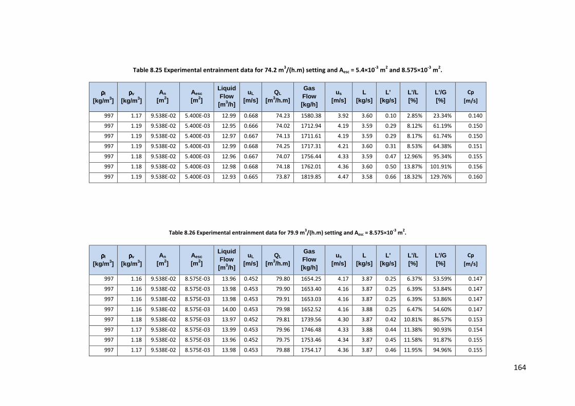
164


-3 m

2 and 8.575×10

-3 m

2.

ρρρρl [kg/m 3]

ρρρρv [kg/m 3]

An [m 2]

Aesc [m 2]

Liquid Flow [m 3/h]

uL [m/s]

QL [m 3/h.m]

Gas Flow [kg/h]

us [m/s]

L [kg/s]

L' [kg/s]

L'/L [%]

L'/G [%]

Cp

[m/s]

997 1.17 9.538E-02 5.400E-03 12.99 0.668 74.23 1580.38 3.92 3.60 0.10 2.85% 23.34% 0.140

997 1.19 9.538E-02 5.400E-03 12.95 0.666 74.02 1712.94 4.19 3.59 0.29 8.12% 61.19% 0.150

997 1.19 9.538E-02 5.400E-03 12.97 0.667 74.13 1711.61 4.19 3.59 0.29 8.17% 61.74% 0.150

997 1.19 9.538E-02 5.400E-03 12.99 0.668 74.25 1717.31 4.21 3.60 0.31 8.53% 64.38% 0.151

997 1.18 9.538E-02 5.400E-03 12.96 0.667 74.07 1756.44 4.33 3.59 0.47 12.96% 95.34% 0.155

997 1.18 9.538E-02 5.400E-03 12.98 0.668 74.18 1762.01 4.36 3.60 0.50 13.87% 101.91% 0.156

997 1.19 9.538E-02 5.400E-03 12.93 0.665 73.87 1819.85 4.47 3.58 0.66 18.32% 129.76% 0.160


-3 m

2.

ρρρρl [kg/m 3]

ρρρρv [kg/m 3]

An [m 2]

Aesc [m 2]

Liquid Flow [m 3/h]

uL [m/s]

QL [m 3/h.m]

Gas Flow [kg/h]

us [m/s]

L [kg/s]

L' [kg/s]

L'/L [%]

L'/G [%]

Cp

[m/s]

997 1.16 9.538E-02 8.575E-03 13.96 0.452 79.80 1654.25 4.17 3.87 0.25 6.37% 53.59% 0.147

997 1.16 9.538E-02 8.575E-03 13.98 0.453 79.90 1653.40 4.16 3.87 0.25 6.39% 53.84% 0.147

997 1.16 9.538E-02 8.575E-03 13.98 0.453 79.91 1653.03 4.16 3.87 0.25 6.39% 53.86% 0.147

997 1.16 9.538E-02 8.575E-03 14.00 0.453 79.98 1652.52 4.16 3.88 0.25 6.47% 54.60% 0.147

997 1.18 9.538E-02 8.575E-03 13.97 0.452 79.81 1739.56 4.30 3.87 0.42 10.81% 86.57% 0.153

997 1.17 9.538E-02 8.575E-03 13.99 0.453 79.96 1746.48 4.33 3.88 0.44 11.38% 90.93% 0.154

997 1.18 9.538E-02 8.575E-03 13.96 0.452 79.75 1753.46 4.34 3.87 0.45 11.58% 91.87% 0.155

997 1.17 9.538E-02 8.575E-03 13.98 0.453 79.88 1754.17 4.36 3.87 0.46 11.95% 94.96% 0.155

165


-3 m

2.

ρρρρl [kg/m 3]

ρρρρv [kg/m 3]

An [m 2]

Aesc [m 2]

Liquid Flow [m 3/h]

uL [m/s]

QL [m 3/h.m]

Gas Flow [kg/h]

us [m/s]

L [kg/s]

L' [kg/s]

L'/L [%]

L'/G [%]

Cp

[m/s]

997 1.17 9.538E-02 8.575E-03 13.95 0.452 79.70 1751.22 4.35 3.86 0.47 12.30% 97.63% 0.155

997 1.17 9.538E-02 8.575E-03 13.95 0.452 79.72 1783.52 4.45 3.86 0.59 15.22% 118.70% 0.158

997 1.17 9.538E-02 8.575E-03 13.93 0.451 79.60 1792.27 4.46 3.86 0.67 17.50% 135.56% 0.159

997 1.17 9.538E-02 8.575E-03 13.99 0.453 79.93 1814.15 4.53 3.87 0.75 19.26% 148.03% 0.161

997 1.16 9.538E-02 8.575E-03 14.00 0.454 80.02 1799.59 4.51 3.88 0.75 19.44% 150.83% 0.160

997 1.17 9.538E-02 8.575E-03 13.97 0.452 79.81 1816.23 4.53 3.87 0.75 19.50% 149.51% 0.161

997 1.16 9.538E-02 8.575E-03 13.99 0.453 79.92 1809.78 4.53 3.87 0.76 19.52% 150.40% 0.161

997 1.16 9.538E-02 8.575E-03 13.98 0.453 79.90 1807.68 4.53 3.87 0.76 19.71% 152.03% 0.161

997 1.17 9.538E-02 8.575E-03 14.02 0.454 80.11 1812.28 4.53 3.88 0.77 19.76% 152.43% 0.161

997 1.17 9.538E-02 8.575E-03 13.97 0.452 79.82 1812.63 4.53 3.87 0.77 19.83% 152.34% 0.161

997 1.16 9.538E-02 8.575E-03 13.97 0.452 79.81 1813.05 4.54 3.87 0.78 20.25% 155.53% 0.161


-3 m

2.

ρρρρl [kg/m 3]

ρρρρv [kg/m 3]

An [m 2]

Aesc [m 2]

Liquid Flow [m 3/h]

uL [m/s]

QL [m 3/h.m]

Gas Flow [kg/h]

us [m/s]

L [kg/s]

L' [kg/s]

L'/L [%]

L'/G [%]

Cp

[m/s]

997 1.19 9.538E-02 8.575E-03 16.94 0.549 96.79 1574.99 3.86 4.69 0.13 2.86% 30.71% 0.138

997 1.19 9.538E-02 8.575E-03 16.94 0.549 96.78 1580.80 3.87 4.69 0.14 3.05% 32.60% 0.139

997 1.19 9.538E-02 8.575E-03 16.95 0.549 96.85 1590.92 3.89 4.69 0.15 3.18% 33.73% 0.140

997 1.20 9.538E-02 8.575E-03 16.89 0.547 96.53 1604.59 3.90 4.68 0.16 3.51% 36.85% 0.140

997 1.18 9.538E-02 8.575E-03 16.95 0.549 96.87 1650.96 4.09 4.70 0.34 7.20% 73.68% 0.146

997 1.18 9.538E-02 8.575E-03 16.95 0.549 96.83 1658.12 4.10 4.69 0.34 7.24% 73.77% 0.146

166


-3 m

2.

ρρρρl [kg/m 3]

ρρρρv [kg/m 3]

An [m 2]

Aesc [m 2]

Liquid Flow [m 3/h]

uL [m/s]

QL [m 3/h.m]

Gas Flow [kg/h]

us [m/s]

L [kg/s]

L' [kg/s]

L'/L [%]

L'/G [%]

Cp

[m/s]

997 1.18 9.538E-02 8.575E-03 16.94 0.549 96.83 1659.17 4.10 4.69 0.35 7.44% 75.72% 0.146

997 1.18 9.538E-02 8.575E-03 16.95 0.549 96.88 1651.60 4.09 4.70 0.35 7.48% 76.52% 0.146

997 1.18 9.538E-02 8.575E-03 16.97 0.550 96.96 1657.91 4.08 4.70 0.35 7.52% 76.75% 0.146

997 1.19 9.538E-02 8.575E-03 16.96 0.549 96.91 1721.79 4.23 4.70 0.53 11.38% 111.71% 0.151

997 1.18 9.538E-02 8.575E-03 16.93 0.548 96.73 1716.84 4.23 4.69 0.54 11.47% 112.75% 0.151

997 1.19 9.538E-02 8.575E-03 16.92 0.548 96.71 1724.63 4.23 4.69 0.54 11.57% 113.18% 0.152

997 1.18 9.538E-02 8.575E-03 16.98 0.550 97.00 1716.25 4.22 4.70 0.55 11.74% 115.77% 0.151

997 1.18 9.538E-02 8.575E-03 16.95 0.549 96.88 1750.97 4.32 4.70 0.69 14.69% 141.85% 0.154

997 1.18 9.538E-02 8.575E-03 16.93 0.548 96.72 1754.52 4.33 4.69 0.74 15.82% 152.15% 0.155

997 1.18 9.538E-02 8.575E-03 16.93 0.548 96.72 1757.74 4.34 4.69 0.75 16.03% 153.86% 0.155

997 1.18 9.538E-02 8.575E-03 16.93 0.548 96.75 1757.67 4.34 4.69 0.78 16.59% 159.30% 0.155

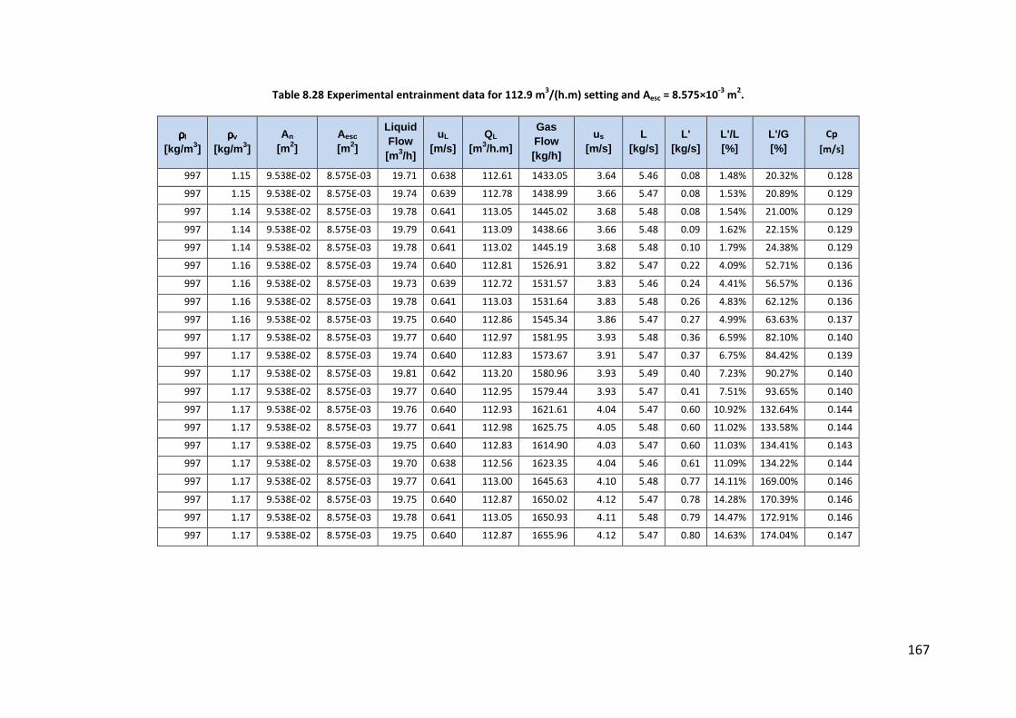
167


-3 m

2.

ρρρρl [kg/m 3]

ρρρρv [kg/m 3]

An [m 2]

Aesc [m 2]

Liquid Flow [m 3/h]

uL [m/s]

QL [m 3/h.m]

Gas Flow [kg/h]

us [m/s]

L [kg/s]

L' [kg/s]

L'/L [%]

L'/G [%]

Cp

[m/s]

997 1.15 9.538E-02 8.575E-03 19.71 0.638 112.61 1433.05 3.64 5.46 0.08 1.48% 20.32% 0.128

997 1.15 9.538E-02 8.575E-03 19.74 0.639 112.78 1438.99 3.66 5.47 0.08 1.53% 20.89% 0.129

997 1.14 9.538E-02 8.575E-03 19.78 0.641 113.05 1445.02 3.68 5.48 0.08 1.54% 21.00% 0.129

997 1.14 9.538E-02 8.575E-03 19.79 0.641 113.09 1438.66 3.66 5.48 0.09 1.62% 22.15% 0.129

997 1.14 9.538E-02 8.575E-03 19.78 0.641 113.02 1445.19 3.68 5.48 0.10 1.79% 24.38% 0.129

997 1.16 9.538E-02 8.575E-03 19.74 0.640 112.81 1526.91 3.82 5.47 0.22 4.09% 52.71% 0.136

997 1.16 9.538E-02 8.575E-03 19.73 0.639 112.72 1531.57 3.83 5.46 0.24 4.41% 56.57% 0.136

997 1.16 9.538E-02 8.575E-03 19.78 0.641 113.03 1531.64 3.83 5.48 0.26 4.83% 62.12% 0.136

997 1.16 9.538E-02 8.575E-03 19.75 0.640 112.86 1545.34 3.86 5.47 0.27 4.99% 63.63% 0.137

997 1.17 9.538E-02 8.575E-03 19.77 0.640 112.97 1581.95 3.93 5.48 0.36 6.59% 82.10% 0.140

997 1.17 9.538E-02 8.575E-03 19.74 0.640 112.83 1573.67 3.91 5.47 0.37 6.75% 84.42% 0.139

997 1.17 9.538E-02 8.575E-03 19.81 0.642 113.20 1580.96 3.93 5.49 0.40 7.23% 90.27% 0.140

997 1.17 9.538E-02 8.575E-03 19.77 0.640 112.95 1579.44 3.93 5.47 0.41 7.51% 93.65% 0.140

997 1.17 9.538E-02 8.575E-03 19.76 0.640 112.93 1621.61 4.04 5.47 0.60 10.92% 132.64% 0.144

997 1.17 9.538E-02 8.575E-03 19.77 0.641 112.98 1625.75 4.05 5.48 0.60 11.02% 133.58% 0.144

997 1.17 9.538E-02 8.575E-03 19.75 0.640 112.83 1614.90 4.03 5.47 0.60 11.03% 134.41% 0.143

997 1.17 9.538E-02 8.575E-03 19.70 0.638 112.56 1623.35 4.04 5.46 0.61 11.09% 134.22% 0.144

997 1.17 9.538E-02 8.575E-03 19.77 0.641 113.00 1645.63 4.10 5.48 0.77 14.11% 169.00% 0.146

997 1.17 9.538E-02 8.575E-03 19.75 0.640 112.87 1650.02 4.12 5.47 0.78 14.28% 170.39% 0.146

997 1.17 9.538E-02 8.575E-03 19.78 0.641 113.05 1650.93 4.11 5.48 0.79 14.47% 172.91% 0.146

997 1.17 9.538E-02 8.575E-03 19.75 0.640 112.87 1655.96 4.12 5.47 0.80 14.63% 174.04% 0.147

8.6 Data processing

Entrainment data was generated by logging the mass (in kilograms) in MV-202/4 (see Figure

3.8) every two seconds. During the sample the data was labelled (marked) so that MATLAB

(the mathematical software used for data processing) can find the groups of entrainment

data in the database (data was continuously logged during the experimental runs). A typical

sample will consist of 30 – 70 data points. MATLAB was then used to fit a linear model to the

data using linear regression, and data points that deviated with more than 2 standard

deviations were identified as outliers and subsequently removed. This ensured that all the

data was within the 95% confidence intervals. A final regression was then performed on the

data without the outliers and the gradient would be the entrained liquid flow rate measured

in kg/s.

Entrainment data for a given flow rate was then plotted as a function of the capacity factor

( ( )/p p g L gC u ρ ρ ρ= − ) and trendlines were fitted as shown in Figure 8.6 and Figure 8.7. To

verify that the trendlines are accurate the measured data was compared with the fitted data

in Figure 8.8. The solver function in Microsoft Excel was used to generate the entrainment

trends in Figure 4.6, Figure 4.7 and Figure 4.9 - Figure 4.13 which was within the measuring

range. None of the fitted experimental entrainment trends exceeded the measuring range

to insure interpolation and accuracy.

169

Figure 8.6 Fitting trendlines to entrainment data for each liquid flow rate [17.2 – 74.2 m3/(h.m)] as a

function of entrainment.

Figure 8.7 Fitting trendlines to entrainment data for each liquid flow rate [79.9 – 112.9 m3/(h.m)] as a

function of entrainment.

y = 22 668.5803x3 - 8 488.8056x2 + 1 063.5975x - 44.5160

R² = 0.9989

y = 435.787x2 - 107.560x + 6.680

R² = 0.996

y = 233.89x2 - 57.883x + 3.5933

R² = 0.9915

y = 211.73x2 - 54.923x + 3.5758

R² = 0.9921

y = 283.54x2 - 77.109x + 5.2669

R² = 0.9975

0%

5%

10%

15%

20%

25%

30%

35%

40%

45%

50%

0.120 0.130 0.140 0.150 0.160 0.170

L'/L

Cp [m/s]

QL = 17.2 m3/(h.m)

QL = 28.6 m3/(h.m)

QL = 40 m3/(h.m)

QL = 57.2 m3/(h.m)

QL = 74.2 m3/(h.m)

y = 3.3957E+09x1.2898E+01

R² = 9.9569E-01

y = 250.46x2 - 65.629x + 4.3141

R² = 0.9946

y = 332.47x2 - 84.192x + 5.3442

R² = 0.9964

0%

5%

10%

15%

20%

25%

0.120 0.130 0.140 0.150 0.160 0.170

L'/L

Cp [m/s]

QL = 79.9 m3/(h.m)

QL = 96.8 m3/(h.m)

QL = 112.9 m3/(h.m)

170

Figure 8.8 Verification of the fitted correlation for entrainment against the data.

y = x

0.00

0.05

0.10

0.15

0.20

0.25

0.30

0.35

0.40

0.45

0.50

0.00 0.05 0.10 0.15 0.20 0.25 0.30 0.35 0.40 0.45 0.50

L'/L

me

asu

red

L'/L Fitted

QL = 17.2 m3/(h.m)

QL = 28.6 m3/(h.m)

QL = 40 m3/(h.m)

QL = 57.2 m3/(h.m)

QL = 74.2 m3/(h.m)

QL = 79.9 m3/(h.m)

QL = 96.8 m3/(h.m)

QL = 112.9 m3/(h.m)

entrainment in an air/water system inside a sieve …

Documents