WORKING PAPER SERIES

Entrepreneurship and the Policy Environment

Yannis Georgellis and

Howard J. Wall

Working Paper 2002-019B http://research.stlouisfed.org/wp/2002/2002-019.pdf

September 2002 Revised March 2004

FEDERAL RESERVE BANK OF ST. LOUIS Research Division 411 Locust Street

St. Louis, MO 63102

______________________________________________________________________________________

The views expressed are those of the individual authors and do not necessarily reflect official positions of the Federal Reserve Bank of St. Louis, the Federal Reserve System, or the Board of Governors.

Federal Reserve Bank of St. Louis Working Papers are preliminary materials circulated to stimulate discussion and critical comment. References in publications to Federal Reserve Bank of St. Louis Working Papers (other than an acknowledgment that the writer has had access to unpublished material) should be cleared with the author or authors.

Photo courtesy of The Gateway Arch, St. Louis, MO. www.gatewayarch.com

1

ENTREPRENEURSHIP AND THE POLICY ENVIRONMENT

YANNIS GEORGELLIS and HOWARD J. WALL∗

December 2002, revised March 2004

This paper uses a spatial panel approach to examine the effect of the government-policyenvironment on the level of entrepreneurship. Specifically, we investigate whether marginalincome tax rates and bankruptcy exemptions influence rates of entrepreneurship. Whereasprevious work in the literature finds that both policies are positively related to entrepreneurship,we find non-monotonic relationships: a U-shaped relationship between marginal tax rates andentrepreneurship and an S-shaped relationship between bankruptcy exemptions andentrepreneurship. (JEL J23, R12)

I. INTRODUCTION

Entrepreneurship is thought to be an important factor in spawning innovation,

employment, and economic growth. Because the benefits flowing from entrepreneurship are not

necessarily captured by the entrepreneurs themselves, but can be realized more generally, the

case is often made that the level of entrepreneurship is below its social optimum and deserves

some attention from policymakers. Despite the recognized importance of entrepreneurship,

however, there has been relatively little empirical analysis of the role played by the government-

policy environment.

Previous research on self-employment and entrepreneurship has examined the roles of

various demographic, human capital, and financial considerations in the decision to become an

entrepreneur. Typically, studies have indicated the importance of (i) the earnings differential

∗ We would like to acknowledge the comments and suggestions of two anonymous referees, Kate Antonovics,

Mark Partridge, Mike Dueker, and seminar participants at Southern Illinois University at Carbondale and the AnnualConference of the Western Economic Association International, Seattle, June 29-July 3, 2002. We would also liketo acknowledge the research assistance of Paige Skiba. The views expressed are those of the authors and do notnecessarily represent official positions of the Federal Reserve Bank of St. Louis or the Federal Reserve System.

Y. Georgellis: Senior Lecturer, Department of Economics and Finance, Brunel University, Uxbridge, UB8 3PH, UK.Phone 01895 203174, Fax 01895 203384, E-mail yannis.georgellis@brunel.ac.uk

H. Wall: Research Officer, Federal Reserve Bank of St. Louis, 411 Locust Street, St. Louis, MO 63166. Phone 314-444-8533, Fax 314-444-8731, E-mail wall@stls.frb.org

2

between entrepreneurship and paid employment (Rees and Shah, 1986; Gill, 1988; Hamilton,

2000); (ii) liquidity constraints (Evans and Jovanovic, 1989; Evans and Leighton, 1989, Holtz-

Eakin et al., 1994 and 1994b; Black and Strahan, 2002); (iii) satisfaction differentials (Taylor,

1996; Blanchflower and Oswald 1998; Blanchflower, 2000); (iv) macroeconomic conditions

(Taylor, 1996; Parker, 1996; Cowling and Mitchell, 1997); and (v) intergenerational human

capital transfers (Dunn and Holtz-Eakin, 2000; Hout and Rosen, 2000).1

Empirical studies that have considered the effects of the policy environment on

entrepreneurship have focused on personal income tax rates, with the expectation that higher tax

rates should suppress entrepreneurship. Nearly all studies, however, have found a positive

relationship, whether it is between tax rates and aggregate rates of entrepreneurship (Long,

1982a; Evans and Leighton, 1989; Blau, 1987; Parker, 1996; Robson, 1998; and Bruce and

Mohsin, 2003) or between tax rates and the individual-level probability of entrepreneurship

(Long, 1982b; Scheutze, 2000; Fan and White, 2003). This divergence between expectations

and results is usually attributed to the perception that, because of the nature of a tax system that

relies on self-reporting, being an entrepreneur allows for relatively greater opportunities for tax

avoidance.2 Cullen and Gordon (2002), however, argue that, because entrepreneurs have the

option of whether or not to incorporate their business, and because personal income tax rates are

higher than corporate ones, the tax system provides a net subsidy to risk-taking. This is because

an entrepreneur facing losses would prefer to face personal income tax rates so that the deduction

of the losses against other income would have greater tax-reducing value. All else equal, an

1. Le (1999) provides a fairly comprehensive survey of the empirical literature.2. Robson and Wren (1999) is an exception that finds a negative relationship between tax rates and

entrepreneurship. They also have a theoretical model of tax avoidance and the entrepreneurial decision.

3

increase in personal income tax rates make this option more valuable, thereby increasing the

likelihood that someone would choose to become an entrepreneur.

Other studies have begun to look at the question of taxes and entrepreneurship using

more-complicated indicators of the tax system. Robson and Wren (1999) separate the effects of

average and marginal tax rates, suggesting that the former represents the incentive for tax

avoidance while the latter represents the disincentive effect.3 Bruce (2000) looks at the

differential tax treatment of self-employment and wage-and-salary earnings, finding that

marginal and average tax rates on self-employment earnings are negatively related to the

probability of becoming self-employed. Gentry and Hubbard (2000) find that the more

progressive a tax system is, the less likely it is that an individual will enter self-employment.

Bruce, Deskins, and Mohsin (2003) look at state-level differences in a variety of tax policies,

including rates of sales taxes and personal and corporate income taxes, along with whether states

allow combined reporting and limited liability corporations.

A recently opened line of inquiry into the effects of the policy environment on

entrepreneurship has raised the question of whether or not bankruptcy laws affect the number of

entrepreneurs (Berkowitz and White, 2004; Fan and White, 2003; White, 2001). Briefly, U.S.

bankruptcy laws allow individuals filing for personal bankruptcy to exempt some of their assets

and income from distribution to their creditors. The exemptions, which differ a great deal across

states, can include some or all of the value of a person’s home (the homestead exemption),

pension holdings, and an assortment of other assets.4

3. Their theoretical model separates the tax effects into pure marginal and pure average tax changes, roughly

analogous to substitution and income effects. Unfortunately, the tax rates they use in their empirical analysis aresimply the average and marginal tax rates, each of which has income and substitution effects.

4. For detailed discussions of U.S. personal bankruptcy laws and the incentives they create, see White (1998),Fay, Hurst, and White (2002), Gropp, Scholz, and White (1997), and Dye (1986).

4

The direct effect of these exemptions is to provide a sort of wealth insurance in the event

that an entrepreneurial venture fails. Thus, by this wealth-insurance effect, higher exemption

levels should lead to more entrepreneurs. Less direct than the wealth-insurance effect is a credit-

access effect, which works in the opposite direction. It arises because banks and other credit

providers adjust their actions in response to changes in bankruptcy exemptions. As a result, the

higher the exemption level, the less credit will be available at a given interest rate.5 These two

opposing effects of bankruptcy exemptions on entrepreneurship mean that the sign of the total

effect is ambiguous in general. However, Fan and White (2003) find that the wealth-insurance

effect dominates the credit-access effect for all levels of the exemption. In fact, they find that

homeowners in states with an unlimited homestead exemption are 35 percent more likely to be

self-employed than equivalent homeowners in states with low exemption levels.

In an attempt to resolve the results on the effects of taxes and to enhance the modeling of

bankruptcy exemptions, this paper takes a different approach to estimating the effects of

government policies on entrepreneurship. Specifically, following Georgellis and Wall (2000a),

we create a state-level panel dataset that pools observations over space and time.6 This allows us

to look at the effects of changes in policies over time while exploiting the large differences

across states in levels of entrepreneurship, bankruptcy exemptions, and tax rates. The

advantages of this approach over aggregate time-series studies ― which have only one

observation per time period ― are that we can include a large number of control variables, use

more-general specifications of policy variables, and control for trends more effectively. Another

advantage, which we outline in greater detail below, is that it allows us to create a continuous

5. Berkowitz and White (2002) show how small, unincorporated businesses face lower credit access and

higher interest rates in states with higher exemption levels.6. See also Wall (2004); Bruce, Deskins, and Mohsin (2003); and Black and Strahan (2002).

5

variable for the homestead exemption, rather than having to group different exemption levels

together into dummy variables, as is necessary when using individual-level panels.

Using the spatial-panel approach, we find a U-shaped relationship between marginal tax

rates and entrepreneurship. At low tax rates the relationship is negative, and at high rates it is

positive. Also, we find an S-shaped relationship between the homestead exemption and

entrepreneurship. Specifically, an increase in the homestead exemption from very low or very

high levels acts to reduce the number of entrepreneurs, while an increase in the middle range acts

to increase the number of entrepreneurs.

II. SPATIAL AND TEMPORAL TRENDS IN U.S. ENTREPRENEURSHIP

We define the rate of entrepreneurship as the proportion of the working-age population

that is classified as nonfarm proprietors. In common with most of the literature, we exclude farm

proprietors on the grounds that the decision to become a farm proprietor depends on different

factors than the decision to become a nonfarm proprietor, and because farmers operate under

different bankruptcy laws than do other proprietors.

Proprietors’ employment is the number of people who are employed in their own

business, regardless of whether that business is incorporated. Various other measures of

entrepreneurship have been used in the literature, such as the non-farm self-employed, which

excludes farmers and the incorporated.7 The rate of entrepreneurship is usually calculated with

the labor force or total employment in the denominator. We prefer to use the working-age

population because, unlike the size of the labor force or the number employed, it is not likely to

move with the number of entrepreneurs as people move between employment states. This

7. Bruce and Holtz-Eakin (2001) examine a variety of measures and conclude that it makes little difference

which one is used.

6

distinction also recognizes the fact that entrepreneurs are drawn from the entire working-age

population, not just those currently employed or in the labor force.

Figures 1a and 1b illustrate the cross-state differences in the levels and growth of

entrepreneurship during our sample period, 1991-98. In general, states in the western half of the

country had the highest levels of entrepreneurship. The eastern part of the country contained all

of the regions with the lowest rates of entrepreneurship: the Great Lakes, the Upper South, and

the Deep South. In the East, only New England states were in the top two quartiles of

entrepreneurship. As Figure 1b shows, all states saw increases in their rates of entrepreneurship

between 1991 and 1998, and there was some convergence. Southern states, New York, and the

lagging western states had the highest growth in entrepreneurship, while much of the West saw

relatively little growth.

III. EMPIRICAL MODEL

Assume that each person has the option of being an employee of someone else, becoming

an entrepreneur, or not working. The utility outcomes of these options are uncertain and depend

on prevailing market conditions and the person’s abilities and preferences in each of the

activities. Define the mean person as that member of a state or national population who

possesses the mix of characteristics and skills expected of a randomly selected person. Denote

the utility that the country’s mean person would attain as: an entrepreneur in state i as eiU , an

employee as miU , and not working as n

iU . For the country’s mean person, the utility levels in

these activities differ across states because of differences in industrial mix, business conditions,

government policies, and amenities.

7

For state i’s mean person, the difference in utility between entrepreneurship and

employment is ,imi

ei UU δ+− where δi differentiates the mean person in the state from the mean

person in the country as a whole. δi differs across states because of spatial differences in

education levels, age, entrepreneurial human capital, and other individual characteristics, some

of which are unobservable or unmeasurable. Similarly, for state i’s mean person, the difference

in utility between entrepreneurship and not working is ,ini

ei UU λ+− where iλ differentiates

the mean person in the state from the mean person in the country as a whole.

Define a random variable eij such that 1=ije if person j in state i is an entrepreneur and

0=ije otherwise. If person j were selected randomly from state i, the probability that he would

be an entrepreneur is the probability that entrepreneurship provides a higher level of utility to

state i’s mean person than do the alternatives:

(1) ].0 ,0Pr[]1Pr[ >λ+−>δ+−== ini

eii

mi

eiij UUUUe

Summing (1) across the Ni people in i and dividing by the population, Ni,

(2) ), ,(]1Pr[1

1i

ni

eii

mi

ei

N

jij

ii UUUUFe

NE

iλ+−δ+−==≡ ∑

=

where 0 and 21 >FF . Assuming a large enough population, Ei is the rate of entrepreneurship in

state i.

According to equation (2), a state’s rate of entrepreneurship increases along with the

relative utility that entrepreneurship provides for the state’s mean person. This differs across

states because (i) state labor forces differ in their relative skills and preferences for

entrepreneurship (i.e., δ i and iλ differ across states) and (ii), controlling for individual

8

characteristics, the relative suitability for entrepreneurship differs across states (i.e., mi

ei UU −

and ni

ei UU − differ by state).

Using t to denote the time period, assume that (2) can be estimated with the following

regression equation:

(3) .ittiitE ε+′+++τ+α= ititit GγZθ'Xβ'

In equation (3), iα is a state-specific component that is constant over time and tτ is a year-

specific component that is common to all states. The vectors Zit and Xit measure, respectively,

business conditions and average demographic characteristics in state i in year t. Government

policy variables are included in the vector Git, and itε is the error term.

IV. DATA

The demographic variables included in Xit capture the spatial and temporal differences in

age, gender, and racial compositions of state populations. As outlined in Georgellis and Wall

(2000b), rates of self-employment differ a great deal across these categories. We therefore

include age variables that measure differences in population shares of broad age categories.

Also, because men are nearly twice as likely as women to be self-employed, we include the

female share of a state’s population. Finally, Xit includes the black, Native American, Asian and

Pacific Islander, and Hispanic population shares. Large variations in self-employment across

these groups might explain state-level differences in entrepreneurship. For example, the self-

employment rate for blacks is only about one-third of that for whites and Asians.

Here and in the previous section we discuss these variables in terms of the supply of

potential entrepreneurs. However, one should be careful about the interpretation of the estimated

9

coefficients because these demographic groups might also differ in their demand for the products

that are more likely to be produced by entrepreneurs. For example, as Georgellis and Wall

(2000b) report, over 10 percent of self-employed women in 1997 were in the child-care business,

while virtually no men were. This indicates that a state with a higher-than-average female

population share might have a higher-than-average supply of child-care providers. On the other

hand, such a state also has a higher-than-average number of women demanding child-care

services.

The vector of business conditions, Zit, includes measures of a state’s economy that affect

the profitability of entrepreneurship. These include the state’s unemployment rate, per capita

real income, per capita real wealth (as proxied by dividends, interest, and rent), relative

proprietor’s wage, and industry employment shares. As with our demographic variables, the

interpretation of the roles of these variables is not entirely clear because each can simultaneously

indicate the demand for entrepreneurs’ services and the supply of entrepreneurs. For example,

while we include the unemployment rate as a measure of the health of a state’s economy, Parker

(1996), among others, includes it as an indicator of the number of people with limited

opportunities for wage-and-salary employment who might be pushed into self-employment.

As Georgellis and Wall (2000a) demonstrate, the specification of our control variables ―

the elements of Xit and Zit ― is potentially important. They show, for example, that the

relationship between the rates of self-employment and unemployment in Britain is hill-shaped.

Indeed, the best fit in the present context would allow for nonlinear relationships. Nonetheless,

our present purpose is to estimate the effects of taxes and the homestead exemption, and a simple

linear specification for the control variables makes little difference in this regard. Therefore, for

parsimony, we use a linear specification for these control variables.

10

Presently, the variables of most interest are those measuring marginal tax rates and the

homestead exemption. For the former, we use the maximum marginal tax rates (state plus

federal) as generated by the NBER’s TAXSIM model (see Table 1 for the state maximum

marginal tax rates in 1990 and 1997, the first and last years of data used in our study). Of the tax

rate measures used in the literature, this one best fits our needs. For one, it is the measure used

in the paper most comparable to ours, Fan and White (2003). But, more importantly, it is

exogenous, unlike the average marginal tax rate also generated by TAXSIM. While very few

people will actually face the maximum marginal tax rate, there should be a very strong

correlation between the marginal tax rates that the average person faces and the maximum rate.

We constructed our homestead exemption variable to take into account several state-level

differences in bankruptcy law. First, as noted above and as summarized by Table 1, there are

large differences in the exemption level across states: In 1997, five states did not allow any

homestead exemption, while seven had an unlimited exemption. Also, some states allow for the

federal exemption to be substituted at the filer’s discretion, and some states allow married filers

to double the exemption level. Because our variable is meant to capture the exemption that the

average person in a state might face, we also take into account differences in the average house

prices and the likelihood that a filer owns rather than rents.

Our homestead exemption variable starts by taking the state exemption level or, if the

state allows the federal option, the maximum of the state and federal exemption levels. If this is

greater than the average house price in the state, we use the average house price instead, which is

a more accurate representation of the exemption that the average person would get. We then

multiplied this by the state’s homeownership rate and, if the state allows married householders to

double the exemption, we also multiply it by one plus the state’s share of households in which

11

both spouses reside together. The result of this divided by the average house price yields our

homestead exemption rate.

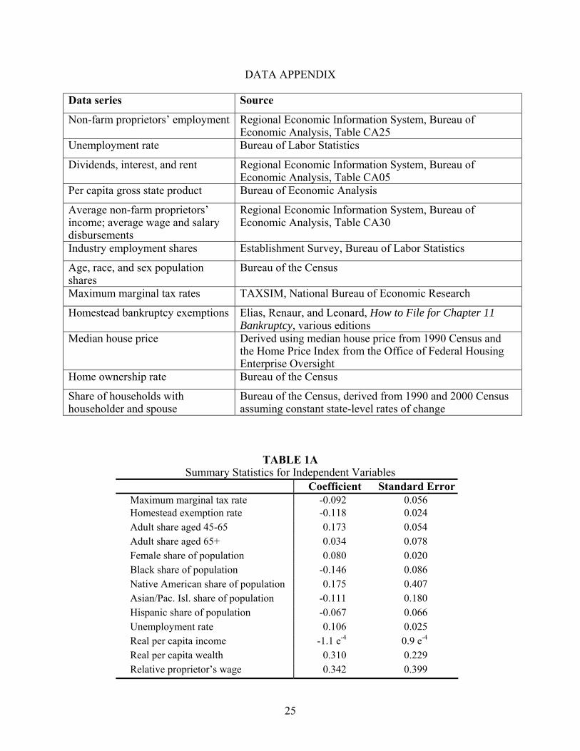
Note that the sources for all of the data used to construct our variables are given in the

data appendix, as are the summary statistics for all of the independent variables described above.

We should also note that our two most important dependent variables — the homestead

exemption rate and the maximum marginal tax rate — are statistically independent, as indicated

by their correlation coefficient of -0.01.

As we mention above, one of the main benefits of our spatial panel approach is that the

relative abundance of observations means that we can easily allow for non-linearities. This is

important because, for each of our government policy variables, there are opposing effects,

meaning that the relationships might be non-monotonic. This is easiest to see with tax rates, for

which the standard negative labor-effort effect is countered by the positive tax-avoidance effect.

Assuming a non-trivial cost to being caught avoiding taxes, at low tax rates the incentive to

avoid taxes will not be terribly strong because the net expected benefits are not very high.

Conversely, under very high tax rates, the benefit of avoiding taxes is much higher.

Our choice of functional form for the tax and homestead exemption variables is crucial to

our results. Theory gives us no guidance on the appropriate specification; so, to be as general as

reasonably possible, we began with a cubic form for both variables. This specification fits the

homestead exemption rate well, yielding statistically significant coefficients for all three terms.

However, because the coefficients on all three terms for the tax variable were not statistically

different from zero, we re-estimated using a quadratic specification, which yielded two

statistically significant coefficients. Thus, our baseline model, which we report and discuss in

12

detail below, uses a quadratic tax variable and a cubic homestead exemption variable. In the

section following our discussion of the baseline results, we discuss alternative specifications.

V. EMPIRICAL RESULTS

Our dependent variable is the rate of entrepreneurship, as defined above, for 1991-1998,

and our independent variables are all lagged by one year. To allow for the most general error

structure given our data constraints, we estimate (3) using feasible generalized least squares

(FGLS). This allows for state-specific heteroskedastic errors, although, because of a relatively

short panel, we still need to assume that errors are uncorrelated across states.8 We also allow for

each state’s errors to follow their own AR(1) process.

Table 2 summarizes our results. As discussed above, we attach little importance to the

coefficients on our demographic and business conditions variables, but simply note that omitting

them would have a statistically significant effect on the results. More importantly, our

estimation indicated that the marginal tax rate and the homestead exemption rate are both related

non-monotonically to the rate of entrepreneurship.

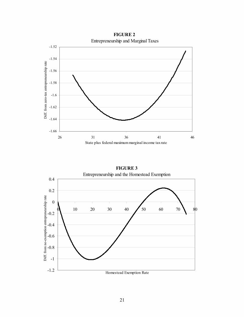
Our estimates of the effects of marginal tax rates on entrepreneurship indicate that at tax

rates at the low end of our observed rates ― 28 to 35 percent ― an increase in the tax rate will

reduce the number of entrepreneurs (see Figure 2). Beyond this range, higher marginal taxes

will increase the number of entrepreneurs indirectly as, presumably, the tax-avoidance incentives

become large enough to begin outweighing the possible penalties.

The cubic relationship between the homestead exemption rate and entrepreneurship is

illustrated by Figure 3. At very low and very high exemption rates ― between 0 and 20 percent

8. A useful rule of thumb is that there are twice as many time periods as cross-sectional units (Beck and Katz,

1995).

13

and above 60 percent ― an increase in the homestead exemption leads to a decrease in the rate

of entrepreneurship, suggesting that the credit-access effect dominates. At the mid-range of

exemption rates ― between 20 and 60 percent ― an increase in the homestead exemption rate

leads to an increase in the rate of entrepreneurship, suggesting that the wealth-insurance effect

dominates. Note, though, that only rates between 50 and 72 percent lead to a higher rate of

entrepreneurship than there would be with no homestead exemption at all.

The year dummies are also interesting and suggest an underlying trend in

entrepreneurship not captured by demographics, business conditions, or government policies.

The estimated coefficient on the 1998 dummy indicates that state rates of entrepreneurship

would have risen, on average, by 1.2 percentage points from 1991 to 1998 if all of the variables

we include in our estimation remained at their initial levels.

Figure 4 plots the estimated fixed effects across the states, illustrating the extent to which

differences in entrepreneurship are determined by differences in the variables included in our

regression. Most noticeably, comparing Figures 1a and 4, we see that not all states with low

levels of entrepreneurship also have low estimated fixed effects. In particular, states in the Great

Lakes, Upper South, and Deep South regions have low levels of entrepreneurship, typically

falling in the lowest quartile. However, the fixed effects for the Deep South states are not in the

lowest quartile, while those for the Great Lakes and Upper South states are. This indicates that

the relatively low levels of entrepreneurship in the Deep South are due to relatively inhospitable

business conditions, demographic factors, or government policies. On the other hand, the low

levels of entrepreneurship in the Great Lakes and Upper South are attributable to fixed factors,

which Georgellis and Wall (2000a) suggest might include cultural, historical, or sociological

factors that suppress entrepreneurship. At the other extreme are states in New England and the

14

West, which have high levels of entrepreneurship and high estimated fixed effects. This suggests

that one of the reasons for the high levels of entrepreneurship are that these states contain the

cultural, historical, and sociological makeup to pursue and succeed in entrepreneurship.

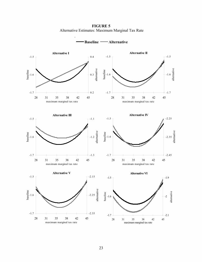
VI. ALTERNATIVE ESTIMATES

Our baseline model uses specific functional forms for the policy variables and

generalized least-squares estimation to allow for state-specific autocorrelation and cross-

sectionally uncorrelated heteroskedasticity. To check the consequence of these choices on our

estimation of the effects of our policy variables, we present the results of six alternatives.9 These

alternative results, which either use a different specification of the policy variables or place

stronger restrictions on the error terms, are reported in Table 3 and illustrated by Figures 5 and 6.

Alternative I restricts the coefficients on the squared and cubed terms of the policy

variables to zero. Estimation under these restrictions yields a positive and statistically significant

effect for the marginal tax rate on entrepreneurship and a negative but statistically insignificant

effect for the homestead exemption rate. Alternative II restricts the coefficient on the cubed term

of the homestead exemption rate to zero while using the same quadratic functional form for the

marginal tax rate as in the baseline model. The estimated relationship between the maximum

marginal tax rate and entrepreneurship under this restriction differs very little from the baseline

results. On the other hand, as previously stated, the estimated coefficients on the homestead

exemption rate are both statistically no different from zero. The results from these two

alternative specifications indicate that the choices we have made about the specification of the

policy variables are important for our conclusions. Likelihood ratio tests reject the null

9. Wall (2004) demonstrates how not allowing for autocorrelation and heteroskedasticity, in particular, has

severe consequences for the state-level panel of entrepreneurship in Black and Strahan (2002).

15

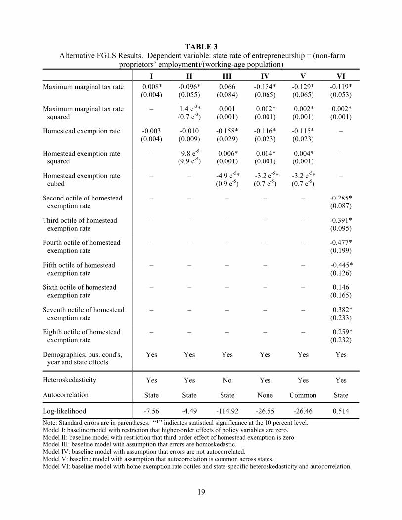
hypotheses that the restrictions that these alternatives place on the higher-order terms do not have

a statistically significant effect on the estimation. Therefore, the least-restrictive baseline model

is preferred statistically to the two alternatives.

Three other alternatives place stronger restrictions on the error terms than does the

baseline model: In alternative III they are assumed to be homoskedastic, in alternative IV they

are not autocorrelated, and in alternative V their autocorrelation is common across states. As

Figure 5 illustrates, none of these restrictions has an effect on the estimated U shape for the

relationship between marginal tax rates and the rate of entrepreneurship, although the

coefficients in alternative III are not statistically significant. The important differences are that

the estimated relationship is flatter with alternative III and steeper with alternatives IV and V.

For the relationship between the homestead exemption rate and the rate of

entrepreneurship, only the estimates from alternative III differ in any non-trivial way. All three

alternatives yield an S-shaped relationship, although the estimated relationship is everywhere

steeper with alternative III than with the baseline model. Another important difference is that

alternative III suggests that all homestead exemption rates above 42 percent will yield more

entrepreneurship than would a zero exemption, whereas the baseline model suggests that this is

true only for homestead exemption rates between 50 and 72 percent.

Alternative VI replaces the continuous homestead exemption variables with dummy

variables for discrete ranges of the homestead exemption rate. Because this removes any general

assumption regarding functional form, it allows us to verify the general shape of the cubic

relationship of our baseline model. We split the observed homestead exemption rates into

octiles, each with 50 observations, and estimate the model with the first octile omitted to avoid

perfect collinearity. As summarized by Table 3, for all but one of the octiles of the homestead

16

exemption rate, the rate of entrepreneurship is statistically different from what it would be under

the first octile. Further, as illustrated by Figure 6, these results confirm the general S-shape to

the relationship between the homestead exemption rate and the rate of entrepreneurship. Note

also that this specification has little effect on the estimated relationship between the rate of

entrepreneurship and the maximum marginal tax rate.

VII. CONCLUDING REMARKS

This paper uses the spatial panel approach of Georgellis and Wall (2000a) to estimate the

effects of personal income tax rates and bankruptcy exemptions on entrepreneurship. Using data

for all 50 states of the United States for 1991-1998, we find non-homothetic relationships.

Specifically, at low initial tax levels, an increase in marginal tax rates reduces the number of

entrepreneurs, although at higher initial tax levels it will do the opposite. We also find that at

very low and very high initial levels an increase in the homestead exemption will reduce the

number of entrepreneurs. In the mid-range of homestead exemption rates there is a positive

relationship between the exemption level and entrepreneurship. Further, only for relatively high

homestead exemption rates will the level of entrepreneurship be higher than if there were no

homestead exemption at all.

17

TABLE 1 State Homestead Exemptions and Maximum Marginal Tax Rates

Maximum Marginal Tax Rates Homestead ExemptionsState 1990 1997 1990 1997Alabama 3.65 3.12 $5,000 $5,000Alaska 0 0 54,000 54,000Arizona 6.51 4.8 100,000 100,000Arkansas 7 7 no limit no limitCalifornia 9.3 9.78 7,500 15,000Colorado 4.76 5.36 20,000 30,000Connecticut 0 4.5 0 75,000Delaware 7.7 6.9 0 0Florida 0 0 no limit no limitGeorgia 5.66 5.83 5,000 5,000Hawaii 9 9 30,000 30,000Idaho 8.2 8.2 30,000 50,000Illinois 3 3 7,500 7,500Indiana 3.4 3.4 7,500 7,500Iowa 7.39 6.36 no limit no limitKansas 5.15 6.45 no limit no limitKentucky 4.39 6 5,000 5,000Louisiana 4.14 3.75 15,000 15,000Maine 8.5 8.5 7,500 12,500Maryland 5 6 0 0Massachusetts 5.95 5.95 100,000 100,000Michigan 4.6 4.4 3,500 3,500Minnesota 8 8.86 no limit 200,000Mississippi 4.75 4.85 30,000 75,000Missouri 4.39 6 8,000 8,000Montana 8.59 6.83 40,000 40,000Nebraska 6.4 7 10,000 10,000Nevada 0 0 90,000 125,000New Hampshire 0 0 5,000 30,000New Jersey 3.5 6.37 0 0New Mexico 7.83 8.4 20,000 30,000New York 7.88 6.85 10,000 10,000North Carolina 7 8.08 7,500 10,000North Dakota 3.77 5.25 80,000 80,000Ohio 6.9 7.2 5,000 5,000Oklahoma 6.72 6.05 no limit no limitOregon 8.12 9 15,000 25,000Pennsylvania 2.1 2.8 0 0Rhode Island 6.04 9.66 0 0South Carolina 7 7.3 5,000 5,000South Dakota 0 0 no limit no limitTennessee 0 0 5,000 5,000Texas 0 0 no limit no limitUtah 6.26 5.72 8,000 8,000Vermont 6.54 8.85 30,000 30,000Virginia 5.75 5.75 5,000 5,000Washington 0 0 30,000 30,000West Virginia 6.5 6.5 7,500 15,000Wisconsin 6.93 6.93 40,000 40,000Wyoming 0 0 10,000 10,000Federal 7,500 15,000

18

TABLE 2Baseline FGLS Results. Dependent variable: state rate of entrepreneurship = (non-farm

proprietors’ employment)/(working-age population)Coefficient Standard Error t-statistic

PoliciesMaximum marginal tax rate -0.092 0.056 -1.66Maximum marginal tax rate squared 1.3 e-3 0.7 e-3 1.75Homestead exemption rate -0.118 0.024 -4.93Homestead exemption rate squared 0.004 0.001 4.77Homestead exemption rate cubed -3.3 e-5 0.7 e-5 -4.69

DemographicsAdult share aged 45-65 0.173 0.054 3.22Adult share aged 65+ 0.034 0.078 0.44Female share of population 0.080 0.020 4.06Black share of population -0.146 0.086 -1.70Native American share of population 0.175 0.407 0.43Asian/Pac. Isl. share of population -0.111 0.180 -0.62Hispanic share of population -0.067 0.066 -1.01

Business conditionsUnemployment rate 0.106 0.025 4.26Real per capita income -1.1 e-4 0.9 e-4 -1.23Real per capita wealth 0.310 0.229 1.35Relative proprietor’s wage 0.342 0.399 0.86Industry shares Yes ― ―

Year dummies1992 -0.221 0.055 -4.011993 -0.106 0.090 -1.181994 0.207 0.119 1.731995 0.606 0.152 3.981996 1.038 0.183 5.671997 1.153 0.219 5.251998 1.224 0.255 4.81

State fixed effects Yes ― ―Constant -22.442 119.659 -0.19Log-likelihood -6.291Number of observations 400Estimated covariances 50Estimated autocorrelations 50Note: The estimation corrects for state-specific heteroskedasticity and autocorrelation. Omittedreference variables are: adult share aged 18-44, white share of population, government share ofemployment, and 1991.

19

TABLE 3 Alternative FGLS Results. Dependent variable: state rate of entrepreneurship = (non-farm

proprietors’ employment)/(working-age population)I II III IV V VI

Maximum marginal tax rate 0.008*(0.004)

-0.096*(0.055)

0.066(0.084)

-0.134*(0.065)

-0.129*(0.065)

-0.119*(0.053)

Maximum marginal tax ratesquared

– 1.4 e-3*(0.7 e-3)

0.001(0.001)

0.002*(0.001)

0.002*(0.001)

0.002*(0.001)

Homestead exemption rate -0.003(0.004)

-0.010(0.009)

-0.158*(0.029)

-0.116*(0.023)

-0.115*(0.023)

–

Homestead exemption ratesquared

– 9.8 e-5

(9.9 e-5) 0.006*(0.001)

0.004*(0.001)

0.004*(0.001)

–

Homestead exemption ratecubed

– – -4.9 e-5*(0.9 e-5)

-3.2 e-5*(0.7 e-5)

-3.2 e-5*(0.7 e-5)

–

Second octile of homesteadexemption rate

– – – – – -0.285*(0.087)

Third octile of homesteadexemption rate

– – – – – -0.391*(0.095)

Fourth octile of homesteadexemption rate

– – – – – -0.477*(0.199)

Fifth octile of homesteadexemption rate

– – – – – -0.445*(0.126)

Sixth octile of homesteadexemption rate

– – – – – 0.146(0.165)

Seventh octile of homesteadexemption rate

– – – – – 0.382*(0.233)

Eighth octile of homesteadexemption rate

– – – – – 0.259*(0.232)

Demographics, bus. cond's,year and state effects

Yes Yes Yes Yes Yes Yes

Heteroskedasticity Yes Yes No Yes Yes Yes

Autocorrelation State State State None Common State

Log-likelihood -7.56 -4.49 -114.92 -26.55 -26.46 0.514Note: Standard errors are in parentheses. “*” indicates statistical significance at the 10 percent level.Model I: baseline model with restriction that higher-order effects of policy variables are zero.Model II: baseline model with restriction that third-order effect of homestead exemption is zero.Model III: baseline model with assumption that errors are homoskedastic.Model IV: baseline model with assumption that errors are not autocorrelated.Model V: baseline model with assumption that autocorrelation is common across states.Model VI: baseline model with home exemption rate octiles and state-specific heteroskedasticity and autocorrelation.

20

FIGURE 1aAverage Rates of Entrepreneurship, 1991-98

16.6 to 20 .2 (11)14.5 to 16 .6 (13)12.2 to 14 .5 (12)10.5 to 12 .2 (14)

FIGURE 1b Percentage Change in Rates of Entrepreneurship, 1991-98

14.2 to 22.4 (12)11.9 to 14.2 (11)

9.1 to 11.9 (13)3.8 to 9.1 (14)

21

FIGURE 2 Entrepreneurship and Marginal Taxes

-1.66

-1.64

-1.62

-1.6

-1.58

-1.56

-1.54

-1.52

26 31 36 41 46State plus federal maximum marginal income tax rate

Diff

. fro

m z

ero-

tax

entre

pren

eurs

hip

rate

FIGURE 3Entrepreneurship and the Homestead Exemption

-1.2

-1

-0.8

-0.6

-0.4

-0.2

0

0.2

0.4

0 10 20 30 40 50 60 70 80

Homestead Exemption Rate

Diff

. fro

m n

o-ex

empt

ion

entre

pren

eurs

hip

rate

22

FIGURE 4Estimated State Fixed Effects

-2.4 to 2.7 (11)-4.1 to -2.4 (13)-5.4 to -4.1 (12)-9.5 to -5.4 (14)

23

FIGURE 5 Alternative Estimates: Maximum Marginal Tax Rate

-1.7

-1.6

-1.5

28 31 35 38 42 45maximum marginal tax rate

base

line

0.2

0.3

0.4

alte

rnat

ive

Alternative I

-1.7

-1.6

-1.5

28 31 35 38 42 45maximum marginal tax rate

base

line

-1.7

-1.6

-1.5

alte

rnat

ive

Alternative II

-1.7

-1.6

-1.5

28 31 35 38 42 45maximum marginal tax rate

base

line

-1.3

-1.2

-1.1

alte

rnat

ive

Alternative III

-1.7

-1.6

-1.5

28 31 35 38 42 45maximum marginal tax rate

base

line

-2.45

-2.35

-2.25

alte

rnat

ive

Alternative IV

-1.7

-1.6

-1.5

28 31 35 38 42 45maximum marginal tax rate

base

line

-2.35

-2.25

-2.15

alte

rnat

ive

Alternative V Alternative VI

-1.7

-1.6

-1.5

28 31 35 38 42 45maximum marginal tax rate

base

line

-2.1

-2

-1.9

alte

rnat

ive

Baseline Alternative

24

FIGURE 6 Alternative Estimates: Homestead Exemption Rate

Alternative I

-1.4

-1.0

-0.6

-0.2

0.2

0.6

1.0

0 10 20 30 40 50 60 70

Homestead exemption rate

Alternative II

-1.4

-1.0

-0.6

-0.2

0.2

0.6

1.0

0 10 20 30 40 50 60 70

Homestead exemption rate

Alternative III

-1.4

-1.0

-0.6

-0.2

0.2

0.6

1.0

0 10 20 30 40 50 60 70

Homestead exemption rate

Alternative IV

-1.4

-1.0

-0.6

-0.2

0.2

0.6

1.0

0 10 20 30 40 50 60 70

Homestead exemption rate

Alternative V

-1.4

-1.0

-0.6

-0.2

0.2

0.6

1.0

0 10 20 30 40 50 60 70

Homestead exemption rate

Alternative VI

-1.4

-1.0

-0.6

-0.2

0.2

0.6

1.0

0 10 20 30 40 50 60 70

Homestead exemption rate

Baseline Alternative

25

DATA APPENDIX

Data series Source

Non-farm proprietors’ employment Regional Economic Information System, Bureau ofEconomic Analysis, Table CA25

Unemployment rate Bureau of Labor Statistics

Dividends, interest, and rent Regional Economic Information System, Bureau ofEconomic Analysis, Table CA05

Per capita gross state product Bureau of Economic Analysis

Average non-farm proprietors’income; average wage and salarydisbursements

Regional Economic Information System, Bureau ofEconomic Analysis, Table CA30

Industry employment shares Establishment Survey, Bureau of Labor Statistics

Age, race, and sex populationshares

Bureau of the Census

Maximum marginal tax rates TAXSIM, National Bureau of Economic Research

Homestead bankruptcy exemptions Elias, Renaur, and Leonard, How to File for Chapter 11Bankruptcy, various editions

Median house price Derived using median house price from 1990 Census andthe Home Price Index from the Office of Federal HousingEnterprise Oversight

Home ownership rate Bureau of the Census

Share of households withhouseholder and spouse

Bureau of the Census, derived from 1990 and 2000 Censusassuming constant state-level rates of change

TABLE 1ASummary Statistics for Independent Variables

Coefficient Standard ErrorMaximum marginal tax rate -0.092 0.056Homestead exemption rate -0.118 0.024Adult share aged 45-65 0.173 0.054Adult share aged 65+ 0.034 0.078Female share of population 0.080 0.020Black share of population -0.146 0.086Native American share of population 0.175 0.407Asian/Pac. Isl. share of population -0.111 0.180Hispanic share of population -0.067 0.066Unemployment rate 0.106 0.025Real per capita income -1.1 e-4 0.9 e-4

Real per capita wealth 0.310 0.229Relative proprietor’s wage 0.342 0.399

26

REFERENCESBeck, N., and J. N. Katz. “What to Do (and Not To Do) with Time-Series Cross-Section Data.”

American Political Science Review, 89(3), 1995, 634-647.Berkowitz, J., and M. J. White. “The Effect of Personal Bankruptcy Law on Small Firms’ Access

to Credit.” RAND Journal of Economics, 35(1), 2004, 69-84.Black, S. E., and P. E. Strahan. “Entrepreneurship and the Availability of Bank Credit.” Journal

of Finance, 57(6), 2002, 2807-2833.Blanchflower, D. G. “Self-Employment in OECD Countries.” Labour Economics, 7(5), 2000,

471-505.Blanchflower, D. G., and A. J. Oswald. “What Makes an Entrepreneur?” Journal of Labor

Economics, 16(1), 1998, 26-60.Blau, D. M. “A Time Series Analysis of Self-Employment in the United States.” Journal of

Political Economy, 95(3), 1987, 445-467.Bruce, D. “Effects of the United States Tax System on Transitions into Self-Employment.”

Labour Economics, 7(5), 2000, 545-574.Bruce, D., J. Deskins, and M. Mohsin. “State Tax Policies and Entrepreneurial Activity: A Panel

Data Analysis.” Proceedings of the 96th Annual Conference on Taxation, National TaxAssociation, 2004, forthcoming.

Bruce, D., and D. Holtz-Eakin. “Who Are the Entrepreneurs? Evidence from Taxpayer Data.”Journal of Entrepreneurial Finance and Business Ventures, 1(1), 2001, 1-10.

Bruce, D., and M. Mohsin. “Tax Policy and Entrepreneurship: New Time Series Evidence.”Working Paper, University of Tennessee-Knoxville, 2003.

Cowling, M., and P. Mitchell. “The Evolution of U.K. Self-Employment: A Study ofGovernment Policy and the Role of the Macroeconomy.” The Manchester School, 65(4),1997, 427-442.

Cullen, J. B., and R. H. Gordon. “Taxes and Entrepreneurial Activity: Theory and Evidence forthe U.S.” NBER Working Paper 9015, June 2002.

Dunn, T., and D. Holtz-Eakin. “Financial Capital, Human Capital, and the Transition to Self-Employment: Evidence from Intergenerational Links.” Journal of Labor Economics,18(2), 2000, 282-305.

Dye, R. A. “An Economic Analysis of Bankruptcy Statutes.” Economic Inquiry, 24(3), 1986,417-428.

Evans, D. S., and B. Jovanovic. “An Estimated Model of Entrepreneurial Choice under LiquidityConstraints.” Journal of Political Economy, 97(4), 1989, 808-27.

Evans, D. S., and L. S. Leighton. “Some Empirical Aspects of Entrepreneurship.” AmericanEconomic Review, 79(3), 1989, 519-35.

Fan, W., and M. J. White. “Personal Bankruptcy and the Level of Entrepreneurial Activity.”Journal of Law and Economics, 46(2), 2003, 543-567.

Fay, S., E. Hurst, and M. J. White. “The Household Bankruptcy Decision.” American EconomicReview, 92(3), 2002, 706-718.

Gentry, W. M., and R. G. Hubbard. “Tax Policy and Entrepreneurial Entry.” American EconomicReview, 90(2), 2000, 283-287.

Georgellis, Y., and H. J. Wall. “What Makes a Region Entrepreneurial? Evidence from Britain.”Annals of Regional Science, 34(3), 2000a, 385-403.

27

Georgellis, Y., and H. J. Wall. “Who Are the Self-Employed?” Federal Reserve Bank of St.Louis Review, 82(6), 2000b, 15-24.

Gill, A. M. “Choice of Employment Status and the Wages of Employees and the Self-Employed:Some Further Evidence.” Journal of Applied Econometrics, 3(3), 1988, 229-34.

Gropp, R., J. K. Scholz, and M. J. White. “Personal Bankruptcy and Credit Supply andDemand.” Quarterly Journal of Economics, 112(1), 1997, 217-252.

Hamilton, B. H. “Does Entrepreneurship Pay? An Empirical Analysis of the Returns to Self-Employment.” Journal of Political Economy, 108(3), 2000, 604-31.

Holtz-Eakin, D., D. Joulfaian, and H. S. Rosen. “Entrepreneurial Decisions and LiquidityConstraints.” RAND Journal of Economics, 25(2), 1994a, 334-47.

Holtz-Eakin, D., D. Joulfaian, and H. S. Rosen. “Sticking it Out: Entrepreneurial Survival andLiquidity Constraints.” Journal of Political Economy, 102(1), 1994b, 53-75.

Hout, M., and H. S. Rosen. “Self-Employment, Family Background, and Race.” Journal ofHuman Resources, 35(4), 2000, 670-92.

Le, A. T. “Empirical Studies of Self-Employment.” Journal of Economic Surveys, 13(4), 1999,381-416.

Long, J. E. “Income Taxation and the Allocation of Market Labor.” Journal of Labor Research,3(3), 1982a, 259-276.

Long, J. E. “The Income Tax and Self-Employment.” National Tax Journal, 35(1), 1982b, 31-42.

Parker, S. C. “A Time Series Model of Self-Employment Under Uncertainty.” Economica,63(251), 1996, 459-475.

Rees, H., and A. Shah. “An Empirical Analysis of Self-Employment in the U.K.” Journal ofApplied Econometrics, 1(1), 1986, 95-108.

Robson, M. T. “The Rise in Self-Employment Amongst U.K. Males.” Small BusinessEconomics, 10(3), 1998, 199-212.

Robson, M. T., and C. Wren. “Marginal and Average Tax Rates and the Incentive for Self-Employment.” Southern Economic Journal, 65(4), 1999, 757-773.

Scheutze, H. J. “Taxes, Economic Conditions and Recent Trends in Male Self-Employment: ACanada-U.S. Comparison.” Labour Economics, 7(5), 2000, 507-544.

Taylor, M. P. “Earnings, Independence or Unemployment: Why Become Self-Employed?”Oxford Bulletin of Economics and Statistics, 58(2), 1996, 253-66.

Wall, H. J. “Entrepreneurship and the Deregulation of Banking.” Economics Letters, 82(3),2004, 333-339.

White, M. J. “Why it Pays to File for Bankruptcy: A Critical Look at Incentives under U.S.Bankruptcy Laws and a Proposal for Change.” University of Chicago Law Review, 65(3),1998, 685-723.

White, M. J. “Bankruptcy and Small Business.” Regulation, 24(2), 2001, 18-20.