Environmental Data Analysis with MatLab

Lecture 15:

Factor Analysis

Lecture 01 Using MatLabLecture 02 Looking At DataLecture 03 Probability and Measurement Error Lecture 04 Multivariate DistributionsLecture 05 Linear ModelsLecture 06 The Principle of Least SquaresLecture 07 Prior InformationLecture 08 Solving Generalized Least Squares ProblemsLecture 09 Fourier SeriesLecture 10 Complex Fourier SeriesLecture 11 Lessons Learned from the Fourier TransformLecture 12 Power Spectral DensityLecture 13 Filter Theory Lecture 14 Applications of Filters Lecture 15 Factor Analysis Lecture 16 Orthogonal functions Lecture 17 Covariance and AutocorrelationLecture 18 Cross-correlationLecture 19 Smoothing, Correlation and SpectraLecture 20 Coherence; Tapering and Spectral Analysis Lecture 21 InterpolationLecture 22 Hypothesis testing Lecture 23 Hypothesis Testing continued; F-TestsLecture 24 Confidence Limits of Spectra, Bootstraps

SYLLABUS

purpose of the lecture

introduce

Factor Analysis

a method of detecting patterns in data

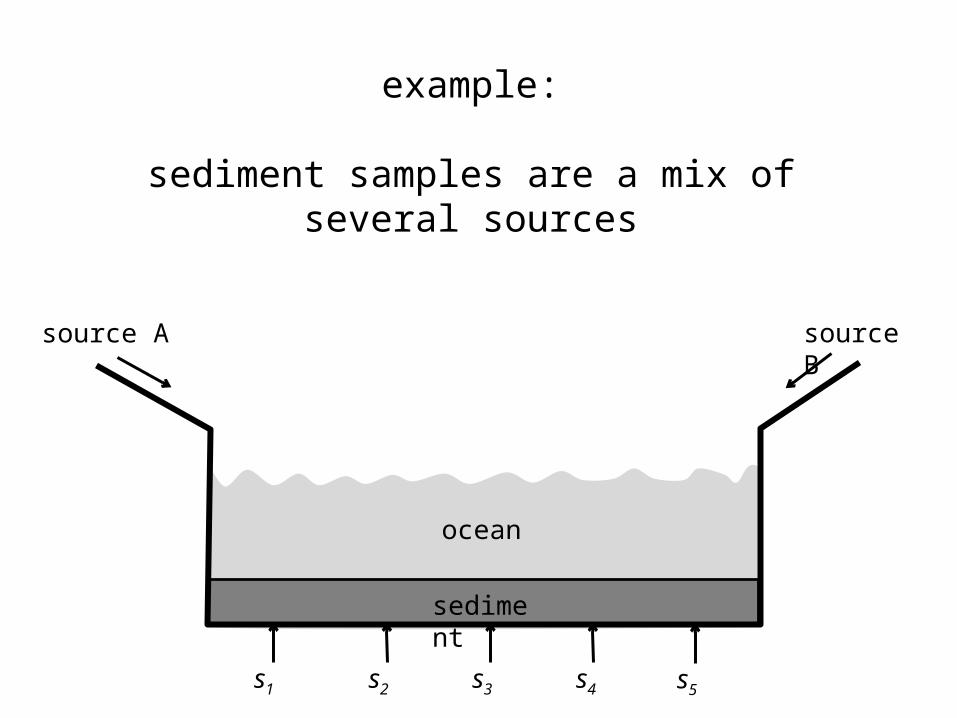
source A

ocean

sediment

source B

s4s2 s3s1 s5

example:

sediment samples are a mix of several sources

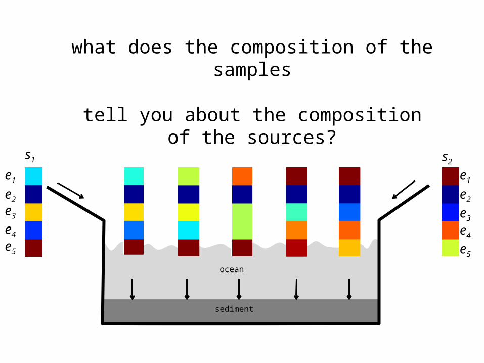
e1e2e3e4e5

e1e2e3e4e5

s1 s2

ocean

sediment

what does the composition of the samples

tell you about the composition of the sources?

another example

Atlantic Rock Datasetchemical composition for several thousand rocks

Rocks are a mix of minerals, and …

mineral 1mineral 2mineral 3

rock 1 rock 2rock 3

rock 4

rock 5 rock 6 rock 7

…minerals have a well-defined composition

Which simpler?

rocks have a chemical composition

or

rocks contain minerals

and

minerals have chemical compositions

answer will depend on how many minerals are involved

and how many elements are in each mineral

representing mixing with matrices

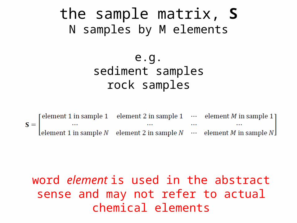
the sample matrix, SN samples by M elements

e.g.sediment samples

rock samples

word element is used in the abstract sense and may not refer to actual chemical elements

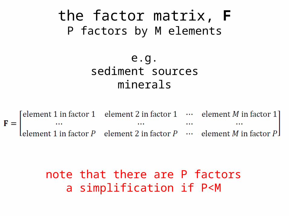
the factor matrix, FP factors by M elements

e.g.sediment sources

minerals

note that there are P factorsa simplification if P<M

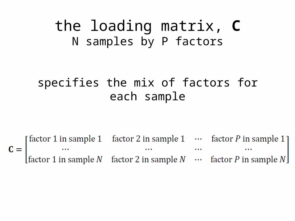
the loading matrix, CN samples by P factors

specifies the mix of factors for each sample

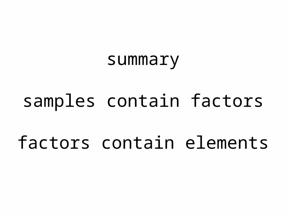
summary

samples contain factors

factors contain elements

an important issue

how many factors are needed to represent the samples?

need at most P=Mbut is P < M ?

simple example using ternary diagrams

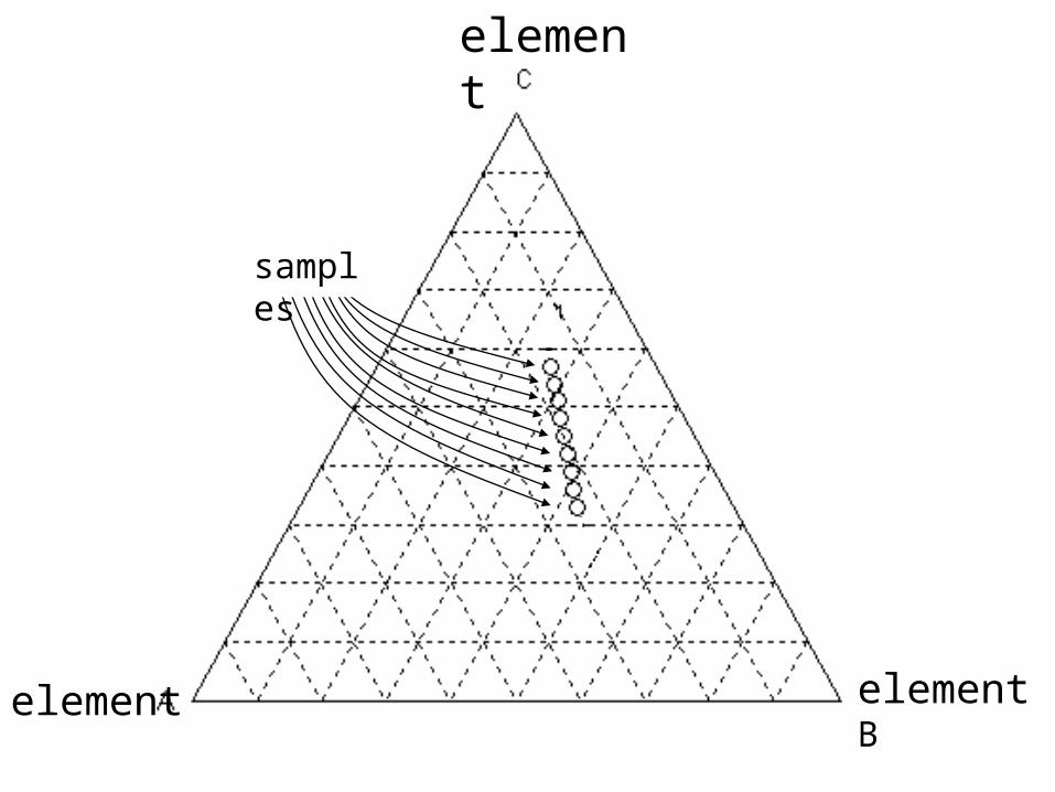
samples

element

element element B

samples

element

element element B

line of samples implies only 2 factors, so P=2

factorssamples

element

element element B

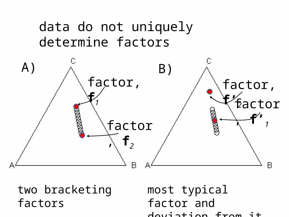
A) B)factor, f’2

factor, f’1

factor, f1

factor, f2

data do not uniquely determine factors

two bracketing factors most typical factor and deviation from it

mathematically

S = CF = C’ F’with F’ = M F and C’ = C M-1 where M is any P×P matrix with an inverse

must rely on prior information to choose M

a method to determine

the minimum number of factors, Pand

one possible set of factors

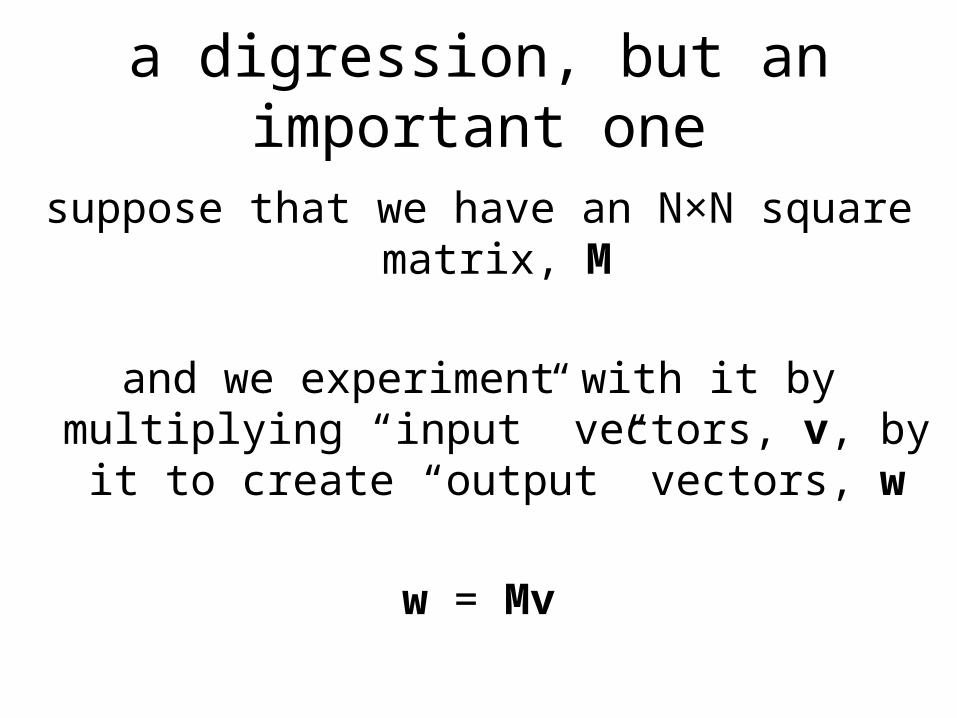
a digression, but an important one

suppose that we have an N×N square matrix, Mand we experiment with it by multiplying “input”

vectors, v, by it to create “output” vectors, ww = Mv

surprisingly, the answer to the question

when is the output parallel to the input ?

tells us everything about the matrix

if w is parallel to vthenw = λ v

where λ is a proportionality factor

the equationw = Mv is then λ v = Mv or (M - λ I)v=0

but if (M - λ I)v=0then it would seem that

v = (M - λ I)-10 = 0 which is not a very interesting solutionw is parallel to v when v is zero

to make an interesting solution you must choose λ so that

(M - λ I)-1 doesn’t exist

which is equivalent to choosing λ so that

det(M - λ I)=0

to make an interesting solution you must choose λ so that

(M - λ I)-1 doesn’t exist

which is equivalent to choosing λ so that

det(M - λ I)=0

since a matrix with zero

determinant has no inverse

in the 2×2 case …

this is a quadratic equation in λand so has two solutionsλ1 and λ 2

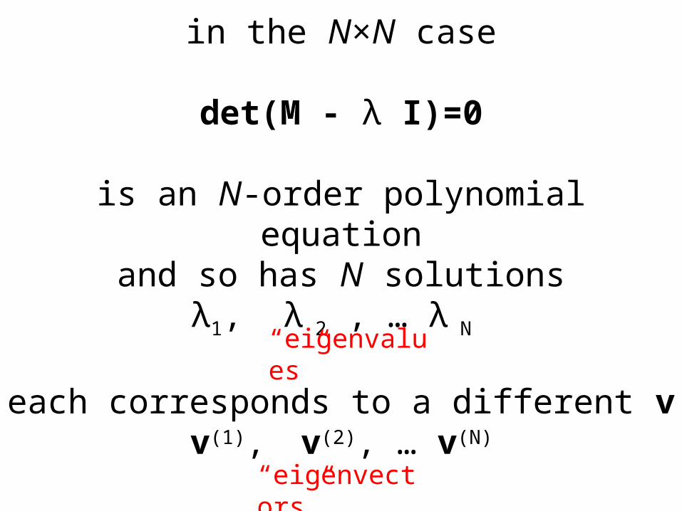
in the N×N case

det(M - λ I)=0

is an N-order polynomial equationand so has N solutionsλ1, λ 2 , … λ N

each corresponds to a different vv(1), v(2), … v(N)

in the N×N case

det(M - λ I)=0

is an N-order polynomial equationand so has N solutionsλ1, λ 2 , … λ N

each corresponds to a different vv(1), v(2), … v(N)“eigenvalues”

“eigenvectors”

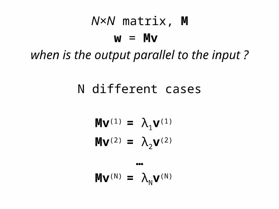
N×N matrix, Mw = Mv when is the output parallel to the input ?

N different cases

Mv(1) = λ1v(1) Mv(2) = λ2v(2) …Mv(N) = λNv(N)

Mv(1) = λ1v(1) Mv(2) = λ2v(2) …Mv(N) = λNv(N) simplify notationMV = V Λ

In the text its shown thatif M is symmetric

then

all λ’s are real

v’s are orthonormal

v(i)T v(j) = 1 if i=j0 if i ≠ j

In the text its shown thatif M is symmetric

then

all λ’s are real

v’s are orthonormal

v(i)T v(j) = 1 if i=j0 if i ≠ j

implies VTV = VVT= I

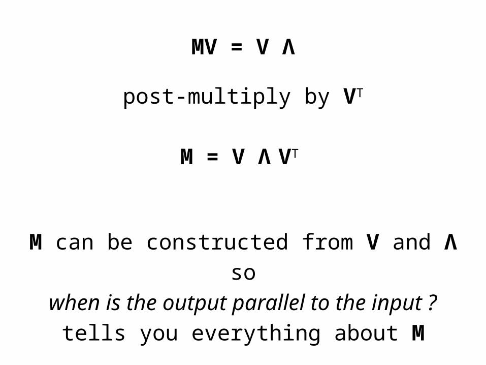
MV = V Λpost-multiply by VT

M = V Λ VT

M can be constructed from V and Λso

when is the output parallel to the input ?

tells you everything about M

now here’s what this has to do with factors

suppose S is square and symmetricthen

S = CF = V Λ VT

suppose S is square and symmetricthen

S = CF = V Λ VTC F

suppose S is square and symmetricthen

S = CF = V Λ VTC F

S can be represented by M mutually-perpendicular factors, F

furthermore, suppose that only P eigvenvalues are nonzero

the eigenvectors with zero eigenvalues can be thrown out of the equation

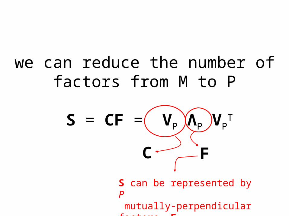
we can reduce the number of factors from M to P

S = CF = VP ΛP VPTC F

S can be represented by P mutually-perpendicular factors, FP

unfortunately …

Sis usually neither square nor symmetric

so a patch in the methodology is needed

the trick …

STSis an M×M square matrix

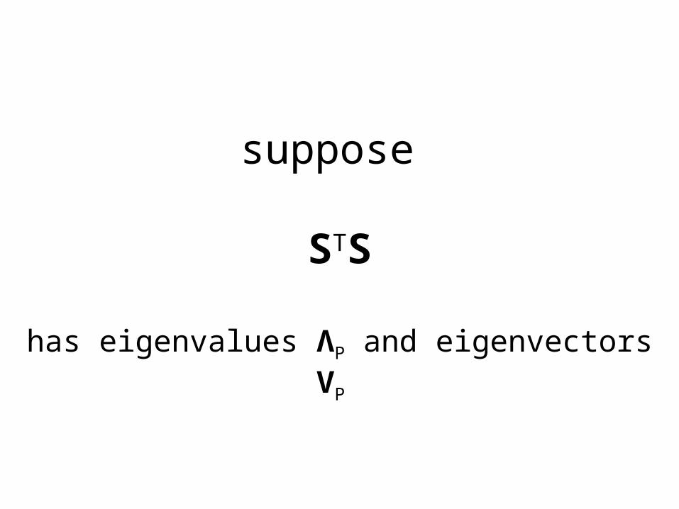
suppose

STShas eigenvalues ΛP and eigenvectors VP

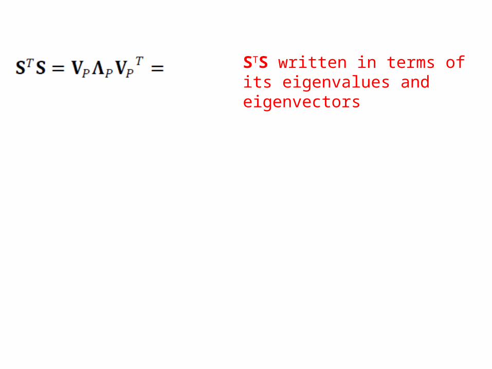
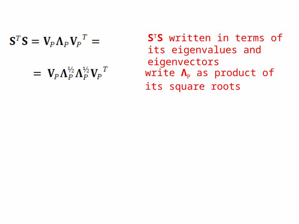
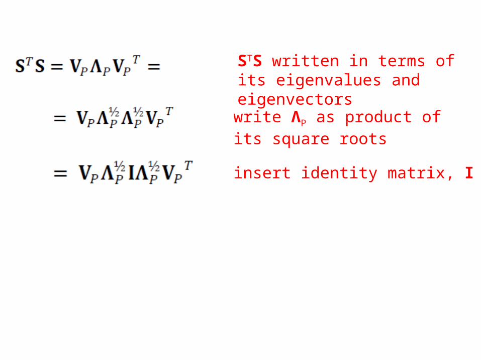
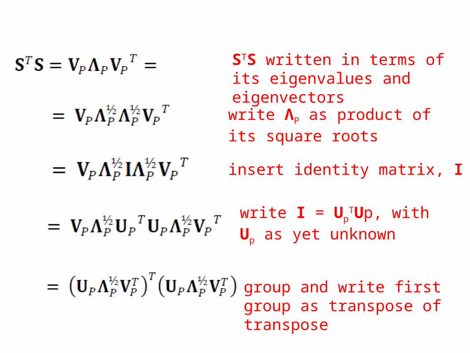
STS written in terms of its eigenvalues and eigenvectors

STS written in terms of its eigenvalues and eigenvectors

write ΛP as product of its square roots

STS written in terms of its eigenvalues and eigenvectors

write ΛP as product of its square roots insert identity matrix, I

STS written in terms of its eigenvalues and eigenvectors

write ΛP as product of its square roots

write I = UpTUp, with Up as yet unknown

insert identity matrix, I

STS written in terms of its eigenvalues and eigenvectors

write ΛP as product of its square roots

write I = UpTUp, with Up as yet unknown

insert identity matrix, I

group and write first group as transpose of transpose

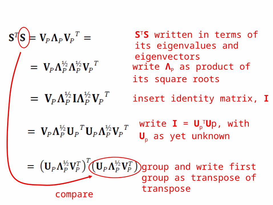
STS written in terms of its eigenvalues and eigenvectors

write ΛP as product of its square roots

write I = UpTUp, with Up as yet unknown

insert identity matrix, I

group and write first group as transpose of transpose

compare

so

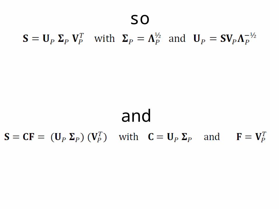
and

so

and

so

called the “singular value decomposition” of S

now the non-square, non-symmetric matrix, S, is represented as a mix of P

mutually perpendicular factors

called the “singular values”

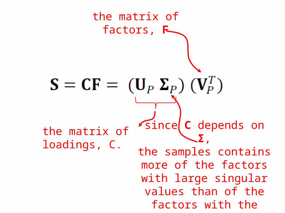
the matrix of loadings, C.

the matrix of factors, F

since C depends on Σ,the samples contains more of the factors with large singular values than of the factors with

the small singular values

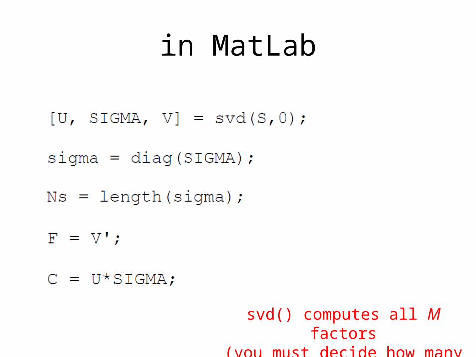
in MatLab

svd() computes all M factors(you must decide how many to use)

1 2 3 4 5 6 7 80

1000

2000

3000

4000

5000singular values, s(i)

index, i

s(i)

sing

ular

val

ues,

Sii

index, i

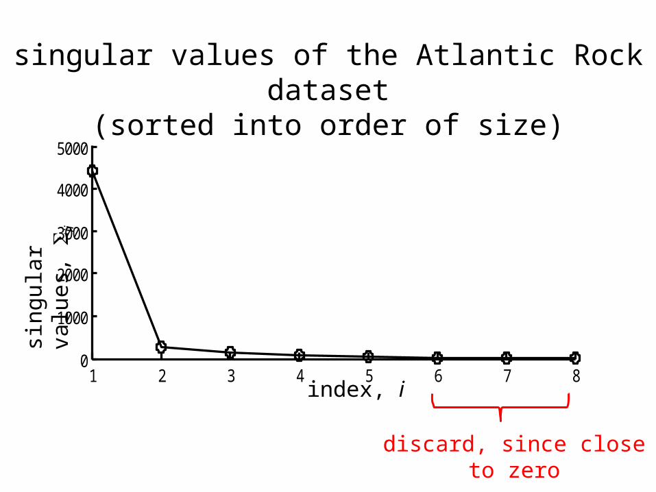
singular values of the Atlantic Rock dataset(sorted into order of size)

1 2 3 4 5 6 7 80

1000

2000

3000

4000

5000singular values, s(i)

index, i

s(i)

sing

ular

val

ues,

Sii

index, i

singular values of the Atlantic Rock dataset(sorted into order of size)

discard, since close to zero

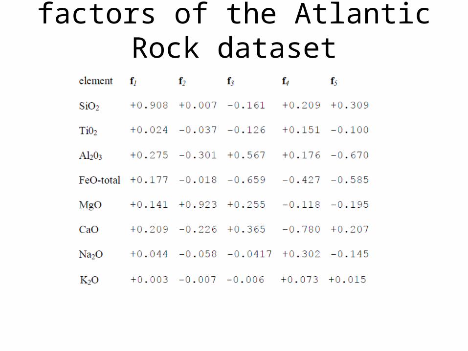
factors of the Atlantic Rock dataset

factor of the Atlantic Rock dataset

factor 1 is the “typical factor”

factor of the Atlantic Rock dataset

factor 2 as MgO increases, Al2O3 and CaO decreases

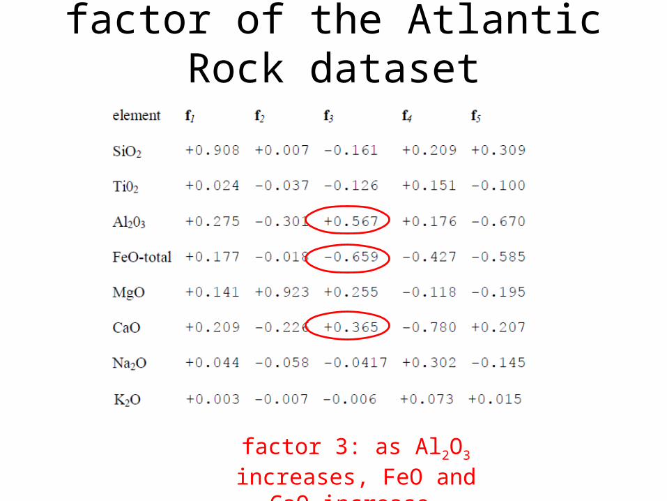
factor of the Atlantic Rock dataset

factor 3: as Al2O3 increases, FeO and CaO increase

f2 f3 f4 f5

f2p f3p f4p f5p

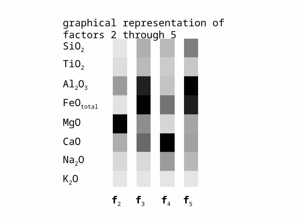
graphical representation of factors 2 through 5

f5f2 f3 f4

SiO2

TiO2

Al2O3

FeOtotal

MgO

CaO

Na2O

K2O

C2

C3

C4

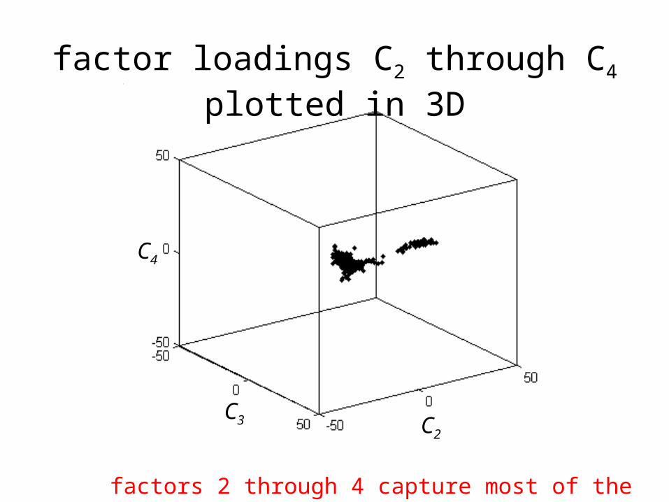
factor loadings C2 through C4 plotted in 3D

factors 2 through 4 capture most of the variability of the rocks

Al203

Ti02Al203

Si02

K20

Fe0

Mg0

Al203

A) B)

C) D)