Environmental Hydraulics of Open Channel Flows

This page intentionally left blank

Environmental Hydraulics of Open Channel Flows

Hubert ChansonME, ENSHM Grenoble, INSTN, PhD (Cant), DEng (Qld)

Eur Ing, MIEAust, MIAHR13th Arthur Ippen awardee (IAHR)

Reader in Environmental Fluid Mechanics and Water Engineering

The University of Queensland, AustraliaE-mail: h.chanson@uq.edu.au

Web site: http://www.uq.edu.au/~e2hchans/

AMSTERDAM BOSTON HEIDELBERG LONDON NEW YORK OXFORD PARIS SAN DIEGO SAN FRANCISCO SINGAPORE SYDNEY TOKYO

Elsevier Butterworth-HeinemannLinacre House, Jordan Hill, Oxford OX2 8DP

200 Wheeler Road, Burlington, MA 01803

First published 2004

Copyright © 2004, Hubert Chanson. All rights reserved

The right of Hubert Chanson to be identified as the author of this work has been asserted in accordance with the Copyright, Designs and Patents Act 1988

No part of this publication may be reproduced in any material form (including photocopying or storing in any medium by electronic means and whether or not transiently or incidentally to some other use of this publication) without the written permission of the copyright holder except in accordance with the provisions of the Copyright, Designs and Patents Act 1988 or under the terms

of a licence issued by the Copyright Licensing Agency Ltd, 90 Tottenham Court Road, London, England W1T 4LP. Applications for the copyright

holder’s written permission to reproduce any part of this publication should be addressed to the publisher

Permissions may be sought directly from Elsevier’s Science & Technology Rights Department in Oxford, UK: phone: (+44) 1865 843830,

fax: (+44) 1865 853333, e-mail: permissions@elsevier.co.uk. You may also complete your request on-line via the

Elsevier homepage (http://www.elsevier.com), by selecting ‘Customer Support’ and then ‘Obtaining Permissions’

British Library Cataloguing in Publication DataA catalogue record for this book is available from the British Library

Library of Congress Cataloguing in Publication DataA catalogue record for this book is available from the Library of Congress

ISBN: 0 7506 6165 8

For information on all Elsevier Butterworth-Heinemann publicationsvisit our web site at http://books.elsevier.com

Typeset by Charon Tec Pvt. Ltd, Chennai, IndiaPrinted and bound in Great Britain

Contents

Preface ixAcknowledgements xviAbout the author xviiiDedication xxiGlossary xxiiList of symbols xlv

Part 1 Introduction to Open Channel Flows 1

1. Introduction 31.1 Presentation 31.2 Fluid properties 51.3 Fluid statics 61.4 Open channel flows 71.5 Exercises 10

2. Fundamentals of open channel flows 112.1 Presentation 112.2 Fundamental principles 152.3 Open channel hydraulics of short, frictionless transitions 192.4 The hydraulic jump 242.5 Open channel flow in long channels 262.6 Summary 332. Exercises 34

Part 2 Turbulent Mixing and Dispersion in Rivers and Estuaries:An Introduction 35

3. Introduction to mixing and dispersion in natural waterways 373.1 Introduction 373.2 Laminar and turbulent flows 403.3 Basic definitions 443.4 Structure of the section 453.5 Appendix A – Application: buoyancy force exerted on a submerged

air bubble 463.6 Appendix B – Freshwater properties 483.7 Exercises 483.8 Exercise solutions 48

4. Turbulent shear flows 494.1 Presentation 494.2 Jets and wakes 53

7

4.3 Boundary layer flows 544.4 Fully developed open channel flows 584.5 Mixing in turbulent shear flows 604.6 Exercises 634.7 Exercise solutions 64

5. Diffusion: basic theory 655.1 Basic equations 655.2 Applications 675.3 Appendix A – Mathematical aids 725.4 Exercises 745.5 Exercise solutions 74

6. Advective diffusion 756.1 Basic equations 756.2 Basic applications 766.3 Two- and three-dimensional applications 796.4 Exercises 806.5 Exercise solutions 80

7. Turbulent dispersion and mixing: 1. Vertical and transverse mixing 817.1 Introduction 817.2 Flow resistance in open channel flows 837.3 Vertical and transverse (lateral) mixing in turbulent river flows 847.4 Turbulent mixing applications 887.5 Discussion 917.6 Appendix A – Friction factor calculations 937.7 Appendix B – Random walk model 937.8 Appendix C – Turbulent mixing in hydraulic jumps and bores 957.9 Exercises 977.10 Exercise solutions 97

8. Turbulent dispersion and mixing: 2. Longitudinal dispersion 998.1 Introduction 998.2 One-dimensional turbulent dispersion 1008.3 Longitudinal dispersion in natural streams 1018.4 Approximate models for longitudinal dispersion 1068.5 Design applications 1098.6 Exercises 1118.7 Exercise solutions 113

9. Turbulent dispersion in natural systems 1179.1 Introduction 1179.2 Longitudinal dispersion in natural rivers with dead zones 1209.3 Dispersion and transport of reactive contaminants 1279.4 Transport with reaction 1309.5 Appendix A – Air–water mass transfer in air–water flows 1369.6 Appendix B – Solubility of nitrogen, oxygen and argon in water 138

vi Contents

9.7 Appendix C – Molecular diffusion coefficients in water (after Chanson 1997a) 139

9.8 Exercises 1409.9 Exercise solutions 141

10. Mixing in estuaries 14410.1 Presentation 14410.2 Basic mechanisms 14910.3 Applications 15910.4 Turbulent mixing and dispersion coefficients in estuaries 16410.5 Applications 16510.6 Appendix A – Observations of mixing and dispersion coefficients

in estuarine zones 17110.7 Exercises 17310.8 Exercise solutions 175

Part 2 Revision exercises 177Assignment solutions 179

Part 3 Introduction to Unsteady Open Channel Flows 183

11. Unsteady open channel flows: 1. Basic equations 18511.1 Introduction 18511.2 Basic equations 18911.3 Method of characteristics 19811.4 Discussion 21111.5 Exercises 21711.6 Exercise solutions 219

12. Unsteady open channel flows: 2. Applications 22312.1 Introduction 22312.2 Propagation of waves 22412.3 The simple wave problem 22712.4 Positive and negative surges 23312.5 The kinematic wave problem 24712.6 The diffusion wave problem 24912.7 Appendix A – Gaussian error functions 25512.8 Exercises 25612.9 Exercise solutions 258

13. Unsteady open channel flows: 3. Application to dam break wave 26313.1 Introduction 26313.2 Dam break wave in a horizontal channel 26813.3 Effects of flow resistance 27813.4 Embankment dam failures 28613.5 Related flow situations 29313.6 Exercises 29913.7 Exercise solutions 300

Contents vii

14. Numerical modelling of unsteady open channel flows 30214.1 Introduction 30214.2 Explicit finite difference methods 30614.3 Implicit finite difference methods 31214.4 Exercises 315

Part 3 Revision exercises 316Revision exercise no. 1 316Revision exercise no. 2 316Revision exercise no. 3 319Revision exercise no. 4 320

Part 4 Interactions between Flowing Water and its Surroundings 323

15. Interactions between flowing water and its surroundings: introduction 32515.1 Presentation 32515.2 Terminology 33015.3 Structure of this section 330

16. Interaction between flowing water and solid boundaries: sediment processes 33116.1 Introduction 33116.2 Physical properties of sediments 33316.3 Threshold of sediment bed motion 33516.4 Sediment transport 33916.5 Total sediment transport rate 34116.6 Exercises 347

17. Interaction between flowing water and free surfaces: self-aeration and air entrainment 34817.1 Introduction 34817.2 Free-surface aeration in turbulent flows: basic mechanisms 34817.3 Dimensional analysis and similitude 35817.4 Basic metrology in air–water flow studies 36417.5 Applications 37317.6 Appendix A – Air bubble diffusion in plunging jet flows

(after Chanson 1997a) 38417.7 Appendix B – Air bubble diffusion in self-aerated supercritical flows 38917.8 Appendix C – Air bubble diffusion in high-velocity water jets 39317.9 Exercises 396

Appendix A: Constants and fluid properties 399Appendix B: Unit conversions 403

References 406Abbreviations of journals and institutions 420Common bibliographical abbreviations 421

Index 423

viii Contents

Preface

Rivers play a major role in shaping the landscapes of our planet (Table P.1, Fig. P.1). Extremeflow rates may vary from zero in drought periods to huge amount of waters in flood periods.For example, the maximum observed flood discharge of the Amazon River at Obidos wasabout 370 000 m3/s (Herschy 2002). This figure may be compared with the average annual dis-charges of the Congo River (41 000 m3/s at the mouth) and of the Murray-Darling River(0.89 m3/s at the mouth) (Table P.1). Even arid, desertic regions are influenced by fluvial actionwhen periodic flood waters surge down dry watercourses (Fig. P.1(a)).

Hydraulic engineers have had an important role to contribute although the technical chal-lenges are gigantic, often involving multiphase flows and interactions between fluids and bio-logical life. These engineers were at the forefront of science for centuries. For example, thearts of tapping groundwater developed early in the Antiquity in Armenia and Persia, theRoman aqueducts, and the Grand canal navigation system in China. In the author’s opinion,the extreme complexity of hydraulic engineering is closely linked with:

1. The geometric scale of water systems: e.g. from �10 m2 for a soil erosion pattern (e.g. rill) to over 1000 km2 for a river catchment area typically, and ocean surface area over 1 � 106km2.

2. The broad range of relevant time scales: e.g. �1 s for a breaking wave, about 1 � 104s fortidal processes, about 1 � 108s for reservoir siltation, and about 1 � 109s for deep seacurrents.

Table P.1 Characteristics of the world’s longest rivers

River system Length Catchment Average annual Average sediment(km) area discharge transport rate

(km2) (m3/s) (tons/day)(1) (2) (3) (4) (5)

Amazon-Ucayali-Apurimac (South America) 6400 6 000 000 180 000 1 300 000Congo (Africa) 4700 3 700 000 41 000 –Yangtze (Asia) 6300 1 808 500 31 000 –Yenisey-Baikal-Selenga (Asia) 5540 2 580 000 19 800 –Parana (South America) 4880 2 800 000 17 293 –Mississippi-Missouri-Red Rock 5971 3 100 00 17 000 –

(North America)Ob-Irtysh (Asia) 5410 2 975 000 12 700 –Amur-Argun (Asia) 4444 1 855 000 10 900 –Volga (Europe) 3530 1 380 000 8050 –Nile (Africa) 6650 3 349 000 3100 –Huang Ho (Yellow River) (Asia) 5464 752 000 1840 4 400 000Murray-Darling (Australia) 3370 1 072 905 0.89 –

Average annual discharge: at the river mouth.

x Preface

(a)

(b)

Fig. P.1 Photographs of natural rivers. (a) Small flood in the Gascoyne River, Carnarvon, WA (Australia) (courtesy ofGascoyne Development Commission and Robert Panasiewicz). The Gascoyne River has catchment area of about67 770 km2 and it extends 630 km inland. Average annual rainfall is �250 mm throughout the basin and this is anephemeral river. There are typically one to two flow periods per year following seasonal rainfall or cyclone activity,but it may fails to flow at all once every 5 or 6 years. (b) Tingalpa Creek, Redlands Qld (Australia) on 21 January 2003at high tide at about 9 km from the river mouth, looking upstream.

3. The variability of river flows from zero (dry river bed during droughts) to gigantic floods.4. The complexity of basic fluid mechanics, with governing equations characterized by

non-linearity, natural fluid instabilities, interactions between water, solid, air and bio-logical life and;

5. Man’s (and Life’s) total dependence on water.

Preface xi

DISCUSSIONArmed conflicts around water systems have been plenty. In the Bible, a wind-setup effectallowed Moses and the Hebrews to cross shallow-water lakes and marshes during their exo-dus. Droughts were artificially introduced: e.g. during the siege of the ancient city of KharaKhoto (Black City) in AD 1372, the Chinese army diverted the Ezen River1 supplying water tothe city.2 Man-made flooding3 of an army or a city was carried out by the Assyrians (Babylon,Iraq BC 689), the Spartans (Mantinea, Greece BC 385–384), the Chinese (Huai River, AD

514–515).4 A related case was the air raids of the dam buster campaign conducted by theBritish in 1943. Artifical flooding created by dyke destruction played a role in several wars:e.g. the war between the cities of Lagash and Umma (Assyria) around BC 2500 was fought forthe control of irrigation systems and dykes.

The 21st Century is facing political instabilities centred around water systems, and freshwater system issues might be the focal point of future armed conflicts. For example,the Tigris and Euphrates River catchments and the Mekong River. The scope of the relevantproblems is broad and complex: e.g. water quality, pollution, flooding and drought. Anexample is the disaster of the Aral Sea with the formation of the permanently-dry isthmusbetween the northern small Aral Sea and the southern big Aral Sea since 1987 (Walthamand Sholji 2001).

This book was developed to introduce students, professionals and managers to the challengesof open channel flows and environmental hydraulics. After a concise introduction (Part 1),the second section (Part 2) deals with mixing and dispersion of matter in natural river sys-tems. Part 3 presents an introduction to unsteady open channel flows, and the interactionsbetween flowing water and its surroundings are discussed in Part 4.

Mixing and dispersion of contaminants in natural systems are developed in Part 2.Applications include release of organic and nutrient-rich waste water into the ecosystem (e.g.from treated sewage effluent), smothering of seagrass and coral, storm water runoff duringflood events, and injection of heated water from an industrial discharge (e.g. at a coolingpower plant). For example, during an accidental release of waste occurs in a stream, the waterresource scientist needs to predict the arrival time of the contaminant cloud, the peak con-centration of solute and the duration of the pollution. Basic theory of molecular diffusion andadvection is extended to turbulent advective diffusion in channels.

Gradually varied flow calculations are developed in Part 3. First the basic equations of one-dimensional unsteady open channel flows are presented. That is, the Saint-Venant

1Also called Hei He River (Black River) by the Chinese.2Located in the Gobi Desert, Khara Khoto was ruled by the Mongol King Khara Bator (Webster 2002).3By building an upstream dam and destroying it.4 It may be added the aborted attempt to blow up Ordunte Dam, during the Spanish Civil War, by the troops ofGeneral Franco, and the anticipation of German Dam destruction at the German–Swiss border to stop the crossingof the Rhine River by the Allied Forces in 1945.

equations and the method of characteristics in Chapter 11*. Later simple applications aredeveloped. The propagation of waves, and positive and negative surges is presented inChapter 12, while the dam break wave problem is discussed in Chapter 13. Simple numericalmodels are presented and explained in Chapter 14.

There are strong interactions between turbulent water flows and the surrounding environ-ment. Part 4 introduces the basic concepts of the transport of solids (Chapter 16), and of themixing of air and water at free surfaces (Chapter 17).

At the beginning of the book, the reader will find the table of contents, a list of symbols anda glossary of technical terms and names. After the conclusion, a detailed list of references ispresented. The last section presents a correction form. Readers who find an error or mistake arewelcome to record the error on the page and to send a copy to the author. Corrections andupdates will be posted on the Internet at: http://www.uq.edu.au/�e2hchans/reprints/book7.htm

DiscussionThe lecture material is based upon the author’s experience at the University of Queensland,and at other universities. It is designed primarily for undergraduate students in civil, envi-ronmental and hydraulic engineering. The author has taught Part 1 in Years 2 and 3, and Parts2 and 3 as parts of advanced undergraduate electives in Year 4. Some material of Part 4 is usually introduced in the advanced hydraulics elective subject, and the course is furtherdeveloped at postgraduate levels.

The author wants to stress, however, that field studies are a necessary complement to traditional lectures in environmental hydraulics. In the context of undergraduate subjects,design applications in classroom are restricted to simple flow situations and boundary condi-tions for which the basic equations can be solved analytically or with simple models.Fieldwork activities (Fig. P.2) are essential to illustrate real professional situations, and thecomplex interactions between all engineering and non-engineering constraints.

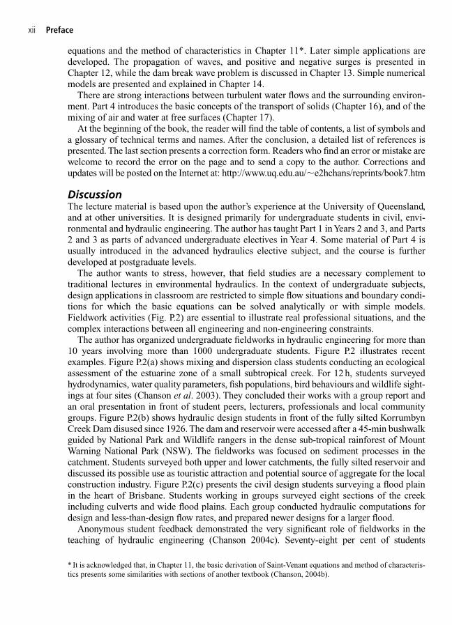
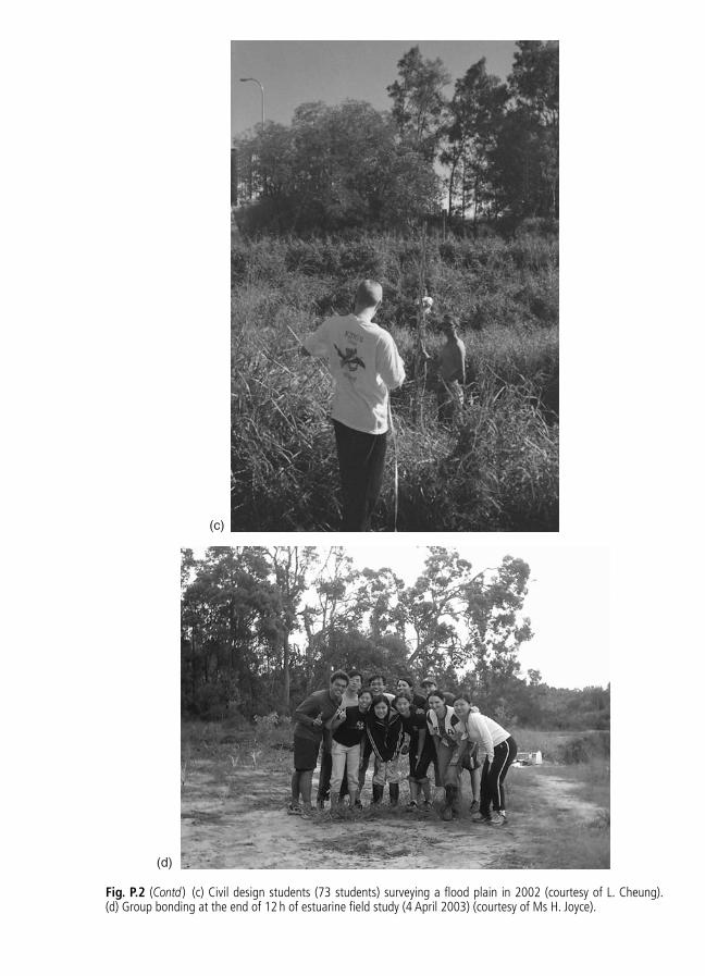
The author has organized undergraduate fieldworks in hydraulic engineering for more than10 years involving more than 1000 undergraduate students. Figure P.2 illustrates recent examples. Figure P.2(a) shows mixing and dispersion class students conducting an ecologicalassessment of the estuarine zone of a small subtropical creek. For 12 h, students surveyedhydrodynamics, water quality parameters, fish populations, bird behaviours and wildlife sight-ings at four sites (Chanson et al. 2003). They concluded their works with a group report andan oral presentation in front of student peers, lecturers, professionals and local communitygroups. Figure P.2(b) shows hydraulic design students in front of the fully silted KorrumbynCreek Dam disused since 1926. The dam and reservoir were accessed after a 45-min bushwalkguided by National Park and Wildlife rangers in the dense sub-tropical rainforest of MountWarning National Park (NSW). The fieldworks was focused on sediment processes in thecatchment. Students surveyed both upper and lower catchments, the fully silted reservoir anddiscussed its possible use as touristic attraction and potential source of aggregate for the localconstruction industry. Figure P.2(c) presents the civil design students surveying a flood plainin the heart of Brisbane. Students working in groups surveyed eight sections of the creekincluding culverts and wide flood plains. Each group conducted hydraulic computations fordesign and less-than-design flow rates, and prepared newer designs for a larger flood.

Anonymous student feedback demonstrated the very significant role of fieldworks in theteaching of hydraulic engineering (Chanson 2004c). Seventy-eight per cent of students

xii Preface

* It is acknowledged that, in Chapter 11, the basic derivation of Saint-Venant equations and method of characteris-tics presents some similarities with sections of another textbook (Chanson, 2004b).

(a)

(b)

Fig. P.2 Photographs of undergraduate student field trips. (a) Mixing in estuary fieldwork (39 students) at EprapahCreek on 4 April 2003, students conducting sampling tests in the mangrove (courtesy of Ms H. Joyce). (b) Field study on4 September 2002 with hydraulic design class (24 students), students in front of the fully silted Korrumbyn Creek Damin a dense sub-tropical rainforest.

(c)

(d)

Fig. P.2 (Contd ) (c) Civil design students (73 students) surveying a flood plain in 2002 (courtesy of L. Cheung).(d) Group bonding at the end of 12 h of estuarine field study (4 April 2003) (courtesy of Ms H. Joyce).

believed strongly and very strongly that ‘fieldwork is an important component of the subject’.Eighty-four per cent of students agreed strongly and very strongly that ‘all things considered,fieldworks and site visits are the vital components of civil and environmental engineering curricula’. Ninety-six per cent of students believed that ‘fieldworks play a vital role to compre-hend real-word engineering’and 100% of interviewed employers stressed that fieldworks underacademic supervision was a basic requirement for civil and environmental engineering gradu-ates. Lecturers and professionals should not be complaisant with university hierarchy andadministration clerks to cut costs by eliminating field studies. Although the preparation andorganization of fieldworks with large class sizes are a major effort, the outcome is very reward-ing for the students and the lecturer. From his own experience, the author has had great pleas-ure in bringing his students to hydraulics fieldwork for more than a decade and to experiencefirst hand their personal development (Fig. P.2(d)).

Internet resourcesGeneral resourcesGallery of photographs http://www.uq.edu.au/�e2hchans/photo.htmlReprints of research papers http://www.uq.edu.au/�e2hchans/reprints.htmlInternet technical resources http://www.uq.edu.au/�e2hchans/url_menu.htmlNASA Earth observatory http://earthobservatory.nasa.gov/NASA rain, wind and air-sea gas http://bliven2.wff.nasa.gov/index.htmexchange research USACE inlets online http://www.oceanscience.net/inletsonline/Estuaries in South Africa http://www.upe.ac.za/cerm/Whirlpools http://www.uq.edu.au/�e2hchans/whirlpl.html

Mixing and dispersion in riversRivers seen from space http://www.athenapub.com/rivers1.htmAerial photographs of rivers ftp://geology.wisc.edu/pub/air

Preface xv

Acknowledgments

The author wants to thank Prof. Colin J. Apelt, University of Queensland, for his help, supportand assistance all along the academic career of the author, and Dr Jean Cunge who presentedsome superb lectures. The author thanks particularly his friend Prof. Shin-ichi Aoki,Toyohashi University of Technology (Japan) for his valuable advice and comments.

The author thanks his research students who conducted relevant experimental work: Ms Chantal Donnelly, Dr Carlos Gonzalez, Ms Karen Hickox, Mr Chung Hwee Jerry Lim,Mr Mamuro Maruyama, Ms Claire Quinlan, Mr Chye-Guan Sim, Mr Frankie Tan, Mr York-WeeTan and Dr Luke Toombes.

The author wishes to express his gratitude to the followings who made available some photographs of interest:

Acres International, Canada;Mr Amir Aghakoochak, Iran;Michael Armitage, University of Sheffield, UK;Dr Marie Augendre, Université de Lyon 2, France;Dr Antje Bornschein, University of Dresden, Germany;Mr and Mrs Chanson, France;Consortium for Estuarine Research and Management (CERM), South Africa;Coastal and Hydraulics Laboratory, US Army Corps of Engineers;Prof. Andre Fourie, University of Witwatersrand, South Africa;Gascoyne Development Commission, WA, Australia;Dr Michael R. Gourlay, Brisbane, Australia;Gary & Rhonda Higgins, Northern Territory, Australia;Lim Hiok Hwa, Department of Irrigation and Drainage, Sarawak, Indonesia;Dr Eric Jones, Proudman Oceanographic Laboratory, UK;Pr J. Knauss, Münich University of Technology, Germany;Ms Sasha Kurz, Brisbane, Australia;Ms Nathalie Lemiere, Sequana-Normandie, France;Mr Jerry Lim, Singapore;Dr Pedro Lomonaco, University of Cantabria, Spain;Dr Lou Maher, University of Wisconsin, USA;Dr John Macintosh, Water Solutions, Australia;Dr Richard Manasseh, CSIRO, Australia;Mr Dennis Murphy, USA;Prof. Okada, Mt Usu Vulcano Observatory. Hokudai Faculty of Science, Japan;Mr Robert Panasiewicz, Gascoyne Development Commission, Australia;Prof. D. Howell Peregrine, University of Bristol, UK;Mr Bruno de Quinsonas, Le Touvet, France;Mr Marq Redeker, Ruhrverband, Germany;

The Santa Clarita Valley Historical Society, California, USA;Mr Chye-Guan Sim, Singapore;Daniel Stephens, USA;Mr Frankie Tan, Singapore;Mr York-Wee Tan, Singapore;Tonkin and Taylor, New Zealand;Mr Didier Toulouze, Fréjus, France;US Army Corps of Engineers, Portland district;US Naval Historical Center, USA;Waterways Scientific Services, Queensland Environmental Protection Agency, Australia;Prof. Steven J. Wright, University of Michigan, USA.

The author thanks the following people in providing relevant experimental data:

Prof. S. Aoki, Toyohashi University of Technology, Japan;Dr I. Ramsay, Queensland Environmental Protection Agency, Australia;Dr Y. Yasuda, Nihon University, Japan.

The author thanks also the following people in providing additional information: Prof.Shin-ichi Aoki (Japan); Dr Richard Brown, QUT (Australia); Dr Antje Bornschein, Universityof Dresden (Germany); Mr and Mrs Chanson (France); Dr Stephen Coleman, University ofAuckland (New Zealand); Dr Peter Cummings (Australia); Mr John Ferris, Qld EPA (Australia);John Grimston (New Zealand); Dr Eric Jones, Proudman Oceanographic Laboratory (UK);Prof. Iwao Ohtsu, Nihon University (Japan); Robert Panasiewicz, Gascoyne DevelopmentCommission (Australia); Dr Ian Ramsay, Qld EPA (Australia); John Remi (Canada); Mr M. Tomkins (Australia); Dr Youichi Yasuda, Nihon University (Japan).

The help and assistance of the following colleagues must be acknowledged: Prof. C.J. Apelt and Dr P. Nielsen.

At last but not the least, the author thanks all the people (including colleagues, former students, students and professionals) who gave him information, feedback and comments onhis lecture material. In particular, some material on the Saint-Venant equations and themethod of characteristics derived from Dr Jean Cunge’s lecture notes.

Acknowledgments xvii

About the author

Hubert Chanson is a Reader in Environmental Fluid Mechanics and Water Engineering at theUniversity of Queensland since 1990. He was born in 1961 in Paris, France. He lives inBrisbane, Australia, with his wife Ya-Hui (Karen) Chou and their children Bernard and Nicole.He received a degree of ‘Ingénieur Hydraulicien’ from the Hydraulic Engineering School of Grenoble, France (ENSHMG) in 1983 and a postgraduate degree of ‘Ingénieur GénieAtomique’ from the Nuclear Engineering Institute of Saclay (INSTN) in 1984. He worked forthe industry in France as an R&D Engineer at the Atomic Energy Commission from 1984 to1986, and as a computer professional in fluid mechanics for Thomson-CSF between 1989 and1990. From 1986 to 1988, he studied at the University of Canterbury (New Zealand) as part ofa PhD project. He was awarded a Doctor of Engineering from the University of Queensland in 1999 for outstanding research achievements in gas–liquid bubbly flows. In 2003, theInternational Association for Hydraulic engineering and Research (IAHR) presented him the13th Arthur Ippen Award for outstanding achievements in hydraulic engineering. This award isregarded as the highest achievement in hydraulic research.

His research interests cover design of hydraulic structures, experimental investigations of two-phase flows, coastal hydrodynamics, water quality modelling, environmental man-agement and natural resources. He authored several books: Hydraulic Design of SteppedCascades, Channels, Weirs and Spillways (Pergamon, 1995), Air Bubble Entrainment in Free-Surface Turbulent Shear Flows (Academic Press, 1997), The Hydraulics of Open ChannelFlows: An Introduction (Butterworth-Heinemann, 1999) and The Hydraulics of SteppedChutes and Spillways (Balkema, 2001). He co-authored another book Fluid Mechanics forEcologists (IPC Press, 2002). His textbook The Hydraulics of Open Channel Flows: AnIntroduction has already been translated into Chinese (Hydrology Bureau of Yellow RiverConservancy Committee) and Spanish (McGraw Hill Interamericana), and the second edi-tion was recently released (Elsevier, 2004). His publication record includes over 200 interna-tional refereed papers and his work was cited over 1000 times since 1990. Hubert Chansonhas been active also as consultant for both governmental agencies and private organizations.

Hubert Chanson has been awarded six fellowships from the Australian Academy of Science.In 1995 he was a Visiting Associate Professor at National Cheng Kung University (Taiwan,ROC) and he was a Visiting Research Fellow at Toyohashi University of Technology (Japan) in1999 and 2001. In 2004, he was a Visiting Research Fellow at the Laboratoire Central des Pontset Chaussées (France), at Université de Bretagne Occidentale (France) and at McGillUniversity (Canada).

Hubert Chanson was the Invited Keynote Lecturer at the 1998 ASME Fluids EngineeringSymposium on Flow Aeration (Washington DC), first International Conference of theInternational Federation for Environmental Management System IFEMS ’01 (Tsurugi, Japan2001), 6th International Conference on Civil Engineering ICCE ’03 (Isfahan, Iran 2003), 30thIAHR Biennial Congress (Thessaloniki, Greece 2003) and International Conference on

Hydraulics of Dams and River Structures HDRS ‘04 (Tehran 2004). He gave invited lectures atthe Workshop on Flow Characteristics around Hydraulic Structures (Nihon University, Japan1998), International Workshop on Hydraulics of Stepped Spillways (ETH-Zürich, Switzerland2000) and 29th IAHR Biennial Congress (Beijing, China 2001). He lectured several shortcourses in Australia and overseas (e.g. France, Japan, Taiwan).

His Internet home page is http://www.uq.edu.au/�e2hchans. He developed a gallery of photographs web site http://www.uq.edu.au/�e2hchans/photo.html, that received more than100 000 hits since inception, and a series of world-known technical Internet resources.1 Reprintsof his research papers may be downloaded from: http://www.uq.edu.au/�e2hchans/reprints.html.

About the author xix

1http://www.uq.edu.au/�e2hchans/url_menu.html

This page intentionally left blank

To Nicole,Ya-Hui

and Bernard

Glossary

Abutment Part of the valley side against which the dam is constructed. Artificial abutments are some-times constructed to take the thrust of an arch where there is no suitable natural abutment.

Académie des Sciences de Paris The Académie des Sciences, Paris, is a scientific society, part of theInstitut de France formed in 1795 during the French Revolution. The academy of sciences succeededthe Académie Royale des Sciences, founded in 1666 by Jean-Baptiste Colbert.

Acid A sour compound that is capable, in solution, of reacting with a base to form a salt and has a pH �7.

Acidity Having marked acid properties, more broadly having a pH � 7.Accretion Increase of channel bed elevation resulting from the accumulation of sediment deposits.Adiabatic Thermodynamic transformation occurring without loss nor gain of heat.Advection Movement of a mass of fluid which causes change in temperature or in other physical or

chemical properties of fluid.Aeration device (or aerator) Device used to introduce artificially air within a liquid. Spillway aer-

ation devices are designed to introduce air into high-velocity flows. Such aerators include basicallya deflector and air is supplied beneath the deflected waters. Downstream of the aerator, the entrainedair can reduce or prevent cavitation erosion.

Afflux Rise of water level above normal level (i.e. natural flood level) on the upstream side of a culvertor of an obstruction in a channel.

Aggradation Raise in channel bed elevation caused by deposition of sediment material. Another termis accretion.

Air Mixture of gases comprising the atmosphere of the Earth. The principal constituents are nitrogen(78.08%) and oxygen (20.95%). The remaining gases in the atmosphere include argon, carbon dioxide, water vapour, hydrogen, ozone, methane, carbon monoxide, helium, krypton, …

Air concentration Concentration of un-dissolved air defined as the volume of air per unit volume ofair and water. It is also called the void fraction.

Air entrainment Entrapment and entrainment of un-dissolved air into a water flow. It is also called theair bubble entrainment and self-aeration.

Alembert (d’) Jean le Rond d’Alembert (1717–1783) was a French mathematician and philosopher.He was a friend of Leonhard Euler and Daniel Bernoulli. In 1752 he published his famousd’Alembert’s paradox for an ideal-fluid flow past a cylinder (Alembert 1752).

Algual bloom Dense aquatic population of microscopic organisms and alguae produced by an abun-dance of nutrient salts in surface water, coupled with adequate sunlight for photosynthesis. The bloomdepletes that water oxygen content, poison aquatic animals and waterfowl irritate the skin and respiratorytract of humans.

Alkalinity Having marked basic properties (as a hydroxide or carbonate of an alkali metal); morebroadly having a pH �7.

Alternate depth In open channel flow, for a given flow rate and channel geometry, the relationshipbetween the specific energy and flow depth indicates that, for a given specific energy, there is no realsolution (i.e. no possible flow), one solution (i.e. critical flow) or two solutions for the flow depth. In the latter case, the two flow depths are called alternate depths. One corresponds to a subcriticalflow and the second to a supercritical flow.

Analytical model System of mathematical equations which are the algebraic solutions of the funda-mental equations.

Apelt C.J. Apelt is an Emeritus Professor in Civil Engineering at the University of Queensland(Australia).

Apron The area at the downstream end of a weir to protect against erosion and scouring by water.Aqueduct A conduit for conveying a large quantity of flowing waters. The conduit may include canals,

siphons, pipelines.Arch dam Dam in plan dependent on arch action for its strength.Arched dam Gravity dam which is curved in plan. Alternatives include ‘curved-gravity dam’ and

‘arch-gravity dam’.Archimedes Greek mathematician and physicist. He lived between BC 290–280 and BC 212 (or 211).

He spent most of his life in Syracuse (Sicily, Italy) where he played a major role in the defence of thecity against the Romans. His treaty ‘On Floating Bodies’ is the first-known work on hydrostatics, inwhich he outlined the concept of buoyancy.

Aristotle Greek philosopher and scientist (BC 384–322), student of Plato. His work ‘Meteorologica’is considered as the first comprehensive treatise on atmospheric and hydrological processes.

Armouring Progressive coarsening of the bed material resulting from the erosion of fine particles.The remaining coarse material layer forms an armour, protecting further bed erosion.

Assyria Land to the North of Babylon comprising, in its greatest extent, a territory between theEuphrates and the mountain slopes East of the Tigris. The Assyrian Kingdom lasted from about BC 2300 to BC 606.

Atomic number The atomic number (of an atom) is defined as the number of units of positive chargein the nucleus. It determines the chemical properties of an atom.

Atomic weight Ratio of the average mass of a chemical element’s atoms to some standard. Since 1961the standard unit of atomic mass has been 1/12 the mass of an atom of the isotope carbon-12.

Avogadro number Number of elementary entities (i.e. molecules) in 1 mol of a substance:6.0221367 � 1023mol�1. Named after the Italian physicist Amedeo Avogadro.

Backwater In a tranquil flow motion (i.e. subcritical flow) the longitudinal flow profile is controlledby the downstream flow conditions: e.g. an obstacle, a structure, a change of cross-section. Anydownstream control structure (e.g. bridge piers, weir) induces a backwater effect. More generally theterm backwater calculations or backwater profile refers to the calculation of the longitudinal flowprofile. The term is commonly used for both supercritical and subcritical flow motion.

Backwater calculation Calculation of the free-surface profile in open channels. The first successfulcalculations were developed by the Frenchman J.B. Bélanger who used a finite difference step methodfor integrating the equations (Bélanger 1828).

Bagnold Ralph Alger Bagnold (1896–1990) was a British geologist and a leading expert on thephysics of sediment transport by wind and water. During World War II, he founded the Long RangeDesert Group and organized long-distance raids behind enemy lines across the Libyan Desert.

Bakhmeteff Boris Alexandrovitch Bakhmeteff (1880–1951) was a Russian hydraulician. In 1912, hedeveloped the concept of specific energy and energy diagram for open channel flows.

Barrage French word for dam or weir, commonly used to described large dam structure in English.Barré de Saint-Venant Adhémar Jean Claude Barré de Saint-Venant (1797–1886), French engineer

of the ‘Corps des Ponts-et-Chaussées’, developed the equation of motion of a fluid particle in terms of the shear and normal forces exerted on it (Barré de Saint-Venant 1871a, b).

Barrel For a culvert, central section where the cross-section is minimum. Another term is the throat.Bathymetry Measurement of water depth at various places in water (e.g. river, ocean).Bazin Henri Emile Bazin was a French hydraulician (1829–1917) and engineer, member of the

French ‘Corps des Ponts-et-Chaussées’ and later of the Académie des Sciences de Paris. He workedas an Assistant of Henri P.G. Darcy at the beginning of his career.

Bed form Channel bed irregularity that is related to the flow conditions. Characteristic bed formsinclude ripples, dunes and antidunes.

Bed load Sediment material transported by rolling, sliding and saltation motion along the bed.

Glossary xxiii

Bélanger Jean-Baptiste Ch. Bélanger (1789–1874) was a French hydraulician and professor at theEcole Nationale Supérieure des Ponts et Chaussées (Paris). He suggested first the application of themomentum principle to hydraulic jump flow (Bélanger 1828). In the same book, he presented the first‘backwater’ calculation for open channel flow.

Bélanger equation Momentum equation applied across a hydraulic jump in a horizontal channel(named after J.B.C. Bélanger).

Bélidor Bertrand Forêt de Bélidor (1693–1761) was a Teacher at the Ecole Nationale des Ponts etChaussées. His treatise Architecture Hydraulique (Bélidor 1737–1753) was a well-known hydraulictextbook in Europe during the 18th and 19th Centuries.

Benthic Related to processes occurring at the bottom of the waters.Bernoulli Daniel Bernoulli (1700–1782) was a Swiss mathematician, physicist and botanist who

developed the Bernoulli equation in his Hydrodynamica, de Viribus et Motibus Fluidorum textbook(first draft in 1733, first publication in 1738, Strasbourg).

Bessel Friedrich Wilhelm Bessel (1784–1846) was a German astronomer and mathematician. In 1810he computed the orbit of Halley’s comet. As a mathematician he introduced the Bessel functions (orcircular functions) which have found wide use in physics, engineering and mathematical astronomy.

Bidone Giorgio Bidone (1781–1839) was an Italian hydraulician. His experimental investigations onthe hydraulic jump were published between 1820 and 1826.

Biesel Francis Biesel (1920–1993) was a French hydraulic engineer and a pioneer of computationalhydraulics.

Biochemical oxygen demand The biochemical oxygen demand (BOD) is the amount of oxygen usedby micro-organisms in the process of breaking down organic matter in water.

Blasius H. Blasius (1883–1970) was German scientist, student and collaborator of L. Prandtl.BOD See Biochemical oxygen demand.Boltzmann Ludwig Eduard Boltzmann (1844–1906) was an Austrian physicist.Boltzmann constant Ratio of the universal gas constant (8.3143 K J�1mol�1) to the Avogadro num-

ber (6.0221367 � 1023mol�1). It equals: 1.380662 � 10�23J K.Borda Jean-Charles de Borda (1733–1799) was a French mathematician and military engineer. He

achieved the rank of Capitaine de Vaisseau and participated to the US War of Independence with theFrench Navy. He investigated the flow through orifices and developed the Borda mouthpiece.

Borda mouthpiece A horizontal re-entrant tube in the side of a tank with a length such that the issuing jet is not affected by the presence of the walls.

Bore A surge of tidal origin is usually termed a bore (e.g. the Mascaret in the Seine River, France).Bossut Abbé Charles Bossut (1730–1804) was a French ecclesiastic and experimental hydraulician,

author of a hydrodynamic treaty (Bossut 1772).Bottom outlet Opening near the bottom of a dam for draining the reservoir and eventually flushing

out reservoir sediments.Boundary layer Flow region next to a solid boundary where the flow field is affected by the presence

of the boundary and where friction plays an essential part. A boundary layer flow is characterized bya range of velocities across the boundary layer region from zero at the boundary to the free-streamvelocity at the outer edge of the boundary layer.

Boussinesq Joseph Valentin Boussinesq (1842–1929) was a French hydrodynamicist and Professorat the Sorbonne University (Paris). His treatise Essai Sur la Théorie des Eaux Courantes (1877)remains an outstanding contribution in hydraulics literature.

Boussinesq coefficient Momentum correction coefficient named after J.V. Boussinesq who first pro-posed it (Boussinesq 1877).

Boussinesq–Favre wave An undular surge (see Undular surge).Bowden Prof. Kenneth F. Bowden contributed to the present understanding of dispersion in estuaries

and coastal zones.Boys P.F.D. du Boys (1847–1924) was a French hydraulic engineer. He made a major contribution to

the understanding of sediment transport and bed-load transport (Boys 1879).Braccio Ancient measure of length (from the Italian ‘braccia’). One braccio equals 0.6096 m (or 2 ft).

xxiv Glossary

Brackish water Water with a salinity less than about 25 ppt. In open oceans, the salinity of surfacewaters is about 35 ppt.

Braised channel Stream characterized by random interconnected channels separated by islands orbars. By comparison with islands, bars are often submerged at large flows.

Bresse Jacques Antoine Charles Bresse (1822–1883) was a French applied mathematician andhydraulician. He was Professor at the Ecole Nationale Supérieure des Ponts et Chaussées, Paris assuccessor of J.B.C. Bélanger. His contribution to gradually varied flows in open channel hydraulics isconsiderable (Bresse 1860).

Broad-crested weir A weir with a flat long crest is called a broad-crested weir when the crest length overthe upstream head is �1.5–3. If the crest is long enough, the pressure distribution along the crest is hydro-static, the flow depth equals the critical flow depth and the weir can be used as a critical depth meter.

Buat Comte Pierre Louis George du Buat (1734–1809) was a French military engineer and hydraul-ician. He was a friend of Abbé C. Bossut. Du Buat is considered as the pioneer of experimentalhydraulics. His textbook (Buat 1779) was a major contribution to flow resistance in pipes, openchannel hydraulics and sediment transport.

Bubble Small volume of gas within a liquid (e.g. air bubble in water). The term bubble is used alsofor a thin film of liquid inflated with gas (e.g. soap bubble) or a small air globule in a solid (e.g. gasinclusion during casting). More generally the term air bubble describes a volume of air surroundedby liquid interface(s).

Buoyancy Tendency of a body to float, to rise or to drop when submerged in a fluid at rest. The physi-cal law of buoyancy (or Archimedes’ principle) was discovered by the Greek mathematicianArchimedes. It states that any body submerged in a fluid at rest is subjected to a vertical (or buoyant)force. The magnitude of the buoyant force is equal to the weight of the fluid displaced by the body.

Buoyant jet Submerged jet discharging a fluid lighter or heavier than the mainstream flow. If the jet’sinitial momentum is negligible, it is called a buoyant plume.

Buttress dam A special type of dam in which the water face consists of a series of slabs or arches sup-ported on their air faces by a series of buttresses.

Byewash Ancient name for a spillway: i.e. channel to carry waste waters.Candela SI unit for luminous intensity, defined as the intensity in a given direction of a source emit-

ting a monochromatic radiation of frequency 540 � 1012Hz and which has a radiant intensity in thatdirection of 1/683 W per unit solid angle.

Carnot Lazare N.M. Carnot (1753–1823) was a French military engineer, mathematician, generaland statesman who played a key role during the French Revolution.

Carnot Sadi Carnot (1796–1832), eldest son of Lazare Carnot, was a French scientist who worked onsteam engines and described the Carnot cycle relating to the theory of heat engines.

Cartesian coordinate One of three coordinates that locate a point in space and measure its distance fromone of three intersecting coordinate planes measured parallel to that one of three straight-line axes thatis the intersection of the other two planes. It is named after the French mathematician René Descartes.

Cascade (1) A steep stream intermediate between a rapid and a water fall. The slope is steep enoughto allow a succession of small drops but not sufficient to cause the water to drop vertically (i.e. water-fall). (2) A man-made channel consisting of a series of steps: e.g. a stepped fountain, a staircasechute, a stepped sewer.

Cataract A series of rapids or waterfalls. It is usually termed for large rivers: e.g. the six cataracts ofthe Nile River between Karthum and Aswan.

Catena d’Acqua (Italian term for ‘chain of water’) variation of the cascade developed during the ItalianRenaissance. Water is channelled down the centre of an architectural ramp contained on both sides bystone carved into a scroll pattern to give a chain-like appearance. Waters flow as a supercritical regimewith regularly spaced increase and decrease of channel width, giving a sense of continuous motionhighlighted by shock wave patterns at the free surface. One of the best examples is at Villa Lante, Italy.The stonework was carved into crayfish, the emblem of the owner, Cardinal Gambara.

Cauchy Augustin Louis de Cauchy (1789–1857) was a French engineer from the ‘Corps des Ponts-et-Chaussées’. He devoted himself later to mathematics and he taught at Ecole Polytechnique, Paris,

Glossary xxv

and at the Collège de France. He worked with Pierre-Simon Laplace and J. Louis Lagrange. In fluidmechanics, he contributed greatly to the analysis of wave motion.

Cavitation Formation of vapour bubbles and vapour pockets within a homogeneous liquid caused byexcessive stress (Franc et al. 1995). Cavitation may occur in low-pressure regions where the liquidhas been accelerated (e.g. turbines, marine propellers, baffle blocks of dissipation basin). Cavitationmodifies the hydraulic characteristics of a system, and it is characterized by damaging erosion, add-itional noise, vibrations and energy dissipation.

Celsius Anders Celsius (1701–1744) was a Swedish astronomer who invented the Celsius thermo-meter scale (or centigrade scale) in which the interval between the freezing and boiling points ofwater is divided into 100°.

Celsius degree (or degree centigrade) Temperature scale based on the freezing and boiling points ofwater, 0 and 100°C respectively.

Chadar Type of narrow sloping chute peculiar to Islamic gardens and perfected by the Mughal gardensin Northern India (e.g. at Nishat Bagh). These stone channels were used to carry water from one ter-race garden down to another. A steep slope (� � 20–35°) enables sunlight to be reflected to the max-imum degree. The chute bottom is very rough to enhance turbulence and free-surface aeration. Thedischarge per unit width is usually small, resulting in thin sheets of aerated waters.

Chézy Antoine Chézy (1717–1798) (or Antoine de Chézy) was a French engineer and member of theFrench ‘Corps des Ponts-et-Chaussées’. He designed canals for the water supply of the city of Paris.In 1768 he proposed a resistance formula for open channel flows called the Chézy equation. In 1798,he became the Director of the Ecole Nationale Supérieure des Ponts et Chaussées after teachingthere for many years.

Chézy coefficient Resistance coefficient for open channel flows first introduced by the Frenchman A.Chézy. Although it was thought to be a constant, the coefficient is a function of the relative rough-ness and Reynolds number.

Chimu Indian of a Yuncan tribe dwelling near Trujillo on the North-West coast of Peru. The Chimuempire lasted from AD 1250–1466. It was overrun by the Incas in 1466.

Chlorophyll One of the most important classes of pigments involved in photosynthesis. Chlorophyllis found in virtually all photosynthetic organisms. It absorbs energy from light that is then used toconvert carbon dioxide to carbohydrates. Chlorophyll occurs in several distinct forms: chlorophyll aand chlorophyll b are the major types found in higher plants and green algae. High concentrations ofcholophyll a occur in algual bloom.

Choke In open channel flow, a channel contraction might obstruct the flow and induce the appearanceof critical flow conditions (i.e. control section). Such a constriction is sometimes called a ‘choke’.

Choking flow Critical flow in a channel contraction. The term is used for both open channel flow andcompressible flow.

Chord length (1) The chord or chord length of an airfoil is the straight-line distance joining the lead-ing and trailing edges of the foil. (2) The chord length of a bubble (or bubble chord length) is thelength of the straight line connecting the two intersections of the air bubble free surface with theleading tip of the measurement probe (e.g. conductivity probe, conical hot-film probe) as the bubbleis transfixed by the probe tip.

Clausius Rudolf Julius Emanuel Clausius (1822–1888) was a German physicist and thermodynami-cist. In 1850 he formulated the Second Law of Thermodynamics.

Clay Earthy material that is plastic when moist and that becomes hard when baked or fired. It is composed mainly of fine particles of a group of hydrous alumino-silicate minerals (particle sizes�0.05 mm usually).

Clean-air turbulence Turbulence experienced by aircraft at high altitude above the atmosphericboundary layer. It is a form of Kelvin–Helmholtz instability occurring when a destabilizing pressuregradient of the fluid become large relative to the stabilizing pressure gradient.

Clepsydra Greek name for water clock.Cofferdam Temporary structure enclosing all or part of the construction area so that construction can

proceed in dry conditions. A diversion cofferdam diverts a stream into a pipe or channel.

xxvi Glossary

Cohesive sediment Sediment material of very small sizes (i.e. �50 �m) for which cohesive bondsbetween particles (e.g. intermolecular forces) are significant and affect the material properties.

Colbert Jean-Baptiste Colbert (1619–1683) was a French statesman. Under King Louis XIV, he wasthe Minister of Finances, the Minister of ‘Bâtiments et Manufactures’ (buildings and industries) andthe Minister of the Marine.

Conjugate depth In open channel flow, another name for sequent depth.Control Considering an open channel, subcritical flows are controlled by the downstream conditions.

This is called a ‘downstream flow control’. Conversely supercritical flows are controlled only by theupstream flow conditions (i.e. ‘upstream flow control’).

Control section In an open channel, cross-section where critical flow conditions take place. The con-cept of ‘control’ and ‘control section’ are used with the same meaning.

Control surface This is the boundary of a control volume.Control volume This refers to a region in space and is used in the analysis of situations where flow

occurs into and out of the space.Convection Transport (usually) in the direction normal to the flow direction induced by hydrostatic

instability: e.g. flow past a heated plate.Coriolis Gustave Gaspard Coriolis (1792–1843) was a French mathematician and engineer of the

‘Corps des Ponts-et-Chaussées’ who first described the Coriolis force (i.e. effect of motion on arotating body).

Coriolis coefficient Kinetic energy correction coefficient named after G.G. Coriolis who introducedfirst the correction coefficient (Coriolis 1836).

Couette M. Couette was a French scientist who measured experimentally the viscosity of fluids witha rotating viscosimeter (Couette 1890).

Couette flow Flow between parallel boundaries moving at different velocities, named after theFrenchman M. Couette. The most common Couette flows are the cylindrical Couette flow used tomeasure dynamic viscosity and the two-dimensional Couette flow between parallel plates.

Couette viscosimeter This system consisting of two co-axial cylinders of radii, r1 and r2 rotating inopposite direction, used to measure the viscosity of the fluid placed in the space between the cylin-ders. In a steady state, the torque transmitted from one cylinder to another per unit length equals:

where �o is the relative angular velocity and � is the dynamic viscosity of the fluid.Courant Richard Courant (1888–1972) was an American mathematician born in Germany who made

significant advances in the calculus of variations.Courant number Dimensionless number characterizing the stability of explicit finite difference

schemes.Craya Antoine Craya was a French hydraulician and Professor at the University of Grenoble.Creager profile Spillway shape developed from a mathematical extension of the original data of

Bazin in 1886–1888 (Creager 1917).Crest of spillway Upper part of a spillway. The term ‘crest of dam’ refers to the upper part of an

uncontrolled overflow.Crib (1) Framework of bars or spars for strengthening. (2) Frame of logs or beams to be filled with

stones, rubble or filling material and sunk as a foundation or retaining wall.Crib dam Gravity dam built-up of boxes, cribs, crossed timbers or gabions, and filled with earth or rock.Critical depth This is the flow depth for which the mean specific energy is minimum.Critical flow conditions In open channel flows, the flow conditions such as the specific energy (of the

mean flow) is minimum are called the critical flow conditions. With commonly used Froude numberdefinitions, the critical flow conditions occur for Fr � 1. If the flow is critical, small changes in spe-cific energy cause large changes in flow depth. In practice, critical flow over a long reach of channelis unstable.

4

o 1

222

22

12

��� r r

r r�

Glossary xxvii

Culvert Covered channel of relatively short length installed to drain water through an embankment(e.g. highway, railroad, dam).

Cyclopean dam Gravity masonry dam made of very large stones embedded in concrete.Danel Pierre Danel (1902–1966) was a French hydraulician and engineer. One of the pioneers of

modern hydrodynamics, he worked from 1928 to his death for Neyrpic known prior to 1948 as‘Ateliers Neyret-Beylier-Piccard et Pictet’.

Darcy Henri Philibert Gaspard Darcy (1805–1858) was a French civil engineer. He studied at EcolePolytechnique between 1821 and 1823, and later at the Ecole Nationale Supérieure des Ponts et Chaussées (Brown 2002). He performed numerous experiments of flow resistance in pipes (Darcy1858) and in open channels (Darcy and Bazin 1865), and of seepage flow in porous media (Darcy1856). He gave his name to the Darcy–Weisbach friction factor and to the Darcy law in porousmedia.

Darcy law Law of groundwater flow motion which states that the seepage flow rate is proportional tothe ratio of the head loss over the length of the flow path. It was discovered by H.P.G. Darcy (1856)who showed that, for a flow of liquid through a porous medium, the flow rate is directly proportionalto the pressure difference.

Darcy–Weisbach friction factor Dimensionless parameter characterizing the friction loss in a flow. Itis named after the Frenchman H.P.G. Darcy and the German J. Weisbach.

Debris Debris comprise mainly large boulders, rock fragments, gravel-sized to clay-sized material,tree and wood material that accumulate in creeks.

Degradation Lowering in channel bed elevation resulting from the erosion of sediments.Density-stratified flows Flow field affected by density stratification caused by temperature variations

in lakes, estuaries and oceans. There is a strong feedback process: i.e. mixing is affected by densitystratification, which depends in turn upon mixing.

Descartes René Descartes (1596–1650) was a French mathematician, scientist, and philosopher. He isrecognized as the father of modern philosophy. He stated: ‘cogito ergo sum’ (‘I think therefore I am’).

Diffusion The process whereby particles of liquids, gases or solids intermingle as the result of theirspontaneous movement caused by thermal agitation and in dissolved substances move from a regionof higher concentration to one of lower concentration. The term turbulent diffusion is used to describethe spreading of particles caused by turbulent agitation.

Diffusion coefficient Quantity of a substance that in diffusing from one region to another passesthrough each unit of cross-section per unit of time when the volume concentration is unity. The unitof the diffusion coefficient is m2/s.

Diffusivity Another name for the diffusion coefficient.Dimensional analysis Organization technique used to reduce the complexity of a study, by expressing

the relevant parameters in terms of numerical magnitude and associated units, and grouping them intodimensionless numbers. The use of dimensionless numbers increases the generality of the results.

Dispersion Longitudinal scattering of particles by the combined effects of shear and diffusion.Dissolved oxygen content Mass concentration of dissolved oxygen in water. It is a primary indicator

of water quality: e.g. oxygenated water is considered to be of good quality.Diversion channel Waterway used to divert water from its natural course.Diversion dam Dam or weir built across a river to divert water into a canal. It raises the upstream

water level of the river but does not provide any significant storage volume.DOC See Dissolved oxygen content.Drag reduction Reduction of the skin friction resistance in fluids in motion. In a broader sense,

reduction in flow resistance (skin friction and form drag) in fluids in motion.Drainage layer Layer of pervious material to relieve pore pressures and/or to facilitate drainage: e.g.

drainage layer in an earthfill dam.Drogue (1) Sea anchor. (2) Cylindrical device towed for water sampling by a boat.Drop (1) Volume of liquid surrounded by gas in a free-fall motion (i.e. dropping). (2) By extension,

small volume of liquid in motion in a gas. (3) A rapid change of bed elevation also called step.Droplet Small drop of liquid.

xxviii Glossary

Drop structure Single-step structure characterized by a sudden decrease in bed elevation.Du Boys (or Duboys) See P.F.D. du Boys.Du Buat (or Dubuat) See P.L.G. du Buat.Dupuit Arsène Jules Etienne Juvénal Dupuit (1804–1866) was a French engineer and economist. His

expertise included road construction, economics, statics and hydraulics.Earth dam Massive earthen embankment with sloping faces and made watertight.Ebb Reflux of the tide towards the sea. That is, the flow motion between a high tide and a low tide.

The ebb flux is maximum at mid-tide. (The opposite is the flood.)Ecole Nationale Supérieure des Ponts et Chaussées, Paris French civil engineering school

founded in 1747. The direct translation is: ‘National School of Bridge and Road Engineering’.Among the directors, there were the famous hydraulicians A. Chézy and G. de Prony. Other famousprofessors included B.F. de Bélidor, J.B.C. Bélanger, J.A.C. Bresse, G.G. Coriolis and L.M.H.Navier.

Ecole Polytechnique, Paris Leading French engineering school founded in 1794 during the FrenchRévolution under the leadership of Lazare Carnot and Gaspard Monge. It absorbed the state artilleryschool in 1802 and was transformed into a military school by Napoléon Bonaparte in 1804. Famousprofessors included Augustin Louis Cauchy, Jean Baptiste Joseph Fourier, Siméon-Denis Poisson,Jacques Charles François Sturm, among others.

Eddy viscosity Another name for the momentum exchange coefficient. It is also called ‘eddy coeffi-cient’ by Schlichting (1979). (See Momentum exchange coefficient.)

Effluent Waste water (e.g. industrial refuse, sewage) discharged into the environment, often serving asa pollutant.

Ekman V. Walfrid Ekman (1874–1954) was a Swedish oceanographer best known for his studies of thedynamics of ocean currents.

Embankment Fill material (e.g. earth, rock) placed with sloping sides and with a length greater thanits height.

Ephemeral channel A river that is usually not flowing above ground except during the rainy season.Ephemeral channels are also called arroyo, wadi, wash, dry wash, oued or coulee (coulée).

Escalier d’Eau See Water staircase.Estuary Water passage where the tide meets a river flow. An estuary may be defined as a region where

salt water is diluted with fresh water.Euler Leonhard Euler (1707–1783) was a Swiss mathematician and physicist, and a close friend of

Daniel Bernoulli.Eulerian method Study of a process (e.g. dispersion) from a fixed reference in space. For example,

velocity measurements at a fixed point. (A different method is the Lagrangian method.)Eutrophication Process by which a body of water becomes enriched in dissolved nutrients (e.g. phos-

phorus, nitrogen) that stimulate the growth of aquatic plant life, often resulting in the depletion ofdissolved oxygen.

Explicit method Calculation containing only independent variables; numerical method in which theflow properties at one point are computed as functions of known flow conditions only.

Extrados Upper side of a wing or exterior curve of a foil. The pressure distribution on the extradosmust be smaller than that on the intrados to provide a positive lift force.

Face External surface which limits a structure: e.g. air face of a dam (i.e. downstream face), waterface (i.e. upstream face) of a weir.

Favre H. Favre (1901–1966) was a Swiss professor at ETH-Zürich. He investigated both experimen-tally and analytically positive and negative surges. Undular surges are sometimes called BoussinesqFavre waves. Later he worked on the theory of elasticity.

Fawer jump Undular hydraulic jump.Fetch The fetch, or fetch length, is the unobstructed distance over which the wind acts on the water

body. Fetch is an important factor in wind wave development, with increasing wave height withincreasing fetch up to a maximum of 1600 km. The wave height does not increase with increasing fetchbeyond that distance.

Glossary xxix

Fick Adolf Eugen Fick was a 19th Century German physiologist who developed the diffusion equa-tion for neutral particle (Fick 1855).

Finite differences Approximate solutions of partial differential equations, which consists essentiallyof replacing each partial derivative by a ratio of differences between two immediate values e.g.,∂V/∂t � �V/�t. The method was first introduced by Runge (1908).

Fischer Hugo B. Fischer (1937–1983) was a Professor at the University of California, Berkeley. Heearned his BSc, MS and PhD at the California Institute of Technology. He was a Professor of CivilEngineering at the University of California, Berkeley from 1966 until 1983. Fischer was a recognizedauthority in the salt-water intrusion, water pollution, heat dispersion in waterways, and the mixing inrivers and oceans (e.g. Fischer et al. 1979). He died in a glider accident in May 1983.

Fixed-bed channel The bed and sidewalls are non-erodible. Neither erosion nor accretion occurs.Flashboard A board or a series of boards placed on or at the side of a dam to increase the depth of

water. Flashboards are usually lengths of timber, concrete or steel placed on the crest of a spillway toraise the upstream water level.

Flash flood Flood of short duration with a relatively high peak flow rate.Flashy Term applied to rivers and streams whose discharge can rise and fall suddenly, and is often

unpredictable.Flettner Anton Flettner (1885–1961) was a German engineer and inventor. In 1924 he designed a

rotor ship based on the Magnus effect. Large vertical circular cylinders were mounted on the ship.They were mechanically rotated to provide circulation and to propel the ship. More recently a sim-ilar system was developed for the ship ‘Alcyone’ of Jacques-Yves Cousteau.

Flip bucket A flip bucket or ski-jump is a concave curve at the downstream end of a spillway, to deflectthe flow into an upward direction. Its purpose is to throw the water clear of the hydraulic structure andto induce the disintegration of the jet in air.

Flood (1) High-water stage in which the river overflows its banks. (2) The flux of the rising tide. Incoastal zones, the flood tide is the rising tide. (The opposite of the flood is the ebb.)

Fog Small water droplets near ground level forming a cloud sufficiently dense to reduce drasticallyvisibility. The term fog refers also to clouds of smoke particles or ice particles.

Forchheimer Philipp Forchheimer (1852–1933) was an Austrian hydraulician who contributed sig-nificantly to the study of groundwater hydrology.

Fortier André Fortier was a French scientist and engineer. He became later Professor at the Sorbonne,Paris.

Fourier Jean Baptiste Joseph Fourier (1768–1830) was a French mathematician and physicist knownfor his development of the Fourier series. In 1794 he was offered a professorship of mathematics atthe Ecole Normale in Paris and was later appointed at the Ecole Polytechnique. In 1798 he joined theexpedition to Egypt lead by (then) General Napoléon Bonaparte. His research in mathematicalphysics culminated with the classical study ‘Théorie Analytique de la Chaleur’ (Fourier 1822) inwhich he enunciated his theory of heat conduction.

Free surface Interface between a liquid and a gas. More generally a free surface is the interfacebetween the fluid (at rest or in motion) and the atmosphere. In two-phase gas–liquid flow, the term‘free surface’ includes also the air–water interface of gas bubbles and liquid drops.

Free-surface aeration Natural aeration occurring at the free surface of high velocity flows is referredto as free-surface aeration or self-aeration.

French Revolution (Révolution Française) Revolutionary period that shook France between 1787and 1799. It reached a turning point in 1789 and led to the destitution of the monarchy in 1791. Theconstitution of the First Republic was drafted in 1790 and adopted in 1791.

Frontinus Sextus Julius Frontinus (AD 35–103 or 104) was a Roman engineer and soldier. After AD 97,he was ‘curator aquarum’ in charge of the water supply system of Rome. He dealt with dischargemeasurements in pipes and canals. In his analysis he correctly related the proportionality between dis-charge and cross-sectional area. His book ‘De Aquaeductu Urbis Romae’ (Concerning the Aqueductsof the City of Rome) described the operation and maintenance of Rome water supply system.

Froude William Froude (1810–1879) was a English naval architect and hydrodynamicist who inventedthe dynamometer and used it for the testing of model ships in towing tanks. He was assisted by his son

xxx Glossary

Robert Edmund Froude who, after the death of his father, continued some of his work. In 1868, he usedReech’s law of similarity to study the resistance of model ships.

Froude number The Froude number is proportional to the square root of the ratio of the inertial forcesover the weight of fluid. The Froude number is used generally for scaling free-surface flows, openchannels and hydraulic structures. Although the dimensionless number was named after WilliamFroude, several French researchers used it before. Dupuit (1848) and Bresse (1860) highlighted thesignificance of the number to differentiate the open channel flow regimes. Bazin (1865a) confirmedexperimentally the findings. Ferdinand Reech introduced the dimensionless number for testing shipsand propellers in 1852. The number is called the Reech–Froude number in France.

G.K. formula Empirical resistance formula developed by the Swiss engineers E. Ganguillet and W.R. Kutter in 1869.

Gabion A gabion consists of rockfill material enlaced by a basket or a mesh. The word ‘gabion’originates from the Italian ‘gabbia’ cage.

Gabion dam Crib dam built-up of gabions.Gas transfer Process by which gas is transferred into or out of solution: i.e. dissolution or desorption

respectively.Gate Valve or system for controlling the passage of a fluid. In open channels the two most common

types of gates are the underflow gate and the overflow gate.Gauckler Philippe Gaspard Gauckler (1826–1905) was a French engineer and member of the French

‘Corps des Ponts-et-Chaussées’. He re-analysed the experimental data of Darcy and Bazin (1865),and in 1867 he presented a flow resistance formula for open channel flows (Gauckler–Manning for-mula) sometimes called improperly the Manning equation (Gauckler 1867). Later he becameDirecteur des Antiquités et des Beaux-Arts (Director of Anquities and Fine Arts) for the FrenchRepublic in Tunisia and he directed an extensive survey of Roman hydraulic works in Tunisia.

Gay-Lussac Joseph-Louis Gay-Lussac (1778–1850) was a French chemist and physicist.Ghaznavid (or Ghaznevid) one of the Moslem dynasties (10–12 Centuries) ruling South-Western

Asia. Its capital city was at Ghazni (Afghanistan).Gradually varied flow It is characterized by relatively small changes in velocity and pressure distri-

butions over a short distance (e.g. long waterway).Gravity dam Dam which relies on its weight for stability. Normally the term ‘gravity dam’ refers to

masonry or concrete dam.Grille d’eau (French for ‘water screen’) a series of water jets or fountains aligned to form a screen. An

impressive example is ‘les Grilles d’Eau’ designed by A. Le Nôtre at Vaux-le Vicomte, France.Gulf Stream Warm ocean current flowing in the North Atlantic north-eastward. The Gulf Stream is

part of a general clockwise-rotating system of currents in the North Atlantic.Hartree Douglas R. Hartree (1897–1958) was an English physicist. He was a Professor of

Mathematical Physics at Cambridge. His approximation to the Schrödinger equation is the basis forthe modern physical understanding of the wave mechanics of atoms. The scheme is sometimes calledthe Hartree–Fock method after the Russian physicist V. Fock who generalized Hartree’s scheme.

Hasmonean Designing the family or dynasty of the Maccabees, in Israel. The Hasmonean Kingdomwas created following the uprising of the Jews in BC 166.

Helmholtz Hermann Ludwig Ferdinand von Helmholtz (1821–1894) was a German scientist whomade basic contributions to physiology, optics, electrodynamics and meteorology.

Hennin Georg Wilhelm Hennin (1680–1750) was a young Dutchman hired by the tsar Peter the Greatto design and build several dams in Russia (Danilveskii 1940, Schnitter 1994). He went to Russia in1698 and stayed until his death in April 1750.

Hero of Alexandria Greek mathematician (1st Century AD) working in Alexandria, Egypt. He wrote atleast 13 books on mathematics, mechanics and physics. He designed and experimented the first steamengine. His treatise Pneumatica described Hero’s fountain, siphons, steam-powered engines, a waterorgan, and hydraulic and mechanical water devices. It influenced directly the waterworks designduring the Italian Renaissance. In his book Dioptra, Hero stated rightly the concept of continuity forincompressible flow: the discharge being equal to the area of the cross-section of the flow times thespeed of the flow.

Glossary xxxi

Himyarite Important Arab tribe of antiquity dwelling in Southern Arabia (BC 700 to AD 550).Hohokams Native Americans in South-West America (Arizona), they build several canal systems in

the Salt River Valley during the period BC 350 to AD 650. They migrated to Northern Mexico aroundAD 900 where they build other irrigation systems.

Hokusai Katsushita Japanese painter and wood engraver (1760–1849). His Thirty-Six Views ofMount Fuji (1826–1833) are world known.

Huang Chun-Pi One of the greatest masters of Chinese painting in modern China (1898–1991).Several of his paintings included mountain rivers and waterfalls: e.g. ‘Red trees and waterfalls’,‘The house by the water-falls’, ‘Listening to the sound of flowing waters’, ‘Water-falls’.

Humboldt Alexander von Humboldt (1769–1859) was a German explorer who was a major figure inthe classical period of physical geography and biogeography.

Humboldt current Flows off the west coast of South America. It was named after Alexander vonHumboldt who took measurements in 1802 that showed the coldness of the flow. It is also called Perucurrent.

Hydraulic diameter This is defined as the equivalent pipe diameter: i.e. four times the cross-sectionalarea divided by the wetted perimeter. The concept was first expressed by the Frenchman P.L.G. duBuat (1779).

Hydraulic fill dam Embankment dam constructed of materials which are conveyed and placed bysuspension in flowing water.

Hydraulic jump Transition from a rapid (supercritical flow) to a slow flow motion (subcritical flow).Although the hydraulic jump was described by Leonardo da Vinci, the first experimental investiga-tions were published by Giorgio Bidone in 1820. The present theory of the jump was developed byBélanger (1828) and it has been verified experimentally numerous researchers (e.g. Bakhmeteff andMatzke 1936).

Hyperconcentrated flow Sediment-laden flow with large suspended sediment concentrations (i.e.typically �1% in volume). Spectacular hyperconcentrated flows are observed in the Yellow Riverbasin (China) with volumetric concentrations �8%.

Ideal fluid Frictionless and incompressible fluid. An ideal fluid has zero viscosity: i.e. it cannot sus-tain shear stress at any point.

Idle discharge Old expression for spill or waste water flow.Implicit method Calculation in which the dependent variable and the one or more independent vari-

ables are not separated on opposite sides of the equation; numerical method in which the flow prop-erties at one point are computed as functions of both independent and dependent flow conditions.

Inca South-American Indian of the Quechuan tribes of the highlands of Peru. The Inca civilizationdominated Peru between AD 1200 and 1532. The domination of the Incas was terminated by theSpanish conquest.

Inflow (1) Upstream flow. (2) Incoming flow.Inlet (1) Upstream opening of a culvert, pipe or channel. (2) A tidal inlet is a narrow water passage

between peninsulas or islands.Intake Any structure in a reservoir through which water can be drawn into a waterway or pipe. By

extension, upstream end of a channel.Interface Surface forming a common boundary of two phases (e.g. gas–liquid interface) or two fluids.International system of units See Système international d’unités.Intrados Lower side of a wing or interior curve of a foil.Invert (1) Lowest portion of the internal cross-section of a conduit. (2) Channel bed of a spillway.

(3) Bottom of a culvert barrel.Inviscid flow This is a non-viscous flow.Ippen Arthur Thomas Ippen (1907–1974) was Professor in Hydrodynamics and Hydraulic

Engineering at MIT (USA). Born in London of German parents, educated in Germany (TechnischeHochschule in Aachen), he moved to USA in 1932, where he obtained the MS and PhD degrees atthe California Institute of Technology. There he worked on high-speed free-surface flows withTheodore von Karman. In 1945 he was appointed at MIT until his retirement in 1973.

xxxii Glossary

Irrotational flow This is defined as a zero vorticity flow. Fluid particles within a region have no rota-tion. If a frictionless fluid has no rotation at rest, any later motion of the fluid will be irrotational. Inirrotational flow each element of the moving fluid undergoes no net rotation, with respect to chosencoordinate axes, from one instant to another.

JHRC Jump height rating curve.JHRL Jump height rating level.Jet d’eau French expression for water jet. The term is commonly used in architecture and landscape.Jevons W.S. Jevons (1835–1882) was an English chemist and economist. His work on salt finger intru-

sions (Jevons 1858) was a significant contribution to the understanding of double-diffusive convec-tion. He performed his experiments in Sydney, Australia, 23 years prior to Rayleigh’s experiments(Rayleigh 1883)

Karman Theodore von Karman (or von Kármán) (1881–1963) was a Hungarian fluid dynamicist andaerodynamicist who worked in Germany (1906–1929) and later in USA. He was a student of LudwigPrandtl in Germany. He gave his name to the vortex shedding behind a cylinder (Karman vortexstreet).

Karman constant (or von Karman constant) This is the ‘universal’ constant of proportionalitybetween the Prandtl mixing length and the distance from the boundary. Experimental results indicatethat K � 0.40.

Kelvin (Lord) William Thomson (1824–1907), Baron Kelvin of Largs, was a British physicist. He con-tributed to the development of the Second Law of Thermodynamics, the absolute temperature scale(measured in Kelvin), the dynamical theory of heat, fundamental work in hydrodynamics, …

Kelvin–Helmholtz instability Instability at the interface of two ideal fluids in relative motion. Theinstability can be caused by a destabilizing pressure gradient of the fluid (e.g. clean-air turbulence) orfree-surface shear (e.g. fluttering fountain). It is named after H.L.F. Helmoltz who solved first theproblem (Helmholtz 1868) and Lord Kelvin (1871).

Kennedy Prof. John Fisher Kennedy (1933–1991) was a hydraulic professor at the University ofIowa. He succeeded Hunter Rouse as Head of the Iowa Institute of Hydraulic Research.

Keulegan Garbis Hovannes Keulegan (1890–1989) was an Armenian mathematician who worked ashydraulician for the US Bureau of Standards since its creation in 1932.

Kuroshio It is a strong surface oceanic current of flowing north-easterly in North Pacific, between thePhilippines and the east coast of Japan. It travels at rates ranging between 0.05 and 0.3 m/s and it isalso called Japan current. Known to European geographers as early as 1650, it is called Kuroshio(Black Current) because it appears a deeper blue than surrounding seas by Captain James Cook.

Lagrange Joseph-Louis Lagrange (1736–1813) was a French mathematician and astronomer. Duringthe 1789 Revolution, he worked on the Committee to Reform the Metric System. He was a Professorof Mathematics at the École Polytechnique from the start in 1795.

Lagrangian method Study of a process in a system of coordinates moving with an individual particle.For example, the study of ocean currents with buoys. (A different method is the Eulerian method.)

Laminar flow This is characterized by fluid particles moving along smooth paths in laminas or layers,with one layer gliding smoothly over an adjacent layer. Laminar flows are governed by Newton’s lawof viscosity which relates the shear stress to the rate of angular deformation:

Langevin Paul Langevin (1879–1946) was a French physicist, specialist in magnetism, ultrasonics,and relativity. In 1905 Einstein identified Brownian motion as due to imbalances in the forces on aparticle resulting from molecular impacts from the liquid. Shortly thereafter, Paul Langevin formu-lated a theory in which the minute fluctuations in the position of the particle were due explicitly to arandom force. His approach had great utility in describing molecular fluctuations in other systems,including non-equilibrium thermodynamics.

Laplace Pierre-Simon Laplace (1749–1827) was a French mathematician, astronomer and physicist.He is best known for his investigations into the stability of the solar system.

� � �∂∂V

y

Glossary xxxiii

LDA velocimeter Laser Doppler anemometer system.Left abutment Abutment on the left-hand side of an observer when looking downstream.Left bank (left wall) Looking downstream, the left bank or the left channel wall is on the left.Leonardo da Vinci Italian artist (painter and sculptor) who extended his interest to medicine, science,

engineering and architecture (AD 1452–1519).Lining Coating on a channel bed to provide water tightness, to prevent erosion or to reduce friction.Lumber Timber sawed or split into boards, planks or staves.McKay Prof. Gordon M. McKay (1913–1989) was Professor in Civil Engineering at the University

of Queensland.Mach Ernst Mach (1838–1916) was an Austrian physicist and philosopher. He established important

principles of optics, mechanics and wave dynamics.Mach number See Sarrau–Mach number.Magnus H.G. Magnus (1802–1870) was a German physicist who investigated the so-called Magnus

effect in 1852.Magnus effect A rotating cylinder, placed in a flow, is subjected to a force acting in the direction normal

to the flow direction: i.e. a lift force which is proportional to the flow velocity times the rotation speedof the cylinder. This effect, called the Magnus effect, has a wide range of applications (Swanson 1961).

Manning Robert Manning (1816–1897) was the Chief Engineer of the Office of Public Works,Ireland. In 1889, he presented two formulae (Manning 1890). One was to become the so-called‘Gauckler–Manning formula’ but Robert Manning did prefer to use the second formula that he gavein his paper. It must be noted that the Gauckler–Manning formula was proposed first by theFrenchman P.G. Gauckler (1867).

Mariotte Abbé Edme Mariotte (1620–1684) was a French physicist and plant physiologist. He wasthe Member of the Académie des Sciences de Paris and wrote a fluid mechanics treaty publishedafter his death (Mariotte 1686).

Mascaret Tidal bore in French.Masonry dam Dam constructed mainly of stone, brick or concrete blocks jointed with mortar.Meandering channel Alluvial stream characterized by a series of alternating bends (i.e. meanders) as

a result of alluvial processes.MEL culvert See Minimum energy loss culvert.Metric system See Système métrique.Minimum energy loss culvert Culvert designed with very smooth shapes to minimize energy losses.

The design of an MEL culvert is associated with the concept of constant total head. The inlet andoutlet must be streamlined in such a way that significant form losses are avoided (Apelt 1983).

Mixing Process by which contaminants combine into a more or less uniform whole by diffusion ordispersion.

Mixing length The mixing length theory is a turbulence theory developed by L. Prandtl, first formu-lated in 1925 (Prandtl 1925). Prandtl assumed that the mixing length is the characteristic distancetravelled by a particle of fluid before its momentum is changed by the new environment.

Mochica (1) South American civilization (AD 200–1000) living in the Moche River Valley, Perualong the Pacific coastline. (2) Language of the Yuncas.

Mole Mass numerically equal in grams to the relative mass of a substance (i.e. 12 g for carbon-12).The number of molecules in 1 mol of gas is 6.0221367 � 1023 (i.e. Avogadro number).

Momentum exchange coefficient In turbulent flows the apparent kinematic viscosity (or kinematiceddy viscosity) is analogous to the kinematic viscosity in laminar flows. It is called the momentumexchange coefficient, the eddy viscosity or the eddy coefficient. The momentum exchange coeffi-cient is proportional to the shear stress divided by the strain rate. It was first introduced by theFrenchman J.V. Boussinesq (1877, 1896).

Monge Gaspard Monge (1746–1818), Comte de Péluse, was a French mathematician who inventeddescriptive geometry and pioneered the development of analytical geometry. He was a prominentfigure during the French Revolution, helping to establish the Système Métrique and the ÉcolePolytechnique, and being Minister for the Navy and colonies between 1792 and 1793.

xxxiv Glossary

Moor (1) Native of Mauritania, a region corresponding to parts of Morocco and Algeria. (2) Moslemof native North African races.

Morning-Glory spillway Vertical discharge shaft, more particularly the circular hole form of a dropinlet spillway. The shape of the intake is similar to a Morning-Glory flower (American native plant(Ipomocea)). It is sometimes called a tulip intake.

Mud Slimy and sticky mixture of solid material and water.Munk Walter H. Munk was an American geophysicist and oceanographer who expanded Sverdrup’s

work on ocean circulation.Mughal (or Mughul or Mogul or Moghul) Name or adjective referring to the Mongol conquerors of

India and to their descendants. The Mongols occupied India from 1526 up to the 18th Centuryalthough the authority of the Mughal Emperor became purely nominal after 1707. The fourthemperor, Jahangir (1569–1627), married a Persian Princess Mehr-on Nesa who became known as NurJahan. His son Shah Jahan (1592–1666) built the famous Taj Mahal between 1631 and 1654 in mem-ory of his favourite wife Arjumand Banu better known by her title: Mumtaz Mahal or Taj Mahal.

Nabataean Habitant from an ancient kingdom to the East and South-East of Palestine that includedthe Neguev Desert. The Nabataean Kingdom lasted from around BC 312 to AD 106. The Nabataeansbuilt a large number of soil-and-retention dams. Some are still in use today.

Nappe flow Flow regime on a stepped chute where the water bounces from one step to the next oneas a succession of free-fall jets.

Navier Louis Marie Henri Navier (1785–1835) was a French engineer who primarily designedbridges but also extended Euler’s equations of motion (Navier 1823).

Navier–Stokes equation Momentum equation applied to a small control volume of incompressiblefluid. It is usually written in vector notation. The equation was first derived by L. Navier in 1822 and S.D. Poisson in 1829 by a different method. It was derived later in a more modern manner byA.J.C. Barré de Saint-Venant in 1843 and G.G. Stokes in 1845.

Neap tide Tide of minimum range occurring at the first and the third quarters of the moon. (Theopposite is the spring tide.)

Negative surge A negative surge results from a sudden change in flow that decreases the flow depth.It is a retreating wave front moving upstream or downstream.

Nephelometric turbidity units Units of water turbidity. It is a measure of how light is scattered by suspended particulate material in the water. Waters with a turbidity level of �5 NTU are not safefor recreational use or human consumption. Waters with levels �25 NTU cannot sustain aquatic life.

Newton Sir Isaac Newton (1642–1727) was an English mathematician and physicist. His contribu-tions in optics, mechanics and mathematics were fundamental.

Nikuradse J. Nikuradse was a German engineer who investigated experimentally the flow field insmooth and rough pipes (Nikuradse 1932, 1933).

Non-uniform equilibrium flow The velocity vector varies from place to place at any instant: steadynon-uniform flow (e.g. flow through an expanding tube at a constant rate) and unsteady non-uniformflow (e.g. flow through an expanding tube at an increasing flow rate).

Normal depth Uniform equilibrium open channel flow depth.Normal flow conditions At uniform equilibrium in an open channel, the momentum principle states

that the boundary shear force (i.e. flow resistance) equals exactly the gravity force component in theflow directions. These conditions are called normal flow conditions or uniform equilibrium flowconditions.

NTU Units of turbidity measurement. See Nephelometric turbidity units.Nutrient Substance that an organism must obtain from its surroundings for growth and the sustain-

ment of life. Nitrogen and phosphorus are important nutrients for plant growth. High levels of nitro-gen and phosphorus may cause excessive growth, weed proliferation and algal bloom, leading toeutrophication.

Obvert Roof of the barrel of a culvert. Another name is soffit.One-dimensional flow Neglects the variations and changes in velocity and pressure transverse to the

main flow direction. An example of one-dimensional flow can be the flow through a pipe.

Glossary xxxv

One-dimensional model Model defined with one spatial coordinate, the variables being averaged inthe other two directions.

Organic compound Class of chemical compounds in which one or more atoms of carbon are linkedto atoms of other elements (e.g. hydrogen, oxygen, nitrogen).

Organic matter Substance derived from living organisms.Outflow Downstream flow.Outlet (1) Downstream opening of a pipe, culvert or canal. (2) Artificial or natural escape channel.pH Measure of acidity and alkalinity of a solution. It is a number on a scale on which a value of

7 represents neutrality, lower numbers indicate increasing acidity and higher numbers increasingalkalinity. On the pH scale, each unit represents a 10-fold change in acidity or alkalinity.

Pascal Blaise Pascal (1623–1662) was a French mathematician, physicist and philosopher. He developed the modern theory of probability. Between 1646 and 1648, he formulated the concept ofpressure and showed that the pressure in a fluid is transmitted through the fluid in all directions. Hemeasured also the air pressure both in Paris and on the top of a mountain overlooking Clermont-Ferrand (France).

Pascal Unit of pressure named after the Frenchman B. Pascal: 1 pascal equals a newton per square metre.Pelton turbine (or wheel) Impulse turbine with one to six circular nozzles that deliver high-speed

water jets into air which then strike the rotor blades shaped like scoop and known as bucket. A simplebucket wheel was designed by Sturm in the 17th Century. The American Lester Allen Pelton patentedthe actual double-scoop (or double-bucket) design in 1880.

Pervious zone Part of the cross-section of an embankment comprising material of high permeability.Photosynthesis This is the process by which green plants and certain other organisms transform light

energy into chemical energy. Photosynthesis in green plants harnesses sunlight energy to convertcarbon dioxide, water and minerals, into organic compounds and gaseous oxygen.

Pitot Henri Pitot (1695–1771) was a French mathematician, astronomer and hydraulician. He was amember of the French Académie des Sciences from 1724. He invented the Pitot tube to measure flowvelocity in the Seine River (first presentation in 1732 at the Académie des Sciences de Paris).

Pitot tube Device to measure flow velocity. The original Pitot tube consisted of two tubes, one with anopening facing the flow. L. Prandtl developed an improved design (e.g. Howe 1949) which providesthe total head, piezometric head and velocity measurements. It is called a Prandtl–Pitot tube and morecommonly a Pitot tube.

Pitting Formation of small pits and holes on surfaces due to erosive or corrosive action (e.g. cavita-tion pitting).

Plato Greek philosopher (about BC 428–347) who influenced greatly Western philosophy.Plunging jet Liquid jet impacting (or impinging) into a receiving pool of liquid.Poiseuille Jean-Louis Marie Poiseuille (1799–1869) was a French physician and physiologist who

investigated the characteristics of blood flow. He carried out experiments and formulated first theexpression of flow rates and friction losses in laminar fluid flow in circular pipes (Poiseuille 1839).

Poiseuille flow Steady laminar flow in a circular tube of constant diameter.Poisson Siméon Denis Poisson (1781–1840) was a French mathematician and scientist. He developed

the theory of elasticity, a theory of electricity and a theory of magnetism.Pororoca Tidal bore of the Amazon River.Positive surge A positive surge results from a sudden change in flow that increases the depth. It is an

abrupt wave front. The unsteady flow conditions may be solved as a quasi-steady flow situation.Potential flow Ideal-fluid flow with irrotational motion.Prandtl Ludwig Prandtl (1875–1953) was a German physicist and aerodynamicist who introduced

the concept of boundary layer (Prandtl 1904) and developed the turbulent ‘mixing length’ theory. Hewas Professor at the University of Göttingen.

Preissmann Alexandre Preissmann (1916–1990) was born and educated in Switzerland. From 1958,he worked on the development of hydraulic mathematical models at Sogreah in Grenoble.

Prismatic A prismatic channel has an unique cross-sectional shape independent of the longitudinaldistance along the flow direction. For example, a rectangular channel of constant width is prismatic.

xxxvi Glossary

Prony Gaspard Clair François Marie Riche de Prony (1755–1839) was a French mathematician andengineer. He succeeded A. Chézy as Director General of the Ecole Nationale Supérieure des Pontset Chaussées, Paris during the French Revolution.

Radial gate Underflow gate for which the wetted surface has a cylindrical shape.Rankine William J.M. Rankine (1820–1872) was a Scottish engineer and physicist. His contribution

to thermodynamics and steam engine was important. In fluid mechanics, he developed the theory ofsources and sinks, and used it to improve ship hull contours. One ideal-fluid flow pattern, the com-bination of uniform flow, source and sink, is named after him: i.e. flow past a Rankine body.

Rapidly varied flow This flow is characterized by large changes over a short distance (e.g. sharp-crested weir, sluice gate, hydraulic jump).

Rayleigh John William Strutt, Baron Rayleigh (1842–1919) was an English scientist who made fun-damental findings in acoustics and optics. His works are the basics of wave propagation theory influids. He received the Nobel Prize for Physics in 1904 for his work on the inert gas argon.

Reech Ferdinand Reech (1805–1880) was a French naval instructor who proposed first theReech–Froude number in 1852 for the testing of model ships and propellers.

Rehbock Theodor Rehbock (1864–1950) was a German hydraulician and Professor at the TechnicalUniversity of Karlsruhe. His contribution to the design of hydraulic structures and physical model-ling is important.

Renaissance Period of great revival of art, literature and learning in Europe in the 14–16 Centuries.Reynolds Osborne Reynolds (1842–1912) was a British physicist and mathematician who expressed

first the Reynolds number (Reynolds 1883) and later the Reynolds stress (i.e. turbulent shear stress).Reynolds number Dimensionless number proportional to the ratio of the inertial force over the vis-

cous force. In pipe flows, the Reynolds number is commonly defined as:

Rheology Science describing the deformation of fluid and matter.Riblet Series of longitudinal grooves. Riblets are used to reduce skin drag (e.g. on aircraft, ship hull).

The presence of longitudinal grooves along a solid boundary modifies the bottom shear stress andthe turbulent bursting process. Optimum groove width and depth are about 20–40 times the laminarsublayer thickness (i.e. about 10–20 �m in air, 1–2 mm in water).

Richardson Lewis Fry Richardson (1881–1953) was a British meteorologist who pioneered mathe-matical weather forecasting. It is believed that he took interest in the dispersion of smoke from shellexplosion while he was an ambulance driver on the World War I battle front, leading to his classicalpublications (Richardson 1922, 1926).

Richardson number Dimensionless number characterizing density stratification, commonly used topredict the occurrence of fluid turbulence and the destruction of density currents in water or air. Acommon definition is:

Richelieu Armand Jean du Plessis (1585–1642), Duc de Richelieu and French Cardinal, was thePrime Minister of King Louis XIII of France from 1624 to his death.

Riemann Bernhard Georg Friedrich Riemann (1826–1866) was a German mathematician.Right abutment Abutment on the right-hand side of an observer when looking downstream.Right bank (right wall) Looking downstream, the right bank or the right channel wall is on the right.Riquet Pierre Paul Riquet (1604–1680) was the Designer and Chief Engineer of the Canal du Midi

built between 1666 and 1681. The canal provided an inland route between the Atlantic Ocean and theMediterranean Sea across Southern France.

Rockfill Material composed of large rocks or stones loosely placed.

Rig y

V y �

�

�∂ ∂

∂ ∂

/

( / )

2

2

ReVD

� ��

Glossary xxxvii

Rockfill dam Embankment dam in which �50% of the total volume comprises compacted or dumpedpervious natural stones.

Roller In hydraulics, large-scale turbulent eddy: e.g. the roller of a hydraulic jump.Roller compacted concrete (RCC) Roller compacted concrete is defined as a no-slump consistency

concrete that is placed in horizontal lifts and compacted by vibratory rollers. RCC has been com-monly used as construction material of gravity dams since the 1970s.

Roll wave On steep slopes free-surface flows become unstable. The phenomenon is usually clearlyvisible at low flow rates. The waters flow down the chute in a series of wave fronts called roll waves.

Rouse Hunter Rouse (1906–1996) was an eminent hydraulician who was Professor and Director ofthe Iowa Institute of Hydraulic Research at the University of Iowa (USA).

SAF St Anthony’s Falls hydraulic laboratory at the University of Minnesota (USA).Sabaen Ancient name of the people of Yemen in Southern Arabia. Renowned for the visit of the

Queen of Sabah (or Sheba) to the King of Israel around BC 950 and for the construction of the Maribdam (BC 115 to AD 575). The fame of the Marib Dam was such that its final destruction in AD 575was recorded in the Koran.

Saltation (1) Action of leaping or jumping. (2) In sediment transport, particle motion by jumping andbouncing along the bed.

Saint-Venant See Barré de Saint-Venant.Salinity Amount of dissolved salts in water. The definition of the salinity is based on the electrical

conductivity of water relative to a specified solution of KCl and H2O (Bowie et al. 1985). In surfacewaters of open oceans, the salinity ranges from 33 to 37 ppt typically.

Salt (1) Common salt, or sodium chloride (NaCl), is a crystalline compound that is abundant inNature. (2) When mixed, acids and bases neutralize one another to produce salts, that is substanceswith a salty taste and none of the characteristic properties of either acids or bases.

Sarrau French Professor at Ecole Polytechnique, Paris, who first introduced the Sarrau–Mach num-ber (Sarrau 1884).

Sarrau–Mach number Dimensionless number proportional to the ratio of inertial forces over elasticforces. Although the number is commonly named after E. Mach who introduced it in 1887, it is oftencalled the Sarrau number after Prof. Sarrau who first highlighted the significance of the number(Sarrau 1884). The Sarrau–Mach number was once called the Cauchy number as a tribute toCauchy’s contribution to wave motion analysis.

Scalar A quantity that has a magnitude described by a real number and no direction. A scalar meansa real number rather than a vector.

Scale effect Discrepancy between model and prototype resulting when one or more dimensionlessparameters have different values in the model and prototype.

Scour Bed material removal caused by the eroding power of the flow.Sea water Sea water is a complex mixture of 96.5% water, 2.5% salts and smaller amounts of other

substances. The most abundant salts are sodium chloride (NaCl, 29.536 ppt), sulphate (SO4, 2.649 ppt),magnesium (Mg, 1.272 ppt), calcium (Ca, 0.400 ppt) and potassium (K, 0.380 ppt) (Riley and Skirrow1965, Open University Course Team 1995).

Secchi Peitro Angelo Secchi was an Italian astronomer. In 1865, he initiated experiments using disksof various sizes and colors to determine water clarity.

Secchi disk A simple weighted disk with a 20–40 cm diameter that is divided into four quadrates alter-nating black and white colours. The disk is lowered into turbid waters until it can no longer be seenand lifted back up until it is seen again. The average of the two depths gives the clarity of the water.

Secondary current It is a flow generated at right angles to the primary current. It is a direct result of the Reynolds stresses and exists in any non-circular conduits (Liggett 1994, pp. 256–259). In natural rivers, they are significant at bends, and between a flood plain and the main channel.

Sediment Any material carried in suspension by the flow or as bed load which would settle to the bottom in absence of fluid motion.

Sediment load Material transported by a fluid in motion.Sediment transport Transport of material by a fluid in motion.

xxxviii Glossary

Sediment transport capacity Ability of a stream to carry a given volume of sediment material per unittime for given flow conditions. It is the sediment transport potential of the river.

Sediment yield Total sediment outflow rate from a catchment, including bed load and suspension.Seepage Interstitial movement of water that may take place through a dam, its foundation or abutments.Seiche Rhythmic water oscillations caused by resonnance in a lake, harbour or estuary. This results

in the formation standing waves. In first approximation, the resonnance period1 of a water body withcharacteristic surface length L and depth d is about: 2L /��gd.

Sennacherib (or Akkadian Sin-Akhkheeriba) King of Assyria (BC 705–681), son of Sargon II (whoruled during BC 722–705). He build a huge water supply for his capital city Nineveh (near the actualMossul, Iraq) in several stages. The latest stage comprised several dams and over 75 km of canalsand paved channels.

Separation In a boundary layer, a deceleration of fluid particles leading to a reversed flow within theboundary layer is called a separation. The decelerated fluid particles are forced outwards and theboundary layer is separated from the wall. At the point of separation, the velocity gradient normal tothe wall is zero:

Separation point In a boundary layer, intersection of the solid boundary with the streamline dividingthe separation zone and the deflected outer flow. The separation point is a stagnation point.

Sequent depth In open channel flow, the solution of the momentum equation at a transition betweensupercritical and subcritical flow gives two flow depths (upstream and downstream flow depths).They are called sequent depths.

Sewage Refused liquid or waste matter carried off by sewers. It may be a combination of water-carried wastes from residences and industries together with groundwater, surface water and storm water.

Sewer An artificial subterranean conduit to carry off water and waste matter.Shear flow The term shear flow characterizes a flow with a velocity gradient in a direction normal to

the mean flow direction: e.g. in a boundary layer flow along a flat plate, the velocity is zero at theboundary and equals the free-stream velocity away from the plate. In a shear flow, momentum (i.e.per unit volume: �V) is transferred from the region of high velocity to that of low velocity. The fluidtends to resist the shear associated with the transfer of momentum.

Shear stress In a shear flow, the shear stress is proportional to the rate of transfer of momentum. Inlaminar flows, Newton’s law of viscosity states:

where � is the shear stress, � is the dynamic viscosity of the flowing fluid, V is the velocity and y is thedirection normal to the flow direction. For large shear stresses, the fluid can no longer sustain the vis-cous shear stress and turbulence spots develop. After apparition of turbulence spots, the turbulenceexpands rapidly to the entire shear flow. The apparent shear stress in turbulent flow is expressed as:

where � is the fluid density, � is the kinematic viscosity (i.e. � � ��), and �T is a factor depending uponthe fluid motion and called the eddy viscosity or momentum exchange coefficient in turbulent flow.

Shock waves With supercritical flows, a flow disturbance (e.g. change of direction, contraction)induces the development of shock waves propagating at the free surface across the channel (e.g.Ippen and Harleman 1956). Shock waves are called also lateral shock waves, oblique hydraulicjumps, Mach waves, crosswaves, diagonal jumps.

� ( T � � � )∂∂V

y

� � �∂∂V

y

∂∂

V

yx

y�

�

0

0

Glossary xxxix

1Sometimes called sloshing motion period.

Side-channel spillway A side-channel spillway consists of an open spillway (along the side of a chan-nel) discharging into a channel running along the foot of the spillway and carrying the flow away ina direction parallel to the spillway crest (e.g. Arizona-side spillway of the Hoover Dam, USA).

Similitude Correspondence between the behaviour of a model and that of its prototype, with or with-out geometric similarity. The correspondence is usually limited by scale effects.

Siphon Pipe system discharging waters between two reservoirs or above a dam in which the waterpressure becomes sub-atmospheric. The shape of a simple siphon is close to an omega (i.e. �-shape).Inverted siphons carry waters between two reservoirs with pressure larger than atmospheric. Theirdesign follows approximately a U-shape. Inverted siphons were commonly used by the Romans alongtheir aqueducts to cross valleys.

Siphon-spillway Device for discharging excess water in a pipe over the dam crest.Skimming flow Flow regime above a stepped chute for which the water flows as a coherent stream in a

direction parallel to the pseudo-bottom formed by the edges of the steps. The same term is used to char-acterize the flow regime of large discharges above rockfill and closely spaced large roughness elements.

Slope (1) Side of a hill. (2) Inclined face of a canal (e.g. trapezoidal channel). (3) Inclination of thechannel bottom from the horizontal.

Sluice gate Underflow gate with a vertical sharp edge for stopping or regulating flow.Soffit Roof of the barrel of a culvert. Another name is obvert.Specific energy Quantity proportional to the energy per unit mass, measured with the channel bottom

as the elevation datum, and expressed in metres of water. The concept of specific energy, first developed by B.A. Bakhmeteff in 1912, is commonly used in open channel flows.

Spillway Opening built into a dam or the side of a reservoir to release (to spill) excess flood waters.Splitter Obstacle (e.g. concrete block, fin) installed on a chute to split the flow and to increase the

energy dissipation.Spray Water droplets flying or falling through air: e.g. spray thrown up by a waterfall.Spring tide Tide of greater-than-average range around the times of new and full moon. (The opposite

of a spring tide is the neap tide.)Stage–discharge curve Relationship between discharge and free-surface elevation at a given location

along a stream.Stagnation point This is defined as the point where the velocity is zero. When a streamline intersects

itself, the intersection is a stagnation point. For irrotational flow a streamline intersects itself at rightangle at a stagnation point.

Staircase Another adjective for ‘stepped’: e.g. a staircase cascade is a stepped cascade.Stall Aerodynamic phenomenon causing a disruption (i.e. separation) of the flow past a wing associ-

ated with a loss of lift.Steady flow Occurs when conditions at any point of the fluid do not change with the time:

Stilling basin Structure for dissipating the energy of the flow downstream of a spillway, outlet work,chute or canal structure. In many cases, a hydraulic jump is used as the energy dissipator within thestilling basin.

Stokes George Gabriel Stokes (1819–1903), British mathematician and physicist, is known for hisresearch in hydrodynamics and a study of elasticity.

Stommel Henry Melson Stommel (1920–1992) was an American oceanographer and meteorologist,internationally known during the 1950s for his theories on circulation patterns in the Atlantic Ocean.

Stop-logs Form of sluice gate comprising a series of wooden planks, one above the other, and held ateach end.

Storm water Excess water running off the surface of a drainage area during and immediately follow-ing a period of rain. In urban areas, waters drained off a catchment area during or after a heavy rain-fall are usually conveyed in man-made storm waterways.

∂∂

∂∂

∂∂

∂∂

V

t t

P

t

T

t 0 0 0 0� � � �

�

xl Glossary

Storm waterway Channel built for carrying storm waters.Straub L.G. Straub (1901–1963) was Professor and Director of the St Anthony Falls Hydraulics

Laboratory at the University of Minnesota (USA).Stream function Vector function of space and time which is related to the velocity field as:

V→

� �curl→

→

. The stream function exists for steady and unsteady flow of incompressible fluid as itdoes satisfy the continuity equation. The stream function was introduced by the French mathematicianLagrange.

Streamline It is the line drawn so that the velocity vector is always tangential to it (i.e. no flow acrossa streamline). When the streamlines converge the velocity increases. The concept of streamline wasfirst introduced by the Frenchman J.C. de Borda.

Streamline maps It should be drawn so that the flow between any two adjacent streamlines is the same.Stream tube This is a filament of fluid bounded by streamlines.Subcritical flow In open channel the flow is defined as subcritical if the flow depth is larger than the

critical flow depth. In practice, subcritical flows are controlled by the downstream flow conditions.Subsonic flow A compressible flow with a Sarrau–Mach number less than unity: i.e. the flow velocity

is less than the sound celerity.Supercritical flow In open channel, when the flow depth is less than the critical flow depth, the flow

is supercritical and the Froude number is �1. Supercritical flows are controlled from upstream.Supersonic flow A compressible flow with a Sarrau–Mach number larger than unity: i.e. the flow

velocity is larger than the sound celerity.Surface tension Property of a liquid surface displayed by its acting as if it were a stretched elastic

membrane. Surface tension depends primarily upon the attraction forces between the particleswithin the given liquid and also upon the gas, solid or liquid in contact with it. The action of surfacetension is to increase the pressure within a water droplet or within an air bubble. For a spherical bub-ble of diameter dab, the increase of internal pressure necessary to balance the tensile force caused bysurface tension equals: �P � 4/dab where is the surface tension.

Surfactant (or surface active agent) Substance that, when added to a liquid, reduces its surface ten-sion thereby increasing its wetting property (e.g. detergent).

Surge A surge in an open channel is a sudden change of flow depth (i.e. abrupt increase or decreasein depth). An abrupt increase in flow depth is called a positive surge while a sudden decrease in depthis termed a negative surge. A positive surge is also called (improperly) a ‘moving hydraulic jump’ ora ‘hydraulic bore’.

Surge wave Results from a sudden change in flow that increases (or decreases) the depth.Suspended load Transported sediment material maintained into suspension.Sverdrup Harald Ulrik Sverdrup (1888–1957) was a Norwegian meteorologist and oceanographer

known for his studies of the physics, chemistry, and biology of the oceans. He explained the equa-torial countercurrents and helped develop a method of predicting surf and breakers.

Sverdrup Volume discharge units in oceanic circulation: 1 Sverdrup � 1 � 106m3/s.Swash In coastal engineering, the swash is the rush of water up a beach from the breaking waves.Swash line The upper limit of the active beach reached by highest sea level during big storms.Système International d’Unités International System of Units adopted in 1960 based on the

metre–kilogram–second (MKS) system. It is commonly called SI unit system. The basic seven unitsare: for length, the metre; for mass, the kilogram; for time, the second; for electric current, theampere; for luminous intensity, the candela; for amount of substance, the mole; for thermodynamictemperature, the kelvin.

Système Métrique International decimal system of weights and measures which was adopted in 1795during the French Révolution. Between 1791 and 1795, the Académie des Sciences de Paris prepareda logical system of units based on the metre for length and the kilogram for mass. The standard metrewas defined as 1 � 107 times a meridional quadrant of earth. The gram was equal to the mass of 1 cm3

of pure water at the temperature of its maximum density (i.e. 4°C) and 1 kilogram equals 1000 grams.The litre was defined as the volume occupied by a cube of 1 � 103cm3.

TWRC Tail water rating curve.

Glossary xli

TWRL Tail water rating Level.Tainter gate This is a radial gate.Tailwater depth Downstream flow depth.Tailwater level Downstream free-surface elevation.Taylor Sir Geoffrey Ingram Taylor (1886–1975) was a British fluid dynamicist based in Cambridge.

He established the basic developments of shear dispersion (Taylor 1953, 1954). His great-father wasthe British mathematician George Boole (1815–1864) who established modern symbolic logic andBoolean algebra.

Thompson Sir Benjamin Thompson (1753–1814), also known as Count Rumford, proposed in 1797that evaporation in the Northern Hemisphere would cause heavier, saltier water to sink and flowsouthward, and that a warmer north-bound current would be needed to balance the southern one.

Total head The total head is proportional to the total energy per unit mass and per gravity unit. It isexpressed in metres of water.

Training wall Sidewall of chute spillway.Trashrack Screen comprising metal or reinforced concrete bars located at the intake of a waterway to

prevent the progress of floating or submerged debris.Turbidity Opacity of water. Turbidity is a measure of the absence of clarity of the water.Turbulence Flow motion characterized by its unpredictable behaviour, strong mixing properties and

a broad spectrum of length scales.Turbulent flow In turbulent flows the fluid particles move in very irregular paths, causing an

exchange of momentum from one portion of the fluid to another. Turbulent flows have great mixingpotential and involve a wide range of eddy length scales.

Turriano Juanelo Turriano (1511–1585) was an Italian clockmaker, mathematician and engineer whoworked for the Spanish Kings Charles V and later Philip II. It is reported that he checked the designof the Alicante dam for King Philip II.

Two-dimensional flow All particles are assumed to flow in parallel planes along identical paths ineach of these planes. There are no changes in flow normal to these planes. An example of two-dimensional flow can be an open channel flow in a wide rectangular channel.

USACE United States Army Corps of Engineers.USBR United States Bureau of Reclamation.Ukiyo-e (or Ukiyoe) This is a type of Japanese painting and colour woodblock prints during the

period 1803–1867.Undular hydraulic jump Hydraulic jump characterized by steady stationary free-surface undulations

downstream of the jump and by the absence of a formed roller. The undulations can extend far down-stream of the jump with decaying wave lengths, and the undular jump occupies a significant lengthof the channel. It is usually observed for 1 � Fr1 � 1.5–3 (Chanson 1995b). The first significantstudy of undular jump flow can be attributed to Fawer (1937) and undular jump flows should becalled Fawer jump in homage to Fawer’s work.

Undular surge Positive surge characterized by a train of secondary waves (or undulations) followingthe surge front. Undular surges are sometimes called Boussinesq–Favre waves in homage to the con-tributions of J.B. Boussinesq and H. Favre.

Uniform equilibrium flow Occurs when the velocity is identically the same at every point, in magni-tude and direction, for a given instant:

in which time is held constant and s is a displacement in any direction. That is, steady uniform flow(e.g. liquid flow through a long pipe at a constant rate) and unsteady uniform flow (e.g. liquid flowthrough a long pipe at a decreasing rate).

Universal gas constant (also called molar gas constant or perfect gas constant) Fundamental con-stant equal to the pressure times the volume of gas divided by the absolute temperature for 1 mol ofperfect gas. The value of the universal gas constant is 8.31441 J K�1mol�1.

∂∂V

s 0�

xlii Glossary

Unsteady flow The flow properties change with the time.Uplift Upward pressure in the pores of a material (interstitial pressure) or on the base of a structure.

Uplift pressures led to the destruction of stilling basins and even to the failures of concrete dams(e.g. Malpasset dam break in 1959).

Upstream flow conditions Flow conditions measured immediately upstream of the investigated con-trol volume.

VNIIG Institute of Hydrotechnics Vedeneev in St Petersburg (Russia).VOC Volatile organic compound.Valence Property of an element that determines the number of other atoms with which an atom of the

element can combine.Validation Comparison between model results and prototype data, to validate the model. The valid-

ation process must be conducted with prototype data that are different from that used to calibrate andto verify the model.

Vauban Sébastien Vauban (1633–1707) was Maréchal de France. He participated to the constructionof several water supply systems in France, including the extension of the feeder system of the Canaldu Midi between 1686 and 1687, and parts of the water supply system of the gardens of Versailles.

Velocity potential It is defined as a scalar function of space and time such that its negative derivativewith respect to any direction is the fluid velocity in that direction: V

→� �grad

→. The existence of a

velocity potential implies irrotational flow of ideal fluid. The velocity potential was introduced by theFrench mathematician J. Louis Lagrange (1781).

Vena contracta Minimum cross-sectional area of the flow (e.g. jet or nappe) discharging through anorifice, sluice gate or weir.

Venturi meter In closed pipes, smooth constriction followed by a smooth expansion. The pressure dif-ference between the upstream location and the throat is proportional to the velocity square. It isnamed after the Italian physicist Giovanni Battista Venturi (1746–1822).

Villareal de Berriz Don Pedro Bernardo Villareal de Berriz (1670–1740) was a Basque nobleman. Hedesigned several buttress dams, some of these being still in use (Smith 1971).

Viscosity Fluid property which characterizes the fluid resistance to shear: i.e. resistance to a changein shape or movement of the surroundings.

Vitruvius Roman architect and engineer (BC 94–??). He built several aqueducts to supply the Romancapital with water. (Note: there are some incertitude on his full name: ‘Marcus Vitruvius Pollio’ or‘Lucius Vitruvius Mamurra’, Garbrecht 1987a.)

Von Karman constant See Karman constant.WES Waterways Experiment Station of the US Army Corps of Engineers.Wadi Arabic word for a valley which becomes a watercourse in rainy seasons.Wake region The separation region downstream of the streamline that separates from a boundary is

called a wake or wake region.Warrie Australian aboriginal name for ‘rushing water’.Waste waterway Old name for a spillway, particularly used in irrigation with reference to the waste

of waters resulting from a spill.Wasteweir A spillway. The name refers to the waste of hydroelectric power or irrigation water result-

ing from the spill. A ‘staircase’ wasteweir is a stepped spillway.Water Common name applied to the liquid state of the hydrogen–oxygen combination H2O. Although

the molecular structure of water is simple, the physical and chemical properties of H2O are unusuallycomplicated. Water is a colourless, tasteless and odourless liquid at room temperature. One mostimportant property of water is its ability to dissolve many other substances: H2O is frequently calledthe universal solvent. Under standard atmospheric pressure, the freezing point of water is 0°C(273.16 K) and its boiling point is 100°C (373.16 K).

Water clock Ancient device for measuring time by the gradual flow of water through a small orificeinto a floating vessel. The Greek name is Clepsydra.

Waterfall Abrupt drop of water over a precipice characterized by a free-falling nappe of water. Thehighest waterfalls are the Angel fall (979 m) in Venezuela (Churún Merú), Tugel fall (948 m) inSouth Africa, Mtarazi (762 m) in Zimbabwe.

Glossary xliii

Water mill Mill (or wheel) powered by water.Water staircase (or ‘Escalier d’Eau’) This is the common architectural name given to a stepped

cascade with flat steps.Weak jump A weak hydraulic jump is characterized by a marked roller, no free-surface undulation

and low energy loss. It is usually observed after the disappearance of undular hydraulic jump withincreasing upstream Froude numbers.

Weber Moritz Weber (1871–1951) was a German Professor at the Polytechnic Institute of Berlin. TheWeber number characterizing the ratio of inertial force over surface tension force was named after him.

Weber number Dimensionless number characterizing the ratio of inertial forces over surface tensionforces. It is relevant in problems with gas–liquid or liquid–liquid interfaces.

Weir Low river dam used to raise the upstream water level. Measuring weirs are built across a streamfor the purpose of measuring the flow.

Weisbach Julius Weisbach (1806–1871) was a German applied mathematician and hydraulician.Wen Cheng-Ming Chinese landscape painter (1470–1559). One of his famous works is the painting

of ‘Old trees by a cold waterfall’.WES standard spillway shape Spillway shape developed by the US Army Corps of Engineers at the

Waterways Experiment Station.Wetted perimeter Considering a cross-section (usually selected normal to the flow direction), the

wetted perimeter is the length of wetted contact between the flowing stream and the solid bound-aries. For example, in a circular pipe flowing full, the wetted perimeter equals the circle perimeter.

Wetted surface In open channel, the term ‘wetted surface’ refers to the surface area in contact withthe flowing liquid.

White waters Non-technical term used to design free-surface aerated flows. The refraction of light bythe entrained air bubbles gives the ‘whitish’ appearance to the free surface of the flow.

White water sports Include canoe, kayak and rafting racing down swift-flowing turbulent waters.Wind setup Water level rise in the downwind direction caused by wind shear stress. The opposite is a

wind setdown.Wing wall Sidewall of an inlet or outlet.Wood I.R. Wood is an Emeritus Professor in Civil Engineering at the University of Canterbury (New

Zealand).Yen Professor Ben Chie Yen (1935–2001) was a hydraulic professor at the University of Illinois at

Urbana-Champaign, although born and educated in Taiwan.Yunca Indian of a group of South American tribes of which the Chimus and the Chinchas are the

most important. The Yunca civilization developed a pre-Inca culture on the coast of Peru.

xliv Glossary

List of symbols

A flow cross-sectional area (m2)As particle cross-sectional area (m2)B open channel free-surface width (m)Bmax inlet lip width (m) of MEL culvertBmin (1) minimum channel width (m) for onset of choking flow

(2) barrel width (m) of a culvertC (1) celerity (m/s): e.g. celerity of sound in a medium, celerity of a small disturbance

at a free surface(2) dimensional discharge coefficient

Ca Cauchy numberCChézy Chézy coefficient (m1/2/s)CD dimensionless discharge coefficient (SI units)CL lift coefficientCd (1) skin friction coefficient (also called drag coefficient)

(2) drag coefficientCdes design discharge coefficient (SI units)Co initial celerity (m/s) of a small disturbanceCp specific heat at constant pressure (J/kg/K): Cs mean volumetric sediment concentration(Cs)mean mean sediment suspension concentrationCsound sound celerity (m/s)Cv specific heat at constant volume (J/kg/K)Cs sediment concentrationD circular pipe diameter (m)DH hydraulic diameter (m), or equivalent pipe diameter, defined as:

Ds sediment diffusivity (m2/s)Dt diffusion coefficient (m2/s)D1, D2 characteristics of velocity distribution in turbulent boundary layerd flow depth (m) measured perpendicular to the channel beddab air bubble diameter (m)db brink depth (m)dc critical flow depth (m)dcharac characteristic geometric length (m)dconj conjugate flow depth (m)do (1) uniform equilibrium flow depth (m): i.e. normal depth

(2) initial flow depth (m)

DA

PHw

4cross-sectional area

wetted perimeter

4� �

ChTp

P

�∂∂

dp pool depth (m)ds (1) sediment size (m)

(2) dam break wave front thickness (m)dtw tailwater flow depth (m)d50 median grain size (m) defined as the size for which 50% by weight of the material

is finerd84 sediment grain size (m) defined as the size for which 84% by weight of the material

is finerdi characteristic grain size (m), where i � 10, 16, 50, 75, 84, 90d* dimensionless particle parameter: d* � ds

3���(�s/� ��� 1)� (g/ 2)���E mean specific energy (m) defined as: E � H � zo

E local specific energy (m) defined as: Eu Euler number

Eb bulk modulus of elasticity (Pa):

Eco compressibility (1/Pa):

Emin minimum specific energy (m)e internal energy per unit mass (J/kg)E total energy (J) of systemF force (N)F→

force vectorFb buoyant force (N)Fd drag force (N)Ffric friction force (N)Fp pressure force (N)Fvisc viscous force (N/m3)Fvol volume force per unit volume (N/m3)Fp

� pressure force (N) acting on the flow cross-sectional areaFp

� pressure force (N) acting on the channel side boundariesf Darcy friction factor (also called head loss coefficient)Fr Froude numberFr ratio of prototype to model forces: Fr � Fp/Fmg gravity constant (m/s2) in Brisbane, Australia: g � 9.80 m/s2

gcentrif centrifugal acceleration (m/s2)

H (1) mean total head (m): assuming a hydrostaticpressure distribution

(2) depth-averaged total head (m) defined as: Hdam reservoir height (m) at dam siteHdes design upstream head (m)Hres residual head (m)H1 upstream total head (m)H2 downstream total head (m)H local total head (m) defined as:

h specific enthalpy (i.e. enthalpy per unit mass) (J/kg):

EVP

gz z

g ( )

2o

2

� � �

xlvi List of symbols

EP

b � ��

∂∂

EPco

1�

�

�∂∂

H d zV

gd cos

2omean� � �2

HId

yH

d

d

0

� ∫

HPg

zg

V

2

2�

�

h � eP�

h (1) dune bed form height (m)(2) step height (m)

i integer subscripti imaginary number: i � ����1JHRL jump height rating level (m RL)K hydraulic conductivity (m/s) of a soilKM empirical coefficient (s) in the Muskingum methodK von Karman constant (i.e. K � 0.4)

K� head loss coefficient:

k permeability (m2) of a soilkBazin Bazin resistance coefficientkStrickler Strickler resistance coefficient (m1/3/s)ks equivalent sand roughness height (m)L length (m)Lcrest crest length (m)Lculv culvert length (m) measured in the flow directionLd drop length (m)Linlet inlet length (m) measured in the flow directionLr (1) length of roller of hydraulic jump (m)

(2) ratio of prototype to model lengths: Lr � Lp/Lml (1) dune bed form length (m)

(2) step length (m)M momentum function (m2)Ma Sarrau–Mach numberMo Morton numberMr ratio of prototype to model massesM total mass (kg) of systemm� mass flow rate per unit width (kg/s/m)m� s sediment mass flow rate per unit width (kg/s/m)N inverse of velocity distribution exponentNo Avogadro constant: No � 6.0221367 �1023mol�1

Nu Nusselt numberNbl inverse of velocity distribution exponent in turbulent boundary layer nManning Gauckler–Manning coefficient (s/m1/3)P absolute pressure (Pa)Patm atmospheric pressure (Pa)Pcentrif centrifugal pressure (Pa)Pr ratio of prototype to model pressuresPstd standard atmosphere (Pa) or normal pressure at sea levelPv vapour pressure (Pa)Pw wetted perimeter (m)Po porosity factorQ total volume discharge (m3/s)Qdes design discharge (m3/s)Qmax maximum flow rate (m3/s) in open channel for a constant specific

energyQr ratio of prototype to model discharges

List of symbols xlvii

′KH

V g

0.5 /2�

�

Qh heat added to a system (J)q discharge per meter width (m2/s)qdes design discharge (m2/s) per unit widthqmax maximum flow rate per unit width (m2/s) in open channel for a constant specific

energyqs sediment flow rate per unit width (m2/s)qh heat added to a system per unit mass (J/kg)R invert curvature radius (m)R fluid thermodynamic constant (J/kg/K) also called gas constant: P � �RT perfect

gas law (i.e. Mariotte law)Re Reynolds numberRe* shear Reynolds numberRH hydraulic radius (m) defined as:

Ro universal gas constant: Ro � 8.3143 J/K/molr radius of curvature (m)S sorting coefficient of a sediment mixture: S � ���d90/d10��

S specific entropy (i.e. entropy per unit mass) (J/K/kg): Sc critical slopeSf friction slope defined as:

So bed slope defined as:

St transition slope for a multi-cell MEL culverts curvilinear co-ordinate (m) (i.e. distance measured along a streamline and positive

in the flow direction)s relative density of sediment: s � �s/�T thermodynamic (or absolute) temperature (K)To reference temperature (K)TWRL tailwater rating level (m RL)t time (s)tr ratio of prototype to model times: tr � tp/tmts sedimentation time scale (s)U (1) volume force potential (m2/s2)

(2) wave celerity (m/s) for an observed standing on the bankV flow velocity (m/s)V (local) velocity (m/s)V→

velocity vector; in Cartesian co-ordinates the velocity vector equals: V→

� (Vx,Vy,Vz)Vc critical flow velocity (m/s)VH characteristic velocity (m/s) defined in terms of the dam heightVmean mean flow velocity (m/s): Vmean � Q/AVmax maximum velocity (m/s) in a cross-section; in fully developed open channel flow,

the velocity is maximum near the free surfaceVr ratio of prototype to model velocities: Vr � Vp/VmVs average speed (m/s) of sediment motionVsrg surge velocity (m/s) as seen by an observer immobile on the channel bank

xlviii List of symbols

RA

PHw

cross-sectional area

wetted perimeter � �

Szsoo sin� � �

∂∂

�

d rev

SdqT

h�

SHsf �

�∂∂

Vo (1) uniform equilibrium flow velocity (m/s)(2) initial flow velocity (m/s)

V� depth-averaged velocity (m/s):

V* shear velocity (m/s) defined as:Vol volume (m3)vs particle volume (m/3)W (1) channel bottom width (m)

(2) channel width (m) at a distance y from the invertWe Weber numberWp work (J) done by the pressure forceWs work (J) done by the system by shear stress (i.e. torque exerted on a rotating shaft)Wt total work (J) done by the systemwo (1) particle settling velocity (m/s)

(2) fall velocity (m/s) of a single particle in a fluid at restws settling velocity (m/s) of a suspensionws work done by shear stress per unit mass (J/kg)Wa Coles wake functionX horizontal co-ordinate (m) measured from spillway crestXM empirical coefficient in the Muskingum methodXr ratio of prototype to model horizontal distancesx Cartesian co-ordinate (m)x→ Cartesian co-ordinate vector: x→ � (x, y, z)xs dam break wave front location (m)Y (1) vertical co-ordinate (m) measured from spillway crest

(2) free-surface elevation (m): Y � zo dy (1) distance (m) measured normal to the flow direction

(2) distance (m) measured normal to the channel bottom(3) Cartesian co-ordinate (m)

ychannel channel height (m)ys characteristic distance (m) from channel bedZr ratio of prototype to model vertical distancesz (1) altitude or elevation (m) measured positive upwards

(2) Cartesian co-ordinate (m)zapron apron invert elevation (m)zcrest spillway crest elevation (m)zo (1) reference elevation (m)

(2) bed elevation (m)

Greek symbols� Coriolis coefficient or kinetic energy correction coefficient� momentum correction coefficient (i.e. Boussinesq coefficient)� angle between the characteristics and the x-axis�d change in flow depth (m)�E change in specific energy (m)

List of symbols xlix

′ ∫Vd

V y

d

1

d

0

�

V*o �

�

�

�H head loss (m): i.e. change in total head�P pressure difference (Pa)�qs change in sediment transport rate (m2/s)�s small distance (m) along the flow direction�t small time change (s)�V change in flow velocity (m/s)�x small distance (m) along the x-direction�zo change in bed elevation (m)�zo weir height (m) above natural bed level (1) sidewall slope

(2) boundary layer thickness (m) ij identity matrix element s bed-load layer thickness (m)�t small time increment (s)�x small distance increment (m) along the x-direction�ij velocity gradient element (m/s2) sedimentological size parameters angle of repose� stream function (m2/s)� specific heat ratio: � � Cp/Cv� dynamic viscosity (Pa s)� kinematic viscosity (m2/s): � � �/�� velocity potential (m2/s)� wake parameter� � 3.141592653589793238462643� channel slope� density (kg/m3)�s sediment density (kg/m3)�r ratio of prototype to model densities�sed sediment mixture density (kg/m3) surface tension (N/m)e effective stress (Pa)ij stress tensor element (Pa)g geometric standard deviation of sediment size distribution: g � ���d84/d16��� shear stress (Pa)�ij shear stress component (Pa) of the i-momentum transport in the j-direction�o average boundary shear stress (Pa)(�o)c critical shear stress (Pa) for onset of sediment motion�o� skin friction shear stress (Pa)�o� bed form shear stress (Pa)�1 yield stress (Pa)�* Shields parameter:

(�*)c critical Shields parameter for onset of sediment motion

Subscriptair airbl bed-load

l List of symbols

��

� � �*

( / 1)o

s s

��g d

c critical flow conditionsconj conjugate flow propertydes design flow conditionsdry dry conditionsexit exit flow conditioni characteristics of section {i} (in the numerical integration process)inlet inlet flow conditionm modelmean mean flow property over the cross-sectional areamixt sediment-water mixturemodel model conditionso (1) uniform equilibrium flow conditions

(2) initial flow conditionsoutlet outlet flow conditionp prototypeprototype prototype conditionsr ratio of prototype to model characteristicss (1) component in the s-direction

(2) sediment motion(3) sediment particle property

sl suspended loadt flow condition at time ttw tailwater flow conditionw waterwet wet conditionsx x-componenty y-componentz z-component1 upstream flow conditions2 downstream flow conditions

AbbreviationsCS control surfaceCV control volumeD/S downstreamGVF gradually varied flowHg mercuryRVF rapidly varied flowSI Système international d’unités (International System of Units)THL total head lineU/S upstream

List of symbols li

Reminder

1. At 20°C, the density and dynamic viscosity of water (at atmospheric pressure) are:�w � 998.2 kg/m3 and �w � 1.005 �10�3Pa s.

2. Water at atmospheric pressure and 20.2°C has a kinematic viscosity of exactly 10�6m2/s.3. Water in contact with air has a surface tension of about 0.0733 N/m at 20°C.4. At 20°C and atmospheric pressure, the density and dynamic viscosity of air are about

1.2 kg/m3 and 1.8 � 10�5Pa s respectively.

Dimensionless numbers

Ca Cauchy number:

Note: the Sarrau–Mach number equals: Ma � ���CaCd (1) drag coefficient for bottom friction (i.e. friction drag):

Note: another notation is Cf (e.g. Comolet 1976).(2) drag coefficient for a structural shape (i.e. form drag):

where A is the projection of the structural shape (i.e. body) in the plane normal to theflow direction

Eu Euler number defined as:

Fr Froude number defined as:

Note: some authors use the notation:

Ma Sarrau–Mach number:

Mo Morton number defined as:

The Morton number is a function only of fluid properties and gravity constant. If thesame fluids (air and water) are used in both model and prototype, Mo may replace

the Weber, Reynolds or Froude number as:

Nu Nusselt number:

where H is the heat transfer coefficient (W/m2/K) and � is the thermal conductivity(W/m2/K)

lii List of symbols

CaVE

2

b

��

CV

do

2

(1/ 2)

shear stressdynamic pressure

� ��

�

CF

V Ad

d2

(1/ 2)

drag force per unit cross-sectional area

dynamic pressure� �

�

EuV

P

/�

� �

FrV

gd

inertial forceweight

charac

� �

FrV

gdV A

gAd

inertial force

weight

2

charac

2

charac

� � ��

�

MaVC

�

Mog

w

w3

��

�

4

MoWe

Fr Re

3

2 4�

NudH

heat transfer by convectionheat transfer by conduction

charac� ��

Re Reynolds number:

Re* shear Reynolds number:

We Weber number:

Note: some authors use the notation:

�* Shields parameter characterizing the onset of sediment motion:

Notes

The variable dcharac is the characteristic geometric length of the flow field: e.g. pipe diameter,flow depth, sphere diameter. Some examples are listed below:

List of symbols liii

ReVd

inertial forcesviscous forces

charac� ��

ReV k

** s ��

WeV

d

inertial forcesurface tension force

charac

� � �/ ( )

WeV

d

inertial forcesurface tension force

charac

� � �/ ( )

��

� � �*

( / 1)

destabilizing force momentstabilizing moment of weight force

o

s s

��

�g d

Flow dcharac Comments

Circular pipe flow D Pipe diameterFlow in pipe of irregular cross-section DH Hydraulic diameterFlow resistance in open channel flow DH Hydraulic diameterWave celerity in open channel flow D Flow depthFlow past a cylinder D Cylinder diameter

This page intentionally left blank

PART 1

Introduction to Open Channel Flows

River bank erosion at Chenchung, PingTung county, Taiwan about 5 km upstream of the river mouth inDecember 1999. View from the right bank looking upstream.

This page intentionally left blank

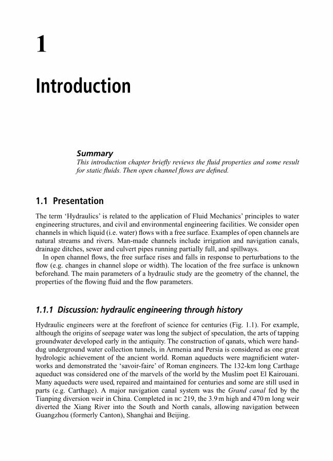
1

Introduction

SummaryThis introduction chapter briefly reviews the fluid properties and some resultfor static fluids. Then open channel flows are defined.

1.1 Presentation

The term ‘Hydraulics’ is related to the application of Fluid Mechanics’ principles to waterengineering structures, and civil and environmental engineering facilities. We consider openchannels in which liquid (i.e. water) flows with a free surface. Examples of open channels arenatural streams and rivers. Man-made channels include irrigation and navigation canals,drainage ditches, sewer and culvert pipes running partially full, and spillways.

In open channel flows, the free surface rises and falls in response to perturbations to theflow (e.g. changes in channel slope or width). The location of the free surface is unknownbeforehand. The main parameters of a hydraulic study are the geometry of the channel, theproperties of the flowing fluid and the flow parameters.

1.1.1 Discussion: hydraulic engineering through history

Hydraulic engineers were at the forefront of science for centuries (Fig. 1.1). For example,although the origins of seepage water was long the subject of speculation, the arts of tappinggroundwater developed early in the antiquity. The construction of qanats, which were hand-dug underground water collection tunnels, in Armenia and Persia is considered as one greathydrologic achievement of the ancient world. Roman aqueducts were magnificient water-works and demonstrated the ‘savoir-faire’ of Roman engineers. The 132-km long Carthageaqueduct was considered one of the marvels of the world by the Muslim poet El Kairouani.Many aqueducts were used, repaired and maintained for centuries and some are still used inparts (e.g. Carthage). A major navigation canal system was the Grand canal fed by theTianping diversion weir in China. Completed in BC 219, the 3.9 m high and 470 m long weirdiverted the Xiang River into the South and North canals, allowing navigation betweenGuangzhou (formerly Canton), Shanghai and Beijing.

The development of hydraulic engineering is closely linked to the beginnings of civil engin-eering as a separate discipline, and the foundation of the ‘Corps des Ponts et Chaussées’(Bridge and Highway Corps) in France in 1716 with the establishment of the ‘École Nationaledes Ponts et Chaussées’ (National School of Bridges and Highways) in 1747. Among thedirectors of the school were the famous hydraulicians A. Chézy (1717–1798) and G. deProny (1755–1839). Other famous professors included B.F. de Bélidor (1693–1761), J.B.C. Bélanger (1789–1874), J.A.C. Bresse (1822–1883), G.G. Coriolis (1792–1843) andL.M.H. Navier (1785–1835).

4 Introduction

(a)

(b)

Fig. 1.1 Ancient hydraulic engineering. (a) Nabataean Dam on the Mamshit stream (also called Mampsis or Kunub)on 10 May 2001 (courtesy of Dennis Murphy). Dam wall built around the end of 1st Century BC, downstream slopeof the dam wall. (b) Roman aqueduct in Fréjus, Arches de Sainte Croix, downstream of Chateau Aurélien on 14 September 2000. Looking upstream, note the slight bend in the aqueduct in the background.

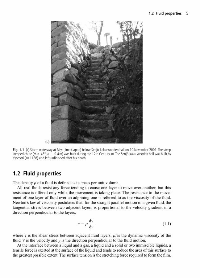
1.2 Fluid properties

The density � of a fluid is defined as its mass per unit volume.All real fluids resist any force tending to cause one layer to move over another, but this

resistance is offered only while the movement is taking place. The resistance to the move-ment of one layer of fluid over an adjoining one is referred to as the viscosity of the fluid.Newton’s law of viscosity postulates that, for the straight parallel motion of a given fluid, thetangential stress between two adjacent layers is proportional to the velocity gradient in adirection perpendicular to the layers:

(1.1)

where � is the shear stress between adjacent fluid layers, � is the dynamic viscosity of thefluid, V is the velocity and y is the direction perpendicular to the fluid motion.

At the interface between a liquid and a gas, a liquid and a solid or two immiscible liquids, atensile force is exerted at the surface of the liquid and tends to reduce the area of this surface tothe greatest possible extent. The surface tension is the stretching force required to form the film.

� � dd

V�

y

1.2 Fluid properties 5

(c)

Fig. 1.1 (c) Storm waterway at Miya-jima (Japan) below Senjò-kaku wooden hall on 19 November 2001. The steepstepped chute (� � 45°, h � 0.4 m) was built during the 12th Century AD. The Senjò-kaku wooden hall was built byKyomori (AD 1168) and left unfinished after his death.

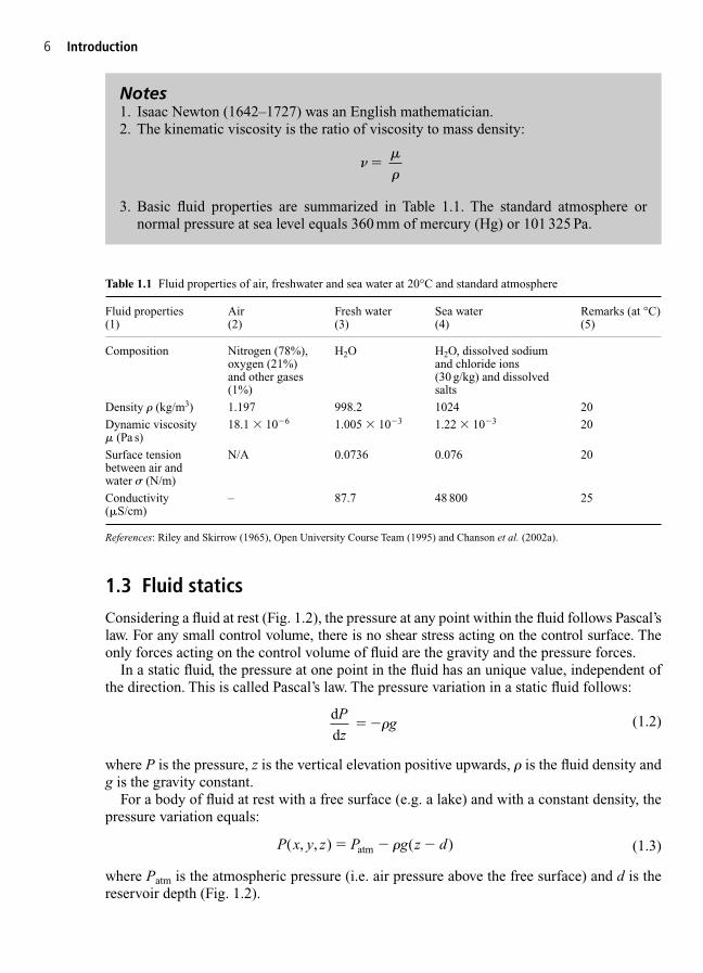
6 Introduction

1.3 Fluid statics

Considering a fluid at rest (Fig. 1.2), the pressure at any point within the fluid follows Pascal’slaw. For any small control volume, there is no shear stress acting on the control surface. Theonly forces acting on the control volume of fluid are the gravity and the pressure forces.

In a static fluid, the pressure at one point in the fluid has an unique value, independent ofthe direction. This is called Pascal’s law. The pressure variation in a static fluid follows:

(1.2)

where P is the pressure, z is the vertical elevation positive upwards, � is the fluid density andg is the gravity constant.

For a body of fluid at rest with a free surface (e.g. a lake) and with a constant density, thepressure variation equals:

(1.3)

where Patm is the atmospheric pressure (i.e. air pressure above the free surface) and d is thereservoir depth (Fig. 1.2).

P x y z P g z d( , , ) ( )atm� � ��

dd

Pz

g� ��

Table 1.1 Fluid properties of air, freshwater and sea water at 20°C and standard atmosphere

Fluid properties Air Fresh water Sea water Remarks (at °C)(1) (2) (3) (4) (5)

Composition Nitrogen (78%), H2O H2O, dissolved sodiumoxygen (21%) and chloride ions and other gases (30 g/kg) and dissolved (1%) salts

Density � (kg/m3) 1.197 998.2 1024 20

Dynamic viscosity 18.1 � 10�6 1.005 � 10�3 1.22 � 10�3 20� (Pa s)

Surface tension N/A 0.0736 0.076 20between air and water (N/m)

Conductivity – 87.7 48 800 25(�S/cm)

References: Riley and Skirrow (1965), Open University Course Team (1995) and Chanson et al. (2002a).

Notes1. Isaac Newton (1642–1727) was an English mathematician.2. The kinematic viscosity is the ratio of viscosity to mass density:

3. Basic fluid properties are summarized in Table 1.1. The standard atmosphere or normal pressure at sea level equals 360 mm of mercury (Hg) or 101 325 Pa.

��

� �

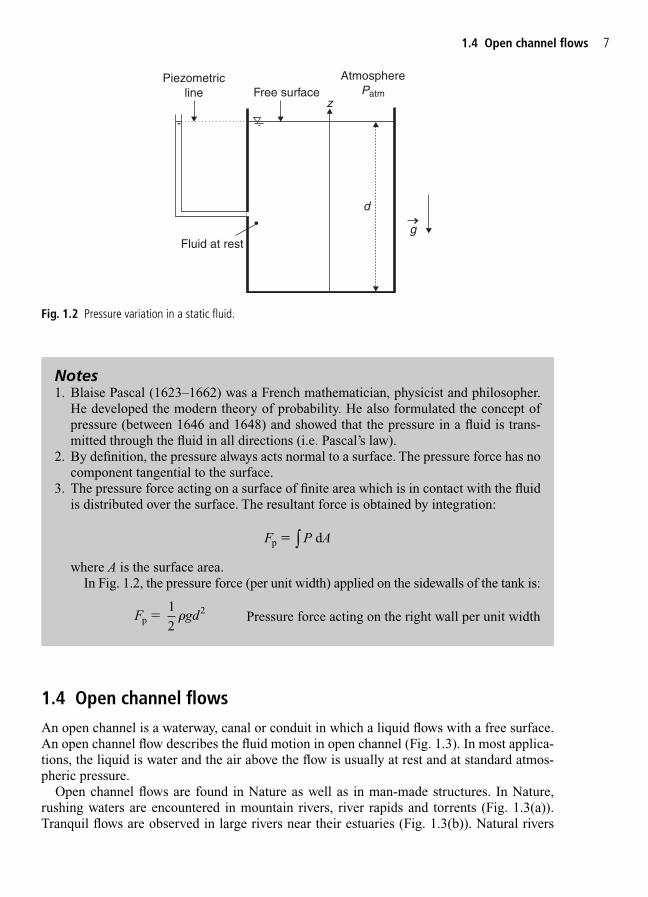
1.4 Open channel flows

An open channel is a waterway, canal or conduit in which a liquid flows with a free surface.An open channel flow describes the fluid motion in open channel (Fig. 1.3). In most applica-tions, the liquid is water and the air above the flow is usually at rest and at standard atmos-pheric pressure.

Open channel flows are found in Nature as well as in man-made structures. In Nature,rushing waters are encountered in mountain rivers, river rapids and torrents (Fig. 1.3(a)).Tranquil flows are observed in large rivers near their estuaries (Fig. 1.3(b)). Natural rivers

1.4 Open channel flows 7

z

d

Free surface

Fluid at rest

AtmospherePatm

g

Piezometricline

Fig. 1.2 Pressure variation in a static fluid.

Notes1. Blaise Pascal (1623–1662) was a French mathematician, physicist and philosopher.

He developed the modern theory of probability. He also formulated the concept ofpressure (between 1646 and 1648) and showed that the pressure in a fluid is trans-mitted through the fluid in all directions (i.e. Pascal’s law).

2. By definition, the pressure always acts normal to a surface. The pressure force has nocomponent tangential to the surface.

3. The pressure force acting on a surface of finite area which is in contact with the fluidis distributed over the surface. The resultant force is obtained by integration:

where A is the surface area.In Fig. 1.2, the pressure force (per unit width) applied on the sidewalls of the tank is:

Pressure force acting on the right wall per unit widthF gdp2

12

� �

F P Ap d� ∫

8 Introduction

(a)

(b)

Fig. 1.3 Examples of open channel flow. (a) Russel Falls in Tasmania (Australia) (courtesy of Dr R. Manasseh).(b) Eprapah Creek, Queensland (Australia) on 24 November 2003 at sunrise.

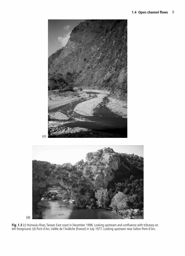
1.4 Open channel flows 9

(c)

(d)

Fig. 1.3 (c) Hsinwulu River, Taiwan East coast in December 1998. Looking upstream and confluence with tributary onleft-foreground. (d) Pont d’Arc, Vallée de l’Ardèche (France) in July 1977. Looking upstream near Vallon-Pont-d’Arc.

have the ability to scour channel beds, to carry sediment materials, and to deposit sedimentloads (Fig. 1.3(c) and (d)).

River flow rates may range from extreme values: the hydraulics of droughts and floods areboth important.

1.5 Exercises

Give the values (and units) of the specified fluid and physical properties:

(a) Density of water at atmospheric pressure and 20°C.(b) Density of air at atmospheric pressure and 20°C.(c) Dynamic viscosity of water at atmospheric pressure and 20°C.(d) Kinematic viscosity of water at atmospheric pressure and 20°C.(e) Kinematic viscosity of air at atmospheric pressure and 20°C.(f) Surface tension of air and water at atmospheric pressure and 20°C.(g) Acceleration of gravity in Brisbane.

In a static fluid, express the pressure variation with depth.

10 Introduction

2

Fundamentals of open channel flows

SummaryThe general principles of fluid mechanics are applicable to open channelflows. After a brief summary, the hydraulics of short transitions is developed,including the concept of specific energy, critical flow conditions and thehydraulic jump. Then flow resistance calculations at uniform equilibrium aredetailed and gradually varied flow (GVF) calculations are developed (i.e.backwater calculations). The application of basic principles to open channelflow situations is summarized at the end.

2.1 Presentation

An open channel is a waterway, canal or conduit in which a liquid flows with a free surface(Fig. 2.1). Classical examples include natural streams (Fig. 2.1(a)–(c)) and man-made water-ways (Fig. 2.1(d)–(f)). Figure 2.1(a)–(c) shows small and large rivers with quiet and cascadingregimes. Figure 2.1(e) shows culvert during a dry period with some students surveying thestructure. Figure 2.1(f) presents the same structure during a medium rainstorm.

Open channel flow describes the fluid motion in open channel. The free surface is at con-stant atmospheric pressure. The driving force of the fluid motion is a combination of pressure(e.g. beneath a sluice gate) and gravity (e.g. sloping channel). For a given flow rate, the pri-mary unknown is the location of the free surface which is not known beforehand. The freesurface rises and falls in response to perturbations to the flow: e.g. changes in channel eleva-tion, reduction in channel width. The main parameters of any hydraulic study are the proper-ties of the fluids (e.g. density, viscosity), the geometry of the channel (e.g. cross-sectionalshape, bed slope) and the flow properties (e.g. depth, velocity).

Basic definitionsIn an open channel, the pressure distribution is nearly always hydrostatic, unless the curva-ture of the streamlines is important (e.g. under waves). The mean total head is defined as:

(2.1)H d zV

g cos o

2

� �2

where H is the total head, d is the water depth measured normal to the bed, � is the bed slope,zo is the bed elevation, V is the depth-averaged flow velocity and g is the gravity acceleration(Fig. 2.2). In the definition of the total head, each term is analogous to a form of energy perunit mass: d cos � is the pressure head, zo is the potential head which is proportional to the

12 Fundamentals of open channel flows

(a)

(b)

Fig. 2.1 Examples of open channel flows. (a) Brisbane River at Colleges Crossing, Karana Downs, Qld (Australia) on1 September 2002 – looking upstream. (b) Rapid at Grand-Remous township on 13 July 2002, Gatineau River, Québec(Canada) – looking upstream.

potential energy per unit mass and V2/2g is the kinetic energy head. If there is no energy loss,the sum of the fluid’s potential energy, kinetic energy and pressure work is a constant and thetotal head H is a constant. Along a streamline, the energy of the flow may be re-arrangedbetween kinetic energy (i.e. velocity), potential energy (i.e. invert elevation) or pressure work(i.e. flow depth) but the sum of all terms must remain constant.

2.1 Presentation 13

(c)

(d)

Fig. 2.1 (c) Saint-Laurent River, Montréal (Canada) on 12 July 2002 – looking downstream from Vieux-Portwith Pont Jacques Cartier. (d) Escalier d’eau des jardins du Château du Touvet, 1763 (courtesy of Mr Bruno deQuinsonas) – water staircase.

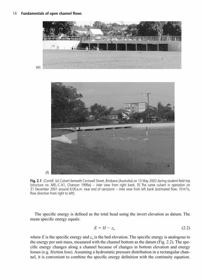
The specific energy is defined as the total head using the invert elevation as datum. Themean specific energy equals:

E � H � zo (2.2)

where E is the specific energy and zo is the bed elevation. The specific energy is analogous tothe energy per unit mass, measured with the channel bottom as the datum (Fig. 2.2). The spe-cific energy changes along a channel because of changes in bottom elevation and energylosses (e.g. friction loss). Assuming a hydrostatic pressure distribution in a rectangular chan-nel, it is convenient to combine the specific energy definition with the continuity equation.

14 Fundamentals of open channel flows

(e)

(f)

Fig. 2.1 (Contd) (e) Culvert beneath Cornwall Street, Brisbane (Australia) on 13 May 2002 during student field trip(structure no. MEL-C-X1, Chanson 1999a) – inlet view from right bank. (f) The same culvert in operation on 31 December 2001 around 6:00 a.m. near end of rainstorm – inlet view from left bank (estimated flow: 70 m3/s,flow direction from right to left).

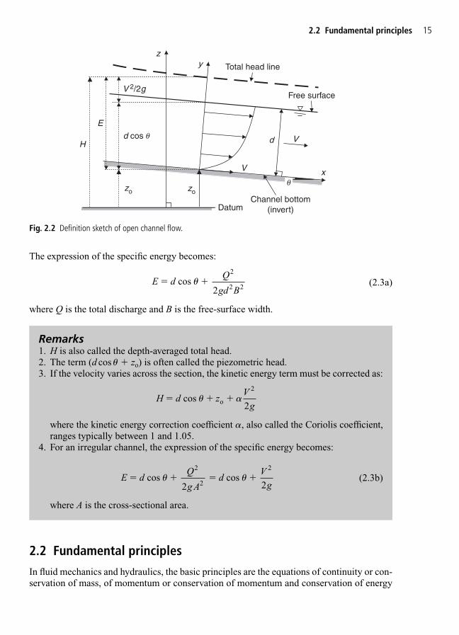
2.2 Fundamental principles

In fluid mechanics and hydraulics, the basic principles are the equations of continuity or con-servation of mass, of momentum or conservation of momentum and conservation of energy

2.2 Fundamental principles 15

Free surface

V

y

d

zo zo

x

Channel bottom(invert)

z

Total head line

Datum

V

d cos u

V 2/2g

H

E

u

Fig. 2.2 Definition sketch of open channel flow.

Remarks1. H is also called the depth-averaged total head.2. The term (d cos � zo) is often called the piezometric head.3. If the velocity varies across the section, the kinetic energy term must be corrected as:

where the kinetic energy correction coefficient �, also called the Coriolis coefficient,ranges typically between 1 and 1.05.

4. For an irregular channel, the expression of the specific energy becomes:

(2.3b)

where A is the cross-sectional area.

E dQ

g Ad

Vg

cos cos 2

2

2

� � � �2 2

H d zV

g cos o

2

� � �2

The expression of the specific energy becomes:

(2.3a)

where Q is the total discharge and B is the free-surface width.

E dQ

gd B cos

2

2 2� �

2

(Henderson 1966, Chanson 1999a). Another equation is the Bernoulli equation which may bederived from the differential form of the momentum principle. In this chapter, the simplestform of the fundamental principles is developed: i.e. for steady one-dimensional flows.Unsteady flow equations are developed in Part 3.

The law of conservation of mass, or continuity equation, states that the mass within aclosed system remains constant with time. For an incompressible fluid such as water, theinflow must equal the outflow:

Q � V1A1 � V2 A2 (2.4)

where Q is the total flow rate (i.e. volume discharge), V1 and V2 are the mean velocity acrossthe cross-sections A1 and A2 respectively, and the subscripts 1 and 2 refer to the upstream anddownstream flow cross-sections respectively.

The momentum principle states that, for a given control volume, the rate of change inmomentum flux equals the sum of the forces acting on the control volume. The rate of changein momentum flux is the sum of momentum accumulation into the control volume plus themomentum flux in minus the momentum flux out. Considering the steady overflow above abroad-crested weir placed in a horizontal, rectangular channel sketched in Fig. 2.3, the forces

16 Fundamentals of open channel flows

Free surface

Datum

H2

E2

E3

E1H1

H3

d3

d2V2V1

V1

d1

d1

dc

zo2zo1

Total head line

V /2g22

Free surface

d3

Hydrostaticpressure

distributionHydrostaticpressure

distributionFriction force

Reaction force of the weiron the flow

1

3

(a)

(b)

Fig. 2.3 Broad-crested weir overflow. (a) Definition sketch. (b) Forces applied to the control volume.

applied to the control volume delimited by the cross-sections 1 and 3 are the pressure forces act-ing on sections 1 and 3, the reaction force of the weir onto the flow, the boundary friction, theweight of water of the control volume, and the reaction force of the channel bed which opposesexactly the weight of water. The momentum equation applied in the horizontal direction yields:

(2.5)

where � is the fluid density, B is the channel width, Ffriction is the boundary friction and Fweiris the reaction force of the weir (Fig. 2.3).

The energy principle states that the net energy supplied to a system equals the energy thatleaves the system as work is done plus the increase in energy of the system which is the sumof the potential energy, kinetic energy and internal energy. In open channel hydraulics, theenergy principle is often expressed in terms of the total head:

H1 � H3 �H (2.6)

where the total head is in metres (of water) and �H is the sum of the head losses between sections 1 and 3.

� � � �QV QV gd B gd B F F3 1 friction weir � � � � �12

121

232

2.2 Fundamental principles 17

Remarks1. The momentum principle is always used for hydrodynamic force calculations:

e.g. force acting on a gate, flow resistance in uniform equilibrium flow. Other applica-tions include the hydraulic jump, positive surge and bore.

2. The total momentum flux across a section equals �VVA � �QV. The rate of change inmomentum flux is then: (�QV3 � �QV1) in a horizontal channel, as sketched in Figure 2.3.

3. For a horizontal rectangular channel with hydrostatic distribution, the pressure forceat a cross-section is:

4. The reaction force Fweir of the weir onto the fluid equals exactly the horizontal com-ponent of the resultant of the pressure forces acting on the weir.

5. If the velocity distribution is not uniform, the momentum flux terms must be cor-rected by a momentum correction coefficient �, also called Boussinesq coefficient.For the above example, it yields:

6. Further discussions on the momentum principle were developed in Henderson (1966,pp. 5–9 and 66–77) and Chanson (1999a, pp. 11–17 and 51–97).

7. In open channel flows, the friction loss �H over a distance �x along the flow direc-tion is given by the Darcy equation:

where f is the Darcy friction factor, V is the mean flow velocity and DH is thehydraulic diameter or equivalent pipe diameter.

� ��

H fx

DV

g

H

2

2

� � � � � �3 3 1 1 friction weir QV QV gd B gd B F F� � � � �12

121

232

12

2�gd B

Discussion: the Bernoulli equationThe Bernoulli equation derives from the momentum principle: i.e. the Navier–Stokes equa-tion (Liggett 1993, Chanson 1999a). Considering the flow along a streamline, assuming thatthe gravity force is independent of the time, for a frictionless and incompressible fluid, andfor a steady flow, the Navier–Stokes equation yields the differential form of the Bernoulliequation:

(2.7)

where V is the velocity, g is the gravity constant, z is the altitude, positive upwards, P is thepressure and � is the fluid density.

In an open channel, the integral form of Bernoulli equation is commonly written as:

(2.8a)

assuming a hydrostatic pressure distribution. For the smooth and short transition sketch inFig. 2.3, the above equation may be rewritten as:

H1 � H2 � H3 (2.8b)

H z dV

g cos constanto

2

� ��2

d d d 0

Pg z V V

� �

18 Fundamentals of open channel flows

8. A broad-crested weir is a flat-crested structure with a crest length large compared tothe flow thickness. When the crest is broad enough for the flow streamlines to be parallel to the crest, the pressure distribution above the crest is hydrostatic and thecritical flow depth is observed on the weir crest. Broad-crested weirs are sometimesused as critical depth meters: i.e. to measure stream discharges.

Remarks1. The Navier–Stokes equation was first derived by Navier in 1822 and Poisson in 1829

by an entirely different method. It was derived later in a manner similar by Barré deSaint-Venant in 1843 and Stokes in 1845.

2. Louis Navier (1785–1835) was a French engineer who primarily designed bridge butalso extended Euler’s equations of motion. Siméon Denis Poisson (1781–1840) wasa French mathematician and scientist. He developed the theory of elasticity, a theoryof electricity and a theory of magnetism. Adhémar Jean Claude Barré de Saint-Venant(1797–1886), French engineer, developed the equations of motion of a fluid particlein terms of the shear and normal forces exerted on it. George Gabriel Stokes (1819–1903), British mathematician and physicist, is known for his research in hydro-dynamics and a study of elasticity.

3. The Bernoulli equation is named after the Swiss mathematician Daniel Bernoulli(1700–1782) who developed the equation in his ‘Hydrodynamica, de viribus etmotibus fluidorum’ textbook (1st draft in 1733, first publication in 1738, Strasbourg).

4. For a one-dimensional flow, the Bernoulli equation differs the energy equation by theloss term only, although the Bernoulli principle derives from the momentum equation.

Applications to open channel flow situationsIn open channels, the application of the basic principles is a function of the flow situations.Basic flow situations are summarized in Table 2.1. These are discussed and developed in thefollowing paragraphs. For smooth and short transitions, the continuity and Bernoulli equa-tions form a system of two equations enabling to compute the downstream flow properties asfunctions of the upstream flow properties (e.g. Fig. 2.3). For a sudden transition from super-to subcritical flows, the continuity and momentum equations must be applied. The assump-tion of zero energy loss is untrue in a hydraulic jump. In a long prismatic channel with a constant flow rate, the flow motion reaches uniform equilibrium. That is, the flow resistanceequals exactly and opposes the gravity force component in the flow direction.

2.3 Open channel hydraulics of short, frictionless transitions

Considering a smooth, short and frictionless transition, the continuity and Bernoulli equa-tions applied to the open channel flow become:

V1A1 � V2 A2 � Q (2.9)

(2.10)z dV

gz d

Vgo 1 1 o 2 21 2

cos cos � � �12

22

2 2

2.3 Open channel hydraulics of short, frictionless transitions 19

5. The Bernoulli equation is often used for smooth, short transition: e.g. sluice gate,broad-crested weir.

6. For the broad-crested weir sketched in Fig. 2.3, the Bernoulli equation may be writtenin terms of the specific energy:

E E z z E1 2 3 ) o o2 1� � �(

Table 2.1 Applications of the basic principles to simple flow situations

Flow situation Basic principles Remarks(1) (2) (3)

Steady flowSmooth, short and frictionless Continuity Bernoulli The momentum principle may be used totransition calculate the forced exerted by the flow

onto a structure (e.g. gate, weir)

Hydraulic jump Continuity momentum The energy equation provides additionallythe rate of energy dissipation

Uniform equilibrium flow Continuity momentum Also called normal flow conditions

GVF Differential form of the Also called backwater calculationsenergy equation

Unsteady flowUnsteady GVF Differential form of the Also called Saint-Venant

continuity and momentum equations (Part 3)principles

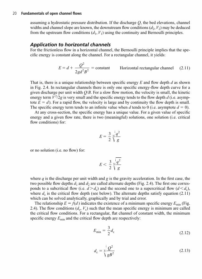
assuming a hydrostatic pressure distribution. If the discharge Q, the bed elevations, channelwidths and channel slope are known, the downstream flow conditions (d2, V2) may be deducedfrom the upstream flow conditions (d1, V1) using the continuity and Bernoulli principles.

Application to horizontal channelsFor the frictionless flow in a horizontal channel, the Bernoulli principle implies that the spe-cific energy is constant along the channel. For a rectangular channel, it yields:

Horizontal rectangular channel (2.11)

That is, there is a unique relationship between specific energy E and flow depth d as shownin Fig. 2.4. In rectangular channels there is only one specific energy-flow depth curve for agiven discharge per unit width Q/B. For a slow flow motion, the velocity is small, the kineticenergy term V 2/2g is very small and the specific energy tends to the flow depth d (i.e. asymp-tote E � d ). For a rapid flow, the velocity is large and by continuity the flow depth is small.The specific energy term tends to an infinite value when d tends to 0 (i.e. asymptote d � 0).

At any cross-section, the specific energy has a unique value. For a given value of specificenergy and a given flow rate, there is two (meaningful) solutions, one solution (i.e. criticalflow conditions) for:

or no solution (i.e. no flow) for:

where q is the discharge per unit width and g is the gravity acceleration. In the first case, thetwo possible flow depths d1 and d2 are called alternate depths (Fig. 2.4). The first one corres-ponds to a subcritical flow (i.e. d �dc) and the second one to a supercritical flow (d �dc),where dc is the critical flow depth (see below). The alternate depths satisfy equation (2.11)which can be solved analytically, graphically and by trial and error.

The relationship E � f(d ) indicates the existence of a minimum specific energy Emin (Fig.2.4). The flow conditions (dc, Vc) such that the mean specific energy is minimum are calledthe critical flow conditions. For a rectangular, flat channel of constant width, the minimumspecific energy Emin and the critical flow depth are respectively:

(2.12)

(2.13)dQ

gBc

2

23 �

E dmin c �32

Eqg

32

23�

Eqg

32

23�

E dQ

gd B constant

2

2 2� �

2

20 Fundamentals of open channel flows

2.3 Open channel hydraulics of short, frictionless transitions 21

EEmin

Critical flowconditions

Subcriticalflow

Supercriticalflow

E1 � E2

d1

d2

dc

d2

d1

d

(a)

00 2 4 6

2

4

6d /dc

E/dc

Slope 1:1

Critical flow conditions

(b)

Fig. 2.4 Relationship between specific energy and flow depth. (a) Definition sketch. (b) Dimensionless specificenergy curve for a flat rectangular channel.

Remarks1. The critical flow velocity equals in a rectangular channel.2. For a constant specific energy E, equation (2.11) is a cubic equation in terms of the

water depth d. For E � Emin, there are three solutions (e.g. Chanson 1999a, pp.143–145). One is negative and has no physical meaning.

V gdc c �

The specific energy can be rewritten in dimensionless terms as:

(2.14)

Equation (2.14) is a unique curve, valid for any discharge. It is presented in Fig. 2.4(b).

Ed

dd

ddc c

c 12

�

2

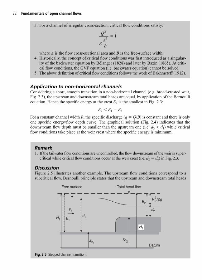
Application to non-horizontal channelsConsidering a short, smooth transition in a non-horizontal channel (e.g. broad-crested weir,Fig. 2.3), the upstream and downstream total heads are equal, by application of the Bernoulliequation. Hence the specific energy at the crest E2 is the smallest in Fig. 2.3:

E2 � E1 � E3

For a constant channel width B, the specific discharge (q � Q/B) is constant and there is onlyone specific energy/flow depth curve. The graphical solution (Fig. 2.4) indicates that thedownstream flow depth must be smaller than the upstream one (i.e. d3 � d1) while criticalflow conditions take place at the weir crest where the specific energy is minimum.

22 Fundamentals of open channel flows

3. For a channel of irregular cross-section, critical flow conditions satisfy:

where A is the flow cross-sectional area and B is the free-surface width.4. Historically, the concept of critical flow conditions was first introduced as a singular-

ity of the backwater equation by Bélanger (1828) and later by Bazin (1865). At criti-cal flow conditions, the GVF equation (i.e. backwater equation) cannot be solved.

5. The above definition of critical flow conditions follows the work of Bakhmeteff (1912).

Q

gAB

2

3 1�

Remark1. If the tailwater flow conditions are uncontrolled, the flow downstream of the weir is super-

critical while critical flow conditions occur at the weir crest (i.e. d2 � dc) in Fig. 2.3.

DiscussionFigure 2.5 illustrates another example. The upstream flow conditions correspond to asubcritical flow. Bernoulli principle states that the upstream and downstream total heads

Free surface

Datum

H2

d1E1H1

E2

d2V1

zo1zo2

Total head line

V 2 /2g2

Fig. 2.5 Stepped channel transition.

Froude numberThe Froude number is a dimensionless number proportional to the square root of the ratio ofthe inertial forces over the weight of fluid. For a horizontal rectangular channel, the Froudenumber is defined as:

Rectangular channel (2.15)

Model studies of open channel flows and hydraulic structures are performed using a Froudesimilitude. That is, the Froude number must be the same for the model and the prototype.

FrV

gd �

2.3 Open channel hydraulics of short, frictionless transitions 23

Remarks1. In horizontal, rectangular channels, the Froude number is unity at critical flow condi-

tions. It may be rewritten as:

2. For a horizontal channel of irregular cross-sectional shape, the Froude number is usually defined as:

where A is the flow cross-section and B the free-surface width. With such a definition,Fr � 1 at critical flow conditions.

3. In open channel flows, it is strongly advised to define the Froude number such asFr � 1 at critical flow conditions. That is, Fr � 1 for subcritical flow (d � dc) andFr � 1 for supercritical flow (d � dc).

FrV

gAB

�

Frdd

c�

3 2/

must be equal. Hence the downstream specific energy is the smallest. For B1 � B2, thegraphical solution (Fig. 2.4) indicates that the downstream flow depth must be smallerthan the upstream one (i.e. d2 � d1) provided that E2 � 1.5dc. This flow situation issketched in Fig. 2.5. For a supercritical upstream flow (i.e. d1 � dc), the relation wouldbe inverted: i.e. a decrease of specific energy implies an increase in flow depth.

Note that, in Fig. 2.5, there is no flow motion for E1 � (zo2� zo1

). For E1 � (zo2� zo1

)� E2 � 1.5dc, the flow rate must be less than Q: i.e. choking occurs at the step.

DiscussionThe application of the Bernoulli equation is valid only within the range of assumptions: i.e. steady frictionless flow of incompressible fluid. For short and smooth transitions theenergy losses are negligible and the Bernoulli equation may be applied successfully. If energylosses occur, they must be taken in account and the Bernoulli equation is no longer valid. For example, the Bernoulli equation is not valid at a hydraulic jump where turbulent energylosses are significant.

2.4 The hydraulic jump

In open channels, the transition from a rapid, supercritical flow to a slow, subcritical flow iscalled a hydraulic jump (Fig. 2.6). The transition occurs suddenly and it is characterized by asudden rise of the free surface, with strong energy dissipation and mixing, large-scale turbu-lence, air entrainment, waves and spray (Fig. 2.6(b) and (c)).

A hydraulic jump is a marked flow discontinuity. The momentum principle is used to evalu-ate the basic flow properties in a hydraulic jump. Considering a horizontal, rectangular openchannel of constant width B, and neglecting the shear stress at the channel bottom, the resultantof the forces acting in the x-direction are the resultant of hydrostatic pressure forces at theends of the control volume (Fig. 2.6(a)). The continuity equation and momentum equations are:

V1d1B � V2d2B (2.16)

(2.17)

where B is the channel width and Q is the total discharge (i.e. Q � VdB). It yields a relation-ship between the upstream and downstream flow depths:

(2.18)

where Fr1 is the upstream Froude number: . The depth d1 and d2 are referredto as conjugate depths or sequent depths. Using equation (2.18) the momentum equation yields:

(2.19)

where Fr2 is the downstream Froude number.

FrFr

Fr2

3/21

2

8 1

�

�1 12

3 2

/

Fr V gd1 1 1 � /

dd

Fr2

1

12

1 8 1� �12

� � �Q V V gd gd B( 2 1� � �)12

121

222

24 Fundamentals of open channel flows

Hydraulic jump

x

d1

d2

V2

V1Fp1

Fp2

zo

Ffriction

Roller

Weight force

Reactionforce

Pressureforce

(a)

Fig. 2.6 Hydraulic jump flows. (a) Definition sketch of a hydraulic jump in a horizontal channel.

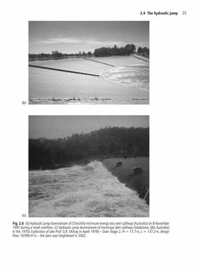
2.4 The hydraulic jump 25

(b)

(c)

Fig. 2.6 (b) Hydraulic jump downstream of Chinchilla minimum energy loss weir spillway (Australia) on 8 November1997 during a small overflow. (c) Hydraulic jump downstream of Awoonga dam spillway (Gladstone, Qld, Australia)in the 1970s (collection of late Prof. G.R. McKay in Apelt 1978) – Dam Stage 2: H � 17.7 m, L � 137.2 m, designflow: 16 990 m3/s – the dam was heightened in 2002.

The energy equation gives the total head loss:

(2.20)� ��

Hd d

d d

( 2 1

1 2

)3

4

26 Fundamentals of open channel flows

Remarks1. An open channel flow can change from subcritical to supercritical in a relatively

‘low-loss’ manner at gates and weirs. In these cases the flow regime evolves fromsubcritical to supercritical with the occurrence of critical flow conditions associatedwith relatively small energy loss (e.g. broad-crested weir, sluice gate). The transitionfrom supercritical to subcritical flow is, on the other hand, characterized by a strongdissipative mechanism.

2. In a hydraulic jump, the upstream flow conditions are supercritical: i.e. Fr1 � 1 inequations (2.18)–(2.20).

3. Hydraulic jumps are strong energy dissipators. Hydraulic jump stilling basin arecommonly designed downstream of dam spillways to dissipate the kinetic energy ofthe flow. For example, Fig. 2.6(b) shows a hydraulic jump downstream of a weir dur-ing a small overflow. Figure 2.6(c) presents a hydraulic jump downstream of a damspillway during a medium flood.

4. Hydraulic jumps may be characterized by strong air entrainment (Fig. 2.6). Air is trapped at the impingement of the supercritical flow into the roller (see Chapter 17).

5. Experimental observations highlighted different types of hydraulic jumps, dependingupon the upstream Froude number Fr1 and inflow conditions (e.g. Chow 1973, p. 395;Chanson 1997, pp. 73–92; Chanson 1999a, pp. 57–64).

2.5 Open channel flow in long channels

2.5.1 Presentation

In open channel flows, flow resistance can be neglected over a short transition as a firstapproximation. But this assumption is invalid for long channels (Fig. 2.7). Considering awater supply canal extending over several kilometres, the boundary shear opposes the fluidmotion and retards the flow. The flow resistance and gravity effects are of the same order ofmagnitude. In fact, the friction force equals and opposes exactly the weight force componentin the flow direction at uniform equilibrium (i.e. normal flow conditions) (Fig. 2.8). The lawsof flow resistance in open channels are basically the same as those in closed pipes, although,in open channel, the calculation of boundary shear stress is complicated by the existence ofthe free surface and the wide variety of possible cross-sectional shapes (Henderson 1966,Chanson 1999a). Another difference is the propulsive force. In open channel flows, the fluidis propelled by the weight of the flowing water resolved down a slope, whereas, in closedpipes, the flow is driven by a pressure gradient along the pipe.

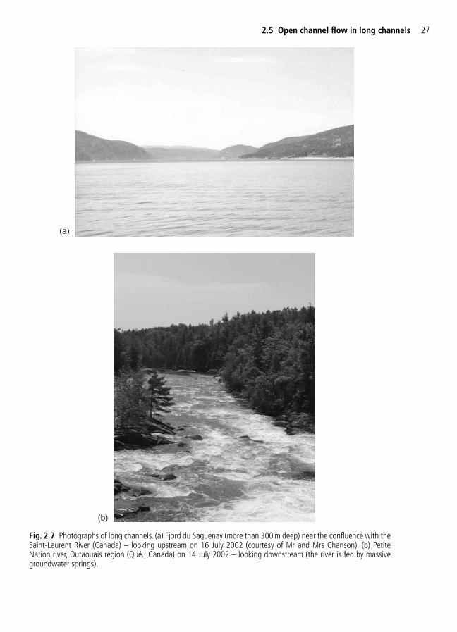
2.5 Open channel flow in long channels 27

(a)

(b)

Fig. 2.7 Photographs of long channels. (a) Fjord du Saguenay (more than 300 m deep) near the confluence with theSaint-Laurent River (Canada) – looking upstream on 16 July 2002 (courtesy of Mr and Mrs Chanson). (b) PetiteNation river, Outaouais region (Qué., Canada) on 14 July 2002 – looking downstream (the river is fed by massivegroundwater springs).

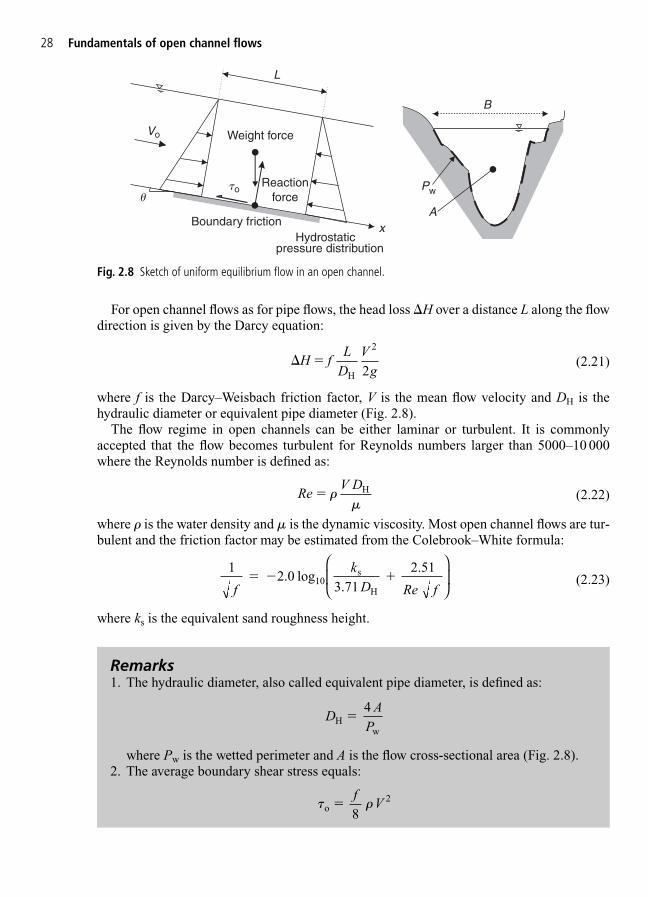
For open channel flows as for pipe flows, the head loss �H over a distance L along the flowdirection is given by the Darcy equation:

(2.21)

where f is the Darcy–Weisbach friction factor, V is the mean flow velocity and DH is thehydraulic diameter or equivalent pipe diameter (Fig. 2.8).

The flow regime in open channels can be either laminar or turbulent. It is commonlyaccepted that the flow becomes turbulent for Reynolds numbers larger than 5000–10 000where the Reynolds number is defined as:

(2.22)

where � is the water density and � is the dynamic viscosity. Most open channel flows are tur-bulent and the friction factor may be estimated from the Colebrook–White formula:

(2.23)

where ks is the equivalent sand roughness height.

1 2 51

f

kD Re f

2.0 log3.71

10s

H

� � .

ReV D

H� ��

� �H fL

DV

g

H

2

2

28 Fundamentals of open channel flows

Remarks1. The hydraulic diameter, also called equivalent pipe diameter, is defined as:

where Pw is the wetted perimeter and A is the flow cross-sectional area (Fig. 2.8).2. The average boundary shear stress equals:

� �o2

8�

fV

DA

PHw

4

�

x

Weight force

L

Boundary friction

tou

Reactionforce

Hydrostaticpressure distribution

Vo

B

A

Pw

Fig. 2.8 Sketch of uniform equilibrium flow in an open channel.

2.5.2 Uniform equilibrium flows

In steady open channel flows, a fundamental problem is determining the relation between thewater depth, the flow velocity, the channel slope and the channel geometry. Considering astraight, prismatic channel with a constant discharge, uniform equilibrium is achieved whenthe flow properties (d, V ) become independent of time and of position along the flow direc-tion. The momentum equation applied in the flow direction states the exact balance betweenthe shear forces and the gravity force component in the flow direction (Fig. 2.8). The momen-tum principle yields:

�oPwL � �gAL sin � (2.24a)

where �o is the bottom shear stress, Pw is the wetted perimeter, L is the length of the controlvolume, A is the cross-sectional area and � is the channel slope. Replacing the bottom shearstress by its expression, the momentum equation for uniform equilibrium flows becomes:

(2.24b)

where Vo is the uniform equilibrium flow velocity and (DH)o is the hydraulic diameter of uni-form equilibrium flows.

Vgf

Do

H o (

sin�8

4)

�

2.5 Open channel flow in long channels 29

3. The Colebrook–White formula is valid only in turbulent flows. In laminar flows, theDarcy friction factor equals:

Laminar flows

4. Equation (2.23) is non-linear. The Darcy–Weisbach friction factor f appears on bothsides. The Colebrook–White formula must be solved by iterations using a graphicalmethod (e.g. Moody diagram) or by trial and error.

5. Typical equivalent roughness heights are listed below:

ks (mm) Material

0.01–0.02 PVC (plastic)0.3–3 Concrete3–10 Untreated shotcrete0.6–2 Planed wood5–10 Rubble masonry

f Re

� 64

Remarks1. Uniform equilibrium flow conditions are also called normal flow conditions.2. The momentum equation for steady uniform open channel flow is rewritten usually as:

S Sf o �

2.5.3 GVF calculations

In most practical cases, the cross-section, depth and velocity in a channel vary in the flowdirection and uniform flow conditions are not often reached. Figure 2.7 illustrates examplesof longitudinal free-surface profiles in response to upstream and downstream controls. InFig. 2.7(a), the river flow is controlled by the downstream flow conditions: i.e. the tides in theBay and the flow conditions in the Saint-Laurent river. Figure 2.7(b) shows a supercriticalflow that is controlled by the upstream flow conditions.

30 Fundamentals of open channel flows

where Sf is called the friction slope and So is the channel slope defined as:

where H is the mean total head and zo is the bed elevation. The definitions of the fric-tion and bottom slopes are general and applied to both uniform equilibrium and GVF.

3. The flow resistance is sometimes expressed in terms of the Chézy equation:

where CChézy is the Chézy coefficient (unit: m1/2/s). The Chézy equation was firstintroduced as an empirical correlation. The Chézy coefficient ranges typically from30 m1/2/s (small rough channel) up to 90 m1/2/s (large smooth channel).

4. An empirical formulation, called the Gauckler–Manning formula, was developed forturbulent flows in rough channels. The Gauckler–Manning formula is:

where nManning is the Gauckler–Manning coefficient (unit: s/m1/3). The Gauckler–Manning coefficient is an empirical coefficient, found to be a characteristic of thesurface roughness primarily. Typical values of nManning (in SI unit) are:

nManning Material

0.012 Finished concrete0.014 Unfinished concrete0.029 Gravel0.05 Flood plain (light brush)0.15 Flood plain (trees)

Vn

D

1

Manning

H�4

2 3

/

sin�

V CD

4

sinChézyH� �

Szxoo sin� � �

∂∂

�

SHx gDf

o

H

4

� � �∂∂

�

�

Considering a steady open channel flow, the differential form of the energy equation written in terms of mean total head is:

(2.25a)

where x is the distance along the channel bed, f is the Darcy friction factor, DH is thehydraulic diameter, V is the mean flow velocity (i.e. V � Q/A). Equation (2.25) is called theGVF equation and it is usually rewritten as:

(2.25b)

where Sf is the friction slope.The GVF equation was first developed by J.B. Bélanger (Bélanger 1828). It is a one-

dimensional model of GVF, steady flows in open channel. It may be applied to natural and artificial channels but it is important to know the limitations. GVF calculations are devel-oped assuming a steady, non-uniform equilibrium flow, that the flow is GVF, and that the flowresistance may be estimated as in uniform equilibrium flows. That is, they do not apply touniform equilibrium flows, nor to unsteady flows nor to rapidly varied flows (RVF, e.g. thehydraulic jump).

Integration of the GVF equationTo solve the backwater equation, it is essential to determine correctly the boundary conditions.That is, the flow conditions upstream, downstream and along the channel reach. In practice,the boundary conditions are control devices (e.g. sluice gate, weir, reservoir) that imposeflow conditions for the depth, the discharge or a relationship between the discharge and thedepth, and geometric characteristics (e.g. bed elevation, channel width). Equation (2.25) is anon-linear equation which usually cannot be solved analytically, but it can be integratednumerically. One of the most common integration methods is the standard step method,developed herein and used by several numerical models.

∂∂Hx

S f� �

∂∂Hx

fD

Vg

H

2

� �1

2

2.5 Open channel flow in long channels 31

Remarks1. The GVF equation is also called the backwater equation.2. Backwater calculations may be applied to one-dimensional, steady flows. They do

not apply to hydraulic jumps nor to any RVF situation. Further there is a singularity at critical flow conditions. In fact, the concept of critical flow conditions was firstdeveloped by Bélanger (1828) as the location where d � Q2/gA2 for a flat channel. Itwas associated with the idea of minimum specific energy by Bakhmeteff (1912). BothBélanger and Bakhmeteff developed the concept of critical flow in relation with thesingularity of the backwater equation for d � Q2/gA2 (i.e. critical flow conditions).

3. Backwater computations must start from a location where the flow conditions (d, V )are known. The results are very sensitive to the flow resistance estimate (e.g. Henderson1966, Chanson 1999a).

Considering the GVF sketched in Fig. 2.9, the backwater equation is integrated betweentwo cross-sections denoted {i} and {i 1}. It yields:

(2.26a)

where the subscripts i and i 1 refer to stations {i} and {i 1} respectively. If the flow con-ditions at cross-section {i} are known, the total head at the cross-section {i 1} equals:

(2.26b)H H S S x xi i i ii i � �1 1�

12

( ( f f1) )

H Hx x

S Si i

i ii i

�

��

1

11

12

( f f� )

32 Fundamentals of open channel flows

Total headline

xu

V

Datum

z

di

Hi

Vi /2g

Vi1/2g2

Hi1

zoi1

zoi

di1

Hi � Hi1

{i }

{i1}

2

Fig. 2.9 Definition sketch of GVF calculations.

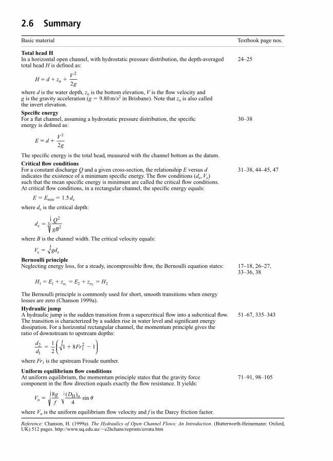
2.6 Summary

Basic material Textbook page nos.

Total head HIn a horizontal open channel, with hydrostatic pressure distribution, the depth-averaged 24–25total head H is defined as:

where d is the water depth, zo is the bottom elevation, V is the flow velocity and g is the gravity acceleration (g � 9.80 m/s2 in Brisbane). Note that zo is also called the invert elevation.

Specific energyFor a flat channel, assuming a hydrostatic pressure distribution, the specific 30–38energy is defined as:

The specific energy is the total head, measured with the channel bottom as the datum.

Critical flow conditionsFor a constant discharge Q and a given cross-section, the relationship E versus d 31–38, 44–45, 47indicates the existence of a minimum specific energy. The flow conditions (dc, Vc) such that the mean specific energy is minimum are called the critical flow conditions.At critical flow conditions, in a rectangular channel, the specific energy equals:

E � Emin � 1.5 dc

where dc is the critical depth:

where B is the channel width. The critical velocity equals:

Bernoulli principleNeglecting energy loss, for a steady, incompressible flow, the Bernoulli equation states: 17–18, 26–27,

33–36, 38

The Bernoulli principle is commonly used for short, smooth transitions when energy losses are zero (Chanson 1999a).

Hydraulic jumpA hydraulic jump is the sudden transition from a supercritical flow into a subcritical flow. 51–67, 335–343The transition is characterized by a sudden rise in water level and significant energy dissipation. For a horizontal rectangular channel, the momentum principle gives the ratio of downstream to upstream depths:

where Fr1 is the upstream Froude number.

Uniform equilibrium flow conditionsAt uniform equilibrium, the momentum principle states that the gravity force 71–91, 98–105component in the flow direction equals exactly the flow resistance. It yields:

where Vo is the uniform equilibrium flow velocity and f is the Darcy friction factor.

Vg

f

Do

H o 8 (

sin�)

4�

d

dFr2

1

12

1 8 1� �12

H E z E z H1 1 2 2 o o1 2� � �

V gdc c �

dQ

gBc

2

23 �

E dV

g

2

� 2

H d zV

g o

2�

2

Reference: Chanson, H. (1999a). The Hydraulics of Open Channel Flows: An Introduction. (Butterworth-Heinemann: Oxford,UK) 512 pages. http://www.uq.edu.au/�e2hchans/reprints/errata.htm

2.7 Exercises

1. Considering a vertical sluice gate in a horizontal smooth rectangular channel, theupstream and downstream water depths are respectively 5.1 and 0.45 m. The upstream flowvelocity is 0.5 m/s and the channel width is 27 m. Calculate the downstream flow depthand the force acting on the sluice.

2. Considering a broad-crested weir, draw a sketch of the weir. What is the main purpose ofa broad-crested weir? A broad-crested weir is installed in a horizontal and smooth channelof rectangular cross-section. The channel width is 17 m. The bottom of the weir is 2.15 mabove the channel bed. The water discharge is 24 m3/s. Compute the depth of flowupstream of the weir, above the sill of the weir and downstream of the weir (in absence ofdownstream control), assuming that critical flow conditions take place at the weir crest.Assume a frictionless flow.

3. A hydraulic jump flow takes place in a horizontal rectangular channel. The downstreamflow conditions are: d � 5.1 m, q � 14 m2/s. Calculate the upstream flow depth andFroude number, as well as the head loss in the jump.

4. A rectangular (14 m width) concrete channel carries a discharge of 10 m3/s. The longitu-dinal bed slope is 2 m/km. (a) What is the normal depth at uniform equilibrium? (b) Atuniform equilibrium what is the average boundary shear stress? (c) At normal flow condi-tions, is the flow supercritical, supercritical or critical? Would you characterize the channelas mild, critical or steep? For man-made channels, perform flow resistance calculationsbased upon the Darcy–Weisbach friction factor.

5. At uniform equilibrium, water flows in a trapezoidal grass waterway (bottom width: 2 m,sidewall slope: 1V:3H), the flow depth is 1.1 m and the longitudinal bed slope is21.3 m/km. Assume a Gauckler–Manning coefficient of 0.045 s/m1/3. Calculate: (a) dis-charge, (b) critical depth, (c) Froude number, (d) Reynolds number and (e) Chézy coeffi-cient. The fluid is water at 20°C.

6. An artificial canal carries a discharge of 12 m3/s. The channel cross-section is rectangular(9 m bottom width, 1V:2H sideslopes). The longitudinal bed slope is 7.5 m/km. The channelbottom and sidewall consist of a mixture of sands (ks � 0.9 mm). (a) What is the normaldepth at uniform equilibrium? (b) At uniform equilibrium what is the average boundaryshear stress and the shear velocity?

A gauging station is set at a bridge crossing the waterway. The observed flow depth, at the gauging station, is 2.5 m. (c) Compute the flow velocity at the gauging station. (d) Calculate the Darcy friction factor (at the gauging station). (e) What is the boundaryshear stress (at the gauging station)? (f) How would you describe the flow at the gaugingstation? (g) At the gauging station, from where is the flow controlled? Why?

34 Fundamentals of open channel flows

PART 2Turbulent Mixing and

Dispersion in Rivers andEstuaries: An Introduction

Aichi Forest Park, Japan (photograph by H. Chanson, March 1999).

Mixing and dispersion of matter in natural rivers is of considerable importance. In somecases, the release of matter into a natural system causes significant harm to the local envir-onment and it is essential to predict accurately the dispersion and mixing in the stream, andthe extent of the impact, despite the complexity of the natural system. There are severalexcellent publications covering aspects of river mixing. For example, Fischer et al. (1979)and Rutherford (1994) provide comprehensive reviews of mixing theory, and they detail howto solve particular mixing problems. This section is an attempt to draw together the importantelements from these and other important works, together with the writer’s experience in lec-turing open channel hydraulics, mixing in rivers and environmental fluid mechanics. The lec-ture material is aimed to undergraduate students who have a solid background in fluidmechanics and hydraulics. At the end of this section, the reader will have gained some basicunderstanding in turbulent mixing and dispersion in rivers, as well as a series of pre-designtools to estimate contaminant dispersion in river systems.

Internet resourcesInternet resources of relevance include:

Biography of Hugo B. Fischer http://www.oac.cdlib.org/dynaweb/ead/berkeley/wrca/fischerh/

Mixing and dispersion in riversRivers seen from space http://www.athenapub.com/rivers1.htmAerial photographs of rivers ftp://geology.wisc.edu/pub/air

Mixing and dispersion in estuariesUSACE inlets online http://www.oceanscience.net/inletsonline/Estuaries in South Africa http://www.upe.ac.za/cerm/Whirlpools http://www.uq.edu.au/�e2hchans/whirlpl.html

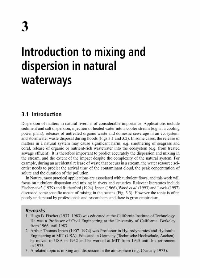
3

Introduction to mixing and dispersion in natural waterways

3.1 Introduction

Dispersion of matters in natural rivers is of considerable importance. Applications includesediment and salt dispersion, injection of heated water into a cooler stream (e.g. at a coolingpower plant), releases of untreated organic waste and domestic sewerage in an ecosystem,and stormwater waste disposal during floods (Figs 3.1 and 3.2). In some cases, the release ofmatters in a natural system may cause significant harm: e.g. smothering of seagrass andcoral, release of organic or nutrient-rich wastewater into the ecosystem (e.g. from treatedsewage effluent). It is therefore important to predict accurately the dispersion and mixing inthe stream, and the extent of the impact despite the complexity of the natural system. Forexample, during an accidental release of waste that occurs in a stream, the water resource sci-entist needs to predict the arrival time of the contaminant cloud, the peak concentration ofsolute and the duration of the pollution.

In Nature, most practical applications are associated with turbulent flows, and this work willfocus on turbulent dispersion and mixing in rivers and estuaries. Relevant literatures includeFischer et al. (1979) and Rutherford (1994). Ippen (1966), Wood et al. (1993) and Lewis (1997)discussed some specific aspect of mixing in the oceans (Fig. 3.3). However the topic is oftenpoorly understood by professionals and researchers, and there is great empiricism.

Remarks1. Hugo B. Fischer (1937–1983) was educated at the California Institute of Technology.

He was a Professor of Civil Engineering at the University of California, Berkeleyfrom 1966 until 1983.

2. Arthur Thomas Ippen (1907–1974) was Professor in Hydrodynamics and HydraulicEngineering at MIT (USA). Educated in Germany (Technische Hochschule, Aachen),he moved to USA in 1932 and he worked at MIT from 1945 until his retirement in 1973.

3. A related topic is mixing and dispersion in the atmosphere (e.g. Csanady 1973).

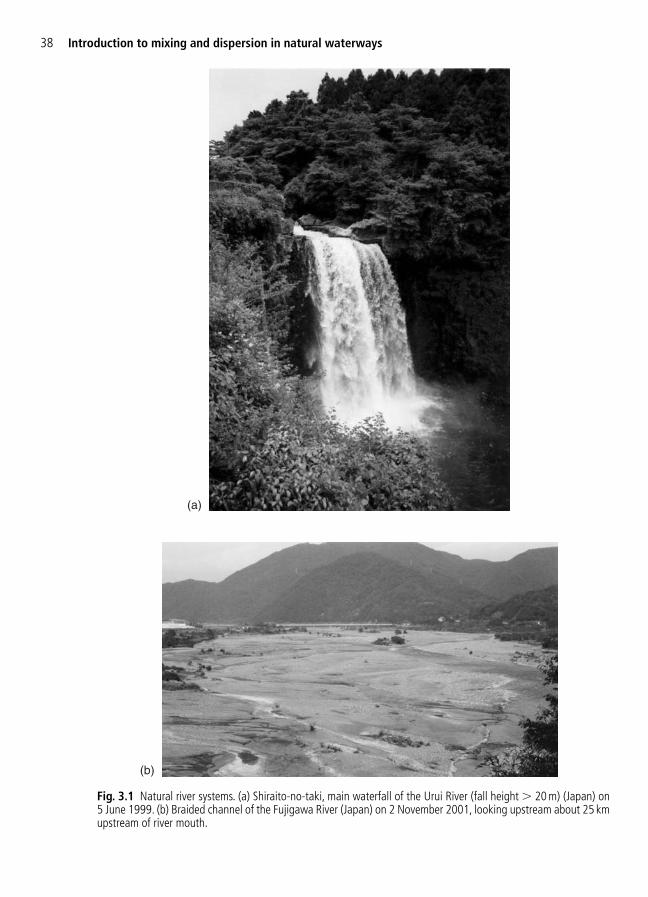
38 Introduction to mixing and dispersion in natural waterways

(a)

(b)

Fig. 3.1 Natural river systems. (a) Shiraito-no-taki, main waterfall of the Urui River (fall height � 20 m) (Japan) on5 June 1999. (b) Braided channel of the Fujigawa River (Japan) on 2 November 2001, looking upstream about 25 kmupstream of river mouth.

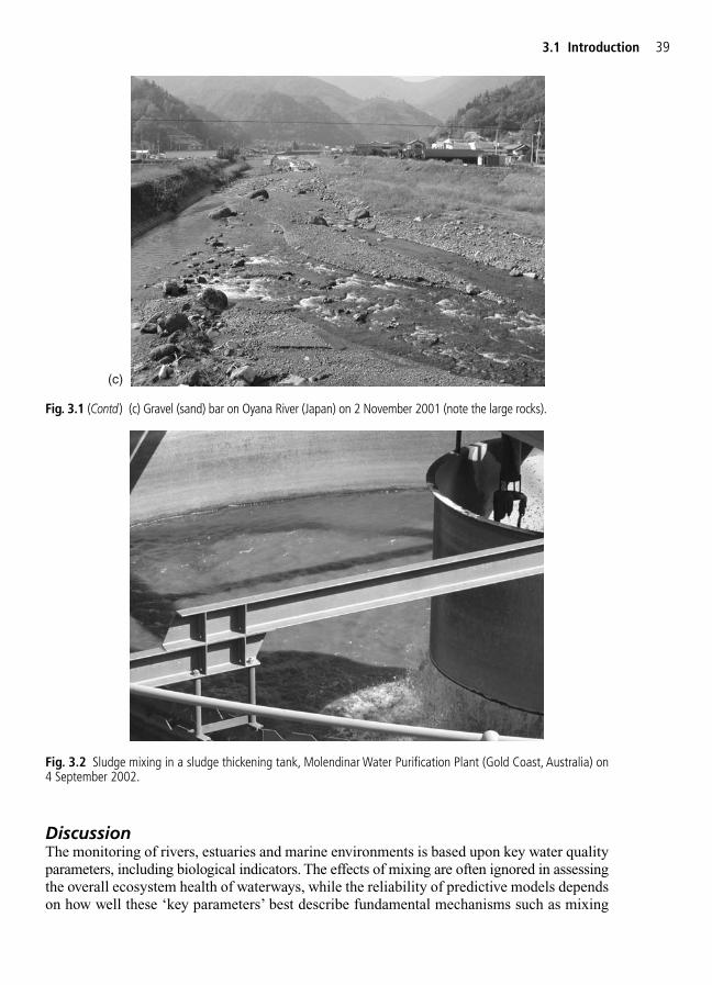
DiscussionThe monitoring of rivers, estuaries and marine environments is based upon key water qualityparameters, including biological indicators. The effects of mixing are often ignored in assessingthe overall ecosystem health of waterways, while the reliability of predictive models dependson how well these ‘key parameters’ best describe fundamental mechanisms such as mixing

3.1 Introduction 39

(c)

Fig. 3.1 (Contd) (c) Gravel (sand) bar on Oyana River (Japan) on 2 November 2001 (note the large rocks).

Fig. 3.2 Sludge mixing in a sludge thickening tank, Molendinar Water Purification Plant (Gold Coast, Australia) on4 September 2002.

and dispersion. Predictions of contaminant dispersion in creeks and streams are almostalways based upon empirical mixing and dispersion coefficients (Chapters 7–10). Thesecoefficients are highly sensitive to the natural system and flow conditions, and must be meas-ured in situ. Experimental findings are however accurate only ‘within a factor of 4’ (at best!),and they can rarely be applied to another system (Fischer et al. 1979, Rutherford 1994).While there has been considerable research on pollutant dispersion in individual river catch-ments, little systematic research has been done on the turbulent mixing and dispersion incomplete riverine and estuarine systems.

It is fundamental to comprehend that analytical and numerical models must be calibratedwith basic field measurements, and that they must be validated with other independent fieldtests.

3.2 Laminar and turbulent flows

Considering a particular situation (e.g. a pipe flow, Fig. 3.4), a low-velocity flow motion ischaracterized by fluid particles moving along smooth paths in laminas or layers, with onelayer gliding smoothly over an adjacent layer: i.e. the laminar flow regime.

With increasing flow velocity, there is a critical velocity above which the flow motionbecomes characterized by an unpredictable behaviour, strong mixing properties and a broadspectrum of length scales: i.e. a turbulent flow regime. This is illustrated in Fig. 3.4 showinga modified Reynolds experiment1 in the Hydraulics/Fluid Mechanics Laboratory at the

40 Introduction to mixing and dispersion in natural waterways

Fig. 3.3 Plume of the Var River (top left) entering the Mediterranean Sea at Nice airport (courtesy of Prof.D.H. Peregrine). Picture taken from airplane on 30 March 2001 near full moon. The Var River may carry a lot of bauxite sediments during flood and snow melt periods.

1 In his original experiment, Osborne Reynolds used a horizontal pipe.

University of Queensland. In turbulent flows the fluid particles move in very irregular paths,causing an exchange of momentum from one portion of the fluid to another. Turbulent flowshave great mixing potential and involve a wide range of eddy length scales. In naturalstreams, the flow is turbulent and strong turbulent mixing occurs.

In pipes, laminar flows are observed for Reynolds number �1000–3000, where theReynolds number is defined as Re � (�VDH)/�, where � and � are the fluid density anddynamic viscosity respectively, V is the flow velocity and DH is the hydraulic diameter orequivalent pipe diameter. Turbulent flows occur for Reynolds numbers �5000–10 000typically.

3.2 Laminar and turbulent flows 41

Dye

Dyeinjection

Laminar flow(a)

Fig. 3.4 A modified Reynolds experiment illustrating laminar and turbulent flows down a circular pipe.(a) Laminar flow (Re � 370, D � 0.0127 m on the right photograph). Note the lamina of green dye in the middleof the pipe.

Shear stressThe term shear flow characterizes a flow with a velocity gradient in a direction normal to themean flow direction: e.g. a boundary layer flow along a flat plate. In a shear flow, momentum

42 Introduction to mixing and dispersion in natural waterways

Dyeinjection

Turbulent flow(b)

Fig. 3.4 (Contd) (b) Turbulent flow (Re � 3600, D � 0.0127 m on the right photograph). High-speed photograph(1/1000 shutter speed) showing the rapid dye mixing downstream of the injection point.

Remarks1. The Reynolds number Re characterizes the ratio of inertial force to viscous force.2. Osborne Reynolds (1842–1912) was a British physicist and mathematician who

expressed first the Reynolds number (Reynolds 1883) and later the Reynolds stress orturbulent shear stress.

3. The hydraulic diameter is defined as:

where A is the flow cross-sectional area and Pw is the wetted perimeter. DH is alsocalled the equivalent pipe diameter. For a circular pipe, DH � D where D is theinternal pipe diameter.

DA

PHw

4�

(i.e. momentum per unit volume � �V) is transferred from the region of high velocity to thatof low velocity. The fluid tends to resist the shear associated with the transfer of momentum.The shear stress is proportional to the rate of transfer of momentum.

In laminar flows,2 the Newton’s law of viscosity relates the shear stress to the rate of angulardeformation:

(3.1)

where � is the shear stress, � is the dynamic viscosity of the flowing fluid, V is the velocityand y is the direction normal to the flow direction. For larger shear stresses, the fluid cannotsustain the viscous shear stress and turbulence spots develop. After apparition of turbulencespots, the turbulence expands rapidly to the entire shear flow. The apparent shear stress in turbulent flow is expressed as:

(3.2a)

where � is the kinematic viscosity (i.e. � � ���) and �T is called the ‘eddy viscosity’ ormomentum exchange coefficient in turbulent flow. The momentum exchange coefficient �T isa factor depending upon the flow motion. Practically, �T �� � in turbulent flows and equation(3.2a) becomes:

(3.2b)� � TV

� �∂∂y

� � TV

� ( )� �∂∂y

� � V

�∂∂y

3.2 Laminar and turbulent flows 43

2 That is, for a Reynolds number �1000–3000.

Remarks1. The ‘eddy viscosity’ concept was first introduced by the Frenchman J.V. Boussinesq

(1877, 1896).2. Joseph Valentin Boussinesq (1842–1929) was a French hydrodynamicist and

Professor at the Sorbonne University (Paris). His treatise ‘Essai sur la théorie deseaux courantes’ (1877) remains an outstanding contribution in hydraulics literature.

3. In the mixing length theory, the momentum exchange coefficient �T is defined as:

(3.3)

where l is the mixing length.4. The mixing length theory is a turbulence theory developed by L. Prandtl (1925). He

assumed that the mixing length l is the characteristic distance travelled by a particleof fluid before its momentum is changed by the new environment.

5. Ludwig Prandtl (1875–1953) was a German physicist and aerodynamicist who intro-duced the concept of boundary layer (Prandtl 1904). He was a Professor at theUniversity of Göttingen.

�T2

V� l

y∂∂

3.3 Basic definitions

The mass flow rate (or mass discharge) is the mass flux per unit time (unit: kg/s).The volume flow rate (or volume discharge) is the volume flux per unit time (unit: m3/s).The concentration of a contaminant Cm is defined as the mass of contaminant per unit volume(unit: kg/m3).The volume fraction is defined as the volume of tracers per unit volume (unit: dimensionless).The dilution is defined as the inverse of the volume fraction:

The density of contaminated water equals � ��, where � is the water density (unit: kg/m3).��/� is typically �3%.3 Although such changes in fluid density has little effect on fluidacceleration, they do affect buoyant discharges and the stability of density-stratified waterbodies (e.g. lakes, oceans).The buoyancy per unit mass, or modified gravitational acceleration, is defined as:

where g is the gravity acceleration.Density stratification in large water bodies (lakes, oceans) is almost often stable. It is describedby the vertical density profile �(z), where z is the vertical coordinate positive upwards.Dimensional analysis shows that a relevant dimensionless number4 is the Richardson numberdefined as:

where the sign minus is used for convenience to make Ri positive as the elevation z is posi-tive upwards.The diffusion coefficient (or diffusivity) is the quantity of a chemical that, in diffusing fromone region to another, passes through each unit of cross-section per unit of time when the vol-ume concentration is unity. The units of the diffusion coefficient are m2/s.

Rig z

z

V

2�

�

�

�∂∂

∂∂

g g� ��

�

�

Dilution 1

Volume fraction�

44 Introduction to mixing and dispersion in natural waterways

3 For analyses of shallow waters (streams, estuaries, nearshore ocean waters), it is usually necessary to work with adensity accuracy �� � 1 � 10�4kg/m3 while a density accuracy of �� � 1 � 10�6 to 1 � 10�5kg/m3 is requiredfor analyses of mixing in deep lakes, reservoirs and oceans (Fischer et al. 1979).4 Used for similitude and physical modelling.

Remarks1. The mass concentration of a substance is expressed in mass of dissolved chemical per

unit volume or kg/m3. Another unit is the parts per million (ppm). The conversion is:1 ppm � 1 mg/L.

2. The buoyancy force is a vertical force caused by pressure differences between theupper and lower surfaces of a submerged object. Calculations of the buoyancy forceexerted on a submerged air bubble are developed in Appendix A (Section 3.5).

3.4 Structure of the section

This section is an attempt to draw together the important elements from important relevantworks, together with the writer’s experience in lecturing open channel hydraulics, mixing inrivers and environmental fluid mechanics. The material presents the basic concepts of mix-ing and dispersion in rivers. It is aimed to undergraduate students who have a solid back-ground in fluid mechanics and hydraulics. At the end of the course, the reader will havegained some basic understanding in turbulent mixing and dispersion in rivers, as well as aseries of pre-design tools to estimate contaminant dispersion in river systems.

A brief summary of turbulent flows follows (Chapter 4) this chapter. The next two chap-ters (Chapters 5 and 6) present the fundamental principle of molecular diffusion and advec-tion. The results are extended to turbulent advective diffusion in channels: transverse mixing(Chapter 7) and longitudinal dispersion (Chapter 8). While Taylor’s theory, presented inChapter 8, is a simple prediction tool, dispersion in natural river systems is further complicatedby the existence of dead zones and some possible contaminant reactions. These issues aredeveloped in Chapter 9. Mixing and dispersion in estuarine zones are introduced in Chapter 10.

At the beginning of the book, the reader will find the list of symbols and a glossary of tech-nical terms and names. After the conclusion, a detailed list of references is presented.

3.4 Structure of the section 45

3. There are several definitions of the Richardson number. The above is sometimescalled the local gradient Richardson number. The Richardson number was namedafter Lewis Fry Richardson (1881–1953), a British meteorologist who took interest inthe dispersion of smoke from shell explosion during the World War I.

4. Basic fluid properties at standard atmopshere and 20°C are summarized in Table 1.1(Chapter 1). Variations of freshwater properties with temperature are given inAppendix B (Section 3.6).

RemarksIt is worth noting the number of significant contributions by Australasian academics andscientists to the field of environmental open channel flows, and mixing and dispersion inriverine, estuarine and coastal systems. Among them, J.C. Rutherford, National Instituteof Water and Atmospheric Research, Hamilton (NZ) (Rutherford 1994); Prof. Ian R.Wood, Emeritus Professor, Department of Civil Engineering, University of Canterbury,Christchurch (NZ) (Wood et al. 1993); Late Professor David L. Wilkinson (1944–1998),Department of Civil Engineering, University of Canterbury, Christchurch (NZ) and for-merly Department of Civil Engineering, University of New South Wales, Sydney(Australia) (Wood et al. 1993);5 Prof. Jorg Imberger, Department of EnvironmentalEngineering, University of Western Australia, Perth, WA (Australia) (Fischer et al.1979); Prof. Frank M. Henderson, Emeritus Professor, Department of CivilEngineering, University of Newcastle, Newcastle, NSW (Australia) (Henderson 1966);and Dr Hubert Chanson, Reader, Department of Civil Engineering, University ofQueensland, Brisbane, Qld (Australia) (Chanson 1999a, 2004a).

5 Obituary, Journal of Hydraulic Research, 39(5), 565, 2001.

3.5 Appendix A – Application: buoyancy force exerted on a submerged air bubble6

When an air bubble is submerged in a liquid, a net upward force (i.e. buoyancy) is exerted onthe bubble. Buoyancy is a vertical force caused by the pressure difference between the upperand lower surfaces of the bubble (Fig. 3A.1). To illustrate the concept of buoyancy, let us con-sider a diver in a swimming pool. As the pressure below him/her is larger than that immedi-ately above, a reaction force (i.e. the buoyant force) is applied to the diver in the upwardvertical direction. The buoyant force counteracts the pressure force and equals the weight ofdisplaced liquid.

The effects of buoyancy on submerged air bubble in a liquid are often expressed in termsof the bubble rise velocity ur of a single bubble rising steadily in a fluid at rest. The force act-ing on the rising bubble are the drag force 0.5Cd�wur

2Aab, the weight force �airgvab and thebuoyant force Fb, where Aab is the area of the bubble in the y-direction, Cd is the drag coeffi-cient, g is the gravity constant, �w is the water density, �air is the air density and vab is thevolume of the bubble. In the force balance, the drag force is opposed to the bubble motiondirection. The buoyant force is either positive (upwards) or negative depending upon the sign ofthe pressure gradient ∂P/∂z, z being the vertical axis positive upwards.7 If ∂P/∂z is negative(e.g. hydrostatic pressure distribution), the buoyancy force is positive.

At equilibrium the balance of the forces yields:

(3A.1)

where the sign � depends upon the motion direction and the pressure gradient sign.

� � � �12

C u A gv Fd w r2

ab air ab b 0� �

46 Introduction to mixing and dispersion in natural waterways

6 This section derives from Chanson (1997, Appendix C).7 In a hydrostatic pressure gradient, ∂P/∂z � ��wg.

z

P

Bubble

Pressureforce

Fig. 3A.1 Sketch of pressure forces exerted on a submerged bubble.

Spherical bubbleFor a spherical bubble and assuming a constant pressure gradient over the bubble height dab,the total buoyant force can be integrated over the sphere (Fig. 3A.1). It yields:

(3A.2)

where Fb is positive in upward direction (e.g. hydrostatic pressure gradient). The buoyantforce is proportional to the pressure gradient. On Earth, Fb is proportional to the liquid density �w and to the gravity acceleration g. The buoyancy is larger in denser liquids: e.g. a swimmer floats better in the water of the Dead Sea than in fresh water. In gravitationlesswater (e.g. waterfall) the buoyant force is zero.

The rise velocity equals:

(3A.3)

Bubble rise velocity in still waterFor an individual air bubble rising uniformly in a fluid at rest and subjected to a hydrostatic pres-sure gradient, the rise velocity depends upon the value of the drag coefficient Cd which is a func-tion of the bubble shape and velocity. A summary of experimental results is presented here.

Small air bubbles (i.e. dab � 1 mm) act as rigid spheres, surface tension imposing their shape.For very small bubbles (i.e. dab � 0.1 mm), the bubble rise velocity ur is given by Stokes’ law:

(3A.4a)

where �w is the dynamic viscosity of water. For small rigid spherical bubbles (i.e.0.1 � dab � 1 mm), the rise velocity is best fitted by:

(3A.4b)

For larger bubbles (i.e. dab � 1 mm), Comolet (1979) showed that the bubble rise velocitycan be estimated as:

(3A.4c)

where is the surface tension between air and water.

Bubble rise velocity in a non-hydrostatic pressure gradientConsidering a bubble in a non-hydrostatic pressure distribution and neglecting the bubbleweight, the rise velocity may be estimated to a first approximation as:

(3A.5)

where (ur)Hyd is the bubble rise velocity in a hydrostatic pressure gradient (equation (3A.4))and � is the surrounding fluid density. (Equation (3A.5) neglects the air density term.) The

u uz g

Pzr r Hyd � � �( )

( )1

�

∂∂

ud

gd drw ab

ab ab 2.14

1mm)� �

�0 52. (

ug

d drw

wab2

ab 18

0.1 1mm)� � ��

� (

ug

d drw air

wab2

ab 29

( 0.1mm)�

��

� �

�

) (

ugdC

Pzgr

2 ab

d w

air

w

43

� ��

�

∂∂

�

�

�

FPz

db

ab3

6

� �∂∂

�

3.5 Appendix A – Application: buoyancy force exerted on a submerged air bubble 47

sign of ur depends on the sign of ∂P/∂z. For ∂P/∂z � 0 (e.g. hydrostatic pressure gradient), ur ispositive.

3.6 Appendix B – Freshwater properties

3.7 Exercises

1. Considering a pipe (0.5 m diameter) discharging 0.1 L/s of sewage (1230 g/L, 0.001 Pa s),calculate the Reynolds number.

2. Considering a rectangular drain (0.04 m wide) discharging 0.8 L/s of water as an openchannel flow (3 cm depth), calculate the Reynolds number and predict the flow regime.

3. Considering a plane Couette flow between a fixed wall and a conveying belt. The distancebetween the wall and belt is 0.05 m. The conveying belt travels at a constant speed of0.092 m/s and the fluid is air at standard conditions. Calculate the Reynolds number, theboundary shear stress at the wall and on the centreline. If the belt is 20 m long and 0.5 mwide, calculate the shear force.

4. Rhodamine WT dye (50 ppm) is released in a 10 m3 water container. Calculate the mass ofdye released.

5. Cooling water (35°C) is discharged from a power plant in a natural system (average tem-perature: 290 K). The outfall is discharged at the bottom of the 2.2 m deep river where thecharacteristic velocity is about 0.3 m/s while the free-surface velocity equals 1.05 m/s.Calculate the buoyancy per unit mass and the Richardson number.

3.8 Exercise solutions

1. Re � 300. Laminar flow.2. Re � 32 � 103. Turbulent flow.3. Re � 294. Laminar flow. �o � 3.4 � 10�5Pa. �CL � 3.4 � 10�5Pa. Fshear � 3.4 � 10�4N.4. Mass � 0.5 kg.5. � � 998.77 kg/m3. �� � �4.669 kg/m3. g� � �0.0458 m/s2. Ri � �0.18.

48 Introduction to mixing and dispersion in natural waterways

Temperature Density Dynamic viscosity Surface tension(°C) �w �w

(kg/m3) Pa s (�10�3) (N/m)(1) (2) (3) (4)

0 999.9 1.792 0.07625 1000.0 1.519 0.0754

10 999.7 1.308 0.074815 999.1 1.140 0.074120 998.2 1.005 0.073625 997.1 0.894 0.072630 995.7 0.801 0.071835 994.1 0.723 0.071040 992.2 0.656 0.0701

4

Turbulent shear flows

SummaryIn this chapter basic turbulent flows are reviewed. Their flow properties aredescribed and discussed.

4.1 Presentation

Turbulent shear enhances mixing and rate of spreading. The form of the velocity variationwith distance may have an important effect on the degree of dispersion produced. A simpleshear flow is the Couette flow (see next paragraph). For mixing applications in Nature, threetypes of turbulent flows are commonly encountered: (1) jets (and wakes), (2) developingboundary layer and (3) fully developed open channel flows (Fig. 4.1, Table 4.1). In a shearlayer,1 a momentum flux is transferred from the region of high velocity to that of low velocity. The shear stress characterizes the fluid resistance to the transfer of momentum.

1In turbulent shear flows, the terms shear layer and mixing layer are used for the same meaning: i.e. a region ofhigh shear associated with a velocity gradient in the direction normal to the flow.

Shear layer Developingflow Fully developed

flow

xy

y y

v v

Jet flow

DVo

Wake flow

Wake

y

x

y

v

Vo

Vo

Obstacle

Fig. 4.1 Types of turbulent flows.

50 Turbulent shear flows

Sluice gate

Developingboundary layer

Boundary layer along a flat plate

Laminar region Turbulent boundary layer

y

v

Vo

VoFree stream

y

x

d

Broad-crested weir

Developingboundary layer

Bridge pier

WakeBoundary layer

Fully developed open channel flow

y

v

u

d

Couette flow

Vo

y

vv � 0

DLaminar flow

Turbulent flow

Fig. 4.1 (Contd).

Table 4.1 Velocity distributions in turbulent (monophase) flows

Turbulent flow situations Velocity profile Remarks(1) (2) (3)

Two-dimensional Couette flow Defect law (smooth wall)K � 0.4 (von Karman constant)

(Contd )

V

V

V Do 1K

7.1/

ln( / )

*

*2 2�

V

*

o

*

1K

ln/

1 /

0.41 1 2

V

V

V

y D

y D

y

D

� �

� �

/2

4.1 Presentation 51

Table 4.1 (Contd).

Turbulent flow situations Velocity profile Remarks(1) (2) (3)

Two-dimensional jet Fully developed flowAnalytical solution

Circular jet Fully developed flowAnalytical solution

Wake flow Two-dimensional wake in the far region: (1 � V/Vo) �� 1C � F (drag on obstacle)

Boundary layer past a flat Turbulent zone and outer region: smooth horizontal plate 30 to 70 � V*(y/�) and

y/ � 1

Turbulent boundary layerK � 0.4 (von Karman constant)

Boundary layer past a rough Turbulent zone: y/ � 0.1–0.15 and plate y/ � 1; D2 function of roughness

(D2 � 0)Turbulent boundary layer

Fully developed open Turbulent flow; quasi-channel flow equilibrium flow conditions

K � 0.4 (von Karman constant)

References: Rajaratnam (1976), Schlichting (1979), Schetz (1993), Chanson (1999a), Schlichting and Gersten (2000).

V

max

1/

V

y

d

N

�

V

*

*2

1K

ln 5.5 V

V yD�

�

V

o

5.745/

1

1 0.125 18.5 V x D y

x

�

2

V

o

2 2.67

tanhV x D

y

x� �

/.1 7 7

V

o

o2

1 exp

V

C

x

V y

x� � �

4�

V

*

* 1K

ln 5.5 V

V y

KWa

y�

�

�

Way y

2 sin2��

2

�x

V x 0.37 o�

�

1 5/

Nf

K8

�

DISCUSSIONPractically it is important to understand the basic turbulent flow characteristics.Turbulent mixing is strongly affected by the location of the tracer injection. For example,faster mixing is achieved when tracer is injected in a developing shear layer of a jet, thanin the jet core (paragraph 4.2). Considering an atmospheric developing boundary layer,mixing is more dynamic within the boundary shear region than in the main stream.However smoke release at higher elevations (i.e. in high velocity flow) is characterizedby strong turbulent dispersion (Fig. 4.2).

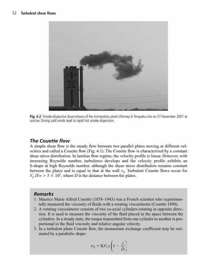
The Couette flowA simple shear flow is the steady flow between two parallel plates moving at different vel-ocities and called a Couette flow (Fig. 4.1). The Couette flow is characterized by a constantshear stress distribution. In laminar flow regime, the velocity profile is linear. However, withincreasing Reynolds number, turbulence develops and the velocity profile exhibits an S-shape at high Reynolds number, although the shear stress distribution remains constantbetween the plates and is equal to that at the wall �o. Turbulent Couette flows occur forVo D/� � 3 � 103, where D is the distance between the plates.

52 Turbulent shear flows

Remarks1. Maurice Marie Alfred Couette (1858–1943) was a French scientist who experimen-

tally measured the viscosity of fluids with a rotating viscosimeter (Couette 1890).2. A rotating viscosimeter consists of two co-axial cylinders rotating in opposite direc-

tion. It is used to measure the viscosity of the fluid placed in the space between thecylinders. In a steady state, the torque transmitted from one cylinder to another is pro-portional to the fluid viscosity and relative angular velocity.

3. In a turbulent plane Couette flow, the momentum exchange coefficient may be esti-mated by a parabolic shape:

�� � � K V yyD* 1

Fig. 4.2 Smoke dispersion downstream of the incineration plant chimney in Tempaku-cho on 27 November 2001 atsunrise. Strong cold winds lead to rapid hot smoke dispersion.

4.2 Jets and wakes

A jet flow is characterized by the developing flow and fully developed flow regions (Fig. 4.1).In the developing region, there is an undisturbed jet core with a velocity V � Vo, surroundedby developing shear layers in which momentum is transferred to the surrounding fluid. Thetransfer of momentum from the undisturbed jet core to the outer fluid is always associatedwith very-high levels of turbulence. The length of the developing flow region is about 6–12Dfor two-dimensional jets and 5–10D for circular jets discharging in a fluid at rest, where Dis the jet thickness or jet diameter (Fig. 4.1). Further downstream, the flow becomes fullydeveloped and the maximum velocity in a cross-section decreases with increasing distance.

In the developing flow of two-dimensional jets, the velocity in the undisturbed jet core isV � Vo, while the velocity profile in the developing shear layer is:

(4.1)

where y50 is the transverse location, V � Vo/2, Ks is a constant inversely proportional to therate of expansion of shear layer and erf is the error function.

In the fully developed region, the velocity distribution closely follows an analytical solu-tion of the momentum equation:

Two-dimensional jet, fully developed flow

(4.2a)

Circular jet, fully developed flow (4.2b)

where Vo is the initial jet velocity, D is the jet thickness and jet diameter for two-dimensional andcircular jets respectively. In equation (4.2b), y is the radial coordinate, sometimes denoted as r.

DiscussionThe developing shear layers are characterized by very-intense turbulence, well in excess oflevels observed in boundary layers and wakes. While the developing flow region is relativelyshort, the extent of the fully developed flow region, and the influence of the jet on the surroundings, may be felt far away.

A related flow situation is a wake behind an obstacle (Fig. 4.1). For example, the wake flowbehind a bridge pier (Fig. 4.3). Schlichting (1979) developed a complete analogy between jetand wake flows in the far field.

V

o

5.745

/1

1 0.125 18.5 V x D y

x

�

2

V

o

2 2.67

/1 tanh

V x D

yx

� � 7 7.

V

os

50 12

1 erf K

Vy y

x�

�

4.2 Jets and wakes 53

where K is the von Karman constant (K � 0.40), V* is the shear velocity, D is the dis-tance between plates and y is the distance normal to the plates (with y � 0 at oneplate). The result was found to be in good agreement with experiments (Schlichtingand Gersten 2000).

54 Turbulent shear flows

4.3 Boundary layer flows

A boundary layer is defined as the flow region next to a solid boundary where the flow field isaffected by the presence of the boundary. The concept was originally introduced by LudwigPrandtl (1904). In a boundary layer, momentum is gained from the main stream (or freestream) and contributes to the boundary layer growth. At the boundary, the velocity is zero.

A boundary layer is characterized by:

• its thickness defined in terms of 99% of the free-stream velocity:

where y is measured perpendicular to the boundary and Vo is the free-stream velocity.

( 0.99V o� �y V )

Discussion: momentum exchange coefficient in the developingflow region of a jetIn the developing flow region of a jet (e.g. Fig. 4.1 (top left) jet flow), the motion equa-tion can be analysed as a free-shear layer. For a plane shear layer, Goertler (1942) solvedthe equation of motion assuming a constant eddy viscosity �T across the shear layer:

where Ks is a constant which provides some information on the expansion rate of themomentum shear layer as the rate of expansion is proportional to 1/Ks. The analyticalsolution of the motion equation is equation (4.1) for two-dimensional jets.

For monophase free-shear layers, Ks equals between 9 and 13.5 with a generallyaccepted value of 11 (Rajaratnam 1976, Schlichting 1979, Schetz 1993). However,Brattberg and Chanson (1998) showed that the value of Ks is affected by the air bubbleentrainment rate in the developing region of plunging jet flows. They observed Ks to beabout 5.7 for plunging jet impact velocities ranging from 3 to 8 m/s.

�Ts2 o

1

4K� x V

Fig. 4.3 Wake behind bridge pier on the Mur river (Austria) in flood on 23 August 1999. Flow from right to left.

• the displacement thickness 1 defined as:

• the momentum thickness 2:

• the energy thickness 3:

3

2

1� �V V

o o0 d

V Vy

∫

20

1 dV V

o o

� �V V

y

∫

1 1 dV

o0� �

Vy

∫

4.3 Boundary layer flows 55

RemarkAlthough the boundary layer thickness is (arbitrarily) defined in terms of 99% of thefree-stream velocity, the real extent of the effects of boundary friction on the flow isprobably about 1.5–2 times .

Velocity distributionIn a turbulent boundary layer, the flow can be divided into three regions: an inner wall regionnext to the wall where the turbulent stress is negligible and the viscous stress is large, an outerregion where the turbulent stress is large and the viscous stress is small and an overlap regionsometimes called a turbulent zone.

For a turbulent boundary layer flow along a smooth boundary with zero pressure gradient,the velocity distribution follows:

Inner wall region: (4.3a)

Turbulent zone: (4.3b)

Outer region: (4.3c)

where V* is the shear velocity, � is the kinematic viscosity of the fluid, K is the von Karmanconstant (K � 0.40) and D1 is a constant (D1 � 5.5, Schlichting 1979). Equation (4.3b) iscalled the logarithmic profile or the ‘law of the wall’. Equation (4.3c) is called the ‘velocitydefect law’ or outer law.

y

0.1 to 0.15�V

VyVo

K

ln�

� �*

1

30 0 1to 70 and to 0.15*� �V y y

� .

V

*

*1

1K

ln V

V yD�

�

V y* 5�

�V

*

* V

V y�

�

56 Turbulent shear flows

Roughness effectsSurface roughness has an important effect on the flow in the wall-dominated region (i.e.inner wall region and turbulent zone). Numerous experiments showed that, for a turbu-lent boundary layer along a rough plate, the ‘law of the wall’ follows:

Turbulent zone: (4.5)

where D2 is a function of the type of the roughness height, roughness shape and spacing(e.g. Schlichting 1979, Schetz 1993). For smooth turbulent flows, D2 equals zero.

In the turbulent zone, the roughness effect (i.e. D2 � 0) implies a ‘downward shift’ ofthe velocity distribution (i.e. law of the wall). For large roughness, the so-called ‘lam-inar sublayer’ (i.e. inner region) disappears and the flow is said to be ‘fully rough’.

For fully rough turbulent flows in circular pipes with uniformly distributed sandroughness, D2, equals:

Fully rough turbulent flows in circular pipes

where ks is the equivalent sand roughness height.

Dk V

2 3 1K

ln s *� ��

y

0.1 to 0.15�V

*

*1 2

1K

ln V

V yD D�

�

ApplicationsIn a boundary layer flow, the velocity distribution may be approximated by a power law. Fora power-law velocity distribution:

(4.6)

the characteristic parameters of the boundary layers may be transformed. The displacementthickness and momentum thickness become:

(4.7)

1

11

� N

V

o

1/

V

yN

�

Coles (1956) showed that equation (4.3b) can be extended to the outer region by adding a‘wake law’ term to the right-hand side term:

Turbulent zone and outer region:

where � is the wake parameter and Wa is Coles’ wake function, originally estimated as(Coles 1956):

(4.4)Way y

�

2 sin 2�2

30 to 70 *�V y

�

V

*

*1

1K

ln K

V

V yD Wa

y�

�

�

(4.3d)

(4.8)

where N is the velocity exponent (equation (4.6)). And the shape factor becomes:

(4.9)

For two-dimensional turbulent boundary layers, Schlichting (1979) indicated that separation2

occurs for 1/ 2 � 1.8–2.4. Such a condition implies separation for N � 1.4–2.5.

Turbulent boundary layer development along a smooth flat plateFor turbulent flows in smooth circular pipes, the Blasius resistance formula (Blasius 1913)implies that the velocity profile follows exactly a 1/7th power-law distribution. Consideringa developing turbulent boundary layer on a smooth flat plate at zero incidence (and zero pres-sure gradient), the resistance formula deduced from the 1/7th power law of velocity distribu-tion implies (Schlichting 1979):

(4.10)

(4.11)

(4.12)

�2

1 5

xV x

0.036 o�

�

/

�1

1 5

xV x

0.046 o�

�

/

�xV x

0.37 o�

�

1 5/

1

2

2

�NN

2

1

(2 )�

NN N( )

4.3 Boundary layer flows 57

Discussion: momentum exchange coefficient in a turbulentboundary layerIn a smooth turbulent boundary layer, the mixing length l may be estimated as:

where tanh is the hyperbolic tangent function, K is the von Karman constant and is theboundary layer thickness (Schlichting and Gersten 2000, p. 557). The eddy viscosity �Tderives then from:

(3.3)�T2

V� l

y∂∂

l y

0.085 tanhK

0.085 �

2A deceleration of fluid particles leading to a reversed flow within a boundary layer is called a separation. Thedecelerated fluid particles are forced outwards and the boundary layer is separated from the wall.

4.4 Fully developed open channel flows

Fully developed open channel flows are commonly encountered in rivers and streams (Fig. 4.4).The flow motion is primarily controlled by the gravity force and boundary friction. At uni-form equilibrium, the gravity force component in the flow direction exactly equals the bound-ary friction force. The main differences between boundary layers and fully developed openchannel flows are: (1) the absence of momentum transfer at the open channel free surfacewhile momentum transfer does occur at the outer edge of a developing boundary layer(between the boundary layer itself and the free stream), and hence (2) the lack of boundary

58 Turbulent shear flows

Fig. 4.4 Mountain stream in Austria (22 August 1999). Looking upstream.

layer growth in fully developed open channel flows. Further air–water mass transfer mayoccur at the free surface, and high velocity open channel flows are characterized by signifi-cant free-surface aeration (‘white waters’) (Chapter 17).

The velocity distribution in fully developed turbulent open channel flows is given approxi-mately by Prandtl’s power law:

(4.13)

where y is the distance from the channel bed normal to the flow direction, d is the waterdepth, Vmax is the free-surface velocity and the exponent 1/N varies from 1/4 down to 1/12depending upon the boundary friction and cross-sectional shape. Chen (1990) developed acomplete analysis of the velocity distribution in open channel and pipe flow with reference toflow resistance. In uniform equilibrium flows, the velocity distribution exponent is related tothe flow resistance:

(4.14)

where f is the Darcy friction factor and K is the von Karman constant (K � 0.4). In engin-eering applications, a value N � 6 is reasonably representative of open channel flows forsmooth-concrete channels, although it must be remembered that N is a function of the flowresistance (e.g. equation (4.14)).

For a wide rectangular channel, the relationship between the mean flow velocity V and thefree-surface velocity Vmax derives from the continuity equation:

(4.15)

where q is the water discharge per unit width.

q Vd yN

NV d

d d

1V max� � �

0∫

Nf

K8

�

V

max

1/

V

yd

N

�

4.4 Fully developed open channel flows 59

Discussion: momentum exchange coefficient in fully developedopen channel flowsAssuming that the mixing length equals l � Ky, where K is the von Karman constant(K � 0.40) and assuming a linear variation of the turbulent shear stress across the flow,3

the eddy viscosity in a fully developed open channel flow becomes:

where V* is the shear velocity. Further discussion is developed in Chapter 16.

�T * K 1 � �V yyd

3That is, �(y) � �o(1 � y/d), where �o is the bed shear stress.

4.5 Mixing in turbulent shear flows

4.5.1 Presentation

In a shear flow, momentum is transferred from the region of high velocity to that of lowvelocity. The fluid tends to resist the shear associated with the transfer of momentum. Theshear stress is proportional to the rate of transfer of momentum. In turbulent flows, the appar-ent shear stress flow may be expressed as:

(3.2b)

where � is the fluid density and �T is the eddy viscosity or momentum exchange coefficient inturbulent flow. The momentum exchange coefficient �T is a function of the flow properties.

Equation (3.2b) implies that maximum shear occurs at the location of maximum velocitygradient in the direction normal to the flow. Note that this location corresponds to an inflec-tion point where: ∂2V/∂y2 � 0.

In turbulent mixing processes, mixing is related to the turbulent shear. The mixing coeffi-cients for momentum and mass are commonly assumed the same (see paragraph 7.1, Chapter7). For example, in open channel flows, the vertical mixing coefficient �V equals the momentumexchange coefficient �T. As a result, turbulent mixing is enhanced in regions of high momen-tum exchange coefficients. For example, near the singularity of a free-shear layer; at the nozzleedges of free jet; at half-depth in boundary layers and open channel flows. Practically, contam-inant injection should take place in such regions of large momentum exchange coefficient tomaximize the rate of turbulent mixing and dispersion.

4.5.2 Discussion: effects of contaminants on shear flows

The presence of contaminants does interact with turbulence (Figs 4.5 and 4.6). While turbu-lence enhances mixing and dispersion, contaminants in high proportion may inhibit, disturbor enhance turbulence characteristics: e.g. velocity distributions, turbulent velocity fluctu-ations, flow resistance.

Figure 4.5 illustrates some examples. In plunging jet flows, a large number of air bubblesmay be entrapped at the plunge point and diffuse downwards. The bubble diffusion layer andthe momentum shear layer do not coincide (Cummings and Chanson 1997, Brattberg andChanson 1998). The air–water shear flow properties differ from monophase flow data (Fig.4.5). The presence of air bubbles enhances the momentum spreading rate and the shear layeris located further outwards (i.e. away from the jet centreline).

The addition of dilute polymers and surfactants in water can be used to change the fluidproperties (viscosity, surface tension) and to modify the turbulence characteristics. Experi-mental studies showed that very-small concentration (few ppm) of dissolved polymer sub-stances can reduce the skin friction resistance in turbulent flows to as low as one-fourth ofthat in pure solvent. In pipelines and sewers, polymer additives are commonly used to reducethe skin drag, to enhance the discharge capacity: e.g. the Trans-Alaska oil pipeline, coal–waterpipe flows (Fig. 4.6b). Macromolecules of polymer and air bubbles interact with the turbu-lent structures, inducing a modification of the flow properties as compared to clear-waterflows (e.g. Gyr 1989, Bushnell and Hefner 1990, Chanson and Qiao 1994).

� �� TV

�∂∂y

60 Turbulent shear flows

In spillway flows, large amount of air bubbles are entrained and small air bubbles next tothe bottom modify the bottom shear stress, acting as macromolecules of polymer and indu-cing some drag reduction (Chanson 1994, Chapter 17). For example, at the downstream endof Karun dam spillway, flow velocities were observed to be in excess of 40 m/s that is nearly30% greater than predicted. The unexpected velocity increase was the result of some dragreduction caused by free-surface aeration.

4.5 Mixing in turbulent shear flows 61

Air bubble entrainmentat plunging jet

C, v

x

y

Inductiontrumpet

v

Developingshear layer

(air and water)

Air diffusion layer

Developing shear flow

Air entrainment

Entrainedair

Developing shear layer(monophase flow)

Ship motion

Ventilated cavity Gas film

Hullcross-section

KeelGas film Ventilation of ship hull

(gas-film lubrication)

y

C, v

v

C

Sedimentvolume fraction

profile

Sediment-laden flow

C,v

y

Airentrainment

in spillway flows

Fig. 4.5 Influence of entrained air bubbles on turbulent shear flows.

62 Turbulent shear flows

(a)

(b)

Fig. 4.6 Photographs of turbulent shear flows with high ‘contaminant’ fraction. (a) Sediment-laden flow down-stream of Mount St Helens (USA) with large (timber log) debris at a bridge crossing (courtesy of the US Army Corpsof Engineers, Portland District). (b) Trans-Alaska pipeline along the Richardson Highway just north of Paxson, AK inSeptember 2000 (courtesy of Steve STAPP). Completed in 1978, the pipeline (1.2 m diameter) is about 1300 km longand carries about 32 000 m3 of oil per day. Note the heat exchangers used to prevent thawing of the permafrost andthe zig-zag configuration to allow for expansion or contraction of the pipe because of temperature changes. Thedesign also allows for pipeline movement caused by a 8.5 earthquake. Drag reduction agent (DRA) is injected intothe oil to reduce the energy loss due to turbulence in the oil.

In laboratory and river flows, suspended sediment is observed sometimes to increase theflow velocity and to decrease the friction factor. Historical cases include observations of sus-pended silt flood flows in the Nile, Indus and Mississippi rivers. Chanson (1994, 1997)showed conclusively the cases of drag reduction with suspended-sediment flows.

Similar cases of drag reduction include ventilation downstream of hydrofoils for high-speed boats (40–80 knots) and gas-film lubrication of ship hull4 (Fig. 4.5).

4.6 Exercises

1. A circular jet (0.5 m diameter) discharges 0.6 m3/s of water in the middle of a lake.Assuming that the flow is driven by the initial jet momentum, calculate the flow velocity:(a) 15 m downstream on the jet centreline and (b) 20 m downstream and 8 m away from thecentreline (i.e. x � 20 m, r � 8 m).

2. During a storm, the wind blows over a sandy beach (0.5 mm sand particle). The windboundary layer is about 100 m high at the beach and the free-stream velocity at the outeredge of the wind boundary layer is 35 m/s. Calculate the shear velocity, the displacementand momentum thickness.

3. For the above problem (wind storm), calculate the virtual origin of the turbulent boundarylayer.

4.6 Exercises 63

(c)

Fig. 4.6 (Contd) (c) Air bubble entrainment at Shasta dam (USA) for low discharge on 6 August 1999 (courtesy ofDaniel Stephens).

4Controlled air injection along ship hull results in the reduction of skin friction drag.

4. The free-surface velocity in a river is 0.65 m/s and the water depth is 0.95 m. Assuming aDarcy friction factor f � 0.03, calculate the water discharge per unit width.

5. Considering a stream flow in a wide rectangular channel, the discharge per unit width is0.41 m2/s and the water depth is 1.9 m. Plot the velocity profile and momentum exchangecoefficient profile. Calculate the velocity and momentum exchange coefficient at 0.6 mabove the bed. Calculate the shear velocity as Chanson (1999a, pp. 74). Assume f � 0.041.

4.7 Exercise solutions

1. Vo � 3.056 m/s: (a) V � 0.58 m/s and (b) V � 0.056 m/s.2. First we must compute the bed shear stress or the shear velocity.

The Reynolds number Vo /� of the boundary layer is 2.3 � 108. The flow is turbulent. Asthe sand diameter is very small compared to the boundary layer thickness, the boundarylayer flow is assumed smooth turbulent. In a turbulent boundary layer along a smoothboundary, the mean bed shear stress equals:

where � is the fluid density, � is the kinematic viscosity, is the boundary layer thicknessand Vo is the free-stream velocity (at the outer edge of the boundary layer) (Schlichting1979, p. 637).

For the beach, it yields: �o � 0.27 Pa and V* � 0.47 m/s.Assuming a 1/7th power-law velocity distribution (i.e. smooth turbulent flow), the dis-

placement and momentum thicknesses equal: 1 � 12.5 m, 2 � 9.7 m.

� ��

o o

2

o

0.0225� VV

1 4/

64 Turbulent shear flows

NotesThe displacement thickness characterizes the displacement of the main flow due toslowing down of the fluid particles in the boundary layer. The momentum thicknesscharacterizes the displacement of free-stream momentum transport.

3. Virtual origin: �43 km upstream.4. q � 0.54 m2/s.5. Using equation (4.14), N � 5.6, Vmax � 0.2518 m/s, V (y � 0.6 m) � 0.205 m/s and

V* � 0.0154 m/s � �T(y � 0.6 m) � 0.0025 m2/s.

5

Diffusion: basic theory

SummaryIn this chapter the basic equation of molecular diffusion and simpleapplications are developed.

5.1 Basic equations

The basic diffusion of matter, also called molecular diffusion, is described by Fick’s law, firststated by Fick (1855). Fick’s law states that the transfer rate of mass across an interface nor-mal to the x-direction and in a quiescent fluid varies directly as the coefficient of moleculardiffusion Dm and the negative gradient of solute concentration. For a one-dimensionalprocess:

(5.1)

where.m is the solute mass flux and Cm is the mass concentration of matter in liquid. The

coefficient of proportionality Dm is called the molecular diffusion coefficient. Equation (5.1)implies a mass flux from a region of high mass concentration to one of smaller concentration.An example is the transfer of atmospheric gases at the free surface of a water body.Dissolution of oxygen from the atmosphere to the water yields some re-oxygenation.

The continuity equation (i.e. conservation of mass) for the contaminant states that spatialrate of change of mass flow rate per unit area equals minus the time rate of change of mass:

(5.2)

Replacing into equation (5.1), it yields:

(5.3a)∂∂

∂∂

Ct

DC

xm

mm

2 �

2

∂∂

∂∂

mx

Ct

0m �

m DCx

mm� �

∂∂

For diffusion in a three-dimensional system, the combination of equations (5.1) and (5.2)gives:

(5.3b)

Equations (5.3a) and (5.3b) are called the diffusion equations. It may be solved analyticallyfor a number of basic boundary conditions. Mathematical solutions of the diffusion equation(and heat equation) were addressed in two classical references (Crank 1956, Carslaw andJaeger 1959). Since equations (5.3a) and (5.3b) are linear, the theory of superposition may beused to build up solutions with more complex problems and boundary conditions: e.g.spreading of mass caused by two successive slugs.

∂∂

∂∂

∂∂

∂∂

Ct

DC

x

C

y

C

zm

mm

2m

2m

2 �

2 2 2

66 Diffusion: basic theory

Discussion: theory of superpositionIf the functions 1 and 2 are solutions of the diffusion equation subject to the respect-ive boundary conditions B1(1) and B2(2), any linear combination of these solutions,(a1 b2), satisfies the diffusion equation and the boundary conditions aB1(1) bB2(2). This is the principle of superposition for homogeneous differential equations.

Figure 5.1(a) and (b) illustrates a simple example. Figure 5.1(a) shows the solution ofdiffusion equation for the sudden injection of mass slug at the origin. By adding an uni-form velocity (current), the solution is simply the superposition of Fig. 5.1(a) plus theadvection of the centre of mass (Fig. 5.1(b)).

00

1

2

3

4

5

6

�1.5 �0.5 0.5 1.5

t � 0.01t � 0.1t � 0.3

M � 1, Dm � 0.2 Cm (x, t )

x(a)

Fig. 5.1 (a) Application of the theory of superposition. (a) Diffusion downstream a sudden mass slug injection. Gaussian distribution solutions of equation (5.4) for M � 1 and Dm � 0.2.

5.2 Applications

5.2.1 Initial mass slug

Initial mass slug introduced at t � 0 and x � 0A simple example is the one-dimensional spreading of a mass M of contaminant introducedsuddenly at t � 0 at the origin (x � 0) in an infinite (one-dimensional) medium with zerocontaminant concentration. The fluid is at rest everywhere (i.e. V � 0). The fundamentalsolution of the diffusion equation (5.3a) is:

for t � 0 (5.4)C x tM

D t

xD tm

m m

, ) exp4

( � �4

2

�

5.2 Applications 67

Notes1. Adolf Eugen Fick was a 19th Century German physiologist who applied Fourier’s

(1822) law of heat flow to molecular diffusion process.2. Typical values of molecular diffusion coefficients for solutes in water are in the range

5 �10�10 to 2 �10�9m2/s. Dm is a property of the fluid. For a given solvent (i.e.fluid), solute (i.e. tracer), concentration and temperature, Dm is a constant.

3. Turbulent enhances mixing drastically. Turbulent diffusion may be described also byequations (5.1)–(5.3) in which the molecular diffusion Dm is replaced by a turbulentdiffusion coefficient that is a function of the flow conditions (Chapter 7).

4. The theory of superposition may be applied to the diffusion equations (5.3a) and(5.3b) because it is linear.

00

1

2

3

4

5

6

�1.5 �0.5 0.5 1.5

t � 0.01t � 0.1t � 0.3

M � 1, Dm � 0.2, V � 1 Cm (x, t )

x(b)

Fig. 5.1 (b) Advection downstream a sudden mass slug injection for M � 1, Dm � 0.2, V � 1 – equation (6.5).

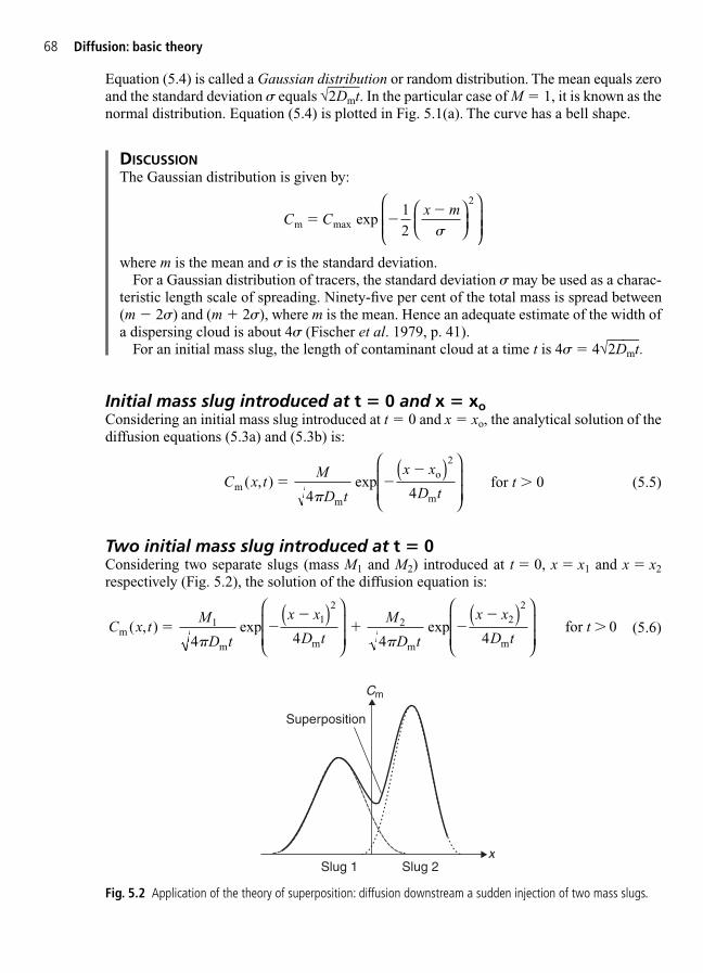
Equation (5.4) is called a Gaussian distribution or random distribution. The mean equals zeroand the standard deviation equals √

2Dmt. In the particular case of M � 1, it is known as the

normal distribution. Equation (5.4) is plotted in Fig. 5.1(a). The curve has a bell shape.

68 Diffusion: basic theory

DISCUSSIONThe Gaussian distribution is given by:

where m is the mean and is the standard deviation.For a Gaussian distribution of tracers, the standard deviation may be used as a charac-

teristic length scale of spreading. Ninety-five per cent of the total mass is spread between(m � 2) and (m 2), where m is the mean. Hence an adequate estimate of the width ofa dispersing cloud is about 4 (Fischer et al. 1979, p. 41).

For an initial mass slug, the length of contaminant cloud at a time t is 4 � 4√2Dmt.

C Cx m

m max exp

� ��1

2

2

Initial mass slug introduced at t � 0 and x � xoConsidering an initial mass slug introduced at t � 0 and x � xo, the analytical solution of thediffusion equations (5.3a) and (5.3b) is:

for t � 0 (5.5)

Two initial mass slug introduced at t � 0Considering two separate slugs (mass M1 and M2) introduced at t � 0, x � x1 and x � x2respectively (Fig. 5.2), the solution of the diffusion equation is:

(5.6)C x tM

D t

x x

D tM

D t

x x

D ttm

1

m

1

m

2

m

2

m

, ) 4

exp

4

exp

for 0( � ��

��

�� �

( )

( )

2 2

4 4

C x tM

D t

x x

D tmm

o

m

, ) 4

exp

( � ��

�

( )

2

4

Cm

Slug 2Slug 1

Superposition

x

Fig. 5.2 Application of the theory of superposition: diffusion downstream a sudden injection of two mass slugs.

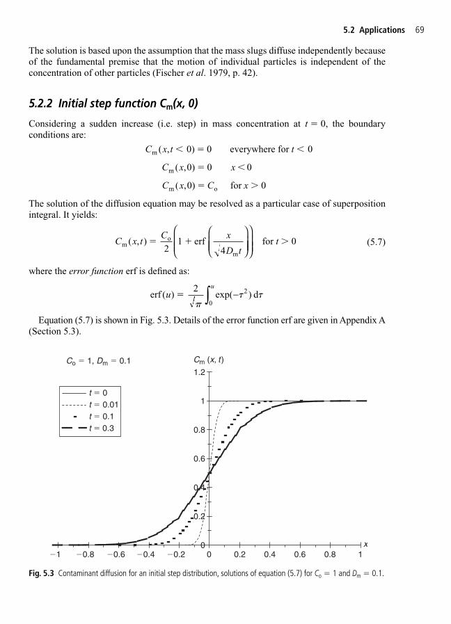
The solution is based upon the assumption that the mass slugs diffuse independently becauseof the fundamental premise that the motion of individual particles is independent of the concentration of other particles (Fischer et al. 1979, p. 42).

5.2.2 Initial step function Cm(x, 0)

Considering a sudden increase (i.e. step) in mass concentration at t � 0, the boundary conditions are:

The solution of the diffusion equation may be resolved as a particular case of superpositionintegral. It yields:

(5.7)

where the error function erf is defined as:

Equation (5.7) is shown in Fig. 5.3. Details of the error function erf are given in Appendix A(Section 5.3).

erf ( ) 2

exp( duu

��

� �−∫ 2

0)

C x tC x

D ttm

o

m

, ) 2

1 erf4

for 0( � �

C x C xm o( ,0) for 0� �

C x xm ( ,0) 0 0� �

C x t tm ( , 0) 0 everywhere for 0� � �

5.2 Applications 69

0

0.2

0.4

0.6

0.8

1

1.2

�1 �0.8 �0.6 �0.4 �0.2 0 0.2 0.4 0.6 0.8 1

t � 0t � 0.01t � 0.1t � 0.3

Co � 1, Dm � 0.1 Cm (x, t )

x

Fig. 5.3 Contaminant diffusion for an initial step distribution, solutions of equation (5.7) for Co � 1 and Dm � 0.1.

5.2.3 Sudden increase in mass concentration at the origin

The concentration is initially zero everywhere. At the initial time t � 0, the concentration issuddenly raised to Co at the origin x � 0 and held constant: Cm (0, t � 0) � Co. The analyt-ical solution of the diffusion equations (5.3a) and (5.3b) is:

(5.8)

Equation (5.8) is that of an advancing front (Fig. 5.4). At the limit t � �, Cm � Co everywhere.The result may be extended, using the theory of superposition, when the mass concentra-

tion at the origin Co varies with time. The solution of the diffusion equation is:

(5.9)C x tC x

D tx

t

mo

m

( , ) 1 erf4 (

d for 0� ��

��

∂∂

∞∫ ( )

)

�

� ��

C x t Cx

D txm o

m

, ) 1 erf for 0( � � �4

70 Diffusion: basic theory

NoteAt the origin, the mass concentration becomes a constant for t � 0: Cm(x � 0,t � 0) � Co/2.

0

0.2

0.4

0.6

0.8

1

1.2

0 0.2 0.4 0.6 0.8 1

t � 0.01t � 0.1t � 0.3

Co � 1, Dm � 0.15

Cm (x, t )

x

Fig. 5.4 Spread of a sudden concentration increase at the origin, solutions of equation (5.8) for Co � 1 andDm � 0.15.

DISCUSSIONThe step function (Section 5.2.2) is a limiting of the sudden increase in mass concentra-tion at the origin with constant mass concentration at the origin. In Section 5.2.2, themass concentration at the origin was Cm (x � 0, t � 0) � Co/2.

5.2.4 Effects of solid boundaries

When the spreading (e.g. of a mass slug) is restricted by a solid boundary, the principle ofsuperposition and the method of images may be used. The spreading pattern resulting from acombination of two mass slugs of equal strength includes a line of zero concentration gradi-ent midway between them (Fig. 5.5). Since the mass flux is zero according to Fick’s law(equation (5.1)), it can be considered as a boundary wall1 without affecting the other half ofthe diffusion pattern.

A simple example is the spreading of a mass slug introduced at x � 0 and t � 0, with awall at x � �L (Fig. 5.5). At the wall there is no transport through the boundary. That is, theconcentration gradient must be zero at the wall:

In order to ensure no mass transport at the wall, a mirror image of mass slug, with mass Minjected at x � �2L, is superposed to the real mass slug of mass M injected at x � 0. The flowdue to the mirror image of the mass slug is superposed onto that due to the mass slug itself.It yields:

(5.10)

Equation (5.10) is the solution of the superposition of two mass slugs of equal mass injectedat x � �2L and x � 0. It is also the solution of a mass slug injected at x � 0 with a solidboundary at x � �L.

C x tM

D t

xD t

x LD t

tmm

2

m

2

m

( , ) 4

exp exp( 2 )

for 0� � �

�� 4 4

m x L t DCx

x L( , ) 0 Boundary condition at the wall: mm� � � � � � �

∂∂

5.2 Applications 71

Cm

x

L L

Solidboundary

Realsource

Imagesource

Fig. 5.5 Spread of a sudden concentration increase at the origin with one boundary.

1There is no mass flux through a wall and any solid boundary.

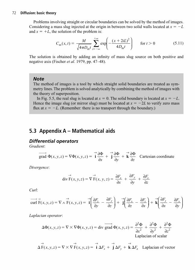
Problems involving straight or circular boundaries can be solved by the method of images.Considering a mass slug injected at the origin in between two solid walls located at x � �Land x � L, the solution of the problem is:

(5.11)

The solution is obtained by adding an infinity of mass slug source on both positive and negative axis (Fischer et al. 1979, pp. 47–48).

C x tM

D t

x iLD t

ti

mm

2

m

( , ) 4

2 )for 0� �

�

��

�exp

(4

∞

∞

∑

72 Diffusion: basic theory

NoteThe method of images is a tool by which straight solid boundaries are treated as sym-metry lines. The problem is solved analytically by combining the method of images withthe theory of superposition.

In Fig. 5.5, the real slug is located at x � 0. The solid boundary is located at x � �L.Hence the image slug (or mirror slug) must be located at x � �2L to verify zero massflux at x � �L. (Remember: there is no transport through the boundary.)

5.3 Appendix A – Mathematical aids

Differential operatorsGradient:

Divergence:

Curl:

Laplacian operator:

� � � � � � �F( , , ) F( , , ) Laplacian of vectorz

→ → → → →∇ ∇x y z x y z F F Fx yi j k

�� � � � � � ��

�

�

( , , ) ( , , ) div grad ( , , )

Laplacian of scalar

2 2 2x y z x y z x y z

x y z∇ ∇ ∂

∂∂∂

∂∂

2 2 2

curl F( , , ) F( , , ) x y z x y zFy

F

zFz

Fx

F

xFy

z y x z y x� � � � �∇ ∧ ∂∂

∂∂

∂∂

∂∂

∂∂

∂∂

→ → → →

i j k

div F( , , ) F( , , ) → →

∇ ∂∂

∂∂

∂∂

x y z x y zFx

F

yFz

x y z� �

grad ( , , ) , , Cartesian coordinate� � � ��

�

�

x y z x y zx y z

∇ ∂∂

∂∂

∂∂

→ → →( ) i j k

Error functionThe Gaussian error function, or function erf, is defined as:

Tabulated values are given in Table 5A.1. Basic properties of the function are:

where n! � 1 � 2 � 3 � … � n.The complementary Gaussian error function erfc is defined as:

erfc( ) 1 erf( ) 2

exp( ) du u t tu

� � � ��

2+∞

∫

erf( ) 1 exp( )

1 1

2

1 3

2

1 3 5

2

22 2

uu

u u x x� �

�� �

��

� �

� ( ) ( )

2 32

L

erf( ) 1

1!

2!

3!

3 5 7

u uu u u

� ��

�

��

� 3 5 7

L

erf( ) erf( )� � �u u

erf( ) 1� �

erf(0) 0�

erf( ) 2

exp( ) d2u t tu

� �� 0∫

5.3 Appendix A – Mathematical aids 73

NoteIn first approximation, the function erf(u) may be correlated by:

with a normalized correlation coefficient of 0.99952 and 0.9992 respectively. In manyapplications, the above correlations are not accurate enough, and Table 5A.1 should be used.

erf( ) tanh(1.198787 ) u u u� �� � � �

erf( ) (1.375511 0.61044 0.088439 0 22u u u u u� � � �)

Table 5A.1 Values of the error function erf

u erf(u) u erf(u)

0 0 1 0.84270.1 0.1129 1.2 0.91030.2 0.2227 1.4 0.95230.3 0.3286 1.6 0.97630.4 0.4284 1.8 0.98910.5 0.5205 2 0.99530.6 0.6309 2.5 0.99960.7 0.6778 3 0.999980.8 0.7421 � 10.9 0.7969

Notationx, y, z Cartesian coordinatesr, �, z polar coordinates∂/∂x partial differentiation with respect to the x-coordinate∂/∂y, ∂/∂z partial differential (Cartesian coordinate)∂/∂r, ∂/∂� partial differential (polar coordinate)∂/∂t partial differential with respect to time tD/Dt absolute derivativeN! N-factorial: N! � 1 � 2 � 3 � 4 � … � (N � 1) � N

Constantse constant such as Ln(e) � 1: e � 2.718 281 828 459 045 235 360 287� � � 3.141 592 653 589 793 238 462 643√

—2 √

—2 � 1.414 213 562 373 095 0488

√—3 √

—3 � 1.732 050 807 568 877 293 5

Mathematical bibliographyBeyer, W.H. (1982). CRC Standard Mathematical Tables. (CRC Press Inc.: Boca Raton, Florida, USA).Korn, G.A. and Korn, T.M. (1961). Mathematical Handbook for Scientist and Engineers. (McGraw-

Hill Book Comp.: New York, USA).Spiegel, M.R. (1968). Mathematical Handbook of Formulas and Tables. (McGraw-Hill Inc.:

New York, USA).

5.4 Exercises

1. A 3.1 kg mass of dye is injected in the centre of large pipe. In the absence of flow andassuming molecular diffusion only, calculate the time at which the mass concentrationequals 0.1 g/L at the injection point. Assume Dm � 0.89 � 10�2m2/s.

2. Considering a one-dimensional semi-infinite reservoir bounded at one end by a solid bound-ary (e.g. a narrow dam reservoir), a 5 kg mass slug of contaminant (Dm � 1.1 � 10�2m2/s)is injected 12 m from the straight boundary (e.g. concrete dam wall). Calculate the tracerconcentration at the boundary 5 min after injection. Estimate the maximum tracer con-centration at the boundary and the time (after injection) at which it occurs.

3. A 10 km long pipeline is full of fresh water. At one end of the pipeline, a contaminant isinjected in such a fashion that the contaminant concentration is kept constant and equals0.14 g/L. Assuming Dm � 1.4 � 10�3m2/s and an infinitely long pipe, calculate the time at which the pollutant concentration exceeds 0.007 and 0.01 g/L at 4.2 km from theinjection point.

5.5 Exercise solutions

1. t � 8500 s (2 h 21 min).2. (a) Cm � 2.8 � 10�5kg/m3 and (b) Cm � 0.2 kg/m3 and t � 6480 s (1.8 h).3. (a) t � 18 900 days (0.007 g/L) and (b) t � 22 000 days (0.01 g/L).

74 Diffusion: basic theory

6

Advective diffusion

SummaryThe basic equation of molecular advective diffusion is presented and simpleapplications are shown.

6.1 Basic equations

The previous section was developed assuming molecular diffusion with no transport and zerovelocity. That is, the fluid was assumed stationary, mass transport occurring by diffusiononly. Advection is the transport by an imposed current; a movement of a mass of fluid which enhances change in temperature or in other physical or chemical properties of fluid. In this section, we shall assume that transport by advection and diffusion are separate additive processes. That is, the diffusion takes place within the moving fluid as in a station-ary fluid.

The total mass transport rate equals:

(6.1)

where V is the fluid velocity. In equation (6.1), the first term (VCm) is the advective flux whilethe second term is the diffusive flux.

For a one-dimensional flow, the advective diffusion equation is:

(6.2a)

For a three-dimensional flow, it is:

(6.2b)∂∂

∂∂

∂∂

∂∂

∂∂

∂∂

∂∂

Ct

VCx

VCy

VCz

DC

x

C

y

C

zx y z

m m m mm

m m m � 2

2

2

2

2

2

∂∂

∂∂

∂∂

Ct

VCx

DC

xm m

m

2m

2 �

m VC DCx

m mm� �

∂∂

6.2 Basic applications

6.2.1 Advective diffusion of a sharp front

A simple one-dimensional application is a fluid moving in the x-direction at the velocity V,when the gradients in the y-direction are small (i.e. ∂/∂y �� ∂/∂x). The two-dimensionaladvective diffusion equation (6.2b) yields:

(6.3)

Considering a sharp front at t � 0, the boundary conditions are:

This is the case of a pipe filled with one fluid and being displaced by another fluid moving ata velocity V (Fig. 6.1). Practical applications include the cleaning of sewers with freshwaterand the steady injection of antibiotics in a blood vessel.

The solution of the advective diffusion equation is:

(6.4)

6.2.2 Initial mass slug introduced at t � 0 and x � 0

Another simple example is the sudden injection of a mass slug (mass M) at the origin att � 0. The solution of the problem is similar to the diffusion of an instantaneous mass sluginjection in a fluid at rest (i.e. equation (5.4)). When the velocity is non-zero, molecular diffusion takes place around the location of the centroid which is advected at a velocity V. At the time t, the location of centroid is X � Vt.

C x tC x Vt

D ttm

o

m

( , ) 1 erf

4for 0� �

��

2

C x xC x C x

m( , )0 0 00

for ( ,0) for m

� �� �

∂∂

∂∂

∂∂

Ct

VCx

DC

xm m

mm

2 �

2

76 Advective diffusion

DISCUSSIONThe advective diffusion theory is based upon the key assumption that diffusion andadvection are two separate additive processes (Fischer et al. 1979, p. 50). Hence the theory of superposition is applicable (Chapter 5).

RemarkPractical applications include an ‘idealized’ pipe filled with one fluid and being displacedby another, e.g. the cleaning of sewers with freshwater, the pumping of warm petroleumin an oil pipeline filled with cold fluid and the injection of antibiotics in blood vessels.

For a one-dimensional flow, the solution of the advective diffusion equation is:

(6.5)

Equation (6.5) is shown in Figure 5.1(b).

6.2.3 Transverse mixing of two streams with different concentrations

Considering the transverse mixing of two streams of different concentrations flowing side byside with the same velocity (Fig. 6.1), the diffusive transport in the x-direction is smaller thanthe advective transport. For the steady flow, the advective diffusion equation yields:

(6.6)

The boundary conditions are:

C y yC y C y

m

m o

for (0, ) for ( , )0 0 0

0� �� �

VCx

DC

y

∂∂

∂∂

mm

m2

�2

C x tM

D t

x VtD t

tmm

2

m

, ) exp )4

for ((

� ��

�4

0�

6.2 Basic applications 77

x

y

Cm

V

VCm � Co

Cm � Co

Cm � 0

Cm � 0

Growth of lateralmixing zone

xCm (x � 0, t � 0) � Co

Cm (x � 0, t � 0) � 0

Advective diffusionof a sharp front

Cm

xAdvective diffusion

downstream of massslug injection

Cm

Fig. 6.1 Basic applications of advective diffusion.

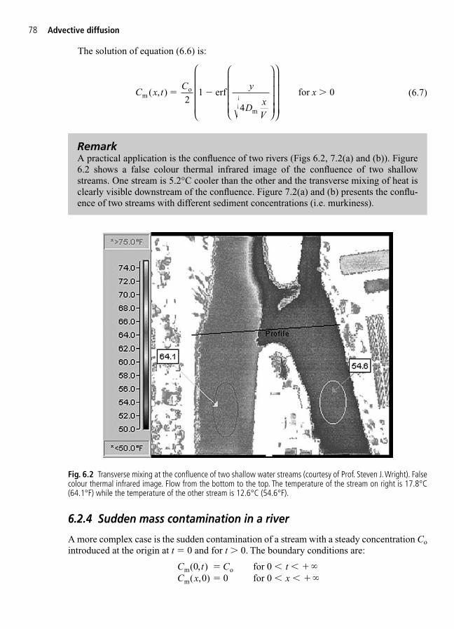
RemarkA practical application is the confluence of two rivers (Figs 6.2, 7.2(a) and (b)). Figure6.2 shows a false colour thermal infrared image of the confluence of two shallowstreams. One stream is 5.2°C cooler than the other and the transverse mixing of heat isclearly visible downstream of the confluence. Figure 7.2(a) and (b) presents the conflu-ence of two streams with different sediment concentrations (i.e. murkiness).

The solution of equation (6.6) is:

(6.7)C x tC y

DxV

xmo

m

( , ) 1 erf for � � �2

4

0

78 Advective diffusion

Fig. 6.2 Transverse mixing at the confluence of two shallow water streams (courtesy of Prof. Steven J. Wright). Falsecolour thermal infrared image. Flow from the bottom to the top. The temperature of the stream on right is 17.8°C(64.1°F) while the temperature of the other stream is 12.6°C (54.6°F).

6.2.4 Sudden mass contamination in a river

A more complex case is the sudden contamination of a stream with a steady concentration Cointroduced at the origin at t � 0 and for t � 0. The boundary conditions are:

C t C tC x x

m o

m

for 0 for 0

( , )( , )0

0 0� � � �� � � �

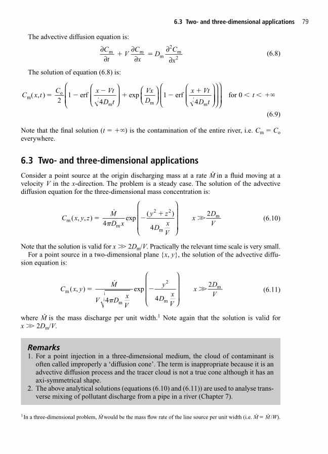
The advective diffusion equation is:

(6.8)

The solution of equation (6.8) is:

(6.9)

Note that the final solution (t � �) is the contamination of the entire river, i.e. Cm � Coeverywhere.

6.3 Two- and three-dimensional applications

Consider a point source at the origin discharging mass at a rate M� in a fluid moving at a velocity V in the x-direction. The problem is a steady case. The solution of the advective diffusion equation for the three-dimensional mass concentration is:

(6.10)

Note that the solution is valid for x �� 2Dm/V. Practically the relevant time scale is very small.For a point source in a two-dimensional plane {x, y}, the solution of the advective diffu-

sion equation is:

(6.11)

where M� is the mass discharge per unit width.1 Note again that the solution is valid forx �� 2Dm/V.

C x yM

V DxV

y

DxV

xDVm

m

2

m

m( , )

4

exp4

2

� � ��˙

�

C x y zMD x

y z

DxV

xDVm

m

2 2

m

m( , , ) 4

exp )

4 � �

��

˙ (�

2

C x tC x Vt

D t

VxD

x Vt

D ttm

o

m m m

( , ) 1 erf

4 exp 1 erf

4for 0 � �

� �

� � �

2

∂∂

∂∂

∂∂

Ct

VCx

DC

xm m

mm

2 �

2

6.3 Two- and three-dimensional applications 79

Remarks1. For a point injection in a three-dimensional medium, the cloud of contaminant is

often called improperly a ‘diffusion cone’. The term is inappropriate because it is anadvective diffusion process and the tracer cloud is not a true cone although it has anaxi-symmetrical shape.

2. The above analytical solutions (equations (6.10) and (6.11)) are used to analyse trans-verse mixing of pollutant discharge from a pipe in a river (Chapter 7).

1 In a three-dimensional problem, M� would be the mass flow rate of the line source per unit width (i.e. M� � M� /W).

6.4 Exercises

1. An initial mass slug (mass M � 1) is introduced suddenly at the origin at t � 0. AssumingDm � 0.2 and V � 1, (1) calculate the maximum mass concentration at t � 0.3 and (2) calculate the mass concentration for x � 0.07 and t � 0.3.

2. A pipeline is initially filled with clear water. At t � 0, contaminated waters (Co � 55 ppm,Dm � 2 � 10�9m2/s) are flushed into the pipeline at one end and the average flow velocity is 0.95 m/s. Estimate the width of the interface (defined between 5% and 95% ofthe initial concentration Co) 50 km downstream.

3. A one-dimensional stream (V � 0.35 m/s) is suddenly contaminated with a steady con-centration (Co � 185 ppm, Dm � 1.8 �10�1m2/s) introduced at t � 0. Estimate the timeat which the tracer concentration will be 20 ppm at 12 m from the injection.

Note: In the above exercises, large values of diffusion coefficients were used for simplicity ofcalculations and more meaningful results. Such values are not representative of solutes in water.

6.5 Exercise solutions

1. The solution of the problem is similar to the diffusion of an instantaneous mass slug injec-tion in a fluid at rest (i.e. equation (5.4)). When the velocity is non-zero, molecular diffu-sion takes place around the location of the centroid which is advected at a velocity V. At the time t, the location of centroid is X � Vt.

For a one-dimensional flow, the advective diffusion equation is:

(6.2a)

The solution is:

(6.5)

For t � 0.3, Cmax � 1.1 at x � 0.3. For t � 0.3 and x � 0.07, Cm � 0.15.

2. For a sharp front:

The distribution is symmetrical. For t � 50 000/0.95 s, x(Cm � 0.05Co) � 50 000 0.024 m and x(Cm � 0.95Co) � 50 000 � 0.024 m. Hence the interface width equals 4.8 cm.

3. t � 2 s.

C x tC x Vt

D tm

o

m

( , ) 1 erf

4� �

�

2

C x tM

D t

x VtD t

tmm

2

m

, ) exp )4

for ((

� ��

�4

0�

∂∂

∂∂

∂∂

Ct

VCx

DC

xm m

m

2m

2 �

80 Advective diffusion

7

Turbulent dispersion and mixing:1. Vertical and transverse mixing

SummaryIn this chapter, the basic equation of advective diffusion are applied to verticaland transverse mixing in natural river systems. Basic applications aredeveloped.

7.1 Introduction

Natural rivers are characterized by turbulent flows. Turbulence is generated by boundary frictionand it increases significantly the rate of mixing. While Chapters 5 and 6 consider moleculardiffusion and advection, the developments may be extended to turbulent dispersion and mixingwith few changes (Fischer et al. 1979, Lewis 1997). The molecular diffusion coefficient isreplaced basically by mixing coefficients: i.e. the vertical and transverse mixing coefficients�v and �t respectively. The turbulent advection and spread of particles in the longitudinaldirection is described by a dispersion coefficient K (Chapter 8).

When a tracer is injected into a homogeneous stream flow (Fig. 7.1), the advective transportmay be divided into three stages from upstream to downstream:

(a) mixing near the outlet driven by initial momentum and buoyancy,(b) transverse mixing of the effluent by turbulent transport,(c) longitudinal shear flow dispersion.

Longitudinaldispersion

Transverse mixing

Initial zone

Fig. 7.1 Mixing and dispersion of an effluent in a river.

(a)

(b)

Fig. 7.2 Examples of mixing in natural systems. (a) Confluence of Colorado River and Little Colorado River in the GrandCanyon of Arizona on 12 April 1966 (courtesy of Dr Lou Maher) – note the light (reddish) colour of the Little ColoradoRiver; the Colorado River has left its red mud behind the Glen Canyon Dam 60 miles upstream. (b) Confluence of theColorado and Dolorus Rivers, 20 miles North-East of Moab, Utah on 13 April 1966 (courtesy of Dr Lou Maher).(c) Pimpama Creek, Redlands, Queensland on 14 October 1999 (courtesy of the Waterways Scientific Services,Queensland Environment protection Agency) – looking upstream – note freshwater outfall near left bank during con-struction of a weir to reduce saltwater intrusion in the upper reach.

(c)

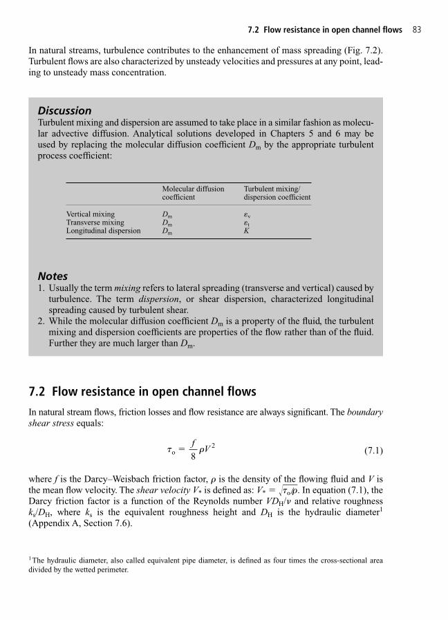
7.2 Flow resistance in open channel flows 83

DiscussionTurbulent mixing and dispersion are assumed to take place in a similar fashion as molecu-lar advective diffusion. Analytical solutions developed in Chapters 5 and 6 may be used by replacing the molecular diffusion coefficient Dm by the appropriate turbulent process coefficient:

Notes1. Usually the term mixing refers to lateral spreading (transverse and vertical) caused by

turbulence. The term dispersion, or shear dispersion, characterized longitudinalspreading caused by turbulent shear.

2. While the molecular diffusion coefficient Dm is a property of the fluid, the turbulentmixing and dispersion coefficients are properties of the flow rather than of the fluid.Further they are much larger than Dm.

Molecular diffusion Turbulent mixing/coefficient dispersion coefficient

Vertical mixing Dm �vTransverse mixing Dm �tLongitudinal dispersion Dm K

In natural streams, turbulence contributes to the enhancement of mass spreading (Fig. 7.2).Turbulent flows are also characterized by unsteady velocities and pressures at any point, lead-ing to unsteady mass concentration.

7.2 Flow resistance in open channel flows

In natural stream flows, friction losses and flow resistance are always significant. The boundaryshear stress equals:

(7.1)

where f is the Darcy–Weisbach friction factor, � is the density of the flowing fluid and V isthe mean flow velocity. The shear velocity V* is defined as: V* � �������. In equation (7.1), theDarcy friction factor is a function of the Reynolds number VDH/ and relative roughnessks/DH, where ks is the equivalent roughness height and DH is the hydraulic diameter1

(Appendix A, Section 7.6).

� �o2

8�

fV

1The hydraulic diameter, also called equivalent pipe diameter, is defined as four times the cross-sectional areadivided by the wetted perimeter.

For steady flows, the continuity equation states that: Q � VA where Q is the flow rate andA is the flow cross-sectional area. At uniform equilibrium (i.e. normal flow conditions), themomentum principle states that the boundary shear force equals exactly the weight forcecomponent in the flow direction. The uniform equilibrium flow velocity (i.e. normal velocity)equals:

(7.2)

and the average shear velocity becomes:

Uniform equilibrium flow (7.3)

where � is the bed slope.In natural systems, estimates of mixing and dispersion coefficients rely heavily upon accurate

estimate of the hydraulic properties of the river flow. Each student must know how to calculatebasic hydraulic properties before embarking into mixing and dispersion estimates.

V gD

*H sin�

4�

Vgf

D

8sinH�

4�

84 Turbulent dispersion and mixing: 1. Vertical and transverse mixing

Discussion: flow resistance estimate in natural streamsFlow resistance calculations in open channels must be performed in term of the Darcyfriction factor. In turbulent flows, however, the choice of the boundary equivalent rough-ness height is important. Hydraulic handbooks (e.g. Idelchik 1969, 1986) provide a selec-tion of appropriate roughness heights for standard materials. Main limitations of theDarcy equation for turbulent flows include:

• the friction factor may be estimated for relative roughness ks/DH � 0.05 and• classical correlations were validated for uniform-size roughness and regular roughness

patterns.

In simple words, the Darcy flow resistance equation is accurate in man-made channels withwell-defined roughness height. But flow resistance cannot be accurately predicted for com-plex roughness patterns: e.g. vegetation, composite cross-section, flood plain roughness(trees, houses, cars), shallow waters over large roughness, braided channels, meanderingchannel beds (Figs 3.1 and 7.2). See Chanson (1999a, pp. 85–91) for further discussion.

7.3 Vertical and transverse (lateral) mixing in turbulent river flows

In natural rivers, the flow is highly turbulent (Figs 3.1, 7.2 and 7.3). Fluid particles fluctuaterandomly while the stream is advected with a time-averaged velocity V. Figure 7.3 showsinstantaneous velocity measurements in a subtropical creek, in terms of the velocity modulusand direction. Note the data scatter. The random process may be modelled by a ‘random walk’model (Appendix B, Section 7.7).

Mixing is related to the turbulent shear: i.e. vertical mixing is induced by bottom frictionand transverse mixing is generated by bank roughness (Fig. 7.4). The mixing coefficients formomentum and mass are assumed the same.2 That is, the local mixing coefficient � equals themomentum exchange coefficient �T. This approximation is nearly always assumed in rivermixing and sediment suspension studies.

In fully developed open channel flows, the average vertical mixing coefficient (unit: m2/s)is about:

�v � 0.067 dV* (7.4)

The result is valid for a wide range of flows (e.g. Rutherford 1994, pp. 59–60).For fully developed open channel flows in straight rectangular channels, experimental obser-

vations (Fischer et al. 1979) suggest that the transverse mixing coefficient (unit: m2/s) is about:

�t � 0.15 dV* Straight rectangular channels (7.5)

A more recent review proposed: �t/dV* � 0.13 (Rutherford 1994, p. 102).In natural rivers, bends and sidewall irregularities enhance transverse mixing. Secondary

currents3 cause tracers to move in opposite directions at different depths and this behaviour

7.3 Vertical and transverse (lateral) mixing in turbulent river flows 85

0

5

10

15

20

25

30

35

40

45

1696 1697 1698 1699 1700 1701 1702 1703 1704 17050

0.02

0.04

0.06

0.08

0.1

0.12

0.14

0.16Velocity directionVelocity modulus

Time (s)

|V | (m/s)u (degree)

Fig. 7.3 Turbulent velocity fluctuations in a natural creek – instantaneous velocity modulus and direction in EprapahCreek, Queensland at 0.5 m beneath the free surface (after Chanson et al. 2003) – measurements conducted withan acoustic Doppler velocity meter recording 25 data per second.

2 This assumption is not strictly correct. Chanson (1997) discussed specifically the limitations of this assumptionfor air bubble entrainment in turbulent shear flows. See also Chapter 4, paragraph 4.5.2.3Secondary currents are perpendicular to the main current and they are caused by Reynolds stresses in any non-circular conduits. In natural rivers, they are significant at bends, and between a flood plain and the main channel.

greatly increases the rate of transverse mixing. For slowly meandering channels with moderatesidewall irregularities, a practical approximation is:

�t � 0.6 dV* Slowly meandering channels with moderate sidewall irregularities (7.6)

Larger transverse mixing coefficients are observed in sharply meandering rivers as shown in Figure 7.5 (see review in Fischer et al. 1979, pp. 109–112; Rutherford 1994, pp. 112–113).

86 Turbulent dispersion and mixing: 1. Vertical and transverse mixing

Vertical mixing

y

V

d

Transverse mixing

y

V

W

Fig. 7.4 Mixing in open channel flows.

Fig. 7.5 Stream meanders of the Elkhorn River on 16 April 1966 (courtesy of Dr Lou Maher).

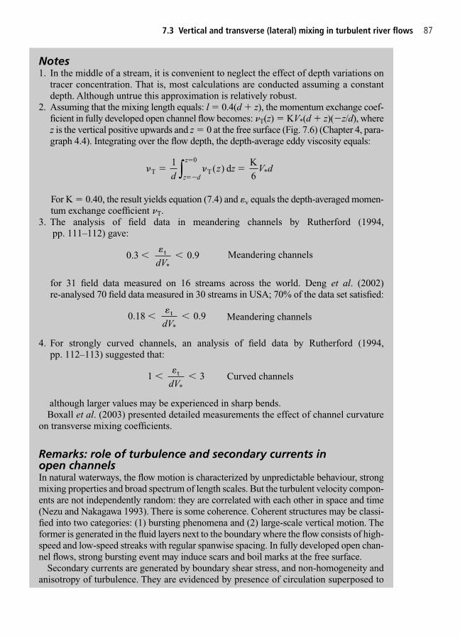
7.3 Vertical and transverse (lateral) mixing in turbulent river flows 87

Notes1. In the middle of a stream, it is convenient to neglect the effect of depth variations on

tracer concentration. That is, most calculations are conducted assuming a constantdepth. Although untrue this approximation is relatively robust.

2. Assuming that the mixing length equals: l � 0.4(d z), the momentum exchange coef-ficient in fully developed open channel flow becomes: �T(z) � KV*(d z)(�z/d), wherez is the vertical positive upwards and z � 0 at the free surface (Fig. 7.6) (Chapter 4, para-graph 4.4). Integrating over the flow depth, the depth-average eddy viscosity equals:

For K � 0.40, the result yields equation (7.4) and �v equals the depth-averaged momen-tum exchange coefficient �T.

3. The analysis of field data in meandering channels by Rutherford (1994,pp. 111–112) gave:

Meandering channels

for 31 field data measured on 16 streams across the world. Deng et al. (2002) re-analysed 70 field data measured in 30 streams in USA; 70% of the data set satisfied:

Meandering channels

4. For strongly curved channels, an analysis of field data by Rutherford (1994,pp. 112–113) suggested that:

Curved channels

although larger values may be experienced in sharp bends.Boxall et al. (2003) presented detailed measurements the effect of channel curvature

on transverse mixing coefficients.

Remarks: role of turbulence and secondary currents in open channelsIn natural waterways, the flow motion is characterized by unpredictable behaviour, strongmixing properties and broad spectrum of length scales. But the turbulent velocity compon-ents are not independently random: they are correlated with each other in space and time(Nezu and Nakagawa 1993). There is some coherence. Coherent structures may be classi-fied into two categories: (1) bursting phenomena and (2) large-scale vertical motion. Theformer is generated in the fluid layers next to the boundary where the flow consists of high-speed and low-speed streaks with regular spanwise spacing. In fully developed open chan-nel flows, strong bursting event may induce scars and boil marks at the free surface.

Secondary currents are generated by boundary shear stress, and non-homogeneity andanisotropy of turbulence. They are evidenced by presence of circulation superposed to

1 3t

*

��

�dV

0.18 0.9t

*

��

�dV

0 3. 0.9t

*

��

�dV

� ���

�

T T

0

* 1

( ) d K6d

z z V dz d

z

∫

DiscussionVertical mixing is the result of turbulence generated by bed friction. In natural streams,the time scale of vertical mixing (d2/�v) is nearly two orders of magnitude smaller thanthat of transverse mixing (W2/�t). Most rivers are much wider than deep (i.e. W/d � 10typically) while the vertical mixing coefficient is about 10 times smaller than the transversemixing coefficient. Often vertical and transverse mixing may be considered separately becausecontaminants are well mixed over the depth long before they are well mixed across thechannel.

Considering a natural stream with V � 1 m/s, d � 2 m, W � 30 m and V* � 0.05 m/s, thevertical mixing time scale (d2/�v) is about 600 s (10 min). The transverse mixing time scale(W 2/�t) is about 15 000 s (4.2 h).

Importantly: Diffusion coefficient estimates (equations (7.4)–(7.6)) were developed for grad-ually varied flows and uniform equilibrium flows. They do not apply to rapidly varied flow conditions. For example, hydraulic jumps are known for their very-strong mixing properties(Henderson 1966, Chanson 1999a). Experimental observations of vertical and transverse mix-ing coefficients in hydraulic jumps are presented and discussed in Appendix C (Section 7.8).

88 Turbulent dispersion and mixing: 1. Vertical and transverse mixing

the longitudinal fluid advection, and the flow streamlines often exhibit a spiral form. Instraight prismatic open channels, secondary currents are affected primarily by sidewalleffects, free-surface effects and bed roughness (Henderson 1996, p. 88; Nezu andNakagawa 1993, pp. 85, 91). The free-surface damps fluctuations normal to it. Secondarycurrents are responsible for large-size eddies which exhibit a coherent behaviour becausethey are generated by some interactions with the mean flow. They retain their structurewhile they are advected downstream over significant distances. In contrast small-scaleeddies are nearly isotropic and behave randomly.

In meandering channels, secondary currents are enhanced by the centrifugal force,and their velocity may be about 20–30% of mainstream velocity. A dominant feature isa helicoidal flow pattern which induces typically scour at the outer bend and depositionat the inner bank, yielding a quasi-triangular flow cross-section (Rozovskii 1957,Blanckaert and Graf 2001b).

RemarksTwo practical rules of thumb are:

• contaminants become well mixed vertically within a longitudinal distance of 50 timesthe water depth and

• tracers becomes well mixed across the channel about 100–300 channel widths down-stream of a point source near mid-stream (Rutherford 1994).

7.4 Turbulent mixing applications

Usually, vertical mixing is rapid in natural systems while transverse mixing is a much longerprocess because the channel width is much greater than the water depth. In many practical

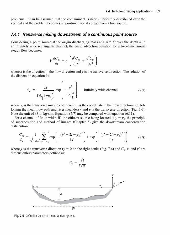
problems, it can be assumed that the contaminant is nearly uniformly distributed over the vertical and the problem becomes a two-dimensional spread from a line source.

7.4.1 Transverse mixing downstream of a continuous point source

Considering a point source at the origin discharging mass at a rate M.

over the depth d in an infinitely wide rectangular channel, the basic advection equation for a two-dimensionalsteady flow becomes:

where x is the direction in the flow direction and y is the transverse direction. The solution ofthe dispersion equation is:

(7.7)

where �t is the transverse mixing coefficient, x is the coordinate in the flow direction (i.e. fol-lowing the mean flow path and river meanders), and y is the transverse direction (Fig. 7.6).Note the unit of M

.in kg/s/m. Equation (7.7) may be compared with equation (6.11).

For a channel of finite width W, the effluent source being located at y � yo, the principle of superposition and method of images (Chapter 5) give the downstream concentrationdistribution:

(7.8)

where y is the transverse direction (y � 0 on the right bank) (Fig. 7.6) and Co, x� and y� aredimensionless parameters defined as:

CM

VdWo �˙

CC x

y i yx

y i yx

i

m

o

o2

o 1

4exp

2 )4

exp( 2

4�

��

� � �

� �

� �

�

� �

���

�

�

( )

∑

2

CM

VdxV

yxV

m

t

2

t

4

exp4

Infinitely wide channel�

�

�

�

˙

�

VCx

C

x

C

y

∂∂

∂∂

∂∂

mt

2m2

2m2

� �

7.4 Turbulent mixing applications 89

d

W

xy

z

Fig. 7.6 Definition sketch of a natural river system.

and the unit of M.

is kg/s.

7.4.2 Transverse mixing downstream of a mass slug injection

Considering a mass of contaminant M injected at t � 0 at the origin over the depth d in aninfinitely wide rectangular channel, the basic advection equation for a two-dimensionalunsteady flow is:

The solution of the advective diffusion equation is:

(7.9)

where y is the transverse direction (Fig. 7.6) and �t is the transverse mixing coefficient. Note that M is in kg, the mass injection is assumed to be instantaneous and the channel to beinfinitely wide.

7.4.3 Complete transverse mixing

Practically a reasonable distance for complete transverse mixing from a centreline discharge is:

(7.10)

where complete mixing is defined as the concentration is within 5% of its mean value every-where in the cross-section.

If the effluent is discharged at the side of the channel (e.g. Fig. 7.2(c)), the width overwhich the mixing take place is twice that for a centreline injection. Solid boundaries, such as

LV W

0.1 Complete mixing of centreline discharge2

t

��

C

Md

tx Vt y

tmt

2 2

t

exp( )

Infinitely wide channel��

��

�4 4�

∂∂

∂∂

∂∂

∂∂

Ct

VCx

C

x

C

ym m

t

2m2

2m2

� �

yy

W� �

xx

VW� �

� t

2

90 Turbulent dispersion and mixing: 1. Vertical and transverse mixing

Remarks1. Equation (7.9) assumes a velocity vector: Vx � V and Vy � 0. That is, x is the longi-

tudinal coordinate along the main flow direction.2. Turbulent diffusion takes place around the centroid which is advected at a velocity V.

At the time t, the location of centroid is x � Vt.

the channel bank, do lead to zero concentration gradients because there is zero mass flux. Areasonable distance for complete mixing from a side discharge is:

(7.11)

The latter may be rewritten as:

(7.11)

7.5 Discussion

7.5.1 Initial mixing

If the effluent discharge has enough momentum or buoyancy, the initial discharge forms aplume over some fraction of the cross-section. Further turbulent mixing occurs and it may becomputed by a superposition of line sources (see Chapter 5, equation (5.9)). It yields:

(7.12)

where Co(yo�) is the distributed source characterizing the initial mixing plume.

7.5.2 Applications

1. An industry releases 5 Mm3/day of effluents containing 250 ppm of a chemical near thecentre of a very wide, slowly meandering stream. The creek is 8 m deep, the mean velocity is0.5 m/s and the shear velocity is 0.1 m/s. Assuming that the effluent is completely mixed overthe vertical, determine the width of the plume and the maximum concentration 500 m down-stream of the discharge point.

CC y

x

y i yx

y i yx

yi

mo o o

2o

2

o0

1

4exp

( 2 )4

exp( 2 )

d��

��

� � � �

� �

� � �

��

���

�( )

�

∑∫ 4

xL

V W� �

� 0.4 Complete mixing of side discharget

2�

LV W

0.4 Complete mixing of side discharge2

t

��

7.5 Discussion 91

NotesRutherford (1994) proposed a slightly different definition for which ‘fully mixed’ isdefined as the ratio of minimum to maximum concentration across the channel is 98%.With this definition, it yields:

LV W

0.536 Side discharge2

t

��

LV W

0.134 Centreline discharge2

t

��

SolutionThe rate of input is:

M.

� 5 � 106m3/day � 250 ppm � 14.5 kg/s

The transverse mixing coefficient is about:

�t � 0.48 m2/s (equation (7.6))

The width of the plume may be approximated by

The maximum chemical concentration is: (or 47 ppm)(equation (7.7)). It occurs on the stream centreline.

2. A plant discharges a chemical at the side of a straight rectangular concrete channel. Thechannel is 50 m wide. The water flows at uniform equilibrium. The water depth equals 2.5 m,the velocity is 1.05 m/s and the bed slope is 0.0001. What is the channel length required forcomplete mixing? (Complete mixing is defined as to mean that the concentration of thechemical varies no more than 5% over the cross-section.)

SolutionThe shear velocity equals:

The transverse mixing coefficient is about:

�t � 0.0186 m2/s (equation (7.5))

As the effluent discharges at the side, the length for complete mixing equals:

L ~ 0.4V W2/�t � (0.4 � 1.05 � 502)/0.0186 � 5645 m

3. Considering two streams which flow together at a smooth junction, we will assume thatthe density is nearly the same and that mixing is caused by turbulence only. For example, twosources supply a treatment plant and the flow is blended before processing. Each sourcedelivers 15 m3/s. At the junction the water flows down a single rectangular channel (14 mwide) with a slope of 0.0008. The channel is concrete lined. Assuming a straight channel,what is the channel length required to provide complete mixing? Assume that uniform equi-librium flow conditions are achieved.

SolutionFirstly the hydraulic characteristics of the concrete channel must be calculated using themomentum principle. The process is iterative (Henderson 1966, Chanson 1999a). Assumingks � 1 mm (smooth concrete), it yields: V � 1.99 m/s, d � 1.07 m, V* � 0.09 m/s.

Secondly we assume that one stream is contaminated with a concentration Co and the otheris not (Cm � 0). After complete mixing, the concentration will be 0.5Co.

V gD* H sin 9.80 2.5 0.0001 0.0495 m/s� � � �/4 � �

C M Vd x Vm t3 / 4 / 0.047kg/m� � �˙ �

4 4 2 / 124mt � � �x V

92 Turbulent dispersion and mixing: 1. Vertical and transverse mixing

An upper limit of the length for complete mixing derives assuming that all the contamin-ation is discharged at the wall: L � 0.4VW2/�t. For a straight channel, it is about 108 000 m.The actual distance will be �10.8 km because the contaminants are discharged uniformlyover half of the channel width.

The exact solution may be achieved by applying a method of superposition based uponequation (5.7) or equation (7.12). (Fischer et al. (1979, pp. 118–119) developed the completeanalytical solution.) The final result is about 8.5 km for complete mixing (i.e. the concentra-tion is 5% of the mean everywhere).

7.6 Appendix A – Friction factor calculations

The laws of flow resistance in open channels are essentially the same as those in closed pipes(Henderson 1966, Chanson 1999a, 2004b). In laminar flows, the Darcy friction factor may beestimated as:

(7A.1)

where Re is the Reynolds number defined as: Re � �VDH/� and DH is the hydraulic diameter.4

In turbulent flows, the Darcy friction factor may be calculated from the Colebrook–Whiteformula:

(7A.2)

where ks is the equivalent sand roughness height. Note that the friction factor f appears onboth side of equation (7A.2) which must be solved by iterations. The friction factor may beinitialized by a less accurate expression called Altsul’s formula:

(7A.3)

7.7 Appendix B – Random walk model

In turbulent flows, the chaotic motion of the fluid and contaminant particles may be modelledby the ‘random walk’. The random walk model assumes that each particle is advected by themain current and displaced longitudinally, vertically and laterally by turbulent eddies. Withtime, the particles become separated further and further by the random (chaotic) motion.Each particle represents a mass unit and the number of particles in a given volume is a measure of concentration.

fkD Re

Re 0.1 1.46 100

s

H

� � �

1 441 10

/

1 2.0 log

2.51 10

s

Hf

kD Re f

Re� � � �3 71

1 104

.

fRe

Re 64

2 � � � 103

7.7 Appendix B – Random walk model 93

4The hydraulic diameter equals four times the flow cross-sectional area divided by the wetted perimeter. It is alsocalled the equivalent pipe diameter. Indeed, for a circular pipe flow, the hydraulic diameter equals exactly the pipediameter.

Random walk models simulate discrete mixing at a series of time steps �t. It is assumedthat turbulence is homogeneous and stationary: i.e. each step is uncorrelated to the previousone. For a long diffusion time T, the location of the centroid is X � VxT and the mean squaredisplacement 2

x of particles in the x-direction is:

2x � 2 DxT Long diffusion time (7B.1)

where Dx is the turbulent mixing coefficient in the x-direction. The probability that a particleis between x and (x �x) is given by:

(7B.2)

During a time step �t, a particle is advected in the x-direction by the ambient current Vx andmoved by the turbulent displacement. The net change in position �x equals:

(7B.3)

where RAND is a random number between �0.5 and 0.5. For long diffusion times and alarge number of particles, the random walk model yields a standard normal (Gaussian) dis-tribution. It may be extended to the y- and z-directions in a three-dimensional flow. Figure 7B.1presents a typical result for turbulent mixing of two particles, injected at the origin in a two-dimensional plane.

The random walk model can deal with boundaries, such as sea surface, bed and banks.When the random step taken by a particle reach a boundary, it may be allowed to reflect offthe boundary. Lewis (1997, pp. 149–150) illustrated the concept and presented one application.

� � � �x V t D tx x RAND 2

Probability( , ) 1

exp( )

Long diffusion time2

x Tx X

x x

� ��

2 2 2�

94 Turbulent dispersion and mixing: 1. Vertical and transverse mixing

�0.08

�0.06

�0.04

�0.02

0

0.02

0.04

0.06

10 20 30 40 50 60x

y

Particle 1

Particle 2

Current

Fig. 7B.1 Random walk of two particles suddenly injected at the origin in a two-dimensional plane for Vx � 1,Vy � 0, Dx � Dy � 1 and �t � 1.

7.8 Appendix C – Turbulent mixing in hydraulicjumps and bores

Most diffusion coefficient estimates (equations (7.4)–(7.6)) were developed for gra-dually varied flows and uniform equilibrium flows. They do not apply to rapidly varied flow

7.8 Appendix C – Turbulent mixing in hydraulic jumps and bores 95

Application to turbulent dispersionAccording to Langevin’s model of turbulent dispersion (Pope 2000, pp. 501–502), theLagrangian velocity auto-correlation function in turbulent flows5 is:

where TL is the Lagrangian time scale which is related to the dominant eddy size l and a typ-ical turbulent velocity u� by TL � l/u�, and t is the spacing between the two velocity points.

The variance of the momentum spread must then satisfy:

where t is the time, u�2 is the velocity variance for each particle. Initially, for t �� TL, thevelocity are highly correlated and the spread grows linearly with time: x � u�t. Forvery large times (TL �� t), it yields:

The latter is similar to equation (7B.1):

assuming that Dx � u�l.

Remarks1. Paul Langevin (1879–1946) was a French physicist, specialist in magnetism, ultra-

sonics and relativity. He was a member of the French pioneering team of atomicresearchers, which included Pierre and Marie Curie.

In 1905, Albert Einstein identified Brownian motion as due to imbalances in theforces on a particle resulting from molecular impacts from the liquid. Shortly there-after, Paul Langevin formulated a theory in which the minute fluctuations in the posi-tion of the particle were due explicitly to a random force. His approach had greatutility in describing molecular fluctuations in other systems, including non-equilibriumthermodynamics.

2. A Lagrangian method is the study of a process in a system of coordinates moving withan individual particle. For example, study of ocean currents with buoys. A differentmethod is the Eulerian method.

x xu T t u lt D t T t2 2 2 22L L� � � � � ��( )

x u T t 2 2L� �

x u T t Tt

T2 2 1 exp2

L LL

� � � � �

RTxx ( )

tt

L

exp� � �

5At a given time.

conditions: e.g. hydraulic jumps, positive surges, tidal bores. Experimental observations ofmixing coefficients in hydraulic jumps and bores are summarized in Table 7C.1.

In laboratory hydraulic jumps, the vertical diffusion coefficient of entrained air bubbleswas observed to be:

where d1 is the upstream water depth, V1 is the upstream flow velocity and Fr1 � V1/��gd1�(Chanson and Brattberg 2000). For dye and salt injection at the jump toe, complete verticaland transverse mixing was very rapid implying a transverse mixing coefficient estimate:6

In the Ord River, transverse sediment diffusivity �t was estimated to be about 0.71 m2/s(Table 7C.1). For comparison, measured transverse diffusivities were about 0.014–0.02 m2/sin the Severn River that has a similar water depth and possibly smaller width (Elliott et al.’swork, in Lewis 1997).

�� �t

1 1

0.14 5.9 V d

Fr� 1 7 7.

�� � ��v

1 1

2 4.5 10

V dFr� 5 0 8 51. .

96 Turbulent dispersion and mixing: 1. Vertical and transverse mixing

Table 7C.1 Experimental observations of lateral mixing in hydraulic jumps and bores

Experimental data Fr1 d1 Remarks(m/s) (m)

(1) (2) (3) (4)a (5)a

Chanson and 5.01 0.0158 1.5 � 10�2 – W � 0.25 m. Air bubble Brattberg (2000) 5.67 0.0158 6.2 � 10�2 – entrainment at jump toe

6.05 0.017 6.1 � 10�2 –6.32 0.014 5.0 � 10�2 –8.03 0.0158 5.2 � 10�2 –8.11 0.0158 3.0 � 10�2 –8.48 0.014 4.5 � 10�2 –

Bhargava and 7.30 0.0070 – 0.222 W � 0.3 m. Dye and Ojha (1990) 7.40 0.0072 – 0.227 salt injection at jump

6.37 0.0091 – 0.212 toe on centreline7.62 0.0109 – 0.1238.11 0.0119 – 0.1106.14 0.0150 – 0.1055.90 0.0167 – 0.1026.94 0.0162 – 0.0836.42 0.0180 – 0.081

Wolanski et al. (2001) 1.2 to 1.3 – – �t � 0.71 m2/sa Undular tidal bore of the Ord river (East branch)on 31 August 1999.W � 390 m (at meanstill water level)

Notes: aData re-analysis by the writer.

t�

V d1 1

v�

V d1 1

6Re-analysis of Bhargava and Ojha’s (1990) data.

7.9 Exercises

1. Considering a wide rectangular channel, the water depth is 3.2 m and the flow rate is2.8 m2/s. Assuming a gravel bed (ks � 12 mm), calculate the boundary shear stress and theshear velocity.

2. Water flows at uniform equilibrium in a 4.5 m wide, concrete-lined rectangular channel.The observed water depth is 0.85 m and the bed slope is 0.0011. Calculate the flow rate,the shear velocity and the vertical mixing coefficient.

3. A natural stream discharges 4.9 m3/s at equilibrium down a sandy bed slope (ks � 2 mm,slope: 0.0004). The channel width is 27 m. (a) Calculate the water depth and the shearvelocity. (b) Estimate the vertical and transverse mixing coefficient.

4. A sewage plant releases 250 m3/day of effluents containing 195 ppm of a chemical near theright bank of a wide, slowly meandering stream. The creek is 2.4 m deep and the bed slopeis 0.000 11. Calculate the flow rate and the shear velocity. Assuming that the effluent iscompletely mixed over the vertical, determine the width of the plume, the maximum con-centration 1200 m downstream of the discharge point and its location. Assume uniformequilibrium flow conditions in the river ( ks � 5 mm).

5. A barrel of arsenic (2.1 tonnes) falls accidentally from a trailer crossing a 1 km long wideriver. The river flows at 0.12 m/s and the water depth is 4.6 m (it is assumed that the containerfalls on the river centreline). Calculate the contaminant concentration 500 m downstreamof the injection point: (a) on the centreline, 1 h after the accident, (b) on the centreline, 1 h20 min after the accident and (c) 100 m from the centreline, 1 h 20 min after the accident.Assume V* � 0.0062 m/s. 1 tonne � 1 metric ton � 1000 kg.

6. Generate a random walk model using a spreadsheet (Appendix B). Assuming V � 1.2,Dx � 0.8 and �t � 1, study the dispersion of 100 particles in a one-dimensional flow. At atime T � 90, calculate the probability distribution function of the tracer concentration.(Perform the random walk computation using �t � 1. Plot the PDF using bins of �x � 0.2.)

7. A mass slug of chemical (15 kg) is released accidentally in a natural stream on the chan-nel centreline when a palette plunges into the creek at a crossing. The natural river has thefollowing channel characteristics during the event: water depth: 0.80 m, width: 72 m, bedslope: 0.0003, short grass: ks � 3 mm. Assume uniform equilibrium flow conditions in arectangular channel and assume a slowly meandering stream.

Calculate basic mixing and dispersion coefficients of the natural riverine system, andthe length of the initial zone.

7.10 Exercise solutions

1. V* � 0.043 m/s.2. Q � 6.14 m3/s, V* � 0.082 m/s, �v � 0.0046 m2/s.

7.10 Exercise solutions 97

Remarks1. A positive surge results from a sudden change in flow that increases the depth.2. When the surge is of tidal origin, it is usually termed a bore. The difference of name

does not mean a difference in principle (Henderson 1966, Chanson 1999a).

3. (a) d � 0.29 m, V* � 0.033 m/s.(b) �v � 6.4 �10�4m2/s, �t � 1.4 �10�3m2/s (straight channel) or �t � 5.7 �10�3m2/s

(slowly meandering channel).4. q � 2.6 m2/s, V � 1.09 m/s, V* � 0.050 m/s, �v � 8.05 �10�3m2/s, �t � 7.21 � 10�2m2/s

(slowly meandering channel).The half-plume width is calculated based upon the method of images, whereby the bank

is a line of symmetry. Using equation (7.7), the virtual mass discharge of sewer is: 2 �250 m3/day �195 ppm � 0.001 13 kg/s.

Maximum contaminant concentration occurs on the virtual centreline, that is on theright bank where the effluent is released: Cmax(x � 1200 m) � 1.37 �10�5kg/m3.

The width of the plume (i.e. measured from the right bank) is half of the width of thevirtual plume released on the centreline: i.e. 2 � 2��2�tx�/V� � 252 m.

5. Using equation (7.9):(a) Cm � 4.2 �10�9kg/m3 at x � 500 m, y � 0 and t � 1 h.(b) Cm � 1 �10�8kg/m3 at x � 500 m, y � 0 and t � 1 h 20 min.(c) Cm � 6.2 �10�22kg/m3 at x � 500 m, y � 100 m and t � 1 day.

6. Using a spreadsheet, set one row per particle. Apply equation (7B.3) to 100 discrete par-ticles. For T � 90, perform an histogram analysis. Note that the location of centroid isX � 90 � 1.2 � 108.

For a Gaussian probability distribution function, the square of the standard deviationequals:

(7B.1)

and the normal (Gaussian) probability distribution function satisfies:

(7B.2)

7. At uniform equilibrium flow: d � 0.792 m, V � 0.98 m/s, V* � 0.048 m/s.�v � 0.003 m2/s, �t � 0.023 m2/s (slowly meandering channel), K � 1405 m2/s (naturalriver).Length of initial zone: 22 km (centreline discharge).

Probability( , ) 1

2 144exp

( 108) 144

equation2

x T xx

� � � � �

�� 2

x xD T2 2 2 0.8 90 144 equation� � � � �

98 Turbulent dispersion and mixing: 1. Vertical and transverse mixing

8

Turbulent dispersion and mixing:2. Longitudinal dispersion

SummaryIn this chapter, Taylor’s dispersion theory is introduced. Then the dispersionequation is applied to natural river systems. Basic applications are discussed.

8.1 Introduction

Shear flow dispersion is the longitudinal stretching of matter caused by velocity shear. Forexample, in a circular pipe, the velocity is larger on the centreline than near the wall. As aresult, the longitudinal spread of matter is faster on the centreline, leading to greater separ-ation of the effluent particles than by molecular diffusion. The rate of separation is caused bythe difference in advective velocity. Turbulent shear dispersion is also called longitudinal dis-persion. The basic theory of shear dispersion is derived from Taylor’s (1953, 1954) work.

Considering a tracer released from an instantaneous line source, the contaminant travelsmore slowly near the channel banks than in the centreline (Fig. 8.1). As a result, the initialline source is stretched longitudinally and spreading occurs both along and across the chan-nel as illustrated in Fig. 8.1. The rate of longitudinal dispersion reflects the balance betweenvelocity shear which acts to spread tracer along the channel and transverse mixing which promotes uniform concentrations across the channel and hence counteracts the effects ofvelocity shear (Rutherford 1994, pp. 178–179).

DiscussionTaylor’s theory is based upon the assumptions that turbulent mixing processes occur ina similar fashion as molecular diffusion, and it is valid only away from the injectionpoint: i.e. downstream of the initial zone (see paragraph 8.2 and Fig. 7.1). Further mostsolutions of the dispersion equation imply that there are constant mixing conditions,uniform velocity distribution and idealized reflection at the channel boundaries. Thismonograph is no exception.

8.2 One-dimensional turbulent dispersion

For one-dimensional flows, the dispersion equation is:

(8.1)

where Cm and V are the mean concentration and velocity respectively, and K is the dispersioncoefficient (unit: m2/s). Equation (8.1) implies that turbulent mixing and longitudinal disper-sion take place in a similar fashion as molecular advective diffusion. Further most solutionsassume constant mixing conditions (K constant), uniform velocity distribution (V constant)

∂∂

∂∂

∂∂

Ct

VCx

KC

xm m

2m

2 �

100 Turbulent dispersion and mixing: 2. Longitudinal dispersion

y

Velocityprofile

V

Line sourceinjection

Spreadingby

turbulentdiffusion

Cross-sectionalaveraged

concentration x

t � 0 t � t1

Fig. 8.1 Sketch of longitudinal dispersion of a line source injection by vertical and transverse velocity shear in a river.

Longitudinal dispersion and transverse mixing are strongly interrelated. Longitudinaldispersion is a delicate balance between velocity shear spreading tracer longitudinallyversus transverse mixing promoting uniform transverse concentration. It will be shownthat the longitudinal dispersion coefficient K is inversely proportional to the transversemixing coefficient �t: i.e. K � 1/�t.

NoteSir Geoffrey Ingram Taylor (1886–1975) was a British fluid dynamicist professor basedin Cambridge. He established the basic developments of shear dispersion (Taylor 1953,1954).

and idealized reflection of mass at channel boundaries.1 Note that equation (8.1) is valid onlyaway from the injection point.2 That is, downstream of the initial zone.

The dispersion coefficient K is a function of the flow conditions (e.g. velocity profile). Forturbulent flows in circular pipes, K equals:

K � 5.05 DV* Turbulent pipe flow (8.2)

where V* is the shear velocity and D is the pipe diameter.For turbulent open channel flows, the dispersion coefficient is:

K � 5.93 dV* Turbulent open channel flow (8.3)

where d is the flow depth. The result is based upon the logarithmic velocity distribution(Chapter 4, paragraph 4.3).

Equation (8.2) was first developed by Taylor (1954) while equation (8.3) was developed byElder (1959). In any case the dispersion coefficient is proportional to a characteristic lengthscale times the shear velocity, V*, which is a measure of shear stress and velocity gradientnear the boundary (Chapter 7, paragraph 7.2). In the next section, however, it is shown thatequations (8.2) and (8.3) are not appropriate for natural river systems.

8.3 Longitudinal dispersion in natural streams

8.3.1 Basic equation

After a contaminant is well mixed across the entire cross-section, the final stage of the mix-ing process is the reduction of longitudinal gradients by dispersion. However, if the effluentdischarge is a constant, there is no need to be concerned by dispersion. Longitudinal disper-sion is important in applications characterized by non-constant effluent releases: e.g. acci-dental spill a quantity of pollutant, daily variations of sewage effluents released by a watertreatment plant.

The advection–dispersion equation for one-dimensional flow is:

(8.1)

Considering the instantaneous slug release (mass M, side discharge) in a one-dimensionalflow, the solution of the dispersion equation (8.1) is a Gaussian distribution:

x� � 0.4 (8.4)

where A is the channel cross-section, t is the time of travel (or elapsed time since tracerrelease) and V is the flow velocity.

CM

A Kt

x VtKtm

2

( )

� ��

4 4�exp

∂∂

∂∂

∂∂

Ct

VCx

KC

xm m

2m

2 �

8.3 Longitudinal dispersion in natural streams 101

1See Chapter 9 for further discussion on dead zones.2For t �� 0.4 , where D is the characteristic length scale (e.g. pipe diameter) and K is the dispersion coefficient.D

K

2

DiscussionWhen applying Taylor’s dispersion analysis to natural rivers, one must understand that theadvective dispersion equation (8.1) is a one-dimensional analysis and it does not apply to theinitial zone (Fig. 8.1). The initial zone is characterized by vertical and transverse mixing.Basically the dispersion equation (8.1) does not apply for x� � x�t/(VW 2) � 0.4 with a sidedischarge (Chapter 7, paragraph 7.4.3).

For 0.4 � x� � 1, the dispersion equation is valid and the longitudinal concentration dis-tribution is skewed, decaying towards a Gaussian distribution. For x� � 1, the solution of thedispersion equation is a Gaussian distribution (equation (8.4)). In both the cases, the virtualorigin of the chemical cloud is approximately (Fischer et al. p. 136, Fig. 5.14):

Virtual origin (8.5)

In the case of a slug of contaminants (mass M) released suddenly at the origin into a nat-ural stream, the longitudinal length of the cloud after the initial mixing may be estimated asfour times the standard deviation � ��2Kt�. That is:

x� � 0.4(3) (8.6)

The peak concentration within the dispersed cloud equals:

x� � 0.4 (8.7)

8.3.2 Dispersion coefficient in natural rivers

In natural rivers, the coefficient of dispersion was found to be about: K/(dV*) � 9–7500(Fischer et al. 1979, pp. 125–127). Such values are well in excess of Elder’s (1959) estimate(equation (8.3)). Natural rivers are characterized by transverse variations of the velocitywhich enhance dispersion. Figure 8.2 shows a typical cross-sectional velocity distribution ina stream.

CM

A KxV

max

4

�

�

Length of cloud 4 4 2 ( / )2

t� �� �

Kx V W

V0 07.

xx

V W� �

�� 0.07t

2

102 Turbulent dispersion and mixing: 2. Longitudinal dispersion

3For a side discharge.

Comments1. Many natural streams have bends, sandbars, sidepools and other natural changes, and

every irregularity in the channel contributes to longitudinal dispersion. Some chan-nels may be so irregular that no reasonable approximation of dispersion is possible:e.g. a mountain stream consisting of pools and riffles (see Chapter 9, paragraph 9.2).

2. Sometimes the virtual origin of the tracer cloud may be neglected for calculationsperformed far downstream (x� �� 0.07). This is often the case, like in the ‘frozencloud’ approximation method (paragraph 8.4).

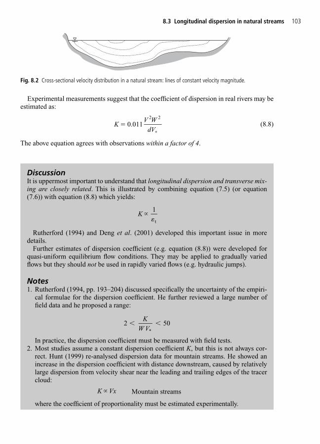
Experimental measurements suggest that the coefficient of dispersion in real rivers may beestimated as:

(8.8)

The above equation agrees with observations within a factor of 4.

KV W

dV 0.011

2 2

�∗

8.3 Longitudinal dispersion in natural streams 103

Fig. 8.2 Cross-sectional velocity distribution in a natural stream: lines of constant velocity magnitude.

DiscussionIt is uppermost important to understand that longitudinal dispersion and transverse mix-ing are closely related. This is illustrated by combining equation (7.5) (or equation(7.6)) with equation (8.8) which yields:

Rutherford (1994) and Deng et al. (2001) developed this important issue in moredetails.

Further estimates of dispersion coefficient (e.g. equation (8.8)) were developed forquasi-uniform equilibrium flow conditions. They may be applied to gradually variedflows but they should not be used in rapidly varied flows (e.g. hydraulic jumps).

Notes1. Rutherford (1994, pp. 193–204) discussed specifically the uncertainty of the empiri-

cal formulae for the dispersion coefficient. He further reviewed a large number offield data and he proposed a range:

In practice, the dispersion coefficient must be measured with field tests.2. Most studies assume a constant dispersion coefficient K, but this is not always cor-

rect. Hunt (1999) re-analysed dispersion data for mountain streams. He showed anincrease in the dispersion coefficient with distance downstream, caused by relativelylarge dispersion from velocity shear near the leading and trailing edges of the tracercloud:

Mountain streams

where the coefficient of proportionality must be estimated experimentally.

K Vx �

2 50� �K

W V*

K 1

t

��

ApplicationsApplication No. 1Considering the dispersion of a slug of chemical injected at the side of a stream, the riverflows at uniform equilibrium. The channel is 50 m wide, it may be assumed rectangular andthe river bed is made of small gravels (ks � 5 mm). The water depth is 2.4 m and the bedslope is 0.0003.

(a) Estimate the longitudinal dispersion coefficient.(b) Calculate the channel length required to provide complete transverse mixing. (Note that

Taylor’s dispersion analysis does not apply in the initial zone characterized by transversemixing.)

(c) Estimate the peak concentration that will be observed 38 000 m downstream of the injec-tion point, and the length of the chemical cloud at the time when the peak passes thatpoint. (Assume a contaminant mass of 10 kg.)

SolutionFirstly the hydraulic characteristics of the river flow must be calculated using the momentumprinciple. The process is iterative (Henderson 1966, Chanson 1999a). For ks � 5 mm, ityields: V � 1.73 m/s, Q � 207 m3/s and V* � 0.080 m/s.

(a) The longitudinal dispersion coefficient equals:

(equation (8.8))

(b) A reasonable distance for complete mixing from a side discharge is: L � 0.4V W 2/�t, orx� � 0.4. In the absence of further information, the transverse mixing coefficient is esti-mated as for a slowly meandering stream with some wall roughness: �t � 0.6dV* � 0.6 �2.4 � 0.080 � 0.1152 m2/s (equation (7.6)). It yields:

L � 0.4 � 1.73 � 502/0.1152 � 15 000 m

(c) At the observation station where x � 38 000 m, x� � x�t(VW 2) � 38 000 � 0.1152/(1.73 � 502) � 1.01. We may assume the longitudinal concentration distribution to beGaussian. The length of the real cloud may be estimated by assuming that the cloudstarted with zero variance at x� � 0.07 (i.e. x � 2600 m).

K 0.011 1.73

429 m /s

22� �

�

��

502 4 0 080

2

. .

104 Turbulent dispersion and mixing: 2. Longitudinal dispersion

3. Deng et al. (2001) re-analysed a number of field observations for straight, naturalrivers. They proposed an estimate for the longitudinal dispersion coefficient:

Straight rivers

where Et is basically a dimensionless transverse mixing coefficient:

EVV

Wdt 0.145

13520

� *

.

1 38

KE

W V

d V

0.158 t

5/3 2

2/3�

*

The variance of the cloud at the observation station is basically a linear function of time forx� � 0.4. It yields: 2 � 2Kt � 2K (38 000 � 2600)/1.73 � 17.6 � 106m2.

For a Gaussian distribution, the length of the cloud may be approximately estimated as 4:

Length of cloud: 4 � 16 800 m Equation (8.6)

The peak concentration is:

Equation (8.7)

Application No. 2Rhodamine WT dye is released as a slug into the Bremer River to estimate the longitudinaldispersion coefficient. The dye cloud is monitored at four locations. At the first two, the cloudwas poorly mixed and not amenable to a simple analysis. At the third location (located3800 m downstream of the release point), a dye concentration Cm � 0.0004 kg/m3 was meas-ured 45 min after the initial release. The peak dye concentration Cmax � 0.0025 kg/m3 passedthe fourth measuring station, located 2300 m downstream of the release point, 39 min afterthe initial release.

Calculate the longitudinal dispersion coefficient.

SolutionCalculations are conducted between the third and fourth measurement locations, assumingthat the dye is well mixed and that there is no decay of rhodamine (source/sink). All the cal-culations derive from:

(8.4)

At the fourth measuring station, maximum concentration is obtained for (x � Vt) � 0.That is, the average velocity of the flow is: V � 2300/(39 � 60) � 0.98 m/s.

At the third measuring station, equation (8.4) yields:

At the fourth measuring station, equation (8.4) yields:

It yields: K � 70 m2/s.Note that the peak concentration for t � 45 min satisfies:

M

A K4 2700 0.0025

3945

0.00233kg/m3

� �� �

0 00254

. 2340

��

M

A K�

0 00044 4

. exp 2700

(3800 0.98 2700) 2700

2

��

�� �

�

M

A K K�

CM

A Kt

x VtKtm

4

� �

�

�exp

( )2

4

CM

A KxV

m6 3

4

2.4

7.7 10 kg/m� �

� � � � �

� � �

�

10

50 4 3 14 429380001 73

..

8.3 Longitudinal dispersion in natural streams 105

8.4 Approximate models for longitudinal dispersion

8.4.1 The ‘frozen cloud’ approximation

In many applications, advection dominates dispersion (i.e. x �� K/V) and maximum tracerconcentration occurs at t � x/V. The concept of frozen cloud assumes that no longitudinaldispersion occurs during the time taken for the tracer to pass a sample site. Although notstrictly correct in natural streams, the frozen cloud approximation is commonly made whenanalysing longitudinal dispersion data.

With that approximation, hypothetical concentration versus time prediction at a fixed pointx may be estimated as:

x� � 1 (8.9)

where x is fixed (constant) and Cmax is estimated from equation (8.7). Equation (8.9) isderived from equation (8.4) for the frozen cloud approximation.

The prediction of concentration versus distance at a given time t may be estimated as:

(8.10)

where t is fixed (constant). Note that equation (8.10) derives from equation (8.4).

C xM

A K txV

x Vt

K txV

m

2

( )

4 2

( )

2

�

�

��

��

exp

4

C t Cx Vt

KxV

m max

2

( ) ( )

� ��

exp4

106 Turbulent dispersion and mixing: 2. Longitudinal dispersion

DISCUSSIONLet us consider a tracer cloud such that the centroid passes a location x � x1 at t � T1. Thefrozen cloud assumption implies: x1 � VT1. Equation (8.4) expresses the relationship:Cm � Cm(x, t). Under the frozen cloud approximation, it may be transformed to yield:

Concentration versus time at a fixed location x1 (equation (8.9))

Concentration versus distance at a fixed time T1 (equation (8.10))

Rutherford (1994, pp. 209–215) discussed the limitations of the frozen cloud assumption.In any case, equations (8.9) and (8.10) may apply only downstream of the initial region(x� �� 0.07), assuming constant dispersion coefficient K and uniform velocity V.

C x C x Tx x

VM

A K TxV

x x

K TxV

m m 1 11

1

12

1

( ) ;

4 2

( )

2

� �

�

�

��

�

�

exp

4

C t C x V T t TM

A KT

x VtKTm m 1 1 1

1

12

1

( ) ( ); 4

( )� � � �

�( ) exp

� 4

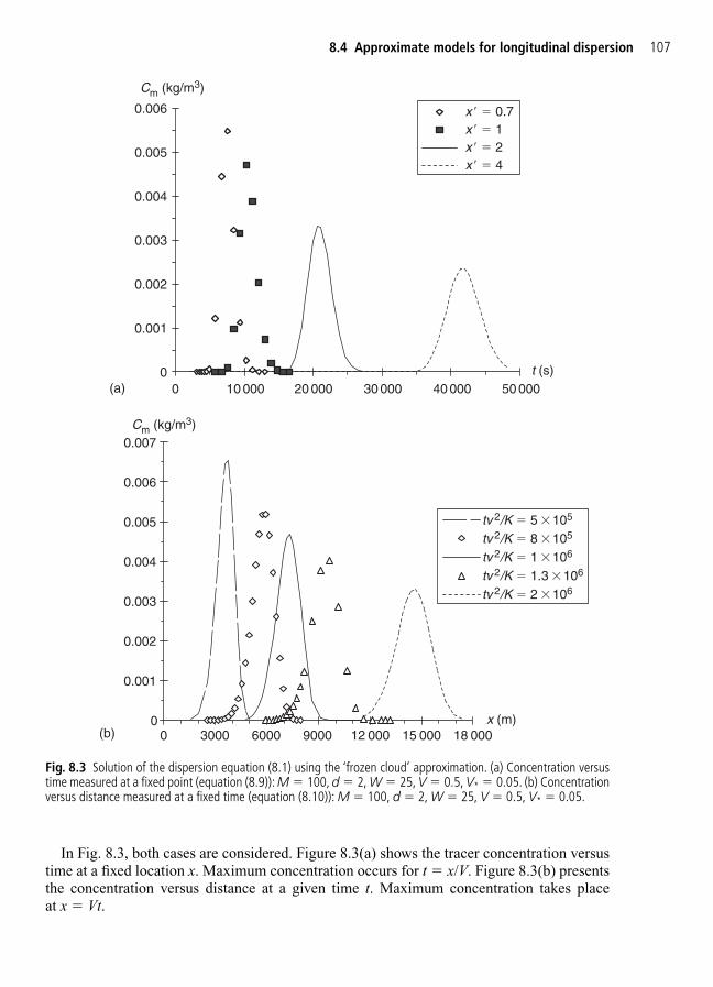
In Fig. 8.3, both cases are considered. Figure 8.3(a) shows the tracer concentration versustime at a fixed location x. Maximum concentration occurs for t � x/V. Figure 8.3(b) presentsthe concentration versus distance at a given time t. Maximum concentration takes place at x � Vt.

8.4 Approximate models for longitudinal dispersion 107

0

0.001

0.002

0.003

0.004

0.005

0.006

0 10 000 20 000 30 000 40 000 50 000

x � � 0.7x � � 1x � � 2x � � 4

Cm (kg/m3)

t (s)(a)

0

0.001

0.002

0.003

0.004

0.005

0.006

0.007

0 3000 6000 9000 12 000 15 000 18 000

Cm (kg/m3)

x (m)

tv 2/K � 5 �105

tv 2/K � 8 �105

tv 2/K � 1 �106

tv 2/K � 1.3 �106

tv 2/K � 2 �106

(b)

Fig. 8.3 Solution of the dispersion equation (8.1) using the ‘frozen cloud’ approximation. (a) Concentration versustime measured at a fixed point (equation (8.9)): M � 100, d � 2, W � 25, V � 0.5, V* � 0.05. (b) Concentrationversus distance measured at a fixed time (equation (8.10)): M � 100, d � 2, W � 25, V � 0.5, V* � 0.05.

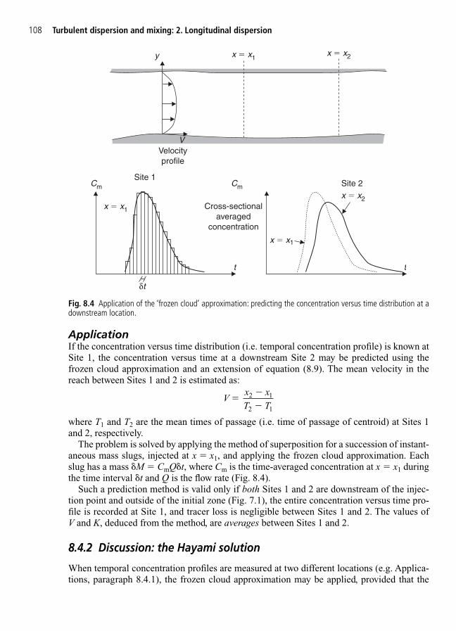
108 Turbulent dispersion and mixing: 2. Longitudinal dispersion

V

y

Velocityprofile

x � x1 Cross-sectionalaveraged

concentration

t

Cm Cm

δt

Site 1

t

Site 2

x � x1

x � x2

x � x2x � x1

Fig. 8.4 Application of the ‘frozen cloud’ approximation: predicting the concentration versus time distribution at adownstream location.

ApplicationIf the concentration versus time distribution (i.e. temporal concentration profile) is known atSite 1, the concentration versus time at a downstream Site 2 may be predicted using thefrozen cloud approximation and an extension of equation (8.9). The mean velocity in thereach between Sites 1 and 2 is estimated as:

where T1 and T2 are the mean times of passage (i.e. time of passage of centroid) at Sites 1 and 2, respectively.

The problem is solved by applying the method of superposition for a succession of instant-aneous mass slugs, injected at x � x1, and applying the frozen cloud approximation. Eachslug has a mass �M � CmQ�t, where Cm is the time-averaged concentration at x � x1 duringthe time interval �t and Q is the flow rate (Fig. 8.4).

Such a prediction method is valid only if both Sites 1 and 2 are downstream of the injec-tion point and outside of the initial zone (Fig. 7.1), the entire concentration versus time pro-file is recorded at Site 1, and tracer loss is negligible between Sites 1 and 2. The values of V and K, deduced from the method, are averages between Sites 1 and 2.

8.4.2 Discussion: the Hayami solution

When temporal concentration profiles are measured at two different locations (e.g. Applica-tions, paragraph 8.4.1), the frozen cloud approximation may be applied, provided that the

Vx xT T

2 1

2 1

��

�

measurement sites are outside of the initial zone, that the entire concentration versus timedistributions are recorded and that the tracer loss is negligible between the two sites. Themeasurement outcomes are reach-averaged values of V and K.

The dispersion equation (8.1) has another solution in addition to equation (8.4). It is calledthe Hayami solution (Barnett 1983):

x� � 0.4 (8.11)

Equation (8.11) can be used to predict the downstream propagation of a tracer cloud withoutneeding to invoke the frozen cloud approximation.

8.5 Design applications

8.5.1 Application No. 1

Investigations are undertaken for a scheme to abstract drinking water from the Logan River tosupply Cedar Grove. One important design consideration is the time that it would take for a pol-lutant accidentally discharged into the river (e.g. following a rail/road tanker accident) to reachthe intake site and the length of the time that concentrations would be above some critical value.To assist the design of off-river storage, calculations are based upon the following assumptions.

Q � 250 m3/s Average width: 45 m Average bed slope: 0.0009 Gravel bed: ks � 25 mm

Consider the case of road bridge 35 km upstream of the abstraction site and the instantaneousinjection of 250 kg of a chemical which is likely to cause water treatment problems at con-centrations exceeding 5 mg/m3.

SolutionHydraulic calculations at uniform equilibrium flow conditions yield:

d � 2.15 m V* � 0.132 m/s

The mean travel time is:

tmean � 13565 s (3.8 h) (equation (8.4))

Transverse mixing coefficient:

�t � 0.17 m2/s (equation (8.6))

Longitudinal dispersion coefficient:

K � 523 m2/s (equation (8.8))

Dimensionless distance:

x� � 1.14

CMx

AVt Kt

x VtKtm

2

4

( )� �

�

�exp

4

8.5 Design applications 109

DISCUSSIONEquation (8.11) is simply equation (8.4) multiplied by x/(Vt). It satisfies the boundarycondition that Cm(x � 0, t � 0) � 0, for all values but t � 0 when an instantaneous slugof mass M is introduced at the origin. Rutherford (1994, pp. 214–215) presented a com-parison between the Taylor and Hayami solutions (i.e. equations (8.4) and (8.11)).

Length of complete mixing:

L � 12.3 km assuming side discharge (Section 7.4.2)

Peak concentration at proposed intake:

Cmax � 2.74 �10�4kg/m3 (274 mg/m3) (equation (8.7))

The peak concentration is above the acceptable limit by a factor of 55.Applying equation (8.9), the concentration at the intake reaches 5 mg/m3 about 2.8 h after

injection. It will drop below this limit about 5.1 h after injection (Fig. 8.5).

8.5.2 Application No. 2

Norman Creek, in Southern Brisbane, has the following channel characteristics during aflood event:

Water depth: 1.16 m Width: 55 m Bed slope: 0.002 Short grass: ks � 3 mm

A mass slug of chemical (7.5 kg) is released accidentally in the natural stream on the chan-nel centreline (when a truck plunge into the creek at a crossing):

(a) Calculate the hydraulic characteristics of the stream in flood.(b) Predict the dispersion coefficient and the length of the initial zone.

A measurement station is located 25 km downstream of the injection point.

110 Turbulent dispersion and mixing: 2. Longitudinal dispersion

0

50

100

150

200

250

1.5 2 2.5 3 3.5 4 4.5 5 5.5

Cm (mg/m3)

t (h)

Equation (8.4)

Fig. 8.5 Cross-sectional averaged chemical concentrations predicted at the proposed intake (x � 35 km).

Note that, although the true longitudinal concentration distribution is skewed for x� � 1,the shape of the cloud is approaching the Gaussian distribution for x� � 0.7. For x� � 1,the frozen cloud approximation may be used (Fig. 8.3).

(c) Calculate the maximum tracer concentration at that station and the arrival time.(d) The detection limit of the chemical is 0.2 mg/m3. Calculate the length of time during which

the chemical will be detectable at the measurement station.

Assume uniform equilibrium flow conditions in a rectangular channel. Neglect vertical mixing and assume a slowly meandering stream.

SolutionUniform equilibrium flow calculations yield:

V � 3.13 m/s V* � 0.148 m/s

The dispersion coefficient equals:

K � 1890 m2/s (equation (8.8))

The length of the initial zone equals: 9170 m (Chapter 7, paragraph 7.4.3).

The maximum tracer concentration at the measurement station equals: 8.5 � 10�6kg/m3

(equation (8.7)) and it is observed 8000 s (2 h 13 min) after injection.The length of the time during which the chemical is detectable of the measurement station

equals: 7810 s. That is, between 53 min and 3 h after injection (using a frozen cloud approximation).

8.6 Exercises

1. A natural stream has the following channel characteristics: flow rate: 18.5 m3/s, waterdepth: 0.786 m, width: 15 m, bed slope: 0.001, gravel: ks � 5 mm. Assume uniform equi-librium flow conditions in a rectangular channel. Neglect vertical mixing and assume aslowly meandering stream.

A barrel of dye (2.2 kg) is suddenly released in the natural stream from the channelbank (i.e. side). A measurement station is located 18 km downstream of the injection point.(a) Calculate the maximum mass concentration in the cross-section located at 500 mdownstream of the injection point. (b) Calculate the maximum tracer concentration at that station and the arrival time. (c) The detection limit of the chemical is 0.3 mg/m3.

8.6 Exercises 111

DISCUSSIONNote the near-critical flow conditions (Fr � 0.9) which are likely to be characterized byfree-surface undulations. The undular flow pattern may induce scour beneath wavetroughs (Kennedy 1963, Chanson 2000), while secondary currents may enhance mixingand dispersion.

Note that the measurement station is located outside of the initial zone. Hence the dispersion theory is valid.

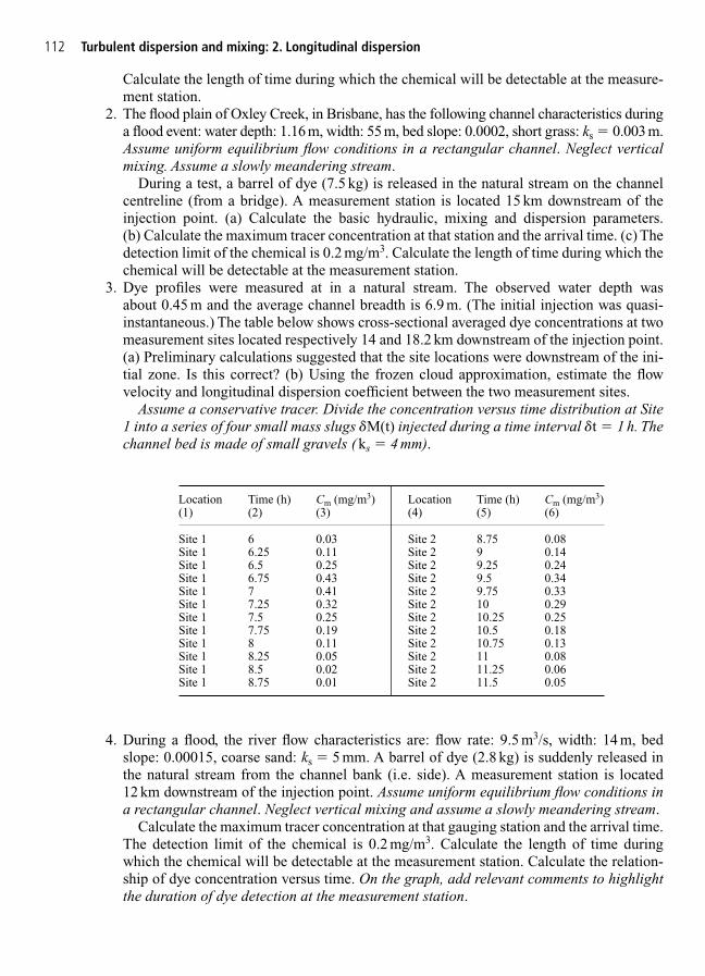
Calculate the length of time during which the chemical will be detectable at the measure-ment station.

2. The flood plain of Oxley Creek, in Brisbane, has the following channel characteristics duringa flood event: water depth: 1.16 m, width: 55 m, bed slope: 0.0002, short grass: ks � 0.003 m.Assume uniform equilibrium flow conditions in a rectangular channel. Neglect verticalmixing. Assume a slowly meandering stream.

During a test, a barrel of dye (7.5 kg) is released in the natural stream on the channelcentreline (from a bridge). A measurement station is located 15 km downstream of theinjection point. (a) Calculate the basic hydraulic, mixing and dispersion parameters. (b) Calculate the maximum tracer concentration at that station and the arrival time. (c) Thedetection limit of the chemical is 0.2 mg/m3. Calculate the length of time during which thechemical will be detectable at the measurement station.

3. Dye profiles were measured at in a natural stream. The observed water depth was about 0.45 m and the average channel breadth is 6.9 m. (The initial injection was quasi-instantaneous.) The table below shows cross-sectional averaged dye concentrations at twomeasurement sites located respectively 14 and 18.2 km downstream of the injection point.(a) Preliminary calculations suggested that the site locations were downstream of the ini-tial zone. Is this correct? (b) Using the frozen cloud approximation, estimate the flowvelocity and longitudinal dispersion coefficient between the two measurement sites.

Assume a conservative tracer. Divide the concentration versus time distribution at Site1 into a series of four small mass slugs M(t) injected during a time interval t � 1 h. Thechannel bed is made of small gravels ( ks � 4 mm).

112 Turbulent dispersion and mixing: 2. Longitudinal dispersion

Location Time (h) Cm (mg/m3) Location Time (h) Cm (mg/m3)(1) (2) (3) (4) (5) (6)

Site 1 6 0.03 Site 2 8.75 0.08Site 1 6.25 0.11 Site 2 9 0.14Site 1 6.5 0.25 Site 2 9.25 0.24Site 1 6.75 0.43 Site 2 9.5 0.34Site 1 7 0.41 Site 2 9.75 0.33Site 1 7.25 0.32 Site 2 10 0.29Site 1 7.5 0.25 Site 2 10.25 0.25Site 1 7.75 0.19 Site 2 10.5 0.18Site 1 8 0.11 Site 2 10.75 0.13Site 1 8.25 0.05 Site 2 11 0.08Site 1 8.5 0.02 Site 2 11.25 0.06Site 1 8.75 0.01 Site 2 11.5 0.05

4. During a flood, the river flow characteristics are: flow rate: 9.5 m3/s, width: 14 m, bedslope: 0.00015, coarse sand: ks � 5 mm. A barrel of dye (2.8 kg) is suddenly released inthe natural stream from the channel bank (i.e. side). A measurement station is located12 km downstream of the injection point. Assume uniform equilibrium flow conditions ina rectangular channel. Neglect vertical mixing and assume a slowly meandering stream.

Calculate the maximum tracer concentration at that gauging station and the arrival time.The detection limit of the chemical is 0.2 mg/m3. Calculate the length of time duringwhich the chemical will be detectable at the measurement station. Calculate the relation-ship of dye concentration versus time. On the graph, add relevant comments to highlightthe duration of dye detection at the measurement station.

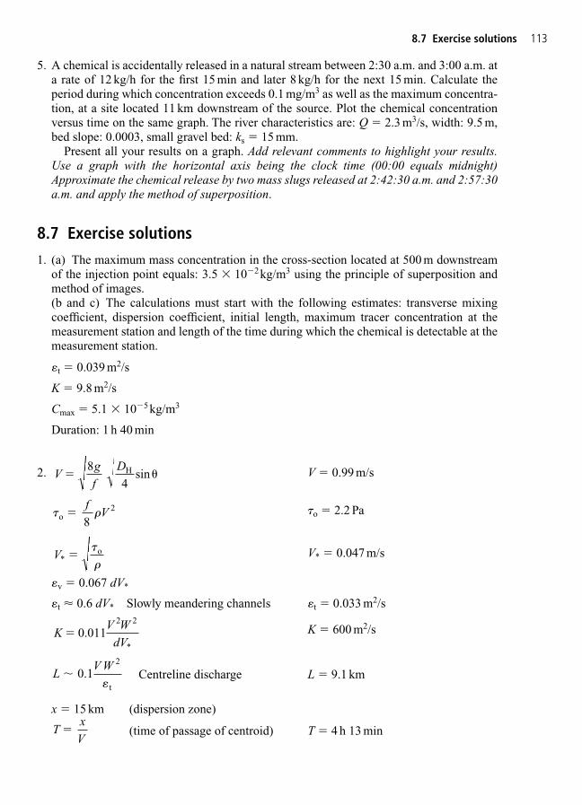
5. A chemical is accidentally released in a natural stream between 2:30 a.m. and 3:00 a.m. ata rate of 12 kg/h for the first 15 min and later 8 kg/h for the next 15 min. Calculate theperiod during which concentration exceeds 0.1 mg/m3 as well as the maximum concentra-tion, at a site located 11 km downstream of the source. Plot the chemical concentrationversus time on the same graph. The river characteristics are: Q � 2.3 m3/s, width: 9.5 m,bed slope: 0.0003, small gravel bed: ks � 15 mm.

Present all your results on a graph. Add relevant comments to highlight your results.Use a graph with the horizontal axis being the clock time (00:00 equals midnight)Approximate the chemical release by two mass slugs released at 2:42:30 a.m. and 2:57:30a.m. and apply the method of superposition.

8.7 Exercise solutions

1. (a) The maximum mass concentration in the cross-section located at 500 m downstreamof the injection point equals: 3.5 � 10�2kg/m3 using the principle of superposition andmethod of images.(b and c) The calculations must start with the following estimates: transverse mixingcoefficient, dispersion coefficient, initial length, maximum tracer concentration at themeasurement station and length of the time during which the chemical is detectable at themeasurement station.

�t � 0.039 m2/s

K � 9.8 m2/s

Cmax � 5.1 � 10�5kg/m3

Duration: 1 h 40 min

2. V � 0.99 m/s

�o � 2.2 Pa

V* � 0.047 m/s

�v � 0.067 dV*

�t � 0.6 dV* Slowly meandering channels �t � 0.033 m2/s

K � 600 m2/s

Centreline discharge L � 9.1 km

x � 15 km (dispersion zone)

(time of passage of centroid) T � 4 h 13 minTxV

�

LV W

0.12

t

��

KV W

dV 0.011

2 2

�*

V* o��

�

� �o2 �

fV

8

Vgf

D

4H� �

8sin

8.7 Exercise solutions 113

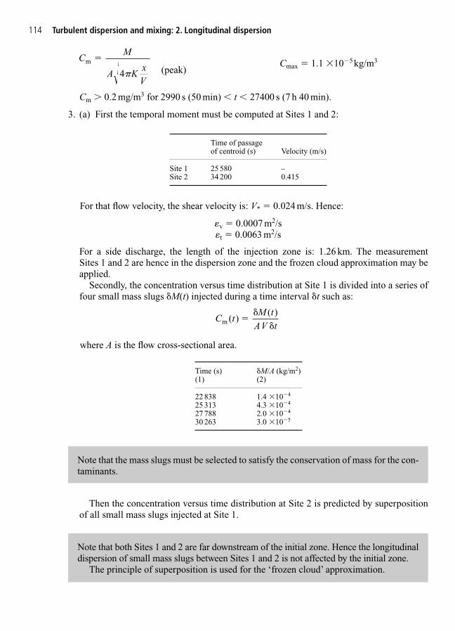
For that flow velocity, the shear velocity is: V* � 0.024 m/s. Hence:

�v � 0.0007 m2/s�t � 0.0063 m2/s

For a side discharge, the length of the injection zone is: 1.26 km. The measurement Sites 1 and 2 are hence in the dispersion zone and the frozen cloud approximation may beapplied.

Secondly, the concentration versus time distribution at Site 1 is divided into a series offour small mass slugs �M(t) injected during a time interval �t such as:

where A is the flow cross-sectional area.

C tM t

AV tm ( ) ( )

��

�

114 Turbulent dispersion and mixing: 2. Longitudinal dispersion

Time (s) �M/A (kg/m2)(1) (2)

22 838 1.4 �10�4

25 313 4.3 �10�4

27 788 2.0 �10�4

30 263 3.0 �10�5

Then the concentration versus time distribution at Site 2 is predicted by superpositionof all small mass slugs injected at Site 1.

Note that the mass slugs must be selected to satisfy the conservation of mass for the con-taminants.

Time of passage of centroid (s) Velocity (m/s)

Site 1 25 580 –Site 2 34 200 0.415

(peak)Cmax � 1.1 �10�5kg/m3

Cm � 0.2 mg/m3 for 2990 s (50 min) � t � 27400 s (7 h 40 min).

3. (a) First the temporal moment must be computed at Sites 1 and 2:

CM

A KxV

m

4

�

�

Note that both Sites 1 and 2 are far downstream of the initial zone. Hence the longitudinaldispersion of small mass slugs between Sites 1 and 2 is not affected by the initial zone.

The principle of superposition is used for the ‘frozen cloud’ approximation.

4. At uniform equilibrium: d � 0.99 m, V � 0.69 m/s, V* � 0.036 m/s, �t � 0.021 m2/s(slowly meandering channel) and K � 28.8 m2/s (natural river).

Length of initial zone: 2.5 km (side discharge)

x � 12 km (dispersion zone).

T � (time of passage of centroid) T � 17 500 s

(peak) Cmax � 8.04 � 10�5kg/m3

Cm � 0.2 mg/m3 for 2990 s � t � 27 400 sThe relationship between dye concentration and time since injection is shown in Fig. 8.6.

CM

A KxV

max

4

�

�

xV

8.7 Exercise solutions 115

0

0.00002

0.00004

0.00006

0.00008

0.0001

0.00012

0 5000 10 000 15 000 20 000 25 000

Cs (kg/m3)

Time (s)

Injection at t � 0

Fig. 8.6 The relationship between dye concentration and time since injection.

The concentration at Site 2 is the superposition of the four mass slugs injected at Site 1.The dispersion coefficient is deduced from the best fit of the data with the prediction.Using four mass slugs, best fit is achieved for 15 � K � 20 m2/s.

Note however that the result does not agree well with equation (8.8).

Using the ‘frozen cloud’ approximation, the solution of the longitudinal dispersion equa-tion is:

Concentration versus time at fixed x1

(equation (8.9))

where x1 � 18 200 � 14 000 � 4200 m, T1 � 32 950 � 22 838 � 10 112 s, V � 0.415 m/s.

C tM

A K T

x VtK Tm

1

12

1

( ) 4

( )4

��

��

�exp

5. At uniform equilibrium: d � 0.46 m, V � 0.52 m/s, V* � 0.035 m/s, �t � 0.0098 m2/s(slowly meandering channel) and K � 6.6 m2/s (natural river).Length of initial zone: 1.9 km (side discharge).

The principle of superposition is applied for two mass slugs and applying the frozencloud approximation.

116 Turbulent dispersion and mixing: 2. Longitudinal dispersion

0

0.0001

0.0002

0.0003

0.0004

0.0005

0.0006

0:00 1:00 2:00 3:00 4:00 5:00 6:00 7:00 8:00 9:00 10:00 11:00 12:00

Total (Slugs 1 and 2)

Slug 1

Slug 2

Concentration (kg/m3)

Clock time (hh:mm)

Injection start (2:30 a.m.)

End injection

Fig. 8.7 The relationship between dye concentration and time since injection. The horizontal axis is the clock timein seconds.

Slug Time of injection Mass (kg)

2:42:30 a.m. 32 2:57:30 a.m. 2

The relationship between dye concentration and time since injection is shown in Fig. 8.7.Note that the horizontal axis is the clock time in seconds (e.g. 04:00 a.m. � 14 400 s).

9

Turbulent dispersion in natural systems

SummaryTurbulent dispersion in natural systems is discussed in this chapter. The role of dead zones is detailed, while the dispersion and transport of reactivecontaminant are developed latter.

9.1 Introduction

Taylor’s dispersion theory (Chapter 8) is a one-dimensional analysis of longitudinal contami-nant dispersion. It assumes that the turbulence is homogeneous across the river and that thereis no reaction (e.g. substance decay). In natural river systems, both assumptions are untrue.First it is unlikely that natural rivers behave as one-dimensional flows and that turbulence ishomogeneous in an irregular channel (e.g. Figs 9.1 and 9.3). Second water is a powerfulsolvent, which may react with contaminants, with the river bed and with the atmosphere.

DefinitionsLongitudinal dispersion of contaminants in a natural system may be characterized by the longitudinal and temporal moments. The longitudinal moments of cross-sectional averagedcontaminant concentration give the following basic spatial characteristics:

(9.1)

(9.2)

(9.3)xx

xt

M tx C x t x2 21

( ) ( )

( , )d Variance of contaminant profilem�=−∞

=+∞

∫

X tM t

xC x t xx

x( )

( )( , )d Location of centroidm�

1

=−∞

=+∞

∫

M t C x t xx

x( ) ( , )d Mass of contaminantm�

=−∞

=+∞

∫

118 Turbulent dispersion in natural systems

(a) (b)

Fig. 9.1 Natural streams. (a) Brisbane River (QLD, Australia) at Colleges Crossing, Karana Downs on 7 April 2002,looking upstream. (b) Moggill Creek, Brisbane (Australia) at Rafting Ground Reserve on 20 June 2002, lookingdownstream at low tide (near the confluence with the Brisbane River). (c) Oxley Creek, Brisbane (Australia) in August1999, looking downstream. On the far left, note the abutment ruins of Brookbent Road bridge. The bridge wasdestroyed during a flood event in 1996.

(c)

9.1 Introduction 119

(9.4)

The basic temporal moments of cross-sectional averaged contaminant concentration givethe following temporal characteristics:

(9.5)

(9.6)

Spatial and temporal moments may be calculated from field measurements. They are used toselect an appropriate dispersion model, and its relevant parameters (e.g. dispersion coefficient).

tt

t

t

tx

t C x t t

C x t tx2

2

( ) ( , ) d

( , ) dTemporal variance at the location

m

m

� �

�

= ∞

=+∞

= ∞

=+∞∫∫

T xtC x t t

C x t txt

t

t

t( )

( , ) d

( , ) dTime of passage of centroid at the location

m

m

� =−∞

=+∞

=−∞

=+∞∫∫

Sk tM t

x C x t xx

x( )

( )( , ) d Skewness of contaminant profilem�

1 3

=−∞

=+∞

∫

(d)

Fig. 9.1 (Contd ) (d) Norman Creek (Brisbane, Australia) during a flood on 31 December 2001, looking upstream,with a hydraulic jump in foreground.

9.2 Longitudinal dispersion in natural rivers with dead zones

9.2.1 Introduction

In natural rivers, there are regions of secondary currents and flow recirculations. Recirculationand stagnant waters may be associated with irregularities of the river bed and banks. They areknown as peripheral dead zones, and they can trap and release some water and tracer volumes.In natural channels, dead zones may be found along the banks and at the bed (Fig. 9.2(a)).Examples of bed dead zones include large obstacles, trees, wooden debris, large rocks and bedforms (Fig. 9.3). Figure 9.3 illustrates examples of streams with dead zones, predominantlyalong the banks. Lateral dead zones may be caused by riparian vegetation, by groynes for riverbank stabilization, by submerged trees in flood plains, and by houses and cars in flooded town-ships (Fig. 9.3(a) and (c)). Figure 9.3(d) and (e) presents artificial dead zones, introduced toassist in river habitat restoration.

Dead zones are thought to explain long tails of tracer observed in natural rivers. The exist-ence of dead zones implies that the turbulence is not homogeneous across the river, and thatthe time taken for contaminant particles to sample the entire flow is significantly enhanced(i.e. the length of the initial zone is increased).

120 Turbulent dispersion in natural systems

Notes1. The longitudinal moments of cross-sectional averaged contaminant concentration are

also called spatial moments. The ith spatial moment is defined as:

2. The ith temporal moment is defined as:

3. The spatial variance has the unit m2 while the temporal variance has the unit s2. Notethat 2

t increases with time and that is proportional to t2.4. The spatial and temporal variances satisfy:

where T is the time of passage of centroid at the location X (Rutherford 1994, pp. 188–189). In the longitudinal dispersion region (x� � 0.4, Fig. 7.1), the term(V22

t (X ) � 2x(T )) becomes a constant. For large times t, the following approxima-

tion holds:

V tt x2 2 2 for large times �

V X Tt x2 2 2 ( ) ( )�

�ii

t

tx t C x t t( ) ( , ) d

= m��

∞

= ∞∫

m t x C x t xii

x

x( ) ( , ) dm�

�

= ∞

= ∞∫

Spreadingby

turbulentdiffusion

Cross-sectionalaveraged

concentrationx

t � 0 t � t1

Dead zones near banks

CL

Dead zonesContaminant trapped

in dead zone

Tail ofcontaminant

Dead zones

V

yDead zones at the river bed

(a)

Q Q

Cell {i � 1} Cell {i } Cell {i 1}

Cm{i }

Vol{i }Cm

{i }Cm{i�1}

Vol{i�1}

Cm{i�1}

Cm{ i 1}

Vol{ i 1}

(b)

Vol Vol

Mass slug injection M

Cell i � 0 Cell i �1

Q

Initial massconcentration

Cm(t � 0) � M/Vol

Cell length L

Cell length L

Distance between centres of mass L(c)

Fig. 9.2 River systems with dead zones. (a) Sketch of idealized dead zones. (b) Longitudinal model in a river withdead zones. (c) Aggregated dead zone (ADZ) model: two-cell model.

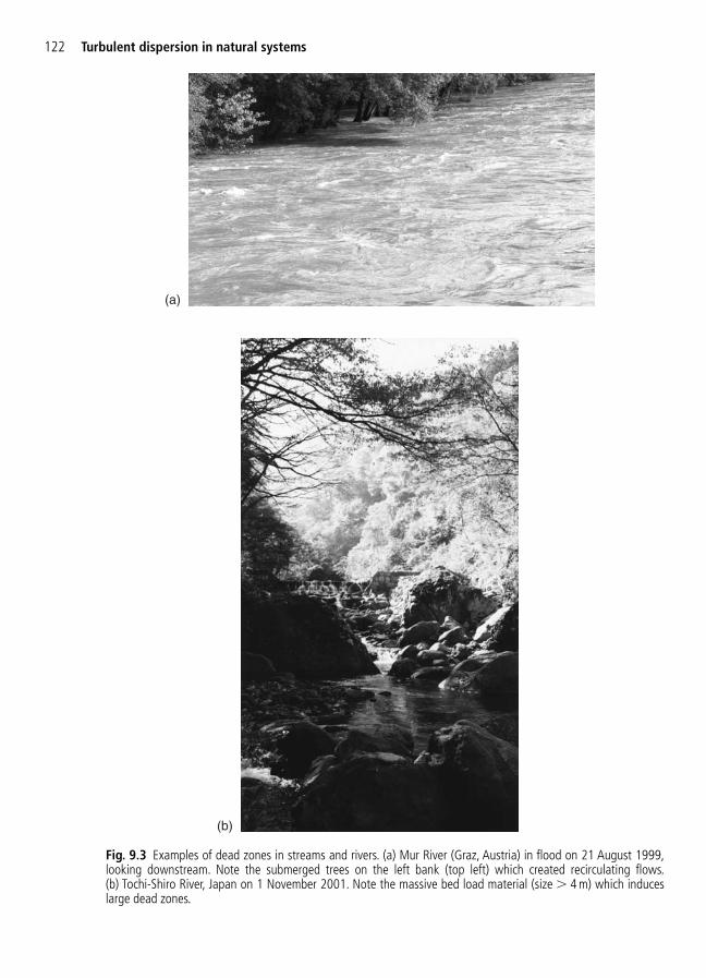
122 Turbulent dispersion in natural systems

(a)

Fig. 9.3 Examples of dead zones in streams and rivers. (a) Mur River (Graz, Austria) in flood on 21 August 1999,looking downstream. Note the submerged trees on the left bank (top left) which created recirculating flows.(b) Tochi-Shiro River, Japan on 1 November 2001. Note the massive bed load material (size � 4 m) which induceslarge dead zones.

(b)

9.2 Longitudinal dispersion in natural rivers with dead zones 123

(c)

(d)

Fig. 9.3 (Contd ) (c) Small dead zone during the flood of the Seine River at Caudebec-en-Caux, France on 12 March2001 (courtesy of Ms Nathalie Lemiere, Sequana-Normandie). View from the right bank. The photograph was taken inthe afternoon at high tide. Spring tides (coefficient: 113 and tidal range: 8.5 m on 12/3/2001) induced significant back-water effect. (d) River restoration test section, looking upstream on 30 March 1999, ARRC River habitat research cen-tre, Gifu, Japan.The rectangular pond (i.e. dead zone) was designed to facilitate habitat restoration (see also Fig. 9.3(e)).(e) River restoration test section, looking downstream on 30 March 1999, ARRC River habitat research centre. This isa different type of river restoration system, compared to Fig. 9.3(d).

(e)

124 Turbulent dispersion in natural systems

Notes1. Dead zones increase the length of the initial zone and the longitudinal dispersion

coefficient.2. The length of the initial zone (i.e. advective zone) is the distance for complete mix-

ing from a centreline or side discharge (Chapters 7 and 8). In the presence of deadzones, the initial zone may be enlarged significantly, although there are differentinterpretations (e.g. Fischer et al. 1979, Rutherford 1994).

3. Equation (8.8) may underestimate dispersion coefficients in river systems with deadzones by a factor of 2–10, or even more. Relevant discussions include Valentine andWood (1979a, b) and Rutherford (1994, p. 202).

9.2.2 Basic equation

A river reach is modelled by a sequence of sub-reaches, or cells, which flows into each other.A simplified dead zone model may be developed assuming that:

1. each cell is well mixed,2. the outflow concentration equals the cell concentration (Fig. 9.2(b)),3. the inflow concentration equals the outflow concentration of the upstream cell, but with a

time delay �t.

Considering a non-conservative contaminant (decay rate k), the mass balance equation in acell {i} is:

(9.7)

where Vol is the cell volume, Q is the river discharge, C m{i} is the average contaminant con-

centration in cell {i} and k is the first-order decay rate coefficient (Section 9.3).

Vol( )

( Vol ( ){ } mm m

ii

i i iC tt

QC t t Q k C t∂

∂

{ }{ } { } { }( ) )� � � �1 �

Remarks1. There are basically three models of longitudinal dispersion with dead zone: the tran-

sient storage model, the cells in series (CIS) model and the ADZ model (Rutherford1994, pp. 218–229). The above development is the basic equation of the ADZ modelfirst introduced by Beer and Young (1983). The present form derives from the workof Wallis et al. (1989). Rutherford recommended the ADZ model, although hewarned of the lack of physical meaning of the ADZ model coefficients.

2. The dispersion and transport of reactive contaminants are discussed in Sections 9.3and 9.4, where values of the decay rate constant are introduced.

9.2.3 Analytical solutions (instantaneous mass slug injection)

Considering the instantaneous injection of a mass slug M at t � 0 in the first sub-reach(i � 0), the solution of equation (9.7) for that cell (i.e. i � 0) is:

(9.8)C tM

t t t tm ( ) Vol

( for � � � � �exp ( ))� �

where � � k 1/�T and �T � Vol/Q is the cell residence time. Note that Cm(t � 0) �M/Vol: i.e. an instantaneous dilution.

For a two-cell system (Fig. 9.2(c)), the solution of equation (9.7) for the second cell (i � 1) is:

(9.9a)

Equation (9.9a) is the analytical solution for the second cell.Considering an instantaneous mass slug injection of mass M at t � 0 in the initial sub-

reach (i � 0) of a river system made of (n 1) identical sub-reaches, placed in series, thecontaminant concentration in the last cell (i.e. i � n) is:

(9.9b)

where n! is the n-factorial: n! � 1 � 2 � 3 � … � n.Equation (9.9) is plotted in Fig. 9.4 for a conservative contaminant (i.e. k � 0) and a

decaying substance (i.e. k � 0.003), and for two values of n. Note that the number of cells isdirectly related to the distance downstream. With increasing value of n, the time of passageof centroid increases and the peak concentration decreases. Qualitatively this trend is consist-ent with Taylor’s dispersion model for the sudden injection of a mass slug of contaminant(e.g. Fig. 8.3). For small values of n (e.g. n � 5), the concentration versus time distributionis skewed, while it becomes more symmetrical for larger values of n (e.g. n � 20).

C tt t

n

Mt t n

n n

m ( )

Vol( )) ( 1)-cell system�

�� �

��

��

( )!

exp(

C t t tM

t tm ( ) )Vol

( )) Two-cell system� � � � �� �( exp( �

9.2 Longitudinal dispersion in natural rivers with dead zones 125

Remarks1. For an instantaneous mass slug injection of mass M at t � 0 in two-cell river model,

the time of passage of the centroid in the second cell is:

2. For an instantaneous mass slug injection of mass M at t � 0 in a river system madeof (n 1) identical cells placed in series, the time of passage of the centroid T in thelast cell (i � n 1) equals:

3. In practice, the ADZ ‘dead zone’ model is best applied to predict the longitudinal dis-persion between two sites located both downstream of an injection point. The con-centration versus time distribution at the upstream site is divided as a succession ofsmall mass slugs as illustrated in Fig. 8.4. The final solution is obtained by applyingthe method of superposition.

4. Remember that, for an instantaneous mass slug injection in a two-cell model, themass of contaminant M is instantaneously diluted into the initial cell volume (i � 0)(Fig. 9.2(c)). Then it decays with time in the initial cell according to:

(9.8)C tM

t t im ( ) Vol

)) Initial cell ( 0)� � � �exp( (� �

T n T t )� (� �

T T t � � �

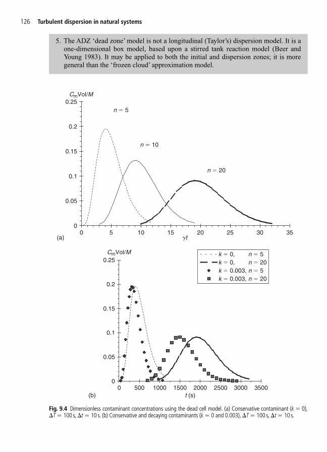
126 Turbulent dispersion in natural systems

(a)

0

0.05

0.1

0.15

0.2

0.25

0 5 10 15 20 25 30 35

CmVol/M

n � 5

n � 20

n � 10

gt

k � 0, n � 5k � 0, n � 20k � 0.003, n � 5k � 0.003, n � 20

0

0.05

0.1

0.15

0.2

0.25

0 500 1000 1500 2000 2500 3000 3500

CmVol/M

t (s)(b)

Fig. 9.4 Dimensionless contaminant concentrations using the dead cell model. (a) Conservative contaminant (k � 0),�T � 100 s, �t � 10 s. (b) Conservative and decaying contaminants (k � 0 and 0.003), �T � 100 s, �t � 10 s.

5. The ADZ ‘dead zone’ model is not a longitudinal (Taylor’s) dispersion model. It is aone-dimensional box model, based upon a stirred tank reaction model (Beer andYoung 1983). It may be applied to both the initial and dispersion zones; it is moregeneral than the ‘frozen cloud’ approximation model.

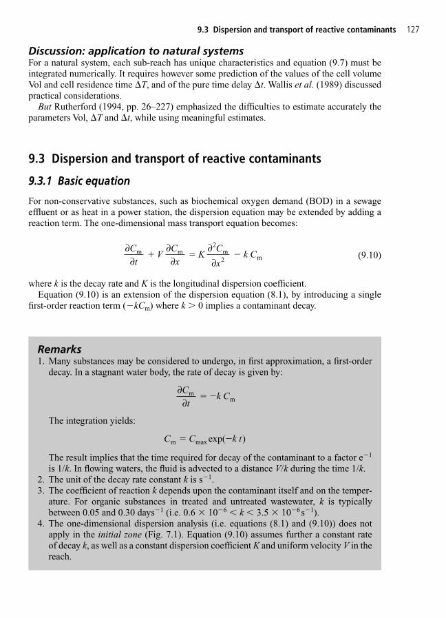
Discussion: application to natural systemsFor a natural system, each sub-reach has unique characteristics and equation (9.7) must beintegrated numerically. It requires however some prediction of the values of the cell volumeVol and cell residence time �T, and of the pure time delay �t. Wallis et al. (1989) discussedpractical considerations.

But Rutherford (1994, pp. 26–227) emphasized the difficulties to estimate accurately theparameters Vol, �T and �t, while using meaningful estimates.

9.3 Dispersion and transport of reactive contaminants

9.3.1 Basic equation

For non-conservative substances, such as biochemical oxygen demand (BOD) in a sewageeffluent or as heat in a power station, the dispersion equation may be extended by adding areaction term. The one-dimensional mass transport equation becomes:

(9.10)

where k is the decay rate and K is the longitudinal dispersion coefficient.Equation (9.10) is an extension of the dispersion equation (8.1), by introducing a single

first-order reaction term (�kCm) where k � 0 implies a contaminant decay.

∂∂

∂∂

∂∂

Ct

VCx

KC

xk Cm m m

m � �2

2

9.3 Dispersion and transport of reactive contaminants 127

Remarks1. Many substances may be considered to undergo, in first approximation, a first-order

decay. In a stagnant water body, the rate of decay is given by:

The integration yields:

The result implies that the time required for decay of the contaminant to a factor e�1

is 1/k. In flowing waters, the fluid is advected to a distance V/k during the time 1/k.2. The unit of the decay rate constant k is s�1.3. The coefficient of reaction k depends upon the contaminant itself and on the temper-

ature. For organic substances in treated and untreated wastewater, k is typicallybetween 0.05 and 0.30 days�1 (i.e. 0.6 � 10�6 � k � 3.5 � 10�6s�1).

4. The one-dimensional dispersion analysis (i.e. equations (8.1) and (9.10)) does notapply in the initial zone (Fig. 7.1). Equation (9.10) assumes further a constant rate of decay k, as well as a constant dispersion coefficient K and uniform velocity V in thereach.

C C k tm max )� �exp(

∂∂C

tk Cm

m � �

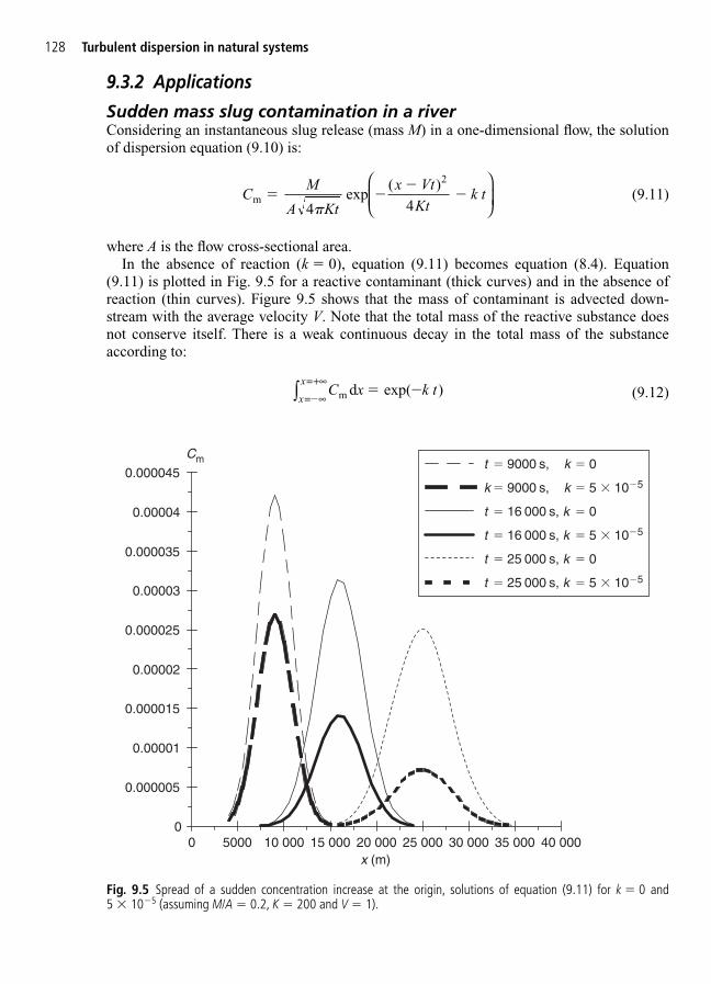
9.3.2 Applications

Sudden mass slug contamination in a riverConsidering an instantaneous slug release (mass M) in a one-dimensional flow, the solutionof dispersion equation (9.10) is:

(9.11)

where A is the flow cross-sectional area.In the absence of reaction (k � 0), equation (9.11) becomes equation (8.4). Equation

(9.11) is plotted in Fig. 9.5 for a reactive contaminant (thick curves) and in the absence ofreaction (thin curves). Figure 9.5 shows that the mass of contaminant is advected down-stream with the average velocity V. Note that the total mass of the reactive substance does not conserve itself. There is a weak continuous decay in the total mass of the substanceaccording to:

(9.12)C x k tx

xm d

= ∞

=+∞∫ �

� �exp( )

CM

A Kt

x VtKt

k tm

� ��

�4 4

2

�exp

( )

128 Turbulent dispersion in natural systems

t � 9000 s, k � 0

t � 16 000 s, k � 5 � 10�5

k � 9000 s, k � 5 � 10�5

t � 25 000 s, k � 0

t � 16 000 s, k � 0

t � 25 000 s, k � 5 � 10�5

0

0.000005

0.00001

0.000015

0.00002

0.000025

0.00003

0.000035

0.00004

0.000045

0 5000 10 000 15 000 20 000 25 000 30 000 35 000 40 000

Cm

x (m)

Fig. 9.5 Spread of a sudden concentration increase at the origin, solutions of equation (9.11) for k � 0 and5 � 10�5 (assuming M/A � 0.2, K � 200 and V � 1).

Sudden increase in mass concentration at the originThe concentration is initially zero everywhere. At the initial time t � 0, the concentration issuddenly raised to Co at the origin x � 0 and held constant: Cm(0, t � 0) � Co. This is asteady situation and the dispersion equation becomes:

(9.13)

with the boundary condition: Cm � 0 at x � �. A solution of the dispersion equation is:

(9.14a)

where:

and Co is an integration constant. Neglecting the existence of the initial zone, the initial con-centration Co is equivalent to the steady release of M

.units of mass per unit time into a river

(discharge Q):

(9.15)CMQo � �˙ 2

1 1�

�( )

� = 42

K k

V

C Ck xVm o

� � �exp2

1 1�

�( )

VCx

KC

xkC

∂∂

∂∂

m mm � �

2

2

9.3 Dispersion and transport of reactive contaminants 129

Remarks1. At a distance x from the injection point, the maximum mass concentration equals:

The result leads to equation (8.7) for k � 0 (no reaction).2. The standard deviation of the contaminant cloud equals: . � 2Kt

CM

A KxV

kxVmax

� �

4�

exp

Remarks1. � � 4Kk/V2 is a dimensionless coefficient of reaction–dispersion. For BOD, � is typ-

ically of the order: � � 0.4.2. In natural rivers and using equations (7.6) and (8.8), it yields:

where W is the channel width and �t is the transverse mixing coefficient.

�

2

2

t

� ��

40 0264

K k

V

W k.

9.3.3 Discussion

The one-dimensional dispersion analysis (equation (9.10)) assumes that the contaminant isfully mixed across the channel: i.e. it does not apply to the initial zone (Fig. 7.1). For a steadyflow in rivers, the distance required for cross-sectional mixing is about (Section 5.3):

while the characteristic distance of contaminant decay is V/k.1 The latter exceeds the cross-sectional mixing distance (i.e. x� � 0.4) only if the dimensionless coefficient of reaction–dispersion � is less than about 0.066.

If the contaminant concentration decays before the end of the initial zone (i.e. x� � 0.4),equation (9.10) is not suitable, and the contaminant concentration must be computed numer-ically (e.g. Fischer et al. 1979). Practically, equation (9.10) may be applied only for � � 0.066.

If the longitudinal dispersion term is very small (i.e. K ∂2Cm / ∂2x �� kCm), the dimension-less coefficient of reaction–dispersion � is very small. Considering a steady river flow andcontaminant injection, the solution of equation (9.13) becomes:

(9.14b)

Equation (9.14b) is a reasonable prediction of the downstream contaminant concentration forvery small values of �.

C Ck xVm o

for very small� �exp

�

L V W Complete mixing of side discharge2t� 0 4. /�

130 Turbulent dispersion in natural systems

Remarks1. Fischer et al. (1979, p. 147) stated that � � 0.06 for the decay distance to be greater than

the length of the initial zone. The above result (i.e. � � 0.066) is more precise, althoughit must be emphasized that equations (7.6) and (8.8) are approximate (Chapters 7 and 8).

2. For small values of �, the longitudinal dispersion term in equation (9.10) is verysmall (i.e. K ∂2Cm / ∂x2 �� kCm).

3. In practice, effluent discharges are rarely steady. Typical daily fluctuations in sewageoutput lead to gradients of concentration of the discharged material, and these gradi-ents are subsequently smoothed by the process of longitudinal dispersion. Henceequations (9.14a) and (9.14b) are seldom applicable.

9.4 Transport with reaction

9.4.1 Basic equation

A particular case is the transport of reactive contaminant from a continuous source at origin,under steady flow conditions, and in the absence of longitudinal dispersion. That is, the dispersion term in equation (9.10) is assumed negligible:

KC

x

∂∂

2

20m �

1Remember that the time required for decay of the contaminant to a factor e�1 is 1/k, during which the fluid isadvected to a distance V/k.

For steady flow conditions, the dispersion equation becomes:

(9.16)

where kr is the decay rate constant (s�1). The integration of the transport equation (9.16)yields:

(9.17)

where Co � M.

/Q, M.

is the mass flow rate of contaminant at x � 0 and Q is the steady riverdischarge.

9.4.2 Application to dissolved oxygen content (DOC) in natural streams

Equation (9.16) may be applied to estimate the self-cleaning capacity of a waterway receiv-ing wastes. The water in the channel has the capacity to absorb organic matter and pollutants:i.e. through the micro-organisms that degrade certain non-conservative pollutants of organicorigin (e.g. wastewater).

In a waterway, the sources of dissolved oxygen (DO) are the re-oxygenation at the free sur-face and the photosynthesis. The sinks of oxygen include the biochemical oxygenation oforganic matter, the decomposition of sludge deposits and the respiration of aquatic plants andlife forms. In a first approximation, the budget of the DO is primarily a function of the re-oxygenation rate and the biochemical oxygenation demand (BOD) (Fig. 9.6). At steadystate, the DO balance may be expressed as:

(9.18)

where x is the distance in the flow direction, Cm is the DO concentration, BOD is the bio-chemical oxygen demand, Csat is the concentration of dissolved gas in water at equilibrium(Appendix B, Section 9.6), ka is the re-oxygenation rate constant and kr is the BOD decay rate.

VCx

k C C k∂∂

ma sat m r BOD� � �( )

C Ck xVm or � �exp

VCx

k C∂∂

mr m � �

9.4 Transport with reaction 131

Free-surfaceoxygenation

Biochemicaloxygenation

OrganicmatterDissolved oxygen

Fig. 9.6 Simplified analysis of DO balance in a waterway.

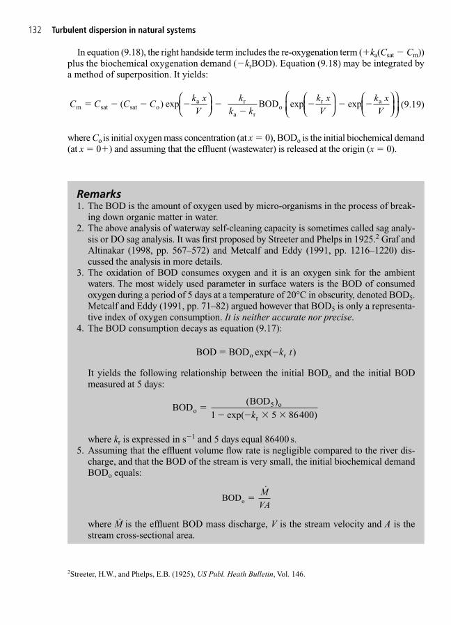
In equation (9.18), the right handside term includes the re-oxygenation term (ka(Csat � Cm))plus the biochemical oxygenation demand (�krBOD). Equation (9.18) may be integrated bya method of superposition. It yields:

(9.19)

where Co is initial oxygen mass concentration (at x � 0), BODo is the initial biochemical demand(at x � 0) and assuming that the effluent (wastewater) is released at the origin (x � 0).

C C C Ck xV

kk k

k xV

k xVm sat sat o

a r

a ro

r a (

BOD exp

� � � � ��

� � �) exp exp

132 Turbulent dispersion in natural systems

Remarks1. The BOD is the amount of oxygen used by micro-organisms in the process of break-

ing down organic matter in water.2. The above analysis of waterway self-cleaning capacity is sometimes called sag analy-

sis or DO sag analysis. It was first proposed by Streeter and Phelps in 1925.2 Graf andAltinakar (1998, pp. 567–572) and Metcalf and Eddy (1991, pp. 1216–1220) dis-cussed the analysis in more details.

3. The oxidation of BOD consumes oxygen and it is an oxygen sink for the ambientwaters. The most widely used parameter in surface waters is the BOD of consumedoxygen during a period of 5 days at a temperature of 20°C in obscurity, denoted BOD5.Metcalf and Eddy (1991, pp. 71–82) argued however that BOD5 is only a representa-tive index of oxygen consumption. It is neither accurate nor precise.

4. The BOD consumption decays as equation (9.17):

It yields the following relationship between the initial BODo and the initial BODmeasured at 5 days:

where kr is expressed in s�1 and 5 days equal 86400 s.5. Assuming that the effluent volume flow rate is negligible compared to the river dis-

charge, and that the BOD of the stream is very small, the initial biochemical demandBODo equals:

where M.

is the effluent BOD mass discharge, V is the stream velocity and A is thestream cross-sectional area.

BOD o �M

VA

BOD BOD

exp( oo

r

�� � � �

( ))

5

1 5 86400k

BOD BODo r� �exp( )k t

2Streeter, H.W., and Phelps, E.B. (1925), US Publ. Heath Bulletin, Vol. 146.

Re-oxygenation rate constant and decay rateTypical values of the decay rate constant of organic matter contained in wastewater are listedin Table 9.1. For the re-aeration rate constant, there are numerous correlations and Table 9.2summarizes some. Accurate estimates of concentration of dissolved gas in water at equilib-rium Csat and molecular diffusivity Dm are given in Appendices B and C.

While Table 9.1 provides accepted estimates of the decay rate constant for BOD, the calculations of the re-aeration rate constant are most often empirical and inaccurate. In prac-tice, the correlation of Gualtieri et al. (2002) may provide a robust estimate for clear-waterflows.

9.4 Transport with reaction 133

6. In the general case, the initial BOD equals:

where Qeffluent is the effluent volume flow rate, BOD (x � 0) is the BOD of the riverupstream of the effluent injection location and Q is the river flow rate.

BOD BOD

oeffluent

� �

˙ ( )M x QQ Q

0

Table 9.1 Typical BOD decay rate

Effluent kr (day�1) BODo (mg/L)(1) (2) (3)

Strong wastewater 0.39 250–400Weak wastewater 0.35 110–150Primary effluent 0.35 75–150Secondary effluent 0.12–0.23 15–75Tap water �0.12 �1

References: Fair et al. (1968), Barnes et al. (1981), Liu et al. (1997).

Table 9.2 Empirical correlations of re-aeration rate constant in open channels (neglecting ‘white waters’)

Reference ka Remarks(1) (2) (3)

Fair et al. (1968) ka in day�1, V in m/s and d in m

Gualtieri et al. (2002) Dimensionally correct relationship, ka in s�1; based upon a large number of USGS field experiments in natural streams�: kinematic viscosity: surface tension

Simplified expression Rough estimate based upon geometrical considerations and liquid film coefficient estimate (see Appendix A) ka in s�1; kL in m/s and d in m

Notes: Dm: molecular diffusivity (Appendix C, Section 9.7).

k

dL

1 12

2 3

5 33

3 4

33. sin

/

/

D

d

gm

���

� �

11 0.V

d5/3

9.4.3 DO sag analysis

Equation (9.19) is plotted in Fig. 9.7 for one particular example. The shape is typical.Downstream of the effluent injection (i.e. x � 0), the biochemical decomposition of the waste-water induces a reduction in DOC. However DO is replenished through surface aeration at arate proportional to the DO deficit (i.e. (Csat � Cm)). At a certain point, the re-aeration rateequals exactly the BOD consumption. Downstream, the aeration rate is larger than the BOD

134 Turbulent dispersion in natural systems

3In clear-water flows, a is the air–water interface area per unit volume of water. In turbulent air–water flows, a isthe air–water surface area per unit of (flowing) air and water.

Discussion: aeration rate constant in ‘white-water’ flowsThe re-oxygenation constant rate ka is the product of the liquid film coefficient kL by thespecific surface area:

where a is the air–water interface area per unit volume of flowing fluid.3 The liquid filmcoefficient is primarily a function of the fluid and gas properties only (Appendix C,Section 9.7).

In air–water flows (i.e. ‘white waters’), the re-oxygenation rate is drastically enhancedby the cumulative surface area of entrained bubbles (Appendix A and Fig. 9.8). Forexample, in a 2 m deep river with a depth-averaged specific interface area of 200 m2/m3,the re-aeration rate constant ka is 400 times greater than predicted by clear-water flowcorrelations shown in Table 9.2.

Remarks1. In natural channels, the re-aeration rate constant is enhanced by secondary currents

and surface renewal induced by large eddies. For example, Gulliver and Halverson(1989), Tamburrino and Gulliver (1990).

2. In bubbly air–water flows, the specific interface area equals:

where dab is the air bubble diameter and C is the void fraction (also called air con-centration). For example, a � 400 m�1 for C � 0.2 and dab � 3 mm.

3. The temperature influence on the aeration rate constant is often approximated by:

where T is the temperature in Celsius and ka(T � 20°C) is the reference aeration rateconstant at 20°C. However the influence of temperature must be properly accountedfor through the fluid properties (e.g. �, �, , Dm) which are temperature dependent.

4. Most aeration rate calculations neglect the effects of wind speed and cross-sectionalshape. The wind speed is little relevant in flowing waters. The cross-sectional shapehas little effect for wide channels.

k T k T Ta a( ) ( C � = ° −20 1 024 20) .

aCd

ab

� 6

k k aa L �

consumption and the DO content increases with distance. Far downstream, the watersbecomes more and less saturated in DO. This may occur at a large downstream distance.

Important parameters of the DO sag curve are the minimum DO concentration (Cm)min andthe distance Xmin where it takes place. These may be estimated from equation (9.19) for∂Cm/∂x � 0. It yields:

(9.20)

(9.21)( ) BOD expm minr

ao

r minCkk

k XV

� �

XV

k kkk

C C k k

kmina r

a

r

sat o a r

r o

ln

BOD�

��

� �

( )( )

1

9.4 Transport with reaction 135

0

0.001

0.002

0.003

0.004

0.005

0.006

0.007

0.008

0.009

0 20 000 40 000 60 000 80 000 100 000 120 000 140 000 160 000 180 000 200 000

Cm (kg/m3)

x (m)

at 20°C

Xmin

(Cm)min

Csat

Fig. 9.7 Evolution of DO concentration in streams downstream of effluent injection: BODo � 0.0198 kg/m3,Co � 0.080 kg/m3, Q � 38 m3/s, V � 0.22 m/s, d � 3.5 m, 20°C.

Remarks1. It is important to remember that the BOD consumption decays as equation (9.17),

while the re-aeration rate is proportional to the DO deficit (Csat � Cm).2. The time of arrival of the minimum DO content is tmin � Xmin/V.3. The ‘sag analysis’ has limited use because equations (9.18) and (9.19) neglect some

important phenomena. In particular, they neglect several sources and sinks of DO:e.g. photosynthesis and ‘white waters’, the decomposition of sludge deposits andrespiration of aquatic plants and life forms. Further equations (9.18)–(9.21) assumeconstant ka, kr, V and Q, and steady flow conditions.

9.5 Appendix A – Air–water mass transfer in air–water flows

Air–water flows in rivers and hydraulic structures have great potential for aeration enhance-ment of flow because of the large interfacial area generated by entrained bubbles (Part 4,Chapter 17; Chanson 1997, Fig. 7.8).

The mass transfer rate of a chemical across an interface varies directly as the coefficient ofmolecular diffusion and the negative gradient of gas concentration. If the chemical of inter-est is volatile (e.g. oxygen, nitrogen, chlorine, methane), the transfer is controlled by the liq-uid phase, and the gas transfer of the dissolved chemical across an air–water interface isusually rewritten as:

(9A.1)

where kL is the liquid film coefficient, a is the specific surface area defined as the air–waterinterface area per unit volume of air and water, Cm is the local dissolved gas concentrationand Csat is the concentration of dissolved gas in water at equilibrium (Appendix B) (e.g.Gulliver 1990, Chanson and Toombes 2000, Chanson 2002). Mass transfer at bubble inter-face is a complex process. Kawase and Moo-Young (1992) reviewed several correlations forthe liquid film coefficient calculations in turbulent gas–liquid flows. They showed that themass transfer coefficient kL is almost constant regardless of bubble sizes and flow situations.The transfer coefficient may be estimated by:

(9A.2a)

(9A.2b)

for gas bubbles affected by surface active impurities, where �w and �w are the dynamic viscos-ity and density of the liquid, Dgas is the coefficient of molecular diffusion (Appendix C, Section9.7), dab is the gas bubble diameter, g is the gravity acceleration, all variables being expressedin SI units. Equation (9A.2) was compared successfully with more than a dozen of experimen-tal studies.

Equation (9A.1) is very general. Importantly, it includes the effect of air bubble entrain-ment and the drastic increase in interfacial area. Experimental measurements in supercriticalflows down a flat chute recorded local specific interface area of up to 110 m2/m3 (m�1) withdepth-averaged (bulk) interface area ranging from 10 to 21 m�1. Larger specific interfaceareas were recorded in developing shear flows. Local interface areas of up to 400 m�1 wereobserved in hydraulic jumps and maximum specific interface areas of up to 550 m�1 (4) weremeasured in plunging jet flows (Chanson 1997, Chanson and Toombes 2000). These examplesillustrate the potential for aeration enhancement in the presence of white water.

Chanson and Toombes (2000) combined equations (9A.1) and (9A.2) with measuredair–water interfacial areas. They deduced aeration efficiency, in terms of DO, of about30–40% for a 24 m long stepped cascade with a 1.4 m total drop. The result was verified withDO measurements. The very large aeration rate derives from the strong flow aeration andsustained air–water interface areas down the entire chute (Fig. 9.8).

k D g dL gasw

w

1/6

3ab 0.25 mm� �

�

0 47.�

�

k D g dL gas2/3 w

wab 0.25 mm� �

�

0 281 3

3.�

�

∂∂C

tk a C Cm

L m sat )� � �(

136 Turbulent dispersion in natural systems

4That is, nearly twice the surface area of two basketball courts in one cubic metre of air and water.

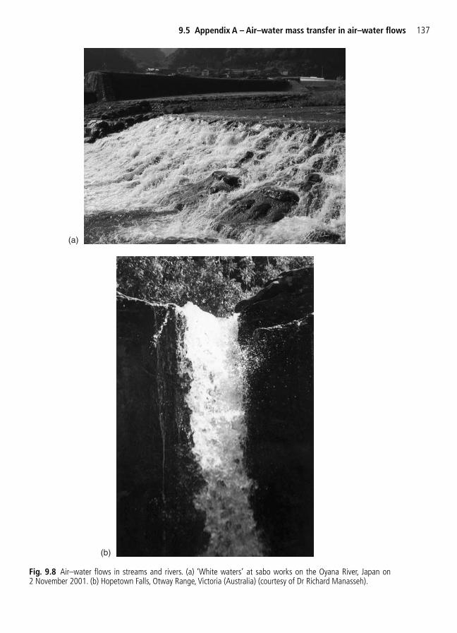
9.5 Appendix A – Air–water mass transfer in air–water flows 137

(b)

Fig. 9.8 Air–water flows in streams and rivers. (a) ‘White waters’ at sabo works on the Oyana River, Japan on 2 November 2001. (b) Hopetown Falls, Otway Range, Victoria (Australia) (courtesy of Dr Richard Manasseh).

(a)

9.6 Appendix B – Solubility of nitrogen, oxygen and argon in water

Dissolved gas concentrations in water are usually expressed in mass of dissolved chemicalper unit volume or kg/m3. Another unit is the ppm (parts per million). The conversion is:1 ppm � 1 mg/L.

Solubility of oxygenThe solubility of oxygen in water at equilibrium with water saturated air Csat(Pstd) at stand-ard pressure (i.e. Pstd � 1 atm � 1.013 25 � 105Pa) is calculated as:

where Csat (Pstd) is the solubility of oxygen at standard pressure5 in kg/m3, TK is the tem-perature in Kelvin and Chl is the chlorinity in ppt.6 The saturation concentration of DO atnon-standard pressure is:

(9B.2)

where P is the absolute pressure in atm (within 0–2 atm), Pv is the partial pressure of watervapour in atm and TK is the temperature in Kelvin. In equation (9B.2), the expression of Teta is:

(9B.3)

where TC is the temperature in Celsius. The partial pressure of water vapour may be com-puted as:

(9B.4)

where Pv is in atm.References: Apha (1985, 1989), Bowie et al. (1985).

ln( 3840.70

TK

216 961

TKv 2

P ) .� � �11 8571

Teta 1.426 10 TC 6.436 10 TC2� � � �� �0 000975 5 8.

C P C P

PP

P

Psat s

v

v

( (Pstd

Teta(

Teta) )

)

�

� �

� �

1 1

1 1

( )

( )( )

ln( ( ))

. . .

..

1000

6 642308 1 243800 0 8 621 949

3 192919 428

2

10

3 4

2

Csat

5

7 11

23

Pstd 139.344 11 1.575701 10

TK

10

TK

1

TK

10

TK

Chl 10 TK

3.8673 10

TK

� � �

��

�

��

� � � ��

138 Turbulent dispersion in natural systems

5The standard pressure Pstd (also called standard atmosphere or normal pressure) at sea level equals:

Pstd � 1 atm � 360 mm of Hg � 101 325 Pa

where Hg is the chemical symbol of mercury.6The chlorinity is defined in relation to salinity as: Salinity � 1.806 55 � Chlorinity.

(9B.1)

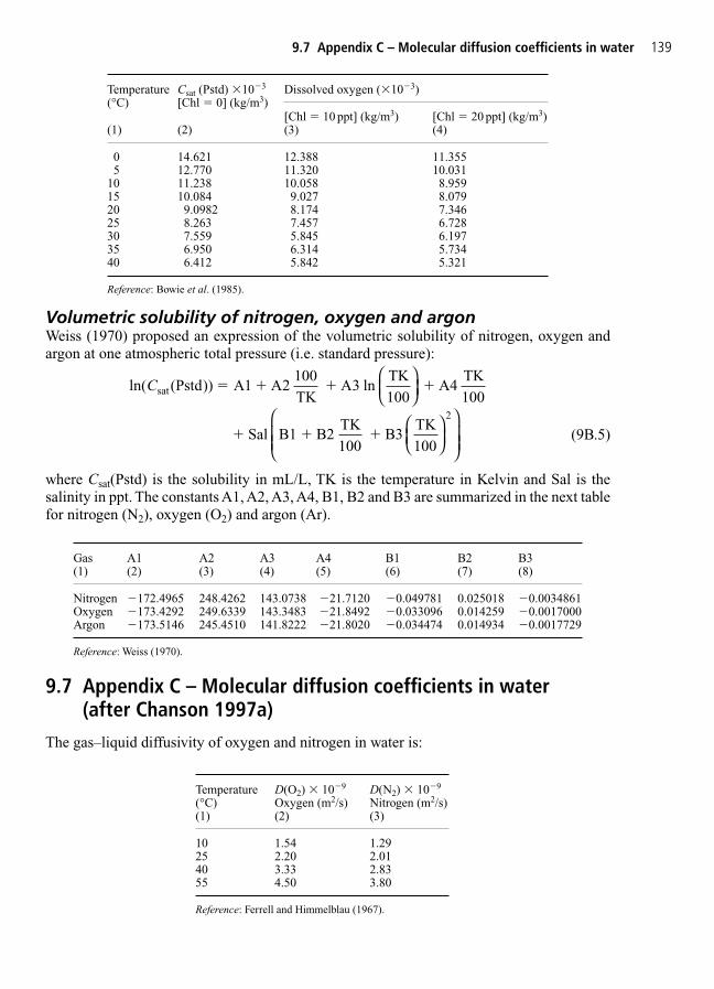
Volumetric solubility of nitrogen, oxygen and argonWeiss (1970) proposed an expression of the volumetric solubility of nitrogen, oxygen andargon at one atmospheric total pressure (i.e. standard pressure):

(9B.5)

where Csat(Pstd) is the solubility in mL/L, TK is the temperature in Kelvin and Sal is thesalinity in ppt. The constants A1, A2, A3, A4, B1, B2 and B3 are summarized in the next tablefor nitrogen (N2), oxygen (O2) and argon (Ar).

ln (Pstd A ATK

ATK

A4TK100

Sal B1 B2TK100

B3TK100

sat( )) lnC �

1 2100

3100

2

9.7 Appendix C – Molecular diffusion coefficients in water 139

Temperature Csat (Pstd) �10�3 Dissolved oxygen (�10�3)(°C) [Chl � 0] (kg/m3)

[Chl � 10 ppt] (kg/m3) [Chl � 20 ppt] (kg/m3)(1) (2) (3) (4)

0 14.621 12.388 11.3555 12.770 11.320 10.031

10 11.238 10.058 8.95915 10.084 9.027 8.07920 9.0982 8.174 7.34625 8.263 7.457 6.72830 7.559 5.845 6.19735 6.950 6.314 5.73440 6.412 5.842 5.321

Reference: Bowie et al. (1985).

Gas A1 A2 A3 A4 B1 B2 B3(1) (2) (3) (4) (5) (6) (7) (8)

Nitrogen �172.4965 248.4262 143.0738 �21.7120 �0.049781 0.025018 �0.0034861Oxygen �173.4292 249.6339 143.3483 �21.8492 �0.033096 0.014259 �0.0017000Argon �173.5146 245.4510 141.8222 �21.8020 �0.034474 0.014934 �0.0017729

Reference: Weiss (1970).

9.7 Appendix C – Molecular diffusion coefficients in water (after Chanson 1997a)

The gas–liquid diffusivity of oxygen and nitrogen in water is:

Temperature D(O2) � 10�9 D(N2) � 10�9

(°C) Oxygen (m2/s) Nitrogen (m2/s)(1) (2) (3)

10 1.54 1.2925 2.20 2.0140 3.33 2.8355 4.50 3.80

Reference: Ferrell and Himmelblau (1967).

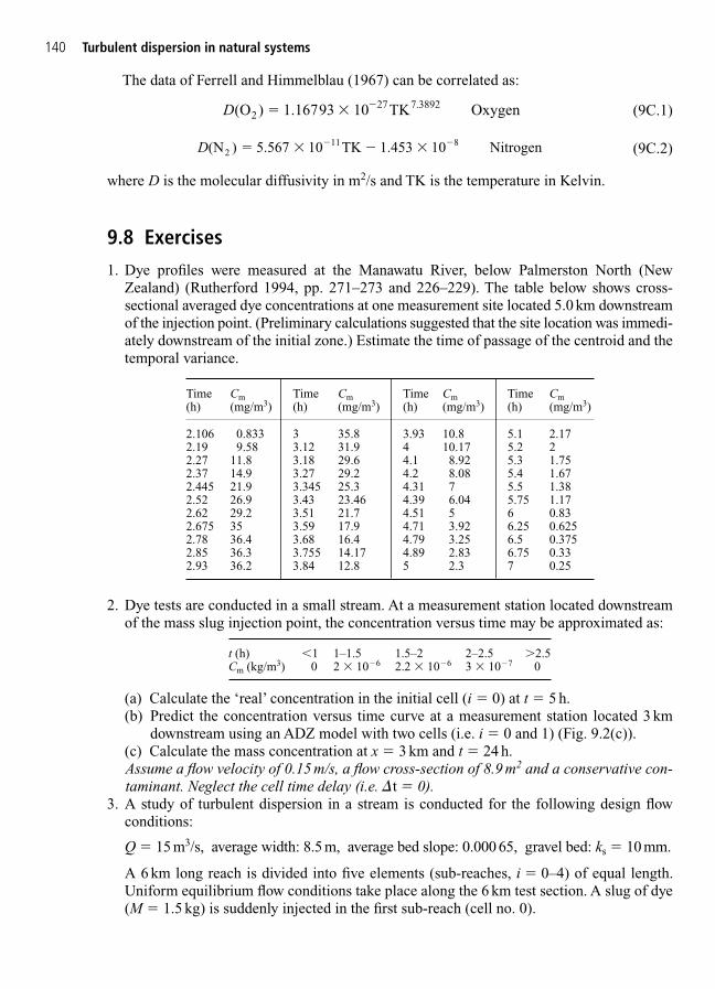
140 Turbulent dispersion in natural systems

The data of Ferrell and Himmelblau (1967) can be correlated as:

(9C.1)

(9C.2)

where D is the molecular diffusivity in m2/s and TK is the temperature in Kelvin.

9.8 Exercises

1. Dye profiles were measured at the Manawatu River, below Palmerston North (NewZealand) (Rutherford 1994, pp. 271–273 and 226–229). The table below shows cross-sectional averaged dye concentrations at one measurement site located 5.0 km downstreamof the injection point. (Preliminary calculations suggested that the site location was immedi-ately downstream of the initial zone.) Estimate the time of passage of the centroid and thetemporal variance.

D(N 10 TK 1.453 10 Nitrogen2 ) .� � � �� �5 567 11 8

D(O 1 1 10 TK Oxygen2 ) . .� � �6793 27 7 3892

2. Dye tests are conducted in a small stream. At a measurement station located downstreamof the mass slug injection point, the concentration versus time may be approximated as:

(a) Calculate the ‘real’ concentration in the initial cell (i � 0) at t � 5 h.(b) Predict the concentration versus time curve at a measurement station located 3 km

downstream using an ADZ model with two cells (i.e. i � 0 and 1) (Fig. 9.2(c)).(c) Calculate the mass concentration at x � 3 km and t � 24 h.Assume a flow velocity of 0.15 m/s, a flow cross-section of 8.9 m2 and a conservative con-taminant. Neglect the cell time delay (i.e. �t � 0).

3. A study of turbulent dispersion in a stream is conducted for the following design flow conditions:

Q � 15 m3/s, average width: 8.5 m, average bed slope: 0.000 65, gravel bed: ks � 10 mm.

A 6 km long reach is divided into five elements (sub-reaches, i � 0–4) of equal length.Uniform equilibrium flow conditions take place along the 6 km test section. A slug of dye(M � 1.5 kg) is suddenly injected in the first sub-reach (cell no. 0).

Time Cm Time Cm Time Cm Time Cm(h) (mg/m3) (h) (mg/m3) (h) (mg/m3) (h) (mg/m3)

2.106 0.833 3 35.8 3.93 10.8 5.1 2.172.19 9.58 3.12 31.9 4 10.17 5.2 22.27 11.8 3.18 29.6 4.1 8.92 5.3 1.752.37 14.9 3.27 29.2 4.2 8.08 5.4 1.672.445 21.9 3.345 25.3 4.31 7 5.5 1.382.52 26.9 3.43 23.46 4.39 6.04 5.75 1.172.62 29.2 3.51 21.7 4.51 5 6 0.832.675 35 3.59 17.9 4.71 3.92 6.25 0.6252.78 36.4 3.68 16.4 4.79 3.25 6.5 0.3752.85 36.3 3.755 14.17 4.89 2.83 6.75 0.332.93 36.2 3.84 12.8 5 2.3 7 0.25

t (h) �1 1–1.5 1.5–2 2–2.5 �2.5Cm (kg/m3) 0 2 � 10�6 2.2 � 10�6 3 � 10�7 0

(a) Calculate the mass concentration versus time 6 km downstream of the injection point.(Neglect the initial zone. Discuss the approximation.)

(b) Calculate the mass concentration versus time in the cell no. 4 neglecting the cell timedelay (i.e. �t � 0).

(c) Calculate the mass concentration versus time in the cell no. 4 assuming �t � 20 min.Present your results on the same graph and discuss the differences.

4. A mass slug of dye tracer (7.5 kg) is released during a small flood in Norman Creek, onthe channel centreline from a foot bridge, to estimate the longitudinal dispersion coeffi-cient. The stream, in Southern Brisbane, has the following channel characteristics duringthe flood event:

Flow depth: 0.73 m, width: 55 m, bed slope: 0.002, short grass: ks � 3 mm.

(a) Calculate the maximum tracer concentration and its arrival time 13 500 m downstreamof the injection point assuming a conservative tracer.

(b) The wrong tracer was selected and found to be reactive (decay rate constant:0.8 day�1). At 13.5 km downstream of the injection point, calculate the maximumtracer concentration and the mass concentration at t � 1 h after injection.

Assume uniform equilibrium flow conditions. Neglect vertical mixing and assume a slowlymeandering stream.

5. During the same flood event, in Norman Creek (Exercise 4), a reactive contaminant is accidentally released from the channel centreline as a mass slug. The decay rate con-stant is 400 day�1. May you use the longitudinal dispersion theory? In the affirmative, calculate the maximum tracer concentration at 3.5 km downstream of the injection point(slug mass: 1 kg).

6. A stream flows with an average velocity of 1 m/s and a flow rate of 8.5 m3/s. The water is95% saturated in DO and the water temperature is 10°C. The BOD5 is 0.001 kg/m3. Awater treatment plant discharge some effluent into the stream at a rate of 1.5 m3/s and theBOD5 is 200 g/m3. The decay rate constant and the re-aeration rate constant were previ-ously estimated to be 0.2 and 0.5 day�1 respectively.

Calculate the minimum DOC downstream of the injection point and its location.Estimate the BOD5 for a sample taken at that location. Assume the effluent to be at thesame temperature as the river. Assume further that the wastewater spreads almost instan-taneously across the entire section.

9.9 Exercise solutions

1. Manawatu River.Time of passage of the centroid � 3 h 17 min 30 s Temporal variance � 1.47 �108s2.

2. The problem is solved by assuming that the concentration distribution at the upstream sitecorresponds to the superposition of three mass slugs:

9.9 Exercise solutions 141

M (kg) 2 � 10�6 � 3000 � 8.9 2.2 � 10�6 � 3000 � 8.9 3 � 10�7 � 3000 � 8.9T (s) 4500 (1.25 h) 6300 8100

The volume of each cell is 3000 m � 8.9 m2. The cell residence time is �T �26 700/(0.15 � 8.9) � 20 000 s.

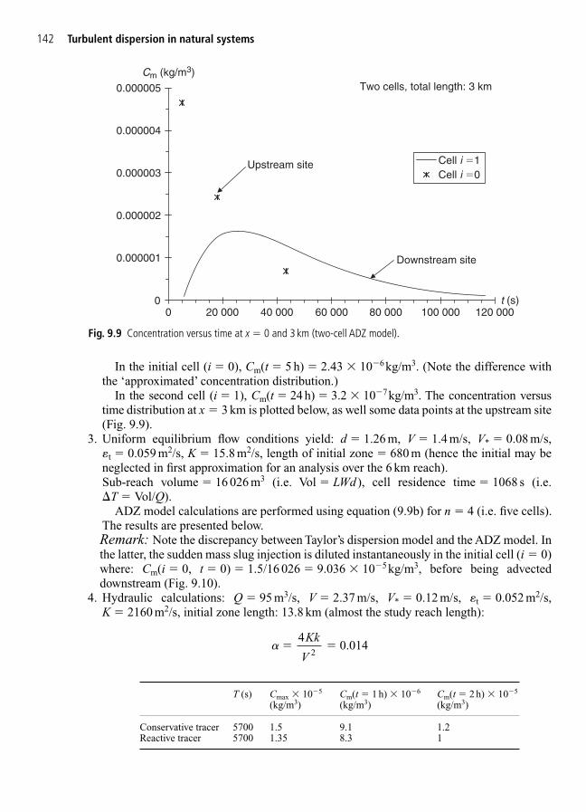
142 Turbulent dispersion in natural systems

In the initial cell (i � 0), Cm(t � 5 h) � 2.43 � 10�6kg/m3. (Note the difference withthe ‘approximated’ concentration distribution.)

In the second cell (i � 1), Cm(t � 24 h) � 3.2 � 10�7kg/m3. The concentration versustime distribution at x � 3 km is plotted below, as well some data points at the upstream site(Fig. 9.9).

3. Uniform equilibrium flow conditions yield: d � 1.26 m, V � 1.4 m/s, V* � 0.08 m/s,�t � 0.059 m2/s, K � 15.8 m2/s, length of initial zone � 680 m (hence the initial may beneglected in first approximation for an analysis over the 6 km reach).Sub-reach volume � 16 026 m3 (i.e. Vol � LWd), cell residence time � 1068 s (i.e.�T � Vol/Q).

ADZ model calculations are performed using equation (9.9b) for n � 4 (i.e. five cells).The results are presented below.Remark: Note the discrepancy between Taylor’s dispersion model and the ADZ model. Inthe latter, the sudden mass slug injection is diluted instantaneously in the initial cell (i � 0)where: Cm(i � 0, t � 0) � 1.5/16 026 � 9.036 � 10�5kg/m3, before being advecteddownstream (Fig. 9.10).

4. Hydraulic calculations: Q � 95 m3/s, V � 2.37 m/s, V* � 0.12 m/s, �t � 0.052 m2/s,K � 2160 m2/s, initial zone length: 13.8 km (almost the study reach length):

� 2

� �4

0 014Kk

V.

0

0.000001

0.000002

0.000003

0.000004

0.000005

0 20 000 40 000 60 000 80 000 100 000 120 000

Cell i �1Cell i �0

t (s)

Cm (kg/m3)Two cells, total length: 3 km

Upstream site

Downstream site

Fig. 9.9 Concentration versus time at x � 0 and 3 km (two-cell ADZ model).

T (s) Cmax � 10�5 Cm(t � 1 h) � 10�6 Cm(t � 2 h) � 10�5

(kg/m3) (kg/m3) (kg/m3)

Conservative tracer 5700 1.5 9.1 1.2Reactive tracer 5700 1.35 8.3 1

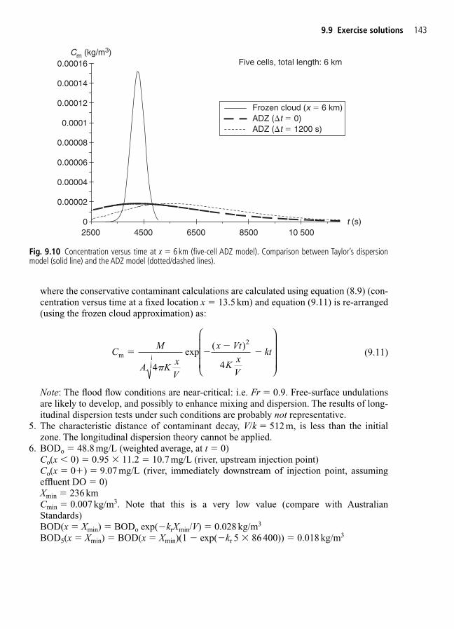
where the conservative contaminant calculations are calculated using equation (8.9) (con-centration versus time at a fixed location x � 13.5 km) and equation (9.11) is re-arranged(using the frozen cloud approximation) as:

(9.11)

Note: The flood flow conditions are near-critical: i.e. Fr � 0.9. Free-surface undulationsare likely to develop, and possibly to enhance mixing and dispersion. The results of long-itudinal dispersion tests under such conditions are probably not representative.

5. The characteristic distance of contaminant decay, V/k � 512 m, is less than the initialzone. The longitudinal dispersion theory cannot be applied.

6. BODo � 48.8 mg/L (weighted average, at t � 0)Co(x � 0) � 0.95 � 11.2 � 10.7 mg/L (river, upstream injection point)Co(x � 0) � 9.07 mg/L (river, immediately downstream of injection point, assumingeffluent DO � 0)Xmin � 236 kmCmin � 0.007 kg/m3. Note that this is a very low value (compare with AustralianStandards)BOD(x � Xmin) � BODo exp(�krXmin/V) � 0.028 kg/m3

BOD5(x � Xmin) � BOD(x � Xmin)(1 � exp(�kr 5 � 86 400)) � 0.018 kg/m3

CM

A KxV

x Vt

KxV

ktm (

� ��

�

4 4

2

�

exp)

9.9 Exercise solutions 143

0

0.00002

0.00004

0.00006

0.00008

0.0001

0.00012

0.00014

0.00016

2500 4500 6500 8500 10 500

Frozen cloud (x � 6 km)ADZ (�t � 0)ADZ (�t � 1200 s)

t (s)

Cm (kg/m3)Five cells, total length: 6 km

Fig. 9.10 Concentration versus time at x � 6 km (five-cell ADZ model). Comparison between Taylor’s dispersionmodel (solid line) and the ADZ model (dotted/dashed lines).

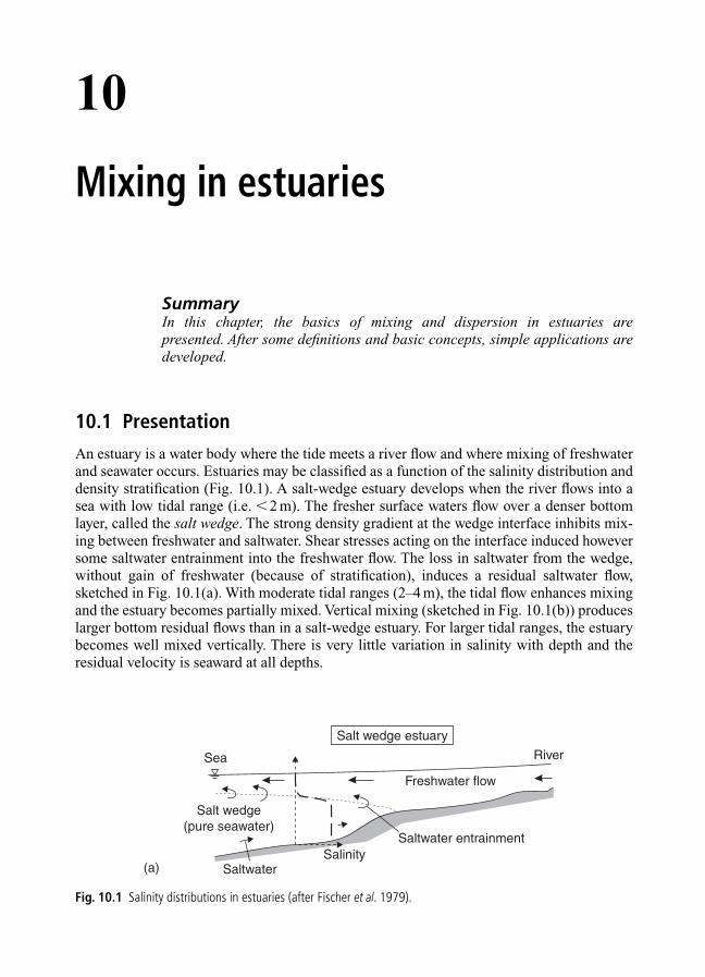
10

Mixing in estuaries

SummaryIn this chapter, the basics of mixing and dispersion in estuaries are presented. After some definitions and basic concepts, simple applications aredeveloped.

10.1 Presentation

An estuary is a water body where the tide meets a river flow and where mixing of freshwaterand seawater occurs. Estuaries may be classified as a function of the salinity distribution anddensity stratification (Fig. 10.1). A salt-wedge estuary develops when the river flows into asea with low tidal range (i.e. �2 m). The fresher surface waters flow over a denser bottomlayer, called the salt wedge. The strong density gradient at the wedge interface inhibits mix-ing between freshwater and saltwater. Shear stresses acting on the interface induced howeversome saltwater entrainment into the freshwater flow. The loss in saltwater from the wedge,without gain of freshwater (because of stratification), induces a residual saltwater flow,sketched in Fig. 10.1(a). With moderate tidal ranges (2–4 m), the tidal flow enhances mixingand the estuary becomes partially mixed. Vertical mixing (sketched in Fig. 10.1(b)) produceslarger bottom residual flows than in a salt-wedge estuary. For larger tidal ranges, the estuarybecomes well mixed vertically. There is very little variation in salinity with depth and theresidual velocity is seaward at all depths.

RiverSea

Freshwater flow

Salt wedge(pure seawater)

Salt wedge estuary

SalinitySaltwater entrainment

Saltwater(a)

Fig. 10.1 Salinity distributions in estuaries (after Fischer et al. 1979).

RiverSea

Salinity

SalinitySalinity

Vertically homogeneous estuary

RiverSea

Salinity

Salinity

Saltwater(b)

(c)

Partially mixed estuary

(a)

Fig. 10.1 (Contd )

Fig. 10.2 Examples of estuaries. (a) Estuary of the Columbia River, USA (courtesy of the Coastal and HydraulicsLaboratory, U.S. Army Corps of Engineers).

The above classification does not express the unique features of each estuary (Fig. 10.2),and it does not account for seasonal changes, nor for differences between neap and springtides. The study of mixing in estuary remains a complex process (Ippen 1966, Fischer et al.1979, Lewis 1997).

10.1 Presentation 145

146 Mixing in estuaries

(b-i)

Fig. 10.2 (Contd ) (b) Estuary of the Flora River, Dahouet (Côtes d’Armor, France) – looking upstream. The fjord-likeestuary is an harbour for fishing boats and small ships.A new marina was installed in the old swamp (background). Theriver arrives on the top left of the photograph.The tidal range may exceed 11 m in spring tides and the harbour is emptyat low tides. The estuary is well mixed. (b-i) At low tide on 8 September 2000. (b-ii) At high tide on 3 September 2000.

(b-ii)

10.1 Presentation 147

(c)

Fig. 10.2 (c) Hamanako Lake, Hama-matsu (Japan). Old sketch around AD 1707 (?) of Arai Check point (on left) andHamanako Lake Estuary.The Pacific Ocean is in the bottom foreground.Tidal range �2 m. (d) Permanently open BreeEstuary, South Africa (courtesy of the CERM, South Africa). Western Cape Estuary.

(d)

148 Mixing in estuaries

(e)

(f)

Fig. 10.2 (Contd ) (e) Permanently open Sundays River Estuary in the Eastern Cape, South Africa (courtesy of theCERM, South Africa). The photograph shows the extensive flood tidal delta inside the mouth. (f) Old harbour ofNagoya (Japan) on 18 November 2001. Site of Atsuta terminal of ferry between Atsuta posting station (next to bellhouse, foreground right) and Kuwana town on the old Tokai-do highway. Looking south at the harbour discharginginto the shallow waters of Ise Bay.

Notes1. The residual flow is the velocity field obtained by averaging the velocity over the full

tidal cycle.2. The salinity is often expressed in parts per million (ppm) or parts per thousand (ppt).

The conversion is:1 ppm � 1 �10�3ppt � 1 mg/L

10.2 Basic mechanisms 149

Seawater propertiesSeawater is a complex mixture of 96.5% water, 2.5% salts and smaller amounts of other substances. The most abundant salts are sodium chloride (NaCl, 29.536 ppt), sulphate (SO4, 2.649 ppt), magnesium (Mg, 1.272 ppt), calcium (Ca, 0.400 ppt) and potassium (K,0.380 ppt) (Riley and Skirrow 1965, Open University Course Team 1995).

Seawater density, viscosity and surface tension differ little with freshwater properties(Table 1.1, Chapter 1). Typical values of density, dynamic viscosity and surface tension arerespectively: � � 1024 kg/m3, � � 1.22 � 10�3Pa s and � 0.076 N/m.

10.2 Basic mechanisms

The analysis of mixing in estuaries is more complicated than in rivers. Mixing in estuaries isaffected by a combination of three agents: the wind, the tide and the river. In real estuaries,these three effects are superposed, although one or two may dominate. For example, the estuaryof the Flora River (Fig. 10.2(b)) is dominated by tidal and river interactions. Many estuariesare affected by seasonal changes. For example, a flood may stratify a previously well-mixedestuary, while cyclonic winds may mix the estuary. An example is the Hamanako Lake (Fig.10.2(c)). The saltwater lake system is strongly stratified in summer, but field measurementsshowed rapid destratification (within 24 h) during typhoons, as the result of mixing inducedby stormy winds. An estuary may be strongly affected by floods. Figure 10.2(e) shows theextent of the flood channel.

10.2.1 Mixing caused by winds

Wind may or may not play a major role in estuary mixing. Its effect depends primarily uponthe currents induced. Currents are produced by momentum transfer from the atmosphericboundary layer to the sea at the free surface. Considering an uniform wind blowing over a

3. The salinity is defined as the amount of dissolved salts in water. In surface watersof open oceans, the salinity ranges from 33 to 37 ppt. An average value of 35 ppt istypical.

Note however that regions of high evaporation may have higher surface salinities(e.g. parts of the Red Sea have surface salinity up to 41 ppt) while regions of high pre-cipitation have lower surface salinities. In shoreline regions close to large freshwatersources, the salinity may be further reduced by dilution: e.g. areas of the Baltic Seahave salinity values below 10 ppt.

4. The chlorinity is defined in relation to salinity as:

Salinity � 1.80655 � chlorinity

Chlorinity is basically defined as the number of grams of chlorine, bromine andiodine contained in 1 kg of seawater, assuming that the bromine and iodine arereplaced by chlorine.

5. In the field, the salinity is often measured in terms of the chloride ion content or theelectrical conductivity.

150 Mixing in estuaries

free surface, the wind exerts a drag onto the water surface. The wind will pull floating objectsin the wind direction: e.g. the dispersion of an oil spill is strongly affected by the wind direc-tion. In turn, the wind shear may induce a recirculation pattern. The actual stress on the surface (i.e. wind stress) is often expressed as:

(10.1)

where U10 is the wind speed measured 10 m above the water surface, �air is the air density andCd is a dimensionless drag coefficient.

For the ideal water body sketched in Fig. 10.3, the dashed line depicts the free surface atrest in absence of wind. When the wind is blowing, a shear force acts on the water surfaceand the surface tilts with a wind setup in the downstream wind direction and a wind setdownon the upstream side, as shown in Fig. 10.3. The wind setup �d may be derived from the bal-ance of forces acting on the water:

(10.2)

where � is the water density, W is the water width normal to the wind direction and L is thefetch. It yields:

(10.3)

For a given wind speed, the wind setup increases with the fetch. It is more important in shallowwaters than in deep waters as �d � 1/d. Equations (10.2) and (10.3) were developed for a steadyor quasi-steady state. In practice, the wind must blow for a certain time to produce a wind setup.

�dC U L

gd d air�

4102�

�

12

02 2

� � �gW d d gW d d WL−( ) − +( ) =� � 12

� � d air= 12 10

2C U

d

d∆

U

V

L

Wind setupt

Fig. 10.3 Sketch of wind setup for a well-mixed system.

Application: recirculation currentThe wind shear stress may induce the development of recirculation cell(s), as sketchedin Fig. 10.3 for a well-mixed system. The number of cells is a function of the fetchlength, bathymetry and topography. For an ideal two-dimensional water body (e.gFig. 10.3), a bottom recirculation current is generated by the pressure difference acrossthe fetch (2�g�d) resulting from the wind setup. The bottom current direction isopposed to the wind direction and the velocity magnitude V may be estimated from

10.2 Basic mechanisms 151

Darcy’s law:

where f is the Darcy–Weisbach friction factor (Appendix A in Chapter 5) and thehydraulic diameter DH of the bottom current is about: DH � 2d assuming that the currentflows in the lower half of an infinitely wide water body. It yields:

Combining with equation (10.3), the recirculation current velocity becomes:

Notes1. The drag coefficient is about Cd � 0.002 for shallow waters independently of the wind

speed (Fischer et al. 1979, p. 162). For deep water reservoirs, Novak et al. (2001, p. 183) recommended Cd � 0.006.

2. The fetch is the distance over which the wind acts on the water body.3. The wind must blow over the fetch for a certain time to produce the wind setup (and

setdown). The time increases with increasing fetch length and decreasing wind speed.Novak et al. (2001, p. 183) gave typical values of 1 h for a 3 km long fetch and of 3 hfor a 20 km long fetch, for a 11 m/s wind speed.

4. A related form of wind setup is the storm surge. A storm surge refers to any departurefrom normal water level resulting from the action of storms. In coastal zones, a windblowing onshore (i.e. toward the coast) may induce water levels near the coast that arehigher than normal and cause flooding of low-lying areas. Such an event is called apositive storm surge. By contrast, a wind blowing offshore may induce water levelslower than normal (i.e. negative storm surge).

Most literature deals with positive surges because these are usually more dramatic(Ippen 1966, Gourlay and Apelt 1978). For example, in East Pakistan, 200 000 liveswere lost in 1970 when a 6 m positive surge covered the Ganges delta. In NorthQueensland, cyclone ‘Mahina’ caused a large storm surge in Bathurst Bay on 5–6March 1899; despite some confusion, the magnitude of the storm surge was esti-mated to be between 12 and 15 m. Fifty-four vessels were wrecked, including severalpearl fishing boats (Fig. 10.4), and over 300 lives were lost.

Negative surges are important also. For example, the British MeteorologicalOffice has a special service warning big tankers of negative surges in the EnglishChannel to avoid accidental grounding caused by the lower sea levels.

Discussion: The Sea of ReedsIn the Bible, a wind-setup effect allowed Moses and the Hebrews to cross shallow waterlakes and marshes (Sea of Reeds) during their exodus. At the end of wind setdown thereturning waters crushed the pursuing Egyptian army (Exodus 13–15). Although thereis some controversy among scholars, the Sea of Reeds is believed to be just North of the

VCf

U 2 d air

10� �

�

Vgf

dL

D 4

H� �

� �g d fL

DV

22

2

� �( ) H

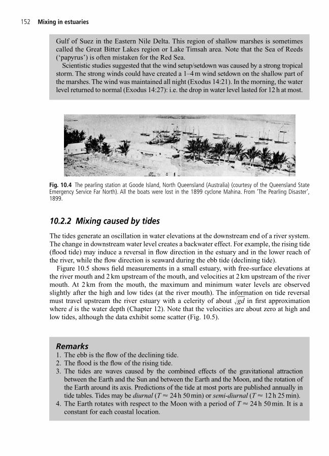
152 Mixing in estuaries

10.2.2 Mixing caused by tides

The tides generate an oscillation in water elevations at the downstream end of a river system.The change in downstream water level creates a backwater effect. For example, the rising tide(flood tide) may induce a reversal in flow direction in the estuary and in the lower reach ofthe river, while the flow direction is seaward during the ebb tide (declining tide).

Figure 10.5 shows field measurements in a small estuary, with free-surface elevations atthe river mouth and 2 km upstream of the mouth, and velocities at 2 km upstream of the rivermouth. At 2 km from the mouth, the maximum and minimum water levels are observedslightly after the high and low tides (at the river mouth). The information on tide reversalmust travel upstream the river estuary with a celerity of about ��gd in first approximationwhere d is the water depth (Chapter 12). Note that the velocities are about zero at high andlow tides, although the data exhibit some scatter (Fig. 10.5).

Gulf of Suez in the Eastern Nile Delta. This region of shallow marshes is sometimescalled the Great Bitter Lakes region or Lake Timsah area. Note that the Sea of Reeds(‘papyrus’) is often mistaken for the Red Sea.

Scientistic studies suggested that the wind setup/setdown was caused by a strong tropicalstorm. The strong winds could have created a 1–4 m wind setdown on the shallow part ofthe marshes. The wind was maintained all night (Exodus 14:21). In the morning, the waterlevel returned to normal (Exodus 14:27): i.e. the drop in water level lasted for 12 h at most.

Remarks1. The ebb is the flow of the declining tide.2. The flood is the flow of the rising tide.3. The tides are waves caused by the combined effects of the gravitational attraction

between the Earth and the Sun and between the Earth and the Moon, and the rotation ofthe Earth around its axis. Predictions of the tide at most ports are published annually intide tables. Tides may be diurnal (T � 24 h 50 min) or semi-diurnal (T � 12 h 25 min).

4. The Earth rotates with respect to the Moon with a period of T � 24 h 50 min. It is aconstant for each coastal location.

Fig. 10.4 The pearling station at Goode Island, North Queensland (Australia) (courtesy of the Queensland StateEmergency Service Far North). All the boats were lost in the 1899 cyclone Mahina. From ‘The Pearling Disaster’,1899.

10.2 Basic mechanisms 153

Shear effect in estuariesIn an estuary, the flow appears like a river but it goes back and forth with the tide. Friction ofthe tidal flow on the estuary boundaries generates turbulence and leads to turbulent mixing.The effects of flow oscillation on the longitudinal dispersion coefficient may be expressed as:

(10.4)

where K� is the longitudinal dispersion coefficient for a relatively long tidal period (T �� Tc),T is the tide period, Tc � W2/�t is the cross-sectional mixing time (or time scale for trans-verse mixing), W is the waterway width and �t is the rate of transverse mixing.

Shear flow dispersion has a maximum effect where the tide period T is similar to the timescale for transverse mixing Tc. For such conditions, the maximum dispersion coefficient equals:

(10.5)

where V is the mean tidal flow velocity. Equation (10.5) was developed assuming an uniform,long estuary with quasi-homogeneous density distribution. It provides an useful estimate ofthe dispersion in constant-density sections of an estuary, but it accounts for only the effect of(unsteady) shear flow.

The same analysis shows also much smaller dispersion coefficients in tidal flows than insimilar steady river flows (paragraph 10.4). For short tidal periods (T �� Tc), the concentra-tion distribution does not have time to respond to the changes in velocity profiles, and thelongitudinal dispersion coefficient tends towards 0 (Fischer et al. 1979).

K T T V T( ) .� c � 0 016

K K fTT

� �c

0

0.5

1

1.5

2

4:48 7:12 9:36 12:00 14:24 16:48�0.4

�0.2

0

0.2

0.4

Water depth AMTD 2 km Brisbane bar tidal gauge

Surface velocity AMTD 2 km Velocity 0.5 m below surface (AMTD 2 km)

Water depth (m)

Time (hh:mm)

Velocity (m/s)

Fig. 10.5 Experimental observations of water elevation and velocities in an estuary (after Chanson et al. 2003).Water depth, surface velocity and velocity measured 0.5 m beneath the free-surface in a meander of Eprapah Creekat 2.0 km upstream of the river mouth on 4 April 2003 – comparison with the tidal heights at the river mouth(Brisbane bar).

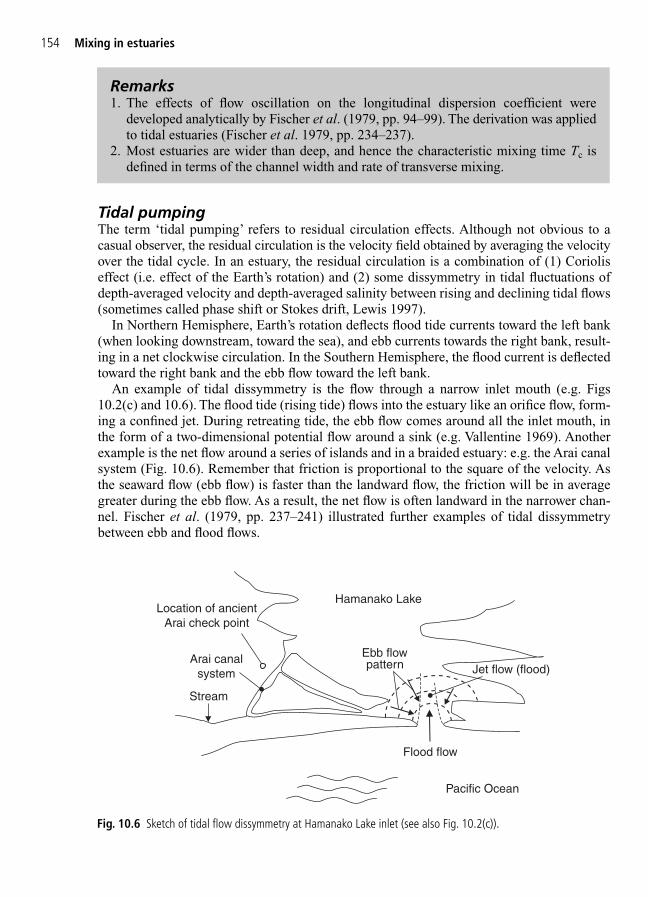
154 Mixing in estuaries

Tidal pumpingThe term ‘tidal pumping’ refers to residual circulation effects. Although not obvious to acasual observer, the residual circulation is the velocity field obtained by averaging the velocityover the tidal cycle. In an estuary, the residual circulation is a combination of (1) Corioliseffect (i.e. effect of the Earth’s rotation) and (2) some dissymmetry in tidal fluctuations ofdepth-averaged velocity and depth-averaged salinity between rising and declining tidal flows(sometimes called phase shift or Stokes drift, Lewis 1997).

In Northern Hemisphere, Earth’s rotation deflects flood tide currents toward the left bank(when looking downstream, toward the sea), and ebb currents towards the right bank, result-ing in a net clockwise circulation. In the Southern Hemisphere, the flood current is deflectedtoward the right bank and the ebb flow toward the left bank.

An example of tidal dissymmetry is the flow through a narrow inlet mouth (e.g. Figs10.2(c) and 10.6). The flood tide (rising tide) flows into the estuary like an orifice flow, form-ing a confined jet. During retreating tide, the ebb flow comes around all the inlet mouth, inthe form of a two-dimensional potential flow around a sink (e.g. Vallentine 1969). Anotherexample is the net flow around a series of islands and in a braided estuary: e.g. the Arai canalsystem (Fig. 10.6). Remember that friction is proportional to the square of the velocity. Asthe seaward flow (ebb flow) is faster than the landward flow, the friction will be in averagegreater during the ebb flow. As a result, the net flow is often landward in the narrower chan-nel. Fischer et al. (1979, pp. 237–241) illustrated further examples of tidal dissymmetrybetween ebb and flood flows.

Remarks1. The effects of flow oscillation on the longitudinal dispersion coefficient were

developed analytically by Fischer et al. (1979, pp. 94–99). The derivation was appliedto tidal estuaries (Fischer et al. 1979, pp. 234–237).

2. Most estuaries are wider than deep, and hence the characteristic mixing time Tc isdefined in terms of the channel width and rate of transverse mixing.

Pacific Ocean

Hamanako Lake

Arai canalsystem

Location of ancientArai check point

Stream

Flood flow

Jet flow (flood)Ebb flowpattern

Fig. 10.6 Sketch of tidal flow dissymmetry at Hamanako Lake inlet (see also Fig. 10.2(c)).

10.2 Basic mechanisms 155

Tidal trappingEstuaries, like rivers, are affected by ‘dead zones’. The role of such zones are enhanced bytidal action. The propagation of the tide in an estuary is a balance between the inertia of thewater mass, the pressure force due to the slope of the water surface and the retarding force ofbottom friction. As the tide changes, small dead zones have little momentum and the flowdirection will change as soon as the water level begins to drop. In contrast, the flow in the mainchannel has an initial momentum and the current will continue to flow against the opposingpressure gradient. This process will enhance longitudinal dispersion induced by the deadzones.

10.2.3 Mixing caused by the river

One, or more, rivers enter an estuary and deliver a freshwater discharge Q. The river is a sourceof buoyancy flux ��gQ, where �� is the density difference between the sea and the river. Inan estuary, a dimensionless measure of density stratification is the estuary Richardson numberdefined as:

where W is the channel width and Vt is the rms tidal velocity (Fischer et al. 1979). If Rit is verysmall, the estuary is well mixed (Fig. 10.1(c)), and density effects may be neglected. If Rit isvery large, the estuary is strongly stratified, and the flow motion is dominated by density cur-rents. For example, when a river discharges into an estuary connected to a tideless sea (e.g.Mediterranean Sea), the freshwater flows over the saltwater as an undiluted freshwater layer.Saltwater intrudes underneath the freshwater flow in the form of a wedge (Fig. 10.1(a)).

Rig Q

W Vt

t

���

� 3

Remarks1. The Coriolis force per unit mass (i.e. Coriolis acceleration) equals:

where V is the velocity of the fluid/object subjected to the Coriolis force, � is theangular velocity of the Earth (� � 2�/T ), T is the earth rotation period (T � 24 h)and is the latitude. If x is the coordinate in the flow direction, z is the vertical coordi-nate positive upwards and is positive in Northern Hemisphere, the Coriolis accelera-tion applies in the y-direction: i.e. to the left (when looking downstream) in the NorthernHemisphere and to the right in Southern Hemisphere.

2. Gustave Gaspard Coriolis (1792–1843) was a French mathematician and engineer ofthe ‘Corps des Ponts-et-Chaussées’ who first described the Coriolis force.

3. Located on the Enshu Coast along the Pacific Ocean, the Arai township is locatedabout half-distance between Tokyo and Osaka (Japan). It is on the right bank of theHamanako Lake esturary (Figs 10.2(c) and 10.6). During the Edo period, a maincheck point was located at Arai, controlling the traffic of weapons and movement ofpeople on the road to Edo (Tokyo).

�Coriolis sin2V�

156 Mixing in estuaries

Remarks1. Field observations suggest that the transition between well mixed to strongly stratified

estuary occurs for 0.08 � Rit � 0.8 (Fischer et al. 1979).2. Fischer et al. (1979) suggested a modified estuary Richardson number defined as:

Rit � (�� � g/�)Q/(W V*3), where V* is the rms shear velocity.

3. rms stands for root mean square.

Application: Stratification of the Pimpama Creek EstuaryPimpama Creek, Queensland is a small water system in Albert Shire, North of the GoldCoast. The catchment is very flat and made of acid soils. The creek is blocked by a weirat adopted middle thread distance (AMTD) measured upstream from the mouth 3.8 km(Fig. 7.2(c)). The structure is designed to prevent salt intrusion into the waterway. Gatesare only open during floods periods to relieve upstream flooding.

Detailed field measurements were conducted by the writer on 19 December 2002around 1:30 p.m. at AMTD 3.25 km, located downstream of the weir system. The timecorresponded to the mid ebb tide. The observations are given below.

The data showed a strong stratification of the estuary, although the system was mainlysaltwater (i.e. no brackish water) because of the weir gates were closed, preventing mixingbetween saltwater and freshwater. The top layer was warmer and saturated in oxygen.From 1.2 m below the free surface, the water was cooler and had low dissolved oxygencontents. On 19 December 2002, the tidal range was particularly important. At high tide,the river banks and mangroves were submerged. These waters were warmed up by thesun. During the ebb, the warmer, lighter waters flowed above the denser deep-channelwaters and the phenomenon induced the marked stratification.

Depth Temperature Dissolved oxygen Turbudity Conductivity pH Remarks (m) (!C) content (%) NTU mS/cm(1) (2) (3) (4) (5) (6) (7)

0.2 29.95 1.061 7 50.5 7.90.4 29.9 1.061 8 50.5 7.90.6 29.9 1.042 9 50.6 7.80.8 29.8 1.051 9 50.7 7.81 29.8 1.055 9 50.8 7.91.2 29.6 1.018 9 50.9 7.81.4 29.1 0.846 10 51.5 7.81.6 28.8 0.621 12 51.7 7.71.8 28.6 0.553 13 51.8 7.62 28.5 0.545 16 51.8 7.62.2 28.2 0.596 20 51.8 7.7 Just above

the bottom

Notes: Depth measured below the free surface; data collected during early ebb flow.

10.2.4 Discussion: mixing induced by tidal bores

When a river mouth has a flat, converging shape and when the tidal range exceeds 6–9 m,the river may experience a tidal bore (Fig. 10.7). A tidal bore is basically a series of waves

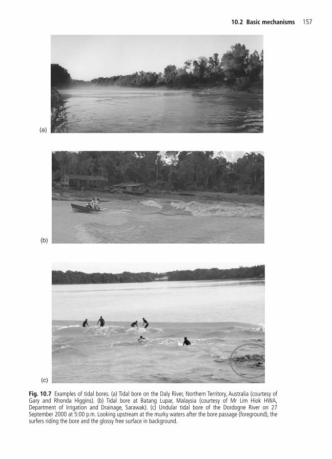
10.2 Basic mechanisms 157

(c)

Fig. 10.7 Examples of tidal bores. (a) Tidal bore on the Daly River, Northern Territory, Australia (courtesy ofGary and Rhonda Higgins). (b) Tidal bore at Batang Lupar, Malaysia (courtesy of Mr Lim Hiok HWA,Department of Irrigation and Drainage, Sarawak). (c) Undular tidal bore of the Dordogne River on 27September 2000 at 5:00 p.m. Looking upstream at the murky waters after the bore passage (foreground), thesurfers riding the bore and the glossy free surface in background.

(a)

(b)

158 Mixing in estuaries

propagating upstream as the tidal flow turns to rising. It is a positive surge (Chapter 12). Asthe surge progresses inland, the river flow is reversed behind it (e.g. Lynch 1982, Chanson 2001).

The best historically documented tidal bores are probably those of the Seine River (France)and Qiantang River (China). The mascaret of the Seine River was documented first duringthe 7th and 9th Centuries AD, and in writings from the 11th to 16th Centuries (Malandain 1988).It was locally known as ‘la Barre’. The Qiantang River bore, also called Hangzhou bore, wasearly mentioned during the 7th and 2nd Centuries BC. It was described in 8th Century writingsand later in a 16th Century Chinese novel.1 The bore was then known as ‘The Old Faithful’because it kept time better than clocks. A tidal bore on the Indus River might have wiped outthe fleet of Alexander the Great (Malandain 1988, Jones 2003). Another famous tidal bore isthe ‘pororoca’ of the Amazon River observed by V.Y. Pinzon and C.M. de La Condamine duringthe 16th and 18th Centuries respectively. The Hoogly (or Hooghly) bore on the Gange was doc-umented in 19th Century shipping reports. Smaller tidal bores occur on the Severn River nearGloucester, England, on the Garonne and Dordogne Rivers, France, at Turnagain Arm andKnik Arm, Cook Inlet (Alaska), in the Bay of Fundy (at Petitcodiac and Truro), on the Styxand Daly Rivers (Australia) and at Batang Lupar (Malaysia) (Fig. 10.7).

A tidal bore may affect shipping industries. For example, the mascaret of the Seine Riverhad had a sinister reputation. More than 220 ships were lost between 1789 and 1840 in theQuilleboeuf-Villequier section (Malandain 1988). The height of the mascaret bore couldreach up to 7.3 m and the bore front travelled at a celerity of about 2–10 m/s. Even in moderntimes, the Hoogly and Hangzhou bores are hazards for small ships and boats.

Tidal bores induce strong turbulent mixing in the estuary and river mouth. The effect maybe felt along considerable distances. With appropriate boundary conditions, a tidal bore maytravel far upstream: e.g. the tidal bore on the Pungue River (Mozambique) is still about 0.7 mhigh about 50 km upstream of the mouth and it may reach 80 km inland. Mixing and disper-sion in a tidal bore affected estuary are not comparable to well-mixed estuary processes.Instead the effects of the tidal bore must be accounted for and the bore may become the pre-dominant mixing process. The effect on sediment transport was studied at Petitcodiac andShubenacadie Rivers (Canada), in the Sée and Sélune Rivers (France), Ord River (Australia),Turnagain Arm inlet (Alaska) and on the Hangzhou bay (China) (e.g. Tessier and Terwindt1994, Bartsch-Winkler et al. 1985, Wolanski et al. 2001, Chen et al. 1990). The arrival of thebore front is associated with intense bed shear and scour. Behind sediment material isadvected upwards by large scale turbulent structures evidenced in Fig. 10.7(c). Sediment sus-pension behind the bore is sustained by strong long-lasting wave motion. At the Dee River(UK), Dr E. Jones observed more than 230 waves, also called whelps or éteules. Murphy’s(1983) photograph showed more than 30 well-formed undulations behind the Amazon poro-roca. At the Dordogne River (France), the writer observed an intense wave motion lastingmore than 20 min after the bore passage (Chanson 2001). Mixing and dispersion in a tidalbore affected estuary is not comparable to well-mixed estuary processes (e.g. Appendix C inChapter 7 and Appendix A, Section 10.6).

The impact of tidal bores on the ecology is acknowledged. In the Amazon River, piranhas eatmatter in suspension after the passage of the bore (Cousteau and Richards 1984). At TurnagainArm inlet, bald eagles and eagles were seen fishing behind the bore, while beluga whaleswere observed playing in the bore as it formed near the mouth of the arm (Bartsch-Winklerand Lynch 1988, Molchan-Douthit 1998). In the same estuary, a moose tried unsuccessfully

1 ‘Outlaws of the Marsh’, by Shi Nai’an and Luo Guanzhong. Foreign Languages Press, Beijing 1980. Written inthe 16th Century, the novel described historical events from the period AD 1100–1130.

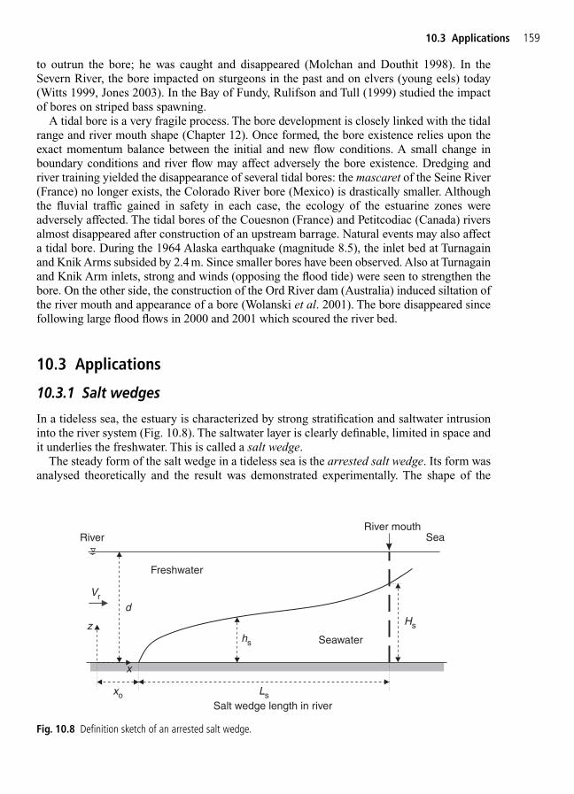
10.3 Applications 159

to outrun the bore; he was caught and disappeared (Molchan and Douthit 1998). In theSevern River, the bore impacted on sturgeons in the past and on elvers (young eels) today(Witts 1999, Jones 2003). In the Bay of Fundy, Rulifson and Tull (1999) studied the impactof bores on striped bass spawning.

A tidal bore is a very fragile process. The bore development is closely linked with the tidalrange and river mouth shape (Chapter 12). Once formed, the bore existence relies upon theexact momentum balance between the initial and new flow conditions. A small change inboundary conditions and river flow may affect adversely the bore existence. Dredging andriver training yielded the disappearance of several tidal bores: the mascaret of the Seine River(France) no longer exists, the Colorado River bore (Mexico) is drastically smaller. Althoughthe fluvial traffic gained in safety in each case, the ecology of the estuarine zones wereadversely affected. The tidal bores of the Couesnon (France) and Petitcodiac (Canada) riversalmost disappeared after construction of an upstream barrage. Natural events may also affecta tidal bore. During the 1964 Alaska earthquake (magnitude 8.5), the inlet bed at Turnagainand Knik Arms subsided by 2.4 m. Since smaller bores have been observed. Also at Turnagainand Knik Arm inlets, strong and winds (opposing the flood tide) were seen to strengthen thebore. On the other side, the construction of the Ord River dam (Australia) induced siltation ofthe river mouth and appearance of a bore (Wolanski et al. 2001). The bore disappeared sincefollowing large flood flows in 2000 and 2001 which scoured the river bed.

10.3 Applications

10.3.1 Salt wedges

In a tideless sea, the estuary is characterized by strong stratification and saltwater intrusioninto the river system (Fig. 10.8). The saltwater layer is clearly definable, limited in space andit underlies the freshwater. This is called a salt wedge.

The steady form of the salt wedge in a tideless sea is the arrested salt wedge. Its form wasanalysed theoretically and the result was demonstrated experimentally. The shape of the

River Sea

Vrd

hs

River mouth

z

LsSalt wedge length in river

Freshwater

Seawater

Hs

x

xo

Fig. 10.8 Definition sketch of an arrested salt wedge.

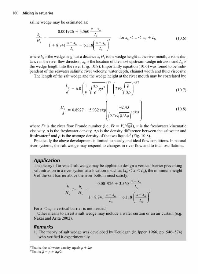
160 Mixing in estuaries

saline wedge may be estimated as:

(10.6)

where hs is the wedge height at a distance x, Hs is the wedge height at the river mouth, x is the dis-tance in the river flow direction, xo is the location of the most upstream wedge intrusion and Ls isthe wedge length into the river (Fig. 10.8). Importantly equation (10.6) was found to be inde-pendent of the seawater salinity, river velocity, water depth, channel width and fluid viscosity.

The length of the salt wedge and the wedge height at the river mouth may be correlated by:

(10.7)

(10.8)

where Fr is the river flow Froude number (i.e. Fr � Vr /√—gd ), � is the freshwater kinematic

viscosity, � is the freshwater density, �� is the density difference between the saltwater andfreshwater,2 and �– is the average density of the two liquids3 (Fig. 10.8).

Practically the above development is limited to steady and ideal flow conditions. In naturalriver systems, the salt wedge may respond to changes in river flow and to tidal oscillations.

Hd

Fr

s � �

�

0 8927 5 9322 43

20 2424

. . exp.

/.

−

( )

� �

Ld

gd Frs ��

�6 0

123

1 4 5 2

.�

�

�

�

�

−

hH

x xL

x xL

x xL

x x x Ls

s

o

s

o

s

o

s

o o S

1 8.741

for �

�

� �

0 001926 3 560

6 1182

. .

.

−

− −

ApplicationThe theory of arrested salt wedge may be applied to design a vertical barrier preventingsalt intrusion in a river system at a location x such as (xo � x � Ls), the minimum heighth of the salt barrier above the river bottom must satisfy:

For x � xo, a vertical barrier is not needed.Other means to arrest a salt wedge may include a water curtain or an air curtain (e.g.

Nakai and Arita 2002).

Remarks1. The theory of salt wedge was developed by Keulegan (in Ippen 1966, pp. 546–574)

who verified it experimentally.

hH

hH

x xL

x xL

x xL

s

s

s

o

s

o

s

o

s

1

� �

�

0 001926 3 560

8 741 6 1182

. .

. .

−

− −

2That is, the saltwater density equals � ��.3That is, –� � � ��/2.

10.3 Applications 161

10.3.2 Steady vertical circulation

Considering a well-mixed estuary, in a steady state case, the depth-averaged density increaseswith increasing distance x seaward. The slope of the mean water surface must counterbalancethe mean density gradient.

In the horizontal direction, the Navier–Stokes equation becomes:

(10.10)

where T is the eddy viscosity or momentum exchange coefficient in turbulent flow, P is thepressure, x is the horizontal coordinate and z is the vertical coordinate positive upward (Fig.10.9(a)). Note that equation (10.10) was developed assuming a negligible vertical velocitycomponent. For a steady flow and assuming that the advective term is small (i.e. V � ∂V/∂x � 0),the motion equation becomes:

(10.11)01 2

2 T� �

��

∂∂

∂∂

Px

V

z

∂∂

∂∂

∂∂

∂∂

Vx

VVx

Px

V

z T � �

1 2

2��

2. In equation (10.7), the term (1/ ) ����gd3����--� is analogous to a Reynolds number, calleddensimetric Reynolds number. The term 2Fr �

____�--/�� is some densimetric Froude

number, also called river flow parameter.3. For the height of the wedge at the river mouth, Keulegan obtained an analytical

expression:

(10.9)

Agreement between theory (equation (10.9)) and data was satisfactory when:

However, equation (10.8) provides a more accurate estimate for the range of flowconditions investigated in laboratory by Keulegan:

4. Equations (10.6) and (10.8) are best fits of a series of detailed experimental results.5. Garbis Hovannes Keulegan (1890–1989) was an Armenian mathematician who

worked as hydraulician for the US Bureau of Standards since its creation in 1932.

0 10 2 1 5. . "�

"Fr�

�

2Fr�

�� 1�

Hd

Frs � �11

22

2 3

2 3

/

�

��

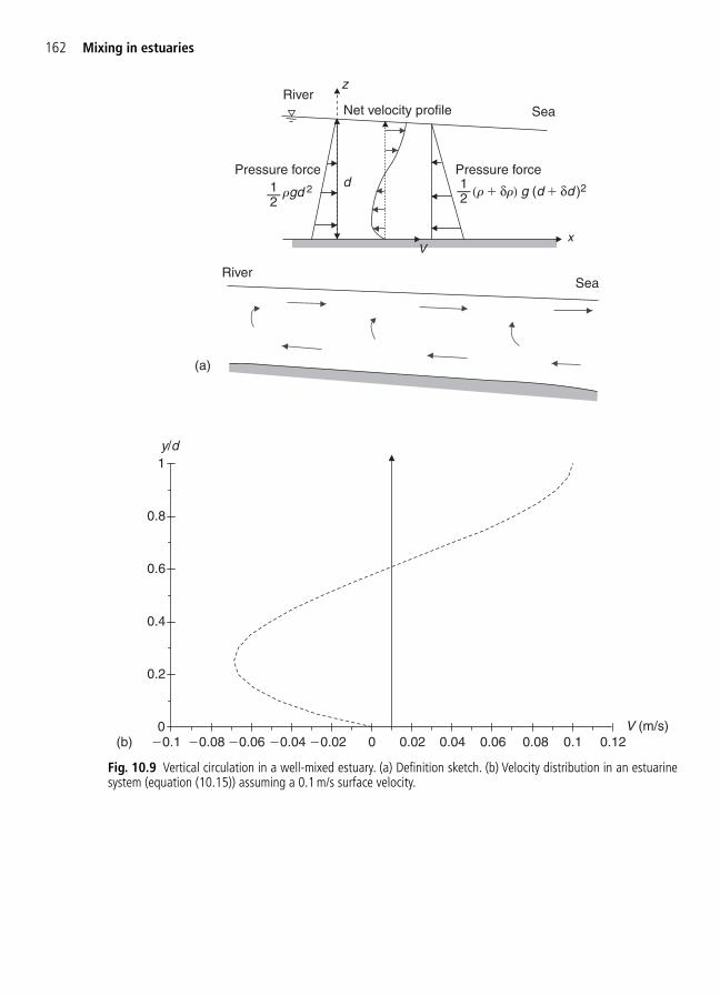
162 Mixing in estuaries

d

RiverSea

x

z

Pressure force Pressure force1—2

1—2rgd 2 (r δr) g (d δd )2

V

Net velocity profile

River

(a)

Sea

0

0.2

0.4

0.6

0.8

1

�0.1 �0.08 �0.06 �0.04 �0.02 0 0.02 0.04 0.06 0.08 0.1 0.12V (m/s)

y/d

(b)

Fig. 10.9 Vertical circulation in a well-mixed estuary. (a) Definition sketch. (b) Velocity distribution in an estuarinesystem (equation (10.15)) assuming a 0.1 m/s surface velocity.

10.3 Applications 163

At an elevation z, the pressure equals the weight of the water column above:

(10.12)

where � is the local fluid density and using the atmospheric pressure as a reference (i.e.P(z � d) � 0). Combining equations (10.11) and (10.12), it yields:

(10.13)

assuming a well-mixed estuary and where � is the depth-averaged density:

In first approximation, the integration of equation (10.13) yields:

(10.14)

where d is the water depth. Equation (10.14) expresses the relationship between the lon-gitudinal mean density gradient and the free-surface slope. It derives from momentum considerations and it yields:

The forces acting on a small vertical slice of the estuary are the pressure forces, the boundaryfriction and possibly the wind stress. At steady state, the solution of the motion equation givesthe velocity distribution:

(10.15)

where the momentum exchange coefficient �T is assumed constant with depth. Equation(10.15) predicts a steady circulation pattern, sketched in Fig. 10.9(a) and plotted in Fig.10.9(b) assuming a 0.1 m/s surface velocity. Note that a surface velocity V(z � d) of about0.1 m/s is enough to generate a recirculation flux much greater than the river flow.

Basically equation (10.15) characterizes a circulation pattern in the estuary, induced by thelongitudinal gradient in salinity and density. In turn, a weak salinity stratification produces anet mass transport across a vertical section which increases the stratification. Note that thecirculation flow is more important in deep waters.

V zgd

xzd

zd

zd

( ) ∂∂

−

T

� �3 2

488 15 6

��

�

∂∂

− ∂∂

dx x

��

∂∂

∂∂

dx

dx

� �38�

�

� � d�1

0dz

z

z d

=

=

∫

− ∂∂

∂∂

∂∂

gdx

gx

V

z T� �

�

��

2

20

P z g yy z

y d( ) d� �

=

=∫

Discussion: density-driven currents at the Strait of GibraltarThe Mediterranean Sea looses more water by evaporation that it receives freshwaterfrom rain and rivers. It is saltier than the Atlantic Ocean. The result is a strong Atlanticsurface water current (flowing westward) at the Strait of Gibraltar, while a deep, dense

164 Mixing in estuaries

10.4 Turbulent mixing and dispersion coefficients in estuaries

Estuaries are very complex systems and there are fundamental differences between salt-wedge estuaries, partially mixed estuaries and well-mixed estuaries (Fig. 10.1). Althoughestimate of mixing and dispersion coefficients should rely upon field tests, experimentalobservations are difficult and there is little systematic data on mixing and dispersion coeffi-cients in estuaries. Appendix A regroups a number of observations of mixing and dispersioncoefficients in estuarine zones. A small number of empirical correlations are shown in Table10.1. It is however extremely difficult to apply these.

Overall the measured values of mixing and dispersion coefficients are relatively smallcompared to mixing coefficients in rivers. By comparison, field observations in a

Mediterranean current, flows westward, near the bottom. The deep, westward currenttakes place about 120–150 m below the free surface.

The Strait of Gibraltar was called the Pillars of Hercules (Fretum Herculeum) by theAncients. Gibraltar is considered to have been one of the two Pillars of Hercules, theother being Mount Hacho, on the African Coast. The straight is 58 km long and it nar-rows to 13 km in width between Point Marroquí (Spain) and Point Cires (Morocco). Theaverage water depth is 365 m.

In the Antiquity, Phoenician sailors used heavy, ballasted sea-anchors (sank in the bot-tom current) to pull their boats into the Atlantic Ocean. Jacques Cousteau repeated theexperiment with the Calypso in the 1980s.4 During World War II, German submarinesused the surface water current and rising tide to pass silently the Strait of Gibraltar intothe Mediterranean Sea.

Notes1. The Navier–Stokes equation was first derived by L. Navier in 1822 and S.D. Poisson

in 1829 by an entirely different method. They were later derived by Barré de Saint-Venant in 1843 and G.G. Stokes in 1845.

2. Louis Navier (1785–1835) was a French engineer who primarily designed bridge butalso extended Euler’s equations of motion. Siméon Denis Poisson (1781–1840) was aFrench mathematician and scientist. He developed the theory of elasticity, a theory ofelectricity and a theory of magnetism. Adhémar Jean Claude Barré de Saint-Venant(1797–1886), French engineer, developed the equations of motion of a fluid particlein terms of the shear and normal forces exerted on it. George Gabriel Stokes(1819–1903), British mathematician and physicist, is known for his research inhydrodynamics and a study of elasticity.

3. Equations (10.14) and (10.15) were developed for an idealized, two-dimensional,horizontal estuary, assuming a steady state, no wind shear stress and negligible fresh-water inflow compared to the recirculation flow (Lewis 1997, p. 66).

4. The integration was performed assuming a constant momentum exchange coefficientwith depth (i.e. �T(z) � constant).

4Cousteau, J.Y., and Paccalet, Y. (1987). Méditerranée: la mer blessée. Flammarion, 192 pp.

10.5 Applications 165

meandering reach of the Missouri River yielded: �t � 0.12 m2/s and K � 1500 m2/s forV � 1.55 m/s, d � 2.7 m, W � 200 m, V* � 0.074 m (Fischer et al. 1979, pp. 110 and 126).

10.5 Applications

10.5.1 Application no. 1: Ino-hana Lake, Hama-matsu (Japan)

Ino-hana Lake is a shallow water lake near Hama-matsu (Japan) (Fig. 10.10). This saltwaterbody is connected to Hamanako Lake (Fig. 10.2(c)) and it is alimented in freshwater by several

Fig. 10.10 Ino-Hana Lake on 1 April 1999, shortly after a very strong wind storm during which a boat sunk and anearby road was overtopped by wind waves – looking North.

Table 10.1 Empirical estimates of mixing coefficients in estuarine zones

Coefficient Correlation Remarks (1) (2) (3)

Vertical mixing coefficient Well-mixed river flow

Well-mixed river flow. At mid-depth, where�V � amplitude of depth-averaged current.After Bowden

Longitudinal dispersion coefficient Well-mixed system. Vs � amplitude ofsurface tidal current. Assuming bed velocityis zero. After Bowden

��v

*

dV0 067.

KV d

s

v�

�

2 2

240

��v

d V�0 0025.

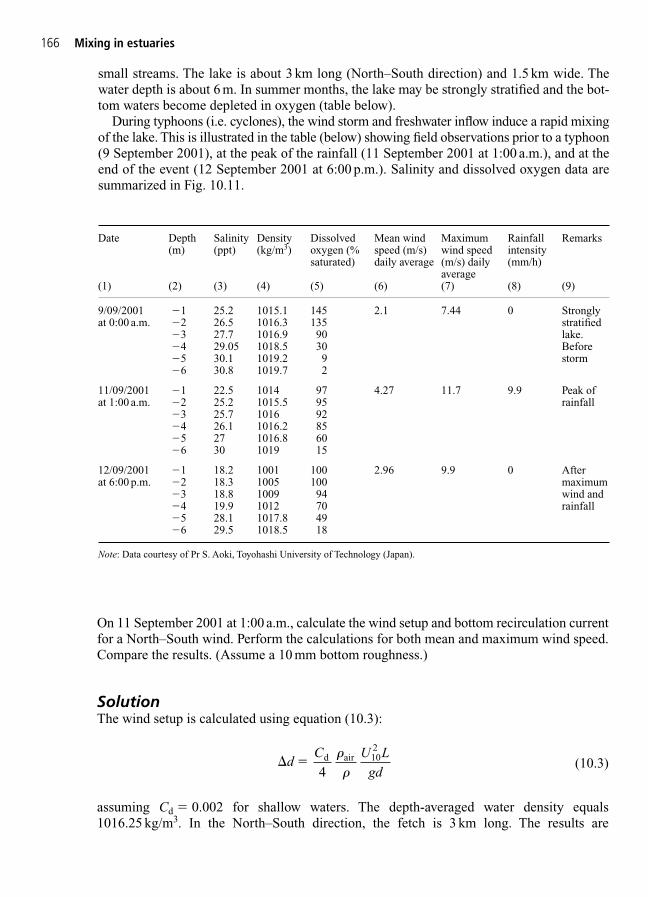
166 Mixing in estuaries

Date Depth Salinity Density Dissolved Mean wind Maximum Rainfall Remarks (m) (ppt) (kg/m3) oxygen (% speed (m/s) wind speed intensity

saturated) daily average (m/s) daily (mm/h) average

(1) (2) (3) (4) (5) (6) (7) (8) (9)

9/09/2001 �1 25.2 1015.1 145 2.1 7.44 0 Stronglyat 0:00 a.m. �2 26.5 1016.3 135 stratified

�3 27.7 1016.9 90 lake.�4 29.05 1018.5 30 Before�5 30.1 1019.2 9 storm�6 30.8 1019.7 2

11/09/2001 �1 22.5 1014 97 4.27 11.7 9.9 Peak of at 1:00 a.m. �2 25.2 1015.5 95 rainfall

�3 25.7 1016 92�4 26.1 1016.2 85�5 27 1016.8 60�6 30 1019 15

12/09/2001 �1 18.2 1001 100 2.96 9.9 0 After at 6:00 p.m. �2 18.3 1005 100 maximum

�3 18.8 1009 94 wind and �4 19.9 1012 70 rainfall�5 28.1 1017.8 49�6 29.5 1018.5 18

Note: Data courtesy of Pr S. Aoki, Toyohashi University of Technology (Japan).

small streams. The lake is about 3 km long (North–South direction) and 1.5 km wide. Thewater depth is about 6 m. In summer months, the lake may be strongly stratified and the bot-tom waters become depleted in oxygen (table below).

During typhoons (i.e. cyclones), the wind storm and freshwater inflow induce a rapid mixingof the lake. This is illustrated in the table (below) showing field observations prior to a typhoon(9 September 2001), at the peak of the rainfall (11 September 2001 at 1:00 a.m.), and at theend of the event (12 September 2001 at 6:00 p.m.). Salinity and dissolved oxygen data aresummarized in Fig. 10.11.

On 11 September 2001 at 1:00 a.m., calculate the wind setup and bottom recirculation currentfor a North–South wind. Perform the calculations for both mean and maximum wind speed.Compare the results. (Assume a 10 mm bottom roughness.)

SolutionThe wind setup is calculated using equation (10.3):

(10.3)

assuming Cd � 0.002 for shallow waters. The depth-averaged water density equals1016.25 kg/m3. In the North–South direction, the fetch is 3 km long. The results are

�dC U L

gd d air�

4102�

�

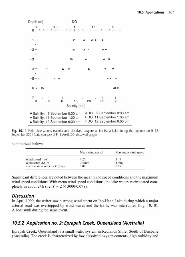
10.5 Applications 167

summarized below:

0

0 5 10 15 20 25 30

0 0.5

Salinity, 9 September 0:00 amSalinity, 11 September 1:00 amSalinity, 12 September 6:00 pm

DO, 9 September 0:00 amDO, 11 September 1:00 amDO, 12 September 6:00 pm

Salinity (ppt)

DODepth (m)

1 1.5 2

�1

�2

�3

�4

�5

�6

�7

Fig. 10.11 Field observations (salinity and dissolved oxygen) at Ino-Hana Lake during the typhoon on 9–12September 2001 (data courtesy of Pr S. Aoki). DO: dissolved oxygen.

Mean wind speed Maximum wind speed

Wind speed (m/s) 4.27 11.7Wind setup �d (m) 0.5 mm 4 mmRecirculation velocity V (m/s) 0.07 0.18

Significant differences are noted between the mean wind speed conditions and the maximumwind speed conditions. With mean wind speed conditions, the lake waters recirculated com-pletely in about 24 h (i.e. T � 2 � 3000/0.07 s).

DiscussionIn April 1999, the writer saw a strong wind storm on Ino-Hana Lake during which a majorarterial road was overtopped by wind waves and the traffic was interrupted (Fig. 10.10).A boat sunk during the same event.

10.5.2 Application no. 2: Eprapah Creek, Queensland (Australia)

Eprapah Creek, Queensland is a small water system in Redlands Shire, South of Brisbane(Australia). The creek is characterized by low dissolved oxygen contents, high turbidity and

168 Mixing in estuaries

nutrient concentrations. Field measurements were conducted in Eprapah Creek on 7 February1996 in the estuarine zone (Fig. 10.12). The data are summarized below.

Fig. 10.12 Eprapah Creek, Redlands, Queensland on 24 June 1999 (courtesy of the Waterways Scientific Services,Queensland Environment Protection Agency). Note exotic waterweeds. The creek is characterized by low dissolvedoxygen contents, high turbidity and nutrient concentrations.

Notes1. Turbidity refers to cloudiness caused by very small particles of silt, clay and other

substances suspended in water.2. AMTD is the distance upstream measured from the river mouth, following the

riverbed. AMTD � 0 is the river mouth.

Date AMTD (km) depth (m) Salinity (ppt) (g/L)(1) (2) (3) (4)

07-02-96 0 0.2 34.430 1.5 34.42 0.2 28.732 2 33.462 3 33.632.4 0.2 27.312.4 2 29.092.7 0.2 21.862.7 2 26.962.7 3 26.99

Note: Depth: measured below the free surface.Source: Data courtesy of Queensland Environment Protection Agency.

(a) Calculate the slope of the mean water surface to counterbalance the mean density gradi-ent between AMTD � 2000 and 2700 m. (b) Predict the velocity profile at the river mouth

10.5 Applications 169

0

1

2

3

4

�0.03 �0.02 �0.01 0 0.01 0.02 0.03Velocity (m/s)

Depth (m) Eprapah Creek

Fig. 10.13 Estimated velocity distribution at AMTD 2.4 km (Eprapah Creek).

and at AMTD � 2400 m. Neglect the bed slope. Assume an average water depth of 4 mand �T � 0.003 m2/s.

SolutionFirst the data must be analysed to obtain the depth-averaged density. It yields:

The water density is almost constant between AMTD 2 km and the river mouth (AMTD �0). Between AMTD 2 and 2.7 km, the average density gradient is: ∂�/∂x � 7.0 � 10�3kg/m4.In turn this implies a water level slope ∂d/∂x � �1.0 � 10�5 to compensate for the mean den-sity gradient. Assuming a reasonably well-mixed system, the steady vertical circulationyields a surface velocity of 0.03 m/s. The velocity profile is plotted in Fig. 10.13.

DiscussionChanson et al. (2003) conducted a similar analysis at Epapah Creek based upon some fieldwork in April 2003. Their results implied also some residual circulation leading to a renewalof the estuarine waters in about 1 week.

10.5.3 Application no. 3: Strait of Gibraltar

The Strait of Gibraltar is 13 km wide at the narrowest point and the average water depth is365 m. The Mediterranean saline waters have a salinity of about 38 ppt, corresponding to a

Date AMTD (km) Depth-averaged density (kg/m3)(1) (2) (3)

07-02-96 0 1023.62 10222.4 1019.32.7 1017

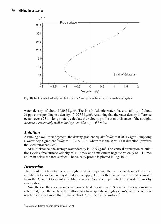
170 Mixing in estuaries

water density of about 1030.5 kg/m3. The North Atlantic waters have a salinity of about36 ppt, corresponding to a density of 1027.5 kg/m3. Assuming that the water density differenceoccurs over a 23 km long stretch, calculate the velocity profile at mid-distance of the straight.Assume a reasonably well-mixed system. Use T � 0.8 m2/s.

SolutionAssuming a well-mixed system, the density gradient equals: ∂�/∂x � 0.00013 kg/m4, implyinga water depth gradient ∂d/∂x � �1.7 � 10�5, where x is the West–East direction (towardsthe Mediterranean Sea).

At mid-distance, the average water density is 1029 kg/m3. The vertical circulation calcula-tions yield a free-surface velocity of 1.6 m/s, and a maximum negative velocity of �1.1 m/sat 275 m below the free surface. The velocity profile is plotted in Fig. 10.14.

DiscussionThe Strait of Gibraltar is a strongly stratified system. Hence the analysis of vertical circulation for well-mixed system does not apply. Further there is net flux of fresh seawaterfrom the Atlantic Ocean into the Mediterranean Sea to compensate for the water losses byevaporation.

Nonetheless, the above results are close to field measurement. Scientific observations indi-cated that, near the surface the inflow may have speeds as high as 2 m/s, and the outflowreaches speeds of more than 1 m/s at about 275 m below the surface.5

0

50

100

150

200

250

300

350

�2 �1.5 �1 �0.5 0.5 1.5

Velocity (m/s)

z (m)

Strait of Gibraltar

Free surface

1 20

Fig. 10.14 Estimated velocity distribution in the Strait of Gibraltar assuming a well-mixed system.

5Reference: Encyclopedia Britannica (1997).

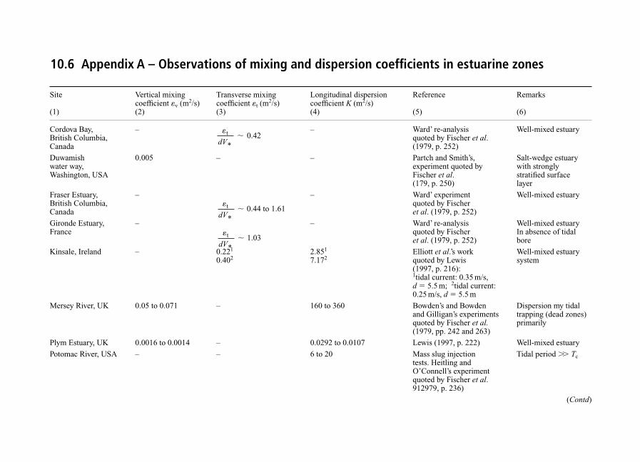
Site Vertical mixing Transverse mixing Longitudinal dispersion Reference Remarkscoefficient �v (m2/s) coefficient �t (m2/s) coefficient K (m2/s)

(1) (2) (3) (4) (5) (6)

Cordova Bay, – – Ward’ re-analysis Well-mixed estuaryBritish Columbia, quoted by Fischer et al.Canada (1979, p. 252)

Duwamish 0.005 – – Partch and Smith’s, Salt-wedge estuarywater way, experiment quoted by with stronglyWashington, USA Fischer et al. stratified surface

(179, p. 250) layer

Fraser Estuary, – – Ward’ experiment Well-mixed estuaryBritish Columbia, quoted by Fischer Canada et al. (1979, p. 252)

Gironde Estuary, – – Ward’ re-analysis Well-mixed estuaryFrance quoted by Fischer In absence of tidal

et al. (1979, p. 252) bore

Kinsale, Ireland – 0.221 2.851 Elliott et al.’s work Well-mixed estuary0.402 7.172 quoted by Lewis system

(1997, p. 216): 1tidal current: 0.35 m/s, d � 5.5 m; 2tidal current: 0.25 m/s, d � 5.5 m

Mersey River, UK 0.05 to 0.071 – 160 to 360 Bowden’s and Bowden Dispersion my tidaland Gilligan’s experiments trapping (dead zones)quoted by Fischer et al. primarily(1979, pp. 242 and 263)

Plym Estuary, UK 0.0016 to 0.0014 – 0.0292 to 0.0107 Lewis (1997, p. 222) Well-mixed estuary

Potomac River, USA – – 6 to 20 Mass slug injection Tidal period �� Tctests. Heitling and O’Connell’s experiment quoted by Fischer et al.912979, p. 236)

(Contd)

�t

*

dV� 0 42.

�t

* 0.44 to 1.61

dV�

10.6 Appendix A – Observations of mixing and dispersion coefficients in estuarine zones

�t

* 1.03

dV�

Site Vertical mixing Transverse mixing Longitudinal dispersion Reference Remarkscoefficient �v (m2/s) coefficient �t (m2/s) coefficient K (m2/s)

(1) (2) (3) (4) (5) (6)

San Francisco – 2002 1Ward’ re-analysis Well-mixed estuaryBay, USA quoted by Fischer et al.

(1979, p. 252) 2 Glenne and Selleck’s experiment quoted by Fischer et al.(1979, p. 263)

Severn River, UK 0.0024 to 0.0111 0.021 to 0.0141 54 to 5402 1Elliott et al.’s work Well-mixed estuary.quoted by Lewis River affected by(1997, p. 296) a tidal bore2Bowden’s experiment quoted by Fischer et al. (1969, p. 263)

Strangford Lough, – 0.161 1.191 Elliott et al.’s work quoted Well-mixed systemIreland 0.192 2.132 by Lewis (1997, p. 216):

1tidal current: 0.5 m/s,d � 10 m; 2tidal current:0.12 m/s, d � 6.5 m

Tees Estuary, UK 0.001 to 0.0016 – 0.0547 to 0.0580 Lewis (1997, p. 222) Well-mixed estuary

Thames River, UK – – 53 to 841 1Bowden’s experiments 3382 quoted by Fischer et al.

(1969, p. 263)2For high river flow

�t 1

* 1.0

dV�

10.7 Exercises 173

10.6.1 Field observations of mixing in tidal bores

Field measurements in tidal bores are scarce. Kjerfve and Ferreira (1993) and Wolanski et al.(2001) reported observations of sediment mixing immediately behind bores in the RioMearim (Brazil) and Ord River (Australia) respectively. Bartsch-Winkler and Lynch (1988)dropped bags of dye in the Turnagain Arm bore. Rulifson and Tull (1999) discussed the lon-gitudinal dispersion of fish eggs in tidal bore affected rivers in the Bay of Fundy (Canada).Kjerfve and Ferreira (1993) presented quantitative measurements of salinity and temperaturechanges behind a bore. Their data highlighted a sharp jump in water properties about 18 minafter the bore passage at two locations, while a rapid change in salinity was observed 42 minafter the bore passage at a more upstream location.

Two fascinating experiments were conducted by M. Partiot in the Seine River mouth (inBazin 1865b, pp. 640–641). The experiments highlighted different flow patterns next to thesurface and at deeper depths. On 13 September 1855, in front of the Chapel Barre-y-Va(downstream of Caudebec-en-Caux), two floats were introduced in the river flow (a) at the sur-face and (b) next to the bottom (3.3 m beneath the surface). When the undular bore arrived, thesurface float (a) continued to flow downstream for 130 s after the bore passage and flowedupstream afterwards, while the bottom float (b) flowed downstream only 90 s after the borepassage. On 25 September 1855, in front of Vallon de Caudebecquet, three floats were intro-duced (a) at the surface, (b) 1.5 m beneath the surface and (c) next to the bottom, all in the mid-dle of the river. At the undular surge arrival, the float (a) started to run upstream 145 s after thebore passage, while the floats (b) and (c) flowed upstream 60 s after the bore passing.

10.7 Exercises

1. The estuary of the Flora River is 240 m long and 17 m wide. At high tide, the averagewater depth is 3.5 m. Calculate the wind setup for a 25 m/s wind blowing along the mainaxis of the estuary. Estimate the cross-sectional mixing time and compare the result withthe tidal period. Estimate the bottom current assuming a bottom roughness ks � 5 mm.The tidal regime is semi-diurnal. The transverse mixing coefficient is assumed to be0.007 m2/s.

2. A lagoon on the North Coast of Papua New Guinea extends along 15 km of the shorelineand is about 250 m wide in average. The mean water depth is 0.9 m. Calculate the windsetup for a 22 m/s wind blowing parallel to the shoreline and perpendicular to the coast.Estimate the resonance frequencies of the lagoon. The resonance frequency of a waterbody is the ‘sloshing’ frequency of the seiche.

3. The estuary of the Loup River, Nice (France) is affected by a salt-wedge system. The riverwidth is about 25 m. For a 4.8 m3/s flow rate, the water depth is about 1.5 m. Calculate thelength of the salt wedge, the height of the wedge at the river mouth, and the saline wedgeheight at 90 m upstream of the river mouth. Use Keulegan’s theory. Assume Var River den-sity of 1012 kg/m3 (because of suspended sediments).

4. A river flow into a tideless sea. The river flow velocity is 0.15 m/s and the mean water depthis 1.35 m. A salt barrier is to be built 50 m upstream of the river mouth to prevent salt intru-sion into the river system and on the water table. Calculate the minimum salt barrier height.

5. A reasonably well-mixed estuary is about 1200 m long. The depth-averaged density variesbetween 1005 and 1022 kg/m3 over that distance, and the average water depth 2.4 m.Calculate the required longitudinal free-surface gradient. Plot the velocity profile in the

0

0.5

1

1.5

2

2.5

3

3.5

4

0.4 0.5 0.6 0.7 0.8 0.9

10 20 30 40 50

DOC at AMTD 2 kmDOC at AMTD 3.2 km

Conductivity AMTD 2 kmConductivity AMTD 3.2 km

Cabbage Tree Creek, AMTD 2 and 3.2 km,12 February 2003

DOC

Conductivity (mS/cm)

Fig. 10.16 Vertical distribution of conductivity and dissolved oxygen content at Cabbage Tree Creek on 12 February2003. DOC: dissolved oxygen content.

174 Mixing in estuaries

estuary (assuming �T � 0.001 m2/s). Estimate the free-surface velocity and the maximumnegative velocity.

6. The Knysna Bay Estuary in the Southern Cape (South Africa) is 230 m wide with an aver-age channel depth of approximately 10 m. The longitudinal gradient in average density

Fig. 10.15 Cabbage Tree Creek, Brisbane, Queensland on 12 February 2003 near AMTD 2.0 km – looking upstream.

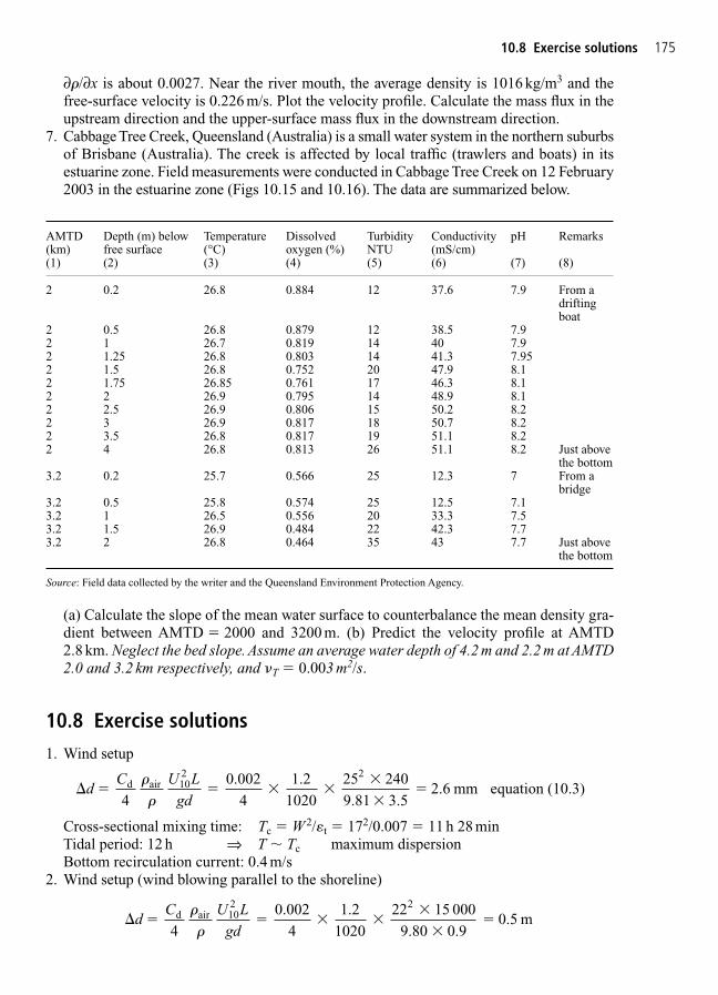
10.8 Exercise solutions 175

(a) Calculate the slope of the mean water surface to counterbalance the mean density gra-dient between AMTD � 2000 and 3200 m. (b) Predict the velocity profile at AMTD2.8 km. Neglect the bed slope. Assume an average water depth of 4.2 m and 2.2 m at AMTD2.0 and 3.2 km respectively, and T � 0.003 m2/s.

10.8 Exercise solutions

1. Wind setup

Cross-sectional mixing time: Tc � W2/�t � 172/0.007 � 11 h 28 minTidal period: 12 h ⇒ T � Tc maximum dispersionBottom recirculation current: 0.4 m/s

2. Wind setup (wind blowing parallel to the shoreline)

� � � � ��

��d

C U Lgd

4

0.002

4

1.21020

22 15 000

0.9 0.5 md air 10

2 2�

� 9 80.

� � � � ��

��d

C U Lgd

4

0.002

4

1.21020

25 240

3.5 2.6 mm equation (10.3)d air 10

2 2�

� 9 81.

AMTD Depth (m) below Temperature Dissolved Turbidity Conductivity pH Remarks (km) free surface (°C) oxygen (%) NTU (mS/cm)(1) (2) (3) (4) (5) (6) (7) (8)

2 0.2 26.8 0.884 12 37.6 7.9 From adriftingboat

2 0.5 26.8 0.879 12 38.5 7.92 1 26.7 0.819 14 40 7.92 1.25 26.8 0.803 14 41.3 7.952 1.5 26.8 0.752 20 47.9 8.12 1.75 26.85 0.761 17 46.3 8.12 2 26.9 0.795 14 48.9 8.12 2.5 26.9 0.806 15 50.2 8.22 3 26.9 0.817 18 50.7 8.22 3.5 26.8 0.817 19 51.1 8.22 4 26.8 0.813 26 51.1 8.2 Just above

the bottom3.2 0.2 25.7 0.566 25 12.3 7 From a

bridge3.2 0.5 25.8 0.574 25 12.5 7.13.2 1 26.5 0.556 20 33.3 7.53.2 1.5 26.9 0.484 22 42.3 7.73.2 2 26.8 0.464 35 43 7.7 Just above

the bottom

Source: Field data collected by the writer and the Queensland Environment Protection Agency.

∂�/∂x is about 0.0027. Near the river mouth, the average density is 1016 kg/m3 and thefree-surface velocity is 0.226 m/s. Plot the velocity profile. Calculate the mass flux in theupstream direction and the upper-surface mass flux in the downstream direction.

7. Cabbage Tree Creek, Queensland (Australia) is a small water system in the northern suburbsof Brisbane (Australia). The creek is affected by local traffic (trawlers and boats) in itsestuarine zone. Field measurements were conducted in Cabbage Tree Creek on 12 February2003 in the estuarine zone (Figs 10.15 and 10.16). The data are summarized below.

176 Mixing in estuaries

Wind setup (wind blowing normal to the shoreline)

The resonance period of water body is approximately 2L /�gd Hence:resonance frequency along major axis � 0.0001 Hz (T � 2 h 48 min) andresonance frequency along minor axis � 0.006 Hz (T � 168 s)

3. Salt wedge (Loup River)Hs � 0.76 m, Ls � 853 m, hs � 0.62 m (90 m upstream of the river mouth).

4. Salt barrierSalt wedge: Hs � 0.74 m, Ls � 1260 m.Salt barrier: minimum height, h � 0.68 m (50 m upstream of the river mouth).

5. ∂d/∂x � �1.3 � 105

Free-surface velocity � 0.04m/s, maximum negative velocity � �0.027 m/s. (atz/d � 0.3)

6. The momentum exchange coefficient must be first calculated: T � 0.024 m2/s.At equilibrium, the mass flux in the downstream direction equals the mass flux in theupstream direction (i.e. 0.58 m2/s).

� � � � ��

��d

C U Lgd

4

0.002

4

1.21020

22 250

0.9 8 mmd air 10

2 2�

� 9 80.

Part 2 Revision exercises

1. The Waikato River, near Hamilton, New Zealand has the following channel characteris-tics: Q � 150 m3/s, d � 2.5 m, width: 85 m, V � 0.7 m/s, V* � 0.057 m/s.A first dye test will be conducted by injecting continuously a tracer (Lissamine Red 4B) atthe side (125 g/s).(a) Calculate the distance from the injection point where the tracer concentration reach

10 mg/m3 on the opposite bank. Assume an infinitely wide rectangular channel forsimplicity and neglect vertical mixing (for question (a) only).

In a second dye test, a mass slug of dye (2.5 kg) is suddenly released on the centreline.(b) Predict the dispersion coefficient and the length of the initial zone.A measurement station is located 15 km downstream of the injection point (second test).(c) Calculate the maximum tracer concentration at that station and the arrival time.(d) The detection limit of Lissamine Red 4B dye is 0.1 mg/m3. Calculate the length of

time during Lissamine dye will be detectable at the measurement station.(e) At the time when the tracer concentration is maximum at the station, calculate the

cloud length with concentrations exceeding 0.5 mg/m3.

* * *

2. A chemical is accidentally released in a natural stream between 1:30 a.m. and 2:30 a.m. (atnight) at a rate of 7 kg/h (top hat inflow). Calculate the period during which concentrationexceed 1.5 mg/m3, as well as the maximum concentration, at a site located 12 km downstreamof the source. The river characteristics are: Q � 5 m3/s, width: 25 m, bed slope: 0.00025,gravel bed: ks � 25 mm. Approximate the top hat discharge by four mass slugs of 1.75 kgreleased at 1:37 a.m.,1:52 a.m., 2:07 a.m. and 2:22 a.m.

* * *

3. Dye profiles were measured at the Manawatu River, below Palmerston North (NewZealand). The table below shows cross-sectional averaged dye concentrations at two meas-urement sites located respectively 5.0 and 6.4 km downstream of the injection point. (Pre-liminary calculations suggested that the site locations were downstream of the initial zone.)(a) Using the frozen cloud approximation, estimate the flow velocity and longitudinal dis-

persion coefficient between the two measurement sites.(b) Using a ADZ ‘dead zone’ model, predict the dye concentration versus time at the sec-

ond measurement location, and compare it with the ‘frozen cloud’ dispersion model.Assume a conservative tracer.

178 Revision exercises

Location Time (h) Cm (mg/m3) Location Time (h) Cm (mg/m3)(1) (2) (3) (4) (5) (6)

Site 1 2.106 0.833 Site 2 2.85 1.96Site 1 2.19 9.58 Site 2 2.93 5.96Site 1 2.27 11.8 Site 2 3 10.6Site 1 2.37 14.9 Site 2 3.12 14Site 1 2.445 21.9 Site 2 3.18 21.15Site 1 2.52 26.9 Site 2 3.22 23.92Site 1 2.62 29.2 Site 2 3.24 24.33Site 1 2.675 35 Site 2 3.295 27.25Site 1 2.78 36.4 Site 2 3.345 25.8Site 1 2.85 36.3 Site 2 3.379 32.7Site 1 2.93 36.2 Site 2 3.404 33.3Site 1 3 35.8 Site 2 3.48 33.5Site 1 3.12 31.9 Site 2 3.53 34.29Site 1 3.18 29.6 Site 2 3.596 35.1Site 1 3.27 29.2 Site 2 3.638 34.7Site 1 3.345 25.3 Site 2 3.722 34.5Site 1 3.43 23.46 Site 2 3.76 33.7Site 1 3.51 21.7 Site 2 3.83 32.8Site 1 3.59 17.9 Site 2 3.915 29.4Site 1 3.68 16.4 Site 2 3.965 29.8Site 1 3.755 14.17 Site 2 4.14 24.3Site 1 3.84 12.8 Site 2 4.2 23.5Site 1 3.93 10.8 Site 2 4.26 21.9Site 1 4 10.17 Site 2 4.33 21.6Site 1 4.1 8.92 Site 2 4.39 19.9Site 1 4.2 8.08 Site 2 4.5 16Site 1 4.31 7 Site 2 4.97 9.5Site 1 4.39 6.04 Site 2 5.133 6.5Site 1 4.51 5 Site 2 5.44 4.5Site 1 4.71 3.92 Site 2 5.52 3.29Site 1 4.79 3.25 Site 2 5.84 3.25Site 1 4.89 2.83 Site 2 6 2.17Site 1 5 2.3 Site 2 6.25 1.58Site 1 5.1 2.17 Site 2 6.5 1.17Site 1 5.2 2 Site 2 6.75 0.96Site 1 5.3 1.75 Site 2 7 0.83Site 1 5.4 1.67Site 1 5.5 1.38Site 1 5.75 1.17Site 1 6 0.83Site 1 6.25 0.625Site 1 6.5 0.375Site 1 6.75 0.33Site 1 7 0.25

Note: Data from Rutherford (1994, pp. 271–273).

Conditions Q Average Average Bed roughness Water Dissolved BOD5(m3/s) width bed slope height temperature oxygen (kg/m3)

(m) (mm) (°C) content (%)

1 1 2 0.00012 10 20 752 1.5 2 0.00012 10 20 753 12 3 0.00012 25 20 85

4. Investigations are undertaken for a scheme to increase waste water effluent release inHilliard Creek. To assist the environmental impact study, calculations are conducted for thefollowing flow conditions:

* * *

The water treatment plant is to discharge some effluent into the creek at a rate of 0.45 m3/swith a BOD5 is 270 g/m3. Calculate the minimum DOC downstream of the injection pointand its location. Estimate the BOD5 for a sample taken at that location. Assume the efflu-ent to be at the same temperature as the river. Assume further that the wastewater spreadsalmost instantaneously across the entire section.

* * *5. A chemical is accidentally released in a natural stream between 1:00 a.m. and 3:00 a.m. at

a rate of 25 kg/h for the first 45 min and later 10 kg/h for the next 75 min. Calculate theperiod during which concentration exceeds 0.05 mg/m3 as well as the maximum concen-tration, at a site located 20 km downstream of the source. Plot the chemical concentrationversus time on the same graph. The river characteristics are: Q � 3.3 m3/s, width: 15 m,bed slope: 0.000 28, small gravel bed: ks � 25 mm. Approximate the chemical release by asuccession of mass slugs and apply the method of superposition.

Assignment solutions

1. (a) �t � 0.085 m2/s equation (7.6)

equation (7.7)

by applying the principle of superposition and the method of images. (In the virtualstream, the injection rate is 2 � 125 g/s.) It yields: x � 4065 m.

(b) K � 273 m2/sInitial region: L � 5900 m

(c) Cmax � 1.37 � 10�6kg/m3

t � 6 h (frozen cloud method because x� � 0.254 � 0.1)(d) 22360 s or 6.2 h (frozen cloud method) (equation (8.9))(e) 9.6 km (frozen cloud method) (equation (8.10))

DISCUSSIONField measurements were conducted in the Waikato River near Hamilton by injecting 36 kgof dye. At 22.8 km downstream of the injection point, the maximum concentration wasabout 3 mg/m3 and the peak was observed about 9.1 h after injection (Rutherford 1994). Thedispersion coefficient K was estimated to be between 52 and 67 m2/s.

Although the calculations are of the same order of magnitude as the field data, the scat-ter between estimates and field observations must be acknowledged.

* * *2. d � 0.45 m, V � 0.44 m/s, V* � 0.033 m/s

�t � 0.0088 m2/s, K � 92.6 m2/sCmax � 1.09 � 10�4kg/m3 at 9:26 a.m.Cm � 1.5 � 10�6kg/m3 between 6:40 a.m. and 12:21 p.m.

DISCUSSIONThe problem is solved by applying the method of superposition, for four mass slugs, andapplying the frozen cloud approximation (Fig. R.1).

CM

VdxV

yxV

m

t t

2

�

�

�

�

˙exp

4 4

2

�

Assignment solutions 179

3. First the temporal moment must be computed at Sites 1 and 2:

Secondly the concentration versus time distribution at Site 1 is divided into a series ofsmall mass slugs M(t) injected during a time interval t such as:

where A is the flow cross-sectional area.

C tM t

AV tm ( )( )

�

180 Revision exercises

Time of passage of centroid (s) Temporal variance (s2) Velocity (m/s)

Site 1 11 793.8 1.47 � 108 –Site 2 14 629.91 2.21 � 108 0.4936

Time (s) M/A (kg/m2)(1) (2)

8000 0.01165210 000 0.033 25712 000 0.025 25414 000 0.012 05516 000 0.005 93218 000 0.002 47820 000 0.001 47322 000 0.000 71824 000 0.000 348

Note the accuracy of the prediction is enhancedwith increasing number of mass slugs.

0

0.00001

0.00002

0.00003

0.00004

0.00005

0.00006

0.00007

0.00008

0.00009

0.0001

0.00011

0.00012

20 000 30 000 40 000 50 000

Source S1

Source S2

Source S3

Source S4

Superposition

t (s)

Cm (kg/m3)

Fig. R.1 Concentration 12 km downstream of the chemical injection point.

* * *

Then the concentration versus time distribution at Site 2 is predicted by superposition ofall small mass slugs injected at Site 1.

Using the ‘frozen cloud’approximation, the solution of the longitudinal dispersion equation is:

Concentration versus time at fixed x1 (equation (8.9)

where x1 � 6400 � 5000 � 1400 m, T1 � 14 630 � 11 793 � 2836 s, V � 0.4936 m/s.

The concentration versus time distribution, predicted by the ‘frozen cloud’ approximationis plotted in Fig. R.2 and compared with the data at Sites 1 and 2.

An ADZ ‘dead zone’ model with two cells is used. Each cell is 1400 m long. The resi-dence time of each cell �T is about 2800 s. The concentration in the second cell (Site 2) isgiven by:

Two-cell system (9.9a)

where � � 1/�T (k � 0), �t is the dead zone time delay, L is the cell length and t is thetime from mass slug injection.

C t t tM

ALt tm ( ) ( ) exp( ( ))� � � �� �� �

C tM

A KT

x VtKTm

( ) exp

( )�

�

4 41

1

1

2

�

Assignment solutions 181

NoteNote that both Sites 1 and 2 are downstream of the initial zone. Hence the longitudinaldispersion of small mass slugs between Sites 1 and 2 is not affected by the initial zone.The principle of superposition is used for both ‘frozen cloud’ approximation and ‘deadzone’ models.

NoteThe concentration at Site 2 is the superposition of the nine mass slugs injected at Site 1.The dispersion coefficient is deduced from the best fit of the data with the prediction.Using nine mass slugs, best fit is achieved for 30 � K � 36 m2/s.

RemarkRutherford (1994, pp. 271–273) applied the ‘frozen cloud’ approximation and he inte-grated numerically the concentration versus time distribution at Site 1. He obtained agood data fit for 0.5 � V � 0.6 m/s and 17.5 � K � 20 m2/s. Rutherford added that ‘thematch in the tail was fairly good in this (case), but in many rivers the observed dye pro-file has a longer tail than the predicted one’.

182 Revision exercises

NoteThe concentration at Site 2 is the superposition of the nine mass slugs injected at Site 1.The dead zone time delay �t is deduced from the best fit of the data with the prediction.Using nine small mass slugs and a two-cells model, a ‘reasonable’ best fit is difficult toachieve because the limited number of mass slugs and, to a lesser extent, of the selectionof only two cells. (Remember that each mass slug is instantaneously diluted in the initial cell.)

Practically, the existence of dead zones implies that the turbulence is not homoge-neous across the river, and that the time taken for contaminant particles to sample theentire flow is significantly enhanced (i.e. the length of the initial zone is increased). Deadzones are thought to explain long tails of tracer observed in natural rivers. That is, a‘dead zone’ model will approximate reasonably well the tail of contaminant mass concen-tration distribution. (That is, the right handside distribution region in a concentrationversus time distribution curve.)

RemarkRutherford (1994, pp. 227–229) analysed experimental data recorded during the sametest at x � 2.7 and 6.4 km. (The latter corresponds to Site 2 in the homework, but the for-mer is located in the initial zone.) Rutherford integrated numerically equation (9.7)using a two-cell model with �T � 1440 s (0.4 h) and �t � 6750 (1.875 h).

0

0.00001

0.00002

0.00003

0.00004

7000 12 000 17 000 22 000

Data Site 1 (5 km)Data Site 2 (6.4 km)Frozen cloud approximationADZ dead zone model

t (s)

Cm (kg/m3)Manawatu River, dye tests

Fig. R.2 Concentration at Sites 1 and 2 km – comparison between field measurements, ‘frozen cloud’ approxim-ation (K � 34 m2/s) and ADZ ‘dead zone’ model (�T � 2840 s, �t � 100 s).

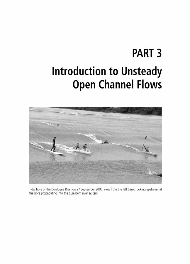
PART 3

Introduction to Unsteady Open Channel Flows

Tidal bore of the Dordogne River on 27 September 2000, view from the left bank, looking upstream atthe bore propagating into the quiescent river system.

This series of lectures is designed for undergraduate students in civil, environmental andhydraulic engineering, and professionals who want to expand their understanding of openchannel hydraulics. It will first develop the basic equations of unsteady open channel flows.That is, the Saint-Venant equations and the method of characteristics. Later, simple applicationsare developed. For example, the propagation of waves, positive and negative surges, the dambreak wave problem. At the end, simple numerical models are presented and explained.

Relevant Internet linkshttp://www.uq.edu.au/�e2hchans/photo.html#Tidal bores, Photographs of tidal boresmascaret, pororocahttp://www.uq.edu.au/�e2hchans/mascaret.html Tidal bore of the Seine

Riverhttp://boreriders.com/ Bore Riders Clubhttp://www.scvhistory.com/scvhistory/stfrancis.htm St Francis dam catastroph,

Santa Clarita ValleyHistorical Society

http://membres.lycos.fr/vitosweb/ Malpasset dam catastroph

11

Unsteady open channel flows:1. Basic equations

SummaryThe continuity and momentum equations are developed for one-dimensionalunsteady open channel flows. They yield the Saint-Venant equations. The basic assumptions are detailed and the method of characteristics is laterintroduced.

11.1 Introduction

Common examples of unsteady open channel flows includes flood flows in rivers and tidalflows in estuaries, irrigation channels, headrace and tailrace channel of hydropower plants,navigation canals, stormwater systems and spillway operation. Figure 11.1 illustrates extremeunsteady flow conditions. Figure 11.1(a) shows the upstream propagation of a tidal bore.Surfers give the scale of the phenomenon. Figure 11.1(b) presents a dam break wave propagat-ing down a flat stepped waterway.

In unsteady open channel flows (e.g. Fig. 11.1), the velocities and water depths change with time and longitudinal position. For one-dimensional applications, the relevant flow parameters (e.g. V and d) are functions of time and longitudinal distance.Analytical solutions of the basic equations are nearly impossible because of their non-linearity, but numerical techniques may provide approximate solutions for some specificcases.

The first major mathematical model of a river system was developed in J.J. Stoker for theOhio and Mississippi systems (Stoker 1953). It was followed by important developments inthe late 1950s in particular by A. Preissmann and J.A. Cunge in France. Mahmood andYevdjevich (1975) regrouped major contributions to the topic. Yevdjevich (1975) and Montes(1998, pp. 470–471) summarized the historical developments in numerical modelling ofunsteady open channel flows.

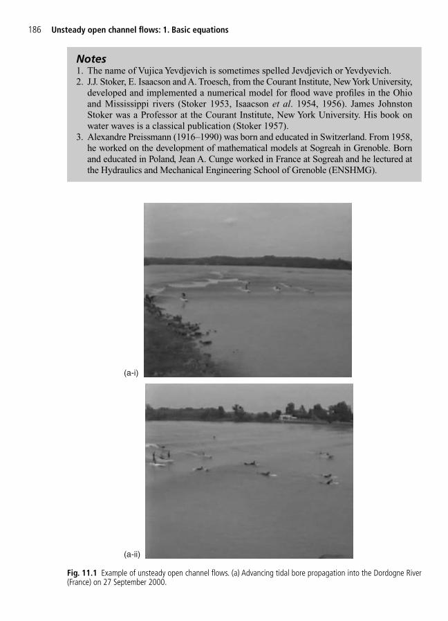
186 Unsteady open channel flows: 1. Basic equations

Notes1. The name of Vujica Yevdjevich is sometimes spelled Jevdjevich or Yevdyevich.2. J.J. Stoker, E. Isaacson and A. Troesch, from the Courant Institute, New York University,

developed and implemented a numerical model for flood wave profiles in the Ohioand Mississippi rivers (Stoker 1953, Isaacson et al. 1954, 1956). James JohnstonStoker was a Professor at the Courant Institute, New York University. His book onwater waves is a classical publication (Stoker 1957).

3. Alexandre Preissmann (1916–1990) was born and educated in Switzerland. From 1958,he worked on the development of mathematical models at Sogreah in Grenoble. Bornand educated in Poland, Jean A. Cunge worked in France at Sogreah and he lectured atthe Hydraulics and Mechanical Engineering School of Grenoble (ENSHMG).

(a-i)

Fig. 11.1 Example of unsteady open channel flows. (a) Advancing tidal bore propagation into the Dordogne River(France) on 27 September 2000.

(a-ii)

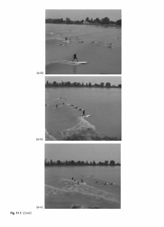
(a-v)

(a-iii)

Fig. 11.1 (Contd )

(a-iv)

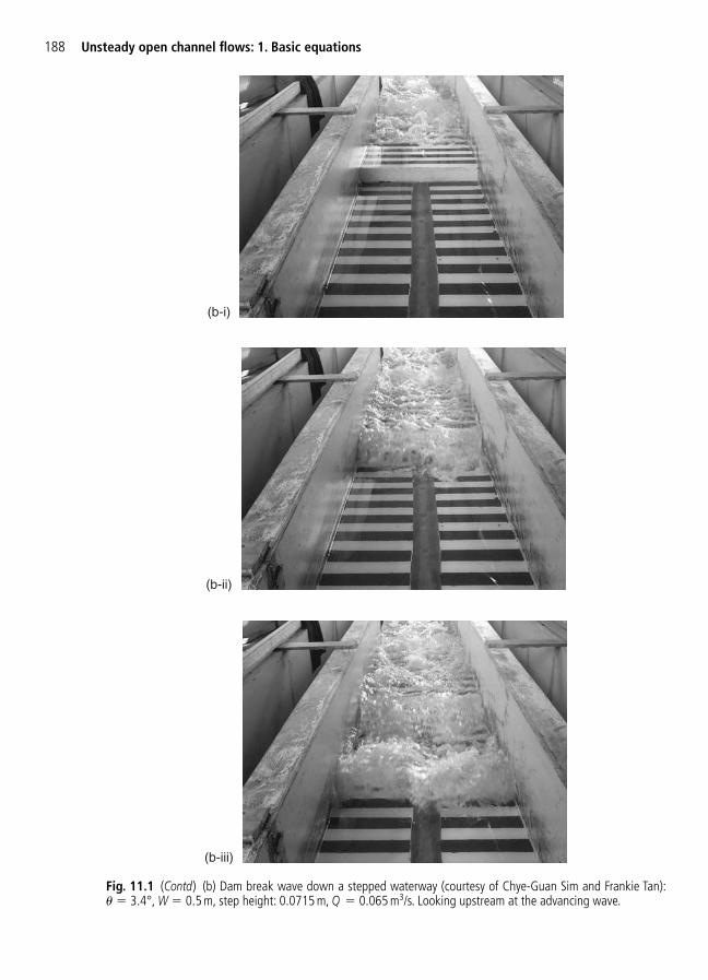
188 Unsteady open channel flows: 1. Basic equations

(b-i)

Fig. 11.1 (Contd) (b) Dam break wave down a stepped waterway (courtesy of Chye-Guan Sim and Frankie Tan):� � 3.4°, W � 0.5 m, step height: 0.0715 m, Q � 0.065 m3/s. Looking upstream at the advancing wave.

(b-ii)

(b-iii)

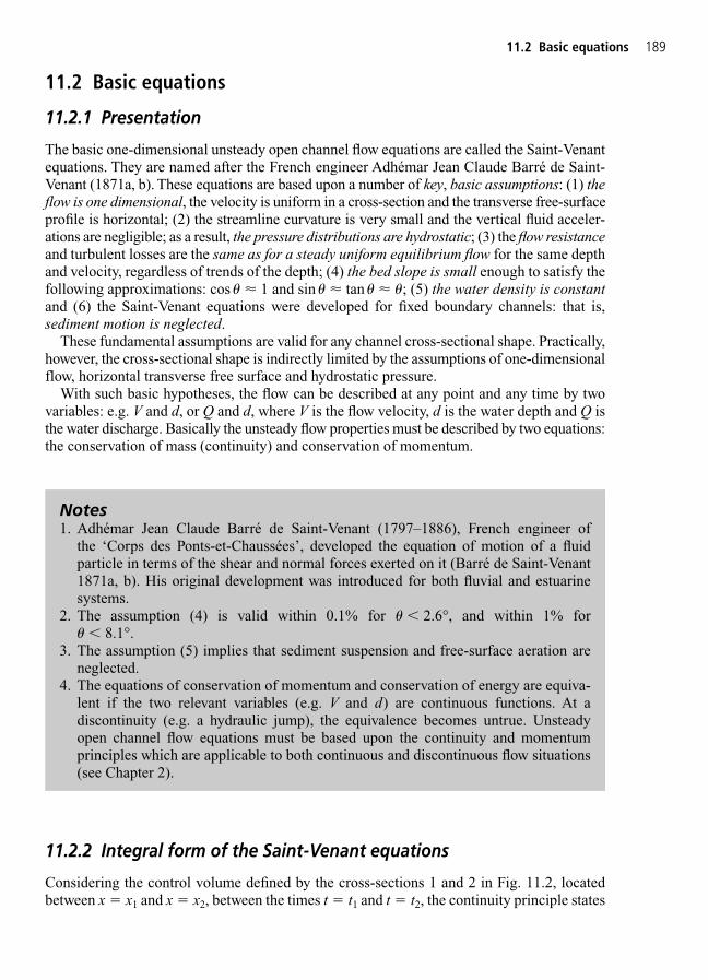
11.2 Basic equations 189

11.2 Basic equations

11.2.1 Presentation

The basic one-dimensional unsteady open channel flow equations are called the Saint-Venantequations. They are named after the French engineer Adhémar Jean Claude Barré de Saint-Venant (1871a, b). These equations are based upon a number of key, basic assumptions: (1) theflow is one dimensional, the velocity is uniform in a cross-section and the transverse free-surfaceprofile is horizontal; (2) the streamline curvature is very small and the vertical fluid acceler-ations are negligible; as a result, the pressure distributions are hydrostatic; (3) the flow resistanceand turbulent losses are the same as for a steady uniform equilibrium flow for the same depthand velocity, regardless of trends of the depth; (4) the bed slope is small enough to satisfy thefollowing approximations: cos � � 1 and sin � � tan � � �; (5) the water density is constantand (6) the Saint-Venant equations were developed for fixed boundary channels: that is, sediment motion is neglected.

These fundamental assumptions are valid for any channel cross-sectional shape. Practically,however, the cross-sectional shape is indirectly limited by the assumptions of one-dimensionalflow, horizontal transverse free surface and hydrostatic pressure.

With such basic hypotheses, the flow can be described at any point and any time by twovariables: e.g. V and d, or Q and d, where V is the flow velocity, d is the water depth and Q isthe water discharge. Basically the unsteady flow properties must be described by two equations:the conservation of mass (continuity) and conservation of momentum.

11.2.2 Integral form of the Saint-Venant equations

Considering the control volume defined by the cross-sections 1 and 2 in Fig. 11.2, locatedbetween x � x1 and x � x2, between the times t � t1 and t � t2, the continuity principle states

Notes1. Adhémar Jean Claude Barré de Saint-Venant (1797–1886), French engineer of

the ‘Corps des Ponts-et-Chaussées’, developed the equation of motion of a fluid particle in terms of the shear and normal forces exerted on it (Barré de Saint-Venant1871a, b). His original development was introduced for both fluvial and estuarinesystems.

2. The assumption (4) is valid within 0.1% for � � 2.6°, and within 1% for � � 8.1°.

3. The assumption (5) implies that sediment suspension and free-surface aeration areneglected.

4. The equations of conservation of momentum and conservation of energy are equiva-lent if the two relevant variables (e.g. V and d) are continuous functions. At a discontinuity (e.g. a hydraulic jump), the equivalence becomes untrue. Unsteadyopen channel flow equations must be based upon the continuity and momentum principles which are applicable to both continuous and discontinuous flow situations(see Chapter 2).

190 Unsteady open channel flows: 1. Basic equations

Fig. 11.2 Definition sketch: (a) side view, (b) top view and (c) cross-section.

d1d2

V1 V2

u

Datum

Y1 Y2

21

xFfric

Weight

x

zo2

zo1

(b)

(a)

d

Y

zoDatum

y

B

W

d – y

(c)

Fp1�

FpL�

Fp2�

Fp1� Fp2

�

FpR�

11.2 Basic equations 191

that the net mass flux into the control volume equals the net mass increase of the control volumebetween the times t1 and t2. Assuming no lateral inflow, it yields:

(11.1)

where � is the fluid density, V is the flow velocity, A is the flow cross-sectional area, the sub-scripts 1 and 2 refer to the upstream and downstream cross-sections respectively (Fig. 11.2), andthe subscripts t1 and t2 refer to the instants t � t1 and t � t2 respectively. Defining the total dis-charge Q � VA, and dividing equation (11.1) by the density �, the continuity equation becomes:

(11.2)

The application of the momentum equation in the x-direction states that the net change ofmomentum in the control volume between the instants t1 and t2 plus the rate of change ofmomentum flux across the volume equals the sum of the forces applied to the control volumein the x-direction. The net change of momentum in the control volume equals:

(11.3)

while the rate of change of momentum flux across the volume is equal to:

(11.4)

The forces acting on the control volume contained between sections 1 and 2 are the pressureforces at sections 1 and 2, the pressure force components on the channel sidewalls if thechannel width vary in the x-direction, the weight of the control volume, the reaction force ofthe bed (equal, in magnitude, to the weight in absence of vertical fluid motion) and the flowresistance opposing fluid motion. The pressure forces acting on sections 1 and 2 equal:

(11.5)

where

in which y is the distance measured from the bottom, d is the water depth and W is the channelwidth at the distance y above the bed (Fig. 11.2(c)).

When the channel width changes with distance, the pressure force components on the rightand left sidewalls equal:

(11.6)

where

Equation (11.6) states that, the water depth d being constant, an increase in wetted surfacein the x-direction induces a positive sidewall pressure force component. The above expression

I d yWx

yd

y2 0 d

constant

� �( )∫∂∂

=

( )F F t gI x tpt

tp x

x

t

tL R d d d� � �

1

2

1

2

1

2

2∫ ∫∫ �

I d y W yd

1 ( d0

� �∫ )

( ) (( ) ) )F F t I I tpt

tp t

t

11

2

2 1

2

1 1 1 2� �� � �∫ ∫ d ( d� �

(( ) ) )� �V A V A tt

t 21

22

1

2∫ ( d�

(( ) ) )� �VA VA xtx

xt11

2

2∫ ( d�

( ) (Q t A A xt

ttx

xt1

1

2

21

2

1 Q d ) d 02� � �∫ ∫

( ) (( )� � � �V A V A t A A xt

ttx

xt1 1 2 2

1

2

21

2 0 d ( ) ) d 1

� � �∫ ∫

of Fp� is valid only for gradual variations in cross-section. For sudden changes in cross-sectional

shapes, forces other than the hydrostatic pressure force take place.The gravity force component in the flow direction (i.e. x-direction) is:

(11.7)

where the bed slope So � sin � may be approximated to: So � tan � � �∂zo/∂x (assumption (4),Section 11.2.1).

Fluid motion is opposed by flow resistance and shear forces exerted on the wetted surfaces.The integration of the friction force Ffric between t � t1 and t � t2 is:

(11.8)

where Sf is the friction slope defined as:

(11.9)

�o is the average boundary shear stress, and DH is the hydraulic diameter.

SgDf

o

H

�4�

�

F t gAS x tt

t

x

x

t

tfric fd d d

1

2

1

2

1

2∫ ∫∫� �

�gAS x tx

x

t

to d d

1

2

1

2 ∫∫

192 Unsteady open channel flows: 1. Basic equations

Notes1. The momentum was called impetus by the Ancients. For example, Leonardo da Vinci

defined the impetus as: ‘Impetus is a power created by movement and transmittedfrom the mover to the movable thing; and this movable thing has as much movementas the impetus has life’ (McCurdy 1956, Vol. 1, p. 417). The term impetus as used byLeonardo da Vinci was a quantity proportional to the weight of the body and to itsvelocity (Levi 1995, p. 570). That is, the impetus was basically proportional to themomentum. Leonardo da Vinci added: ‘Impetus is (also) termed derived movement’(McCurdy 1956, Vol. 1, p. 523).

2. Leonardo da Vinci (AD 1452–1519) was an Italian artist who extended his interest tomedicine, science, engineering and architecture. In his notes, he described numerousflow situations and he commented the entrainment of air at waterfalls, plunging jetflows, drop structures, running waters and breaking waves (e.g. Chanson 1997a, pp. 327–329).

3. The momentum per unit volume equals �V. The momentum flux equals �VVA.4. The basic assumptions of the Saint-Venant equations (Section 11.2.1) imply that the

vertical pressure distribution is hydrostatic: i.e. P(y) � �g(d � y) for 0 " y " d.5. Simple geometrical considerations give:

where the free-surface width B and the flow cross-sectional area A are functions of bothdistance x and time t (Fig. 11.2).

W x y d t B x t

W y A

Ay

B

d( , , ) ( , )

d

� �

�

�

0∫∂∂

11.2 Basic equations 193

Combining equations (11.3) to (11.8), and dividing by the density � which is assumed tobe constant, the momentum equation becomes:

Equation (11.10) is the cross-sectional integration of the principle of momentum conservationfor one-dimensional unsteady open channel flows. It states that the net change of momentumin control volume (i.e. unsteady term) plus the rate of change of momentum flux across thevolume equal the pressure forces acting on sections 1 and 2, plus the pressure force componentson the right and left sidewalls, plus the gravity force component in flow direction and minusthe friction force Ffric acting on the wetted surface between t � t1 and t � t2.

Equations (11.2) and (11.10) form a system of two equations based upon the Saint-Venantequation assumptions (Section 11.2.1). They were developed without any additional assumptionand some characteristic parameter (e.g. V, A, d) might not be continuous. If one or more param-eter is discontinuous, equations (11.2) and (11.10) remain valid if the Saint-Venant hypothesesare respected.

11.2.3 Differential form of the Saint-Venant equations

The differential form of the Saint-Venant equations may be derived from the integral form(Section 11.2.2) if the relevant parameters are continuous and differentiable functions withrespect of x and y. The Taylor-series expansion of each parameter follows:

(11.11a)

(11.11b)

where �t � t2 � t1 and �x � x2 � x1. Neglecting the second order term, the continuityequation (11.2) yields:

(11.12)

Similarly the momentum principle (equation (11.10)) becomes:

(11.13)∂∂

∂∂

∂∂

∫∫ ∫∫Q

tV A

xt x g

Ix

I S S A t xt

t

x

x

t

t

x

x

(d d ( ) d do f � � � � �

21

21

2

1

2

1

2

1

2)

∂∂

∂∂

∫∫ A

tQx

t xt

t

x

x d d 0 �

1

2

1

2

Q QQx

xQ

x

x2 1

2

2

2

2

� ∂∂

∂∂

��

L

A AAt

tA

t

tt t2 1

2

2

� � ∂∂

∂∂

2

2�

L

(( ( ) ) d ( d

( d d d d d

2

2 2

o f

VA VA x V A V A t

I I t gI x t gA S S x t

tx

xt t

t

t

t

x

x

t

t

x

x

t

t

) (( ) ) )

(( ) ) ) ( )

11 2 1

2

1 1

2

1 1

2

1

2

21

22

1 1 1 2 2

∫ ∫∫ ∫∫ ∫∫

+� �

� � �

6. The left bank is located on the left-hand side of an observer when looking downstream.Conversely, the right bank is on the right-hand side of an observer looking downstream.

7. Yen (2002) discussed specifically the definitions of the friction slope. One series ofdefinitions is based upon the momentum principle (e.g. equation (11.9)) while theother is based upon the energy principle. All the definitions are equivalent for uniformequilibrium flow conditions.

(11.10)

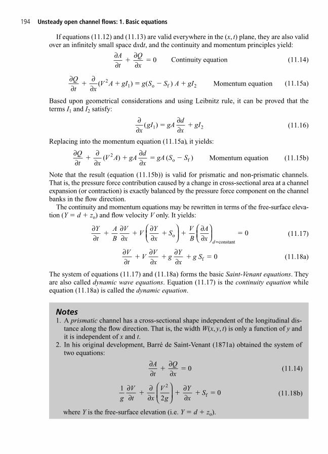
194 Unsteady open channel flows: 1. Basic equations

Notes1. A prismatic channel has a cross-sectional shape independent of the longitudinal dis-

tance along the flow direction. That is, the width W(x, y, t) is only a function of y andit is independent of x and t.

2. In his original development, Barré de Saint-Venant (1871a) obtained the system oftwo equations:

(11.14)

(11.18b)

where Y is the free-surface elevation (i.e. Y � d zo).

1

2 0

2

fgVt x

Vg

Yx

S∂∂

∂∂

∂∂

�

∂∂

∂∂

At

Qx

0 �

If equations (11.12) and (11.13) are valid everywhere in the (x, t) plane, they are also validover an infinitely small space dxdt, and the continuity and momentum principles yield:

Continuity equation (11.14)

Momentum equation (11.15a)

Based upon geometrical considerations and using Leibnitz rule, it can be proved that theterms I1 and I2 satisfy:

(11.16)

Replacing into the momentum equation (11.15a), it yields:

Momentum equation (11.15b)

Note that the result (equation (11.15b)) is valid for prismatic and non-prismatic channels.That is, the pressure force contribution caused by a change in cross-sectional area at a channelexpansion (or contraction) is exactly balanced by the pressure force component on the channelbanks in the flow direction.

The continuity and momentum equations may be rewritten in terms of the free-surface eleva-tion (Y � d zo) and flow velocity V only. It yields:

(11.17)

(11.18a)

The system of equations (11.17) and (11.18a) forms the basic Saint-Venant equations. Theyare also called dynamic wave equations. Equation (11.17) is the continuity equation whileequation (11.18a) is called the dynamic equation.

∂∂

∂∂

∂∂

Vt

VVx

gYx

g S f � 0

∂∂

∂∂

∂∂

∂∂

=

Yt

AB

Vx

VYx

SVB

Ax

d

oconstant

� 0

∂∂

∂∂

∂∂

Qt x

V A gAdx

gA S S o f � �( ) ( )2

∂∂

∂∂x

gI gAdx

gI( )1 2 �

∂∂

∂∂

Qt x

V A gI g S S A gI o f � � ( ) ( )21 2

∂∂

∂∂

At

Qx

0 �

DiscussionThe system of equations (11.2) and (11.10) is the integral form of the Saint-Venant equations,while the system of equations (11.17) and (11.18a) is the differential form of the Saint-Venantequations.

The systems of two equations formed by equations (11.2) and (11.10), and equations(11.17) and (11.18a), are equivalent if and only if all the variables and functions are continuous

11.2 Basic equations 195

3. Equation (11.18b) is dimensionless. The first term is related to the slope of flowacceleration energy line, the second term is the longitudinal slope of the kineticenergy line, the third one is the longitudinal slope of the free surface and the last termis the friction slope. In equation (11.18b), the two first terms are inertial terms. Insteady flows, the acceleration term ∂V/∂t is zero.

4. The Saint-Venant equations may be expressed in several ways. For example the con-tinuity equation may be written:

Note that equation (11.19) equals equation (11.17) if the cross-section varies slowlywith longitudinal distance which is one of the basic Saint-Venant assumptions.

The dynamic equation may be written:

All these equations are basically equivalent.

∂∂

∂∂

∂∂

∂∂

∂∂

∂∂

Qt x

V A gAdx

gA S S

gVt x

Vg

dx

S S

f o

f o

� �

� �

( ) ( )

( )

2

2

0

12

0

∂∂

∂∂

∂∂

∂∂

∂∂

∂∂

Vt

VVx

gYx

gS

Vt

VVx

gdx

g S S

f

f o

�

� �

0

0( )

∂∂

∂∂

∂∂

Yt

AB

Vx

VYx

S o � 0

∂∂

∂∂

∂∂

∂∂

∂∂

∂∂

∂∂

∂∂

=

=

Yt

AB

Vx

VYx

SVB

Ax

dt

AB

Vx

Vdx

VB

Ax

d

d

oconstant

constant

�

�

0

0

∂∂

∂∂

∂∂

∂∂

At

Qx

Bdt

Qx

�

�

0

0

(11.14)

(11.17)

(11.19)

(11.18a)

(11.15b)

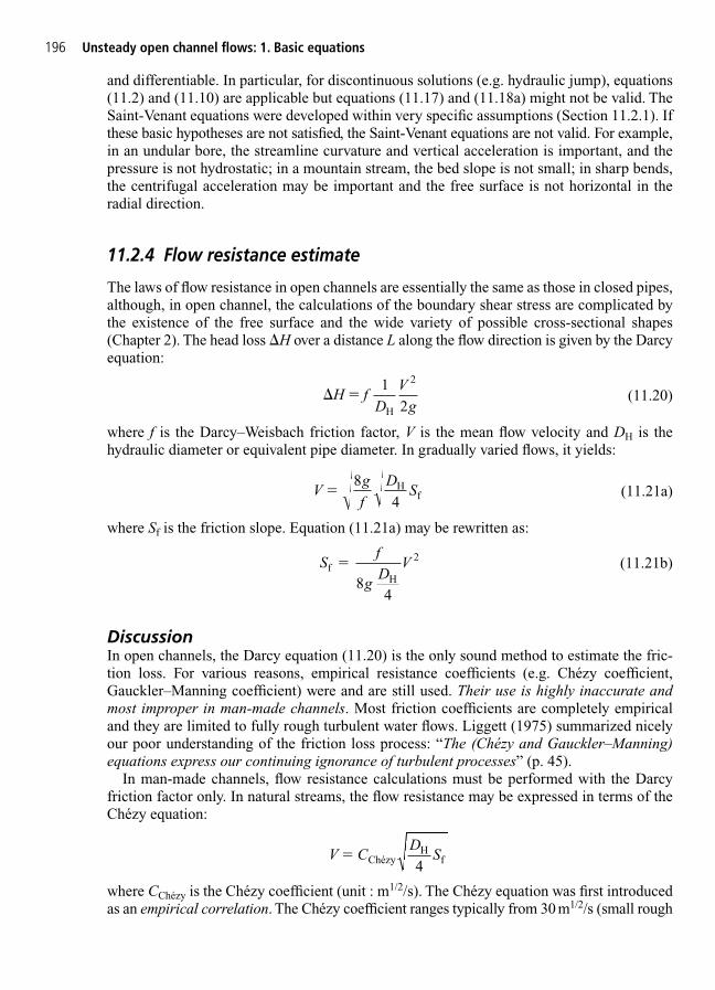
196 Unsteady open channel flows: 1. Basic equations

and differentiable. In particular, for discontinuous solutions (e.g. hydraulic jump), equations(11.2) and (11.10) are applicable but equations (11.17) and (11.18a) might not be valid. TheSaint-Venant equations were developed within very specific assumptions (Section 11.2.1). Ifthese basic hypotheses are not satisfied, the Saint-Venant equations are not valid. For example,in an undular bore, the streamline curvature and vertical acceleration is important, and thepressure is not hydrostatic; in a mountain stream, the bed slope is not small; in sharp bends,the centrifugal acceleration may be important and the free surface is not horizontal in theradial direction.

11.2.4 Flow resistance estimate

The laws of flow resistance in open channels are essentially the same as those in closed pipes,although, in open channel, the calculations of the boundary shear stress are complicated bythe existence of the free surface and the wide variety of possible cross-sectional shapes(Chapter 2). The head loss �H over a distance L along the flow direction is given by the Darcyequation:

(11.20)

where f is the Darcy–Weisbach friction factor, V is the mean flow velocity and DH is thehydraulic diameter or equivalent pipe diameter. In gradually varied flows, it yields:

(11.21a)

where Sf is the friction slope. Equation (11.21a) may be rewritten as:

(11.21b)

DiscussionIn open channels, the Darcy equation (11.20) is the only sound method to estimate the fric-tion loss. For various reasons, empirical resistance coefficients (e.g. Chézy coefficient,Gauckler–Manning coefficient) were and are still used. Their use is highly inaccurate andmost improper in man-made channels. Most friction coefficients are completely empiricaland they are limited to fully rough turbulent water flows. Liggett (1975) summarized nicelyour poor understanding of the friction loss process: “The (Chézy and Gauckler–Manning)equations express our continuing ignorance of turbulent processes” (p. 45).

In man-made channels, flow resistance calculations must be performed with the Darcyfriction factor only. In natural streams, the flow resistance may be expressed in terms of theChézy equation:

where CChézy is the Chézy coefficient (unit : m1/2/s). The Chézy equation was first introducedas an empirical correlation. The Chézy coefficient ranges typically from 30 m1/2/s (small rough

V CD

S ChézyH

f�4

Sf

gD

VfH

�

84

2

Vgf

DS H

f�8

4

�H fD

Vg

H

�1

2

2

channel) up to 90 m1/2/s (large smooth channel). Another empirical formulation, called theGauckler–Manning formula, was developed for turbulent flows in rough channels:

where nManning is the Gauckler–Manning coefficient (unit: s/m1/3). The Gauckler–Manningcoefficient is an empirical coefficient, found to be a function of the surface roughnessprimarily.

Vn

DS

Manning

Hf�

14

2 3

/

11.2 Basic equations 197

Remarks1. Henri Philibert Gaspard Darcy (1805–1858) was a French civil engineer. He performed

numerous experiments of flow resistance in pipes (Darcy 1858) and in open channels(Darcy and Bazin 1865), and of seepage flow in porous media (Darcy 1856). He gavehis name to the Darcy–Weisbach friction factor and to the Darcy law in porous media.

2. James A. Liggett is an Emeritus Professor in Fluid Mechanics at Cornell Universityand a former Editor of the Journal of Hydraulic Engineering.

3. The friction slope may be expressed as a function of the velocity as:

The hydraulic diameter equals four times the cross-sectional area divided by the wet-ted perimeter. For a wide rectangular channel, DH � 4A/Pw � 4d. The expressions ofthe friction slope yield then:

where |V | is the magnitude of the flow velocity. The friction has the same sign as thevelocity.

4. The conveyance (débitance in French) is defined as:

Conveyance o

�Q

S

Sfgd

V V

SC d

V V

Sn

dV V

f

fChézy

fManning

�

�

�

8

12

2

4 3

| |

| |

| |/

Sf

gD

V V

SC

DV V

Sn

DV V

fH

f

ChézyH

fManning

H

�

�

�

84

1

4

4

2

2

4 3

| |

| |

| |/

(11.21b)

(11.21c)

198 Unsteady open channel flows: 1. Basic equations

Flood plain calculationsConsidering a main channel with adjacent flood plains (Fig. 11.3), the flood plains and shallow-water zones are usually much rougher than the river channel. Assuming that the friction slopeof each portion is the same, the flow resistance may be estimated from:

(11.22)

where Q is the total discharge in the cross-section, Qi is the flow rate in the section {i}, andthe subscript i refers to the section {i}. Conversely, if the discharge, cross-sectional shape andfree-surface elevation are known, the friction slope may be estimated as:

(11.23)

where |Q| is the magnitude of the flow rate. Equation (11.23) is general and that it takes intoaccount the flow direction.

11.3 Method of characteristics

11.3.1 Introduction

The method of characteristics is a mathematical technique to solve a system of partial differen-tial equations such as the Saint-Venant equations. The differential form of the Saint-Venantequations may be expressed in terms of the water depth d:

(11.24)

(11.25)

where equations (11.24) and (11.25) are equivalent to equations (11.17) and (11.18a).Equation (11.24) is the continuity equation and equation (11.25) is the dynamic equation.

∂∂

∂∂

∂∂

Vt

VVx

gdx

g S S f o � �( ) 0

∂∂

∂∂

∂∂

∂∂

=

dt

AB

Vx

Vdx

VB

Ax

d

constant

� 0

SQ Q

gf

AD

ii

i

i

nf

H

�

�

| |

( )841

2

∑

Q Qgf

AD

Sii

n

ii

i

i

n

Hf� �

= =∑ ∑

1 1

84

( )

{i � 1} {i � 2} {i � 3} {i � 4}

Main channel

Fig. 11.3 Sketch of a flood plain cross-section (with four sections).

11.3 Method of characteristics 199

In an open channel, a small disturbance can propagate upstream and downstream. For arectangular channel, the celerity of a small disturbance equals: C � ��gd (Henderson 1966,Chanson 1999a, 2004b). In a channel of irregular cross-section, the celerity of a small wave is:C � �

__g(

__A/B

__), where A is the flow cross-section and B is the free-surface width (Fig. 11.2(c)).

The celerity C characterizes the propagation of a small disturbance (i.e. small wave) relativeto the fluid motion. For an observer standing on the bank, the absolute speed of the smallwave is (V C) and (V � C) where V is the flow velocity.

The differentiation of the celerity C with respect of time and of space satisfies respectively:

(11.26)

(11.27)

Replacing the terms ∂d/∂t and ∂d/∂x by equations (11.26) and (11.27) respectively in theSaint-Venant equations, it yields:

(11.28)

(11.29)

The addition of the two equations gives:

(11.30)

while the subtraction of equation (11.29) from equation (11.28) yields:

(11.31)

Equations (11.30) and (11.31) maybe rewritten as:

Forward characteristic (11.32a)

Backward characteristic (11.32b)

along their respective characteristic trajectories:

Forward characteristic C1 (11.33a)

Backward characteristic C2 (11.33b)

These trajectories are called characteristic directions or characteristics of the system. Foran observer travelling along the forward characteristics (Fig. 11.4, equation (11.33a)), equa-tion (11.32a) is valid at any point. For an observer travelling on the backward characteristics(equation 11.33b), equation (11.32b) is satisfied everywhere.

dd

xt

V C� �

dd

xt

V C�

DD

f otV C g S S( ) ( )� � � �2

DD

f otV C g S S( ) ( ) � � � �2 0

∂∂

∂∂

t

V Cx

V C g S S f o � � � �( ) ( ) ( )2 0

∂∂

∂∂

t

V Cx

V C g S S f o � �( ) ( ) ( )2 0

∂∂

∂∂

∂∂

Vt

CCx

VVx

g S S f o � �2 0( )

2 2 0∂∂

∂∂

∂∂

Ct

VCx

CVx

�

∂∂

∂∂

∂∂x

C CCx

gdx

( )2 2 � �

∂∂

∂∂

∂∂t

C CCt

gdt

( )2 2 � �

200 Unsteady open channel flows: 1. Basic equations

The system of four equations formed by equations (11.32) and (11.33) is equivalent to thesystem of equations (11.17) and (11.18a). These four equations represent the characteristicsystem of equations that replaces the differential form of the Saint-Venant equations. Thefamilies of forward (C1) and backward (C2) characteristics are shown in the (x, t) plane inFig. 11.4 for sub- and supercritical flows.

DiscussionThe absolute differential D/Dt of a scalar function �(x, t) equals:

where ∂x/∂t is the velocity. This yields:

Along a characteristic trajectory:

dd

xt

V C� �

DD

� � �

t tV

x�

∂∂

∂∂

DD

� � �

t txt x

� ∂∂

∂∂

∂∂

t

xx1

x1

x2

x2

Forwardcharacteristic

Backwardcharacteristic

dx

dt� V Cdx

dt � V � Cdxdt

t

x

t

x

Forwardcharacteristic

Backward characteristic

dx

dt

� V Cdxdt

� V � Cdxdt

(a)

(b)

Fig. 11.4 Definition sketch of the forward and backward characteristics: (a) subcritical flow conditions and(b) supercritical flow conditions.

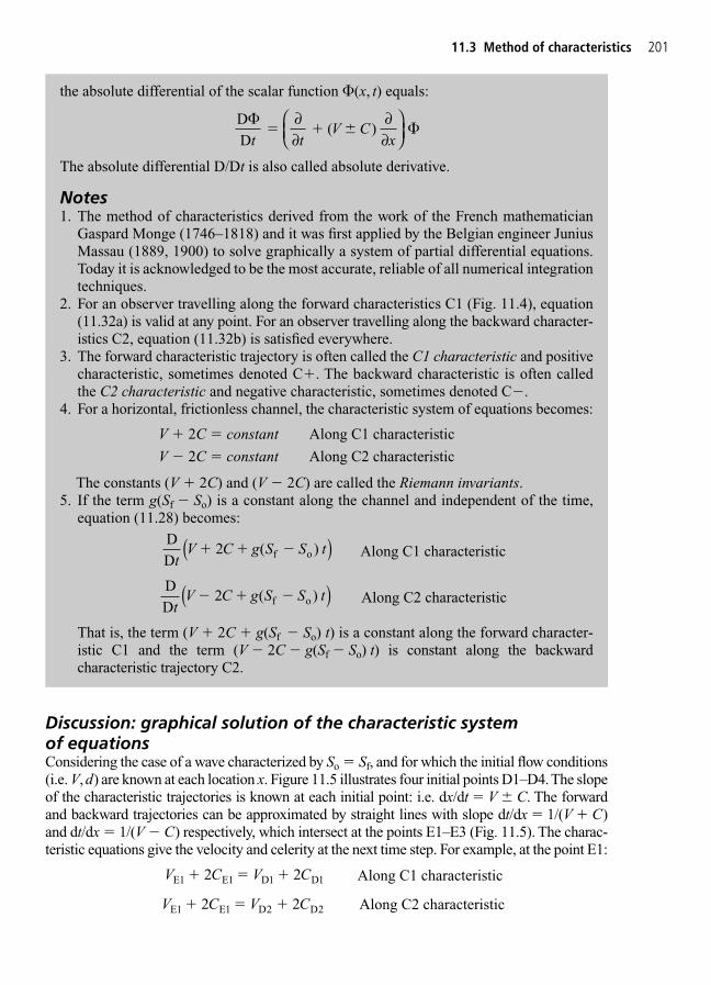
11.3 Method of characteristics 201

Discussion: graphical solution of the characteristic system of equationsConsidering the case of a wave characterized by So � Sf, and for which the initial flow conditions(i.e. V, d) are known at each location x. Figure 11.5 illustrates four initial points D1–D4. The slopeof the characteristic trajectories is known at each initial point: i.e. dx/dt � V � C. The forwardand backward trajectories can be approximated by straight lines with slope dt/dx � 1/(V C)and dt/dx � 1/(V � C) respectively, which intersect at the points E1–E3 (Fig. 11.5). The charac-teristic equations give the velocity and celerity at the next time step. For example, at the point E1:

Along C1 characteristic

Along C2 characteristicV C V CE E D D 1 1 2 22 2 �

V C V CE E D D 1 1 1 12 2 �

the absolute differential of the scalar function �(x, t) equals:

The absolute differential D/Dt is also called absolute derivative.

Notes1. The method of characteristics derived from the work of the French mathematician

Gaspard Monge (1746–1818) and it was first applied by the Belgian engineer JuniusMassau (1889, 1900) to solve graphically a system of partial differential equations.Today it is acknowledged to be the most accurate, reliable of all numerical integrationtechniques.

2. For an observer travelling along the forward characteristics C1 (Fig. 11.4), equation(11.32a) is valid at any point. For an observer travelling along the backward character-istics C2, equation (11.32b) is satisfied everywhere.

3. The forward characteristic trajectory is often called the C1 characteristic and positivecharacteristic, sometimes denoted C. The backward characteristic is often calledthe C2 characteristic and negative characteristic, sometimes denoted C�.

4. For a horizontal, frictionless channel, the characteristic system of equations becomes:

V 2C � constant Along C1 characteristic

V � 2C � constant Along C2 characteristic

The constants (V 2C) and (V � 2C) are called the Riemann invariants.5. If the term g(Sf � So) is a constant along the channel and independent of the time,

equation (11.28) becomes:

Along C1 characteristic

Along C2 characteristic

That is, the term (V 2C g(Sf � So) t) is a constant along the forward character-istic C1 and the term (V � 2C � g(Sf � So) t) is constant along the backward characteristic trajectory C2.

DD

f otV C g S S t� �2 ( )( )

DD

f otV C g S S t �2 ( )( )

DD

�

�t t

V Cx

� �∂∂

∂∂

( )

Similarly at E2 and E3, and then at F1, F2 and ultimately at G1. When the distance �x tends to zero, the graphical solution approaches the exact solution of the Saint-Venantequations.

In the example illustrated in Fig. 11.5, the flow properties at the point G1 are functions ofthe initial flow properties everywhere in the reach D1–D4. The interval D1–D4 is called theinterval of influence. In practice, an infinite number of characteristic curves crosses the intervalD1–D4 and the region D1–G1–D4 is called the domain of dependence for the point G1. Inthe computational process (Fig. 11.6), the properties of the point D2, whose initial conditionsare given, do influence a region delimited by the forward and backward characteristic trajector-ies through D2. This region is called the domain of influence (Fig. 11.6).

202 Unsteady open channel flows: 1. Basic equations

t

x

δ x δ x

D1 D2 D3 D4

E1 E2 E3

F1 F2

G1

Domainof dependence

Fig. 11.5 Network of characteristic trajectories and domain of dependence.

t

x

δx

D1 D2

E1Domain

of dependence

Backward characteristicForward characteristic

Domain ofinfluence

Fig. 11.6 Sketch of the region of influence.

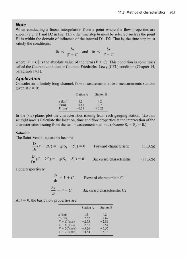
11.3 Method of characteristics 203

NoteWhen conducting a linear interpolation from a point where the flow properties areknown (e.g. D1 and D2 in Fig. 11.5), the time step �t must be selected such as the pointE1 is within the domain of influence of the interval D1–D2. That is, the time step mustsatisfy the conditions:

where |V C | is the absolute value of the term (V C). This condition is sometimescalled the Courant condition or Courant–Friedrichs–Lewy (CFL) condition (Chapter 14,paragraph 14.1).

ApplicationConsider an infinitely long channel, flow measurements at two measurements stationsgiven at t � 0:

Station A Station B

x (km) 1.5 4.2d (m) 0.65 0.73V (m/s) 0.21 0.22

In the (x, t) plane, plot the characteristics issuing from each gauging station. (Assumestraight lines.) Calculate the location, time and flow properties at the intersection of thecharacteristics issuing from the two measurement stations. (Assume Sf � So � 0.)

SolutionThe Saint-Venant equations become:

Forward characteristic (11.32a)

Backward characteristic (11.32b)

along respectively:

Forward characteristic C1

Backward characteristic C2

At t � 0, the basic flow properties are:

Station A Station B

x (km) 1.5 4.2C (m/s) 2.52 2.67V C (m/s) 2.73 2.89V � C (m/s) �2.31 �2.54V 2C (m/s) 5.26 5.57V � 2C (m/s) �4.84 �5.13

dd

xt

V C� �

dd

xt

V C�

DD

f otV C g S S( ) ( )� � � � �2 0

DD

f otV C g S S( ) ( ) � � � �2 0

� "�

� "

�

�t

xV C

tx

V C

and

| | | |

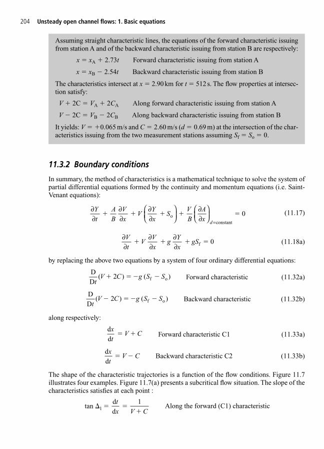
204 Unsteady open channel flows: 1. Basic equations

11.3.2 Boundary conditions

In summary, the method of characteristics is a mathematical technique to solve the system ofpartial differential equations formed by the continuity and momentum equations (i.e. Saint-Venant equations):

(11.17)

(11.18a)

by replacing the above two equations by a system of four ordinary differential equations:

Forward characteristic (11.32a)

Backward characteristic (11.32b)

along respectively:

Forward characteristic C1 (11.33a)

Backward characteristic C2 (11.33b)

The shape of the characteristic trajectories is a function of the flow conditions. Figure 11.7illustrates four examples. Figure 11.7(a) presents a subcritical flow situation. The slope of thecharacteristics satisfies at each point :

Along the forward (C1) characteristictan dd

1

�1 � �

tx V C

dd

xt

V C� �

dd

xt

V C�

DD

f otV C g S S( ) ( )� � � �2

DD

f otV C g S S( ) ( ) � � �2

∂∂

∂∂

∂∂

Vt

VVx

gYx

gS f � 0

∂∂

∂∂

∂∂

∂∂

=

Yt

AB

Vx

VYx

SVB

Ax

d

oconstant

� 0

Assuming straight characteristic lines, the equations of the forward characteristic issuingfrom station A and of the backward characteristic issuing from station B are respectively:

x � xA 2.73t Forward characteristic issuing from station A

x � xB � 2.54t Backward characteristic issuing from station B

The characteristics intersect at x � 2.90 km for t � 512 s. The flow properties at intersec-tion satisfy:

V 2C � VA 2CA Along forward characteristic issuing from station A

V � 2C � VB � 2CB Along backward characteristic issuing from station B

It yields: V � 0.065 m/s and C � 2.60 m/s (d � 0.69 m) at the intersection of the char-acteristics issuing from the two measurement stations assuming Sf � So � 0.

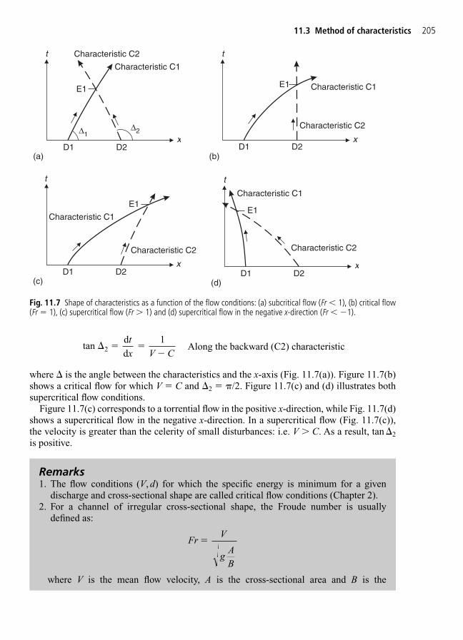
Along the backward (C2) characteristic

where � is the angle between the characteristics and the x-axis (Fig. 11.7(a)). Figure 11.7(b)shows a critical flow for which V � C and �2 � �/2. Figure 11.7(c) and (d) illustrates bothsupercritical flow conditions.

Figure 11.7(c) corresponds to a torrential flow in the positive x-direction, while Fig. 11.7(d)shows a supercritical flow in the negative x-direction. In a supercritical flow (Fig. 11.7(c)),the velocity is greater than the celerity of small disturbances: i.e. V � C. As a result, tan �2is positive.

tan dd

1

�2 � �

�

tx V C

11.3 Method of characteristics 205

t

xD1 D2

E1

Characteristic C1

Characteristic C2

∆1∆2

(a)

Characteristic C1

Characteristic C2

t

xD1 D2

E1

(b)

Characteristic C1

Characteristic C2

t

xD1 D2

E1

(c)

Characteristic C1

Characteristic C2

t

xD1 D2

E1

(d)

Fig. 11.7 Shape of characteristics as a function of the flow conditions: (a) subcritical flow (Fr � 1), (b) critical flow(Fr � 1), (c) supercritical flow (Fr � 1) and (d) supercritical flow in the negative x-direction (Fr � �1).

Remarks1. The flow conditions (V, d) for which the specific energy is minimum for a given

discharge and cross-sectional shape are called critical flow conditions (Chapter 2).2. For a channel of irregular cross-sectional shape, the Froude number is usually

defined as:

where V is the mean flow velocity, A is the cross-sectional area and B is the

FrV

gAB

�

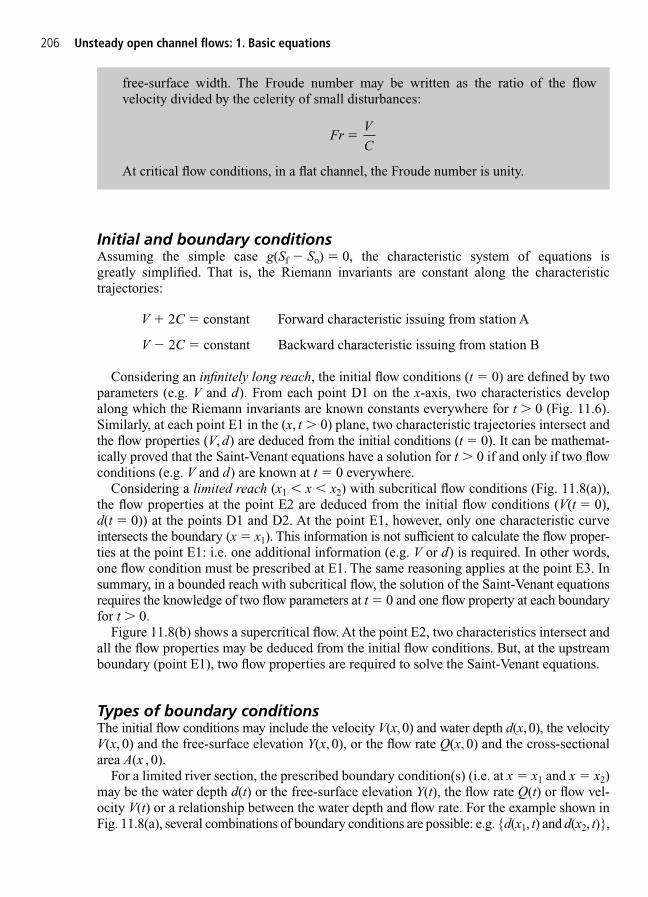
Initial and boundary conditionsAssuming the simple case g(Sf � So) � 0, the characteristic system of equations isgreatly simplified. That is, the Riemann invariants are constant along the characteristictrajectories:

V 2C � constant Forward characteristic issuing from station A

V � 2C � constant Backward characteristic issuing from station B

Considering an infinitely long reach, the initial flow conditions (t � 0) are defined by twoparameters (e.g. V and d). From each point D1 on the x-axis, two characteristics developalong which the Riemann invariants are known constants everywhere for t � 0 (Fig. 11.6).Similarly, at each point E1 in the (x, t � 0) plane, two characteristic trajectories intersect andthe flow properties (V, d) are deduced from the initial conditions (t � 0). It can be mathemat-ically proved that the Saint-Venant equations have a solution for t � 0 if and only if two flowconditions (e.g. V and d) are known at t � 0 everywhere.

Considering a limited reach (x1 � x � x2) with subcritical flow conditions (Fig. 11.8(a)),the flow properties at the point E2 are deduced from the initial flow conditions (V(t � 0),d(t � 0)) at the points D1 and D2. At the point E1, however, only one characteristic curveintersects the boundary (x � x1). This information is not sufficient to calculate the flow proper-ties at the point E1: i.e. one additional information (e.g. V or d) is required. In other words,one flow condition must be prescribed at E1. The same reasoning applies at the point E3. Insummary, in a bounded reach with subcritical flow, the solution of the Saint-Venant equationsrequires the knowledge of two flow parameters at t � 0 and one flow property at each boundaryfor t � 0.

Figure 11.8(b) shows a supercritical flow. At the point E2, two characteristics intersect andall the flow properties may be deduced from the initial flow conditions. But, at the upstreamboundary (point E1), two flow properties are required to solve the Saint-Venant equations.

Types of boundary conditionsThe initial flow conditions may include the velocity V(x, 0) and water depth d(x, 0), the velocityV(x, 0) and the free-surface elevation Y(x, 0), or the flow rate Q(x, 0) and the cross-sectionalarea A(x , 0).

For a limited river section, the prescribed boundary condition(s) (i.e. at x � x1 and x � x2)may be the water depth d(t) or the free-surface elevation Y(t), the flow rate Q(t) or flow vel-ocity V(t) or a relationship between the water depth and flow rate. For the example shown inFig. 11.8(a), several combinations of boundary conditions are possible: e.g. {d(x1, t) and d(x2, t)},

206 Unsteady open channel flows: 1. Basic equations

free-surface width. The Froude number may be written as the ratio of the flow velocity divided by the celerity of small disturbances:

At critical flow conditions, in a flat channel, the Froude number is unity.

FrVC

�

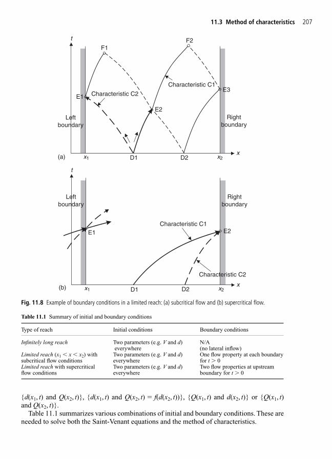
{d(x1, t) and Q(x2, t)}, {d(x1, t) and Q(x2, t) � f(d(x2, t))}, {Q(x1, t) and d(x2, t)} or {Q(x1, t) and Q(x2, t)}.

Table 11.1 summarizes various combinations of initial and boundary conditions. These areneeded to solve both the Saint-Venant equations and the method of characteristics.

11.3 Method of characteristics 207

t

D1 D2

E1

E2

E3

F1F2

Rightboundary

Leftboundary

x1 x2

Characteristic C2

Characteristic C1

x(a)

t

D1 D2

E1 E2

x1 x2

Characteristic C2

Characteristic C1

x

Rightboundary

Leftboundary

(b)

Fig. 11.8 Example of boundary conditions in a limited reach: (a) subcritical flow and (b) supercritical flow.

Table 11.1 Summary of initial and boundary conditions

Type of reach Initial conditions Boundary conditions

Infinitely long reach Two parameters (e.g. V and d) N/Aeverywhere (no lateral inflow)

Limited reach (x1 � x � x2) with Two parameters (e.g. V and d) One flow property at each boundarysubcritical flow conditions everywhere for t � 0Limited reach with supercritical Two parameters (e.g. V and d) Two flow properties at upstreamflow conditions everywhere boundary for t � 0

11.3.3 Application: numerical integration of the method of characteristics

The characteristic system of equations may be regarded as the conservation of basic flowproperties (velocity, celerity) when viewed by observers travelling on the characteristic trajecto-ries. At each intersection of forward and backward characteristics, there are four unknowns(x, t, V, C) which are the solution of the system of four differential equations. Such a solutionis however impossible at a flow discontinuity (e.g. surge front).

The characteristic system of equations may be numerically integrated. Ideally a variablegrid of point may be selected in the (x, t) plane where each point (x, t) is the crossing of twocharacteristics: i.e. a forward characteristic and a backward characteristic. The variable gridmethod requires however two types of interpolation because (1) the hydraulic and geometricproperties of the channel are defined only at a limited number of sections and (2) the computedresults are found at a number of (x, t) points unevenly distributed in the domain. In practice,a fixed grid method is preferred by practitioners: i.e. the Hartree method.

The Hartree scheme uses fixed time and spatial intervals (Fig. 11.9). The flow propertiesare known at the time t � (n � 1) �t. At the following time step t �t, the characteristicsintersecting at point M (x � i �x, t � n �t) are projected backward in time where they intersectthe line t � (n � 1) �t at points L and R whose locations are unknown (Fig. 11.9). Since xLand xR do not coincide with grid points, the velocity and celerity at points R and L must

208 Unsteady open channel flows: 1. Basic equations

DISCUSSIONIt is impossible to set Q(x1, t) � F(d(x � 0, t)) unless critical flow conditions occur at theupstream boundary section (x � x1).

For a set of boundary conditions {Q(x1, t) and Q(x2, t)}, the particular case Q(x1, t) �Q(x2, t) implies that the inflow equals the outflow. The mass of water does not change andthe variations of the free surface is strongly affected by the initial conditions.

t

x

δx δx

(i �1) δx i δx (i 1) δx

(n � 1) δt

n δt

(n 1) δt

δt

δt

C2 characteristicC1 characteristic

L

M

A B CR

Fig. 11.9 Numerical integration of the method of characteristics by the Hartree method.

be interpolated between x � (i � 1) �x and x � i �x, and between x � i �x and x � (i 1)�xrespectively. The discretization of the characteristic system of equations gives:

Forward characteristic (11.34a)

Backward characteristic (11.34b)

Forward characteristic (11.34c)

Backward characteristic (11.34d)

assuming (Sf � So) constant during the time step �t. The system of four equations has fourunknowns: VM and CM, and xL and xR, where the subscripts M, L and R refer respectively topoints M, L and R defined in Fig. 11.9.

The stability of the solution of the method of characteristics is based upon the Courantcondition. That is, the time step �t and the interval length �x must satisfy:

where V is the flow velocity and C is the small wave celerity.The solution of the Hartree scheme is artificially smoothened by interpolation errors to

estimate the flow conditions (V, C) at points L and R. The errors are cumulative with time andthe resulting inaccuracy limits the applicability of the method. In practice, finite differencemethods offer many improvement in accuracy: e.g., Lax diffusive scheme, Preissmann-Cungemethod (Chapter 14).

| |1 and

| |1

V Cxt

V Cxt

�

�

"�

�

�

"

x xt

V CM RR R

�

��

x xt

V CM LL L

�

��

V C V C g S S tR R M M f o 2 2 � � � � �( )

V C V C g S S tL L M M f o 2 2 � � �( )

11.3 Method of characteristics 209

Notes1. The Hartree method was named after the English physicist Douglas R. Hartree

(1897–1958). The Hartree approximation to the Schrödinger equation is the basis forthe modern physical understanding of the wave mechanics of atoms. The scheme issometimes called the Hartree–Fock method after the Russian physicist V. Fock whogeneralized Hartree’s scheme.

2. In open channel flows, the Hartree method is also called the method of specified timeintervals.

3. When the flow properties at points L and R are linearly interpolated between pointsA and B, and between points B and C respectively (Fig. 11.9), it yields

CC

tx

V C C

tx

C CL

B L A B

B A

( )

( )�

�

��

�

��1

VV

tx

C V C V

tx

V C V CL

B B A A B

B B A A

( )

�

�

��

�

� � �1 ( )

210 Unsteady open channel flows: 1. Basic equations

If the term (Sf � So) is estimated at points L and R, the discretization of the character-istic system of equations gives:

Note that the equations were derived assuming subcritical flow conditions as illustratedin Fig. 11.9. The interpolations have to be re-derived for supercritical flow conditions.

4. The above development based upon a linear interpolation was first proposed by Courantet al. (1952). A more accurate method is the parabolic interpolation presented byMontes (1998, pp. 492–495).

ApplicationA 2 km long irrigation channel is supplied by a large reservoir and controlled by a down-stream radial gate (Fig. 11.10(a)). During a gate operation, the flow velocity, immediatelyupstream of the gate, increases linearly from 0 to 1 m/s in 2 min. The channel is concretelined (f � 0.015), rectangular (W � 12 m), the invert slope is zero, and the water depth ismaintained constant (d � 2 m) at the canal intake. Calculate the water depths at thedownstream gate, at mid-distance and at the canal intake for the next 10 min.

DiscussionInitially the water in the canal is at rest and the free-surface elevation is that in the upstreamreservoir.

Let select the x-direction positive in the downstream direction with x � 0 at the canal intakeand x � 2000 m at the gate. The time origin (t � 0) is taken at the start of gate operation.

For t � 0, the boundary conditions are:

• constant depth at the upstream end and• given flow velocity at the downstream end (i.e. gate).

At the upstream boundary, the flow velocity V is deduced from:

Backward characteristic

where C is deduced from the imposed water depth.At the downstream boundary, the flow depth is calculated from:

Forward characteristic

where the flow velocity V is known.

V C V C g S S tL L F o 2 2 � � �( )

V C V C g S S tR R f o 2 2 � � � � �( )

C V V C C g tS S S S

M L R L Rf L f R o L o R

14

2( ) 2 2

2

� � � ��

��( ) ( ) ( ) ( )

V V V C C g tS S S S

M L R L Rf L f R o L o R

12

2( ) 2 2

2

� � � �

�( ) ( ) ( ) ( )

CC

tx

V C C

tx

C CR

B R B C

B C

( )

( )�

�

��

�

��1

VV

tx

C V C V

tx

V C V CR

B B C C B

C C B B

( )

( )�

�

��

�

� � �1

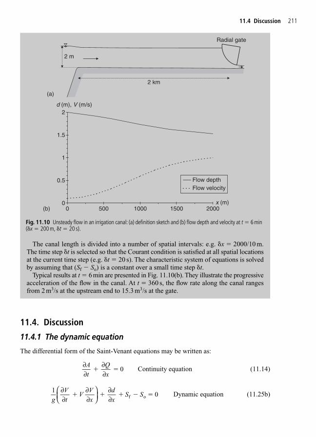
11.4. Discussion

11.4.1 The dynamic equation

The differential form of the Saint-Venant equations may be written as:

Continuity equation (11.14)

Dynamic equation (11.25b)1g

Vt

VVx

dx

S S∂∂

∂∂

∂∂

0f o � �

∂∂

∂∂

At

Qx

0 �

11.4 Discussion 211

The canal length is divided into a number of spatial intervals: e.g. �x � 2000/10 m.The time step �t is selected so that the Courant condition is satisfied at all spatial locationsat the current time step (e.g. �t � 20 s). The characteristic system of equations is solvedby assuming that (Sf � So) is a constant over a small time step �t.

Typical results at t � 6 min are presented in Fig. 11.10(b). They illustrate the progressiveacceleration of the flow in the canal. At t � 360 s, the flow rate along the canal rangesfrom 2 m3/s at the upstream end to 15.3 m3/s at the gate.

Radial gate

2 m

2 km

(a)

Flow depthFlow velocity

0

0.5

1

1.5

2

0

d (m), V (m/s)

(b) 500 1000 1500 2000x (m)

Fig. 11.10 Unsteady flow in an irrigation canal: (a) definition sketch and (b) flow depth and velocity at t � 6 min(�x � 200 m, �t � 20 s).

For steady flows, the continuity equation states ∂Q/∂x � 0 (i.e. constant flow rate) in absenceof lateral inflow and the dynamic equation yields:

Steady flows (11.34)

Equation (11.34) is basically the backwater equation for flat channels (Chapter 2, paragraph2.5.3) and it may be rewritten as:

Steady flows (11.34b)

where � is the momentum correction coefficient which is assumed a constant (Henderson1966, Chanson 1999a). Note a major difference between the backwater equation and equation(11.34b). The former derives from the energy equation but the latter was derived from themomentum principle.

For steady uniform equilibrium flows, the dynamic equation yields:Steady uniform equilibrium flows (11.35)

Simplification of the dynamic wave equation for unsteady flowsIn the general case of unsteady flows, the dynamic equation (11.25b) may be simplified undersome conditions, if the acceleration term ∂V/∂t and the inertial term V(∂V/∂x) become small.For example, when the flood flow velocity increases from 1 to 2 m/s in 3 h (i.e. rapid varia-tion), the dimensionless acceleration term (1/g)(∂V/∂t) equals 9.4 � 10�6; when the velocityincreases from 1.0 to 1.4 m/s along a 10 km reach (e.g. reduction in channel width), the lon-gitudinal slope of the kinetic energy line (1/g)V(∂V/∂x) is equal to 4.9 � 10�6. For compari-son, the average bed slope So of the Rhône River between Lyon and Avignon (France) isabout 0.7 � 10�3 and the friction slope is of the same order of magnitude; the average bedslope and friction slope of the Tennessee River between Watts Bar and Chickamaugo Dam is0.22 � 10�3; during a flood in the Missouri River, the discharge increased very rapidly from680 to 2945 m3/s, but the acceleration term was �5% of the friction slope; on the KitakamiRiver (Japan), actual flood records showed that the dimensionless acceleration and inertialterms were �1.5% than the term ∂d/∂x (Miller and Cunge 1975, p. 189).

The dynamic equation may be simplified when some terms become negligible. Table 11.2summarises various forms of the dynamic wave equation which may be solved in combination

S Sf o 0� �

∂∂

dx

V

gAB

S S1 2

o f� � ��

∂∂

∂∂

dx g

VVx

S S 1

0f o � �

212 Unsteady open channel flows: 1. Basic equations

Table 11.2 Simplification of the dynamic wave equation

Equation Dimensionless expression Remarks(1) (2) (3)

Dynamic wave Saint-Venant equationequation

Diffusive wave See Chapter 12, paragraph 12.6.equation

Kinematic wave See Chapter 12, paragraph 12.5 equation and Chapter 13.

∂∂d

xS S 0f o � �

0f oS S� �

1 0f og

V

tV

V

x

d

xS S

∂∂

∂∂

∂∂

� �

with the unsteady flow continuity equation (Eq. (11.14)). Applications are presented inChapters 12 and 13.

11.4.2 Limitations of the Saint-Venant equations

The Saint-Venant equations were developed for one-dimensional flows with hydrostatic pressuredistributions, small bed slopes, constant water density, no sediment motion and assuming thatthe flow resistance is the same as for a steady uniform flow for the same depth and velocity.

Limitations of the Saint-Venant equation applications include two- and three-dimensionalflows, shallow-water flood plains where the flow is nearly two-dimensional, undular and wavyflows, and the propagation of sharp discontinuities. Overall the assumptions behind the Saint-Venant equations are very restrictive and limit their applicability.

Flood plainsIn two-dimensional problems involving flood propagation over inundated plains (Fig. 11.11(a)),the flood build-up is relatively slow, except when dykes break. The resistance terms are thedominant term in the dynamic equation. The assumption of one-dimensional flow becomesinaccurate.

Cunge (1975b) proposed an extension of the Saint-Venant equation in which flood plainsare considered as storage volumes and with a system of equations somehow comparable to anetwork analysis.

Non-hydrostatic pressure distributionsThe Saint-Venant equations are inaccurate when the flow is not one-dimensional and thepressure distributions are not hydrostatic. Examples include flows in sharp bends, undularhydraulic jumps, undular tidal bores (Fig. 11.11(b)). Other relevant situations include super-critical flows with shock waves, flows over a ski jump.

Sharp discontinuitiesThe differential form of the Saint-Venant equations does not apply across sharp discontinuities.Figure 11.11(c) and (d) illustrates two examples: a hydraulic jump in a channelized stream

11.4 Discussion 213

Remarks1. Undular bores (and surges) are positive surge characterized by a train of secondary

waves (or undulations) following the surge front (Fig. 11.11(b)). They are calledBoussinesq–Favre waves in homage to the contributions of J.B. Boussinesq and H. Favre. Classical studies of undular surges include Benet and Cunge (1971) and Treske (1994). Frazao and Zech (2002) and Cunge (2003) presented a pertinentdiscussion of the application of Saint-Venant equations to undular surges.

2. With supercritical flows, a flow disturbance (e.g. change of direction, contraction)induces the development of shock waves propagating at the free surface across thechannel (e.g. Ippen and Harleman 1956). Shock waves are also called lateral shockwaves, oblique hydraulic jumps, Mach waves, crosswaves, diagonal jumps. They induceflow concentrations. They create a local discontinuity in terms of water depth andpressure distributions.

214 Unsteady open channel flows: 1. Basic equations

(a)

(b)

Fig. 11.11 Example of flow situations where the Saint-Venant equations are not applicable. (a) Flood of the SeineRiver at Duclair (15 km between Rouen and Caudebec, France) on 28 March 2001 (courtesy of Ms Nathalie Lemiere,Sequana-Normandie). The flooding was inflated by spring tides (coefficient 91) and strong winds. Looking down-stream, note the barge and ferry attached to the quay. (b) Undular tidal bore in the Salmon River, Truro, Canada on22 September 2001 (courtesy of Dr M.R. Gourlay).

11.4 Discussion 215

(c)

(d)

Fig. 11.11 (Contd) (c) Hydraulic jump roller in a steep stream in Münich, English garden in August 2002 (courtesyof Ms Sasha Kurz), flow from bottom to top. (d) Small overflow over a stepped weir at Robina, Gold Coast on 3 February 2003.

and a weir. At a hydraulic jump, the momentum equation must be applied across the jumpfront (Fig. 11.11(c)). At the weir crest, the Bernoulli equation may be applied (Fig. 11.11(d)).If the weir becomes submerged, the structure acts as a large roughness and a singularenergy loss.

RemarksAnother example of sharp transition is a sudden channel contraction. Assuming a smoothand short transition, the Bernoulli principle implies conservation of total head. Barnett(2002) discussed errors induced by the Saint-Venant equations for the triangular channelcontraction.

RemarksFigure 11.11(e) and (f) presents further flow situations when the Saint-Venant equations arenot applicable. Figure 11.11(e) shows massive sediment motion in a Japanese river that leadto rapid reservoir siltation. Figure 11.11(f) illustrates free-surface aeration down a steep chute,while, at the chute toe, further air is entrapped at the discontinuity between the high-velocityflow and the receiving pool of water. For such a flow, the fluid density is not a constant andthe Saint-Venant equations cannot be applied.

216 Unsteady open channel flows: 1. Basic equations

(e)

(f)

Fig. 11.11 (Contd ) (e) Extreme siltation of the Nishiyawa Dam Reservoir on the Hayakawa River (Japan, 1957) –looking at the dam wall in background with the fully silted reservoir in the foreground in November 1998. The reser-voir became fully silted by gravel bed load in �20 years. It was dredged around 1988 (2 m depth) to resume hydro-electricity production. (f) Air entrainment at Chinchilla weir (Australia). Note self-aeration down chute and in hydraulic jump (foreground). The beige colour of water is caused by three-phase mixing (air, water and sediment).

11.4.3 Summary

The Saint-Venant equations are the unsteady flow equivalent of the backwater equation. Thelatter was developed for steady gradually varied flows (Chapter 2) and it is derived from theenergy equation, while the Saint-Venant equations are derived from the momentum equation.Both the backwater and Saint-Venant equations are developed for one-dimensional flows,assuming a hydrostatic pressure distribution, for gradually varied flows, neglecting sedimenttransport and assuming that the flow resistance is the same as for uniform equilibrium flowconditions for the same depth and velocity. The Saint-Venant equations assume further thatthe slope is small. Note that the backwater equation may account for the bed slope (Chapter 2)and a pressure correction coefficient may be introduced if the pressure is not hydrostatic(Henderson 1966, Chanson 1999a, 2004b).

The assumptions behind the Saint-Venant equations are very restrictive and limit the applic-ability of the results (see Section 11.4.2). Professor Liggett concluded: “in the end it is neces-sary to ‘calibrate’any mathematical model against field data before confidence can be placedin the computations” (Liggett 1994, p. 305).

11.5 Exercises

1. Write the five basic assumptions used to develop the Saint-Venant equations.2. Were the Saint-Venant equations developed for movable boundary hydraulic

situations?3. Are the Saint-Venant equations applicable to a steep slope?4. Express the differential form of the Saint-Venant equations in terms of the water depth

and flow velocity. Compare the differential form of the momentum equation with the back-water equation.

5. What is the dynamic wave equation? From which fundamental principle does it derive?6. What are the two basic differences between the dynamic wave equation and the backwater

equation?

11.5 Exercises 217

DISCUSSIONAir entrainment, or free-surface aeration, is defined as the entrainment/entrapment of un-dissolved air bubbles and air pockets that are carried away within the flowing fluid. Theresulting air–water mixture consists of both air packets within water and water droplets sur-rounded by air. It includes also spray, foam and complex air–water structures. In turbulentflows, there are two basic types of air entrainment processes (Chapter 17). The entrainmentof air packets can be localized or continuous along the air–water interface. Examples of localaeration include air entrainment by plunging jet and at hydraulic jump (Fig. 11.11(f) right).Air bubbles are entrained locally at the intersection of the impinging jet with the surround-ing waters. The intersecting perimeter is a singularity in terms of both air entrainment andmomentum exchange, and air is entrapped at the discontinuity between the high-velocity jetflow and the receiving pool of water. Interfacial aeration (or continuous aeration) is definedas the air entrainment process along an air–water interface, usually parallel to the flow direc-tion: e.g. in chute flows (Fig. 11.11(f) left).

7. Is the dynamic wave equation applicable to a hydraulic jump?8. Is the dynamic wave equation applicable to an undular hydraulic jump or an undular

surge?9. Considering a channel bend, estimate the conditions for which the basic assumption of

quasi-horizontal transverse free surface is no longer valid. Assume a rectangular channelof width W much smaller than the bend radius r.

10. Give the expression of the friction slope in terms of the flow rate, cross-sectional area,hydraulic diameter and Darcy friction factor only. Then, express the friction slope in termsof the flow rate and Chézy coefficient. Simplify both expressions for a wide rectangularchannel.

11. Considering the flood plain with a main channel and an adjacent flood plain (e.g. Chanson1999a, p. 90), develop the expression of the friction slope in terms of the total flow rateand respective Darcy friction factors.

12. Considering a long horizontal channel with the fluid initially at rest, a small wave is gener-ated at the origin at t � 0 (e.g. by throwing a stone in the channel). What is the wavelocation as a function of time for an observer standing on the bank? (Consider only thewave travelling in the positive x-direction.) What is the value of (V 2C) along the forwardcharacteristics for an initial water depth do � 1.5 m?

13. Considering a long channel, flow measurements at two gauging stations given at t � 0:

Station 1 Station 2

Location x (km) 7.1 8.25Water depth (m) 2.2 2.45Flow velocity (m/s) 0.5 0.29

In the (x, t) plane, plot the characteristics issuing from each gauging station. (Assumestraight lines.) Calculate the location, time and flow properties at the intersection of thecharacteristics issuing from the two gauging stations. (Assume Sf � So � 0.)

14. The analysis of flow measurements in a river reach gave:

Station 1 Station 2

Location x (km) 11.8 13.1Water depth (m) 0.65 0.55Flow velocity (m/s) 0.35 0.55

at t � 1 h. Assuming a kinematic wave (i.e. So � Sf), plot the characteristics issuing fromthe measurement stations assuming straight lines. Calculate the flow properties at theintersection of the characteristics.

15. Considering a supercritical flow (flow direction in the positive x-direction), how manyboundary conditions are needed for t � 0 and where?

16. What is the difference between the backwater equation, diffusive wave equation, dynamicwave equation and kinematic wave equation? Which one(s) does(do) apply to unsteadyflows?

17. Are the basic, original Saint-Venant equations applicable to the following situations: (1)flood plains, (2) mountain streams, (3) the Brisbane River in Brisbane, (4) the MississippiRiver near Saint Louis and (5) an undular tidal bore?

218 Unsteady open channel flows: 1. Basic equations

18. In an irrigation canal, flow measurements at several gauging stations give at t � 0:

Gauge 1 Gauge 2 Gauge 3 Gauge 4 Gauge 5

Location x (km) 1.2 1.31 1.52 1.69 1.95Water depth (m) 0.97 0.96 0.85 0.78 0.75Flow velocity (m/s) 0.51 0.49 0.46 0.42 0.405

The canal has a trapezoidal cross-section with a 1 m base width and 1V:2H sidewalls.In the (x, t) plane, plot the characteristics issuing from each gauging station. (Assume

straight lines.) Calculate the location, time and flow properties at the intersections of thecharacteristics issuing from the gauging stations. Repeat the process for all the domain ofdependence. (Assume Sf � So � 0)

19. Downstream of a hydropower plant, flow measurements in the tailwater channel indicateat t � 0:

Station 1 Station 2 Station 3 Station 4

Location x (m) 95 215 310 605Water depth (m) 0.37 0.45 0.48 0.52Flow velocity (m/s) 1.55 1.44 1.36 1.10

The canal has a rectangular cross-section with a 9 m width.In the (x, t) plane, plot the characteristics issuing from each gauging station. (Assume

straight lines.) Calculate the location, time and flow properties at the intersections of thecharacteristics issuing from the gauging stations. Repeat the process for all the domain ofdependence. (Assume Sf � So � 0.)

11.6 Exercise solutions

3. In open channel flow hydraulics, a ‘steep’ slope is defined when the uniform equilibriumflow is supercritical (Chapter 5). The notion of steep and mild slope is not only a functionof the bed slope but is also a function of the flow resistance.

A basic assumption of the Saint-Venant equations is a bed slope small enough such thatcos � � 1 and sin � � tan � � �. It is based solely upon the invert angle with the horizontal �.The following table summarizes the error associated with the approximation with increasingangle �.

� (degree) � (radian) 1 � cos � sin �/tan �

0 0 0 10.5 0.008 727 3.81 � 10�5 0.999 9621 0.017 453 0.000 152 0.999 8482 0.034 907 0.000 609 0.999 3914 0.069 813 0.002 436 0.997 5646 0.104 72 0.005 478 0.994 5228 0.139 626 0.009 732 0.990 268

10 0.174 533 0.015 192 0.984 80812 0.209 44 0.021 852 0.978 14815 0.261 799 0.034 074 0.965 92620 0.349 066 0.060 307 0.939 69325 0.436 332 0.093 692 0.906 308

11.6 Exercise solutions 219

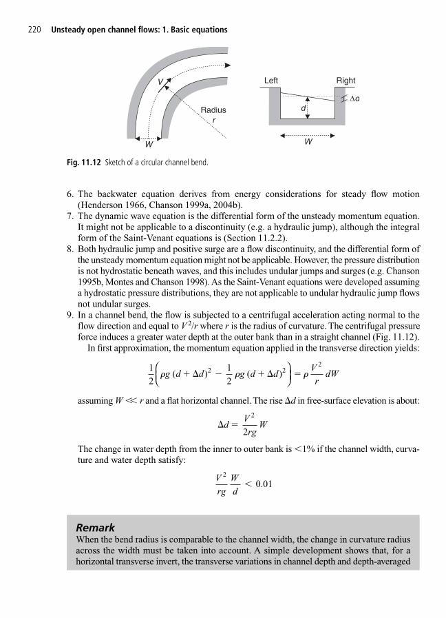
6. The backwater equation derives from energy considerations for steady flow motion(Henderson 1966, Chanson 1999a, 2004b).

7. The dynamic wave equation is the differential form of the unsteady momentum equation.It might not be applicable to a discontinuity (e.g. a hydraulic jump), although the integralform of the Saint-Venant equations is (Section 11.2.2).

8. Both hydraulic jump and positive surge are a flow discontinuity, and the differential form ofthe unsteady momentum equation might not be applicable. However, the pressure distributionis not hydrostatic beneath waves, and this includes undular jumps and surges (e.g. Chanson1995b, Montes and Chanson 1998). As the Saint-Venant equations were developed assuminga hydrostatic pressure distributions, they are not applicable to undular hydraulic jump flowsnot undular surges.

9. In a channel bend, the flow is subjected to a centrifugal acceleration acting normal to theflow direction and equal to V 2/r where r is the radius of curvature. The centrifugal pressureforce induces a greater water depth at the outer bank than in a straight channel (Fig. 11.12).

In first approximation, the momentum equation applied in the transverse direction yields:

assuming W �� r and a flat horizontal channel. The rise �d in free-surface elevation is about:

The change in water depth from the inner to outer bank is �1% if the channel width, curva-ture and water depth satisfy:

Vrg

Wd

2

0 01 � .

�dVrg

W �2

2

12

12

2 22

� � �g d d g d dVr

dW( ) ( ) � �� �

220 Unsteady open channel flows: 1. Basic equations

W

Radiusr

V

W

d

Left Right

∆d

Fig. 11.12 Sketch of a circular channel bend.

RemarkWhen the bend radius is comparable to the channel width, the change in curvature radiusacross the width must be taken into account. A simple development shows that, for ahorizontal transverse invert, the transverse variations in channel depth and depth-averaged

10.

where d is the water depth and W is the channel width.12. A small disturbance will propagate with a celerity C � �

__gd

__o. For a channel initially at

rest, the wave location, for an observer standing on the bank is given by the forwardcharacteristics trajectory:

Forward characteristics C1

The integration gives:

In a horizontal channel with the fluid initially at rest, So � 0 (horizontal channel) andSf � 0 (no flow). Along the forward characteristics, (V 2C) is a constant and it isequal to 7.7 m/s.

Note that, at the wave crest, the water depth is �do, hence the wave celerityis ��

__gd

__o. As a result, the velocity V becomes negative beneath the wave crest (Chapter

12, Section 12.2.1).13. Answer: x � 7.7 km, t � 120 s, V � 0.06 m/s, d � 2.34 m.

The flow conditions correspond to a reduction in flow rate. At x � 7.7 km andt � 120 s, q � 0.14 m2/s, compared to q1 � 0.77 m2/s and q2 � 0.71 m2/s at t � 0.

14. For a kinematic wave problem (i.e. So � Sf), the characteristic system of equations becomes:

Forward characteristics

Backward characteristicsDD

2 0f otV C g S S( ) ( )� � � � �

DD

2 0f otV C g S S( ) ( ) � � � �

x gd t o�

dd

0 oxt

V C gd� �

SQ

C d Wf

2

Chézy2 3 2

�

Sf

gd WQf 3 2

2 8

�

11.6 Exercise solutions 221

velocity satisfy respectively:

where r is the radial distance measured from the centre of curvature and V is the depth-averaged velocity (Henderson 1966, pp. 251–258). The results show that the waterdepth increases from the inner bank to the outer bank while the depth-averaged velocityis maximum at the inner bank. In practice, flow resistance affects the velocity field butmaximum velocity is observed towards the inner bank.

∂∂Vr

Vr

� �

∂∂dr

Vgr

2

�

along the characteristic trajectories:

Forward characteristics C1

Backward characteristics C2

At the intersection of the forward characteristics issuing from station 1 with the back-ward characteristics issuing from station 2, the trajectory equations satisfy:

where x and t are the location and time of the intersection. At the intersection, the flowproperties satisfy:

where C1 � �__gd

__1 and C2 � �

__gd

__2.

The solutions of the characteristic system of equations yields: x � 12.6 km, t � 263 s,V � 0.80 m/s, C � 2.44 m/s, d � 0.61 m and q � 0.49 m2/s. As a comparison,q1 � 0.325 m2/s and q2 � 0.30 m2/s at t � 0. That is, the flow situation corresponds to anincrease in flow rate.

18. At the latest (i.e. last) intersection of the characteristic curves, x � 1.61 km, t � 39 s,V � 0.59 m/s, C � 2.35 m/s. The flow conditions correspond to an increase in flowrate. At x � 1.61 km and t � 39 s, Q � 1.58 m3/s and d � 0.933 m, compared toQ1 � 1.45 m3/s and Q5 � 0.929 m3/s at t � 0.

19. At the latest (i.e. last) intersection of the characteristic curves, x � 421 m, t � 45 s,V � 0.59 m/s, C � 2.19 m/s.

The flow conditions correspond to a reduction in turbine discharge. At x � 421 m andt � 45 s, Q � 4.28 m3/s, compared to Q1 � 5.16 m3/s and Q5 � 5.15 m3/s at t � 0.

V C V C 2 2 2 � 2

V C V C 2 2 1 � 1

x x V C t ( )2 2 2� �

x x V C t ( )1 1 1�

dd

xt

V C� �

dd

xt

V C�

222 Unsteady open channel flows: 1. Basic equations

12

Unsteady open channel flows:2. Applications

SummaryIn this chapter the Saint-Venant equations for unsteady open channel flows areapplied. Basic applications include small waves and monoclinal waves, thesimple wave problem, positive and negative surges. The dam break wave istreated in Chapter 13.

12.1 Introduction

In unsteady open channel flows, the velocities and water depths change with time and longi-tudinal position. For one-dimensional applications, the continuity and momentum equationsyield the Saint-Venant equations (Chapter 11). The application of the Saint-Venant equationsis limited by some basic assumptions:

1. the flow is one-dimensional,2. the streamline curvature is very small and the pressure distributions are hydrostatic,3. the flow resistance are the same as for a steady uniform flow for the same depth and velocity,4. the bed slope is small enough to satisfy: cos � � 1 and sin � � tan � � �,5. the water density is a constant,6. the channel has fixed boundaries and sediment motion is neglected.

With these hypotheses, the unsteady flow can be characterized at any point and any time bytwo variables: e.g. V and Y where V is the flow velocity and Y is the free-surface elevation.The unsteady flow properties are described by a system of two partial differential equations:

(12.1)

(12.2)

where A is the cross-sectional area, B is the free-surface width, So is the bed slope and Sf isthe friction slope (Fig. 11.2). Equation (12.1) is the continuity equation and equation (12.2)is the dynamic equation.

∂∂

∂∂

∂∂

Vt

VVx

gYx

gS 0f �

∂∂

∂∂

∂∂

∂∂

Yt

AB

Vx

VYx

SVB

Ax

d

0oconstant

��

The Saint-Venant equations (12.1) and (12.2) cannot be solved analytically because of non-linear terms and of complicated functions. Examples of non-linear terms include thefriction slope Sf while complicated functions include the flow cross-section A(d) and free-surface width B(d) of natural channels. A mathematical technique to solve the system of partialdifferential equations formed by the Saint-Venant equations is the method of characteristics.It yields a characteristic system of equations:

Forward characteristic (12.3a)

Backward characteristic (12.3b)

along:

Forward characteristic C1 (12.4a)

Backward characteristic C2 (12.4b)

where C is celerity of a small disturbance for an observer travelling with the flow: C � ���gA/B�.For an observer travelling along the forward characteristic, equation (12.3a) is valid at any point.For an observer travelling in the backward characteristic, equation (12.3b) is satisfied every-where. The system of four equations formed by equations (12.3) and (12.4) represents the char-acteristic system of equations that replaces the differential form of the Saint-Venant equations.

12.2 Propagation of waves

12.2.1 Propagation of a small wave

Considering a simple wave propagating in a horizontal channel initially at rest, the waveheight is �d and the wave propagation speed (or celerity) is U (Fig. 12.1). For an observer

dd

xt

V C� �

dd

xt

V C�

DD

2 ) ( f otV C g S S( )� � � �

DD

2 ) ( f otV C g S S( ) � � �

224 Unsteady open channel flows: 2. Applications

RemarkAlong the forward characteristic trajectory:

the absolute derivative of (V 2C) equals:

Forward characteristic

Conversely, the absolute derivative of (V � 2C) along the backward characteristic is:

Backward characteristicDD

( 2 ) ( ) 2 )t

V Ct

V Cx

V C� � � �∂∂

∂∂

(

DD

( 2 ) ( ) 2 )t

V Ct

V Cx

V C � ∂∂

∂∂

(

dd

xt

V C�

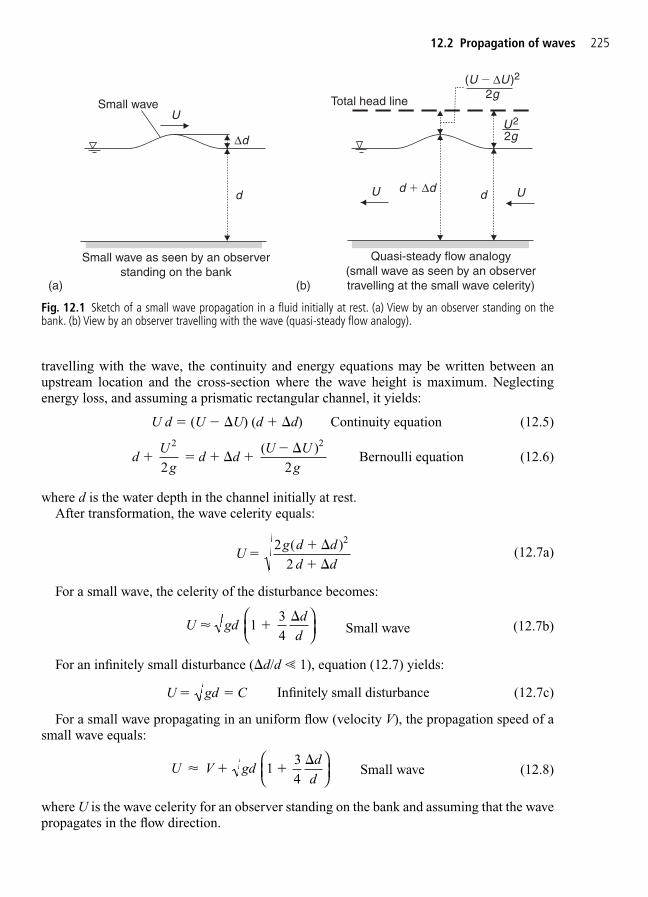
travelling with the wave, the continuity and energy equations may be written between anupstream location and the cross-section where the wave height is maximum. Neglectingenergy loss, and assuming a prismatic rectangular channel, it yields:

U d � (U � �U) (d �d) Continuity equation (12.5)

Bernoulli equation (12.6)

where d is the water depth in the channel initially at rest.After transformation, the wave celerity equals:

(12.7a)

For a small wave, the celerity of the disturbance becomes:

Small wave (12.7b)

For an infinitely small disturbance (�d/d # 1), equation (12.7) yields:

Infinitely small disturbance (12.7c)

For a small wave propagating in an uniform flow (velocity V), the propagation speed of asmall wave equals:

Small wave (12.8)

where U is the wave celerity for an observer standing on the bank and assuming that the wavepropagates in the flow direction.

U V gdd

d 1

34

� �

U gd C � �

U gdd

d� 1

34

�

Ug d d

d d

2 ( )

2

� �

�2

dU

gd d

U Ug

( )2 2

� �

2 2�

�

12.2 Propagation of waves 225

U Udd ∆d

Total head line

Quasi-steady flow analogy(small wave as seen by an observertravelling at the small wave celerity)

2gU2

2g(U � ∆U )2

USmall wave

Small wave as seen by an observerstanding on the bank

∆d

d

(a) (b)

Fig. 12.1 Sketch of a small wave propagation in a fluid initially at rest. (a) View by an observer standing on thebank. (b) View by an observer travelling with the wave (quasi-steady flow analogy).

12.2.2 Propagation of a known discharge (monoclinal wave)

Considering the propagation of a known flow rate Q2, the initial discharge is Q1 before thepassage of the monoclinal wave (Fig. 12.2). Upstream and downstream of the wave, the flowconditions are steady and the propagating wave is assumed to have a constant shape. Thecelerity of the wave must be greater than the downstream flow velocity. The continuity equationbetween sections 1 and 2 gives:

(U � V1) A1 � (U � V2) A2 (12.9)

where U is the wave celerity for an observer standing on the bank, V is the flow velocity, A isthe cross-sectional area, and the subscripts 1 and 2 refer to the initial and new steady flowconditions respectively. After transformation, it yields:

(12.10a)UQ QA A

2 1

2 1

��

�

226 Unsteady open channel flows: 2. Applications

A1A2

V1

V2Q2

U

2 1

Q1 � Q2

Fig. 12.2 Propagation of a monoclinal wave.

Notes1. A celerity is a characteristic velocity or speed. For example, the celerity of sound is

the sound speed.2. In July 1870, Barré de Saint-Venant derived equation (12.7) and he compared it

favourably with the experiments of H.E. Bazin (Barré de Saint-Venant 1871b, p. 239).3. Henri Emile Bazin (1829–1917) was a French hydraulician and engineer, member of

the French ‘Corps des Ponts-et-Chaussées’ and later of the Académie des Sciences deParis. He worked as an assistant of Henri P.G. Darcy at the beginning of his career.

4. Henri Philibert Gaspard Darcy (1805–1858) was a French civil engineer. He studiedat Ecole Polytechnique between 1821 and 1823, and later at the Ecole NationaleSupérieure des Ponts-et-Chaussées. He performed numerous experiments and he gavehis name to the Darcy–Weisbach friction factor and to the Darcy law in porous media.

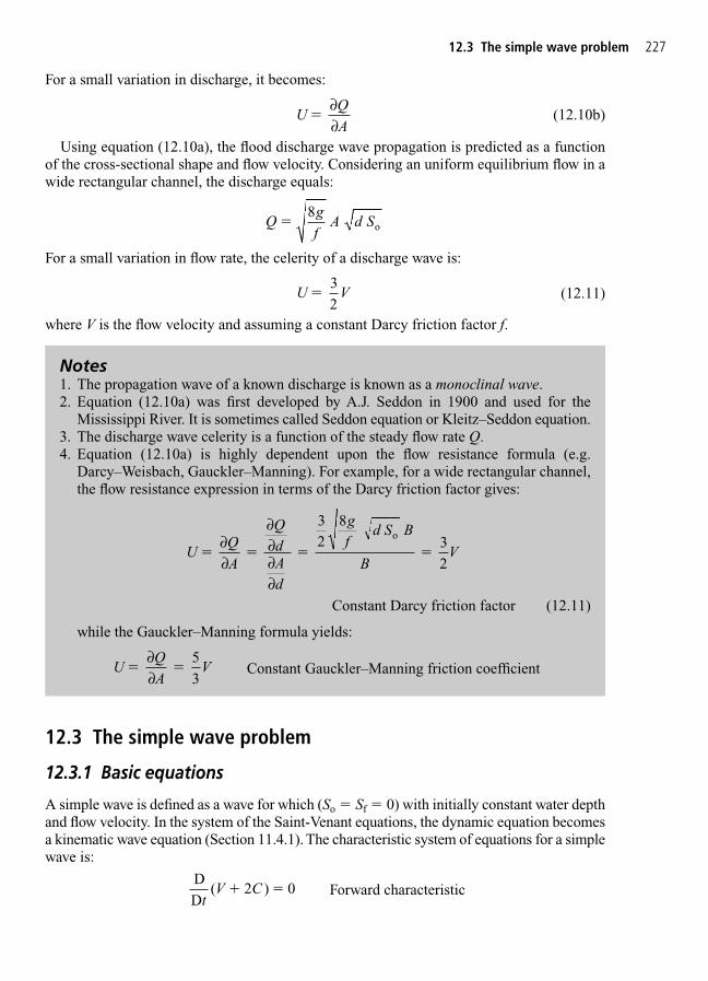
For a small variation in discharge, it becomes:

(12.10b)

Using equation (12.10a), the flood discharge wave propagation is predicted as a functionof the cross-sectional shape and flow velocity. Considering an uniform equilibrium flow in awide rectangular channel, the discharge equals:

For a small variation in flow rate, the celerity of a discharge wave is:

(12.11)

where V is the flow velocity and assuming a constant Darcy friction factor f.

12.3 The simple wave problem

12.3.1 Basic equations

A simple wave is defined as a wave for which (So � Sf � 0) with initially constant water depthand flow velocity. In the system of the Saint-Venant equations, the dynamic equation becomesa kinematic wave equation (Section 11.4.1). The characteristic system of equations for a simplewave is:

Forward characteristicDD

2 ) 0t

V C( �

U V 32

�

Qgf

A d S 8

o�

UQA

�∂∂

12.3 The simple wave problem 227

Notes1. The propagation wave of a known discharge is known as a monoclinal wave.2. Equation (12.10a) was first developed by A.J. Seddon in 1900 and used for the

Mississippi River. It is sometimes called Seddon equation or Kleitz–Seddon equation.3. The discharge wave celerity is a function of the steady flow rate Q.4. Equation (12.10a) is highly dependent upon the flow resistance formula (e.g.

Darcy–Weisbach, Gauckler–Manning). For example, for a wide rectangular channel,the flow resistance expression in terms of the Darcy friction factor gives:

Constant Darcy friction factor (12.11)

while the Gauckler–Manning formula yields:

Constant Gauckler–Manning friction coefficientUQA

V 53

� �∂∂

UQA

QdAd

gf

d S B

BV

32

32

o

� � � �∂∂

∂∂∂∂

8

Backward characteristicc

along:

Forward characteristic C1

Backward charcteristic C2

Basically (V 2C) is a constant along the forward characteristic. That is, for an observermoving at the absolute velocity (V C), the term (V 2C) is constant. Similarly (V � 2C)is constant along the backward characteristic. The characteristic trajectories can be plotted inthe (x, t) plane (Fig. 12.3). They represent the path of the observers travelling on the forwardand backward characteristics. On each forward characteristic, the slope of the trajectory is1/(V C) and (V 2C) is a constant along the characteristic trajectory. Altogether the char-acteristic trajectories form contour lines of (V 2C) and (V � 2C). For the simple waveproblem (So � Sf � 0), a family of characteristic trajectories is a series of straight lines if anyone curve of the family (i.e. C1 or C2) is a straight line (Henderson 1966).

In a simple wave problem, the initial flow conditions are uniform everywhere: i.e. V(x,t � 0) � Vo and d(x, t � 0) � do. At t � 0, a disturbance (i.e. a simple wave) is introduced,typically at the origin (x � 0, Fig. 12.3). The wave propagates to the right along the forwardcharacteristic C1 with a velocity (Vo Co) where Vo is the initial flow velocity and Co is theinitial celerity: Co � ��gAo/�Bo� (Fig. 12.3). If x � 0 is not a boundary condition, a similar rea-soning may be developed on the left side of the (x, t) plane following the negative character-istics issuing from the origin (e.g. Chapter 13). The disturbance must propagate into theundisturbed flow region with a celerity assumed to be Co implying that the wave front is assumedsmall enough. In the (x, t) plane, the positive characteristic D1–E2 divides the flow region

dd

xt

V C� �

dd

xt

V C�

DD

2 ) 0t

V C( � �

228 Unsteady open channel flows: 2. Applications

t

xD1

E1

Backwardcharacteristic

Forward characteristics

Initialforward

characteristic1

E2

F1

Zone of quiet(undisturbed flow)

Vo Co

Fig. 12.3 Characteristic curves of a simple wave.

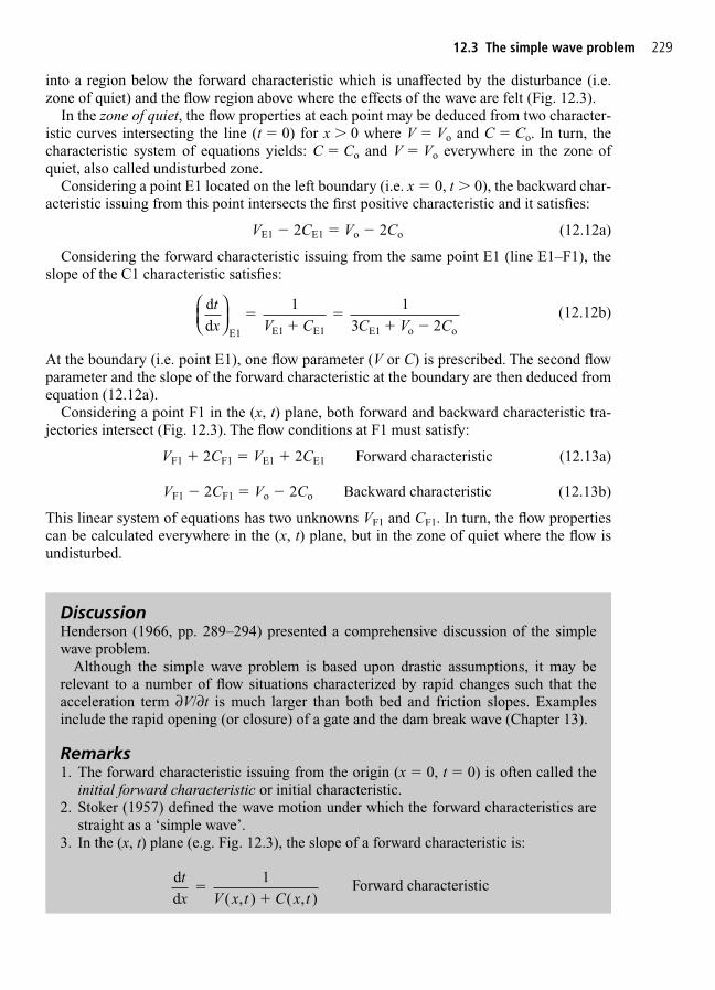
into a region below the forward characteristic which is unaffected by the disturbance (i.e.zone of quiet) and the flow region above where the effects of the wave are felt (Fig. 12.3).

In the zone of quiet, the flow properties at each point may be deduced from two character-istic curves intersecting the line (t � 0) for x � 0 where V � Vo and C � Co. In turn, thecharacteristic system of equations yields: C � Co and V � Vo everywhere in the zone ofquiet, also called undisturbed zone.

Considering a point E1 located on the left boundary (i.e. x � 0, t � 0), the backward char-acteristic issuing from this point intersects the first positive characteristic and it satisfies:

VE1 � 2CE1 � Vo � 2Co (12.12a)

Considering the forward characteristic issuing from the same point E1 (line E1–F1), theslope of the C1 characteristic satisfies:

(12.12b)

At the boundary (i.e. point E1), one flow parameter (V or C) is prescribed. The second flowparameter and the slope of the forward characteristic at the boundary are then deduced fromequation (12.12a).

Considering a point F1 in the (x, t) plane, both forward and backward characteristic tra-jectories intersect (Fig. 12.3). The flow conditions at F1 must satisfy:

VF1 2CF1 � VE1 2CE1 Forward characteristic (12.13a)

VF1 � 2CF1 � Vo � 2Co Backward characteristic (12.13b)

This linear system of equations has two unknowns VF1 and CF1. In turn, the flow propertiescan be calculated everywhere in the (x, t) plane, but in the zone of quiet where the flow isundisturbed.

dd

1

13 2

E1 E1 E1 E1 o o

tx V C C V C

�

� �

12.3 The simple wave problem 229

DiscussionHenderson (1966, pp. 289–294) presented a comprehensive discussion of the simplewave problem.

Although the simple wave problem is based upon drastic assumptions, it may be relevant to a number of flow situations characterized by rapid changes such that theacceleration term ∂V/∂t is much larger than both bed and friction slopes. Examplesinclude the rapid opening (or closure) of a gate and the dam break wave (Chapter 13).

Remarks1. The forward characteristic issuing from the origin (x � 0, t � 0) is often called the

initial forward characteristic or initial characteristic.2. Stoker (1957) defined the wave motion under which the forward characteristics are

straight as a ‘simple wave’.3. In the (x, t) plane (e.g. Fig. 12.3), the slope of a forward characteristic is:

Forward characteristicdd

1

( , ) ( , )tx V x t C x t

�

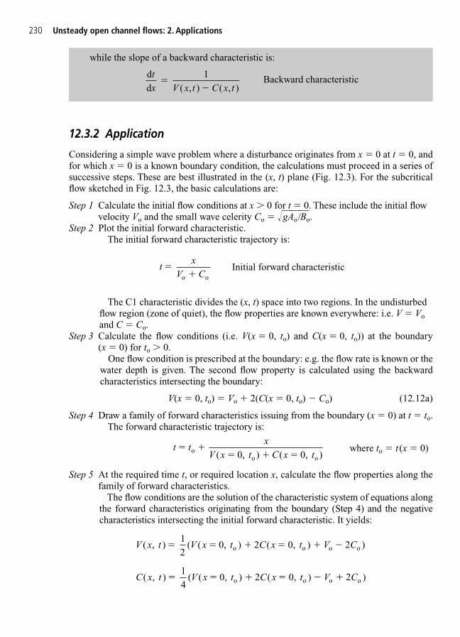
12.3.2 Application

Considering a simple wave problem where a disturbance originates from x � 0 at t � 0, andfor which x � 0 is a known boundary condition, the calculations must proceed in a series ofsuccessive steps. These are best illustrated in the (x, t) plane (Fig. 12.3). For the subcriticalflow sketched in Fig. 12.3, the basic calculations are:

Step 1 Calculate the initial flow conditions at x � 0 for t � 0. These include the initial flowvelocity Vo and the small wave celerity Co � ��gAo/�Bo�.

Step 2 Plot the initial forward characteristic.The initial forward characteristic trajectory is:

Initial forward characteristic

The C1 characteristic divides the (x, t) space into two regions. In the undisturbedflow region (zone of quiet), the flow properties are known everywhere: i.e. V � Voand C � Co.

Step 3 Calculate the flow conditions (i.e. V(x � 0, to) and C(x � 0, to)) at the boundary(x � 0) for to � 0.

One flow condition is prescribed at the boundary: e.g. the flow rate is known or the water depth is given. The second flow property is calculated using the backwardcharacteristics intersecting the boundary:

V(x � 0, to) � Vo 2(C(x � 0, to) � Co) (12.12a)

Step 4 Draw a family of forward characteristics issuing from the boundary (x � 0) at t � to.The forward characteristic trajectory is:

where to � t(x � 0)

Step 5 At the required time t, or required location x, calculate the flow properties along thefamily of forward characteristics.

The flow conditions are the solution of the characteristic system of equations along the forward characteristics originating from the boundary (Step 4) and the negative characteristics intersecting the initial forward characteristic. It yields:

C x t V x t C x t V C( , ) 14

( ( 0, 2 ( 2o o o o� � � � ) , ) )0

V x t V x t C x t V C( , ) 12

( ( 0, 2 ( 2o o o o� � � �) , ) )0

t tx

V x t C x t

( 0, ( 0, oo o

� � �) )

tx

V C

o o

�

230 Unsteady open channel flows: 2. Applications

while the slope of a backward characteristic is:

Backward characteristicdd

1

( , ) ( , )tx V x t C x t

��

DiscussionIt is important to remember the basic assumptions of the simple wave analysis. That is, awave for which So � Sf � 0 with initially constant water depth do and flow velocity Vo.Further the front of the wave is assumed small enough for the initial forward characteristictrajectory to satisfy dx/dt � Vo Co.

In the solution of the simple wave problem, Step 2 is important to assess the extent of theinfluence of the disturbance. In Steps 3 and 5, the celerity C is a function of the flow depth:C � ��gA�/B where the flow cross-section A and free-surface width B are both functions of thewater depth.

12.3 The simple wave problem 231

ApplicationA long irrigation channel is controlled by a downstream gate. During a gate operation,the flow velocity, immediately upstream of the gate, increases linearly from 0 to 1 m/s in2 min. Initially the flow is at rest and the water depth is 2 m. Neglecting bed slope andfriction slope, calculate the water depths at the gate, at mid-distance and at the canalintake for the next 10 min.

SolutionInitially the water in the canal is at rest and the water depth is 2 m everywhere.

The prescribed boundary condition at the downstream end is the velocity. Let select a coordinate system with x � 0 at the downstream end and x positive in the upstream direction.The initial conditions are Vo � 0 and Co � 4.43 m/s assuming a wide rectangular channel.

Then the flow conditions at the boundary (x � 0) are calculated at various times to:

C(x � 0, to) � 0.5(V(x � 0, to) � (Vo � 2Co)) (12.12a)

Next the C1 characteristic trajectories can be plotted from the left boundary (x � 0).As the initial C1 characteristic is a straight line, all the C1 characteristics are straightlines with the slope:

Results are shown in Fig. 12.4 for the first few minutes. Figure 12.4(a) presents three C1characteristics. Following the initial characteristic, the effects of the gate operation arefelt as far upstream as x � 1.59 km at t � 6 min.

At t � 6 min, the flow property between x � 0 and x � 1590 m are calculated from:

V(x, t � 6 min) 2C(x, t � 6 min) � V(x � 0, to) 2C(x � 0, to)

Forward characteristic

V(x, t � 6 min) � 2C(x, t � 6 min) � Vo � 2Co Backward characteristic

where the equation of the forward characteristic is:

Forward characteristict tx

V x t C x t

( 0, ( 0, oo o

� � �) )

dd

1

( , ) ( , )

1( 0, ( 0, o o

tx V x t C x t V x t C x t

�

�� �) )

d x tC x t

g( 0, )

( 0, )o

o� ��

232 Unsteady open channel flows: 2. Applications

These three equations are three unknowns: V(x, t � 6 min), C(x, t � 6 min) andto � t(x � 0) for the C1 characteristics. The results in terms of the water depth, flowvelocity and celerity at t � 6 min are presented in Fig. 12.4(b).

Remarks1. Practically, the calculations of the free-surface profile are best performed by selecting the

boundary point (i.e. the time to), calculating the flow properties at the boundary, and thendrawing the C1 characteristics until they intersect the horizontal line t � 6 min. That is,the computations follow the order; select to � t(x � 0), calculate d(x � 0, to), compute

0

100

200

300

400

500

600

0 200 400 600 800 1000 1200 1400 1600 1800 2000

C1 at t (x � 0) � 0C1 at t (x � 0) � 40 sC1 at t (x � 0) � 80 s

x (m)

t (s) Simple wave analysis

Zone of quiet (undisturbed flow)

(a)

�1

0

1

2

3

4

0 500 1000 1500 2000

Water depthVelocity VCelerity C

x (m)

Simple wave analysis

d (m), V (m/s), C (m/s)

(b)

Fig. 12.4 Simple wave solution. (a) Characteristic curves. (b) Free-surface profile at t � 6 min.

12.4 Positive and negative surges 233

V(x � 0, to), C(x � 0, to), plot the C1 characteristics, calculate x(t � 6 min) along the C1characteristics. Then compute V(x, t � 6 min) and C(x, t � 6 min):

Lastly the flow depth equals d � C2/g.2. In Fig. 12.4(b), note that the velocity is zero for x � 1.59 km at t � 6 min.3. Note that the C2 characteristics lines are not straight lines.4. A relevant example is Henderson (1966, pp. 192–294).

C x t V x t C x t V C, 6 min 0, 2 0, 2o o o o� � � � � ( ) ( ) ( )( )14

V x t V x t x t V C, 6 min 0, 2C 0, 2o o o o� � � � � ( ) ( ) ( )( )12

12.4 Positive and negative surges

12.4.1 Presentation

A surge (or wave) induced by a rise in water depth is called a positive surge. A negative surgeis associated with a reduction in water depth.

Considering a rise in water depth at the boundary, the increase in water depth induces anincrease in small wave celerity C with time because C � �g/d

–—for a rectangular channel. As

a result, the slope of the forward characteristics in the (x, t) plane decreases with increasingtime along the boundary (x � 0) as:

It follows that the series of forward characteristics issuing from the boundary conditionforms a network of converging lines (Fig. 12.5(a)).

Similarly, a negative surge is associated with a reduction in water depth, hence a decrease inwave celerity. The resulting forward characteristics issuing from the origin form a series ofdiverging straight lines (Fig. 12.5(b)). The negative wave is said to be dispersive. Locations ofconstant water depths move further apart as the wave moves outwards from the point of origin.

12.4.2 Positive surge

Although the positive surge may be analysed using a quasi-steady flow analogy (see below), itsinception and development is studied with the method of characteristics. When the water depthincreases with time, the forward characteristics converge and eventually intersect (Fig. 12.5(a),points E2, F2 and G2). The intersection of two forward characteristics implies that the water

dd

1

tx V C

�

Remarks1. A positive surge is also called bore, positive bore, moving hydraulic jump and posi-

tive wave. A positive surge of tidal origin is a tidal bore.2. A negative surge is sometimes called negative wave.

depth has two values at the same time. This anomaly corresponds to a wave front whichbecomes steeper and steeper until it forms an abrupt front: i.e. the positive surge front. Forexample, the forward characteristic issuing from E1 intersects the initial forward characteris-tic at E2 (Fig. 12.5(a)). For x � xE2, the equation of the initial forward characteristic (D1–E2)is no longer valid as indicated by the thin dashed line in Fig. 12.5(a).

After the formation of the positive surge, some energy loss takes place across the surge frontand the characteristic cannot be projected from one side of the positive surge to the other. Theforward characteristic E2–F2 becomes the ‘initial characteristic’ for xE2 � x � xF2. The points ofintersections (e.g. points E2, F2, G2) form an envelope defining the zone of quiet (Fig. 12.5(a)).

Practically, the positive surge forms at the first intersecting point: i.e. the intersection pointwith the smallest time t (Fig. 12.6). Figure 12.6 illustrates the development of a positive surgefrom the onset of the surge (i.e. first intersection of forward characteristics) until the surgereaches its final form. After the first intersection of forward characteristics, there is a waterdepth discontinuity along the forward characteristics forming the envelop of the surge front: e.g.between points E2 and F2, and F2 and G2 in Fig. 12.5. The flow conditions across the surgefront satisfy the continuity and momentum principles (see Discussion). Once fully developed,the surge front propagate as a stable bore (Figs 12.7 and 12.8).

234 Unsteady open channel flows: 2. Applications

1

t

xD1

Positive surge

Initial forward characteristic

1

E1

E2

F1

G1F2

G2

xs

ts

Envelope of the positivesurge front

Vo Co

V C

(a)

Zone of quiet(undisturbed flow)

t

xD1

Negative surge

Initial forward characteristic

Forwardcharacteristics

Zone of quiet(undisturbed flow)

1

Vo Co

1

V C

(b)

Fig. 12.5 Characteristic trajectories for (a) positive and (b) negative surges.

12.4 Positive and negative surges 235

t

x

Onset ofsurge front

Envelopeof surge front

Final form ofsurge front

1V C

1Vo Co

Per

iod

of in

crea

sing

(V

C) to

Fig. 12.6 Characteristic trajectories for the development of a positive surge.

(a-i) (a-ii)

(a-iii)

Fig. 12.7 Photographs of positive surges. (a) Advancing positive surge front in 0.5 m wide horizontal rectangularchannel – surge propagation from a-i to a-iii after complete gate closure: t � 1.5, 5 and 8.7 s after start gateclosure.

236 Unsteady open channel flows: 2. Applications

(b)

Fig. 12.7 (Contd) (b) Small tidal bore in the Baie du Mont Saint Michel (France), viewed from the Mont-Saint-Michelon 19 March 1996 (courtesy of Dr Pedro Lomonaco) – bore direction from right to left.

Quasi-steady flow analogyPositive surge as seen by an observer

travelling at the surge velocity

ddo

Vo U

V U

Positive surge(as seen by an observer standing

on the bank)Gate

closure U

VoV

ddo

Initial water level

Fig. 12.8 Quasi-steady flow analogy for a fully developed positive surge.

12.4 Positive and negative surges 237

Remarks1. A positive surge has often a breaking front. It may also consist of a train of free-

surface undulations if the surge Froude number is �1.35–1.4 (e.g. Chanson 1995b).Figure 12.7(a) show a breaking surge in a horizontal rectangular channel while Fig.12.7(b) illustrates a non-breaking undular surge in a natural channel.

2. Henderson (1966, pp. 294–304) presented a comprehensive treatment of the surgesusing the method of characteristics.

Discussion: fully developed positive surgeConsidering a fully developed positive surge in a rectangular channel (Fig. 12.8), thesurge is a unsteady flow situation for an observer standing on the bank. But the surge isseen by an observer travelling at the surge speed U as a steady flow called a quasi-steadyhydraulic jump.

For a smooth rectangular horizontal channel and considering a control volume acrossthe front of the surge (Fig. 12.8), the continuity and momentum equations become:

(Vo U)do � (V U) d Continuity equation

Momentum principle

where U is the surge velocity as seen by an observer immobile on the channel bank, thesubscript o refers to the initial flow conditions.

The continuity and momentum principles form a system of two equations with fivevariables (i.e. do, d, Vo, V, U). Usually the initial conditions Vo, do are known and thenew flow rate Q/Qo is determined by the rate of closure of the gate (e.g. complete closure: Q � 0, Fig. 12.7(a)).

The continuity and momentum equations yield:

where the surge Froude numbers Fro and Fr are defined as:

A positive surge travels faster than a small disturbance in front of it. The surge overtakesand absorbs any small disturbances that may exist at the free surface of the upstream

FrV U

gd

�

FrV U

gdo

o

o

�

FrFr

Fr

2

8 1

3/2o�

�1 12

3 2

/

dd

Fro

o2

12

1 8 1� �

� � �( ) ( 12

12o o o o

2 2V U d V V gd gd � � �)

Simple wave calculations of a positive surgeFor a simple wave, the apparition of the positive surge corresponds to the first intersectingpoint (point E2, Fig. 12.5(a)). The location and time of the wave front are deduced from thecharacteristic equation:

VE1 � 2CE1 � Vo � 2Co Backward characteristic to E1

and from the trajectory equations:

x � (Vo Co)t Initial forward characteristic

x � (VE1 CE1) (t � tE1) E1–E2 forward characteristic

where Vo and Co are the initial flow conditions. The first intersection of the two forward char-acteristics occurs at:

The reasoning may be extended to the intersection of two adjacent forward characteristics:e.g. the forward characteristics issuing from E1 and F1 and intersecting at F2, or the forwardcharacteristics issuing from F1 and G1 and intersecting at G2. It yields a more generalexpression of the surge location:

(12.14a)

(12.14b)

where C(x � 0, to) is the specified disturbance celerity at the origin and xs is the surge loca-tion at the time ts (Fig. 12.5(a)). If the specified disturbance is the flow rate Q(x � 0, to) or theflow velocity V(x � 0, to), equation (12.13b) may be substituted into equation (12.14).

Equation (12.14) is the equation of the envelope delimiting the zone of quiet and definingthe location of the positive surge front. The location where the surge first develops would cor-respond to point E2 in the (x, t) plane in Fig. 12.5(a).

t tx

V C x t Cs os

o o o

3 ( 0, ) 2

� � �

xV C x t C

C x tt

so o o

2

o

3 ( 0, ) 2

3( 0, )

� � �

�

( )∂

∂

tx

V CE2E2

o o

�

xV C V C C

C Ct

E2o o o E1 o

E1 o

E1

( ( 3 2

�

�

�

) )

3

238 Unsteady open channel flows: 2. Applications

water (i.e. in front of the surge). Similarly a positive surge travels more slowly thansmall disturbances behind it. Any small disturbance, downstream of the surge front andmoving upstream toward the wave front, overtakes the surge and is absorbed into it.Basically the wave absorbs random disturbances on both sides of the surge and thismakes the positive surge stable and self-perpetuating.

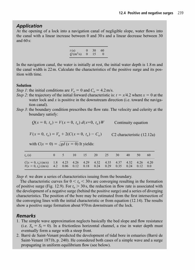
12.4 Positive and negative surges 239

ApplicationAt the opening of a lock into a navigation canal of negligible slope, water flows into the canal with a linear increase between 0 and 30 s and a linear decrease between 30 and 60 s:

t (s) 0 30 60Q (m3/s) 0 15 0

In the navigation canal, the water is initially at rest, the initial water depth is 1.8 m andthe canal width is 22 m. Calculate the characteristics of the positive surge and its pos-ition with time.

SolutionStep 1: the initial conditions are Vo � 0 and Co � 4.2 m/s.Step 2: the trajectory of the initial forward characteristic is: t � x/4.2 where x � 0 at the

water lock and x is positive in the downstream direction (i.e. toward the naviga-tion canal).

Step 3: the boundary condition prescribes the flow rate. The velocity and celerity at theboundary satisfy:

Continuity equation

C2 characteristic (12.12a)

with C(x � 0) � �gd——

(x � 0)——–

It yields:

Step 4: we draw a series of characteristics issuing from the boundary.The characteristic curves for 0 � to � 30 s are converging resulting in the formation

of positive surge (Fig. 12.9). For to � 30 s, the reduction in flow rate is associated withthe development of a negative surge (behind the positive surge) and a series of divergingcharacteristics. The position of the bore may be estimated from the first intersection ofthe converging lines with the initial characteristic or from equation (12.14). The resultsshow a positive surge formation about 970 m downstream of the lock.

Remarks1. The simple wave approximation neglects basically the bed slope and flow resistance

(i.e. So � Sf � 0). In a frictionless horizontal channel, a rise in water depth musteventually form a surge with a steep front.

2. Barré de Saint-Venant predicted the development of tidal bore in estuaries (Barré deSaint-Venant 1871b, p. 240). He considered both cases of a simple wave and a surgepropagating in uniform equilibrium flow (see below).

V x t V C x t C( 0, ) 2( ( 0, ) o o o o� � � � )

Q x t V x t d x t W( 0, ( 0, ( 0, )o o o� � � �) )

to (s) 0 5 10 15 20 25 30 40 50 60

C(x � 0, to) (m/s) 1.8 4.23 4.26 4.29 4.32 4.35 4.37 4.32 4.26 4.20V(x � 0, to) (m/s) 4.2 0.06 0.12 0.18 0.24 0.29 0.35 0.24 0.12 0.0

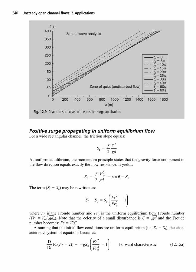
Positive surge propagating in uniform equilibrium flowFor a wide rectangular channel, the friction slope equals:

At uniform equilibrium, the momentum principle states that the gravity force component inthe flow direction equals exactly the flow resistance. It yields:

The term (Sf � So) may be rewritten as:

where Fr is the Froude number and Fro is the uniform equilibrium flow Froude number(Fro � Vo /��gdo). Note that the celerity of a small disturbance is C � ��gd and the Froudenumber becomes: Fr � V/C.

Assuming that the initial flow conditions are uniform equilibrium (i.e. So � Sf), the char-acteristic system of equations becomes:

Forward characteristic (12.15a)DD

( 2)) 1o

2

ot

C Fr gSFr

Fr( � � �

2

S S SFr

Frf o o

2

o2

1� � �

Sf V

gdSf

o2

oo

2 sin � � ��

Sf V

gdf

2

2

�

240 Unsteady open channel flows: 2. Applications

0

50

100

150

200

250

300

350

400

0 200 400 600 800 1000 1200 1400 1600 1800

to � 0to � 5 sto � 10 sto � 15 sto � 20 sto � 25 sto � 30 sto � 40 sto � 50 sto � 60 s

x (m)

t (s)

Simple wave analysis

Zone of quiet (undisturbed flow)

Fig. 12.9 Characteristic curves of the positive surge application.

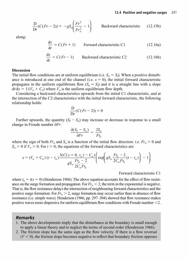
Backward characteristic (12.15b)

along:

Forward characteristic C1 (12.16a)

Backward characteristic C2 (12.16b)

DiscussionThe initial flow conditions are at uniform equilibrium (i.e. So � Sf). When a positive disturb-ance is introduced at one end of the channel (i.e. x � 0), the initial forward characteristicpropagates in the uniform equilibrium flow (So � Sf) and it is a straight line with a slopedt/dx � 1/(Vo Co) where Vo is the uniform equilibrium flow depth.

Considering a backward characteristics upwards from the initial C1 characteristic, and atthe intersection of the C2 characteristics with the initial forward characteristic, the followingrelationship holds:

Further upwards, the quantity (Sf � So) may increase or decrease in response to a smallchange in Froude number ∂Fr:

where the sign of both Fro and So is a function of the initial flow direction: i.e. Fro � 0 andSo � 0 if Vo � 0. For t � 0, the equations of the forward characteristics are:

Forward characteristic C1

where to � t(x � 0) (Henderson 1966). The above equation accounts for the effect of flow resist-ance on the surge formation and propagation. For Fro � 2, the term in the exponential is negative.That is, the flow resistance delays the intersection of neighbouring forward characteristics and thepositive surge formation. For Fro � 2, surge formation may occur earlier than in absence of flowresistance (i.e. simple wave). Henderson (1966, pp. 297–304) showed that flow resistance makespositive waves more dispersive for uniform equilibrium flow conditions with Froude number �2.

x V C t tC x t C

gSFrC Fr

gSFrC Fr

t t ( ( 3( ( 0,

2

2( 1o o o

o o

oo

o o

oo

o oo� �

� �

�

�� �) )

) )exp )

22

∂∂

( )S SFr

2SFr

f o o

o

��

DD

( 2)) 0t

C Fr( � �

dd

( 1)xt

C Fr� �

dd

( 1)xt

C Fr�

DD

( 2)) 1o

2

ot

C Fr gSFr

Fr( � � � �

2

12.4 Positive and negative surges 241

Remarks1. The above developments imply that the disturbance at the boundary is small enough

to apply a linear theory and to neglect the terms of second order (Henderson 1966).2. The friction slope has the same sign as the flow velocity. If there is a flow reversal

(V � 0), the friction slope becomes negative to reflect that boundary friction opposes

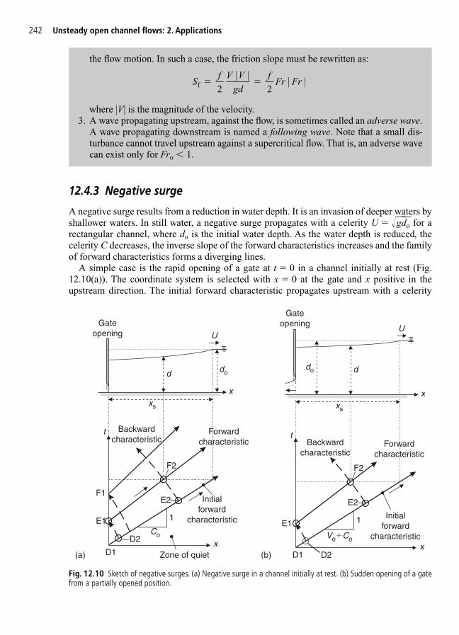
12.4.3 Negative surge

A negative surge results from a reduction in water depth. It is an invasion of deeper waters byshallower waters. In still water, a negative surge propagates with a celerity U � ��gd�o for arectangular channel, where do is the initial water depth. As the water depth is reduced, thecelerity C decreases, the inverse slope of the forward characteristics increases and the familyof forward characteristics forms a diverging lines.

A simple case is the rapid opening of a gate at t � 0 in a channel initially at rest (Fig.12.10(a)). The coordinate system is selected with x � 0 at the gate and x positive in theupstream direction. The initial forward characteristic propagates upstream with a celerity

242 Unsteady open channel flows: 2. Applications

the flow motion. In such a case, the friction slope must be rewritten as:

where |V| is the magnitude of the velocity.3. A wave propagating upstream, against the flow, is sometimes called an adverse wave.

A wave propagating downstream is named a following wave. Note that a small dis-turbance cannot travel upstream against a supercritical flow. That is, an adverse wavecan exist only for Fro � 1.

Sf V V

gdf

Fr Frf 2

2

| |� �| |

t

xD1

E1

D2

Backwardcharacteristic

Forwardcharacteristic

Initialforward

characteristic

E2

F2

F1

Zone of quiet

1

Co

x

U

Gateopening

do

xs

d

(a)

Backwardcharacteristic

Forwardcharacteristic

Initialforward

characteristic

t

xD1 D2

E1

E2

F2

1

VoCo

Gateopening

do

x

U

xs

d

(b)

Fig. 12.10 Sketch of negative surges. (a) Negative surge in a channel initially at rest. (b) Sudden opening of a gatefrom a partially opened position.

U � ��gd�o where do is the initial water depth. The location of the leading edge of the nega-tive surge is:

Note that the gate opening induces a negative flow velocity.A backward characteristic can be drawn issuing from the initial forward characteristic for

t � 0 (e.g. point D2) and intersecting the boundary conditions at the gate (e.g. point E1). Thebackward characteristic satisfies:

V(x � 0, to) � 2C(x � 0, to) � �2Co (12.17)

At the intersection of a forward characteristic issuing from the gate (e.g. at point E1) witha backwater characteristic issuing from the initial forward characteristic, the following con-ditions are satisfied:

VF2 2CF2 � V(x � 0, to) 2C(x � 0, to) (12.18)

VF2 � 2CF2 � �2Co (12.19)

where the point F2 is sketched in Fig. 12.10(a). Equations (12.17)–(12.18), plus the pre-scribed boundary condition, form a system of four equations with four unknowns VF2, CF2,V(x � 0, to) and C(x � 0, to). (In Fig. 12.10(a), VE1 � V(x � 0, to) and CE2 � C(x � 0, to).)In turn all the flow properties at the point F2 can be calculated.

In the particular case of a simple wave (paragraph 12.3), the forward characteristics arestraight lines because the initial forward characteristic is a straight line (paragraph 12.3.1).The equation of forward characteristics issuing from the gate (e.g. from point E1) is:

Simple wave approximation

The integration gives the water surface profile between the leading edge of the negativewave and the wave front:

for 0 " x " xs (12.20)

assuming a rectangular channel. At a given time t � to, the free-surface profile (equation(12.20)) is a parabola.

The gate opening corresponds to an increase of flow rate beneath the gate. It is associatedwith both the propagation of a negative surge upstream of the gate and the propagation of thepositive surge downstream of the gate.

xt t

gd gd

3 2o

o�

� �

dd

( 0, ( 0, 3 2o o oxt

V x t C x t V C C C� � � � � �) )

x gd ts o �

12.4 Positive and negative surges 243

Remarks1. A negative surge is associated with a gradual decrease in water depth and the surge

front is hardly discernible because the free-surface curvature is very shallow.2. In the above application, the gate is partially opened from an initially closed position:

i.e. Vo � 0.3. In a particular case, experimental observations showed that the celerity of the negative

surge was greater than the ideal value U � ���gdo (see Chapter 13). The differencewas thought to be caused by streamline curvature effects at the leading edge of thenegative surge.

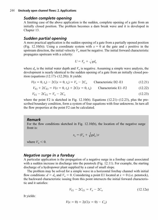
Sudden complete openingA limiting case of the above application is the sudden, complete opening of a gate from aninitially closed position. The problem becomes a dam break wave and it is developed inChapter 13.

Sudden partial openingA more practical application is the sudden opening of a gate from a partially opened position(Fig. 12.10(b)). Using a coordinate system with x � 0 at the gate and x positive in theupstream direction, the initial velocity Vo must be negative. The initial forward characteristicpropagates upstream with a celerity:

where do is the initial water depth and Vo is negative. Assuming a simple wave analysis, thedevelopment is nearly identical to the sudden opening of a gate from an initially closed pos-ition (equations (12.17)–(12.20)). It yields:

V(x � 0, to) � 2C(x � 0, to) � Vo � 2Co Characteristic D2–E1 (12.21)

VF2 2CF2 � V(x � 0, to) 2C(x � 0, to) Characteristic E1–F2 (12.22)

VF2 � 2CF2 � Vo � 2Co (12.23)

where the point F2 is sketched in Fig. 12.10(b). Equations (12.21)–(12.23), plus the pre-scribed boundary condition, form a system of four equations with four unknowns. In turn allthe flow properties at the point F2 can be calculated.

Negative surge in a forebayA particular application is the propagation of a negative surge in a forebay canal associatedwith a sudden increase in discharge into the penstock (Fig. 12.11). For example, the startingdischarge of a hydropower plant supplied by a canal of small slope.

The problem may be solved for a simple wave in a horizontal forebay channel with initialflow conditions: d � do and Vo � 0. Considering a point E1 located at x � 0 (i.e. penstock),the backward characteristic issuing from this point intersects the initial forward characteris-tic and it satisfies:

VE1 � 2CE1 � Vo � 2Co (12.12a)

It yields:

V(x � 0) � 2(C(x � 0) � Co)

U V gd o o�

244 Unsteady open channel flows: 2. Applications

RemarkFor the flow conditions sketched in Fig. 12.10(b), the location of the negative surge front is:

where Vo � 0.

x V gd ts o o ( � )

12.4 Positive and negative surges 245

(a-i)

(a-ii)

Fig. 12.11 Forebay canal. (a) Photographs of the forebay canal upstream of the inverted siphon on the Toyohashi-Tahara aqueduct (Japan) on 23 January 1999. The siphon characteristics are: length � 2780 m, diameter � 3.1 m,design flow � 17.1 m3/s. (a-i) Main canal immediately upstream the gates. (a-ii) Gates controlling the flow into theinverted siphon.

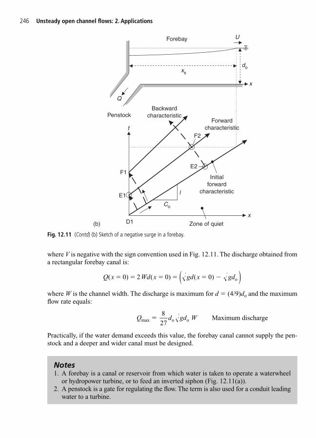
where V is negative with the sign convention used in Fig. 12.11. The discharge obtained froma rectangular forebay canal is:

where W is the channel width. The discharge is maximum for d � (4/9)do and the maximumflow rate equals:

Maximum discharge

Practically, if the water demand exceeds this value, the forebay canal cannot supply the pen-stock and a deeper and wider canal must be designed.

Q d gd Wmax o o 827

�

Q x Wd x gd x gd( 0) 2 ( 0) ( 0) o� � � � � �( )

246 Unsteady open channel flows: 2. Applications

t

xD1

E1

Backwardcharacteristic

Forwardcharacteristic

Initialforward

characteristic

F1E2

F2

Zone of quiet

l

Co

x

U

doxs

Q

Penstock

Forebay

(b)

Fig. 12.11 (Contd) (b) Sketch of a negative surge in a forebay.

Notes1. A forebay is a canal or reservoir from which water is taken to operate a waterwheel

or hydropower turbine, or to feed an inverted siphon (Fig. 12.11(a)).2. A penstock is a gate for regulating the flow. The term is also used for a conduit leading

water to a turbine.

12.5 The kinematic wave problem

12.5.1 Presentation

In a kinematic wave model, the differential form of the Saint-Venant equations is written as:

Continuity equation (12.24)

Sf � So � 0 Kinematic wave equation (12.25)

That is, the dynamic wave equation is simplified by neglecting the acceleration and inertialterms, and the free surface is assumed parallel to the channel bottom (paragraph 11.4.1,Chapter 11). The kinematic wave equation may be rewritten as:

where Q is the total discharge in the cross-section, f is the Darcy friction factor, A is the flowcross-sectional area and DH is the hydraulic diameter. Equation (12.25) expresses an uniquerelationship between the flow rate Q and the water depth d, hence the cross-sectional area at agiven location x. The differentiation of the flow rate with respect of time may be transformed:

The continuity equation becomes:

Continuity equation (12.26)

It may be rewritten as:

(12.27)

along:

(12.28)dd

=constant

xt

QA

x

�∂∂

DD

dd

0Qt

Qt

xt

Qx

� �∂∂

∂∂

∂∂

∂∂

∂∂

Qt

QA

Qx

x

0constant

��

∂∂

∂∂

∂∂

Qt

QA

At

x

constant

��

Qgf

AD

S 8

Ho�

4

∂∂

∂∂

At

Qx

0 �

12.5 The kinematic wave problem 247

3. The maximum flow rate for the simple wave approximation corresponds toQ2/(gW 2d3) � 1. That is, critical flow conditions. The flow rate equals the dischargeat the dam break site for a dam break wave in an initially dry, horizontal channel bed(Chapter 13).

4. The operation of penstocks and inverted siphon systems is associated with both sudden water demand and stoppage. The latter creates a positive surge propagatingupstream in the forebay channel (e.g. Fig. 12.11(a)).

That is, the discharge is constant along the characteristic trajectory defined by equation(12.28).

12.5.2 Discussion

The trajectories defined by equation (12.28) are the characteristics of equations (12.26) and(12.27). There is only one family of characteristics which all propagate in the same direction:i.e. in the flow direction (Fig. 12.12). The solution of the continuity equation in terms of theflow rate Q(x, t), in a river reach (x1 " x " x2) and for t � 0, requires one prescribed initialcondition at t � 0 and x1 " x " x2, and one prescribed upstream condition (x � x1) for t � 0.No prescribed downstream condition is necessary.

The kinematic wave model can only describe the downstream propagation of a disturb-ance. In comparison, the dynamic waves can propagate both upstream and downstream.Practically the kinematic wave equation is used to describe the translation of flood waves in some simple cases. One example is the monoclinal wave (paragraph 12.2.2). But the kinematic wave routing cannot predict the subsidence of flood wave and it has therefore limited applications.

248 Unsteady open channel flows: 2. Applications

Note1. The term

is sometimes called the speed of the kinematic wave.

dd

constant

xt

QA

x

��

∂∂

t

D3D2

E1

E2

x1 x2

Characteristics

xD1

Fig. 12.12 Characteristics of the kinematic wave problem.

12.6 The diffusion wave problem

12.6.1 Presentation

The diffusion wave equation is a simplification of the dynamic equation assuming that theacceleration and inertial terms are negligible. The differential form of the Saint-Venant equa-tions becomes:

Continuity equation (12.29a)

Diffusion wave equation (12.29b)

The definition of the friction slope gives:

(12.30)

where |Q| is the magnitude of the flow rate.Assuming a constant free-surface width B, the continuity equation (12.29a) is differenti-

ated with respect to x, and the diffusion wave equation (12.29b) is differentiated with respectof the time t. It yields:

(12.31a)

(12.31b)

The latter equation becomes:

(12.31c)

Noting that:

∂∂

∂∂

∂∂

∂∂

∂∂

t

Agf

Dd

Agf

D dt d

Agf

DB

Qx

8

8

8 H H H

4 4 41

� � �

∂∂ ∂

∂∂

∂∂

2

3 2

4 4

4d

t xQ

gf

AD

Qt

Q Q

gf

AD t

Agf

D

2 | |8

2 | |

8

8 0

2 H 2 H

H � �/

∂∂ ∂

∂∂

2dt x t

S S 0f o � �( )

Bd

x tQ

x

∂∂ ∂

∂∂

2

2 0 �

2

SQ Q

gf

ADf

2 H

| |8

�

4

∂∂dx

S S 0f o � �

Bdt

Qx

∂∂

∂∂

0 �

12.6 The diffusion wave problem 249

Notes1. The subsidence of the flood wave is the trend to flatten out the flood peak discharge.2. In summary, a kinematic wave model may predict the translation of a flood wave but

not its subsidence (i.e. flattening out). The latter may be predicted with the diffusionwave model (paragraph 12.6).

3. An application of the kinematic wave equation will be developed for a dam breakwave down sloping channel (Chapter 13).

and by eliminating (∂2d/∂x ∂t) between equations (12.31a) and (12.31c), the diffusive waveequation becomes:

(12.32a)

This equation may be rewritten as:

(12.32b)

Equation (12.32b) is an advective diffusion equation in terms of the discharge:

(12.32c)

where U and Dt are respectively the celerity of the diffusion wave and the diffusion coeffi-cient (Chapters 6 and 7). The advection velocity and diffusion coefficient are defined as:

Considering a limited river reach (x1 " x " x2), the solution of the diffusion wave equationin terms of the flow rate Q(x, t) requires the prescribed initial condition Q(x, 0) for t � 0 andx1 " x " x2, and one prescribed condition at each boundary (i.e. Q(x1, t) and Q(x2, t)) for t � 0.

Once the diffusion wave equation (12.32c) is solved in terms of the flow rates, the waterdepths are calculated from the continuity equation:

Continuity equation (12.29a)Bdt

Qx

∂∂

∂∂

0 �

D

gf

AD

B Qt

2 H

8

| |�

42

UQ

Bgf

AD d

Agf

D

8

8

2 H

H�

4

4∂

∂

∂∂

∂∂

∂∂

Qt

UQt

DQ

x t 2 �

2

∂∂

∂∂

∂∂

∂∂

Qt

Q

Bgf

AD d

Agf

D Qx

gf

AD

B QQ

x

8

8

8

| |2 H

H

2 H

2 �

4

44

2

2

�

�

1

2 | |8

2 | |

8

8

0

22 H

2 H

H

BQ

x

Qgf

AD

Qt

Q Q

Bgf

AD d

Agf

D Qx

∂∂

∂∂

∂∂

∂∂

2

3 2

4

4

4/

250 Unsteady open channel flows: 2. Applications

Notes1. The diffusion wave problem is also called diffusion routing.2. The term ‘routing’ or ‘flow routing’ refers to the tracking in space and time of a

flood wave.

ApplicationFor a rectangular channel and assuming a constant Darcy friction factor, the following rela-tionship holds:

Rectangular channel

The speed of the diffusion wave equals:

For a wide rectangular channel, the friction slope equals:

Assuming a constant Darcy friction factor f, the following relationship holds:

Hence, for a wide rectangular channel and assuming a constant Darcy friction factor, thecelerity of the diffusion wave equals:

The celerity of the wave is equal to the celerity of the monoclinal wave. But the diffusionwave flattens out with longitudinal distance while the monoclinal wave has a constant shape(paragraph 12.2.2).

12.6.2 Discussion

For constant diffusion wave celerity U and diffusion coefficient Dt, equation (12.32c) may besolved analytically for a number of basic boundary conditions. Further, since equation (12.32c)is linear, the theory of superposition may be used to build-up solutions with more complexproblems and boundary conditions (Chapters 5 and 6). Mathematical solutions of the

U V 32

�

∂∂

d

Agf

DB

gf

dQ

S d

8

32

8

32

H

f4

� �

SQ Qgf

B df

2 3

| |�

8

U VA

BP

32

1 23 w

� �

∂∂

dA

gf

DB

gf

AP

ABP

Q

S d

ABP

8

32

8 1

23

32

1 23

H

w w

f w

4� �

� �

12.6 The diffusion wave problem 251

3. The above development was performed assuming a constant free-surface width B.4. The diffusion coefficient may be rewritten as:

DQBSt

f

2

�

diffusion and heat equations were addressed in two classical references (Crank 1956,Carslaw and Jaeger 1959). Simple analytical solutions of the diffusion wave equation aresummarized in Table 12.1 assuming constant diffusion wave speed and diffusion coefficient.The flow situations are sketched in Fig. 12.13.

252 Unsteady open channel flows: 2. Applications

Table 12.1 Analytical solutions of the diffusion wave equation assuming constant diffusion wave celerity and diffusion coefficient

Problem Analytical solution Initial/boundary conditions(1) (2) (3)

Advective diffusion Q(x, 0) � Qo for x � 0 of a sharp front Q(x, 0) � Qo Q for x � 0

Initial volume slug introduced Q(x, 0) � Qo for t � 0at t � 0 and x � 0 Sudden injection of a water (i.e. sudden volume injection) discharge (Vol) at a rate

Q at origin at t � 0

Sudden discharge injection Q(0, t) � Qo Qin a river at a steady rate for 0 � t � �

Q(x, 0) � Qofor 0 � x � �

Note: erf � Gaussian error function (Appendix A, Section 12.7).

Q x t QQ

A D t

x Ut

D t( , )

Vol

4exp

) o

t

2

t� �

�

�

(

4

Q x t QQ x Ut

D t( , )

2 1 erf

4o

t

� ��

Q x t QQ x Ut

D t

Ux

D

x Ut

D t

( , ) 2

1 erf

4

exp 1 erf

4

ot

t t

� ��

�

x

Advective diffusiondownstream ofslug injection

Q

U

x

Advective diffusionof a sharp front

UQ

Q(x � 0,t � 0) � Qo

Q(x � 0, t � 0) � Qo �Q

x

Sudden steadydischarge injection

at origin

Q

Q(x � 0,t � 0) � Qo

Q(x � 0, t � 0) � Qo �Q

Fig. 12.13 Basic examples of advective diffusion problems.

Note some basic limitations of such analytical solutions. First the diffusion coefficient Dtis a function of the flow rate. It may be assumed constant only if the change in discharge issmall. Second the diffusion wave celerity is a function of the flow velocity and hence of theflow conditions.

12.6.3 The Cunge–Muskingum method

A simplification of the diffusion wave model is the Cunge–Muskingum method which wasdeveloped as an extension of the empirical Muskingum method.

Empiricism: the Muskingum method!?The Muskingum method is based upon the continuity equation for a river reach(x1 " x " x2):

Continuity equation

where Vol is the reach volume, Q1 � Q(x � x1) is the inflow and Q2 � Q(x � x2) is the out-flow. The method assumes a relationship between the reach volume, and the inflow and out-flow rates:

Vol � KM(XMQ1 (1 � XM) Q2)

where KM and XM are empirical routing parameters of the river reach. By differentiating theabove equation with respect to time and replacing into the continuity equation, it yields:

assuming constant routing parameters KM and XM. If the inflow rate is a known function oftime, the equation may be solved analytically or numerically in terms of the outflow Q2.

Developed in the 1930s for flood control schemes in the Muskingum River catchment (USA),the Muskingum method is a purely empirical, intuitive method: ‘the method uses the con-tinuity equation together with an empirical relation linking the stored volume to the dis-charge’ (Montes 1998, p. 572); ‘despite the popularity of the basic method, it cannot beclaimed that it is logically complete’ (Henderson 1966, p. 364); ‘although the conventionalflood-routing methods [including Muskingum] may give good results under some conditions,they have the tendency to be treacherous and unreliable’ (Thomas in Miller and Cunge 1975,p. 246). Cunge et al. (1980) further stressed: if ‘a forecasting system using the Muskingummethod was built for a river basin and then a series of hydraulic works changed the river’s flowcharacteristics, the forecasting system might well become useless and it might be necessary towait 20 years in order to have enough new calibration data’ (Cunge et al. 1980, p. 355).

Q K XQt

Q K XQt2 M M

21 M M

1 (1 dd

dd

� � �)

dVold

( 2 1tQ Q� � � )

12.6 The diffusion wave problem 253

DiscussionThe Muskingum method may be applied to specific situations to solve the downstreamflow conditions as functions of the upstream flow conditions. Note that the downstreamflow conditions have no influence on the upstream conditions, and the parameters KM

Cunge–Muskingum methodThe above method approaches a diffusion wave problem when:

where (x2 � x1) is the river reach length, and KM and XM are the Muskingum routing param-eters of the river reach. In turn, the routing parameters become functions of the flow rate:

This technique is called the Cunge–Muskingum method.

Kx x

Q

Bgf

AD d

Agf

DM

2 1

H

H

8

��

21 2

4

84

∂∂

/

X

Agf

D

x x Q Qd

Agf

DM

H

2 1H

12

8

| |8

� �

�

14

4

3

∂∂

( )

D X U x xt M 2 1 ( � � �12

)

Ux x

K

2 1

M

��

254 Unsteady open channel flows: 2. Applications

and XM must be calibrated and validated for each reach. The routing parameters are cal-culated from the inflow and outflow hydrographs of past floods in the reach.

Notes1. The parameters KM and XM are completely empirical: i.e. they have not theoretical

justification. The routing parameter KM is homogeneous to a time while the param-eter XM is dimensionless between 0 and 1.

2. XM must be between 0 and 0.5 for the method to be stable. For XM � 0.5, the floodpeak increases with distance.

3. For XM � 0, the Muskingum method becomes a simple reservoir storage problem.For XM � 0.5, the flood motion is a pure translation without attenuation and theMuskingum method approaches the kinematic wave solution.

DiscussionThe Cunge–Muskingum method may be applied to specific situations to solve the down-stream flow conditions as functions of the upstream flow conditions. Limitationsinclude: (1) the inertial terms must be negligible, (2) the downstream flow conditionshave no influence on the upstream conditions and (3) the parameters KM and XM must becalibrated and validated for the reach.

12.7 Appendix A – Gaussian error functions

12.7.1 Gaussian error function

The Gaussian error function erf is defined as:

(12A.1)

Values of the Gaussian error function are summarized in Table 12A.1. Basic properties of thefunction are:

erf(0) � 0 (12A.2)

erf(�) � 1 (12A.3)

erf(�u) � �erf(u) (12A.4)

(12A.5)

(12A.6)

where n! � 1 � 2 � 3 � … � n.

erf( ) 1 exp( )

1

1

2

1 3

(2

1 3 5

(2

2

2 2 2u

u

u u u u� �

��

�

�

��

� �

�

� ) )2 3K

erf( ) 1

!

2!

3!

3 5 7

u uu u u

� ��

�

��

� 3 1 5 7

L

erf( ) 2

duu

� ��

�exp( )�2

0∫

12.7 Appendix A – Gaussian error functions 255

In the Cunge–Muskingum method, the routing parameters KM and XM may be calculatedfrom the physical characteristics of the channel reach, rather than on previous floodrecords only.

Notes1. The extension of the Muskingum method was first presented by Cunge (1969).2. Jean A. Cunge worked in France at Sogreah in Grenoble and he lectured at the

Hydraulics and Mechanical Engineering School of Grenoble (ENSHMG).

Table 12A.1 Values of the error function erf

u erf(u) u erf(u)

0 0 1 0.84270.1 0.1129 1.2 0.91030.2 0.2227 1.4 0.95230.3 0.3286 1.6 0.97630.4 0.4284 1.8 0.98910.5 0.5205 2 0.99530.6 0.6309 2.5 0.99960.7 0.6778 3 0.999980.8 0.7421 � 10.9 0.7969

12.7.2 Complementary error function

The complementary Gaussian error function erfc is defined as:

(12A.7)

Basic properties of the complementary function include:

erfc(0) � 1 (12A.8)

erf(�) � 0 (12A.9)

12.8 Exercises

1. List the key assumptions of the Saint-Venant equations.2. What is the celerity of a small disturbance in (1) a rectangular channel, (2) a 90° V-shaped

channel and (3) a channel of irregular cross-section? (4) Application: a flow cross-sectionof a flood plain has the following properties: hydraulic diameter � 5.14 m, maximum waterdepth � 2.9 m, wetted perimeter � 35 m, free-surface width � 30 m. Calculate the celer-ity of a small disturbance.

3. A 0.2 m high small wave propagates downstream in a horizontal channel with initial flowconditions V � 0.1 m/s and d � 2.2 m. Calculate the propagation speed of the small wave.

4. Uniform equilibrium flow conditions are achieved in a long rectangular channel(W � 12.8 m, concrete lined, So � 0.0005). The observed water depth is 1.75 m. Calculatethe celerity of a small monoclinal wave propagating downstream. Perform your calcula-tions using the Darcy friction factor.

5. The flow rate in a rectangular canal (W � 3.4 m, concrete lined, So � 0.0007) is 3.1 m3/sand uniform equilibrium flow conditions are achieved. The discharge suddenly increases

erfc( ) 1 erf( ) 2

exp( d2u uu

� � � �

��� )

∞

∫

256 Unsteady open channel flows: 2. Applications

NotesIn first approximation, the function erf(u) may be correlated by:

erf(u) � u (1.375511 � 0.61044u 0.088439u2) 0 " u � 2

erf(u) � tanh(1.198787u) �� � u � �

In many applications, the above correlations are not accurate enough, and equation(12A.5) and Table 12A.1 should be used.

For small values of u, the error function is about:

Small values of u

For large values of u, the erf function is about:

Large values of uerf( ) 1 exp(

2

uu

u� �

� )

�

erf( ) uu

��

to 5.9 m3/s. Calculate the celerity of the monoclinal wave. How long will it take for themonoclinal wave to travel 20 km?

6. What is the basic definition of a simple wave? May the simple wave theory be applied to(1) a sloping, frictionless channel, (2) a horizontal, rough canal, (3) a positive surge in ahorizontal, smooth channel with constant water depth and (4) a smooth, horizontal canalwith an initially accelerating flow?

7. What is the ‘zone of quiet’?8. Another basic application is a river discharging into the sea and the upstream extent of

tidal influence onto the free surface. Considering a stream discharging into the sea, thetidal range is 0.8 m and the tidal period is 12 h 25 min. The initial flow conditions areV � 0.3 m/s, d � 0.4 m corresponding to low tide. Neglecting bed slope and flow resist-ance, and starting at a low tide, calculate how far upstream the river level will rise 3 hafter low tide and predict the free-surface profile at t � 3 h.

9. Considering a long, horizontal rectangular channel (W � 4.2 m), a gate operation, at oneend of the canal, induces a sudden withdrawal of water resulting in a negative velocity.At the gate, the boundary conditions for t � 0 are: V(x � 0, t) � �0.2 m/s. Calculate theextent of the gate operation influence in the canal at t � 1 h. The initial conditions in thecanal are: V � 0 and d � 1.4 m.

10. Water flows in an irrigation canal at steady state (V � 0.9 m/s, d � 1.65 m). The flume isassumed smooth and horizontal. The flow is controlled by a downstream gate. At t � 0,the gate is very slowly raised and the water depth upstream of the gate decreases at a rateof 5 cm/min until the water depth becomes 0.85 m. (1) Plot the free-surface profile att � 10 min. (2) Calculate the discharge per unit width at the gate at t � 10 min.

11. A 200 km long rectangular channel (W � 3.2 m) has a reservoir at the upstream end and agate at the downstream end. Initially the flow conditions in the canal are uniform:V � 0.35 m/s, d � 1.05 m. The water surface level in the reservoir begins to rise at a rate of0.2 m/h for 6 h. Calculate the flow conditions in the canal at t � 2 h. Assume So � Sf � 0.

12. Waters flow in a horizontal, smooth rectangular channel. The initial flow conditions ared � 2.1 m and V � 0.3 m/s. The flow rate is stopped by sudden gate closure at thedownstream end of the canal. Using the quasi-steady flow analogy, calculate the newwater depth and the speed of the fully developed surge front.

13. Let consider the same problem as above (i.e. a horizontal, smooth rectangular channel,d � 2.1 m and V � 0.3 m/s) but the downstream gate is closed slowly at a rate corres-ponding to a linear decrease in flow rate from 0.63 m2/s down to 0 in 15 min. (1) Predictthe surge front development. (2) Calculate the free-surface profile at t � 1 h after thestart of gate closure.

14. Waters flow in a horizontal, smooth rectangular irrigation canal. The initial flow condi-tions are d � 1.1 m and V � 0.35 m/s. Between t � 0 and t � 10 min, the downstreamgate is slowly raised at a rate implying a decrease in water depth of 0.05 m/min. Fort � 10 min, the gate position is maintained constant. Calculate and plot the free-surfaceprofile in the canal at t � 30 min. Use a simple wave approximation.

15. A 5 m wide forebay canal supplies a penstock feeding a Pelton turbine. The initial con-ditions in the channel are V � 0 and d � 2.5 m. (1) The turbine starts suddenly operatingwith 6 m3/s. Predict the water depth at the downstream end of the forebay canal. (2) What isthe maximum discharge that the forebay channel can supply? Use a simple wave theory.

16. Write the kinematic wave equation for a wide rectangular channel, in terms of the flowrate, bed slope and water depth. What is the speed of a kinematic wave? Does the kin-ematic wave routing predict subsidence?

12.8 Exercises 257

17. A wide channel has a bed slope So � 0.0003 and the channel bed has an equivalentroughness height of 25 mm. The initial flow depth is 2.3 m and uniform equilibrium flowconditions are achieved. The water depth is abruptly increased to 2.4 m at the upstreamend of the channel. Calculate the speed of the diffusion wave and the diffusion coefficient.

18. A 8 m wide rectangular canal (concrete lining) operates at uniform equilibrium flow con-ditions for a flow rate of 18 m3/s resulting in a 1.8 m water depth. At the upstream end,the discharge is suddenly increased to 18.8 m3/s. Calculate the flow rate in the canal 1 hlater at a location x � 15 km. Use diffusion routing.

12.9 Exercise solutions

2. (2) C � �gd/2––—

(4) C � 3.8 m/s.3. U � 5.1 m/s, C � 4.64 m/s.4. U � 3.0 m/s (for ks � 1 mm).5. d2 � 1.23 m, U � 1.81 m/s, t � 11 100 s (3 h 5 min).6. (1) No. (2) No. (3) Yes. (4) No.8. The prescribed boundary condition at the river mouth is the water depth:

where T is the tide period (T � 44 700 s).Let select a coordinate system with x � 0 at the river mouth and x positive in the

upstream direction. The initial conditions are Vo � �0.3 m/s and Co � 1.98 m/s assuming awide rectangular channel. Then the flow conditions at the boundary (x � 0) are calculated atvarious times to:

V (x � 0, to) � 2C (x � 0, to) Vo � 2Co (12.12a)

The results are summarized below:

C x t gd x t( 0, ( 0, o o� � �) )

d x tT

t( 0, 0.4 0.82

1 cos2

o o� � �)�

�

258 Unsteady open channel flows: 2. Applications

to d(x � 0, to) C(x � 0, to) V(x � 0, to) V C V 2C (s) (m) (m/s) (m/s) (m/s) (m/s)(1) (2) (3) (4) (5) (6)

0 0.40 1.98 �0.30 1.68 3.664470 0.48 2.16 0.06 2.22 4.388940 0.68 2.57 0.89 3.46 6.0413 410 0.92 3.01 1.76 4.77 7.7717 880 1.12 3.32 2.38 5.70 9.0122 350 1.20 3.43 2.60 6.03 9.46

Next the C1 characteristic trajectories can be plotted from the left boundary (x � 0). Asthe initial C1 characteristic is a straight line, all the C1 characteristics are straight lineswith the slope:

dd

1

( , ) ( , )

1( 0, ( 0, o o

tx V x t C x t V x t C x t

�

�� �) )

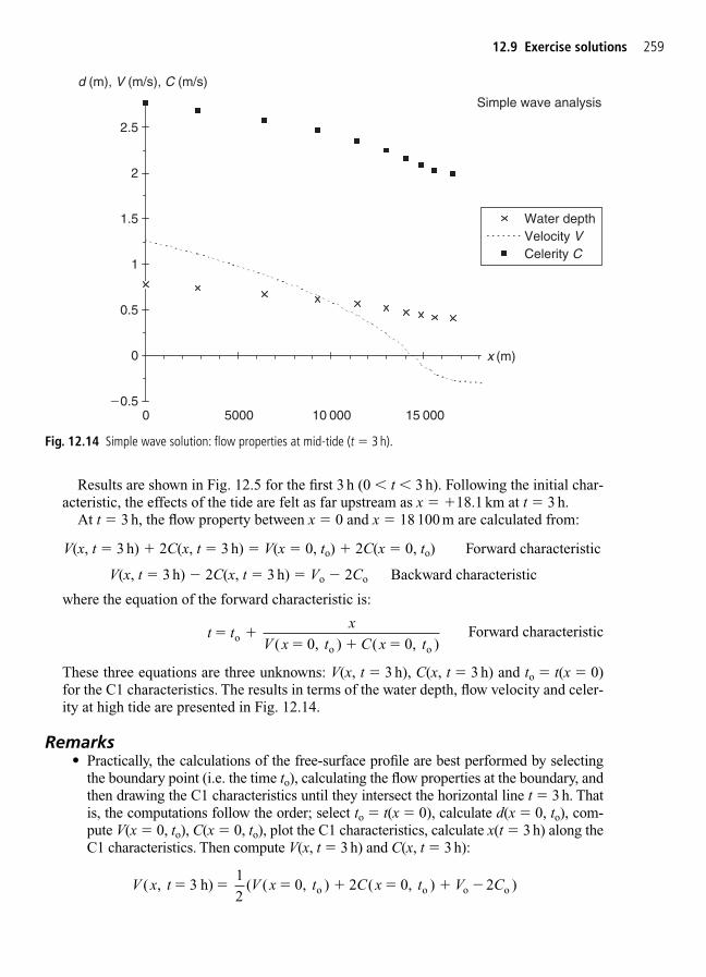
Results are shown in Fig. 12.5 for the first 3 h (0 � t � 3 h). Following the initial char-acteristic, the effects of the tide are felt as far upstream as x � 18.1 km at t � 3 h.

At t � 3 h, the flow property between x � 0 and x � 18 100 m are calculated from:

V(x, t � 3 h) 2C(x, t � 3 h) � V(x � 0, to) 2C(x � 0, to) Forward characteristic

V(x, t � 3 h) � 2C(x, t � 3 h) � Vo � 2Co Backward characteristic

where the equation of the forward characteristic is:

Forward characteristic

These three equations are three unknowns: V(x, t � 3 h), C(x, t � 3 h) and to � t(x � 0)for the C1 characteristics. The results in terms of the water depth, flow velocity and celer-ity at high tide are presented in Fig. 12.14.

Remarks• Practically, the calculations of the free-surface profile are best performed by selecting

the boundary point (i.e. the time to), calculating the flow properties at the boundary, andthen drawing the C1 characteristics until they intersect the horizontal line t � 3 h. Thatis, the computations follow the order; select to � t(x � 0), calculate d(x � 0, to), com-pute V(x � 0, to), C(x � 0, to), plot the C1 characteristics, calculate x(t � 3 h) along theC1 characteristics. Then compute V(x, t � 3 h) and C(x, t � 3 h):

V x t V x t C x t V C( , 3 h) 12

( ( 0, 2 ( 0, 2o o o o� � � � �) ) )

t tx

V x t C x t

( 0, ) ( 0, )oo o

� � �

12.9 Exercise solutions 259

�0.5

0

0.5

1

1.5

2

2.5

0 5000 10 000 15 000

Water depthVelocity VCelerity C

x (m)

Simple wave analysis

d (m), V (m/s), C (m/s)

Fig. 12.14 Simple wave solution: flow properties at mid-tide (t � 3 h).

Lastly the flow depth equals d � C2/g.• In Fig. 12.14, note that the velocity is positive (i.e. upriver flow) for x � 14.4 km at

t � 3 h.• Note that the C2 characteristics lines are not straight lines.• A relevant example is Henderson (1966, pp. 192–294).

9. The problem may be analysed as a simple wave. The initial flow conditions are: Vo � 0and Co � 3.7 m/s. Let select a coordinate system with x � 0 at the gate and x positive inthe upstream direction. In the (x, t) plane, the equation of the initial forward characteris-tics (issuing from x � 0 and t � 0) is given:

At t � 1 h, the extent of the influence of the gate operation is 13.3 km.10. The simple wave problem corresponds to a negative surge. In absence of further infor-

mation, the flume is assumed wide rectangular.Let select a coordinate system with x � 0 at the gate and x positive in the upstream

direction. The initial flow conditions are: V0 � � 0.9 and C0 � 4.0 m/s. In the (x, t) plane,the equation of the initial forward characteristics (issuing from x � 0 and t � 0) is given:

At t � 10 min, the maximum extent of the disturbance is x � 1870 m. That is, the zoneof quiet is defined as x � 1.87 km.

At the gate (x � 0), the boundary condition is: d(x � 0, to " 0) � 1.65 m, d(x � 0,to) � 1.65 � 8.33 �10�4to, for 0 � to � 960 s, and d(x � 0, to � 960 s) � 0.85 m. Thesecond flow property is calculated using the backward characteristics issuing from theinitial forward characteristics and intersecting the boundary at t � to:

V (x � 0, to) � Vo 2(C (x � 0, to) � Co) Backward characteristics

where C (x, to) � ��gd(x���0,�to�).At t � 10 min, the flow property between x � 0 and x � 1.87 km are calculated from:

V (x, t � 600) 2C (x, t � 600) � V (x � 0, to) 2C (x � 0, to)Forward characteristics

V (x, t � 600) � 2C (x, t � 600) � Vo � 2Co Backward characteristics

where the equation of the forward characteristics is:

Forward characteristics

These three equations are three unknowns: V (x, t � 600), C (x, t � 600) andto � t(x � 0) for the C1 characteristics. The results of the calculation at t � 12 min arepresented in Table 12.2 and Fig. 12.15.

t tx

V x t C x t

( 0, ( 0, oo o

� � �) )

dd

1

0.32 s/m

o o

tx V C

�

�

dd

1

0.27 s /m

o o

tx V C

�

�

C x t V x t C x t V C( , 3 h) 14

( ( 0, 2 ( 0, 2o o o o� � � � � ) ) )

260 Unsteady open channel flows: 2. Applications

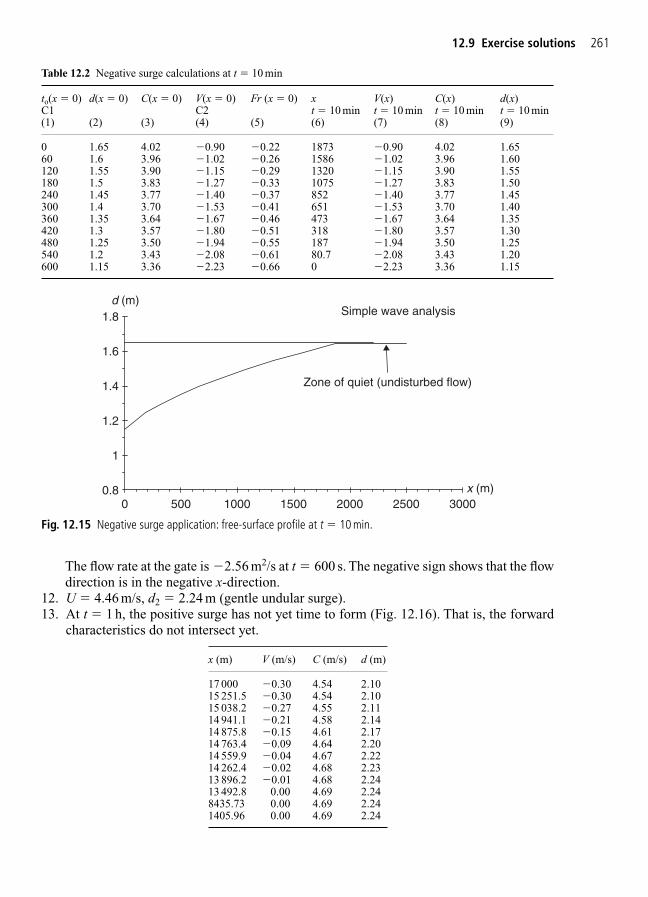
The flow rate at the gate is �2.56 m2/s at t � 600 s. The negative sign shows that the flowdirection is in the negative x-direction.

12. U � 4.46 m/s, d2 � 2.24 m (gentle undular surge).13. At t � 1 h, the positive surge has not yet time to form (Fig. 12.16). That is, the forward

characteristics do not intersect yet.

12.9 Exercise solutions 261

Table 12.2 Negative surge calculations at t � 10 min

to(x � 0) d(x � 0) C(x � 0) V(x � 0) Fr (x � 0) x V(x) C(x) d(x)C1 C2 t � 10 min t � 10 min t � 10 min t � 10 min(1) (2) (3) (4) (5) (6) (7) (8) (9)

0 1.65 4.02 �0.90 �0.22 1873 �0.90 4.02 1.6560 1.6 3.96 �1.02 �0.26 1586 �1.02 3.96 1.60120 1.55 3.90 �1.15 �0.29 1320 �1.15 3.90 1.55180 1.5 3.83 �1.27 �0.33 1075 �1.27 3.83 1.50240 1.45 3.77 �1.40 �0.37 852 �1.40 3.77 1.45300 1.4 3.70 �1.53 �0.41 651 �1.53 3.70 1.40360 1.35 3.64 �1.67 �0.46 473 �1.67 3.64 1.35420 1.3 3.57 �1.80 �0.51 318 �1.80 3.57 1.30480 1.25 3.50 �1.94 �0.55 187 �1.94 3.50 1.25540 1.2 3.43 �2.08 �0.61 80.7 �2.08 3.43 1.20600 1.15 3.36 �2.23 �0.66 0 �2.23 3.36 1.15

1

1.8

1.6

1.4

1.2

0.80 500 1000 1500 2000 2500 3000

x (m)

d (m)Simple wave analysis

Zone of quiet (undisturbed flow)

Fig. 12.15 Negative surge application: free-surface profile at t � 10 min.

x (m) V (m/s) C (m/s) d (m)

17 000 �0.30 4.54 2.1015 251.5 �0.30 4.54 2.1015 038.2 �0.27 4.55 2.1114 941.1 �0.21 4.58 2.1414 875.8 �0.15 4.61 2.1714 763.4 �0.09 4.64 2.2014 559.9 �0.04 4.67 2.2214 262.4 �0.02 4.68 2.2313 896.2 �0.01 4.68 2.2413 492.8 0.00 4.69 2.248435.73 0.00 4.69 2.241405.96 0.00 4.69 2.24

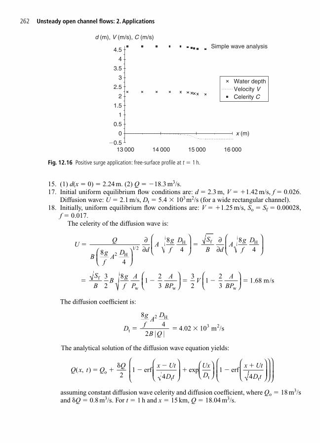
15. (1) d(x � 0) � 2.24 m. (2) Q � �18.3 m3/s.17. Initial uniform equilibrium flow conditions are: d � 2.3 m, V � 1.42 m/s, f � 0.026.

Diffusion wave: U � 2.1 m/s, Dt � 5.4 � 103m2/s (for a wide rectangular channel).18. Initially, uniform equilibrium flow conditions are: V � 1.25 m/s, So � Sf � 0.00028,

f � 0.017.The celerity of the diffusion wave is:

The diffusion coefficient is:

The analytical solution of the diffusion wave equation yields:

assuming constant diffusion wave celerity and diffusion coefficient, where Qo � 18 m3/sand �Q � 0.8 m3/s. For t � 1 h and x � 15 km, Q � 18.04 m3/s.

Q x t QQ x Ut

D t

UxD

x Ut

D t( , )

2 1 erf

4 exp 1 erf

4o

t t t

� �

��

�

D

gf

AD

B Qt

2 H

3 2

8

| | 4.02 10 m s� � �

42

/

UQ

Bgf

AD d

Agf

D S

B dA

gf

D

S

BB

gf

AP

ABP

VA

BP

8

8

8

32

81

23

32

1 23

1.68 m/s

2 H

H f H

f

w w w

� �

� � � � �

4

4 41 2

∂∂

∂∂

/

262 Unsteady open channel flows: 2. Applications

0

0.5

�0.5

1

1.5

2

2.5

3

3.5

4

4.5

13 000 14 000 15 000 16 000

Water depthVelocity VCelerity C

x (m)

Simple wave analysis

d (m), V (m/s), C (m/s)

Fig. 12.16 Positive surge application: free-surface profile at t � 1 h.

13

Unsteady open channel flows:3. Application to dam break wave

SummaryIn this chapter the Saint-Venant equations for unsteady open channel flows areapplied to the dam break wave problem. Basic applications include dam breakwave in horizontal and sloping channels, flash floods and tsunamis.

13.1 Introduction

During the 19th Century, major dam break catastrophes included the failures of the PuentesDam in 1802, Dale Dyke Dam in 1864, Habra Dam in 1881 and South Fork (Johnstown)Dam in 1889. In the 20th Century, three major accidents were the St Francis and Malpasset Damfailures in 1928 and 1959 respectively, and the overtopping of the Vajont Dam in 1963 (Fig. 13.1). Table 13.1 documents further accidents. These accidents yielded strong intereston dam break wave flows. A dam break is not only an engineering failure but, more import-antly, a human tragedy often with some political implications.

Completed in 1926, the St Francis Dam was a 62.5 m high curved concrete gravity damlocated about 72 km North of Los Angeles. The dam thickness was 4.9 m at the crest and53.4 m at the lowest base elevation. The dam was equipped with 11 spillway openings (2.8 m2

each) and five outlet pipes (diameter 0.7 m). The spillways discharged onto the downstreamstepped face of the dam (0.4 m step height). The reservoir began filling in 1926 and wasnearly full on the 5 March 1928. The volume of the reservoir was 46.9 Mm3 at that date.Although the dam site was investigated on the morning of the 12 March 1928 and nothingwas judged hazardous, the dam collapsed suddenly on the evening of the 12 March 1928between 11:57 and 11:58 p.m. The peak discharge just below the dam reached 14 200 m3/s.Four hundred and fifty people were killed by the flood wave. The dam failure was caused bya combination of a massive landslide on the left abutment and uplift pressure effects.Afterwards geological and geotechnical investigations revealed the very poor quality of the geological setting. During the collapse, a single erect monolith survived essentiallyunmoved from its original position (Fig. 13.1(a) and (b)). The remnant part was blasted on 23 May 1929.

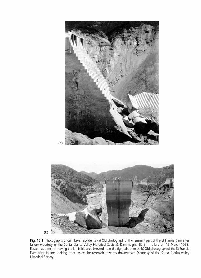
(a)

(b)

Fig. 13.1 Photographs of dam break accidents. (a) Old photograph of the remnant part of the St Francis Dam afterfailure (courtesy of the Santa Clarita Valley Historical Society). Dam height: 62.5 m, failure on 12 March 1928.Eastern abutment showing the landslide area (viewed from the right abutment). (b) Old photograph of the St FrancisDam after failure, looking from inside the reservoir towards downstream (courtesy of the Santa Clarita ValleyHistorical Society).

(c)

(d)

(e)

Fig. 13.1 (c) Remains of the Malpasset Dam in 1981. Dam height: 60 m, failure on 2 December 1959. View fromupstream looking downstream, with the right abutment on the top right of the photograph. (d) Left abutment of theMalpasset Dam in the late 1990s (courtesy of Didier Toulouze). (e) Möhne Dam shortly after the RAF raid on 16–17May 1943. Almost 1300 people died in the floods following the dam buster campaign, mostly inmates of a Prisonerof War (POW) camp just below the dam.

266 Unsteady open channel flows: 3. Application to dam break wave

Table 13.1 Examples of dam break failures and dam overtopping

Dam/reservoir Years of Date of Accident/failure Lives construction accident lost

(1) (2) (3) (4) (5)

Dam breakPuentes Dam, Spain 1785–1791 30 April Masonry dam break caused by a failure of 608

1802 wooden pile foundation.

Blackbrook Dam, UK 1795–1797 1799 Collapse caused by dam settlement and Nonespillway inadequacy.

South Fork (Johnstown) 1839 May 1889 Overtopping and break of earth dam caused Over Dam, USA by spillway inadequacy. 2000

Bilberry Dam, UK 1843 5 February Failure of earth dam caused by poor 811852 construction quality.

Dale Dyke Dam, UK 1863 11 March Earth embankment failure attributed to poor 1501864 construction work. Surge wave volume �0.9 Mm3.

Habra Dam, Algeria 1873 December Break of masonry gravity dam caused by 2091881 inadequate spillway capacity leading to

overturning. Note that the storm rainfall of 165 mm in one night lead to an estimated runoffof about three times the reservoir capacity.

Bouzey Dam, France 1878–1880 27 April Dam accident in 1884. Dam break in 1895. 851895

Austin Dam, USA 1892 7 April Dam break during overflow caused by –1900 foundation failure.

Minneapolis Mill Dam, 1893–1894 1899 Dam break during a small spill (caused by –USA cracks resulting from ice pressure on the dam).

Dolgarrog Dams, UK 1911/1910s 1925 Sequential failure of two earth dams following 25undermining of the upper structure.

Möhne Dam, Germany 1913 16–17 May RAF bombing of the dam to stop hydro-electricity 13001943 production.

Moyie River Dam, USA 1920s 1925 Failure of the left abutment and spillway (caused Noneby undermining) during large flood. Arch wall still standing.

Lake Lanier Dam, USA 1925 21 January Failure by undermining and overturning of the None1926 left abutment. Arch wall still standing.

St Francis Dam, USA 1926 1928 Dam break (caused by foundation failures). 450

Malpasset Dam, France 1957–1958 2 December Arch dam break caused by uplift pressures. Over 1959 300

Belci Dam, Romania 1958–1962 1991 Dam overtopping and breach (caused by a 97failure of gate mechanism).

Teton Dam, USA 1976 5 June 1976 Dam failure caused by cracks and piping in 11the embankment near completion.

Tous Dam, Spain 1977 1982 Dam break (following an overtopping; collapse Nonecaused by an electrical failure).

Cité de la Jonquière July 1996 Right abutment overtopping during floods of NoneDam, Canada the Rivière aux Sables, Saguenay region.

Lake Ha! Ha! Dam, – July 1996 Dam overtopping caused by extreme rainfalls NoneCanada (18–22 July) in the Saguenay region.

Zeyzoun (or Zayaoun) 1996 4 June 2002 Embankment dam cracks, releasing about 71 Mm3 22Dam, Syria of water. A 3.3 m high wall of water rushed through

the villages submerging over 80 km2. The final breach was 80 m wide.

(Contd)

The Malpasset Dam was a double-curvature arch dam located on the Reyran Riverupstream of Fréjus, southern France. The town of Fréjus is on the site of an ancient naval basefounded by Julius Caesar about BC 50, known originally as Forum Julii. Designed by AndréCoyne (1891–1960), the Malpasset Dam was 60 m high, the wall thickness was 6.0 and 1.5 mat base and at crest respectively, and the opening angle of the arch was 135°. The reservoirwas an irrigation water supply. Completed in 1954, the reservoir was not full until lateNovember 1959. On 2 December 1959 around 9:10 p.m., the dam wall collapsed completely.More than 300 people died in the catastrophe. Field observations showed that the surgingwaters formed a 40 m high wave at 340 m downstream of the dam site and the wave heightwas still about 7 m about 9 km downstream (Faure and Nahas 1965). The dam break wavetook about 19 min to cover the first 9 km downstream of the dam site. (Relatively accuratetime records were obtained from the destruction of a series of electrical stations located in thedownstream valley.) The dam collapse was caused by uplift pressures in faults of the gneissrock foundation which lead to the complete collapse of the left abutment (Fig. 13.1(d)).

Designed by Carlo Semenza (1893–1961), the Vajont Dam (Italy) is a double-curvaturearch structure, built between 1956 and 1960. The 262 m high reinforced-concrete dam cre-ated a 169 � 106m3 reservoir which was filled up by a major landslide on 9 October 1963.The reservoir waters overtopped the dam and the flood wave devastated the downstream val-ley. More than 2000 people died in the catastrophe. Little damage was done however to thedam itself which is still standing and used despite a drastically reduced storage capacity. At the dam toe, the overtopping nappe reached velocities in excess of 70 m/s before impact.Although the bed friction slowed down the resulting wave, the warning time was too short.

Discussion: man-made dam failuresDuring armed conflicts, man-made flooding of an army or a city was carried out by buildingan upstream dam and destroying it. Historical examples include the Assyrians (Babylon, Iraq BC 689), the Spartans (Mantinea, Greece BC 385–384), the Chinese (Huai River, AD 514–515), the Russian army (Dnieprostroy Dam, 1941) (Dressler 1952, Smith 1971,Schnitter 1994). It may be added the aborted attempt to blow up Ordunte Dam, during theSpanish civil war, by the troops of General Franco, and the anticipation of German Damdestruction at the German–Swiss border to stop the crossing of the Rhine River by the AlliedForces in 1945 (Ré 1946). A related case is the air raid on the Möhne Dam in the Ruhr Basinconducted by the British, in 1943, during the dam buster campaign (Fig. 13.1(e)). In 1961,

13.1 Introduction 267

Table 13.1 (Contd)

Dam/reservoir Years of Date of Accident/failure Lives construction accident lost

(1) (2) (3) (4) (5)

Glashütte Dam, Germany 1953 12 August Embankment dam overtopping during very large None2002 flood because of inadequate spillway capacity.

Dam overtoppingWarren Dam, Australia 1916 1917 Dam overtopped (no damage). None

Palagnedra Dam, 1952 1978 Dam overtopping (caused by a combination of 24Switzerland large flood and large volume of debris).

Vajont Dam, Italy 1956–1960 9 October Dam overtopping following a massive landslide Over 1963 into the 169 � 106m3 reservoir. 2000

References: Smith (1971), Schnitter (1994), Chanson et al. (2000).

the Swiss army blew up with explosives a concrete arch dam to document the flooding of thedownstream valley (Lauber 1997).

Dyke destruction and associated flooding played also a role in several wars. For example,the war between the cities of Lagash and Umma (Assyria) around BC 2500 was fought for thecontrol of irrigation systems and dykes; in 1938, the Chinese army destroyed dykes along the Huang Ho River (Yellow River) to slow down the Japanese army.

13.2 Dam break wave in a horizontal channel

13.2.1 Dam break in a dry channel

Considering an ideal dam break surging over a dry river bed, the method of characteristicsmay be applied to solve completely the wave profile as first proposed by Ritter in 1892 (e.g.Henderson 1966, Montes 1998). Interestingly, Ritter’s work was initiated by the South ForkDam’s (Johnstown) catastrophe (Table 13.1).

268 Unsteady open channel flows: 3. Application to dam break wave

do

x

y

Ideal dam break(downstream dry bed)

Idealfluid

Real fluid

Negative wave

do49 U

Removeddam wall

t

x

Initialbackward

characteristic

Backwardcharacteristic

Forwardcharacteristic

Trajectoryof dam break

front

Zone of quiet

1 1

Co 2Co

E1F1

G1

Fig. 13.2 Sketch of dam break wave in a dry horizontal channel.

The dam break may be idealized by a vertical wall that is suddenly removed (Fig. 13.2).After the removal of the wall, a negative wave propagates upstream and a dam break wavemoves downstream. Although there is considerable vertical acceleration during the initialinstants of fluid motion, such acceleration is not taken into account by the method of charac-teristics and the pressure distributions are assumed hydrostatic. For an ideal dam break overa dry horizontal channel, the basic equations are those of the simple wave (Chapter 12,Section 12.3.1):

Forward characteristics (13.1a)

Backward characteristics (13.1b)

along:

Forward characteristics C1 (13.2a)

Backward characteristics C2 (13.2b)

The instantaneous dam break creates a negative wave propagating upstream into a fluid atrest with known water depth do. In the (x, t) plane, the initial negative wave characteristic hasa slope dt/dx � �1/Co where Co � �gdo

—–assuming a rectangular channel (Fig. 13.2).

The forward characteristics can be drawn issuing from the initial backward characteristicfor t � 0 and intersecting the trajectory of the leading edge of the dam break wave front (Fig.13.2, trajectory E1–F1). The forward characteristic satisfies:

(13.3)

since V � Vo � 0 and C � Co � �gdo—–

at the point E1 (Fig. 13.2).At the leading edge of the dam break wave front, the water depth is zero, hence C � 0, and

the propagation speed of the dam break wave front equals:

Ideal dam break (13.4)

Considering any backward characteristics issuing from the dam break wave front (Fig.13.2, trajectory F1–G1), the C2 characteristics is a straight line because the initial backwardcharacteristics is a straight line (Chapter 12, Section 12.3.1). The inverse slope of the back-ward characteristics is a constant:

using equation (13.3). The integration of the inverse slope gives the water surface profile atthe intersection of the C2 characteristics with a horizontal line t � constant (Fig. 13.2, pointG1). That is, at a given time, the free-surface profile between the leading edge of the negativewave and the wave front is a parabola:

(13.5a)xt

gd gd gdxt

gd 3 for 2o o o� � � " "2

dd

2 3oxt

V C C C� � � �

U C gd 2 o o� � 2

V C V C C 2 2 o o o � � 2

dd

xt

V C� �

dd

xt

V C�

DD

) 0t

V C( � �2

DD

) 0t

V C( �2

13.2 Dam break wave in a horizontal channel 269

At the origin (x � 0), equation (13.5a) predicts a constant water depth:

(13.6)

Similarly the velocity at the origin is deduced from equation (13.3):

(13.7)

After dam break, the flow depth and velocity at the origin are both constants, and the waterdischarge at x � 0 equals:

(13.8)

where W is the channel width.

Q x d gd W( 0) 827

o o� �

V x gd( 0)23 o� �

d x d( 0) 49 o� �

270 Unsteady open channel flows: 3. Application to dam break wave

DiscussionImportant contributions to the dam break wave problem in a dry horizontal channelinclude Ritter (1892), Schoklitsch (1917), Ré (1946), Dressler (1952, 1954) andWhitham (1955). The above development is sometimes called Ritter’s theory.Calculations were performed assuming a smooth rectangular channel, an infinitely longreservoir and for a quasi-horizontal free surface. That is, bottom friction is zero and thepressure distribution is hydrostatic. Experimental results (e.g. Schoklitsch 1917, Faureand Nahas 1961, Lauber 1997) showed that the assumptions of hydrostatic pressure dis-tributions and zero friction are reasonable, but for the initial instants and at the leadingtip of the dam break wave.

Bottom friction affects significantly the propagation of the leading tip. Escande et al.(1961) investigated specifically the effects of bottom roughness on dam break wave in anatural valley. They showed that, with a very rough bottom, the wave celerity could beabout 20–30% lower than for a smooth bed. The shape of a real fluid dam break wavefront is sketched in Fig. 13.2 and experimental results are presented in Fig. 13.6 (seeSection 13.3.1).

Notes1. The above development, called Ritter’s theory, was developed for a frictionless hori-

zontal rectangular channel initially dry and an infinitely long reservoir. The free sur-face is also assumed to be quasi-horizontal.

2. The assumption of hydrostatic pressure distributions has been found to be reason-able, but for the initial instants: i.e. t � 3�do/g

—––(Lauber 1997).

3. Ritter’s theory implies that the celerity of the initial negative wave is U � ��gdo—–

Experimental observations suggested however that the real celerity is aboutU � ��2

—�gdo—–

(Lauber 1997, Leal et al. 2001). It was suggested that the differencewas caused by streamline curvature effects at the leading edge.

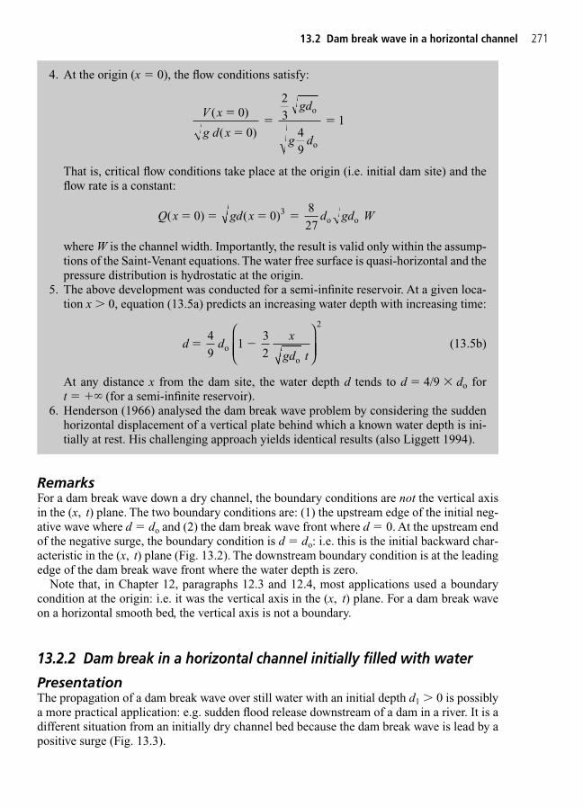
RemarksFor a dam break wave down a dry channel, the boundary conditions are not the vertical axisin the (x, t) plane. The two boundary conditions are: (1) the upstream edge of the initial neg-ative wave where d � do and (2) the dam break wave front where d � 0. At the upstream endof the negative surge, the boundary condition is d � do: i.e. this is the initial backward char-acteristic in the (x, t) plane (Fig. 13.2). The downstream boundary condition is at the leadingedge of the dam break wave front where the water depth is zero.

Note that, in Chapter 12, paragraphs 12.3 and 12.4, most applications used a boundarycondition at the origin: i.e. it was the vertical axis in the (x, t) plane. For a dam break waveon a horizontal smooth bed, the vertical axis is not a boundary.

13.2.2 Dam break in a horizontal channel initially filled with water

PresentationThe propagation of a dam break wave over still water with an initial depth d1 � 0 is possiblya more practical application: e.g. sudden flood release downstream of a dam in a river. It is adifferent situation from an initially dry channel bed because the dam break wave is lead by apositive surge (Fig. 13.3).

13.2 Dam break wave in a horizontal channel 271

4. At the origin (x � 0), the flow conditions satisfy:

That is, critical flow conditions take place at the origin (i.e. initial dam site) and theflow rate is a constant:

where W is the channel width. Importantly, the result is valid only within the assump-tions of the Saint-Venant equations. The water free surface is quasi-horizontal and thepressure distribution is hydrostatic at the origin.

5. The above development was conducted for a semi-infinite reservoir. At a given loca-tion x � 0, equation (13.5a) predicts an increasing water depth with increasing time:

(13.5b)

At any distance x from the dam site, the water depth d tends to d � 4/9 � do fort � � (for a semi-infinite reservoir).

6. Henderson (1966) analysed the dam break wave problem by considering the suddenhorizontal displacement of a vertical plate behind which a known water depth is ini-tially at rest. His challenging approach yields identical results (also Liggett 1994).

d dx

gd t

49

1 32o

o

� �

2

Q x gd x d gd W( 0) ( 0) 827

3o o� � � �

V x

g d x

gd

g d

( 0)

( 0)

49

1o

o

�

�� �

23

272 Unsteady open channel flows: 3. Application to dam break wave

Quasi-steady flow analogy at the surge front(as seen by an observer travelling at the surge velocity)

Ud1

d2U � V2

t

x

Initialbackward

characteristic

Forwardcharacteristic

Trajectoryof positive surge

Zone of quiet

1

1

Co

Co

Removeddamwall

do

d2 d1 x

yIdeal dam break

(initial downstream water level)

Advancing positive surge

Negative wave

Still water

V2

V2 � C2

U

UE1 E2 E3

1

Fig. 13.3 Sketch of dam break wave in a horizontal channel initially filled with water for d1 � 0.1383 � do.

The basic flow equations are the characteristic system of equations (paragraph 13.2.1), andthe continuity and momentum equations across the positive surge front. That is:

Forward characteristics (13.1a)

Backward characteristics (13.1b)DD

) 0 along dd

t

V Cxt

V C( � � � �2

DD

) 0 along dd

t

V Cxt

V C( � � 2

Continuity equation (13.9a)

Momentum equation (13.10a)

where U is the positive surge celerity for an observer fixed on the channel bank, and the sub-scripts 1 and 2 refer respectively to the flow conditions upstream and downstream of the posi-tive surge front: i.e. initial flow conditions and new flow conditions behind the surge front(Fig. 13.3).

Immediately after the dam break, a negative surge propagates upstream into a fluid at restwith known water depth do. In the (x, t) plane, the initial negative wave characteristics has aslope dt/dx � �1/Co where Co � �gdo

—–assuming a rectangular channel (Fig. 13.3). The ini-

tial backward characteristics is a straight line, hence all the C2 characteristics are straightlines (Chapter 12, Section 3.3.1).

For t � 0, the forward characteristics issuing from the initial backward characteristics cannotintersect the downstream water level (d � d1) because it would involve a discontinuity in veloc-ity. The velocity is zero in still water (V1 � 0) but, on the forward characteristics, it satisfies:

(13.3)

Such a discontinuity can only take place as a positive surge which is sketched in Fig. 13.3.

Detailed solutionConsidering a horizontal, rectangular channel, the water surface is horizontal upstream of theleading edge of the negative wave (Fig. 13.3, point E1). Between the leading edge of the neg-ative wave (point E1) and the point E2, the free-surface profile is a parabola:

(13.5a)

Between the point E2 and the leading edge of the positive surge (point E3), the free-surfaceprofile is horizontal. The flow depth d2 and velocity V2 satisfy equations (13.9a) and (13.10a),as well as the condition along the C1 forward characteristics issuing from the initial negativecharacteristics and reaching point E2:

Forward characteristics (13.3)

Equations (13.3), (13.9a) and (13.10a) form a system of three equations with threeunknowns V2, d2 and U. The system of equations may be solved graphically (Fig. 13.4).Figure 13.4 shows U/�gd

—1, d2/d1 and V2/�gd

—2, (right axis), and (V2 � C2)/�gd

—1 (left axis) as

functions of the ratio do/d1.Once the positive surge forms (Fig. 13.3), the locations of the points E2 and E3 satisfy

respectively:

xE2 � (V2 � C2)t

xE3 � U t

where C2 � �gd—

1 for a rectangular channel. Figure 13.4 shows that U � (V2 � C2) for t � 0and 0 � (d1/do) � 1. That is, the surge front (point E3) advances faster than the point E2.

V gd gd2 2 o 2 2 �

xt

gd gd x x x 2 3o E E2� � " "1

V C V C C 2 2 o o o � � 2

d U V d gd gd2 22

12( U

12

12

� � � �) 12

22

d U d U V1 2 2 ( � � )

13.2 Dam break wave in a horizontal channel 273

Montes (1998) showed that the surge celerity satisfies:

(13.11)

where

The flow conditions behind the surge front are then deduced from the quasi-steady flowanalogy (Chapter 12, Section 12.4.2).

XUgd

12

1 8 12

1

� �

dd

U

gd XXo

1 1

12

1 1

� �

274 Unsteady open channel flows: 3. Application to dam break wave

�4.00

�2.00

0.00

2.00

4.00

6.00

8.00

1 21 41 61 810

2

4

6

8

10

12

14

16

18

U/ (gd1), d2/d1, V2/ (gd2)

U/ (gd1)

(V2 – C2)/ (gd1)

(V2 � C2)/ (gd1)

V2/ (gd2)

U/ (gd1)

do/d1

d2/d1

d2/d1

V2/ (gd2)

Fig. 13.4 Graphical solution of the flow conditions for a dam break wave in a horizontal channel initially filled with water.

Notes1. The above equations were developed for initially still water (V1 � 0). Experimental

observations compared well with the above development and they showed that bot-tom friction is negligible.

2. Figure 13.4 is valid for 0 � (d1/do) � 1.3. The flow depth downstream of (behind) the positive surge is deduced from the continu-

ity and momentum equations. d2 is independent of the time t and distance x. Practically,the flow depth d2 is a function of the depths d1 and do. It may be correlated by:

dd

dd

2

o

1

o

0.9319671�

0 371396.

13.2 Dam break wave in a horizontal channel 275

Good agreement was observed between large-size experimental data and the abovecorrelation (e.g. Chanson et al. 2000).

4. Equation (13.11) may be empirically correlated by:

5. Figure 13.3 illustrates the solution of the Saint-Venant equations. It shows some dis-continuities in terms of free-surface slope and curvatures at the points E1 and E2.Such discontinuities are not observed experimentally and this highlights some limi-tation of the Saint-Venant equations.

ApplicationA 35 m high dam fails suddenly. The initial reservoir height was 31 m above the downstream channel invert and the downstream channel was filled with 1.8 m of waterinitially at rest. (1) Calculate the wave front celerity, and the surge front height. (2) Calculate the wave front location and free-surface profile 2 min after failure. (3) Predictthe water depth 10 min after gate opening at two locations: x � 2 km and x � 4 km.Assume an infinitely long reservoir and a horizontal, smooth channel.

SolutionThe downstream channel was initially filled with water at rest. The flow situation issketched in Fig. 13.3. The x coordinate is zero (x � 0) at the dam site and positive in thedirection of the downstream channel. The time origin is taken at the dam collapse.

First the characteristic system of equation, and the continuity and momentum prin-ciples at the wave front must be solved graphically using Fig. 13.4 or theoretically.

Using Fig. 13.4, the surge front celerity is: U/�gd1—–

� 4.3 and U � 18.1 m/s.At the wave front, the continuity and momentum equations yield:

Hence d2 � 10.14 m

Equation (12.33) may be rewritten:

Hence V2 � 14.9 m/s

Note that these results are independent of time.At t � 2 min, the location of the points E1, E2 and E3 sketched in Fig. 13.3 is:

x U tE 2.2 km3 � �

x V gd tE2 2 2 0.59 km � � � ( )x gd tE1 o 2.1 km � � � �

V

gd

dd

2

2

o

2

2 1 1.5� � �

dd

Ugd

2

1

2

1

12

1 8 1 5.63� � �

U

gd

dd

dd

1

1

o

1

o

0.635 45 0.328 6

0.002 51

�

0 65167

0 65167

.

.

Extension to non-zero initial flow velocityThis development may be easily extended for initial flow conditions with a non-zero, con-stant initial velocity V1. Equations (13.3), (13.9a) and (13.10a) become:

Forward characteristics (13.3)

Continuity equation (13.9b)

Momentum equation (13.10b)

DiscussionFigure 13.3 sketches a situation where the point E2 is located downstream of the initial damwall. At the origin, the water depth and velocity are respectively (paragraph 13.2.1):

(13.6)

(13.7)V x gd( 0) 23 o� �

d x d( 0) 49 o� �

d U V d U V gd gd2 2 1 1( ( 12

12

� � � � �) )2 212

22

d U V d U V1 1 2 2( ( � � �) )

V gd gd2 2 o 2 2 �

276 Unsteady open channel flows: 3. Application to dam break wave

Between the points E1 and E2, the free-surface profile is a parabola:

(13.5)

The free-surface profile at t � 2 min is:

x (m) �5000 �2100 �1000 0 595 2178 2178 5000d (m) 31 31 21.1 13.7 10.14 10.14 1.8 1.8Remark Point E1 Point E2 Point E3

Lastly d(x � 2 km, t � 10 min) � 11.3 m and d(x � 4 km, t � 10 min) � 10.1 m.

Remarks1. As d1/do � 0.138, the water depth and flow rate at the dam site equal:

2. For a sudden dam break wave over an initially dry channel, the wave front celerity wouldbe 35 m/s (equation (13.4), for an ideal dam break on a smooth frictionless channel).

q x gd( 0) 827

160m /so3 2� � �

d x d( 0) 49

13.7 mo� � �

xt

gd gd x x x 2 3 o E E� � " "1 2

Another situation is sketched in Fig. 13.5 where the point E2 is located upstream of thedam wall. Between these two situations, the limiting case is a fixed point E2 at the origin.This occurs for

For d1/do � 0.1383, the flow situation is sketched in Fig. 13.3. For d1/do � 0.1383, the pointE2 is always located upstream of the origin and the flow pattern is illustrated in Fig. 13.5.

dd

1

o

0.1383�

13.2 Dam break wave in a horizontal channel 277

C2 – V2

t

x

Initialbackward characteristic

Trajectoryof positive surge

Zone of quiet

1

1

Co

dod2 d1

x

y Advancing positive surge

Still water

V2

U

U1

E1

E2

E3

Fig. 13.5 Sketch of a dam break wave in horizontal channel initially filled with water for 0.1383 � d1/do � 1.

ApplicationDemonstrates that the intersection of the forward characteristics issuing from the initialcharacteristics with the horizontal free-surface behind the positive surge (i.e. point E2,Fig. 13.3) is at the origin (x � 0) if and only if:

SolutionIn the limiting case for which the point E2 is at the origin, the water depth and velocityat the origin are respectively:

d x d d d( 0) 49

o E2 2� � � �

dd

1

o

0.1383�

13.3 Effects of flow resistance

13.3.1 Flow resistance effect on dam break wave on horizontal channel

For a dam break wave in a dry horizontal channel, observations showed that Ritter’s theory(paragraph 13.2.1) is valid but for the leading tip of the wave front. Experimental data indi-cated that the wave front has a rounded shape and its celerity U is less than 2Co (e.g.Schoklitsch 1917, Dressler 1954, Faure and Nahas 1961). Escande et al. (1961) investigatedspecifically the effects of bottom roughness on dam break wave in a natural valley. They

278 Unsteady open channel flows: 3. Application to dam break wave

where d2 and the V2 are the flow velocity behind (downstream of) the positive surge.First the flow conditions at the origin satisfies V2/�gd2

—–� 1

Second the continuity and momentum equations across the positive surge give:

where U is the celerity of the positive surge (Chapter 12). One of the equations may besimplified into:

This system of non-linear equations may be solved by a graphical method and by test-and-trial. The point E2 is at the origin for:

Notes1. For d1/do � 0.1383, the discharge at the origin is a constant independent of time:

(13.8)

2. For d1/do � 0.1383, the discharge at the origin is also a constant independent of thetime. But the flow rate at x � 0 becomes a function of the flow depth d2 and it is lessthan 8/27�g

—Wdo

3/2. At the limit Q(x � 0) � 0 for d1 � do.

Q x d gd W( 0) 827

o o� �

dd

1

o

0.1382701411�

U

gd dd

dd

1 1

o

1

o

1

278

�

�32

1 2 3 2

/ /

U V

gd

U

gd

Ugd

dd

U

gd

dd

2

1 8 1

278

12

2

3/2

1

2

1

1

o 1

1

2

��

�

� � �

3 2

3 2

/

/

dd

Ugd

dd

2

1

2

1

o

1

12

1 8 1 � � �

49

V x gd V V( 0) 23

o E2 2� � � �

showed that, with a very rough bottom, the wave celerity could be about 20–30% lower than fora smooth bed. Faure and Nahas (1965) conducted both physical and numerical modelling of thecatastrophe of the Malpasset Dam (Fig. 13.1(c) and (d)). In their study, field observations werebest reproduced with a Gauckler–Manning coefficient nManning � 0.025–0.033 s/m1/3.

Figure 13.6 compares the simple-wave theory (zero friction) with measured dam breakwave profiles, and it illustrates the round shape of the leading edge. Dressler (1952) andWhitham (1955) proposed analytical solutions of the dam break wave that include the effectsof bottom friction, assuming constant friction coefficient. Some results are summarized inTable 13.2 while their respective theories are discussed below.

13.3 Effects of flow resistance 279

0

0.2

0.4

0.6

0.8

1

�1 �0.5 0 0.5 1 1.5 2x/t (gdo)

d/do Dam break wave profile

Simple wave theory

Dressler/Whitham

SchoklitschFaure and Nahas

Fig. 13.6 Comparison of the dam break wave profile in an initially dry horizontal channel with and without bottomfriction.

Table 13.2 Analytical solutions of dam break wave with and without bottom friction

Parameter Simple wave Dressler (1952) Whitham (1955) RemarksRitter’s solution

(1) (2) (3) (4) (5)

Wave front – For t � ts smallcelerity U

–

Note: Theoretical results obtained for an initially dry horizontal channel.

U gd 2 o�U

gd

ft

g

d

o

so

2

3.4528

� �

Q x

W

( 0��

) 827

gdo3 8

27

1 0.2398

o3

o

gd

f g

dt

�

�

Location of critical flow conditions

x � 0 x

d

f g

dt

o o

8 � 0 395.

–

Dam break wave calculations with flow resistanceThe theoretical solutions of Dressler and Whitham give very close results and they are in rea-sonable agreement with experimental data (Fig. 13.6). Both methods yield results close to thesimple-wave solution but next to the leading tip.

Dressler (1952) used a perturbation method. His first order correction for the flow resist-ance gives the velocity and celerity at any position:

where f is the Darcy friction factor. The functions F1 and F2 are respectively:

Dressler compared successfully his results with the data of Schoklitch (1917) and his owndata (Dressler 1954).

At t � ts, the location xs of the dam break wave front satisfies:

Further results are summarized in Table 13.2.

f gd

t

x

t gd

x

t gd

x

t gd

8

2

3

2

3

63 2

os

s

s o

s

s o

s

s o

�

�

�

�

�

1 6

54

7

3 2

1 2

/

Fx

t gd

x

t gd2

o

o

6

5 2

23

4 3135

2 �

�

� �

3 2/

F

x

t gd

x

t gd

x

t gd1

oo

o

108

7 2

12

2

83

8 3189

2 ��

�

�

� �

2

3 2/

C

gd

x

t gdF

f gd

to o

2o

13

2

8

� �

V

gd

x

t gdF

f gd

to o

1o

23

1

8

�

280 Unsteady open channel flows: 3. Application to dam break wave

NoteFaure and Nahas (1965) conducted detailed physical modelling of the Malpasset Dam fail-ure using a Froude similitude. They used both undistorted and distorted scale models, aswell as a numerical model. For the distorted model, the geometric scaling ratios were:Xr � 1/1600 and Zr � 1/400. Field data were best reproduced in the undistorted physicalmodel (Lr � 1/400). Both numerical results and distorted model data were less accurate.

Whitham (1955) analysed the wave front as a form of boundary layer using an adaptationof the Pohlhausen method. For a horizontal dry channel, his estimate of the wave front celerity is best correlated by:

where f is the Darcy friction factor. Whitham commented that his work was applicable onlyfor U/�gdo

—–� 2/3. He further showed that the wave front shape would follow:

Wave front shape (x � xs)

for small.

13.3.2 Dam break wave down a sloping channel

Basic theoryConsidering the dam break wave down a sloping channel, the kinematic wave equation1 maybe solved analytically (Hunt 1982). Hunt’s analysis gives:

(13.12)

(13.13a)

(13.14)UV

V tL

x LL

V tLH

H s H 34

34

� �

2

xL d

H

dH

s 12

1s

dam

s

dam

� � �

32

V tL

dH

dH

H

s

dam

s

dam

1

�

�

2

3 2/

g d t f/ o /8

dd

f x xd

ft

gdo

s

o o

1/ 3

4

2 3.452 8

��

�

U

gdf gt

d

o 2

o

2

1 2.90724

�

8

0 4255

.

13.3 Effects of flow resistance 281

Notes1. For f � 0, Dressler’s solution is Ritter’s solution of the Saint-Venant equations.2. In an earlier development, Whitham (1955) assumed the shape of the wave front to follow:

where xs is the dam break wave front location, but he discarded the result as inaccurate (?).

dfg

U x x 4

s� �

1That is, the kinematic wave approximation of the Saint-Venant equations (Chapter 12, paragraph 12.5).

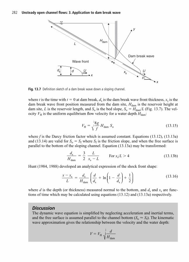
where t is the time with t � 0 at dam break, ds is the dam break wave front thickness, xs is thedam break wave front position measured from the dam site, Hdam is the reservoir height atdam site, L is the reservoir length, and So is the bed slope, So � Hdam/L (Fig. 13.7). The vel-ocity VH is the uniform equilibrium flow velocity for a water depth Hdam:

(13.15)

where f is the Darcy friction factor which is assumed constant. Equations (13.12), (13.13a)and (13.14) are valid for So � Sf where Sf is the friction slope, and when the free surface isparallel to the bottom of the sloping channel. Equation (13.13a) may be transformed:

For xs/L � 4 (13.13b)

Hunt (1984, 1988) developed an analytical expression of the shock front shape:

(13.16)

where d is the depth (or thickness) measured normal to the bottom, and ds and xs are func-tions of time which may be calculated using equations (13.12) and (13.13a) respectively.

x xL

dH

dd

dd

1

12

s s

dam s s

�� � ln

dH

Lx L

s

dam s

32

��

Vgf

H SH dam o 8

�

282 Unsteady open channel flows: 3. Application to dam break wave

DiscussionThe dynamic wave equation is simplified by neglecting acceleration and inertial terms,and the free surface is assumed parallel to the channel bottom (So � Sf). The kinematicwave approximation gives the relationship between the velocity and the water depth:

V Vd

H H

dam

�

x

y

xs

Dam break wave

LHdam

U

ux

d

Wave front

ds U

Fig. 13.7 Definition sketch of a dam break wave down a sloping channel.

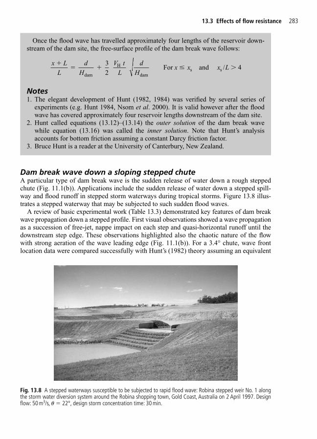
Dam break wave down a sloping stepped chuteA particular type of dam break wave is the sudden release of water down a rough steppedchute (Fig. 11.1(b)). Applications include the sudden release of water down a stepped spill-way and flood runoff in stepped storm waterways during tropical storms. Figure 13.8 illus-trates a stepped waterway that may be subjected to such sudden flood waves.

A review of basic experimental work (Table 13.3) demonstrated key features of dam breakwave propagation down a stepped profile. First visual observations showed a wave propagationas a succession of free-jet, nappe impact on each step and quasi-horizontal runoff until thedownstream step edge. These observations highlighted also the chaotic nature of the flowwith strong aeration of the wave leading edge (Fig. 11.1(b)). For a 3.4° chute, wave frontlocation data were compared successfully with Hunt’s (1982) theory assuming an equivalent

13.3 Effects of flow resistance 283

Once the flood wave has travelled approximately four lengths of the reservoir down-stream of the dam site, the free-surface profile of the dam break wave follows:

Notes1. The elegant development of Hunt (1982, 1984) was verified by several series of

experiments (e.g. Hunt 1984, Nsom et al. 2000). It is valid however after the floodwave has covered approximately four reservoir lengths downstream of the dam site.

2. Hunt called equations (13.12)–(13.14) the outer solution of the dam break wavewhile equation (13.16) was called the inner solution. Note that Hunt’s analysisaccounts for bottom friction assuming a constant Darcy friction factor.

3. Bruce Hunt is a reader at the University of Canterbury, New Zealand.

x LL

dH

V tL

dH

x x x L

32

For and / 4 dam

H

dams s

� � �

Fig. 13.8 A stepped waterways susceptible to be subjected to rapid flood wave: Robina stepped weir No. 1 alongthe storm water diversion system around the Robina shopping town, Gold Coast, Australia on 2 April 1997. Designflow: 50 m3/s, � � 22°, design storm concentration time: 30 min.

Darcy–Weisbach friction factor f � 0.05, irrespective of flow rate and chute configuration(Chanson 2003c, 2004d).

Second air–water flow measurements demonstrated quantitatively very strong flow aer-ation at the wave leading edge (see Discussion). The shape of the leading edge followedclosely Hunt’s (1984) inner solution. Unsteady air–water velocity profiles showed further thepresence of an unsteady turbulent boundary layer next to the invert.

284 Unsteady open channel flows: 3. Application to dam break wave

Notes1. In steady stepped chute flows, three flow regimes may be observed depending upon

the flow rate and step geometry: i.e. nappe flow, transition flow and skimming flow(e.g. Chanson 2001a). In a dam break wave flow down a stepped cascade, only oneflow regime was observed: i.e. a nappe flow consisting of a succession of free-fallingnappe, nappe impact and horizontal runoff (Fig. 11.1(c)).

2. Chanson (2001a, pp. 293–299) discussed other unsteady flow situations down steppedchutes, including roll wave phenomena and shock waves.

DiscussionDetailed unsteady air–water flow measurements were conducted in wave front leadingedge (Chanson 2003, 2004d). At the front of the wave, the instantaneous vertical distri-butions of void fraction in the horizontal runoff had a roughly linear shape:

where Y90 is the height where C � 0.90 and t is the time measured from the first waterdetection by a reference probe. For larger times t, the distributions of air concentrationwere best described by the diffusion model:

where K� and Do are functions of the mean air content only (Chapter 17). The data highlighted a major change in void fraction distribution shape for t �g/do

—–� 1.3

C K

yYD

yY

Dt

gd

1 tanh 2

13

1.3 2

o o o

� � � �

�

�90 90

3

3

Cy

Yt

gd

0.9 1.390 o

� � �0 1.

Table 13.3 Experimental conditions of dam break wave flow down a stepped chute

Experiment � (degree) h (m) Q(t � 0) (m3/s) do (m) Remarks(1) (2) (3) (4) (5) (6)

Chanson 3.4 0.143 0.019–0.075 0.12–0.30 10 horizontal steps (l � 2.4 m). (2003, 2004d) W � 0.5 m.

3.4 0.0715 0.03–0.075 0.16–0.30 18 horizontal steps (l � 1.2 m). W � 0.5 m. Detailed air–water flow measurements.

Brushes Clough 18.4 0.19 0.5 0.42 Inclined downward steps, Dam (Baker 1994) trapezoidal channel (2 m bottom

width).

Notes: h: step height; Q(t � 0): initial flow rate.

13.3 Effects of flow resistance 285

(Fig. 13.9). Possible explanations might include (a) a non-hydrostatic pressure field inthe leading front of the wave, (b) some change in air–water flow structure between theleading edge and the main flow associated with a change in rheological fluid properties,(c) a gas–liquid flow regime change with some plug/slug flow at the leading edge and ahomogenous bubbly flow region behind and (d) a change in boundary friction betweenthe leading edge and the main flow behind. All these mechanisms would be consistentwith high-shutter speed movies of leading edge highlighting very dynamic spray andsplashing processes.

x

Water droplets

Advancingwave front

Probe

Referenceprobe

y

y

C

y

C, VV

CUh

(a)

0

0.05

0.1

0.15

0.2

0.25

0 0.2 0.4 0.6 0.8 1

0–210 mm0–385 mm350–735 mm700–1085 mm

Steady flow

C

y /do Q(t � 0) � 55 L/s, Step 16, x� � 1.0 m, U � 2.14 m/s

�

2100–2485 mm

�� �

��

�

4200–4585 mm�

(b)

Fig. 13.9 Void fraction distributions behind the leading edge of surge front. (a) Definition sketch.(b) Experimental data: � � 3.4°, h � 0.07 m, U � 2.14 m/s, Step 16, x� � 1 m (horizontal runoff).

(mm) 0–210 0–385 350–735 700–1085 2100–2485 4200–4585

�X (m) � 0.210 0.385 0.385 0.385 0.385 0.385t�g/do

—–� 0.313 0.573 1.615 2.657 6.826 13.08

13.3.3 Further dam break wave conditions

Additional dam break wave conditions were experimentally studied. Chanson et al. (2000)investigated the propagation of a dam break wave downstream of a free-falling nappe impact.They observed strong splashing and mixing at the nappe impact, and their data showed consistently a greater wave front celerity than for the classical dam break analysis forx/do�30, where do is a function of the initial discharge. Khan et al. (2000) studied the effectsof floating debris. The results showed an accumulation of debris near the wave front and areduction of the front celerity both with and without initial water levels. Nsom et al. (2000)investigated dam break waves downstream of a finite reservoir in horizontal and slopingchannels with very viscous fluids. The dam break wave propagation was first dominated byinertial forces and then by viscous processes. In the viscous regime, the wave front locationfollowed:

where � is the bed slope and � is the fluid viscosity.

13.4 Embankment dam failures

13.4.1 Introduction

During the 19th Century, numerous embankment dams failed in Europe and North America.The two most common causes of failures were dam overtopping and cracking in the earthfill.The former was often caused by inadequate spillway facility. The latter resulted from a com-bination of bad understanding of basic soil mechanics, poor construction standards and pipingat the connection between bottom outlet and earth material. Figure 13.10(a) presents the rup-tured Dale Dyke Embankment Dam. The dam failure occurred rapidly as a result of piping inthe embankment. Figure 13.10(b) shows a failed tailings dam. The failure was caused byovertopping of runoff waters. At the nearby township of Merriespruit, 17 people were killedwhen another tailings dam failed on the night of 22 February 1994. At Merriespruit, water

xt

scos

��

�

286 Unsteady open channel flows: 3. Application to dam break wave

DISCUSSIONAnother related debris flow is the rockslide. Famous examples include the disastrousVajont slide on 9 October 1963 (paragraph 13.1). Another major rockslide was the MontGranier Cliff rockslide near Chambéry (France) in AD 1248. For both rockslides, it wasproposed that mechanical energy dissipated in heat inside the slip zone led to vaporizationof pore pressure, thus creating a cushion of zero or negligible friction (e.g. Vardoulakis2000).

In debris flow surges, large debris and big rocks are often observed ‘rolling’ and ‘float-ing’ at the wave front (e.g. Ancey 2000).

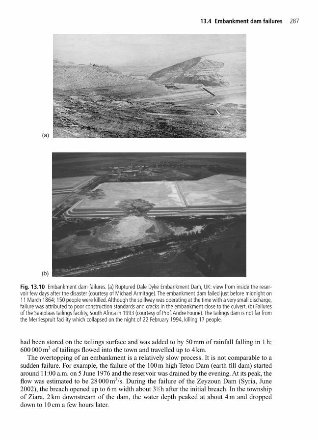
had been stored on the tailings surface and was added to by 50 mm of rainfall falling in 1 h;600 000 m3 of tailings flowed into the town and travelled up to 4 km.

The overtopping of an embankment is a relatively slow process. It is not comparable to asudden failure. For example, the failure of the 100 m high Teton Dam (earth fill dam) startedaround 11:00 a.m. on 5 June 1976 and the reservoir was drained by the evening. At its peak, theflow was estimated to be 28 000 m3/s. During the failure of the Zeyzoun Dam (Syria, June2002), the breach opened up to 6 m width about 31⁄2h after the initial breach. In the townshipof Ziara, 2 km downstream of the dam, the water depth peaked at about 4 m and droppeddown to 10 cm a few hours later.

13.4 Embankment dam failures 287

(a)

(b)

Fig. 13.10 Embankment dam failures. (a) Ruptured Dale Dyke Embankment Dam, UK: view from inside the reser-voir few days after the disaster (courtesy of Michael Armitage). The embankment dam failed just before midnight on11 March 1864; 150 people were killed.Although the spillway was operating at the time with a very small discharge,failure was attributed to poor construction standards and cracks in the embankment close to the culvert. (b) Failuresof the Saaiplaas tailings facility, South Africa in 1993 (courtesy of Prof. Andre Fourie). The tailings dam is not far fromthe Merriespruit facility which collapsed on the night of 22 February 1994, killing 17 people.

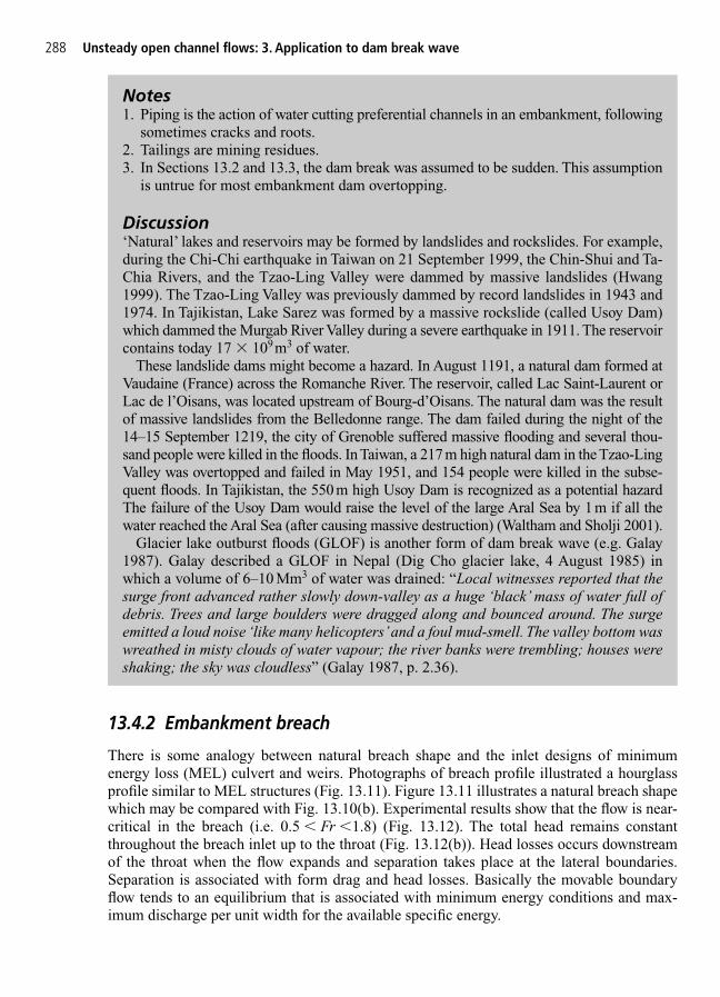
13.4.2 Embankment breach

There is some analogy between natural breach shape and the inlet designs of minimumenergy loss (MEL) culvert and weirs. Photographs of breach profile illustrated a hourglassprofile similar to MEL structures (Fig. 13.11). Figure 13.11 illustrates a natural breach shapewhich may be compared with Fig. 13.10(b). Experimental results show that the flow is near-critical in the breach (i.e. 0.5 � Fr �1.8) (Fig. 13.12). The total head remains constantthroughout the breach inlet up to the throat (Fig. 13.12(b)). Head losses occurs downstreamof the throat when the flow expands and separation takes place at the lateral boundaries.Separation is associated with form drag and head losses. Basically the movable boundaryflow tends to an equilibrium that is associated with minimum energy conditions and max-imum discharge per unit width for the available specific energy.

288 Unsteady open channel flows: 3. Application to dam break wave

Notes1. Piping is the action of water cutting preferential channels in an embankment, following

sometimes cracks and roots.2. Tailings are mining residues.3. In Sections 13.2 and 13.3, the dam break was assumed to be sudden. This assumption

is untrue for most embankment dam overtopping.

Discussion‘Natural’ lakes and reservoirs may be formed by landslides and rockslides. For example,during the Chi-Chi earthquake in Taiwan on 21 September 1999, the Chin-Shui and Ta-Chia Rivers, and the Tzao-Ling Valley were dammed by massive landslides (Hwang1999). The Tzao-Ling Valley was previously dammed by record landslides in 1943 and1974. In Tajikistan, Lake Sarez was formed by a massive rockslide (called Usoy Dam)which dammed the Murgab River Valley during a severe earthquake in 1911. The reservoircontains today 17 � 109m3 of water.

These landslide dams might become a hazard. In August 1191, a natural dam formed atVaudaine (France) across the Romanche River. The reservoir, called Lac Saint-Laurent orLac de l’Oisans, was located upstream of Bourg-d’Oisans. The natural dam was the resultof massive landslides from the Belledonne range. The dam failed during the night of the14–15 September 1219, the city of Grenoble suffered massive flooding and several thou-sand people were killed in the floods. In Taiwan, a 217 m high natural dam in the Tzao-LingValley was overtopped and failed in May 1951, and 154 people were killed in the subse-quent floods. In Tajikistan, the 550 m high Usoy Dam is recognized as a potential hazardThe failure of the Usoy Dam would raise the level of the large Aral Sea by 1 m if all thewater reached the Aral Sea (after causing massive destruction) (Waltham and Sholji 2001).

Glacier lake outburst floods (GLOF) is another form of dam break wave (e.g. Galay1987). Galay described a GLOF in Nepal (Dig Cho glacier lake, 4 August 1985) inwhich a volume of 6–10 Mm3 of water was drained: “Local witnesses reported that thesurge front advanced rather slowly down-valley as a huge ‘black’ mass of water full ofdebris. Trees and large boulders were dragged along and bounced around. The surgeemitted a loud noise ‘like many helicopters’and a foul mud-smell. The valley bottom waswreathed in misty clouds of water vapour; the river banks were trembling; houses wereshaking; the sky was cloudless” (Galay 1987, p. 2.36).

13.4 Embankment dam failures 289

Inletfan

Throat

Recirculationzone

Separationand scourInlet

lip

Bmin

Bmax

do

E1

zlip

THL

Fig. 13.11 Definition sketch of embankment breach for non-cohesive material. Cross-section through the breachcentreline and view in elevation of breach flow. THL: total head line.

DiscussionThe MEL culverts are designed with the concept of minimum head loss and nearly con-stant total head along the waterway (Apelt 1983, Chanson 1999a, 2003d). The flow inthe approach channel is contracted through a streamlined inlet into the barrel where thechannel width is minimum before being finally released in a streamlined outlet into the downstream natural channel. All the waterway must be streamlined to avoid signifi-cant form losses and flow separation, and the flow is critical from the inlet lip to the out-let lip.

A MEL inlet design is based basically upon a flow net analysis using irrotational flowtheory (e.g. Vallentine 1969). The equipotential lines must be perpendicular to the flowdirection (i.e. streamlines) everywhere. The flow net forms a network of converging‘quasi-square’ elements. While the design theory is well understood for rectangularchannels, the design of a natural channel is complicated by the irregular cross-sectionalshape, but the inlet must be streamlined using a potential flow theory.

Remarks1. Professor McKay suggested first an analogy between natural scour below a small

bridge and the shape of MEL inlet design (McKay 1971).2. In an MEL culvert, the outlet is streamlined to prevent flow separation and large head

losses (e.g. Apelt 1983, Chanson 1999a, pp. 391–392).3. For the data of Coleman et al. (2002), the breach geometry shows a dimensionless

inlet length Linlet/Bmax of about 0.5–0.6: i.e. a result close to the minimum inlet length

290 Unsteady open channel flows: 3. Application to dam break wave

0

0.05

0.1

0.15

0.2

0.25

0.3

0.3 0.5 0.7 0.9 1.1 1.3 1.50

0.2

0.4

0.6

0.8

1

1.2

1.4

1.6

1.8

Y (m), H (m) Fr

ThroatInlet lip

x (m)

Water level (CL)Embankment

Total headFroude number

Breach elevation (CL)

(b)

Fig. 13.12 Analysis of non-cohesive embankment breach inlet shape for breach conditions: Q � 0.024 m3/s att � 87 s for a 0.30 m high non-cohesive embankment (1.6 mm sand) (data: Coleman et al. 2002). (a) Flow net analy-sis for the 300 mm breach and contour lines of the breach. (b) Cross-section averaged Froude number and total headas functions of the longitudinal coordinate on the centreline (Y � 0).

recommended for MEL culvert design (Apelt 1983, p. 91). For shorter inlet length,separation would be observed in the throat.

4. A related form of embankment failure is a dyke breach and lagoon inlet breach.Gordon (1981) and Brodie (1988) observed lagoon breakouts at Dee Why, illustrat-ing well the hourglass shape and some analogy with the inlet designs of MEL culvertand weirs, while Gordon (1990) compared breakout characteristics at three lagoonsin South-East Australia. Visser et al. (1990) reported a prototype experiment with a2.2 m high dyke breached during the rising tide. Their data showed that the breachwidth was about: Bmin � 2.8E1 that is consistent with a re-analysis of the data ofColeman et al. (2002).

0.200.08 0.08

0.08

0.08

0.18

0.18

0.180.18

0.18

0.30 0.40 0.50 0.60 0.70 0.80 0.90 1.00 1.10 1.20 1.30 1.40 1.50 1.600.00

0.10

0.20

0.30

0.40

0.50

Flow direction

(a)

Breach developmentDuring breach development, the outflow rate equals:

(13.17)

where E1 is the upstream specific energy above centreline dam breach elevation, Bmax is thefree-surface width at the upper lip of the breach and CD is a discharge coefficient(CD�0.6 m1/2/s) (Fig. 13.11). During an overtopping event, the breach size increases withtime resulting in the hydrograph of the breach. In equation (13.17), the breach free-surfacewidth and specific energy are both functions of time, embankment properties and reservoirsize. For an infinitely long reservoir, the re-analysis of embankment breach data suggests that:

(13.18)

(13.19)

(13.20)

where zlip is the inlet lip elevation on the breach centreline and Bmin is the free-surface widthat the breach throat (Fig. 13.11).

Bd

tgd

tgd

min

o

7

o o

4.01 10 For 1000 � � ��

2 28.

Bd

tgd

tgd

max

o

4

o o

2.73 10 For 1000 � � ��

1 4.

z

dt

gd

tgd

lip

o o o

1.08 exp 0.0013 For 1750� � �

Q C gE B 23

23

D max� 13

13.4 Embankment dam failures 291

Notes1. Equations (13.18)–(13.20) are based upon a re-analysis of the data of Coleman et al.

(2002). The experiments were performed with 1V:2.7H embankment slopes andcohesionless materials (0.9 � d50 � 2.4 mm). The results were further obtained foran infinitely long reservoir.

2. Note that equations (13.19) and (13.20) were deduced from a very limited data set.3. Importantly, equations (13.17)–(13.20) are valid during the development of the breach

only. They do not account for overflow above the downstream slope of the embankment.

ApplicationThe 9 m high Glashütte dam failed on Tuesday 12 August 2002. The dam was over-topped at 4:10 p.m. and failed rapidly. (1) Estimate the breach characteristics 5 min afterfailure. (2) Calculate the breach hydrograph for the first 10 min after overtopping.Assume an infinitely long reservoir and cohesionless embankment.

SolutionUsing equations (13.17)–(13.20), the breach characteristics at t � 5 min are: Bmax � 7.7 m,Bmin � 5.2 m, zlip � 5.1 m and the flow through the breach is: Q � 32 m3/s. Att � 5 min, the cumulative outflow volume is 24 000 m3 of water.

292 Unsteady open channel flows: 3. Application to dam break wave

Note that the upstream specific energy above breach inlet lip E1 equals:

E1 � do � zlip

Discharge calculations yield a breach flow of nearly 210 m3/s at about 10 min after the over-topping start, corresponding to an outflow volume of 34 �103m3 of water (Fig. 13.13).

(a)

0.00

500.00

1000.00

1500.00

2000.00

0.673611 0.678611 0.683611 0.688611 0.693611 0.6986110

200 000

400 000

600 000

800 000

1 000 000

1 200 000Q (m3/s)Outflow volume

Q (m3/s)

Time (hh:mm:ss)

Volume (m3)

(b)

Fig. 13.13 Glashütte dam break accident. (a) Final breach (courtesy of Dr Antje Bornschein). Note outlet tunnel on right of photograph. (b) Breach outflow and outflow volume calculations at the Glashütte Dam.

13.5 Related flow situations

Related cases of dam break wave flows include the flooding of a dry river bed, debris flowsurges, wave runup in the swash zone and tsunami wave runup.

Ephemeral channels are usually not flowing above ground except during the rainy season.In Southern Africa, several large rivers may run dry during several months each year. Whensummer rainfalls take place in upper catchments, flood waves propagate downstream ontothe dry river bed. Examples include the Upper Zambesi River, the Nata River in ZimbabweHighlands, some rivers feeding the Okavango Swamps North of the Kalahari Desert, and theMolopo River in Southern Botswana. Figure 13.14 shows the Gascoyne River bed, in North-WestAustralia. The catchment area is about 67 770 km2 and it extends 630 km inland. Average

13.5 Related flow situations 293

DiscussionThe Glashütte Dam was a small flood retention system completed in 1953. Located inthe Elbe River, upstream of Dresden, the stepped spillway capacity became insufficientduring a very heavy storm event in August 2002. Bornschein and Pohl (2003) presenteda comprehensive study of the Glashütte Dam failure. The downstream slope of the damwas grasslined. Witness reports indicated that the dam was overtopped at 12:45 p.m. andthat the wall failed completely within 30 min between 4:10 and 4:40 p.m.: i.e. more than4 h after the overtopping start. Bornschein and Pohl’s calculations suggested a maximumbreach outflow of 120 m3/s.

The reservoir volume was only 50 000 m3 of water. Present calculations assuming aninfinitely long reservoir are inappropriate, but for the first few minutes. However theygive some estimate of the reservoir drainage time (i.e. about 10 min) that is consistentwith witness observations of dam failure in �30 min.

Fig. 13.14 An ephemeral river: the Gascoyne River near Carnarvon WA (Australia) during a small flow (courtesy ofGascoyne Development Commission and Robert Panasiewicz).

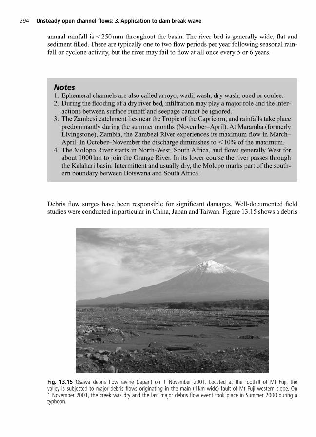
annual rainfall is �250 mm throughout the basin. The river bed is generally wide, flat andsediment filled. There are typically one to two flow periods per year following seasonal rain-fall or cyclone activity, but the river may fail to flow at all once every 5 or 6 years.

294 Unsteady open channel flows: 3. Application to dam break wave

Notes1. Ephemeral channels are also called arroyo, wadi, wash, dry wash, oued or coulee.2. During the flooding of a dry river bed, infiltration may play a major role and the inter-

actions between surface runoff and seepage cannot be ignored.3. The Zambesi catchment lies near the Tropic of the Capricorn, and rainfalls take place

predominantly during the summer months (November–April). At Maramba (formerlyLivingstone), Zambia, the Zambezi River experiences its maximum flow in March–April. In October–November the discharge diminishes to �10% of the maximum.

4. The Molopo River starts in North-West, South Africa, and flows generally West forabout 1000 km to join the Orange River. In its lower course the river passes throughthe Kalahari basin. Intermittent and usually dry, the Molopo marks part of the south-ern boundary between Botswana and South Africa.

Debris flow surges have been responsible for significant damages. Well-documented fieldstudies were conducted in particular in China, Japan and Taiwan. Figure 13.15 shows a debris

Fig. 13.15 Osawa debris flow ravine (Japan) on 1 November 2001. Located at the foothill of Mt Fuji, thevalley is subjected to major debris flows originating in the main (1 km wide) fault of Mt Fuji western slope. On1 November 2001, the creek was dry and the last major debris flow event took place in Summer 2000 during atyphoon.

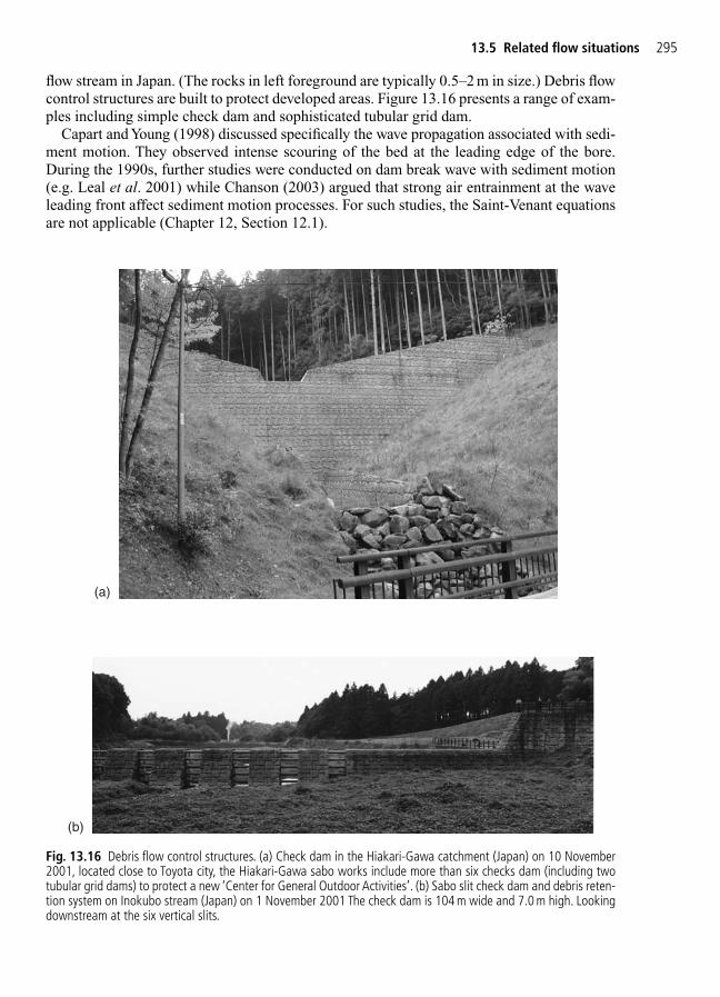
flow stream in Japan. (The rocks in left foreground are typically 0.5–2 m in size.) Debris flowcontrol structures are built to protect developed areas. Figure 13.16 presents a range of exam-ples including simple check dam and sophisticated tubular grid dam.

Capart and Young (1998) discussed specifically the wave propagation associated with sedi-ment motion. They observed intense scouring of the bed at the leading edge of the bore.During the 1990s, further studies were conducted on dam break wave with sediment motion(e.g. Leal et al. 2001) while Chanson (2003) argued that strong air entrainment at the waveleading front affect sediment motion processes. For such studies, the Saint-Venant equationsare not applicable (Chapter 12, Section 12.1).

13.5 Related flow situations 295

(a)

(b)

Fig. 13.16 Debris flow control structures. (a) Check dam in the Hiakari-Gawa catchment (Japan) on 10 November2001, located close to Toyota city, the Hiakari-Gawa sabo works include more than six checks dam (including twotubular grid dams) to protect a new ‘Center for General Outdoor Activities’. (b) Sabo slit check dam and debris reten-tion system on Inokubo stream (Japan) on 1 November 2001 The check dam is 104 m wide and 7.0 m high. Lookingdownstream at the six vertical slits.

A related form of dam break wave is the wave runup in the swash zone. On the beach slope,waves run up after breaking like positive surges (Fig. 13.17). Figure 13.17 shows two examplesof positive surges advancing against the gentle sandy slope. Note the significant amount ofair bubble entrainment in the wave front (i.e. ‘white waters’) (Fig. 13.17(a)). Often the surgepropagation takes place over retreating waters: i.e. against water run down. The swash zonewave runup is believed to be a significant factor in sediment processes in coastal zones (e.g. Longo et al. 2002, Elfrink and Baldock 2002).

296 Unsteady open channel flows: 3. Application to dam break wave

(c)

Fig. 13.16 (Contd ) (c) Tubular grid dam on the Furan River (Japan) in 2002 (courtesy of Dr Marie Augendre and Prof. Okada).

Notes1. Debris comprise mainly large boulders, rock fragments, gravel-sized to clay-sized

material, tree and wood material that accumulate in creeks. The term debris flow isvery broad. In its broad sense, it includes granular flows (and rockslides), mud flows(and paste flows) and wooden debris.

2. The Japanese word sabo means mountain protection system.

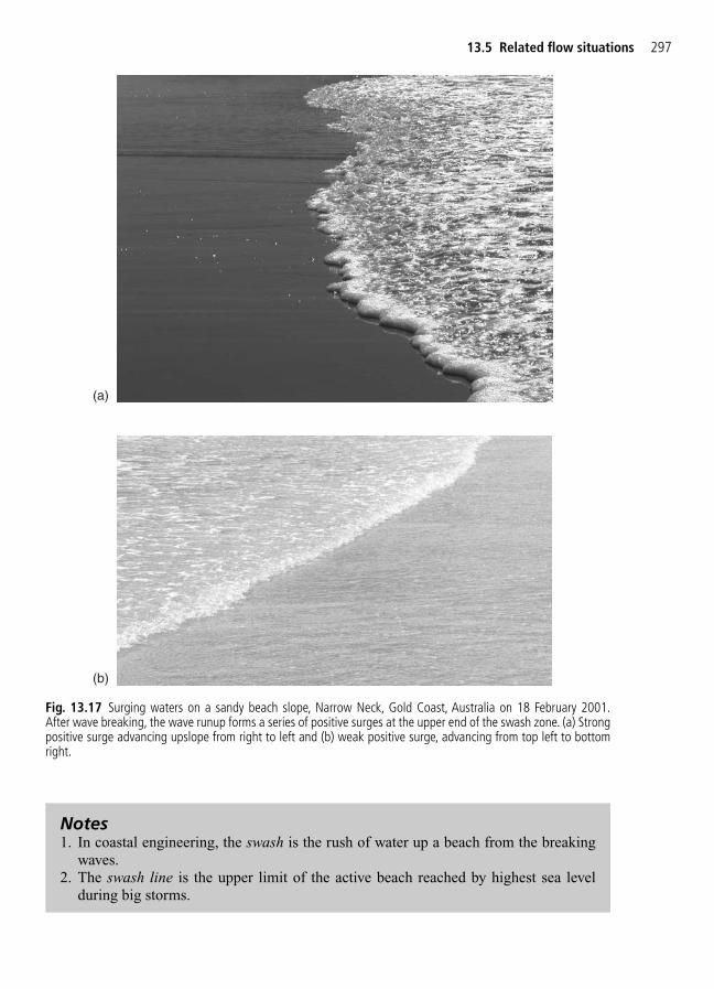
13.5 Related flow situations 297

(a)

(b)

Fig. 13.17 Surging waters on a sandy beach slope, Narrow Neck, Gold Coast, Australia on 18 February 2001.After wave breaking, the wave runup forms a series of positive surges at the upper end of the swash zone. (a) Strongpositive surge advancing upslope from right to left and (b) weak positive surge, advancing from top left to bottomright.

Notes1. In coastal engineering, the swash is the rush of water up a beach from the breaking

waves.2. The swash line is the upper limit of the active beach reached by highest sea level

during big storms.

A tsunami is a long-period wave generated by ocean bottom motion during an earthquake.Occasionally it might be caused by another earth movement (e.g. underwater landslide, vol-canic activity). The wave length is typically about 200–350 km and the tsunami behaves as ashallow-water wave, even in deep sea. Although the wave amplitude is moderate in the mid-dle of the ocean (e.g. 0.5–1 m), the tsunami wave slows down and the wave height increases

298 Unsteady open channel flows: 3. Application to dam break wave

Fig. 13.18 America (Peruvian Warship) beached and partially dismasted at Arica, Chile, following the 13 August1868 tidal wave that washed her and other vessels ashore, photographed from the seaward side. The ship in the dis-tance, beyond America’s bow, is USS Wateree (courtesy of US Naval Historical Center, photograph NH 496 receivedfrom Captain Dudley W. Knox in 1934).

Fig. 13.19 Tsunami warning road sign post off Takatoyo Beach (Enshu Coast, Japan) on 27 March 1999).Note the drawings of surfers and fishermen.

near the shoreline, with periods ranging between 20 min and several hours typically. Thewave runup height might reach several metres above the natural sea level. Major tsunami dis-asters were associated with well in excess of 140 000 losses of life (e.g. Yeh et al. 1996,Hebenstreit 1997, Chanson et al. 2000).

The tsunami wave runup may be a slow rise of water level or an advancing bore. The boremay be a surging bore resulting from the advance of an undular surge wave or a breakingwave associated with load noises. Visual observation suggest that the runup is a turbulentprocess characterized by significant scouring and sediment transport. When the coastline isflat, the abnormal rise of sea level associated with the tsunami wave may runup across flatlands, sweeping away buildings and carrying ships inland (e.g. Figs 13.18 and 13.19).

13.6 Exercises

1. A 15 m high dam fails suddenly. The dam reservoir had a 13.5 m depth of water and thedownstream channel was dry. (1) Calculate the wave front celerity, and the water depth atthe origin. (2) Calculate the free-surface profile 2 min after failure. Assume an infinitelylong reservoir and use a simple-wave analysis (So � Sf � 0).

2. A vertical sluice shut a trapezoidal channel (3 m bottom width, 1V:3H side slopes). The waterdepth was 4.2 m upstream of the gate and zero downstream (i.e. dry channel). The gate issuddenly removed. Calculate the negative wave celerity. Assuming an ideal dam break wave,compute the wave front celerity and the free-surface profile 1 min after gate removal.

3. A 5 m high spillway gate fails suddenly. The water depth upstream of the gate was 4.5 mdepth and the downstream concrete channel was dry and horizontal. (1) Calculate thewave front location and velocity at t � 3 min. (2) Compute the discharge per unit width at the gate at t � 3 min. Use Dressler’s theory assuming f � 0.01 for new concrete lining.(3) Calculate the wave front celerity at t � 3 min using Whitham’s theory.

4. A horizontal, rectangular canal is shut by a vertical sluice. There is no flow motion oneither side of the gate. The water depth is 3.2 m upstream of the gate and 1.2 m downstream.The gate is suddenly lifted. (1) Calculate the wave front celerity, and the surge frontheight. (2) Compute the water depth at the gate. Is it a function of time?

13.6 Exercises 299

Notes1. Tsunami is a Japanese word meaning ‘harbour wave’. A tsunami is also called seis-

mic sea wave. It is sometimes incorrectly termed ‘tidal wave’ but the process is notrelated to the tides.

2. One of the most devastating tsunami catastrophe occurred on 15 June 1896 along theSanriku Coast which destroyed most of Yoshihama and Kamaishi townships (Japan).More than 26 000 people perished. Tsunami warning signs are often seen in Japancoastal zones (e.g. Fig. 13.19).

3. During the tsunami on 8 August 1868 in Peru and Northern Chile, the USS Watereeand the Peruvian warship America were carried about 1 km inland (Fig. 13.18).

4. A related case is the impulse wave generated by rockfalls, landslides, ice falls, glacierbreakup or snow avalanches in lakes and man-made reservoirs. Some impulse wavesmight be induced by earthquake-generated falls. Vischer and Hager (1998) gave athorough summary of the hydraulics of impulse waves.

5. The 40 m high Zayzoun Dam failed on Tuesday 4 June 2002. The dam impounded a 35 mdepth of water and failed suddenly. The depth of water in the downstream channel was0.5 m. (1) Estimate the free-surface profile 7 min after the failure. (2) Calculate the time atwhich the wave will reach a point 10 km downstream of the dam and the surge frontheight. Assume an infinitely long reservoir and a horizontal, smooth channel and use asimple-wave analysis (So � Sf � 0).

6. A narrow valley is closed by a tall arch dam. The average bed slope is 0.08 and the valleycross-section is about rectangular (25 m width). At full reservoir level, the water depthimmediately upstream of the dam is 42 m. In a dam break wave situation, (a) predict thewave front propagation up to 45 km downstream of the dam and (b) calculate the wavefront celerity and depth as it reaches a location 25 km downstream of the dam site. UseHunt’s theory assuming f � 0.06.

7. The Cercey reservoir is a an artificial water supply reservoir held by a 18-m high embank-ment. A breach develops in the embankment. In first approximation, the reservoir level maybe assumed constant. Estimate the breach characteristics 3 min after failure. Calculate thebreach hydrograph for the first 15 min after overtopping. Assume a cohesionless embankment.Notes: Completed in 1836, the Cercey Reservoir (France) is part of the water supply of theBurgundy canal. The earthfill embankment was subjected to several slips prior to 1842.The embankment height is 14 m and its length is 1 km.

8. A 32 m high embankment dam is overtopped and fails rapidly. Estimate the breach char-acteristics for the first 20 min after failure, including the outflow volume. Assume an infi-nitely long reservoir and cohesionless embankment.

13.7 Exercise solutions

1. U � 23 m/s, d(x � 0) � 6 m.2. The assumption of hydrostatic pressure distribution is valid for t � 3 �do / g

—––~ 2 s. Hence

the Saint-Venant equations may be applied for t � 60 s. Note the non-rectangular channelcross-section. For a trapezoidal channel, the celerity of a small disturbance is:

where W is the bottom width and is the angle with the horizontal (i.e. cot � 3).The method of characteristics predicts that the celerity of the negative wave is: �Co �

�4.7 m/s. The celerity of the wave front is U � 2 � Co � 9.6 m/s. Considering a backwardcharacteristics issuing from the dam break wave front, the inverse slope of the C2 character-istics is a constant:

The integration gives the free-surface profile equation at a given time t:

xt

gd W dW d

gd W dW d

2 ( cot 2 cot

3( cot

2 coto o

o

� �

��

) )

dd

2 3oxt

V C C C� � � �

C gAB

gd W dW d

( cot

2 cot� �

)

300 Unsteady open channel flows: 3. Application to dam break wave

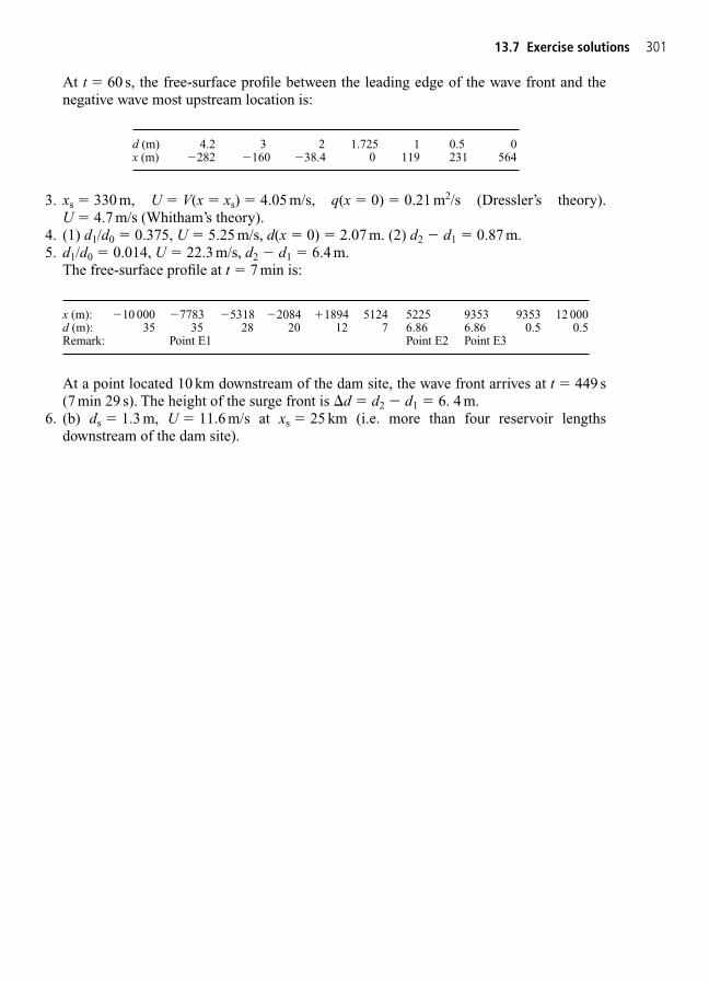
At t � 60 s, the free-surface profile between the leading edge of the wave front and thenegative wave most upstream location is:

d (m) 4.2 3 2 1.725 1 0.5 0x (m) �282 �160 �38.4 0 119 231 564

3. xs � 330 m, U � V(x � xs) � 4.05 m/s, q(x � 0) � 0.21 m2/s (Dressler’s theory).U � 4.7 m/s (Whitham’s theory).

4. (1) d1/d0 � 0.375, U � 5.25 m/s, d(x � 0) � 2.07 m. (2) d2 � d1 � 0.87 m.5. d1/d0 � 0.014, U � 22.3 m/s, d2 � d1 � 6.4 m.

The free-surface profile at t � 7 min is:

x (m): �10 000 �7783 �5318 �2084 1894 5124 5225 9353 9353 12 000d (m): 35 35 28 20 12 7 6.86 6.86 0.5 0.5Remark: Point E1 Point E2 Point E3

At a point located 10 km downstream of the dam site, the wave front arrives at t � 449 s(7 min 29 s). The height of the surge front is �d � d2 � d1 � 6. 4 m.

6. (b) ds � 1.3 m, U � 11.6 m/s at xs � 25 km (i.e. more than four reservoir lengths downstream of the dam site).

13.7 Exercise solutions 301

14

Numerical modelling of unsteadyopen channel flows

SummaryThe numerical modelling of unsteady open channel flows is described. Thedevelopment is based upon the Saint-Venant equations and the method of characteristics. Simple examples of explicit and implicit methods arepresented.

14.1 Introduction

This chapter deals with the numerical integration of the Saint-Venant equations and the solutions of unsteady open channel flows. The Saint-Venant equations were developed forone-dimensional flows, hydrostatic pressure distributions, small bed slopes, constant waterdensity and assuming that the flow resistance is the same as for a steady uniform flow for thesame depth and velocity. The differential form of the equations is:

(14.1)

(14.2)

where A is the flow cross-section, Q is the flow rate, V is the flow velocity, g is the gravityacceleration, So is the bed slope and Sf is the friction slope (Chapter 11).

It is nearly impossible to achieve an exact solution of the Saint-Venant equations, or of thecharacteristic system of equations, because of the non-linear terms V(∂V/∂x) and Sf, andbecause of the complexity of several functions: e.g. A(d), B(d). As a result, a numerical inte-gration is required.

The basic form of the characteristic system of equations is:

(14.3a)DD

2 ) ( Forward characteristicsf otV C g S S( ) � � �

∂∂

∂∂

∂∂

Qt x

V A gAdx

gA S S ) ( Momentum equation2o f � �( )

∂∂

∂∂

At

Qx

0 Continuity equation �

14.1 Introduction 303

(14.3b)

along respectively:

(14.4a)

(14.4b)

Considering the characteristics C1 and C2 through the points D1 and D2 (Fig. 14.1), thecharacteristic trajectories intersect at point E1 (Fig. 14.1). The integration of the characteris-tic system of equations gives:

(14.5a)

(14.5b)

(14.6a)

(14.6b)

If the initial conditions at points D1 and D2 are known, equations (14.5a), (14.5b), (14.6a)and (14.6b) form a system of four equations with four unknowns: xE1, tE1, dE1 and VE1. Theyare exact but non-linear equations because:

C gAB

A A d B B d Sf VgdE1

E1

E1E1 E1 E1 E1 f

E1 E12

E1

( ( 8

for a wide channelE1

� � �) ) �

x x V C tt

tE1 D2 ( )d Backward characteristics C2

D2

E1� �∫

x x V C tt

tE1 D1 ( )d Forward characteristics C1

D1

E1� ∫

V C V C g S S tt

tE1 E1 D2 D2 f o 2 2 ( d Backward characteristics

D2

E1� � � � � )∫

V C V C g S S tt

tE1 E1 D1 D1 f o 2 2 ( d Forward characteristics

D1

E1 � � � )∫

dd

Backward characteristics C2xt

V C� �

dd

Forward characteristics C1xt

V C�

DD

2 ) ( Backward characteristicsf otV C g S S( )� � � �

t

x

�x

�t

D1 D2

E1

Backwardcharacteristic

Forwardcharacteristic

Fig. 14.1 Sketch of the characteristic trajectories.

304 Numerical modelling of unsteady open channel flows

A first approximation consists in performing a trapezoidal integration of the characteristicsystem of equations:

(14.7a)

(14.7b)

(14.8a)

(14.8b)

The error on the flow conditions at the point E1 is a function of two parameters: i.e. the errorintroduced by the trapezoidal integration and the number of iterations. It can be shown math-ematically that the accuracy of the numerical integration is greatly enhanced by increasingthe number of iterations and decreasing the distance �x � xD1 � xD2, and that it converges tothe exact solution.

x x t tV V C C

E1 D2 E1 D2E1 D2 E1 D2 (

2

2

� �

�

)

x x t tV V C C

E1 D1 E1 D1E1 D1 E1 D1 (

2

2

� �

)

V C V C g t tS S S S

E1 E1 D2 D2 E1 D2f f o o 2 2 (

2

E1 D2 E1 D2� � � � �

�

)

2

V C V C g t tS S S S

E1 E1 D1 D1 E1 D1f f o o 2 2 (

2

E1 D1 E1 D1 � � �

�

)

2

NoteThe trapezoidal integration is the most accurate method of integration techniquebetween two points without additional points.

Finite differences methodsOne of the most frequently used methods of obtaining approximate solutions of partial dif-ferential equations is the method of finite differences, which consists essentially in replacingeach partial derivative by a ratio of differences between two immediate values:

(14.9)

where �V is the increase in the function V during the time step �t.Although finite difference techniques are simple to program, including with a spreadsheet,

there are a number of difficulties in particular associated with numerical instabilities. Forexample, the following explicit finite difference scheme is unstable:

Unstable scheme (14.10a)

Unstable scheme (14.10b)

where the subscript i and superscript n refer respectively to the x-direction and t-axis (Fig.14.2). The numerical scheme (equation (14.10)) is unstable for any value of �x and �t.

∂∂

Vx

V Vx

in

in

in

���

�

11 1 2

∂∂

Vt

V Vt

in

in

in

��

�

1 1

∂∂Vt

Vt

� �

�

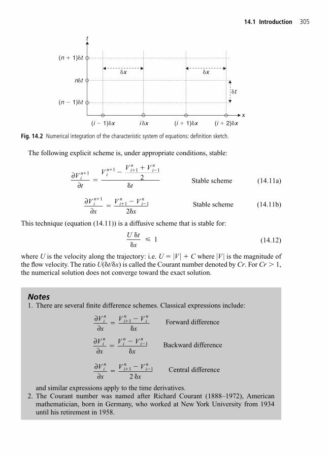
14.1 Introduction 305

The following explicit scheme is, under appropriate conditions, stable:

Stable scheme (14.11a)

Stable scheme (14.11b)

This technique (equation (14.11)) is a diffusive scheme that is stable for:

(14.12)

where U is the velocity along the trajectory: i.e. U � |V | C where |V | is the magnitude ofthe flow velocity. The ratio U(�t/�x) is called the Courant number denoted by Cr. For Cr � 1,the numerical solution does not converge toward the exact solution.

U tx�

�" 1

∂∂

Vx

V Vx

in

in

in

���

�

11 1 2

∂∂

Vt

VV V

tin i

n in

in

�

��

�

11 1 1

2

t

x

�x �x

(i � 1)�x i �x (i 1)�x (i 2)�x

(n � 1)�t

n�t

(n 1)�t

�t

Fig. 14.2 Numerical integration of the characteristic system of equations: definition sketch.

Notes1. There are several finite difference schemes. Classical expressions include:

Forward difference

Backward difference

Central difference

and similar expressions apply to the time derivatives.2. The Courant number was named after Richard Courant (1888–1972), American

mathematician, born in Germany, who worked at New York University from 1934until his retirement in 1958.

∂∂Vx

V Vx

in

in

in

1 1��

� �

2

∂∂Vx

V Vx

in

in

in

1��

��

∂∂Vx

V Vx

in

in

in

1��

�

306 Numerical modelling of unsteady open channel flows

14.2 Explicit finite difference methods

Two well-known explicit finite difference methods are the Lax diffusive scheme and the leap-frog method (Table 14.1, Fig. 14.3) (Liggett and Cunge 1975). Considering the (x, t) planesketched in Fig. 14.2, grid points are identified by the subscript i and by the superscript n to

Table 14.1 Finite difference methods for unsteady open channel flows

Scheme Remarks

(1) (2) (3) (4)

Explicit schemesLax diffusive scheme Stability:

0 " � � 1 and

Leap-frog method Stability:

Implicit schemePreissmann–Cunge Stability:scheme 0.5 " � " 1

V VV V

t

in

in i

nin

�� �

�

1 1 1 (1 )

� �2

V V

xin

in

��

�1 1 2

�

�"

t V C

x

(| | ) 1

V V

tin

in ��

�

1 1 2

V V

xin

in

��

�1 1 2 �

�"

t V C

x

(| | ) 1

12

V V

t

V V

tin

in

in

in

�

�

�

�11

11

�

�

V V

x

V V

x

in

in

in

in

�

�

��

�

11 1

1

(1 )

t

x

�x

(i � 1)�x i �x (i 1)�x

(n 1)�t

n �t

�t

Lax diffusive scheme

∂t

∂x

t

x

�x �x

(i � 1)�x i �x (i 1)�x

(n 1)�t

(n � 1)�t

n �t

�t

�t

Leap-frog scheme

∂V

∂V

∂t

∂x

∂V

∂V

(a)

(b)

Fig. 14.3 Sketch of explicit finite difference schemes: (a) Lax diffusive scheme and (b) leap-frog scheme.

∂∂

V

tin1 ∂

∂V

xin1

14.2 Explicit finite difference methods 307

14.2.1 Lax diffusive method

The continuity and momentum equations (14.1) and (14.2) may be rewritten in terms of theflow rate and free-surface elevation:

Continuity equation (14.13)

Dynamic equation (14.14)

where the friction slope Sf equals:

The Lax diffusive scheme is shown in Table 14.1. It is similar to equation (14.11), with thedifference of a coefficient � satisfying 0 " � � 1. For � � 0, the Lax method equals equa-tion (14.11) which is sometimes called a diffusive scheme. For � � 1, the Lax method isunstable (equation (14.10)). Using the Lax diffusive scheme, the discretization of the con-tinuity and dynamic equations yields:

Continuity equation (14.15)

Y YY Y

t BQ Q

x

in

in i

nin

in

in

�

�

� �

�

�

��

1 1 1

1 1

(1

1

2 0

� �)2

SQ Qgf

ADf

2 H

|�

|8

4

∂∂

∂∂

∂∂

Qt x

QA

gAYx

gAS 02

f �

∂∂

∂∂

Yt B

Qx

1

0 �

DiscussionThe numerical integration of the characteristic system of equations does not require con-stant, uniform spatial and time steps. In a general case, Vn

i becomes the discrete value ofthe velocity at a distance x from left boundary and a time t from the origin that satisfy:

NoteThe term ‘explicit’ implies that the flow properties at x � x1 � 0 and t � t1 � 0 can becalculated as functions of the flow conditions at t � t1 and that they are independent ofthe flow properties for t � t1.

t tkk

n

1

� ��∑

x x jj

i

1

� ��∑

indicate spatial intervals and time steps respectively. For example, Vni is the discrete value of

the flow velocity at a distance x � i�x from the left boundary where x � 0 and i � 0, and attime t � n�t from the initial conditions where t � 0 and n � 0, assuming constant spatial andtime intervals �x and �t.

308 Numerical modelling of unsteady open channel flows

(14.16)

In the continuity equation, the term B is not explicitly defined. A simple assumption is:B � Bn

i. Similarly the terms A and Sf in the dynamic equation (14.16) may be assumed to beequal to An

i and Sfni respectively.

The continuity and dynamic equations form a system of two equations with two unknownsYi

n1 and Qin1. It may be solved explicitly:

(14.17)

(14.18)

The Lax diffusive method is characterized by some numerical diffusion for � � 0 thatintroduces numerical inaccuracies. At the limit, for a steady flow, the Lax diffusive schemepredicts a horizontal free surface which is untrue. Basically the method is stable numericallyfor � � 1 and:

(14.19)

Practically equation (14.19) imposes an upper limit to the time step �t. For example, consider-ing a large river with a mean water depth of 2 m and mean velocity of 1 m/s, the time step �tmust satisfy: �t " �x/4.4. If the spatial interval �x equals 1 km, the time step must be less than226 s. A natural flood in such a river system is likely to spread over several days, possibly fewweeks, and complete unsteady flow calculations may require several thousand iterations.

�

�"

t V Cx

(| | ) 1

Q QQ Q t

xQA

QA

tx

gA Y Y t gA

in

in i

nin

i

n

i

n

in

in

in

i

�

�

�

� �

��

��

��

�� � �

1 1 12

1

2

1

1 1

(1 )

2

2

(

� �2

) nni

nSf

Y YY Y t

B

Q Qxi

nin i

nin

in

in

in

� �� $ � $

� �

�1 1 1 1 1 (1 )

2

2

Q QQ Q

t

QA

QA

x

gAY Y

xAS

in

in i

nin

i

n

i

n

in

in

�

�

�

� �

�

�

�

�

� �

1 1 12

1

2

1

1 1f

(1 )

2

2

g 0 Dynamic equation

� �2

Notes1. The continuity and momentum equations (14.1) and (14.2) are:

Continuity equation (14.1)

Momentum equation (14.2)∂∂

∂∂

∂∂

Qt x

V A gAdx

gA S S ) ( 2o f � �( )

∂∂

∂∂

At

Qx

0 �

14.2 Explicit finite difference methods 309

Boundary conditionsThe free-surface elevation Yi

n1 can be computed, using equation (14.17), at the time stept � (n 1)�t and at the locations x � i�x for i � 1, 2, …, N � 1, but at the boundaries (i.e.Y0

n1 and Y Nn1). Equation (14.18) allows the computations of the flow rate Qi

n1 at the timet � (n 1)�t and at the locations x � i�x for i � 1, 2, …, N � 1, but at the boundaries (i.e.Q0

n1 and QNn1).

The implementation of boundary conditions has been discussed in Chapter 11 (Section11.3.2 and Table 11.1). Basically, for a limited reach with subcritical flow conditions, oneflow condition must be prescribed at each boundary for t � 0. In supercritical flows, two flowproperties are required at the upstream boundary.

Considering the left boundary sketched in Fig. 14.4, at the time step t � n�t, the flow con-ditions at the previous time step are known: i.e. Yn

0 and Qn0, Y

n1 and Qn

1. One boundary condi-tion may be deduced from the method of characteristics. For the subcritical flow sketched inFig. 14.4, the equations of the characteristics C2 through the left boundary give:

Backward characteristics (14.5b)

Backward characteristics C2 (14.6b)

where the point S is located at the intersection of the backward characteristics with the timestep t � n�t and assuming xi�0 � 0 at the left boundary. Equations (14.5b) and (14.6b) forma system of two equations with two unknowns V n1

i�0 and xS (or Q n1i�0 and xs). A similar

reasoning may be conducted at the right boundary (i � N) using a forward characteristic trajectory.

This treatment of the boundary conditions is not specific to the Lax diffusive method. It isgeneral to all explicit schemes including the leap-frog method (Section 14.2.2).

x x V C ti n t

n t� �

�� � �0 S

( 1) ( ) d 0∫

( )V C V C g S S tin

in

n t

n t�

�

�

�� � � � �0

101

S S f( 1)

o 2) 2 ( d∫

They may be rewritten in terms of the discharge Q and free-surface elevation Y as:

Continuity equation (14.13)

Dynamic equation (14.14)

where

2. The momentum equation (14.2) is commonly called the dynamic equation.3. The Lax diffusive scheme was advocated by J.J. Stoker although it is often attributed

to J. Keller and P. Lax (Montes 1998, p. 502). Isaacson et al. (1958) developed an ini-tial discretization scheme assuming � � 0.5 while Liggett and Cunge (1975) detailedthe present scheme commonly called Lax diffusive scheme.

SQ Q

gf

ADf

2 H

| |�

84

∂∂

∂∂

∂∂

Qt x

QA

gAYx

gAS 02

f �

∂∂

∂∂

Yt B

Qx

1

0 �

310 Numerical modelling of unsteady open channel flows

ApplicationDevelop the characteristic equations for subcritical flows.

Solution (1): Left boundaryConsidering the left boundary sketched in Fig. 14.4, the equations of the characteristicsC2 through the left boundary give:

(14.5b)

(14.6b)

The flow properties at the point S may be interpolated with those at adjacent points atthe same time level: i.e. points A and B in Fig. 14.4. With linear interpolations, thevelocity V and celerity C are determined as:

Using the parabolic procedure, it yields:

Vx x

xV V V x x

xV V V

Vn n n n n n

nS

S 0 0 1 2 S 0 0 1 20

2 2

3 4

2 �

�

�

�

�

�

� �

2

Cx x

xC C Cn n n

SS 0

1 0 0

( ��

�� )

Vx x

xV V Vn n n

SS 0

1 0 0

( ��

�� )

x x V C tn t

n t0 S

( 1) ) d 0� � �

�

�(∫

( )V C V C g S S tn nn t

n t0

10

1S S f o

( 1) 2) 2 ( d

�

�� � � � �∫

t

x

�x �x

(n 1)�t

n �t

�t

Left boundary condition

i � 1 i � 2i � 0

C2

A BS

t

x

�x �x

(n 1)�t

n �t

�t

Right boundary condition

i � N – 1 i � Ni � N – 2

C1

SR T

Fig. 14.4 Boundary conditions.

14.2 Explicit finite difference methods 311

14.2.2 Leap-frog scheme

The leap-frog method uses centred differences for time and space (Table 14.1, Fig. 14.3(b)).The discretization of the continuity and dynamic equations yields:

Continuity equation (14.20)

Dynamic equation (14.21)

The continuity and dynamic equations form a system of two equations which may be solvedexplicitly:

(14.22)

(14.23)

Q Qtx

QA

QA

tx

gA Y Y

t gA S

in

in

i

n

i

n

in

in

in

in

in

�

�

�� ��

�� �

�

��

� �

1 12

1

2

1

1 1

f

(

2

)

Y Ytx B

Q Qin

in

in i

nin �

�� �

��1 1

1 1 1

( )

Q Qt

QA A

x

gAY Y

xgA S

in

in

i

n

i

n

in i

nin

in

in

� �

�

�

�

�

�

�

� �

1 11

2

1

1 1f

Q

2

2

0

2

2

Y Yt B

Q Qx

in

in

in

in

in �

��

�

�

��

1 11 1

1

2 0

2

The parabolic interpolation is more precise than the linear one.Altogether this gives a system of four equations with four unknowns xS, VS, CS and

Vn10 (or Qn1

0 ).

Solution (2): Right boundaryConsidering the right boundary sketched in Fig. 14.4, the equations of the characteris-tics C1 give:

(14.5a)

(14.6a)

Using a linear interpolation between points R and T (Fig. 14.4), the flow properties atthe point S are:

Cx x

xC C CN

Nn

Nn

Nn

SS 1

1 1

( ��

�� �

� �)

Vx x

xV V VN

Nn

Nn

Nn

SS 1

1 1

( ��

�� �

� �)

x x V C tN n t

n t ( )d 0S

( 1) � �

�

�

∫

V C V C g S S tNn

Nn

n t

n t

�

� � � �1 1

S S f o( 1)

2 2 ( d)∫

Cx x

xC C C x x

xC C C

Cn n n n n n

nS

S 0 0 1 2 S 0 0 1 20

2 2

3 4

2 �

�

�

�

�

�

� �

2

312 Numerical modelling of unsteady open channel flows

Equations (14.22) and (14.23) give the free-surface elevation Yin1 and flow rate Qi

n1 at the(n 1) time step for i � 1, 2, …, N � 1, but at the boundaries (i.e. i � 0 and N).

The leap-frog scheme is stable for:

(14.19)�

�"

t V Cx

(| | ) 1

Notes1. The leap-frog scheme is called ‘schéma en quinconce’ in French. It is one of the earli-

est numerical schemes and was used by Lewis Fry Richardson in his 1910 paper onstress calculation in masonry dams (Montes 1998, p. 509).

2. Lewis Fry Richardson (1881–1953) was a British meteorologist. He pioneered math-ematical weather forecasting. He made contributions to the theory of calculus and thestudy of diffusion.

3. Note that the calculations of free-surface elevation Yin1 and flow rate Qi

n1 arebasically independent of Yi

n and Qin (Fig. 14.3(b)). Basically the points in the (x, t)

space form two independent grids. This may result in saw-tooth distributions of flowrate and free-surface elevation.

14.2.3 Discussion

Practically the leap-frog scheme introduces less numerical errors than the Lax diffusivemethod. The leap-frog scheme is of second order rather than first order, and it is non-dissipative.There is no numerical diffusion terms like in the Lax diffusive method. Liggett and Cunge(1975) added on the leap-frog method: ‘mass conservation […] is very good because theapproximation of the continuity equation is of second order for B � constant. Unfortunatelythe solution obtained is a saw-tooth line since the points where the dependent variables arecomputed are alternately odd or even’ (p. 121).

14.3 Implicit finite difference methods

Explicit schemes are very simple and they are well suited for interior grid points. Two majordisadvantages are the treatment of the boundary conditions and the stability criterion (equa-tion (14.19)). Modern numerical models of unsteady open channel flows are based uponsome implicit finite difference methods.

The most common implicit method for unsteady open channel flows is the Preissmann–Cunge scheme (Fig. 14.5). The dependent variables and their derivatives are discretized as:

(14.24)

(14.25)∂∂

Vt

V Vt

V Vt

in

in

in

in

in

��

�

�

�

111

11

12

V V V V Vin

in

in

in

1 1

1 11�

�

� �

2 2( ) ( )

14.3 Implicit finite difference methods 313

(14.26)

where � is a weighting parameter. It can be shown that unconditional stability occurs only inthe range:

The discretization of the continuity and dynamic equations yields:

Continuity equation (14.27)

12

2 2 2 2

Q Qt

Q Qt

QA

QA

x

QA

QA

x

in

in

in

in

i

n

i

n

i

n

i

n

�

�

�

�

�

� �

�

�

11

11

1

1 1

1

(1 )

� �

( ) ( )

�

�

� �

�

�

1

(1 )

11 1

111 1

1g A A A AY Y

xY Y

x

g A

in

in

in

in i

nin

in

in

i

� �� �

�

2 2

2 111 1

1

f 11

f1

f 1 f

1

1

0 Dynamic equation

nin

in

in

in

in

in

in

A A A

S S S S

�

� �

�

( ) ( )

�

� �

2

2 2

12

2 2

Y Yt

Y Yt

Q Qx

Q Qx

B B B

in

in

in

in

in

in

in

in

in

in

in

�

�

�

�

�

� �

�

�

�

11

11

11 1

1

11 1

1

(1 )

1

( )� �

� �BBi

n( ) 0�

0 5. 1� ��

∂∂

Vx

V Vx

V Vx

in

in

in

in

in

��

� �

�

�

111 1

1

(1

� �)

t

x�x

i �x (i 1)�x

(n 1)�t

n �t

�t

Preissmann–Cunge scheme

0.5 0.5

1– u

u

Fig. 14.5 Sketch of the Preissmann–Cunge implicit finite difference scheme.

(14.28)

314 Numerical modelling of unsteady open channel flows

Note that any function of water depth, e.g. the free-surface width B, satisfies:

Considering a river reach (i � 0, 1, …, N), there are 2(N 1) unknowns at the time step(n 1) while equations (14.27) and (14.28) provide 2N equations between two adjacentpoints {i} and {i � 1}. Including the two boundaries conditions at i � 0 and N, it yields asystem of 2N 2 equations with 2(N 1) unknowns.

B BBd

d dBY

Y Yin

in

i

n

in

in

i

n

in

in � � � � �1 1 1 ( (

∂∂

∂∂

) )

Notes1. In an ‘implicit’ scheme, the flow properties must be calculated simultaneously at once.

For example, this may be achieved by a matrix inversion operation. In other words,the flow properties at x � x1 � 0 and t � t1 � 0 are functions of the flow conditionsat t � t2 � t1.

2. The Preissmann–Cunge method was first developed in 1960 and extended in the fol-lowing years (Preissmann 1960, Preissmann and Cunge 1961, Cunge and Berthier1962, Cunge and Wegner 1964).

3. The Preissmann–Cunge scheme is also called the four-point implicit method, boxmodel, Preissmann implicit scheme or Sogreah implicit method.

4. Alexandre Preissmann (1916–1990) was born and educated in Switzerland. From1958, he worked on the development of mathematical models at Sogreah in Grenoble.

5. Born and educated in Poland, Jean A. Cunge worked in France at Sogreah inGrenoble and he lectured at the Hydraulics and Mechanical Engineering School ofGrenoble (ENSHMG).

DiscussionThe Preissmann–Cunge method is an implicit scheme. Although more complicated than theexplicit methods, its major advantages include the stability of the scheme, the computationof discontinuities (e.g. hydraulic jump), the calculations of the boundary conditions and thevariable spatial interval �x.

The Preissmann–Cunge scheme is unconditionally stable for 0.5 " � " 1: i.e. the stabilityis neither a function of the time step nor Courant number. Practically Liggett and Cunge(1975) recommended to select a weighting parameter satisfying:

For � � 0.5, the scheme is always unstable while parasite oscillations were found for0.5 " � � 0.66 (Liggett and Cunge 1975, p. 163). Further studies suggested an optimumvalue � for 0.6 " � " 0.75.

The boundary conditions (i.e. i � 0 and N) may be introduced simply. For example, if thefree-surface elevation Y(t) is a known function of the time at the left boundary, this gives thefollowing additional relationships:

Boundary conditionY f tnn0

11 (

� )

0 6. 1" "�

14.4 Exercises 315

If the discharge is a known function of time at the right boundary, it gives:

Boundary condition

If the discharge is a known function of the free-surface elevation time at the right bound-ary, this gives:

Boundary condition

where df/dY is the derivative of the stage–discharge relationship at the boundary.In the Preissmann–Cunge scheme (equations (14.27) and (14.28)), only the locations {i}

and {i 1} are linked: i.e. over one spatial interval �x (Fig. 14.5). As a result, it is possibleto change the longitudinal increment �x without affecting the stability nor accuracy of theresults.

Cunge (1975) showed that hydraulic discontinuities can be calculated using a variableweighting factor � in the Preissmann–Cunge method.

Q QQY

Y YfY

Y YNn

Nn

N

n

Nn

Nn

N

n

Nn

Nn � � � � �1 1 1 ( )

dd

( ∂∂

)

Q f YNn

Nn �1 1 ( )

∂∂

( )Q

YY Y Q Q f t f t

N

n

Nn

Nn

Nn

Nn

n n

� � � � �1 11 ( () )

Q f tNn

n

�11 ( )

� � � � �Y Y Y f t f tn n n

n n0 01

0 1 ( () )

NoteAlthough the stability of the Preissmann–Cunge method is independent of the Courantnumber, the accuracy of the results decreases with increasing Courant number forCr � 1.

14.4 Exercises

1. Why the Saint-Venant equations cannot usually be solved with analytical equations?2. Using a sketch, explain the basic differences between forward, backward and central dif-

ference methods.3. Write the Courant number for a finite difference scheme.4. What are the basic differences between an explicit and implicit numerical scheme?5. Is the Lax diffusive scheme always stable? Detail your answer.6. Is the leap-frog scheme an implicit method? What is(are) the unusual feature(s) of the

leap-frog scheme?7. Is the Preissmann–Cunge scheme an implicit method? For what range of the Courant

number is it stable?

Part 3 Revision exercises

SummaryIn this section, applications of unsteady open channel flows are reviewed.Simple exercises are developed for different types of applications.

Revision exercise no. 1

A long irrigation channel is controlled by a downstream gate. During a gate operation, theflow velocity, immediately upstream of the gate, increases linearly from 0 to 1 m/s in 2 min.Initially the flow is at rest and the water depth is 2 m. Neglecting bed slope and friction slope,calculate the water depths at the gate, at mid-distance and at the canal intake at t � 6 min.Compare the simple wave solution with the Hartree method.

SolutionThe simple wave solution was developed in Chapter 12. Results at t � 6 min are presented inFig. R.3, where the coordinate system is x � 0 at the downstream end and x is positive in theupstream direction.

The simple wave solution is an exact, theoretical solution of the Saint-Venant equations.The Hartree method is only a numerical approximation, and discrepancies between the exactsolution and the numerical integration are seen.

Revision exercise no. 2

The Virdoule River flows in Southern France. It is known for its flash floods associated withextreme rainfall events, locally called ‘épisode cévenol’. These are related to large masses ofair reaching the Cévennes Mountain range. The Virdoule River is about 50 m wide. Initiallythe water depth is 0.5 m and the flow rate is 25 m3/s. During an extreme rainfall event, the dis-charge at Quissac increases from 25 to 1200 m3/s in 6 h. (Assume a linear increase of flowrate with time.) The flow rate remains at 1200 m3/s for an hour and then decreases down to400 m3/s in the following 12 h:

(a) Compute the celerity of the monoclinal wave for the flash flood (i.e. increase in flow ratefrom 25 to 1200 m3/s). Assume uniform equilibrium flows and So � 0.001.

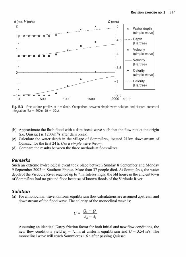
Revision exercise no. 2 317

(b) Approximate the flash flood with a dam break wave such that the flow rate at the origin(i.e. Quissac) is 1200 m3/s after dam break.

(c) Calculate the water depth in the village of Sommières, located 21 km downstream ofQuissac, for the first 24 h. Use a simple wave theory.

(d) Compare the results between the three methods at Sommières.

RemarksSuch an extreme hydrological event took place between Sunday 8 September and Monday 9 September 2002 in Southern France. More than 37 people died. At Sommières, the waterdepth of the Virdoule River reached up to 7 m. Interestingly, the old house in the ancient townof Sommières had no ground floor because of known floods of the Virdoule River.

Solution(a) For a monoclinal wave, uniform equilibrium flow calculations are assumed upstream and

downstream of the flood wave. The celerity of the monoclinal wave is:

Assuming an identical Darcy friction factor for both initial and new flow conditions, thenew flow conditions yield d2 � 7.1 m at uniform equilibrium and U � 3.54 m/s. Themonoclinal wave will reach Sommières 1.6 h after passing Quissac.

UQ QA A

2 1

2 1

��

�

0 500 1000 1500 2000 x (m)

Water depth(simple wave)

Depth(Hartree)

Velocity(simple wave)

Velocity(Hartree)

Celerity(simple wave)

Celerity (Hartree)

d (m), V (m/s) C (m/s)

�1

0

1

2

2.5

3

3.5

4

4.5

5

Fig. R.3 Free-surface profiles at t � 6 min. Comparison between simple wave solution and Hartree numericalintegration (�x � 400 m, �t � 20 s).

318 Part 3 Revision exercises

(b) For a dam break wave, the flow rate at the dam site (x � 0) is 1200 m3/s:

It yields do � 8.74 m. Note that d1/do � 0.057 and it is reasonable to assume critical flowconditions at x � 0. Downstream of the dam, the initial flow conditions are d1 � 0.5 mand V1 � 1 m/s. Complete calculations show that U � 10.66 m/s, d2 � 2.46 m andV2 � C2 � 3.79 m/s.

The positive surge leading to the dam break wave will reach Sommières 33 min afterthe dam break at Quissac and the wave front height will be 1.96 m. The water depth atSommières will remain as d � d2 until t � 1.53 h. Afterwards, the water depth will grad-ually increase. (Ultimately it would reach 3.9 m assuming an infinitely long reservoir.)

(c) For a simple wave analysis, the boundary conditions correspond to the formation of apositive surge between t � 0 and 6 h, and the formation of a negative surge betweent � 7 and 19 h. The forward characteristics are plotted in Fig. R.4. A positive surge willform rapidly downstream of Quissac and the surge front will reach the township ofSommières at about t � 1.3 h.

(d) Discussion: Between the three calculations, the last one (i.e. simple wave calculations)would be the most accurate. Practically, an important result is the arrival time of the flashflood at Sommières. If the flood is detected at Quissac, the travel time between Quissac

Q x d gd W( 0) 827 o o� �

0

5000

10 000

15 000

20 000

25 000

30 000

35 000

0 5000 10 000 15 000 20 000 25 000 30 000

t � 8 h

Virdoule River Simple wave analysis

t(x � 0) � 0t(x � 0) � 0.25 h

t � 0.5 h

t � 1 ht � 2 h

t � 3 h

t � 5 ht � 6 h

t � 7 h

t � 9 h

x (m)

t (s)

Fig. R.4 Forward characteristics curves for Virdoule River flash flood.

Revision exercise no. 3 319

and Sommières is basically the warning time. The simple calculation predicts 1.3 h. Themonoclinal wave calculations predict 1.6 h and the dam break wave theory gives 33 min.Interestingly all the results are of the same order of magnitude.

Revision exercise no. 3

A senior coastal engineer wants to study sediment motion in the swash zone. For 0.5 m highbreaking waves, the resulting swash is somehow similar to a dam break wave running overretreating waters. (1) Assuming an initial reservoir water depth of 0.5 m, an initial water depthd1 � 0.07 m and an initial flow velocity V1 � �0.4 m/s, calculate the surge front celerity andheight. Assume a simple wave (So � Sf � 0). (2) Calculate the bed shear stress immediatelybehind the surge front. The beach is made of fine sand (d50 � 0.3 mm, d90 � 0.8 mm).Assume ks � 2d90 (Chanson 1999, Table 12.2). For sea water, % � 1024 kg/m3 and � � 1.22 �10�3Pa s. (3) Predict the occurrence of bed load motion and sediment suspension. (4) Duringa storm event, breaking waves near the shore may be 3–5 m high. For a 2 m high breakingwave, calculate the surge front height and bed shear stress behind the surge front assumingan initial reservoir water depth of 2 m, an initial water depth d1 � 0.15 m and an initial flowvelocity V1 � �1 m/s.

SolutionSelect a positive x-direction toward the shore. The dam break wave (do � 0.5 m) propagatesin a channel initially filled with water (d1 � 0.045 m) with an opposing flow velocity(V1 � �0.4 m/s). The x coordinate is zero (x � 0) at wave breaking (i.e. pseudo-dam site)and the time origin is taken at the start of wave breaking.

The characteristic system of equation, and the continuity and momentum principles at thewave front must be solved theoretically. The free-surface profile is horizontal between theleading edge of the positive surge (point E3) and the intersection with the C1 forward char-acteristics issuing from the initial negative characteristics. The flow depth d2 and velocity V2behind the surge front satisfy the continuity and momentum equations as well as the condi-tion along the C1 forward characteristics:

Continuity equation

Momentum equation

Forward characteristics

These three equations form a system of three non-linear equations with three unknowns V2,d2 and U. An iterative calculation shows that the surge front celerity is: U/��gd1� � 3.2 andU � 2.12 m/s. At the wave front, the continuity and momentum equations yield:

Hence d2 � 0.21 mdd

U V

gd2

1

1

1

12

1 8

1 4.6� �

� �( )

2

V gd gd2 2 o 2 2 �

d U V d U V gd gd22 2( ) ( )

12

122 1 1 1

222� � � � �

d U V d U V1( ) ( ) 1 2 2� � �

The momentum equation may be rewritten as:

Hence V2 � 1.58 m/s

Behind the surge front, the boundary shear stress equals:

The Shields parameter �* equals 1.55 which is almost one order of magnitude greater than thecritical Shields parameter for bed load motion (�*)c �0.035 (Graf 1971). For a 0.3 mm sandparticle, the settling velocity is 0.034 m/s. The ratio V*/wo equals 2.5 implying sediment suspension (Chanson 1999, Chapter 9, Section 9.2).

For a 2 m high breaking wave during a storm event, the surge front height equals:d2 � d1 � 0.69 m. The boundary shear stress behind the surge front equals: �o � 21 Pa.

Remarks1. The above development has a number of limitations. The reservoir is assumed infinite

although a breaking wave has a finite volume, assuming the beach slope to be frictionlessand horizontal.

2. Note that the calculations of U, V2 and d2 are independent of time.

Revision exercise no. 4

The Qiantang River discharges into the Hangzhou Wan in East China Sea. Between Laoyancangand Jianshan the river is 4 km wide, the bed slope corresponds to a 5 m bed elevation dropover the 50 km reach. At the river mouth (Ganpu, located 30 km downstream of Jianshan), thetidal range at Jianshan is 7 m and the tidal period is 12 h 25 min. At low tide, the river flowsat uniform equilibrium (2.4 m water depth). Discuss the propagation of the tidal bore.

Assume So � Sf, f � 0.015 and a wide rectangular prismatic channel between Laoyancangand Ganpu. (This is an approximation off course. Between Ganpu and Babao (upstream of Jianshan), the channel width contracts from 20 down to 4 km while the channel bed risesgently. The resulting funnel shape amplifies the tide in the estuary.) Sea water density anddynamic viscosity are respectively 1024 kg/m3 and 1.22 �10�3Pa s.

SolutionUniform equilibrium flow calculations are conducted in the Qiantang River at low tide. Ityields: normal velocity � 1.12 m/s (positive in the downstream direction), Co � 4.85 m/s fordo � 2.4 m, f � 0.015 and So � 1 �10�4.

Select a coordinate system with x � 0 at the river mouth (i.e. at Ganpu) and x positive inthe upstream direction. The initial conditions are Vo � �1.12 m/s and Co � 4.85 m/s. Theprescribed boundary condition at the river mouth (Ganpu) is the water depth given as:

where to � t(x � 0) and T is the tide period (T � 44 700 s).

d x tT

t( 0, ) 3.6 72

1 cos2

o� � ��

�

� �o2

8 7.7 Pa� �

fV 2

V

gd

dd

2

2

o

2

2 1 1.1� � �

320 Part 3 Revision exercises

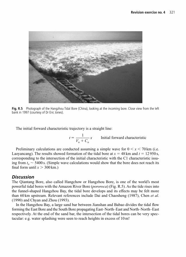
Revision exercise no. 4 321

The initial forward characteristic trajectory is a straight line:

Initial forward characteristic

Preliminary calculations are conducted assuming a simple wave for 0 � x � 70 km (i.e.Laoyancang). The results showed formation of the tidal bore at x � 48 km and t � 12 950 s,corresponding to the intersection of the initial characteristic with the C1 characteristic issu-ing from to � 5400 s. (Simple wave calculations would show that the bore does not reach itsfinal form until x � 300 km.)

DiscussionThe Qiantang Bore, also called Hangchow or Hangzhou Bore, is one of the world’s mostpowerful tidal bores with the Amazon River Bore (pororoca) (Fig. R.5). As the tide rises intothe funnel-shaped Hangzhou Bay, the tidal bore develops and its effects may be felt morethan 60 km upstream. Relevant references include Dai and Chaosheng (1987), Chen et al.(1990) and Chyan and Zhou (1993).

In the Hangzhou Bay, a large sand bar between Jianshan and Babao divides the tidal flowforming the East Bore and the South Bore propagating East–North–East and North–North–Eastrespectively. At the end of the sand bar, the intersection of the tidal bores can be very spec-tacular: e.g. water splashing were seen to reach heights in excess of 10 m!

tV C

x 1

o o

�

Fig. R.5 Photograph of the Hangzhou Tidal Bore (China), looking at the incoming bore. Close view from the leftbank in 1997 (courtesy of Dr Eric Jones).

This page intentionally left blank

PART 4

Interactions between FlowingWater and its Surroundings

Air entrainment at Chinchilla Weir (Australia) in November 1997. Note self-aeration down the chute andthe hydraulic jump in foreground right. The three-phase mixing (air, water and sediment) gave a beigeappearance to the flow.

This page intentionally left blank

15

Interactions between flowingwater and its surroundings:introduction

15.1 Presentation

Open channel hydraulics is possibly the most complicated field in fluid mechanics. First the basic principles form a complex system of non-linear equations (Chapters 2 and 11). Fora given flow rate, there is an infinity of solutions depending upon the bed slope, boundaryfriction and channel cross-sectional shape (e.g. Henderson 1966, Chanson 1999a, 2004b).River flow rates may further range from extreme values: the hydraulics of droughts andfloods are both important for the survival and development of a country. Second there arestrong interactions between the flowing waters and the surrounding environment. This coversthe transport of solids, the dispersion of chemicals, the mixing of air and water at the free sur-faces. Comprehensive reviews include Graf (1971), Rutherford (1994) and Chanson (1997).

Natural channels have the ability to scour channel bed and banks, to carry sediment mater-ials and to deposit sediment load. For example, during a flood event, the Yellow River erodedits bed by 7 m in �60 h at Longmen (Middle reach of Yellow River, July 1966, peak dis-charge: 7460 m3/s) (Wan and Wang 1994). Figure 15.1(a) shows a river in flood. The darkcolour of the waters highlights significant sediment suspension. Figure 15.1(b) and (c) illus-trates intense sediment transport leading to massive scour (Fig. 15.1(b)) and extreme sedi-ment deposition (Fig. 15.1(c)). This phenomenon (i.e. sediment transport) is of greateconomical importance and numerous failures have resulted from the inability of engineersto predict sediment motion (e.g. Chanson and James 1998). Traditional fixed-boundaryhydraulics cannot predict the morphology changes of natural streams because of the numer-ous interactions with the catchment, its hydrology and the sediment transport processes. It isnow recognized that sediment motion is characterized by strong interactive processesbetween rainfall intensity and duration, water runoff, soil erosion resistance, topography ofthe stream and catchment, and stream discharge.

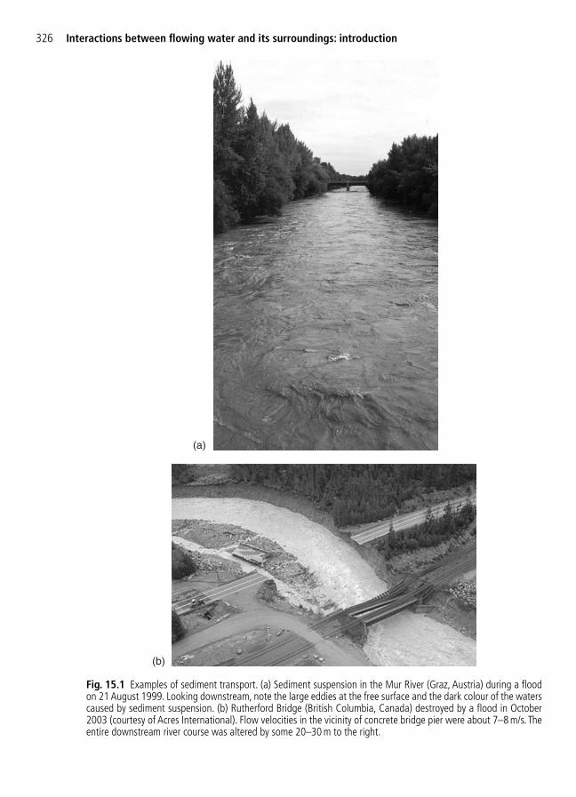
326 Interactions between flowing water and its surroundings: introduction

(a)

(b)

Fig. 15.1 Examples of sediment transport. (a) Sediment suspension in the Mur River (Graz, Austria) during a floodon 21 August 1999. Looking downstream, note the large eddies at the free surface and the dark colour of the waterscaused by sediment suspension. (b) Rutherford Bridge (British Columbia, Canada) destroyed by a flood in October2003 (courtesy of Acres International). Flow velocities in the vicinity of concrete bridge pier were about 7–8 m/s. Theentire downstream river course was altered by some 20–30 m to the right.

In Nature, air–water flows are commonly encountered at waterfalls, in mountain torrents andat wave breaking (Fig. 15.2). They are also observed in aesthetical fountains and in hydraulicstructures (e.g. Plumptre 1993, Chanson 1997) (Figs 1.2(d) and 15.2(c)). One of the first scien-tific accounts was made by Leonardo da Vinci (AD 1452–1519). In supercritical flows, air bub-bles may be entrained when the turbulent kinetic energy is large enough to overcome both surfacetension and gravity effects. The process is also called ‘white waters’. Free-surface aeration iscaused by a combination of wave instabilities and turbulence fluctuations acting next to theair–water free surface. Through this interface, there are continuous exchanges of both mass andmomentum between water and atmosphere. Figure 15.2(a) and (b) illustrates strong air entrain-ment in natural streams, while Fig. 15.2(c) shows ‘white waters’ on a stepped spillway chute.

The air–water mixing is an important re-oxygenation process, because the air bubbleentrainment increases drastically the air–water interface area, hence the air–water transferrate (Chanson 1997). In spillway design, free-surface aeration may affect the thickness offlowing water and hence sidewall design. The presence of air bubbles in shear flows mayreduce the shear stress between flow layers and induce some drag reduction. It may also prevent or reduce the damage caused by cavitation (Wood 1991, Chanson 1997).

Interactions between river waters and aquatic life are even more complex. Fish and aquaticspecies respond dynamically to river flows and changes in discharges and vegetation. Aquaticlife must account for extreme flow events ranging from long drought periods (i.e. severalyears) to very large floods (e.g. during cyclones). Flooding and riverine migration are essen-tial for the survival of many species and biodiversity of aquatic systems, but this is an inter-active process. For example, floods have significant negative impacts on fish habitats.In-stream vegetation can be removed by scouring, hence heightening competition and increas-ing susceptibility to predation. In response to these pressures, the population may declinemarkedly. But fish microhabitats may reduce the impacts of floods: e.g. fish using in-streamvegetation to mitigate the negative impacts of excessive stream flows, for predator avoidanceor reproduction. In many cases, migratory and reproductive behaviour can be triggered by

15.1 Presentation 327

(c)

Fig. 15.1 (c) Delta of the fully silted Saignon Reservoir (France) in June 1998. Looking downstream at the delta andfully silted reservoir with dam wall in far background. Dam height: 14.5 m (completed in 1961), reservoir capacity:1.4 � 105 m3, catchment area: 3.5 km2. Fully silted reservoir after 2 years of operation.

slight changes in water level, in flow velocity and sediment load (e.g. Dorava et al. 2001).While these natural processes are not yet fully understood, it is acknowledged that manyhydraulic structures act as barriers to fish migration. Figure 15.3 shows a weir and a man-madefish pass next to the left bank. In that case, however, the writer noted that, on the downstream,

328 Interactions between flowing water and its surroundings: introduction

(a)

(b)

Fig. 15.2 Examples of air entrainment in open channel flows. (a) Nishizawa-keikoku River, Yamanishi prefecture,Japan in November 1998, looking upstream. Note the ‘white waters’ in the waterfall in foreground, and in the poolin the background. (b) White waters at Le Grand Remous (Québec, Canada) on 13 July 2002. View from the PontSavoyard, looking downstream at the cascading waters and plunge point.

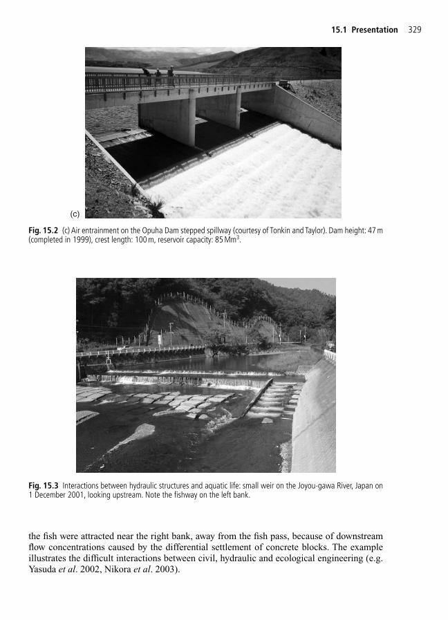
the fish were attracted near the right bank, away from the fish pass, because of downstreamflow concentrations caused by the differential settlement of concrete blocks. The exampleillustrates the difficult interactions between civil, hydraulic and ecological engineering (e.g.Yasuda et al. 2002, Nikora et al. 2003).

15.1 Presentation 329

(c)

Fig. 15.2 (c) Air entrainment on the Opuha Dam stepped spillway (courtesy of Tonkin and Taylor). Dam height: 47 m(completed in 1999), crest length: 100 m, reservoir capacity: 85 Mm3.

Fig. 15.3 Interactions between hydraulic structures and aquatic life: small weir on the Joyou-gawa River, Japan on1 December 2001, looking upstream. Note the fishway on the left bank.

15.2 Terminology

Classical (clear-water) hydraulics is sometimes referred to as fixed-boundary hydraulics. Itcan be applied to most man-made channels (e.g. concrete-lined chute) and to some extent tograssed waterways. In natural streams, the channel boundaries are movable. Movable bound-ary hydraulics applies to streams with gravel or sand beds, estuaries (i.e. silt or sand beds),sandy coastlines and man-made canals in earth, sand or gravel. Movable boundary hydraulicsis characterized by variable boundary roughness and variable channel dimensions. Stronginteractive processes between the water flow and the bed form changes take place. Accretion,or deposition, refers to an increase of channel bed elevation resulting from the accumulationof sediment deposits. Scour or erosion is the removal of bed material caused by the erodingpower of the flow. Sediment transport is the general term used for the transport of material(e.g. silt, sand, gravel, boulder) in rivers and streams. The transported material is called thesediment load. Distinction is made between the bed load and the suspended load. The bedload characterizes grains rolling along the bed while suspended load refers to grains main-tained in suspension by turbulence. The distinction is however sometimes arbitrary whenboth loads are of the same material.

White water is the non-technical term used to design free-surface aerated flows. Therefraction of light by the entrained air bubbles gives the ‘whitish’ appearance to the free sur-face of the flow. Natural aeration occurring at the free surface of high-velocity flows isreferred to as free-surface aeration or self-aeration.

15.3 Structure of this section

In Part 4, sediment processes are discussed in Chapter 16. Free-surface aeration and ‘whitewaters’ are dealt with in Chapter 17. Both chapters present introductory material that must becomplemented by expert references.

330 Interactions between flowing water and its surroundings: introduction

16

Interaction between flowingwater and solid boundaries:sediment processes

SummaryThis chapter deals with sediment motion in open channel flows primarily. Aftersome basic definitions, both bed-load and suspension processes are discussed.Later complete calculations are developed.

16.1 Introduction

Numerous failures resulted from the inability of engineers to predict sediment motion: e.g.bridge collapse (pier foundation erosion), formation of sand bars in estuaries and navigablerivers, destruction of banks and levees (Fig. 15.1). In most cases, river and stream flowsbehave as quasi-steady gradually varied flows and the flow conditions are very close to uni-form equilibrium flow conditions. Application of the momentum equation provides anexpression of the mean flow velocity V at equilibrium:

(16.1)

where f is the Darcy friction factor, � is the bed slope and DH is the hydraulic diameter.The knowledge of the velocity profile, more specifically of the velocity next to the chan-

nel bed, is further required to predict accurately the occurrence of sediment motion. For analluvial stream, the bed roughness effect might be substantial (e.g. in a gravel-bed stream)and the velocity profile is affected by the ratio of the sediment size to the inner wall regionthickness: i.e. ds/(10(�/V*)) where ds is the sediment size, � is the water kinematic viscosityand V* is the shear velocity. If the sediment size is small compared to the sub-layer thickness(i.e. V*(ds/ ) � 4–5), the flow is smooth turbulent. If the sediment size is much larger than the

Vgf

D

8

4 sin Uniform equilibrium flowH� �

sub-layer thickness (i.e.V*(ds/�) � 75–100), the flow is called fully rough turbulent. In firstapproximation, the velocity distribution may be approximated by a power law function:

(16.2)

where Vmax is the free-surface velocity, d is the water depth, y is the distance normal to thebed and N is a function of the boundary roughness: where f is the Darcy friction factor and K is a constant (K � 0.4).

Forces acting on a sediment particleIn open channel flows, the forces acting on each sediment particle are the gravity and buoyancyforces, the drag and lift forces, and the reaction forces of the surrounding grains (Fig. 16.1).The gravity force and the buoyancy force act both in the vertical direction. The drag forceacts in the flow direction while the lift force in the direction perpendicular to the flow direction.The inter-granular forces are related to the grain disposition and packing.

N f K 8�

V

max

1

V

yd

N

�

332 Interaction between flowing water and solid boundaries: sediment processes

Lift force

Drag forceBuoyancy force

Gravity force

V

Fig. 16.1 Forces acting on a sediment particle; the inter-granular forces are not shown for clarity.

Notes1. The hydraulic diamater is defined as: DH � 4(A/Pw) where A is the flow cross-sectional

area and Pw is the wetted perimeter. DH is also called the equivalent pipe diameter.2. The constant K is called the von Karman constant after Theodore von Karman. It is a

constant of proportionality between the Prandtl mixing length and the distance fromthe boundary. Experimental results give: K � 0.40.

3. Theodore von Karman (or von Kármán) (1881–1963) was a Hungarian fluid dynami-cist and aerodynamicist who worked in Germany (1906–1929) and later in USA. Hewas a student of Ludwig Prandtl in Germany. He gave his name to the vortex shed-ding behind a cylinder (Karman vortex street).

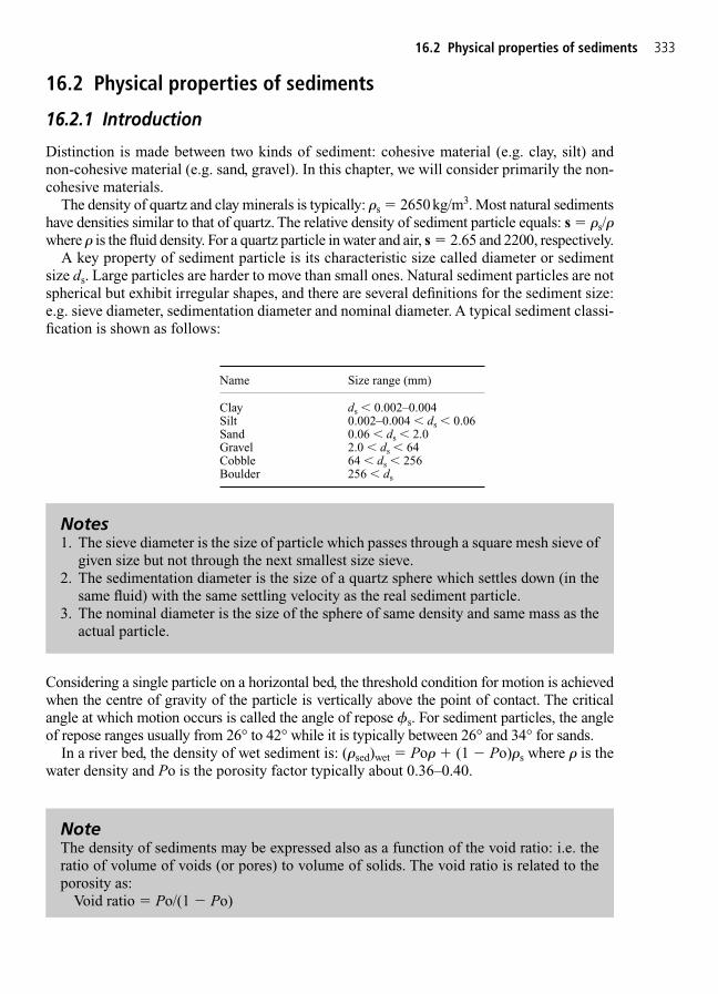
16.2 Physical properties of sediments

16.2.1 Introduction

Distinction is made between two kinds of sediment: cohesive material (e.g. clay, silt) andnon-cohesive material (e.g. sand, gravel). In this chapter, we will consider primarily the non-cohesive materials.

The density of quartz and clay minerals is typically: �s � 2650 kg/m3. Most natural sedimentshave densities similar to that of quartz. The relative density of sediment particle equals: s � �s/�where � is the fluid density. For a quartz particle in water and air, s � 2.65 and 2200, respectively.

A key property of sediment particle is its characteristic size called diameter or sedimentsize ds. Large particles are harder to move than small ones. Natural sediment particles are notspherical but exhibit irregular shapes, and there are several definitions for the sediment size:e.g. sieve diameter, sedimentation diameter and nominal diameter. A typical sediment classi-fication is shown as follows:

Considering a single particle on a horizontal bed, the threshold condition for motion is achievedwhen the centre of gravity of the particle is vertically above the point of contact. The criticalangle at which motion occurs is called the angle of repose s. For sediment particles, the angleof repose ranges usually from 26° to 42° while it is typically between 26° and 34° for sands.

In a river bed, the density of wet sediment is: (�sed)wet � Po� (1 � Po)�s where � is thewater density and Po is the porosity factor typically about 0.36–0.40.

16.2 Physical properties of sediments 333

Name Size range (mm)

Clay ds � 0.002–0.004Silt 0.002–0.004 � ds � 0.06Sand 0.06 � ds � 2.0Gravel 2.0 � ds � 64Cobble 64 � ds � 256Boulder 256 � ds

Notes1. The sieve diameter is the size of particle which passes through a square mesh sieve of

given size but not through the next smallest size sieve.2. The sedimentation diameter is the size of a quartz sphere which settles down (in the

same fluid) with the same settling velocity as the real sediment particle.3. The nominal diameter is the size of the sphere of same density and same mass as the

actual particle.

NoteThe density of sediments may be expressed also as a function of the void ratio: i.e. theratio of volume of voids (or pores) to volume of solids. The void ratio is related to theporosity as:

Void ratio � Po/(1 � Po)

16.2.2 Particle fall velocity

In a fluid at rest, a suspended particle heavier than water has a downward motion. The term-inal fall velocity of the particle is its velocity when the sum of the gravity force, buoyancyforce and fluid drag force equals zero. For a spherical particle settling in a still fluid, the term-inal fall velocity wo equals:

(16.3)

where ds is the particle diameter, Cd is the drag coefficient and s � �s/�. The negative signindicates a downward motion for s � 1. A re-analysis of numerous experimental data withspherical particles that were unaffected by sidewall effects yielded:

Spherical particles (Re � 2 � 105)

where Re is the particle Reynolds numbers: Re � wo(ds/�) and � is the fluid kinematic viscos-ity (Brown and Lawler 2003).

For natural sand and gravel particles, experimental values of drag coefficient were best fit-ted by (Cheng 1997):

Natural sediment particles (Re � 1 � 104) (16.4)

The terminal fall velocity of a sediment particle may be estimated by combining equations(16.3) and (16.4). Computed values for natural sediment particles were compared favourablywith experimental data (e.g. Engelund and Hansen 1972), and typical values are reportedbelow.

CRed 24

1�

2 33 2

CRe

Re

Re

d 24

(1 0.150 0.407

1 8710

�

0 681. )

wgdCo

s

d

4

( 1)� � �3

s

334 Interaction between flowing water and solid boundaries: sediment processes

ds (m) Re Cd wo (m/s)

0.0001 7.6 � 10�1 36.2 0.0080.0002 4.6 � 100 8.0 0.0230.0005 3.3 � 101 2.4 0.0670.001 1.2 � 102 1.6 0.1170.002 3.7 � 102 1.3 0.1860.005 1.6 � 103 1.1 0.3140.01 4.5 � 103 1.0 0.4540.02 1.3 � 104 1.0 0.6500.05 5.1 � 104 1.0 1.0340.1 1.5 � 105 1.0 1.4660.2 4.1 � 105 1.0 2.075

Notes: s � 2.65; wo: terminal fall velocity of single particle in waterat 20°C.

DiscussionLarge-size particles fall faster than small particles. At the limits, the relationship between fallvelocity and particle size must satisfy:

Laminar flow motion (wo(ds/�) �� 1)

Turbulent flow motion (wo(ds/�) � 1000)

However the settling velocity of a single particle may be affected by the presence of sur-rounding particles. Experiments showed that thick homogeneous suspensions have a slowerfall velocity than that of a single particle. This effect, called hindered settling, results from theinteraction between the downward fluid motion induced by each particle on the surroundingfluid and the return flow (i.e. upward fluid motion) following the passage of a particle. As aparticle settles down, a volume of fluid equal to the particle volume is displaced upwards.

16.3. Threshold of sediment bed motion

16.3.1 Introduction

The term threshold of sediment motion describes the flow and boundary conditions for whichthe transport of sediment starts to occur. The threshold of sediment motion cannot be definedwith an exact (absolute) precision but most experimental observations provide reasonablyconsistent results.

The inception of sediment motion is related to the boundary shear stress �o. Considering agiven channel and bed material, no sediment motion is observed at very low bed shear stressuntil the shear stress �o exceeds a critical value (�o)c. For �o larger than the critical value, bed-load motion takes place (e.g. Fig. 16.2). The grain motion along the bed is not smooth, andsome particles bounce and jump over the others. With increasing shear velocities, the numberof particles bouncing and rebounding increases until the cloud of particles becomes asuspension.

w do s�

w do s2�

16.3 Threshold of sediment bed motion 335

NotesThe average shear stress on the wetted surface or boundary shear stress equals:

where f is the Darcy friction factor and V is the mean flow velocity. The shear velocityV* is defined as:

where �o is the boundary shear stress and � is the density of the flowing fluid. The shearvelocity is a measure of shear stress and velocity gradient near the boundary.

V* o��

�

� �o2

8�

fV

16.3.2 Threshold of bed-load motion

Particle movement occurs when the moments of the destabilizing forces (i.e. drag, lift, buoy-ancy) with respect to the point of contact become larger than the stabilizing moment of theweight force. Experimental observations highlighted the importance of the Shields parameter�* which may be derived from dimensional analysis:

(16.5)

A critical value of the Shields stability parameter may be defined at the inception of bed-loadmotion: i.e. �* � (�*)c. Bed-load motion occurs for: �* � (�*)c. Basically bed-load transportoccurs when the boundary shear stress �o is larger a critical value: (�o)c � �(s � 1)gds(�*)c.Experimental observations showed that the critical Shields parameter (�*)c is primarily afunction of the shear Reynolds number (ds(V*/�)) (Fig. 16.3).

��

�*

( 1) o

s

��s gd

336 Interaction between flowing water and solid boundaries: sediment processes

Fig. 16.2 Bed-load material in the Hayagawa Catchment (Japan) in November 1998; the Haya River is a tributaryof the Fuji River.

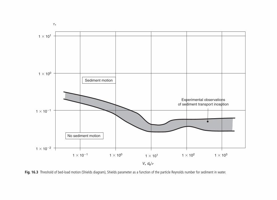
1 � 101

1 � 100

1 � 10�2

1 � 10�1

1 � 10�1 1 � 100 1 � 101 1 � 102 1 � 103

Sediment motion

Experimental observationsof sediment transport inception

t*

V* ds/n

No sediment motion

Fig. 16.3 Threshold of bed-load motion (Shields diagram), Shields parameter as a function of the particle Reynolds number for sediment in water.

16.3.3 Initiation of sediment suspension

Considering a particle in suspension, the particle motion in the direction normal to the bed isrelated to the balance between the particle fall velocity component (wocos �) and the turbu-lent velocity fluctuation in the direction normal to the bed. The latter is of the same order ofmagnitude as the shear velocity V*. In Fig. 16.4, some suspended sediment load is high-lighted by the brownish colour of the flow.

Based upon the experimental observations, a simple criterion for the initiation of suspen-sion is:

Sediment suspension (16.6)

The flow conditions at onset of sediment suspension are summarized in Fig. 16.5. This modi-fied Shields diagram presents the Shields parameter �* as a function of a dimensionless par-ticle parameter d* � ds

3��(s � 1)���g/�2� (Fig. 16.5). The critical Shields parameter for initiationof bed-load motion is also plotted in solid line.

Vw

*

o

0.2–2�

338 Interaction between flowing water and solid boundaries: sediment processes

Notes1. The stability parameter �* is called commonly the Shields parameter after A. Shields

who introduced it first. (�*)c is commonly called the critical Shields parameter.2. The stability parameter may be rewritten as:

DiscussionFor given fluid and sediment properties, and given boundary shear stress, the Shieldsparameter �* decreases with increasing sediment size: i.e. �* � 1/ds. For given flow conditions, sediment motion may occur for small particle sizes while no particle motionoccurs for large grain sizes. The particle size distribution has an effect when the size range is wide. After an initial erosion of the fine particles, the coarser particles will form an armour layer preventing further erosion. This process is called bed armouring. Basically the fine particles become shielded by the larger particles (i.e. bedarmour).

On steep channels, the bed slope assists in destabilizing the particles and bed motionoccurs at lower bed shear stresses than in flat channels. At the limit, when the bed slopebecomes larger than the repose angle, the grains roll even in absence of flow, i.e. the bedslope is unstable.

For clay and silty sediment beds, the cohesive forces between sediment particles maybecome important. This causes a substantial increase of the bed resistance to scouring.

��

�*

* ( 1)

( 1)s

o

s

��

��

Vgd gd

2

s s

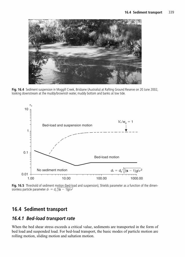
16.4 Sediment transport

16.4.1 Bed-load transport rate

When the bed shear stress exceeds a critical value, sediments are transported in the form ofbed load and suspended load. For bed-load transport, the basic modes of particle motion arerolling motion, sliding motion and saltation motion.

16.4 Sediment transport 339

Fig. 16.4 Sediment suspension in Moggill Creek, Brisbane (Australia) at Rafting Ground Reserve on 20 June 2002,looking downstream at the muddy/brownish water, muddy bottom and banks at low tide.

0.01

0.1

1

10

1.00 10.00 100.00 1000.00

t*

d* � ds No sediment motion

Bed-load motion

Bed-load and suspension motionV*/wo � 1

(s � 1)g/n23

Fig. 16.5 Threshold of sediment motion (bed-load and suspension), Shields parameter as a function of the dimen-sionless particle parameter d* � ds

3��(s �� 1)�g/��2�

Bed-load transport is closely associated with inter-granular forces. It takes place in a thinregion of fluid close to the bed called bed-load layer. The bed-load transport rate per unitwidth may be defined as:

Bed-load transport (16.7)

where Cs is the mean sediment concentration in the bed-load layer, s is its thickness, and Vsis the average sediment velocity in the bed-load layer. A simple model yields (Nielsen 1992):

Cs � 0.65

DiscussionSeveral researchers proposed formulae to estimate the characteristics of the bed-load layer.Overall the results are not consistent and there is great uncertainty.

The prediction of bed-load transport rate is not an accurate prediction. One researcherstated explicitly that: “the overall inaccuracy […] may not be less than a factor 2” (van Rijn1984).

16.4.2 Suspension transport rate

Sediment suspension can be described as the motion of sediment particles during which theparticles are surrounded by fluid. The grains are maintained within the mass of fluid by tur-bulent agitation without (frequent) bed contact. The amount of particles transported by sus-pension is called the suspended load.

In a stream with particles heavier than water, the sediment concentration is larger next tothe bottom and turbulent mixing induces an upward migration of the grains to region of lowerconcentrations. A time-averaged balance between settling and diffusive flux derives from thecontinuity equation for sediment matter:

(16.8)

where Cs is the local sediment concentration at a distance y measured normal to the channelbed, DS is the sediment diffusivity and wo is the particle settling velocity. In natural (flowing)streams, the turbulence is generated by boundary friction: it is stronger close to the channelbed than near the free surface.

Assuming the sediment diffusivity to be nearly equal to the momentum exchange coeffi-cient (i.e. ‘eddy viscosity’), the sediment diffusivity Ds may be estimated as:

D V d yyds K ( ) � * �

Dy

wC

Css

o sdd

cos � � �

VV

s 4.8*

�

� �s

sc 2.5 ( (

d� �* * ) )

q C Vs s s s �

340 Interaction between flowing water and solid boundaries: sediment processes

where d is the flow depth, V* is the shear velocity and K is the von Karman constant(K � 0.4). The integration of equation (16.8) gives the distribution of sediment concentra-tion across the flow depth:

s � y � d (16.9)

where Cs is the reference sediment concentration in the bed-load layer (y � S) (paragraph16.4.1).

The suspended-load transport rate equals:

Sediment load (16.10)

where qs is the volumetric suspended-load transport rate per unit width, Cs is the sedimentconcentration (equation (16.9)), V is the local velocity at a distance y measured normal to thechannel bed (equation (16.2)), d is the flow depth and s is the bed-load layer thickness.

RemarksWhen both bed-load motion and suspension take place, the total sediment transport rate maybe calculated using equations (16.7) and (16.10). The result is called the sediment transportcapacity. It is not always equal to the observed sediment motion (see next section).

16.5 Total sediment transport rate

16.5.1 Presentation

The total sediment discharge is the total volume of sediment particles in motion per unittime. It includes the sediment transport by bed-load motion and by suspension. In Section16.4, the sediment transport capacity of a known bed sediment mixture was estimated:

Sediment transport capacity (16.11)q C V yCd

s s s s s dVs

� ∫

q yCd

s s dVs

� ∫

C C

dyd

w V

s s

s

cos /(K

1

1

o

�

�

�

� * )

16.5 Total sediment transport rate 341

DISCUSSIONEquation (16.9) was first developed by Rouse (1937) and it was successfully verifiedwith laboratory and field data. Suspension takes place above the bed-load layer. Hencea logical choice for the limiting conditions of the integration of equation (16.8) is theouter edge of the bed-load layer.

Although equation (16.9) was successfully compared with numerous data, its deriv-ations implies a parabolic distribution of the sediment diffusivity. The re-analysis ofmodel and field data (e.g. Anderson 1942, Coleman 1970) shows that the sediment dif-fusivity distribution is better estimated by a semi-parabolic profile:

y/d � 0.5

y/d � 0.5D V ds 0.1� *

D V d yyds K ( ) � * �

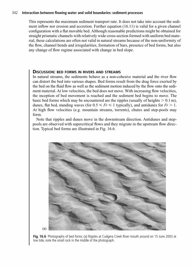
This represents the maximum sediment transport rate. It does not take into account the sedi-ment inflow nor erosion and accretion. Further equation (16.11) is valid for a given channelconfiguration with a flat movable bed. Although reasonable predictions might be obtained forstraight prismatic channels with relatively wide cross-section formed with uniform bed mate-rial, these calculations are often not valid in natural streams because of the non-uniformity ofthe flow, channel bends and irregularities, formation of bars, presence of bed forms, but alsoany change of flow regime associated with change in bed slope.

342 Interaction between flowing water and solid boundaries: sediment processes

DISCUSSION: BED FORMS IN RIVERS AND STREAMSIn natural streams, the sediments behave as a non-cohesive material and the river flow can distort the bed into various shapes. Bed forms result from the drag force exerted bythe bed on the fluid flow as well as the sediment motion induced by the flow onto the sedi-ment material. At low velocities, the bed does not move. With increasing flow velocities,the inception of bed movement is reached and the sediment bed begins to move. Thebasic bed forms which may be encountered are the ripples (usually of heights � 0.1 m),dunes, flat bed, standing waves (for 0.5 " Fr " 1 typically), and antidunes for Fr � 1.At high flow velocities (e.g. mountain streams, torrents), chutes and step-pools mayform.

Note that ripples and dunes move in the downstream direction. Antidunes and step-pools are observed with supercritical flows and they migrate in the upstream flow direc-tion. Typical bed forms are illustrated in Fig. 16.6.

(a)

Fig. 16.6 Photographs of bed forms. (a) Ripples at Cudgera Creek River mouth around on 15 June 2003 atlow tide, note the small rock in the middle of the photograph.

16.5 Total sediment transport rate 343

(c)

Fig. 16.6 (b) Dune bed forms in a small stream, flow from right to left. (c) Standing wave flow with standingwave bed forms at Serizawa Beach (Japan) in March 1999, looking upstream.

(b)

16.5.2 Flow resistance in natural systems

In alluvial streams the mean boundary shear stress �o may be expressed as:

(16.12)

where ��o is the skin friction shear stress and ��o is the form-related shear stress. The skin fric-tion shear stress equals:

where � is the fluid density, V is the mean flow velocity and f is the Darcy–Weisbach frictionfactor. The bed-form shear stress ��o is related to the fluid pressure distribution on the bedform and to the form loss. The form loss may be crudely analysed as a sudden expansiondownstream of the bed-form crest. For a two-dimensional bed-form element, it yields:

where h and l are respectively the bed-form height and length (e.g. Chanson 1999a, 2004b).

′′� �o2

2

12

� Vhld

′� �o2

8�

fV

� � �o o o � ′ ′′

344 Interaction between flowing water and solid boundaries: sediment processes

(d)

Fig. 16.6 (Contd ) (d) Supercritical flow with large antidune bed forms at Serizawa Beach (Japan) in a rip chan-nel leading into breaking waves; Terasawa Beach (Japan) on 13 October 2001, looking downstream.

Importantly the bed-load transport must be related to the effective shear stress (skin frictionshear stress) only and not to the form roughness. In natural rivers, the Shields parameter andbed-load layer characteristics must be calculated using the skin friction bed shear stress. Theonset of sediment motion and bed-load transport rate are predicted using the Shields parameterdefined as:

For the suspended material, the sediment concentration and velocity distribution propertiesare related of the total bed shear stress �o. That is, the Rouse number (wocos �/(KV*)), theshear velocity V* and the mean flow velocity V are calculated in terms of the mean boundaryshear stress .

16.5.3 Design calculations

The interactions between sediment transport, bed-form and flow properties are extremely com-plicated. For complete calculations, Engelund and Hansen (1967) developed a simple designchart which regroups the relevant parameters: i.e. the Froude number (Vd)/��g(s ��� 1)��ds

3, thedimensionless sediment transport rate qs/��g(s ��� 1)��ds

3, the bed slope So � sin �, the dimen-sionless flow depth d/ds, and the bed form (Fig. 16.7). This design chart was developed forfully rough turbulent flows and it was validated with experimental data.

ApplicationThe most important variables in designing alluvial channels are the water discharge Q, thesediment transport rate Qs and the sediment size ds. Calculations of flow properties and sedi-ment transport are deduced by an iterative process. In a first stage, simplified design charts(e.g. Engelund and Hansen 1967, Fig. 16.7) may be used to ‘guess’ the type of bed form. Ina second stage, complete calculations must be developed to predict the hydraulic flow condi-tions (V, d), the type of bed forms and the sediment transport capacity. Then the continuityequation for sediment material may be used to assess the rate of erosion (or accretion).

For a prismatic section of alluvial channel, complete calculations include several succes-sive steps:

1. Determination of the channel characteristics (bed slope, cross-sectional shape, movablebed properties).

2. Selection of inflow conditions (discharge Q, sediment inflow).3. Calculations of sediment-laden flow properties.

� � �o o o � ′ ′′

��

�*

o

s

( 1)

��

′g ds

16.5 Total sediment transport rate 345

Notes1. Figure 16.7 takes into account the effect of bed forms and it may be used also to pre-

dict the type of bed form.2. In the design chart, the sediment size is the median grain size ds � d50 (Fig. 16.7).3. Calculations are not valid for ripple bed forms with dsV*/� � 12.

1�103

1�104

1�105

1�106

1�10�2 1�10�1 1 1�101 1�102 1�103

Vd

g (s � 1)ds3

qs

g (s � 1)ds3d/ds�4�102

sin u� 1�10�5

d/ds�1�105

8�104

6�104

3�104

2�104

1.5�104

1�104

8�103

d/ds�6�103

4�104

4�103

3�103

2�103

1.5�103

8�102

6�102

3�102

1�103

1.5�10�5

2�10�5 3�10�54�10�5

6�10�58�10�5

1�10�4

1.5�10�4

2�10�4

3�10�4

4�10�4 � sin u

6�10�4

8�10�4

1�10�3

1.5�10�3 � sin u

2�10�3

3�10�3

4�10�3 � sin u

Step-pool

Anti-d

unes

Transitionand

Flat bed

Fig. 16.7 Open channel flow with movable boundaries, pre-design calculations (Engelund and Hansen 1967).

3.1. Preliminary calculations assuming a flat bed, uniform equilibrium flow and kS � dS

yield some estimate of flow properties (V and d ) and bed shear stress �o, and of theoccurrence of sediment motion.

3.2. Pre-design calculations to assess type of bed form using the design chart ofEngelund and Hansen (1967) (Fig. 16.7).

3.3. Flow calculation iterations until the type of bed form, bed resistance and flow con-ditions satisfy the continuity and momentum equations.

3.4. Sediment transport calculations include an estimate of the sediment transport cap-acity (equation (16.11)) and the application of the continuity equation for the sedimentmaterial to predict erosion or accretion.

16.6 Exercises

1. The dry density of a sand mixture is 1725 kg/m3. Calculate the sand mixture porosityand the wet density of the mixture (and give units).

2. Considering a natural stream, the water discharge is 6.4 m2/s and the observed flowdepth is 4.2 m. What is most likely type of bed form with a movable bed?

3. Considering a 1.2 mm sediment particle settling in water at 20°C, calculate the set-tling velocity.

4. Considering a stream with a flow depth of 3.2 m and a bed slope sin � � 0.0002, themedian grain size of the channel bed is 2.5 mm. Calculate the flow properties and pre-dict the occurrence of sediment motion. (Assume that the equivalent roughnessheight of the channel bed equals the median grain size and that uniform equlibriumfow conditions are achieved.)

5. Considering a stream with a flow depth of 1.8 m and a bed slope sin � � 0.0015, themedian grain size of the channel bed is 0.85 mm. Predict the occurrence of bed-loadmotion and of suspension. (Assume that the equivalent roughness height of the chan-nel bed equals the median grain size.)

6. A stream carries a discharge of 58 m3/s. The channel is 33 m wide and the longitudinalbed slope is 9 m/km. The bed consists of a mixture of fine sands (d50 � 1.1 mm).Assume that uniform equilibrium flow conditions are achieved. Calculate the flowproperties, the occurrence of sediment motion and the sediment transport rate capacity.

7. A 20 m wide channel has a bed slope of 0.0011. The bed consists of a mixture of lightparticle (�s � 2350 kg/m3) with a median particle size d50 � 1.32 mm. The flow rateis 6.4 m3/s. Calculate the bed-load transport rate at uniform equilibrium flow condi-tions. (Assume that the equivalent roughness height of the channel bed equals themedian grain size.) Predict the suspended sediment transport rate.

8. Considering a 2000 m reach of an alluvial channel (55 m wide), the median grain sizeof the movable bed is 0.8 mm and the longitudinal bed slope is sin � � 0.000 33. Theobserved flow depth is 1.41 m and the mean sediment concentration of the inflow is1.8%. Calculate the total sediment transport capacity and the rate of erosion (oraccretion). (Assume uniform equilibrium flow conditions. Take into account the bedform and use the design chart of Engelund and Hansen (1967) to predict the type ofbed form. Assume ks � 3d50.)

16.6 Exercises 347

17

Interaction between flowingwater and free surfaces:self-aeration and air entrainment

SummaryIn this chapter, the mechanisms of free-surface aeration in turbulent flows arereviewed. Then dimensional analysis and similitude are developed including a discussion of scale effects affecting physical modelling. Measurementstechniques are presented. Later simple applications are developed.

17.1 Introduction

Air–water flows have been studied recently compared to classical fluid mechanics. Althoughsome researchers observed free-surface aeration and discussed possible effects (e.g.Leonardo da Vinci), the first successful experimental investigations were conducted duringthe mid-20th century: i.e. Ehrenberger (1926) in Austria and Straub and Anderson (1958) inNorth America. The latter data set is still widely used by engineers and researchers. Anothermilestone was the series of prototype experiments performed on the Aviemore Dam spillway inNew Zealand under the supervision of I.R. Wood (Cain and Wood 1981). Laboratory and proto-type investigations showed the complexity of the free-surface aeration process. Ian R. Wood fur-ther developed the basic principles of modern self-aerated flow calculations (e.g. Wood 1991).Recent developments were discussed in Falvey (1980), Wood (1991) and Chanson (1997a).

17.2 Free-surface aeration in turbulent flows:basic mechanisms

17.2.1 Presentation

Air entrainment, or free-surface aeration, is defined as the entrainment/entrapment of un-dissolved air bubbles and air pockets that are carried away within the flowing fluid (Fig. 17.1).

(a)

(b)

(c)

Fig. 17.1 Photographs of free-surface aeration in open channel flows. (a) Cascading waters at Craddle Mountain,Tasmania in July 2002 (courtesy of York-wee Tan and Jerry Lim). (b) Mount Crosby Weir overflow on 5 September1999 – note free-surface aeration down the steep chute and at the plunge point at chute toe. (c) Jiroft Dam spillwayoperation (Iran) (courtesy of Amir Aghakoochak). Note the dark colour of water suggesting heavy sediment suspension.

350 Interaction between flowing water and free surfaces

The resulting air–water mixture consists of both air packets within water and water dropletssurrounded by air. It also includes spray, foam and complex air–water structures. In turbulentflows, there are two basic types of air entrainment process. The entrainment of air packets canbe localized or continuous along the air–water interface (Fig. 17.2). Examples of local aera-tion include air entrainment by plunging jet and at hydraulic jump. Air bubbles are entrainedlocally at the intersection of the impinging jet with the surrounding waters (Fig. 17.2(a)). Theintersecting perimeter is a singularity in terms of both air entrainment and momentumexchange, and air is entrapped at the discontinuity between the high-velocity jet flow and thereceiving pool of water. Interfacial aeration (or continuous aeration) is defined as the airentrainment process along an air–water interface, usually parallel to the flow direction: e.g.in chute flows (Figs 17.1 and 17.2(b)). An intermediate case is a high-velocity water jets discharging into air. The nozzle is a singularity, characterized by a high rate of aeration, followed by some interfacial aeration downstream at the jet free surfaces (Figs 17.1(c) and 17.2(c)).

17.2.2 Local/singular aeration mechanism: air entrapment at plunging jets

With local (singular) aeration, air entrainment results from some discontinuity at the impinge-ment perimeter: e.g. plunging water jets, hydraulic jump flows (Fig. 17.3). One basic exampleis the vertical plunging jet (Figs 17.2(a) and 17.3). At plunge point, air may be entrapped whenthe impacting flow conditions exceed a critical threshold (McKeogh 1978, Ervine et al. 1980,Cummings and Chanson 1999). McKeogh (1978) showed first that the flow conditions atinception of air entrainment are functions of the jet turbulence level. For a given plunging jetconfiguration, the onset velocity increases with decreasing jet turbulence. For vertical waterjets, the dimensionless onset velocity may be correlated by:

(17.1)

where Ve is the onset velocity, �w is the liquid dynamic viscosity, is the surface tension andTu is the ratio of the standard deviation of the jet velocity fluctuations about the mean to thejet impact velocity.

For jet impact velocities slightly larger than the onset velocity, air is entrained in the formof individual bubbles and packets. The entrained air may have the form of ‘kidney-shaped’bubbles which may break-up into two ‘daughter’ bubbles, ‘S-shape’ packets, or elongated ‘fin-gers’ that may break-up to form several small bubbles by a tip-streaming mechanism, dependingupon the initial size of the entrained air packet. The air entrainment rate is very small, hardlymeasurable with phase detection intrusive probes. At higher impact velocities, the amount ofentrained air becomes significant and the air diffusion layer is clearly marked by the whiteplume generated by the entrained bubbles (Fig. 17.3(b) and (c)). Air entrainment is an unsteadyrapidly varied process. An air cavity is set into motion between the impinging jet and the sur-rounding fluid and it is stretched by turbulent shear (Fig. 17.3(a)). The air cavity behaves asa ventilated air sheet and air pockets are entrained by discontinuous gusts at the lower tip ofthe elongated air cavity.

VTue w 0.0109(1 3.375 exp( 80 ))

�

� �

Entrainedair bubbles

C, V

x

y

Inductiontrumpet

V

x1

Momentumshear layer

Air diffusion layer

Developing

flow region

(advective diffusionregion)

Very-near

flow region

C � 0

Air–waterflow region

V1d1

Water jet

Surrounding atmosphere

Localaeration

Interfacial aeration

Nozzle

xy

Air–water projection

Foam

Intermediateregion

Bubblyflow

region

Air bubblecluster

C, F0.9

Y90

y

uF

C

Air packet

Sprayregion

Fig. 17.2 Sketch of basic free-surface aeration processes.

17.2 Free-surface aeration in turbulent flows: basic mechanisms 351

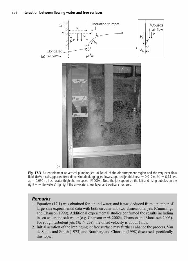
352 Interaction between flowing water and free surfaces

V

V1

d1y

x1Induction trumpet

dal

Vi

H

Elongatedair cavity

V1

dal

Vi

Couetteair flow

(a)

(b)

Fig. 17.3 Air entrainment at vertical plunging jet. (a) Detail of the air entrapment region and the very-near flowfield. (b) Vertical supported (two-dimensional) plunging jet flow: supported jet thickness � 0.012 m, V1 � 6.14 m/s,x1 � 0.090 m, fresh water (high-shutter speed 1/1000 s). Note the jet support on the left and rising bubbles on theright – ‘white waters’ highlight the air–water shear layer and vortical structures.

Remarks1. Equation (17.1) was obtained for air and water, and it was deduced from a number of

large-size experimental data with both circular and two-dimensional jets (Cummingsand Chanson 1999). Additional experimental studies confirmed the results includingin sea water and salt water (e.g. Chanson et al. 2002a, Chanson and Manasseh 2003).For rough turbulent jets (Tu � 2%), the onset velocity is about 1 m/s.

2. Initial aeration of the impinging jet free surface may further enhance the process. Vande Sande and Smith (1973) and Brattberg and Chanson (1998) discussed specificallythis topic.

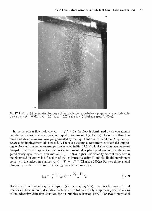
In the very-near flow field (i.e. (x � x1)/d1 � 5), the flow is dominated by air entrapmentand the interactions between gas and liquid entrainment (Fig. 17.3(a)). Dominant flow fea-tures include an induction trumpet generated by the liquid entrainment and the elongated aircavity at jet impingement (thickness al). There is a distinct discontinuity between the imping-ing jet flow and the induction trumpet as sketched in Fig. 17.3(a) which shows an instantaneous‘snapshot’ of the entrapment region. Air entrainment takes place predominantly in the elon-gated cavity by a Couette flow motion (Fig. 17.3(a), right). The velocity discontinuity acrossthe elongated air cavity is a function of the jet impact velocity V1 and the liquid entrainmentvelocity in the induction trumpet Vi: Vi � (V1 � Ve)

0.15 (Chanson 2002a). For two-dimensionalplunging jets, the air entrainment rate qair may be estimated as:

(17.2)

Downstream of the entrapment region (i.e. (x � x1)/d1 � 5), the distributions of voidfractions exhibit smooth, derivative profiles which follow closely simple analytical solutionsof the advective diffusion equation for air bubbles (Chanson 1997). For two-dimensional

q V yV V

d

dair air

1 ial d

al��

1

1

2∫ �

(c)

Fig. 17.3 (Contd ) (c) Underwater photograph of the bubbly flow region below impingement of a vertical circularplunging jet – d1 � 0.012 m, V1 � 2.5 m/s, x1 � 0.05 m, sea water (high-shutter speed 1/1000 s).

17.2 Free-surface aeration in turbulent flows: basic mechanisms 353

354 Interaction between flowing water and free surfaces

vertical jets, it yields:

(17.3)

where x is the streamwise direction, y is the distance normal to the jet centreline, x1 is thefree-jet length, V1 is the jet velocity at impingement, qair is the air flow rate per unit width, qwis the water discharge per unit width, D# is a dimensionless air bubble diffusivity and d1 is thejet thickness at impact. (Full details of the integration are given in Appendix A, Section 17.6.)

With circular plunging jets, the analytical solution of the advective diffusion equationbecomes:

(17.4)

where Io is the modified Bessel function of the first kind of order zero (Appendix A,Section 17.6).

17.2.3 Interfacial aeration process: self-aeration down a steep chute

Examples of interfacial aeration include spillway chute flows and ‘white waters’ down a moun-tain stream (Figs 17.1(a), (b), 17.2(b) and 17.4). On smooth and stepped (skimming flow) chutes,

CQQ

Dx x

rD

rr

x xr

ID

rr

x xr

1

4

exp1

4

1

air

w # 1#

1o #

1�

��

� �

1

1

2

1

1

1

1

2

Cqq

Dx x

d

D

yd

x xd

D

yd

x xd

12

1

4

exp1

4

1

exp

1

4

1

air

w # 1

#1

1#

1

1

��

� �

�

� �

�

�1

2

1

2

1

Remarks1. The void fraction or air concentration is defined as the volume of air per unit volume

of air and water. In clear water, C � 0 and C � 1 in air.2. Cummings and Chanson (1997a) and Brattberg and Chanson (1998) presented suc-

cessful comparisons between equation (17.3) and experimental data. Chanson andManasseh (2003) and Chanson et al. (2002a) compared successfully equation (17.4)with experimental data.

3. Estimates of dimensionless diffusivity D# and air flow rate Qair/Qw are discussed inAppendix A (Section 17.6).

DiscussionPlunging jet entrainment is a highly efficient mechanism for producing large gas–liquidinterfacial areas. Applications include minerals-processing flotation cells, waste-watertreatment, oxygenation of mammalian-cell bio-reactors and riverine re-oxygenation weirs.Another form of plunging jet is the plunging breaking waves.

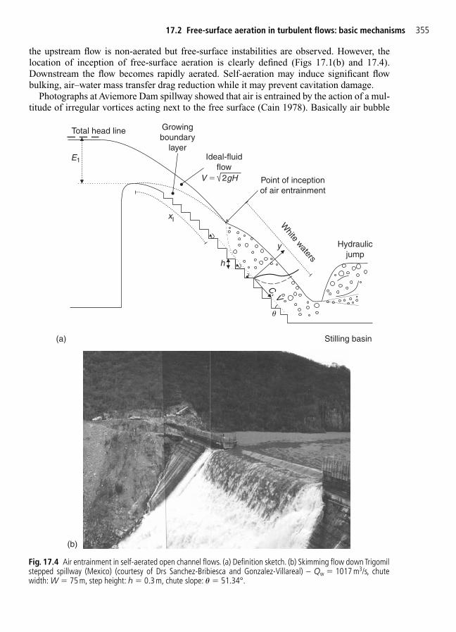
the upstream flow is non-aerated but free-surface instabilities are observed. However, thelocation of inception of free-surface aeration is clearly defined (Figs 17.1(b) and 17.4).Downstream the flow becomes rapidly aerated. Self-aeration may induce significant flowbulking, air–water mass transfer drag reduction while it may prevent cavitation damage.

Photographs at Aviemore Dam spillway showed that air is entrained by the action of a mul-titude of irregular vortices acting next to the free surface (Cain 1978). Basically air bubble

Point of inceptionof air entrainment

White waters

Growingboundary

layer

y

C, V

u

Ideal-fluidflow

V � 2gH

E1

Hydraulicjump

Stilling basin

h

Total head line

xI

(a)

(b)

Fig. 17.4 Air entrainment in self-aerated open channel flows. (a) Definition sketch. (b) Skimming flow down Trigomilstepped spillway (Mexico) (courtesy of Drs Sanchez-Bribiesca and Gonzalez-Villareal) – Qw � 1017 m3/s, chutewidth: W � 75 m, step height: h � 0.3 m, chute slope: � � 51.34°.

17.2 Free-surface aeration in turbulent flows: basic mechanisms 355

356 Interaction between flowing water and free surfaces

entrainment is caused by turbulence fluctuations acting next to the air–water free surface.Through the ‘free surface’, air is continuously trapped and released. Air bubbles may beentrained when the turbulent kinetic energy is large enough to overcome both surface tensionand gravity effects. The turbulent velocity must be greater than the surface tension pressureand the bubble rise velocity component for the bubbles to be carried away:

(17.5)

where V� is an instantaneous turbulent velocity normal to the flow direction, is the surfacetension, �w is the water density, dab is the diameter of the entrained bubble, ur is the bubble risevelocity and � is the channel slope. Equation (17.5) predicts the occurrence of air bubble entrain-ment for V� � 0.1–0.3 m/s. The condition is nearly always achieved in prototype chute flowsbecause of the strong turbulence generated by boundary friction. Interfacial aeration involvesboth the entrainment of air bubbles and the formation of water droplets. The air–water mixtureflow consists of water surrounding air bubbles (C � 30%), air surrounding water droplets(C � 70%) and an intermediate flow structure for 0.3 � C � 0.7 (Fig. 17.2(b)).

V maximum8

cosw ab

r� �

��

du;

Notes1. Relevant monographs on self-aeration in high-velocity chute flows include Falvey

(1980), Wood (1991), Chanson (1997a, 2001b) while specialized publications com-prise Wood (1983), Chanson (1994) and Falvey (1990).

2. Measurements of bubble rise velocity are discussed in Appendix A (Section 3.5) inChapter 3. Typical results are reported in Table 17.1. For millimetric bubbles, the risevelocity of air bubbles in still water is about 0.2–0.4 m/s for 1 � dab � 30 mm.

3. Assuming a rise velocity of 0.25 m/s, equation (17.5) suggests that self-aeration occursfor turbulent velocities normal to the free surface �0.1–0.3 m/s, and bubbles in the range8–40 mm are the most likely to be entrained. For steep slopes the action of the buoyancyforce is reduced and larger bubbles are expected to be carried away. Equation (17.5) isan extension the work of Ervine and Falvey (1987) by Chanson (1993).

4. Rein (1998) and Chanson (1999b) discussed specifically the characteristics of thespray region (i.e. C � 95%).

Table 17.1 Rise velocity of individual air bubblein fresh water and sea water

dab (mm) ur

Fresh water Sea water(1) (2) (3)

0.1 0.0054 0.00450.5 0.135 0.1121 0.402 0.4052 0.297 0.2995 0.238 0.239

10 0.258 0.25920 0.331 0.33230 0.380 0.38050 0.508 0.508

Note: Based upon measured fluid properties reported byChanson et al. (2002).

Downstream of the inception point of free-surface aeration, air and water are fully mixed,forming a homogeneous two-phase flow (Chanson 1995a, 1997a). The advective diffusion ofair bubbles may be described by simple analytical models (Appendix B, Section 17.7). Insmooth-chute flows and in skimming flows over stepped chutes, the air concentration profileshave a S-shape that may be modelled by:

Skimming and smooth-chute flows

where y is distance measured normal to the pseudo-invert, Y90 is the characteristic distancewhere C � 90%, K� is an integration constant and Do is a function of the mean void fractiononly (Appendix B, Section 17.7).

17.2.4 Interfacial aeration process: self-aeration at waterjet interfaces

Turbulent water jets discharging into the atmosphere are often characterized by a substantialamount of free-surface aeration. Applications include water jets at bottom outlets to dissipateenergy, jet flows downstream of a spillway ski jump, mixing devices in chemical plants andspray devices, water jets for fire-fighting, jet cutting (e.g. coal mining) and with Pelton turbines.

C K

yYD

yY

D 1 tanh

132

o o

� � � �

�90 90

3

2 3

5. Note that waves and wavelets propagate downstream along the free surface of super-critical flows. A phase detection probe, fixed in space, will record a fluctuating signalcorresponding to both air–water structures and wave passages, adding complexity ofthe interpretation of the signal (Toombes 2002).

DISCUSSIONOn stepped chutes, low flows behave as a succession of free-falling nappes impacting oneach step (i.e. nappe flow regime). At large discharges, the waters skim over the pseudo-bottom formed by the step edges (i.e. skimming flow regime). For intermediate flowrates, the flow is highly chaotic and aerated (i.e. transition flow regime). In transitionflows down a stepped chute, the distributions of void fraction follow closely:

Transition flows (17.7)

where K� and � are dimensionless function of the mean air content only (Appendix B,Section 17.7).

Although void fraction distribution in transition and skimming flows exhibit differentshapes, equations (17.6) and (17.7) derive from the same basic equation assumingdifferent diffusivity profiles (Appendix B, Section 17.7).

C Ky

Y 1 exp

90

� � � ��

17.2 Free-surface aeration in turbulent flows: basic mechanisms 357

(17.6)

A related case is the ventilated cavity flow, observed downstream of blunt bodies, on theextrados of foils and turbine blades and on spillways (i.e. aeration devices).

Downstream of the jet nozzle, interfacial aeration takes place along the jet interfaces. For atwo-dimensional developing jet flows, the analytical solution of the diffusion equation for airbubble is:

(17.8)

where d1 and V1 are the jet thickness and velocity at the nozzle, x is the streamwise directionand y is the distance normal to the jet centreline (Fig. 17.2, Appendix C, Section 17.8). Forcircular jets, the theoretical solution is significantly more complicated and it is presented inAppendix C (Section 17.8).

DiscussionThere is some similarity between air entrainment in high-velocity water jets and in super-critical open channel flows. (The channel invert is somehow analogue to the jet centreline.)Both flow configurations are high-speed turbulent flows with interfacial aeration rather thanlocal aeration. In water jets and open channel flows, the air bubbles are gradually diffusedand dispersed within the mean flow, and the distributions of air concentrations have a similarS-shape although the characteristics of the shear flow are significantly different.

17.3 Dimensional analysis and similitude

17.3.1 Introduction

Analytical and numerical studies of air–water flows are particularly complex because of the largenumber of relevant equations. Experimental investigations are also difficult but recent advancesin instrumentation brought new measuring systems enabling successful experiments (paragraph17.4). Traditionally model studies are performed with geometrically similar models and the geometric scaling ratio Lr is defined as the ratio of prototype to model dimensions (Fig. 17.5).Laboratory studies of air–water flows require however the selection of an adequate similitude.

17.3.2 Applications

In a study of air–water flows, the relevant parameters needed for any dimensional analysisinclude the fluid properties and physical constants, the channel geometry and inflow conditions,

C

dy

DV

x

12

1 erf

2

1

t

1

� ��

2

358 Interaction between flowing water and free surfaces

Remarks1. Equation (17.8) was first developed by Chanson (1989). It was successfully com-

pared with experimental data by Chanson (1988) and Brattberg et al. (1998).2. Estimates of turbulent diffusivity are discussed in Appendix C (Section 17.8).

(a-i) (a-ii)

(b-i) (b-ii)

Fig. 17.5 Physical modelling of air–water flows. (a) Dropshaft operation (Froude similitude). Left: prototype drop-shaft (3 m high, We � 200). Right: model dropshaft (1 m high, We � 22). (b) Air entrainment at vertical circularplunging jets (Froude similitude) – the probe on the right-hand side gives the scale for the entrained air bubbles. Leftd1 � 12.5 mm, Fr1 � 8.5, We1 � 1500. Right: d1 � 6.83 mm, Fr1 � 8.5, We1 � 370.

360 Interaction between flowing water and free surfaces

the air–water flow properties including the entrained air bubble characteristics, and, possibly,the geometry of the air supply system in closed-conduit systems.

Air entrainment at vertical plunging jetsConsidering the simple steady, vertical, circular plunging jet, a simplified dimensional analy-sis yields a relationship between the air–water flow properties beneath the free surface, the fluidproperties and physical constants, flow geometry, and impingement flow properties:

(17.9)

where C is the void fraction, F is the bubble count rate, V is the velocity, g is the gravity accel-eration, d1 is the jet diameter at impact, u� is a characteristic turbulent velocity, V1 is the jetimpact velocity, dab is a characteristic size of entrained bubble, x is the coordinate in the flowdirection measured from the nozzle, x1 is the free-jet length, r is the radial coordinate, �w and�w are the water density and dynamic viscosity respectively, is the surface tension betweenair and water, u1� is a characteristic turbulent velocity at impingement (Fig. 17.2). In equation(17.9) right-hand side, the fourth and fifth terms are the inflow Froude and Weber numbersrespectively while the seventh term is the Morton number. In addition, biochemical propertiesof the water solution may be considered.

Air entrainment in steep chute flowsConsidering a supercritical flow at uniform equilibrium flows (i.e. normal flow conditions)down a prismatic rectangular channel, a complete dimensional analysis yields:

(17.10a)CV

gd

uV

dd

Fyd

q

gd

q g Wd

kd

, ab2

w

3w

w

w

w

w3

s, , , ; ; ; ; ; ; ;�

�K K��

�

��

4

CFdV

V

gd

uV

dd

Fx x

drd

xd

V

gd

V d uV

g

,

salinity;

1

1 1 1

ab

11

1 1

1

1

1

1

w 12

1

1

w

w

, , , ,

; ; ; ; ; ; ;

�

�� �

1

14

3

K

K�

�

�

Remarks1. Any combination of these numbers is also dimensionless and may be used to replace

one of the combinations. One parameter among the Froude, Reynolds and Weber num-bers can be replaced by the Morton number Mo � g�w

4 /�w3, also called the liquidparameter, since:

The Morton number is a function only of fluid properties and gravity constant. For thesame fluids (air and water) in both model and prototype, Mo is a constant.

2. The bubble count rate F is defined as the number of bubbles detected by the probesensor per second. For a given void fraction and velocity, the bubble count rate is pro-portional to the air–water interface area.

MoWe

Fr Re

3

2 4�

where d is the flow depth at uniform equilibrium, qw is the water discharge per unit width, Wis the channel width, � is the invert slope, ks is the equivalent roughness height, g is the grav-ity acceleration. For air–water flows, the equivalent clear-water depth is defined as:

where y is the distance normal to the invert, C is the local void fraction and Y90 is the depthwhere C � 0.9.

In equation (17.10a) right-hand side, the second, third and fourth dimensionless terms areFroude, Reynolds and Morton numbers respectively, and the last three terms characterize thechute geometry and the skin friction effects on the invert and sidewalls.

Further simplifications may be derived by considering the depth-averaged air–water flowproperties. For a smooth-chute flow at uniform equilibrium, it yields:

(17.10b)

where Uw and d are respectively the mean flow velocity (Uw � qw/d) and equivalent clear-water flow depth at uniform equilibrium flow conditions and Cmean is the depth-averaged voidfraction defined as:

CY

C yy

y Y

mean90 0

1

d��

� 90

∫

FU

gd

U d gC

Wd

kd4

ww

w

w

w

w3 mean

s ; 0; ; ; ; ;��

�

� �

4

�

d C yy

y Y ) d

0� �

�

�(190∫

DISCUSSIONConsidering normal flow conditions down a rectangular stepped channel (horizontalsteps), a dominant flow feature is the momentum exchange between the free stream andthe cavity flow within the steps (Chanson et al. 2002b). Dimensional analysis mustinclude the step cavity characteristics and it yields:

where d is the flow depth at uniform equilibrium, x is the streamwise direction measuredfrom the upstream step edge, h is the step height and ks� the skin roughness height. In theabove equation, the last four terms characterize the step cavity shape and the skin fric-tion effects on the cavity walls.

By considering the depth-averaged air–water flow properties, the above equationbecomes:

where Uw is the mean flow velocity (Uw � qw/d) and Cmean is the depth-averaged voidfraction.

FU

gd

U d gC

dh

Wh

kh5

ww

w

w

w

w3 mean

s ; 0; ; ; ; ; ;�� �

��4 �

�

CV

gd

uV

dd

Fxd

yd

q

gd

q g dh

Wh

kh

, ; ab3

w

3w

w

w

w

w3

s, , , ; ; ; ; ; ; ;�

��

K �� �

�

�4

17.3 Dimensional analysis and similitude 361

362 Interaction between flowing water and free surfaces

17.3.3 Dynamic similarity and scale effects

Despite their simplistic assumptions, equations (17.9) and (17.10a) demonstrate a large num-ber of relevant dimensionless parameters and dynamic similarity of air bubble entrainment atplunging jets and in steep chutes might be impossible with geometrically similar models. Infree-surface flows and wave motion, most laboratory studies are based upon a Froude simili-tude (e.g. Henderson 1966, Hughes 1993, Chanson 1999a) while the entrapment of air bubblesand the mechanisms of air bubble break-up and coalescence are dominated by surface ten-sion effects implying the need for a Weber similitude. For geometrically similar models, it isimpossible to satisfy simultaneously Froude and Weber similarities. In small size models, theair entrainment process may be affected by significant scale effects (Fig. 17.5). Wood (1991)and Chanson (1997a) presented comprehensive reviews. Kobus (1984) illustrated some applications.

Table 17.2 Summary of well-documented scale effects affecting air–water flow studies

Study Similitude Definition of Limiting Experimentalscale effects conditions flow conditions

(1) (2) (3) (4) (5)

Plunging jet flowsChanson Froude Void fraction and bubble We1 � 1 � 103 Vertical circular jets: d1 � 0.05, et al. (2002a), count rate distributions, V1/ur � 10 0.0125, 0.0068 m, 7 � Fr1 � 10Fig. 17.5(b) bubble sizes Lr � 1, 2, 3.66

Stepped chutesBaCaRa (1991) Froudea Flow resistance and Lr � 25 Model studies: � � 53.1°,

energy dissipation h � 0.06, 0.028, 0.024, 0.014 mLr � 10, 21.3, 25, 42.7

Boes (2000) Froudea Void fraction and Re � 1 � 105 Model studies: � � 30° and 50°, velocity distributions W � 0.5 m, h � 0.023–0.093 m

Lr � 6.6, 13, 26 (30°)/6.5, 20 (50°)

Chanson et al. Froudea Flow resistance Re � 1 � 105 Prototype and model studies(2002b) h � 0.02 m � � 5–50°, W � 0.2–15 m,

h � 0.005–0.3 m, 3 � 104 � Re � 2 � 108,10 � We � 6.5 � 106

Gonzalez and Froudea Void fraction, bubble Lr � 2 � � 16°, W � 1 m,Chanson (2004) count rate, velocity h � 0.10, 0.05 m,

and turbulence level 1.2 � 105 � Re � 1.3 � 106

distributions, bubble Lr � 1, 2sizes and clustering

Other studiesSpillway aeration devicePinto and Neidert Froudea Air demand of aerator Lr � 30 Model studies: � � 15°, (1982) W � 0.15 m, 5 � Fr � 17.4

Lr � 8, 15, 30, 50

Dropshaft Chanson (2002b), Froude Bubble penetration Lr � 3.1 Shaft dimensions: 0.76 � 0.76 m2,Fig. 17.5(a) depth and neutrally 0.24 � 0.24 m2, �zo � 1.7 and

buoyant particle 0.55 m, 2 � 103 � Re � 6 � 105

recirculation times Lr � 1, 3.1

Notes: h: step height; Lr: geometric scaling ratio; Re � Vd/�w; W: channel width; We � �wV2d/; �zo: drop in invert elevation;�: chute slope; a: two-dimensional models.

A few studies investigated systematically air–water flows with geometrically similar mod-els under controlled flow conditions (Table 17.2). These were based upon a Froude similitudewith undistorted models and sometimes two-dimensional models. Results are summarized inTable 17.2, Column (4) indicating conditions to avoid scale effects. The outcomes demon-strated that scale effects may be significant. At the limit no scale effect is observed at full scaleonly (Lr � 1) using the same fluids in model and prototype. Basically dynamic similarity ofair entrainment is impossible with geometrically similar models because of too many rele-vant parameters (e.g. equations (17.9) and (17.10a)).

Despite a limited number of systematic studies, results listed in Table 17.2 highlightthe limitations of dynamic similarity and physical modelling of air–water flows. They showfurther that the selection of the criteria to assess scale affects is further critical.

Remarks1. Scale effects are discrepancies between model and prototype resulting when one or

more dimensionless parameters have different values in the model and prototype.2. For a wide channel (e.g. spillway chute), the problem becomes a two-dimensional

study. If the sidewall effects are assumed small, it is often convenient to use a two-dimensional model.

3. The above dimensional considerations were developed for simple flow conditionsand geometries. In real hydraulic structures (e.g. dropshaft, Fig. 17.5(a)), the numberof relevant parameters increases with the complexity of the system.

An example: scale effects on steep stepped chutesFor stepped chutes (Fig. 17.4(b)), several studies demonstrated that a Froude similitudewith geometric similarity and same fluids in model and prototype does not describe thecomplexity of skimming flows. BaCaRa (1991) described a systematic laboratory inves-tigation of the M’Bali Dam spillway with model scales of Lr � 10, 21.3, 25 and 42.7. Forthe smallest models (Lr � 25 and 42.7), the flow resistance was improperly reproduced.Chanson et al. (2002b) re-analysed more than 38 model studies and four prototype inves-tigations with channel slopes ranging from 5.7° up to 55°. They concluded that physicalmodelling of flow resistance may be conducted based upon a Froude similitude if labora-tory flow conditions satisfy h � 0.020 m and Re � 1 � 105. They added that true simi-larity of air entrainment was achieved only for model scales Lr � 10.

However detailed studies of local air–water flow properties yielded more stringentconditions (Table 17.2). One study showed that turbulence levels, entrained bubble sizesand interfacial areas were not properly scaled by a Froude similitude with Lr � 2.

Discussion: fresh water versus salt waterComparative studies of bubble entrainment in fresh water and sea water are scarce (e.g.Scott 1975, Kolaini 1998, Slauenwhite and Johnson 1999). Some studies considered thesize of bubbles produced by a frit, showing that bubble coalescence was drasticallyreduced in salt water compared to freshwater experiments (Lr � 1).

An experimental study in the developing flow region of plunging jets was conductedsystematically with fresh water, sea water and salty fresh water (Chanson et al. 2002b).The results indicated lesser air entrainment in sea water than in fresh water, all inflowparameters being identical (Lr � 1). It was hypothesized that surfactants, biological and

17.3 Dimensional analysis and similitude 363

364 Interaction between flowing water and free surfaces

17.4 Basic metrology in air–water flow studies

17.4.1 Introduction

In hydraulic engineering, most air–water flows are characterized by large amounts of entrainedair. Void fractions are commonly �5–10%, and flows are of high-velocity with ratios of flowvelocity to bubble rise velocity �10 or even 20. Classical measurement devices (e.g. Pitottube, ADV, PIV, LDV) are affected by entrained bubbles and might lead to inaccurate read-ings. When the void fraction C exceeds 5–10%, and is �90–95%, the most robust instrumen-tation is the intrusive phase detection probes: optical fibre probe and conductivity/resistivityprobe. Although the first designs were resistivity probes, both optical fibre and resistivityprobe systems are commonly used today. The intrusive probe is designed to pierce bubbles anddroplets (Fig. 17.6(a)). For example, the probe design shown in Fig. 17.6(a) has a small frontalarea of the first tip to facilitate interface piercing.

The principle behind the optical probe is the change in optical index between the twophases. The principle behind the conductivity, or electrical probe, is the difference in electri-cal resistivity between air and water. The resistance of air is one thousand times larger thanthat of water and a needle resistivity probe gives accurate information on the local void fluc-tuations. A typical probe signal output is shown in Fig. 17.6(b). Although the signal is theo-retically rectangular, the probe response is not exactly square because of the finite size of thetip, the wetting/drying time of the interface covering the tip and the response time of the probeand electronics.

chemical elements harden the induction trumpet and diminish air entrapment atimpingement in sea water. The results implied further that classical dimensional analy-sis is incomplete unless physical, chemical and biological properties other than density,viscosity and surface tension are taken into account.

Notes1. Spillway aeration devices are designed to introduce air into high-velocity flows. Such

aerators include basically a deflector and air is supplied beneath the deflected waters(Vischer et al. 1982, Chanson 1989, 1997a, Falvey 1990). Downstream of the aera-tor, the entrained air can reduce or prevent cavitation erosion.

2. Cavitation is the formation of vapour bubbles within a homogeneous liquid caused byexcessive stress (Franc et al. 1995). Cavitation may occur in low-pressure regionswhere the liquid has been accelerated (e.g. marine propellers, baffle blocks, spillwaychutes). Cavitation modifies the hydraulic characteristics of a system, and it is char-acterized by damaging erosion, additional noise, vibrations and energy dissipation.

3. A dropshaft is a vertical shaft connecting two channels at different invert elevations(Fig. 17.5(a)). The design is commonly used in sewers and stormwater systems. TheRomans built a number of dropshafts along some aqueducts: e.g. Yzeron, Cherchell,Montjeu aqueducts.

4. Sea water is a complex mixture of 96.5% water, 2.5% salts and smaller amounts ofother substances. The most abundant salts are sodium chloride (NaCl), sulphate (SO4),Magnesium (Mg), Calcium (Ca) and Potassium (Riley and Skirrow 1965, OpenUniversity Course Team 1995).

0.1

0.2

0.3

0.4

0.5

0.6

0.7

0.8

0.11 0.112 0.114 0.116 0.118 0.12 0.122 0.124

Leading tipTrailing tip

Time (s)

Voltage

(b)

Fig. 17.6 Local air–water flow measurements in skimming flow down a stepped chute with a double-tip conductiv-ity probe – � � 16°, h � 0.10 m, qw � 0.188 m2/s, dc/h � 1.5, Re � 7.5 � 105, step edge 8, scan rate: 40 kHz persensor for 20 s, Ø � 0.025 mm, �x � 8 mm. (a) Sketch of bubble impact on phase-detection probe tips (dual-tip probedesign). (b) Voltage outputs from a double-tip conductivity probe (y � 39 mm, C � 0.09, V � 3.05 m/s, F � 121 Hz).(c) Normalized auto-correlation and cross-correlation functions (y � 39 mm, C � 0.09, V � 3.05 m/s, F � 121 Hz).

Air bubblechord lengthAir bubble

Water chord

Air chord

Flow direction

∆x

Leading tip

Trailing tip(a)

1

0.9

0.8

0.7

0.6

0.5

0.4

0.3

0.2

0.1

00 0.001

Rxy, Rxx

0.002 0.003 0.004 0.005 0.006 0.007 0.008 0.009Time

Rxy

Rxx

(c)

∆T

∆t

T

17.4 Basic metrology in air–water flow studies 365

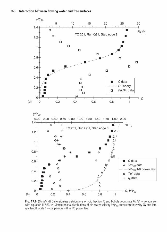
366 Interaction between flowing water and free surfaces

0

0.2

0.4

0.6

0.8

1

1.2

1.4

0 0.2 0.4 0.6 0.8 1

5 10 15 20 25 30

C dataC TheoryFdc/Vc data

y /Y90

C

TC 201, Run Q31, Step edge 8Fdc/Vc

(d)

0

0.2

0.4

0.6

0.8

1

1.2

1.4

0 0.2 0.4 0.6 0.8 1

0.00 0.20 0.40 0.60 0.80 1.00 1.20 1.40 1.60 1.80 2.00

C dataV/V90 dataV/V90 1/6 power law

Tu � dataIL data

y /Y90

C, V/V90

TC 201, Run Q31, Step edge 8Tu, IL

(e)

Fig. 17.6 (Contd ) (d) Dimensionless distributions of void fraction C and bubble count rate Fdc/Vc – comparisonwith equation (17.6). (e) Dimensionless distributions of air–water velocity V/V90, turbulence intensity Tu and inte-gral length scale IL – comparison with a 1/6 power law.

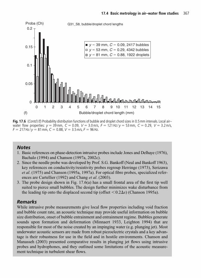
00 1 2 3 4 5 6 7 8 9 10 11 12 13 14 15

0.05

0.1

0.15

0.2

y � 39 mm, C � 0.09, 2417 bubblesy � 53 mm, C � 0.29, 4342 bubblesy � 81 mm, C � 0.88, 1922 droplets

Proba (Ch)

Bubble/droplet chord length (mm)(f)

Q31_S8, bubble/droplet chord lengths

Fig. 17.6 (Contd ) (f) Probability distribution functions of bubble and droplet chord sizes in 0.5 mm intervals. Local air–water flow properties: y � 39 mm, C � 0.09, V � 3.0 m/s, F � 121 Hz / y � 53 mm, C � 0.29, V � 3.2 m/s,F � 217 Hz / y � 81 mm, C � 0.88, V � 3.5 m/s, F � 96 Hz.

Notes1. Basic references on phase-detection intrusive probes include Jones and Delhaye (1976),

Bachalo (1994) and Chanson (1997a, 2002c).2. Since the needle probe was developed by Prof. S.G. Bankoff (Neal and Bankoff 1963),

key references on conductivity/resistivity probes regroup Herringe (1973), Serizawaet al. (1975) and Chanson (1995a, 1997a). For optical fibre probes, specialized refer-ences are Cartellier (1992) and Chang et al. (2003).

3. The probe design shown in Fig. 17.6(a) has a small frontal area of the first tip wellsuited to pierce small bubbles. The design further minimizes wake disturbance fromthe leading tip onto the displaced second tip (offset �0.2�x) (Chanson 1995a).

RemarksWhile intrusive probe measurements give local flow properties including void fractionand bubble count rate, an acoustic technique may provide useful information on bubblesize distribution, onset of bubble entrainment and entrainment regime. Bubbles generatesounds upon formation and deformation (Minnaert 1933, Leighton 1994) that areresponsible for most of the noise created by an impinging water (e.g. plunging jet). Mostunderwater acoustic sensors are made from robust piezoelectric crystals and a key advan-tage is their robustness for use in the field and in hostile environments. Chanson andManasseh (2003) presented comparative results in plunging jet flows using intrusiveprobes and hydrophones, and they outlined some limitations of the acoustic measure-ment technique in turbulent shear flows.

17.4 Basic metrology in air–water flow studies 367

368 Interaction between flowing water and free surfaces

17.4.2 Signal processing and data analysis

The basic probe outputs are the void fraction, bubble count rate and bubble chord time distri-butions with both single-tip and double-tip probe designs. The void fraction C is the propor-tion of time that the probe tip is in the air. The bubble count rate F is the number of bubblesimpacting the probe tip per second. The bubble chord times provide information on theair–water flow structure. For one-dimensional flows, chord sizes distributions may be furtherderived. A dual-tip probe design (Fig. 17.6(a)) provides additionally the air–water velocity,specific interface area, chord length size distributions and turbulence level. This techniqueassumes that the probe tips are aligned along a streamline and that bubbles and droplets arelittle affected by the leading tip.

With a dual-tip probe, the velocity measurement is based upon the successive detection ofair–water interfaces by two sensors. In turbulent air–water flows, the successive detection ofall bubbles by each tip is highly improbable and it is common to use a cross-correlation tech-nique (e.g. Crowe et al. 1998). The time-averaged air–water velocity equals:

(17.11)

where �x is the distance between tips and T is the time for which the cross-correlation func-tion Rxy is maximum (Fig. 17.6(c)). The shape of the cross-correlation function provides fur-ther information on the velocity fluctuations (Chanson and Toombes 2002). The turbulentintensity may be derived from the broadening of the cross-correlation function compared tothe auto-correlation function:

(17.12)

where �T as a time scale satisfying: Rxy(T �T ) � 0.5 Rxy(T ), Rxy is the normalized cross-correlation function, and �t is the characteristic time for which the normalized auto-correlationfunction Rxx equals 0.5 (Fig. 17.6(c)). The auto-correlation function Rxx provides some infor-mation on the air–water flow structure. A dimensionless integral length scale is:

(17.13)

Figure 17.6(d) and (e) presents some example of void fraction, bubble count rate, velocityand turbulence intensity distributions measured in a skimming flow down a stepped cascade.All data presented in Fig. 17.6 were recorded at the same cross-section. (Details are given inChanson and Toombes 2002.)

A time-series analysis gives information on the frequency distribution of the signal whichis related to the air and water (or water and air) length scale distribution of the flow. Chordsizes may be calculated from the raw probe signal outputs. The results provide a completecharacterization of the streamwise distribution of air and water chords, including the exis-tence of bubble/droplet clusters. Figure 17.6(f) presents probability distribution functions ofbubble and droplet chord sizes in 0.5 mm intervals. Bubble chord sizes are indicated in whiteand black, while droplet chord sizes in grey. Data for chord sizes exceeding 15 mm were notshown for clarity.

It

TL 0.851��

TuuV

T tT

0.851 2 2

��

�� � �

Vx

T �

�

The measurement of air–water interface area is a function of void fraction, velocity and bub-ble sizes. The specific air–water interface area a is defined as the air–water interface area perunit volume of air and water. For any bubble shape, bubble size distribution and chord lengthdistribution, it may be derived from continuity:

(17.14)

where equation (17.14) is valid in bubbly flows (C � 0.3). In high air content regions, theflow structure is more complex and the specific interface area a becomes simply proportionalto the number of air–water interfaces per unit length of flow (a � 2F/V).

With relative ease, intrusive phase-detection probes may provide detailed information on bubble count rate, specific interface area and bubble chord sizes. Such information isessential to gain a better understanding of air–water mass transfer in hydraulic engineeringapplications. It further assists comprehension of the interactions between turbulence andentrained air.

aF

V

4�

Remarks1. A dual-tip probe provides only streamwise measurements. It does not give informa-

tion on transverse flow properties.2. The signal output analysis is basically identical for conductivity and optical fibre

probes.3. In turbulent shear flows, bubble size distributions are possibly best fitted by a log-normal

distribution, although both Gamma and Weibull distributions provided also good fit.Basic experimental results include Cummings and Chanson (1997b) and Chanson et al. (2002a) in the developing flow region of vertical plunging jets, Chanson (1997b)in smooth-chute flows, Chanson and Toombes (2002) in skimming flow on steppedchute and Brattberg et al. (1998) in high-velocity jets.

4. The streamwise distribution of bubbles provides information on their spatial arrange-ment and the existence of bubble cluster. In a cluster, the bubbles are close togetherand the packet is surrounded by a sizeable volume of water. The existence of bubbleclusters may be related to break-up, coalescence, bubble wake interference and toother processes. As the bubble response time is significantly smaller than the charac-teristic time of the flow, bubble trapping in large-scale turbulent structures may alsobe a clustering mechanism in bubbly flows. Preliminary studies include Chanson andToombes (2002).

Discussion: Velocity measurements in air–water flowsSome studies suggested that interfacial velocities may be measured with a single-tipphase-detection probe based upon the voltage rise time associated with a water–air tran-sition. This technique is, however, restricted to specific applications and probe designs.It was believed that the drying process on the probe sensor is strongly affected by thepresence of water impurities and by sensor shape irregularities, yielding a wide scatter

17.4 Basic metrology in air–water flow studies 369

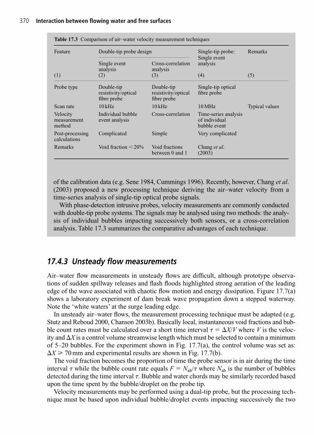
370 Interaction between flowing water and free surfaces

17.4.3 Unsteady flow measurements

Air–water flow measurements in unsteady flows are difficult, although prototype observa-tions of sudden spillway releases and flash floods highlighted strong aeration of the leadingedge of the wave associated with chaotic flow motion and energy dissipation. Figure 17.7(a)shows a laboratory experiment of dam break wave propagation down a stepped waterway.Note the ‘white waters’ at the surge leading edge.

In unsteady air–water flows, the measurement processing technique must be adapted (e.g.Stutz and Reboud 2000, Chanson 2003b). Basically local, instantaneous void fractions and bub-ble count rates must be calculated over a short time interval � � �X/V where V is the veloc-ity and �X is a control volume streamwise length which must be selected to contain a minimumof 5–20 bubbles. For the experiment shown in Fig. 17.7(a), the control volume was set as:�X � 70 mm and experimental results are shown in Fig. 17.7(b).

The void fraction becomes the proportion of time the probe sensor is in air during the timeinterval � while the bubble count rate equals F � Nab/� where Nab is the number of bubblesdetected during the time interval �. Bubble and water chords may be similarly recorded basedupon the time spent by the bubble/droplet on the probe tip.

Velocity measurements may be performed using a dual-tip probe, but the processing tech-nique must be based upon individual bubble/droplet events impacting successively the two

of the calibration data (e.g. Sene 1984, Cummings 1996). Recently, however, Chang et al.(2003) proposed a new processing technique deriving the air–water velocity from atime-series analysis of single-tip optical probe signals.

With phase-detection intrusive probes, velocity measurements are commonly conductedwith double-tip probe systems. The signals may be analysed using two methods: the analy-sis of individual bubbles impacting successively both sensors, or a cross-correlationanalysis. Table 17.3 summarizes the comparative advantages of each technique.

Table 17.3 Comparison of air–water velocity measurement techniques

Feature Double-tip probe design Single-tip probe: Remarks

Single event Cross-correlation Single event

analysis analysis analysis

(1) (2) (3) (4) (5)

Probe type Double-tip Double-tip Single-tip optical resistivity/optical resistivity/optical fibre probefibre probe fibre probe

Scan rate 10 kHz 10 kHz 10 MHz Typical values

Velocity Individual bubble Cross-correlation Time-series analysis measurement event analysis of individualmethod bubble event

Post-processing Complicated Simple Very complicatedcalculations

Remarks Void fraction �20% Void fractions Chang et al. between 0 and 1 (2003)

(a)

00 0.2 0.4 0.6 0.8 1

0.05

0.1

0.15

0.2

0.25

0.3

0–70 mm

Theory(0–210 mm)

C

y /do

UQ 3.4° slope, h � 0.07 m

Q � 75 L/s, step 16, x � � 0.8 m

0–210 mm0–385 mm350–735 mm700–1085 mmSteady flowTheory steadyflow

Theory(700–1085 mm)

Theory(350–735 mm)

Theory(0–385 mm)

(b)

(mm) 0–70 0–210 0–385 350–735 700–1085 2100–2485 4200–4585

�X (m) 0.070 0.210 0.385 0.385 0.385 0.385 0.385(t � ts) ��g/do� 0.0828 0.248 0.455 1.283 2.110 5.421 10.39Cmean 0.77 0.43 0.46 0.35 0.31 0.24 0.22

Fig. 17.7 (Contd )

372 Interaction between flowing water and free surfaces

0

10

20

30

40

50

60

0.00 1.00 2.00 3.00 4.00 5.00 6.00 7.00 8.00

y (mm)

V (m/s)

x � � 1.0 m, first interface (t � 0.12 s)

Theory

x ��1.0 m, first interface

(c)

Tu � Std(V )/V

y (mm)0 0.2 0.4 0.6 0.8 1 1.2 1.4

0

10

20

30

40

50

60

0.00 1.00 2.00 3.00 4.00 5.00 6.00(d)V (m/s)

Turbulence intensity

Mean velocity

x � � 1.0 m, mean value over all recording

Fig. 17.7 (Contd ) Unsteady air–water flow measurements in the leading edge of dam break wave. (a) Advancingflood waves down stepped chute – looking upstream at an advancing wave on step 16 with an array of conductiv-ity probes in foreground – Q(t � 0) � 0.055 m3/s, do � 0.241 m, 3.4° slope, h � 0.07 m (W � 0.5 m). (b)Dimensionless void fraction distributions in dam break wave front – Step 16, Q(t � 0) � 0.075 m3/s, x� � 0.8 m –comparison with steady flow data and with equations (17.6) and (17.7) – refer table in Fig. b. (c) Interfacial velocitydistribution of the first air-to-water interface (t � 0.12 s) – comparison with the first Stokes problem solution – Step16, Q (t � 0) � 0.065 m3/s, x� � 1 m. (d) Median interfacial velocity and average turbulence intensity (over about5 s) in the dam break wave front – Step 16, Q(t � 0) � 0.065 m3/s, x� � 1 m.

probe sensors. The velocity is deduced from the time lag for air–water interface detectionsbetween leading and trailing tips respectively. For each meaningful event, the interfacialvelocity is calculated as: V � �x/�t where �x is the distance between probe sensors and �t isthe interface travelling time between probe sensors.

An example: Air entrainment in dam break wave frontTypical unsteady void fraction distributions are presented in Fig. 17.7(b) for a dam breakwave (Fig. 17.7(a)). In Fig. 17.7(b), the legend indicates the location and size of the con-trol volume behind the leading edge of wave front: e.g. 350–735 mm means a 385 mmlong control volume located between 350 and 735 mm behind the leading edge. Voidfraction data are plotted as functions of the dimensionless distance y/do, where y is thedistance normal to the invert and do is a measure of the surging flow rate Q(t � 0):

where W is the channel width. In Fig. 17.7(b), the data are compared with the corre-sponding steady flow data while the depth-averaged void fraction Cmean is given in thefigure caption. In steady flow, the mean air content was Cmean � 0.24.

For the same type of experiment, typical air–water velocity measurements are shownin Fig. 17.7(c) and (d). In Fig. 17.7(c), each data point represents the velocity of the firstair-to-water interface at each location y. Figure 17.7(d) presents the mean velocity andthe ratio of interfacial velocity standard deviation to mean velocity for the first 5 s of theflow. (For large interface counts, the ratio is the turbulence intensity Tu.) At the leadingedge of dam break wave, instantaneous velocity measurements suggest a boundary layerregion with a potential region above (Fig. 17.7(c)). Boundary layer velocity data werecompared successfully with an analytical solution of the Navier–Stokes equations (firstStokes problem):

where U is the free-stream velocity, �T is the kinematic viscosity, t is the time from thefirst water detection by a reference probe and y is the distance normal to the invert. Erfis the Gaussian error function defined as:

Figure 17.7(d) highlight high levels of turbulence in the surging flow that are consistentwith steady air–water flow measurements in stepped chutes (Chanson and Toombes 2002).

erf( ) 2

exp d2u z zu

� �� 0∫

( )

VU

y

t erf

2 T

��

dQ t

gWo

2

2

94

( 0 )�

� 3

17.5 Applications

17.5.1 Application to plunging jet flows

General considerationsAt a plunging jet, air entrainment takes place when the jet impact velocity V1 exceeds a crit-ical threshold, called onset or inception velocity. For rough turbulent jet flows, the inception

17.5 Applications 373

374 Interaction between flowing water and free surfaces

velocity Ve is about 1 m/s for a vertical jet discharging into fresh water and sea water (para-graph 17.2.2). Ve tends to decrease slightly with decreasing angle � between the jet flowdirection and the pool free surface, but it should tend to the onset velocity of air entrainmentat hydraulic jumps (Ve � 1 m/s) for � � 0.

For plunging jet velocities greater than the onset velocity, air entrainment takes place. Theair entrainment rate is often expressed as:

(17.15)

where Qair is the entrained air discharge, Qw is the plunging jet flow rate, and d1 and V1 arerespectively the jet thickness/diameter and velocity at impact. Some results are detailed inAppendix A (Section 17.6). It is important, however, to note that most results were obtainedin deep receiving pool with no or slow transverse flow motion in the receiving pool. Somestudies suggested a decrease in air entrainment rate with decreasing pool depth.

Beneath the entrapment point, the bubbly flow consists of a downward plume surroundedby a swarm of rising bubbles. In the downward flow region, the ‘diffusion cone’ consists adeveloping flow region, a redistribution zone and a fully developed flow region (Fig. 17.8).In the developing air–water flow region, the air content is zero on the jet centreline and thevelocity is the ideal-fluid flow velocity. The air diffusion layer and the momentum shear layer

QQ

FV V

gdair

w

1 e

1

��

V1

Developingair diffusion

layer

Fully developedair diffusion

layer

Developingflow region

Fully developedflow region

Developingshearlayer

Fullydeveloped

shearflow

Redistributionzone

C

V

V

d1

C

Fig. 17.8 Schematic of air–water flow region at a plunging jet (after Chanson 1997a).

are developing, and there is some momentum transfer from the jet core to the surroundingliquid. The entrained bubbles are advected in regions of high shear stresses and they are bro-ken up into bubbles of smaller sizes. Downstream of the location where the developing airdiffusion layers meet, the air content is rapidly redistributed from zero air concentration tomaximum void fraction on the centreline. Experimental evidences showed that the develop-ing shear layers and air diffusion layers do not intersect of the same location as sketched inFig. 17.8. Further downstream, both void fraction and velocity distributions are fully devel-oped. The air content and velocity are maximum on the jet centreline. The jet velocity decayswith streamwise distance as fluid is entrained and momentum is exchanged with the pool.

In the surrounding swarm of rising bubbles, the flow motion is driven by buoyancy, althoughit is strongly affected by large-scale vortical structures. Several researchers observed that finebubbles could be trapped in large eddies for a substantial time, while one study noted sub-merged air bubbles more than 5 min after stopping the plunging jet (Chanson et al. 2002a).

DiscussionA related application is the analysis of experimental observations performed with phase-detection intrusive probes. Two examples are discussed below.

Case no. 1: Air–water flow measurements in circular plunging jet flowExperiments were conducted with a circular jet discharging vertically into a seawater pool.The nozzle (12.5 mm diameter) was located 0.05 m above the pool free surface and the flow ratewas 0.394 L/s. Void fraction measurements beneath the pool free surface are reported below.Estimate the dimensionless air flow rate and bubble diffusivity.

Remarks1. Basic reviews on air entrainment at plunging jets include Bin (1993) and Chanson

(1997a).2. A theoretical value of the maximum bubble penetration depth Dp can be deduced

from the continuity and momentum equations for diffusing jets:

Two-dimensional jet

Circular jet

where Dp is the penetration depth measured normal to the pool free surface, d1 and V1are the jet thickness and velocity at impact, ur is the bubble rise velocity, � is the jetimpact angle with the receiving pool of water and �3 is the outer spread angle in thefully developed flow region. For circular jets, �3 � 14° on models and prototypes.

The above equations are based upon the method of Ervine and Falvey (1987)extended by Chanson and Cummings (1992).

D

d

V

u

u

V

u

V

p

1 0.040

r

sin1 12.5 r tan

sin 1 25 r tan1

2

1 1

� � �

�

�

�

�

�

�tan sin3

3 3

D

d

V

u

u

V

p

1 0.0240 1

r

(sin )1 1 20.81 r

1

tan3

� �

2

32

2

32

2

�

�

�

�(tan ) (sin )

17.5 Applications 375

376 Interaction between flowing water and free surfaces

First the inflow conditions must be calculated. The impingement velocity V1 is calculatedusing the Bernoulli principle:

Bernoulli principle

where x1 is the free-jet length (x1 � 0.05 m) and Vn is the nozzle velocity. The jet diameter atimpact is deduced from the continuity equation: Qw � V1(�/4)d1

2. It yields: V1 � 3.36 m/sand d1 � 0.0122 m.

Then the void fraction distributions may be compared with the analytical solution of theadvective diffusion equation for bubbles (equation (17.4)). In practice, however, the data arebest fitted by:

(17.16)

where ro is an arbitrary location slightly greater than the jet radius at impingement (i.e.ro � d1/2).

CQQ

Dx x

rD

rr

x xr

ID

rr

x xr

1

4

exp

1

air

w # 1

o

#o

1

o

o #o

1

o

��

�

� �

1

4

1

2

2

V V gx1 2n2

1�

x � x1 � 10 mm x � x1 � 25 mm

y (cm) C (%) y (cm) C (%) y (cm) C (%) y (cm) C (%)

34.62 1.55 36.6 11.785 34.5 1.48 35.46 0.4834.65 1.61 36.63 9.17 34.53 1.2 36.16 0.7734.68 2.47 36.66 6.255 34.56 1.47 36.19 1.8334.71 2.23 36.69 3.775 34.59 2.02 36.22 3.7834.74 2.58 36.72 4.34 34.62 2.325 36.25 1.70534.77 3.98 36.75 2.74 34.65 2.655 36.28 2.39534.8 5.84 36.78 1.49 34.68 2.625 36.31 2.60534.83 7.16 36.81 1.345 34.71 3.145 36.34 3.44534.86 8.47 34.74 3.32 36.37 4.0134.89 9.72 34.77 4.425 36.4 5.39534.92 11.82 34.8 6.87 36.43 734.95 18.00 34.83 6.605 36.46 9.83534.98 19.22 34.86 6.62 36.49 11.23535.01 21.36 34.89 6.99 36.52 14.0435.04 26.23 34.92 9.58 36.55 16.63535.07 23.17 34.95 10.685 36.58 16.8635.1 25.36 34.98 11.515 36.61 16.8235.13 19.77 35.01 12.805 36.64 15.8135.16 12.33 35.04 13 36.67 14.4635.19 4.27 35.07 12.25 36.7 10.72535.22 1.61 35.1 10.84 36.73 13.0135.25 0.87 35.13 10.295 36.76 8.7136.3 1.59 35.16 8.615 36.79 8.5136.33 3.59 35.19 7.66 36.82 5.96536.36 6.38 35.22 6.025 36.85 2.86536.39 13.43 35.25 4.23 36.88 2.86536.42 18.84 35.28 2.715 36.91 2.0436.45 21.20 35.31 2.175 36.94 1.4536.48 23.63 35.34 1.98 36.97 1.14536.51 20.56 35.37 1.45 37 0.64536.54 17.15 35.4 0.925 37.03 0.5136.57 12.67 35.43 0.77

Note: Data by Chanson et al. (2002a), Run Sea_6.

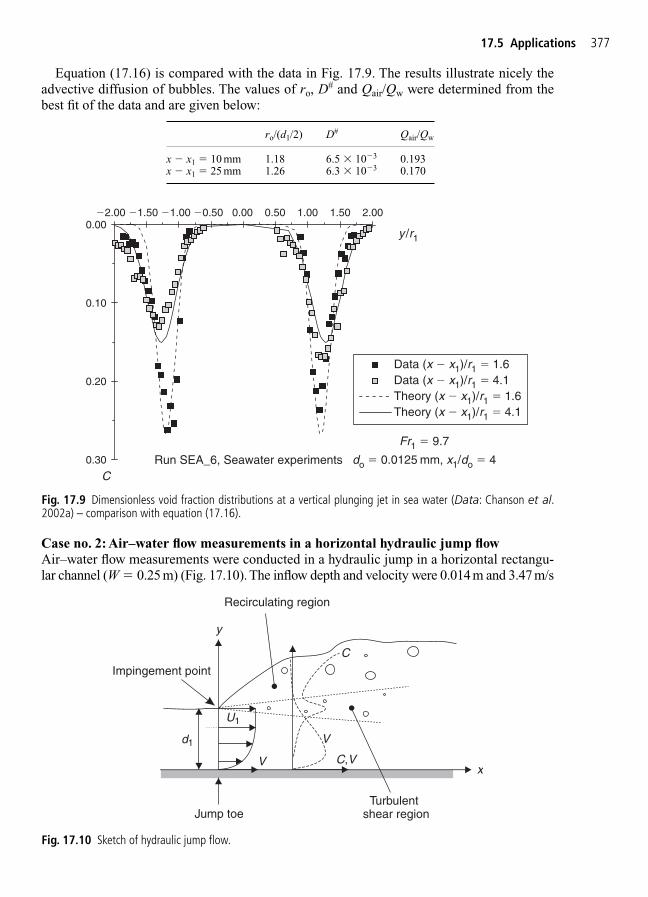
Equation (17.16) is compared with the data in Fig. 17.9. The results illustrate nicely theadvective diffusion of bubbles. The values of ro, D

# and Qair/Qw were determined from thebest fit of the data and are given below:

ro/(d1/2) D# Qair/Qw

x � x1 � 10 mm 1.18 6.5 � 10�3 0.193x � x1 � 25 mm 1.26 6.3 � 10�3 0.170

y

Jump toe

d1

Turbulentshear region

Recirculating region

Impingement point

xV

U1

C

V

C,V

Fig. 17.10 Sketch of hydraulic jump flow.

0.00

0.10

0.20

0.30

�2.00 �1.50 �1.00 �0.50 0.00 0.50 1.00 1.50 2.00

Data (x � x1)/r1 � 1.6Data (x � x1)/r1 � 4.1Theory (x � x1)/r1 � 1.6Theory (x � x1)/r1 � 4.1

y /r1

CRun SEA_6, Seawater experiments

Fr1 � 9.7

do � 0.0125 mm, x1/do � 4

Fig. 17.9 Dimensionless void fraction distributions at a vertical plunging jet in sea water (Data: Chanson et al.2002a) – comparison with equation (17.16).

17.5 Applications 377

Case no. 2: Air–water flow measurements in a horizontal hydraulic jump flowAir–water flow measurements were conducted in a hydraulic jump in a horizontal rectangu-lar channel (W � 0.25 m) (Fig. 17.10). The inflow depth and velocity were 0.014 m and 3.47 m/s

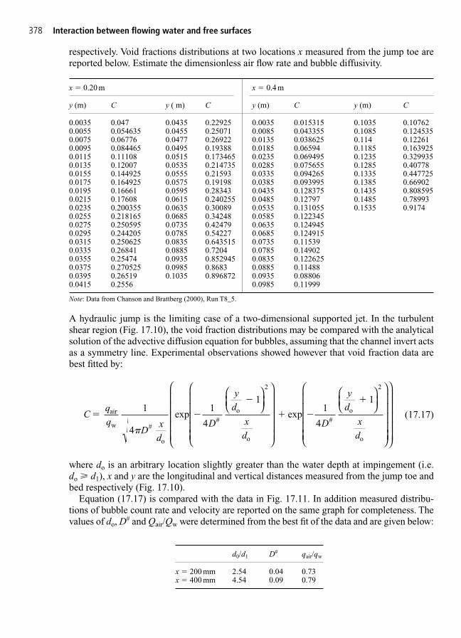
respectively. Void fractions distributions at two locations x measured from the jump toe arereported below. Estimate the dimensionless air flow rate and bubble diffusivity.

A hydraulic jump is the limiting case of a two-dimensional supported jet. In the turbulentshear region (Fig. 17.10), the void fraction distributions may be compared with the analyticalsolution of the advective diffusion equation for bubbles, assuming that the channel invert actsas a symmetry line. Experimental observations showed however that void fraction data arebest fitted by:

where do is an arbitrary location slightly greater than the water depth at impingement (i.e.do � d1), x and y are the longitudinal and vertical distances measured from the jump toe andbed respectively (Fig. 17.10).

Equation (17.17) is compared with the data in Fig. 17.11. In addition measured distribu-tions of bubble count rate and velocity are reported on the same graph for completeness. Thevalues of do, D

# and Qair/Qw were determined from the best fit of the data and are given below:

Cqq

Dx

d

D

yd

xd

D

yd

xd

1

4

exp

1

exp

1air

w #

o

#o

o

#o

o

� �

�

�

�

1

4

1

4

2 2

x � 0.20 m x � 0.4 m

y (m) C y ( m) C y (m) C y (m) C

0.0035 0.047 0.0435 0.22925 0.0035 0.015315 0.1035 0.107620.0055 0.054635 0.0455 0.25071 0.0085 0.043355 0.1085 0.1245350.0075 0.06776 0.0477 0.26922 0.0135 0.038625 0.114 0.122610.0095 0.084465 0.0495 0.19388 0.0185 0.06594 0.1185 0.1639250.0115 0.11108 0.0515 0.173465 0.0235 0.069495 0.1235 0.3299350.0135 0.12007 0.0535 0.214735 0.0285 0.075655 0.1285 0.407780.0155 0.144925 0.0555 0.21593 0.0335 0.094265 0.1335 0.4477250.0175 0.164925 0.0575 0.19198 0.0385 0.093995 0.1385 0.669020.0195 0.16661 0.0595 0.28343 0.0435 0.128375 0.1435 0.8085950.0215 0.17608 0.0615 0.240255 0.0485 0.12797 0.1485 0.789930.0235 0.200355 0.0635 0.30089 0.0535 0.131055 0.1535 0.91740.0255 0.218165 0.0685 0.34248 0.0585 0.1223450.0275 0.250595 0.0735 0.42479 0.0635 0.1249450.0295 0.244205 0.0785 0.54227 0.0685 0.1249150.0315 0.250625 0.0835 0.643515 0.0735 0.115390.0335 0.26841 0.0885 0.7204 0.0785 0.149020.0355 0.25474 0.0935 0.852945 0.0835 0.1226250.0375 0.270525 0.0985 0.8683 0.0885 0.114880.0395 0.26519 0.1035 0.896872 0.0935 0.088060.0415 0.2556 0.0985 0.11999

Note: Data from Chanson and Brattberg (2000), Run T8_5.

378 Interaction between flowing water and free surfaces

d0/d1 D# qair/qw

x � 200 mm 2.54 0.04 0.73x � 400 mm 4.54 0.09 0.79

(17.17)

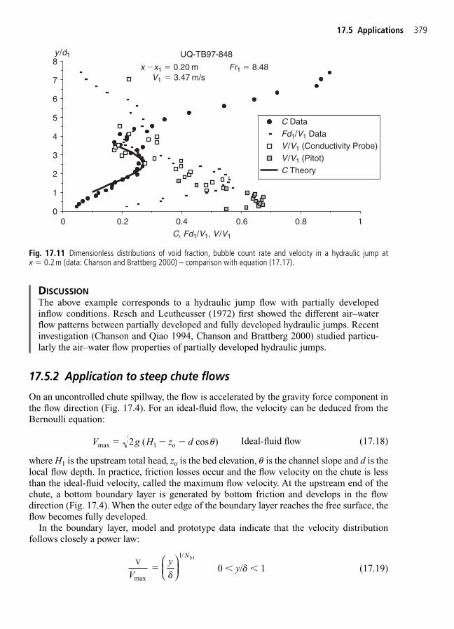
17.5.2 Application to steep chute flows

On an uncontrolled chute spillway, the flow is accelerated by the gravity force component inthe flow direction (Fig. 17.4). For an ideal-fluid flow, the velocity can be deduced from theBernoulli equation:

Ideal-fluid flow (17.18)

where H1 is the upstream total head, zo is the bed elevation, � is the channel slope and d is thelocal flow depth. In practice, friction losses occur and the flow velocity on the chute is lessthan the ideal-fluid velocity, called the maximum flow velocity. At the upstream end of thechute, a bottom boundary layer is generated by bottom friction and develops in the flowdirection (Fig. 17.4). When the outer edge of the boundary layer reaches the free surface, theflow becomes fully developed.

In the boundary layer, model and prototype data indicate that the velocity distribution follows closely a power law:

0 � y/ � 1 (17.19)V

max

b1

Vy

N

�

1/

V g H z dmax 1 o 2 ( cos )� � � �

0

1

2

3

4

5

6

7

8

0 0.2 0.4 0.6 0.8 1

C Data

Fd1/V1 Data

V /V1 (Conductivity Probe)

V /V1 (Pitot)

C Theory

y /d1

Fr1 � 8.48

UQ-TB97-848

x �x1 � 0.20 m V1 � 3.47 m/s

C, Fd1/V1, V /V1

Fig. 17.11 Dimensionless distributions of void fraction, bubble count rate and velocity in a hydraulic jump atx � 0.2 m (data: Chanson and Brattberg 2000) – comparison with equation (17.17).

DISCUSSIONThe above example corresponds to a hydraulic jump flow with partially developedinflow conditions. Resch and Leutheusser (1972) first showed the different air–waterflow patterns between partially developed and fully developed hydraulic jumps. Recentinvestigation (Chanson and Qiao 1994, Chanson and Brattberg 2000) studied particu-larly the air–water flow properties of partially developed hydraulic jumps.

17.5 Applications 379

where is the boundary layer thickness defined as � y(V � 0.99 � Vmax) and y is the distance normal to the channel bed. The velocity distribution exponent equals typicallyNbl � 6 for smooth concrete chutes. For smooth inverts, the boundary growth may be estimated as:

Smooth concrete chute (� � 30°) (17.20)

where x is the distance from the crest measured along the chute invert, � is the chute slopeand ks is the equivalent roughness height. Equation (17.20) is a semi-empirical formulawhich fits well model and prototype data (Wood et al. 1983, Chanson 1997). For steppedchutes with skimming flow, the turbulence generated by the steps enhances the boundarylayer growth. The following formula can be used in first approximation:

Stepped chute (skimming flow) (17.21)

where h is the step height. Equation (17.21) was checked with model and prototype data(Chanson 2001b). It applies only to skimming flow on steep chutes (i.e. � � 30°).

Free-surface aeration takes place downstream of the intersection of the outer edge of thedeveloping boundary layer with the free surface. Air entrainment is clearly identified by the‘white water’ appearance of the free-surface flow (e.g. Fig. 17.4). For smooth inverts, the flowproperties at the inception of free-surface aeration may be estimated as:

Smooth chute (17.22)

Smooth chute (17.23)

where xI and dI are the distance and flow depth respectively at the intersection of the bound-ary layer outer edge with the free surface, F* � qw/�g sin �ks

3, qw is the discharge per unitwidth, g is the gravity constant, ks is the roughness height and � is the channel slope. Forstepped channel the characteristics of the inception of free-surface aeration are best esti-mated as:

Stepped chute (17.24)

Stepped chute (17.25)

where F* is now the Froude number defined in terms of the step roughness height:F* � qw/��g sin� ��(h�co�s ���)3� and h cos � is the step roughness height.

dh

FI0.04

0.592

cos

0.4034

(sin )( )

� �� *

xh

FI 0.0796 0.713

cos 9.719 (sin ) ( )

��� *

dk

FI

s0.04

0.643 0.223

(sin )( )�

�*

xk

FI

s

0.0796 0.713 13.6 (sin ) ( )� � *

�

�xx

h 0.06106 (sin )

cos0.133�

�

0 17.

�

xxk

0.0212 (sin )0.11

s

�

�

0 10.

380 Interaction between flowing water and free surfaces

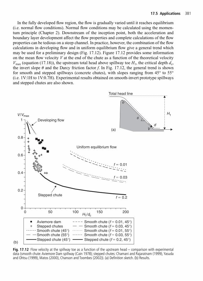
In the fully developed flow region, the flow is gradually varied until it reaches equilibrium(i.e. normal flow conditions). Normal flow conditions may be calculated using the momen-tum principle (Chapter 2). Downstream of the inception point, both the acceleration andboundary layer development affect the flow properties and complete calculations of the flowproperties can be tedious on a steep channel. In practice, however, the combination of the flowcalculations in developing flow and in uniform equilibrium flow give a general trend whichmay be used for a preliminary design (Fig. 17.12). Figure 17.12 provides some informationon the mean flow velocity V at the end of the chute as a function of the theoretical velocityVmax (equation (17.18)), the upstream total head above spillway toe H1, the critical depth dc,the invert slope � and the Darcy friction factor f. In Fig. 17.12, the general trend is shownfor smooth and stepped spillways (concrete chutes), with slopes ranging from 45° to 55°(i.e. 1V:1H to 1V:0.7H). Experimental results obtained on smooth-invert prototype spillwaysand stepped chutes are also shown.

Aviemore damStepped chutesSmooth chute (45°)Smooth chute (55°)Stepped chute (45°)

Smooth chute (f � 0.01, 45°)Smooth chute (f � 0.03, 45°)Smooth chute (f � 0.01, 55°)Smooth chute (f � 0.03, 55°)Stepped chute (f � 0.2, 45°)

0

0.2

0.4

0.6

0.8

1

(b)

V /Vmax

0 50 100 150 200H1/dc

f � 0.01

f � 0.03

f � 0.2

Uniform equilibrium flow

Developing flow

Stepped chute

x

o

H1

Total head line

u

dV(a)

Fig. 17.12 Flow velocity at the spillway toe as a function of the upstream head – comparison with experimentaldata (smooth chute: Aviemore Dam spillway (Cain 1978); stepped chutes: Chamani and Rajaratnam (1999), Yasudaand Ohtsu (1999), Matos (2000), Chanson and Toombes (2002)). (a) Definition sketch. (b) Results.

17.5 Applications 381

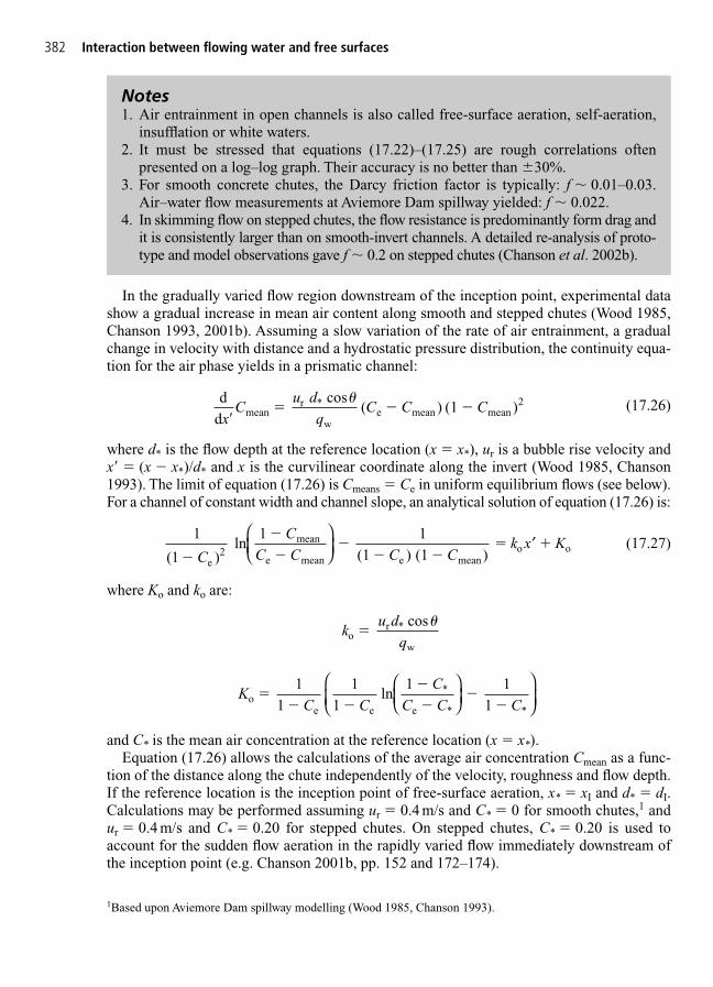
382 Interaction between flowing water and free surfaces

In the gradually varied flow region downstream of the inception point, experimental datashow a gradual increase in mean air content along smooth and stepped chutes (Wood 1985,Chanson 1993, 2001b). Assuming a slow variation of the rate of air entrainment, a gradualchange in velocity with distance and a hydrostatic pressure distribution, the continuity equa-tion for the air phase yields in a prismatic channel:

(17.26)

where d* is the flow depth at the reference location (x � x*), ur is a bubble rise velocity andx� � (x � x*)/d* and x is the curvilinear coordinate along the invert (Wood 1985, Chanson1993). The limit of equation (17.26) is Cmeans � Ce in uniform equilibrium flows (see below).For a channel of constant width and channel slope, an analytical solution of equation (17.26) is:

(17.27)

where Ko and ko are:

and C* is the mean air concentration at the reference location (x � x*).Equation (17.26) allows the calculations of the average air concentration Cmean as a func-

tion of the distance along the chute independently of the velocity, roughness and flow depth.If the reference location is the inception point of free-surface aeration, x* � xI and d* � dI.Calculations may be performed assuming ur � 0.4 m/s and C* � 0 for smooth chutes,1 andur � 0.4 m/s and C* � 0.20 for stepped chutes. On stepped chutes, C* � 0.20 is used toaccount for the sudden flow aeration in the rapidly varied flow immediately downstream ofthe inception point (e.g. Chanson 2001b, pp. 152 and 172–174).

KC C

CC C Co

e e

*

e * *

1

1 1

1 ln

1

1

1 �

� �

�

��

�

ku d

qor *

w

cos

��

1

1 2( ) ) ) ln

1

1

(1 (1

e

mean

e mean e meano o

�

�

��

� ��

C

CC C C C

k x K

′

dd

cos

( ) (1 )meanr *

we mean mean

2

xC

u dq

C C C�

� � ��

Notes1. Air entrainment in open channels is also called free-surface aeration, self-aeration,

insufflation or white waters.2. It must be stressed that equations (17.22)–(17.25) are rough correlations often

presented on a log–log graph. Their accuracy is no better than �30%.3. For smooth concrete chutes, the Darcy friction factor is typically: f � 0.01–0.03.

Air–water flow measurements at Aviemore Dam spillway yielded: f � 0.022.4. In skimming flow on stepped chutes, the flow resistance is predominantly form drag and

it is consistently larger than on smooth-invert channels. A detailed re-analysis of proto-type and model observations gave f � 0.2 on stepped chutes (Chanson et al. 2002b).

1Based upon Aviemore Dam spillway modelling (Wood 1985, Chanson 1993).

Drag reduction in self-aerated chute flowsAir–water flow measurements show smooth, continuous distributions of air concentrations andair–water velocity in smooth and stepped chutes. Although the presence of air bubbles does notaffect the velocity profile, experimental observations demonstrate some drag reduction whichincreases with the mean air concentration Cmean (Fig. 17.13) (Wood 1983, Chanson 1994,2004a, b).

On smooth-invert chutes, the presence of air reduces the shear stress between flow layers.An estimate of the drag reduction is:

(17.28)

where tanh is the hyperbolic tangent function, fe is the air–water flow friction factor and f is thenon-aerated flow friction factor. Equation (17.28) characterizes the reduction in skin friction

ff

CC C

e mean

mean mean

0.5 1 tanh 0.6280.514

(1 )�

�

�

Remark: Uniform equilibrium air content on steep chutesFar downstream, at uniform equilibrium, the depth-averaged void fraction Cmean tends toa constant Ce function of the channel slope � only on smooth and stepped inverts.Uniform equilibrium air content data are shown in Table 17.4. The results are valid forboth smooth and stepped chutes (Wood 1983, Chanson 1997a, 2001). For slopes �50°,the equilibrium mean air concentration may be approximated by: Ce � 0.9 sin �.

Notes1. The above development (equation (17.26)) was derived by Wood (1985) for smooth-

invert chutes and extended by Chanson (1993). It was successfully compared withprototype and model observations.

2. The result was applied successfully to stepped chutes by Chanson (2001).3. Note that an alternative method relates the uniform equilibrium mean air content Ce

to the friction slope Sf instead of the bed slope So � sin �. The technique is more appro-priate for flat chutes downstream of high-head gates, but it introduces some couplingbetween the air entrainment calculations (equation (17.26)) and the energy equation(i.e. backwater equation).

Table 17.4 Depth-averaged void fraction in uniformequilibrium self-aerated flows down steep chutes

Slope � (degrees) Ce a Y90/d

a

(1) (2) (3)

0.0 0.0 1.07.5 0.16 1.19

15.0 0.24 1.31822.5 0.31 1.4530.0 0.41 1.7037.5 0.57 2.3245.0 0.62 2.6560.0 0.69 3.1275.0 0.72 3.58

Notes: a: Data from Straub and Anderson (1958); d: equiva-lent clear-water depth (paragraph 3.2); Y90: characteristicdepth where C � 0.90.

17.5 Applications 383

384 Interaction between flowing water and free surfaces

associated with air entrainment causing a thickening of the ‘viscous’ sublayer. It does satisfybasic boundary conditions: i.e. fe/f � 1 in clear-water flow (Cmean � 0) and fe/f negligible inair flow (Cmean � 1).

In skimming flows, separation occurs at each step edge and a shear layer develops withcavity recirculation beneath. It is believed that drag reduction results from interactionsbetween entrained bubbles and developing mixing layer. The reduction in flow resistancemay be correlated by:

(17.29)

Equation (17.29) is shown in Fig. 17.13 assuming f � 0.24. The trend is very close to equa-tion (17.28) (Fig. 17.13) although the drag reduction mechanism is entirely different.

ff

CC C

e mean

mean mean

0.5 1 tanh 0.710.52

(1 )�

�

�

0

0.2

0.4

0.6

0.8

1

0 0.2 0.4 0.6 0.8 1Cmean

fe/f

Stepped chutes

Prototype and modelsmooth chutes

Correlation smoothchuteCorrelationstepped chute

Fig. 17.13 Drag reduction by air entrainment on smooth and stepped chutes. Comparison between smoothchutedata (after Chanson 1994), stepped chute data (after Chanson 2004a, b), and equations (17.28) and (17.29).

Remarks1. In Fig. 17.12, calculations of the flow velocity must be based upon the air–water flow

friction factor fe.2. All data shown in Fig. 17.12 derive from detailed air–water flow measurements

showing consistently some drag reduction caused by free-surface aeration.

17.6 Appendix A – Air bubble diffusion in plunging jet flows(after Chanson 1997a)

Turbulent water jets intersecting the free surface of a pool of water are characterized by asubstantial amount of air entrainment. In the bubbly flow region, the air bubble diffusion is a

form of advective diffusion (Chapter 6). For a small control volume, the continuity equation forair in the air–water flow is:

(17A.1)

where C is the void fraction, is the velocity vector, Dt is the air bubble turbulent diffusivity.Equation (17A.1) implies a constant air density (i.e. neglecting compressibility effects), itneglects buoyancy effects and is valid for a steady flow situation.

Two-dimensional plunging jetsConsidering a two-dimensional free-falling jet, air bubbles are supplied by point sourceslocated at (x � x1, y � d1/2) and (x � x1, y � �d1/2) in the two-dimensional plane, where d1is the jet thickness at impact. Assuming an uniform velocity distribution, for a diffusion coeffi-cient independent of the transverse location and for small control volume (dx, dy) limitedbetween two streamlines, the continuity equation (17A.1) becomes a simple diffusion equation:

(17A.2)

where x is the streamwise direction, y is the distance normal to the jet centreline or jet sup-port and V1 is the jet velocity at impingement. The boundary conditions of the two-dimensionalfree-jet flow are: C(x � x1, y) � 0 and two point sources of equal strength 0.5qair located at(x1, d1/2) and (x1, �d1/2).

The problem can be solved by superposing the contribution of each point source. The solu-tion of the diffusion equation is:

Two-dimensional free-falling plunging jet (17A.3)

where qair is the volume air flow rate per unit width, qw is the water discharge per unit widthand D# is a dimensionless diffusivity: D# � Dt/(V1d1).

Considering a two-dimensional supported jet, the air bubbles are supplied by a point sourcelocated at (x � x1, y � d1) in the two-dimensional plane and the strength of the source isqair . The diffusion equation can be solved by applying the method of images and assumingan infinitesimally long support. It yields:

Two-dimensional supported plunging jet (17A.4)

Note that d1 is the thickness of the supported jet at impact.

Cqq

Dx x

d

D

yd

x xd

D

yd

x xd

1

4

exp1

4

1

exp

1

4

1

air

w # 1#

1#

1�

��

�

� �

��

1

1

2

1

1

2

1

Cqq

Dx x

d

D

yd

x xd

D

yd

x xd

12

1

4

exp1

4

1

exp

1

4

1

air

w # 1#

1#

1�

��

�

�

� �

�

1

1

2

1

1

2

1

VD

Cx

C

yt

12

∂∂

∂∂

2

�

rV

div( ) div( grad )tC V D C� � �r

17.6 Appendix A – Air bubble diffusion in plunging jet flows 385

386 Interaction between flowing water and free surfaces

Circular plunging jetsConsidering a circular plunging jet, assuming an uniform velocity distribution, for a constant dif-fusivity (in the radial direction) independent of the longitudinal location and for a small controlvolume delimited by streamlines, equation (17A.1) becomes an advective diffusion equation:

(17A.5)

where x is the longitudinal direction, r is the radial direction and the diffusivity term Dt aver-ages the effects of the turbulent diffusion and of the longitudinal velocity gradient. Theboundary conditions of the axi-symmetric problem are: C(x � x1, r) � 0 and a circularsource of total strength Qair at (x � x1 � 0, r � r1).

The problem can be solved analytically by applying a superposition method. The generalsolution of the air bubble diffusion equation is solved by superposing all the infinitesinalpoint sources:

Circular plunging jet (17A.6)

where Qw is the water discharge and Io is the modified Bessel function of the first kind oforder zero (Table 17A.1), D# � Dt/V1r1 and r1 is the jet radius at impingement (r1 � d1/2).

DiscussionIt is interesting to note that equations (17A.4)–(17A.6) are valid both in the developing bub-bly region and in the fully aerated flow region. In other words, they are valid both close to andaway from the jet impact. Further equation (17A.6) is a three-dimensional solution of theadvective diffusion equation.

ApplicationsThe re-analysis of experimental data suggests that the dimensionless air flow rate may beestimated for two-dimensional vertical jets as:

(17A.7a)

(17A.7b)QQ

xd

V V

gd

V V

gdair

w

1

1

1 e

1

1 e

1

5.75 0.52

6.6

� ��

��

7 5.

QQ

xd

V V

gd

V V

gdair

w

3 1

1

1 e

1

1 e

1

2.9 10 0.52

7.5� � �� �

��

1 8.

CQQ

Dx x

rD

rr

x xr

ID

rr

x xr

1

4

exp1

4

1

air

w # 1#

1o #

1�

��

� �

1

1

2

1

1

1

1

2

VD

Cx r r

rCr

1

t

1∂

∂∂∂

∂∂

�

NoteThe hydraulic jump is the limiting case of a supported plunging jet when a high veloc-ity horizontal flow impinges into a low-velocity flow and a roller forms. Equations(17A.3) and (17A.4) are valid in hydraulic jump flows with partially developed inflowconditions (Chanson and Brattberg 2000).

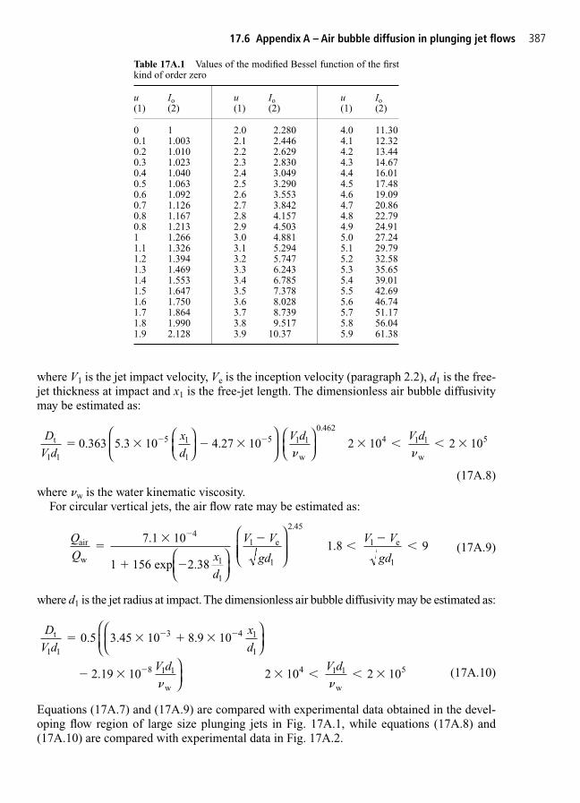
where V1 is the jet impact velocity, Ve is the inception velocity (paragraph 2.2), d1 is the free-jet thickness at impact and x1 is the free-jet length. The dimensionless air bubble diffusivitymay be estimated as:

(17A.8)where �w is the water kinematic viscosity.

For circular vertical jets, the air flow rate may be estimated as:

(17A.9)

where d1 is the jet radius at impact. The dimensionless air bubble diffusivity may be estimated as:

(17A.10)

Equations (17A.7) and (17A.9) are compared with experimental data obtained in the devel-oping flow region of large size plunging jets in Fig. 17A.1, while equations (17A.8) and(17A.10) are compared with experimental data in Fig. 17A.2.

DV d

xd

V d V d

t

1 1

3 4 1

1

8 1 1

w

4 1 1

w

5

0.5 3.45 10 8.9 10

2.19 10 2 10 2 10

� � �

� � � � � �

� �

�

� �

QQ x

d

V V

gd

V V

gdair

w 1

1

e

1

1 e

1

7.1 10

1 156 exp 2.38

9��

�

��

��

�41

2 45

1 8

.

.

DV d

xd

V d V dt

1 1

5 1

1

5 1 1

w

4 1 1

w

5 0.363 5.3 10 4.27 10 2 10 2 10� � � � � � � �� �

� �

0 462.

Table 17A.1 Values of the modified Bessel function of the firstkind of order zero

u Io u Io u Io(1) (2) (1) (2) (1) (2)

0 1 2.0 2.280 4.0 11.300.1 1.003 2.1 2.446 4.1 12.320.2 1.010 2.2 2.629 4.2 13.440.3 1.023 2.3 2.830 4.3 14.670.4 1.040 2.4 3.049 4.4 16.010.5 1.063 2.5 3.290 4.5 17.480.6 1.092 2.6 3.553 4.6 19.090.7 1.126 2.7 3.842 4.7 20.860.8 1.167 2.8 4.157 4.8 22.790.8 1.213 2.9 4.503 4.9 24.911 1.266 3.0 4.881 5.0 27.241.1 1.326 3.1 5.294 5.1 29.791.2 1.394 3.2 5.747 5.2 32.581.3 1.469 3.3 6.243 5.3 35.651.4 1.553 3.4 6.785 5.4 39.011.5 1.647 3.5 7.378 5.5 42.691.6 1.750 3.6 8.028 5.6 46.741.7 1.864 3.7 8.739 5.7 51.171.8 1.990 3.8 9.517 5.8 56.041.9 2.128 3.9 10.37 5.9 61.38

17.6 Appendix A – Air bubble diffusion in plunging jet flows 387

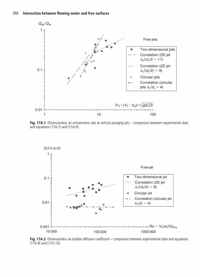
388 Interaction between flowing water and free surfaces

0.01

0.1

1

1 10 100

Two-dimensional jets

Correlation (2D jetx1/(d1/2 � 11)

Correlation (2D jetx1/(d1/2) � 9)

Circular jets

Correlation (circularjets x1/d1 � 4)

Free jets

Qair/Qw

Fr1�(V1�Ve)/ (gd1)/2

Fig. 17A.1 Dimensionless air entrainment rate at vertical plunging jets – comparison between experimental dataand equations (17A.7) and (17A.9).

10 000 100 000 1000 000

Two-dimensional jet

Correlation (2D jetx1/(d1/2) � 9)

Circular jet

Correlation (circular jetx1/d1 � 4)

0.001

0.01

0.1

1

Dt /(V1d1/2)

Re � V1(d1/2)/mw

Free-jet

Fig. 17A.2 Dimensionless air bubble diffusion coefficient – comparison between experimental data and equations(17A.8) and (17A.10).

17.7 Appendix B – Air bubble diffusion in self-aerated supercritical flows

In supercritical open channel flows, free-surface aeration is often observed. The phenome-non, called ‘white waters’, occurs when turbulence acting next to the free surface is largeenough to overcome both surface tension for the entrainment of air bubbles and buoyancy tocarry downwards the bubbles. Assuming a homogeneous air–water mixture for C � 90%, theadvective diffusion of air bubbles may be analytically predicted. At uniform equilibrium, theair concentration distribution is a constant with respect to the distance x in the flow direction.The continuity equation for air in the air–water flow yields:

(17B.1)

where C is the void fraction, Dt is the air bubble turbulent diffusivity, ur is the bubble risevelocity, � is the channel slope and y is measured perpendicular to the mean flow direction.The bubble rise velocity in a fluid of density �w(1 � C) equals:

(17B.2)

where (ur)Hyd is the rise velocity in hydrostatic pressure gradient (Chanson 1995a, 1997a). Afirst integration of the continuity equation for air in the equilibrium flow region leads to:

(17B.3)

where y� � y/Y90, D� � Dt/((ur)Hyd cos �Y90) is a dimensionless turbulent diffusivity and Y90is the location where C � 0.90. D� is the ratio of the air bubble diffusion coefficient to the

∂∂Cy D

C C�

��

� 1

1

u u Cr2 [( ) ] (1 )r Hyd

2� �

∂∂

∂∂

∂∂y

DCy y

u Ct r cos� � ( )

Notes1. Equation (17A.7) was first proposed by Brattberg and Chanson (1998) who measured

both void fraction and velocity distributions below impingement. The entrained airflow rate was estimated as:

where C and V were measured void fraction and air–water velocity respectively. Theresults were obtained for 4 � x1/d1 � 16.

2. Equation (17A.8) was deduced from the experiments of Chanson (1995a),Cummings (1996) and Brattberg and Chanson (1998) for 0.2 � x1/d1 � 9.

3. Equations (17A.9) and (17A.10) compared favourably with experimental dataobtained in fresh water, salt water and sea water for 0.2 � x1/d1 � 9 (Chanson et al.2002a, Chanson and Manasseh 2003).

4. It must be stressed that equations (17A.7)–(17A.10) are crude correlations. In prac-tice, D# and Qair/Qw must be deduced from measured distributions of void fractiondistributions (paragraph 17.5.1.2).

q CV yair d���

�

∫

17.7 Appendix B – Air bubble diffusion in self-aerated supercritical flows 389

390 Interaction between flowing water and free surfaces

rise velocity component normal to the flow direction times the characteristic transversedimension of the shear flow.

Assuming a homogeneous turbulence across the flow (i.e. D� constant), the integration ofequation (17B.3) yields:

(17B.4)

where tanh is the hyperbolic tangent function and K� a dimensionless integration constant.A relationship between D� and K� is deduced for C � 0.9 for y� � 1:

(17B.5)

where K* � tanh�1(��0.1�) � 0.327 450 15… The diffusivity and the mean air content Cmeandefined in terms of Y90 are related by:

(17B.6)

Advanced void fraction distribution models may be developed assuming a non-constant bub-ble diffusivity. Assuming that the diffusivity distribution satisfies:

the integration of equation (17B.1) yields:

(17B.7)C Ky

Y 1 exp

90

� � � ��

DC C

K C� �

�

� �

1 ( )�

C D KD

Kmean* * 2 tanh

2 tanh( )� �

��

1

K KD

� � �

1

2*

C KyD

1 tanh 2

2� � � ��

�

Notes1. The dimensionless bubble diffusion coefficient D� and integration constant K� are

functions of the depth-averaged air content Cmean only. They may be estimated as:

Cmean � 0.7

2. The depth-averaged air concentration is commonly defined in term of the character-istic air–water depth Y90:

CY

C yY

mean90

1

d�0

90

∫

KD

� � �

0.32745015 1

2

DC

C C� �

�

�

0.848 0.00302

1.1375 2.2925mean

mean mean21

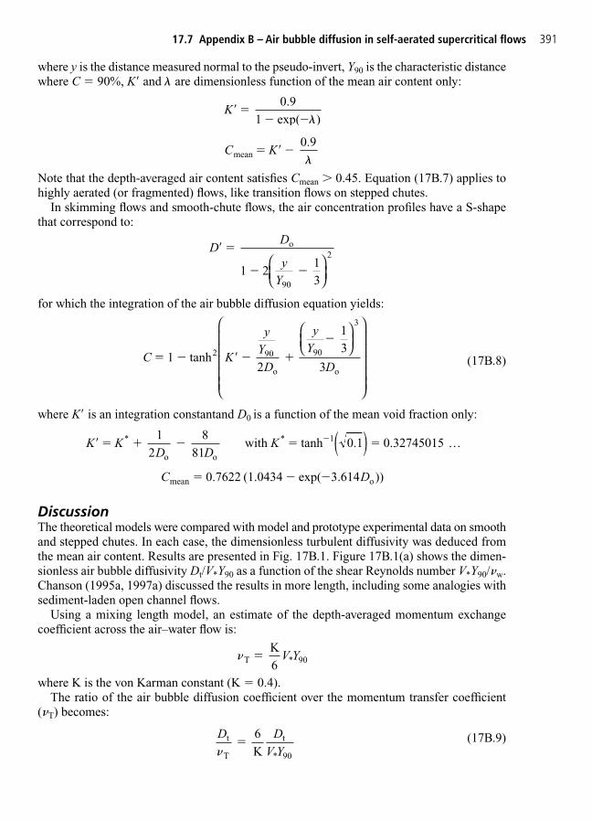
where y is the distance measured normal to the pseudo-invert, Y90 is the characteristic distancewhere C � 90%, K� and � are dimensionless function of the mean air content only:

Note that the depth-averaged air content satisfies Cmean � 0.45. Equation (17B.7) applies tohighly aerated (or fragmented) flows, like transition flows on stepped chutes.

In skimming flows and smooth-chute flows, the air concentration profiles have a S-shapethat correspond to:

for which the integration of the air bubble diffusion equation yields:

(17B.8)

where K� is an integration constantand D0 is a function of the mean void fraction only:

DiscussionThe theoretical models were compared with model and prototype experimental data on smoothand stepped chutes. In each case, the dimensionless turbulent diffusivity was deduced fromthe mean air content. Results are presented in Fig. 17B.1. Figure 17B.1(a) shows the dimen-sionless air bubble diffusivity Dt/V*Y90 as a function of the shear Reynolds number V*Y90/�w.Chanson (1995a, 1997a) discussed the results in more length, including some analogies withsediment-laden open channel flows.

Using a mixing length model, an estimate of the depth-averaged momentum exchangecoefficient across the air–water flow is:

where K is the von Karman constant (K � 0.4).The ratio of the air bubble diffusion coefficient over the momentum transfer coefficient

(�T) becomes:

(17B.9)D DV Y

t

T

t

* 90

6K�

�

�T * 90 K6

� V Y

C Dmean o 0.7622 (1.0434 exp( 3.614 ))� � �

K KD D

K� � � � �� 1

2

881

with tanh 0.32745015 *

o o

* 1 0 1.( ) K

C K

yYD

yY

D 1 tanh

2

132

o o

� � � �

�90 90

3

3

DD

yY

� �

� �

1 2 13

o

90

2

C Kmean 0.9

� � ��

K� �� �

0.9

1 exp( )�

17.7 Appendix B – Air bubble diffusion in self-aerated supercritical flows 391

392 Interaction between flowing water and free surfaces

Figure 17B.1(b) presents experimental results. In smooth chutes, the results show that self-aerated flows tend to exhibit large values of diffusion coefficients implying usually Dt/�T � 1while Dt/�T � 1 is usually observed in skimming flow down stepped chutes. The ratio Dt/�Tdescribes the combined effects of (1) the difference in the diffusion of a discrete particle (e.g.air bubble, sediment) and the diffusion of a small coherent fluid structure and (2) the influence

0.01(a)

0.1

1

1000 10 000 100 000 1000 000

Laboratory smooth chute

Prototype smooth chute

Stepped spillway

Dt /((V* )Y90)

(V*)Y90/m

0.01(b)

0.1

1

10

1000 10 000 100 000 1000 000

Laboratory smooth chutePrototype smooth chuteLaboratory stepped chute

Dt /nT

(V*)Y90/m

Fig. 17B.1 Dimensionless air bubble diffusion coefficient in self-aerated open channel flows. (a) Dimensionless airbubble diffusivity Dt/V*Y90 as a function of the shear Reynolds number V*Y90/�w. (b) Ratio of air bubble diffusivityto momentum exchange coefficient Dt/�T as a function of the shear Reynolds number V*Y90/�w.

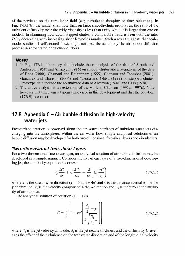
of the particles on the turbulence field (e.g. turbulence damping or drag reduction). In Fig. 17B.1(b), the reader shall note that, on large smooth-chute prototypes, the ratio of theturbulent diffusivity over the eddy viscosity is less than unity while it is larger than one onmodels. In skimming flow down stepped chutes, a comparable trend is seen with the ratioDt/�T decreasing with increasing shear Reynolds number. Such a result suggests that scale-model studies of self-aerated flows might not describe accurately the air bubble diffusionprocess in self-aerated open channel flows.

17.8 Appendix C – Air bubble diffusion in high-velocity water jets

Free-surface aeration is observed along the air–water interfaces of turbulent water jets dis-charging into the atmosphere. Within the air–water flow, simple analytical solutions of air bubble diffusion may be developed for both two-dimensional free-shear layers and circular jets.

Two-dimensional free-shear layersFor a two-dimensional free-shear layer, an analytical solution of air bubble diffusion may bedeveloped in a simple manner. Consider the free-shear layer of a two-dimensional develop-ing jet, the continuity equation becomes:

(17C.1)

where x is the streamwise direction (x � 0 at nozzle) and y is the distance normal to the thejet centreline, Vx is the velocity component in the x-direction and Dt is the turbulent diffusiv-ity of air bubbles.

The analytical solution of equation (17C.1) is:

(17C.2)

where V1 is the jet velocity at nozzle, d1 is the jet nozzle thickness and the diffusivity Dt aver-ages the effect of the turbulence on the transverse dispersion and of the longitudinal velocity

C

dy

DV

x

12

1 erf

2 t

� ��1

1

2

VCx

CVx y

DCyx

x∂∂

∂∂

∂∂

∂∂

t �

Notes1. In Fig. 17B.1, laboratory data include the re-analysis of the data of Straub and

Anderson (1958) and Aivazyan (1986) on smooth chutes and a re-analysis of the dataof Boes (2000), Chamani and Rajaratnam (1999), Chanson and Toombes (2001),Gonzalez and Chanson (2004) and Yasuda and Ohtsu (1999) on stepped chutes.Prototype data include the re-analysed data of Aivazyan (1986) and Cain (1978).

2. The above analysis is an extension of the work of Chanson (1995a, 1997a). Notehowever that there was a typographic error in this development and that the equation(17B.9) is correct.

17.8 Appendix C – Air bubble diffusion in high-velocity water jets 393

394 Interaction between flowing water and free surfaces

gradient. Dt is further assumed independent of the transverse direction y. The Gaussian errorfunction is defined as:

Circular jetsFor a circular water jet discharging into the atmosphere, the continuity equation for air becomes:

(17C.3)

where x is the longitudinal direction, r is the radial direction, Vx is the velocity componentin the x-direction and Dt is the turbulent diffusivity.

If the diffusivity term Dt averages the effects of the turbulent diffusion and the longitudi-nal velocity gradient, the solution of equation (17C.3) is a series of Bessel functions:

(17C.4)

where r90 is the radial distance where C � 0.9, Jo is the Bessel function of the first kind oforder zero, �n is the positive root of: Jo(r90�n) � 0 (Table 17C.1) and J1 is the Bessel functionof the first kind of order one.

Cr

J rJ r

DV

xn

n nn

n

0.9 1.8

exp90

o

1 90

t

11

� � �

�

( )( )

�

� ��2

∞

∑

VD

Cx

CD

Vx r r

rCr

x x

t t

1∂

∂∂∂

∂∂

∂∂

�

erf( ) 2

du t tu

� ��

exp( )2

0∫

Table 17C.1 Approximate solution of the roots of the equationJo(u) � 0 and J1(u) � 0

Root Jo(ui) � 0 J1(ui) � 0(1) (2) (3)

u1 2.4048 3.8317u2 5.5201 7.0156u3 8.6537 10.1735u4 11.7915 13.3237u5 14.0309 16.4706u6 18.0711 19.6159u7 18.0711 3.14159 19.6159 3.14159un1 un � un �

Reference: Spigel (1974).

Remarks1. The Bessel function of the first kind of order zero is defined as:

2. The Bessel function of the first kind of order one is:

J uu u u u

1

3 5

2

7

2 2 2

2

4

4 6

2 4 6 8 ( ) � �

�

� ��

� � �

2 22 2L

J uu u u

o

2 4

2

6

2 2 1

4

4 6 ( ) � �

��

� �

2 2 22 2 2L

DiscussionTheoretical results were compared with experimental data. The dimensionless air bubblediffusivity may be estimated as:

Two-dimensional (17C.5)

Circular jets (17C.6)

where d1 is the jet thickness and diameter at nozzle for two-dimensional and circularjets respectively. Experimental results are compared with equations (17C.5) and (17C.6) inFig. 17C.1.

DV d

V

gdt

1 1

8 1

1

5 10� � �

2 2.

DV d

V

gdt

1 1

4 1

1

3.6 10� � �

0 93.

0.00001

0.0001

0.001

0.01

0.1

1 10 100 1000

2D jetsCircular jetsCorrelation (2D jet)Correlation (circular jet)

V1/

D t /(V1d1)

gd1

Fig. 17C.1 Dimensionless air bubble diffusion coefficient in high-velocity water jets discharging into air – comparison with equation (17C.5) and (17C.6).

3. Chanson (1997a) integrated numerically equation (17C.4) for several values of thedimensionless diffusivity D� defined as:

4. Equation (17C.4) is valid close to and away from the deflector edge. It is a three-dimensional solution of the diffusion equation. It is valid also when the clear-watercore of the jet disappears and the jet becomes fully aerated.

′′DD x

V r t

o

�902

17.8 Appendix C – Air bubble diffusion in high-velocity water jets 395

396 Interaction between flowing water and free surfaces

17.9 Exercises

1. Considering a chute spillway ending with a flip bucket, describe the basic types of airentrainment upstream of the flip bucket, downstream of the ski jump, and in the down-stream plunge pool.

2. A vertical circular jet discharge into a plunge pool. The nozzle is located 0.1 m above the pool free surface and its diameter is 30 mm. Calculate the onset of air entrainment in terms of impact velocity V1 and nozzle flow rate Qw. Assume the fluid to be tap waterat 20°C.

3. A two-dimensional water jet plunges into a deep pool. The jet thickness and velocity at impact are respectively 28 mm and 6.5 m/s. Calculate and plot the void fraction distribution at 100 and 200 mm beneath the free surface. Assume the fluid to be tap waterat 20°C. Estimate the air entrainment rate and bubble diffusivity using Appendix A(Section 17.6).

4. At a vertical circular plunging jet, the water discharge is 0.011 m3/s and the nozzle veloc-ity is 8 m/s. For a free-jet length of 150 mm, the measured air entrainment rate at the plungepoint is 0.0032 m3/s. Calculate and plot the void fraction distribution at 150 and 250 mmbeneath the free surface. Assume the fluid to be tap water at 20°C. Estimate the bubblediffusivity using Appendix A (Section 17.6).

5. Predict the onset conditions for air entrainment down a 60° chute for 1, 10 and 50 mmbubbles. Assume the fluid to be tap water at 20°C.

6. Calculate the rise velocity of a 5 mm bubble in sea water at 20°C.7. In a smooth spillway chute, the depth-averaged void fraction and characteristic

depth Y90 are 0.31 and 0.95 m respectively. Calculate and plot the void fraction distribution.

8. An overflow spillway is to be designed with an uncontrolled crest followed by a steppedchute and a hydraulic jump dissipator. The maximum spillway capacity will be 4300 m3/s,and the flow velocity and depth at the end of the chute are expected to be 14 m/s and 2.9 m.(a) Calculate the prototype Froude, Reynolds and Weber number.

A 17:1 scale model of the spillway is to be built. (a) Based upon a Froude similitude,calculate the corresponding model Reynolds and Weber numbers.

9. What are the basic differences between optical fibre and resistivity probes?10. The data processing of a dual-tip probe gives the following auto-correlation and cross-

correlation functions. For a 8.1 mm spacing between probe sensors, calculate the localvelocity, dimensionless integral length scale and turbulence intensity.

Notes1. Equation (17C.5) was deduced from experiments conducted with 6 � Fr1 � 24 and

4 � V1 � 12 m/s (Brattberg et al. 1998).2. Equation (17C.6) derived from the re-analysis of experiments with 20 � Fr1 � 162

and 11 � V1 � 60 m/s.3. It must be stressed that equations (17C.5) and (17C.6) are crude correlations.

In practice, Dt must be deduced from measured distributions of void fraction distributions.

t (s) Rxx Rxy

0 1 0.0876370.00005 0.96586 0.0886160.0001 0.904278 0.0900610.00015 0.837674 0.0916510.0002 0.772436 0.0932760.00025 0.711249 0.0952480.0003 0.655413 0.097510.00035 0.605642 0.0999220.0004 0.562258 0.1027420.00045 0.524616 0.1057340.0005 0.491912 0.1087860.00055 0.463086 0.1118690.0006 0.437589 0.1150120.00065 0.415059 0.1184890.0007 0.395063 0.1219750.00075 0.377694 0.1256620.0008 0.362256 0.1300040.00085 0.348675 0.134370.0009 0.336638 0.139150.00095 0.32585 0.1442070.001 0.316006 0.1495150.00105 0.307062 0.155090.0011 0.298849 0.1609460.00115 0.291762 0.1669540.0012 0.286022 0.1724540.00125 0.281381 0.1770210.0013 0.276504 0.1806880.00135 0.271244 0.1837730.0014 0.266031 0.1859480.00145 0.261056 0.187340.0015 0.256012 0.1873260.00155 0.250623 0.1864350.0016 0.245439 0.185410.00165 0.240399 0.1845530.0017 0.235888 0.1843710.00175 0.231475 0.1853410.0018 0.227046 0.1874630.00185 0.22271 0.1900210.0019 0.218401 0.1934840.00195 0.214449 0.1981040.002 0.210557 0.2034440.00205 0.206111 0.2094270.0021 0.201267 0.2164440.00215 0.195988 0.2244430.0022 0.190544 0.2331220.00225 0.185114 0.2416780.0023 0.179563 0.2502380.00235 0.174289 0.2584370.0024 0.169248 0.2668990.00245 0.164254 0.2747920.0025 0.15909 0.2821630.00255 0.153975 0.2889340.0026 0.148747 0.2954280.00265 0.143654 0.3023440.0027 0.138966 0.3095730.00275 0.13483 0.3156760.0028 0.131087 0.3201770.00285 0.127764 0.3233190.0029 0.124473 0.325432

t (s) Rxx Rxy

0.00295 0.121275 0.3267850.003 0.118072 0.3272710.00305 0.115306 0.3273580.0031 0.112391 0.3272580.00315 0.109255 0.3269180.0032 0.106087 0.3254910.00325 0.103387 0.3229090.0033 0.100965 0.3192890.00335 0.098579 0.3150160.0034 0.096554 0.309430.00345 0.094845 0.3036740.0035 0.093291 0.2977040.00355 0.091654 0.2914960.0036 0.08964 0.2853050.00365 0.087022 0.2788540.0037 0.084282 0.2726680.00375 0.081846 0.2666080.0038 0.07964 0.2602370.00385 0.077468 0.2538140.0039 0.075573 0.2474290.00395 0.073941 0.241490.004 0.072307 0.2358190.00405 0.070747 0.2300180.0041 0.069671 0.223920.00415 0.068971 0.2179470.0042 0.068495 0.2121390.00425 0.068287 0.2068750.0043 0.06799 0.2019120.00435 0.067501 0.1974660.00445 0.066085 0.1899980.0045 0.065064 0.1857160.00455 0.063727 0.1811570.0046 0.062505 0.1768890.00465 0.061469 0.1728180.0047 0.060153 0.1687290.00475 0.058641 0.1646030.0048 0.057051 0.1602420.00485 0.055339 0.1562550.0049 0.053853 0.1530330.00495 0.052914 0.1502850.005 0.052618 0.1482780.00505 0.052643 0.1467520.0051 0.052923 0.1454610.00515 0.053662 0.1443030.0052 0.055273 0.1431390.00525 0.057347 0.1420090.0053 0.059371 0.1409950.00535 0.061346 0.1394220.0054 0.063119 0.13770.00545 0.064326 0.1354060.0055 0.064833 0.133160.00555 0.064109 0.130720.0056 0.062619 0.1280920.00565 0.060692 0.1255130.0057 0.058455 0.1234910.00575 0.056274 0.1220020.0058 0.054468 0.1206260.00585 0.053067 0.1191410.0059 0.052011 0.117174

t (s) Rxx Rxy

0.00595 0.050955 0.1149780.006 0.049636 0.1124990.00605 0.048382 0.1093450.0061 0.047107 0.1050750.00615 0.045534 0.0998680.0062 0.043833 0.0946090.00625 0.04223 0.0898960.0063 0.040903 0.0858580.00635 0.039846 0.0830350.0064 0.039394 0.0816680.00645 0.039291 0.0812870.0065 0.039019 0.0813110.00655 0.038766 0.0812080.0066 0.038915 0.0814690.00665 0.039606 0.0822320.0067 0.040581 0.0831080.00675 0.041433 0.0840160.0068 0.042165 0.085140.00685 0.042818 0.0863220.0069 0.043392 0.0872310.00695 0.044006 0.087550.007 0.044416 0.0876210.00705 0.044313 0.0874750.0071 0.043951 0.0870570.00715 0.043471 0.0863310.0072 0.042921 0.085590.00725 0.042795 0.0844270.0073 0.043508 0.0823520.00735 0.04455 0.0799250.0074 0.045083 0.0774060.00745 0.045225 0.0745220.0075 0.0712770.00755 0.0682650.0076 0.0652750.00765 0.062550.0077 0.0604970.00775 0.0591740.0078 0.0581940.00785 0.0573730.0079 0.0565510.00795 0.0556920.008 0.054520.00805 0.0532240.0081 0.0518310.00815 0.0506390.0082 0.0498570.00825 0.0494280.0083 0.0494240.00835 0.0499840.0084 0.0505050.00845 0.0509370.0085 0.0517810.00855 0.0532560.0086 0.0547810.00865 0.0562880.0087 0.0575420.00875 0.0581280.0088 0.058157

Answer: Tu � 0.46

17.9 Exercises 397

398 Interaction between flowing water and free surfaces

11. An overflow spillway is to be designed with an uncontrolled broad crest followed by astepped chute and a hydraulic jump dissipator. The width of the crest, chute and dissipa-tion basin will be 100 m. The crest level will be at 316.1 m R.L. and the design headabove crest level will be 3.1 m. The chute slope will be set at 51° and the step height willbe 0.5 m. The elevation of the chute toe will be set at 278.3 m R.L. The stepped chute willbe followed (without transition section) by a horizontal stilling basin.(a) Calculate the maximum discharge capacity of the spillway.(b) Compute the location of and flow properties at the inception point of free-surface

aeration.(c) Calculate the flow velocity and depth-averaged void fraction at the toe of the chute.(d) Calculate the residual power at the end of the chute (give the SI unit). Comment.Notes: In calculating the crest discharge capacity, assume that the discharge capacity of thebroad crest is 2% smaller than that of an ideal broad crest (for the same upstream headabove crest). In computing the velocity at the spillway toe, allow for energy losses by usingresults presented in the book. The residual power equals �gQwHres where Qw is the totalwater discharge and Hres is the residual total head at chute toe taking the chute toe elevationas datum. Assume the Darcy friction factor of non-aerated stepped chute to be 0.24.

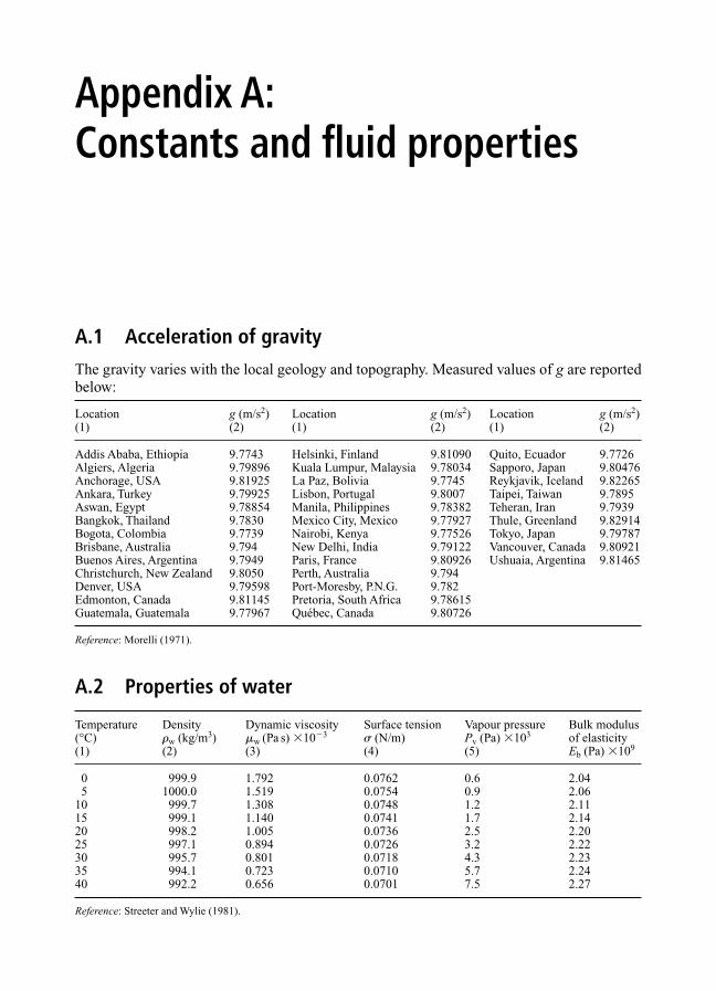
Appendix A:Constants and fluid properties

A.1 Acceleration of gravity

The gravity varies with the local geology and topography. Measured values of g are reportedbelow:

Location g (m/s2) Location g (m/s2) Location g (m/s2) (1) (2) (1) (2) (1) (2)

Addis Ababa, Ethiopia 9.7743 Helsinki, Finland 9.81090 Quito, Ecuador 9.7726Algiers, Algeria 9.79896 Kuala Lumpur, Malaysia 9.78034 Sapporo, Japan 9.80476Anchorage, USA 9.81925 La Paz, Bolivia 9.7745 Reykjavik, Iceland 9.82265Ankara, Turkey 9.79925 Lisbon, Portugal 9.8007 Taipei, Taiwan 9.7895Aswan, Egypt 9.78854 Manila, Philippines 9.78382 Teheran, Iran 9.7939Bangkok, Thailand 9.7830 Mexico City, Mexico 9.77927 Thule, Greenland 9.82914Bogota, Colombia 9.7739 Nairobi, Kenya 9.77526 Tokyo, Japan 9.79787Brisbane, Australia 9.794 New Delhi, India 9.79122 Vancouver, Canada 9.80921Buenos Aires, Argentina 9.7949 Paris, France 9.80926 Ushuaia, Argentina 9.81465Christchurch, New Zealand 9.8050 Perth, Australia 9.794Denver, USA 9.79598 Port-Moresby, P.N.G. 9.782Edmonton, Canada 9.81145 Pretoria, South Africa 9.78615Guatemala, Guatemala 9.77967 Québec, Canada 9.80726

Reference: Morelli (1971).

A.2 Properties of water

Temperature Density Dynamic viscosity Surface tension Vapour pressure Bulk modulus (°C) �w (kg/m3) �w (Pa s) �10�3 (N/m) Pv (Pa) �103 of elasticity (1) (2) (3) (4) (5) Eb (Pa) �109

0 999.9 1.792 0.0762 0.6 2.045 1000.0 1.519 0.0754 0.9 2.06

10 999.7 1.308 0.0748 1.2 2.1115 999.1 1.140 0.0741 1.7 2.1420 998.2 1.005 0.0736 2.5 2.2025 997.1 0.894 0.0726 3.2 2.2230 995.7 0.801 0.0718 4.3 2.2335 994.1 0.723 0.0710 5.7 2.2440 992.2 0.656 0.0701 7.5 2.27

Reference: Streeter and Wylie (1981).

A.3 Gas properties

Basic equations

The state equation of perfect gas is:

(A.1)

where P is the absolute pressure (in Pascal), � is the gas density (in kg/m3), T is the absolutetemperature (in Kelvin) and R is the gas constant (in J/kg K) (see table below).

For a perfect gas, the specific heat at constant pressure Cp and the specific heat at constantvolume Cv are related to the gas constant as:

(A.2a)

(A.2b)

where � is the specific heat ratio (i.e. � � Cp /Cv).During an isentropic transformation of perfect gas, the following relationships hold:

(A.3a)

(A.3b)

Physical properties

Gas Formula Gas constant Specific heat (J/kg K) Specific heat ratio R (J/kg K)

Cp Cv

�

(1) (2) (3) (4) (5) (6)

Perfect gas

Mono-atomic gas (e.g. He)

Di-atomic gas (e.g. O2)

Poly-atomic gas (e.g. CH4) 4R 3R

Real gasa

Air 287 1.004 0.716 1.40Helium He 2077.4 5.233 3.153 1.67Nitrogen N2 297 1.038 0.741 1.40Oxygen O2 260 0.917 0.657 1.40Water vapour H2O 462 1.863 1.403 1.33

aAt low pressures and at 299.83 K.Reference: Streeter and Wylie (1981).

43

75

52

R72

R

53

32

R52

R

T P constant)/(1�� � �

P

��� constant

C Cp v R�

Cp 1

R��

� �

P T R� �

400 Appendix A

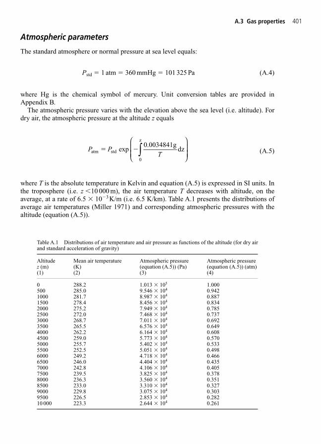
Atmospheric parameters

The standard atmosphere or normal pressure at sea level equals:

Pstd � 1 atm � 360 mmHg � 101 325 Pa (A.4)

where Hg is the chemical symbol of mercury. Unit conversion tables are provided inAppendix B.

The atmospheric pressure varies with the elevation above the sea level (i.e. altitude). Fordry air, the atmospheric pressure at the altitude z equals

(A.5)

where T is the absolute temperature in Kelvin and equation (A.5) is expressed in SI units. Inthe troposphere (i.e. z �10 000 m), the air temperature T decreases with altitude, on the average, at a rate of 6.5 � 10�3K/m (i.e. 6.5 K/km). Table A.1 presents the distributions ofaverage air temperatures (Miller 1971) and corresponding atmospheric pressures with thealtitude (equation (A.5)).

P PTatm std

0

z

exp0.0034841g

dz� �∫

A.3 Gas properties 401

Table A.1 Distributions of air temperature and air pressure as functions of the altitude (for dry airand standard acceleration of gravity)

Altitude Mean air temperature Atmospheric pressure Atmospheric pressure z (m) (K) (equation (A.5)) (Pa) (equation (A.5)) (atm) (1) (2) (3) (4)

0 288.2 1.013 � 105 1.000500 285.0 9.546 � 104 0.9421000 281.7 8.987 � 104 0.8871500 278.4 8.456 � 104 0.8342000 275.2 7.949 � 104 0.7852500 272.0 7.468 � 104 0.7373000 268.7 7.011 � 104 0.6923500 265.5 6.576 � 104 0.6494000 262.2 6.164 � 104 0.6084500 259.0 5.773 � 104 0.5705000 255.7 5.402 � 104 0.5335500 252.5 5.051 � 104 0.4986000 249.2 4.718 � 104 0.4666500 246.0 4.404 � 104 0.4357000 242.8 4.106 � 104 0.4057500 239.5 3.825 � 104 0.3788000 236.3 3.560 � 104 0.3518500 233.0 3.310 � 104 0.3279000 229.8 3.075 � 104 0.3039500 226.5 2.853 � 104 0.28210 000 223.3 2.644 � 104 0.261

Viscosity of air

Viscosity and density of air at 1.0 atm:

Temperature (K) �air (Pa s) �10�6 �air (kg/m3) (1) (3) (3)

300 18.4 1.177400 22.7 0.883500 26.7 0.705600 29.9 0.588

The viscosity of air at standard atmosphere is commonly fitted by the Sutherland formula(Sutherland 1883):

(A.6)

A simpler correlation is:

(A.7)

where �air is in Pa s, and the temperature T and reference temperature To are expressed inKelvin.

�

�air

air o o

( )( )

TT

TT

�

0 76.

�air 17.16 10 6 273.1

110.6

� � �

TT

3 2

383 7/

.

402 Appendix A

Appendix B:Unit conversions

B.1 Introduction

The systems of units derived from the metric system have gradually been replaced a singlesystem, called the Système International d’Unités (SI unit system, or International System ofUnits). The basic SI units are the metre, kilogramme, second, Ampere, Kelvin, mole and can-dela. Supplementary units are the radian and the steradian. All other SI units derive from thebasic units. Conversion tables are provided in this appendix. Basic references in unit conver-sions include Degremont (1979) and ISO (1979).

Unit symbols are written in small letters (i.e. m for metre, kg for kilogramme) but a capi-tal is used for the first letter when the name of the unit derives from a surname (e.g. Pa afterBlaise Pascal, N after Isaac Newton). Multiples and submultiples of SI units are formed byadding one prefix to the name of the unit: e.g. km for kilometre, cm for centimetre, dam fordecametre, �m for micrometre (or micron).

Multiple/submultiple factor Prefix Symbol

1 �109 giga G1 �106 mega M1 �103 kilo k1 �102 hecto d1 �101 deca da

1 �10�1 deci d1 �10�2 centi c1 �10�3 milli m1 � 10�6 micro �1 � 10�9 nano n

B.2 Units and conversion factors

Quantity Unit (symbol) Conversion Comments (1) (2) (3) (4)

Length 1 inch (in) � 25.4 � 10�3 m Exactly1 foot (ft) � 0.3048 m Exactly1 yard (yd) � 0.9144 m Exactly1 mil � 25.4 � 10�6m 1/1000 inch1 mile � 1.609 344 m Exactly

Area 1 square inch (in2) � 6.4516 � 10�4m2 Exactly1 square foot (ft2) � 0.092 903 06 m2 Exactly

Volume 1 litre (L) � 1.0 � 10�3m3 Exactly. Previous symbol: l

1 cubic inch (in3) � 16.387 064 � 10�6m3 Exactly1 cubic foot (ft3) � 28.316 8 � 10�3m3 Exactly1 gallon UK (gal UK) � 4.546 09 � 10�3m3

1 gallon US (gal US) � 3.785 41 � 10�3m3

1 barrel US � 158.987 � 10�3m3 For petroleum, etc.

Velocity 1 foot per second (ft/s) � 0.3048 m/s Exactly1 mile per hour (mph) � 0.447 04 m/s Exactly

Acceleration 1 foot per second squared (ft/s2) � 0.3048 m/s2 Exactly

Mass 1 pound (lb or lbm) � 0.453 592 37 kg Exactly1 ton UK � 1016.05 kg1 ton US � 907.185 kg

Density 1 pound per cubic foot (lb/ft3) � 16.0185 kg/m3

Force 1 kilogram-force (kgf) � 9.806 65 N (exactly) Exactly1 pound force (lbf) � 4.448 221 615 2605 N

Moment of force 1 foot pound force (ft lbf) � 1.355 82 N m

Pressure 1 Pascal (Pa) � 1 N/m2

1 standard atmosphere (atm) � 101 325 Pa � 760 mm of mercury at Exactly

normal pressure (i.e. mmHg)

1 bar � 105Pa Exactly1 Torr � 133.322 Pa1 conventional metre of � 9.806 65 � 103Pa Exactlywater (m of H2O)1 conventional meter of � 1.333 224 � 105Pamercury (m of Hg)1 Pound per Square Inch (PSI) � 6.894 757 2 � 103Pa

Temperature T (Celsius) � T (Kelvin) � 273.16 0 Celsius is 0.01 K below the temperature of the triple point of water.

T (Fahrenheit) � T (Celcius) 95 32

T (Rankine) �95 T (Kelvin)

Dynamic viscosity 1 Pa s � 0.006 720 lbm/ft/s1 Pa s � 10 Poises Exactly1 N s/m2 � 1 Pa s Exactly1 Poise (P) � 0.1 Pa s Exactly1 milliPoise (mP) � 1.0 � 10�4Pa s Exactly

Kinematic viscosity 1 square foot per second (ft2/s) � 0.092 903 0 m2/s1 m2/s � 10.7639 ft2/s1 m2/s � 104 Stokes

Surface tension 1 dyne/cm � 0.99987 � 10�3N/m1 dyne/cm � 5.709 � 10�6 pound/inch

(Contd)

404 Appendix B

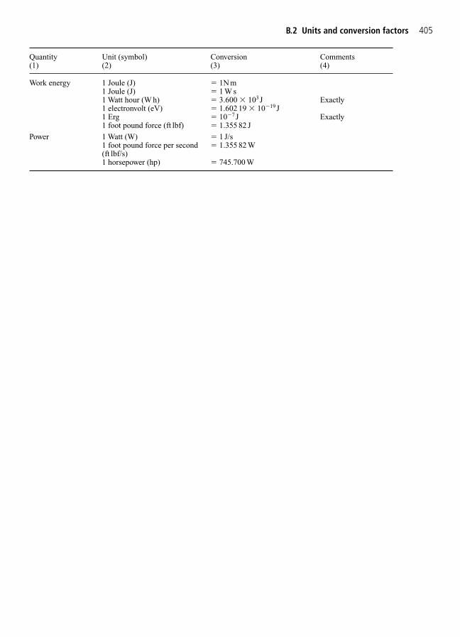
Quantity Unit (symbol) Conversion Comments (1) (2) (3) (4)

Work energy 1 Joule (J) � 1N m1 Joule (J) � 1 W s1 Watt hour (W h) � 3.600 � 103J Exactly1 electronvolt (eV) � 1.602 19 � 10�19J1 Erg � 10�7J Exactly1 foot pound force (ft lbf) � 1.355 82 J

Power 1 Watt (W) � 1 J/s1 foot pound force per second � 1.355 82 W(ft lbf/s)1 horsepower (hp) � 745.700 W

B.2 Units and conversion factors 405

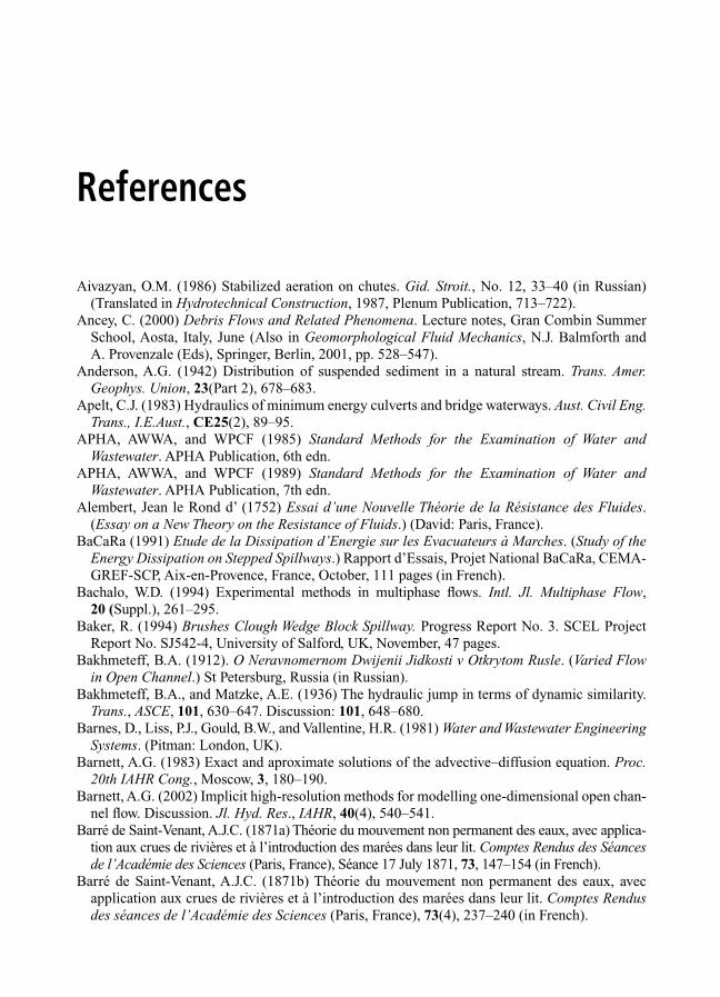
References

Aivazyan, O.M. (1986) Stabilized aeration on chutes. Gid. Stroit., No. 12, 33–40 (in Russian)(Translated in Hydrotechnical Construction, 1987, Plenum Publication, 713–722).

Ancey, C. (2000) Debris Flows and Related Phenomena. Lecture notes, Gran Combin SummerSchool, Aosta, Italy, June (Also in Geomorphological Fluid Mechanics, N.J. Balmforth and A. Provenzale (Eds), Springer, Berlin, 2001, pp. 528–547).

Anderson, A.G. (1942) Distribution of suspended sediment in a natural stream. Trans. Amer.Geophys. Union, 23(Part 2), 678–683.

Apelt, C.J. (1983) Hydraulics of minimum energy culverts and bridge waterways. Aust. Civil Eng.Trans., I.E.Aust., CE25(2), 89–95.

APHA, AWWA, and WPCF (1985) Standard Methods for the Examination of Water andWastewater. APHA Publication, 6th edn.

APHA, AWWA, and WPCF (1989) Standard Methods for the Examination of Water andWastewater. APHA Publication, 7th edn.

Alembert, Jean le Rond d’ (1752) Essai d’une Nouvelle Théorie de la Résistance des Fluides.(Essay on a New Theory on the Resistance of Fluids.) (David: Paris, France).

BaCaRa (1991) Etude de la Dissipation d’Energie sur les Evacuateurs à Marches. (Study of theEnergy Dissipation on Stepped Spillways.) Rapport d’Essais, Projet National BaCaRa, CEMA-GREF-SCP, Aix-en-Provence, France, October, 111 pages (in French).

Bachalo, W.D. (1994) Experimental methods in multiphase flows. Intl. Jl. Multiphase Flow, 20 (Suppl.), 261–295.

Baker, R. (1994) Brushes Clough Wedge Block Spillway. Progress Report No. 3. SCEL ProjectReport No. SJ542-4, University of Salford, UK, November, 47 pages.

Bakhmeteff, B.A. (1912). O Neravnomernom Dwijenii Jidkosti v Otkrytom Rusle. (Varied Flowin Open Channel.) St Petersburg, Russia (in Russian).

Bakhmeteff, B.A., and Matzke, A.E. (1936) The hydraulic jump in terms of dynamic similarity.Trans., ASCE, 101, 630–647. Discussion: 101, 648–680.

Barnes, D., Liss, P.J., Gould, B.W., and Vallentine, H.R. (1981) Water and Wastewater EngineeringSystems. (Pitman: London, UK).

Barnett, A.G. (1983) Exact and aproximate solutions of the advective–diffusion equation. Proc.20th IAHR Cong., Moscow, 3, 180–190.

Barnett, A.G. (2002) Implicit high-resolution methods for modelling one-dimensional open chan-nel flow. Discussion. Jl. Hyd. Res., IAHR, 40(4), 540–541.

Barré de Saint-Venant, A.J.C. (1871a) Théorie du mouvement non permanent des eaux, avec applica-tion aux crues de rivières et à l’introduction des marées dans leur lit. Comptes Rendus des Séancesde l’Académie des Sciences (Paris, France), Séance 17 July 1871, 73, 147–154 (in French).

Barré de Saint-Venant, A.J.C. (1871b) Théorie du mouvement non permanent des eaux, avecapplication aux crues de rivières et à l’introduction des marées dans leur lit. Comptes Rendusdes séances de l’Académie des Sciences (Paris, France), 73(4), 237–240 (in French).

References 407

Bartsch-Winkler, S., Emmanuel, R.P., and Winkler, G.R. (1985) Reconnaissance hydrology and sus-pended sediment analysis, Turnagain Arm Estuary, Upper Cook Inlet. US Geolog. Surv. Circ.,967, 48–52.

Bazin, H. (1865a) Recherches expérimentales sur l’ecoulement de l’eau dans les canaux décou-verts. (Experimental research on water flow in open channels.) Mémoires Présentés par DiversSavants à l’Académie des Sciences (Paris, France), 19, 1–494 (in French).

Bazin, H. (1865b) Recherches expérimentales sur la propagation des ondes. (Experimental researchon wave propagation.) Mémoires Présentés par Divers Savants à l’Académie des Sciences(Paris, France), 19, 495–644 (in French).

Beer, T., and Young, P.C. (1983) Longitudinal dispersion in natural streams. Jl. Environ. Eng.,ASCE, 109(5), 1049–1067.

Bélanger, J.B. (1828) Essai sur la Solution Numérique de Quelques Problèmes Relatifs auMouvement Permanent des Eaux Courantes. (Essay on the Numerical Solution of SomeProblems Relative to Steady Flow of Water.) (Carilian-Goeury: Paris, France) (in French).

Benet, F., and Cunge, J.A. (1971) Analysis of experiments on secondary undulations caused bysurge waves in trapezoidal channels. Jl. Hyd. Res., IAHR, 9(1), 11–33.

Bhargava, D.S., and Ojha, C.S.P. (1990) Genesis of free hydraulic jumps for better mixing. Wat.Res., 24(8), 1003–1010.

Bin, A.K. (1993) Gas entrainment by plunging liquid jets. Chem. Eng. Sci., 48(21), 3585–3630.

Blanckaert, K., and Graf, W.H. (2001) Mean flow and turbulence in open-channel bend. Jl. Hyd.Eng., ASCE, 127(10) 835–847.

Blasius, H. (1913) Das ähnlichkeitsgesetz bei reibungsvorgängen in flüssigkeiten. Forschg. Arb.Ing.-Wes., 134 (Berlin, Germany) (in German).

Boes, R.M. (2000) Zweiphasenstroömung und Energieumsetzung an Grosskaskaden. (Two-PhaseFlow and Energy Dissipation on Cascades.) Ph.D. Thesis, VAW-ETH, Zürich, Switzerland (inGerman) (Also Mitt. der Versuchsanstalt fur Wasserbau, Hydrologie und Glaziologie, ETH-Zurich, Switzerland, No. 166).

Bornschein, A., and Pohl, R. (2003) Dam break during the flood in Saxon/Germay in August2002. Proc. 30th IAHR Biennial Cong., Thessaloniki, Greece, J. Ganoulis, and P. Prinos (Eds),C2, 229–236.

Bossut, Abbé C. (1772) Traité Elémentaire d’Hydrodynamique. (Elementary Treaty onHydrodynamics.) 1st edn (Paris, France) (in French) (2nd edn: 1786, Paris, France; 3rd edn:1796, Paris, France).

Boussinesq, J.V. (1877) Essai sur la théorie des eaux courantes. (Essay on the theory of waterflow.) Mémoires Présentés par Divers Savants à l’Académie des Sciences (Paris, France), 23,Series 3, No. 1, Suppl. 24, 1–680 (in French).

Boussinesq, J.V. (1896) Théorie de l’ecoulement tourbillonnant et tumultueux des liquides dansles lits rectilignes à grande section (tuyaux de conduite et canaux découverts) quand cet ecoule-ment s’est régularisé en un régime uniforme, c’est-à-dire, moyennement pareil à travers toutesles sections Normales du lit. (Theory of turbulent and tumultuous flow of liquids in prismaticchannels of large cross-sections (pipes and open channels) when the flow is uniform, i.e. con-stant in average at each cross-section along the flow direction.) Comptes Rendus des Séancesde l’Académie des Sciences (Paris, France), 122, 1290–1295 (in French).

Bowie, G., Mills, W.B., Fordella, D.B., Campbell, C.L., Pagenkopf, J.R., Rupp, G.L., Johnson, K.M.,Chan, P.W.H., Cherini, S., and Chamberlin, C.E. (1985) Rates, Constants, and KineticsFormulations in Surface Water Quality Modeling. Tetra Tech. Report, No. EPA/600/3-85-040,2nd edn, 475 pages.

Boxall, J.B., Guymer, I., and Marion, A. (2003) Transverse mixing in sinuous natural open chan-nel flows. Jl. Hyd. Res., IAHR, 41(3), 153–165.

408 References

Boys, P.F.D. du (1879) Etude du Régime et de l’Action exercée par les Eaux sur un Lit á Fond deGraviers indéfiniment affouillable. (Study of flow regime and force exerted on a gravel bed ofinfinite depth.) Ann. Ponts et Chaussées, Paris, France, série 5, 19, 141–195 (in French).

Brattberg, T., and Chanson, H. (1998) Air entrapment and air bubble dispersion at two-dimensionalplunging water jets. Chem. Eng. Sci., 53(24, December), 4113–4127. Errata: 1999, 54(12), 1925.

Brattberg, T., Chanson, H., and Toombes, L. (1998) Experimental investigations of free-surfaceaeration in the developing flow of two-dimensional water jets. Jl. Fluids Eng., Trans. ASME,120(4), 738–744.

Bresse, J.A. (1860) Cours de Mécanique Appliquée Professé à l’Ecole des Ponts et Chaussées.(Course in Applied Mechanics Lectured at the Pont-et-Chaussées Engineering School.)(Mallet-Bachelier: Paris, France) (in French).

Brodie, I. (1988) Breaching of Coastal Lagoons. A Model Study. Masters Thesis, M.Sc.,University of New South Wales, Australia.

Brown, G.O. (2002) Henry Darcy and the making of a law. Wat. Res. Res., 38(7), Paper 11, 11-1–11-12.Brown, P.P., and Lawler, D.F. (2003) Sphere drag and settling velocity revisited. Jl. Environ. Eng.,

ASCE, 129(3), 222–231.Buat, P.L.G. du (1779) Principes d’Hydraulique, vérifiés par un grand nombre d’expériences

faites par ordre du gouvernement. (Hydraulic Principles, verified by a large number of experi-ments.) 1st edn (Imprimerie de Monsieur: Paris, France) (in French) (2nd edn: 1786, Paris,France, 2 volumes; 3rd edn: 1816, Paris, France, 3 volumes).

Bushnell, D.M., and Hefner, J.N. (1990) Viscous drag reduction in boundary layers. AIAAPublication, Progress in Astronautics and Aeronautics, 123, Washington DC, USA, 517 pages.

Cain, P. (1978) Measurements within Self-Aerated Flow on a Large Spillway. Ph.D. Thesis, Ref.78-18, Department of Civil Engineering, University of Canterbury, Christchurch, New Zealand.

Cain, P., and Wood, I.R. (1981). Measurements of self-aerated flow on a spillway. Jl. Hyd. Div.,ASCE, 107(HY11), 1425–1444.

Capart, H., and Young, D.L. (1998) Formation of a jump by the dam-break wave over a granularbed. Jl. Fluid Mech., 372, 165–187.

Carslaw, H.S., and Jaeger, J.C. (1959) Conduction of Heat in Solids. (Oxford University Press:London, UK) 2nd edn, 510 pages.

Cartellier, A. (1992) Simultaneous void fraction measurement, bubble velocity, and size estimateusing a single optical probe in gas–liquid tow-phase flows. Rev. Sci. Instrum., 63(11), 5442–5453.

Chamani, M.R., and Rajaratnam, N. (1999) Characteristics of skimming flow over stepped spill-ways. Jl. Hyd. Eng., ASCE, 125(4), 361–368. Discussion: 126(11), 860–872. Closure: 126(11),872–873.

Chang, K.A., Lim, H.J., and Su, C.B. (2003) Fiber optic reflectometer for velocity and fractionratio measurements in multiphase flows. Rev. Scientif. Inst., 74(7), 3559–3565. Discussion: 75(in print).

Chanson, H. (1988) A Study of Air Entrainment and Aeration Devices on a Spillway Model. Ph.D.Thesis, Ref. 88-8, Department of Civil Engineering, University of Canterbury, New Zealand.

Chanson, H.(1989) Study of air entrainment and aeration devices. Jl. Hyd. Res., IAHR, 27(3), 301–319.Chanson, H. (1993) Self-aerated flows on chutes and spillways. Jl. Hyd. Eng., ASCE, 119(2),

220–243. Discussion: 120(6), 778–782.Chanson, H. (1994) Drag reduction in open channel flow by aeration and suspended load. Jl. Hyd.

Res., IAHR, 32(1), 87–101.Chanson, H. (1995a) Air Bubble Entrainment in Free-Surface Turbulent Flows. Experimental

Investigations. Report CH46/95, Department of Civil Engineering, University of Queensland,Australia, June, 368 pages.

Chanson, H. (1995b) Flow Characteristics of Undular Hydraulic Jumps. Comparison with Near-Critical Flows. Report CH45/95, Department of Civil Engineering, University of Queensland,Australia, June, 202 pages.

References 409

Chanson, H. (1997a) Air Bubble Entrainment in Free-Surface Turbulent Shear Flows. (AcademicPress: London, UK), 401 pages. {http://www.uq.edu.au/�e2hchans/reprints/book2.htm}.

Chanson, H. (1997b) Air bubble entrainment in open channels. Flow structure and bubble sizedistributions. Intl. Jl. Multiphase Flow, 23(1), 193–203.

Chanson, H. (1999a) The Hydraulics of Open Channel Flows: An Introduction. (Edward Arnold:London, UK) 1st edn, 512 pages (ISBN 0 340 74067 1). {http://www.uq.edu.au/�e2hchans/reprints/errata.htm}.

Chanson, H. (1999b) Turbulent open-channel flows: drop-generation and self-aeration.Discussion. Jl. Hyd. Eng., ASCE, 125(6), 668–670.

Chanson, H. (2000) Boundary shear stress measurements in undular flows: application to stand-ing wave bed forms. Wat. Res. Res., 36(10), 3063–3076.

Chanson, H. (2001a) Flow field in a tidal bore: a physical model. Proc. 29th IAHR Cong., Beijing,China, Theme E, Tsinghua University Press, Beijing, G. Li (Ed.), pp. 365–373. (CD-ROM,Tsinghua University Press).

Chanson, H. (2001b) The Hydraulics of Stepped Chutes and Spillways. (Balkema: Lisse, TheNetherlands), 418 pages. {http://www.uq.edu.au/�e2hchans/reprints/book4.htm}

Chanson, H. (2002a) Very strong free-surface aeration in turbulent flows: entrainment mecha-nisms and air–water flow structure at the pseudo free-surface. In Interaction of StrongTurbulence with Free Surfaces, World Scientific, Advances in Coastal and Ocean EngineeringSeries, 8, Singapore, M. Brocchini, and D.H. Peregrine (Eds), 8, 65–98 (ISBN 981-02-4952-7).

Chanson, H., (2002b) An Experimental Study of Roman Dropshaft Operation: Hydraulics, Two-Phase Flow, Acoustics. Report CH50/02, Department of Civil Engineering, University ofQueensland, Brisbane, Australia, 99 pages. {http://www.uq.edu.au/�e2hchans/reprints/ ch5002.zip}

Chanson, H. (2002c) Air–water flow measurements with intrusive phase-detection probes. Canwe improve their interpretation? Jl. Hyd. Eng., ASCE, 128(3), 252–255.

Chanson, H. (2003a) Mixing and dispersion in tidal bores. A review. Proc. Intl. Conf. onEstuaries and Coasts (ICEC-2003), Hangzhou, China, November.

Chanson, H. (2003b) Sudden Flood Release Down a Stepped Cascade. Unsteady Air–Water FlowMeasurements. Applications to Wave Run-Up, Flash Flood and Dam Break Wave. ReportCH51/03, Department of Civil Engineering, University of Queensland, Brisbane, Australia,142 pages. {http://www.uq.edu.au/�e2hchans/reprints/ch5103.zip}

Chanson, H. (2003c) Two-phase flow characteristics of an unsteady dam break wave flow. Proc. 30th IAHR Biennial Cong., Thessaloniki, Greece, J. Ganoulis, and P. Prinos (Eds), C2,237–244.

Chanson, H. (2003d) History of minimum energy loss weirs and culverts. 1960–2002. Proc. 30thIAHR Biennial Cong., Thessaloniki, Greece, J. Ganoulis, and P. Prinos (Eds), E, 379–387.

Chanson, H. (2004a) Drag reduction in skimming flow on stepped spillways by aeration. Jl. Hyd.Research, IAHR, 42 (in print).

Chanson, H. (2004b) The Hydraulics of Open Channel Flows: An Introduction. (Butterworth-Heinemann: Oxford, UK) 2nd edn (ISBN 0 7506 5978 5).

Chanson, H. (2004c) Enhancing students’ motivation in the undergraduate teaching of hydraulicengineering: the role of field works. Jl. Prof. Issues Eng. Educ. Pract., ASCE, 130 (in print).

Chanson, H. (2004d) Free-Surface Aeration in Dam Break Waves: An Experimental Study. Proc.Intl. Conf. on Hydraulics of Dams and River Structures, Tehran, Iran, Balkema Publisher.

Chanson, H., and Brattberg, T. (2000) Experimental study of the air-–water shear flow in ahydraulic jump. Intl. Jl. Multiphase Flow, 26(4), 583–607.

Chanson, H., and Cummings, P.D. (1992) Aeration of the Ocean due to Plunging Breaking Waves.Research Report No. CE142, Department of Civil Engineering, University of Queensland,Australia, November, 42 pages.

Chanson, H., and James, P. (1998) Teaching case studies in reservoir siltation and catchment ero-sion. Intl. Jl. Eng. Educ., 14(4), 265–275. {http://www.uq.edu.au/�e2hchans/res_silt.html}

410 References

Chanson, H., and Manasseh, R. (2003) Air entrainment processes in a circular plunging jet. Voidfraction and acoustic measurements. Jl. Fluids Eng., Trans. ASME, 125(5, September),910–921.

Chanson, H., and Qiao, G.L. (1994a) Air Bubble Entrainment and Gas Transfer at HydraulicJumps. Research Report No. CE149, Department of Civil Engineering, University of Queensland,Australia, August, 68 pages.

Chanson, H., and Qiao, G.L. (1994b) Drag reduction in hydraulics flows. Proc. Intl. Conf. onHydraulics in Civil Eng., I.E.Aust., Brisbane, Australia, 15–17 February, pp. 123–128.

Chanson, H., and Toombes, L. (2000) Stream reaeration in nonuniform flow: macroroughnessenhancement. Discussion. Jl. Hyd. Eng., ASCE, 126(3), 222–224.

Chanson, H., and Toombes, L. (2001) Experimental Investigations of Air Entrainment inTransition and Skimming Flows Down a Stepped Chute. Application to Embankment OverflowStepped Spillways. Research Report No. CE158, Department of Civil Engineering, Universityof Queensland, Brisbane, Australia, July, 74 pages.

Chanson, H., and Toombes, L. (2002) Air–water flows down stepped chutes: turbulence and flowstructure observations. Intl. Jl. Multiphase Flow, 27(11), 1737–1761.

Chanson, H., Aoki, S., and Maruyama, M. (2000) Experimental Investigations of Wave RunupDownstream of Nappe Impact. Applications to Flood Wave Resulting from Dam Overtoppingand Tsunami Wave Runup. Coastal/Ocean Engineering Report, No. COE00-2, Department ofArchitecture and Civil Engineering, Toyohashi University of Technology, Japan, 38 pages.

Chanson, H., Aoki, S., and Hoque, A. (2002a) Similitude of Air Bubble Entrainment andDispersion in Vertical Circular Plunging Jet Flows. An Experimental Study with Freshwater,Salty Freshwater and Seawater. Coastal/Ocean Engineering Report, No. COE02-1, Departmentof Architecture and Civil Engineering, Toyohashi University of Technology, Japan, 94 pages.{http://www.uq.edu.au/�e2hchans/reprints/tut02.zip}

Chanson, H., Yasuda, Y., and Ohtsu, I. (2002b) Flow resistance in skimming flows and its model-ling. Can. Jl. Civ. Eng., 29(6), 809–819.

Chanson, H., Aoki, S., and Hoque, A. (2002c) Scaling bubble entrainment and dispersion in vertical circular plunging jet flows: freshwater versus seawater. Proc. 5th Intl. Conf. on Hydro-dynamics ICHD 2002, Tainan, Taiwan, H.H. Hwung, J.F. Lee, and K.S. Hwang (Eds), pp. 431–436.

Chanson, H., Brown, R., Ferris, J., and Warburton, K. (2003) A Hydraulic, Environmental andEcological Assessment of a Sub-tropical Stream in Eastern Australia: Eprapah Creek, VictoriaPoint QLD on 4 April 2003. Report No. CH52/03, Department of Civil Engineering, Universityof Queensland, Brisbane, Australia, June, 189 pages (ISBN 1864997044).

Chen, C.L. (1990) Unified theory on power laws for flow resistance. Jl. Hyd. Eng., ASCE, 117(3),371–389.

Chen, Jiyu, Liu, Cangzi, Zhang, Chongle, and Walker, H.J. (1990) Geomorphological develop-ment and sedimentation in qiantang estuary and Hangzhou Bay. Jl. Coast. Res., 6(3), 559–572.

Cheng, N.S. (1997) Simplified settling velocity formula for sediment particle. Jl. Hyd. Eng.,ASCE, 123(2), 149–152.

Chyan, Shuzhong, and Zhou, Chaosheng (1993) The Qiantang Tidal Bore. HydropowerPublication, Beijing, China, The World’s Spectacular Sceneries, 152 pages (in Chinese).

Coleman, N.L. (1970) Flume studies of the sediment transfer coefficient. Wat. Res. Res., 6(3), 801–809.Coleman, S.E., Andrews, D.P., Webby, M.G. (2002) Overtopping breaching of noncohesive

homogeneous embankments. Jl. Hyd. Eng., ASCE, 128(9), 829–838.Coles, D. (1956) The law of wake in the turbulent boundary layer. Jl. Fluid Mech., 1, 191–226.Comolet, R. (1979) Vitesse d’ascension d’une bulle de gaz isolée dans un liquide peu visqueux.

(The terminal velocity of a gas bubble in a liquid of very low viscosity.) Jl. Mécaniq. Appliq.,3(2), 145–171 (in French).

Coriolis, G.G. (1836) Sur l’établissement de la formule qui donne la figure des remous et sur lacorrection qu’on doit introduire pour tenir compte des différences de vitesses dans les diverspoints d’une meme section d’un courant. (On the establishment of the formula giving the back-water curves and on the correction to be introduced to take into account the velocity differencesat various points in a cross-section of a stream.) Ann. Ponts et Chaussées, 1st Semester, Series 1,11, 314–335 (in French).

Couette, M. (1890) Etude sur les frottements des liquides. (Study on the frictions of liquids.) Ann.Chim. Phys. (Paris, France), 21, 433–510 (in French).

Courant, R., Isaacson, E., and Rees, M. (1952) On the solution of non-linear hyperbolic differen-tial equations by finite differences. Comm. Pure Appl. Math., 5, 243–255.

Cousteau, J.Y., and Richards, M. (1984) Jacques Cousteau’s Amazon Journey. (The CousteauSociety: Paris, France) (Also RD Press, Australia, 1985).

Crank, J. (1956) The Mathematics of Diffusion. (Oxford University Press: London, UK).Creager, W.P. (1917) Engineering of Masonry Dams. (John Wiley & Sons: New York, USA).Crowe, C., Sommerfield, M., and Tsuji, Y. (1998) Multiphase Flows with Droplets and Particles.

(CRC Press: Boca Raton, USA), 471 pages.Csanady, G.T. (1973) Turbulent diffusion in the environment. Geophy. Astrophy. Monograp., 3,

D. Reidel Publication, Dordrecht, The Netehrlands, 248 pages.Cummings, P.D. (1996) Aeration due to Breaking Waves. Ph.D. Thesis, Department. of Civil

Engineering, University of Queensland, Australia.Cummings, P.D., and Chanson, H. (1997a) Air entrainment in the developing flow region of

plunging jets. Part 1: theoretical development. Jl. Fluids Eng., Trans. ASME, 119(3), 597–602.Cummings, P.D., and Chanson, H. (1997b) Air entrainment in the developing flow region of

plunging jets. Part 2: experimental. Jl. Fluids Eng., Trans. ASME, 119(3), 603–608. {Databank:http://www.uq.edu.au/�e2hchans/data/jfe97.html}

Cummings, P.D., and Chanson, H. (1999) An experimental study of individual air bubble entrain-ment at a planar plunging jet. Chem. Eng. Res. Design, Trans. IChemE, Part A, 77(A2), 159–164.

Cunge, J.A. (1969) On the subject of a flood propagation computation method (muskingummethod). Jl. Hyd. Res., IAHR, 7(2), 205–230.

Cunge, J.A. (1975a) Numerical methods of solution of the unsteady flow equations. In UnsteadyFlow in Open Channels. WRP Publication, Fort Collins, USA, K. Mahmood, and V. Yevdjevich(Eds), 2, 539–586.

Cunge, J.A. (1975b) Two-dimensional modelling of flood plains. In Unsteady Flow in Open Channels.WRP Publication, Fort Collins, USA, K. Mahmood, and V. Yevdjevich (Eds), 2, 705–762.

Cunge, J.A. (2003) Undular bores and secondary waves – experiments and hybrid finite-volumemodelling. Jl. Hyd. Res., IAHR, 41(5), 557–558.

Cunge, J.A., and Berthier, P. (1962) Digital Computers and Hydroelectric Design Problems.Water Power.

Cunge, J.A., and Wegner, M. (1964) Intégration numérique des equations d’ecoulement de barré de Saint Venant par une schéma implicite de différences finies. Jl. Houille Blanche, 1,33–39.

Cunge, J.A., Holly Jr, F.M., and Verwey, A. (1980) Practical Aspects of Computational RiverHydraulics. (Pitman: Boston, USA), 420 pages.

Dai, Z., and Zhou, C. (1987). The qiantang bore. Intl. Jl. Sedim. Res., 1(November), 21–26.Danilevslkii, V.V. (1940) History of Hydroengineering in Russia before the Nineteenth Century.

Gosudarstvennoe Energeticheskoe Izdatel’stvo, Leningrad, USSR (in Russian) (English trans-lation: Israel Program for Scientific Translation, IPST No. 1896, Jerusalem, Israel, 1968, 190pages).

Darcy, H.P.G. (1856) Les Fontaines Publiques de la Ville de Dijon. (The Public Fountains of theCity of Dijon.) Victor Dalmont, Paris, France, 647 pages (in French).

References 411

412 References

Darcy, H.P.G. (1858) Recherches expérimentales relatives aux mouvements de l’eau dans lestuyaux. (Experimental research on the motion of water in pipes.) Mémoires Présentés àl’Académie des Sciences de l’Institut de France, 14, 141 (in French).

Darcy, H.P.G., and Bazin, H. (1865) Recherches Hydrauliques. (Hydraulic Research.) ImprimerieImpériales, Paris, France, Parties 1ère et 2ème (in French).

Deng, Z.Q., Singh, V.P., and Bengtsson, L. (2001) Longitudinal dispersion coefficient in straightrivers. Jl. Hyd. Eng., ASCE, 127(11), 919–927.

Deng, Z.Q., Bengtsson, L., Singh, V.P., and Adrian, D.D. (2002) Longitudinal dispersion coeffi-cient in single-channel streams. Jl. Hyd. Eng., ASCE, 128(10), 901–916.

Donnelly, C., and Chanson, H. (2002) Environmental impact of a tidal bore on tropical rivers. Proc. 5th Intl. River Management Symp., Brisbane, Australia, September, 3–6, 9 pages (CD-ROM).

Dorava, J.M., Montgomery, D.R., Palcsak, B.B., and Fitzpatrick, F.A. (2001) Geomorphicprocesses and riverine habitat.AGU, Water Science and Application 4, Washington DC, USA,253 pages.

Dressler, R.F. (1952) Hydraulic resistance effect upon the dam-break functions. Jl. Res., Natl.Bureau Stand., 49(3), 217–225.

Dressler, R. (1954) Comparison of theories and experiments for the hydraulic dam-break wave. Proc. Intl. Assoc. of Scientific Hydrology Assemblée Générale, Rome, Italy, 3(38),319–328.

Dupuit, A.J.E. (1848) Etudes Théoriques et Pratiques sur le Mouvement des Eaux Courantes.(Theoretical and Practical Studies on Flow of Water.) Dunod, Paris, France (in French).

Ehrenberger, R. (1926) Wasserbewegung in steilen rinnen (susstennen) mit besonderer beruck-sichtigung der selbstbelüftung. (Flow of water in steep chutes with special reference to self-aeration.) Zeitschrift des Österreichischer Ingenieur und Architektverein, No. 15/16 and 17/18(in German) (Translated by Wilsey, E.F., U.S. Bureau of Reclamation).

Elder, J.W. (1959) The dispersion of marked fluid in turbulent shear flow. Jl. Fluid Mech., 5(4),544–560.

Elfrink, B., and Baldock, T. (2002) Hydrodynamics and sediment transport in the swash zone: a review and perspectives. Coast. Eng., 45(3–4), 149–167.

Engelund, F., and Hansen, E. (1967) A Monograph on Sediment Transport in Alluvial Streams.(Teknisk Forlag: Copenhagen, Denmark).

Engelund, F., and Hansen, E. (1972) A Monograph on Sediment Transport in Alluvial Streams.(Teknisk Forlag: Copenhagen, Denmark), 3rd edn, 62 pages.

Ervine, D.A., and Falvey, H.T. (1987) Behaviour of turbulent water jets in the atmosphere and inplunge pools. Proc. Instn. Civ. Engrs., London, Part 2, March 1987, 83, 295–314. Discussion:Part 2, March–June 1988, 85, 359–363.

Ervine, D.A., McKeogh, E.J., and Elsawy, E.M. (1980) Effect of turbulence intensity on the rateof air entrainment by plunging water jets. Proc. Instn. Civ. Engrs, Part 2, June, pp. 425–445.

Escande, L., Nougaro, J., Castex, L., and Barthet, H. (1961) Influence de quelques paramètres surune onde de crue subite à l’aval d’un barrage. (The influence of certain parameters on a suddenflood wave downstream from a dam.) Jl. Houille Blanche, 5, 565–575 (in French).

Fair, G.M., Geyer, J.C., and Okun, D.A. (1968) Water and Wastewater Engineering. (John Wiley:New York), 2 volumes.

Falvey, H.T. (1980) Air–Water Flow in Hydraulic Structures. USBR Engineering Monograph, No. 41 (Denver: Colorado, USA).

Falvey, H.T. (1990) Cavitation in Chutes and Spillways. USBR Engineering Monograph, No. 42(Denver: Colorado,USA), 160 pages.

Faure, J., and Nahas, N. (1961) Etude numérique et expérimentale d’intumescences à forte cour-bure du front. (A numerical and experimental study of steep-fronted solitary waves.) Jl. HouilleBlanche, 5, 576–586. Discussion: 5, 587 (in French).

References 413

Faure, J., and Nahas, N. (1965) Comparaison entre observations réelles, calcul, etudes sur mod-èles distordu ou non, de la propagation d’une onde de submersion. (Comparison between fieldobservations, calculations, distorted and undistorted model studies of a dam break wave.) Proc.11th IAHR Biennial Cong. (Leningrad, Russia), III, Paper 3.5, 1–7 (in French).

Fawer, C. (1937) Etude de Quelques Ecoulements Permanents à Filets Courbes. (Study of someSteady Flows with Curved Streamlines.) Thesis, Lausanne, Switzerland, Imprimerie LaConcorde, 127 pages (in French).

Ferrell, R.T., and Himmelblau, D.M. (1967) Diffusion coefficients of nitrogen and oxygen inwater. Jl. Chem. Eng. Data, 12(1), 111–115.

Fick, A.E. (1855) On liquid diffusion. Philos. Mag., 4(10), 30–39.Fischer, H.B., List, E.J., Koh, R.C.Y., Imberger, J., and Brooks, N.H. (1979) Mixing in Inland

and Coastal Waters. (Academic Press: New York, USA).Fourier, J.B.J. (1822) Théorie Analytique de la Chaleur. (Analytical Theory of Heat.) Didot, Paris,

France (in French).Franc, J.P., Avellan, F., Belahadji, B., Billard, J.Y., Briancon-Marjollet, L., Frechou, D., Fruman,

D.H., Karimi, A., Kueny, J.L., and Michel, J.M. (1995) La Cavitation. Mécanismes Physiqueset Aspects Industriels. (The Cavitation. Physical Mechanisms and Industrial Aspects.) PressesUniversitaires de Grenoble, Collection Grenoble Sciences, France, 581 pages (in French).

Frazao, S.S., and Zech, Y. (2002) Undular bores and secondary waves – experiments and hybridfinite-volume modelling. Jl. Hyd. Res., IAHR, 40(1), 33–43.

Galay, V. (1987) Erosion and Sedimentation in the Nepal Himalaya. An Assessment of RiverProcesses. CIDA, ICIMOD, IDRC and Kefford Press, Singapore (Also Report No. 4/3/010587/1/1, Sequence 259, Government of Nepal).

Garbrecht, G. (1987a) Hydraulics and Hydraulic Research: A Historical Review. (BalkemaPublishers: Rotterdam, The Netherlands).

Gauckler, P.G. (1867) Etudes Théoriques et Pratiques sur l’Ecoulement et le Mouvement desEaux. (Theoretical and Practical Studies of the Flow and Motion of Waters.) Comptes Renduesde l’Académie des Sciences, Paris, France, Tome 64, pp. 818–822 (in French).

Goertler, H. (1942) Berechnung von aufgaben der freien turbulenz auf grund eines neuennäherungsansatzes. Z.A.M.M., 22, 244–254 (in German).

Gonzalez, C.A., and Chanson, H. (2004) Interactions between cavity flow and main stream skim-ming flows: an experimental study. Can. Jl. Civ. Eng., 31 (in print).

Gordon, A.D. (1981) The behaviour of lagoon inlets. Proc. 5th Aust. Conf. Coastal and OceanEng., Perth WA, pp. 62–63.

Gordon, A.D. (1990) Coastal lagoon entrance dynamics. Proc. 22nd Intl. Conf. Coastal Eng.,Delft, The Netherlands, B.L. Edge (Ed.) 3, Cahp. 218, 2880–2893.

Gourlay, M.R., and Apelt, C.J. (1978) Coastal Hydraulics and Sediment Transport in a CoastalSystem. Lecture Notes, Department of Civil Engineering, University of Queensland, Brisbane,Australia, 250 pages.

Graf, W.H. (1971) Hydraulics of Sediment Transport. (McGraw-Hill: New York, USA).Graf, W.H., and Altinakar, M.S. (1998) Fluvial Hydraulics. Flow and Transport Processes in

Channels of Simple Geometry. (John Wiley: Chichester, UK), 681 pages.Gualtieri, C., Gualtieri, P., and Doria, G.P. (2002) Dimensional analysis of reaeration rate in

streams. Jl. Environ. Eng., ASCE, 128(1), 12–18.Gulliver, J.S. (1990) Introduction to air–water mass transfer. Proc. 2nd Intl. Symp. on Gas

Transfer at Water Surfaces, Air–Water Mass Transfer, ASCE Publication, S.C. Wilhelms andJ.S. Gulliver (Eds), Minneapolis MN, USA, pp. 1–7.

Gulliver, J.S., and Halverson, M.J. (1989) Air–water gas transfer in open channels. Wat. Res. Res.,25(8), 1783–1793.

Gyr, A. (1989) Structure of turbulence and drag reduction. IUTAM Symp., Zürich, Switzerland,(Springer-Verlag Publication: Berlin, Germany).

414 References

Hebenstreit, G. (1997) Perspectives on Tsunami hazard reduction. Observations, theory and plan-ning. Kluwer Academic, Dordrecht, The Netherlands, 218 pages (Also Proc. 17th Intl. TsunamiSymp., AGU, Boulder CO, USA, July 1995.)

Helmholtz, H.L.F. (1868) Über discontinuirliche flüssigkeits-bewegungen. Monatsberichte derKöniglich Preussichen Akademie der Wissenschaft zu Berlin, pp. 215–228 (in German).

Henderson, F.M. (1966) Open Channel Flow. (MacMillan Company: New York, USA).Herringe, R.A. (1973) A Study of the Structure of Gas–Liquid Mixture Flows. Ph.D. Thesis,

University of New South Wales, Kensington, Australia.Herschy, R. (2002) The world’s maximum observed floods. Flow Meas. Instrum., 13, 231–235.Howe, J.W. (1949) Flow Measurement. Proc. 4th Hydraulic Conf., Iowa Institute of Hydraulic

Research, John Wiley & Sons Publishers, H. Rouse Ed., June, pp. 177–229.Hughes, S.A. (1993) Physical models and laboratory techniques in coastal engineering. Adv. Ser.

Ocean Eng., 7, World Scientific Publication, Singapore.Hunt, B. (1982) Asymptotic solution for dam-break problems. Jl. Hyd. Div., Proc., ASCE,

108(HY1), 115–126.Hunt, B. (1984) Perturbation solution for dam break floods. Jl. Hyd. Eng., ASCE, 110(8), 1058–1071.Hunt, B. (1988) An asymptotic solution for dam break floods in sloping channels. In Civil

Engineering Practice (Technomic Publications: Lancaster, PA, USA), P.N. Cheremisinoff, N.P. Cheremisinoff and S.L. Cheng (Eds), Vol. 2, Section 1, Chapter 1, pp. 3–11.

Hunt, B. (1999) Dispersion model for mountain streams. Jl. Hyd. Eng., ASCE, 125(2), 99–105.Discussion: 126(3), 224–225.

Hwang, H.Y. (1999) Taiwan Chi-Chi Earthquake 9.21.99. Bird’s Eye View of Cher-Lung-PuFault. Flying Tiger Cultural Publication, Taipei, Taiwan, 150 pages.

Idelchik, I.E. (1986) Handbook of Hydraulic Resistance. Hemisphere Publication, 2nd rev. andaugm. ed., New York, USA.

Idel’Cik, I.E. (1969) Mémento des Pertes de Charge. (Handbook of Hydraulic Resistance.)Eyrolles Editor, Collection de la direction des études et recherches d’EDF, Paris, France.

Ippen, A.T. (1966) Estuary and Coastal Hydrodynamics. (McGraw-Hill: New York, USA).Ippen, A.T., and Harleman, R.F. (1956) Verification of theory for oblique standing waves.

Transactions, ASCE, 121, 678–694.Isaacson, E., Stoker, J.J., and Troesch, A. (1954) Numerical Solution of Flood Prediction and

River Regulation Problems. Report II. Numerical Solution of Flood Problems in SimplifiedModels of the Ohio River and the Junction of the Ohio and Mississippi Rivers. Report No.IMM-NYU-205, Institute of Mathematical Science, New York University, pp. 1–46.

Isaacson, E., Stoker, J.J., and Troesch, A. (1956) Numerical Solution of Flood Prediction andRiver Regulation Problems. Report III. Results of the Numerical Prediction of the 1945 and1948 Floods on the Ohio River and of the 1947 Flood through the Junction of the Ohio andMississippi Rivers, and of the Floods of the 1950 and 1948 through Kentucky Reservoir. ReportNo. IMM-NYU-235, Institute of Mathematical Science, New York University, pp. 1–70.

Jevons, W.S. (1858) On clouds; their various forms, and producing causes. Sydney Mag. Sci. Art,1(8), 163–176.

Jones, E. (2003) Person. Comm., 26 March.Jones, O.C., and Delhaye, J.M. (1976) Transient and statistical measurement techniques for two-

phase flows: a critical review. Intl. Jl. Multiphase Flow, 3, 89–116.Kelvin, Lord (1871) The Influence of Wind and Waves in Water Supposed Frictionless. London,

Edinburgh and Dublin Phil. Mag. and Jl. Science, Series 4, 42, 368–374.Kennedy, J.F. (1963) The mechanics of dunes and antidunes in erodible-bed channels. Jl. Fluid

Mech., 16(4), 521–544 (and 2 plates).Khan, A.A., Steffler, P.M., and Gerard, R. (2000) Dam-break surges with floating debris. Jl. Hyd.

Eng., ASCE, 126(5), 375–379.

Kjerfve, B., and Ferreira, H.O. (1993) Tidal bores: first ever measurements. Ciência e Cultura(Jl. Brazilian Assoc. Advan. Sci.), 45(2), March/April, 135–138.

Kobus, H. (1984) Proc. of the Intl. Symp. on Scale Effects in Modelling Hydraulic Structures.IAHR, Esslingen, Germany (Also Institut fur Wasserbau, Universitat Stuttgart, Stuttgart,Germany, 1985).

Kolaini, A.R. (1998) Sound radiation by various types of laboratory breaking waves in fresh andsalt water. Jl. Acoust. Soc. Am., 103(1), 300–308.

Lagrange, J.L. (1781) Mémoire sur la Théorie du Mouvement des Fluides. (Memoir on the Theoryof Fluid Motion.) in Oeuvres de Lagrange, Gauthier-Villars, Paris, France (printed in 1882) (inFrench).

Lauber, G. (1997) Experimente zur Talsperrenbruchwelle im Glatten Geneigten Rechteckkanal.(Dam Break Wave Experiments in Rectangular Channels.) Ph.D. Thesis, VAW-ETH, Zürich,Switzerland (in German) (Also Mitt. der Versuchsanstalt fur Wasserbau, Hydrologie undGlaziologie, ETH-Zurich, Switzerland, No. 152).

Leal, J.G.A.B., Ferreira, R.M.L., Franco, A.B., and Cardoso, A.H. (2001) Dam-break waves overmovable bed channels. Experimental study. Proc. 29th IAHR Cong., Beijing, China, Theme C,Tsinghua University Press, Beijing, G. Li (Ed.), pp. 232–239.

Leighton, T.G. (1994) The Acoustic Bubble. (Academic Press: London, UK).Levi, E. (1995) The Science of Water. The Foundation of Modern Hydraulics. (ASCE Press: New

York, USA), 649 pages.Lewis, R. (1997) Dispersion in Estuaries and Coastal Waters. (John Wiley: Chichester, UK),

312 pages.Liggett, J.A. (1975) Basic equations of unsteady flow. In Unsteady Flow in Open Channels. WRP

Publication, Fort Collins, USA, K. Mahmood, and V. Yevdjevich (Eds), 1, 29–62.Liggett, J.A. (1994) Fluid Mechanics. (McGraw-Hill: New York, USA).Liggett, J.A., and Cunge, J.A. (1975) Numerical methods of solution of the unsteady flow equa-

tions. In Unsteady Flow in Open Channels. WRP Publication, Fort Collins, USA, K. Mahmoodand V. Yevdjevich (Eds), 1, 89–182.

Liu, D.H.F., Liptak, B.G., and Bouis, P.A. (1997) Environmental Engineers’ Handbook. (LewisPublication: Boca Raton, USA), 2nd edn.

Longo, S., Petti, M., and Losada, I.J. (2002) Turbulence in the swash and surf zones: a review.Coast. Eng., 45(3–4), 129–147.

Lynch, D.K. (1982) Tidal bores. Sci. Am., 247(4, October), 134–143.Mahmood, K., and Yevdjevich, V. (1975) Unsteady Flow in Open Channels. (WRP Publication:

Fort Collins, USA), 3 volumes.Malandain, J.J. (1988) La seine au temps du mascaret. Le Chasse-Marée, 34, 30–45.Mariotte, E. (1686) Traité du Mouvement des Eaux et des Autres Corps Fluides. (Treaty on the

Motion of Waters and other Fluids.) (Paris, France) (in French) (Translated by J.T. Desaguliers,Senex and Taylor, London, UK, 1718).

Massau, J. (1889) Appendice au mémoire sur l’intégration graphique. Annales de l’Association des Ingénieurs Sortis des Ecoles Spéciales de Gand, Belgique, 12, 135–444 (inFrench).

Massau, J. (1900) Mémoire sur l’intégration graphique des equations aux dérivées partielles.Annales de l’Association des Ingénieurs Sortis des Ecoles Spéciales de Gand, Belgique, 23, 95–214 (in French).

Matos, J. (2000) Hydraulic design of stepped spillways over RCC dams. Intl. Workshop onHydraulics of Stepped Spillways, Zürich, Switzerland, H.E. Minor, and W.H. Hager (Eds),Balkema Publication, pp. 187–194.

McCurdy, E. (1956) The Notebooks of Leonardo da Vinci. (Jonathan Cape: London, UK), 6th edn,2 volumes.

References 415

McKay, G.R. (1971) Design of Minimum Energy Culverts. Research Report, Department of CivilEngineering, University of Queensland, Brisbane, Australia, 29 pages and 7 plates.

McKeogh, E.J. (1978) A Study of Air Entrainment using Plunging Water Jets. Ph.D. Thesis,Queen’s University of Belfast, UK, 374 pages.

Metcalf, and Eddy (1991) Wastewater Engineering Treatment, Disposal and Reuse. (McGraw-Hill: New York), 3rd edn.

Miller, W.A., and Cunge, J.A. (1975) Simplified equations of unsteady flows. In Unsteady Flowin Open Channels. (WRP Publication: Fort Collins, USA), K. Mahmood, and V. Yevdjevich(Eds), 1, 183–257.

Minnaert, M. (1933) On musical air bubbles and the sound of running water. Phil. Mag., 16, 235–248.Molchan-Douthit, M. (1998) Alaska Bore Tales. National Oceanic and Atmospheric

Administration, Anchorage, USA, revised, 2 pages.Montes, J.S. (1998) Hydraulics of Open Channel Flow. (ASCE Press: New-York, USA),

697 pages.Montes, J.S., and Chanson, H. (1998) Characteristics of undular hydraulic jumps. Results and

calculations. Jl. Hyd. Eng., ASCE, 124(2), 192–205.Murphy, D. (1983) Pororoca!. Calypso Log, Cousteau Society, 10(2, June), 8–11.Nakai, M., and Arita, M. (2002) An experimental study on prevention of saline wedge intrusion

by an air curtain in rivers. Jl. Hyd. Res., IAHR, 40(3), 333–339.Navier, M. (1823) Mémoire sur les lois du mouvement des fluides. (Memoirs on the laws of fluid

motion.) Mém. Acad. des Sciences (Paris, France), 6, 389–416.Neal, L.S., and Bankoff, S.G. (1963) A high resolution resistivity probe for determination of local

void properties in gas–liquid flows. Am. Inst. Chem. Jl., 9, 49–54.Nezu, I., and Nakagawa, H. (1993) Turbulence in Open-Channel Flows. IAHR Monograph, IAHR

Fluid Mechanics Section, (Balkema Publication: Rotterdam, The Netherlands), 281 pages.Nielsen, P. (1992) Coastal bottom boundary layers and sediment transport. Adv. Ser. Ocean Eng.,

4, World Scientific Publication, Singapore.Nikora, V.I., Aberle, J., Jowett, I.G., Biggs, B.J.F., and Sykes, J.R.E. (2003) On turbulence effects

on fish swimming performance: a case study of the New Zealand Native Fish GalaxiasMaculatus (Inanga). Proc. 30th IAHR Biennial Cong., Thessaloniki, Greece, J. Ganoulis, and P. Prinos (Eds), C2, 425–432.

Nikuradse, J. (1932) Gesetzmässigkeit der turbulenten Strömung in glatten Rohren. (Laws ofTurbulent Pipe Flow in Smooth Pipes.) (VDI-Forschungsheft: Germany) No. 356 (in German)(Translated in NACA TT F-10, 359).

Nikuradse, J. (1933) Strömungsgesetze in rauhen Rohren. (Laws of Turbulent Pipe Flow in RoughPipes.) (VDI-Forschungsheft: Germany) No. 361 (in German) (Translated in NACA Tech.Memo. No. 1292, 1950).

Novak, P., Moffat, A.I.B., Nalluri, C., and Narayanan, R. (2001) Hydraulic Structures. (SponPress: London, UK), 3rd edn, 666 pages.

Nsom, B., Debiane, K., and Piau, J.M. (2000) Bed slope effect on the dam break problem. Jl. Hyd.Res., IAHR, 38(6), 459–464.

Open University Course Team (1995) Seawater: Its Composition, Properties and Behaviour.(Butterworth-Heinemann: Oxford, UK), 2nd edn, 168 pages.

Pinto, N.L.de S., and Neidert, S.H. (1982) Model prototype conformity in aerated spillway flow.Intl. Conf. on the Hydraulic Modelling of Civil Engineering Structures, BHRA FluidEngineering, Coventry, UK, pp. 273–284.

Plumptre, G. (1993) The Water Garden. (Thames and Hudson: London, UK).Poiseuille, J.L.M. (1839) Sur le mouvement des liquides dans le tube de très petit diamètre. (On

the movement of liquids in the pipe of very small diameter.) Comptes Rendues de l’Académiedes Sciences de Paris, 9, 487 (in French).

416 References

Pope, S.B. (2000) Turbulent Flows. Cambridge University Press, 771 pages.Prandtl, L. (1904) Über Flussigkeitsbewegung bei sehr kleiner reibung. (On fluid motion with

very small friction.) Verh. III Intl. Math. Kongr., Heidelberg, Germany (in German) (Also NACATech. Memo. No. 452, 1928).

Prandtl, L. (1925) Über die ausgebildete turbulenz. (On fully developed turbulence.) Z.A.M.M., 5, 136–139 (in German).

Preissmann, A. (1960) Propagation des intumescences dans les canaux et rivières. Proc. 1st Cong.of the Association Française de Calcul, Grenoble, France, pp. 433–442.

Preissmann, A., and Cunge, J.A. (1961) Calculs des intumescences sur machines electroniques.Proc. 9th IAHR Cong., Dubrovnik, Yugoslavia, pp. 656–664 (in French).

Rajaratnam, N. (1976) Turbulent Jets. Elsevier Scientific, Development in Water Science, 5, New York, USA.

Rayleigh, Lord (1883) Investigation on the character of the equilibrium of an incompressibleheavy fluid of variable density. Proc. London Mathematical Society, 14, 170–177.

Ré, R. (1946) Etude du lacher instantané d’une retenue d’eau dans un canal par la méthodegraphique. (Study of the sudden water release from a reservoir in a channel by a graphicalmethod.) Jl. Houille Blanche, 1(3, May), 181–187 (and 5 plates) (in French).

Rein, M. (1998) Turbulent open-channel flows: drop-generation and self-aeration. Jl. Hyd. Eng.,ASCE, 124(1), 98–102. Discussion: 125(60), 668–670.

Resch, F.J., and Leutheusser, H.J. (1972) Le ressaut hydraulique: mesure de turbulence dans larégion diphasique. (The hydraulic jump: turbulence measurements in the two-phase flowregion.) Jl. Houille Blanche, 4, 279–293 (in French).

Reynolds, O. (1883) An experimental investigation of the circumstances which determinewhether the motion of water shall be direct or sinuous, and the laws of resistance in parallelchannels. Phil. Trans. Roy. Soc. Lond., 174, 935–982.

Richardson, L.F. (1922) Weather Prediction by Numerical Process. London, UK.Richardson, L.F. (1926) Atmospheric diffusion shown on a distance-neighbour graph. Proc. Roy.

Soc. Lond., A110, 709.Rijn, L.C.van (1984) Sediment transport, Part I: bed load transport. Jl. Hyd. Eng., ASCE. 110(10),

1431–1456.Riley, J.P., and Skirrow, G. (1965) Chemical Oceanography. (Academic Press: London, UK),

3 volumes.Ritter, A. (1892) Die fortpflanzung der wasserwellen. Vereine Deutscher Ingenieure Zeitswchrift,

36(2, 33), 13 August, 947–954 (in German).Rouse, H. (1937) Modern conceptions of the mechanics of turbulence. Trans., ASCE, 102,

463–543.Rozovskii, I.L. (1957) Flow of Water in Bends of Open Channels. Academy of Sciences of

Ukrainian SSR, Kiew, USSR, 233 pages (in Russian) (Also Israel Program for ScientificTranslations, Jerusalem, Israel, 1961 (in English).)

Rulifson, R.A., and Tull, K.A. (1999) Striped bass spawning in a tidal bore river: the ShubenacadieEstuary, Atlantic Canada. Trans. Am. Fish. Soc., 128, 613–624.

Runge, C. (1908) Uber eine method die partielle differentialgleichung? u � constant numerischzu integrieren. Zeitschrift der Mathematik und Physik, 56, 225–232 (in German).

Rutherford, J.C. (1994) River Mixing. (John Wiley: Chichester, USA), 347 pages.Sarrau (1884) Cours de Mécanique. (Lecture Notes in Mechanics.) Ecole Polytechnique: Paris,

France (in French).Schetz, J.A. (1993) Boundary Layer Analysis. (Prentice Hall: Englewood Cliffs, USA).Schlichting, H. (1979) Boundary Layer Theory. (McGraw-Hill: New York, USA), 7th edn.Schlichting, H., and Gersten, K. (2000) Boundary Layer Theory. (Springer Verlag: Berlin, Germany),

8th edn, 707 pages.

References 417

418 References

Schnitter, N.J. (1994) A History of Dams: The Useful Pyramids. (Balkema Publication:Rotterdam, The Netherlands).

Schoklitsch, A. (1917) Über dambruchwellen. Sitzungberichten der Königliche Akademie derWissenschaften, Vienna, 126(Part Iia), 1489–1514.

Scott, J.C. (1975) The preparation of water for surface clean fluid mechanics. Jl. Fluid Mech.,69(Part 2), 339–351.

Sene, K.J. (1984) Aspects of Bubbly Two-Phase Flow. Ph.D. Thesis, Trinity College, Cambridge,UK, December.

Serizawa, A., Kataoka, I., and Michiyoshi, I. (1975) Turbulence structure of air–water bubblyflows – I. measuring techniques. Intl. Jl. Multiphase Flow, 2(3), 221–233.

Slauenwhite, D.E., and Johnson, B.D. (1999) Bubble shattering: differences in bubble formationin freshwater and seawater. Jl. Geophy. Res., 104(C2), 3265–3275.

Smith, N. (1971) A History of Dams. (The Chaucer Press: Peter Davies, London, UK).Spiegel, M.R. (1974) Mathematical Handbook of Formulas and Tables. (McGraw-Hill Inc.:

New York, USA).Stoker, J.J. (1953) Numerical Solution of Flood Prediction and River Regulation Problems.

Report I. Derivation of Basic Theory and Formulation of Numerical Method of Attack. ReportNo. IMM-200, Institute of Mathematical Science, New York University.

Stoker, J.J. (1957) Water Waves. The Mathematical Theory with Appications. (IntersciencePublishers: New York, USA), 567 pages.

Straub, L.G., and Anderson, A.G. (1958) Experiments on self-aerated flow in open channels. Jl. Hyd. Div., Proc. ASCE, 84(HY7), paper 1890, 1890-1–1890-35.

Stutz, B., and Reboud, J.L. (2000) Measurements within unsteady cavitation. Exp. Fluids, 29,545–552.

Swanson, W.M. (1961) The magnus effect: a summary of investigations to date. Jl. Basic Eng.,Trans. ASME, Series D, 83, 461–470.

Tamburrino, A., and Gulliver, J.S. (1990) Surface renewal due to large flow structures in open channel flow. Proc. 2nd Intl. Symp. on Gas Transfer at Water Surfaces, Air–Water MassTransfer, ASCE Publ., S.C. Wilhelms, and J.S. Gulliver (Eds), Minneapolis MN, USA, pp. 126–139.

Taylor, G.I. (1953) Dispersion of soluble matter in solvent flowing slowly through a tube. Proc.Roy. Soc. Lond., Ser. A, 219, 186–203.

Taylor, G.I. (1954) The dispersion of matter in turbulent flow through a pipe. Proc. Roy. Soc.Lond., Ser. A, 223, 446–468.

Tessier, B., and Terwindt, J.H.J. (1994) An example of soft-sediment deformations in an intertidalenvironment – the effect of a tidal bore. Comptes-Rendus de l’Académie des Sciences, Série II,319, No. 2, Part 2, 217–233 (in French).

Toombes, L. (2002) Experimental Study of Air–Water Flow Properties on Low-Gradient SteppedCascades. Ph.D. Thesis, Department of Civil Engineering, University of Queensland.

Treske, A. (1994) Undular bores (favre-waves) in open channels – experimental studies. Jl. Hyd.Res., IAHR, 32(3), 355–370. Discussion: 33(3), 274–278.

Tricker, R.A.R. (1965) Bores, Breakers, Waves and Wakes. (American Elsevier PublicationCompany: New York, USA).

Vallentine, H.R. (1969) Applied Hydrodynamics. (Butterworths: London, UK), SI edn.Valentine, E.M., and Wood, I.R. (1979a) Dispersion in rough rectangular channels. Jl. Hyd. Div.,

ASCE, 105(HY12), 1537–1553.Valentine, E.M., and Wood, I.R. (1979b) Experiments in longitudinal dispersion with dead zones.

Jl. Hyd. Div., ASCE, 105(HY9), 999–1016.Van de Sande, E., and Smith, J.M. (1973) Surface entrainment of air by high velocity water jets.

Chem. Eng. Sci., 28, 1161–1168.

References 419

Vardoulakis, I. (2000). Catastrophic landslides due to frictional heating of the failure plane. Mech.of Cohesive-Frictional Materials, Vol. 5, pp. 443–467.

Vischer, D., and Hager, W.H. (1998). Dam Hydraulics. (John Wiley: Chichester, UK) 316 pages.

Vischer, D., Volkart, P., and Sigenthaler, A. (1982) Hydraulic modelling of air slots in open chutesspillways. Intl. Conf. on the Hydraulic Modelling of Civil Engineering Structures, BHRA FluidEngineering, Coventry, UK, pp. 239–252.

Visser, P.J., Vrijling, J.K., and Verhagen, H.J. (1990) A field experiment on breach growth in sand-dykes. Proc. 22nd Intl. Conf. Coastal Eng., Delft, The Netherlands, B. Edge (Ed.), 2, 2097–2100.

Wallis, S.G., Young, P.C., and Beven, K.J. (1989) Experimental investigation of the aggregateddead zone model for longitudinal solute transport in stream channels. Proc. Instn. Civ. Eng.,London, 87(Part 2), 1–22.

Waltham, T., and Sholji, I. (2001) The demise of the aral sea – an environmental disaster. Geolog.Today, 17(6), 218–224.

Wan, Z., and Wang, Z. (1994) Hyperconcentrated Flow. Balkema, IAHR Monograph, Rotterdam,The Netherlands, 290 pages.

Webster, D. (2002) China’s unknown Gobu: Alashan. Natl. Geog., 201(1), 48.Weiss, R.F. (1970) The solubility of nitrogen, oxygen and argon in water and seawater. Deep-Sea

Res., 17, 721–735.Whitham, G.B. (1955) The effects of hydraulic resistance in the dam-break problem. Proc. Roy.

Soc. of London, Ser. A, 227, 399–407.Witts, C. (1999) The Mighty Severn Bore. (Rivern Severn Publications: Gloucester, UK), 84 pages.Wolanski, E., Moore, K., Spagnol, S., D’Adamo, N., and Pattieratchi, C. (2001) Rapid, human-

induced siltation of the macro-tidal Ord River Estuary, Western Australia. Estuarine, Coastaland Shelf Science, 53, 717–732.

Wood, I.R. (1983) Uniform region of self-aerated flow. Jl. Hyd. Eng., ASCE, 109(3), 447–461.Wood, I.R. (1985) Air water flows. Proc. 21st IAHR Cong., Melbourne, Australia, Keynote

address, pp. 18–29.Wood, I.R. (1991) Air Entrainment in Free-Surface Flows. IAHR Hydraulic Structures Design

Manual No. 4, Hydraulic Design Considerations, (Balkema Publication: Rotterdam, TheNetherlands), 149 pages.

Wood, I.R., Ackers, P., and Loveless, J. (1983). General method for critical point on spillways. Jl. of Hyd. Eng., ASCE, 109(2), 308–312.

Wood, I.R., Bell, R.G., and Wilkinson, D.L. (1993) Ocean Disposal of Wastewater. WorldScientific, Singapore.

Yasuda, Y., and Ohtsu, I.O. (1999) Flow resistance of skimming flow in stepped channels. Proc.28th IAHR Cong., Graz, Austria, Session B14, 6 pages.

Yasuda, Y., Ohtsu, I., Koizumi, N., and Junaidi, A. (2002) Installation test of ladder-type fishwayat diversion weirs in Japan and Indonesia. Proc. 13th IAHR-APD Cong., Singapore, pp. 947–950.

Yen, B.C. (2002) Open channel flow resistance. Jl. Hyd. Eng., ASCE, 128(1), 20–39.Yeh, H., Liu, P., and Synolakis, C. (1996) Long-wave runup models. World Scientific, Singapore,

403 pages (Also Proc. 2nd Intl. Workshop on Long-Wave Runup Models, Friday Harbour WAS,USA, September 1995.)

Yevdjevich1, V. (1975) Introduction. in Unsteady Flow in Open Channels. WRP Publication, Fort Collins, USA, K. Mahmood and V. Yevdjevich (Eds),1, 1–27.

1The name of V. Yevdjevich is also spelled Jevdjevich or Yevdyevich.

420 References

Abbreviations of journals and institutionsAFMC Australasian Fluid Mechanics ConferenceAGU American Geophysical Union (USA)AIAA Jl. Journal of the American Institute of Aeronautics and

Astronautics (USA)ANCOLD Australian Committee on Large DamsAnn. Chim. Phys. Annales de Chimie et Physique, Paris (France)ANSSR Academy of Sciences of the USSR, MoscowAPHA American Public Health AssociationARC Aeronautical Research Council (UK)

Australian Research CouncilARC RM Aeronautical Research Council Reports and MemorandaARC CP Aeronautical Research Council Current PapersASAE American Society of Agricultural EngineersASCE American Society of Civil EngineersASME American Society of Mechanical EngineersAVA Aerodynamische Versuchanstalt, Göttingen (Germany)BHRA British Hydromechanics Research Association (BHRA

Fluid Engineering)BSI British Standards Instituion, LondonCIRIA Construction Industry Research and Information

AssociationEDF Electricité de FranceEPA Environmental Protection AgencyErgeb. AVA Göttingen Ergebnisse Aerodynamische Versuchanstalt, Göttingen

(Germany)Forsch. Ing. Wes. Forschung auf dem Gebiete des Ingenieur-Wesens

(Germany)Forschunsheft Research supplement to Forsch. Ing. Wes. (Germany)Gid. Stroit. Gidrotekhnicheskoe Stroitel’stvo (Russia)

(translated in Hydrotechnical Construction)IAHR International Association for Hydraulic ResearchIAWQ International Association for Water QualityICOLD International Committee on Large DamsIEAust. Institution of Engineers, AustraliaIIHR Iowa Institute of Hydraulic Research, Iowa City (USA)Ing. Arch. Ingenieur-Archiv (Germany)JAS Journal of Aeronautical Sciences (USA) (replaced by

JASS in 1959)JASS Journal of AeroSpace Sciences (USA) (replaced by

AIAA Jl. in 1963)Jl. Fluid Mech. Journal of Fluid Mechanics (Cambridge, UK)Jl. Roy. Aero. Soc. Journal of the Royal Aeronautical Society, London (UK)JSCE Japanese Society of Civil EngineersJSME Japanese Society of Mechanical EngineersLuftfahrt-Forsch. Luftfahrt-Forschung (Germany)NACA National Advisory Committee on Aeronautics (USA)NACA Rep. NACA Reports (USA)

NACA TM NACA Technical Memoranda (USA)NACA TN NACA Technical Notes (USA)NASA National Aeronautics and Space Administration (USA)NBS National Bureau of Standards (USA)ONERA Office National d’Etudes et de Recherches Aérospatiales

(France)Phil. Mag. Philosophical MagazinePhil. Trans. R. Soc. Lond. Philosophical Transactions of the Royal Society of

London (UK)Proc. Cambridge Phil. Soc. Proceedings of the Cambridge Philosophical

Society (UK)Proc. Instn. Civ. Engrs. Proceedings of the Institution of Civil Engineers (UK)Proc. Roy. Soc. Proceedings of the Royal Society, London (UK)Prog. Aero. Sci. Progress in Aerospace SciencesProc. Cambridge Phil. Soc. Transactions of the Cambridge Philosophical

Society (UK)SAF St Anthony Falls Hydraulic Laboratory,

Minneapolis (USA)SHF Société Hydrotechnique de FranceSIA Société des Ingénieurs et Architectes (Switzerland)Trans. Soc. Nav. Arch. Mar. Eng. Transactions of the Society of Naval Architects and

Marine EngineersUSBR United States Bureau of Reclamation, Department of

the InteriorVDI Forsch. Verein Deutsche Ingenieure Forschungsheft (Germany)Wat. Res. Res. Water Resources Research JournalWES US Army Engineer Waterways Experiment StationZ.A.M.M. Zeitschrift für Angewandete Mathematik und Mechanik

(Germany)Z.A.M.P. Zeitschrift für angewandete Mathematik und Physik

(Germany)Z. Ver. Deut. Ingr. Zeitschrift Verein Deutsche Ingenieure (Germany)

Common bibliographical abbreviationsConf. ConferenceCong. CongressDEng. Doctor of EngineeringIntl. InternationalJl. JournalMitt. MitteilungenPh.D. Doctor of PhilosophyProc. ProceedingsSymp. SymposiumTrans. Transactions

References 421

This page intentionally left blank

Abutment xxii, 118, 265Académie des Sciences de Paris xxii, 226Accretion xxii, 330Acid xxiiAcidity xxiiAdiabatic xxiiAdvection xxii, 45, 66

bubbles 348molecular 75

Advective diffusion 75Aeration device (or aerator) xxii, 364Afflux xxiiAggradation xxiiAir xxii

air concentration xxii, 354Air entrainment xxii, 61, 136, 216, 217, 323,

348basic mechanisms 348in hydraulic jumps 374in plunging jets 350in smooth chutes 380in stepped chutes 357, 363in water jets discharging into atmosphere 350

Alembert (d’) xxiiAlgual bloom xxiiAlkalinity xxiiAlternate depth xxii, 20Analytical model xxiii, 357Angle of repose 333Antidunes 342Apelt xxiii, 25, 289–290Apron xxiiiAqueduct xxiii, 3Arch dam xxiii, 266Archimedes xxiiiAristotle xxiiiArmouring xxiii, 338Assyria xxiii, 338

Atomicnumber xxiiiweight xxiii

Avogadro number xxiii

Backwater xxiii, 11, 212calculation xxiii, 11equation 22, 31, 212

Bagnold xxiiiBakhmeteff xxiii, 22Barrage xxiiiBarré de Saint-Venant, A.J.C. xxiii, 189, 194,

226Barrel xxiiiBathymetry xxiiiBazin xxiii, 22Bed form xxiii, 342

antidunes 342dunes 342ripples 342standing waves 342

Bed load 336, xxiiiBed load, formulae for 340Bed slope 12Bélanger xxiv, 4Bélanger equation xxiv, 31Bélidor xxiv, 4Benthic xxivBernoulli xxivBernoulli equation 18Bessel xxiv, 354Bidone xxivBiesel xxivBiochemical oxygen demand xxiv, 127Blasius xxiv, 57BOD xxiv, 127, 132Boltzmann xxivBoltzmann constant xxiv

Index

Page numbers in bold refers to figures and tables.

Borda mouthpiece xxivBore xxiv, 17

see Surgestidal 183, 236

Bossut xxivBottom outlet xxiv, 286Boundary layer xxiv, 49, 50Boussinesq xxivBoussinesq coefficient xxiv, 17Boussinesq–Favre wave xxiv, 213Bowden xxiv, 165Boys xxivBraccio xxivBrackish water xxvBraised channel xxvBresse xxv, 4Broad-crested weir xxv, 16Buat xxvBubble xxv, 46, 350, 384

entrainment/entrapment 323, 327, 348Buoyancy xxv, 44, 46, 375

jet xxvButtress dam xxvByewash xxv

Candela xxvCarnot xxvCartesian co-ordinate xxv, 72, 74Cascade xxv, 136Cataract xxvCatena d’Acqua xxvCauchy xxvCavitation xxvi, 327Celsius degree (or degree centigrade) xxvi, 134Chadar xxviCharacteristics 198, 224, 269, 303

analytical solution 185, 252, 279graphical solution 201, 274method of characteristics 198–211, 224, 268,

302Chézy, A. xxvi, 4Chézy coefficient xxvi, 30Chimu xxviChlorophyll xxviChoke xxviChoking flow xxviChord length xxvi, 365Clausius xxviClay xxvi, 168Clean-air turbulence xxviClepsydra xxviCofferdam xxvi

Cohesive materials 289, 333sediment xxvii

Colbert xxviiColebrook–White formula 28, 29Conductivity probes see Phase detection

intrusive probesConjugate depth xxvii, 24Constants and fluid properties 399Control xxvii, 6

section xxviisurface xxvii, 6volume xxvii, 6

Convection xxviiCoriolis xxvii, 4Coriolis coefficient xxvii, 15Couette xxvii

flow xxvii, 49, 50, 52viscosimeter xxvii

Courant xxvii, 186Courant number xxvii, 186, 305Craya xxviiCreager profile xxviiCrest of spillway xxviiCrib xxviiCrib dam xxviiCritical depth xxvii, 18Critical flow

conditions xxvii, 20, 21control 20

Critical flow conditionsdefinition 20occurrence 26

Culvert xxviii, 11Cunge–Muskingum method 253–255Cyclopean dam xxviii

Dam break wave 263accidents 263, 264down a sloping channel 281–285effect of flow resistance 278–286in a horizontal channel 268–278on a sloping channel 286on dry horizontal channel 268, 269, 278on wet horizontal channel 271theory 267

Dam failures 263, 267, 286see also Dam breakembankment 286–293

Danel xxviiiDarcy xxviiiDarcy law xxviii, 197

424 Index

Darcy–Weisbach friction factor xxviii, 28, 29Dead zones 120, 121, 126Debris xxviii, 62, 120, 267Debris flow 286, 294Degradation xxviiiDensity-stratified flows xxviii, 149Depth

alternate xxii, 20conjugate xxvii, 24critical xxvii, 18, 33normal xxxv, 12sequent xxxix, 24uniform equilibrium xlii, 17

Descartes xxviiiDiffusion xxviii, 65

advective 75–80air bubbles 353coefficient xxviii, 65mathematical aids 72molecular 65sediment suspension 338turbulent 90, 331, 386wave 184, 249

Diffusive wave equation 250Diffusivity xxviii, 44

see Diffusion coefficientsediment 331

Dimensional analysis xxviii, 358Dispersion xxviii, 51, 52, 81, 99

longitudinal 99, 117, 153in natural streams 101models 106natural rivers 120

natural systems 117–141reactive contaminants 127transport with reaction 130–136

Dissolved oxygen content xxviii, 131Dissolved oxygen sag analysis 132, 134–135Diversion

channel xxviiidam xxviii

DOC xxviii, 131Drag

coefficient, particle settling 334form 342reduction xxviii, 61resistance 344

Drainage layer xxviiiDrogue xxviiiDrop xxviii

structure xxix, 192Droplet xxviii, 285

Du Boys (or Duboys) xxixDu Buat (or Dubuat) xxixDune resistance 343Dunes 342Dupuit xxixDynamic

equation see Dynamic wave equationsimilarity 362wave equation 194, 247, 282

Earth dam xxix, 266Ebb xxixEcole Nationale Supérieure des Ponts et

Chaussées, Paris xxix, 226Ecole Polytechnique, Paris xxix, 226Eddy viscocity xxix, 54, 57Effluent xxix, 81Ekman xxixEmbankment xxix, 266Energy

equation 19, 26loss 13, 23specific see Specific energy

Entrainment of sediment 197Ephemeral channel xxix, 293Escalier d’Eau xxixEstuary xxix, 164Euler xxix, 18

basic mechanisms 144turbulent mixing and dispersion 164

Eulerian method xxix, 95Eutrophication xxixExplicit method xxix, 314Extrados xxix, 358

Face xxixFall velocity 334Favre xxix, 213Fawer jump xxixFetch xxixFick, A.E. xxx, 65Finite differences xxx, 304Fischer xxx, 36Fish 327

pass 328Fixed bed channel xxxFixed bed hydraulics 325, 330Flash flood xxxFlashboard xxx, 318Flashy xxxFlettner xxxFlip bucket xxx, 396

Index 425

Flood xxx, 40, 54plain 30, 84, 325

Flow resistance 11, 26, 189, 196on spillway chute 354

Flowing waterand air entrainment 348–396and its surroundings 323–330and self-aeration 348–396and solid boundaries 331–347

Fog xxxForchheimer xxxFortier xxxFourier xxx, 67Free surface xxx, 3Free surface aeration xxx, 59French revolution (Révolution Française) xxxFreshwater properties 48Friction factor 17

calculations 93Chézy 30Darcy–Weisbach 17Gauckler–Manning 30

Friction slope 30, 192Frontinus xxxFroude xxxFroude number xxxi, 23

G.K. formula xxxiGabion xxxiGabion dam xxxiGas transfer xxxi, 136Gate xxxiGauckler xxxiGauckler–Manning coefficient 30Gaussian error functions 255Gay–Lussac xxxiGhaznavid xxxiGradually varied flow xxxi, 11, 196

calculations 30–32Gravity dam xxxi, 263Grille d’eau xxxiGulf Stream xxxi

Hartree xxxi, 208, 209Hartree method 208, 209Hasmonean xxxiHead loss 17

in hydraulic jump 24Helmholtz xxxiHennin xxxiHero of Alexandria xxxiHimyarite xxxii

Hohokams xxxiiHokusai Katsushita xxxiiHuang Chun-Pi xxxiiHumboldt xxxii

current xxxiiHydraulic

diameter xxxii, 17, 28fill dam xxxii

Hydraulic jump xxxii, 24–26, 189, 377air entrainment 350basic equations 11energy loss 19

Hydrostatic pressure distribution 14Hyperconcentrated flow xxxii

Ideal fluid xxxii, 268Idle discharge xxxiiImplicit method xxxiiInca xxxiiInflow xxxii, 16Initial zone 81, 97, 99, 102Inlet xxxii, 14Intake xxxii, 109Interface xxxiiInternational system of units xxxiiIntrados xxxiiInvert xxxii, 13Inviscid flow xxxiiIppen xxxii, 145Irrotational flow xxxiii, 289

JHRC xxxiiiJHRL xxxiiiJet d’eau xxxiiiJets and wakes 53Jevons xxxiiiJournal abbreviations 420–421

Karman xxxiiiKarman constant (or von Karman constant)

xxxiii, 50, 51Kelvin (Lord) xxxiii, 138Kelvin-Helmholtz instability xxxiiiKennedy xxxiii, 111Keulegan, G.H. xxxiii, 160Kinematic wave 247, 282Kinematic wave equation 212, 227, 247, 281Kuroshio xxxiii

Lagrange xxxiiiLagrangian method xxxiiiLaminar flow xxxiii, 40, 41Langevin xxxiii, 95

426 Index

Laplace xxxiiiLDA velocimeter xxxivLeft abutment xxxiv, 263Left bank (left wall) xxxiv, 14Leonardo da Vinci xxxiv, 327Lining xxxiv, 258Lumber xxxiv

Mach xxxivMach number xxxivMagnus xxxivMagnus effect xxxivMalpasset dam 263, 265Manning xxxivManning coefficient see Gauckler–Manning

coefficientMariotte xxxivMascaret xxxiv, 184Masonry dam xxxiv, 266, 312McKay xxxiv, 289Meandering channel xxxiv, 87MEL culvert xxxiv, 288–290

see Minimum Energy Loss culvertMetric system xxxiv

see Système métriqueMinimum energy loss culvert xxxiv, 288, 289Mixing xxxiv, 36, 37, 60, 77, 81, 99, 129, 144

air bubble 391effect of

dead zones 124freshwater inflow 164tides 152–155wind 149–152

in estuaries 144in hydraulic jumps and bores 95in rivers 81, 104, 129initial zone 81lateral 84length xxxiv, 57longitudinal see Dispersiontransverse 81, 153vertical 81, 144

Mochica xxxivMole xxxivMolecular diffusion, coefficients in water 139–140Momentum exchange coefficient xxxiv, 52Momentum

definition 15equation 17, 237

Monge xxxiv, 201Moody diagram 29Moor xxxv

Morning-Glory spillway xxxvMotion equation 18, 24, 54Movable boundary hydraulics 330Mud xxxvMughal (or Mughul or Mogul or Moghul) xxxvMunk xxxv

Nabataean xxxv, 4Nappe flow xxxv, 284, 357Navier xxxv, 18, 164Navier–Stokes equation xxxv, 18, 164, 373Neap tide xxxvNegative surges xxxv, 233, 234Nephelometric turbidity units xxxvNewton xxxv, 6Nielsen bed-load formula 340Nikuradse xxxvNon uniform equilibrium flow xxxv, 31Normal

depth xxxv, 12flow conditions xxxv, 84, 381

NTU xxxv, 175Numerical modelling

air–water flows 358explicit method 306implicit method 312steady flow 19unsteady flows 308

Nutrient xxxv, 37, 168

Obvert xxxvOne-dimensional flow xxxvOne-dimensional model xxxvi, 126Open channel flow

air–water flows 327, 358basic equations 11fluid properties 5fluid statics 6fully developed 58–59fundamental principles, of 11–34in long channels 26introduction 7mixing and dispersion, in 35resistance 83sediment transport 325, 326, 330,

339–341applications 223–315

unsteady flow calculations 183basic equations 185–219modelling 302–315

Optical fiber probes see Phase detectionintrusive probes

Index 427

Organiccompound xxxvimatter xxxvi, 131–133

Outflow xxxvi, 16, 124, 253–254, 291–293Outlet xxxvi, 286, 289, 357

Pascal xxxvi, 6, 7Pelton turbine (or wheel) xxxvi, 357Pervious zone xxxvipH xxxvi, 175Phase detection intrusive probes 350Photosynthesis xxxvi, 131, 135Pitot xxxvi, 379Pitot tube xxxvi, 364Pitting xxxviPlato xxxviPlunging jet xxxvi, 350Poiseuille xxxviPoiseuille flow xxxviPoisson xxxvi, 18, 164Pororoca xxxvi, 158Positive surges xxxvi, 233, 235, 271 Potential flow xxxvi, 289Prandtl xxxvi, 43, 54, 59, 332Preissman, A. xxxvi, 312Pressure 6Pressure, hydrostatic 14Prismatic xxxvi, 194, 225Probes

effects of air bubbles 350phase-detection intrusive 367

Prony xxxvii, 4

Radial gate xxxvii, 210–211Random walk model 93Rankine xxxviiRapidly varied flow xxxvii, 31, 382Rayleigh xxxviiReactive contaminant 127Reech xxxviiRehbock xxxviiRenaissance xxxviiReservoir sedimentation 327Resistivity probes see Phase detection intrusive

probesReynolds xxxvii

experiment 40, 41number xxxvii, 28, 41, 52

Rheology xxxviiRiblet xxxviiRichardson xxxviiRichardson number xxxvii, 44, 155

Richelieu xxxviiRiemann xxxvii, 201, 206Right abutment xxxvii, 265, 266Right bank (right wall) xxxvii, 1, 14, 89, 123,

329Ripples 342Riquet xxxviiRivers and estuaries, see Mixing and

dispersionRockfill xxxviiRockfill dam xxxviiiRoll wave xxxviii, 284Roller xxxviii, 24, 26, 215, 386Roller Compacted Concrete (RCC) xxxviiiRoughness 28

bed forms 331equivalent roughness height 29skin friction 344

Rouse xxxviii, 341Rouse number 345

SAF xxxviiiSabaen xxxviiiSag analysis 132, 134Saint-Venant xxxviii

see Barré de Saint Venantequations 189, 223, 263, 302

basic assumptions 189, 223differential form 193–196, 247integral form 189–193limitations 213–217

Salinity xxxviii, 144Salt xxxviii

wedge 144, 159–161calculations 160

Saltation xxxviii, 339Saltwater 144Sarrau xxxviiiSarrau–Mach number xxxviiiScalar xxxviii, 72, 200–201Scale effect xxxviii, 362Scale in model studies 393Scour xxxviii, 330Seawater xxxviii, 144, 149Secchi xxxviiiSecchi disk xxxviiiSecondary current xxxviii, 85, 87–88, 111, 120,

134Sediment xxxviii, 333

concentration 340load xxxviii, 341properties 333–335

428 Index

Sediment transport xxxviii, 339–341capacity xxxix, 341rate

bed load 339–340suspension load 340–341total 341–346

yield xxxixSeepage xxxix, 3, 197Seiche xxxixSelf-aeration 348–396Sennacherib (or Akkadian Sin-Akhki)

xxxixSeparation xxxix, 57, 99, 288–290, 394Sequent depth xxxix, 24Settling motion 334Settling velocity 333, 335Settling, individual particle 69Sewage xxxix, 37, 101, 127, 130Sewer xxxix, 3, 60, 76, 364Shear flow xxxix, 42–43, 49, 52, 60Shear Reynolds number 336Shear

stress xxxix, 24, 28, 335in natural river 345

velocity 34, 335Shields

diagram 337parameter 336, 337

Shock waves xxxix, 213, 284Side-channel spillway xlSiltation

individual particle see Settlingreservoir 327

Similitude xl, 348, 358–359Siphon xl, 245–247Siphon-spillway xlSkimming flow xl, 357Slope xlSluice gate xl, 50Soffit xlSolubility 138Specific energy xl, 14Spillway xl

design 364overflow 349

chute 349Splitter xlSpray xl, 24, 217, 285, 350–351, 356–357Spring tide xl, 123, 214Stage–discharge curve xlStagnation point xlStaircase xl, 13

Stall xlStanding waves 342Steady flow xlStepped spillway 355, 392

nappe flow 357skimming flow 354

Stilling basin xl, 26, 355Stokes xl, 18, 47, 164Stommel xlStop-logs xlStorm

water xl, 284waterway xli, 5, 283

Straub xli, 348, 393Stream

function xlitube xli

Streamline xli, 270maps xli

Subcritical flow xli, 19Subsonic flow xliSupercritical flow xli, 20Supersonic flow xliSurface tension xli, 5Surfactant (or surface active agent) xli, 60,

363Surges xli, 233

negative 242–247positive 233–242

Surge wave xli, 266, 299Suspended load xli, 340Suspension 335Sverdrup xliSwash xli, 293

line xli, 297Système international d’unités xliSystème métrique xli

TWRC xliTWRL xliiTailwater

depth xlii, 22–23level xlii, 2–23

Tainter gate xliiTaylor xlii, 99Thompson xliiTidal bore 156, 233

development 239quasi-steady flow analogy 225, 236

Tidalpumping 154–155trapping 155

Index 429

Tides 145effect on estuaries 144, 239effect on mixing 144

Time scale, mixing and dispersion 81, 111Total head xlii, 11Training wall xliiTransport

see also Advectionof sediments 335, 339reactive contaminants 127with reaction 130–135

Trashrack xliiTsunami 298Turbidity xlii, 167–168, 175Turbulence xlii

flow xlii, 40, 49, 50mixing see Mixing and dispersionshear flows 49, 367

Turriano xliiTwo-dimensional flow xlii

USACE xlii, 36USBR xliiUkiyo-e xliiUndular hydraulic jump xliiUndular surge xliiUniform equilibrium flow xlii, 29

depth 29velocity 29

Unit conversions 403–405Units 403–405Universal gas constant (also called molar gas

constant or perfect gas constant) xlii, 400Unsteady

flow xliii, 185, 223, 284, 308open channel flow 185, 223, 263, 302

Uplift xliii, 263, 267Upstream flow conditions xliii, 20, 22, 26, 30,

253

VNIIG xliiiValence xliiiValidation xliiiVauban xliiiVelocity potential xliii, 13Vena contracta xliiiVenturi meter xliiiVillareal de Berriz xliiiViscosity xliii, 5

Vitruvius xliiiVOC xliiiVon Karman constant xliii, 50–51, 55, 332

see Karman constant

WES xliiiWadi xliiiWake region xliiiWarrie xliiiWaste waterway xliiiWasteweir xliiiWater xliii

clock xliiiflowing, and its surrounding 323–330free surfaces, and 348–373properties 45, 48, 399solid boundaries, and 331–347staircase (or ‘Escalier d’Eau’) xliv, 13

Waterfall xliii, 38, 47, 327Water-mill xlivWaves

dam break 185, 188, 268–278diffusion wave problems 249kinematic wave problems 247monoclinal waves 226–227positive and negative surges 233propagation in open channels 224simple wave 227, 279small waves 224surges see Surges

Weak jump xlivWeber xliv

number xliv, 360Weir xlivWeisbach xlivWen Cheng-Ming xlivWES standard spillway shape xlivWetted

perimeter xliv, 28, 29, 42surface xliv, 191, 335,

White water sports xlivWhite waters xliv, 327, 352, 354Wind setdown 150Wind setup xliv, 150Wing wall xlivWood xliv

Yen xliv, 193Yunca xliv

430 Index