environmental justice, air quality, and parks
TRANSCRIPT

ENVIRONMENTAL JUSTICE, AIR QUALITY, AND PARKS
By
Emily L. Chi
A thesis submitted in partial fulfillment of the requirements
for the degrees of Master of Science, Natural Resources and Environment
and Master of Urban Planning at the University of Michigan
April 2012
Faculty advisors:
Professor Paul Mohai, Chair Adjunct Professor Sandra L. Arlinghaus


ii
ABSTRACT In the field of environmental justice, there has been growing interest in the
distribution of environmental amenities such as parks. This study examines park access
in the Portland, Oregon metropolitan area and contributes to existing literature on park
equity by introducing air quality as a measure of park quality. Park access is measured
with quarter-mile buffers around the perimeters of publicly-owned parks, and areal
apportionment and 50% areal containment methods are used to calculate racial/ethnic
and socio-economic characteristics of the populations in these access areas. To measure
air quality, air pollution-related cancer and respiratory risks are taken from the
Environmental Protection Agency’s National Air Toxics Assessment. This study uses
factor analysis to extract two socio-economic factors of disadvantage and advantage,
and finds that socio-economic status is a strong predictor of park access and air quality
in the Portland area. Areas with higher levels of disadvantage and areas with lower
levels of advantage experience greater air pollution-related health risks and access to
fewer parks. While racial/ethnic characteristics are less significant in predicting levels
of park access or air quality, racial/ethnic disparities still exist in Portland. In general,
this study finds that racial/ethnic minorities experience greater air pollution-related
health risks and access to fewer parks. By combining air pollution-related health risks
with access to parks, this study integrates disparities in the distributions of
environmental burdens and environmental amenities to more fully examine
environmental justice.
iii
ACKNOWLEDGEMENTS I am extremely grateful for my professors, mentors, friends, and family
throughout this thesis journey. In particular, I wish to thank my advisors Dr. Paul Mohai
and Dr. Sandra Arlinghaus. I was incredibly fortunate to have their strong support, and I
am thankful for the opportunity to work with them. I want to specifically recognize Dr.
Mohai’s dedication to this project, as our regular thesis meetings over the past three
years have been immensely valuable, and I have learned so much from him.
I would also like to thank Dr. Sangyun Lee for his extensive help with the NATA
data and statistical analysis, as well as his thoughtful input throughout this process. I
want to thank Dr. Byoung-Suk Kweon for introducing me to parks in the environmental
justice context and for her encouragement along the way. I also wish to thank Kerry Ard
for patiently answering my many questions about pursuing a Master’s thesis.
Furthermore, I want to acknowledge Dr. Bunyan Bryant for his inspiring work in
environmental justice and at the University of Michigan. Thanks also to Ken Guire from
CSCAR and for the support of SNRE staff.
Additionally, I thank my professors at the Taubman College of Architecture and
Urban Planning, School of Public Health, School of Natural Resources and Environment,
and the University of Oregon, for pushing me to excel and exposing me to challenging
and diverse topics. Thanks also to my friends on the volleyball court, on the ultimate
field, around the piano, and around the craft and dinner tables who kept me smiling and
laughing over the past three years. Finally, I would like to thank my parents and brother
for their constant encouragement and support. I am so lucky to have them.
iv
TABLE OF CONTENTS Abstract .............................................................................................................................................................. ii
Acknowledgements ......................................................................................................................................iii
Table of Contents .......................................................................................................................................... iv
Table of Equations ..................................................................................................................................... viii
Table of Figures .......................................................................................................................................... viii
Table of Tables ............................................................................................................................................... ix
Chapter One - Introduction ........................................................................................................................ 1
Park Access Demographics .................................................................................................................... 5
Census Tract Air Quality and Demographics .................................................................................. 5
Number of Parks Within ¼-mile of Census Tracts and Tract Demographics .................... 5
Air quality of parks and surrounding demographics .................................................................. 6
Relative Importance of Racial/Ethnic and Socio-economic Characteristics ...................... 6
Chapter Two - Literature Review ............................................................................................................ 7
Traditional Environmental Justice Research .................................................................................. 7
Distributive Justice ................................................................................................................................ 8
Parks as Environmental Benefits ........................................................................................................ 9
Health Benefits ....................................................................................................................................... 9
Economic Benefits .............................................................................................................................. 11
Environmental Benefits .................................................................................................................... 11

v
Social Benefits...................................................................................................................................... 12
Indirect Institutionalized Racism .................................................................................................... 13
Park Access and Distribution ............................................................................................................ 14
Park Usage ................................................................................................................................................ 16
Park Quality .............................................................................................................................................. 18
Case Studies .............................................................................................................................................. 19
Indianapolis Greenways ................................................................................................................... 19
Los Angeles Parks ............................................................................................................................... 20
Sheffield, UK Public Green Spaces ................................................................................................. 21
Baltimore Parks .................................................................................................................................. 22
Nonprofit Work Towards Park Equity ........................................................................................ 22
Air Quality ................................................................................................................................................. 24
Intra-Metropolitan Geography.......................................................................................................... 25
Portland, Oregon .................................................................................................................................... 25
Chapter Three - Data and Methodology ............................................................................................. 27
Metro’s Regional Land Information System Dataset ................................................................ 27
Metro Boundary ................................................................................................................................. 27
Census Tracts ...................................................................................................................................... 28
Parks ....................................................................................................................................................... 29
Census Data .............................................................................................................................................. 30
vi
Racial and Ethnic Variables ........................................................................................................... 30
Socio-Economic Status Variables ................................................................................................ 31
National Air Toxics Assessment Data ............................................................................................. 38
New Spatial Variables ........................................................................................................................... 41
Tract Geography ................................................................................................................................ 41
Number of Parks within ¼ Mile ................................................................................................... 43
50% Areal Containment .................................................................................................................. 45
Additional Data Management ............................................................................................................ 47
Areal Apportionment ....................................................................................................................... 48
Regression Analyses .............................................................................................................................. 51
Census Tracts as Unit of Analysis ................................................................................................ 52
Parks as Unit of Analysis ................................................................................................................. 53
Chapter Four - Results .............................................................................................................................. 55
Tracts as Unit of Analysis .................................................................................................................... 55
Access Tracts: 50% Containment ................................................................................................ 55
Bivariate Correlations: Tracts ...................................................................................................... 63
Total Cancer Risk of Tract .............................................................................................................. 65
Total Respiratory Risk of Tract .................................................................................................... 73
Number of Parks within ¼ Mile of Tract .................................................................................. 81
Parks as Unit of Analysis ..................................................................................................................... 89

vii
Bivariate Correlations: Parks ........................................................................................................ 89
Total Cancer Risk of Park ............................................................................................................... 91
Total Respiratory Risk of Park ..................................................................................................... 93
Chapter Five - Conclusion ........................................................................................................................ 95
Summary of Findings ............................................................................................................................ 96
Significance of Findings ....................................................................................................................... 98
Future Research ...................................................................................................................................... 99
Literature Cited.......................................................................................................................................... 101
Appendix A: Regional Land Information System (RLIS) Data ................................................. 105
Appendix B: 2000 Census Data – Summary File 3 ....................................................................... 106

viii
TABLE OF EQUATIONS Equation 1 Unmodified Proportion Calculation Equation .......................................................... 46
Equation 2 Modified Proportion Calculation Equation ................................................................ 46
Equation 3 Areal Apportionment Calculation for Demographic Characteristics ............... 50
Equation 4 Weighted Average Calculation for NATA Data ......................................................... 51
TABLE OF FIGURES Figure 1 Metro Boundary and Portland Area Census Tracts ..................................................... 28
Figure 2 Census Tracts within Metro Boundary: “Disadvantage” SES Factor .................... 36
Figure 3 Census Tracts within Metro Boundary: “Advantage” SES Factor .......................... 37
Figure 4 Tract Geography ........................................................................................................................ 42
Figure 5 Number of Parks within ¼ mile of Tracts ....................................................................... 44
Figure 6 Dissolving Overlapping Access Areas to Eliminate Double-Counting .................. 45
Figure 7 Access and Non-Access Tracts ............................................................................................. 47
Figure 8 Park and its 1/4-Mile Access Area ...................................................................................... 49
Figure 9 Population in Non-access vs. Access Tracts by Race/Ethnicity .............................. 56
Figure 10 Percent of Population in Non-access vs. Access Tracts by Race/Ethnicity ...... 57
Figure 11 Average SES Factor Scores in Non-access vs. Access Tracts .................................. 58
ix
TABLE OF TABLES Table 1 Rotated Factor Matrix – Tracts as Unit of Analysis ....................................................... 34
Table 2 Rotated Factor Matrix – ¼-mile Access Area as Unit of Analysis ............................ 38
Table 3 Logistic Regression –50% Areal Containment [all tracts] .......................................... 59
Table 4 Logistic Regression –50% Areal Containment [Portland] .......................................... 60
Table 5 Logistic Regression –50% Areal Containment [major cities] .................................... 61
Table 6 Logistic Regression –50% Areal Containment [suburbs] ........................................... 62
Table 7 Bivariate Correlations for Demographic and Tract Variables ................................... 64
Table 8 Linear Regression –Total Tract Cancer Risk [all tracts] .............................................. 66
Table 9 Linear Regression –Total Tract Cancer Risk [Portland] .............................................. 68
Table 10 Linear Regression –Total Tract Cancer Risk [major cities] ..................................... 70
Table 11 Linear Regression –Total Tract Cancer Risk [suburbs] ............................................. 72
Table 12 Linear Regression –Total Tract Respiratory Risk [all tracts] ................................. 74
Table 13 Linear Regression –Total Tract Respiratory Risk [Portland] ................................. 76
Table 14 Linear Regression –Total Tract Respiratory Risk [major cities] ........................... 78
Table 15 Linear Regression –Total Tract Respiratory Risk [suburbs] .................................. 80
Table 16 Linear Regression –Number of Parks within ¼ mile [all access tracts] ............. 82
Table 17 Linear Regression –Number of Parks within ¼ mile [Portland] ........................... 84
Table 18 Linear Regression –Number of Parks within ¼ mile [major cities] ..................... 86
Table 19 Linear Regression –Number of Parks within ¼ mile [suburbs] ............................ 88
Table 20 Bivariate Correlations for Demographic and Park Variables .................................. 90
Table 21 Linear Regression –Total Park Cancer Risk ................................................................... 92
Table 22 Linear Regression –Total Park Respiratory Risk ......................................................... 94

1
CHAPTER ONE - INTRODUCTION Decades of environmental justice research have explored environmental
disparities among different populations and communities (Mohai, Pellow and Roberts
2009, Bullard, et al. 2007). From meta-analyses and reviews of environmental justice
research, populations disadvantaged by socio-economic or racial and ethnic status
suffer disproportionately high environmental risks from pollution and toxins (Bullard,
et al. 2007, Mohai and Saha 2006, Mohai and Bryant 1992). In his meta-analysis of
existing environmental justice research, Evan Ringquist (2005) examined forty-nine
past environmental justice studies and determined that environmental inequities based
on race are ubiquitous in the United States, although there was not a clear pattern for
inequities based on economic class. For his analysis, Ringquist used studies of different
types of environmental risk burdens, including noxious facilities, Superfund sites, and
pollution levels, and found that regardless of the type of environmental risk, studies
demonstrate that these risks are concentrated in communities with a large presence of
racial and ethnic minorities (Ringquist 2005).
While environmental justice studies have predominantly focused on inequitable
distributions of hazardous waste facilities and other environmental burdens, there is
growing interest in examining the unequal distribution of environmental amenities and
benefits such as parks (Boone, et al. 2009, Lindsey, Maraj and Kuan 2001).
Environmental justice asserts not only the right to a safe and healthy environment and
protection from pollution, but also the right to fair access to resources, as stated in the
Principles of Environmental Justice (National People of Color Environmental

2
Leadership Summit 1991). Public urban parks are one such resource, as they can
provide a range of health, economic, environmental, and social benefits for nearby
residents.
Studies have documented disparate park access for different communities in
several cities across the country and have found varying patterns of park distribution
and park quality (Lindsey, Maraj and Kuan 2001, Wolch, Wilson and Fehrenbach 2005,
Barbosa, et al. 2007, Boone, et al. 2009, New Yorkers for Parks 2009, The City Project
2010). While parks have the potential to positively serve neighborhood communities,
these studies have indicated the importance of considering the quality of parks when
examining access, as characteristics of parks and park maintenance can strongly
influence the usage of the park and its benefits to the community (Lindsey, Maraj and
Kuan 2001, Cohen, et al. 2007, Kaczynski, Potwarka and Saelens 2008, Potwarka and
Kaczynski 2008, Boone, et al. 2009). Since urban parks can provide a range of benefits
to their communities, racial and socioeconomic disparities in park access, distribution,
and quality can therefore further exacerbate health, economic, environmental, and
social disparities.
Studies on park access and distribution have been performed in cities such as
Baltimore, Los Angeles, and Indianapolis (Boone, et al. 2009, Wolch, Wilson and
Fehrenbach 2005, García and White 2006, Lindsey, Maraj and Kuan 2001). Consistent
with traditional environmental justice concerns where communities of color and low-
income communities receive less-desirable environmental outcomes than their white
and wealthy counterparts, these studies found that communities that are disadvantaged
by race and class also tend to experience less access to high-quality and larger park
3
spaces than more advantaged populations in the same city or metropolitan area.
Despite the importance of parks to community well-being, health, and prosperity, and
evidence that disparities may exist, studies of park distribution, access, and equity
within environmental justice research are still limited.
Additionally, due to rising concerns of schools built in areas with unsafe levels of
soil, water, and air pollution, it is important to also assess these environmental quality
measures when evaluating park quality (Pastor, Morello-Frosch and Sadd 2006). With
the prevalence of asthma in urban areas, air pollution is of particular concern.
Especially if parks are considered as sites for physical activity and exercise, the air
quality of the parks becomes significant. As people exercise, their breathing rates
increase, thereby making them more sensitive and vulnerable to air pollutants (Branis,
Safranek and Hytychova 2009). Existing literature on park equity has considered park
quality measures such as park size, the number of people per park, and park
maintenance (Lindsey, Maraj and Kuan 2001, Boone, et al. 2009), but park air quality
has not been examined as a measure of park quality.
Due to the limited environmental justice studies on environmental benefits such
as parks, as well as the lack of research on air quality as a measure of park quality, this
study contributes to environmental justice literature by examining demographic trends
in park access and park air quality. By bringing together park access and air pollution,
this study also integrates the study of environmental amenities with environmental
hazards. As most park equity studies have been place-based, providing the historical
context that influenced urban layouts and the distribution of amenities and resources,
this study focuses on park access and park air quality in the Portland, Oregon region.

4
Portland regularly receives praises and accolades for its walkability, livability,
and sustainability (Mayer and Provo 2004). With its commitment to promote green
living, its often-referenced urban growth boundary, and a goal to have parks for all
populations within a half-mile distance, Portland appears deserving of these titles of
“greenest city” (Lay 2009, Nelson and Moore 1993, Boone, et al. 2009). However,
discussions of access to environmental amenities are often focused on general public
access, rather than access by underserved communities (Lockwood 2007). Thus, this
study’s focus on an environmentally-progressive city also adds to existing
understandings of the extent to which these leading cities in sustainability also lead in
environmental justice.
The Portland metropolitan area has an elected regional government, Metro,
which encompasses 25 cities and serves 1.5 million people. This study uses the Metro
boundary as its study area because Metro is the governing body that is responsible for
land use planning in the area. Despite common regional governance, however, studies
show that there are still differences within a metropolitan area between the central city
and secondary cities, as well as among these secondary cities or suburbs (Lee 2011, Liu
and Vanderleeuw 2004). Due to these differences, this study also separates the analyses
on park access and air quality by different types of tracts: Portland (tracts in the central
city), major cities (tracts in secondary cities within the metropolitan area with a city
population of at least 50,000), and suburban (all other tracts). This further contributes
to existing literature by providing a more detailed summary of park access and air
quality within a heterogeneous metropolitan area.

5
In examining demographic characteristics associated with different park access
and park air quality in Portland, this study explored the following research questions:
Park Access Demographics
Is census tract access to public urban parks a function of the tract’s racial/ethnic
and socio-economic characteristics? Does this vary depending on the relative
geography of the tract (Portland, major city, or suburban)? Past studies have found that
access to park resources may vary across neighborhoods with different demographic
compositions (Wolch, Wilson and Fehrenbach 2005, Boone, et al. 2009). Based on
existing studies, accessibility to parks is based on a quarter-mile straight-line distance
(Wolch, Wilson and Fehrenbach 2005, Boone, et al. 2009).
Census Tract Air Quality and Demographics
Are air pollution-related cancer and respiratory risks in a census tract a function
of the tract’s racial/ethnic and socio-economic characteristics? Does this vary
depending on the relative geography of the census tract? In addition to examining the
linkage between demographic characteristics and park air quality, it is important to
have a baseline understanding of the relationship between demographic characteristics
and the air quality of census tracts. This will help to determine if certain demographics
with lower air quality in their parks also have lower air quality where they live.
Number of Parks Within ¼-mile of Census Tracts and Tract Demographics
Is the number of public urban parks within a quarter-mile of a tract a function of
the racial/ethnic and socio-economic demographics of a tract? Does this vary
depending on the relative geography of the census tract? The number of parks within a

6
quarter-mile distance is another measure of park access, as it provides residents with
park options and increases the likelihood that a resident within the census tract would
be within a quarter-mile of a park
Air quality of parks and surrounding demographics
Are air pollution-related cancer and respiratory risks in a public urban park a
function of the racial/ethnic and socio-economic characteristics of residents within a
quarter-mile of the park? This question directly uses air quality as a measure of park
quality to examine the equity of park access.
Relative Importance of Racial/Ethnic and Socio-economic Characteristics
Lastly, what is the relative importance of race/ethnicity versus socio-economic
status in the distribution of parks and air quality? This key environmental justice
question serves as the overarching question for this study.
To address these questions, research and data analyses were completed. The
literature review is summarized in Chapter Two, and it examines traditional
environmental justice research on distributions of environmental burdens, parks as
environmental benefits, measures of park access and quality, and some relevant case
studies. This chapter also briefly discusses studies on air quality and intra-metropolitan
geography, and provides an overview of the history and geography of Portland, Oregon.
Next, Chapter Three describes the park, demographic, and air quality data, as well as
the methodology used in the analyses. Chapter Four then displays the results of these
analyses. Finally, Chapter Five provides an interpretation of the results and presents
directions for future research.

7
CHAPTER TWO - LITERATURE REVIEW
Traditional Environmental Justice Research
As discussed in the introduction, a variety of environmental justice analyses
have been performed in the past few decades. Despite studies published in the 1980s
documenting the disproportionate burdens borne by communities of color and low-
income communities, trends of inequality persist and continue to be exacerbated. This
is best highlighted in the United Church of Christ’s Toxic Wastes and Race reports of
1987 and 2007. The first report, Toxic Wastes and Race in the United States, documented
all 415 commercial hazardous waste facilities in the contiguous United States, and
found that these facilities were disproportionately located in communities with high
racial and ethnic minority presence (Chavis and Lee 1987). In the 2007 follow-up
report, Toxic Wastes and Race at Twenty: 1987-2007, newer and more accurate methods
were used to measure communities’ proximity to waste facilities. This updated report
found that even after two decades, similar racial and socio-economic disparities
persisted, with a higher concentration of people of color near hazardous waste facilities
than previously shown (Bullard, et al. 2007). Even with the issuing of the 1994
Environmental Justice Executive Order (E.O. 12898) by President Bill Clinton, the
creation of the Office of Environmental Justice in the Environmental Protection Agency,
and the drafting and implementing of statewide environmental justice plans across the
country, environmental disparities by race and income continue to this day. As a result,
continued studies of differential environmental burdens and benefits are important to
better understand how to address environmental injustice.
8
Distributive Justice
While environmental justice involves four aspects of justice: distributive,
procedural, corrective, and social justice, distributive justice has received the most
attention in both research and policy (Kuehn 2000). Distributive justice refers to the
fair distribution of outcomes, such as burdens or opportunities (Kuehn 2000). Despite
environmental justice research primarily emphasizing low-income communities and
communities of color experiencing disproportionate impacts from toxic waste facilities
and industrial hazards, distributive justice does not solely address the distribution of
environmental burdens (Chavis and Lee 1987, Bullard, et al. 2007, Kuehn 2000).
Distributive justice focuses on fairly distributed outcomes and the right to an equal
distribution of goods and opportunities. Thus, it also encompasses the distribution of
environmental benefits, programs, and resources, including parks, public
transportation, and safe drinking water (Kuehn 2000).
After decades of research focusing on environmental hazards, environmental
benefits are starting to be incorporated into the broader environmental justice
discussion (Boone, et al. 2009). As environmental burdens are generally byproducts of
the creation of environmental and other benefits, this step to consider environmental
benefits is pertinent. For example, some material in a toxic waste dump may come from
land remediation in another neighborhood that allows the community to safely build a
park or develop its economy. For each community suffering from environmental
burdens, there exist other communities that directly and indirectly benefit. Boone et al.
(2009) describe the reality of distributive injustice in current society, where privilege
9
repels environmental and toxic burdens while simultaneously attracting more than its
share of benefits.
Toxic waste and industrial pollution are easily understood as environmental
burdens, as they are often linked to adverse health outcomes and lowered quality of life
(Geschwind, et al. 1992, Maantay 2007). Environmental benefits may be less apparent,
so this next section serves to identify various benefits of parks and to demonstrate the
importance of ensuring that these benefits are enjoyed across all populations.
Parks as Environmental Benefits
Parks have the capacity to benefit communities in a variety of ways, as they can
improve both physical and mental health, provide economic benefits, offer ecosystem
services, and promote positive social interactions. These factors can positively impact
the quality of life and further enhance educational, occupational, and economic
opportunities for neighborhood residents to succeed.
Health Benefits
As evident from existing studies and the focus of environmental justice research
on toxic burdens, environmental justice and health are tightly intertwined (Geschwind,
et al. 1992, Maantay 2007, Garry, et al. 2002). The link between environment and health
is further reinforced through the examination of environmental benefits such as parks.
Parks can enable exercise, and it has been shown that children living closer to parks are
more likely to be physically active (Roemmich, et al. 2006, Cohen, et al. 2007, Lopez and
Hynes 2006). Furthermore, one study specifically examined the effects of inequality in
the built environment on disparities in physical activity and obesity, and reported that

10
availability of recreational facilities improved physical activity and decreased obesity
rates in adolescents (Gordon-Larsen, et al. 2006). Parks particularly enhance health
outcomes of children and adolescents, as not only do youth spend more time in parks
than most other populations, but also the surrounding built environment has a larger
impact on children’s physical activity since they are less mobile (Kumanyika and Grier
2006, Cohen, et al. 2007). Without the ability to travel long distances on their own,
children rely heavily on the facilities available in their neighborhoods.
Increased physical activity due to park availability can also pave the path for
other future positive health outcomes. In addition to helping to control body weight,
physical activity can reduce the risk of heart attack and high blood pressure, increase
energy expenditure and resting metabolic rates, and help build healthy bones, muscles,
and joints (Morrill and Chinn 2004, Potwarka and Kaczynski 2008). Furthermore,
physical activity is correlated with fewer hospitalizations, doctor visits, and need for
medication, so expanding opportunities for more physical activity has the potential to
increase overall health and create savings in health care costs as well (Morrill and Chinn
2004, Sallis and Glanz 2006).
Additionally, exposure to parks and other green spaces can help address Nature
Deficit Disorder and improve mental and psychological well-being. Described by
Richard Louv in Last Child in the Woods, Nature Deficit Disorder emphasizes the need
for regular exposure to the natural world. He highlights emotional health benefits, as
nature can help nurture creativity and intellectually stimulate young children by
providing a setting for curiosity and hands-on learning (Louv 2005). These
opportunities can influence a child’s ability to succeed in academics and in the

11
workplace; communities lacking these natural exposures can further exacerbate
existing inequalities in education and employment.
Economic Benefits
Similar to how landfills and industry can lower surrounding property values,
more parks and green space can translate into higher property values in the community
(Pastor, Sadd and Hipp 2001, Boone, et al. 2009, Egan and Nakazawa 2007). A Portland
study demonstrated the importance of preserving urban open spaces due to the
statistically significant effects of proximity and size of open space on home sale prices
(Bolitzer and Netusil 2000). Thus, inequality in park distribution can also lead to
increasing wealth disparities, as communities with attractive parks continue to see
growths in property values while property values in other neighborhoods drop (Wolch,
Wilson and Fehrenbach 2005). Moreover, park access can yield indirect economic
benefits from improved health conditions, as well as from the environmental services
provided by nearby parks (Mossop 2006).
Environmental Benefits
As an element of the natural environment, parks can provide ecosystem services
for the surrounding neighborhood. In the nineteenth century, due to their ability to
reduce air pollutants, trees and vegetation in urban public open space served to help
clean and filter city air (Giles-Corti, et al. 2005, Bedimo-Rung, Mowen and Cohen 2005,
Gandy 2003). Since air pollution is a serious health concern, this environmental benefit
directly affects residents. Furthermore, due to the presence of vegetation and soil

12
amidst impervious urban surfaces of roads and sidewalks, parks have the potential to
manage stormwater by reducing floods and absorbing and filtering polluted urban
runoff (Bedimo-Rung, Mowen and Cohen 2005, Wolch, Wilson and Fehrenbach 2005,
Benedict and McMahon 2002). Also, parks and their associated vegetation can help
alleviate the urban heat island effect and moderate city temperatures by reducing
ambient heat levels (Bedimo-Rung, Mowen and Cohen 2005, James, et al. 2009). Lastly,
parks provide habitat for different species. By supporting birdlife, wildflowers, small
mammals, and pollinators, parks can help make neighborhoods more attractive and
welcoming (Giles-Corti, et al. 2005).
Social Benefits
As public open space, parks can also provide social benefits to the community.
When parks exist in the neighborhood, residents are more likely to spend time outdoors
and engage with each other (Boone, et al. 2009). More community presence in the
neighborhood can deter crime and increase neighborhood security, thereby lessening
environmental stressors for residents and reinforcing a positive feedback loop of
increased community outdoor interaction and decreased crime. It can also help
improve social connectivity and generate a stronger social network within the
community, which can lead to better physical and mental health outcomes (Lopez and
Hynes 2006, James, et al. 2009).
Particularly for environmental justice communities, having a sense of
community is crucial for coalition building. As Cole and Foster (2001) demonstrate in
the Buttonwillow, California and Chester, Pennsylvania case studies, these successful

13
grassroots efforts to defend their communities’ rights to safe and healthful
environments relied heavily upon strong social interactions among residents. As a
result, when communities that already face environmental burdens do not have parks
and public space in which to meet and engage with their neighbors, they face additional
barriers in their struggle towards a healthier neighborhood and lifestyle.
Parks therefore provide a wide range of benefits to area residents, including
health, economic, environmental and social benefits. With this understanding of park
benefits, the following sections explore processes that lead to inequitable park
distributions and various measures of park access and quality.
Indirect Institutionalized Racism
In addition to historical city planning and demographic patterns that influence
contemporary park distribution, historical vestiges of discrimination also play a role.
Disadvantaged communities may lack not only access to quality parks, but also access
to satisfactory schools, healthful food options, and adequate health care. Furthermore,
residential segregation can lead to pathogenic and unsafe neighborhood conditions that
may lead disadvantaged neighborhoods to be more prone to having food insecurity, a
lack of sidewalks and safe green space, and increased crime and disorder (Massey 2004,
Williams and Collins 2001, Morrill and Chinn 2004, Lopez and Hynes 2006).
Particularly for communities of color, the processes that have forced them to live in
disadvantaged neighborhoods are a result of indirect institutionalized discrimination
(Feagin and Feagin 1986). The inadequate access to environmental and public goods for
these communities are the resulting byproducts of discriminatory barriers to quality
education and employment, as structural and institutional contexts have historically
14
provided these populations with limited access to opportunity (Feagin and Feagin
1986).
As a result, even if equal access to quality parks existed, there is still a difference
between equity and equality of distribution (Boone, et al. 2009). Achieving equal
distribution is not enough because of this legacy of past discrimination that allows the
wealthy to be more mobile and have the capacity to supplement their neighborhood
park access with private yards, memberships to athletic clubs, and vacations to national
parks (Boone, et al. 2009). Often, neighborhoods of concentrated poverty have fewer
trees, private gardens, and public spaces (Johnston and Shimada 2004). As wealth
accumulates across generations and the legacy of past discriminations carry through to
the present, indirect institutionalized discrimination can help explain the
environmental disparities in park distribution, just as it aids in the understanding of
disparities in hazardous waste facility sitings.
Park Access and Distribution
Park access is most commonly measured in terms of distance, as studies have
shown that people tend to use recreational facilities and parks that are close to their
home (Cohen, et al. 2007). Since those who live closer to parks are three times more
likely to achieve the recommended amount of daily exercise, distance-based analyses
assume proximity is related to park use (Giles-Corti, et al. 2005). While some studies
use a half-mile radius or even larger distances to determine access, a quarter-mile
distance is a common metric that will be discussed in detail in the next chapter on
methodology (Lindsey, Maraj and Kuan 2001, Boone, et al. 2009, Wolch, Wilson and

15
Fehrenbach 2005). This short distance, which approximates to a five-minute walk, is
particularly important when considering populations who may not have private
transportation or children who have fewer transportation options and are thus less
mobile.
However, appropriate distance measurements may vary by city. The City Project,
a Los Angeles-based organization that focuses on increasing access to parks and open
space, particularly for low-income communities and communities of color, justified its
use of a half-mile distance to measure access because of Los Angeles’ sparse bus stop
distribution (García and White 2006). Since residents generally have to walk more than
a quarter mile to the nearest bus stop, the researchers argued that it was unreasonable
to expect better accessibility to parks than bus stops (García and White 2006).
Several studies create a simple distance buffer from the entire perimeter of the
park space to indicate populations with access to the park, and a detailed description is
provided in the methodology chapter. Barbosa et al. (2007), however, used a more
exact method to quantify distance, as they identified specific access and entry points of
each park rather than assume accessibility at all points of the perimeter. This likely
minimized error as some parks may be fenced and heavily wooded or are bordered by a
pedestrian-inaccessible busy road, although this method is highly time-intensive and is
less practical on a large scale.
There are multiple ways park distribution has been measured in past studies.
Park acreage relative to a population is an important factor, as park area can be
measured in terms of park acres per unit of population and by a congestion measure of
people per park acre (Kipke, et al. 2007, Boone, et al. 2009). Similar to the unit-hazard
16
coincidence method of assessing disparities in the distribution of environmental
hazards, where census tracts or zip code areas are identified as “host” or “non-host”
units (Mohai, Pellow and Roberts 2009), there also exists a measure of parks per census
tract, often measured by park acreage (Wolch, Wilson and Fehrenbach 2005).
Additionally, the percentage of total park area relative to the total area of residential
land use in the neighborhood has been used (Roemmich, et al. 2006). In measuring
acreage and access, however, it is necessary to define what constitutes a park.
Studies have used a wide range of characteristics to define park space. Some
focus on the availability of public space, and thus include community gardens and
cemeteries (Barbosa, et al. 2007). In public health journals, however, where the focus is
primarily on park contribution to physical activity, recreation facilities such as public
fee facilities, sports fields, YMCAs, skate rinks, swimming pools, and physical activity
instruction facilities are often included (Gordon-Larsen, et al. 2006). Despite the
physical activity opportunities that indoor facilities may offer, they do not provide as
many of the other environmental benefits of outdoor parks. Furthermore, this broad
definition of recreation space complicates accessibility considerations because these
indoor spaces often charge admission. With the cost of lessons and memberships,
accessibility and distribution of these spaces can no longer be analyzed with a
straightforward spatial analysis.
Park Usage
While the underlying mechanisms of measuring distribution and access of parks
are similar to those that measure the distribution of environmental hazards, there is at
least one key difference between measuring park access and proximity to

17
environmental burdens. Populations living within a certain radius of a polluting facility
are exposed to similar levels of toxins, as residents have no choice but to breathe the
air. There may be differences in household and building ventilation systems, but
distance-based exposure analyses for environmental burdens are generally adequate in
accounting for pollutant exposures. On the other hand, park access and proximity do
not directly translate into park usage; although populations live near a park, they may
not be deriving full benefits from it.
Different populations may have different uses of parks in both activity and
frequency of visits, so equal access may not be the only measure of interest (James, et al.
2009). For example, one study in Chicago found that white park users tended to visit
the park on a more regular basis, walking there alone or with another person, while
non-white park users were more likely to live farther away and thus visit less
frequently, albeit often in a larger group (Giles-Corti, et al. 2005). Furthermore, some
groups, such as Hispanics, Asians, and blacks in Chicago’s Lincoln Park, may be more
likely to use picnic areas and engage in more passive activities, and may view wooded
trails as unbeneficial or even as a sign of neglect (Boone, et al. 2009). In a study looking
at Indianapolis greenways that will be further explored as a case study in this literature
review, researchers found that while poor and minority populations lived closer to the
greenway trails, most of the greenway users were high-income, white, and highly
educated (Lindsey, Maraj and Kuan 2001).
Particularly for recent immigrants, cultural backgrounds may strongly influence
recreation preferences. Shifts in the popularity of various sports have been observed in
Minneapolis and New York City, where the demand for soccer fields and cricket pitches
18
have increased due to large immigrant populations (New Yorkers for Parks 2009). A
usership study was conducted in New York City’s Seward Park and Queensbridge Park,
comparing perceptions and activities between U.S.-born and foreign-born respondents
to better identify intervention strategies to serve the needs of all New Yorkers (New
Yorkers for Parks 2009). Thus, as usage patterns may deviate from residential
proximity to parks, it is important to realize that distance-based studies should be
followed up by usership surveys.
Park Quality
The quality of parks can also be an important factor in determining the equity of
park access and distribution, as not all parks provide health, economic, environmental,
and social benefits. Rather, unmanaged and poorly maintained parks can be sites of
disorder and illegal activity (Lindsey, Maraj and Kuan 2001, Boone, et al. 2009). When
parks become places of violence, prostitution, and drug activity, they can hardly be
characterized as an environmental benefit; by providing space for dangerous activity,
these parks become a burden. Since parks can have a wide range of characteristics, it is
important to include a measure of park quality in assessing park distribution.
In addition to the potential for parks to be a site for criminal activity, parks also
vary along a wide spectrum of quality that may impact their usage and the benefits they
provide. Studies have shown that in general, parks with more features such as lights,
shaded areas, and drinking fountains, as well as parks that have undergone recent site
improvements and promote structured activities, tend to experience greater usage and
physical activity (Cohen, et al. 2007, Kaczynski, Potwarka and Saelens 2008, Potwarka
and Kaczynski 2008). Especially for younger children, the presence of a playground

19
structure is important. One Canadian study found that children living within one
kilometer of a park playground were almost five times as likely to be of a healthy
weight than those without playgrounds in nearby parks (Potwarka and Kaczynski
2008). This suggests that young children’s usage of parks may be enhanced by the
presence of play structures.
As a result, although park quality is difficult to measure, it is a significant factor
that can help estimate park usage. Therefore, some element of park quality should be
considered in assessing the distribution and access of parks that benefit the community.
Case Studies
To provide a sense of recent research in park distribution and to illustrate some
trends and findings across the country and abroad, this section presents case studies
from Indianapolis, Los Angeles, Sheffield, UK, and Baltimore, and highlights the work of
two nonprofit organizations.
Indianapolis Greenways
In their study, Lindsey et al. (2001) focused on greenways along river corridors,
streams, and historic railroads in Indianapolis, Indiana. Using proximity to measure
access, the authors used a half-mile buffer as an access threshold to the greenways. A
variety of demographic variables were used to compare populations within and outside
of the half-mile buffer, including education, median income, poverty rate, population
density, proportion African American, median housing value, and proportion of homes
without a vehicle (Lindsey, Maraj and Kuan 2001).

20
While the study found that the poor and minority communities had greater
access to greenway trails than their wealthy and white counterparts, the variation of
greenway trail quality within even the same river corridor was substantial (Lindsey,
Maraj and Kuan 2001). There were certain sections along the river that people did not
access due to fear of safety, and vegetation cover and regular maintenance varied as
well. The authors mentioned past studies that showed low-income minority residents
using parks and trails at low rates, and supported this trend with their evaluation of
greenway trail usage. Despite low-income communities and communities of color
having better access to the greenway trails, most of the trail visitors were high-income,
white, and highly educated (Lindsey, Maraj and Kuan 2001).
Los Angeles Parks
In Los Angeles, California, Wolch et al. (2005) focused on parks and park
funding. In their research, the authors found that low-income neighborhoods, areas
with concentrated poverty, and communities dominated by Latinos, African Americans,
and Asian-Pacific Islanders have disproportionately low levels of access to park
resources compared to white-dominated parts of the city (Wolch, Wilson and
Fehrenbach 2005). The authors discussed both the inequality and the inequity involved,
as the disparities of Los Angeles parks are a function of the inequality of park access
and the inequity experienced by communities of color in Los Angeles due to the city’s
history (Wolch, Wilson and Fehrenbach 2005).
Park funding allocation tended to worsen the situation and create increased
disparities, as underserved areas received little of the annual city-allotted 25 million
dollars dedicated to improve park and open space (Wolch, Wilson and Fehrenbach

21
2005). This was perhaps an example of procedural injustice, as wealthier communities
and those with more resources may have submitted successful park-bond funding
proposals, while other communities may not have had the training, expertise, time, or
money to prepare strong documents (Kuehn 2000). Wolch et al. (2005) suggested that
additional assistance for low-income and predominately Latino populations may be
required to help address this issue.
Sheffield, UK Public Green Spaces
This study looked at the relationship between public and private green spaces to
determine the degree to which private gardens and yards acted as a substitute for
public green space (Barbosa, et al. 2007). Studying the area of Sheffield in the United
Kingdom, the authors’ definition of green space included municipal parks, public
gardens, school playing fields, gardens of public buildings, and cemeteries. The authors
then used survey results of different social characteristics to form ten mosaic groups
among which to compare (Barbosa, et al. 2007). These mosaic groups were formed
based on similar ages, incomes, lifestyles, careers, and family characteristics.
Their analysis showed that the poor and the elderly, considered populations
who have the greatest need for publicly-provided green space and parks, were enjoying
the best access to green space (Barbosa, et al. 2007). Contrary to what is expected from
an environmental justice analysis, wealthier groups tended to live farther away from
beneficial green space than others in Sheffield. Although private green space increased
in these wealthier communities as public park access decreased, the rate of private
green space increase did not meet the rate of public park loss. The researchers also
found that private green spaces are not necessarily an adequate substitute for public

22
parks since the persistence of private space is less guaranteed and private gardens do
not promote community integration (Barbosa, et al. 2007). Thus this study
demonstrated the need for parks, even in wealthier communities with private green
space.
Baltimore Parks
Boone et al. (2009) examined Baltimore parks and used various measures to
determine access. In addition to using a quarter-mile buffer from the park perimeter,
park congestion and the number of people per park acre in a given park service area
were calculated. From their needs-based assessment, it was found that African
Americans and high-need populations have better walking access to parks than their
white counterparts, but also that these populations had lower park acreage per capita
(Boone, et al. 2009).
This study also described how these patterns came to exist in Baltimore and
described both distributive and procedural injustices that were involved. As a city with
a long history of de jure and de facto racism and discrimination, Baltimore’s park
distribution has been heavily influenced by zoning practices and institutional dynamics
(Boone, et al. 2009). Despite not measuring park usage, this study compiled and built on
key findings of existing research and provided a broad view of park benefits and the
importance of focusing on environmental amenities.
Nonprofit Work Towards Park Equity
In addition to the academic and scholarly research that has been performed on
park access and equity, nonprofit organizations across the country are promoting the
23
benefits of parks and addressing access issues by considering different usage patterns.
New Yorkers for Parks is dedicated in advocating for high-quality and maintained parks
that are available and accessible to all New Yorkers (New Yorkers for Parks 2009). The
century-old organization highlights the potential of public park and open space
protection in addressing issues such as urban safety, public health, and community
development. A 2009 report focused on park needs and uses of the large foreign-born
immigrant population of New York City, emphasizing the need to improve language
accommodation in signage, increase access to park space reservations, and diversify
parks with culturally relevant food vendors to better integrate the immigrant
community into the city’s park system (New Yorkers for Parks 2009).
Another organization, The City Project based in Los Angeles, influences the
investment of public resources to achieve equity for all communities. The organization
focuses on broadening access to parks and open space to create healthy and livable
communities for everyone, particularly for inner-city residents and underserved
populations (The City Project 2010). In addition to building coalitions, providing policy
and legal advocacy, and producing media campaigns, The City Project engages in
multidisciplinary research, analyses, and mapping to better understand green access
and equity in the Los Angeles region and the state of California (The City Project 2010).
A 2006 policy report from The City Project highlights that children of color living
in poverty without access to a car experience the worst access to natural public places
such as parks, school fields, beaches, and forests (García and White 2006).
Understanding how car accessibility strongly affects park usage patterns, this policy
report on mapping green access and equity in Los Angeles not only presents the park,
24
school, and health disparities in the area, but also discusses the history of
discriminatory access to parks in Los Angeles and highlights legal justifications for
equal access to parks and recreation (García and White 2006). The authors use Title VI
of the Civil Rights Act of 1964 and California law to underscore the illegality of
intentional discrimination and unjustified discriminatory impacts, and provide policy
recommendations to promote more equitable access to parks and park funding (García
and White 2006).
These case studies highlight the research and work that have focused on
understanding and alleviating disparities in park access and distribution. However, air
quality and intra-metropolitan geography have not been incorporated in park equity
studies. The next sections briefly discuss the roles that air quality and intra-
metropolitan geography can enhance the measurement of park equity.
Air Quality
Many studies have examined air quality and environmental justice. Air pollution
may result from pesticide residue in the air, emissions from industrial facilities, and
traffic congestion, and cause adverse health effects such as cancer, asthma, and other
respiratory illnesses (Garry, et al. 2002, Branis, Safranek and Hytychova 2009, Maantay
2007, Morello-Frosch and Jesdale 2006). One study in the Bronx found that
hospitalization rates due to asthma, as well as overall asthma prevalence, are linked to
air pollutants that are caused by proximity to point source emissions and mobile
sources from traffic (Maantay 2007). This disproportionately affected poor populations,
particularly poor children, in the area.

25
Another study performed environmental justice analyses on cancer risks caused
by poor air quality, and found that the risks increased for racial minority groups in
highly segregated communities (Morello-Frosch and Jesdale 2006). Additionally, not
only is air quality a concern outdoors, but studies have examined indoor air quality in
areas near emitting facilities and high-traffic volumes (Pastor, Sadd and Hipp 2001,
Branis, Safranek and Hytychova 2009). When considering air quality of neighborhood
parks, therefore, it is important to recognize that populations with poor air quality in
their parks may also suffer from poor air quality in their homes.
Intra-Metropolitan Geography
Although there are many shared characteristics within cities and towns of a
metropolitan region, studies have shown evidence of intra-metropolitan differences.
Patterns of poverty and priorities for economic development may be different across
different parts of the metropolitan area, and studies have demonstrated heterogeneity
among suburbs within a given metropolitan area as well (Lee 2011, Liu and
Vanderleeuw 2004, Hall and Lee 2009). Given these different underlying patterns
within metropolitan areas, park access and distribution should be examined both in the
metropolitan area as a whole, and by separating the central city from secondary cities
and suburban areas.
Portland, Oregon
Portland, Oregon is a unique city with a history of progressive land-use policies
and goals of sustainability. Located near the confluence of the Willamette and Columbia
rivers, Portland is the most populous city in Oregon, with a population of over 530,000

26
in the city and more than two million people in the Portland metropolitan area (U.S.
Census Bureau 2000). Portland is encouraged to develop densely due to the presence of
an urban growth boundary that separates the urban area from the surrounding rural
area (Lay 2009). In place since 1979, this urban growth boundary is overseen by the
regional government, Metro, which identified a system of green spaces to separate
urban land from rural land, limit sprawling development, and provide park and open
space within the urban area (Bolitzer and Netusil 2000, Seltzer 2004). Metro was
established by a popular vote in the late 1970s to allow for a political body that
matched the societal organization of the 25 different towns that comprise the Portland
metropolitan area (Seltzer 2004, Lay 2009).
Due to Oregon’s discriminatory history, including exclusion laws that prohibited
African Americans from settling in the Oregon Territory, there is not a large presence of
African Americans in Portland, and Portland has not historically had much racial/ethnic
diversity (Oregon Department of Education n.d.). However, between 1990 and 2000,
the foreign-born population in Portland more than doubled, with immigrants from Asia,
Europe, and Latin America (The Brookings Institution 2003). In 2000, African
American, Asian, and Hispanic residents made up approximately twenty percent of all
Portland residents, with roughly equal proportions of each group (The Brookings
Institution 2003). With this recent increase in racial/ethnic minority groups, equity
issues become a more pressing concern. The next chapter details the data and
methodology used to assess the equity of park access and the distribution of air quality.
27
CHAPTER THREE - DATA AND METHODOLOGY
Metro’s Regional Land Information System Dataset
The primary source of spatial data for this research comes from Metro, the
regional government of the Portland metropolitan area. Metro is the elected regional
government that serves 1.5 million people in three counties and 25 cities in the
Portland metropolitan area, and should not be confused with the U.S. Census Bureau’s
definition of the Portland Metropolitan Statistical Area (Metro 2012). In this paper,
“Metro” will refer to this regional governing body and its jurisdictional boundary.
As part of its responsibilities, Metro manages the Regional Land Information
System (RLIS) database, an internationally-recognized geographic information system
(GIS) that spatially links public records to a land parcel base map for the region (Seltzer
2004). The February 2010 version of RLIS provided census tract boundaries, Metro and
city boundaries, and parks and greenspace attributes for the analyses in this project
(See Appendix A - Table 1). Census tracts served as the underlying base layer, and the
Metro boundary shapefile from RLIS was used to constrain the analysis to the area of
interest (See Figure 1).
Metro Boundary
In Baltimore, Maryland, Boone et al. (2009) found that some park disparities
were more pronounced when the metropolitan region was considered. Since Metro is
also responsible for land use planning in the area (Metro 1992), the Metro boundary
was selected as the area of interest rather than the Census Bureau’s Metropolitan
Statistical Area designation.

28
Figure 1 Metro Boundary and Portland Area Census Tracts
Census Tracts
Census tracts were used as the primary unit of analysis for this project. Analyses
were performed at the tract level because the National Air Toxics Assessment data for
air quality were not publicly available at a more local scale. The extracted census tract
boundaries from the Portland region were used from the RLIS dataset after confirming
that these boundaries matched those from the U.S. Census Bureau website.1 Then, tracts
within the Metro boundary were selected for analysis. As the Metro boundary does not
directly follow census tract lines, the 272 tracts with their centroid within the boundary
were used in analyses.
1 Census data were obtained from the American FactFinder website of the U.S. Census Bureau: http://factfinder2.census.gov/
29
Parks
The “Parks and Greenspaces” shapefile from RLIS provides information about
various types of open space (See Appendix A - Table 2). This GIS layer not only spatially
references parks and greenspaces on the map, but also indicates the park name, area,
private or public ownership status, and the categories of park or greenspace (Metro
2010). For the analyses, only public parks were extracted for use because private
facilities further limit access and are beyond the scope of this study. Moreover, because
of the importance of park quality in determining the equity of park distribution, only
the park category “Developed Park Sites with Amenities” was extracted for analysis, as
the description suggests these sites as being of higher quality and having regular
maintenance (Metro 2010).
Within these public developed parks with amenities, a size threshold was
established. The purpose of this was to exclude small pocket parks or maintained road
medians that do not offer substantial opportunities for physical activity. A minimum
area of 60,000 square feet was selected, to offer both a tangible and logical reference
size. This is the equivalent of almost 1.4 acres, and is approximately the size of a football
or a soccer field (Russ 2009). Although park dimensions and conditions may vary, a
park of at least 60,000 square feet is assumed to be large enough to support physical
activity. Finally, to constrain the parks layer within the boundary of interest, parks that
both met all the criteria and had their centroid within the Metro boundary were
selected. Ultimately, there were 576 parks within the Metro boundary that were public,
developed with amenities, and at least 60,000 square feet in size.
30
Census Data
Demographic data at the census tract level were downloaded from the 2000
Census through the American FactFinder website. All data were from the Summary File
3 dataset, the 1-in-6 sample collected by the decennial Census long form (U.S. Census
Bureau 2000). Raw population numbers from the dataset were then converted into
proportions as necessary for analysis. As there were two sets of regression analyses,
one that used census tracts as the unit of analysis and the other that used park
geometries as the unit of analysis, proportions were calculated differently for each unit
of analysis.
Racial and Ethnic Variables
For racial data, population numbers for white, black, American Indian/Alaskan
Native, Asian, Native Hawaiian/Pacific Islander, other, and two or more races were
compiled. For ethnicity, data for white non-Hispanic and Hispanic categories were used.
A “People of Color” variable was then calculated by subtracting the white, non-Hispanic
population from the total population. Following preliminary analyses of racial/ethnic
data, black, Asian, and Hispanic populations emerged as the largest racial/ethnic
minority groups. Thus, these categories were made into mutually exclusive variables for
the purpose of regression analyses. The census data provided disaggregated Hispanic
categories by race, so all Hispanic categories except Hispanic black and Hispanic Asian
were combined into a new variable: “Hispanic, excluding black and Asian” (See
Appendix B - Table 1 and Appendix B - Table 2).
To prepare the data for linear regression, proportions were calculated for each
racial/ethnic and aggregated group by dividing the respective populations by the total

31
population in the census tract. For logistic regression, dummy variables were created
for the racial/ethnic variables due to the skewness in the data. For these dummy
variables, the median proportions of each racial/ethnic group in a tract were used as
the breakpoints to create dichotomous variables. The tracts with proportions above the
median were assigned the value of [1], and the tracts with values below the median
served as the reference groups and were thus assigned the value of [0]. For each of the
racial variables, therefore, a tract was either above or below the median. Dummy
variables were created for People of Color; white, non-Hispanic; black; Asian; and
Hispanic, excluding black and Asian (See Appendix B - Table 3).
Socio-Economic Status Variables
Various measures of socio-economic status were explored in the census data at
the tract level. Socio-economic variables were selected based on existing literature, with
particular guidance from Mohai and Saha’s 2006 study in Demography (Mohai and Saha
2006). After preliminary analyses of these variables, multicollinearity emerged as an
issue. Thus, for use in the regression analyses, two factors reflecting socio-economic
advantage and disadvantage were extracted from ten socio-economic status variables
using factor analysis.
The set of ten variables that went into the factor analysis included those that
measured relative advantage, such as educational attainment, household income, and
the proportion of white collar workers, as well as those that measured relative
disadvantage, including the proportion of single female-headed households, proportion
of renters, percentage below poverty, percent of households with no vehicle, vacancy
rates, percent unemployed, and percent of the population who are non-citizens.

32
To measure educational attainment, the percent of the population with at least a
4-year college degree was used. As the raw educational attainment data in the 2000
Census were reported by the highest degree attained and were disaggregated by
gender, all categories that reported completion of at least a 4-year college degree were
collapsed into one category. These educational attainment data were for the population
above the age of 25 (See Appendix B - Table 4).
For household income, the average household income (from 1999, in $1000s)
was used. Despite the known skewness that results from calculating average household
incomes, it was not possible to derive the median income from multiple tracts using
areal apportionment calculations2 that were necessary when parks were used as the
unit of analysis. The aggregate income for all households in each tract was therefore
divided by the number of households in the tract to derive the average household
income.3 This average income was then presented in $1000s to better match the
magnitudes of the rest of the data.
Employment variables were also used as measures of socioeconomic status. The
Census reported these by gender and occupational categories, and thus the data were
aggregated for analysis. Based on Mohai and Saha’s (2006) treatment of occupational
categories, the “Management, Professional, and Related occupations” category was
identified as “White Collar.” This is in contrast to the other occupational industries of
service; sales and office; farming, fishing, and forestry; construction, extraction, and
maintenance; and production, transportation, and material moving as listed in the
2 See page 48 for a full discussion on areal apportionment. 3 The aggregate household income, as reported in summary table P54, was divided by the total number of households, as reported in summary table P52.
33
census data (U.S. Census Bureau 2000). In calculating the proportion of workers that
were white collar, the total population was the employed civilian population over the
age of 16 (See Appendix B - Table 5).
The percentage of single female-headed households was another measure of
socio-economic status that was used, assuming that these households are at a relative
disadvantage. This variable was compiled from a census summary table about family
type and presence of own children. For this study, families with a female householder
and no husband present, with the presence of related children under the age of 18, were
included in the analyses as single female-headed households (See Appendix B - Table
6).
Housing variables were also considered, as housing tenure and vacancy rates
may contribute to the socio-economic status of a community. The percentage of
renters4 and the percentage of vacant housing units5 were extracted and calculated
from the census dataset. Additionally, the percentage of households with no vehicle6
was used. This variable was selected to account for mobility, as with no vehicle access,
park proximity becomes more pertinent.
The percentage of unemployed individuals over the age of 16 in the labor force
was also used (See Appendix B - Table 7). The unemployed population includes those
without a job and those actively looking for work in the previous four weeks, as well as
those on a temporary layoff from jobs. Additionally, the poverty rate was calculated by
4 The number of renter-occupied housing units was divided by the total number of occupied housing units, as reported in summary table H7. 5 The number of vacant housing units was divided by the total number of housing units, as reported in summary table H6. 6 The sum of owner-occupied and renter-occupied housing units with no vehicle available were divided by the total number of occupied housing units, as reported in summary table H44.

34
dividing the total number of people below poverty by the total population for which
poverty status was calculated.7 Finally, citizenship status was explored. The non-citizen
population was extracted from the census summary table that disaggregated the
respondent’s place of birth by citizenship status (See Appendix B - Table 8).
Due to multicollinearity among these socio-economic variables, factor analysis
was conducted. With the aid of the statistical program, SPSS, principal axis factoring
with varimax rotation and Kaiser normalization was performed. Factor analysis for the
socio-economic variables was conducted twice: once when tracts were the unit of
analysis, and once when parks were the unit of analysis. For each of the two factor
analyses, two factors were extracted. In extracting the factors, SPSS provided the
rotated factor loadings of each socio-economic variable to each factor (See Table 1).
7 The total number of people below poverty was divided by the total population for which poverty status was determined, as reported in summary table P87.
Extraction Method: Principal Axis Factoring Rotation Method: Varimax with Kaiser Normalization
Factor 1 2
% With at least 4-year college degree -.045 .974
Average Household Income ($1000) -.540 .679
% Single female-headed household with own children under 18 .302 -.375
% White Collar -.125 .984
% Renters .773 -.172
% Below Poverty .877 -.355
% Household with no vehicle .894 -.072
% Vacancy .314 -.065
% Unemployed .644 -.328
% Non citizen .251 -.410 Bold numbers indicate the socio-economic variables that strongly influence the composition of each factor.
Table 1 Rotated Factor Matrix – Tracts as Unit of Analysis

35
Table 1 shows the factors extracted from the socio-economic variables based on
data from all 272 census tracts, with rotated factor loadings that show the correlations
between each variable and factor. The factors were derived by SPSS, which then
converted the factors to variables by multiplying each original socio-economic variable
by its factor coefficients. While each of the two factors is influenced by all ten variables,
the first factor (Socio-economic Status [SES] Factor 1) is most strongly influenced by
the percentage of households with no vehicle, the percentage of the population below
poverty, the percentage of renters, and the percentage that is unemployed. The second
factor (SES Factor 2) on the other hand, has the percentage of white collar workers, the
percentage with at least a 4-year college degree, and average household income as its
strongest drivers. The variables measuring the percentage of single female-headed
households with their own children under 18, vacancy rates, and the percentage of non-
citizens were not particularly strong influences on either of the factors.
Factor 1 for the census tract factor analysis is driven by more disadvantaged
variables, and Factor 2 is driven by more advantaged variables. In the regression
analyses, Factor 1 will be referred to as the “disadvantage” factor, and Factor 2 will be
referred to as the “advantage” factor. Figure 2 and Figure 3 display these two factors
spatially. The quantile method of partitioning data was selected for this study, and
future studies might explore the differences that other options for partitioning the data
might make in the mapped and analytical outcome of results. The maps show each
factor divided by five equal quantiles to highlight the patterns of advantage and
disadvantage in the Portland region. The quintiles display the relative advantage and
disadvantage of the tracts, as the 1st and 5th quintiles represent the bottom and top 20
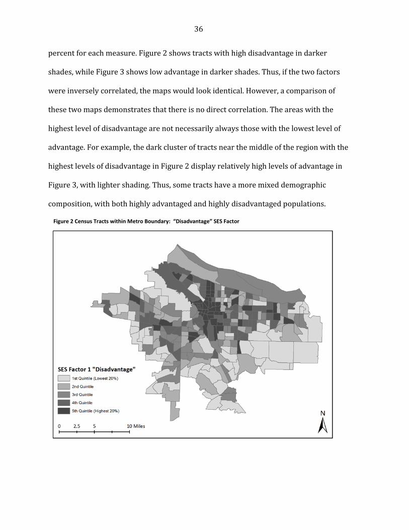
36
percent for each measure. Figure 2 shows tracts with high disadvantage in darker
shades, while Figure 3 shows low advantage in darker shades. Thus, if the two factors
were inversely correlated, the maps would look identical. However, a comparison of
these two maps demonstrates that there is no direct correlation. The areas with the
highest level of disadvantage are not necessarily always those with the lowest level of
advantage. For example, the dark cluster of tracts near the middle of the region with the
highest levels of disadvantage in Figure 2 display relatively high levels of advantage in
Figure 3, with lighter shading. Thus, some tracts have a more mixed demographic
composition, with both highly advantaged and highly disadvantaged populations.
Figure 2 Census Tracts within Metro Boundary: “Disadvantage” SES Factor
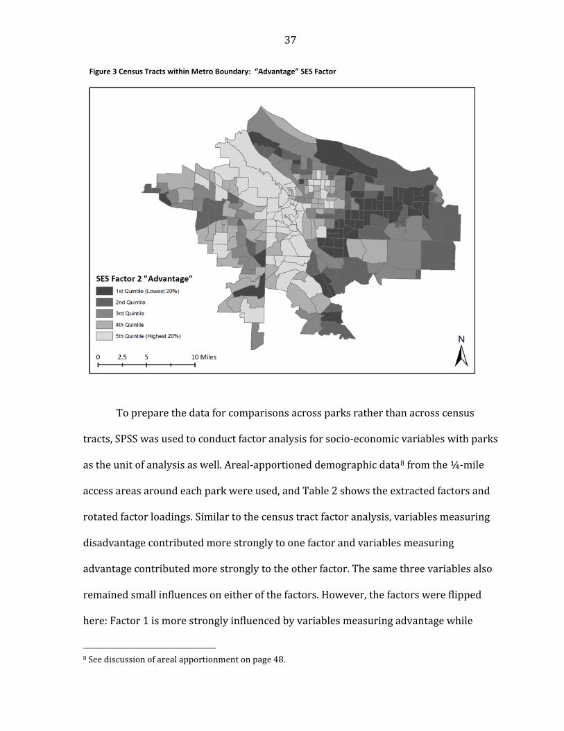
37
To prepare the data for comparisons across parks rather than across census
tracts, SPSS was used to conduct factor analysis for socio-economic variables with parks
as the unit of analysis as well. Areal-apportioned demographic data8 from the ¼-mile
access areas around each park were used, and Table 2 shows the extracted factors and
rotated factor loadings. Similar to the census tract factor analysis, variables measuring
disadvantage contributed more strongly to one factor and variables measuring
advantage contributed more strongly to the other factor. The same three variables also
remained small influences on either of the factors. However, the factors were flipped
here: Factor 1 is more strongly influenced by variables measuring advantage while
8 See discussion of areal apportionment on page 48.
Figure 3 Census Tracts within Metro Boundary: “Advantage” SES Factor

38
Factor 2 is more strongly influenced by variables measuring disadvantage. Similarly,
these two factors will be referred to as the “advantage” factor and the “disadvantage”
factor, respectively.
Table 2 Rotated Factor Matrix – ¼-mile Access Area as Unit of Analysis
Extraction Method: Principal Axis Factoring Rotation Method: Varimax with Kaiser Normalization
Factor 1 2
% With at least 4-year college degree .992 -.100
Average Household Income (in $1000s) .753 -.517
% Single female-headed household with own children under 18 -.482 .537
% White Collar .973 -.181
% Renters -.140 .773
% Below Poverty -.448 .816
% Household with no vehicle -.114 .861
% Vacancy -.048 .289
% Unemployed -.461 .622
% Non citizen -.264 .329 Bold numbers indicate the socio-economic variables that strongly influence the composition of each factor.
National Air Toxics Assessment Data
Air quality was evaluated using data from the U.S. Environmental Protection
Agency (EPA). The National-Scale Air Toxics Assessment (NATA) is a screening tool
developed by the EPA to provide a comprehensive evaluation of outdoor air toxics,
prioritize pollutants, and estimate health risks. To best maintain consistency with the
2000 Census data in this study’s analyses, the 2002 NATA was used. The 2002 NATA
provided data at the census tract level based on the 2002 National Emissions Inventory
version 3, which includes stationary emissions sources as well as on-road and non-road
mobile sources (Environmental Protection Agency 2010). NATA reports provide data in
the form of risk summaries, and for the purpose of this study, cancer and respiratory
risks were used. Carcinogens are a strong primary health concern, and respiratory risks

39
are particularly relevant to park quality, as exercise and physical activity cause
increased air intake and intensified breathing rates, which can make park users more
susceptible to poor air quality and respiratory illness.
The cancer and respiratory risks were modeled and calculated by combining
exposure concentrations with unit risk estimates and inhalation reference
concentrations (Environmental Protection Agency 2010). While concentrations of
specific air pollutants are included in each dataset, only the compiled risks were used
because this study does not require details of pollutant compounds. Cancer risks were
reported as unit risk estimates, which is the estimate of excess cancer risk over a
lifetime resulting from continuous exposure to pollutant concentrations of one
microgram per cubic meter of air (Environmental Protection Agency 2010). These are
upper-bound estimates, so the true risk is likely to be lower, although there is a small
probability the true risk could also be greater than the upper-bound estimates
(Environmental Protection Agency 2010). The average unit risk estimate for total
cancer risk of the 272 tracts is 8.3 x 10⁻⁵ per µg/m3 of air, which means that 83 excess
cancer cases are expected to develop for every 1,000,000 people with continuous
exposure over a lifetime to the total cancer sources. The cancer risks used in the
analysis were converted to cases per 1,000,000 people for simplicity.
Respiratory risks were reported as non-cancer hazard indices. These indices
represent the sum of hazard quotients (HQ) for pollutants affecting the respiratory
system (Environmental Protection Agency 2010). To calculate the hazard quotient for
pollutants, the EPA uses the inhalation reference concentration, which is an estimate of
a concentration that is unlikely to yield adverse health effects during a human’s lifetime
40
even if continuous exposure to the pollutant compound takes place. The hazard
quotient is thus a ratio of the actual exposure to this reference concentration. An HQ
less than or equal to one suggests that the exposure is not likely to yield adverse health
effects, and an HQ greater than one indicates that the exposure is greater than the
reference concentration, thus increasing the potential for adverse health effects
(Environmental Protection Agency 2010).
Although the five source categories of major source,9area source,10 on-road
mobile source,11 non-road mobile source,12 and background source13 existed for both
cancer and respiratory risk data, these were only used in the exploratory analyses of
this study. Total risk, which represented the sum of all carcinogenic risks or respiratory
hazard quotients, was used in the regression analyses.
In calculating these risks, the EPA uses population weights and exposures. Thus,
the risk estimates are influenced by human exposure modeling, which in turn is
dependent on the number of people, age and gender of the people, and human activity
within each tract (Environmental Protection Agency 2010). While inclusion of these
population weights is practical for the EPA as it prioritizes areas of high risk, the
weights are unnecessary for the purposes of this study. This study aims to examine
cancer and respiratory risks among different census tracts and parks, and already
9 Major sources refer to facilities that emit or have the potential to emit either 10 tons of any toxic air pollutant or 25 tons of more than one toxic pollutant in a year, as defined by the Clean Air Act (Environmental Protection Agency 2010). 10 Area sources include smaller facilities that do not meet the emissions thresholds of major sources, as well as wildfires and prescribed burnings (Environmental Protection Agency 2010). 11 On-road mobile sources include vehicles on roads and highways (Environmental Protection Agency 2010). 12 Non-road mobile sources include airplanes, trains, lawn mowers, farm machinery, and construction vehicles (Environmental Protection Agency 2010). 13 Background sources estimate the contributions from unidentified emissions sources, natural sources, and sources farther than 50 kilometers away (Environmental Protection Agency 2010).

41
incorporates population data by using various demographic factors as independent
variables. Therefore, the population weights were removed from the dataset for this
study.
New Spatial Variables
New spatial variables were also created for the purpose of this study, with the
aid of ArcMap geographic information systems (GIS) software. These included variables
regarding the relative geography of tracts, such as whether the tract is in the inner city
or suburban area; the number of parks within ¼-mile of tracts; and whether tracts were
considered “access” tracts based on 50% areal containment calculations, where tracts
that had at least 50% of their nonpark area within ¼-mile of at least one park were
considered tracts with park access.
Tract Geography
From preliminary analyses, the geography of the census tracts, such as whether
the tracts were in the inner city or a more suburban area, seemed to influence
demographic, air quality, and park trends. After exploring different ways to
differentiate tract geography, three categories were developed within the Metro
boundary: City of Portland tracts; major city tracts outside the City of Portland, and
suburban tracts. City of Portland tracts were those that had their centroid within
Portland city boundaries, and there were 143 tracts meeting this requirement.
For major cities, the 25 cities and towns served by Metro were examined. A
threshold population of 50,000 was selected because it is the cutoff for a city’s
designation as a Metropolitan Statistical Area (MSA) by the U.S. Census Bureau. That is,

42
if these cities existed outside of the Portland metropolitan area, each of the cities could
be individually designated as its own Metropolitan Statistical Area. With this threshold,
three cities emerged: Gresham (population: 90,205), Beaverton (population: 76,129),
and Hillsboro (population: 70,186). There were 41 tracts with their centroids within
these three major cities of Gresham, Beaverton, and Hillsboro.
Finally, the suburban tracts capture all remaining tracts in the Metro boundary.
These tracts are therefore either in smaller cities and towns that have a population less
than 50,000, or in unincorporated areas. With this designation, 88 tracts are considered
Suburban tracts. Figure 4 shows a map of these tract geographies, with labels showing
where Portland and each of the major cities are located. The single suburban tract
within Portland tracts is explained by the irregularity of the Portland city boundary.
Figure 4 Tract Geography

43
Number of Parks within ¼ Mile
Another dependent variable used to examine park access was the number of
parks that were within ¼-mile of each tract. A ¼-mile buffer was first created around
the perimeter of each park to indicate areas with reasonable park access. As a widely-
accepted metric for park access, used by the Trust for Public Land, National Recreation
and Parks Association, and the Congress for New Urbanism, a ¼-mile distance
translates to approximately 400 meters or a five-minute walk (Wolch, Wilson and
Fehrenbach 2005, Boone, et al. 2009). Although appropriate distance measurements
may vary by city, in one Portland study examining the impact of open spaces on
property values, specialists at the Metro government recommended the use of a
distance radius of around 1500 feet, or 0.28 miles, just slightly over the ¼-mile
threshold (Bolitzer and Netusil 2000).
As opposed to performing distance-based analyses from the centroid of a facility
or a point, as is common in the study of toxic waste facilities (Mohai and Saha 2006,
Bullard, et al. 2007), some park analyses create a distance buffer from the edge of the
park (Boone, et al. 2009). By treating parks as a two-dimensional space, any point along
the park perimeter can be treated as the destination point (Boone, et al. 2009, Wolch,
Wilson and Fehrenbach 2005). This assumes that access along park perimeters is not
blocked by fences, roads, or private property. Furthermore, in suburban tracts where
streets do not tend to follow straight gridline patterns, there may be additional error
associated with this approach (Boone, et al. 2009). As demonstrated by the many
studies that have used this simplifying assumption, however, this approach is
reasonable and well-supported.
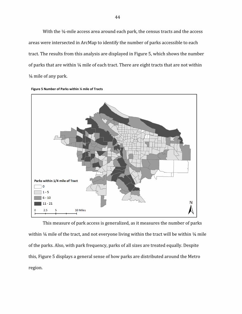
44
With the ¼-mile access area around each park, the census tracts and the access
areas were intersected in ArcMap to identify the number of parks accessible to each
tract. The results from this analysis are displayed in Figure 5, which shows the number
of parks that are within ¼ mile of each tract. There are eight tracts that are not within
¼ mile of any park.
This measure of park access is generalized, as it measures the number of parks
within ¼ mile of the tract, and not everyone living within the tract will be within ¼ mile
of the parks. Also, with park frequency, parks of all sizes are treated equally. Despite
this, Figure 5 displays a general sense of how parks are distributed around the Metro
region.
Figure 5 Number of Parks within ¼ mile of Tracts
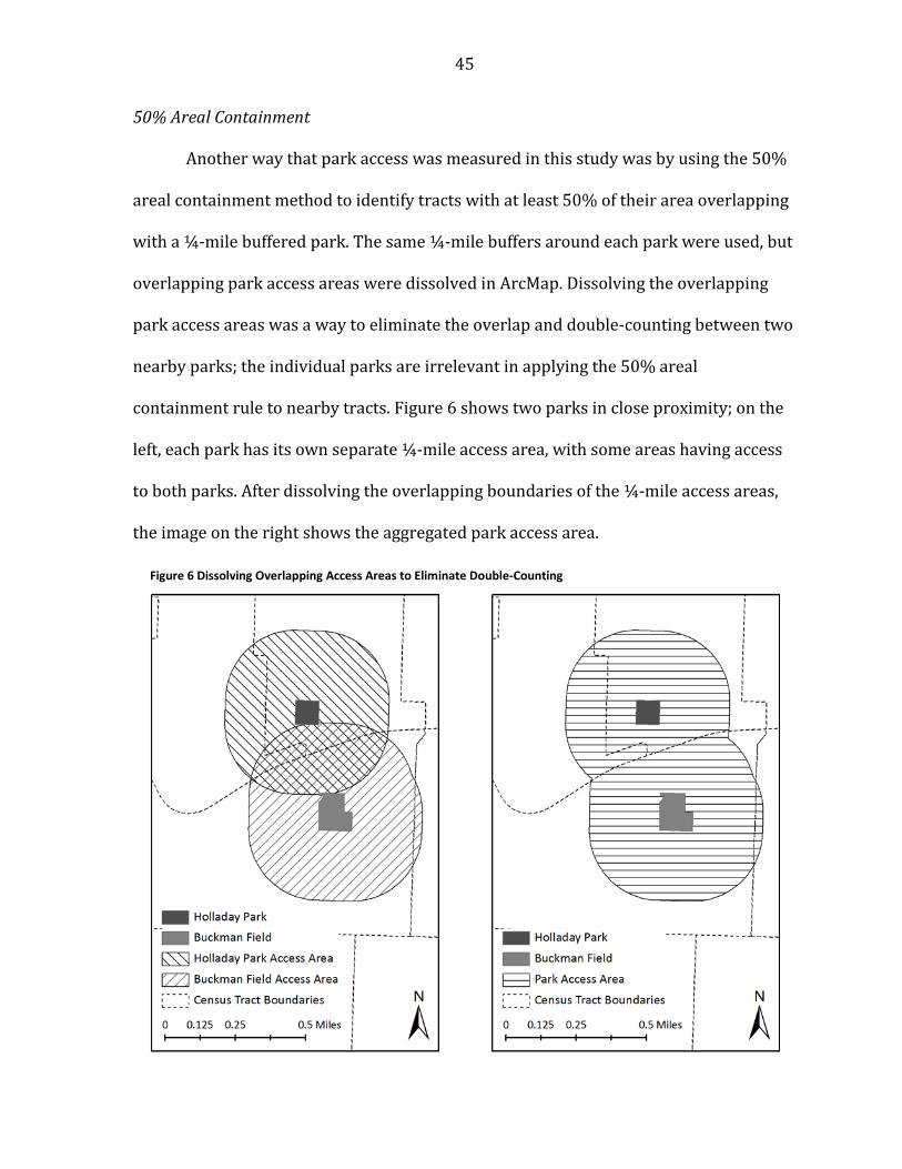
45
50% Areal Containment
Another way that park access was measured in this study was by using the 50%
areal containment method to identify tracts with at least 50% of their area overlapping
with a ¼-mile buffered park. The same ¼-mile buffers around each park were used, but
overlapping park access areas were dissolved in ArcMap. Dissolving the overlapping
park access areas was a way to eliminate the overlap and double-counting between two
nearby parks; the individual parks are irrelevant in applying the 50% areal
containment rule to nearby tracts. Figure 6 shows two parks in close proximity; on the
left, each park has its own separate ¼-mile access area, with some areas having access
to both parks. After dissolving the overlapping boundaries of the ¼-mile access areas,
the image on the right shows the aggregated park access area.
Figure 6 Dissolving Overlapping Access Areas to Eliminate Double-Counting
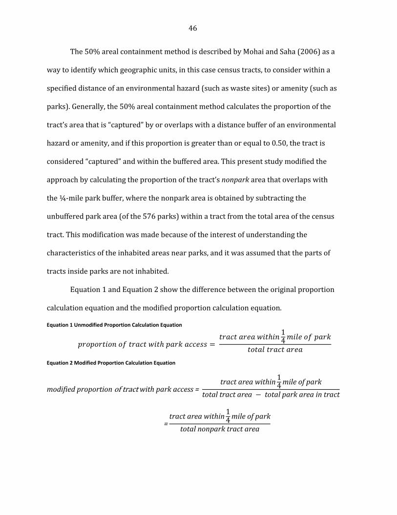
46
The 50% areal containment method is described by Mohai and Saha (2006) as a
way to identify which geographic units, in this case census tracts, to consider within a
specified distance of an environmental hazard (such as waste sites) or amenity (such as
parks). Generally, the 50% areal containment method calculates the proportion of the
tract’s area that is “captured” by or overlaps with a distance buffer of an environmental
hazard or amenity, and if this proportion is greater than or equal to 0.50, the tract is
considered “captured” and within the buffered area. This present study modified the
approach by calculating the proportion of the tract’s nonpark area that overlaps with
the ¼-mile park buffer, where the nonpark area is obtained by subtracting the
unbuffered park area (of the 576 parks) within a tract from the total area of the census
tract. This modification was made because of the interest of understanding the
characteristics of the inhabited areas near parks, and it was assumed that the parts of
tracts inside parks are not inhabited.
Equation 1 and Equation 2 show the difference between the original proportion
calculation equation and the modified proportion calculation equation.
Equation 1 Unmodified Proportion Calculation Equation
𝑝𝑟𝑜𝑝𝑜𝑟𝑡𝑖𝑜𝑛 𝑜𝑓 𝑡𝑟𝑎𝑐𝑡 𝑤𝑖𝑡ℎ 𝑝𝑎𝑟𝑘 𝑎𝑐𝑐𝑒𝑠𝑠 = 𝑡𝑟𝑎𝑐𝑡 𝑎𝑟𝑒𝑎 𝑤𝑖𝑡ℎ𝑖𝑛 1
4𝑚𝑖𝑙𝑒 𝑜𝑓 𝑝𝑎𝑟𝑘𝑡𝑜𝑡𝑎𝑙 𝑡𝑟𝑎𝑐𝑡 𝑎𝑟𝑒𝑎
Equation 2 Modified Proportion Calculation Equation
modified proportion of tract with park access = tract area within 1
4 mile of parktotal tract area − total park area in tract
=tract area within 1
4 mile of parktotal nonpark tract area
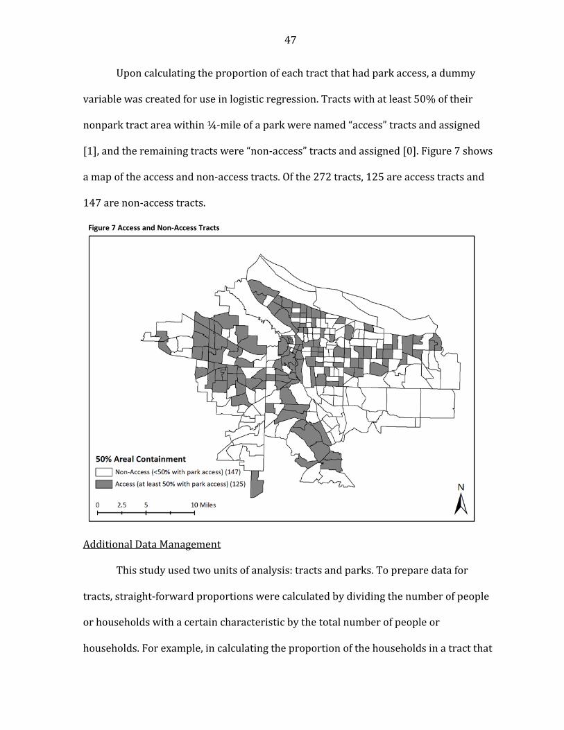
47
Upon calculating the proportion of each tract that had park access, a dummy
variable was created for use in logistic regression. Tracts with at least 50% of their
nonpark tract area within ¼-mile of a park were named “access” tracts and assigned
[1], and the remaining tracts were “non-access” tracts and assigned [0]. Figure 7 shows
a map of the access and non-access tracts. Of the 272 tracts, 125 are access tracts and
147 are non-access tracts.
Additional Data Management
This study used two units of analysis: tracts and parks. To prepare data for
tracts, straight-forward proportions were calculated by dividing the number of people
or households with a certain characteristic by the total number of people or
households. For example, in calculating the proportion of the households in a tract that
Figure 7 Access and Non-Access Tracts

48
were renters, the number of renter-occupied units were divided by the total number of
occupied housing units. In some cases, the total population in the denominator was not
the total population of the tract, as the proportion of people with at least a four-year
college degree included only those over the age of 25 in the denominator (See Appendix
B - Table 4).
For parks as the unit of analysis, however, the data required further preparation.
The data associated with parks are grouped into two categories: those that pertain to
the park area itself as the geographic unit, and those that pertain to the ¼-mile access
area around the park as the geographic unit. NATA data were applied to just the park
area itself, as this study aimed to examine the cancer and respiratory risks within parks.
However, because of the assumption that no people live in parks, demographic data
were applied only to the ¼-mile access areas around the parks. This access area
excluded the area of the park, and can thus be considered as a ¼-mile-wide ring around
each park. Figure 8 illustrates an example of a park with its associated ¼-mile access
area.
Areal Apportionment
As evident in Figure 8, the geographic units do not line up with census tract
boundaries when parks are the unit of analysis. Therefore, areal apportionment was
used to estimate the characteristics of the parks and ¼-mile access areas around them.
In ArcMap, the parks and ¼-mile access areas were intersected with the underlying
census tract boundaries that contained demographic and NATA data in preparation for
areal apportionment calculations.

49
The areal apportionment method uses a weighting scheme to perform distance-
based analyses. Demographic characteristics of each census tract contained by or
intersecting with ¼-mile access areas are aggregated based on the proportion of the
area of each tract within the access area (Mohai and Saha 2006). Specifically, the
proportion of the area of each tract that is intersected by the ¼-mile access area is
assumed to be equal to the proportion of the population of each tract that is within the
access area. Similar to the modifications made to the 50% areal containment method,
Mohai and Saha’s (2006) areal apportionment techniques were adapted to this present
study by using the nonpark tract area, as displayed in Equation 3.
Figure 8 Park and its 1/4-Mile Access Area

50
Equation 3 Areal Apportionment Calculation for Demographic Characteristics
𝐷 =∑ (𝑎𝑖/𝐴𝑖)(𝑝𝑖)(𝑑𝑖)𝑛𝑖=1∑ (𝑎𝑖/𝐴𝑖)(𝑝𝑖)𝑛𝑖=1
D = demographic characteristics of the ¼-mile access area (e.g. proportion of renters in the access area) ai = area of tract i within the ¼-mile access area Ai = total nonpark area of tract i pi = total population of tract i di = demographic characteristics in tract i (e.g. proportion of renters in tract i) n = number of tracts within the ¼-mile access area
Since the Census reports numbers rather than proportions, the product of pi and di
could be replaced by the number of people displaying the specific characteristic (e.g. the
number of renters in tract i).
For the NATA data, however, the cancer and respiratory risks are uniform across
the census tracts. Multiplying the proportion of the tract that is within the park by the
cancer or respiratory risks would not be appropriate, and thus a different approach was
necessary. The contribution of each tract to the park was still weighted, but rather than
using the proportion of tract area that is within the park, the relative contributions of
each tract to the park were calculated. This ends up being a weighted average, and the
resulting cancer or respiratory risks of the park should be within the range of the risks
of the contributing tracts. Equation 4 shows the equation for calculating the weighted
average of cancer or respiratory risks within the park using the tract-level cancer and
respiratory risk estimates.

51
Equation 4 Weighted Average Calculation for NATA Data
𝑅 = �(𝑘𝑖/𝐾)(𝑟𝑖)𝑛
𝑖=1
R = cancer or respiratory risk of the park ki = proportion of the park area within tract i K = total park area ri = cancer or respiratory risk of tract i n = number of tracts within the park
After performing the areal apportionment and proportion calculations for both
tracts and parks as the units of analysis, the data were prepared for regression analyses.
Regression Analyses
Regression analyses were performed on both tracts and parks as the units of
analysis. For tracts as the unit of analysis, logistic regression was used when the
dichotomous “access/non-access tracts” variable was the dependent variable. Also for
tracts as the unit of analysis, multiple linear regression was used to predict total cancer
risk of the tract, total respiratory risk of the tract, and the number of parks within ¼
mile of a tract. For each dependent variable in the regression analyses for tracts as the
unit of analysis, four regressions were run. The first regression included all 272 census
tracts, and the remaining three focused on each tract geography separately. Thus, the
regressions were run for just Portland tracts, just major city tracts, and just suburban
tracts.
When examining parks as the unit of analysis, the total cancer and respiratory
risks of parks served as the dependent variables in the multiple linear regression
analyses. Preliminary analyses explored park area as both a dependent and an

52
independent variable, but the final analyses do not include park area due to its lack of
statistical significance. With parks as the unit of analysis, the independent demographic
variables were calculated for the ¼-mile access areas around each park.
For both units of analysis, the independent variables were introduced to the
model in groups. In the environmental justice field, a common question regards
whether race is a significant predictor of environmental inequalities, with and without
control for socio-economic variables. Thus, racial/ethnic variables were included in the
model first, and the two socio-economic factors extracted from factor analysis were
added as a second step. Also, given the racial/ethnic demographics of the Portland
study area, where the minority population is relatively small, two versions of the
regressions were run: one with an aggregate “People of Color” variable, and another
with the three largest minority groups of black, Asian, and Hispanic. Black Hispanics
and Asian Hispanics were removed from the Hispanic category to ensure that the
categories did not overlap. The regression analyses were run in SPSS, and an alpha
value of 0.05 was used to determine statistical significance of the odds ratios,
standardized betas, and R2 values.
Census Tracts as Unit of Analysis
To determine whether the racial/ethnic and socio-economic characteristics help
predict the likelihood of a tract being an access tract according to the modified 50%
areal containment calculations, a logistic regression was used. The dependent variable
was a dummy variable, with [0] representing tracts with less than 50% of their nonpark
tract area within ¼ mile of a park, and [1] representing tracts with at least 50% of their
nonpark tract area within ¼ mile of a park. With this dependent variable, four

53
regression analyses were run, one for each of the tract geographies and one for all 272
tracts. Within each regression, four models were generated to account for the
aggregated and disaggregated racial/ethnic variables and the inclusion of the socio-
economic variables. Due to skewness in the distribution of demographic values, the
racial/ethnic dummy variables were used in the logistic regression rather than actual
percentages of people in each of the racial/ethnic categories.
Dependent variables also included the cancer and respiratory risks, as well as
the number of parks within ¼ mile of the tract. Bivariate correlations among the
dependent and independent demographic variables were examined. Then, multiple
linear regressions were run following the procedures above, with four regressions per
dependent variable, and four models per regression. When doing the regressions for the
number of parks within ¼ mile of the tract, only the 125 access tracts based on the 50%
areal containment method were used in the analysis.
Parks as Unit of Analysis
Park area was first explored as a dependent variable for a regression analyses
with racial/ethnic and socio-economic independent variables, but none of the
independent variables were statistically significant. The role of park area in
ameliorating cancer and respiratory risks was also explored, and park area was used as
an independent variable in the multiple linear regression analyses for total cancer and
respiratory risks of parks. Again, no statistical significance emerged. Thus, the focus for
parks as the unit of analysis was on the cancer and respiratory risks of parks. As the
parks were not separated into geographies, only one regression was run for each
dependent variable. However, the stepping procedures, with racial/ethnic variables
54
entering the model before the socio-economic variables, were consistent with the
procedures used in the regressions for tracts.
In summary, this chapter discussed the details of data preparation and
management, as well as the procedures followed in regression analyses. After the
regression analyses were performed, results from the regressions were examined. The
next chapter presents the results from the regression analyses.

55
CHAPTER FOUR - RESULTS
Tracts as Unit of Analysis
Access Tracts: 50% Containment
To better understand the racial/ethnic composition of non-access vs. access
tracts, bar graphs of both the raw population numbers and the population proportions
were created. Figure 9 shows aggregated population numbers and displays the sum of
all people within each racial/ethnic group for all non-access and access tracts. It shows
that as a whole, more people live in non-access tracts than in access tracts. However,
more people of color live in access tracts, and this holds true even when people of color
are disaggregated into the three primary racial/ethnic categories in the area.
Figure 10 shows the percentage of the aggregated population within each
racial/ethnic category that lives in non-access versus access tracts, and it displays the
same information as Figure 9, but with percentages. Again, of all people of color, a
higher percentage lives in access tracts than in non-access tracts, and the opposite is
true for the white population. Although Figure 10 shows the same basic information as
Figure 9, the relative proportions in non-access and access tracts within each
racial/ethnic group in Figure 10 helps clarify the trend, since the population numbers
vary widely across racial/ethnic groups. The logistic regressions also similarly
demonstrate these trends, and each regression table will be presented in the following
pages.
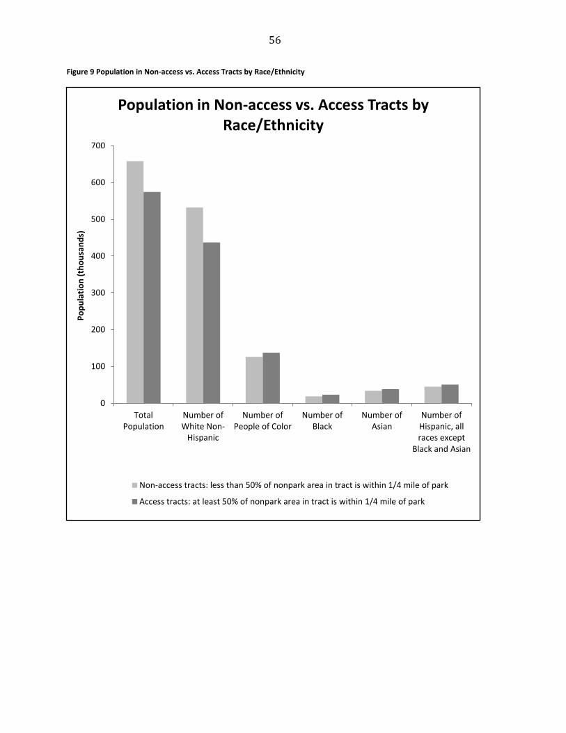
56
Figure 9 Population in Non-access vs. Access Tracts by Race/Ethnicity
0
100
200
300
400
500
600
700
TotalPopulation
Number ofWhite Non-
Hispanic
Number ofPeople of Color
Number ofBlack
Number ofAsian
Number ofHispanic, allraces except
Black and Asian
Popu
latio
n (t
hous
ands
)
Population in Non-access vs. Access Tracts by Race/Ethnicity
Non-access tracts: less than 50% of nonpark area in tract is within 1/4 mile of park
Access tracts: at least 50% of nonpark area in tract is within 1/4 mile of park
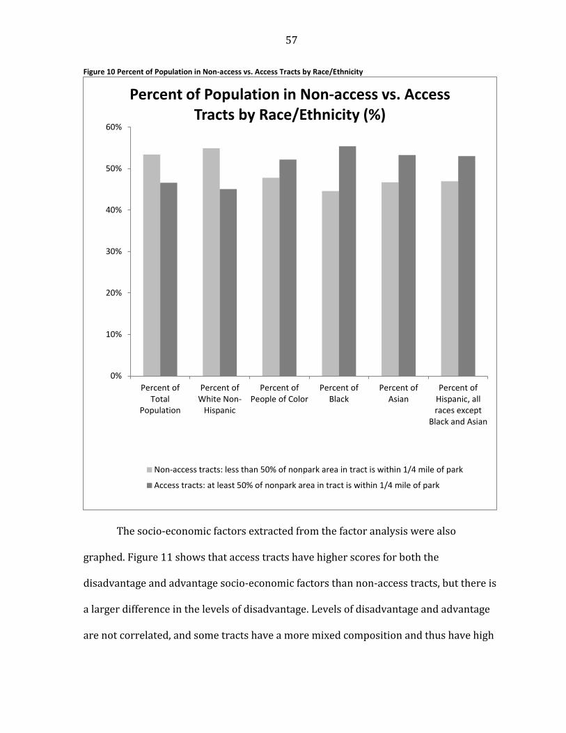
57
Figure 10 Percent of Population in Non-access vs. Access Tracts by Race/Ethnicity
The socio-economic factors extracted from the factor analysis were also
graphed. Figure 11 shows that access tracts have higher scores for both the
disadvantage and advantage socio-economic factors than non-access tracts, but there is
a larger difference in the levels of disadvantage. Levels of disadvantage and advantage
are not correlated, and some tracts have a more mixed composition and thus have high
0%
10%
20%
30%
40%
50%
60%
Percent ofTotal
Population
Percent ofWhite Non-
Hispanic
Percent ofPeople of Color
Percent ofBlack
Percent ofAsian
Percent ofHispanic, allraces except
Black and Asian
Percent of Population in Non-access vs. Access Tracts by Race/Ethnicity (%)
Non-access tracts: less than 50% of nonpark area in tract is within 1/4 mile of park
Access tracts: at least 50% of nonpark area in tract is within 1/4 mile of park

58
levels of both advantage and disadvantage (See Figure 2 and Figure 3). The trends in
the graph are displayed in the logistic regression analyses as well.
Figure 11 Average SES Factor Scores in Non-access vs. Access Tracts
-0.2
-0.15
-0.1
-0.05
0
0.05
0.1
0.15
0.2
Disadvantage Advantage
Average Disadvantage and Advantage Factor Scores in Non-access vs. Access Tracts
Non-access tracts: less than 50%of nonpark area in tract is within1/4 mile of park
Access tracts: at least 50% ofnonpark area in tract is within1/4 mile of park
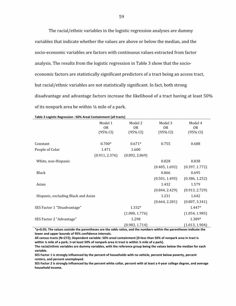
59
The racial/ethnic variables in the logistic regression analyses are dummy
variables that indicate whether the values are above or below the median, and the
socio-economic variables are factors with continuous values extracted from factor
analysis. The results from the logistic regression in Table 3 show that the socio-
economic factors are statistically significant predictors of a tract being an access tract,
but racial/ethnic variables are not statistically significant. In fact, both strong
disadvantage and advantage factors increase the likelihood of a tract having at least 50%
of its nonpark area be within ¼ mile of a park.
Table 3 Logistic Regression –50% Areal Containment [all tracts]
Model 1 OR
(95% CI)
Model 2 OR
(95% CI)
Model 3 OR
(95% CI)
Model 4 OR
(95% CI)
Constant 0.700* 0.671* 0.755 0.688 People of Color 1.471 1.600
(0.911, 2.376) (0.892, 2.869) White, non-Hispanic
0.828 0.838
(0.405, 1.692) (0.397, 1.772)
Black
0.866 0.695
(0.501, 1.495) (0.386, 1.252)
Asian
1.432 1.579
(0.844, 2.429) (0.913, 2.729)
Hispanic, excluding Black and Asian
1.231 1.642
(0.664, 2.281) (0.807, 3.341)
SES Factor 1 "Disadvantage"
1.332*
1.447*
(1.000, 1.776)
(1.054, 1.985)
SES Factor 2 "Advantage"
1.298
1.389*
(0.983, 1.714)
(1.013, 1.904)
*p<0.05; The values outside the parentheses are the odds ratios, and the numbers within the parentheses indicate the lower and upper bounds of 95% confidence intervals. All census tracts (N=272); Dependent variable: 50% areal containment [0=less than 50% of nonpark area in tract is within ¼ mile of a park; 1=at least 50% of nonpark area in tract is within ¼ mile of a park]. The racial/ethnic variables are dummy variables, with the reference group being the values below the median for each variable. SES Factor 1 is strongly influenced by the percent of households with no vehicle, percent below poverty, percent renters, and percent unemployed. SES Factor 2 is strongly influenced by the percent white collar, percent with at least a 4-year college degree, and average household income.

60
With only the City of Portland tracts, Table 4 shows that no variables are
statistically significant in predicting a tract being an access tract or a non-access tract.
Table 4 Logistic Regression –50% Areal Containment [Portland]
Model 1 OR
(95% CI)
Model 2 OR
(95% CI)
Model 3 OR
(95% CI)
Model 4 OR
(95% CI)
Constant 0.966 0.948 0.900 0.858 People of Color 1.036 0.919
(0.530, 2.023) (0.337, 2.504) White, non-Hispanic
1.261 1.292
(0.430, 3.705) (0.403, 4.141)
Black
0.830 0.698
(0.377, 1.832) (0.301, 1.616)
Asian
0.727 0.804
(0.358, 1.478) (0.367, 1.763)
Hispanic, excluding Black and Asian
1.800 1.784
(0.685, 4.732) (0.616, 5.166)
SES Factor 1 "Disadvantage"
1.293
1.310
(0.936, 1.786)
(0.930, 1.844)
SES Factor 2 "Advantage"
0.987
1.016
(0.640, 1.522)
(0.610, 1.695)
*p<0.05; The values outside the parentheses are the odds ratios, and the numbers within the parentheses indicate the lower and upper bounds of 95% confidence intervals. Only tracts within Portland city limits (N=143); Dependent variable: 50% areal containment [0=less than 50% of nonpark in tract is within ¼ mile of a park; 1=at least 50% of nonpark area in tract is within ¼ mile of a park]. The racial/ethnic variables are dummy variables, with the reference group being the values below the median for each variable. SES Factor 1 is strongly influenced by the percent of households with no vehicle, percent below poverty, percent renters, and percent unemployed. SES Factor 2 is strongly influenced by the percent white collar, percent with at least a 4-year college degree, and average household income.
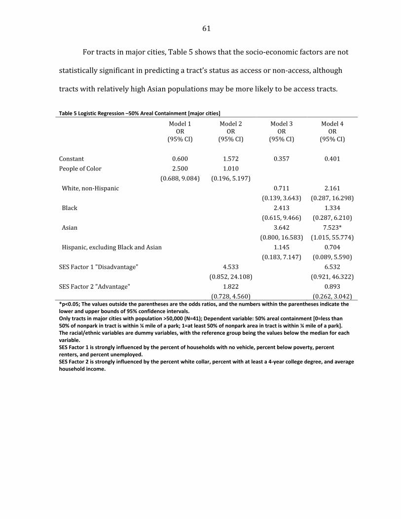
61
For tracts in major cities, Table 5 shows that the socio-economic factors are not
statistically significant in predicting a tract’s status as access or non-access, although
tracts with relatively high Asian populations may be more likely to be access tracts.
Table 5 Logistic Regression –50% Areal Containment [major cities]
Model 1 OR
(95% CI)
Model 2 OR
(95% CI)
Model 3 OR
(95% CI)
Model 4 OR
(95% CI)
Constant 0.600 1.572 0.357 0.401 People of Color 2.500 1.010
(0.688, 9.084) (0.196, 5.197) White, non-Hispanic
0.711 2.161
(0.139, 3.643) (0.287, 16.298)
Black
2.413 1.334
(0.615, 9.466) (0.287, 6.210)
Asian
3.642 7.523*
(0.800, 16.583) (1.015, 55.774)
Hispanic, excluding Black and Asian
1.145 0.704
(0.183, 7.147) (0.089, 5.590)
SES Factor 1 "Disadvantage"
4.533
6.532
(0.852, 24.108)
(0.921, 46.322)
SES Factor 2 "Advantage"
1.822
0.893
(0.728, 4.560)
(0.262, 3.042)
*p<0.05; The values outside the parentheses are the odds ratios, and the numbers within the parentheses indicate the lower and upper bounds of 95% confidence intervals. Only tracts in major cities with population >50,000 (N=41); Dependent variable: 50% areal containment [0=less than 50% of nonpark in tract is within ¼ mile of a park; 1=at least 50% of nonpark area in tract is within ¼ mile of a park]. The racial/ethnic variables are dummy variables, with the reference group being the values below the median for each variable. SES Factor 1 is strongly influenced by the percent of households with no vehicle, percent below poverty, percent renters, and percent unemployed. SES Factor 2 is strongly influenced by the percent white collar, percent with at least a 4-year college degree, and average household income.

62
For suburban tracts, Table 6 shows that the only statistically significant variable
in the regression is the dummy variable for the black population. Thus, tracts that have
an above-median percentage of blacks have a lower likelihood of being an access tract.
Table 6 Logistic Regression –50% Areal Containment [suburban]
Model 1 OR
(95% CI)
Model 2 OR
(95% CI)
Model 3 OR
(95% CI)
Model 4 OR
(95% CI)
Constant 0.537* 0.640 0.473 0.634 People of Color 1.464 1.643
(0.569, 3.765) (0.580, 4.658) White, non-Hispanic
0.895 0.798
(0.187, 4.286) (0.160, 3.988)
Black
0.180* 0.191*
(0.043, 0.744) (0.046, 0.785)
Asian
3.610* 2.658
(1.154, 11.290) (0.782, 9.033)
Hispanic, excluding Black and Asian
1.492 1.842
(0.460, 4.842) (0.487, 6.964)
SES Factor 1 "Disadvantage"
1.526
1.404
(0.467, 4.987)
(0.365, 5.405)
SES Factor 2 "Advantage"
1.884*
1.692
(1.082, 3.280)
(0.883, 3.242)
*p<0.05; The values outside the parentheses are the odds ratios, and the numbers within the parentheses indicate the lower and upper bounds of 95% confidence intervals. Only tracts in suburbs (N=88); Dependent variable: 50% areal containment [0=less than 50% of nonpark in tract is within ¼ mile of a park; 1=at least 50% of nonpark area in tract is within ¼ mile of a park]. The racial/ethnic variables are dummy variables, with the reference group being the values below the median for each variable. SES Factor 1 is strongly influenced by the percent of households with no vehicle, percent below poverty, percent renters, and percent unemployed. SES Factor 2 is strongly influenced by the percent white collar, percent with at least a 4-year college degree, and average household income.
63
Bivariate Correlations: Tracts
Next, bivariate correlations were examined between the independent
demographic variables and the dependent variables of tract cancer risk, tract
respiratory risk, and number of parks within ¼-mile of the tracts. Table 7 shows the
Pearson correlation coefficients among the independent and dependent variables used
in the linear regression analyses with tract as the unit of analysis, for all 272 tracts in
the study area. Some particularly strong correlations include the positive correlation
between total respiratory risk and the disadvantage socio-economic factor, and
between the total cancer and respiratory risks. Also, total cancer risk and the percent
people of color are both positively correlated with the disadvantage socio-economic
factor. The percent people of color and the percent Hispanic variables are also
negatively correlated with the advantage socio-economic factor. With the statistically
significant correlations, regression analyses can help the understanding of these
relationships.

64
Table 7 Bivariate Correlations for Demographic and Tract Variables
Pearson Correlations % People of Color
% Black
% Asian
% Hispanic excluding Blacks and Asians
SES Factor 1 "Disadvantage"
SES Factor 2 "Advantage"
Total Cancer Risk
Total Respiratory Risk
Number of parks within 1/4 mile of tract
% People of Color 1 .757* .228* .617* .430* -.420* .081 .178* -.203** % Black .757* 1 -.128* .108 .396* -.134* .177* .253* -.224* % Asian .228* -.128* 1 -.037 -.012 .002 -.102 -.004 .159* % Hispanic excluding Blacks and Asians .617* .108 -.037 1 .211** -.509* -.046 -.042 -.114
SES Factor 1 “Disadvantage" .430* .396* -.012 .211* 1 -.015 .491* .738* -.272*
SES Factor 2 "Advantage" -.420* -.134* .002 -.509* -.015 1 -.039 .162* .281* Total Cancer Risk .081 .177* -.102 -.046 .491* -.039 1 .695* -.333* Total Respiratory Risk .178* .253* -.004 -.042 .738* .162* .695* 1 -.333* Number of parks within 1/4 mile of tract -.203* -.224* .159* -.114 -.272* .281* -.333* -.333* 1 *p<0.05; All census tracts (N=272) SES Factor 1 [unit of analysis: tracts] is strongly influenced by the percent of households with no vehicle, percent of population below poverty, percent renters, and percent unemployed. SES Factor 2 [unit of analysis: tracts] is strongly influenced by the percent white collar, percent with at least a 4-year college degree, and average household income.
65
Total Cancer Risk of Tract
Table 8 shows that the higher the percentage of people of color, the lower the
cancer risk in a tract. In the bivariate correlations (Table 7), the percent people of color
and cancer risk is not statistically significant, and this negative and statistically
significant relationship between percent people of color and cancer risk results only
when applying multivariate controls for socio-economic status. However, when people
of color are separated, the Asian and Hispanic populations are the ones that are more
significantly driving this negative correlation (Model 4).
The disadvantage socio-economic factor is positively correlated and the
advantage factor is negatively correlated with cancer risk, regardless of how the
racial/ethnic variables are aggregated. Since the disadvantage factor is strongly
influenced by percent of households with no vehicle, percent below poverty, percent
renters, and percent unemployed, the greater the percentage for each of these variables,
the greater the total cancer risk of the census tract. The advantage factor is strongly
influenced by percent white collar, percent with at least a 4-year college degree, and
average household income, so the regression results suggest that with higher
percentages for these variables, the total cancer risk in the census tract decreases.
Overall, the influence of the socio-economic variables is stronger than that of the
racial/ethnic variables in the regression models, demonstrating the influence of socio-
economic status of tract residents on the cancer risks of the tract.

66
Table 8 Linear Regression –Total Tract Cancer Risk [all tracts]
*p<0.05; The beta estimates for the constants in the linear regression tables are not standardized. All census tracts (N=272); Dependent variable: Total cancer risk of census tract. SES Factor 1 is strongly influenced by the percent of households with no vehicle, percent of population below poverty, percent renters, and percent unemployed. SES Factor 2 is strongly influenced by the percent white collar, percent with at least a 4-year college degree, and average household income.
Model 1 Model 2 Model 3 Model 4
Std. Beta
Sig. VIF Std. Beta
Sig. VIF Std. Beta
Sig. VIF Std. Beta
Sig. VIF
Constant 79.185* .000
3.993* .000
86.979* .000
98.475* .000 % People of Color 0.081 .181 1.00 -0.221* .001 1.55
% Black
0.174* .004 1.03 -0.054 .346 1.24 % Asian
-0.083 .171 1.02 -0.111* .033 1.02
% Hispanic, excluding Black and Asian
-0.068 .259 1.01 -0.245* .000 1.44
SES Factor 1 "Disadvantage"
0.584* .000 1.28
0.560* .000 1.26 SES Factor 2 "Advantage"
-0.123* .036 1.27
-0.162* .008 1.40
Adjusted R2 .003 .266* .032* .281*
67
For tracts within Portland city limits, Table 9 shows that the only demographic
variable that is significantly correlated with total cancer risk is the disadvantage socio-
economic factor. The greater the percentage of households with no vehicle, people
below poverty, renters, and unemployed, the higher the total cancer risk of the census
tract.

68
Table 9 Linear Regression –Total Tract Cancer Risk [Portland]
Model 1 Model 2 Model 3 Model 4
Std. Beta
Sig. VIF Std. Beta
Sig. VIF Std. Beta
Sig. VIF Std. Beta
Sig. VIF
Constant 90.048* .000
4.895* .000
95.522* .000
94.033* .000 % People of Color 0.066 .434 1.00 -0.120 .170 1.66
% Black
0.095 .313 1.24 -0.075 .346 1.37 % Asian
-0.059 .512 1.13 -0.034 .675 1.41
% Hispanic, excluding Black and Asian
-0.024 .789 1.16 -0.084 .374 1.94
SES Factor 1 "Disadvantage"
0.633* .000 1.15
0.630* .000 1.14 SES Factor 2 "Advantage"
0.006 .944 1.51
-0.012 .906 2.24
Adjusted R2 -.003 .357* -.006 .348* *p<0.05; The beta estimates for the constants in the linear regression tables are not standardized. Only tracts within Portland city limits (N=143); Dependent variable: Total cancer risk of census tract. SES Factor 1 is strongly influenced by the percent of households with no vehicle, percent of population below poverty, percent renters, and percent unemployed. SES Factor 2 is strongly influenced by the percent white collar, percent with at least a 4-year college degree, and average household income.

69
Table 10 displays results for the tracts within the major cities of Beaverton,
Gresham, and Hillsboro, where the percentage of the black population is positively
correlated with total cancer risk, but the significance of the correlation disappears
when the socio-economic factors are introduced. Within these major cities, neither
race/ethnicity nor socio-economic variables seem to be predictive of cancer risk in
census tracts.

70
Table 10 Linear Regression –Total Tract Cancer Risk [major cities]
Model 1 Model 2 Model 3 Model 4
Std. Beta
Sig. VIF Std. Beta
Sig. VIF Std. Beta
Sig. VIF Std. Beta
Sig. VIF
Constant 58.017* .000
5.921* .000
58.061* .000
62.623* .000 % People of Color 0.199 .212 1.00 -0.133 .562 2.24
% Black
0.345* .034 1.08 0.227 .273 1.77 % Asian
-0.102 .530 1.14 -0.148 .526 2.26
% Hispanic, excluding Black and Asian
0.076 .653 1.21 -0.076 .747 2.33
SES Factor 1 "Disadvantage"
0.423 .083 2.42
0.260 .324 2.92 SES Factor 2 "Advantage"
-0.086 .598 1.14
0.013 .958 2.62
Adjusted R2 .015 .070 .083 .058 *p<0.05; The beta estimates for the constants in the linear regression tables are not standardized. Only tracts in major cities with population >50,000 (N=41); Dependent variable: Total cancer risk of census tract. SES Factor 1 is strongly influenced by the percent of households with no vehicle, percent of population below poverty, percent renters, and percent unemployed. SES Factor 2 is strongly influenced by the percent white collar, percent with at least a 4-year college degree, and average household income.
71
In looking at the tracts beyond the major cities and Portland, Table 11 shows
that socio-economic factors are significantly correlated with the total cancer risk of the
census tract in the expected directions. The greater the disadvantaged population, the
higher the total cancer risk. The smaller the advantaged population, the higher the total
cancer risk. This shows the strong effect of socio-economic status on the cancer risk of
suburban tracts, as the coefficients for the socio-economic factors are not only
statistically significant, but also larger relative to the coefficients of the racial/ethnic
variables. The percent people of color is negatively correlated with the total cancer risk
only when socio-economic factors are introduced to the model (Model 2). However,
when the percent people of color is separated into racial/ethnic groups, only the socio-
economic factors are significant predictors of total cancer risk.

72
Table 11 Linear Regression –Total Tract Cancer Risk [suburban]
Model 1 Model 2 Model 3 Model 4 Std. Beta
Sig. VIF Std. Beta
Sig. VIF Std. Beta
Sig. VIF Std. Beta Sig. VIF
Constant 78.851* .000
12.435* .000
80.143* .000
106.496* .000 % People of Color -0.016 .886 1.00 -0.245* .033 1.37
% Black
0.040 .708 1.04 -0.066 .526 1.11 % Asian
-0.226* .038 1.03 -0.042 .712 1.31
% Hispanic, excluding Black and Asian
0.147 .174 1.03 -0.236 .100 2.10
SES Factor 1 "Disadvantage"
0.276* .016 1.35
0.302* .018 1.63 SES Factor 2 "Advantage"
-0.389* .000 1.07
-0.432* .001 1.67
Adjusted R2
-.011
.191*
.033
.166* *p<0.05; The beta estimates for the constants in the linear regression tables are not standardized.
Only tracts in suburbs (N=88); Dependent variable: Total cancer risk of census tract. SES Factor 1 is strongly influenced by the percent of households with no vehicle, percent of population below poverty, percent renters, and percent unemployed. SES Factor 2 is strongly influenced by the percent white collar, percent with at least a 4-year college degree, and average household income.

73
Total Respiratory Risk of Tract
For respiratory risk, the strongest driver in the regression model is the
disadvantage socio-economic status factor, as evidenced by the statistically significant
and much larger coefficient relative to those of the other independent variables (See
Table 12). Although the percent people of color has a positive and statistically
significant bivariate correlation with the total respiratory risk of a census tract, this
coefficient becomes negative and statistically significant with the inclusion of socio-
economic variables. This further demonstrates the strong influence of the socio-
economic factors, as the results suggest that race/ethnicity may ameliorate some of the
strong positive correlation between disadvantaged socio-economic status and
respiratory risk. The advantage socio-economic factor is also positive and statistically
significant in Model 2, but the coefficient is much smaller than that of the disadvantage
socio-economic factor.
When people of color are separated into subcategories in Model 3 and Model 4,
the disadvantage socio-economic factor still displays a large positive and statistically
significant coefficient. For racial/ethnic variables, the percent black displays the same
pattern as the overall percent people of color, as the coefficient becomes negative with
the introduction of socio-economic variables. The Hispanic population has a negative
coefficient that becomes statistically significant when socio-economic variables are
included. The results from these models further emphasize the dominant influence of
the disadvantage socio-economic factor in predicting respiratory risk of a census tract.

74
Table 12 Linear Regression –Total Tract Respiratory Risk [all tracts]
Model 1 Model 2 Model 3 Model 4 Std. Beta
Sig. VIF Std. Beta
Sig. VIF Std. Beta
Sig. VIF Std. Beta
Sig. VIF
Constant 12.356* .000
0.550* .000
13.603* .000
15.337* .000 % People of Color 0.178* .003 1.00 -0.105* .035 1.55
% Black
0.264* .000 1.03 -0.029 .510 1.24 % Asian
0.027 .647 1.02 -0.004 .910 1.02
% Hispanic, excluding Black and Asian
-0.070 .239 1.01 -0.160* .001 1.44
SES Factor 1 "Disadvantage"
0.784* .000 1.28
0.784* .000 1.26 SES Factor 2 "Advantage"
0.129* .004 1.27
.088 .059 1.40
Adjusted R2
.028*
.576*
.059*
.584* *p<0.05; The beta estimates for the constants in the linear regression tables are not standardized.
All census tracts (N=272); Dependent variable: Total respiratory risk of census tract SES Factor 1 is strongly influenced by the percent of households with no vehicle, percent of population below poverty, percent renters, and percent unemployed. SES Factor 2 is strongly influenced by the percent white collar, percent with at least a 4-year college degree, and average household income.
75
Table 13 shows that within the Portland city limits, the disadvantage socio-
economic factor is the strongest predictor of respiratory risk in a census tract, both
when percent people of color are aggregated in Model 2 and disaggregated in Model 4.
The only other variable displaying a statistically significant coefficient is the percent
people of color, in Model 2. Similar to the regression in Table 12 with respiratory risk
for all 272 tracts within the Portland Metro, the coefficient for the percent people of
color is negative with the inclusion of the socio-economic factors, suggesting a slight
ameliorating effect for the strong positive correlation between the disadvantage factor
and respiratory risk.

76
Table 13 Linear Regression –Total Tract Respiratory Risk [Portland]
Model 1 Model 2 Model 3 Model 4
Std. Beta Sig. VIF Std. Beta Sig. VIF Std. Beta Sig. VIF Std. Beta Sig. VIF Constant 16.567* .000
0.844* .000
18.008* .000
17.107* .000
% People of Color 0.038 .652 1.00 -0.170* .017 1.66 % Black
0.093 .320 1.24 -0.112 .085 1.37
% Asian
-0.082 .358 1.13 -0.033 .616 1.41 % Hispanic, excluding Black and Asian
-0.062 .492 1.16 -0.107 .165 1.94
SES Factor 1 "Disadvantage"
0.788* .000 1.15
0.785* .000 1.14 SES Factor 2 "Advantage"
0.048 .474 1.51
0.036 .665 2.24
Adjusted R2
-.006
.572*
.000
.566* *p<0.05; The beta estimates for the constants in the linear regression tables are not standardized.
Only tracts within Portland city limits (N=143); Dependent variable: Total respiratory risk of census tract. SES Factor 1 is strongly influenced by the percent of households with no vehicle, percent of population below poverty, percent renters, and percent unemployed. SES Factor 2 is strongly influenced by the percent white collar, percent with at least a 4-year college degree, and average household income.

77
Table 14 shows that in the major cities of Beaverton, Gresham, and Hillsboro,
none of the racial/ethnic and socio-economic factors are significant predictors of the
total respiratory risk of a census tract.

78
Table 14 Linear Regression –Total Tract Respiratory Risk [major cities]
Model 1 Model 2 Model 3 Model 4
Std. Beta Sig. VIF Std. Beta Sig. VIF Std. Beta Sig. VIF Std. Beta Sig. VIF Constant 9.404* .000
1.738* .000
9.514* .000
12.029* .000
% People of Color 0.210 .187 1.00 -0.090 .698 2.24 % Black
0.179 .284 1.08 0.077 .709 1.77
% Asian
0.023 .892 1.14 -0.265 .262 2.26 % Hispanic, excluding Black and Asian
0.146 .410 1.21 0.003 .992 2.33
SES Factor 1 "Disadvantage"
0.451 .066 2.42
0.390 .146 2.92 SES Factor 2 "Advantage"
0.163 .324 1.14
0.371 .148 2.62
Adjusted R2
.020
.064
-.011
.043 *p<0.05; The beta estimates for the constants in the linear regression tables are not standardized.
Only tracts in major cities with population >50,000 (N=41); Dependent variable: Total respiratory risk of census tract. SES Factor 1 is strongly influenced by the percent of households with no vehicle, percent of population below poverty, percent renters, and percent unemployed. SES Factor 2 is strongly influenced by the percent white collar, percent with at least a 4-year college degree, and average household income.
79
In the tracts beyond the major cities, race/ethnicity variables have a positive
correlation with the total respiratory risk, but this correlation disappears once socio-
economic factors are controlled. Table 15 shows that socio-economic factors are the
main predictors of respiratory risk of a census tract, with positive coefficients for both
disadvantage and advantage factors. While it may seem counter-intuitive for both of the
socio-economic factors to have positive coefficients, the maps of these socio-economic
factors in Figure 2 and Figure 3 demonstrate that tracts can display a mix of
disadvantaged and advantaged characteristics. However, the disadvantage factor
remains the largest driver, as evidenced by its larger coefficient.

80
Table 15 Linear Regression –Total Tract Respiratory Risk [suburban]
Model 1 Model 2 Model 3 Model 4
Std. Beta Sig. VIF Std. Beta Sig. VIF Std. Beta Sig. VIF Std. Beta Sig. VIF Constant 9.696* .000
1.048* .000
9.759* .000
12.832* .000
% People of Color 0.222* .038 1.00 0.003 .977 1.37 % Black
0.102 .343 1.04 0.081 .414 1.11
% Asian
0.042 .695 1.03 -0.052 .631 1.31 % Hispanic, excluding Black and Asian
0.237* .029 1.03 0.079 .564 2.10
SES Factor 1 "Disadvantage"
0.523* .000 1.35
0.476* .000 1.63 SES Factor 2 "Advantage"
0.191* .050 1.07
0.249* .043 1.67
Adjusted R2
.038*
.245*
.046
.236* *p<0.05; The beta estimates for the constants in the linear regression tables are not standardized.
Only tracts in suburbs (N=88); Dependent variable: Total respiratory risk of census tract. SES Factor 1 is strongly influenced by the percent of households with no vehicle, percent of population below poverty, percent renters, and percent unemployed. SES Factor 2 is strongly influenced by the percent white collar, percent with at least a 4-year college degree, and average household income.
81
Number of Parks within ¼ Mile of Tract
In Table 16, with the subset of 125 tracts that have at least 50% of their nonpark
tract area within ¼ mile of a park, the percent people of color variable is negatively
correlated with the number of parks that are within ¼ mile of the tract. This seems to
be driven by the percentage of the black population (Model 3), but in both cases, the
racial significance disappears when socio-economic factors are introduced. The
disadvantage socio-economic factor is negatively and statistically significantly
correlated with the number of parks that exist within ¼ mile of the tract, while the
advantage socio-economic factor is positively and statistically significantly correlated
with the number of parks within ¼ mile of the tract.
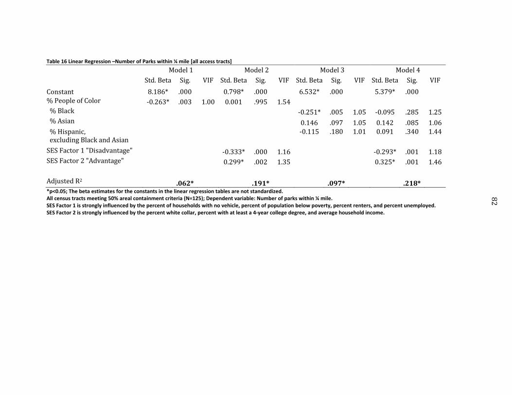
82
Table 16 Linear Regression –Number of Parks within ¼ mile [all access tracts]
Model 1 Model 2 Model 3 Model 4
Std. Beta Sig. VIF Std. Beta Sig. VIF Std. Beta Sig. VIF Std. Beta Sig. VIF Constant 8.186* .000
0.798* .000
6.532* .000
5.379* .000
% People of Color -0.263* .003 1.00 0.001 .995 1.54 % Black
-0.251* .005 1.05 -0.095 .285 1.25
% Asian
0.146 .097 1.05 0.142 .085 1.06 % Hispanic, excluding Black and Asian
-0.115 .180 1.01 0.091 .340 1.44
SES Factor 1 "Disadvantage"
-0.333* .000 1.16
-0.293* .001 1.18 SES Factor 2 "Advantage"
0.299* .002 1.35
0.325* .001 1.46
Adjusted R2
.062*
.191*
.097*
.218* *p<0.05; The beta estimates for the constants in the linear regression tables are not standardized.
All census tracts meeting 50% areal containment criteria (N=125); Dependent variable: Number of parks within ¼ mile. SES Factor 1 is strongly influenced by the percent of households with no vehicle, percent of population below poverty, percent renters, and percent unemployed. SES Factor 2 is strongly influenced by the percent white collar, percent with at least a 4-year college degree, and average household income.
83
Table 17 shows the 71 access tracts (defined by 50% areal containment) that are
within Portland city limits. The percent people of color is negatively correlated with the
number of parks, but once the socio-economic factors are introduced, this significance
disappears. The advantage population is the strongest driver of the number of parks
within ¼ mile of tracts in the City of Portland, and it has a positive and statistically
significant coefficient.

84
Table 17 Linear Regression –Number of Parks within ¼ mile [Portland]
Model 1 Model 2 Model 3 Model 4 Std. Beta
Sig. VIF Std. Beta
Sig. VIF Std. Beta
Sig. VIF Std. Beta
Sig. VIF
Constant 5.361* .000
0.652* .000
5.805* .000
4.252* .000 % People of Color -0.280* .018 1.00 -0.045 .754 1.66
% Black
-0.253 .055 1.26 -0.134 .313 1.41 % Asian
-0.243 .059 1.20 -0.123 .351 1.39
% Hispanic, excluding Black and Asian
-0.070 .573 1.15 0.193 .210 1.88
SES Factor 1 "Disadvantage"
-0.109 .358 1.12
-0.130 .264 1.11 SES Factor 2 "Advantage"
0.361* .011 1.54
0.441* .009 2.17
Adjusted R2
.065*
.128*
.630
.138* *p<0.05; The beta estimates for the constants in the linear regression tables are not standardized.
Only tracts within Portland city limits meeting 50% areal containment criteria (N=71); Dependent variable: Number of parks within ¼ mile. SES Factor 1 is strongly influenced by the percent of households with no vehicle, percent of population below poverty, percent renters, and percent unemployed. SES Factor 2 is strongly influenced by the percent white collar, percent with at least a 4-year college degree, and average household income.
85
For tracts in Beaverton, Gresham, and Hillsboro, Table 18 shows that the only
variable with a significant correlation when the racial/ethnic variables are grouped
together is the advantage socio-economic factor. The advantage socio-economic factor
has a strong positive coefficient of 0.600. When the racial/ethnic groups are broken
down, however, the percent Asian is positively correlated until socio-economic
variables are introduced. In Model 4, once socio-economic factors are added to the
disaggregated racial/ethnic variables, none of the variables have statistically significant
coefficients. The small sample size of 21 tracts may contribute to this.

86
Table 18 Linear Regression –Number of Parks within ¼ mile [major cities]
Model 1 Model 2 Model 3 Model 4 Std. Beta
Sig. VIF Std. Beta
Sig. VIF Std. Beta
Sig. VIF Std. Beta
Sig. VIF
Constant 9.275* .006
2.894 .054
7.585* .017
5.725 .146 % People of Color -0.101 .665 1.00 0.248 .294 1.78
% Black
-0.206 .314 1.00 0.079 .753 1.81 % Asian
0.483* .041 1.21 0.195 .494 2.32
% Hispanic, excluding Black and Asian
-0.105 .637 1.21 0.240 .396 2.26
SES Factor 1 "Disadvantage"
-0.314 .214 2.00
-0.330 .292 2.71 SES Factor 2 "Advantage"
0.600* .005 1.20
0.540 .095 2.75
Adjusted R2
-.042
.410*
.214
.334* *p<0.05; The beta estimates for the constants in the linear regression tables are not standardized.
Only tracts in major cities with population >50,000 meeting 50% areal containment criteria (N=21); Dependent variable: Number of parks within ¼ mile. SES Factor 1 is strongly influenced by the percent of households with no vehicle, percent of population below poverty, percent renters, and percent unemployed. SES Factor 2 is strongly influenced by the percent white collar, percent with at least a 4-year college degree, and average household income.

87
Table 19 shows that in tracts beyond Portland, Beaverton, Gresham, and
Hillsboro, when racial/ethnic variables are grouped together, the disadvantage socio-
economic factor is the only variable that has a significant coefficient. The disadvantage
socio-economic factor is negatively correlated with the number of parks within ¼ mile
of the tract, but the statistical significance of the coefficient disappears when the
racial/ethnic variables are separated. Again, the small sample size of 33 tracts may
contribute to this.
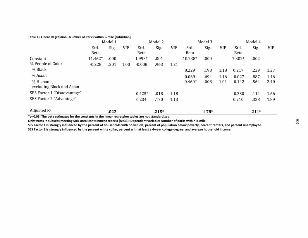
88
Table 19 Linear Regression –Number of Parks within ¼ mile [suburban]
Model 1 Model 2 Model 3 Model 4 Std. Beta
Sig. VIF Std. Beta
Sig. VIF Std. Beta
Sig. VIF Std. Beta
Sig. VIF
Constant 11.462* .000
1.993* .001
10.238* .000
7.302* .002 % People of Color -0.228 .201 1.00 -0.008 .963 1.21
% Black
0.229 .198 1.18 0.217 .229 1.27 % Asian
0.069 .694 1.16 -0.027 .887 1.46
% Hispanic, excluding Black and Asian
-0.460* .008 1.01 -0.142 .564 2.40
SES Factor 1 "Disadvantage"
-0.425* .018 1.18
-0.330 .114 1.66 SES Factor 2 "Advantage"
0.234 .170 1.13
0.210 .338 1.89
Adjusted R2
.022
.215*
.178*
.211* *p<0.05; The beta estimates for the constants in the linear regression tables are not standardized.
Only tracts in suburbs meeting 50% areal containment criteria (N=33); Dependent variable: Number of parks within ¼ mile. SES Factor 1 is strongly influenced by the percent of households with no vehicle, percent of population below poverty, percent renters, and percent unemployed. SES Factor 2 is strongly influenced by the percent white collar, percent with at least a 4-year college degree, and average household income.
89
Parks as Unit of Analysis
When parks are used as the unit of analysis, the demographics refer to the
people living within the ¼-mile access area of the park, whereas the cancer and
respiratory risk variables refer to the risk within the park itself.
Bivariate Correlations: Parks
The correlation results in Table 20 show that the disadvantage factor is strongly
positively correlated with both total cancer and respiratory risks of parks, and the
advantage factor is slightly positively correlated with respiratory risk. The percent
black and percent people of color are positively correlated with the disadvantage factor,
and are also positively correlated with total cancer and respiratory risks of parks. The
percentage of Asian populations is slightly negatively correlated with park cancer risk.
Although there are statistically significant racial/ethnic correlations with cancer and
respiratory risks, the disadvantage factor has the largest statistically significant
correlation coefficients. Additionally, the total cancer and respiratory risks for parks are
strongly correlated with one another. Park area is not significantly correlated with any
of the variables, and thus was omitted from the regression analyses.

90
Table 20 Bivariate Correlations for Demographic and Park Variables
Pearson Correlations % People of Color % Black % Asian
% Hispanic excluding Blacks and Asians
SES Factor 1 "Advantage"
SES Factor 2 "Disadvantage"
Park Area (sq. ft.)
Total Cancer Risk
Total Respiratory Risk
% People of Color 1 .610* .385* .663* -.358* .427* .027 .119* .216* % Black .610* 1 -.051 .090* -.142* .408* .071 .302* .353* % Asian .385* -.051 1 -.115* .215* -.081 -.030 -.132* -.026 % Hispanic excluding Blacks and Asians .663* .090* -.115* 1 -.507* .306* -.004 -.021 .004 SES Factor 1 "Advantage" -.358* -.142* .215* -.507* 1 -.008 -.010 -.067 .140* SES Factor 2 "Disadvantage" .427* .408* -.081 .306* -.008 1 .028 .511* .696* Park Area (sq. ft.) .027 .071 -.030 -.004 -.010 .028 1 .024 .010 Total Cancer Risk .119* .302* -.132* -.021 -.067 .511* .024 1 .764* Total Respiratory Risk .216* .353* -.026 .004 .140* .696* .010 .764* 1
*p<0.05; All public parks (developed with amenities) that are at least 60,000 square feet in size (N=576). SES Factor 1 [unit of analysis: parks] is strongly influenced by the percent with at least a 4-year college degree, percent white collar, and average household income. SES Factor 2 [unit of analysis: parks] is strongly influenced by the percent of households with no vehicle, percent of population below poverty, percent renters, and percent unemployed.

91
Total Cancer Risk of Park
Table 21 shows that the disadvantage socio-economic factor of the people within
the ¼-mile access area of a park is the strongest predictor of the total cancer risk of the
park. The disadvantage socio-economic factor has a positively statistically significant
coefficient, and the advantage socio-economic factor has a negatively statistically
significant coefficient. The percent people of color variable has a positive and
statistically significant bivariate correlation coefficient with park cancer risk, but with
the inclusion of the socio-economic factors, the coefficient becomes negative. This
suggests that the initial racial and ethnic disparities are mostly a function of socio-
economic disparities, and that there is a slight ameliorating effect of race/ethnicity on
the stronger socio-economic predictors of park cancer risk. When the people of color
category is broken down into smaller groups, however, the ameliorating effects seem to
be driven by the Asian and Hispanic populations.

92
Table 21 Linear Regression –Total Park Cancer Risk
Model 1 Model 2 Model 3 Model 4 Std. Beta
Sig. VIF Std. Beta
Sig. VIF Std. Beta
Sig. VIF Std. Beta
Sig. VIF
Constant 64.110* .000
2.134* .000
71.31* .000
79.223* .000 % People of Color 0.119* .004 1.00 -0.176* .000 1.45
% Black
0.301* .000 1.01 0.065 .086 1.25 % Asian
-0.124* .002 1.02 -0.076* .030 1.06
% Hispanic, excluding Black and Asian
-0.062 .121 1.02 -0.308* .000 1.57
SES Factor 1 "Advantage"
-0.125* .001 1.18
-0.193* .000 1.51 SES Factor 2 "Disadvantage"
0.585* .000 1.26
0.572* .000 1.41
Adjusted R2
.012*
.283*
.104*
.336* *p<0.05; The beta estimates for the constants in the linear regression tables are not standardized.
All parks (N=576); Dependent variable: Total cancer risk of park. SES Factor 1 is strongly influenced by the percent with at least a 4-year college degree, percent white collar, and average household income. SES Factor 2 is strongly influenced by the percent of households with no vehicle, percent of population below poverty, percent renters, and percent unemployed.

93
Total Respiratory Risk of Park
Table 22 shows that the disadvantage socio-economic factor of the ¼-mile
access area of a park is the strongest predictor for the total respiratory risk of the park.
The coefficient for the disadvantage socio-economic factor is positively statistically
significant, both in Model 2 with aggregated racial/ethnic variables and in Model 4 with
separated racial/ethnic variables. The advantage socio-economic factor has a smaller
positive and statistically significant coefficient when the percent people of color are
aggregated. The bivariate correlation for the percent people of color is positive and
statistically significant, but with the inclusion of socio-economic factors, the significance
disappears and the coefficient becomes negative, thus suggesting that the initial
positive bivariate correlation is mostly explained by socio-economic status.
Model 4 shows that the percent black has a small positive coefficient when socio-
economic factors are included in the regression, while the percent Hispanic (excluding
black and Asian populations), has a slight ameliorating effect on the correlation
between the disadvantage factor and the park respiratory risk. However, due to its
large coefficient, the disadvantage factor is still the most prominent predictor of park
respiratory risk.
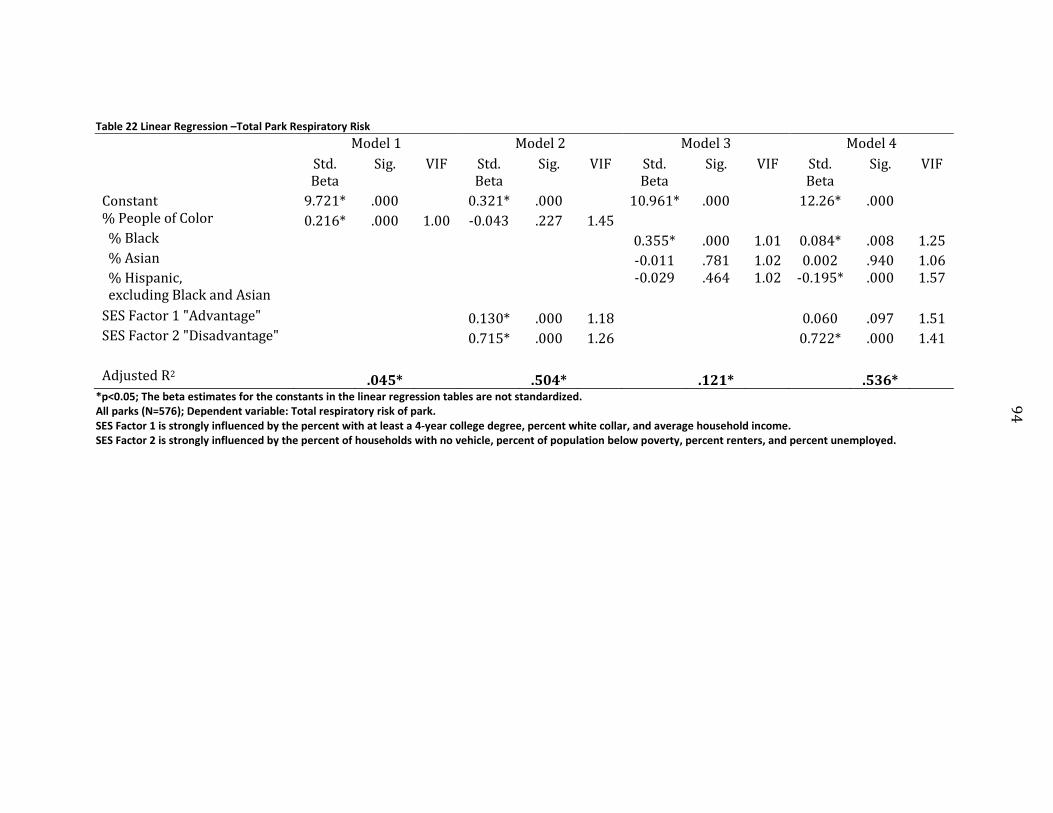
94
Table 22 Linear Regression –Total Park Respiratory Risk
Model 1 Model 2 Model 3 Model 4
Std. Beta
Sig. VIF Std. Beta
Sig. VIF Std. Beta
Sig. VIF Std. Beta
Sig. VIF
Constant 9.721* .000
0.321* .000
10.961* .000
12.26* .000 % People of Color 0.216* .000 1.00 -0.043 .227 1.45
% Black
0.355* .000 1.01 0.084* .008 1.25 % Asian
-0.011 .781 1.02 0.002 .940 1.06
% Hispanic, excluding Black and Asian
-0.029 .464 1.02 -0.195* .000 1.57
SES Factor 1 "Advantage"
0.130* .000 1.18
0.060 .097 1.51 SES Factor 2 "Disadvantage"
0.715* .000 1.26
0.722* .000 1.41
Adjusted R2 .045* .504* .121* .536* *p<0.05; The beta estimates for the constants in the linear regression tables are not standardized. All parks (N=576); Dependent variable: Total respiratory risk of park. SES Factor 1 is strongly influenced by the percent with at least a 4-year college degree, percent white collar, and average household income. SES Factor 2 is strongly influenced by the percent of households with no vehicle, percent of population below poverty, percent renters, and percent unemployed.
95
CHAPTER FIVE - CONCLUSION There has been growing interest in researching the distribution and equity of
environmental amenities such as parks, and this study contributed to this growing
literature by examining parks in the Portland, Oregon region and introducing air quality
as a measure of park quality. Through this study, the main research objectives were
achieved through spatial and statistical analyses. Findings indicate that there are
significant socio-economic influences on park access and air pollution-related cancer
and respiratory risks. Although racial and ethnic disparities regarding park access and
air quality exist in the Portland Metro area, these disparities appear to be driven largely
by socio-economic factors. However, the Portland Metro area has a small proportion of
racial and ethnic minorities compared to other metropolitan areas in the U.S., where
racial/ethnic composition may play a more important role. These results therefore offer
opportunities for further research on park equity and park quality.
The first objective of this study was to examine whether a census tract’s access
to public urban parks was a function of the tract’s racial/ethnic and socio-economic
characteristics, and if these patterns varied depending on whether the tracts were
within the City of Portland, within the major cities of Beaverton, Gresham, and
Hillsboro, or beyond the boundaries of these larger cities and in more suburban areas.
Next, this study explored whether air pollution-related cancer and respiratory risks in a
census tract were a function of the tract’s racial/ethnic and socio-economic
characteristics, and whether these patterns varied depending on the tract geography.
Another objective was to examine whether the number of public urban parks within a

96
quarter-mile of a tract was a function of the racial/ethnic and socio-economic
demographics of a tract, and whether this varied based on the location of the tract. This
study also analyzed whether air pollution-related cancer and respiratory risks within a
public urban park were a function of the racial/ethnic and socio-economic
characteristics of residents within a ¼ mile of the park. Finally, the study weighed the
relative importance of race/ethnicity versus socio-economic status in affecting these
park access and air quality outcomes.
Summary of Findings
Overall, the regression analyses in this study demonstrated that socio-economic
factors were the strongest predictors of park access and air pollution-related cancer
and respiratory risks. Specifically, when examining the cancer and respiratory risks of
census tracts and parks, the disadvantage socio-economic factor emerged with the
largest statistically significant coefficients. This disadvantage factor was most strongly
influenced by the percent of households with no vehicle, percent of population below
poverty, percent renters, and percent unemployed, and as these percentages within the
tract or ¼-mile access area increased, the tract or park cancer and respiratory risks
increased as well. For analyzing the number of parks within ¼ mile of tracts, however,
the advantage and disadvantage socio-economic factors had more equal influences. The
greater the percent with at least a 4-year college degree, percent white collar, and
average household income, as well as the lower the percent of households with no
vehicle, percent of population below poverty, percent renters, and percent unemployed,
the greater the number of parks within ¼ mile of a tract. Thus, the level of disadvantage
97
in the population specifically drives cancer and respiratory risks, while socio-economic
factors in general influence the number of parks within ¼ mile of a tract.
When separating the tracts by tract geography, tracts within the City of Portland
displayed similar trends to those of all tracts in the Metro boundary. However, the
major cities of Beaverton, Gresham, and Hillsboro did not display any statistically
significant demographic predictors for park access or air pollution-related cancer or
respiratory risks. This may be partially explained by the smaller number of tracts
within these major cities, as well as by underlying differences in demographics across
the three cities, despite their similar population sizes within the Metro boundary. The
suburban tracts beyond these major cities displayed trends that were similar to those of
the overall region for air pollution-related cancer and respiratory risks, but did not
have statistically significant demographic predictors for the number of parks within ¼
mile of a tract. In determining whether a tract was an access tract based on 50% areal
containment, suburban tracts with the percentage of blacks exceeding the median
percentage were negative predictors for the tract being considered an access tract.
Thus, to summarize the main findings of this study, socio-economic factors were
the strongest predictor for park access and air pollution-related cancer and respiratory
risks. Tracts within the City of Portland displayed similar results to those of the entire
metropolitan region, while tracts in major cities did not demonstrate any significant
demographic predictors of park access or air pollution-related health risks. Suburban
tracts shared similar results with the entire metropolitan region for cancer and
respiratory risks, but did not display significant demographic predictors for the number
of parks within ¼ mile of a tract. Overall, racial/ethnic disparities in park access and air
98
quality exist, but these appear to be related to racial and ethnic disparities in socio-
economic advantage, reflecting the effect of a long history of racial discrimination and
housing segregation in the U.S.
Significance of Findings
These conclusions are important, because they bring together the studies of
disparities in the distribution of both environmental amenities and environmental
burdens. Census tracts with high levels of disadvantaged populations tend to have
higher cancer and respiratory risks and less access to parks. Thus, the distribution of
parks and park air quality exacerbates existing inequalities within the Portland region.
By introducing air quality as a measure of park quality, this study also highlights
significant demographic differences among communities that surround parks with
differing levels of cancer and respiratory risks. Existing literature has demonstrated
that environmental burdens such as pollution are inequitably distributed (Chavis and
Lee 1987, Bullard, et al. 2007, Ringquist 2005), and the results from this study further
support this. Particularly with the public health argument for parks to serve as places
for physical activity, the air quality of parks should be further examined (Roemmich, et
al. 2006, Cohen, et al. 2007, Lopez and Hynes 2006).
While some existing environmental justice studies have found race to be a
significant predictor of environmental burdens and access to environmental amenities,
this study concluded that socio-economic status is the primary predictor of air quality
and park access in Portland (Ringquist 2005, Wolch, Wilson and Fehrenbach 2005,
Boone, et al. 2009). Despite socio-economic variables having a larger influence than
racial variables in determining park access and air quality, the bivariate correlations

99
between the racial/ethnic variables and these measures of park access and air quality
indicate that racial/ethnic minorities still experience higher air pollution levels and
access to fewer parks than their white, non-Hispanic counterparts. Thus, although race
may help ameliorate the strong correlation between socio-economic status and air
quality and park access in some cases, people of color in Portland still have high levels
of disadvantage that affect their cancer and respiratory risks and park access.
Given the disparities in race/ethnicity in socio-economic status, as well as the
inequitable distribution of parks and air quality, Portland displays effects of indirect
institutionalized discrimination (Feagin and Feagin 1986). Especially with the potential
benefits that parks can bring to a neighborhood, the lower park access in communities
already disadvantaged by historical discrimination further widens the gap between the
advantaged and disadvantaged populations in Portland.
This study therefore offers insight on equity issues in a park-rich and
progressive region such as Portland. In a city that prides itself on sustainability and
environmental issues, this study suggests that the distribution of environmental
amenities and burdens should be integrated into future planning efforts in the region.
Future Research
This study demonstrated that disparities are present in park access and air
quality in Portland, and thus provides opportunities to continue examining air quality
as a measure of park quality in other cities. Other measures of park quality used in
existing research, such as park congestion and park maintenance, can be used in
combination with air quality to more fully assess park equity. Furthermore,
measurements of direct park usage may also enhance future research.

100
Additionally, measures of tract geography can be modified and applied to other
regions. In this study, the separation of tracts by location helped to elucidate some
trends within the metropolitan region, and further examination of spatial scales may be
valuable in environmental justice research. Replicating this study in other metropolitan
areas with different racial/ethnic compositions and histories, different patterns of
industrial pollution, and different park distributions would also be valuable. Studies on
the equity and distribution of environmental amenities should also expand to include
areas similar to Portland, where issues of socio-economic and racial/ethnic
environmental disparities are often overshadowed by prominent displays of innovative
environmental practices in wealthier neighborhoods.
Finally, additional environmental justice studies that integrate both
environmental amenities and environmental burdens are needed. Environmental
amenities and burdens are often tightly linked, as the creation of an environmental
amenity may inevitably result in an externality that negatively impacts another
community. For example, a community that successfully preserves green space by
preventing an industrial facility from being sited in its neighborhood may merely cause
the facility to be built in another community (Schelly and Stretesky 2009). Thus, in
order to fully assess environmental justice, access to environmental amenities and
environmental burdens should be jointly examined.
101
LITERATURE CITED Barbosa, O., et al. "Who benefits from access to green space? A case study from Sheffield,
UK." Landscape and Urban Planning 83 (2007): 187-195. Bedimo-Rung, A.L., A.J. Mowen, and D.A. Cohen. "The significance of parks to physical
activity and public health." American Journal of Preventative Medicine, 2005: 159-166.
Benedict, M.A., and E.T. McMahon. "Green Infrastructure: Smart Conservation for the 21st Century." In Green Infrastructure/Urban Parks: Selected References, edited by The Conservation Fund. Urban Land Institute, 2002.
Bolitzer, B., and N.R. Netusil. "The impact of open spaces on property values in Portland, Oregon." Journal of Environmental Management 59 (2000): 185-193.
Boone, C.G., G.L. Buckley, J.M. Grove, and C. Sister. "Parks and people: An environmental justice inquiry in Baltimore, Maryland." Annals of the Association of American Geographers 99, no. 4 (2009): 767-787.
Branis, M., J. Safranek, and A. Hytychova. "Exposure of children to airborne particulate matter of different fractions during indoor physical education at school." Building and Environment 44 (2009): 1246-1252.
Bullard, R.D., P. Mohai, R. Saha, and B Wright. Toxic Waste and Race at Twenty: Grassroots Struggles to Dismantle Environmental Racism in the United States. Cleveland, OH: United Church of Christ, 2007.
Chavis, B.F., and C. Lee. Toxic Waste and Race in the United States. New York: United Church of Christ, 1987.
Cohen, D.A., T.L. McKenzie, A. Sehgal, S. Williamson, D. Golinelli, and N Lurie. "Contribution of public parks to physical activity." American Journal of Public Health 97, no. 3 (2007): 509-514.
Cole, L.W., and S.R Foster. From the Ground Up: Environmental Racism and the Rise of the Environmental Justice Movement. New York: New York University Press, 2001.
Egan, N., and P. Nakazawa. "After Olmsted." In Green Infrastructure/Urban Parks: Selected References, edited by Urban Land Institute. 2007.
Environmental Protection Agency. National Air Toxics Assessments. 2010. http://www.epa.gov/ttn/atw/natamain/. (accessed August 17, 2011).
Feagin, J., and C.B Feagin. Discrimination American Style: Institutional Racism and Sexism. 2nd. Malabar, FL: Krieger Publishing Co., 1986.
Gandy, M. Concrete and Clay: Reworking Nature in New York City. Cambridge, MA: MIT Press, 2003.
García, R., and A. White. "Healthy parks, schools, and communities: Mapping green access and equity for the Los Angeles region." The City Project. 2006. http://www.cityprojectca.org/ourwork/mappinggreenaccess/index.html (accessed June 27, 2010).
Garry, V.F., M.E. Harkins, L.L. Erickson, L.K. Long-Simpson, S.E. Holland, and B.L. Burroughs. "Birth defects, season of conception, and sex of children born to pesticide applicators living in the Red River Valley of Minnesota, USA." Environmental Health Perspectives 110 (2002): 441-449.
102
Geschwind, S.A., et al. "Risk of congenital malformations associated with proximity to hazardous waste sites." American Journal of Epidemiology 135, no. 11 (1992): 1197-1206.
Giles-Corti, B., et al. "Increasing walking: How important is distance to, attractiveness, and size of public open space?" American Journal of Preventative Medicine 28 (2005): 169-176.
Gordon-Larsen, P., M.C. Nelson, P. Page, and B.M. Popkin. "Inequality in the built environment underlies key health disparities in physical activity and obesity." Pediatrics 117, no. 2 (2006): 417-424.
Hall, M., and B. Lee. "How diverse are US Suburbs?" Urban Studies 47, no. 1 (2009): 3-28. James, P., et al. "Towards an integrated understanding of green space in the European
built environment." Urban Forestry & Urban Greening 8 (2009): 65-75. Johnston, M., and L.D. Shimada. "Urban forestry in a multicultural society." Journal of
Arboriculture 30, no. 3 (2004): 185-192. Kaczynski, A.T., L.R. Potwarka, and E. Saelens. "Association of park size, distance, and
features with physical activity in neighborhood parks." American Journal of Public Health 98, no. 8 (2008): 1451-1456.
Kipke, M.D., et al. "Food and park environments: Neighborhood-level risks for childhood obesity in east Los Angeles." Journal of Adolescent Health 40 (2007): 325-333.
Kuehn, R. "A taxonomy of environmental justice issues." Environmental Law Reporter 30 (2000): 10681-10703.
Kumanyika, S., and S. Grier. "Targeting interventions for ethnic minority and low-income populations." The Future of Children 16, no. 1 (2006): 187-207.
Portland: Question for the Livable City. Directed by T. Lay. Produced by Northern Light Productions. 2009.
Lee, S. "Analyzing intra-metropolitan poverty differentiation: causes and consequences of poverty expansion to suburbs in the metropolitan Atlanta region." The Annals of Regional Science 46, no. 1 (2011): 37-57.
Lindsey, G., M. Maraj, and S. Kuan. "Access, equity, and urban greenways: An exploratory investigation." Professional Geographer 53 (2001): 332-346.
Liu, B., and J.M. Vanderleeuw. "Economic Development Priorities and Central-City and Suburb Differences." American Politics Research, 2004: 698-721.
Lockwood, C. "Bagby-to-Sabine: A New Beginning." In Green Infrastructure/Urban Parks: Selected References. Urban Land Institute, 2007.
Lopez, R.P., and H.P. Hynes. "Obesity, physical activity, and the urban environment: Public health research needs." Environmental Health 5 (2006): 25-35.
Louv, R. Last Child in the Woods. Chapel Hill, NC: Algonquin Books, 2005. Maantay, J. "Asthma and air pollution in the Bronx: Methodological and data
considerations in using GIS for environmental justice and health research." Health & Place 13 (2007): 32-56.
Massey, D.S. "Segregation and stratification: A biosocial perspective." Du Bois Review 1, no. 1 (2004): 7-25.
Mayer, H., and J. Provo. "The Portland Edge in Context." In The Portland Edge, edited by C. Ozawa, 9-34. Washington, DC: Island Press, 2004.

103
Metro. "Metropolitan Greenspaces Master Plan." Metro. July 1992. http://library.oregonmetro.gov/files//doc10_794_metropolitan_greenspaces_master_plan.pdf (accessed March 19, 2012).
—. RLIS Metadata. 2010. http://rlismetadata.oregonmetro.gov (accessed August 17, 2011).
—. Welcome to Metro. 2012. http://www.oregonmetro.gov/ (accessed August 27, 2011).
Mohai, P., and B. Bryant. "Environmental racism: Reviewing the evidence." In Race and Incidence of Environmental Hazards: A Time for Discourse, edited by B. Bryant and P. Mohai, 163-176. Boulder, CO: Westview Press, 1992.
Mohai, P., and R. Saha. "Reassessing Racial and Socioeconomic Disparities in Environmental Justice Research." Demography 43, no. 2 (2006): 383-399.
Mohai, P., D. Pellow, and J.T. Roberts. "Environmental Justice." Annual Review of Environment & Resources 34 (2009): 16.1-16.26.
Morello-Frosch, R., and B.M. Jesdale. "Separate and Unequal: Residential Segregation and Estimated Cancer Risks Associated with Ambient Air Toxics in U.S. Metropolitan Areas." Environmental Health Perspectives 114, no. 3 (2006): 386-393.
Morrill, A.C., and C.D. Chinn. "The obesity epidemic in the United States." Journal of Public Health Policy 25, no. 3/4 (2004): 353-366.
Mossop, E. "Landscapes of infrastructure." In The Landscape Urbanism Reader, edited by Charles Waldheim. New York: Princeton Architectural Press, 2006.
National People of Color Environmental Leadership Summit. "Principles of Environmental Justice." 1991.
Nelson, A.C., and T. Moore. "The case of Portland, Oregon, the USA's largest urban growth boundary." Land Use Policy, October 1993: 293-302.
New Yorkers for Parks. "Parks for All New Yorkers: Immigrants, Culture, and NYC Parks." New Yorkers for Parks. 2009. http://www.ny4p.org (accessed June 27, 2010).
Oregon Department of Education. "Oregon Racial Laws and Events 1844-1859." n.d. http://www.ode.state.or.us/opportunities/grants/saelp/orraciallaws.pdf (accessed 04 04, 2012).
Pastor, M., J. Sadd, and J. Hipp. "Which came first? Toxic facilities, minority move-in, and environmental justice." Journal of Urban Affairs 23 (2001): 1-21.
Pastor, M., R. Morello-Frosch, and J.L. Sadd. "Breathless: Schools, air toxics, and environmental justice in California." The Policy Studies Journal 34, no. 3 (2006): 337-362.
Potwarka, L.R., and A.T. Kaczynski. "Places to play: Association of park space and facilities with healthy weight status among children." J. Community Health 33 (2008): 344-350.
Ringquist, E.J. "Assessing evidence of environmental inequities: A meta-analysis." Journal of Policy Analysis and Management 24, no. 2 (2005): 223-247.
Roemmich, J.N,, L.H. Epstein, S. Raja, L. Yin, J. Robinson, and D. Winiewicz. "Association of access to parks and recreational facilities with the physical activity of young children." Preventative Medicine 43 (2006): 437-441.
104
Russ, T.H. Site Planning and Design Handbook. 2nd Edition. New York: McGraw-Hill, 2009.
Sallis, J.F., and K. Glanz. "The role of built environments in physical activity, eating, and obesity in childhood." Future of Children 16, no. 1 (2006): 89-108.
Schelly, D., and P.B. Stretesky. "An Analysis of the "Path of Least Resistance" Argument in Three Environmental Justice Success Cases." Society and Natural Resources 22 (2009): 369-380.
Seltzer, E. "It's not an experiment: Regional planning at Metro, 1990 to the present." In The Portland Edge, by C. Ozawa, 35-60. Washington, DC: Island Press, 2004.
The Brookings Institution. "Portland in Focus: A Profile from Census 2000." Brookings. November 2003. http://www.brookings.edu/reports/2003/11_livingcities_portland.aspx (accessed April 04, 2012).
The City Project. The City Project. 2010. http://www.cityprojectca.org (accessed June 27, 2010).
U.S. Census Bureau. American FactFinder: Decennial Census. 2000. http://factfinder.census.gov (accessed December 14, 2011).
Williams, D.R., and C. Collins. "Racial residential segregation: A fundamental cause of racial disparities in health." Public Health Reports 116, no. 5 (2001): 404-417.
Wolch, J., J.P. Wilson, and J. Fehrenbach. "Parks and park funding in Los Angeles: An equity-mapping analysis." Urban Geography 26 (2005): 4-35.

105
APPENDIX A: REGIONAL LAND INFORMATION SYSTEM (RLIS) DATA Appendix A - Table 1 RLIS Data Layers
RLIS Data Layer Description 2000 Census Tracts Boundaries of Census tracts from the 2000 Census Metro Boundary The political boundary for the regional government of Metro City Limits City boundaries for incorporated cities Parks and Greenspaces Public and private parks and green spaces
Appendix A - Table 2 RLIS Park and Ownership Categories RLIS Park Categories Categories Used in This Study Developed park site with amenities ● Open space or natural area without amenities Common area of a subdivision or condominium complex Cemetery Golf course School grounds or school park Pool Tennis courts Fairgrounds, fields or stadium use Community Center Trail or path Community Garden RLIS Usage Categories (Park Ownership) Privately-owned open space or common area
Publicly-owned parcels ●

106
APPENDIX B: 2000 CENSUS DATA – SUMMARY FILE 3 Appendix B - Table 1 Race Variables
Categories Used in This Study
Census Categories (Summary Table P6) Black Asian White alone Black or African American alone ● American Indian and Alaska Native alone Asian alone ● Native Hawaiian and Other Pacific Islander alone Some other race alone Two or more races
Appendix B - Table 2 Ethnicity Variables
Categories Used in This Study
Census Categories (Summary Table P7) White, non-
Hispanic
Hispanic, excluding Black and
Asian People of
Color Not Hispanic or Latino: White alone ● Black or African American alone ● American Indian and Alaska Native alone ● Asian alone ● Native Hawaiian and Other Pacific Islander alone ● Some other race alone ● Two or more races ● Hispanic or Latino: White alone ● ● Black or African American alone ● American Indian and Alaska Native alone ● ● Asian alone ● Native Hawaiian and Other Pacific Islander alone ● ● Some other race alone ● ● Two or more races ● ●
Appendix B - Table 3 Dummy Variable Creation for Race/Ethnicity
Dummy Variable Assignment
Racial/Ethnic Variable
Median Percentage in
Tract 0 1
People of Color 0.191367 ≤0.191367 >0.191367 White, non-Hispanic 0.808600 ≤0.808600 >0.808600 Black 0.014096 ≤0.014096 >0.014096 Asian 0.045400 ≤0.045400 >0.045400 Hispanic, excluding Black and Asian 0.055200 ≤0.055200 >0.055200
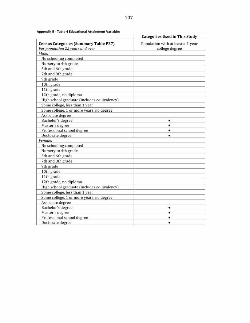
107
Appendix B - Table 4 Educational Attainment Variables
Categories Used in This Study
Census Categories (Summary Table P37) For population 25 years and over
Population with at least a 4-year college degree
Male: No schooling completed
Nursery to 4th grade 5th and 6th grade 7th and 8th grade 9th grade 10th grade 11th grade 12th grade, no diploma High school graduate (includes equivalency) Some college, less than 1 year Some college, 1 or more years, no degree Associate degree Bachelor's degree ● Master's degree ● Professional school degree ● Doctorate degree ● Female: No schooling completed Nursery to 4th grade 5th and 6th grade 7th and 8th grade 9th grade 10th grade 11th grade 12th grade, no diploma High school graduate (includes equivalency) Some college, less than 1 year Some college, 1 or more years, no degree Associate degree Bachelor's degree ● Master's degree ● Professional school degree ● Doctorate degree ●

108
Appendix B - Table 5 Occupational Variables
Categories Used in This Study
Census Categories (Summary Table P50) For population 16 years and over White Collar Workers Male: Management, professional, and related occupations ● Service occupations Sales and office occupations Farming, fishing, and forestry occupations Construction, extraction, and maintenance occupations Production, transportation, and material moving occupations Female: Management, professional, and related occupations ● Service occupations Sales and office occupations Farming, fishing, and forestry occupations Construction, extraction, and maintenance occupations Production, transportation, and material moving occupations
Appendix B - Table 6 Single Female-Headed Household Variable
Categories Used in This Study
Census Categories (Summary Table P17) For all families Single Female-Headed Households Married-couple family: With related children under 18 years No related children under 18 years Other family: Male householder, no wife present: With related children under 18 years No related children under 18 years Female householder, no husband present: With related children under 18 years ● No related children under 18 years
Appendix B - Table 7 Unemployment Variables
Categories Used in This Study
Census Categories (Summary Table P43) For population 16 years and over Unemployed Male: In labor force: In Armed Forces Civilian: Employed Unemployed ● Not in labor force Female: In labor force: In Armed Forces Civilian: Employed Unemployed ● Not in labor force

109
Appendix B - Table 8 Citizenship Variables
Categories Used in This Study
Census Categories (Summary Table P43) Unemployed Native: Born in state of residence Born in other state in the United States Born outside the United States Foreign born: Naturalized citizen Not a citizen ●