Phil. Trans. R. Soc. A (2011) 369, 1–30doi:10.1098/rsta.2011.0160

Environmental prediction, risk assessment andextreme events: adaptation strategies for the

developing worldBY PETER J. WEBSTER1,* AND JUN JIAN2

1School of Earth and Atmospheric Sciences, Georgia Institute of Technology,Atlanta, GA, USA

2Navigation College, Dalian Maritime University, Dalian 116026,People’s Republic of China

The uncertainty associated with predicting extreme weather events has seriousimplications for the developing world, owing to the greater societal vulnerability to suchevents. Continual exposure to unanticipated extreme events is a contributing factor forthe descent into perpetual and structural rural poverty. We provide two examples of howprobabilistic environmental prediction of extreme weather events can support dynamicadaptation. In the current climate era, we describe how short-term flood forecasts havebeen developed and implemented in Bangladesh. Forecasts of impending floods withhorizons of 10 days are used to change agricultural practices and planning, store food andhousehold items and evacuate those in peril. For the first time in Bangladesh, floods wereanticipated in 2007 and 2008, with broad actions taking place in advance of the floods,grossing agricultural and household savings measured in units of annual income. We arguethat probabilistic environmental forecasts disseminated to an informed user communitycan reduce poverty caused by exposure to unanticipated extreme events. Second, it isalso realized that not all decisions in the future can be made at the village level andthat grand plans for water resource management require extensive planning and funding.Based on imperfect models and scenarios of economic and population growth, we furthersuggest that flood frequency and intensity will increase in the Ganges, Brahmaputra andYangtze catchments as greenhouse-gas concentrations increase. However, irrespective ofthe climate-change scenario chosen, the availability of fresh water in the latter half of thetwenty-first century seems to be dominated by population increases that far outweighclimate-change effects. Paradoxically, fresh water availability may become more criticalif there is no climate change.

Keywords: uncertainty; climate; adaption

1. Introduction

One of the great challenges of weather and climate science is estimating theprobability of the occurrence, severity and duration of an extreme event, as well asits severity and duration, and when and where the event will take place. Tropical*Author for correspondence (pjw@eas.gatech.edu).

One contribution of 15 to a Discussion Meeting Issue ‘Handling uncertainty in science’.

This journal is © 2011 The Royal Society1

2 P. J. Webster and J. Jian

G

0–55–2525–5050–100

people per km2100–250250–400

BY

Figure 1. The Himalayas and the Tibetan Plateau are the sources for a complex of major riversassociated with thriving agricultural societies, colour coded by population density. The Ganges(G), the Brahmaputra (B) and the Yangtze (Y) are outlined. These deltas are currently the hometo 14% of the human population on the planet. Three river staging stations, the Hardinge Bridge onthe Ganges, Bahadurabad on the Brahmaputra and Datong on the Yangtze are shown as blue dots.

cyclones, prolonged droughts and flooding are extreme environmental eventsthat can invoke severe economic cost, societal disruption, death and destruction.Advanced warning of an extreme event allows for preparation, possible evacuationand the marshalling of emergency systems and personnel to help in the mitigationof its effects.

This paper addresses the application of ensemble weather and climate modelsimulations to aid the less-developed world to adapt to extreme events andclimate change. In the more-developed world, solid infrastructure and economicrobustness allows for the impact of extreme events to be absorbed by the largernational community through hedging, insurance and/or government support. Inthe United States, for example, regions impacted by floods and hurricanes maybe declared as ‘federal disaster regions’, allowing communities to receive rapidfiscal and personnel aid from government and non-government organizations.Cuaresma et al. [1] even argue that a natural disaster in a developed countrymay provide ‘constructive destruction’ where destroyed infrastructure is replacedby more modern artefacts. However, the developing world has generally far feweroptions [2].

Developing countries in South and East Asia (figure 1) are especially vulnerableto extreme weather and climate events, particularly from floods and tropicalcyclones. However, these nations often lack the fiscal resilience and the

Phil. Trans. R. Soc. A (2011)

Prediction, risk, floods, adaption 3

infrastructure to minimize the impacts of extreme events or to be able to recoverfrom them quickly. Devastating floods or a land-falling tropical cyclone may leadto nation-wide fiscal problems and perhaps accelerants of political unrest [3,4].At the community or village level, the impact is even more severe, forcing manyinto transient poverty when income is temporally less than expenses [5]. Exposureto multiple extreme events can transform temporary poverty into structural andendemic poverty and possibly perpetual intergenerational poverty [5].

Environmental catastrophes produce great and sudden harm and occursufficiently irregularly to make preparations difficult. Catastrophes are differentfrom static and perpetual natural hazards such as the arsenic contamination ofartesian water in Bangladesh and in other Asian countries [6,7]. For these hazards,relatively inexpensive technological solutions are available for groundwatercontamination through the distribution of effective filters (e.g. [8]), requiringmerely the will, training and finances. Engineering solutions to counter floodand tropical cyclone surges, on the other hand, are expensive and often evenbeyond the resources of developed countries. However, if the catastrophic eventcan be forecast then, mitigatory actions can be undertaken to reduce its impact.The longer the lead time of a warning of an impending event and the greaterthe specificity of the forecasts, the greater the chances are of protecting lives,property and resources.

Consider the short-term impacts of extreme events in Bangladesh, located atthe apex of the Bay of Bengal on the delta of the Ganges and the Brahmaputrarivers (figure 1). Bangladesh had a population of about 160 million in 2009 withinan area the size of England [9]. Although great strides have been made in reducingbirth rate, it still stands at 2.5 per cent per year, providing a population doublingtime of about 30–40 years. The location of Bangladesh makes it especiallysusceptible to tropical cyclones and flooding. During the summer monsoon period(June–September), slow-rise floods inundate large parts of India and Bangladesh,affecting over 40 million people each year. In India, an average of 60 × 103 km2 ofland (approximately equivalent to the size of Texas, Ireland or Norway) is floodedannually [10,11], with an additional 20 × 103 km2 in Bangladesh. In each country,the consequences of flooding are devastating and endlessly impoverishing. Eachyear before planting, farmers borrow against potential income to be earned atthe end of a successful season. These loans are used for future agricultural inputs(seed, fertilizer, pesticides, equipment, stock). The loss of a crop or stock animalsduring a flood period typically puts a farmer in debt for many years, by whichtime the cycle of flooding is repeated, condemning the next generation to lives ofpoverty in repaying debt. Floods are not restricted to the summer. During spring,short-lived deluges associated with pre-monsoon thunderstorms and mesoscaleconvective events create flash floods that destroy large areas of winter rice [12].

In 1987, 1988 and 1998, extensive flooding occurred throughout Bangladeshwhen both the Ganges and the Brahmaputra crested simultaneously well abovetheir flood levels. It is estimated that in 1988 and 1989, 3000 people lost theirlives, homes of millions were destroyed and over 200 000 cattle drowned. In 1998,over two-thirds of the country was submerged for 3 months, and an estimated1000 people drowned, with millions left homeless [13,14]. In 2004, 2007 and 2008,shorter term flooding lasting 10 days or so occurred along the Brahmaputra.Although not as devastating as the earlier prolonged floods, these widespreadinundations impacted millions of people. Societal vulnerability had increased

Phil. Trans. R. Soc. A (2011)

4 P. J. Webster and J. Jian

during the previous decade owing to the rapidly growing population (e.g. [15])that has forced many people to farm the fertile chars (river islands) prone tochronic flooding, and even disappearance, during a flood.

The location of Bangladesh at the head of the Bay of Bengal also makes itespecially susceptible to land-falling tropical cyclones during the boreal springand autumn. Most loss of life and damage is associated with wind-driven stormsurges that often inundate areas of tens of kilometres of the flat delta. In fact,the Bay of Bengal is home to 7 of the 10 most deadly tropical cyclones inrecorded history.

This paper provides two examples from the South Asia region wherebyanticipation of extreme events through probabilistic weather and climate forecastscould enable a user group to minimize their adverse impacts. Two different timescales are considered: the time scale of days to weeks, with regard to a specificimpending extreme event; and the time scale of decades, with regard to thechanging statistics of extreme events that may attend climate change. The firsttask addresses what can be done with present environmental weather and climatemodels to allow adaptation and minimization of loss. We use, as an example, theimmediate problem of providing forecasts of river delta flooding in river deltason time scales that allow agricultural adaptation, minimization of property lossand evacuation. We also discuss the manner in which these forecasts can becommunicated directly to those that will benefit most from advanced warning. Weprovide examples in §3 of the economic benefit of accurate and timely short-term(1–10 days) forecasts at the community level. In a region anticipating long-termclimate change and a possibility of increased frequency of extreme events, long-term planning is required, which may require the building of dams, dykes andriver diversions. With a background of rapidly growing population, there is theimportant issue of ensuring food security, fresh water availability and energyproduction. An example is provided using climate models in a range of economicand demographic scenarios of the twenty-first century to assess risk of futurefloods and fresh water availability in South and East Asia.

2. Determining the risk of an extreme event

In order to adapt to the impacts of an extreme weather event through theadoption of some strategy (e.g. choosing a drought-resistant crop, plant or harvestearly or later) or reduce its impacts (e.g. change water resource managementstrategies), it is necessary to determine the likelihood of an extreme eventoccurring in a particular location and time. This can be accomplished fromhistorical data, experience and intuition, and quantitative probabilistic weatherand climate forecasts.

Managing weather risk may be thought of as a game of roulette [16,17] inwhich an event is forecast by the ball falling on either a red or black slot. Withno information, there is an equal likelihood of the ball falling into a red or blackslot (ignoring the double zero slot). If it is known that slow-rise floods only occurin a particular part of the river delta once every 5 years, our environmentalroulette wheel may have five times as many black slots (no flood) than red slots(flood). Each year, the wheel is spun, but each year, the result is independent ofthe previous spin or last year’s result. What we would like to do at the beginning

Phil. Trans. R. Soc. A (2011)

Prediction, risk, floods, adaption 5

of each monsoon season is to use information that would change the proportion ofred and black slots for a particular forthcoming period of time, month or season.The goal is to develop information that will bias the number of coloured slots byusing quantitative probabilistic weather and climate-prediction models, so thatuser communities can place ‘informed bets’ on how to manage their resources. Byattempting to determine the future state of the environment, weather and climatemodels provide information that reduce or increase the odds of an extreme eventoccurring. A model simulation commences at some prescribed time with initialdata that describes to the best of our knowledge the state of the atmosphere,ocean, land surface, etc. But there are two problems associated with numericalweather and climate models.

— Model error. All models possess bias. Using the roulette analogy, onemodel may have the propensity to tilt towards more red slots than black,while another model tilts towards more black slots. Model errors arisefrom formulations that attempt to replicate continuous laws of physicsand thermodynamics in point-wise space, different methods of numericalsolutions, and the manner in which processes occurring on scales smallerthan the finite elements of the model are taken into account.

— Uncertainty in initial conditions. A model must be provided with a setof initial conditions that define the state of the global weather or climatesystem at a given time. The state of the climate system is not knownexactly, and small differences between the real state (which is never known)and the approximate state may lead to large nonlinear error growth intime [18,19].

Clearly, the prediction tools that we possess are imperfect because of both modelbias and sensitivity to uncertainties in initial conditions. The most importantquestion becomes: with the uncertainty associated with imperfect models andpoorly defined initial conditions, can a credible forecast be provided and used toreduce vulnerability and risk?

There are a number of techniques that can be used to characterize modelforecast uncertainty and minimize error in a prediction. First, one can use thepredictions of many models with the same sets of initial conditions to produce amulti-model mean. The assumption is that each model has different biases thatare randomly distributed among the models that ‘average out’ in producing themulti-model mean. This is a relatively weak assumption as some errors, especiallythose associated with the parameterization of sub-grid processes, are common tomany models.

Sensitivity to initial condition error and the resulting nonlinear error growthmay be assessed through making incremental changes to the model initialconditions (e.g. [20]) or to the parameters that define the representation ofsub-grid processes, and running the model many times with their perturbedinitial conditions. For example, the European Centre for Medium Range WeatherForecasts (ECMWF) runs 51 ensemble members during each forecast cycle[21]. These forecasts, run twice per day out to 15 days produce a swath offorecasts that tend to diverge with time. While the mean of all of the ensemblemembers provides some statistical information about the evolution of weather

Phil. Trans. R. Soc. A (2011)

6 P. J. Webster and J. Jian

month

temperature anomaly (K) –0.5

prob

abili

ty (

%)

100

80

60

40

20

0

tem

pera

ture

ano

mal

y (K

)

+2

+1

0

–1

–2J F M A M J J A S O N

(a)

(b)

J AS O N

observed

ensemble mean

ensemble members

J

JJ

A

S O N

DSSTcrit

+2.5+2.0+1.5+1.0+0.50

Figure 2. Example of an ensemble forecast from the ECMWF system 3 coupled ocean–atmosphereclimate model [22] predicting the evolution of the mid-eastern equatorial Pacific Ocean sea-surfacetemperature (SST) anomaly (deviation from climatology). Positive (negative) anomalies indicatethe advent of an El Niño (La Niña). (a) Evolution of the 41 ensemble members initialized in April2009. The spread of the ensembles allows the determination of the probability of an anomaly ofa particular magnitude. Vertical lines indicate the spread of the ensembles for June (J), July (J),. . . November (N). (b) Probability density functions (pdfs) of the SST anomaly at the end of eachforecast month. With increasing lag, the pdf moves progressively to warmer temperatures. Theprobability of the SST exceeding some critical value (DSSTcrit) is discussed in the text.

or climate, it is the divergence of the ensemble members that provides themost important information about the predictability of the future state of theenvironment.

Model bias and ensemble spread tell us what we do and do not know about thestate and future of the system we are trying to predict. But given that uncertainty,the ensemble spread of the weather or climate forecasts can also be used toprovide an assessment of the probability of an event of a particular magnitudeoccurring at some time in the future. Figure 2 presents an example of an ensembleforecast from the ECMWF system 3 coupled ocean–atmosphere climate model[22] initialized in April 2009. It shows predictions of the mid-eastern equatorialPacific Ocean sea-surface temperature (SST) anomaly or the deviation of the SSTfrom climatology. The SST anomaly in this area of the equatorial Pacific Ocean

Phil. Trans. R. Soc. A (2011)

Prediction, risk, floods, adaption 7

(160 E–150 W, 5 N–5 S, known as the Niño-4 region) is a measure of whetheror not there will be an El Niño or La Niña or neutral conditions. The ensemblemembers provide an estimate, at some time in the future, of the probability ofthe occurrence of an event of a particular magnitude (figure 2a). The individualensemble simulations can be used to form a probability density function (pdf)of the regional ocean temperature (figure 2b). Each ensemble member representsan equally likely solution, but the clustering of the ensemble members providean estimate of the probability that anomalous SSTs of a certain magnitude willbe exceeded.

Once the probability of an event has been estimated, one can define risk as

risk = (probability of an event) × (cost).

Altering the probability of a flood, for example, would require major infrastruc-ture investments. However, risk can also be reduced by minimizing the costassociated with the event. For example, the probability of an extreme event maybe very small, but the cost of the occurrence of such an extreme event may be verylarge, thus constituting a high risk. For example, experience may suggest that ifthe Niño-4 SST anomaly exceeds more than 1.5 K (a critical value; DSSTcrit),there is enhanced probability of higher than average precipitation in California.Using the 2009 example, it is possible to compute from figure 2b that there is a 1per cent probability of the SST anomaly exceeding 1.5 K in September, 5 per centin October and rising to 20 per cent in December. Depending on the historicalcost of such events, it is possible to determine whether actions aimed at mitigatingdamage are worthwhile. Based upon the cost involved in earlier periods of enhan-ced precipitation, does the risk of occurrence justify the expenditure of alertingemergency services, clearing streambeds and planning for the evacuation oflandslide-prone areas? If so, the cost can be reduced and, thus, the risk minimized.

The notion of ‘cost’ is relative. The probability of occurrence of an event inone part of the world may be the same, but the consequences (relative cost)may be very different. Along the coast of the United States, the probability ofthe landfall of a hurricane of a particular magnitude at some time in the futuremay be the same as the one occurring in the Bay of Bengal. But in the UnitedStates, transportation and communication infrastructure will lower the cost inhuman lives, so that the major loss will be in personal belongings and property.However, in the developing world, a hurricane of the same magnitude will invokea much higher cost in human life because evacuation is more difficult. Absoluteeconomic loss in Bangladesh may be smaller because intrinsic values of propertyand infrastructure may be lower than those for the developed world. But in termsof per capita wealth, the losses may be huge and impoverishing.

In summary, the quantitative determination of risk allows a rationaldetermination for developing adaptation and mitigation actions to reduce costsof the user group concerned.

3. Adaptation to current risk of extreme events

We use as an example of short-term adaptation to risk by considering floodingin Bangladesh. The catastrophic Bangladesh flooding of 1998 prompted theUnited States Agency for International Development’s Office of Foreign Disaster

Phil. Trans. R. Soc. A (2011)

8 P. J. Webster and J. Jian

Assistance (USAID-OFDA) to fund an exploratory project (Climate ForecastApplications to Bangladesh; CFAB1) with a primary goal of providing advancedwarning of flooding in Bangladesh on 1–10 day time scales. The presumption wasthat extended range stream-flow and precipitation forecasts would be of greatvalue in the densely populated and heavily farmed river basins of Bangladesh.CFAB decided early to issue probabilistic forecasts to support risk managementstrategies to be developed. Before the CFAB project, the time horizon of stream-flow forecasts over much of the developing world, including Bangladesh was 2days. This limited horizon is far too short a period for villagers and farmers totake effective mitigatory actions.

Data. Ganges and Brahmaputra River discharge data (figure 3) dates backto the 1950s. The monthly mean Yangtze River stream-flow data at the Datongstation2 is added here for later reference. Each of these three staging stations werechosen close to the river mouth to represent the impact of basin-wide precipitation(figure 1). Mean annual values of river discharge at these points are plotted infigure 3a. Daily data, necessary for submonthly forecasts, are not available forthe Yangtze. Figure 3b provides a description of the daily record of the Ganges(Hardinge Bridge) and the Brahmaputra (Bahadurabad) stream flow collectedbetween 1980 and 2009. Periods when the flood levels are exceeded are apparent inboth river basins. The horizontal dashed lines and solid horizontal lines representthe flood levels of the Ganges and Brahmaputra. River discharge for 1998, theyear of the ‘century’ flood, 2007 and 2008, the first 2 years of fully operationalCFAB forecasts, is shown in figure 3c.

An estimate of the probability of flooding exceeding particular durations foreach month can be calculated from the historical Ganges and Brahmaputradischarge data (table 1). Overall, there is a 35 per cent chance of a 1 day floodevent along the Brahmaputra in any particular year. This probability is reduced to25, 20 and 8 per cent for 3, 5, and 10 day flooding, respectively. A flood with a 10day duration has a 13 year return period. Later, we will see how these probabilitiesmay change relative to a wide range of future climate-change scenarios.

Model bias correction. Figure 4 provides a flow chart of the basic compositemodel developed to provide probabilistic forecasts of flooding [23,24]. Overall,the forecast system incorporates traditional hydrological models within aprobabilistic meteorological framework. The quantified precipitation forecasts(qpfs) come from an ensemble of ECMWF qpfs arising from perturbed initialconditions.

One aspect that needs to be mentioned is the bias correction of the ECMWFqpfs (step II, figure 4). This Bayesian correction uses a merged precipitationproduct from satellite observations and a quantile-to-quantile (q–q) correction ateach grid point in each basin (see [23,24] for details). The virtue of the techniqueis that it forces each ECMWF ensemble member at each 0.5 × 0.5 grid point to beadjusted statistically from the cumulative distribution function of the associated1CFAB (http://cfab2.eas.gatech.edu) is an international consortium led by the GeorgiaInstitute of Technology in collaboration with ECMWF (http://www.ecmwf.int/), the BangladeshMeteorological Department (BMD, http://www.bmd.gov.bd) and the Bangladesh Flood Forecastand Warning Centre (FFWC, http://www.ffwc.gov.bd) and the Asian Disaster PreparednessCentre (ADPC, http://www.adpc.net) in Thailand.2Retrieved from archives at the National Center for Atmospheric Research (NCAR) ds552.1,available online at http://dss.ucar.edu/catalogs/ranges/range550.html.

Phil. Trans. R. Soc. A (2011)

Prediction, risk, floods, adaption 9

40

(a)

(b)

(c)

30

20

10

0

disc

harg

e (×

103 m

3 s–1)

disc

harg

e ( ×

104 m

3 s–1)

disc

harg

e ( ×

104 m

3 s–1)

2000

Yangtze

Brahmaputra

Ganges

12

0

4

8

10

6

2

(i) (ii) (iii)

0

J M M J S N J J M M J S N J J M M J S N J

4

8

10

6

2

monthmonth month

flood levels

1920 1940 1960year

year

1980

1980 1985 1990 1995 2000 2005

Figure 3. Long-period data for rivers in the developing world are relatively rare. Staging stations atthe Hardinge Bridge on the Ganges, Bahadurabad on the Brahmaputra and Datong on the Yangtze(see figure 1) are exceptions. (a) Annual river discharge for the three rivers. The Brahmaputraand the Ganges data are obtained from the Bangladesh Flood Forecasting and Warning Centre(FFWC) and the Yangtze data from the National Center for Atmospheric Research (NCAR).(b) Time sections of the daily Ganges (dashed) and Brahmaputra (solid) inflow into Bangladeshfor the period 1980–2009. Flood levels are shown as horizontal lines. (c) Details of the Gangesand Brahmaputra inflow into Bangladesh for the flood years (i) 1998, (ii) 2007 and (iii) 2008.

Phil. Trans. R. Soc. A (2011)

10 P. J. Webster and J. Jian

Table 1. The climatological expectation of flooding of a prescribed duration occurring in a givenmonth in (a) the Brahmaputra and (b) the Ganges in a given month. For example, there is a 15%chance of a more than 3 day flood occurring in July in the Brahmaputra. Return periods in yearsare shown in parentheses.

Jun Jul Aug Sep annual

% yr % yr % yr % yr % yr

(a) Brahmaputra>1 day 2 52 23 4 12 9 8 13 35 3>3 day 2 52 15 7 8 13 8 13 25 4>5 day 0 — 12 9 6 17 6 17 20 5>10 day 0 — 4 26 2 52 2 52 8 13

(b) Ganges>1 day 0 — 0 — 14 7 21 5 24 4>3 day 0 — 0 — 12 8 17 6 21 5>5 day 0 — 0 — 10 10 12 8 16 6>10 day 0 — 0 — 9 12 7 15 10 10

satellite/gauge data at the same point. Finally, it is important to note that theq–q technique ensures that the forecasts produce the same climatological rainfalldistribution as the observations, including the number of ‘no rain’ events as wellas heavy rainfall events.

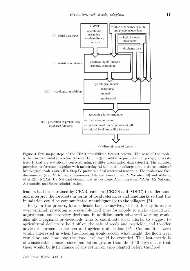
1–10 day flood forecasts. An example of the application of probabilisticenvironmental prediction is shown in figure 5. 10 day ensemble forecasts of theBrahmaputra River discharge at Bahadurabad are plotted against the forecasttarget date for the entire 2007 summer period. Two flooding events occurred(labelled I and II) during July and September, but no Ganges flooding (see[24] for details). Both flood events were forecast 10 days ahead quite accurately,both in the timing of the onset of the floods and their duration. The observeddischarge (the verification of the forecast) and matching the time of the forecastsis shown as a solid black line. The ensemble mean of the 10 day forecastappears as a white line. Estimates of flood risk at 5 and 10 day horizons,calculated from the spread of the plumes, are shown in figure 5b(i,ii). Both the5 and 10 day forecasts provided a very high probability of flooding at the correcttime and an accurate estimate of the duration of the flood. Forecasts for the otheryears of the Ganges and Brahmaputra 2004–2009 period are described in Websteret al. [24], along with a detailed assessment of skill.

Development of adaptation strategies. In 2007 and 2008,3 a number offlood-prone unions (equivalent to counties) along the Brahmaputra and theBrahmaputra–Ganges were chosen as test bed locations for applications of theflood forecasts (see fig. 1c, [24]). Advanced notice of each of the impending floodswas communicated by the FFWC to the unions and villages within the union bya planned cell-phone network and communicated within the villages by a series offlag alerts. In each union, government agriculture extension personnel and village3ADPC (http://www.adpc.net/v2007/) and the Centre for Environmental and GeographicInformation Services (CEGIS, http://www.cegisbd.com) are non-governmental organizationslocated in South Asia.

Phil. Trans. R. Soc. A (2011)

Prediction, risk, floods, adaption 11

downscaling of forecasts statistical correction

hydrological models

distributed

lumped

multi-model

generation of discharge forecast pdf

critical level probability forecast

(I) initial data input

(II) statistical rendering

(III) hydrological modelling

(IV) generation of probabilisticdischarge forecasts

ECMWF

operationalensemble

weather/climateforecasts

(V) dissemination of forecasts

NOAA & NASA satellite and precip. gauge data

accounting for uncertainties

hydrol model parameters

discharge data

final error correction

— —

—

—

——

—

—

—

—

—

—

—

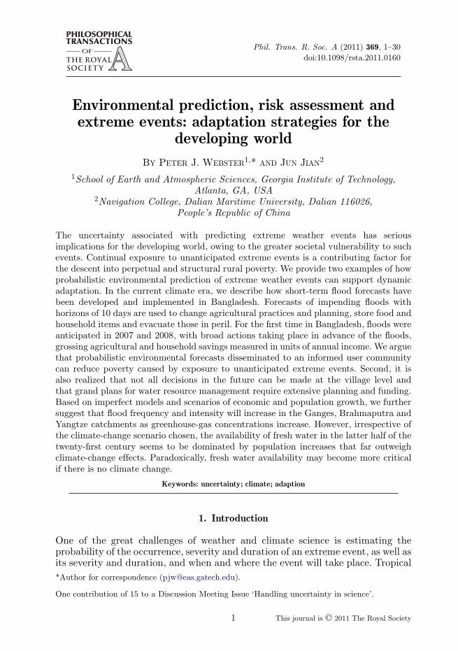
Figure 4. Five major steps of the CFAB probabilistic forecast scheme. The basis of the modelis the Environmental Prediction Scheme (EPS; [21]) quantitative precipitation (precip.) forecasts(step I) that are statistically corrected using satellite precipitation data (step II). The adjustedprecipitation forecasts, together with meteorological and initial discharge data initialize a suite ofhydrological models (step III). Step IV provides a final statistical rendering. The models are thendisseminated (step V) to user communities. Adapted from Hopson & Webster [23] and Websteret al. [24]. NOAA, US National Oceanic and Atmospheric Administration; NASA, US NationalAeronautics and Space Administration.

leaders had been trained by CFAB partners (CEGIS and ADPC) to understandand interpret the forecasts in terms of local references and landmarks so that theinundation could be communicated unambiguously to the villagers [24].

Early in the process, local officials had acknowledged that 10 day forecastswere optimal, providing a reasonable lead time for people to make agriculturaladjustments and property decisions. In addition, such advanced warning wouldalso allow regional professionals time to coordinate local efforts, to suggest toagricultural dealers to hold off on the sale of seeds and pesticide, and to offeradvice to farmers, fishermen and agricultural dealers [25]. Communities werevitally interested in when the flooding would occur, what height the flood levelwould be, and how long the flood level would be exceeded. This last metric isof considerable concern since inundation greater than about 10 days means thatthere would be little chance of any return on crop planted before the flood.

Phil. Trans. R. Soc. A (2011)

12 P. J. Webster and J. Jian

Q (

103

m3

s–1)

Q (

104

m3

s–1)

25 Ju

n8 J

ul

23 Ju

l

7 Aug

22 A

ug

21 S

ep6 S

ep6 O

ct

21 O

ct

14 Ju

l

20 Ju

l

26 Ju

l

1 Aug

11 A

ug

21 A

ug

31 A

ug5 S

ep

10 S

ep

15 S

ep

7 Aug

19 A

ug

13 A

ug

28 A

ug1 S

ep5 S

ep9 S

ep

13 S

ep

17 S

ep

21 S

ep

25 S

ep

29 S

ep

10 Ju

n5 J

ul

20 Ju

l

4 Aug

19 A

ug

18 S

ep3 S

ep

31 O

ct0

20

40

60

80

100

120

(a) (b)

forecast target date (2007)

0

20

40

60

80

100

I II

0

20

40

60

80

100

prob

abili

ty (

%)

10 day

5 day

10 day

5 day

10 day

5 day

date (2007)

(i) 10 day forecast

(ii) flood risk probabilities (period I)

(iii) flood risk probabilities (period II)

0

20

40

60

80

100pr

obab

ility

(%

)

date (2008)

0

20

40

60

80

100

flood level

flood period I

flood period II

(i) 10 day forecast

forecast target date (2008)

(ii) flood risk probabilities

Figure 5. The three left-hand panels in (a) refer to forecasts of Brahmaputra river discharge in2007, while the two right-hand panels in (b) refer to Brahmaputra flow in 2008. a(i) Summary ofthe 10 day Brahmaputra forecasts for the entire summer plotted against the forecast target data.(ii) Details of the period 13 July–19 August around the flood event I 27 July–6 August 2007 and28 August–30 September for flood II 7–17 September. a(ii)(iii), Flood exceedance probabilities forfloods I and II (27 July–6 August 2007 and 7–17 September, respectively). b(i) Same as (a), exceptfor 2008. (ii) Shows flood exceedance probabilities for the 5–10 September period, 2008. Adaptedfrom Hopson & Webster [23] and Webster et al. [24].

Phil. Trans. R. Soc. A (2011)

Prediction, risk, floods, adaption 13

A National Disaster Emergency Response Group planned the overall emergencyresponse and logistics for pre-flood preparedness and post-flood relief. Agencieswith local representation (e.g. Department of Agricultural Extension) preparedrehabilitation plans in advance for regions of high vulnerability. With the forecastof an impending flood, communities were advised to ‘wait, watch, worry and work’[24,25]. Evacuation assembly points were identified with adequate communicationand sanitation facilities. In the vulnerable regions, defined by the forecasts,fisheries were protected by increasing the height of the retaining netting aroundthe fishponds. Suggestions were made about harvesting crops early, ahead of theimpending flood or to delay planting. Families were advised to store about 10 daysworth of dry food and safe drinking water, as relief would not be forthcoming untilat least 7 days after the cessation of the flood. In addition, cattle and poultry,crop seed and portable belongings were to be secured in safe locations such ason road embankments. Of particular concern were the people of the river islands(or chars) farmed by the poorest of the poor that are rapidly engulfed by risingwater. Plans were made for the rapid deployment of manual and mechanizedboats for evacuation. With the normal 2–3 day FFWC forecast, these extensiveplans would have been impossible to implement; the 10 day forecasts producedby CFAB enabled adequate time to prepare properly for the floods [24].

Assessment of economic value of probabilistic forecasts. Following the floods,ADPC [25] assessed the utility of the 1–10 day forecasts, together with a cost–benefit analysis, by interviewing over 100 households. Although limited in scope,the survey indicated that there were substantial financial benefits in using theflood forecasts. It was estimated that the average savings for each householdinvolved in fisheries was equivalent to US$130, and in agriculture, it was US$190.The greatest savings per household were from the protection of livestock (US$500per cattle) and household assets (US$270 per household). Given that the averageincome in Bangladesh is approximately US$470 per year and that 50 per centof the population exists on less than US$1.25 per day [26], the savings weresubstantial in the flooded regions in terms of man-years of labour. For example,the loss of one cattle would require the equivalent of 2 man-years of labour forreplacement. The report concludes that the forecasts were accurate, timely andwell used in the pilot unions.

The utility of the forecasts is best summed by a statement made duringthe ADPC evaluation following the 2008 floods [25]. It also illustrates how theforecasts were incorporated into daily village life. As described by the Imamfrom the Mosque in Koijuri Union of Sirajgong District in Bangladesh: ‘Wedisseminate the forecast information and how to read the flag and flood pillar tounderstand the risk during the prayer time. In my field, T. Aman was at seedlingand transplanting stage, I used the flood forecast information for harvesting cropsand making decision for seedling and transplantation of T. Aman. Also we savedhousehold assets.’ (S. H. M. Fakhruddin 2010, personal communication.)

4. Adaptation to longer-term changes in extreme events

Three of the great rivers of South and East Asia, the Ganges, Brahmaputra andYangtze, currently support 14 per cent of the human population on the planet(figure 1), and are centres of thriving agrarian societies. During the next century,

Phil. Trans. R. Soc. A (2011)

14 P. J. Webster and J. Jian

this proportion of global population living in these river basins is expected to stayrelatively constant [27] supporting, in total, populations rising from 0.8 billion to1.5 billion.

Relatively strong relationships occur between total Indian rainfall and theEl Niño Southern Oscillation (ENSO) (e.g. [28–30] on interannual and decadalperiods, although this relationship has waned during the last few decades [31–36]). On longer time scales, Parthasarathy et al. [37,38] suggest that therehas been no significant long-term trend in the All-India rainfall index4 duringthe last 100 years, although there seems to be a weakening of the SouthAsian summer monsoon since the 1970s [40,41], though changes vary regionally[42]. With respect to Ganges and Brahmaputra floods, Jian et al. [43] foundprecursor relationships for Ganges discharge related broadly to the ENSO. Theseasonal Brahmaputra discharge, highly predictable at short forecast horizons[23,24], appeared to be only weakly linked to preceding SST anomalies, eitherremotely or regionally. However, Brahmaputra discharge was found to be stronglyand positively simultaneously correlated with simultaneous Indian Ocean SSTanomalies [43].

In a changing climate, it is important to assess the future distributions of thefrequency and severity of flooding in delta areas such as Bangladesh. A numberof studies have considered the impact of a doubling of CO2 on the monsooncirculation [44], on flooding [45–50] and on drought [51]. We attempt here todetermine the frequency, duration and severity of flooding in the Brahmaputra–Ganges delta during the next century using a selected number of climate modelsimulations. Specifically, we wish to determine whether the probability of floodand drought will change from the twentieth to the twenty-first centuries. A majorconcern is the availability of adequate fresh water during the next 100 years, whichis a function of both the rainfall as well and the population increase.

Methodology. We restrict our investigation to three main river basins: theBrahmaputra, Ganges and the Yangtze, based principally on the length ofavailable data (figure 3a). To assess possible changes in flood and drought risk,we have hydrological data for the last 50–60 years.

In addition to the river flow data, we use the Intergovernmental Panelon Climate Change (IPCC) fourth assessment report (AR4) [52] and coupledmodel intercomparison project phase three (CMIP3) simulations [53] to obtainestimates of future river flow. Most of the 25 coupled ocean–atmospheremodels were run in an ensemble mode for a three century period: the pre-industrial period, the twentieth century (in which historical values of greenhousegas (GHG) concentrations were incorporated) and the next 100 year usingprojections of GHG concentrations. These GHG concentration projectionsare made relative to a set of scenarios (described in the Special Reporton Emission Scenarios: SRES IPCC [54]). There are three basic familiesof SRES.

— GHG concentrations are assumed to hold constant at 2000 levels. We referto this as the GHG2000 scenario.

— The A-family set of scenarios that assumes rapid economical andtechnological growth with an increasing population in the first half of the

4The All-India rainfall index (AIRI) is a measure of the average rainfall over the entire Indiansub-continent [39].

Phil. Trans. R. Soc. A (2011)

Prediction, risk, floods, adaption 15

twenty-first century and a decreasing rate of growth in the second (A1) ora continuous growth rate of population throughout the century (A2). TheA-family projections range between CO2 concentrations of 700 and 1000ppm by the end of the century.

— The B-family of scenarios follow the A-family, except it is assumed thatthe economical structures of the planet are more environmentally sensitive,but with different population growth rates (B1 and B2). The A1B scenarioassumes similar growth to A1, but that there is a greater spread of energyproduction among non-fossil choices. Typical CO2 concentrations for theB-family are in the range 500–600 ppm by the end of the twenty-firstcentury.

Here, we consider four scenarios: GHG2000, B1, A1B, A1 and A2, thus spanningthe full IPCC SRES range.

A cautionary note should be made regarding scenario uncertainty. Thisuncertainty implies that it is not possible to formulate the probability ofoccurrence of one particular outcome. A scenario is a plausible but unverifiabledescription of how the system and/or its driving forces may develop in the future.Thus, scenarios should be regarded as a range of discrete possibilities with no apriori allocation of likelihood.

The IPCC AR4 notes that there is much less overall agreement amongmodels regarding changes in precipitation between models than with temperaturechanges (e.g. [55,56]). As river discharge depends critically on regionalprecipitation, it is clear that a different approach is needed in assessing futureriver flow. The approach has two components: model ‘culling’ and the use of aBayesian bias reduction technique.

Model culling. A critical problem is how to choose which model or combinationsof models from the CMIP-3 suite. Is the appropriate choice an average of allmodels and their families of ensembles to produce a multi-model, multi-ensemblemean as adopted by the IPCC? There are some benefits to this choice, asrandom error will tend to be eliminated by the averaging process. But thereis a downside too. Each model possesses regional systematic biases so that not allmodels will produce realistic fields of precipitation in all river basins, even for thepresent era.

We have developed a two-step process of minimizing systematic error inthe models.

— The models are rated relative to their ability to simulate the annual cycleof precipitation in the twentieth century in terms of magnitude and phasein a particular basin. This criterion is based on the observation that thethree river basins have strong annual cycles with a summer precipitationmaximum accounting for the majority of river flow.

— The annual precipitation of the three river basins are related to the phaseof the ENSO phenomena [57] that in turn is reflected in the river discharge.For example, the Ganges has a larger discharge during a La Niña year andless in an El Niño year. The discharge is marginally greater during a LaNiña year and considerably less during El Niño.

Phil. Trans. R. Soc. A (2011)

16 P. J. Webster and J. Jian

We choose these two selection criteria on the basis that unless these mostbasic physical ‘fingerprints’ are found in the model simulations, each related tofundamental forcing (i.e. the annual cycle of solar radiation and the largest SSTanomalies), then it would be unlikely that a reasonable estimate of river dischargecan be determined for the future. Of the two discriminators, the most importantis the ability of the model to possess an appropriate annual cycle in precipitation.

Examples of accepted and dismissed models based on the annual cycle andthe ENSO cycle are shown in figure 6. Figure 6a,b shows the observed riverdischarge and spatially averaged precipitation for the Ganges River basin forEl Niño and La Niña periods defined by a ±1 s.d. of central-eastern PacificOcean SSTs. Examples of CMIP-3 models not fulfilling these basic criteria are theBeijing Climate Center Climate Model (BCC-CM1; figure 6c(i)) and the InstitutePierre Simone Laplace (IPSL cm4; figure 6c(ii)). Examples of models fulfillingthe criteria are the German Max Planck Institute-ECHAM5 (figure 6d(i)) andthe UK Meteorological Office UKMO-HAD1 (figure 6d(ii)). Of the total of 25models, 13 passed the two tests for the Yangtze, 14 for the Ganges and 16 for theBrahmaputra.

Minimization of model bias. For those models that pass the two criteria, we needto apply a new mapping technique aimed at reducing model bias [57]. The systemadopted is similar to the q–q technique of Hopson & Webster [23] mentionedearlier in the paper for the short-term flood forecasting. The Bayesian techniquemaps multi-model precipitation estimates obtained from the twentieth centurysimulations with observed river discharge for each of the three rivers. Essentially, aq–q method maps the model-space precipitation and the observed-space dischargeof a particular river for each accepted model.

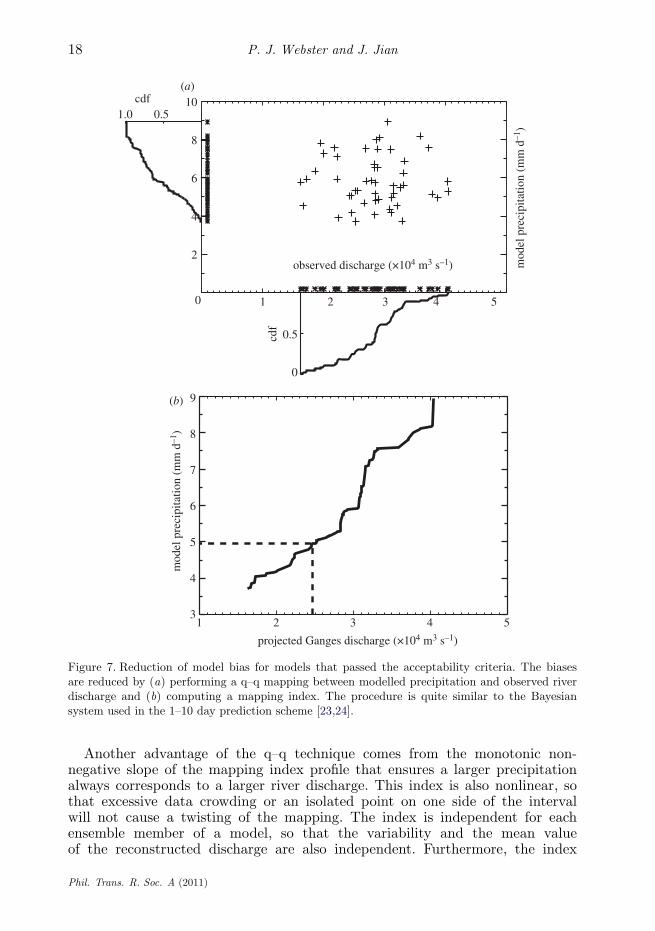
Cumulative density functions (cdfs) of both discharge-space and modelensemble member precipitation-space are calculated (figure 7a). Common overlapperiods are chosen for both the observed discharge and the simulated rainfall toensure that the same GHG domain is sampled. The observed discharge froma particular basin is separated into N equally spaced sequential intervals. Themodel rainfall for the particular basin is also divided into the same numberof intervals. An accumulated quantile value (cdf from 0 to 100) is calculatedby determining the percentage of data points that are less or greater than aparticular value. Then, the quantile points in model-space are mapped to the samequantile points in the observational-space (figure 7b). Thus, the observed 24thdischarge quantile of Yangtze River discharge (e.g.) is related to the 24th modelledprecipitation quantile generated for that period. This mapping technique removes,in essence, the model-to-model variability between the selected models.

The mapping index is constructed using the twentieth century simulatedprecipitation and observational river discharge (or gridded precipitation), both ofthem under the same influence of the twentieth century GHG radiative forcing. Inaddition, all four future SRES experiments are initialized directly from the endingstate of the climate of the same GHG2000 experiment as defined separately byeach model. As no other dynamic or thermal adjustments or forcing is used (otherthan the assumed growth of GHG concentrations under the various scenarios),it seems reasonable to apply the same ensemble-specific precipitation index tothe four SRESs to construct the future river discharges. The variability of themean river discharges is then most probably attributable to the different SRESscenarios.

Phil. Trans. R. Soc. A (2011)

Prediction, risk, floods, adaption 17

2 4 6 8 10 120

1

2

3

4

5

(i)

(i) (ii)

(ii)

(a)

(c)

(d)

(b)

disc

harg

e (×

104

m3

s–1)

2 4 6 8 10 120

5

10

pre

cipi

tatio

n (m

m d

–1)

2 4 6 8 10 120

5

10

15

mod

elle

d ra

infa

ll (m

m d

–1)

0 2 4 6 8 10 12

5

10

15

2 4 6 8 10 12month

0

5

10

15

mod

elle

d ra

infa

ll (m

m d

–1)

0 2 4 6 8 10 12month

5

10

15

Figure 6. Culling of the IPCC AR4 models AR4 models based on the precept that models thatsimulate the present era monsoon precipitation the best are most likely to perform better inestimating future monsoon precipitation. (a) Annual cycle of the Ganges River flow into Bangladesh(104 m3 s−1) measured at Hardinge Bridge. (b) Same as (a), except for rainfall (mm d−1) averagedover the Ganges catchment area upstream of Hardinge Bridge. (c) Examples of models that failedto replicate the annual cycle of precipitation over the Ganges catchment shown in (b). These modelswere (i) the Beijing Climate Center Climate model (BCC-CM1) and the Institute Pierre SimonLaplace climate model (IPSL cm4). (d) Two models that did replicate annual cycle of annualprecipitation shown in (a). These are (i) the Max Planck Institute ECHAM5 climate model and(ii) the UK Meteorological HAD1 climate model. In all figures, El Niño years are dashed lines, LaNiña years are dotted lines and normal years are solid lines.

Phil. Trans. R. Soc. A (2011)

18 P. J. Webster and J. Jian

1 2 3 4 50

2

4

6

8

10(a)

(b)

observed discharge (×104 m3 s–1) mod

el p

reci

pita

tion

(mm

d–1

)

0

0.5cdf

1.0 0.5cdf

1 2 3 4 5

projected Ganges discharge (×104 m3 s–1)

3

4

5

6

7

8

9

mod

el p

reci

pita

tion

(mm

d–1

)

Figure 7. Reduction of model bias for models that passed the acceptability criteria. The biasesare reduced by (a) performing a q–q mapping between modelled precipitation and observed riverdischarge and (b) computing a mapping index. The procedure is quite similar to the Bayesiansystem used in the 1–10 day prediction scheme [23,24].

Another advantage of the q–q technique comes from the monotonic non-negative slope of the mapping index profile that ensures a larger precipitationalways corresponds to a larger river discharge. This index is also nonlinear, sothat excessive data crowding or an isolated point on one side of the intervalwill not cause a twisting of the mapping. The index is independent for eachensemble member of a model, so that the variability and the mean valueof the reconstructed discharge are also independent. Furthermore, the index

Phil. Trans. R. Soc. A (2011)

Prediction, risk, floods, adaption 19

can be extended with linear interpolation on the ending points in case thefuture modelled precipitation output lies outside the current observed andmodelled space.

Flood risk probabilities in the twenty-first century. Figure 8a–c shows the resultsof the analysis of the qualified models following the q–q mapping for the Ganges,the Brahmaputra and the Yangtze for each of the four emission scenarios fromthe mid-nineteenth century through to the twenty-first century. The ‘plumes’represent the evolution of each of the sets of ensembles of the accepted models,colour coded relative to the particular SRES. The bold solid lines show theevolution of the multi-model mean and the plumes represent ±1 s.d. from themean. In general, the fixed CO2 concentration (GHG2000) shows a relativelyconstant mean value and about the same variability about the mean as duringthe twentieth century. This is a heartening result since it shows that this multi-model ensemble does not undergo model drift or dispersion. This result allows amore confident interpretation of the other experiments that do show change withtime, such as the B1, A1B and A2, with increasing mean values and an expandingspread over the next 100 years. Given the constancy of the spread of the GHG2000experiments, we can interpret the expanding dispersion of members as an increasein interannual variability. The largest increases occur with the A2 scenario withinwhich CO2 concentrations expand to 850 ppm by the end of the twenty-firstcentury. These results are consistent with the findings of Dairaku et al. [58].

Table 2 summarizes the statistics of the simulations. Discharges and standarddeviations (s.d.) are listed for each river basin and SRES scenario, includingGHG2000, for 25 year blocks between 2000 and 2099. Increases in discharge areprojected to occur between each quarter of the twenty-first century of the multi-model simulations. In the last quarter of the twenty-first century compared withobserved values for the twentieth century, one finds increases of 13 and 20 per centfor the Ganges, 15 and 30 per cent for the Brahmaputra and 10 and 19 per centfor the Yangtze, for the B1 and A32 scenarios. The s.d. for the observed twentiethcentury Brahmaputra discharge about the mean is 5704 m3 s−1. The s.d. for thelast quarter of the twenty-first century is 9605 m3 s−1. Thus, current observedmean discharge +1 s.d. (45 731 m3 s−1) does not exceed the mean value of the last25 years of the twenty-first century (50 413 m3 s−1).

If we assume that the streamflow producing a flood remains the same inthe next century as in the current era, we can calculate the probability offlood duration in the future. To determine the duration of flooding in thetwenty-first century, each ensemble member for a particular SRES was followed,and the duration of flood periods greater than a certain number of days wascalculated. Using occurrences of flooding in the Brahmaputra and the Gangesduring the second half of the twentieth century as the standard (table 1),the probability of flooding of a particular duration and return period can becalculated for each SRES considered. These results are shown in figure 9 forthe Ganges and Brahmaputra. The required daily data for the Yangtze is notavailable, although the increase in the mean and s.d. (figure 8c and table 2)is similar to the Ganges and Brahmaputra so that perhaps an extrapolationof the Brahmaputra and Ganges results to the Yangtze may be an adequateapproximation. Results are shown for the probabilities of 5 day and 10 day floods(left-hand ordinate) and return time of a flood of a particular duration (right-hand ordinate) plotted by year for the Ganges (dashed) and Brahmaputra (solid).

Phil. Trans. R. Soc. A (2011)

20 P. J. Webster and J. Jian

1850 1900 1950 2000 2050 2100 2150year

15

20

25

30

35

40

45(a)

(b)

(c)

mea

n di

scha

rge

(×10

3 m

3 s–1

)m

ean

disc

harg

e (×

103

m3

s–1)

mea

n di

scha

rge

(×10

3 m

3 s–1

)

1850 1900 1950 2000 2050 2100 2150year

30

35

40

45

50

55

60

65

1850 1900 1950 2000 2050 2100 2150year

30

35

40

45

50

55

60

65

Figure 8. Simulated discharge (×103 m3 s−1) over the next century of the (a) Ganges, (b)Brahmaputra and (c) Yangtze Rivers at the Hardinge Bridge and Bahadurabad in Bangladeshand Datong in China, respectively, for a range of SRESs, including the scenario when the CO2concentrations are held at the 2000 level. The multi-model ensemble means are shown as the boldlines. The twentieth century simulations are in black. The grey surroundings denote ±1 s.d. Theobserved fields for the three rivers are in purple, and show greater interannual variability thanthe twentieth century simulated fields. The twenty-first century SRES fields are shown (togetherwith ± 1 s.d.) as yellow (GHG2000), blue (B1), red (A2) and green (A1B). With the exception ofGHG2000, all the scenarios show increasing mean discharges and increasing variability with time.

Phil. Trans. R. Soc. A (2011)

Prediction, risk, floods, adaption 21

Table 2. Summary of modelled, observed and projected river discharges (102 m3 s−1) fromfigure 8a–c showing mean and standard deviation of the interannual series of river discharges(m3 s−1) from different SRES cases, the twentieth century experiment run, and the observations.Means and standard deviations for four 25 year periods (2000–2024, 2025–2049, 2050–2074, and2050–2099) are shown.

Ganges Brahmaputra Yangtze(102 m3 s−1) (102 m3 s−1) (102 m3 s−1)

observationstwentieth century 1951–2000 283 ± 57 400 ± 57 437 ± 72

simulationstwentieth century 1950–2000 283 ± 59 401 ± 59 438 ± 72twentieth century complete 282 ± 58 401 ± 60 439 ± 73

scenario periodGHG2000 2000–2024 291 ± 65 405 ± 63 429 ± 65

2025–2049 290 ± 63 400 ± 61 425 ± 642050–2074 285 ± 68 393 ± 60 432 ± 722075–2099 290 ± 65 411 ± 67 432 ± 79

B1 2000–2024 293 ± 65 415 ± 65 433 ± 732025–2049 307 ± 67 422 ± 67 447 ± 912050–2074 313 ± 71 441 ± 76 454 ± 832075–2099 315 ± 71 453 ± 78 473 ± 96

A1B 2000–2024 292 ± 62 411 ± 65 425 ± 702025–2049 310 ± 62 435 ± 75 442 ± 782050–2074 327 ± 65 475 ± 87 478 ± 1012075–2099 329 ± 68 498 ± 89 483 ± 100

A2 2000–2024 293 ± 65 407 ± 69 416 ± 672025–2049 294 ± 64 411 ± 72 425 ± 682050–2074 319 ± 66 450 ± 83 451 ± 832075–2099 342 ± 78 504 ± 96 502 ± 117

The twentieth century statistics are shown on the left-hand side of the figures.In the current era, the Ganges has a 15 per cent probability of a flood withduration greater than 5 days each year. The Brahmaputra is higher at 20 percent. Current probabilities of Ganges and Brahmaputra floods exceeding 10 daysare 12 and 8 per cent, respectively. For all scenarios, except the GHG2000 (whichshows steady probabilities throughout the twenty-first century), all probabilitiesincrease substantially through the twenty-first century. For example, A1B floodprobabilities increase by a factor of two for 5 day flooding and by a factor of fourfor the 10 day flooding. Return times of 10 day floods decreases by a factor ofthree by the end of the century, suggesting return periods of 2–3 years.

In summary, within the confines of confidence in the SRESs and modeluncertainties, Brahmaputra and Ganges flooding can expect more frequent longerduration flooding during the coming century. According to the model results, theseverity of the floods would also increase.

Drought probability. Determining potential river basin drought probabilitiesare critical for future water resource management. It may seem paradoxical toseek the probability of drought in an environment that may have an overall

Phil. Trans. R. Soc. A (2011)

22 P. J. Webster and J. Jian

75–99

10

20

30

40

50

(a) (b)2 yr

3 yr

4 yr

5 yr

10 yr

retu

rn p

erio

d (y

ears

)

year

10

20

30

40

50 2 yr

3 yr

4 yr

5 yr

10 yr

> 5 days > 10 dayspr

obab

ility

(%

)

50–99 00–24 25–49 50–75 75–99year

50–99 00–24 25–49 50–75

Figure 9. Flood probability (left ordinate) and return period (right ordinate) for floods of duration(a) more than 5 days and (b) more than 10 days for the Ganges (dashed line) and Brahmaputra(solid). Results for the GHG2000 (filled circles) and the A1B (open circles) scenarios are shown.The results for the observed period (1950–1999) are shown on the left of each panel, indicatingprobabilities of a more than 5 day (more than 10 day) flood of roughly 15–20% (10%) in anygiven year. These floods have current return periods of 5 and 10 years, respectively. Averageprobabilities and return periods in 25 year blocks are plotted to the right of the ordinate. For theconstant GHG concentrations, the probabilities and return periods remain the same for the nextcentury. But for the A1B scenario, probabilities increase to 40–50% for more than 5 day floods and30–40% for more than 10 day floods. According to the simulations, more than 10 day floods mayoccur biennially.

increase of precipitation. But, figure 8a–c suggests that there is considerable andincreasing variability about the mean discharge. Thus, it is possible that droughtevents may become more frequent. The situation may be exacerbated by increasedtemperature and evaporation.

In South Asia, drought events are determined by precipitation and evaporationrate increases, and the amount needed for society, industry and agriculture [51,59–61]. We adopt the most commonly used Indian drought index introduced by Sikka[62]. It is a simple meteorological monsoon drought metric determined directlyfrom the deficiency of seasonal rainfall. Moderate droughts and extreme droughtsare defined when the quantum of the seasonal rainfall deficits are more than −1.25and more than −2 s.d., respectively.

The probability of Ganges basin drought risk is summarized in table 3 forboth moderate and extreme events in the boreal summer and winter. In thepresent era, based on annual mean rainfall, moderate droughts have about a 10per cent probability and extreme events a much smaller chance of occurrence.Projections into the twenty-first century show no statistically significant changein the probability of a moderate or extreme drought, except perhaps for the A2scenario. That is, the probability of Brahmaputra and Ganges drought remainsmuch the same as the twentieth century probability, with perhaps a slightdecrease.

Phil. Trans. R. Soc. A (2011)

Prediction, risk, floods, adaption 23

Table 3. Meteorological drought probability (%) and return period of deficient precipitations underdifferent IPCC SRES scenarios for the Ganges Rivers. Numbers rounded to nearest whole number.The scenarios in the twenty-first century are divided into two periods (2000–2049 and 2050–2099).

Ganges River Basin drought probability (%) and return period (in years)moderate drought extreme drought(<mean −1.25 s.d.) (<mean −2 s.d.)

based on annual mean rainfall % years % years

observed (after 1950) 10 10 4 25twentieth century simulation 10 10 2 65

scenario periodfixed GHG 2000–2049 12 9 3 34

2050–2099 14 7 2 40B1 2000–2049 10 10 3 49

2050–2099 10 10 3 43A1B 2000–2049 13 8 3 51

2050–2099 10 10 3 47A2 2000–2049 13 8 2 43

2050–2099 9 12 2 41

Fresh water availability. Given probabilistic projections of river dischargethroughout the next century and a range of the projected population growth, it ispossible to make a broad-brush estimate of the availability of fresh water in each ofthe three basins. We calculate the total basin population based on the expectedcountry population [27], and assume that the ratio of the basin to the entirecountry population would stay at the year 1990 level throughout the twenty-first century. Total basin population, river discharge and fresh water per capitaare plotted in figure 10a–c for the A1, A2, B1 and GHG2000 scenarios.

Here, we equate river discharge with fresh water availability. Overall, the resultsof the analysis show that availability is driven almost exclusively by populationgrowth rather than by climate change. The 20–30% increases in mean riverdischarge (apparent in figure 8a–c) are almost irrelevant factors in the face ofprojected large population increases. This is particularly obvious in the A2 casethat, associated with large population increases, suggests a fresh water availabilitydecreasing by a factor of 1.5 in all three river basins. On the other hand, basinswill maintain fresh water supply per person at the current level under the A1/B1case, based on the assumed steadying or retreating of the population in themiddle and late parts of the twenty-first century. This is particularly evidentin the Yangtze basin. In figure 8, it was apparent that there was a low riskof river discharge change if the GHG levels are maintained at their presentlevels. Assuming that the population follows the A1 or B1 trajectories, it canbe seen that the fresh water depletion is greatest in each basin if there is noclimate change.

This analysis on the availability of fresh water is rather simplistic because itignores feedbacks that may occur with population if water availability per capitawere to diminish. However, it provides a first approximation that may be useful

Phil. Trans. R. Soc. A (2011)

24 P. J. Webster and J. Jian

1900 1950 2000year

2050 2100

A1 & B1

A2

0

50

100

150

200

250

300

basi

n po

pula

tion

(mill

ions

)

0

2000

4000

6000

8000

10 000

12 000

1900 1950 2000 2050 2100

A1 & B1

A2

0

200

400

600

800

1000(a)

(b)

(c)

basi

n po

pula

tion

(mill

ions

)

wat

er p

er c

apita

wat

er p

er c

apita

wat

er p

er c

apita

0

500

1000

1500

2000

2500

A1 B1

A2A1(2000)

A2(2000)

1900 1950 2000 2050 2100

A1 & B1

A2

0

200

400

600

800

basi

n po

pula

tion

(mill

ions

)

0

1000

2000

3000

A1 B1

A2

A1(2000)

A2(2000)

A1B1

A2

A1(2000)A2(2000)

Figure 10. Population (black curves, left-hand ordinate) for the A2, A1, B1 scenarios and freshwater availability (discharge per population; red curves, right-hand ordinate) for the twenty-firstcentury for the (a) Ganges, (b) Yangtze and (c) Brahmaputra River basins. Fresh water availabilityis dominated by projected population increases (solid red curves), and the increases in dischargeare largely irrelevant. Dashed red curves show fresh water availability for the GHG2000 for theA1, A2, and B1 population growth rates. In the latter case, fresh water availability decreasesmonotonically with time.

Phil. Trans. R. Soc. A (2011)

Prediction, risk, floods, adaption 25

for policy makers dealing with adaptation to a changing hydrological regime thatincludes both the impacts of climate change, no climate change and populationgrowth.

5. Summary

We have considered examples of how environmental prediction allows thedevelopment of risk management and adaptation strategies to deal with extremeevents that occur in the present climate era and those that may be encounteredduring the next century in the range of the IPCC SRESs. Strategies dependupon environmental prediction, but short-term adaptation is best handled atthe community level, whereas long-term adaptation requiring major engineeringinnovations may have to be handled bi-laterally or multi-laterally.

We have argued that the continual exposure to extreme events (floods,droughts, tropical cyclones) affecting communities every few years places familiesin economic jeopardy and should be considered as an important reason leadingto structural poverty. Furthermore, we have shown that some of the impactsare avoidable. Our fundamental hypothesis is that those who have experiencedcatastrophic loss owing to extreme events are those most adept at understandingrisk and developing adaptation strategies. For this reason we took probabilisticflood forecasts directly to the village level. Indeed, ADPC’s post-flood economicanalysis found averaging economic savings in households and farms that weremeasured in units of annual income.

Webster & Hoyos [63] offered another example of how environmental predictioncould have a very positive impact on the alleviation of poverty. They showedthat there was strong predictability of regional rainfall on the 20–25 day timescale. From an agricultural perspective, this prediction horizon is optimal andarguably far more important than information from a seasonal forecast, whichby necessity would be far less space and time specific. For example, a seasonalprecipitation forecast of the All-India Rainfall Index, as produced by the IndianMeteorological Department,5 is not regionally specific. Even a perfect forecastof an above or below average All-India Rainfall Index provides little help to thefarmer [63,64]. On the other hand, regional forecasts on the time scale of weeks,which provide relatively specific timing of precipitation events and dry periodson the spatial scale of Indian states, would allow farmers to optimize the timingof planting and harvesting. Webster and Hoyos argue that much of the crop lossin India in the very dry year of 2002 could have been avoided if 20 day forecastshad been available. Planting over much of India took place in an early wet spellthat was followed by a dry spell. Hoyos and Webster’s precipitation predictionsforecast the length of the dry spell and suggest that if general crop planting hadbeen delayed by 2 weeks, the impact of the disaster could have been mollifiedconsiderably.

In the developing world, there are two specific agro-hydrological regimes. Theseare the irrigated sectors and the rain-fed areas, the latter occupying 65–70% of allagriculture in the developing world. The advantage of irrigation is that availablewater in a particular sector comes from a wide collection area, so that even if a5Forecasts at http://www.imd.gov.in and also ‘Monsoon on Line’, http://www.tropmet.res.in/∼kolli/mol/Monsoon/frameindex.html.

Phil. Trans. R. Soc. A (2011)

26 P. J. Webster and J. Jian

particular region has depleted rainfall, water from areas receiving greater rainfallis available for agriculture. Multi-week forecasts, such as those of Webster &Hoyos, are of great utility even in an irrigated area, allowing water resourcemanagers to plan ahead and determine proportions of water storage used forpower generation or irrigation. As irrigation water is expensive, a rainfall forecastwill allow a farmer or a water manager in an irrigated area to plan out a wateringstrategy and optimize usage.

In a rain-fed region, there are far fewer options. The only available water isthat delivered locally by rainfall or, in some circumstances, from an artesiansource. In India, for example, areas of endemic rural poverty are located in rain-fed areas. Multi-week forecasts may allow an optimization of cropping in theselocations, enabling the reduction of the level of poverty. The use of probabilisticenvironmental predications for improving food security will be the subject of aseparate paper.

We also considered the role of environmental prediction for the developmentof adaptation strategies requiring long-term planning and large investment.These are central issues faced by governments as they plan for water resourcemanagement activities that may involve major construction (such as thedevelopment of fresh water storage and river diversion) and, at the same time,avoiding cross-border conflict. For example, China has made tentative plans todivert the Brahmaputra to irrigate the Gobi Desert region in Central Asia, aproposal that has caused great international concern in the region (see [65] fora discussion). India has been planning for the diversion of the Ganges and theBrahmaputra to allow irrigation of the currently rain-fed regions of India for along time. These plans, too, have raised international tensions between India andBangladesh (see [66] for a discussion). More recently, in Kashmir, hydroelectricschemes within India concern Pakistan [67]. Even if ‘spatial’ diversions of riversdo not take place and the dams are used for hydroelectricity, there may beproblems associated with ‘temporal’ diversion as water is withheld for periods tooptimize energy generation. During low winter flow periods, temporal diversionsmay have large impacts on irrigation in the lower reaches of basins. Rationaldecisions can only be made at national and international levels, taking intoaccount probabilities of climate change, population growth, the sustainabilityof agriculture and the needs of society downstream, provides, hopefully a widerange of viable options.

Using a range of climate model simulations, population estimates and GHGgrowth scenarios, it was suggested that there is a high probability of increasedriver discharge, especially in the last quarter of the twenty-first century. Also,flood frequency at all time scales increases with reduced return period. Droughts,though, do not appear to become more frequent, except in the winter season.Based on these imperfect models and the SRES scenarios, the future rangesfrom no change (with GHG concentrations held at 2000 levels) to more frequentfloods and a higher discharge in all three river basins (with A and B familyscenarios). If the higher probability of extreme events were to eventuate, povertywill be harder to alleviate without major infrastructure investment in watermanagement. Yet, in terms of the availability of fresh water, possibly the mostcritical factor facing the developing world is dominated by population growthand not climate change. Paradoxically, the greatest challenge to the three deltasin terms of fresh water availability considered occurs if there is no climate

Phil. Trans. R. Soc. A (2011)

Prediction, risk, floods, adaption 27

change during the next century. In summary, we have provided examples of howenvironmental prediction may help in the development of adaptation strategiesin the developing world. The incorporation of quantitative risk assessment intothe daily lives of diverse user groups can have the effect of minimizing propertyand income loss. It also provides a good adaptation strategy for future challengesassociated with climate change and increasing population. These challenges areserious. Obersteiner et al. [68] notes that societies may have to contend withnon-linear interactions between eco-systems and climate change. To this, we addthe complexity of population growth. Unattended, these interactions could leadto ‘…. sudden upward shift in the level of climate related damages and disastersthat finally result in civil unrest in some regions of the world as those societieslost their capacity to deal with the additional climate risk(s)…..’. Obersteineret al. [68, p. 12].

We dedicate this study to Sri A. Subbiah of ADPC and Mr T. Brennan, formerly of theUSAID Office of Foreign Disaster Assistance, who helped us understand problems at the villagelevel in the developing world. Funding from the National Science Foundation Climate DivisionGrant ATM-0531771 has enabled the development of the new predictive schemes and backgrounddiagnostic studies. We thank, in particular, Dr Jay Fein of NSF for allowing us to try andtranslate scientific ideas into something useful. Funding from CARE, USAID, the Georgia TechFoundation and an initial grant from the Climate and Societal Interactions Division of theNOAA Office of Global Programs made the implementation of the forecasts possible. We wishto thank the European Centre for Medium Range Weather Forecasts for the provision of theweather and climate ensemble products. CFAB depended on in-country collaboration for theeducation of users and the dissemination of the forecasts. This was accomplished by CEGISin Dhaka, Bangladesh, led by Ahmadul Hassan, and by S. H. M. Fakhruddin of ADPC inBangkok, Thailand, who were prepared to spend countless days risking their lives and healthin the flooded areas of Bangladesh working with communities to implement the forecasts.We are indebted to Dr J. A. Curry for her challenging questions and her comments on themanuscript.

References

1 Cuaresma, J. C., Hlouskova, J. & Obersteiner, M. 2008 Natural disasters as creativedestruction? Evidence from developing countries. Econ. Inquiry 46, 214–226. (doi:10.1111/j.1465-7295.2007.00063.x)

2 Toya, N. & Skidmore, M. 2007 Economic development and the impacts of natural disasters.Econ. Lett. 94, 20–25. (doi:10.1016/j.econlet.2006.06.020)

3 Webster, P. J. 2008 Myanmar’s deadly daffodil. Nat. Geosci. 1, 488–490. (doi:10.1038/ngeo257)4 Webster, P. J., Toma, V. E. & Kim, H.-M. 2011 Were the 2010 Pakistan floods predictable?

Geophys. Res. Lett. 38, L04806. (doi:10.1029/2010GL046346)5 Deodhar, R. 2003 A future without poverty: an idea book. See http://www.rahuldeodhar.com.6 Nickson, R., McArthur, J., Burgess, W., Ahmed, K. M., Ravenscroft, P. & Rahman, M. 1998

Arsenic poisoning of Bangladesh groundwater. Nature 395, 338–338. (doi:10.1038/26387)7 Smedley, P. L. & Kinniburgh, D. G. 2002 A review of the source, behaviour and distribution of

arsenic in natural waters. Appl. Geochem. 17, 517–568. (doi:10.1016/S0883-2927(02)00018-5)8 Nikolaidis, N. P., Dobbs, G. M. & Lackovic, J. A. 2003 Arsenic removal by zero-valent

iron: field, laboratory and modeling studies. Water Res. 37, 1417–1425. (doi:10.1016/S0043-1354(02)00483-9)

9 Central Intelligence Agency. 2010 Central Intelligence Agency ‘World-Factbook’. Seehttps://www.cia.gov/library/publications/the-world-factbook/.

10 Dhar, O. N. & Nandargi, S. 2000 A study of floods in the Brahmaputra basin inIndia. Int. J. Climate 20, 771–781. (doi:10.1002/1097-0088(20000615)20:7<771::AID-JOC518>3.0.CO;2-Z)

Phil. Trans. R. Soc. A (2011)

28 P. J. Webster and J. Jian

11 Central Water Commission. 2008 Annual Report 2007–2008. Central Water Commission,Ministry of Water Resources, Government of India. See http://www.cwc.nic.in/main/webpages/publications.html.

12 Jakobsen, F., Houque, A. K. M. Z., Paudyal, G. N. & Bhulyan, M. S. 2005 Evaluation ofshort-term processes forcing monsoon river floods in Bangldesh. Water. Int. 30, 389–399.(doi:10.1080/02508060508691880)

13 Mirza, M. M. Q., Warrick, R. A. & Ericksen, N. J. 2003 The implications of climate changeon floods of the Ganges, Brahmaputra and Meghna rivers in Bangladesh. Clim. Change 57,287–318. (doi:10.1023/A:1022825915791)

14 del Ninno, C. & Dorosh, P. A. 2001 Averting a food crisis: private imports and publictargeted distribution in Bangladesh after the 1998 flood. Agric. Econ. 25, 337–346. (doi:10.1016/S0169-5150(01)00090-1)

15 Streatfield, P. K. & Karar, Z. A. 2008 Population challenges for Bangladesh in the comingdecades. J. Health Popul. Nutr. 26, 261–272. (doi:10.3329/jhpn.v26i3.1894)

16 Smith, L. A. 2002 What might we learn from climate forecasts? Proc. Natl Acad. Sci. USA 99,2487–2492. (doi:10.1073/pnas.012580599)

17 Stainforth, D. A., Allen, M. R., Tredger, E. R. & Smith, L. A. 2007 Confidence, uncertaintyand decision support relevance in climate predictions. Phil. Trans. R. Soc. A 365, 2145–2161.(doi:10.1098/rsta.2007.2074)

18 Lorenz, E. N. 1963 Deterministic non-periodic flow. J. Atmos. Sci. 20, 130–141. (doi:10.1175/1520-0469(1963)020<0130:DNF>2.0.CO;2)

19 Palmer, T. N. 2000 Predicting uncertainty in forecasts of weather and climate. Rep. Progr.Phys. 63, 71–116. (doi:10.1088/0034-4885/63/2/201)

20 Leutbecher, M. & Palmer, T. N. 2008 Ensemble forecasting. J. Comput. Phys. 227, 3515–3539.(doi:10.1016/j.jcp.2007.02.014)

21 Molteni, F., Buizza, R., Palmer, T. N. & Petroliagis, T. 1996 The ECMWF ensembleprediction system: methodology and validation. Q. J. R. Meteorol. Soc. 122, 73–119.(doi:10.1002/qj.49712252905)

22 Anderson, D., Stockdale, T., Balmeseda, M., Ferranti, L., Vitart, F., Molteni, F., Doblas-Reyes, F., Mogensen, K. & Vitart, F. 2007 Development of the ECMWF seasonal forecastSystem 3. ECMWF Technical memorandum 503. See http://www.ecmwf.int/publications/library/do/references/show?id=87744.

23 Hopson, T. M. & Webster, P. J. 2010 A 1–10 day ensemble forecasting scheme for majorriver basins in Bangldeash: forecasting the severe floods of 2003–07. J. Hydromet. 11, 618–641.(doi:10.1175/2009JHM1006.1)

24 Webster, P. J. et al. 2010 Extended-range probabilistic forecasts of Ganges and Brahmaputrariver discharge. Bull. Amer. Meteorol. Soc. 91, 1493–1514. (doi:10.1175/2010BAMS2911.1)

25 ADPC. 2009 Flood Forecasts Application for Disaster Preparedness: Post Flood ForecastsAssessment 2008: community Response to CFAN Forecasts. See http://www.adpc.net/v2007/and http://pacific.eas.gatech.edu/∼pjw/FLOODS.

26 United Nations Children’s Fund 2010 United Nations Children’s Fund Country Statistics. Seehttp://www.unicef.org/infobycountry/.

27 Center for International Earth Science Information Network (CIESIN). 2002 Country-levelpopulation and downscaled projections based on the A1, B1 and A2 scenarios, 1990–2100 [digital version], Palisades, NY: CIESIN, Columbia University. See http://sedac.ciesin.columbia.edu/gpw.

28 Yasunari, T. 1990 Impact of Indian monsoon on the coupled atmosphere/ocean system in thetropical Pacific. Meteorol. Atmos. Phys. 44, 29–41. (doi:10.1007/BF01026809)

29 Shukla, J. & Paolina, D. A. 1983 The southern oscillation and long range forecasting ofthe summer monsoon rainfall over India. Mon. Weather Rev. 111, 1830–1837. (doi:10.1175/1520-0493(1983)111<1830:TSOALR>2.0.CO;2)

30 Shukla, J. 1995 Predictability of the tropical atmosphere, the tropical oceans and TOGA. InProceedings of the International Conference on the Tropical Ocean Global Atmopshere (TOGA)Programme, vol. 2, WCRP-91, pp. 725–730. Geneva, Switzerland: World Climate ResearchProgramme.

Phil. Trans. R. Soc. A (2011)

Prediction, risk, floods, adaption 29

31 Torrence, C. & Webster, P. J. 1998 The annual cycle of persistence in the El Niño-Southernoscillation. Q. J. R. Meteorol. Soc. 124, 1985–2004. (doi:10.1002/qj.49712455010)

32 Torrence, C. & Webster, P. J. 1999 Interdecadal changes in the ENSO-Monsoon System. J.Climate 12, 2679–2690. (doi:10.1175/1520-0442(1999)012<2679:ICITEM>2.0.CO;2)

33 Kumar, K. K., Rajagopalan, B. & Cane, M. A. 1999 On the weakening relationship betweenthe Indian monsoon and ENSO. Science 284, 2156–2159. (doi:10.1126/science.284.5423.2156)

34 Stephenson, D. B., Kumar, K. R., Dobias-Reyes, F., Royer, J. F., Chauvin, E. &Pezzulli, S. 1999 Extreme daily rainfall events and their impact on ensemble forecastsof the Indian Monsoon. Mon. Wea. Rev. 127, 1954–1966. (doi:10.1175/1520-0493(1999)127<1954:EDREAT>2.0.CO;2)

35 Clark, C. O., Cole, J. E. & Webster, P. J. 2000 SST and Indian summer rainfall: predictiverelationships and their decadal variability. J. Climate 13, 2503–2519. (doi:10.1175/1520-0442(2000)013<2503:IOSAIS>2.0.CO;2)

36 Clark, C. O., Webster, P. J. & Cole, J. E. 2003 The Indian Ocean dipole and theprediction of East African precipitation. J. Climate 16, 548–554. (doi:10.1175/1520-0442(2003)016<0548:IVOTRB>2.0.CO;2)

37 Parthasarathy, B., Munot, A. A. & Kothawale, D. R. 1995 The All-India monthly and seasonalrainfall series: 1871–1993. Theor. Appl. Clim. 49, 217–214. (doi:10.1007/BF00867461)

38 Parthasarathy, B., Diaz, H. F. & Eischeid, J. K. 1988 Prediction of All-India summer monsoonrainfall with regional and large-scale parameters. J. Geophys. Res. Atmos. 93, 5341–5350.(doi:10.1029/JD093iD05p05341)

39 Parthasarathy, B., Munot, A. A. & Kothawale, D. R. 1988 Regression model for estimation ofIndian foodgrain production from summer monsoon rainfall. Agric. For. Meteorol. 42, 167–182.(doi:10.1016/0168-1923(88)90075-5)

40 Webster, P. J., Magana, V. O., Palmer, T. N., Shukla, J., Tomas, R. A., Yanai, M. & Yasunari,T. 1998 Monsoons: processes, predictability, and the prospects for prediction. J. Geophys Res.103, 14 451–14 510. (doi:10.1029/97JC02719)

41 Wang, H. J. 2001 The weakening of the Asian monsoon circulation after the end of 1970’s. Adv.Atmos. Sci. 18, 376–386. (doi:10.1007/BF02919316)

42 Naidu, C. V., Durgalakshmi, K., Krishna, K. M., Rao, S. R., Satyanarayana, G. C.,Lakshminarayana, P. & Rao, L. M. 2009 Is summer monsoon rainfall decreasing in the globalwarming era? J. Geophys. Res. 114, D24108. (doi:10.1029/2008JD011288)

43 Jian, J., Webster, P. J. & Hoyos, C. 2009 Large-scale controls on Ganges and Brahmaputrariver discharge on intraseasonal and seasonal time scales. Q. J. R. Meteorol. Soc. 135, 353–370.(doi:10.1002/qj.384)

44 Kripalani, R. H., Oh, J. H. & Chaudhari, H. S. 2007 Response of the East Asian summermonsoon to doubled atmospheric CO2: coupled climate model simulations and projectionsunder IPCC AR4. Theor. Appl. Climatol. 87, 1–28. (doi:10.1007/s00704-006-0238-4)

45 Van Deursen, W. P. A. & Kwadijk, J. C. J. 1994 The impacts of climate change on the waterbalance of the Ganges-Brahmaputra and Yangtze Basin. Resource analysis report numberRA/94–160. See http://www.tudelft.nl/live/pagina.jsp?id=00bd4f3b-f76e-4603-aa23-84dbb31ce52&lang=en.

46 Milly, P. C. D., Wetherald, R. T., Dunne, K. A. & Delworth, T. L. 2002 Increasing risk of greatfloods in a changing climate. Nature 415, 514–517. (doi:10.1038/415514a)

47 Mirza, M. M. Q. 2002 Global warming and changes in the probability of occurrence offloods in Bangladesh and implications. Global Environ. Change 12, 127–138. (doi:10.1016/S0959-3780(02)00002-X)

48 Manabe, S., Milly, P. C. D. & Wetherald, R. 2004 Simulated long-term changes in river dischargeand soil moisture due to global warming. J. Sci. Hydrol. 49, 625–642. (doi:10.1623/husj.49.4.625.54.429)

49 Milly, P. C. D., Dunne, K. A. & Vecchia, A. V. 2005 Global pattern of trends in streamflowand water availability in a changing climate. Nature 438, 347–350. (doi:10.1038/nature04312)

50 Kleinen, T. & Petschel-Held, G. 2007 Integrated assessment of changes in flooding probabilitiesdue to climate change. Clim. Change 81, 283–312. (doi:10.1007/s10584-006-9159-6)

Phil. Trans. R. Soc. A (2011)

30 P. J. Webster and J. Jian

51 Kim, D. W. & Byun, H. R. 2009 Future pattern of Asian drought under global warming scenario.Theor. Appl. Climatol. 98, 137–150. (doi:10.1007/s00704-008-0100-y)

52 International Panel of Climate Change 2007 International Panel of Climate Change 4thAssessement. See http://www.ipcc.ch/.

53 Meehl, G. A., et al. 2007 The WCRP CMIP3 multimodel dataset: a new era in climate changeresearch, Bull. Am. Meteorol. Soc. 88, 1383–1394. (doi:10.1175/BAMS-88-9-1383)

54 SRES IPCC 2000 IPCC special report on emission scenarios (SRES), Summary for policymakers. See http://www.ipcc.ch/pdf/special-reports/spm/sres-en.pdf.

55 Palmer, T. N. & Räisänen, J. 2002 Quantifying risk of extreme seasonal prepcipitation eventsin a changing climate. Nature 415, 512–514. (doi:10.1038/415512a)

56 Räisänen, J. 2005 Impact of increasing CO2 on monthly-to-annual precipitation extremes:analysis of the CMIP2 experiments. Clim. Dyn. 24, 309–323. (doi:10.1007/s00382-004-0510-1)

57 Jian, J. 2007 Predictability of current and future multi-river discharge: the Ganges,Brahmaputra, Yangtze, Blue Nile and Murray-Darling Rivers. Georgia Institute of Technology,Atlanta, GA.

58 Dairaku, K., Emori, S. & Nozawa, T. 2008 Impacts of global warming on hydrological cyclesin the Asian Monsoon region. Adv. Atmos. Sci. 25, 960–973. (doi:10.1007/s00376-008-0960-1)

59 Mirza, M. M. Q. & Ahmad, Q. K. 2005 Climate change and water resources in South Asia, 1stedn. London, UK: Taylor & Francis.

60 Hirabayashi, Y., Kanae, S. & Emori, S. 2008 Global projections of changing risks of floods anddroughts in a changing climate. J. Sci. Hydrol. 53, 754–772. (doi:10.1623/hysj.53.4.754)

61 Sheffield, J. & Wood, E. F. 2008 Projected changes in drought occurrence under future globalwarming from multi-model, multi-scenario, IPCC AR4 simulations. Clim. Dyn. 31, 79–105.(doi:10.1007/s00382-007-0340-z)

62 Sikka, D. R. 1999 Monsoon drought in India. Joint COLA/CARE technical report no.2.See http://www.worldcat.org/search&qt=hotseries&q=se%3A%22Joint+COLA%2FCARE+technical+report%22.

63 Webster, P. J. & Hoyos, C. D. 2004 Prediction of monsoon rainfall and river discharge on 15–30day time scales. Bull. Am. Meteorol. Soc. 85, 1745–1765. (doi:10.1175/BAMS-85-11-1745)

64 Hoyos, C. & Webster, P. J. 2007 The role of intraseasonal variability in the nature of asianmonsoon rainfall. J. Climate 20, 4402–4424. (doi:10.1175/JCLI4252.1)

65 The Gaea Times 2010 Business News. See http://blog.taragana.com/business/2010/07/05/china-projects-wont-affect-brahmaputra-water-flow-minister-76230/.

66 National News 2003 National News. See http://search.com.bd/articles/bangladesh-india-water-problem.html.

67 New York Times 2010 See http://www.nytimes.com/2010/07/21/world/asia/21kashmir.html?r=1&emc=eta1.

68 Obersteiner, M., Azar, C., Kossmeier, S., Mechler, R., Möllersten, K., Nilsson, S., Read, P.,Yamagata, Y. & Yan, J. 2001 Managing climate risk. Interim report, International Institutefor Applied System Analysis Schlossplatz 1, A-2361, Laxenberg Austria. See http://www.iiasa.ac.at/Admin/PUB/Documents/IR-01-051.pdf.

Phil. Trans. R. Soc. A (2011)