environmentally-conscious highway design for vertical grades · environmentally-conscious highway...
TRANSCRIPT
Environmentally-Conscious Highway Design for Vertical Grades
by
Dr. Myunghoon Ko*
Texas A&M Transportation Institute
The Texas A&M University System
3135 TAMU
College Station, TX 77843-3135
Phone: (979) 847-6141
E-mail: [email protected]
Dr. Dominique Lord
Zachry Department of Civil Engineering
Texas A&M University, TAMU 3136
College Station, TX 77843-3136
Phone: (979) 458-3949
Fax: (979) 845-6481
E-mail: [email protected]
Dr. Josias Zietsman
Environment and Air Quality Division
Texas A&M Transportation Institute
The Texas A&M University System
3135 TAMU
College Station, TX 77843-3135
Phone: (979) 458-3476
Fax: (979) 845-7548
E-mail: [email protected]
October 29, 2012
Word Count: 5,499 + 3 Tables + 5 Figures = 7,499
*Corresponding author
ABSTRACT
This paper provides guidelines and tools for quantitative evaluations by means of fuel
consumption and emissions for various vertical grade design conditions. Detailed vehicle
operation conditions were represented by second-by-second speed profiles generated using the
truck dynamic model and non-uniform acceleration/deceleration models. The rates of fuel
consumption and emissions based on vehicle-specific power and speeds were extracted using
recently developed motor vehicle emission simulator (MOVES). The generated speed profiles
were matched with the extracted rates and aggregated during a trip on the grades. As a result, the
design vehicle consumed more than five times the amount of fuel on a 3,000-m graded segment
when the vehicle had a speed reduction of greater than 20 km/h, as opposed to the vehicle with a
speed reduction of less than 10 km/h. For emissions—carbon dioxide, carbon monoxide, oxides
of nitrogen, hydrocarbons, and particulate matter of 2.5 microns or less—there were up to five-
fold increases on the segment. Thus, controlling a speed reduction of less than 20 km/h can
minimize adverse environmental impacts from vehicle movements. In addition, this study shows
that environmentally-conscious vertical grade design is feasible and economically beneficial
throughout the life of the highway. The provided guidelines and tools can reduce uncertainty for
designing environmentally-conscious highways and can be used as part of the highway design
process.
Ko, Lord, and Zietsman 3
INTRODUCTION The intent of guidebooks or manuals used as part of the highway development process is to
permit sufficient flexibility for designers and engineers by providing a range or minimum values
for critical dimensions. Although documents, such as the Green Book (1), offer useful tools that
can help selecting the most appropriate design features, they do not provide specific information
about how the selected design features impact important external factors, such as those related to
crash risk and environmental emissions. In these cases, very often designers need to rely on
engineering judgment to make a final decision that balances direct and indirect costs, and
societal benefits. In order to reduce the uncertainty associated with engineering judgment,
AASHTO has recently published the Highway Safety Manual (2) among others. This Manual
provides tools and methods that allow practitioners to make planning, design, and operations
decisions based on safety. It is designed to facilitate explicit consideration of safety in the
decision making process.
Unfortunately, no such tools exist that explicitly consider environmental issues for
making highway design decisions. As discussed by Ko (3), even though there are several stages
that incorporate environmental analysis in this process, these analyses are usually conducted for
mobile emissions inventory prediction rather than for evaluating various geometric design
criteria. Research on concepts linked to environmentally-conscious highway geometric design is
still in its infancy, and highway design manuals/guidebooks do not provide any information
regarding the quantitative environmental impacts of highway geometric design features.
Therefore, including environmental factors in the highway design process is completely reliant
on engineering judgment. Guidelines are therefore needed to reduce the uncertainty linked with
engineering judgment.
The objectives of this paper are to 1) analyze the quantitative impacts of roadway grade
design features on fuel consumption and emissions; 2) show what degree of fuel consumption
and emissions can be changed by varying specific roadway grade design values with the
conceptual evaluation tool known as modification factors; and 3) propose practical methods and
processes of speed profiles and emissions rates for designers/engineers. The quantitatively
environmental research included in this paper can reduce uncertainty in engineering for
designing environmentally-conscious highways design. In addition, the research illustrates that
environmentally-friendly highway design can be one strategy that can be used to increase the
sustainability of transportation systems. This paper focuses only on vertical grade design; the
environmental evaluation of other design features can be found in two the other studies (3, 4).
BACKGROUND Examining the impact of vehicle operation conditions on fuel consumption and emissions, Servin
et al. (5) found that intelligent speed adaptation that regulates speed variation in driving
significantly saves fuel and reduced carbon dioxide (CO2) by approximately 37 percent and 35
percent, respectively. Existing research regarding the prediction of fuel consumption and
emissions uses vehicle speed expressed as a second-by-second variable. Average speed is not
adequate for evaluating the impacts of highway geometric design and traffic-signal control on
emissions and fuel consumption due to the lack of accounting for vehicle driving dynamics, such
as acceleration or deceleration (6, 7). Ahn et al. (8) and Qi et al. (7) developed microscopic
emissions models that predict vehicle fuel consumption and emissions using instantaneous speed
and acceleration/deceleration as explanatory variables. These models more accurately predict
fuel consumption and emissions compared to measured data.
Ko, Lord, and Zietsman 4
Roadway grade is one of the key variables affecting fuel consumption and emissions, as
are vehicle speed and acceleration. According to Boriboonsomsin and Barth (9), a vehicle
consumes 15 to 20 percent more fuel on an uphill segment at a 6-percent grade followed by
downhill segment at a 6-percent grade than on flat section of equal length. The larger amount of
fuel consumed going uphill is not fully compensated for by the smaller amount of fuel
consumption going downhill. Boriboonsomsin and Barth (9) concluded that speed and
acceleration have a large impact on vehicle fuel consumption and emissions. They found that
roadway grade is one of the primary variables that determine the power requirements necessary
for specific driving maneuvers. The aggregated emissions and fuel consumption based on the
second-by-second speed profile, including acceleration and roadway grades, can be used to
represent an inventory of emissions and fuel consumption related to highway geometric design
features.
METHODOLOGY This section describes the non-uniform acceleration models used to obtain second-by-second
speed profiles along roadway grade design features. Fuel consumption and emissions rates from
the mobile emissions model are then matched with the generated speed profiles, and calculated
emissions per second are aggregated along traveled distance and time.
Non-Uniform Acceleration/Deceleration Models
Non-uniform acceleration/deceleration models can be categorized into vehicle kinematics
models and vehicle dynamics models (10). The vehicle kinematics model predicts vehicle
acceleration from simplified mathematical relationships with speed and distance; however, it
does not account for vehicle type and mass, roadway grades, and other factors affecting vehicle
accelerating capacity (10). The vehicle dynamic model, on the other hand, predicts vehicle
acceleration from such factors.
The vehicle dynamics model is used for creating the second-by-second vehicle speed
profile related to roadway vertical grades; the calculated second-by-second speeds and
accelerations are used for estimating fuel consumption and emissions. Roadway vertical grade
design features are based on a typical heavy truck weighing 120 kg/kW, because the effect of
grades is more critical for a truck movement than for a passenger car (1). Generally, all
passenger cars can negotiate grades as steep as 4 to 5 percent without any significant speed
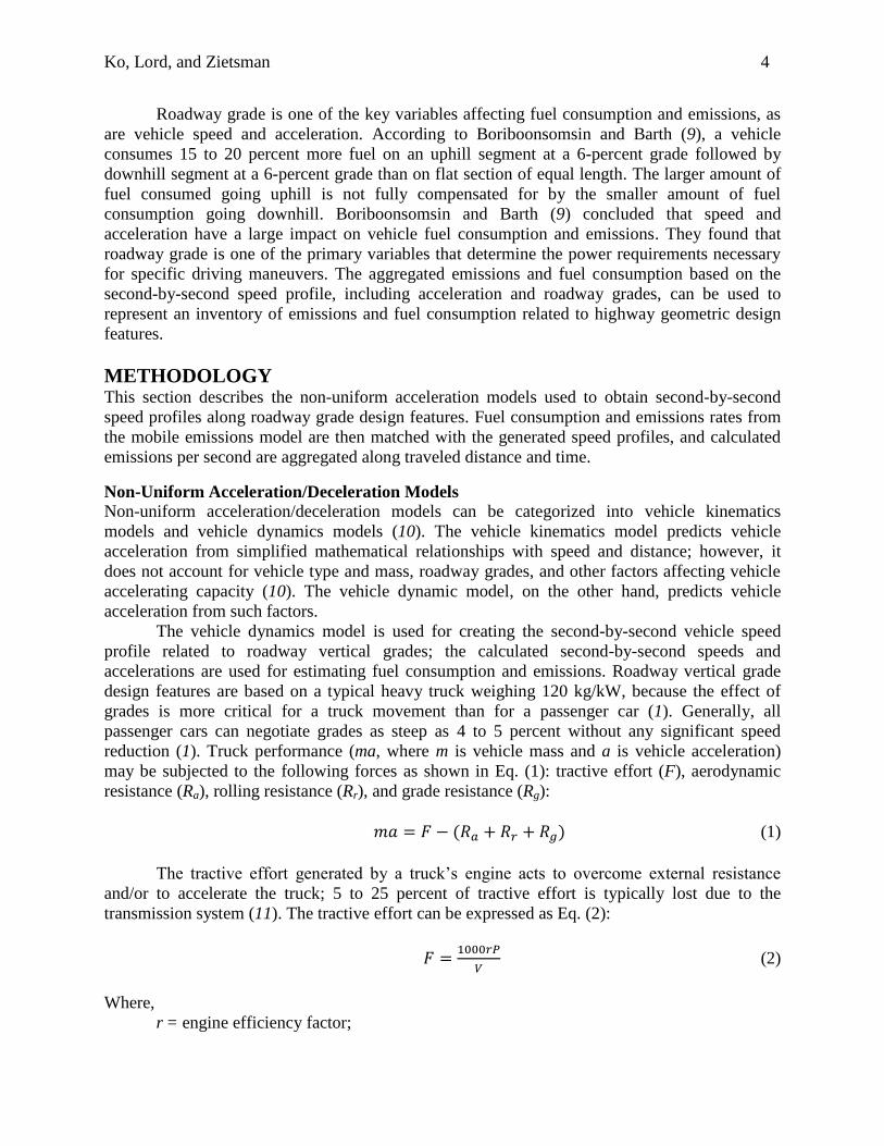
reduction (1). Truck performance (ma, where m is vehicle mass and a is vehicle acceleration)
may be subjected to the following forces as shown in Eq. (1): tractive effort (F), aerodynamic
resistance (Ra), rolling resistance (Rr), and grade resistance (Rg):
(1)
The tractive effort generated by a truck’s engine acts to overcome external resistance
and/or to accelerate the truck; 5 to 25 percent of tractive effort is typically lost due to the
transmission system (11). The tractive effort can be expressed as Eq. (2):
(2)
Where,
r = engine efficiency factor;
Ko, Lord, and Zietsman 5
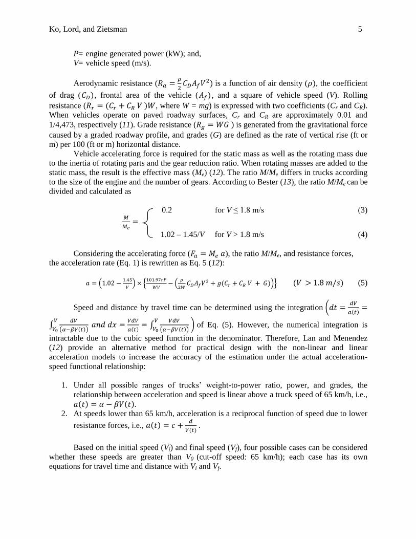
P= engine generated power (kW); and,
V= vehicle speed (m/s).
Aerodynamic resistance (
is a function of air density ( , the coefficient
of drag ( , frontal area of the vehicle ( , and a square of vehicle speed (V). Rolling
resistance ( , where W = mg) is expressed with two coefficients (Cr and CR).
When vehicles operate on paved roadway surfaces, Cr and CR are approximately 0.01 and
1/4,473, respectively (11). Grade resistance ( ) is generated from the gravitational force
caused by a graded roadway profile, and grades (G) are defined as the rate of vertical rise (ft or
m) per 100 (ft or m) horizontal distance.
Vehicle accelerating force is required for the static mass as well as the rotating mass due
to the inertia of rotating parts and the gear reduction ratio. When rotating masses are added to the
static mass, the result is the effective mass (Me) (12). The ratio M/Me differs in trucks according
to the size of the engine and the number of gears. According to Bester (13), the ratio M/Me can be
divided and calculated as
0.2 for V ≤ 1.8 m/s (3)
1.02 – 1.45/V for V > 1.8 m/s (4)
Considering the accelerating force ( ), the ratio M/Me, and resistance forces,
the acceleration rate (Eq. 1) is rewritten as Eq. 5 (12):
(
) {
(
)} (5)
Speed and distance by travel time can be determined using the integration (
∫
( )
∫
( )
) of Eq. (5). However, the numerical integration is
intractable due to the cubic speed function in the denominator. Therefore, Lan and Menendez
(12) provide an alternative method for practical design with the non-linear and linear
acceleration models to increase the accuracy of the estimation under the actual acceleration-
speed functional relationship:
1. Under all possible ranges of trucks’ weight-to-power ratio, power, and grades, the
relationship between acceleration and speed is linear above a truck speed of 65 km/h, i.e.,
2. At speeds lower than 65 km/h, acceleration is a reciprocal function of speed due to lower
resistance forces, i.e.,
.
Based on the initial speed (Vi) and final speed (Vf), four possible cases can be considered
whether these speeds are greater than V0 (cut-off speed: 65 km/h); each case has its own
equations for travel time and distance with Vi and Vf.
Ko, Lord, and Zietsman 6
Case I: Vi ≥ V0 and Vf ≥ V0
(
) (6)
(
) (7)
Case II: Vi ≤ V0 and Vf ≤ V0
(
) (8)
(
) (9)
Case III: Vi ≥ V0 and Vf ≤ V0
(
)
(
) (10)
(
)
(
) (11)
Case IV: Vi ≤ V0 and Vf ≥ V0
(
)
(
) (12)
(
)
(
) (13)
Motor Vehicle Emission Simulator (MOVES)
MOVES is the U.S. Environmental Protection Agency’s (EPA) state-of-the-art tool for
estimating fuel consumption and emissions from vehicle operations. MOVES incorporates large
amounts of in-use data from a variety of sources based on the analyses of emissions test results
and generates fuel consumption and emissions rates based on 23 operating mode bins with
instantaneous vehicle speeds and VSPs. The fuel consumption and emissions rates are based on
the condition provided in Table 1. Fuel consumption and emissions are aggregated during travel
time based on second-by-second operating mode bins from speed profiles and rates for each
operating mode bin.
∑ (14)
Where,
Etype = total emissions each for CO2, NOx, CO, HC, and PM2.5 or total fuel
consumption; and
Ko, Lord, and Zietsman 7
etype, bin, t = fuel consumption or emissions rate for type (i.e., passenger car and heavy-
duty truck) and operating bin at time t.
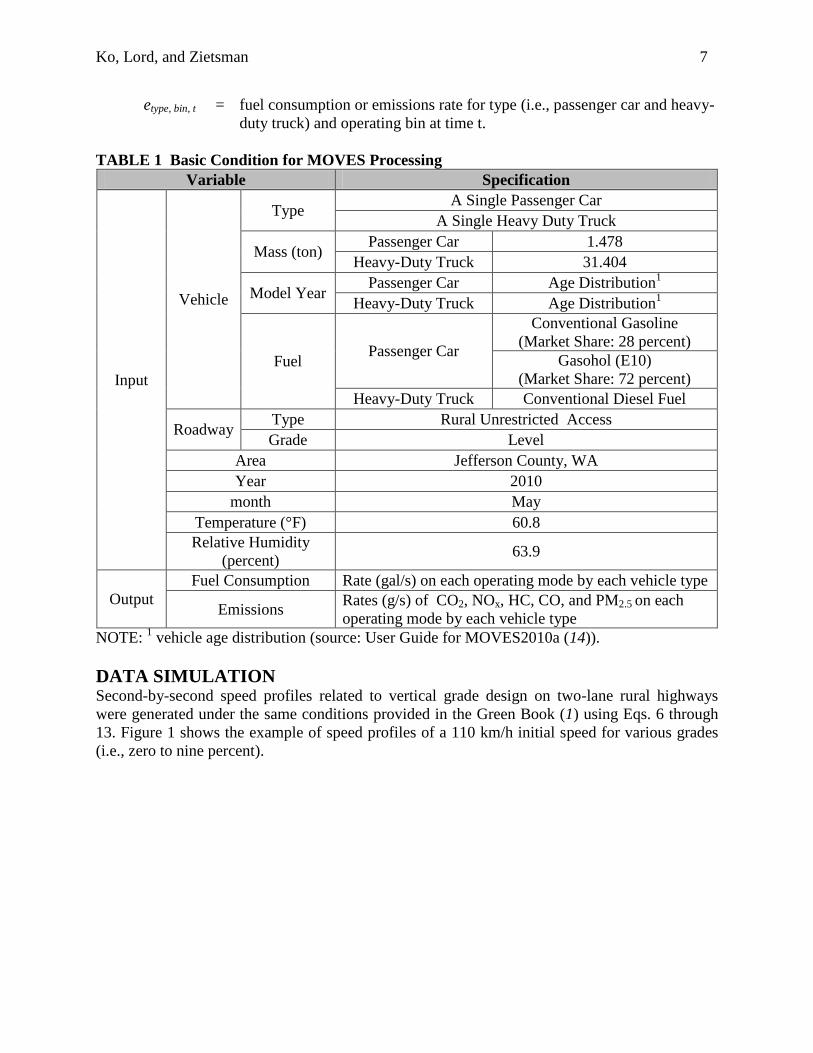
TABLE 1 Basic Condition for MOVES Processing
Variable Specification
Input
Vehicle
Type A Single Passenger Car
A Single Heavy Duty Truck
Mass (ton) Passenger Car 1.478
Heavy-Duty Truck 31.404
Model Year Passenger Car Age Distribution
1
Heavy-Duty Truck Age Distribution1
Fuel Passenger Car
Conventional Gasoline
(Market Share: 28 percent)
Gasohol (E10)
(Market Share: 72 percent)
Heavy-Duty Truck Conventional Diesel Fuel
Roadway Type Rural Unrestricted Access
Grade Level
Area Jefferson County, WA
Year 2010
month May
Temperature (°F) 60.8
Relative Humidity
(percent) 63.9
Output
Fuel Consumption Rate (gal/s) on each operating mode by each vehicle type
Emissions Rates (g/s) of CO2, NOx, HC, CO, and PM2.5 on each
operating mode by each vehicle type
NOTE: 1 vehicle age distribution (source: User Guide for MOVES2010a (14)).
DATA SIMULATION Second-by-second speed profiles related to vertical grade design on two-lane rural highways
were generated under the same conditions provided in the Green Book (1) using Eqs. 6 through
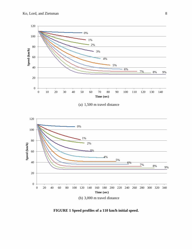
13. Figure 1 shows the example of speed profiles of a 110 km/h initial speed for various grades
(i.e., zero to nine percent).
Ko, Lord, and Zietsman 8
(a) 1,500 m travel distance
(b) 3,000 m travel distance
FIGURE 1 Speed profiles of a 110 km/h initial speed.
0%
1%
2%
3%
5%
6% 7% 8%
4%
9%
0
20
40
60
80
100
120
0 10 20 30 40 50 60 70 80 90 100 110 120 130 140
Sp
eed
(k
m/h
)
Time (sec)
0%
1%
2%
3%
4% 5%
6% 7% 8% 9%
0
20
40
60
80
100
120
0 20 40 60 80 100 120 140 160 180 200 220 240 260 280 300 320 340
Sp
eed
(k
m/h
)
Time (sec)
Ko, Lord, and Zietsman 9
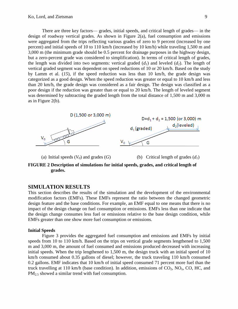
There are three key factors— grades, initial speeds, and critical length of grades— in the
design of roadway vertical grades. As shown in Figure 2(a), fuel consumption and emissions
were aggregated from the trips reflecting various grades of zero to 9 percent (increased by one
percent) and initial speeds of 10 to 110 km/h (increased by 10 km/h) while traveling 1,500 m and
3,000 m (the minimum grade should be 0.5 percent for drainage purposes in the highway design,
but a zero-percent grade was considered to simplification). In terms of critical length of grades,
the length was divided into two segments: vertical graded (d1) and leveled (d2). The length of
vertical graded segment was dependent on speed reductions of 10 or 20 km/h. Based on the study
by Lamm et al. (15), if the speed reduction was less than 10 km/h, the grade design was
categorized as a good design. When the speed reduction was greater or equal to 10 km/h and less
than 20 km/h, the grade design was considered as a fair design. The design was classified as a
poor design if the reduction was greater than or equal to 20 km/h. The length of leveled segment
was determined by subtracting the graded length from the total distance of 1,500 m and 3,000 m
as in Figure 2(b).
(a) Initial speeds (V0) and grades (G) (b) Critical length of grades (d1)
FIGURE 2 Description of simulations for initial speeds, grades, and critical length of
grades.
SIMULATION RESULTS This section describes the results of the simulation and the development of the environmental
modification factors (EMFs). These EMFs represent the ratio between the changed geometric
design feature and the base conditions. For example, an EMF equal to one means that there is no
impact of the design change on fuel consumption or emissions. EMFs less than one indicate that
the design change consumes less fuel or emissions relative to the base design condition, while
EMFs greater than one show more fuel consumption or emissions.
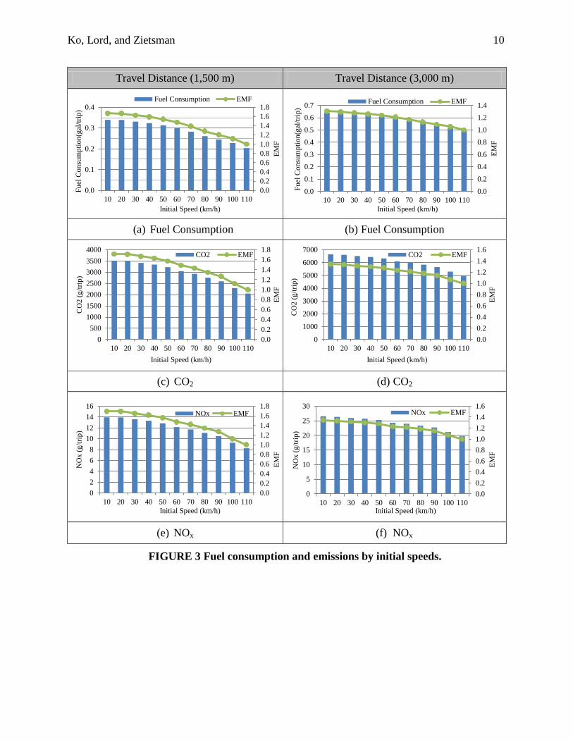
Initial Speeds
Figure 3 provides the aggregated fuel consumption and emissions and EMFs by initial
speeds from 10 to 110 km/h. Based on the trips on vertical grade segments lengthened to 1,500
m and 3,000 m, the amount of fuel consumed and emissions produced decreased with increasing
initial speeds. When the trip lengthened to 1,500 m, the design truck with an initial speed of 10
km/h consumed about 0.35 gallons of diesel; however, the truck traveling 110 km/h consumed
0.2 gallons. EMF indicates that 10 km/h of initial speed consumed 71 percent more fuel than the
truck travelling at 110 km/h (base condition). In addition, emissions of CO2, NOx, CO, HC, and
PM2.5 showed a similar trend with fuel consumption.
Ko, Lord, and Zietsman 10
Travel Distance (1,500 m) Travel Distance (3,000 m)
(a) Fuel Consumption (b) Fuel Consumption
(c) CO2 (d) CO2
(e) NOx (f) NOx
FIGURE 3 Fuel consumption and emissions by initial speeds.
0.0
0.2
0.4
0.6
0.8
1.0
1.2
1.4
1.6
1.8
0.0
0.1
0.2
0.3
0.4
10 20 30 40 50 60 70 80 90 100 110
EM
F
Fu
el C
on
sum
pti
on
(gal
/tri
p)
Initial Speed (km/h)
Fuel Consumption EMF
0.0
0.2
0.4
0.6
0.8
1.0
1.2
1.4
0.0
0.1
0.2
0.3
0.4
0.5
0.6
0.7
10 20 30 40 50 60 70 80 90 100 110
EM
F
Fu
el C
on
sum
pti
on
(gal
/tri
p)
Initial Speed (km/h)
Fuel Consumption EMF
0.0
0.2
0.4
0.6
0.8
1.0
1.2
1.4
1.6
1.8
0
500
1000
1500
2000
2500
3000
3500
4000
10 20 30 40 50 60 70 80 90 100 110
EM
F
CO
2 (
g/t
rip
)
Initial Speed (km/h)
CO2 EMF
0.0
0.2
0.4
0.6
0.8
1.0
1.2
1.4
1.6
0
1000
2000
3000
4000
5000
6000
7000
10 20 30 40 50 60 70 80 90 100 110
EM
F
CO
2 (
g/t
rip
)
Initial Speed (km/h)
CO2 EMF
0.0
0.2
0.4
0.6
0.8
1.0
1.2
1.4
1.6
1.8
0
2
4
6
8
10
12
14
16
10 20 30 40 50 60 70 80 90 100 110
EM
F
NO
x (
g/t
rip
)
Initial Speed (km/h)
NOx EMF
0.0
0.2
0.4
0.6
0.8
1.0
1.2
1.4
1.6
0
5
10
15
20
25
30
10 20 30 40 50 60 70 80 90 100 110
EM
F
NO
x (
g/t
rip
)
Initial Speed (km/h)
NOx EMF
Ko, Lord, and Zietsman 11
Travel Distance (1,500 m) Travel Distance (3,000 m)
(g) CO (h) CO
(i) HC (j) HC
(k) PM2.5 (l) PM2.5
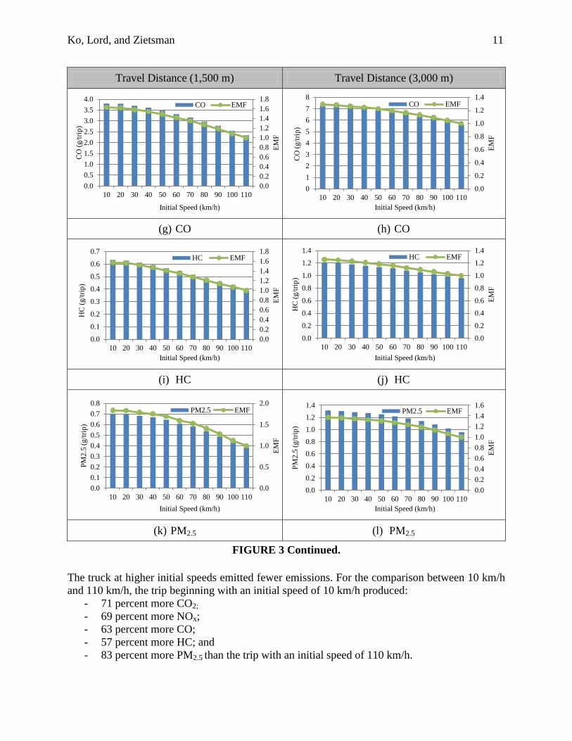
FIGURE 3 Continued.
The truck at higher initial speeds emitted fewer emissions. For the comparison between 10 km/h
and 110 km/h, the trip beginning with an initial speed of 10 km/h produced:
- 71 percent more CO2;
- 69 percent more NOx;
- 63 percent more CO;
- 57 percent more HC; and
- 83 percent more PM2.5 than the trip with an initial speed of 110 km/h.
0.0
0.2
0.4
0.6
0.8
1.0
1.2
1.4
1.6
1.8
0.0
0.5
1.0
1.5
2.0
2.5
3.0
3.5
4.0
10 20 30 40 50 60 70 80 90 100 110
EM
F
CO
(g/t
rip
)
Initial Speed (km/h)
CO EMF
0.0
0.2
0.4
0.6
0.8
1.0
1.2
1.4
0
1
2
3
4
5
6
7
8
10 20 30 40 50 60 70 80 90 100 110
EM
F
CO
(g/t
rip
)
Initial Speed (km/h)
CO EMF
0.0
0.2
0.4
0.6
0.8
1.0
1.2
1.4
1.6
1.8
0.0
0.1
0.2
0.3
0.4
0.5
0.6
0.7
10 20 30 40 50 60 70 80 90 100 110
EM
F
HC
(g/t
rip
)
Initial Speed (km/h)
HC EMF
0.0
0.2
0.4
0.6
0.8
1.0
1.2
1.4
0.0
0.2
0.4
0.6
0.8
1.0
1.2
1.4
10 20 30 40 50 60 70 80 90 100 110
EM
F
HC
(g/t
rip
)
Initial Speed (km/h)
HC EMF
0.0
0.5
1.0
1.5
2.0
0.0
0.1
0.2
0.3
0.4
0.5
0.6
0.7
0.8
10 20 30 40 50 60 70 80 90 100 110
EM
F
PM
2.5
(g/t
rip
)
Initial Speed (km/h)
PM2.5 EMF
0.0
0.2
0.4
0.6
0.8
1.0
1.2
1.4
1.6
0.0
0.2
0.4
0.6
0.8
1.0
1.2
1.4
10 20 30 40 50 60 70 80 90 100 110E
MF
PM
2.5
(g/t
rip
)
Initial Speed (km/h)
PM2.5 EMF
Ko, Lord, and Zietsman 12
During the 3,000 m trip, the truck consumed 34 percent more fuel and produced up to 37
percent more emissions at an initial speed of 10 km/h than at a speed of 110 km/h. Based on the
fuel consumption and emissions from the initial speed, the truck consumed less fuel and
produced less pollution at higher speeds.
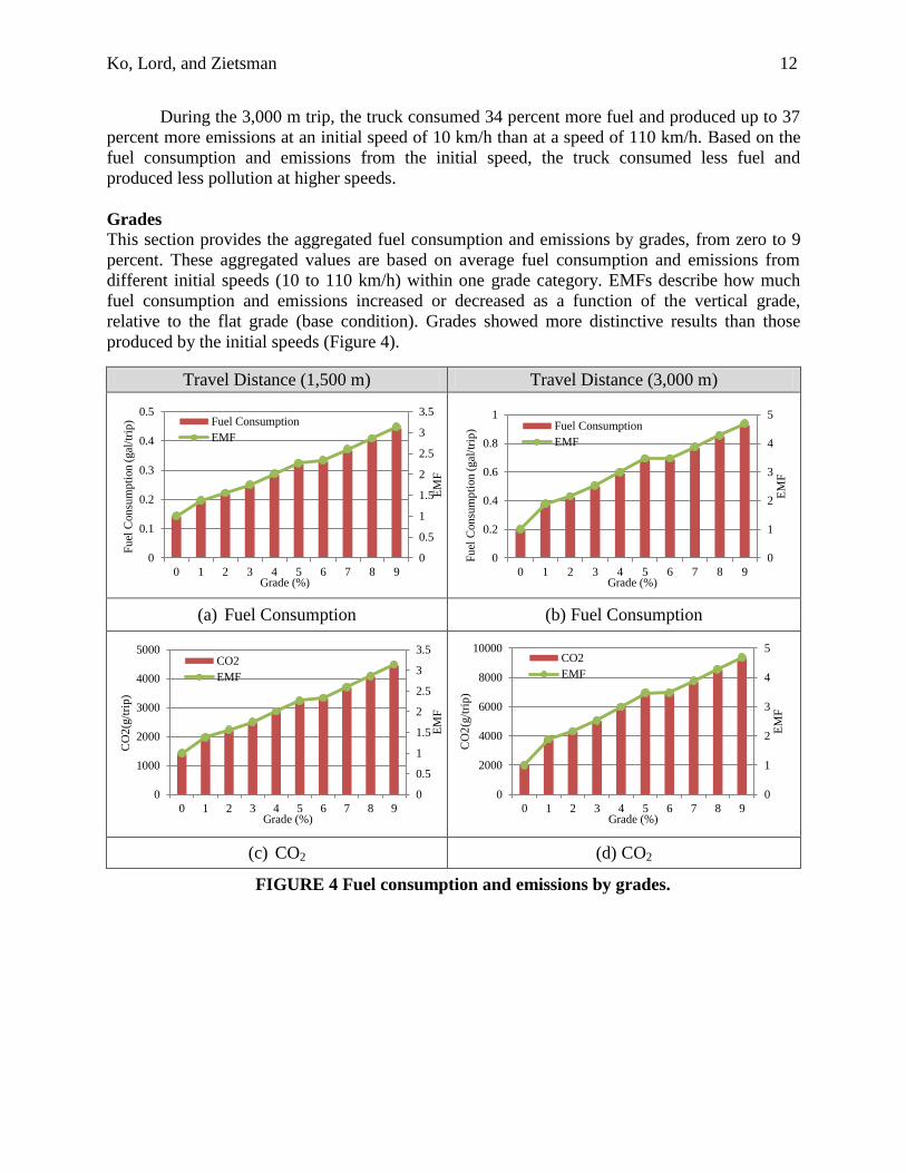
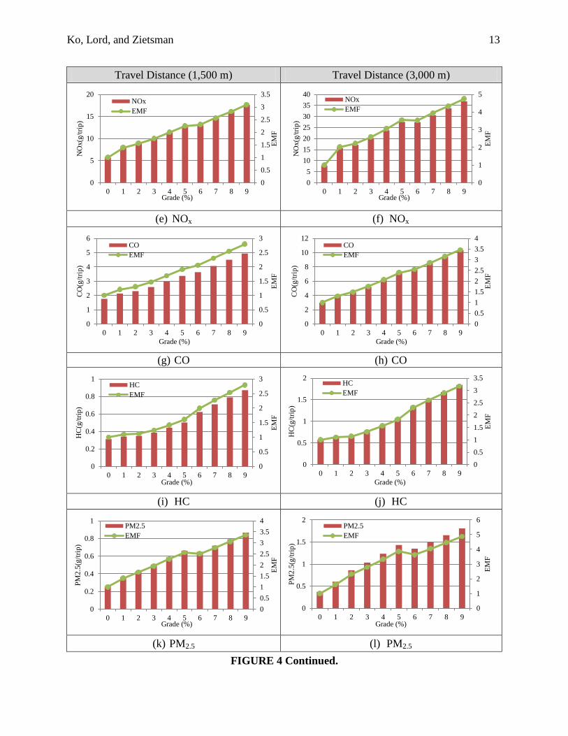
Grades
This section provides the aggregated fuel consumption and emissions by grades, from zero to 9
percent. These aggregated values are based on average fuel consumption and emissions from
different initial speeds (10 to 110 km/h) within one grade category. EMFs describe how much
fuel consumption and emissions increased or decreased as a function of the vertical grade,
relative to the flat grade (base condition). Grades showed more distinctive results than those
produced by the initial speeds (Figure 4).
Travel Distance (1,500 m) Travel Distance (3,000 m)
(a) Fuel Consumption (b) Fuel Consumption
(c) CO2 (d) CO2
FIGURE 4 Fuel consumption and emissions by grades.
0
0.5
1
1.5
2
2.5
3
3.5
0
0.1
0.2
0.3
0.4
0.5
0 1 2 3 4 5 6 7 8 9
EM
F
Fu
el C
on
sum
pti
on
(gal
/tri
p)
Grade (%)
Fuel Consumption
EMF
0
1
2
3
4
5
0
0.2
0.4
0.6
0.8
1
0 1 2 3 4 5 6 7 8 9
EM
F
Fu
el C
on
sum
pti
on
(gal
/tri
p)
Grade (%)
Fuel Consumption
EMF
0
0.5
1
1.5
2
2.5
3
3.5
0
1000
2000
3000
4000
5000
0 1 2 3 4 5 6 7 8 9
EM
F
CO
2(g
/tri
p)
Grade (%)
CO2
EMF
0
1
2
3
4
5
0
2000
4000
6000
8000
10000
0 1 2 3 4 5 6 7 8 9
EM
F
CO
2(g
/tri
p)
Grade (%)
CO2
EMF
Ko, Lord, and Zietsman 13
Travel Distance (1,500 m) Travel Distance (3,000 m)
(e) NOx (f) NOx
(g) CO (h) CO
(i) HC (j) HC
(k) PM2.5 (l) PM2.5
FIGURE 4 Continued.
0
0.5
1
1.5
2
2.5
3
3.5
0
5
10
15
20
0 1 2 3 4 5 6 7 8 9
EM
F
NO
x(g
/tri
p)
Grade (%)
NOx
EMF
0
1
2
3
4
5
0
5
10
15
20
25
30
35
40
0 1 2 3 4 5 6 7 8 9
EM
F
NO
x(g
/tri
p)
Grade (%)
NOx
EMF
0
0.5
1
1.5
2
2.5
3
0
1
2
3
4
5
6
0 1 2 3 4 5 6 7 8 9
EM
F
CO
(g/t
rip
)
Grade (%)
CO
EMF
0
0.5
1
1.5
2
2.5
3
3.5
4
0
2
4
6
8
10
12
0 1 2 3 4 5 6 7 8 9
EM
F
CO
(g/t
rip
)
Grade (%)
CO
EMF
0
0.5
1
1.5
2
2.5
3
0
0.2
0.4
0.6
0.8
1
0 1 2 3 4 5 6 7 8 9
EM
F
HC
(g/t
rip
)
Grade (%)
HC
EMF
0
0.5
1
1.5
2
2.5
3
3.5
0
0.5
1
1.5
2
0 1 2 3 4 5 6 7 8 9
EM
F
HC
(g/t
rip
)
Grade (%)
HC
EMF
0
0.5
1
1.5
2
2.5
3
3.5
4
0
0.2
0.4
0.6
0.8
1
0 1 2 3 4 5 6 7 8 9
EM
F
PM
2.5
(g/t
rip)
Grade (%)
PM2.5
EMF
0
1
2
3
4
5
6
0
0.5
1
1.5
2
0 1 2 3 4 5 6 7 8 9
EM
F
PM
2.5
(g/t
rip)
Grade (%)
PM2.5
EMF
Ko, Lord, and Zietsman 14
The truck consumed 0.20 gallons of diesel on a flat segment with a 3,000 m travel
distance, but the fuel consumption linearly increased with highway grades. On a 9-percent grade,
the truck consumed 0.93 gallons. According to the EMF, more than four times the amount of fuel
was consumed on a 9-percent grade than on the flat grade during the 3,000 m trip. Similarly, this
inclination trend also occurred for CO2, NOx, and PM2.5 emissions. In the comparison between
zero- and 9-percent grades, the truck produced more than four times more CO2, NOx, and PM2.5
emissions. For the other emissions, a 9-percent grade resulted in three times more CO and HC
emissions production than emissions produced on the flat grade. As expected, grades strongly
affected fuel consumption and emissions. With other conditions fixed, except for highway grades,
higher engine loads on steeper grades increased fuel consumption and emissions during the trip.
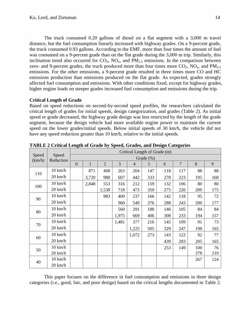
Critical Length of Grade
Based on speed reductions on second-by-second speed profiles, the researchers calculated the
critical length of grades for initial speeds, design categorization, and grades (Table 2). As initial
speed or grade decreased, the highway grade design was less restricted by the length of the grade
segment, because the design vehicle had more available engine power to maintain the current
speed on the lower grades/initial speeds. Below initial speeds of 30 km/h, the vehicle did not
have any speed reduction greater than 10 km/h, relative to the initial speeds.
TABLE 2 Critical Length of Grade by Speed, Grades, and Design Categories
Speed (km/h)
Speed
Reduction
Critical Length of Grade (m)
Grade (%)
0 1 2 3 4 5 6 7 8 9
110 10 km/h 871 408 263 204 147 118 117 88 88
20 km/h 3,720 988 607 442 333 278 223 195 168
100 10 km/h 2,848 553 316 212 159 132 106 80 80
20 km/h 1,538 718 473 350 275 226 200 175
90 10 km/h 983 400 237 166 142 118 95 72
20 km/h 960 549 376 288 243 200 177
80 10 km/h 560 291 188 146 105 84 84
20 km/h 1,975 669 406 308 233 194 157
70 10 km/h 1,481 377 216 145 109 91 73
20 km/h
1,225 505 329 247 198 165
60 10 km/h 1,072 273 143 122 92 77
20 km/h 439 283 205 165
50 10 km/h
253 149 100 76
20 km/h 378 210
40 10 km/h 267 124
20 km/h
This paper focuses on the difference in fuel consumption and emissions in three design
categories (i.e., good, fair, and poor design) based on the critical lengths documented in Table 2.
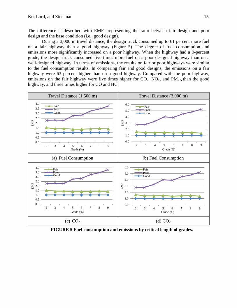
Ko, Lord, and Zietsman 15
The difference is described with EMFs representing the ratio between fair design and poor
design and the base condition (i.e., good design).
During a 3,000 m travel distance, the design truck consumed up to 61 percent more fuel
on a fair highway than a good highway (Figure 5). The degree of fuel consumption and
emissions more significantly increased on a poor highway. When the highway had a 9-percent
grade, the design truck consumed five times more fuel on a poor-designed highway than on a
well-designed highway. In terms of emissions, the results on fair or poor highways were similar
to the fuel consumption results. In comparing fair and good designs, the emissions on a fair
highway were 63 percent higher than on a good highway. Compared with the poor highway,
emissions on the fair highway were five times higher for CO2, NOx, and PM2.5 than the good
highway, and three times higher for CO and HC.
Travel Distance (1,500 m) Travel Distance (3,000 m)
(a) Fuel Consumption (b) Fuel Consumption
(c) CO2 (d) CO2
FIGURE 5 Fuel consumption and emissions by critical length of grades.
0.0
0.5
1.0
1.5
2.0
2.5
3.0
3.5
4.0
2 3 4 5 6 7 8 9
EM
F
Grade (%)
FairPoorGood
0.0
1.0
2.0
3.0
4.0
5.0
6.0
2 3 4 5 6 7 8 9
EM
F
Grade (%)
FairPoorGood
0.0
0.5
1.0
1.5
2.0
2.5
3.0
3.5
4.0
2 3 4 5 6 7 8 9
EM
F
Grade (%)
FairPoorGood
0.0
1.0
2.0
3.0
4.0
5.0
6.0
2 3 4 5 6 7 8 9
EM
F
Grade (%)
FairPoorGood
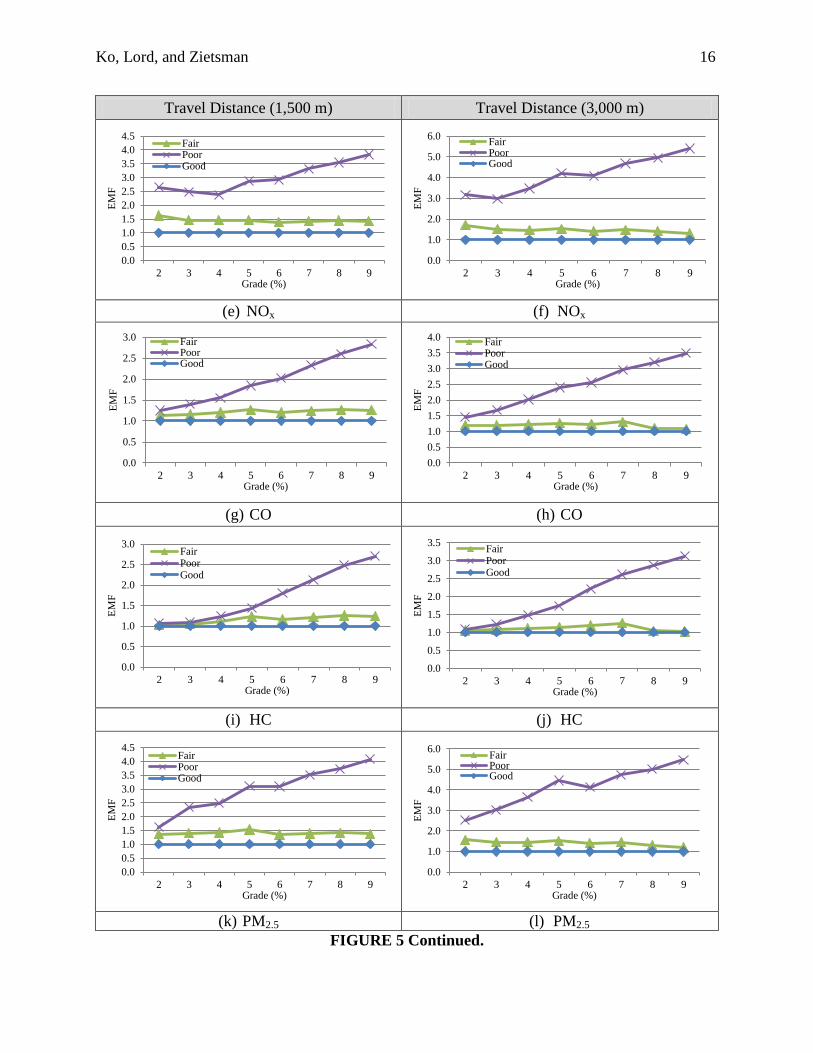
Ko, Lord, and Zietsman 16
Travel Distance (1,500 m) Travel Distance (3,000 m)
(e) NOx (f) NOx
(g) CO (h) CO
(i) HC (j) HC
(k) PM2.5 (l) PM2.5
FIGURE 5 Continued.
0.0
0.5
1.0
1.5
2.0
2.5
3.0
3.5
4.0
4.5
2 3 4 5 6 7 8 9
EM
F
Grade (%)
FairPoorGood
0.0
1.0
2.0
3.0
4.0
5.0
6.0
2 3 4 5 6 7 8 9
EM
F
Grade (%)
FairPoorGood
0.0
0.5
1.0
1.5
2.0
2.5
3.0
2 3 4 5 6 7 8 9
EM
F
Grade (%)
FairPoorGood
0.0
0.5
1.0
1.5
2.0
2.5
3.0
3.5
4.0
2 3 4 5 6 7 8 9
EM
F
Grade (%)
FairPoorGood
0.0
0.5
1.0
1.5
2.0
2.5
3.0
2 3 4 5 6 7 8 9
EM
F
Grade (%)
FairPoorGood
0.0
0.5
1.0
1.5
2.0
2.5
3.0
3.5
2 3 4 5 6 7 8 9
EM
F
Grade (%)
FairPoorGood
0.0
0.5
1.0
1.5
2.0
2.5
3.0
3.5
4.0
4.5
2 3 4 5 6 7 8 9
EM
F
Grade (%)
FairPoorGood
0.0
1.0
2.0
3.0
4.0
5.0
6.0
2 3 4 5 6 7 8 9
EM
F
Grade (%)
FairPoorGood
Ko, Lord, and Zietsman 17
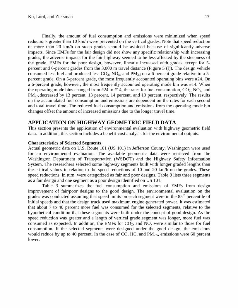
Finally, the amount of fuel consumption and emissions were minimized when speed
reductions greater than 10 km/h were prevented on the vertical grades. Note that speed reduction
of more than 20 km/h on steep grades should be avoided because of significantly adverse
impacts. Since EMFs for the fair design did not show any specific relationship with increasing
grades, the adverse impacts for the fair highway seemed to be less affected by the steepness of
the grade. EMFs for the poor design, however, linearly increased with grades except for 5-
percent and 6-percent grades from the 3,000 m travel distance (Figure 5 (l)). The design vehicle
consumed less fuel and produced less CO2, NOx, and PM2.5 on a 6-percent grade relative to a 5-
percent grade. On a 5-percent grade, the most frequently accounted operating bins were #24. On
a 6-percent grade, however, the most frequently accounted operating mode bin was #14. When
the operating mode bins changed from #24 to #14, the rates for fuel consumption, CO2, NOx, and
PM2.5 decreased by 13 percent, 13 percent, 14 percent, and 19 percent, respectively. The results
on the accumulated fuel consumption and emissions are dependent on the rates for each second
and total travel time. The reduced fuel consumption and emissions from the operating mode bin
changes offset the amount of increased emissions due to the longer travel time.
APPLICATION ON HIGHWAY GEOMETRIC FIELD DATA This section presents the application of environmental evaluation with highway geometric field
data. In addition, this section includes a benefit-cost analysis for the environmental outputs.
Characteristics of Selected Segments
Actual geometric data on U.S. Route 101 (US 101) in Jefferson County, Washington were used
for an environmental evaluation. The available geometric data were retrieved from the
Washington Department of Transportation (WSDOT) and the Highway Safety Information
System. The researchers selected some highway segments built with longer graded lengths than
the critical values in relation to the speed reductions of 10 and 20 km/h on the grades. These
speed reductions, in turn, were categorized as fair and poor designs. Table 3 lists three segments
as a fair design and one segment as a poor design identified on US 101.
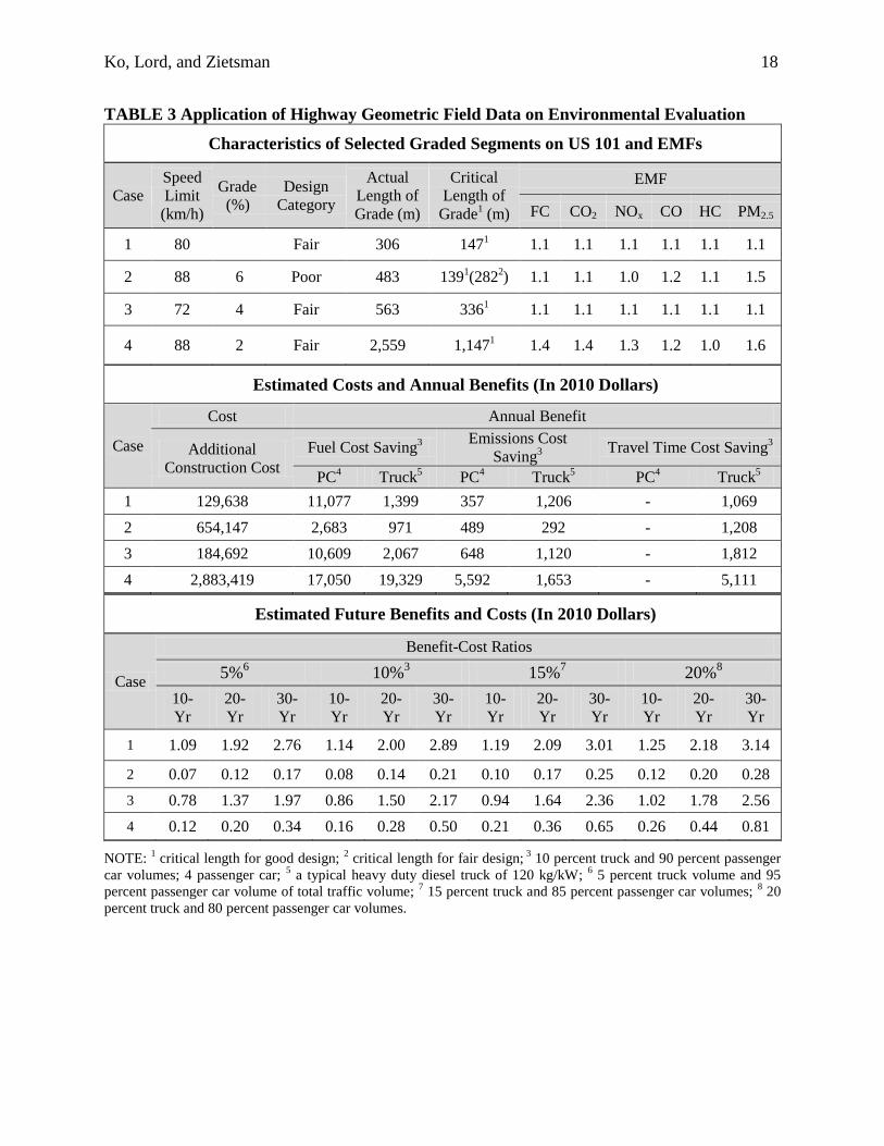
Table 3 summarizes the fuel consumption and emissions of EMFs from design
improvement of fair/poor designs to the good design. The environmental evaluation on the
grades was conducted assuming that speed limits on each segment were in the 85th
percentile of
initial speeds and that the design truck used maximum engine-generated power. It was estimated
that about 7 to 40 percent more fuel was consumed for the selected segments, relative to the
hypothetical condition that these segments were built under the concept of good design. As the
speed reduction was greater and a length of vertical grade segment was longer, more fuel was
consumed as expected. In addition, the EMFs for CO2, and NOx were similar to those for fuel
consumption. If the selected segments were designed under the good design, the emissions
would reduce by up to 40 percent. In the case of CO, HC, and PM2.5, emissions were 60 percent
lower.
Ko, Lord, and Zietsman 18
TABLE 3 Application of Highway Geometric Field Data on Environmental Evaluation
Characteristics of Selected Graded Segments on US 101 and EMFs
Case
Speed
Limit
(km/h)
Grade
(%)
Design
Category
Actual
Length of
Grade (m)
Critical
Length of
Grade1 (m)
EMF
FC CO2 NOx CO HC PM2.5
1 80 6 Fair 306 1471 1.1 1.1 1.1 1.1 1.1 1.1
2 88 6 Poor 483 1391(282
2) 1.1 1.1 1.0 1.2 1.1 1.5
3 72 4 Fair 563 3361 1.1 1.1 1.1 1.1 1.1 1.1
4 88 2 Fair 2,559 1,1471 1.4 1.4 1.3 1.2 1.0 1.6
Estimated Costs and Annual Benefits (In 2010 Dollars)
Case
Cost Annual Benefit
Additional
Construction Cost
Fuel Cost Saving3
Emissions Cost
Saving3
Travel Time Cost Saving3
PC4 Truck
5 PC4 Truck
5 PC4 Truck
5
1 129,638 11,077 1,399 357 1,206 - 1,069
2 654,147 2,683 971 489 292 - 1,208
3 184,692 10,609 2,067 648 1,120 - 1,812
4 2,883,419 17,050 19,329 5,592 1,653 - 5,111
Estimated Future Benefits and Costs (In 2010 Dollars)
Case
Benefit-Cost Ratios
5%6 10%
3 15%
7 20%
8
10-
Yr 20-
Yr 30-
Yr 10-
Yr 20-
Yr 30-
Yr 10-
Yr 20-
Yr 30-
Yr 10-
Yr 20-
Yr 30-
Yr
1 1.09 1.92 2.76 1.14 2.00 2.89 1.19 2.09 3.01 1.25 2.18 3.14
2 0.07 0.12 0.17 0.08 0.14 0.21 0.10 0.17 0.25 0.12 0.20 0.28
3 0.78 1.37 1.97 0.86 1.50 2.17 0.94 1.64 2.36 1.02 1.78 2.56
4 0.12 0.20 0.34 0.16 0.28 0.50 0.21 0.36 0.65 0.26 0.44 0.81
NOTE: 1 critical length for good design;
2 critical length for fair design;
3 10 percent truck and 90 percent passenger
car volumes; 4 passenger car; 5 a typical heavy duty diesel truck of 120 kg/kW;
6 5 percent truck volume and 95
percent passenger car volume of total traffic volume; 7 15 percent truck and 85 percent passenger car volumes;
8 20
percent truck and 80 percent passenger car volumes.
Ko, Lord, and Zietsman 19
Benefit/Cost Analysis The analyses for benefits and costs were applied for the segments listed in Table 3. To perform
an environmental evaluation for the design passenger car, the researchers used the same process
that was applied for the design truck.
A grade adjustment can affect highway construction costs throughout the change of a
lane-length or roadway earthworks. For the selected graded segments (Table 3), the grade design
improvement from fair/poor designs to a good design (i.e., graded to non-graded adjustment on
the section beyond the critical length of vertical grade segment) increased the construction cost
for additional earthwork. However, this grade adjustment did not make any change greater than
one meter in the lane-length at the selected segments. The earthwork volumes were determined
using the average area method under the assumptions that the width of a two-lane highway was 9
m and cut side slopes were 2:1. Additional construction costs for the earthwork were estimated
with the amount of volumes and the unit price (i.e., the price of one cubic meter earthwork was
$9.4 (16)). The costs were about $130,000 to $3 million, depending on the amount of earthwork
needed (Table 3).
Lower vehicle engine loads on the leveled segments resulted in fuel savings. Annual fuel
costs during trips were estimated with fuel consumption per a single passenger car/heavy duty
diesel truck, annual traffic volume, and the unit price of gasoline/diesel. Since WSDOT does not
provide traffic volumes for each type of vehicle, researchers considered various traffic conditions
that showed traffic volumes for the passenger car and the truck accounted for 95 percent and 5
percent, 90 percent and 10 percent, 85 percent and 15 percent, and 80 percent and 20 percent of
annual average daily traffic (AADT), respectively. In 2010, AADTs in the selected cases were
4,600, 1,300, 2,600, and 2,000 vehicles, respectively (17). According to the U.S. Energy
Information Administration (18), in 2010, the average unit prices of gasoline and diesel in
Washington were $2.89 and $2.99, respectively. The fuel costs from the good design condition
were subtracted from those of the fair/poor design condition for both the passenger car and
heavy-duty diesel truck. Under the assumption of a 10-percent truck proportion, the estimated
savings in the fuel cost are provided in Table 3.
Emissions from vehicle movements affect public health and welfare. For example,
children residing close to main roads are at a higher risk of respiratory symptoms (19). Economic
benefits from the emissions reductions were monetized with the unit values of reduced CO2,
NOx, and PM2.5 estimated at $21, $4,000, and $168,000 per metric ton, respectively, in 2007
dollars (20). Each amount of difference in the three emissions resulting from the design
improvement for a single vehicle was multiplied by the annual traffic volume and the unit values
of the emissions per metric ton.
On the roadway vertical grades controlling a speed reduction less than 10 km/h, vehicle
travel times were reduced. In terms of the design truck, there were reductions by up to 11
seconds in travel time on the segments with the good design criteria; however, the design
improvement did not result in travel time savings for the passenger car (130 kW power and 1,478
kg mass), because the car could travel without any speed reduction. Related to the reduced travel
time, the amount of cost savings was estimated under the assumption that the value of the truck
travel time per hour was $22.91 (21).
Benefit/Cost Analysis Results
The benefit-cost analysis was conducted under the assumption of highway operations during 10-
year, 20-year, and 30-year design periods since being built or improved in 2010. In addition,
benefits and costs were adjusted to 2010 dollars with a 3-percent discount rate for societal and
Ko, Lord, and Zietsman 20
health costs and a 7-percent discount rate for fuel and travel time costs (22). For a 10-percent
truck proportion and a 20-year design period, the benefits surpassed the costs in half of the cases
(Table 3). As described in Case 1, the cost savings from the design improvement was two times
greater than the construction cost of the additional earthwork for a 20-year design period.
However, for half of the selected cases, the design improvements were not beneficial for a 30-
year design period due to a significant amount of additional construction costs. In terms of truck
proportions, the cost/benefit ratios increased with higher truck proportions.
DISCUSSION AND CONCLUSIONS This paper has presented guidelines and tools on environmental impacts for quantifying fuel
consumption and emissions for the design of vertical grades. These guidelines and tools play an
important role in reducing the uncertainty in engineering judgment for environmentally-friendly
highway grade design. The research shows that adverse environmental impacts from vehicle
movements on vertical grades can be controlled and reduced throughout environmentally-
conscious highway design.
When traveling at an initial speed lower than a crawl speed, the truck could accelerate up
to the crawl speed due to available tractive force. However, the truck decelerated to the crawl
speed due to grade resistance forces when starting with an initial speed higher than the crawl
speed. The positive impact of high speeds on VSPs was neutralized by the negative impact of
deceleration on VSPs. In addition, shorter travel times resulting from higher initial speeds
assisted in saving fuel and reducing emissions during the trip. At least 26 percent of the fuel
costs and emissions could be saved by starting the trip with an initial speed of 110 km/h relative
to 10 km/h on the vertical grades lengthened to 1,500 m and 3,000 m. Faster initial speeds in the
grade design would help in reducing fuel consumption and emissions (which the highway
designer cannot control).
For the grade variable, the impact was more distinctive. Steeper grades caused more
speed reductions and increased travel times on the vertical grade segments. Fuel consumption
and emissions increased by a factor of up to four on a 9-percent graded segment compared to a
leveled segment. Steeper grades caused more fuel to be consumed and emissions produced due
to high vehicle engine loads and longer travel times. The Green Book specifies that most
passenger cars can travel on graded highways as steep as 4 to 5 percent without a significant
speed reduction (1). However, it is clear that steep grades have adverse environmental impacts
on the vehicle movement.
For the critical length, the concept of design categories of good, fair, and poor were used.
When the fair design criteria was applied for the vertical grade design, the fuel consumption and
emissions increased because of extended travel time resulting from the speed reduction; the
design vehicle consumed fuel and produced emissions up to 70 percent more in the fair design
than with the good design. The poor design criteria had even more adverse results. The fuel
consumption and emissions with the poor design increased by a factor of up to five relative to the
good design criteria. This was due to significantly longer travel times. Good grade design
preventing significant speed reduction not only improved highway safety but also reduced the
degree of adverse environmental impacts.
The data collected in Washington State showed that the design truck consumed up to 35
percent more fuel and produced up to 61 percent more emissions on the actual grades, relative to
the hypothetical condition that these segments were built under the concept of controlling speed
reduction of less than 10 km/h. The benefit/cost analysis showed that the economic benefits
Ko, Lord, and Zietsman 21
exceeded the costs for half of the segments for a 20-year design period. The design improvement
could lead to reductions in direct, indirect, and societal costs related to vehicle fuel, societal and
public health, and travel time; the monetary savings surpassed the construction costs resulting
from additional earthwork. However, the design improvements on the other half of the segments
were not beneficial for the design period because of the additional construction costs caused by
the unbalanced cut and fill volumes. In addition, it should be pointed out that the results are
dependent on the assumptions related to the selection of the design vehicle characteristics, fuel
type, weather conditions, traffic condition, and/or truck proportion of total traffic volume. The
results should not be taken at face-value and should not be used for decision-making purposes. In
addition, additional fuel consumption and emissions due to the construction for the flattening
grade were not considered in the benefit-cost analysis. As future research, a systematic tool
predicting fuel consumption and emissions based on various design and traffic conditions will be
beneficial; highway designers and engineers can predict the environmental impact based on the
selected conditions and compare that impact with other conditions without any complex
calculation and repetitive processing used in this study. In addition, validation of the findings at
this research with real-world drive-cycles and measurements is an important topic for future
research.
REFERENCES 1. AASHTO. A Policy on Geometric Design of Highways and Streets (6th Edition). American
Association of State and Highway Transportation Officials, Washington, D.C., 2011.
2. AASHTO. Highway Safety Manual. American Association of State and Highway
Transportation Officials, Washington, D.C., 2010.
3. Ko, M. Incorporating Vehicle Emission Models into the Highway Design Process. Ph.D.
Dissertation, Zachry Department of Civil Engineering, Texas A&M University, College
Station, Texas, 2011.
4. Ko, M., D. Lord, and Z. Zietsman. Environmental conscious highway design for vertical
crest curves. In Transportation Research Record: Journal of the Transportation Research
Board, No. 2270, Transportation Research Board of the National Academies, Washington, D.
C., 2012, pp. 96-106.
5. Servin, O., K. Boriboonsomsin, and M. Barth. An Energy and Emission Impact Evaluation of
Intelligent Speed Adaptation. The IEEE ITSC, 2006.
6. Song, G., and L. Yu. Estimation of Fuel Efficiency of Road Traffic by Characterization of
Vehicle-Specific Power and Speed Based on Floating Car Data. In Transportation Research
Record: Journal of the Transportation Research Board, No. 2139, Transportation Research
Board of the National Academies, Washington, D. C., 2009, pp. 11-20.
7. Qi, Y. G., H. H. Teng, and L. Yu. Microscale Emission Models Incorporating Acceleration
and Deceleration. Journal of Transportation Engineering, Vol. 130, No. 3, 2004, pp. 348-
359.
Ko, Lord, and Zietsman 22
8. Ahn, K., H. Rakha, A. Trani, and M. Van Aerde. Estimating Vehicle Fuel Consumption and
Emissions Based on Instantaneous Speed and Acceleration Levels. Journal of Transportation
Engineering, Vol. 128, No. 2, 2002, pp. 182-190.
9. Boriboonsomsin, K., and M. Barth. Impacts of Road Grade on Fuel Consumption and Carbon
Dioxide Emissions Evidenced by Use of Advanced Navigation Systems. In Transportation
Research Record: Journal of the Transportation Research Board, No. 2139, Transportation
Research Board of the National Academies, Washington, D. C., 2009, pp. 21-30.
10. Rakha, H., L. Lucic, S. H. Demarchi, J. R. Setti, and M. Van Aerde. Vehicle dynamics model
for predicting maximum truck acceleration levels. Journal of Transportation Engineering,
Vol. 127, No. 5, 2001, pp. 418-425.
11. Mannering, F. L., S. S. Washburn, and W. P. Kilareski. Principles of Highway Engineering
and Traffic Analysis. Hoboken: John Wiley & Sons, Inc., 2009.
12. Lan, C.-J. and M. Menendez. Truck speed profile models for critical length of grade. Journal
of Transportation Engineering, Vol. 129, No. 4, 2003, pp. 408-419.
13. Bester, C. J. Truck speed profiles. In Transportation Research Record: Journal of the
Transportation Research Board, No. 1701, Transportation Research Board of the National
Academies, Washington, D. C., 2000, pp. 110-115.
14. EPA, 2010. User Guide for MOVES2010a. Report No. EPA-420-B-10-036, EPA,
Washington, D.C. Retrieved October 2010 from http://www.epa.gov/oms/models
/moves/movesback.htm.
15. Lamm, R., B. Psarianos, T. Mailaender, M. Choueiri, R. Heger, and R. Steyer. Highway
Design and Traffic Safety Engineering Handbook. New York: McGraw-Hill, 1999.
16. Washington Department of Transportation (WSDOT), 2011a. WSDOT Construction Cost
Trend. http://www.wsdot.wa.gov/biz/construction/constructioncosts.cfm, accessed July 12,
2011.
17. Washington Department of Transportation (WSDOT), 2011b. 2010 Annual Traffic Report.
http://www.wsdot.wa.gov/mapsdata/travel/pdf/Annual_Traffic_Report_2010.pdf, accessed
June 21, 2011.
18. U.S. Department of Energy, 2011. Departmental Guidance for the Valuation of Travel Time
in Economic Analysis. Washington, D. C. http://ostpxweb.dot.gov/policy/Data/VOT
revision1_2-11-03.pdf, accessed May 21, 2011.
19. Middleton, N., P. Yiallouros, N. Nicolaou, S. Kleanthous, S. Pipis, M. Zeniou, P.
Demokritou, and P. Koutrakis. Residential exposure to motor vehicle emissions and the risk
of wheezing among 7-8 year-old schoolchildren: a city-wide cross-sectional study in Nicosia,
Cyprus. Environmental Health, Vol. 9, No. 28, 2010.
Ko, Lord, and Zietsman 23
20. Burris, M. Seattle/LWC Urban Partnership Agreement National Evaluation: Cost Benefit
Analysis Test Plan. Texas Transportation Institute, 2011.
21. U.S. Department of Transportation, 2003. Transportation Energy Data Book. Washington,
D. C. http://cta.ornl.gov/data/chapter1.shtml, accessed November 1, 2011.
22. NHTSA. Final Regulatory Impact Analysis: Corporate Average Fuel Economy for MY 2011
Passenger Cars and Light Trucks. Office of Regulatory, Analysis and Evaluation, National
Center for Statistics and Analysis, National Highway Transportation Safety Administration,
2009.