EPA Hydraulic Fracturing WorkshopMarch 10th - 11th, 2011

2

“Fracture Design in HorizontalShale Wells – Data Gathering

to Implementation”

Tim BeardSr. Engineering Advisor - Completions

Chesapeake Energy Corporation6100 N. Western Avenue ı Oklahoma City, OK 76118 ı 405-935-8000

AskChesapeake@chk.com ı chk.com ı NYSE: CHK

3

Goal

Planning

• Data

• Measuring

Validating•

• Properties Needed in Modeling

• Designing the Hydraulic Fracture

• Frac Models in Vertically

Heterogeneous Formations

Execution

Presentation Overview

4

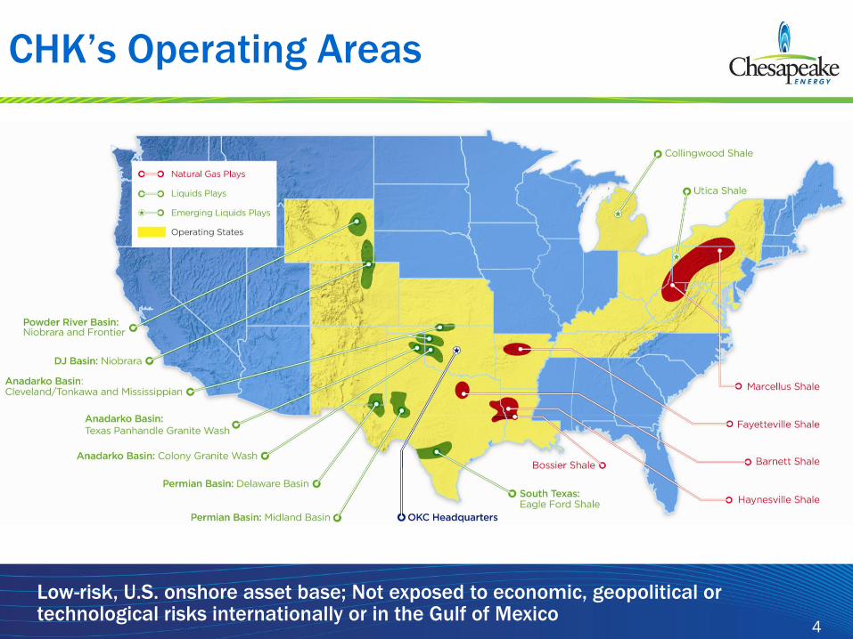
CHK’s Operating Areas

Low-risk, U.S. onshore asset base; Not exposed to economic, geopolitical or technological risks internationally or in the Gulf of Mexico

Shale Information

Shale Play Fayetteville Barnett Eagle Ford Haynesville Marcellus

Average Depth From

Surface (ft)

4,500 7,400 9,000 11,500 7,100

Bottom Hole

Temperature (F)

130 190 260 320 145

Bottom Hole

Pressure (psi)

2,000 2,900 6,200 10,000 4,600

5

6

What is the Goal of Hydraulic Fracturing?

Maximize the Stimulated Reservoir Volume (SRV)

along the horizontal wellbore for a given well

spacing to maximize hydrocarbon production within

the zone of interest.

Orientation and lateral length

Vertical placement within flow unit

Rock Properties/Mechanics

Stages/Perf Clusters/Isolation

Fluid and proppant selection

7

Planning

8

What data do we use?

What are the main variables that need

to be factored into each frac design?

• Porosity and Permeability

Lateral Length

Brittleness vs. Ductility

•

•

• Young’s Modulus

Poisson’s Ratio

Fracture Toughness

•

•

• Thickness

Barriers

Depth

In-Situ Stress

•

•

•

• Maximum Principle

Stress Direction

• Lithology of Pay

Stress Anisotropy

Natural Fractures

Gas or Liquids Reservoir

Temperature

Reservoir Pressure

•

•

•

•

•

9

Wireline Log Data

Logs are run in regionally representative pilot wells over the

zone(s) of interest.

Triple Combo Log, Spectral Gamma Ray, Dipole Sonic Log, Formation

MicroImager

The data gathered from the logs is utilized to do a

petrophysical analysis and to calculate the rock mechanical

properties of the reservoir to determine pay intervals, barriers,

etc.

FMI and multi-caliper log data are also used to determine a

maximum and minimum principle stress direction and to

determine if there are natural fractures present.

10

Lateral Orientation

Maximum Principle Stress Direction

Lateral Placement

● Perpendicular to maximum principle stress

Optimize transverse fracturing

Slight variations for more efficient pattern

development

●

●

11

Well: PROCKO_MARTIN_WHITMAN_625599

DATE PLOTTED: 27-Oct-2008

HORIZONTAL UNITS: FEET

Y COORDINATE: 14416529.67

X COORDINATE: 1745180.06

LONGITUDE: 80.0000

LATITUDE: 39.0000

LOCATION: TWP - Range - Sec

COMPANY: CHK

VERTICAL SCALE: 1:240

DATE LOGGED: 31-Jul-2007

VERTICAL UNITS: FEET

DRILLED DEPTH: 7780.00

ELEVATION MEAS. REF.: -

MEASUREMENT REF.:

SURFACE ELEVATION: 15.00

DATUM FOR ELEVATION: GR

RM

- @ -

RMC

- @ -

RMF

- @ -

DFD

-

BHTDEPTH (FEET)

7120.00-7429.00

SHT BIT SIZE

Composite

- --

bsIN6 16

HCAL_1IN4 24

DCAL_1IN0 10

TOTAL_GAMMA_1GAPI0 200

GR_1GAPI0 200

HDRA_1G/C30.75 -0.25

7150

7200

7250

7300

7350

7400

7120.0

7429.0

DEPTHFEET

209.0

RE

SE

RV

OIR

_IN

T.N

ET

PE

RF

S.P

ER

FS

TR

EA

TM

EN

T.S

TA

GE

RXO8_1OHMM0.2 2000

RLA2_1OHMM0.2 2000

RLA3_1OHMM0.2 2000

RLA4_1OHMM0.2 2000

RLA5_1OHMM0.2 2000

TENS_1LBF10000 3000

45678910111213141516

17181920212223242526272829

30313233343536

37383940

4142

43444546

474849

50515253545556

57585960616263

6465666768697071

72737475

7677

7879808182

8384

8586

878889909192

93949596979899100101102

103104105

106107

108109110111

112113114115116117118119120121122123124

125126127128129130131132133

134135136137138139140141142143144

145146147148149150151

152153154

CO

RE

_T

RA

.SA

MP

LE

_ID

NPHI_1V/V0.3 -0.1

NPHI_N_3MV0.3 -0.1

RHOZ_1G/C32.18 2.88

RHOBC_4G/C32.18 2.88

CDEN_1G/C32.18 2.88

crhobFEET2.18 2.88

PEFZ_1B/E10 0

2.55

RE

SE

RV

OIR

_IN

T.R

HO

BC

_A

M

BVH_3V/V0.2 0

BVH_RHOB_TRS_3V/V0.2 0

PHIE_3V/V0.2 0

vol_tocV/V0 0.4

VOL_TOC_3V/V0 0.4

VP_TOC_1V/V0 0.4

VP_TOC_2V/V0 40

pignV/V0.2 0

CPHI_1V/V20 0

CPHI_GAS_1V/V20 0

0.060

RE

SE

RV

OIR

_IN

T.V

OL

_T

OC

_A

M

0.056

RE

SE

RV

OIR

_IN

T.B

VH

_A

V

VCLAY_3V/V0 1

vcl_grlimV/V0 1

VP_VCLAY_1V/V0 100

0.429

RE

SE

RV

OIR

_IN

T.V

CL

AY

_A

M

SW_3V/V1 0

CSW_1V/V100 0

suwiV/V1 0

CSO_1F/MN0 100

0.127

RE

SE

RV

OIR

_IN

T.S

W_

AV

CPERM_1V/V1.e-06 1

CPERM_12_20_1V/V1.e-06 1

CPERM_COMPOSITE_1V/V1.e-06 1

cpermV/V1.e-06 1

CKPERM_3B/E1.e-06 1

PERM_DENONLY_1MM2/MS1.e-06 1

KH_PRO_1

B/E1.e-06 1

kintxMD1.e-06 1

T_FLOW UNIT

T_ONONDAGA

T_HUNTERSVILLE

PETRO.FORMATIONPERFS.COMPLETION

0.1012

RE

SE

RV

OIR

_IN

T.C

KP

ER

MH

0.000484

RE

SE

RV

OIR

_IN

T.C

KP

ER

M_

AM

●

●

●

Lateral Placement

Target highest quality rock with

consideration given to stress profile

and fracture geometries

Preferred lateral placement in upper to

middle portion of target zone to

optimize proppant placement

Toe high with option of traversing the

entire section

12

Mechanical Properties and StressEstimation from Acoustic Logs

Elastic Moduli Estimated from Acoustic

Logs

Several Stress Equations are Appropriate

Uniaxial Transverse Isotropic Equation

(Lateral Strain Model):

σHmin = (Eh/Ev)(νv/(1-νh))(σv-αPp) +

αPp + (Eh/(1-vh2))εhmin + (Ehvh/(1-

vh2))εhmax

This equation expands the σtectonic to

incorporate lateral strain. Tectonic strain

creates greater stress in stiff

sandstone/limestone beds and less

stress in organic-rich shales.

Estimated Stress Calibrated with Well

Test

13

Pump-In Testing: Key Calibration

Pump-In Tests

Conventional Pump-In Tests in Cased Hole

― Closure Stress is Determined

After Closure Analysis―

MDT Pump-In Tests in Open Hole

― Closure Stress is Determined

Core Data

The pump-in tests along with the core

data calibrate mechanical properties

data.

14

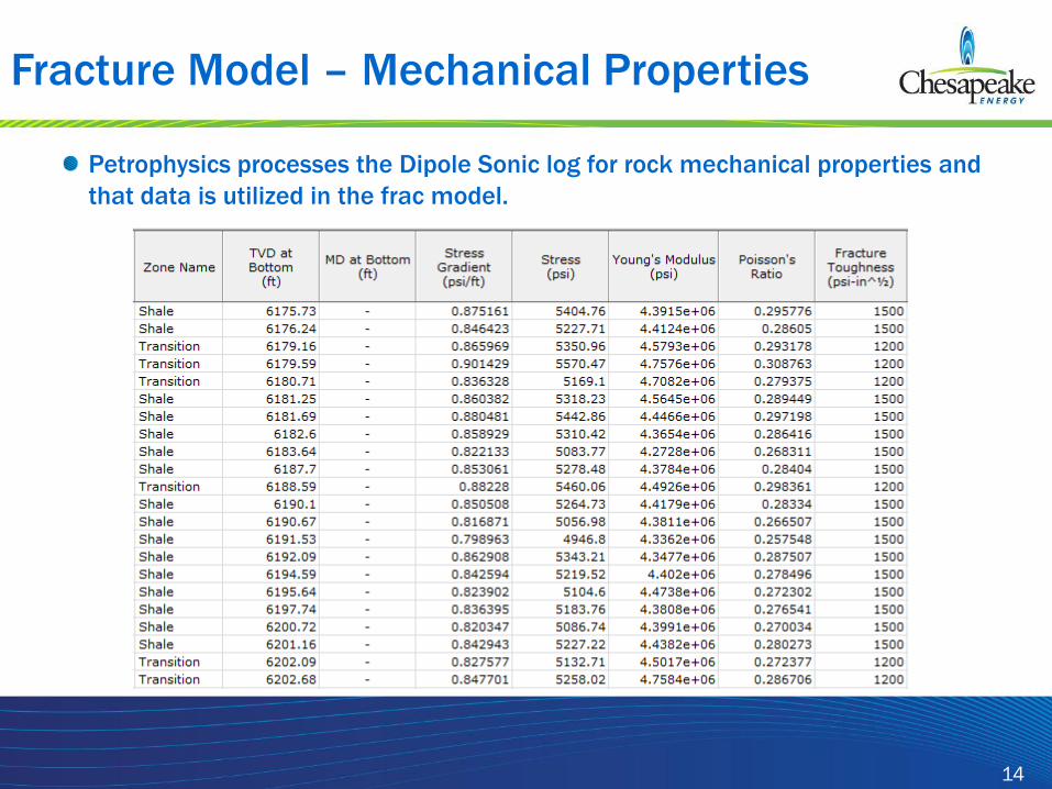
Fracture Model – Mechanical Properties

Petrophysics processes the Dipole Sonic log for rock mechanical properties and

that data is utilized in the frac model.

15

Fracture Model – Fluid Flow and Leakoff

The fluid loss data input into the model.

16

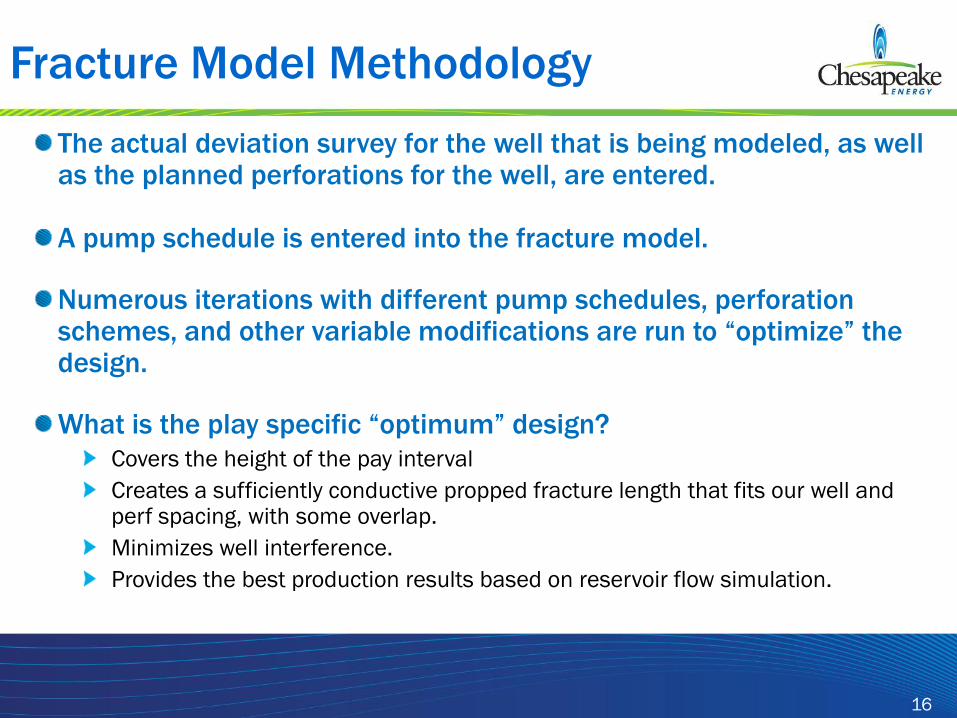
Fracture Model Methodology

The actual deviation survey for the well that is being modeled, as well as the planned perforations for the well, are entered.

A pump schedule is entered into the fracture model.

Numerous iterations with different pump schedules, perforation schemes, and other variable modifications are run to “optimize” the design.

What is the play specific “optimum” design?

Covers the height of the pay interval

Creates a sufficiently conductive propped fracture length that fits our well and perf spacing, with some overlap.

Minimizes well interference.

Provides the best production results based on reservoir flow simulation.

17

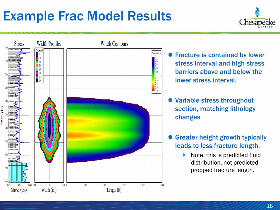
Example Frac Model Results

As depicted in the model, the

fracture propogates primarily only

in the lower stress portion of the

rock.

The lower stress portion of the

reservoir “contains” the frac

High stress barriers exist above

and below the fracture matching

lithology changes.

Vertical variations in stress exist

throughout the sections depicted.

18

Example Frac Model Results

Fracture is contained by lower

stress interval and high stress

barriers above and below the

lower stress interval.

Variable stress throughout

section, matching lithology

changes

Greater height growth typically

leads to less fracture length.

Note, this is predicted fluid

distribution, not predicted

propped fracture length.

19

Perforation Clusters and Stage Spacing

250 ’– 500’ Stage Spacing

50 ’– 100’ Cluster Spacing

Not To Scale

20

Fluid Selection

Utilize core data and lab fluid-rock sensitivity testing to

determine fluid additives

Maximize slickwater volumes vs. gelled fluid volumes

Utilize light gels/crosslink to place higher sand

concentrations where necessary in gas shales

In liquids rich plays, more gels or crosslinked gels are

utilized to promote greater conductivity in the propped

fractures

Reservoir modeling suggests higher primary fracture

conductivity required to improve well performance

CHK Promotes development and leads in the use of

“greener”, more environmentally friendly hydraulic

fracturing additives

21

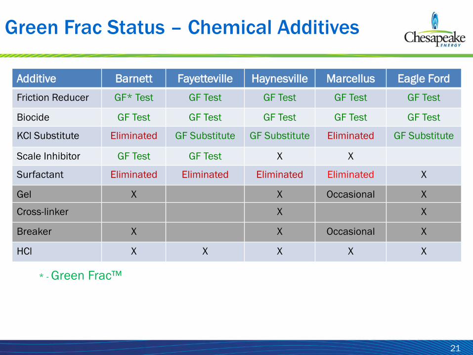
Green Frac Status – Chemical Additives

Additive Barnett Fayetteville Haynesville Marcellus Eagle Ford

Friction Reducer GF* Test GF Test GF Test GF Test GF Test

Biocide GF Test GF Test GF Test GF Test GF Test

KCl Substitute Eliminated GF Substitute GF Substitute Eliminated GF Substitute

Scale Inhibitor GF Test GF Test X X

Surfactant Eliminated Eliminated Eliminated Eliminated X

Gel X X Occasional X

Cross-linker X X

Breaker X X Occasional X

HCl X X X X X

* - Green Frac™

22

Proppant Selection

100 mesh sand is typically used in the early portion of

the job for enhanced distance and height, diversion,

etching, and as a propping agent

40/70 and 40/80 mesh proppants are currently the

predominant proppants used in gas shales

30/50 and 20/40 proppant used in some areas for

fracture conductivity enhancement (especially important

in the liquids rich plays)

Resin Coated Tail-Ins - used where sand flowback is an

issue or where more proppant strength and conductivity

are needed

Ceramic Proppants are utilized where higher conductivity

and higher strength are required

Increased proppant volumes and less fluid addresses

conductivity and environmental issues

23

Execution

24

•

Typical Hydraulic Fracturing Job:

10-20 Pumps

2-4 Sand Storage Units

Blender

Hydration Unit

Frac Tanks

Chemical Storage Truck

Data Monitoring Van

20-30 Workers

Hydraulically Fracturing the Shale

•

•

•

•

•

•

•

25

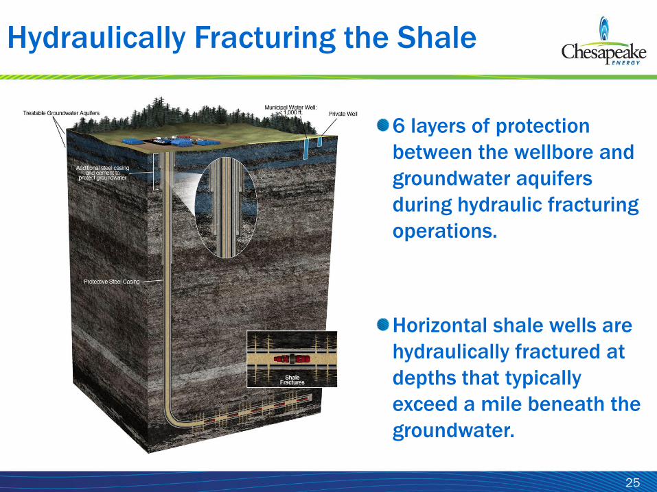
Horizontal shale wells are

hydraulically fractured at

depths that typically

exceed a mile beneath the

groundwater.

6 layers of protection

between the wellbore and

groundwater aquifers

during hydraulic fracturing

operations.

Hydraulically Fracturing the Shale

26

Summary

Planning and executing an “optimum” hydraulic

fracture requires a multidisciplinary approach of

gathering data, confirming data, modeling the

optimum fracture and well performance, and

executing a plan based on those models.

Hydraulic Fracture models do a good job of

depicting and/or predicting vertical barriers and

thus fracture growth.

This data has been, and continues to be, confirmed

in multiple ways.

― Microseismic

Lab Tests

Core Data

―

―

27

Summary

Extensive data collection results in

hydraulic fracturing jobs that are

designed to remain in the proper

formation

Remaining in the zone of interest

maximizes production and minimizes

opportunities to negatively impact

production

Hydraulic fracturing is a highly

engineered process that takes into

account numerous variables.

28

Thank You – Questions?

Tim BeardSr. Engineering Advisor - Completions

Chesapeake Energy Corporation6100 N. Western Avenue ı Oklahoma City, OK 76118 ı 405-935-8000

AskChesapeake@chk.com ı chk.com ı NYSE: CHK

Fracture Design in Horizontal Shale Wells – Data Gathering to Implementation

Tim Beard Chesapeake Energy Corporation

The statements made during the workshop do not represent the views or opinions of EPA. The

claims made by participants have not been verified or endorsed by EPA.

Introduction

Hydraulic fracturing has been used in the petroleum industry since the late 1940s. However, the hydraulic fracturing of horizontal shale wells is a relatively new practice. Although relatively “new,” the hydraulic fracturing of horizontal wells is still governed by the same physics as a conventional reservoir. The biggest differences between hydraulic fracturing operations in a more conventional and shale reservoir are the type of fluids utilized and the volume of fluid and sand pumped. The increase in fluid and sand volume in shale wells is primarily due to the need to maximize stimulated reservoir volume (SRV) in the relatively low permeability formation. The goal of hydraulically fracturing a typical shale play is to contact as much of the reservoir rock as possible with proppant-filled fractures. The total volume contained between all propped fractures along the wellbore represents the SRV. To maximize the SRV, there are many variables that must be considered prior to drilling a horizontal shale well. This abstract will focus on general fracture design in horizontal shale plays across the U.S. with an emphasis on the data taken into consideration for each frac job and a brief discussion of how that data is obtained and used. Additional discussion will be focused on frac modeling and the validity of frac barriers. Finally, a brief discussion of the diagnostics used to determine frac placement will be included.

Planning to Hydraulically Fracture a Horizontal Shale Well

Prior to drilling, companies must gather local and regional in-situ stress data (usually by drilling a pilot hole and running logs), and make economic and land decisions concerning the orientation, length, and placement of the lateral prior to drilling a horizontal well. With the obtained stress data and reservoir properties, evaluation and design of the horizontal well and stimulation is performed comprising some of the key analyses and tasks briefly described below.

Orientation and Lateral Length

One of the first variables that is considered when drilling a horizontal shale well is the maximum and minimum principle stress orientation in the target formation. These data are typically estimated from wireline logs in a pilot hole. The maximum and minimum principle stress directions are typically consistent throughout a given geographic area. Therefore, a few

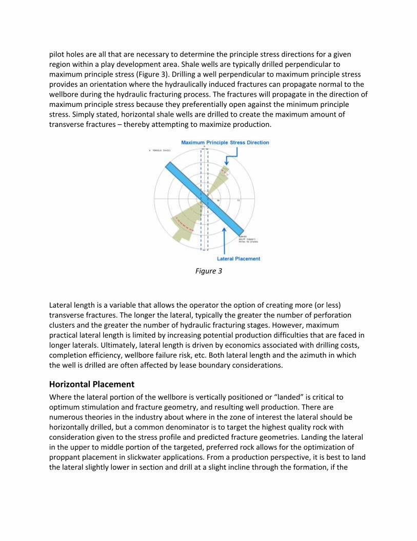
pilot holes are all that are necessary to determine the principle stress directions for a given region within a play development area. Shale wells are typically drilled perpendicular to maximum principle stress (Figure 3). Drilling a well perpendicular to maximum principle stress provides an orientation where the hydraulically induced fractures can propagate normal to the wellbore during the hydraulic fracturing process. The fractures will propagate in the direction of maximum principle stress because they preferentially open against the minimum principle stress. Simply stated, horizontal shale wells are drilled to create the maximum amount of transverse fractures – thereby attempting to maximize production.

Figure 3

Lateral length is a variable that allows the operator the option of creating more (or less) transverse fractures. The longer the lateral, typically the greater the number of perforation clusters and the greater the number of hydraulic fracturing stages. However, maximum practical lateral length is limited by increasing potential production difficulties that are faced in longer laterals. Ultimately, lateral length is driven by economics associated with drilling costs, completion efficiency, wellbore failure risk, etc. Both lateral length and the azimuth in which the well is drilled are often affected by lease boundary considerations.

Horizontal Placement

Where the lateral portion of the wellbore is vertically positioned or “landed” is critical to optimum stimulation and fracture geometry, and resulting well production. There are numerous theories in the industry about where in the zone of interest the lateral should be horizontally drilled, but a common denominator is to target the highest quality rock with consideration given to the stress profile and predicted fracture geometries. Landing the lateral in the upper to middle portion of the targeted, preferred rock allows for the optimization of proppant placement in slickwater applications. From a production perspective, it is best to land the lateral slightly lower in section and drill at a slight incline through the formation, if the

formation dip allows for this approach. This “toe up” drilling practice promotes less liquid hold-up or build-up across the lateral.

Data Gathering

Once the lateral is drilled, the planning of the actual hydraulic fracturing takes into account many variables obtained from data gathered in each wellbore (or in pilot holes) by logging, and in some cases, analysis of core samples. Some, but not all, of the variables that are involved in the fracture design include:

• Porosity and Permeability • Brittleness vs. Ductility

• Young’s Modulus • Poisson’s Ratio

• Thickness • Barriers • Depth • In-Situ Stress • Lithology • Stress Anisotropy • Natural Fractures • Gas or Liquids Reservoir • Temperature • Reservoir Pressure

Young’s Modulus and Poisson’s ratio are typically calculated from the shear and compressional data estimated from dipole-sonic log response. These values are then used to calculate the in-situ stress of the rock using several possible stress equations. A stress equation that is applicable in many transverse isotropic shales plays is:

σHmin = (Eh/Ev)(νv/(1-νh))(σv-αPp) + αPp + (Eh/(1-vh2))εhmin + (Ehvh/(1-vh

2))εhmax

Where: σHmin = Minimum Horizontal Stress

Eh = Horizontal Young’s Modulus Ev = Vertical Young’s Modulus νv = Vertical Poisson’s Ratio νh = Horizontal Poisson’s Ratio σv = Vertical Stress α = Biot’s Coefficient Pp = Pore Pressure εhmin = Minimum Horizontal Strain εhmax = Maximum Horizontal Strain

This equation recognizes that shales are anisotropic. With lower νh in organic rich shales and greater Eh, the difference in σHmin between shale and sandstone/limestone decreases and often reverses. This leads to a minimum stress in shales and the bounding sandstone/limestone become barriers. The equation above has also replaced the stectonic term that has been used in the past, to incorporate lateral strain ((Eh/(1-vh

2))εhmin + (Ehvh/(1-vh2))εhmax). For stiff

sandstone/limestone interbedded with slightly less stiff shale, the tectonic strain creates greater stress in the stiffer beds and less stress in the shales. This equation is the best fit for pump-in data in the field.

Data Verification and Calibration

Pump-in tests are done on regionally representative wells to obtain actual stress values and validate estimated stresses obtained from the above equation. A typical pump-in test is done by pumping into a well at a rate high enough to fracture the rock with a small volume of fluid, followed by a time period of hours to measure closure. This closure pressure provides the actual σHmin. After-closure analysis can also be performed by observing a well post-closure to determine permeability, pore pressure, etc. Core data are also a valuable tool in elastic properties measurement and calibration of wireline-interpreted elastic moduli.

Fracture Modeling

Estimation of fracture geometry is modeled using an analytical fracture modeling simulator. Rock mechanical properties and fluid loss data (permeability, porosity, pressure, compressibility, fracturing fluid properties, etc.) are principal inputs into fracture modeling. After entering the directional survey of the wellbore, an iterative process of comparing and contrasting models using differing variables is performed with the goal of designing the “optimum” hydraulic fracture for the given set of reservoir properties. An “optimum” fracture design is one that:

1) Fractures the height of the pay interval 2) Creates a sufficiently conductive propped fracture half length that fits the well and

perforation cluster spacing, with some overlap. 3) Minimizes well interference 4) Takes into consideration the numerous variables, and accounts for the role played by

each parameter to achieve the largest SRV and ultimately the greatest production.

Fracture length and height are two primary outputs of fracture modeling software. The example model (Figure 4) below shows a fracture half length of ~1,200’ and a fracture height of ~100’. As can be seen, the fracture is contained in a lower stress region of the overall stress column. Barriers exist above and below the primary zone of interest, confining the fracture to the lower stress interval.

Figure 4

The model below (Figure 5) also shows a fracture that is contained by a lower stress interval with higher stress intervals above and beneath. It can be seen that the fracture half length is ~800’ and the fracture height is ~250’. A number of factors control the height growth of a fracture, but the relative difference between the stresses in and around the fracture is the most important factor. Fractures tend to remain in low stress vertical regions that effectively “lock in” or “trap” the fracture and keep it from breaking into higher stress rock. Staying in the reservoir rock is highly desired because remaining in the zone of interest maximizes the operators production and minimizes the wasting of frac energy on non-productive rock.

Figure 5

Perforation Clusters and Stage Spacing

The number of perforation clusters per stage and the spacing of the clusters are area and shale specific. In the majority of shale plays the perforation clusters are 50-100’ apart. This spacing of perforation clusters is very dependent on a number of variables. More permeability and porosity typically allows for greater spacing between clusters. The greater the number of natural fractures, typically the greater the spacing between clusters. A lower stress anisotropy (which typically leads to greater frac complexity), typically results in a greater distance between clusters. In more ductile shales, the distance between perforation clusters will be shortened. Similarly, in a hydrocarbon liquids-rich play, where greater conductivity is typically desired, the distance between perforation clusters will be shortened. Stage spacing typically correlates with perforation cluster spacing. In the majority of the shale plays 4-6 perforation cluster per stage is normal. The greater the number of perforation clusters, the less likely it is that each cluster will get adequately treated. Thus, limiting the number of clusters per stage typically leads to more stimulated reservoir volume. A typical stage length is 250–500 ft.

Fluid Selection

Many variables are involved in fracture fluid chemistry design (i.e., brittleness vs. ductility, highly anisotropic vs. low anisotropy, rate that can be achieved, fluid-rock sensitivity, etc.). Prior to pumping any fluid systems, fluid-rock core measurements are used to determine the fluid additives necessary in each play to prevent formation damage from drilling or fracture fluids. The majority of the shale plays in North America are treated with a large percentage of “slickwater”. Slickwater is predominantly fresh water with additives (typically ~11 chemical additives) that constitute less than 1 percent by volume of the liquid pumped. Slickwater is frequently the fracture fluid of choice due to the lack of damage to the formation and its ability to increase fracture complexity within the shales, as compared to more viscous linear or crosslinked gels. Light gels are often used at the end of a stage to transport higher sand concentrations. In hydrocarbon liquids-rich plays, more gels are typically utilized to carry higher concentrations of coarser-grained proppant, allowing greater fracture conductivity. Based on the nature of the induced fracture geometries, the volumes of fluids pumped, and the position of fractured intervals within the geologic column, Chesapeake Energy, the American Petroleum Institute and the American Natural Gas Alliance estimate that the risk of contamination to groundwater from hydraulic fracture stimulation of deep shale unconventional gas is extremely small to non-existent in most settings. However, we do realize that there are employees who routinely work around hydraulic fracturing additives and while safety is paramount in our industry, there is always the potential for an accidental surface spill. It was with the concern for our employees and the potential for spills in mind that we forged our “Green Frac” program. Chesapeake Energy’s Green Frac™ program was initiated in 2009 to determine if it was possible to improve the overall environmental “footprint” of the additives used in our hydraulic

fracturing operations. A primary goal was to eliminate any additive that was not absolutely critical to successful completion and operation of our wells. For those deemed critical, materials have been selected that pose lower risk to personnel and to the environment in the event of an accidental surface discharge. To date, we have either eliminated, have found more desirable substitutes, or are in the process of successfully testing substitutes for the majority of additives historically used in hydraulic fracturing of unconventional shales.

Proppant Selection

Proppant selection is based on such factors as; the particular stresses to which the proppants will be subjected, the amount of fracture flow conductivity required, propped fracture length designed, and complexity estimated. Different proppants fit different plays and wells within plays. A 100-mesh sand is frequently used in the early portion of many hydraulic fracturing stages for diversion, etching, and as a propping agent. Larger 40/70- and 40/80-mesh proppants are presently the predominant proppants used in gas shales. Still larger 30/50- and 20/40-mesh proppants are used in some areas for conductivity enhancement. The larger proppants are especially important in liquids-rich environments. Resin-coated proppants are being used to “tail-in” for sand flow back mitigation and in areas where proppant strength and greater conductivity are needed. Similarly, ceramic proppants are being used for greater conductivity and strength. Optimum proppant selection is critical to well performance. If a sub-optimal proppant program is implemented that does not fit the application, production can be greatly curtailed.

Execution

Equipment for a “typical” multistage-stage fracture stimulation consists of 10-20 2,000-horsepower pumps, a blender, 2-4 sand storage bins, a hydration unit, a chemical truck, and 20-30 workers. After having considered all of the variables, a fit-for-purpose fracture design is pumped. With proper pre-job data gathering and the proper consideration given to the numerous parameters, the job is optimized for the given shale well.

Diagnostics

Microseismic monitoring, tiltmeters, gamma emitting agents, chemical tracers, production logs, temperature sensitive or acoustic fiber optics are all tools that can and are being used to evaluate what is happening downhole during and after the fracture stimulation job. These tools provide better understanding of hydraulic fracturing, and improve the hydraulic fracturing process. These topics will be discussed in detail by other authors at this workshop.

Summary

Planning and executing an “optimum” hydraulic fracture requires a multidisciplinary approach to gathering data, evaluating the data and estimating reservoir and fracture properties, and designing and executing a fracture stimulation program.

Using properly-gathered data, hydraulic fracture models can accurately predict vertical barriers and the resulting fracture geometry.

Failure to appropriately design a given hydraulic fracture treatment can result in a sub-optimal to poor well stimulation and lower production potential, risking the millions of dollars invested in the well up to the point of stimulation.

While the hydraulic fracturing of horizontal shale wells is relatively “new”, this highly engineered practice follows the same basic practices and science-based principals successfully used by the industry since the late 1940’s and implemented in tens of thousands of vertical wells since that time.