epilogue: three perspectives on the bretton woods · pdf file14 epilogue: three perspectives...

This PDF is a selection from an out-of-print volume from the National Bureauof Economic Research

Volume Title: A Retrospective on the Bretton Woods System: Lessons forInternational Monetary Reform

Volume Author/Editor: Michael D. Bordo and Barry Eichengreen, editors

Volume Publisher: University of Chicago Press

Volume ISBN: 0-226-06587-1

Volume URL: http://www.nber.org/books/bord93-1

Conference Date: October 3-6, 1991

Publication Date: January 1993

Chapter Title: Epilogue: Three Perspectives on the Bretton Woods System

Chapter Author: Barry Eichengreen

Chapter URL: http://www.nber.org/chapters/c6883

Chapter pages in book: (p. 621 - 658)

14 Epilogue: Three Perspectives on the Bretton Woods System Barry Eichengreen

Historians following too close on the heels of events, it is said, risk getting kicked in the teeth. Twenty years since the collapse of the Bretton Woods system is sufficient distance, one hopes, to assess the operation of the post- World War 11 exchange rate regime safely. This chapter approaches the history and historiography of Bretton Woods from three perspectives. First, I ask how the questions posed today about the operation of Bretton Woods differ from those asked twenty years ago. Second, I explore how today’s answers to familiar questions differ from the answers offered in the past. Third, I examine the implications of the Bretton Woods experience for international monetary reform. In doing so, I summarize the contributions of the NBER conference papers collected in this volume.

14.1 The Questions

In the 1960s and 1970s, most of the literature on the Bretton Woods system was organized around the “holy trinity” of adjustment, liquidity, and confidence.’ As Obstfeld (chap. 4 in this volume) demonstrates, these three problems were interconnected. The adjustment problem was whether there existed market mechanisms or policy instruments adequate to ensure the maintenance of balance-of-payments equilibrium. And, if they existed, the persistence of U.S. balance-of-payments deficits raised the question of why such mechanisms or instruments did not restore external balance. The liquidity problem

Barry Eichengreen is professor of economics at the University of California, Berkeley, and a research associate of the National Bureau of Economic Research.

The author thanks Luisa Lambertini for research assistance, Bill Hutchinson for help with data, and Tam Bayoumi for permission to draw on joint work. Michael Bordo and Maury Obstfeld provided exceptionally detailed and insightful comments.

1. See, e .g . , Mundell(l969,22-23) and the references therein.

621

622 Barry Eichengreen

was whether the system had the capacity to supply international reserves (gold, reserve currencies, and special drawing rights [SDRs]) in amounts adequate to satisfy governments and central banks. The difficulty of providing adequate liquidity was that rapid balance-of-payments adjustment by the reserve currency countries limited the growth of foreign exchange reserves. In their desperate scramble to obtain reserves, governments might raise interest rates and pursue contractionary policies, condemning the world to another deflationary spiral like that of the 1930s. The confidence problem, closely related to that of liquidity, concerned the sustainability of the reserve structure. Under Bretton Woods, gold reserves were supplemented with foreign exchange (mainly dollars), but, within six years of the restoration of currency convertibility in Europe, the official foreign liabilities of the United States had come to exceed its monetary gold. If confidence in the dollar ebbed, foreign governments might stage a run on U.S. gold reserves, much like a run by depositors on a commercial bank, bringing the entire system crashing down.

Adjustment, liquidity, and confidence remained topics of debate at the NBER conference. Yet the way these questions were posed differed significantly from formulations twenty years ago. And, with two decades of hind- sight, authors and discussants suggested that the holy trinity needed to be supplemented by other, equally important questions.

14.1.1

This question can be approached narrowly, from the perspective of the exchange rate system, or more broadly, from the perspective of global economic conditions of which exchange market outcomes are one part. Narrowly speak- ing, did the Bretton Woods years constitute a singular quarter century of international monetary stability, the only precedent for which was the classical gold standard of 1880-1913? Or should the Bretton Woods exchange-rate system be characterized as operating for just a short interval, from the restoration of convertibility in Europe in 1958 to President Nixon’s decision to close the gold window in 1971, or perhaps only until the two-tier gold market was es- tablished in 1968?

More broadly, what was the performance of real and financial variables under Bretton Woods, compared to periods before and since? When drawing comparisons, contemporary observers had foremost in their minds the interwar years, relative to which the 1950s and 1960s were decades of stability and prosperity. To what extent are their comparisons reinforced or modified by a longer time frame that also encompasses the post-Bretton Woods experience?

If it is found that economic performance under Bretton Woods compares favorably with other periods, this leads to a pair of related questions.

14.1.2

How Good Was the Performance of the Bretton Woods System?

Was the Stability of the Economic Environment Responsible for the Smooth Operation of Bretton Woods?

After World War 11, growth was rapid, and, it is argued, major macroeconomic disturbances were infrequent. This is not to suggest that shocks were

623 Epilogue

absent between 1945 and 1971. But qualitative accounts suggest that they were dwarfed by the oil shocks and inflationary disturbances of the 1970s and the disinflationary shocks and fiscal changes of the 1980s. If this view is correct, then the singular stability of the Bretton Woods system was simply a fortuitous by-product of an exceptionally placid environment. Thus, it is crit- ically important to determine whether economic disturbances-in particular, supply shocks autonomous to the exchange rate system-were in some sense less pervasive under Bretton Woods.

14.1.3 Was the Smooth Operation of Bretton Woods Responsible for the Stability of the Economic Environment?

Crediting the stability of the economic environment for the smooth operation of Bretton Woods may be putting the cart before the horse. The stability of the environment was an endogenous variable to which the exchange rate regime could have contributed. The question then becomes what features of Bretton Woods were conducive to economic stability. One hypothesis is that Bretton Woods institutions provided rules that disciplined policymakers and solved the time-consistency problem with which they are typically faced. An- other is that Bretton Woods arrangements discouraged behavior inconsistent with international cooperation and stabilized the international system.

14.1.4 What Was the Role of the IMF in the Operation of the Bretton Woods System?

The International Monetary Fund (IMF) was a prominent institutional in- novation distinguishing the post-World War I1 exchange rate regime from previous international monetary arrangements. It is tempting to hypothesize that the IMF contributed to the smooth operation of the Bretton Woods system. An adequate statement of this hypothesis requires that one specify the channels through which the Fund made its influence felt. Did the IMF enforce the “rules” of the Bretton Woods game forbidding competitive devaluation and unsustainable financial policies? Did the Fund and the conditionality attached to its loans provide a commitment mechanism preventing policymakers from reneging on promises? Or was its role one of surveillance and of disseminat- ing the information required for the harmonization of economic policies inter- nationally?

14.1.5 What Explains the Maintenance of Capital Controls?

The architects of Bretton Woods envisaged a system characterized by limited international capital mobility. This was true of American as well as Brit- ish negotiators: how else can one understand the American proposal, which would otherwise have been rendered infeasible by speculative pressures, that major exchange rate changes be approved before the fact by three-quarters of the members of the Stabilization Fund?* The question is why the framers were

2. For details on the negotiations in conjunction with which these proposals were mooted, see Bordo (chap. 1 in this volume).

624 Barry Eichengreem

so confident of their ability to enforce restrictions on capital mobility. Did they believe that foreign investors, disheartened by losses on foreign bonds in the 1930s, would not be inclined to circumvent capital controls? Or had the effectiveness of wartime controls convinced policymakers that financial market restrictions could be enforced in peacetime as well? Did they have any inkling of the revolution in financial services technologies and financial market struc- tures that would undermine the effectiveness of controls starting in the 1960s?

14.1.6 What Caused the Breakdown of Bretton Woods?

There has never existed a consensus on the causes of the breakdown of Bretton Woods. At the NBER conference, at least six distinct explanations were advanced: differences between U.S. and foreign monetary policies, differences between U.S. and foreign fiscal policies, failure of deficit countries to devalue, failure of surplus countries to revalue, a secular decline in the international competitive position of the United States, and flaws in the structure of the system (notably Triffin’s liquidity dilemma). All these hypotheses are familiar from the literature of the 1960s. What differed at the conference was the way in which they were formulated. Discussion was systematized by the use of models of collapsing exchange rate regimes developed since the demise of Bretton Woods (see Salant and Henderson 1978; and Krugman 1979).

14.1.7 What Are the Lessons for International Monetary Reform?

Each of the preceding questions has obvious relevance for the architects of Europe’s prospective monetary union and for policymakers contemplating wider international monetary reform. If the stability of exchange rates under Bretton Woods contributed to the stability of other real and financial variables, can Europe expect to reap similar benefits if in the 1990s it fixes its exchange rates once and for all? Should other countries expect to reap the same benefits if they negotiate a wider exchange rate stabilization agreement? Which of the factors helping sustain the Bretton Woods system-conceivably including a placid economic environment, the credibility of policymakers’ commitment to the system, and the convergence of policies across countries-remains a prerequisite for exchange rate stability? What flaws in the structure of the Bretton Woods system must be avoided by the prospective European Mone- tary Union (EMU) and by wider plans for international monetary reform?

14.2 The Answers

14.2.1 Macroeconomic Performance under Bretton Woods

According to the conventional wisdom, stable exchange rates encourage financial market integration (see, e.g., McKinnon, in press). Once the uncertainty associated with exchange rate fluctuations is removed, one should see

625 Epilogue

international financial transactions proliferate, forcing interest rates in different countries to equality and smoothly financing current account imbalances. These are among the benefits that should have been reaped from the Bretton Woods agreement.

Marston (chap. 11 in this volume) finds little support for this view. Contrary to the conventional wisdom that exchange risk is relatively low in periods of stable rates, the exchange risk premium, or, more precisely, its average value as measured over relatively long periods, showed little tendency to rise following the collapse of Bretton Woods. Since the exchange risk premium depends on the perceived riskiness of exchange rate changes, not on the fre- quency of actual changes, Marston’s results suggest that the perceived risk of exchange rate changes was not significantly lower in the 1960s than in suc- ceeding decades. This points to a critical distinction commonly glossed over by analysts of Bretton Woods: rather than a system of fixed exchange rates, it was a system of pegged but adjustable rates whose adjustment was a matter of uncertainty. Pegged exchange rates therefore did little to reduce the risk premium or to promote financial market integrati~n.~

Marston’s analysis of covered interest differentials points similarly to the conclusion that financial market integration was limited under Bretton Woods, Covered interest differentials can exist in an environment of high capital mobility if controls are used to limit capital movements. Marston finds that capital controls, as reflected in the covered interest differential, were more pervasive in the 1960s than following the collapse of Bretton Woods. International capital mobility was correspondingly reduced.

These restrictions on international capital movements were one of the dis- tinctive features that differentiated the Bretton Woods years from other periods of exchange rate stability. Using savings-investment correlations across countries A la Feldstein and Horioka (1980) as a measure of capital mobility, Bay- oumi (1990) found that these correlations were much lower, indicating higher capital mobility, during the classical gold standard years than since 1965.

I reran these same savings-investment regressions for the Bretton Woods years.4 For the Bretton Woods period as a whole (1946-70), the coefficient on savings is unity. It remains unchanged when separate regressions are run for the preconvertible and convertible Bretton Woods subperiods. This contrasts with a point estimate for 1880-1913 of 0.63, indicative of much larger net international capital ROWS.~

3. Marston also finds, however, that, while the mean of the risk premium was the same during and after Bretton Woods, its standard deviation was larger following the system’s collapse. This suggests that the post-1973 period may have nonetheless been characterized by a relatively large number of short periods when the risk premium was unusually large (although over time these periods canceled out one another’s effect on the mean).

4. Both saving and investment were expressed as ratios of GNP. Data were drawn from the same sources as in Eichengreen (1992).

5. The standard error is 0.31 (Eichengreen 1991, table 1). Obstfeld (chap. 4 in this volume) points out that it may be perilous to base inferences on capital mobility on savings-investment


It does not appear, then, that the pegged rates of the Bretton Woods period were conducive to financial market integration. If anything, the opposite was true, given Bretton Woods’s dependence on capital controls, which were more prevalent than under previous fixed-rate systems. As Marston observes, post- World War I1 capital controls were a potential source of allocational ineffi- ciency. Thus, there was nothing particularly admirable about financial market performance under Bretton Woods.

The story is different when one turns to the behavior of real variables. As documented by Bordo (chap. 1 in this volume), the Bretton Woods period exhibited the most rapid GDP growth of any modern exchange rate regime. Bordo’s comparisons extend back to the classical gold standard and forward to the post-1973 float. He shows that, whereas national income in the G7 countries grew by 4.2 percent per annum during the Bretton Woods period, its growth has averaged only 2.2 percent per annum since 1974.

Other real variables reinforce the picture of favorable macroeconomic performance during Bretton Woods. Output variability was lowest in the convertible Bretton Woods period (1959-71). Real exchange rates were least variable during this period. Real interest rates were exceptionally stable. The standard deviation of short-term real interest rates was lowest during the Bretton Woods convertible period. The standard deviation of long-term real rates was lower only during the classical gold standard years.

As implied by the previous paragraph, there are important differences between the periods before and after the restoration of convertibility in 1958. Although the average rate of output growth was virtually the same, the performance of most other real variables was significantly better following the restoration of convertibility. Output growth, real exchange rates, and real interest rates were more stable. These findings point to a pair of further questions. Was the restoration of convertibility itself responsible for the very different performance of real variables? Or did the growing stability of real variables permit European countries to restore convertibility?

14.2.2 The Stability of the Economic Environment

The stability of economic growth during the convertible Bretton Woods period is incontestable. The issue is the causality: whether macroeconomic stability was responsible for the successes of Bretton Woods, or the converse. The implication of the evidence cited above, that there was nothing exceptional about financial market performance under Bretton Woods, is that re- sponsibility rested ultimately with the economic environment. The Bretton Woods exchange rate system was first and foremost a financial arrangement. If it failed to enhance the performance of financial variables significantly, it

~~

correlations, especially when cross sections of long time periods are used. The equality of savings and investment on average over long periods may simply conflate successive periods of imbalance in opposite directions. Still, the contrast between coefficients of 1.0 and 0.6 would appear to be very strong evidence of a qualitative difference.

627 Epilogue

could hardly have stabilized the real magnitudes on which those financial variables acted.

Yet pegged exchange rates were only one element of the Bretton Woods regime, which also included commitments by governments to liberalize international trade, encourage investment, and support the unemployed. High investment stimulated aggregate supply, trade liberalization fueled aggregate demand, and the welfare state bought labor peace. These were the ingredients of the golden age of rapid growth following World War II.6 The Bretton Woods system could have been a necessary precondition for the successful conclusion of this bargain, insofar as stable exchange rates promoted the expansion of international trade and provided a nominal anchor for wage demands.

Given the existence of arguments pointing in both directions, determining whether the stability of the economic environment was caused by or followed from the smooth operation of Bretton Woods requires a systematic attempt to distinguish supply from demand disturbances. Supply shocks can be taken to reflect the stability of the underlying economic environment, while demand shocks reflect the stabilizing or destabilizing influence of demand management policy.’ One way to distinguish supply from demand disturbances, which I utilize here, is the structural vector autoregression approach developed by Blanchard and Quah (1989). But, unlike Blanchard and Quah, who examined the time-series behavior of output and unemployment, I follow Bayoumi (1991) by instead considering output and prices, which allows me to interpret the results in terms of the familiar aggregate supply-aggregate demand framework (see also Bayoumi and Eichengreen 1991).8 To distinguish supply from demand disturbances, I impose the identifying restrictions that aggregate demand disturbances have only a temporary effect on output but a permanent effect on prices while aggregate supply disturbances permanently affect both prices and o ~ t p u t . ~

6. De Long and Eichengreen (in press) elaborate on these points. 7. One can think of exceptions to this association of demand shocks with policy and supply

shocks with other factors, e.g., changes in tax policy that shift the aggregate supply curve or changes in households’ rates of time preference that alter demand. It is straightforward to reinter- pret statements in the text accordingly.

8. Details on the methodology appear below in the appendix. Subsequent work has gone on to impose further identifying restrictions, so as to distinguish money demand from other aggregate demand disturbances (Galf, in press) and labor supply from other supply disturbances (Shapiro and Watson 1988).

9. It is of course restrictive to assume that disturbances affecting output permanently are “supply disturbances” while those affecting output only temporarily are “demand disturbances.” One can imagine models other than the standard aggregate supply-aggregate demand framework in which demand shocks had permanent effects (namely, the hysteresis model of Blanchard and Summers [1986]). Similarly, one can imagine transitory supply shocks (like an oil-price increase that is reversed) that have only temporary effects on output. But a special advantage of my methodology is that the “overidentifying restriction”-that positive demand shocks raise prices while positive supply shocks reduce them-provides an independent check on the aggregate supply-aggregate demand interpretation. In my framework, even if the long-run aggregate supply curve was positively inclined rather than vertical, so that an aggregate demand shock would raise output permanently, it would also raise prices. In fact, shocks that raise output permanently are found to lower


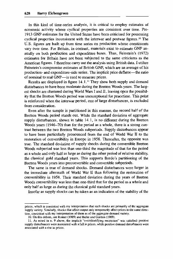
In this kind of time-series analysis, it is critical to employ estimates of economic activity whose cyclical properties are consistent over time. Pre- 1913 GNP estimates for the United States have been criticized for possessing cyclical properties inconsistent with the interwar and postwar figures.l0 The U.S. figures are built up from time series on production whose constituents vary over time. For Britain, in contrast, materials exist to estimate GNP an- nually on both production and expenditure bases. Thus, Feinstein’s (1972) estimates for Britain have not been subjected to the same criticisms as the American figures. I therefore carry out the analysis using British data. I utilize Feinstein’s compromise estimates of British GNP, which are an average of his production- and expenditure-side series. The implicit price deflator-the ratio of nominal to real GNP-is used to measure prices.

Results are displayed in figure 14.1 . I t They show both supply and demand disturbances to have been moderate during the Bretton Woods years. The larg- est shocks are clustered during World Wars I and 11, leaving open the possibil- ity that the Bretton Woods period was unexceptional for peacetime. This point is reinforced when the interwar period, one of large disturbances, is excluded from consideration.

Even after the sample is partitioned in this manner, the second half of the Bretton Woods period stands out. While the standard deviation of aggregate supply disturbances, shown in table 14.1, is no different during the Bretton Woods years (1946-70) than for the period as a whole, there is a strong contrast between the two Bretton Woods subperiods. Supply disturbances appear to have been particularly pronounced from the end of World War I1 to the restoration of convertibility in Europe in 1958. Thereafter, the opposite was true. The standard deviation of supply shocks during the convertible Bretton Woods subperiod was less than one-third the magnitude of that for the period as a whole and only half as large as during the other period of relative stability, the classical gold standard years. This supports Bordo’s partitioning of the Bretton Woods years into preconvertible and convertible subperiods.

The same is true of demand shocks. Demand disturbances were larger in the immediate aftermath of World War I1 than following the restoration of convertibility in 1958. Their standard deviation during the years of Bretton Woods convertibility was less than one-third that for the period as a whole and only half as large as during the classical gold standard years.

Insofar as supply shocks can be taken as an indication of the stability of the

prices, which is consistent with my interpretation that such shocks are primarily of the aggregate supply variety. Similarly, shocks that affect output only temporarily affect prices in the same direction, consistent with my interpretation of them as of the aggregate demand variety.

10. On this debate, see Romer (1989) and Balke and Gordon (1989). 1 1 . As noted in n. 9 above, the implicit “overidentifying restriction” was satisfied: positive

supply disturbances were associated with a fall in prices, while positive demand disturbances were associated with a rise in prices.

629 Epilogue

-0.05

-0.10

. I

a , I .

1 ' 1 i i -

- I

~. . . . . . . Demand ?

- supply

i -

Fig. 14.1 Aggregate supply and aggregate demand shocks, 1874-1975

Table 14.1 Standard Deviation of Supply and Demand Disturbances for Great Britain, Various Subperiods

~

Period Supply Demand

1874-191 3 ,015 .017 1946-70 .025 ,015 1946-58 ,033 ,020 1959-70 ,008 .008

Source: See text.

environment while demand shocks can be taken to indicate the stabilizing or destabilizing influence of demand management policy, this evidence suggests that both the underlying environment and policy contributed to the stability of output growth between 1959 and 1971. Global economic conditions may have been fortuitous for the operation of a pegged-rate system, but policy also played a part.

14.2.3 Contributions of Bretton Woods to Output Stability

A first channel through which the Bretton Woods system could have stabilized output was by influencing the formulation of monetary and fiscal policies. Table 14.2 reproduces evidence from Bordo (chap. 1 in this volume) on money growth rates and supplements it with the growth of real government


Table 14.2 Rates of Growth of Money Supply and Real Government Spending (% per annum)

~ ~

Money Growth

U.S. Canada Japan France Germany Italy U.K.

Gold standard (1881-1913) Mean Standard deviation Grand mean Convergence Interwar (1919-38) Mean Standard deviation Grand mean Convergence Bretton Woods (1946-70) Mean Standard deviation Grand mean Convergence Preconvertible Bretton Woods ( I 94658) Mean Standard deviation Grand mean Convergence Postconvertible Bretton Woods (1959-70) Mean Standard deviation Grand mean Convergence Floating (1974-89) Mean Standard deviation Grand mean Convergence

1.8 5.0 1 .o 1 .o

.6 8.6 2.0 1.7

6.3 5.8

10.1 4.2

6.4 8.3

11.4 6.0

7.0 1.5 9.8 2.5

8.6 2.4 9.5 2.7

Gold standard (1881-1 913) Mean Standard deviation Grand mean Convergence Interwar (1919-38) Mean Standard deviation Grand mean Convergence Bretton Woods (1946-70) Mean Standard deviation

0.4 4.6 -.O 1.4 5.5 5.0

1.1 .5 6.4 4.7 9.7 8.5

6.0 17.3 11.5 4.0 15.9 7.5

5.0 18.2 14.7 3.9 18.5 7.2

9.4 14.6 8.6 4.3 2.5 6.6

11.0 5.7 8.8 5.5 6.2 3.4

.6 .6 .3 2.6 3.2 3.1

1.3 3.6 .8 10.1 6.2 4.7

12.8 13.3 3.2 6.0 7.8 3.2

17.6 15.9 1.7 5.6 10.5 2.9

10.9 12.4 5.5 4.7 2.0 2.9

5.7 13.4 13.5 4.5 4.9 5.6

Real Government Spending Growth

3.2 5.7 10.3 1.5 5.6 4.5 2.5 9.3 13.4 31.2 5.4 9.3 2.4 .8 4.6 2.0

1.3 .6 10.3 4.8 6.5 6.8 -3.1 23.8 13.7 14.6 22.2 11.4 47.8 14.2

3.6 3.8

1.1 1.8 7.0 7.6 7.9 8.6 .2 17.6 13.9 11.2 18.0 13.6 10.6 9.5

631 Epilogue

Table 14.2 (continued)

Money Growth

U.S. Canada Japan France Germany Italy U.K

Grand mean Convergence Preconvertible Bretton Woods (1946-58) Mean Standard deviation Grand mean Convergence Postconvertible Bretton Woods ( I 959-70) Mean Standard deviation Grand mean Convergence Floating (197449) Mean Standard deviation Grand mean Convergence

4.7 3.4

-2.2 -1.6 2.3 13.3 1 1 . 1 8 . 7 - 3 . 9 23.4 18.2 16.1 25.9 10.2 12.2 10.2 3.1 5.9

4.7 5.7 10.1 3.4 5.8 8.6 4.8 5.1 4.2 3.1 5.3 15.0 8.6 4.9 6.1 1.8

4.0 5.3 8.7 3.3 2.0 6.5 4.8 3.0 4.6 4.1 3.0 3.3 5.9 8.8 4.8 1.6

Sources: For money, Bordo (chap. 1 in this volume). For government spending, Mitchell (1975, 1983) and the references cited therein. (The GNP deflator used to normalize nominal spending is also from Bordo . )

spending.12 For the G7 countries, money growth rates were more stable during the years of Bretton Woods convertibility than in any comparable period before or since. Their standard deviation was lower than during both the classical gold standard years and the period since 1973. When stability is measured by the coefficient of variation (the standard deviation divided by the mean), the years of Bretton Woods convertibility stand out even more dramatically.

Two conditions must be satisfied before we may conclude that the Bretton Woods system was responsible for the stability of money growth: first, that money growth was stable in the center country, the United States, which re- tained some monetary autonomy; and, second, that the exchange rate system forced other countries to emulate the U.S. example. Table 14.2 confirms that U.S. money growth was exceptionally stable during the years of Bretton Woods convertibility. But even if U.S. policy was stable, Bordo’s results suggest that Bretton Woods institutions forcing other countries to follow the U.S. example cannot account for monetary stability elsewhere. His measures of convergence do not indicate exceptionally close harmonization of monetary polices during the Bretton Woods convertible years. The average deviation of individual countries’ money growth rates from the subperiod grand mean was smaller during the gold standard years and even during the interwar period. The variability of that deviation has been smaller since 1974.

12. Nominal government expenditure is divided by the GDP deflator.


That other countries were not forced to closely emulate U.S. monetary policies and that their inflation rates consequently differed, two facts documented in Stockman (chap. 6 in this volume), again point to the prevalence of capital controls. Capital controls reconciled exchange rate stability with national monetary autonomy. The degree of monetary autonomy, as measured by the international inflation differential, should not be exaggerated, however. Infla- tion differentials can be observed even when monetary independence is limited. Even if trade and capital controls are absent and market integration is complete, one should still not expect to see identical inflation rates across countries. Opportunities are limited for international arbitrage in nontraded goods, and the relative price of nontradables tends to be low in low-income countries (the Balassa effect). Thus, the relative price of nontradables will rise most quickly where productivity growth is fastest. Even if arbitrage equalizes the prices of traded goods across countries, one should expect to see the consumer price index rise most quickly in those countries with rapid productivity growth.

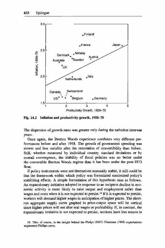
Even if the Balassa effect exists, it may not have had an economically important effect on inflation differentials across Organization for Economic Co- operation and Development (OECD) countries during the Bretton Woods years. Figure 14.2 arrays Maddison’s (1982) estimates of labor productivity growth between 1950 and 1970 against the rate of CPI inflation.I3 It confirms a point made by Obstfeld (chap. 4 in this volume): that the U.S.-Japan inflation differential is consistent with Balassa’s story. But it also makes clear that the power of the relation hinges on the inclusion of Japan. When this one observation is omitted from the sample of industrial countries, the productivity-inflation correlation vanishes. Additional factors besides productivity growth, plausibly including capital controls and divergent monetary policies, thus must be invoked in order to account for differences in inflation performance. l4

Turning from monetary to fiscal policy, the second panel of table 14.2 shows measures of the rate of growth of real government spending.I5 At 4.7 percent, the average annual rate of growth of real government spending under Bretton Woods was virtually the same as during both the classical gold standard years and the post-1973 float. But the variability of the growth of real public spending across countries, as measured in the rows labeled “convergence,” was higher during Bretton Woods than in either of the other periods.

13. Labor productivity is measured as output per man-hour, while inflation is measured as the ratio of Maddison’s CPI in 1970 to 1950. Note that Balassa formulated his effect in terms of the behavior of GDP deflators rather than consumer price indices, which include import prices. The distinction is irrelevant if the law of one price holds for traded goods.

14. One way of reinforcing the point is to observe that, if Germany as well as Japan is removed from the sample, evidence of the Balassa effect is strengthened. Germany pursued an exceptionally restrictive anti-inflationary monetary policy behind the shelter of capital controls, which explains why it is an outlier.

15. Sources of the GDP deflators are described in the appendix in Bordo (chap. 1 in this volume), while data on government expenditure are drawn from Mitchell (1975, 1983) and updated using the national sources he cites.

633 Epilogue

+Finland

+France Japan +/

+ Norway Denmark +

r- 0 2.51 l.

r

c - c - c 2.0 1 ++/ / Netherlands +'-

Canada Switzerland

Belgium +Germany 1 1 , ..,

1 2 3 4 5 Productivity Growth, 1950-70

Fig. 14.2 Inflation and productivity growth, 1950-70

The dispersion of growth rates was greater only during the turbulent interwar years.

Once again, the Bretton Woods experience combines very different per- formances before and after 1958. The growth of government spending was slower and less variable after the restoration of convertibility than before. Still, whether measured by individual country standard deviations or by overall convergence, the stability of fiscal policies was no better under the convertible Bretton Woods regime than it has been under the post-1973 float.

If policy instruments were not themselves unusually stable, it still could be that the framework within which policy was formulated maximized policy's stabilizing effects. A simple formulation of this hypothesis runs as follows. An expansionary initiative adopted in response to an incipient decline in economic activity is more likely to raise output and employment rather than wages and costs when it is not expected to persist.16 If it is expected to persist, workers will demand higher wages in anticipation of higher prices. The short- run aggregate supply curve graphed in price-output space will be vertical since higher prices will not alter real wages or profitability. If, in contrast, the expansionary initiative is not expected to persist, workers have less reason to

16. This, of course, is the insight behind the Phelps (1967jFriedman (1968) expectations- augmented Phillips curve.


worry about the inflation-induced erosion of their real incomes, and they will not be as insistent in demanding compensation in the form of higher nominal wages. The short-run aggregate supply curve graphed in price-output space will be positively sloped since higher prices reduce real production costs and enhance profitability. Demand stimulus will produce additional output and employment rather than higher wages and prices. Policy will retain some capacity to stabilize the macroeconomy.

How do these points relate to Bretton Woods? America’s stated policy of pegging the dollar to gold at $35.00 an ounce and foreign governments’ desire to peg their currencies to the dollar at prevailing parities may have been interpreted as commitments to a nominal anchor that reduced the perceived probability of persistent inflation, at least toward the start of the convertible Bretton Woods period, when the stability of declared parties was beyond doubt. Agents perceived that countries could not pursue consistently inflationary policies given their commitment to the maintenance of Bretton Woods. Hence, one-time policy initiatives affecting the price level were more likely to stabilize output and employment and less likely to be neutralized by offsetting changes in wages and costs.

Two points about this thesis are worth noting. First, it is quite revisionist relative to the older literature (Mundell 1963; Fleming 1962), which argued that monetary policy is less effective under fixed than floating rates. Accord- ing to my thesis, monetary policy can be more effective under fixed rates so long as it is formulated in a manner consistent with the maintenance of those rates. The eason is that monetary policy has different supply-side effects depending on the regime within which it is formulated. (Recall that the Mundell-Fleming model takes output and employment as demand determined.) In contrast, it is consistent with a subsequent literature (e.g., Dorn- busch and Krugman 1976) that argued that floating rates steepened the short- run Phillips curve trade-off.

Second, this view is quite consistent with growing complaints in the late 1960s on the part of monetary policymakers about the capital account offset to monetary policy. So long as the nominal anchor was credible, the capital account offset was small. Higher prices unaccompanied by higher wages, one consequence of which was higher output and employment, also stimulated money demand. Much of the additional money was willingly held; only a fraction leaked abroad through the balance of payments. Once the nominal anchor began to drag, output and employment did not increase; hence, the demand for money did not rise commensurately, and the monetary injection was offset through the capital account.

Evidence on this issue is provided by Alogoskoufis and Smith (1991), who estimate time-series models for inflation in the United Kingdom and the United States spanning the period 1857-1987. They find that an AR(1) process for inflation is an adequate univariate representation for both countries. The coefficients differ significantly across periods, however. For both coun-

635 Epilogue

tries, the coefficient on lagged inflation is larger after World War I than before. Moreover, there is evidence of a further rise in its magnitude coincident with the breakdown of Bretton Woods in the early 1970s.

Alogoskoufis and Smith then estimate an expectations-augmented Phillips curve in which the change in wage inflation depends on unemployment and on the lagged change in prices.” The coefficient on lagged inflation in this wage-change equation shows the same tendency to rise during World War I and again following the breakdown of Bretton Woods. This supports the notion, described above, that monetary policies affecting prices produced smaller increases in wages and larger increases in output and employment during the Bretton Woods period, when inflation was not expected to persist, than subsequently.

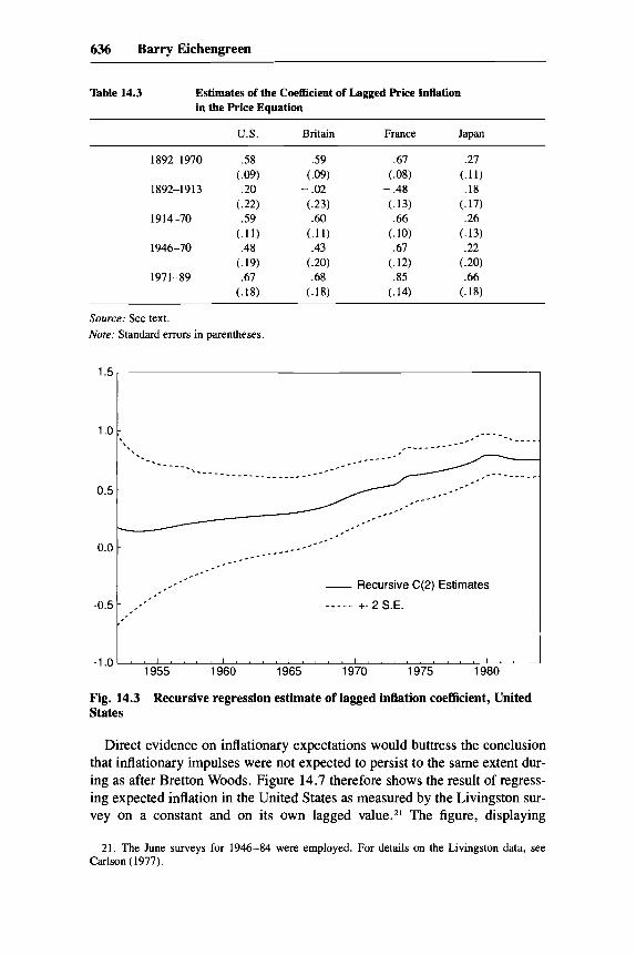
Table 14.3 replicates Alogoskoufis and Smith’s U.S. and U.K. inflation regressions, but for subperiods more precisely distinguishing the Bretton Woods years. It reports comparable regressions for two additional countries: France and Japan.’* For each of the countries considered, the coefficient on lagged inflation is larger after World War I than before. More important for present purposes, for each of the four countries the coefficient on lagged inflation is larger after the Bretton Woods period than during it.

Recursive regression estimates similar to those of Alogoskoufis and Smith for the period starting in 1948 show a tendency for the coefficient on inflation persistence to rise between 1970 and 1973, the time of Bretton Woods’s breakdown. These estimates are derived by first running the regression with a min- imum of degrees of freedom and then adding the observation for each subsequent year. For Britain and the United States, the tendency for the point estimate to rise when post-1971 data is added is evident whatever year in the second half of the 1940s the sample starts.Ig (Plots of the point estimates are displayed in figs. 14.3 and 14.4.) For France, a post-1971 rise in the coefficient estimate is apparent only if one excludes the immediate post-World War I1 years, a period characterized by unusual inflation persistence. For Japan, in contrast to table 14.3, the recursive regression estimates show little evidence of increasing inflation persistence (see figs. 14.5 and 14.6).20

17. Consumer or retail price indices are used. Wages and prices are lagged before differencing, while both current unemployment (differenced) and lagged unemployment (in levels) are included as regressors.

18. Price data for the United States and the United Kingdom are from the sources used by Alogoskoufis and Smith, while consumer price indices for other countries are from Maddison (1982). Efforts to estimate such an equation for Germany are hindered by a break in the price index in 1923-24. The results in table 14.3 differ from those of Alogoskoufis and Smith by the time periods chosen. Their definition of the Bretton Woods period extends from 1948 to 1967, not from 1946 to 1970 as here and in Bordo’s chapter. Similarly, they do not distinguish the preconvertible and convertible Bretton Woods subperiods. Their data set ends in 1987, mine in 1989.

19. The results are consistent with the earlier analyses of Klein (1975) and Barsky (1987). 20. Interestingly, France and Japan are the two countries for which Obstfeld (chap. 4 in this

volume) finds little evidence of price stickiness for the Bretton Woods period as a whole.


1.0

0.5

Table 14.3 Estimates of the Coefficient of Lagged Price Inflation in the Price Equation

- - _ _ _ ,---_ ,______-----

-

-----_____.___---- * - - - - - _ _ _ _ * - - _ _ _ - - - _ _ *.--

-

U.S. Britain France Japan

1892-1970 .58

1892-1 9 13 .20 (.22)

1914-70 .59 (. 11)

1946-70 .48

1971-89 .67

~ 0 9 )

~ 1 9 )

Source: See text. Nore: Standard errors in parentheses.

1.5,

1980 -1.01 ' ' 1 " ' ' I " " I ' " " 1 ' " I ' ' ' ' I "

1955 1960 1965 1970 1975

Fig. 14.3 Recursive regression estimate of lagged inflation coefficient, United States

Direct evidence on inflationary expectations would buttress the conclusion that inflationary impulses were not expected to persist to the same extent during as after Bretton Woods. Figure 14.7 therefore shows the result of regress- ing expected inflation in the United States as measured by the Livingston survey on a constant and on its own lagged value.21 The figure, displaying

21. The June surveys for 1946-84 were employed. For details on the Livingston data, see Carlson (1977).

637 Epilogue

-0.5

-1 .o

- , *.--

-'t:

, I , ,

- Recursive C(2) Estimates

_ _ _ _ _ +- 2 S.E.

1.0

0.5

0.0

- 1 . 5 1 " ~ ~ ~ ~ ~ ~ ~ ~ ~ ' ~ ~ ~ ~ ~ ~ ~ " ~ ~ ~ ~ ~ ' ~ 8 & A , I ) ' )

1955 1960 1965 1970 1975 1980 1985

Fig. 14.4 Recursive regression estimate of lagged inflation coefficient, Britain

a <

- ; '* I . a -. . . . . . . . . . . . . . . . . . . . . . _ _ _ _ - - - - -

,- ------______. - - - - _ _ _ _ - _ - - - - - I *.*

_ _ _ _ _ _ _ _ _ - - - - - - -

,- -

-0.5

-1.0

_ _ _ - - - - _ _ _ _ - - - - - _ - - - _ _ - - _ _ - - .-- -

- Recursive C(2) Estimates I I +

$ 8 , I I t * I

_ - - _ - +- 2 S.E. -:, ;

, I

-1.51 ' ' ' ' ' ' ' I ' ' ' ' I . ' ' ' I ' ' ' ' ' ' ' ' ' I ' ' ' 1960 1965 1970 1975 1980 1985

Fig. 14.5 Recursive regression estimate of lagged inflation coefficient, France


1.25

1 .oo

0.75

0.50

0.25

0.00

-0.25

_ _ _ _ _ +- 2 S.E.

I , , , , I , , , . I , , . , I . , . , 1 , . , , / , , . , I I I .

1955 1960 1965 1970 1975 1980 1985

Fig. 14.6 Recursive regression estimate of lagged inflation coefficient, Japan

0.75

0.50

0.25

0:oo

-0.25

-0.50

-0.75

,---__

- Recursive C(2) Estimates

_ _ _ _ _ +- 2 S.E.

- - - - _ _ _ _ _ _ - - * - _ - - _ _ - - - _ - - _ _ .-__

_ - - _ _ _ - - _ _ - - - . . . . . . . . . . . . . . . . . . . . . . . .

_ - - -

I I . . . I . I / I I , , I I I I I . I I . I . I I . . . 1955 1960 1965 1970 1975 1980

Fig. 14.7 Recursive regression estimates of lagged expected inflation on expected inflation

639 Epilogue

recursive regression estimates of the coefficient on lagged expectations, shows the increasing persistence of inflationary expectations in the 1970s. A Chow test for a sample break in 1971 rejects the null of structural stability at the 95 percent confidence level.

I also regressed expected inflation over the coming twelve months on actual inflation over the preceding twelve months. The top left-hand panel of figure 14.8 displays the recursive regression estimates of the lagged inflation coefficient. Prior to 1970, there is essentially no tendency for lagged inflation to engender inflationary expectations. Subsequently, lagged inflation has a persistent and growing effect on inflationary expectations. The same is true for inflation lagged twenty-four, thirty-six, and forty-eight months, as shown in the other panels of figure 14.8. In each case, a Chow test rejects the null of structural stability across the 1971 break point.

To reiterate the implications of these findings, there is evidence of increasing inflation persistence following the breakdown of Bretton Woods. From survey data it is clear that this persistence was perceived by agents, and from Phillips curve estimates it appears that this perception was incorporated into wage-setting behavior. Thus, it was easier before 1971 than after for policymakers to use monetary and fiscal policies to manipulate output and employment because policies with inflationary consequences were not expected to persist and hence their short-run stimulative effects were not neutralized by higher wages and costs.22 Stabilization policy was more effective because it was formulated within a framework, namely the Bretton Woods system, that provided a credible price-level anchor. Once policy began to be formulated in a manner incompatible with that framework, the anchor began to drag. The Bretton Woods system was not the only casualty: other victims were the effectiveness of stabilization policy and the stability of output, as problems of time consistency and credibility reared their heads.

14.2.4 The Role of the IMF

As we saw in the previous section, Bretton Woods’s par values and governments’ commitment to them could have enhanced the credibility of policymakers’ dedication to price stability and heightened the effectiveness of their actions. This raises the question of why par values were respected, rather than being manipulated as they had been in the 1930s. A possible answer is that the establishment of the IMF altered the costs and benefits of alternative courses of action.

One variant of this hypothesis focuses on the time-consistency problem developed in a monetary context by Kydland and Prescott (1977). Policymakers with an incentive to repeatedly fool the public by running higher-than- anticipated inflation could have been reined in by an International Monetary

22. This, of course, is the point of Lucas’s classic American Economic Review article (Lucas 1973).

Recursive Regression Estimates of Effect of Lagged Inflation on Inflationary Expectations

Recursive Regression Estimates of Effect of Inflation Lagged Twice on Inflationary Expectations

0.75 1 0.75 II I 0.50

0.25

0.00

- - - - _ -

- - - _ _ - - _ _ - '-., -

-0.751.' . ' . . I . . . . a . . . . I . . . . I . . . . a , . . I 1955 1960 1965 1970 1975 1980

-0.25

-0.50-

_ - - 0.50 1 ,-

_---' _ _ _ _ _ _ _ _ _ - - - - - - - * _ - - -

- _ - - - _ ,_-- _-. - - - - _ _ _ _ _ _ - * 0.00

-0.25 .--

0.5

0.4

___I _ _ _ _ - - - - - - - _ _ _ _ - - -0.50 I, ,_.-----

,-. I .-

:,\

- '., -

Recursive Rearession Estimates of Effect of Inflation Recursive Rearession Estimates of Effect of Inflation

-0.1 -0.2

Lagged Three Times on Inflationary Expectations 0.50 I I

I - - ,--__: - - _ _ - - - _ _ - - - - - - - - .;- - _ - - - -

-___---__I - - _ _ _ - _ _ _ - - - - - - - -

-0.50 - a c t - - 1955 1960 1965 1970 1975 1980

-0.75 I . . a . . . . a . , . . I . . , . I . , . I , . . , . , . I

Recursive C(2) Estimates

Fig. 14.8 Recursive regression estimates of effect of lagged inflation on inflationary expectations

641 Epilogue

Fund able to prevent the pursuit of persistently inflationary policies. The Fund thus provided a “commitment technology” that solved the time-consistency problem. Another variant of the hypothesis focuses not on this game between policymakers and the public but on a parallel game between domestic and foreign governments. The problem here is that governments might pursue policies that work to their national advantage but throw off negative externalities, destabilizing the international monetary system. If, for example, the advan- tages of maintaining a pegged exchange rate are positively related to the number of other countries that do the same, intervention by the Fund to discourage unilateral devaluation could have enhanced the stability of the system.

One can imagine various ways in which the IMF could have enhanced the stability of the system or provided a commitment technology. It could have been the enforcer of rules that proscribed beggar-thy-neighbor devaluations and macroeconomic policies with unsustainable balance-of-payments consequences. As shown by Giovannini (chap. 2 in this volume) and Ikenberry (chap, 3 in this volume), such rules were proposed by the United States in early stages of the Bretton Woods negotiations. But binding restrictions on international economic policies were removed at the behest of the United Kingdom. An escape clause-that countries were justified in devaluing uni- laterally in the event of “fundamental disequilibrium”-was added to the agreement. It is impossible therefore to interpret the Fund’s role as enforcer of hard-and-fast rules.

While not the enforcer of formal rules, the Fund could still have influenced governments’ choice of policies by offering pecuniary incentives. Drawings and loans from the Fund could have reduced the effect on living standards of domestic adjustments needed to restore balance-of-payments equilibrium, or at least allowed governments to stretch out that burden over time. Pecuniary incentives could have increased the likelihood that countries would undertake the adjustments needed to restore balance-of-payments equilibrium and avoid policies tending to destabilize the system and undermine its credibility.

Dominguez (chap. 7 in this volume) pours cold water on enthusiasts of this view. She shows that only five countries were officially denied access to IMF resources over its first twenty years of operation.23 Moreover, one can imagine the availability of IMF credit had the same effect on government behavior as deposit insurance has on a bank-that is, it could have encouraged risk taking by offering a bailout. Evidence presented by Edwards and Santaella (chap. 8 in this volume)-that countries running especially expansionary policies and suffering large deteriorations in their balance-of-payments positions tended to turn to the IMF for assistance when devaluing-is consistent with this moral hazard view.

That only a handful of countries were denied access to IMF resources in its first two decades of operation may be too narrow a basis for evaluating the

23. Much the same pint is made by Argy (1981).


sanctions and rewards at the Fund’s disposal. Drawings on the Fund become increasingly important, in quantity and number, after 1966. In any case, the organization’s leverage may have been largely independent of its current financial exposure. Reneging on an agreement with the Fund could have had costs, even in the absence of current IMF drawings, insofar as the Fund and the country were engaged in a repeated game on whose outcome the future availability of financial resources hinged. The negotiation of a Fund agreement could thereby provide the needed commitment technology. Edwards’s evidence that weak governments had a disproportionate tendency to solicit IMF support for devaluation-cum-adjustment programs can be interpreted to suggest that the Fund’s “seal of approval” was important for enhancing the credibility of governments lacking a reputation for implementing painful adjustment programs.

Finally, once international bank lending started up in the 1960s, commercial banks typically required that countries experiencing balance-of-payments difficulties reach an agreement with the Fund for a standby loan as a precondition for rescheduling and renewed lending. For countries in external crisis, the Fund had veto power not just over the extension of its own resources but over commercial bank lending as well. Thus, the Fund could have exercised leverage through its signaling role. It is revealing that, in the nineteenth century, simply going onto the gold standard was the only signal lenders required that a country had put its international financial house in order; as soon as gold convertibility was restored, lending resumed (Fishlow 1989). After World War 11, lenders required a standby agreement as well as a stable exchange rate, another indication that stated commitments to stabilize rates were imperfectly credible.

Even if the Fund did not directly enforce rules, provide rewards, or impose penalties, it could have facilitated the efforts of others to do so. Drawing on the theory of strategic games with incomplete information, Dominguez (chap. 7 in this volume) shows how the threat of retaliation can sustain cooperation. The prospect that other nations will retaliate against countries that adopt policies jeopardizing the stability of the system may suffice to prevent those policies from being pursued. The more costly it is to obtain information on a government’s policy, however, the more likely it is that it will escape retaliation when acting noncooperatively. The acquisition and dissemination of information, Dominguez argues, was the most important role of the IMF. Non- cooperative behavior was thereby discouraged and systemic stability enhanced.

There exists no ready measure of the informational value added of Fund missions and of publications like International Financial Statistics. If we are concerned with the leading industrial countries, those with the greatest capacity to destabilize the international monetary system, then it is hard to imagine that, in the absence of the IMF, the treasuries and central banks of the G7

643 Epilogue

countries could not have gathered information on one another’s actions at relatively low cost. In the Fund’s absence, moreover, the OECD or the Bank for International Settlements (BIS) surely would have developed an analogous informational role.

Even if its surveillance of the G7 countries was of little moment, the Fund may have made more of a difference in the case of smaller, developing countries. One of the prominent differences between the post-1958 Bretton Woods system and the interwar and classical gold standards was the sheer number of players in the international monetary arena. The Fund surely facilitated efforts to monitor the actions of the smaller players and thereby helped minimize the free-rider problems that might otherwise have resulted from the large-numbers problem.

14.2.5 The Role of Capital Controls

Students of the post-1979 European Monetary System (EMS) typically are skeptical that Bretton Woods’s adjustable peg could have functioned in the absence of capital controls (see Giovannini 1989). In its early phases, the EMS successfully reconciled divergent national policies with exchange rate stability by restricting international capital movements (see Giavazzi and Giovannini 1989). Hence, market forces did not require EMS members seek- ing to peg their exchange rates to continuously pursue monetary policies consistent with interest-rate equalization. Interest rates and monetary policies could differ because capital controls increased the cost of financial arbitrage. When international inflation differentials had persisted for a sufficient length of time for the competitiveness of the high-inflation country to be eroded, a discrete realignment of exchange rates was required, after which another period of exchange rate stability could ensue. In recent years, Europe’s capital controls have essentially been removed. Economic policies have converged, and realignments have become infrequent.

Viewing Bretton Woods through EMS-tinted glasses suggests that it too relied on capital controls for reconciling policy autonomy with exchange rate stability. The United Kingdom, which experienced a series of balance-of- payments crises, maintained an array of controls on direct and portfolio investment abroad. The U.S. Interest Equalization Tax imposed in 1963 was clearly intended to reconcile domestic stimulus with an increasingly worri- some external position. But surplus as well as deficit countries utilized capital controls during the Bretton Woods years, as Giovannini (1989) points out. For example, in 1961 and again in 1970, the Bundesbank imposed discriminatory measures meant to discourage foreign residents’ purchases of German assets in order to limit the deutche mark’s appreciation.

This is an important difference between Bretton Woods and the pegged-rate systems of the nineteenth century and the 1920s. Contrary to Stockman’s (1987) suggestion that capital controls are always more prevalent in periods of


fixed nominal rates, they were all but absent in the late nineteenth century and the second half of the 1 9 2 0 ~ . ~ ~ The explanation is the very different weight attached to domestic policy autonomy. Capital controls were not needed in the nineteenth century or the 1920s to reconcile exchange rate stability with policy independence since discretionary policy was largely beyond the ken of governments. In the 1960s, when the influence of Keynesian theory was at its height, the case for capital controls to facilitate intervention was particularly compelling. As discretionary policy fell from favor, so did capital controls. Hence, Europe has moved away from capital controls designed to reconcile exchange rate stability with monetary autonomy, leaving no scope for monetary independence.

The EMS analogy also raises the question of whether the growing inflexi- bility of pegged rates in the late Bretton Woods period reflected the declining effectiveness of capital controls. As financial market participants discovered new ways of circumventing controls, were governments less able to change their parities because even contemplating the option risked provoking a speculative attack? Evidence presented by Marston (chap. 11 in this volume), summarized in his figure 11.3, lends little support to this view. The Eurodol- lar-domestic CD rate differential, one measure of the effectiveness of U.S. controls, widened rather than narrowing in the final years of Bretton Woods. Yet it is possible that other factors were working to widen the differential even while the effectiveness of capital controls was being undermined. (Regulation Q restrictions in the United States, e.g., grew increasingly binding as U.S. inflation accelerated. Case studies for other countries [e.g., Hewson and Sa- kakibara 19771 support the notion that the effectiveness of controls was being eroded.) Ultimately, however, this factor must be weighed against other potential explanations for the collapse of Bretton Woods.

14.2.6 The Collapse of Bretton Woods

Why the pegged-rate system collapsed is among the most contentious and confusing debates in the literature on the Bretton Woods system. A first distinction helpful for sifting through the alternatives discriminates between explanations focusing on policy imbalances and those emphasizing instead flaws in the structure of the system. A second distinction further subdivides explanations focusing on policy imbalances into those emphasizing increasingly inflationary monetary policy in the United States and those attaching priority to fiscal policy.

The explanations stressing policy imbalances find support in the data, although the strength of the backing depends on the measure of policy that is

24. Here I differ from the conclusion of Giovannini (1989). While there was some use of the “gold devices” to temporarily limit the incentive for arbitrage in the gold and foreign exchange markets after 1880, I find it hard to classify these measures as “capital controls.” In any case, their effects were small compared to the wedge between domestic and foreign interest rates created by the capital controls of the 1960s. As I show elsewhere (Eichengreen 1991), capital controls were all but absent under the interwar gold standard.

645 Epilogue

preferred. Figure 1.31 in Bordo’s chapter in this volume juxtaposes the growth of the monetary base (domestic credit plus international reserves) against the growth of domestic credit alone, revealing that the U.S. authorities were expanding domestic credit at a relatively rapid rate throughout the period. They allowed the monetary base to continue to expand despite the loss of reserves. Moreover, the gap between the growth rates of the base and of domestic credit widened noticeably in 1968-69 as the collapse of Bretton Woods loomed, a point also emphasized by Genberg and Swoboda (chap. 5 in this volume). This evidence favors the explanation for Bretton Woods’s collapse emphasizing excessively expansionary U.S. monetary policy. It is no- table, however, that the gap between the growth rates of domestic credit and the monetary base closed in the final years of Bretton Woods (1970-71), as if U.S. monetary policy finally began to conform to the dictates of the international system.

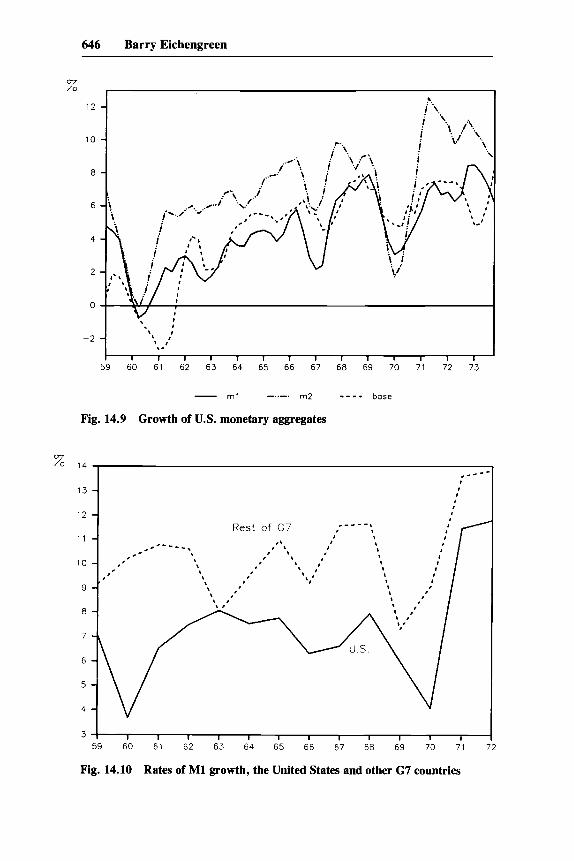
Figure 14.9 compares the growth of the monetary base with the growth of broader aggregates. Although the rates of growth of the broader aggregates, like the base, rose in the first part of the 1960s, supporting the notion that excessive monetary growth fueled U. S. balance-of-payments deficits and thereby tended to destabilize the dollar, they show less tendency to rise in the three or four years immediately preceding the collapse of Bretton Woods. In particular, MI growth displays little trend over the four years preceding the suspension of gold convertibility in 1971. Most of the action is concentrated in M2 growth, which fell markedly in the wake of the 1967 credit crunch but then rose to unprecedented levels as the collapse of Bretton Woods loomed. If money growth was responsible for Bretton Woods’s collapse, then it would appear that the problem was not merely the excessive expansion of domestic credit but also the Fed’s failure to react to the unprecedented divergence between the growth rates of M2 and the base in the years leading up to the crisis.

Figure 14.10 compares M1 growth in the United States and other G7 countries.25 It is less obviously supportive of the monetary hypothesis. There is no apparent shift in the relation between U.S. and foreign money growth rates that could have contributed to the breakdown of Bretton Woods. M1 growth is consistently slower in the United States than abroad, a fact superficially at odds with indictments of U.S. monetary policy as excessively expansionary. The explanation lies in the fact that the United States was growing more slowly than Europe and Japan throughout the period, limiting the growth of money demand. Observers warned that the international competitive position of the U.S. economy was deteriorating, worsening the country’s trade and payments position (for examples, see Solomon 1982). The implication was that U.S. money growth had to slow still further relative to foreign money growth in order to bring about a decline in American wages and costs suffi-

25. The figures for the rest of the G7 are unweighted averages of annual observations for the six countries. Data are taken from the sources listed in the appendix to Bordo (chap. 1 in this volume).


12 -

10 -

8 -

. I

. I t ,

\ I -2 - ,.

I I I I I I I I I I I I 1 I

59 60 61 62 63 64 65 66 67 68 69 70 71 72 73

m2 - - - - base - ml -..-.

Fig. 14.9 Growth of U.S. monetary aggregates

%

I I I 1 I I I I I I 1 I

59 60 61 62 63 64 65 66 67 68 69 70 71

Fig. 14.10 Rates of M1 growth, the United States and other 6 7 countries

647 Epilogue

cient to reconcile the nation’s competitive position with the maintenance of the existing set of dollar exchange rates.

A related school of thought blames growing U.S. budget deficits for fueling excessive demands for imports, thereby leading to the deterioration in Amer- ica’s external accounts. Figure 14.1 1 confirms the existence of a secular decline in the U.S. budgetary position in the 1960s. This is particularly evident in the shift from surplus to deficit in the high-employment budget balance, interrupted only by the exceptional surpluses of 1969.

While far from overwhelming, the evidence is at least consistent with some role for U.S. monetary and fiscal policies in Bretton Woods’s collapse. How much weight should be attached to these demand disturbances hinges in part on their magnitude. If we use the time-series methodology of section 14.2.2 above to quantify disturbances, it turns out that they were small compared to the demand disturbances typical of the subsequent period. Figure 14.12 shows the estimated supply and demand disturbances recovered from a two-variable VAR like that estimated above, but this time using data for the United States starting in 1960.26 Although there are positive demand disturbances in the mid-1960s and again in 1972-73, there is little evidence that demand rose relative to normal in 1969-71 or that the demand disturbances of the sur- rounding periods were large relative to those of the post-1973 years.

But, as Garber (chap. 9 in this volume) shows, a central implication of the recent literature on balance-of-payments crises is that a small disturbance can provoke a large balance-of-payments crisis. Even if the current increase in money supply and the current loss of reserves are small relative to the reserves that remain, they may still be just large enough to reduce reserves to a critical threshold at which a speculative attack occurs. And other policies, like budget deficits that increase the perceived probability that the monetary expansion will continue, advance the date of the attack.

As Garber points out, the timing of the speculative attack depends on the assets and liabilities of the public and private sectors and on the exchange rate that is expected to prevail subsequently. The larger the expected depreciation of the dollar following the breakdown of Bretton Woods, the larger the capital losses to be suffered by those holding dollars, and the earlier the date at which investors would bail out. Hence, as the competitive position of the U.S. economy deteriorated and forecasts of the magnitude of the dollar depreciation required to restore external balance were revised upward, the date of the speculative attack was advanced. Similarly, the larger the liquid dollar claims on the U.S. monetary authorities, the greater the incentive for each claimant to queue up at the gold window before others withdrew the remaining gold reserves. This is why contemporaries viewed the growth of U.S. external liabilities with alarm.

26. Data are drawn from the OECD national income accounts. These results and the figure are reproduced from Bayoumi and Eichengreen (1991).


2 5

2.0

1 5

1 0

0 5

0 0

-0 5

- 1 0

- 1.5

-2.0

Fig. 14.11 Measures of U.S. fiscal stance

3

- - - Supply Disturbances L . . .

- - Demand Disturbances

, ' I I ' , I ' I I ' I

-3 1963 65 67 69 71 73 75 77 79 81 83 85 87 89

Fig. 14.12 Aggregate supply and demand disturbances for the United States

3

649 Epilogue

It enhanced the influence of Robert Triffin’s warning that the Bretton Woods system was vulnerable to such an attack that his Gold and the Dollar Crisis, in which the alarm was sounded, was published in 1960, the very year in which U.S. external liabilities first exceeded U.S. monetary gold reserves. Discussion of the problem was renewed in 1963, when U.S. external liabilities to monetary authorities surpassed U.S. monetary gold. As Garber (chap. 9 in this volume) observes, however, it is not obvious that these external liabilities were the relevant measures of the dollar’s v~lnerability.~~ In principle, the government’s domestic liabilities could also be mobilized for a speculative attack. In 1964, when U.S. external liabilities came to $29 billion, U.S. M1 was an order of magnitude larger: $409 billion. If only a fraction of that $409 billion was sold for foreign currencies, the Fed and the Treasury would be confronted with much larger problems than whether foreigners remained willing to hold their $29 billion. Contemporary analysts focusing on the U.S. government’s external liabilities rather than its internal ones were presumably reassured by the existence of barriers to the conversion of domestically held dollars into foreign exchange. Once more, this testifies to their faith in the effectiveness of capital controls.

More restrictive U.S. policies would have limited the growth of both domestic and external claims on the U.S. government. Had the Fed reduced the rate of growth of American monetary liabilities so that they were slower to overwhelm U.S. gold reserves, the effort to peg the dollar price of gold at $35.00 might not have had to be suspended in 1968. The right to purchase gold at that price would not have had to be limited to foreign governments, and it would not have been necessary to apply moral suasion to the latter to desist. In other words, it might not have been necessary to transform the Bret- ton Woods gold-dollar system into a dollar standard.

Had American policymakers only played by the rules of the game, as the French were fond of putting it, Bretton Woods could have soldiered on. This understates the extent of the problem, however, since more restrictive U.S. policies would have led to an improvement in the U.S. balance of payments, depriving the rest of the world of international reserves. Assuming, as does Garber, that reductions in the price level were not viable, continued economic expansion impelled countries to acquire additional reserves. Given the inelas- ticity of global gold supplies and the limited rate at which special drawing rights (SDRs) were created, acquiring additional reserves meant acquiring additional dollars. Foreign governments, starved of dollars, in an effort to obtain them would have responded to monetary restriction in the United States with monetary restriction at home. The rise in prices and money supplies world- wide would have slowed relative to the rate of increase of global stocks of

27. Nor is it obvious that U.S. monetary gold was the relevant measure of assets to set against these liabilities, for U.S. monetary authorities could always purchase additional gold if they were willing to bear the costs associated with buying at a market price that exceeded $35.00 an ounce.


monetary gold. While the gold problem would have been deferred, at least temporarily, offsetting shifts in domestic and foreign monetary policies would not have strengthened the dollar exchange rate. There is no reason to think that the U.S. balance of payments would have improved significantly or that the run on the dollar would have been delayed beyond 1971.

Ultimately, then, the collapse of Bretton Woods was attributable as much to the structure of the system as to the specific policies pursued. Structural flaws dictated collapse sooner or later; policies at home and abroad determined only the timing of the event.

14.2.7 Implications for International Monetary Reform

In October 1991, when the NBER conference on Bretton Woods was held, the countries of the European Community were preparing to negotiate a monetary agreement leading to the establishment of permanently fixed exchange rates and, ultimately, a single currency for the participating countries. As is evident from the panel discussion that precedes this chapter, there existed at the conference considerable-although by no means universal-sentiment for stabilizing exchange rates over a wider area. What are the implications of the Bretton Woods experience for the desirability and structure of such international monetary reforms?

The most important implication is that simply stabilizing exchange rates is not sufficient to automatically deliver the benefits trumpeted by the propo- nents of such an initiative. The exchange rates of the major industrial countries were pegged to one another from the end of World War I1 until 1958 and adjusted only very occasionally, yet the output, interest rate, and real exchange rate stability that are supposed to be associated with stable nominal exchange rates did not follow. Even subsequently, nominal exchange rates were pegged for extended periods without promoting the international financial integration that is often thought to follow. There were wide differentials in the behavior of these variables across participating countries as well.

These observations speak to what is known in Europe today as the “convergence debate.” The question is whether, or, more precisely, to what extent, economic policies like budget deficits and economic outcomes like inflation must converge before countries enter into an agreement to fix exchange rates (for further discussion of this point, see Collins and Giavazzi, chap. 12 in this volume). The years of Bretton Woods inconvertibility (1946-58) confirm the feasibility of running a fixed rate system in the absence of convergence; at the same time they support those who argue that the maintenance of stable nominal rates in the absence of convergence can require capital controls and other expedients incompatible with reaping the full benefits of exchange rate stability. At odds with this position is the observation that the years of Bretton Woods convertibility (1959-71) indicate that it might still be possible to reap many of those benefits (interest rate stability, real exchange rate stability, out-

651 Epilogue

put stability) in the presence of capital controls and incomplete policy convergence.

One reconciliation of these points may lie in the fact that what is critical for the smooth operation of a system of stable exchange rates is not continual policy convergence per se but a commitment to exchange rate stability with sufficient credibility to reassure agents that policies will be consistent with stable exchange rates over the long term. Monetary and fiscal policies could and did diverge in the short run. But market participants were confident that industrial countries pegging to the dollar would eventually adjust their policies so as to reconcile them with the maintenance of a pegged dollar rate. So long as this remained the case, international capital movements stabilized nominal rates, rather than destabilizing them, until those policy adjustments took place. The relative stability of other variables followed.

Comparisons of Bretton Woods with the current situation also suggest that credibility-enhancing mechanisms and the rapid adjustments needed to render policies consistent with pegged exchange rates are even more important in Europe today and will be still more important to any future international monetary reform than they were to Bretton Woods. The devices that gave policymakers in the post-World War I1 period room to maneuver are no longer present. This refers not only to exchange controls but also to adjustments of the rate at which tariff barriers are reduced so as to strengthen the current account position of the initiating country or its trading partners. That there is no reason to anticipate another period of exceptional stability in the underlying economic environment comparable to the convertible Bretton Woods years rein- forces the point.

This emphasis on credibility is consistent with the argument for a European central bank and a single European currency in preference to Europe’s current system of pegged exchange rates between distinct currencies. It is argued that such institutional reforms are precisely what are needed to enhance the credibility of stated commitments to exchange rate stability. But even if it is viable in Europe, this same model is unlikely to be viable over a wider area. Euro- pean monetary unification is part of a larger bargain with political, social, and security dimensions. Countries that make concessions on the monetary front (Germany?) are presumably compensated when their partners make concessions on political or social questions. Even if it is completed on schedule, European monetary unification will be the culmination of nearly half a century of building the European Community. Although the events of the early 1990s caution us to remember how quickly and discontinuously the international environment can change, a comparably wide-ranging and time-consuming process will presumably be needed to extend such a monetary agreement to North America and Japan.

Bretton Woods itself drives home the point that ambitious designs for international monetary reform are viable only as part of a wider political and eco-


nomic bargain. As several of the papers in this volume remind us, the system of pegged but adjustable rates negotiated at the Mt. Washington Hotel was part of an agreement that involved the creation of an international bank, an international trade organization, and, implicitly, a set of international security arrangements. Yet, even at Bretton Woods, certain issues, like who would bear the cost of creating a synthetic reserve asset and how that asset would be distributed, were too explosive to be successfully negotiated. Consequently, in the 1960s, disputes over to whom SDRs should be distributed led them to be created first in insufficient numbers and then excessively. The conflict between adequate liquidity and U. S . balance-of-payments stability was therefore allowed to bring the system down.

If this premise is correct-that enduring international monetary reform is possible only as part of a larger political bargain and that even the extraordi- nary political consensus that united the United States and its allies in the final days of World War I1 was inadequate to permit the negotiation of a truly du- rable set of international monetary arrangements-then one is left deeply skeptical about the viability of a common currency or truly stable exchange rates for the entire world. Those like Richard Cooper (1989) who urge policymakers to consider a common currency for all the industrial democracies are then engaging in long-range planning of the most ambitious sort.

Appendix

In this appendix, I describe the VAR decomposition used in the text to identify aggregate supply and aggregate demand disturbances. The approach draws on Bayoumi (1991).

The methodological point of departure is the familiar aggregate demand- aggregate supply diagram shown in the top panel of figure 14A. 1. The aggregate demand curve (labeled AD) is downward sloping, reflecting the fact that, by raising money balances, lower prices boost demand. The short-run aggregate supply curve (SRAS) is upward sloping, reflecting the assumption that prices are sticky and hence that higher prices imply lower real wages. The long-run supply curve (LRAS) is vertical since real wages adjust to changes in prices in the long run.

The effect of a shock to aggregate demand is shown in figure 14A. lb. The aggregate demand curve shifts from AD to AD', moving the equilibrium from E to the new intersection with the short-run curve, D'. This raises both output and prices. As the aggregate supply curve becomes more vertical, the economy moves gradually from D' to D". Output returns to its initial level, while the price level rises permanently. Hence, the response to a positive demand

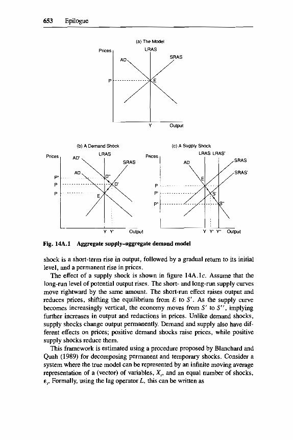
653 Epilogue

p p

p"

Prices

P

P

P

........................

............... - - - - S'

................... 8 s... s"

Prices

P

(a) The Model

LRAS

I

Y output

(b) A Demand Shock (c) A Supply Shock

A D

Y y' output

1 ,WAS'

I 1 ' I

Y y' y" Output

Fig. 14A. 1

shock is a short-term rise in output, followed by a gradual return to its initial level, and a permanent rise in prices.

The effect of a supply shock is shown in figure 1 4 A . l ~ . Assume that the long-run level of potential output rises. The short- and long-run supply curves move rightward by the same amount. The short-run effect raises output and reduces prices, shifting the equilibrium from E to S' . As the supply curve becomes increasingly vertical, the economy moves from S' to S", implying further increases in output and reductions in prices. Unlike demand shocks, supply shocks change output permanently. Demand and supply also have different effects on prices; positive demand shocks raise prices, while positive supply shocks reduce them.

This framework is estimated using a procedure proposed by Blanchard and Quah (1989) for decomposing permanent and temporary shocks. Consider a system where the true model can be represented by an infinite moving average representation of a (vector) of variables, X,, and an equal number of shocks, E,. Formally, using the lag operator L, this can be written as

Aggregate supply-aggregate demand model


(Al)

where the matrices A, represent the impulse response functions of the shocks to the elements of X .

Specifically, let X , be made up of the change in output and the change in prices, and let E, be demand and supply shocks. Then the model becomes

X , =AO&, + A I ~ , - I + A 2 ~ r - 2 + A,&,- , . . . r = O

where y , andp, denote the logarithm of output and prices, E ~ , and E,, are supply and demand shocks, and aI l i represents element ull in matrix Ai.

The framework implies that, while supply shocks have permanent effects on the level of output, demand shocks only have temporary effects. (Both have permanent effects on the level of prices.) Since output is written in first- difference form, the cumulative effect of demand shocks on the change in output (AyJ must be zero. This implies the restriction

m

, = O

The model defined by equations (A2) and (A3) can be estimated using vector autoregression. Each element of X , can be regressed on lagged values of all the elements of X . Using B to represent these estimated coefficients, the estimating equation becomes

X , = b , X , _ , + B,X,_, + . . . +B,X,-, + e,

= [ I - B(L)] - le,

= [ I + B ( L ) + B(L)2 + . . . ]e ,

= e, + D,e ,_ I + D2erP2 + D3er-, + . . . , where e, represents the residuals from the equations in the vector autoregression. In the case considered, e, is composed of the residuals of a regression of lagged values of Ay, and Ap, on current values of each in turn; these residuals are labeled ey, and ep,, respectively.

To convert (A4) into the model defined by (A2) and (A3), the residuals from the VAR, e,, must be transformed into demand and supply shocks, E,.

Writing e, = CE,, in the two-by-two case considered four restrictions are required to define the four elements of the matrix C. Two are normalizations, the convention being that the variance of the shocks E ~ , and E, is equal to unity. A third restriction comes from assuming that demand and supply shocks are orthogonal. These three restrictions define the matrix C to be any matrix such that CC’ = C, where C is the variance-covariance matrix of e,.

(A4)

655 Epilogue

The final restriction, which allows the matrix C to be uniquely defined, is that demand shocks have only temporary effects on output.28 As noted above, this implies equation (A3).29 In terms of the VAR, it implies

Note that this restriction says nothing about the effect on prices. The aggregate demand-aggregate supply model implies that demand shocks should raise prices in both the short and the long run while supply shocks should lower prices. Since these responses are not imposed, they can be thought of as overidentifying restrictions. 30

References

Alogoskoufis, George, and Ron Smith. 1991. The Phillips Curve, the Persistence of Inflation, and the Lucas Critique: Evidence from Exchange Rate Regimes. American Economic Review 8 1 ; 1254-75.

Argy, Victor. 1981. The Postwar International Monetary Crisis. London: Allen & Unwin.

Balke, Nathan, and Robert J. Gordon. 1989. The Estimation of Prewar Gross National Product: Methodology and New Evidence. Journal of Political Economy 97:38-92.

Barsky, Robert. 1987. The Fisher Hypothesis and the Forecastability and Persistence of Inflation. Journal of Monetary Economics 19:3-24.

Bayoumi, Tamim. 1990. Saving-Investment Correlations: Immobile Capital, Govern- ment Policy or Endogenous Behavior? IMF Staff Papers 37:360-87.

. 1991. The Effects of the ERM on Participating Economies. International Monetary Fund. Typescript.

Bayoumi, Tamim, and Barry Eichengreen. 1991. Shocking Aspects of European Mon- etary Unification. International Monetary Fund and University of California, Berke- ley. Typescript.

Blanchard, Olivier, and Danny Quah. 1989. The Dynamic Effects of Aggregate De- mand and Supply Disturbances. American Economic Review 79:655-73.

Blanchard, Olivier, and Lawrence Summers. 1986. Hysteresis and the European Un- employment Problem. NBER Macroeconomics Annual 1 : 15-78.

28. This is where the present analysis, based on the work of Blanchard and Quah (1989), differs from other VAR models. The usual decomposition assumes that the variables in the VAR can be ordered such that all the effects that could be attributed to, say, either a, or b, are attributed to whichever comes first in the ordering. This is achieved by a Choleski decomposition (Sims 1980).

29. Note from equation (A4) that the long-run effect of the shocks on output and prices is equal to [I - L?(l)]-I. The restriction that the long-run effect of demand shocks on output is zero implies a simple linear restriction on the coefficients of this matrix.

30. Blanchard and Quah use output and unemployment in their VAR, with the same identifying restrictions on the effect of shocks on output. Since unemployment would be expected to move in the same direction in response to both demand and supply shocks, their implied overidentifying restriction has less power than the one used in this chapter.


Carlson, John A. 1977. A Study of Price Forecasts. Annals of Economic and Social Measurement 6:27-56.

Cooper, Richard. 1989. What Future for the International Monetary System? In The Evolution of the International Monetary System: How Can Eficiency and Stabiliry Be Attained? ed. Yoshio Suzuki, Junichi Miyake, and Mitsuaki Okabe, 277-300. Tokyo: University of Tokyo Press.

De Long, J. Bradford, and Barry Eichengreen. In press. The Marshall Plan: History’s Most Successful Structural Adjustment Program. In Postwar Economics: Lessons for Eastern Europe, ed. Richard Layard, Wilhelm Nolling, and Rudiger Dornbusch. Cambridge, Mass.: MIT Press.

Dornbusch, Rudiger, and Paul Krugman. 1976. Flexible Exchange Rates in the Short Run. Brookings Papers on Economic Activity, no. 3:537-75.

Eichengreen, Barry. 1991. The Comparative Performance of Fixed and Flexible Ex- change Rate Regimes: Interwar Evidence. In Business Cycles: Theory, Evidence and Analysis, ed. Niels Thygesen, Kumaraswamy Velupillai, and Stefan0 Zambelli, 229-72. London: Macmillan.

. 1992. Trends and Cycles in Foreign Lending. In Capital Flows in the World Economy, ed. Horst Siebert. Kiel, Germany: Institute of World Economics.

Feinstein, Charles. 1972. National Income, Output and Expenditure of the United Kingdom, 1855-1 965. Cambridge: Cambridge University Press.

Feldstein, Martin, and Charles Horioka. 1980. Domestic Saving and International Capital Flows. Economic Journal 90:314-28.

Fishlow, Albert. 1989. Conditionality and Willingness to Pay: Some Parallels from the 1890s. In The International Debt Crisis in Historical Perspective, ed. Barry Eichen- green and Peter Lindert, 86-105. Cambridge, Mass.: MIT Press.

Fleming, J. M. 1962. Domestic Financial Policies under Fixed and Flexible Exchange Rates. IMF Staffpapers 9:369-80.

Friedman, Milton. 1968. The Role of Monetary Policy. American Economic Review

Gali, Jordi. In press. How Well Does the IS-LM Model Fit Postwar U.S. Data? Quar- terly Journal of Economics.

Giavazzi, Francesco, and Alberto Giovannini. 1989. Limiting Exchange Rate Flexibil- ity: The European Monetary System. Cambridge, Mass.: MIT Press.

Giovannini, Alberto. 1989. How Fixed Exchange Rate Systems Work. In Blueprints for Exchange Rate Management, ed. Marcus Miller, Barry Eichengreen, and Rich- ard Portes, 13-41. London: Academic.

Hewson, John, and Eisuke Sakakibara. 1977. The Effectiveness of German Controls on Capital Inflow. Weltwirtschafiliches Archiv 1 13645-66.

Klein, Benjamin. 1975. Our New Monetary Standard: The Measurement and Effects of Price Uncertainty, 1800-1973. Economic Inquiry 13:461-84.

Krugman, Paul. 1979. A Model of Balance-of-Payments Crises. Journal of Money, Credit and Banking 11 :269-76.

Kydland, Finn, and Edward Prescott. 1977. Rules Rather than Discretion: The Incon- sistency of Optimal Plans. Journal of Political Economy 85473-91.

Lucas, Robert E. 1973. Some International Evidence on Output-Inflation Tradeoffs. American Economic Review 63~326-34.

McKinnon, Ronald. In press. The Rules of the Game: International Money in Histori- cal Perspective. Journal of Economic Literature.

Maddison, Angus. 1982. Phases of Capitalist Development. New York: Oxford Uni- versity Press.

Mitchell, B. R. 1975. European Historical Statistics. London: Macmillan.

5811-17.

657 Epilogue

. 1983. International Historical Statistics: The Americas and Australasia. Lon- don: Macmillan.

Mundell, Robert A. 1963. Capital Mobility and Stabilization Policy under Fixed and Flexible Exchange Rates. Canadian Journal of Economics 29:475-85.

. 1969. Problems of the International Monetary System. In Monetary Problems of the International Economy, ed. Robert A. Mundell and Alexander K. Swoboda, 21-38. Chicago: University of Chicago Press.

Phelps, Edmund. 1967. Phillips Curves, Expectations of Inflation, and Optimal Un- employment over Time. Economica 34:254-8 1 .

Romer, Christina. 1989. The Prewar Business Cycle Reconsidered: New Estimates of Gross National Product, 1869-1908. Journal of Political Economy 97: 1-37.

Salant, Steven W., and Dale W. Henderson. 1978. Market Anticipations of Govern- ment Policies and the Price of Gold. Journal of Political Economy 86:627-48.

Shapiro, Matthew D., and Mark W. Watson. 1988. Sources of Business Cycle Fluctua- tions. NBER Macroeconomics Annual 3: 1 1 1-48.

Sims, Christopher. 1980. Macroeconomics and Reality. Econometrica 48: 1-48. Solomon, Robert. 1982. The International Monetary System, 1945-1981. New York:

Harper KK Row. Stockman, Alan. 1987. Real Exchange Rate Variability under Pegged and Floating

Nominal Exchange Rate Systems: An Equilibrium Theory. University of Rochester. Mimeo.

Triffin, Robert. 1960. Gold and the Dollar Crisis. New Haven, Conn.: Yale University Press.

This Page Intentionally Left Blank

epilogue: three perspectives on the bretton woods · pdf file14 epilogue: three perspectives...

Documents