TECHNICAL NOTE

Doc. no. : SRON/EPS/TN/09-002

Issue : 2.2

Date : 29 December 2012

EPSCat :

Page : 1 of 16

Colour Schemes

Prepared by: Paul Tol

51,34,136

332288

136,204,238

88CCEE

68,170,153

44AA99

17,119,51

117733

153,153,51

999933

221,204,119

DDCC77

204,102,119

CC6677

136,34,85

882255

170,68,153

AA4499

Document Change Record

Issue Date Changed Section Description of Change

1.0 18 November 2009 All Initial version

1.1 23 November 2009 Fig. 6 Improved green on grey background

2.0 17 January 2010 All Print-friendlier schemes

Added commands to simulate colour-blindness

2.1 17 August 2010 Fig. 3 Different choice of 8-colour set

p. 4 Remark added on background grey

p. 5 Remark added on NEN colour set

Section 5 Added section on palette check

2.2 29 December 2012 Section 4 Added a banded rainbow scheme

TECHNICAL NOTE

Doc. no. : SRON/EPS/TN/09-002

Issue : 2.2

Date : 29 December 2012

EPSCat :

Page : 2 of 16

Table of Contents

1 Introduction . . . . . . . . . . . . . . . . . . . . . . . . . . . . . . . . . . . . . . . . . . . . . . . . . . . . . . . . . . . . . 2

2 Distinct Colour Palettes . . . . . . . . . . . . . . . . . . . . . . . . . . . . . . . . . . . . . . . . . . . . . . . . . . . . . . 3

3 Best Colour Scheme for Different Data Types . . . . . . . . . . . . . . . . . . . . . . . . . . . . . . . . . . . . . . . . 6

4 Rainbow Schemes . . . . . . . . . . . . . . . . . . . . . . . . . . . . . . . . . . . . . . . . . . . . . . . . . . . . . . . . . 9

5 Colour-Scheme Robustness . . . . . . . . . . . . . . . . . . . . . . . . . . . . . . . . . . . . . . . . . . . . . . . . . . . 12

6 Colour-Blindness . . . . . . . . . . . . . . . . . . . . . . . . . . . . . . . . . . . . . . . . . . . . . . . . . . . . . . . . . . 12

Reference Documents . . . . . . . . . . . . . . . . . . . . . . . . . . . . . . . . . . . . . . . . . . . . . . . . . . . . . . . . . 16

1 Introduction

Graphics with scientific data become clearer when the colours are chosen carefully. It is convenient to have

a good default scheme ready for each type of data, with colours that are distinct for all readers, including

colour-blind people. This document shows such schemes as a function of the number of colours needed, with

some examples. It also gives a conversion of colour coordinates to simulate approximately how any colour is

seen if you are colour-blind.

51,34,136

332288

51,34,136

332288

136,204,238

88CCEE

136,204,238

88CCEE

68,170,153

44AA99

68,170,153

44AA99

17,119,51

117733

17,119,51

117733

153,153,51

999933

153,153,51

999933

221,204,119

DDCC77

221,204,119

DDCC77

204,102,119

CC6677

204,102,119

CC6677

136,34,85

882255

136,34,85

882255

170,68,153

AA4499

170,68,153

AA4499

Figure 1: Palette I of printable websmart colours that are as distinct as possible in both normal and colour-blind

vision, but also match well together. The same colours are shown on a white and a black background, marked

with their decimal RGB values and hexadecimal HTML colour codes.

TECHNICAL NOTE

Doc. no. : SRON/EPS/TN/09-002

Issue : 2.2

Date : 29 December 2012

EPSCat :

Page : 3 of 16

2 Distinct Colour Palettes

Palette I in Fig. 1 consists of colours that are as distinct from each other as possible, while also:

• distinct in colour-blind vision;

• distinct from black and white;

• distinct on computer screen and paper;

• matching well together.

Colour coordinates (R,G,B) are given in the RGB colour system (red R, green G and blue B), decimal at the

top and hexadecimal at the bottom. Alternative palette II in Fig. 2 is more regular: colours in each row have

the same shade (light, medium or dark) and in each column the same hue (azure, cyan, teal, yellow, orange,

red or pink). This palette has been optimized for the medium shades, so some combinations with light or

dark shades, shown in Table. 1, are best avoided. If palette I is used, colours can be chosen at random, but

17,68,119

114477

17,119,119

117777

17,119,68

117744

119,119,17

777711

119,68,17

774411

119,17,34

771122

119,17,85

771155

68,119,170

4477AA

68,170,170

44AAAA

68,170,119

44AA77

170,170,68

AAAA44

170,119,68

AA7744

170,68,85

AA4455

170,68,136

AA4488

119,170,221

77AADD

119,204,204

77CCCC

136,204,170

88CCAA

221,221,119

DDDD77

221,170,119

DDAA77

221,119,136

DD7788

204,153,187

CC99BB

Figure 2: Palette II with a more regular pattern of hues (columns) and shades (rows).

Table 1: Colour combinations from palette II (Fig. 2) that are least distinct in colour-blind vision. These should be

avoided, especially the top two.

TECHNICAL NOTE

Doc. no. : SRON/EPS/TN/09-002

Issue : 2.2

Date : 29 December 2012

EPSCat :

Page : 4 of 16

68,119,170

4477AA

68,119,170

4477AA

204,102,119

CC6677

68,119,170

4477AA

221,204,119

DDCC77

204,102,119

CC6677

68,119,170

4477AA

17,119,51

117733

221,204,119

DDCC77

204,102,119

CC6677

51,34,136

332288

136,204,238

88CCEE

17,119,51

117733

221,204,119

DDCC77

204,102,119

CC6677

51,34,136

332288

136,204,238

88CCEE

17,119,51

117733

221,204,119

DDCC77

204,102,119

CC6677

170,68,153

AA4499

51,34,136

332288

136,204,238

88CCEE

68,170,153

44AA99

17,119,51

117733

221,204,119

DDCC77

204,102,119

CC6677

170,68,153

AA4499

51,34,136

332288

136,204,238

88CCEE

68,170,153

44AA99

17,119,51

117733

153,153,51

999933

221,204,119

DDCC77

204,102,119

CC6677

170,68,153

AA4499

51,34,136

332288

136,204,238

88CCEE

68,170,153

44AA99

17,119,51

117733

153,153,51

999933

221,204,119

DDCC77

204,102,119

CC6677

136,34,85

882255

170,68,153

AA4499

51,34,136

332288

136,204,238

88CCEE

68,170,153

44AA99

17,119,51

117733

153,153,51

999933

221,204,119

DDCC77

102,17,0

661100

204,102,119

CC6677

136,34,85

882255

170,68,153

AA4499

51,34,136

332288

102,153,204

6699CC

136,204,238

88CCEE

68,170,153

44AA99

17,119,51

117733

153,153,51

999933

221,204,119

DDCC77

102,17,0

661100

204,102,119

CC6677

136,34,85

882255

170,68,153

AA4499

51,34,136

332288

102,153,204

6699CC

136,204,238

88CCEE

68,170,153

44AA99

17,119,51

117733

153,153,51

999933

221,204,119

DDCC77

102,17,0

661100

204,102,119

CC6677

170,68,102

AA4466

136,34,85

882255

170,68,153

AA4499

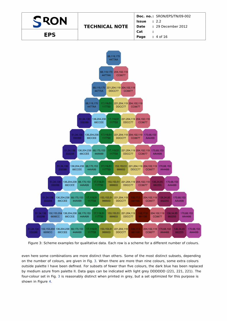
Figure 3: Scheme examples for qualitative data. Each row is a scheme for a different number of colours.

even here some combinations are more distinct than others. Some of the most distinct subsets, depending

on the number of colours, are given in Fig. 3. When there are more than nine colours, some extra colours

outside palette I have been defined. For subsets of fewer than five colours, the dark blue has been replaced

by medium azure from palette II. Data gaps can be indicated with light grey DDDDDD (221, 221, 221). The

four-colour set in Fig. 3 is reasonably distinct when printed in grey, but a set optimized for this purpose is

shown in Figure 4.

TECHNICAL NOTE

Doc. no. : SRON/EPS/TN/09-002

Issue : 2.2

Date : 29 December 2012

EPSCat :

Page : 5 of 16

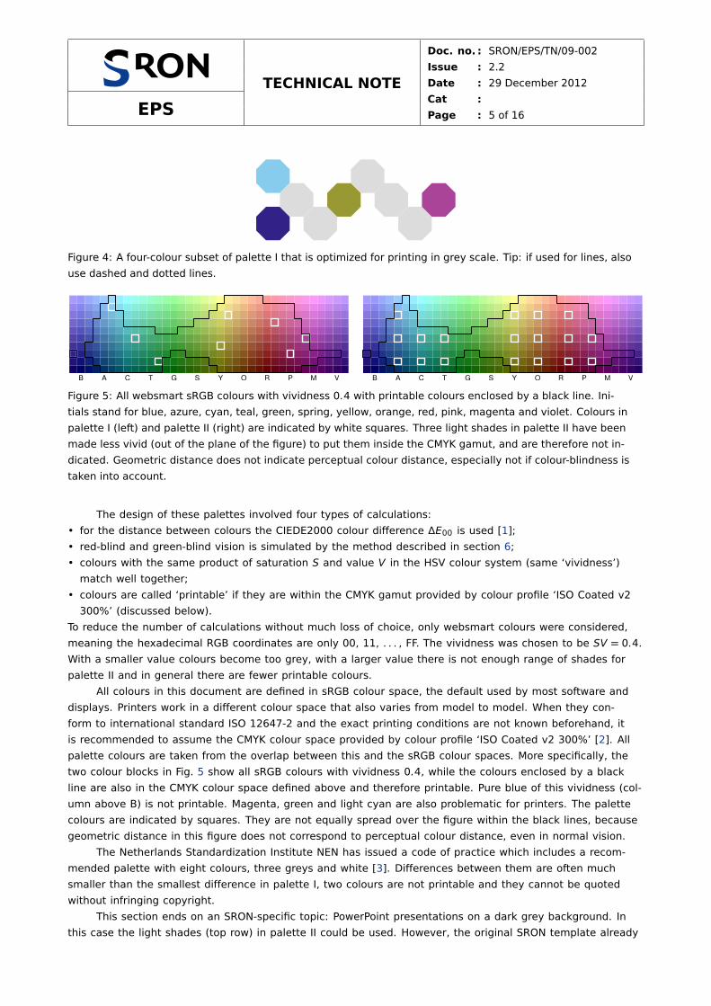
Figure 4: A four-colour subset of palette I that is optimized for printing in grey scale. Tip: if used for lines, also

use dashed and dotted lines.

B A C T G S Y O R P M V B A C T G S Y O R P M V

Figure 5: All websmart sRGB colours with vividness 0.4 with printable colours enclosed by a black line. Ini-

tials stand for blue, azure, cyan, teal, green, spring, yellow, orange, red, pink, magenta and violet. Colours in

palette I (left) and palette II (right) are indicated by white squares. Three light shades in palette II have been

made less vivid (out of the plane of the figure) to put them inside the CMYK gamut, and are therefore not in-

dicated. Geometric distance does not indicate perceptual colour distance, especially not if colour-blindness is

taken into account.

The design of these palettes involved four types of calculations:

• for the distance between colours the CIEDE2000 colour difference ΔE00 is used [1];

• red-blind and green-blind vision is simulated by the method described in section 6;

• colours with the same product of saturation S and value V in the HSV colour system (same ‘vividness’)

match well together;

• colours are called ‘printable’ if they are within the CMYK gamut provided by colour profile ‘ISO Coated v2

300%’ (discussed below).

To reduce the number of calculations without much loss of choice, only websmart colours were considered,

meaning the hexadecimal RGB coordinates are only 00, 11, . . . , FF. The vividness was chosen to be SV = 0.4.

With a smaller value colours become too grey, with a larger value there is not enough range of shades for

palette II and in general there are fewer printable colours.

All colours in this document are defined in sRGB colour space, the default used by most software and

displays. Printers work in a different colour space that also varies from model to model. When they con-

form to international standard ISO 12647-2 and the exact printing conditions are not known beforehand, it

is recommended to assume the CMYK colour space provided by colour profile ‘ISO Coated v2 300%’ [2]. All

palette colours are taken from the overlap between this and the sRGB colour spaces. More specifically, the

two colour blocks in Fig. 5 show all sRGB colours with vividness 0.4, while the colours enclosed by a black

line are also in the CMYK colour space defined above and therefore printable. Pure blue of this vividness (col-

umn above B) is not printable. Magenta, green and light cyan are also problematic for printers. The palette

colours are indicated by squares. They are not equally spread over the figure within the black lines, because

geometric distance in this figure does not correspond to perceptual colour distance, even in normal vision.

The Netherlands Standardization Institute NEN has issued a code of practice which includes a recom-

mended palette with eight colours, three greys and white [3]. Differences between them are often much

smaller than the smallest difference in palette I, two colours are not printable and they cannot be quoted

without infringing copyright.

This section ends on an SRON-specific topic: PowerPoint presentations on a dark grey background. In

this case the light shades (top row) in palette II could be used. However, the original SRON template already

TECHNICAL NOTE

Doc. no. : SRON/EPS/TN/09-002

Issue : 2.2

Date : 29 December 2012

EPSCat :

Page : 6 of 16

255,255,255

FFFFFF

255,255,204

FFFFCC

255,204,102

FFCC66

128,155,200

809BC8

100,194,4

64C204

255,102,102

FF6666

66,66,66

424242

Figure 6: SRON PowerPoint colours on a dark grey background, with the left four taken from the original tem-

plate. Colours from the top row in Fig. 2 also work on this background.

defines three colours: white for titles, light yellow for normal text and orange for highlighted text. If the light

blue from the footer is added, two extra hues are green and red. The complete palette optimized for projec-

tion is shown in Fig. 6. The red is rather pale, because it becomes darker on a projection screen. The green is

carefully chosen so it differs from orange in red-blind vision and differs from red in green-blind vision.

3 Best Colour Scheme for Different Data Types

A colour scheme should reflect the type of data shown. There are three basic types of data:

1. Qualitative data—nominal or categorical data, where magnitude differences are not relevant. This includes

text in presentations and lines in plots. Use palette I (Fig. 3) or different hues (colours from a row) in palette II

(Fig. 2).

2. Sequential data—data ordered from low to high.

255,247,188

FFF7BC

254,196,79

FEC44F

217,95,14

D95F0E

255,251,213

FFFBD5

254,217,142

FED98E

251,154,41

FB9A29

204,76,2

CC4C02

255,251,213

FFFBD5

254,217,142

FED98E

251,154,41

FB9A29

217,95,14

D95F0E

153,52,4

993404

255,251,213

FFFBD5

254,227,145

FEE391

254,196,79

FEC44F

251,154,41

FB9A29

217,95,14

D95F0E

153,52,4

993404

255,251,213

FFFBD5

254,227,145

FEE391

254,196,79

FEC44F

251,154,41

FB9A29

236,112,20

EC7014

204,76,2

CC4C02

140,45,4

8C2D04

255,255,229

FFFFE5

255,247,188

FFF7BC

254,227,145

FEE391

254,196,79

FEC44F

251,154,41

FB9A29

236,112,20

EC7014

204,76,2

CC4C02

140,45,4

8C2D04

255,255,229

FFFFE5

255,247,188

FFF7BC

254,227,145

FEE391

254,196,79

FEC44F

251,154,41

FB9A29

236,112,20

EC7014

204,76,2

CC4C02

153,52,4

993404

102,37,6

662506

Figure 7: Scheme for sequential data [4]. The smooth version at the bottom is produced with Eq. (1).

TECHNICAL NOTE

Doc. no. : SRON/EPS/TN/09-002

Issue : 2.2

Date : 29 December 2012

EPSCat :

Page : 7 of 16

153,199,236

99C7EC

255,250,210

FFFAD2

245,162,117

F5A275

0,139,206

008BCE

180,221,247

B4DDF7

249,189,126

F9BD7E

208,50,50

D03232

0,139,206

008BCE

180,221,247

B4DDF7

255,250,210

FFFAD2

249,189,126

F9BD7E

208,50,50

D03232

58,137,201

3A89C9

153,199,236

99C7EC

230,245,254

E6F5FE

255,227,170

FFE3AA

245,162,117

F5A275

210,77,62

D24D3E

58,137,201

3A89C9

153,199,236

99C7EC

230,245,254

E6F5FE

255,250,210

FFFAD2

255,227,170

FFE3AA

245,162,117

F5A275

210,77,62

D24D3E

58,137,201

3A89C9

119,183,229

77B7E5

180,221,247

B4DDF7

230,245,254

E6F5FE

255,227,170

FFE3AA

249,189,126

F9BD7E

237,135,94

ED875E

210,77,62

D24D3E

58,137,201

3A89C9

119,183,229

77B7E5

180,221,247

B4DDF7

230,245,254

E6F5FE

255,250,210

FFFAD2

255,227,170

FFE3AA

249,189,126

F9BD7E

237,135,94

ED875E

210,77,62

D24D3E

61,82,161

3D52A1

58,137,201

3A89C9

119,183,229

77B7E5

180,221,247

B4DDF7

230,245,254

E6F5FE

255,227,170

FFE3AA

249,189,126

F9BD7E

237,135,94

ED875E

210,77,62

D24D3E

174,28,62

AE1C3E

61,82,161

3D52A1

58,137,201

3A89C9

119,183,229

77B7E5

180,221,247

B4DDF7

230,245,254

E6F5FE

255,250,210

FFFAD2

255,227,170

FFE3AA

249,189,126

F9BD7E

237,135,94

ED875E

210,77,62

D24D3E

174,28,62

AE1C3E

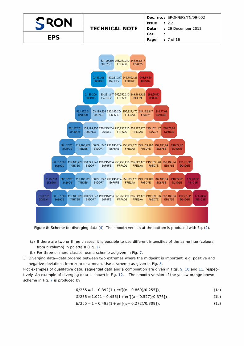
Figure 8: Scheme for diverging data [4]. The smooth version at the bottom is produced with Eq. (2).

(a) If there are two or three classes, it is possible to use different intensities of the same hue (colours

from a column) in palette II (Fig. 2).

(b) For three or more classes, use a scheme as given in Fig. 7.

3. Diverging data—data ordered between two extremes where the midpoint is important, e.g. positive and

negative deviations from zero or a mean. Use a scheme as given in Fig. 8.

Plot examples of qualitative data, sequential data and a combination are given in Figs. 9, 10 and 11, respec-

tively. An example of diverging data is shown in Fig. 12. The smooth version of the yellow-orange-brown

scheme in Fig. 7 is produced by

R/255 = 1− 0.392(1+ erf[(− 0.869)/0.255]) , (1a)

G/255 = 1.021− 0.456(1+ erf[(− 0.527)/0.376]) , (1b)

B/255 = 1− 0.493(1+ erf[(− 0.272)/0.309]) , (1c)

TECHNICAL NOTE

Doc. no. : SRON/EPS/TN/09-002

Issue : 2.2

Date : 29 December 2012

EPSCat :

Page : 8 of 16

-1.0 -0.5 0.0 0.5 1.0

-1.0

-0.5

0.0

0.5

1.0 blue

green

yellow

red

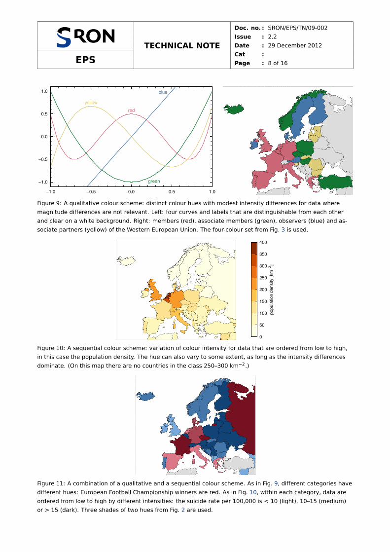
Figure 9: A qualitative colour scheme: distinct colour hues with modest intensity differences for data where

magnitude differences are not relevant. Left: four curves and labels that are distinguishable from each other

and clear on a white background. Right: members (red), associate members (green), observers (blue) and as-

sociate partners (yellow) of the Western European Union. The four-colour set from Fig. 3 is used.

0

50

100

150

200

250

300

350

400

po

pu

latio

nd

en

sity@k

m-

2D

Figure 10: A sequential colour scheme: variation of colour intensity for data that are ordered from low to high,

in this case the population density. The hue can also vary to some extent, as long as the intensity differences

dominate. (On this map there are no countries in the class 250–300 km−2.)

Figure 11: A combination of a qualitative and a sequential colour scheme. As in Fig. 9, different categories have

different hues: European Football Championship winners are red. As in Fig. 10, within each category, data are

ordered from low to high by different intensities: the suicide rate per 100,000 is < 10 (light), 10–15 (medium)

or > 15 (dark). Three shades of two hues from Fig. 2 are used.

TECHNICAL NOTE

Doc. no. : SRON/EPS/TN/09-002

Issue : 2.2

Date : 29 December 2012

EPSCat :

Page : 9 of 16

-100 -80 -60 -40 -20 0 20 40 60 80

geoid height @mD

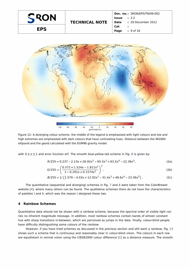
Figure 12: A diverging colour scheme: the middle of the legend is emphasized with light colours and low and

high extremes are emphasized with dark colours that have contrasting hues. Distance between the WGS84

ellipsoid and the geoid calculated with the EGM96 gravity model.

with 0 ≤ ≤ 1 and error function erf. The smooth blue-yellow-red scheme in Fig. 8 is given by:

R/255 = 0.237− 2.13+ 26.922 − 65.53 + 63.54 − 22.365 , (2a)

G/255 =

0.572+ 1.524− 1.8112

1− 0.291+ 0.15742

!2

, (2b)

B/255 = 1�

�

1.579− 4.03+ 12.922 − 31.43 + 48.64 − 23.365�

. (2c)

The quantitative (sequential and diverging) schemes in Fig. 7 and 8 were taken from the ColorBrewer

website [4], where many others can be found. The qualitative schemes there do not have the characteristics

of palettes I and II, which was the reason I designed these two.

4 Rainbow Schemes

Quantitative data should not be shown with a rainbow scheme, because the spectral order of visible light car-

ries no inherent magnitude message. In addition, most rainbow schemes contain bands of almost constant

hue with sharp transitions in-between, which are perceived as jumps in the data. Finally, colour-blind people

have difficulty distinguishing some colours of the rainbow.

However, if you have tried schemes as discussed in the previous section and still want a rainbow, Fig. 13

shows such a scheme that is continuous and reasonably clear in colour-blind vision. The colours in each row

are equidistant in normal vision using the CIEDE2000 colour difference [1] as a distance measure. The smooth

TECHNICAL NOTE

Doc. no. : SRON/EPS/TN/09-002

Issue : 2.2

Date : 29 December 2012

EPSCat :

Page : 10 of 16

64,64,150

404096

87,163,173

57A3AD

222,167,58

DEA73A

217,33,32

D92120

64,64,150

404096

82,157,183

529DB7

125,184,116

7DB874

227,156,55

E39C37

217,33,32

D92120

64,64,150

404096

73,140,194

498CC2

99,173,153

63AD99

190,188,72

BEBC48

230,139,51

E68B33

217,33,32

D92120

120,28,129

781C81

63,96,174

3F60AE

83,158,182

539EB6

109,179,136

6DB388

202,184,67

CAB843

231,133,50

E78532

217,33,32

D92120

120,28,129

781C81

63,86,167

3F56A7

75,145,192

4B91C0

95,170,159

5FAA9F

145,189,97

91BD61

216,175,61

D8AF3D

231,124,48

E77C30

217,33,32

D92120

120,28,129

781C81

63,78,161

3F4EA1

70,131,193

4683C1

87,163,173

57A3AD

109,179,136

6DB388

177,190,78

B1BE4E

223,165,58

DFA53A

231,116,47

E7742F

217,33,32

D92120

120,28,129

781C81

63,71,155

3F479B

66,119,189

4277BD

82,157,183

529DB7

98,172,155

62AC9B

134,187,106

86BB6A

199,185,68

C7B944

227,156,55

E39C37

231,109,46

E76D2E

217,33,32

D92120

120,28,129

781C81

64,64,150

404096

65,108,183

416CB7

77,149,190

4D95BE

91,167,167

5BA7A7

110,179,135

6EB387

161,190,86

A1BE56

211,179,63

D3B33F

229,148,53

E59435

230,104,45

E6682D

217,33,32

D92120

120,28,129

781C81

65,59,147

413B93

64,101,177

4065B1

72,139,194

488BC2

85,161,177

55A1B1

99,173,153

63AD99

127,185,114

7FB972

181,189,76

B5BD4C

217,173,60

D9AD3C

230,142,52

E68E34

230,100,44

E6642C

217,33,32

D92120

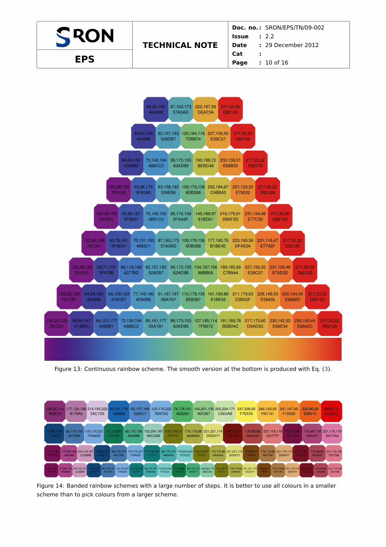
Figure 13: Continuous rainbow scheme. The smooth version at the bottom is produced with Eq. (3).

136,46,114

882E72

177,120,166

B178A6

214,193,222

D6C1DE

25,101,176

1965B0

82,137,199

5289C7

123,175,222

7BAFDE

78,178,101

4EB265

144,201,135

90C987

202,224,171

CAE0AB

247,238,85

F7EE55

246,193,65

F6C141

241,147,45

F1932D

232,96,28

E8601C

220,5,12

DC050C

17,68,119

114477

68,119,170

4477AA

119,170,221

77AADD

17,119,85

117755

68,170,136

44AA88

153,204,187

99CCBB

119,119,17

777711

170,170,68

AAAA44

221,221,119

DDDD77

119,17,17

771111

170,68,68

AA4444

221,119,119

DD7777

119,17,68

771144

170,68,119

AA4477

221,119,170

DD77AA

119,17,85

771155

170,68,136

AA4488

204,153,187

CC99BB

17,68,119

114477

68,119,170

4477AA

119,170,221

77AADD

17,119,119

117777

68,170,170

44AAAA

119,204,204

77CCCC

119,119,17

777711

170,170,68

AAAA44

221,221,119

DDDD77

119,68,17

774411

170,119,68

AA7744

221,170,119

DDAA77

119,17,34

771122

170,68,85

AA4455

221,119,136

DD7788

119,17,85

771155

170,68,136

AA4488

204,153,187

CC99BB

17,68,119

114477

68,119,170

4477AA

119,170,221

77AADD

17,119,119

117777

68,170,170

44AAAA

119,204,204

77CCCC

17,119,68

117744

68,170,119

44AA77

136,204,170

88CCAA

119,119,17

777711

170,170,68

AAAA44

221,221,119

DDDD77

119,68,17

774411

170,119,68

AA7744

221,170,119

DDAA77

119,17,34

771122

170,68,85

AA4455

221,119,136

DD7788

Figure 14: Banded rainbow schemes with a large number of steps. It is better to use all colours in a smaller

scheme than to pick colours from a larger scheme.

TECHNICAL NOTE

Doc. no. : SRON/EPS/TN/09-002

Issue : 2.2

Date : 29 December 2012

EPSCat :

Page : 11 of 16

-100 -50 0 50 100 150

longitude @degreesD

-60

-40

-20

0

20

latitu

de@d

eg

ree

sD

0.6 0.8 1.0 1.2 1.4 1.6 1.8 2.0 2.2 2.4 2.6 2.8 3.0

1018 molecules�cm2

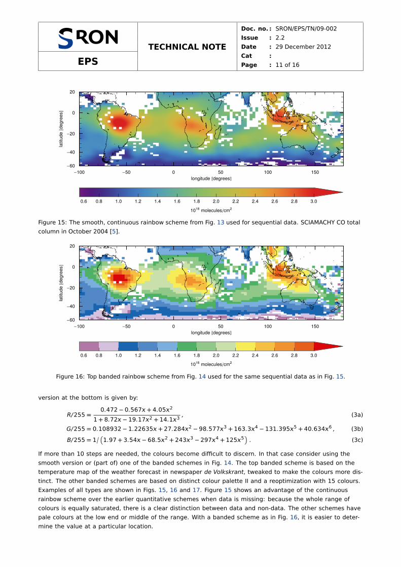
Figure 15: The smooth, continuous rainbow scheme from Fig. 13 used for sequential data. SCIAMACHY CO total

column in October 2004 [5].

-100 -50 0 50 100 150

longitude @degreesD

-60

-40

-20

0

20

latitu

de@d

eg

ree

sD

0.6 0.8 1.0 1.2 1.4 1.6 1.8 2.0 2.2 2.4 2.6 2.8 3.0

1018 molecules�cm2

Figure 16: Top banded rainbow scheme from Fig. 14 used for the same sequential data as in Fig. 15.

version at the bottom is given by:

R/255 =0.472− 0.567+ 4.052

1+ 8.72− 19.172 + 14.13, (3a)

G/255 = 0.108932− 1.22635+ 27.2842 − 98.5773 + 163.34 − 131.3955 + 40.6346 , (3b)

B/255 = 1�

�

1.97+ 3.54− 68.52 + 2433 − 2974 + 1255�

. (3c)

If more than 10 steps are needed, the colours become difficult to discern. In that case consider using the

smooth version or (part of) one of the banded schemes in Fig. 14. The top banded scheme is based on the

temperature map of the weather forecast in newspaper de Volkskrant, tweaked to make the colours more dis-

tinct. The other banded schemes are based on distinct colour palette II and a reoptimization with 15 colours.

Examples of all types are shown in Figs. 15, 16 and 17. Figure 15 shows an advantage of the continuous

rainbow scheme over the earlier quantitative schemes when data is missing: because the whole range of

colours is equally saturated, there is a clear distinction between data and non-data. The other schemes have

pale colours at the low end or middle of the range. With a banded scheme as in Fig. 16, it is easier to deter-

mine the value at a particular location.

TECHNICAL NOTE

Doc. no. : SRON/EPS/TN/09-002

Issue : 2.2

Date : 29 December 2012

EPSCat :

Page : 12 of 16

0 0.1 0.2 0.3 0.4 0.5 0.6 0.7 0.8

albedo

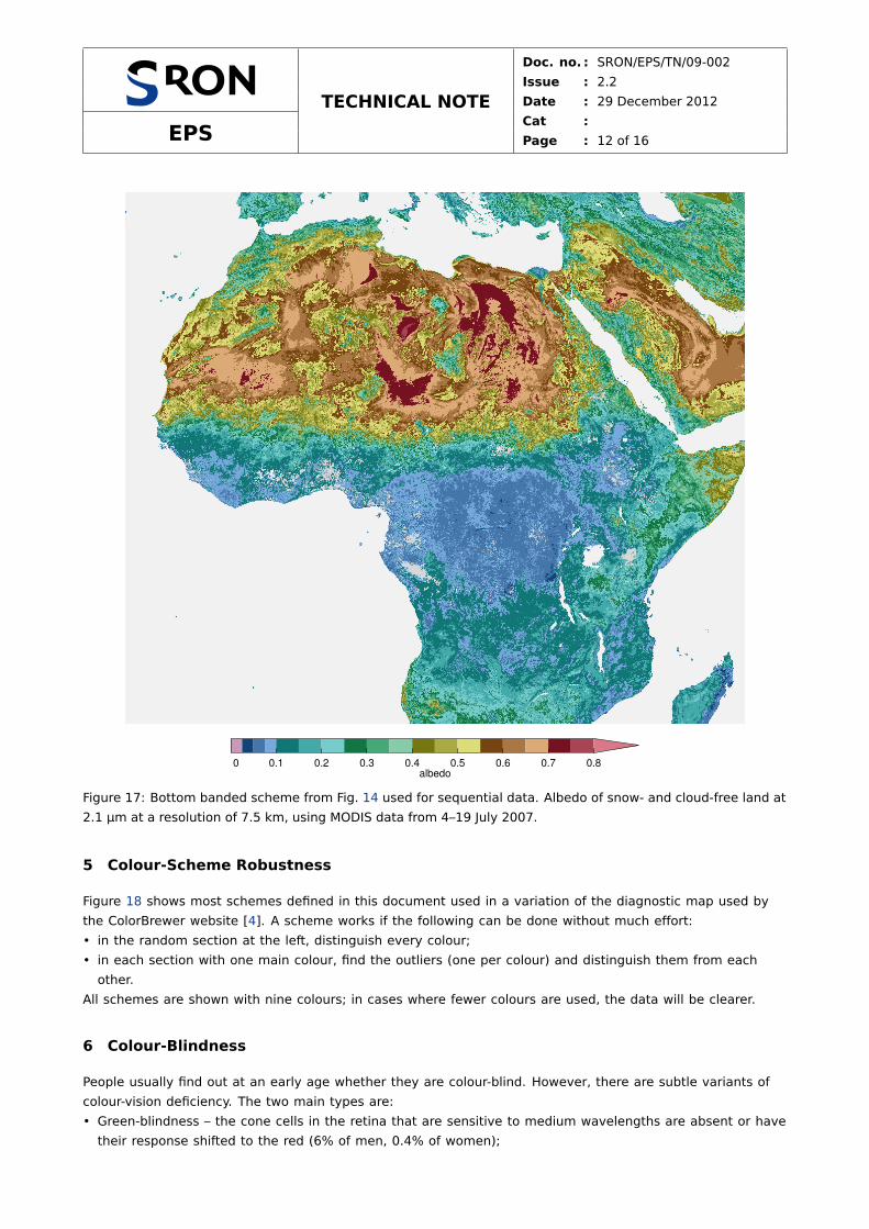
Figure 17: Bottom banded scheme from Fig. 14 used for sequential data. Albedo of snow- and cloud-free land at

2.1 µm at a resolution of 7.5 km, using MODIS data from 4–19 July 2007.

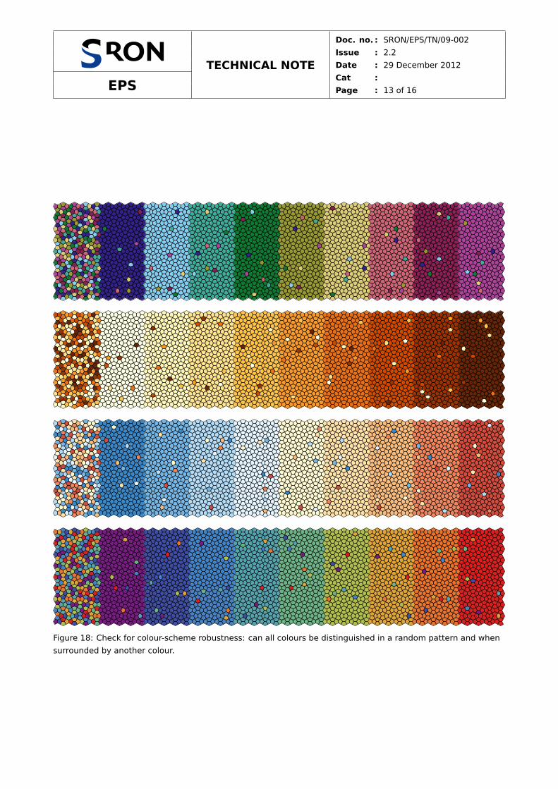
5 Colour-Scheme Robustness

Figure 18 shows most schemes defined in this document used in a variation of the diagnostic map used by

the ColorBrewer website [4]. A scheme works if the following can be done without much effort:

• in the random section at the left, distinguish every colour;

• in each section with one main colour, find the outliers (one per colour) and distinguish them from each

other.

All schemes are shown with nine colours; in cases where fewer colours are used, the data will be clearer.

6 Colour-Blindness

People usually find out at an early age whether they are colour-blind. However, there are subtle variants of

colour-vision deficiency. The two main types are:

• Green-blindness – the cone cells in the retina that are sensitive to medium wavelengths are absent or have

their response shifted to the red (6% of men, 0.4% of women);

TECHNICAL NOTE

Doc. no. : SRON/EPS/TN/09-002

Issue : 2.2

Date : 29 December 2012

EPSCat :

Page : 13 of 16

Figure 18: Check for colour-scheme robustness: can all colours be distinguished in a random pattern and when

surrounded by another colour.

TECHNICAL NOTE

Doc. no. : SRON/EPS/TN/09-002

Issue : 2.2

Date : 29 December 2012

EPSCat :

Page : 14 of 16

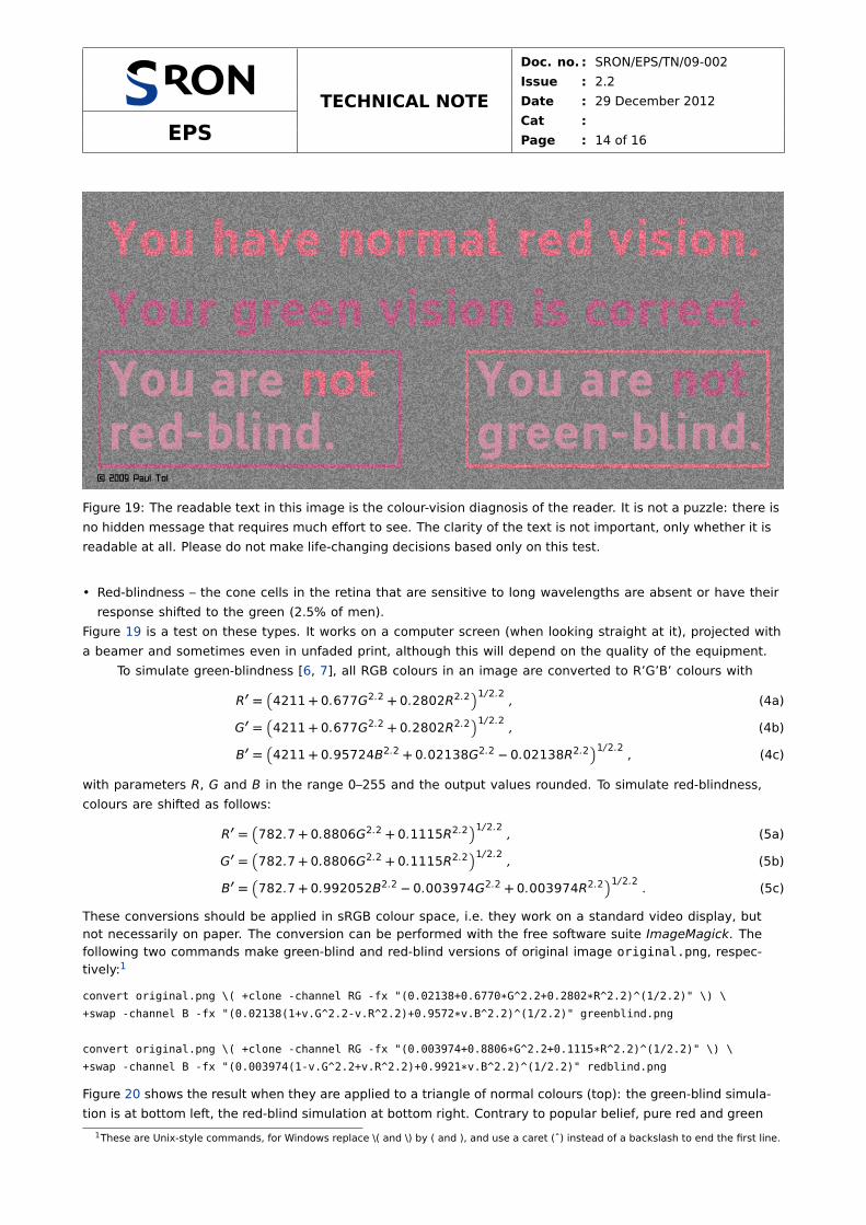
Figure 19: The readable text in this image is the colour-vision diagnosis of the reader. It is not a puzzle: there is

no hidden message that requires much effort to see. The clarity of the text is not important, only whether it is

readable at all. Please do not make life-changing decisions based only on this test.

• Red-blindness – the cone cells in the retina that are sensitive to long wavelengths are absent or have their

response shifted to the green (2.5% of men).

Figure 19 is a test on these types. It works on a computer screen (when looking straight at it), projected with

a beamer and sometimes even in unfaded print, although this will depend on the quality of the equipment.

To simulate green-blindness [6, 7], all RGB colours in an image are converted to R’G’B’ colours with

R′ =�

4211+ 0.677G2.2 + 0.2802R2.2�1/2.2

, (4a)

G′ =�

4211+ 0.677G2.2 + 0.2802R2.2�1/2.2

, (4b)

B′ =�

4211+ 0.95724B2.2 + 0.02138G2.2 − 0.02138R2.2�1/2.2

, (4c)

with parameters R, G and B in the range 0–255 and the output values rounded. To simulate red-blindness,

colours are shifted as follows:

R′ =�

782.7+ 0.8806G2.2 + 0.1115R2.2�1/2.2

, (5a)

G′ =�

782.7+ 0.8806G2.2 + 0.1115R2.2�1/2.2

, (5b)

B′ =�

782.7+ 0.992052B2.2 − 0.003974G2.2 + 0.003974R2.2�1/2.2

. (5c)

These conversions should be applied in sRGB colour space, i.e. they work on a standard video display, but

not necessarily on paper. The conversion can be performed with the free software suite ImageMagick. The

following two commands make green-blind and red-blind versions of original image original.png, respec-

tively:1

convert original.png \( +clone -channel RG -fx "(0.02138+0.6770*G^2.2+0.2802*R^2.2)^(1/2.2)" \) \

+swap -channel B -fx "(0.02138(1+v.G^2.2-v.R^2.2)+0.9572*v.B^2.2)^(1/2.2)" greenblind.png

convert original.png \( +clone -channel RG -fx "(0.003974+0.8806*G^2.2+0.1115*R^2.2)^(1/2.2)" \) \

+swap -channel B -fx "(0.003974(1-v.G^2.2+v.R^2.2)+0.9921*v.B^2.2)^(1/2.2)" redblind.png

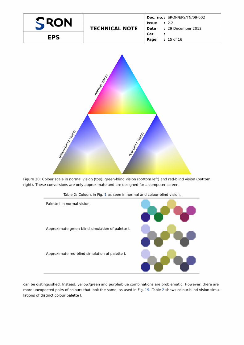
Figure 20 shows the result when they are applied to a triangle of normal colours (top): the green-blind simula-

tion is at bottom left, the red-blind simulation at bottom right. Contrary to popular belief, pure red and green

1These are Unix-style commands, for Windows replace \( and \) by ( and ), and use a caret (ˆ) instead of a backslash to end the first line.

TECHNICAL NOTE

Doc. no. : SRON/EPS/TN/09-002

Issue : 2.2

Date : 29 December 2012

EPSCat :

Page : 15 of 16

gree

n-bl

ind

visi

on

red-

blin

dvi

sion

norm

alvi

sion

Figure 20: Colour scale in normal vision (top), green-blind vision (bottom left) and red-blind vision (bottom

right). These conversions are only approximate and are designed for a computer screen.

Table 2: Colours in Fig. 1 as seen in normal and colour-blind vision.

Palette I in normal vision.

Approximate green-blind simulation of palette I.

Approximate red-blind simulation of palette I.

can be distinguished. Instead, yellow/green and purple/blue combinations are problematic. However, there are

more unexpected pairs of colours that look the same, as used in Fig. 19. Table 2 shows colour-blind vision simu-

lations of distinct colour palette I.

TECHNICAL NOTE

Doc. no. : SRON/EPS/TN/09-002

Issue : 2.2

Date : 29 December 2012

EPSCat :

Page : 16 of 16

Reference Documents

[1] Gaurav Sharma, Wencheng Wu, and Edul N. Dalal. The CIEDE2000 color-difference formula: implementation

notes, supplementary test data, and mathematical observations. Color Research and Application, 30:21–30,

2005. http://www.ece.rochester.edu/~gsharma/ciede2000/ciede2000noteCRNA.pdf.

[2] Olaf Drümmer. ECI offset profiles, 2009. http://www.eci.org/doku.php?id=en:colorstandards:offset.

[3] Normcommissie ‘Ergonomie van de fysische werkomgeving’ with Buro Blind Color. Functional use of

colour—accommodating colour vision disorders. Code of practice NPR 7022, Netherlands Standardization

Institute, Delft, April 2006.

[4] Cynthia A. Brewer. ColorBrewer, a web tool for selecting colors for maps, 2009. http://colorbrewer2.org.

[5] A.M.S. Gloudemans, M.C. Krol, J.F. Meirink, A.T.J. de Laat, G.R. van der Werf, H. Schrijver, M.M.P. van den

Broek, and I. Aben. Evidence for long-range transport of carbon monoxide in the southern hemisphere from

SCIAMACHY observations. Geophysical Research Letters, 33:L16807, 2006.

[6] Françoise Viénot, Hans Brettel, and John D. Mollon. Digital video colourmaps for checking the legibility of

displays by dichromats. Color Research and Application, 24:243–252, 1999.

[7] Hans Brettel, Françoise Viénot, and John D. Mollon. Computerized simulation of color appearance for dichro-

mats. Journal of the Optical Society of America A, 14:2647–2655, 1997.