equations of continuity. outline 1.time derivatives & vector notation 2.differential equations...
TRANSCRIPT

Equations of Continuity

Outline
1.Time Derivatives & Vector Notation
2.Differential Equations of Continuity
3.Momentum Transfer Equations
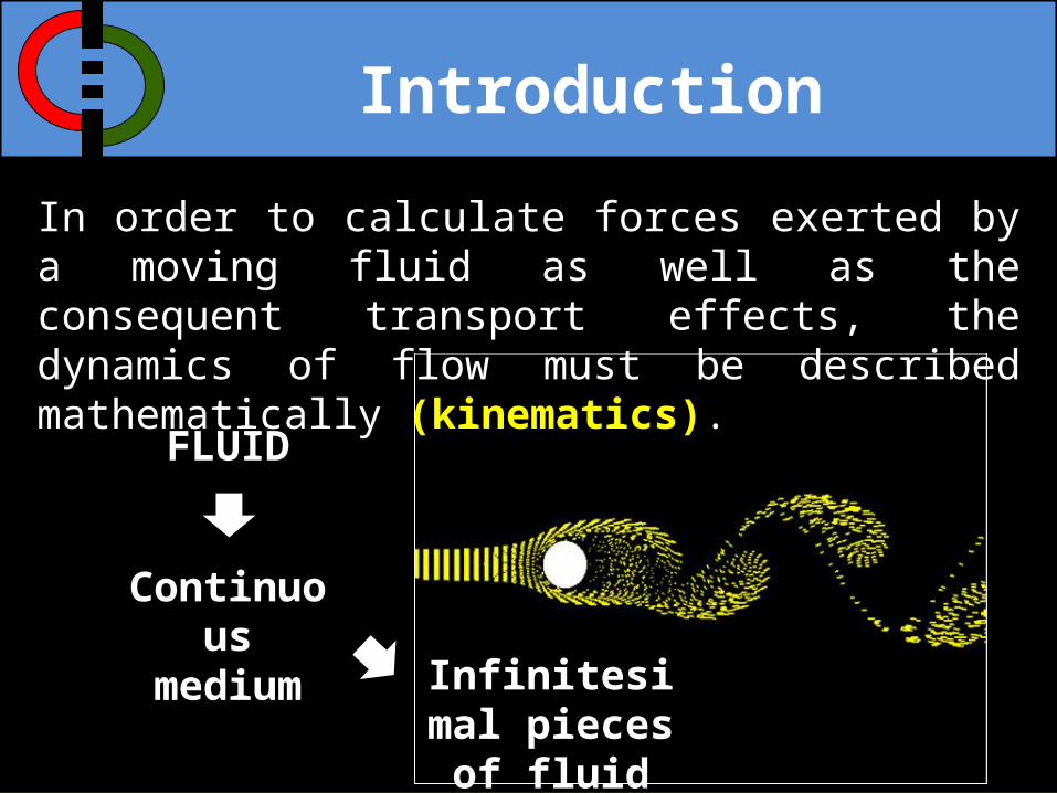
Introduction
FLUID
In order to calculate forces exerted by a moving fluid as well as the consequent transport effects, the dynamics of flow must be described mathematically (kinematics).
Continuousmedium
Infinitesimal pieces of fluid
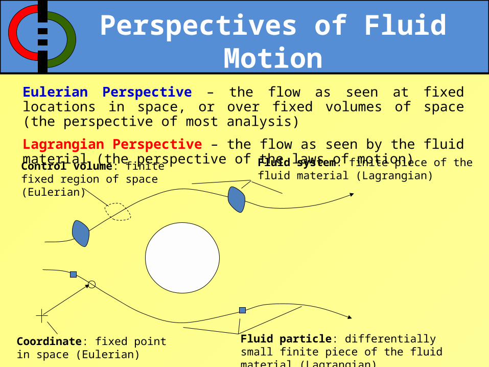
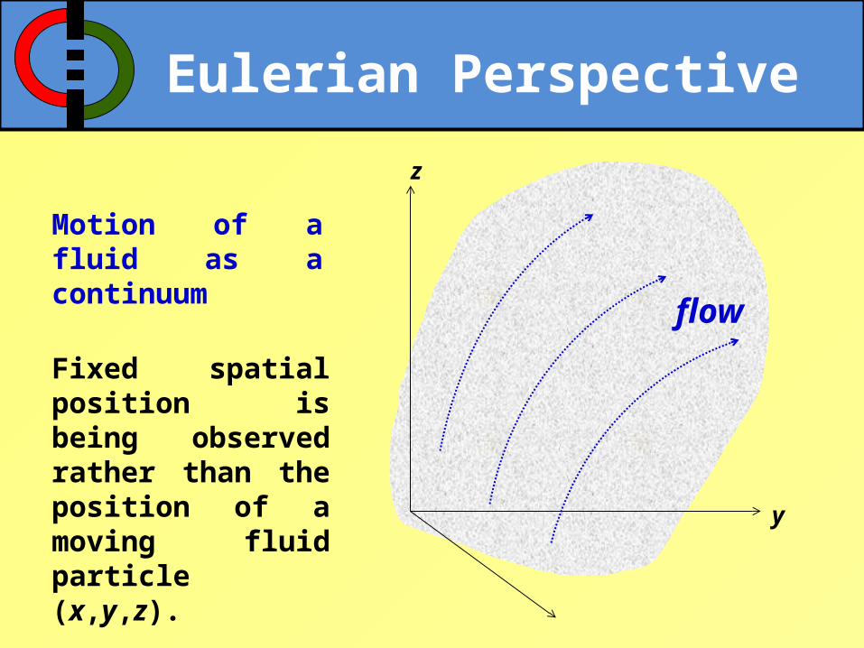
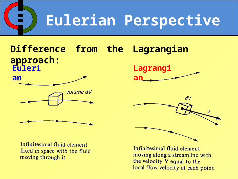
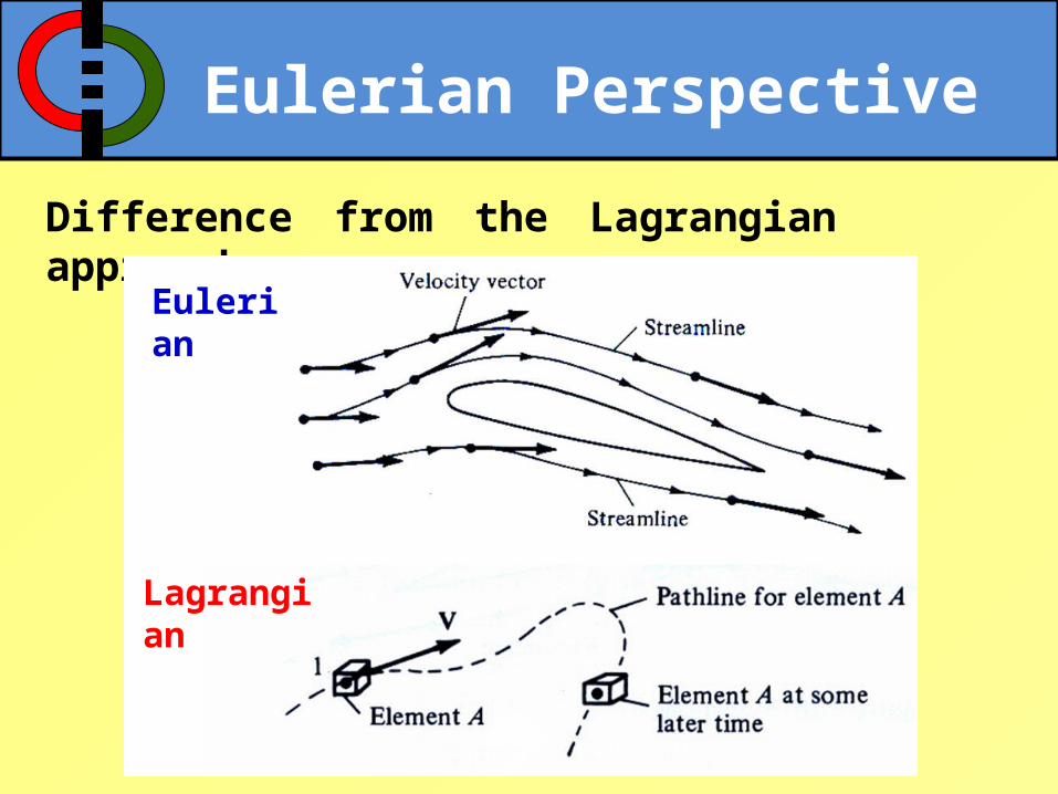
Eulerian Perspective – the flow as seen at fixed locations in space, or over fixed volumes of space (the perspective of most analysis)
Lagrangian Perspective – the flow as seen by the fluid material (the perspective of the laws of motion)
Control volume: finite fixed region of space (Eulerian)
Coordinate: fixed point in space (Eulerian)
Fluid system: finite piece of the fluid material (Lagrangian)
Fluid particle: differentially small finite piece of the fluid material (Lagrangian)
Perspectives of Fluid Motion

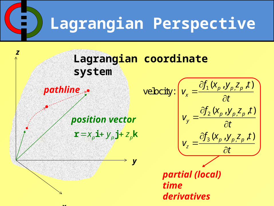
Lagrangian Perspective
The motion of a fluid particle is relative to a specific initial position in space at an initial time.
1 , 2 , 3 ,
position:
( , , ) ( , , ) ( , , ) p p p p p p p p px f x y z t y f x y z t z f x y z t
Lagrangian Perspective
x
y
zLagrangian coordinate system
pathline
position vector
p p px y zr i j k
1 ,
2 ,
3 ,
( , , )velocity:
( , , )
( , , )
p p px
p p py
p p pz
f x y z tv
tf x y z t
vt
f x y z tv
t
partial (local) time derivatives

Lagrangian Perspective
x
y
z
t = t1 t = t2y
xz
1 1 1, 1
2 1 1, 1
3 1 1, 1
position 1:
( , , )
( , , )
( , , )
p p p
p p p
p p p
x f x y z t
y f x y z t
z f x y z t
1 2 2, 2
2 2 2, 2
3 2 2, 2
position 2:
( , , )
( , , )
( , , )
p p p
p p p
p p p
x f x y z t
y f x y z t
z f x y z t
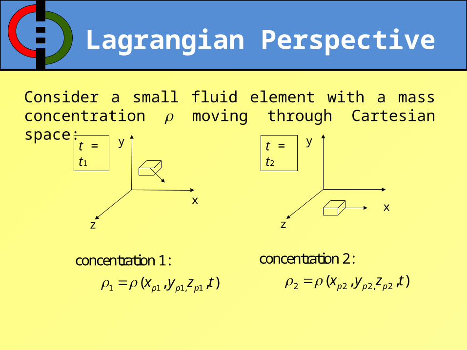
Consider a small fluid element with a mass concentration moving through Cartesian space:
Lagrangian Perspective
x
y
z
t = t1 t = t2y
xz
Consider a small fluid element with a mass concentration moving through Cartesian space:
1 1 1, 1
concentration 1:
( , , ) p p px y z t 2 2 2, 2
concentration 2:
( , , ) p p px y z t
Lagrangian Perspective
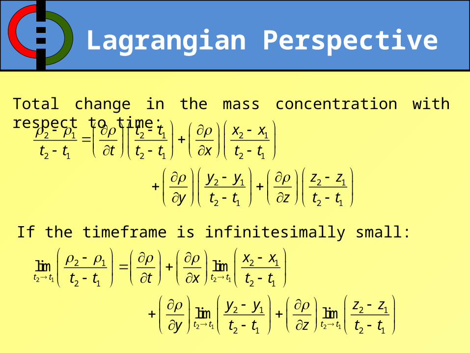
Total change in the mass concentration with respect to time:
2 1 2 1 2 1
2 1 2 1 2 1
2 1 2 1
2 1 2 1
t t x x
t t t t t x t t
y y z z
y t t z t t
If the timeframe is infinitesimally small:
2 1 2 1
2 1 2 1
2 1 2 1
2 1 2 1
2 1 2 1
2 1 2 1
lim lim
lim lim
t t t t
t t t t
x x
t t t x t t
y y z z
y t t z t t

Lagrangian Perspective
Total Time Derivative
d x y z
dt t x t y t z t
x y z
Dv v v
Dt t x y z
local derivative convective derivative
Substantial Time Derivative
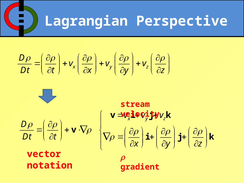
Lagrangian Perspective
x y z
Dv v v
Dt t x y z
D
Dt tv
x y zv v v
x y z
v i j k
i j k
vector notation
stream velocity
gradient
Lagrangian Perspective
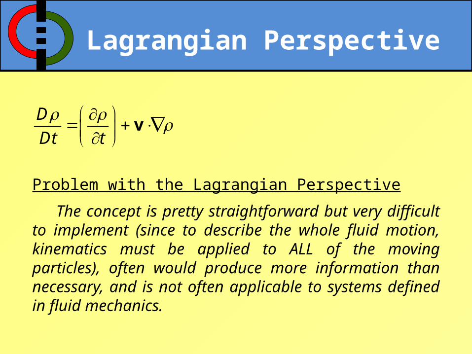
Problem with the Lagrangian Perspective
The concept is pretty straightforward but very difficult to implement (since to describe the whole fluid motion, kinematics must be applied to ALL of the moving particles), often would produce more information than necessary, and is not often applicable to systems defined in fluid mechanics.
D
Dt tv
Eulerian Perspective
flow
x
y
z
Motion of a fluid as a continuum
Fixed spatial position is being observed rather than the position of a moving fluid particle (x,y,z).

Eulerian Perspective
flow
x
y
z
Motion of a fluid as a continuum
Velocity expressed as a function of time t and spatial position (x, y, z)
Eulerian coordinate system
Eulerian Perspective
Difference from the Lagrangian approach:
Eulerian Lagrangian
Eulerian Perspective
Difference from the Lagrangian approach:
Eulerian
Lagrangian

Outline
1.Time Derivatives & Vector Notation
2.Differential Equations of Continuity
3.Momentum Transfer Equations
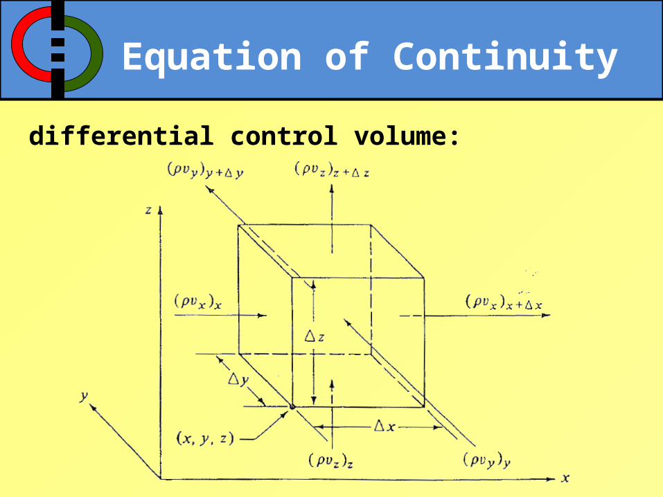
Equation of Continuity
differential control volume:
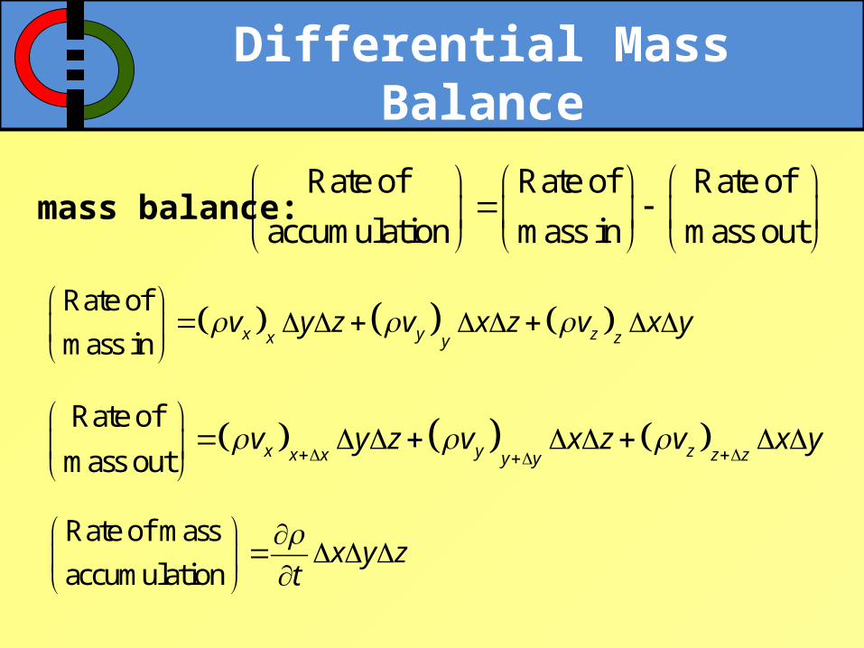
Differential Mass Balance
Rate of Rate of Rate of
accumulation mass in mass out
mass balance:
Rate of
mass in
x y zx zyv y z v x z v x y
Rate of
mass out
x y zx x z zy yv y z v x z v x y
Rate of mass
accumulationx y z
t

Differential Mass Balance
Substituting:
x y zx zy
x y zx x z zy y
x y z v y z v x z v x yt
v y z v x z v x y
Rearranging:
x xx x x
y yy y y
z zz z z
x y z v v y zt
v v x z
v v x y
Differential Equation of Continuity
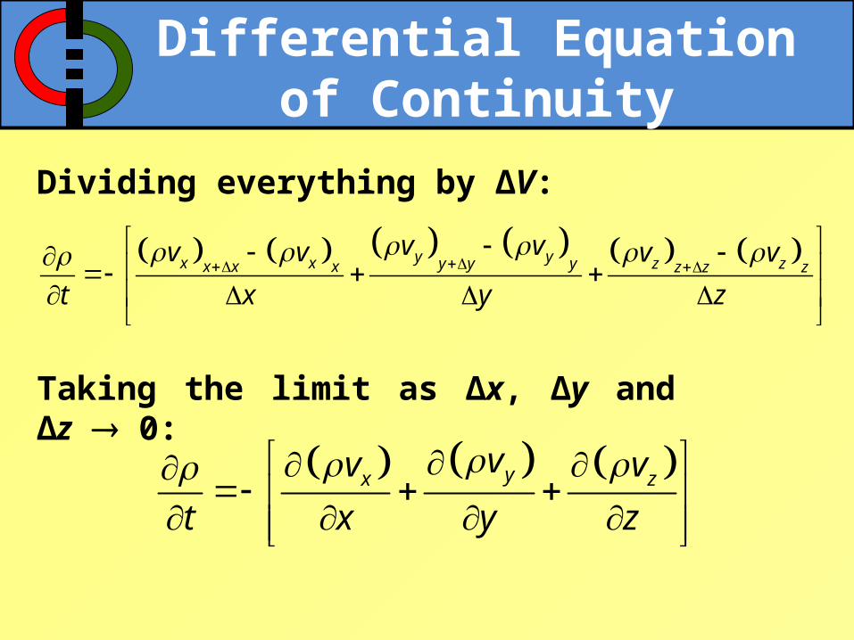
Dividing everything by ΔV:
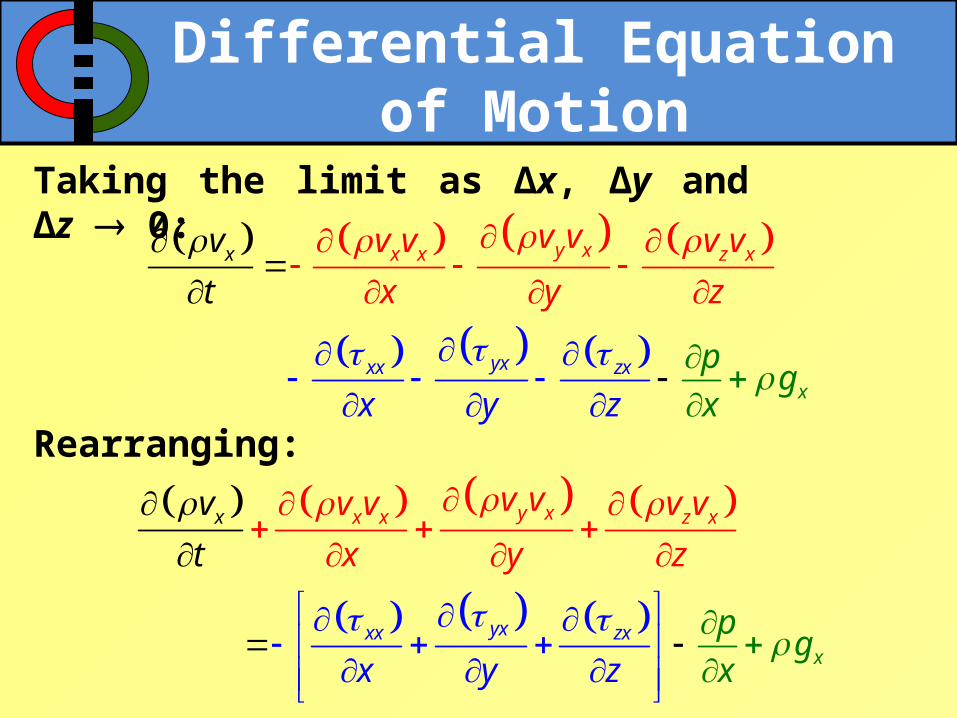
Taking the limit as ∆x, ∆y and ∆z 0:
y yx x z zy y yx x x z z zv vv v v v
t x y z
yx zvv v
t x y z

Differential Equation of Continuity
yx zvv v
t x y z
v
divergence of mass velocity vector (v)
Partial differentiation:
yx zx y z
vv vv v v
t x y z x y z
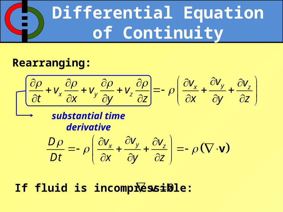
Differential Equation of Continuity
Rearranging:
yx zx y z
vv vv v v
t x y z x y z
substantial time derivative
yx zvv vD
Dt x y zv
If fluid is incompressible: 0 v
Differential Equation of Continuity
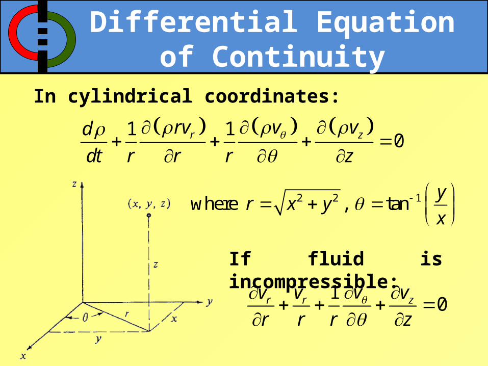
In cylindrical coordinates:
1 10
r zrv v vd
dt r r r z
2 2 1where , tan y
r x yx
If fluid is incompressible:
10
r r zvv v v
r r r z

Outline
1.Time Derivatives & Vector Notation
2.Differential Equations of Continuity
3.Momentum Transfer Equations
Differential Equations of Motion
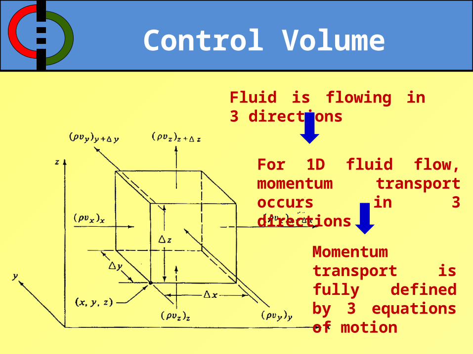
Control Volume
For 1D fluid flow, momentum transport occurs in 3 directions
Fluid is flowing in 3 directions
Momentum transport is fully defined by 3 equations of motion

Momentum Balance
Sum of forcesRate of Rate of Rate of
acting in accumulation momentum in momentum out
the systemx x xx
convective
Rate of Rate of
momentum in momentum out
Rate of Rate of
momentum in momentum out
Rate of
momentum in
x x
x x
molecular
Rate of
momentum outx x
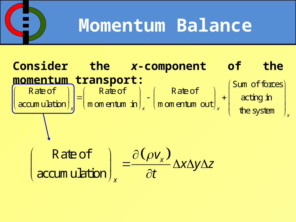
Consider the x-component of the momentum transport:

Momentum Balance
convective
Rate of Rate of
momentum in momentum out
x x x xx x
x x
xv v v v y z
y x y xy y y
z x z xz z z
v v v v x z
v v v v x y
Due to convective transport:
Momentum Balance
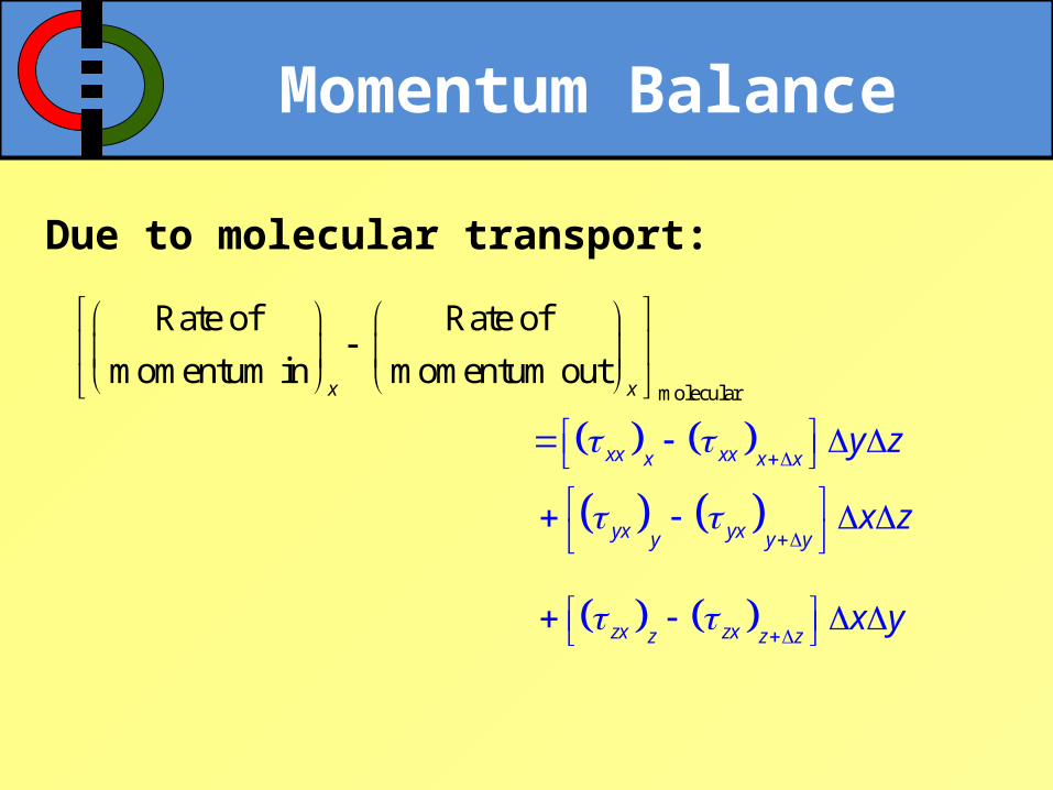
molecular
Rate of Rate of
momentum in momentum out
xx xxx x x
yx yx y
x
y
x
y z
y
zx zxz z z
x z
x y
Due to molecular transport:

Momentum Balance
Sum of forcesRate of Rate of Rate of
acting in accumulation momentum in momentum out
the systemx x xx
Sum of forces
acting in
the systemx x x x
x
p p y z g x y z
Consider the x-component of the momentum transport:
Momentum Balance
Sum of forcesRate of Rate of Rate of
acting in accumulation momentum in momentum out
the systemx x xx
Rate of
accumulationx
x
vx y z
t
Consider the x-component of the momentum transport:

Differential Momentum Balance
Substituting:
x x x xx x x
y x y xy y y
z x
xx xxx x
x
z
x
xz z z
y z
vx y z
tv v v v y z
v v v v x z
v v v v x y
yx yxy y y
z
x x x x
x zxz z z
x z
x
p p y z g x y z
y
Differential Momentum Balance
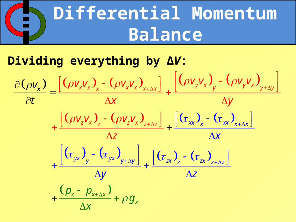
Dividing everything by ΔV:
y x y xx x x x y y yx x x
z x xx xxx x xz
yx yx zx zxy y y z z z
x x
xz z
x
z
xx
p pg
x
x
y
v v v vv v v v
x y
v v
z
t
v v
z
v
Differential Equation of Motion
Taking the limit as ∆x, ∆y and ∆z 0:
y xx x
yxxx z
z x
xx
x
x y z
pg
x
v vv v v v
x y z
v
t
Rearranging:
y xx x
x
yxxx x
z
z
xxv vv v v vv
t
x yg
x y
p
z
z x

Differential Momentum Balance
For the convective terms:
y xx x z x
yx zx x xx y z x
v vv v v v
x y z
vv vv v vv v v v
x y z x y z
For the accumulation term:
x xx
yx x zx x y z
v vv
t t t
vv v vv v v v
t x y z x y z

Differential Equation of Motion
Substituting:
x x x
yx x z
x
x x
y z
yx z
yxxx z
y
x
z
xx
vv v
v v vv v v
x y z
vv vv
x y z
vv v v v
t x y z x
x y z
z
g
y
p
x
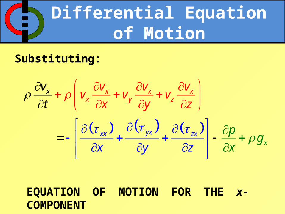
Differential Equation of Motion
x xx xx y
yxxx zxx
z
v v vv v v
x y z
v
gx y x
t
z
p
EQUATION OF MOTION FOR THE x-COMPONENT
Substituting:
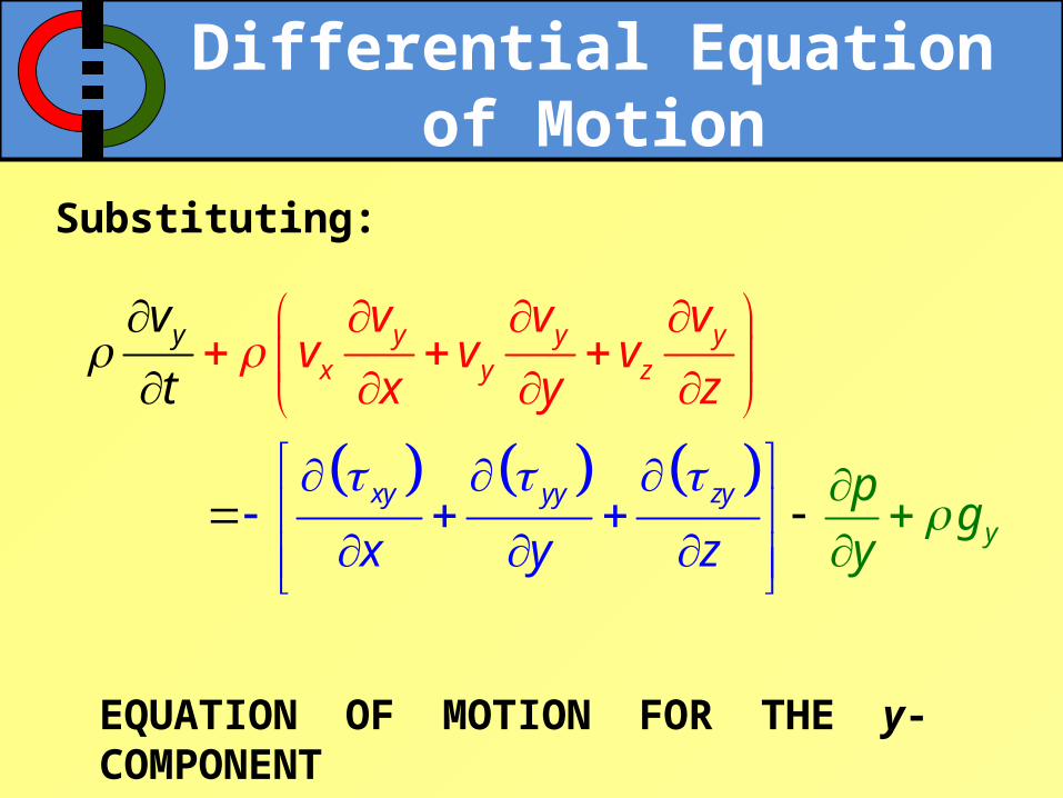
Differential Equation of Motion
Substituting:
EQUATION OF MOTION FOR THE y-COMPONENT
y yy yx y
xy yy zy
y
z
v v vv v v
x y z
xg
v
y z
t
p
y

Differential Equation of Motion
Substituting:
EQUATION OF MOTION FOR THE z-COMPONENT
z zz zx y
yzxz zzz
z
v v vv v v
x y z
v
gx y z
t
z
p

Differential Equation of Motion
Substantial time derivatives:
yxxx zxxx
xy yy zyyy
yzxz zzzz
Dv pg
Dt x y z x
Dv pg
Dt x y z y
Dv pg
Dt x y z z

Differential Equation of Motion
In vector-matrix notation:
yxxx zx
x xxy yy zy
y y
z z
yzxz zz
px y z
xv gD pv g
Dt x y z yv g
p
zx y z
Dp
Dt
vg
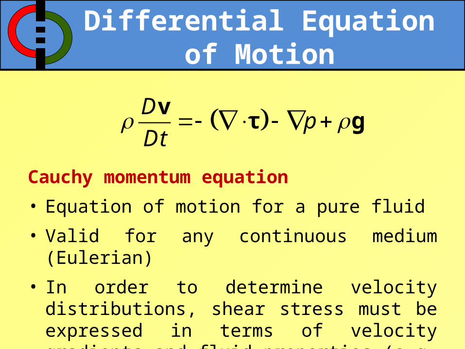
Differential Equation of Motion
Cauchy momentum equation
• Equation of motion for a pure fluid
• Valid for any continuous medium (Eulerian)
• In order to determine velocity distributions, shear stress must be expressed in terms of velocity gradients and fluid properties (e.g. Newton’s law)
Dp
Dt
vτ g
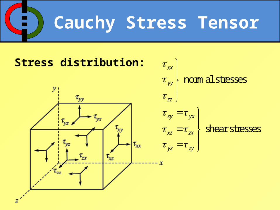
Cauchy Stress Tensor
Stress distribution: normal stresses
shear stresses
xx
yy
zz
xy yx
xz zx
yz zy
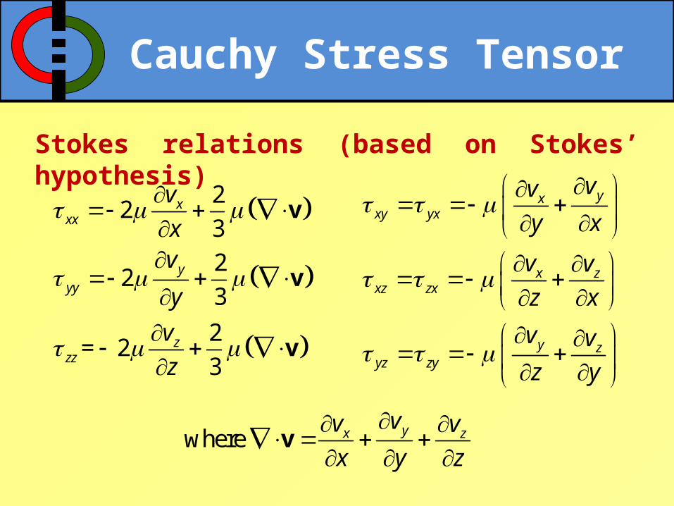
Cauchy Stress Tensor
Stokes relations (based on Stokes’ hypothesis)
22
3
22
3
2= 2
3
xxx
yyy
zzz
v
xv
y
v
z
v
v
v
yxxy yx
x zxz zx
y zyz zy
vv
y x
v v
z x
v v
z y
where yx zvv v
x y z
v

Navier-Stokes Equations

Assumptions
1. Newtonian fluid
2. Obeys Stokes’ hypothesis
3. Continuum
4. Isotropic viscosity
5. Constant density
Divergence of the stream velocity is zero

Navier-Stokes Equations
Applying the Stokes relations per component:
2 2 2
2 2 2
2 2 2
2 2 2
2 2 2
2 2 2
yxxx zx x x x
xy yy zy y y y
yzxz zz z z z
v v v
x y z x y z
v v v
x y z x y z
v v v
x y z x y z
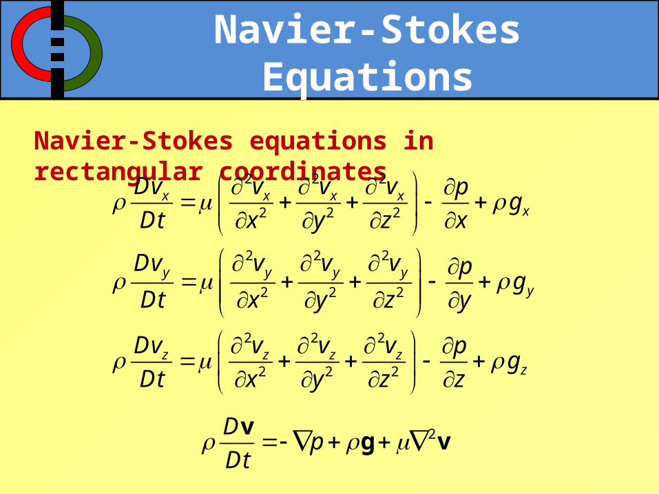
Navier-Stokes Equations
Navier-Stokes equations in rectangular coordinates2 2 2
2 2 2
2 2 2
2 2 2
2 2 2
2 2 2
x x x xx
y y y yy
z z z zz
Dv v v v pg
Dt x y z x
Dv v v v pg
Dt x y z y
Dv v v v pg
Dt x y z z
2Dp
Dt
vg v
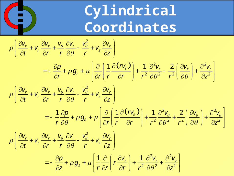
Cylindrical Coordinates
2
2 2
2 2 2 2
2
1 1 2
1
r r r rr z
r r r rr
r r r rr z
v vv v v vv v
t r r r z
rv v v vpg
r r r r r r z
v vv v v vv v
t r r r z
p
r
2 2
2 2 2 2
2
2 2
2 2 2
1 1 2
1 1
r r r rr z
z z zz
rv v v vg
r r r r r z
v vv v v vv v
t r r r z
v v vpg r
z r r r r z

Applications of Navier-Stokes Equations
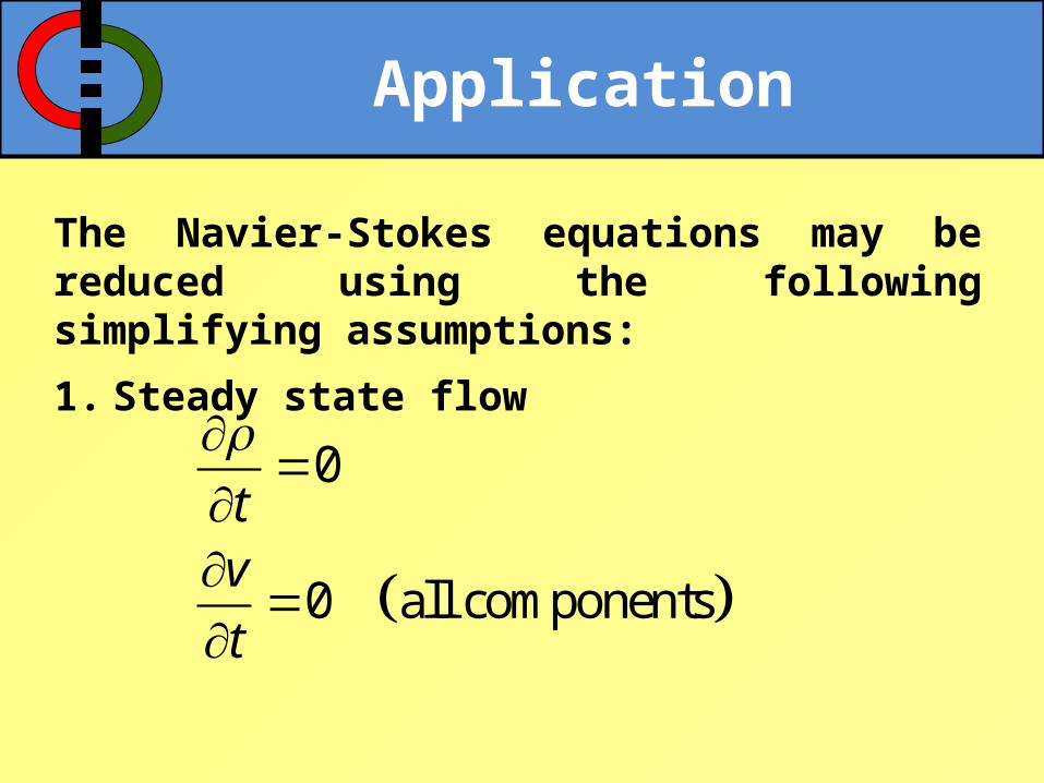
Application
The Navier-Stokes equations may be reduced using the following simplifying assumptions:
1. Steady state flow
0
0 all components
tv
t
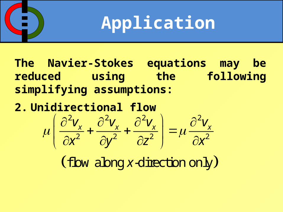
Application
The Navier-Stokes equations may be reduced using the following simplifying assumptions:
2. Unidirectional flow
2 2 2 2
2 2 2 2
flow along -direction only
x x x xv v v v
x y z x
x

Application
The Navier-Stokes equations may be reduced using the following simplifying assumptions:
2. Unidirectional flow
2 2
2 2 2 2
2
2
1 1 2
flow along -direction only
rv v v v
r r r r r z
vz
z

Application
The Navier-Stokes equations may be reduced using the following simplifying assumptions:
3. Constant fluid properties
• Isotropy (independent of position/direction)
• Independent with temperature and pressure
incompressible fluid:
0 from the equation of continuity v
Application
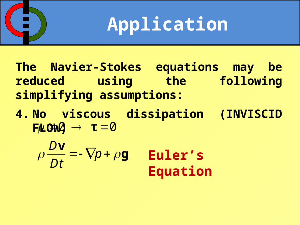
The Navier-Stokes equations may be reduced using the following simplifying assumptions:
4. No viscous dissipation (INVISCID FLOW)
0 0
Dp
Dt
τ
vg Euler’s Equation
Application
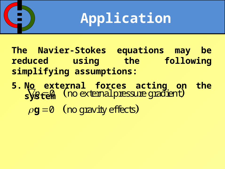
The Navier-Stokes equations may be reduced using the following simplifying assumptions:
5. No external forces acting on the system
0 no external pressure gradient
0 no gravity effects
p
g

Application
The Navier-Stokes equations may be reduced using the following simplifying assumptions:
6. Laminar flow
x x x x xx y z
Dv v v v vv v v
Dt t x y z
x xDv v
Dt t
Example
Derive the equation giving the velocity distribution at steady state for laminar flow of a constant-density fluid with constant viscosity which is flowing between two flat and parallel plates. The velocity profile desired is at a point far from the inlet or outlet of the channel. The two plates will be considered to be fixed and of infinite width, with flow driven by the pressure gradient in the x-direction.

Example
Derive the equation giving the velocity distribution at steady state for laminar, downward flow in a vertical pipe of a constant-density fluid with constant viscosity which is flowing between two flat and parallel plates.