equitable shortest job first: a preemptive scheduling

Southern Illinois University CarbondaleOpenSIUC

Articles Department of Electrical and ComputerEngineering

2014

Equitable Shortest Job First: A PreemptiveScheduling Algorithm for Soft Real-Time SystemsMario Jean ReneSouthern Illinois University Carbondale

Dimitri KagarisSouthern Illinois University Carbondale

Follow this and additional works at: http://opensiuc.lib.siu.edu/ece_articles

This Article is brought to you for free and open access by the Department of Electrical and Computer Engineering at OpenSIUC. It has been acceptedfor inclusion in Articles by an authorized administrator of OpenSIUC. For more information, please contact [email protected].

Recommended CitationRene, Mario J. and Kagaris, Dimitri. "Equitable Shortest Job First: A Preemptive Scheduling Algorithm for Soft Real-Time Systems."INTERNATIONAL JOURNAL OF ENGINEERING RESEARCH AND INNOVATION 6, No. 1 ( Jan 2014): 15-22.

http://opensiuc.lib.siu.edu?utm_source=opensiuc.lib.siu.edu%2Fece_articles%2F57&utm_medium=PDF&utm_campaign=PDFCoverPages

http://opensiuc.lib.siu.edu/ece_articles?utm_source=opensiuc.lib.siu.edu%2Fece_articles%2F57&utm_medium=PDF&utm_campaign=PDFCoverPages

http://opensiuc.lib.siu.edu/ece?utm_source=opensiuc.lib.siu.edu%2Fece_articles%2F57&utm_medium=PDF&utm_campaign=PDFCoverPages

http://opensiuc.lib.siu.edu/ece?utm_source=opensiuc.lib.siu.edu%2Fece_articles%2F57&utm_medium=PDF&utm_campaign=PDFCoverPages

http://opensiuc.lib.siu.edu/ece_articles?utm_source=opensiuc.lib.siu.edu%2Fece_articles%2F57&utm_medium=PDF&utm_campaign=PDFCoverPages

mailto:[email protected]

Abstract

The Shortest Job First (SJF) algorithm gives the optimal

average turnaround time for a set of processes, but it suffers from starvation for long processes. In this study, the authors developed an algorithm, referred to as Equitable SJF (EQ-SJF), to reduce the average turnaround time of the long pro-cesses without notably affecting the turnaround time of the short processes. Two parameters, the percentage of a pro-cess’s burst time to completion and the time spent by a pro-cess in the waiting queue, were used to provide the designer with more tradeoff alternatives in keeping the turnaround time of the long processes under control while maintaining the turnaround time of the short processes at low levels, as they are required for soft real-time tasks. Comparisons with previously proposed scheduling algorithms such as the Highest Response Ratio Next (HRRN), Railroad Strategy, Enhanced Shortest Job First (ESJF), and Alpha show that the proposed approach always offers better alternatives.

Introduction

The Shortest Job First (SJF) algorithm is a scheduling

algorithm that offers the minimum average turnaround time. This algorithm can be implemented as either preemptive or non-preemptive. In a preemptive shortest job first algorithm, the process currently running is forced to give up the pro-cessor for a new arrival process with a shorter burst time. The preemptive shortest job first algorithm is also known as the shortest remaining time (SRT) algorithm [1], [2]. In a non-preemptive shortest job first algorithm, the scheduler assigns the processor to the shortest process. Even if a short-er process becomes available, the process currently running will continue to execute until it is done. The main problem with the shortest job first algorithm is starvation [1], [2]. If there is a steady supply of short process, the long process may never get the chance to be executed by the processor.

Related Work

There is a variety of scheduling algorithms proposed in the past to solve the issue of starvation of SJF. One of the best known improvements of SJF is Highest Response Ratio

Next (HRRN) [3]. HRRN assigns a priority to each process based on its estimated run time and also on the amount of time it has spent waiting in the queue. The task priority is calculated according to the equation Priority = 1 + (WT/BT), where BT and WT are the burst time and waiting time of the process, respectively. The process with the highest priority is scheduled to run next. The longer a process is waiting in the queue, the higher the priority it accrues, thereby preventing its starvation.

In Enhanced Shortest Job First (ESJF) [4], processes are sorted in a queue in increasing order of burst time. The burst time of the first and the last processes in the queue are saved in variables ‘S’ and ‘L’, respectively. The next process is selected by comparing the values of the two variables. If ‘S’ is smaller than ‘L’ then the next shortest process is selected and its value is added to ‘S’; however, if ‘S’ is greater than ‘L’ then the largest process in the rear of the queue is select-ed to run next. The main disadvantage of ESJF is that if there are a lot of small and large processes entering the queue, the processes in the middle of the queue might not have a chance to get scheduled, causing them to starve.

Das et al. [5] proposed the Railroad Strategy in which the priority of a process is based on the equation BTi+WTi+1 < BTi+1+WTi, where BTi and WTi indicate the burst time and waiting time of process i, respectively. The burst time of process i is added to the waiting time of process i+1 and the combination, which results in the smaller value, determines the process to be scheduled next. If both sides are equal then the process with the shorter burst time is given priority. Starvation is solved because, as the waiting time of a pro-cess having a longer burst time increases, its chance of run-ning next on the processor increases.

Cherkasova [6] proposed the Alpha scheduling algorithm,

which is adjustable between First Come First Served (FCFS) and non-preemptive SJF using the equation Priority = C + alpha* BTi, where C is the amount of time the proces-sor has been servicing processes, alpha is a tuning parame-ter from 0 to ∞, and BTi is the burst time process i. If alpha is set to zero, the algorithm behaves as FCFS. If alpha is a finite number, the algorithm behaves as the non-preemptive SJF.

——————————————————————————————————————————————–———— Mario Jean Rene, Southern Illinois University at Carbondale; Dimitri Kagaris, Southern Illinois University at Carbondale

EQUITABLE SHORTEST JOB FIRST:

A PREEMPTIVE SCHEDULING ALGORITHM FOR

SOFT REAL-TIME SYSTEMS

——————————————————————————————————————————————–————

EQUITABLE SHORTEST JOB FIRST: A PREEMPTIVE SCHEDULING ALGORITHM FOR SOFT REAL-TIME SYSTEMS 15

——————————————————————————————————————————————–————

——————————————————————————————————————————————–————

16 INTERNATIONAL JOURNAL OF ENGINEERING RESEARCH AND INNOVATION | V6, N1, SPRING/SUMMER 2014

Aims/Objectives

In this current study, the authors considered that the pool of jobs to be scheduled was a mixture of computationally intensive jobs, which will be referred to here as “long’’ jobs. Low latency real-time jobs with soft deadlines [7-10] will be referred to as “short” jobs. The aim was to provide close-to-optimal average turnaround times within the soft deadline for short processes, while decreasing the average turnaround time for long processes. The SJF algorithm guar-antees the minimum average turnaround time for the short process, but this may well be below the soft deadline, in which case the longer processes could receive a better treat-ment and avoid unnecessarily long waiting times and, even-tually, starvation. The proposed methodology addresses exactly this issue: a priority is assigned to a process based (i) on the percentage of its burst time to completion con-trolled by parameter e, and (ii) on the time spent by the pro-cess in the waiting queue controlled by parameter q. Param-eter e protects a currently running process from being preempted when its remaining execution time reaches a percentage of its total burst time. Parameter q gives priority to a process when its waiting time exceeds a certain amount of its burst time. Two variants of the proposed scheduling methodology were developed and evaluated with respect to previously proposed approaches.

In the following sections, the authors describe the main algorithm, referred to as Equitable Shortest Job First (ΕQ-SJF); a variant of the algorithm, EQ-SJF with Round Robin protection (EQ-SJF-RR); experimental results comparing the proposed algorithm with previous approaches; and, fi-nally, conclusions.

EQ-SJF: Equitable Shortest Job First

The proposed Equitable Shortest Job First (EQ-SJF) algo-rithm is based on two parameters, e and q. Parameter e pro-tects the currently running process from being preempted when its execution time reaches a percentage, e%, of its total burst time. Parameter q gives priority to a process when its waiting time exceeds q times its burst time.

The pseudocode for algorithm EQ-SJF is given in Figure

1. Here, C denotes the currently running process; DNP de-notes the “do not preempt” flag; “Queue” denotes the wait-ing queue; and BT(i), WT(i), and RT(i) denote the burst time, waiting time, and remaining time of process i, respec-tively. At every cycle, algorithm EQ-SJF determines if there is a new event (i.e., an arrival or a completion). If the new event is an arrival, the algorithm examines if the queue is empty and if there is no process currently running. In that

case, the new process will become the currently running process and the DNP flag is set to 0. Otherwise, the new arrival is inserted into the waiting queue. If the new event is a process completion, the DNP flag is set to 0. After these checks for a new event, the algorithm does the following: If the Queue is not empty but there is no process currently running (i.e., C is null), the algorithm picks a job, k, with the shortest remaining time, RT(k), from the waiting queue and runs it next. Otherwise, if the queue is not empty but there is a process currently running and the DNP flag is set to 0, the algorithm does the following in order to decide whether to preempt the process or not: If RT(C) is less than or equal to e * BT(C), the current process is not going to be preempted and the DNP flag is set to 1. Otherwise, the algo-rithm examines whether there exists a process k resulting in the maximum positive value WT(k) - q * BT(k). If that is the case, the algorithm will preempt the currently running process and replace it with process k, setting the DNP flag to 1. Otherwise, the algorithm finds a process k with the minimum value RT(k). If it is less than the remaining time of the currently running process, RT(C), the currently run-ning process is preempted and is replaced by k, with the DNP flag set to 0. An illustration of the algorithm is given in Table 1 using arrival times and burst times.

Assuming that e = 0.5 and q = 0.5, the algorithm sched-ules process p1 at t=0 (see Figure 2). At t=2, p2 arrives with a burst time of 2. Process p1 has 6 cycles left to finish its execution, which is more than 50% of its burst time and because p2 has a shorter time, the scheduler preempts p1 and gives the processor to p2. Process p2 finishes execution at t=4 and p1 is scheduled next as it is the only one in the queue. After using the processor for 2 cycles, p3 arrives at t=6 with a burst time of 3. Process p1 still has 4 cycles to go, which is longer than p3, but p1 is protected from getting preempted as its remaining time is equal to or less than 50% of its burst time. Process p1 continues to run until it com-pletes execution at t=10. Next, the scheduler selects be-tween p3 with 3 cycles and p4 with 1 cycle. The scheduler selects p3, despite the fact that p4 has a shorter time, be-cause the waiting time of p3 is equal to or greater than q=0.5 times its burst time. The scheduler runs p3 for 3 cy-cles, and then p4 completes its execution at t=14.

Table 1. Process Arrival and Burst Times

PROCESS ARRIVAL TIME BURST TIME

p1 0 8

p2 2 2

p3 6 3

p4 9 1

——————————————————————————————————————————————–————

Figure 1. The EQ-SJF Scheduling Algorithm

Figure 2. Example of EQ-SJF with (e=0.5, q=0.5)

The schedules for q = 0.5 and e = 0.75, and q = 0.5 and e = 0 are given in Figures 3 and 4, respectively.

Figure 3. Example of EQ-SJF with (e=0.75 and q=0.5)

Figure 4. Example of EQ-SJF with (e=0, q=0.5)

Figures 5-7 refer to the case where the algorithm is inde-pendent of q–indicated by q =∞. At e=0, EQ-SJF behaves as the normal shortest job first with preemption and at e =1 it behaves as the normal shortest job first without preemption. The example schedules in this case for e = 0.5, e = 0.75, and e =0 are given in Figures 5-7, respectively.

Figure 5. Example of EQ-SJF with (e=0.5, q=∞)

Algorithm EQ-SJF 1. Check for new event;

2. if (event == “Arrival”){ 3. if ( (Queue, C) == ( Empty, Null) ) 4. {set C to the new arrival; set DNP = 0;} 5. else 6. add new arrival to Queue; 7. } 8. else if (event == “Completion”) 9. {set C to Null; set DNP = 0;}

10. if ((Queue, C) == ( Non-Empty, Null) ) { 11. find process k with the min value

rk =minj{RT(j)}; 12. set C to k; set DNP = 0;

13. }else if ((Queue, C) == ( Non-Empty, Non-Null)

and ( DNP == 0)) {

14. if( RT(C) ≤ e * BT(C) ) set DNP = 1; 15. else{ 16. find process k with max value

wk = maxj{WT(j)- q * BT(j)} 17. if (wk > 0){ 18. add C to Queue; 19. set C = k; set DNP = 1; 20. } else{ 21. find process k with the min value

rk =minj{RT(j)}; 22. if (rk < RT(C)){ 23. add C to Queue; 24. set C = k; set DNP = 0; 25. } 26. } 27. } 28. }

2

2

2 4

1

3

0 1 2 3 4 5 6 7 8 9 1011121314

p1

p2

p3

p4

——————————————————————————————————————————————–————


——————————————————————————————————————————————–————

——————————————————————————————————————————————–————


Figure 6. Example of EQ-SJF with (e=0.75, q=∞)

Figure 7. Example of EQ-SJF with (e=0, q=∞)

EQ-SJF with Round Robin

In the EQ-SJF algorithm, a “short” real-time process may

be denied immediate service (line 13 in Figure 1 when DNP = 0) if the currently running process has reached its e threshold (line 14 in Figure 1, whereby DNP was set to 1). Also, a “short” real-time process may be preempted by an-other process that has reached its q threshold (lines 16-19 in Figure 1). In either of these cases, the short process may have to wait a relatively long time interval with respect to its deadline in order to regain the processor. For this reason, a modification to the basic EQ-SJF algorithm is not to allow the process that has gained access to the processor, due to its e or q threshold, to hold the processor exclusively (by setting the DNP to 1). Rather, the processor can be shared in a round robin (RR) fashion among that process and a num-ber r of the processes that have the shortest remaining time. Round robin sharing is done until the first process finishes its execution. This version is referred to as EQ-SJF-RR and is described next, using the example processes from Table 1.

The case for q=0.5, e=0.5, and r=1 is shown in Figure 8. The scheduling is the same as for the example of Figure 2, until time t=6. At t=6, process p3 arrives with a burst time

of 3 cycles. Process p1 with a remaining time of 4 cycles, which is larger than p3, is protected from giving up the pro-cessor completely as its remaining time is equal to or less than 50% of its burst time. At this point, the scheduler goes to round robin between p1 and the shortest process in the queue, which is p3. Process p4 arrives at t=9 with a burst time of 1 cycle, but the scheduler continues doing round robin between p1 and p3 because r=1. Process p3 finishes its execution at t=11. The scheduler continues performing round robin with p1 and the shortest process in the queue, which is now p4. Process p1 runs for 1 more cycle and gives up the processor at t=12. Process p4 finishes at t=13 and p1, being the only process left in the queue, takes over the pro-cessor and finishes execution at t=14.

Figure 8. Example of EQ-SJF-RR with (e=0.5, q=0.5, r=1) The schedules for (e = 0.75, q = 0.5, r=1) and (e = 0, q = 0.5, r=1) are given in Figures 9 and 10, respectively.

Figure 9. Example of EQ-SJF-RR with (e=0.75, q=0.5, r=1)

Figure 10. Example of EQ-SJF-RR with (e=0, q=0.5, r=1)

2 6

2

1

3

0 1 2 3 4 5 6 7 8 9 1011 1213 14

p1

p2

p3

p4

2

2

2

3

1

4

0 1 2 3 4 5 6 7 8 9 1011 1213 14

p1

p2

p3

p4

2

2

2

1

1

1

1

1

1

1

1

0 1 2 3 4 5 6 7 8 9 10 11 12 13 14

p1

p2

p3

p4

2

1

1

1

1

1

1

1

1

1

1

1

1

1 2 3 4 5 6 7 8 9 10 11 12 13 14

p1

p2

p3

p4

2

2

2

2

1

1

1

1

1 1

0 1 2 3 4 5 6 7 8 9 10 11 12 13 14

p1

p2

p3

p4

——————————————————————————————————————————————–————

Experimental Evaluation

The proposed scheduling algorithms EQ-SJF and EQ-SJF-RR were implemented in C and their performance was evaluated against that of SJF, HRRN [3], ESJF [4], Railroad Strategy [5], and Alpha [6]. Two arrival traffic patterns were generated: random and peak random. For the random arrival pattern, the arrival times were randomly generated for all of the processes. For the peak random pattern (i.e., for every randomly selected time at which a long process arrives) a number (e.g., 10 or 20) of short processes were generated at the same arrival time. The burst times of the long processes were randomly generated from 40 to 50 and 80 to 100 time units. The burst times of the short processes were randomly generated from 1 to 10 time units. In all cas-es, the total average turnaround times for all processes (TATT), along with the average turnaround time for long processes (LATT) and average turnaround time for short processes (SATT), were computed.

Rationale and Analysis

Tables 2-9 show the TATT, LATT, and SATT for the different scheduling algorithms. It should be noted that the SJF offers the best TATT but not the best LATT. The ra-tionale in comparing these algorithms was to see which one offered the next best SATT (after the one that SJF offers) in order to reduce the LATT. The amount of the LATT reduc-tion is of secondary importance in these comparisons since the priority was not to significantly increase the SATT of the soft real-time processes and, thus, avoid violating their ultimate deadlines.

The first column in each of the tables shows the algo-rithms; the second column shows the TATT; the third col-umn shows the LATT; and the last column shows the SATT. Row 3 shows the results for the Preemptive Shortest Job First algorithm (SJF), and rows 4-7 show the results for Railroad, HRRN, ESJF, and the Alpha scheduling algo-rithms. The remaining rows contain the results for different configurations of the proposed algorithm.

Tables 2-5 show the results for the random arrival traffic pattern. In all of these tables, the number of short processes was fixed to 500 and their burst times were randomly select-ed from 1 to 10 time units. The number of the long process-es was fixed at 50. The burst times of the long jobs were randomly selected from 40 to 50 time units in Tables 2 and 3, and from 80 to 100 time units in Tables 4 and 5. The arri-val range for a processes was from 0 to A=2500 (“sparse” arrivals) and A=1250 (“dense” arrivals) time units for Ta-bles 2 and 3, respectively; and from 0 to A=5000 (“sparse” arrivals) and A=2500 (“dense” arrivals) time units for Ta-

bles 4 and 5, respectively. Tables 6-9 show the results for the peak random arrival traffic, under the exact same setups as those corresponding to Tables 2-5. The values of parame-ter e used for the configurations of the proposed algorithms were e = 0, 0.25, 0.5, 0.75, and 1.0. An upper bound on the values that parameter q can take was determined by the ratio of the LATT offered by SJF to the average burst time of the long jobs. For example, in Table 2, that ratio is 2487/45 = 55.27. Finally, the value of parameter r was kept to less than or equal to 3.

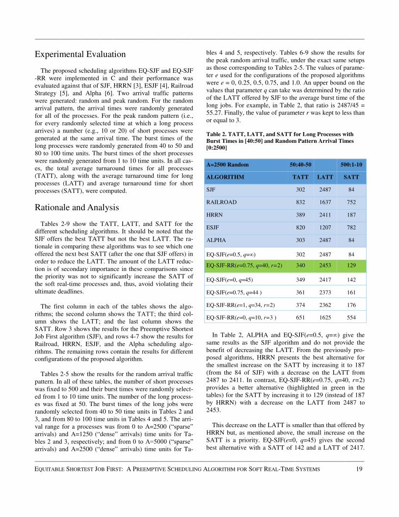
Table 2. TATT, LATT, and SATT for Long Processes with

Burst Times in [40:50] and Random Pattern Arrival Times

[0:2500]

In Table 2, ALPHA and EQ-SJF(e=0.5, q=∞) give the same results as the SJF algorithm and do not provide the benefit of decreasing the LATT. From the previously pro-posed algorithms, HRRN presents the best alternative for the smallest increase on the SATT by increasing it to 187 (from the 84 of SJF) with a decrease on the LATT from 2487 to 2411. In contrast, EQ-SJF-RR(e=0.75, q=40, r=2) provides a better alternative (highlighted in green in the tables) for the SATT by increasing it to 129 (instead of 187 by HRRN) with a decrease on the LATT from 2487 to 2453.

This decrease on the LATT is smaller than that offered by

HRRN but, as mentioned above, the small increase on the SATT is a priority. EQ-SJF(e=0, q=45) gives the second best alternative with a SATT of 142 and a LATT of 2417.

A=2500 Random 50:40-50 500:1-10

ALGORITHM TATT LATT SATT

SJF 302 2487 84

RAILROAD 832 1637 752

HRRN 389 2411 187

ESJF 820 1207 782

ALPHA 303 2487 84

EQ-SJF(e=0.5, q=∞) 302 2487 84

EQ-SJF-RR(e=0.75, q=40, r=2) 340 2453 129

EQ-SJF(e=0, q=45) 349 2417 142

EQ-SJF(e=0.75, q=44 ) 361 2373 161

EQ-SJF-RR(e=1, q=34, r=2) 374 2362 176

EQ-SJF-RR(e=0, q=10, r=3 ) 651 1625 554

——————————————————————————————————————————————–————


——————————————————————————————————————————————–————

——————————————————————————————————————————————–————


This LATT is very close to that offered by HRRN but the increase of the SATT is significantly smaller (142 versus 187 of the HRRN). EQ-SJF(e=0.75, q=44) not only offers a better option than HRRN with a smaller increase on the SATT from 187 to 161, but also achieves a larger decrease on the LATT from 2411 to 2373. EQ-SJF-RR(e=1, q=34, r=2) provides the same benefits offering a SATT of 176 and a LATT of 2362. If one is willing to allow a still higher in-crease on the SATT, RAILROAD offers the best alternative among the previously proposed algorithms with a SATT of 752 and a LATT of 1637. However, from the algorithms proposed in this current study, EQ-SJF-RR(e=0, q=10,r=3) provides a better alternative by offering both a smaller SATT of 554 and a larger decrease on the LATT from 1637 to 1625.



[0:1250]

The designer/system manager will ultimately decide what increase on the SATT is acceptable, based on the deadlines of the real-time processes which are treated here as the “short” processes. The benefit of the proposed approach is that it provides the designer with many more alternatives for increasing the SATT. In the aforementioned approaches, the designer would have no alternative except to choose HRRN, which offers a SATT of 187, but this may be too much giv-en that the SATT that the SJF offers for the real time pro-cess is 84. In contrast, the proposed approach provides a series of alternatives for increasing the SATT to 129, 142, 161, and 176. Assuming, for instance, that twice the SATT that SJF offers is still acceptable for the deadlines of the real

-time processes, the first three of these alternatives would be acceptable but none of the previous approaches would be.



[0:5000]



[0:2500]

A=1250 Random 50:40-50 500:1-10


SJF 660 2975 429

RAILROAD 1145 2404 1019

HRRN 743 2995 518

ESJF 1249 1690 1205

ALPHA 661 2975 429

EQ-SJF(e=0.5,q=∞) 661 2975 429

EQ-SJF(e=0.5, q=52) 692 2928 469

EQ-SJF(e=0.25, q=50) 711 2876 495

EQ-SJF-RR(e=1, q=40, r=1) 719 2860 504

EQ-SJF(e=0, q=40) 884 2350 738

EQ-SJF(e=0, q=26) 1149 1681 1096

A=5000 Random 50:80-100 500:1-10


SJF 193 2040 9

RAILROAD 930 1505 872

HRRN 300 1990 130

ESJF 319 2053 146

ALPHA 223 1994 46

EQ-SJF-RR(e=0.5, q=∞, r=1) 196 2034 12

EQ-SJF(e=0.5, q=∞) 198 2024 15

EQ-SJF-RR(e=1, q=6, r=1) 206 2026 24

EQ-SJF(e=0.5, q=38) 218 2017 38

EQ-SJF(e=1, q=40) 239 1987 64

EQ-SJF(e=0, q=17) 764 1500 691

A=2500 Random 50:80-100 500:1-10


SJF 433 3737 103

RAILROAD 1333 2990 1168

HRRN 517 3730 195

ESJF 1134 3121 936

ALPHA 434 3727 103

EQ-SJF(e=0.5,q=∞) 433 3737 103

EQ-SJF-RR(e=0.75, q=22, r=2) 504 3727 182

EQ-SJF(e=0.25, q=28) 507 3713 187

EQ-SJF(e=0.5, q=22) 1064 3117 860

EQ-SJF-RR(e=0.75, q=1, r=1) 1146 2954 1168

——————————————————————————————————————————————–————


Burst Times in [40:50] and Peak Random Pattern Arrival

Times [0:2500]



Times [0:1250]

Similar observations hold for the other tables. For in-stance, in Table 8, SJF offers the best SATT with a value of 43. The next best alternative among the previously proposed algorithms for an increase on the SATT in order to reduce the LATT is offered by ALPHA with a SATT of 77 and a decrease on the LATT from 1594 to 1550. However, the proposed approach provides a series of better alternatives—EQ-SJF-RR(e=0.5 r=1), EQ-SJF(e=0.5, q=∞), EQ-SJF-RR(e=0.75,q=59, r=1), EQ-SJF(e=0.75,q=56)—that increase the SATT to 46, 47, 59, and 63, respectively, and reduce the LATT to 1584, 1582, 1566, and 1559, respectively.



Times [0:5000]

Overall, the proposed approach provides the designer with a lot of flexibility on what type of algorithm to select depending on the SATT for the soft real-time jobs. If the designer wants the short processes to execute faster, the designer can increase q; if the designer wants the long pro-cesses to have a lower LATT, the designer can decrease q, thus giving the long processes higher priority and prevent-ing starvation when they reach a certain amount of waiting time. Also, by using small values of e, the designer can ap-proximate the behavior of SJF with preemption. Or, by us-ing larger values of e (close to 1), the designer can approxi-mate the behavior of SJF without preemption. The specific values of e and q and their effect on SATT are found by simulation.

A=2500 Peak Random 50:40-50 500:1-10


SJF 413 2725 181

RAILROAD 954 1901 859

HRRN 495 2695 275

ESJF 989 1327 955

ALPHA 413 2725 181

EQ-SJF(e=0.25, q=∞) 413 2725 181

EQ-SJF(e=0.25, q=53) 447 2678 224

EQ-SJF-RR(e=1, q=44, r=2) 457 2645 239

EQ-SJF-RR(e=0, q=44, r=1) 466 2618 251

EQ-SJF(e=0.25, q=51) 475 2582 264

EQ-SJF(e=1, q=36) 752 1858 641

EQ-SJF-RR(e=0,q=4, r=1) 977 1294 946

A=1250 Peak Random 50:40-50 500:1-10


SJF 701 3191 452

RAILROAD 1084 2624 929

HRRN 797 3155 561

ESJF 1367 1708 1331

ALPHA 701 3191 452

EQ-SJF(e=0.5, q=∞) 701 3191 452

EQ-SJF(e=0, q=51, r=2) 737 3142 497

EQ-SJF(e=0.25, q=58) 745 3115 508

EQ-SJF-RR(e=0.5, q=47, r=2) 757 3089 523

EQ-SJF(e=0.75, q=56) 773 3020 548

EQ-SJF(e=0.75, q=46) 936 2539 776

EQ-SJF(e=0.5, q=28) 1310 1689 1272

A=5000 Peak Random 50:80-100 500:1-10


SJF 184 1594 43

RAILROAD 616 1278 550

HRRN 261 1569 130

ESJF 408 1444 305

ALPHA 211 1550 77

EQ-SJF(e=0.5,q=∞, r=1) 186 1584 46

EQ-SJF(e=0.5, q=∞) 187 1582 47

EQ-SJF-RR(e=0.75, q=59, r=1) 196 1566 59

EQ-SJF(e=0.75, q=56) 199 1559 63

EQ-SJF(e=0.25, q=17) 387 1419 283

EQ-SJF(e=75, q=14) 575 1237 508

——————————————————————————————————————————————–————


——————————————————————————————————————————————–————

——————————————————————————————————————————————–————




Times [0:2500]

Conclusion

The proposed approach presents the designer with a varie-ty of choices in selecting a scheduling algorithm that pro-vides close-to-optimal average turnaround times of short processes, considered here to be soft real-time processes, while decreasing the turnaround time of the long processes that run in the same job mix with the short processes. The proposed algorithms address the drawback related to the long-process starvation in SJF by providing protection to a process through prioritization. The priority to a process is assigned based on a percentage of its burst time to comple-tion (controlled by parameter e) or the time spent by the process in the waiting queue (controlled by parameter q). Experimental results showed that the proposed approach always offered the next best alternative (indicated in green in the Tables) to SJF in terms of offering the smallest in-crease in SATT while reducing the LATT. The proposed approach can be incorporated into more complicated sched-uling algorithms for ensuring quality of service in soft real-time systems.

References [1] Silberschatz, A., Galvin P. B., & Gagne G. (2004).

Operating System Concepts, (7th ed.), Wiley. [2] Stallings, S. (2004). Operating Systems Internals and

Design Principles, (5th ed.). Prentice Hall.

[3] Tanenbaum, A. S. (2007). Modern Operating Sys-

tems, (3rd ed.), Prentice Hall. [4] Shahzad, B., & Afzal, M. T. (2006). Optimized Solu-

tion to Shortest Job First by Eliminating the Starva-tion. Proceedings of Jordanian International Electri-

cal and Electronics Engineering Conference. [5] Jain, S., Mishra, V., Kumar, R., & Jaiswal, U. C.

(2011). Railroad Strategy for SJF Starvation Prob-lem. Proceedings of Computer Networks and Infor-

mation Technologies, 403–408. [6] Cherkasova, L. (1998). Scheduling Strategy to Im-

prove Response Time for Web Applications. Pro-

ceedings of High Performance Computing and Net-

working, 305-314. [7] Ahmed, S., & Ferri, B. (2013). Prediction-Based

Asynchronous CPU-Budget Allocation for Soft Real-Time Applications. IEEE Transactions on Comput-

ers. [8] Khalib, Z. I. A., Ahmad, B. R., & Ong, O. B. L.

(2012). High Performance Non-Preemptive Dynamic Scheduling Algorithm for Soft Real Time System. IEEE Symposium on Computer Applications and

Industrial Electronics, 54-59. [9] Raeisi, R., & Singh, S. (2010). An Innovative Imple-

mentation Technique of a Real-Time Soft-Core Pro-cessor. International Journal of Modern Engineering,

64-68. [10] Balarin, F., Lavagno, L., Murthy, P., & Vincentelli

A. S. (1998). Scheduling for Embedded Real-Time Systems. IEEE Design & Test of Computers, 71–82.

Biographies

MARIO JEAN RENE is a graduate student for the MS degree in electrical and computer engineering at Southern Illinois University, Carbondale. He earned his BS degree in Computer Engineering in 2007 from the ECE Department, Southern Illinois University, Carbondale.

DIMITRI KAGARIS is a professor in the Electrical and Computer Engineering Department, Southern Illinois Uni-versity, Carbondale. His research interests are in digital de-sign automation, embedded systems, sensor networks, and data mining. Email: [email protected]

A=2500 Peak Random 50:80-100 500:1-10


SJF 501 3613 189

RAILROAD 1250 3081 1067

HRRN 607 3615 306

ESJF 1136 3084 941

ALPHA 536 3562 234

EQ-SJF(e=0.75, q=∞) 501 3613 189

EQ-SJF-RR(e=1, q=68, r=3) 532 3567 229

EQ-SJF-RR(e=1, q=77, r=1) 533 3566 230

EQ-SJF(e=0.5, q=20) 1108 2915 920

equitable shortest job first: a preemptive scheduling

Documents