equities, credits and volatilities: a multivariate analysis - mediatum

Equities, Credits and Volatilities:

A Multivariate Analysis of the European Market

During the Sub-prime Crisis

Irene Schreiber, Gernot Muller, Claudia Kluppelberg, Niklas WagnerTechnische Universitat Munchen und Universitat Passau

Version: 2009-10-07

Abstract

Motivated by recent developments in light of the sub-prime and subsequent financial crisis wefit two different vector autoregressive generalized conditional heteroscedastic (VAR-GARCH)models to three financial indices with the aim of understanding the development of dependencystructures between credit spreads and other macroeconomic variables. Our analysis includesdaily quotes from June 2004 to April 2009 of the iTraxx Europe index, the Dow Jones EuroStoxx 50 index, and the Dow Jones VStoxx index. We propose a robust, time-varying modelingapproach concerning the conditional mean, and a BEKK versus DCC-GARCH approach con-cerning the conditional covariance. Furthermore we allow for a parsimonious model specificationby setting insignificant coefficients to zero. Our empirical results indicate that the autoregressivecoefficients vary strongly with time and even change their signs. Well-known interrelations, suchas the negative correlation between CDS’ and stocks are lost through the financial crisis. Theconditional covariance estimates in the BEKK and DCC model are fairly similar, given the dif-ference in the number of model parameters. We found evidence of strongly varying conditionalvariances and correlations, with dependencies increasing after the outbreak of the financial crisis.This knowledge may help to improve decision tools in the financial industry, especially in areassuch as asset pricing, portfolio selection, and risk management.

Keywords: credit risk, credit default swaps, iTraxx index, vector autoregression, multivariateGARCH, VAR-GARCH, BEKK, DCC.

1 INTRODUCTION 2

1 Introduction

Recent developments in light of the U.S. sub-prime and the subsequent financial crisis in 2008have shown, that credit derivatives may be more closely related to other asset classes thanpreviously suspected. This has made the understanding of dependency structures a key issue inbusiness-oriented finance and subject to extensive research. In particular, many authors havestudied the relationship between financial derivatives and other asset classes, such as equities andbonds, in order to understand the contamination of the global capital markets by the precedingUS sub-prime crisis. For this purpose, credit default swaps (CDS), which are understood to be atthe core of the sub-prime crisis, have been extensively investigated. Examples of empirical studiesof CDS’ and their relationship with other macroeconomic variables include Houweling and Vorst(2005), Bystrom (2005, 2006), Alexander and Kaeck (2006), Sougne et al. (2008), Ericsson et al.(2009) and Norden and Weber (2009). However, these authors concentrate on modeling theconditional mean, e.g. by fitting regression type models, whereas our modeling approach goesone step further by including the conditional covariance structure in the model. More precicely,this paper presents an investigation into the dependency structure of equities, credit spreads andvolatilities in the European market by means of the three time series iTraxx Europe, Euro Stoxx50, and VStoxx index. We fit a VAR-BEKK and a VAR-DCC model to our three dimensionaltime series of daily quotes from June 2004 to April 2009. Main innovations of our approach are therobust time-varying multivariate modeling approach as well as the combination of two differentmodels, namely the vector autoregressive (VAR) and the multivariate GARCH (MGARCH)model.

It is worth mentioning that the starting point of our analysis was the data set of the iTraxxEurope family itself, and the attempt to model dependencies between different classes of ag-gregated credit spreads, e.g. between the iTraxx Senior Financials and Sub Financials. Thisquestion could be addressed adequately by a co-integration type modeling approach. However,the sub-indices of the iTraxx Family are far less liquid than the benchmark index iTraxx Eu-rope. Therefore, due to long passages of missing values in the time series as a consequence ofthe financial crisis and the subsequent drying-out of the CDS market, the data set is unsuitablefor an empirical study with this purpose.

In our paper we focus on modeling dependencies between aggregated credit spreads by meansof the iTraxx Europe index and other asset classes. In a first, preceding study, in addition tostocks and stock market volatility, we also included long and short term interest rates by meansof the LIBOR three months interest rate and a European government bond index by Bloombergin our analysis, i.e. in a multivariate VAR-GARCH model with five time series. However, theinterest rates were found to deliver no additional explanatory information considering the condi-tional mean structure. Moreover, with these five time series, the conditional covariance structurewas not able to be captured by the different MGARCH models.

The first part of our modeling framework is based on VAR models, which have proven veryuseful to capture the evolution and the interdependencies of multiple time series. Introduced by

1 INTRODUCTION 3

Sims (1972, 1980), they have been used for a variety of purposes such as data description andforecasting, as well as structural inference and policy analysis. The theoretical background onVAR models has been extensively explored and discussed in the literature, see e.g. Hannan(1970), Brockwell and Davis (1991), Lutkepohl (1991, 2005) and Hamilton (1994). For ourpurpose we extend the classical VAR modeling approach by admitting time-varying coefficientsand by following a robust iteratively re-weighted least squares approach (see Huber, 1981),thereby reducing the influence of outliers and enhancing the model adequacy.

When investigating financial time series, it is a well known fact that models based on thehomoscedasticity assumption are not sufficient to grasp stylized features such as volatility clus-tering and time-varying correlations. The second part of our modeling approach therefore isbased MGARCH models, which in this context provide an ideal setting for investigating de-pendency structures of different financial time series. The widespread use of MGARCH modelsas an extension of the univariate ARCH and GARCH models by Engle (1982) and Bollerslev(1986) dates back to the well known VEC or so called general MGARCH model, first proposedby Bollerslev et al. (1988). From this starting point the theoretical development branches out,and as a result a variety of different MGARCH models evolved over the past two decades (seeLi et al., 2002 and Bauwens et al., 2006, for recent reviews). As opposed to the univariate case,a coherent theory valid for all MGARCH models has yet to be developed. To cover all modelstherefore goes beyond the scope of this paper. In contrast, we deliberately focus on the two mostwell known and frequently used models in practice, namely the BEKK and the DCC model,which will be discussed here.

Engle and Kroner (1995) introduce the famous BEKK model as a special case of the VECmodel by Bollerslev et al. (1988), which entailed the development of various subclasses and sim-ilar modeling approaches. The main advantage of this model is, that the BEKK parametrizationautomatically guarantees the positive definiteness of Ht. Besides that, the number of parametersin comparison with the general VEC model is remarkably reduced.

The key idea behind another class of MGARCH models is the nonlinear combination of uni-variate GARCH models, thus enabling separate modeling of variances and correlations. Probablythe most popular model in practice is the well known dynamic conditional correlation (DCC)model by Engle and Sheppard (2001), which was introduced as a generalization of the constantconditional correlation (CCC) model by Bollerslev (1990). One reason why the DCC modelis very popular with practitioners is its parsimony, as the model enables keeping the numberof parameters relatively low (in comparison with both the VEC and BEKK model). Anotheradvantage of this model lies in its flexibility, i.e. the univariate GARCH equations for the con-ditional variances may be specified by any kind of univariate GARCH parametrization, therebyincluding special model classes such as nonlinear or exponential GARCH models (see Engle andSheppard, 2001, 2002).

The remainder of this paper is organized as follows: in Section 2 we briefly introduce thenecessary modeling framework. Section 3 is dedicated to a multivariate empirical study of theiTraxx, Euro Stoxx 50 and VStoxx. Section 4 then concludes this paper with a brief summary

2 MODEL SPECIFICATION AND ESTIMATION 4

of the main steps and most important findings on the topic.

2 Model Specification and Estimation

2.1 Model

In this section we briefly introduce the necessary theory which we will apply to our data inSection 3. All stochastic objects in this paper are defined on the probability space (Ω,F, P ).Consider a vector stochastic process (yt)t∈Z, i.e. yt : Ω → RN . As usual, we condition on thesigma field, denoted by Ft−1, generated by the past information until time t− 1. Note that wewill follow the convention of using lowercase letters to denote either a random variable or itsrealization as a time series. In this paper we will consider the following vector autoregressivegeneralized conditional heteroscedastic (VAR-GARCH) model:

yt = c+ Φ1yt−1 + · · ·+ Φpyt−p + εt, (1)

εt = H1/2t (θ)zt, zt ∼WN(0, IN ) i.i.d., (2)

where c ∈ RN denotes a vector of constants, Φ1, . . . ,Φp ∈ RN×N are matrices of autoregressivecoefficients and θ ∈ Θ contains all GARCH parameters. Furthermore, (zt)t∈Z is a multivariatewhite noise process, IN ∈ RN×N as usual is the identity matrix and H

1/2t (θ) ∈ RN×N is a

positive definite matrix, such that Ht is the conditional covariance matrix of yt, e.g. H1/2t may

be obtained by the Cholesky factorization of Ht.The conditional mean part of the model in (1) is given by a VAR model of order p, while

the conditional covariance matrix Ht in (2) is specified by an MGARCH model. As mentionedabove, in this work we focus on the two most prominent models, the BEKK and the DCC model,which will be briefly discussed here.

Assume (yt), (εt) and (zt) to be vector stochastic processes as given by (1) and (2). TheBEKK(p,q)1 model by Engle and Kroner (1995) for the conditional covariance matrix Ht ∈RN×N is defined as

Ht = C ′C +q∑

i=1

A′iεt−iε′t−iAi +

p∑j=1

B′jHt−jBj , (3)

where Ai, Bj ,∈ RN×N are parameter matrices and C ∈ RN×N is an upper triangular matrix.As mentioned above the main advantage of this model is, that the BEKK parametrizationautomatically guarantees the positive definiteness ofHt. The number of parameters in the BEKKmodel is N(N + 1)/2 + N2(p + q), i.e. O(N2). In order to reduce the number of parameters,different simplifications of the model evolved, e. g. the diagonal BEKK model where Ai andBj in (3) are diagonal matrices or the scalar BEKK model where Ai and Bj are each replaced

1The acronym BEKK stands for Baba, Engle, Kraft & Kroner who wrote an earlier version of the paper byEngle and Kroner (1995) (see Engle, Kroner, Baba, and Kraft, 1993).


by a scalar times a matrix of ones. To ensure the uniqueness of the parametrization, certainrestrictions have to be imposed on the coefficient matrices. For instance, in the special caseof the BEKK(1,1) model with Ht = C ′C + A′εt−1ε

′t−1A + B′Ht−1B and parameter matrices

A = (Aij)Ni,j=1, B = (Bij)N

i,j=1 Engle and Kroner (1995) show, that uniqueness is achieved byrequesting all diagonal elements of C to be positive, as well as A11, B11 > 0. These conditionsfor the coefficient matrices can be extended to the general case when p, q > 1. Engle and Kroner(1995) also show, that the BEKK model as defined in (1), (2) and (3) is stationary if and onlyif all eigenvalues of the matrix

∑qi=1A

′i ⊗Ai +

∑pj=1B

′j ⊗Bj are less than one in modulus.

The second model for the conditional covariance matrix in (2) which we will consider in thispaper is the dynamic conditional correlation (DCC) model by Engle (2002). The key idea of thismodel is to specify the conditional covariance matrix Ht in two steps. First, a univariate GARCHmodel is chosen for each individual conditional variance Hii,t, i = 1, . . . , N . Second, based on theindividual conditional variances the conditional correlation matrix is specified, thereby imposingits positive definiteness. The DCC(p,q) model for the conditional covariance matrix Ht ∈ RN×N

is defined as

Ht = DtRtDt, with Dt = diag(H1/211,t, . . . ,H

1/2NN,t). (4)

The elements of Dt are defined as univariate GARCH models, i.e. ∀ i = 1, . . . , N we define

Hii,t = ωi +qi∑

q=1

αiqε2i,t−q +

pi∑p=1

βipHii,t−p, (5)

with the usual restrictions for non-negativity and stationarity being imposed ∀ i = 1, . . . , N :

(i) ωi > 0,

(ii) ∀ p = 1, . . . , pi, ∀ q = 1, . . . , qi : αiq, βip are such that Hii,t will be positive with proba-bility one,

(iii)∑qi

q=1 αiq +∑pi

p=1 βip < 1.

The dynamic correlation structure is given by

Qt = (1−M∑

m=1

am −N∑

n=1

bn)Q+M∑

m=1

am(νt−mν′t−m) +

N∑n=1

bnQt−n, (6)

Rt = diag(Q1/211,t, . . . , Q

1/2NN,t)

−1Qt diag(Q1/211,t, . . . , Q

1/2NN,t)

−1, (7)

with νt := D−1t εt, and Q being the unconditional covariance matrix of νt : νt ∼ N (0, Q). We

refer to Engle and Sheppard (2001, Proposition 2) for sufficient conditions regarding the positivedefiniteness of Ht.


2.2 Estimation Method

Regarding the estimation of the model parameters in (1), (2) and (3), (4)–(5), respectively, wefollow a two step approach, where in the first step the parameters of the VAR model, and in thesecond step the GARCH parameters are estimated.

Concerning the VAR model coefficients we pursue the robust iteratively re-weighted leastsquares (RLS) approach of Huber (1981). Assume that the sample size is T and that we aregiven p pre-sample values y−p+1, . . . , y0. We define:

Y := (y1, . . . , yT ) ∈ RN×T ,

Π := (c,Φ1, . . . ,Φp) ∈ RN×(Np+1), π := vec(Π) ∈ RN(Np+1),

xt := (1, y′t−1, . . . , y′t−p)

′ ∈ RNp+1, X := (x1, . . . , xT ) ∈ R(Np+1)×T ,

E := (ε1, . . . , εT ) ∈ RN×T ,

where vec(·) is the column stacking operator that stacks the columns of a m × n matrix as avector of dimension mn. Using this notation we may then rewrite (1) as a linear model

Y = ΠX + E, or equivalently vec(Y ) = (X ′ ⊗ IN )π + vec(E), (8)

where ⊗ denotes the Kronecker product or direct product of two matrices. Note that as opposedto classical linear modeling, the matrix of covariables contains lagged dependent variables.The unknown parameters of the VAR model contained in π in (8) are then estimated by theRLS approach of Huber (1981), who introduces the class of M-estimates, in order to reducethe influence of outliers and achieve distributional robustness. We investigate the problem∑NT

i=1 ρ(xi ; π) = min!, or equivalently∑NT

i=1 ψ(xi ; π) =∑NT

i=1wixi = 0, where xi is the i-thresidual of the NT -dimensional linear model in (8), ρ(x ; π) is a weighting function, ψ(x) :=(∂/∂θ)ρ(x ; π) and wi := ψ(xi ; π)/xi. The weighting function ρ(x ; π) is assumed to be twicecontinuously differentiable in x almost everywhere, with nonnegative second derivative whereverdefined. Huber (1981) proposes

ρ(x) =

x2/2 : |x| ≤ c,

c|x| − c2/2 : |x| > c,(9)

which implies weights wi = 1 if |xi| ≤ c and wi = c/xi if |xi| > c. In the context of VAR modelsstrong consistency of the RLS estimator is e.g. shown by Campbell (1982), while asymptoticnormality is derived by Li and Hui (1989).

We now briefly discuss estimation procedures for the BEKK and DCC-GARCH model. In thecase of the BEKK model given by (2) and (3) we perform maximum likelihood (ML) estimation.


Assume we have a given sample size of t = 1, . . . , T . The log likelihood function is then given by

L(θ) = −12

T∑t=1

(N ln(2π) + ln |Ht(θ)|+ ε′tHt(θ)−1εt), (10)

where θ := vec(C,A1, . . . , Aq, B1, . . . , Bp) ∈ Θ ⊂ RN(N+1)/2+N2(p+q) contains all unknownGARCH parameters. The likelihood function is maximized with respect to θ by using numericalmethods. A closed form solution does not necessarily exist, due to the nonlinearity of the like-lihood function. For asymptotic properties of the ML estimator, see e.g. Comte and Lieberman(2003), who derive strong consistency and asymptotic normality.

According to Engle and Sheppard (2001), the DCC model as defined in (4)–(7) was designedto allow for a two-stage estimation procedure. They suggest decomposing the parameter vector θinto two disjoint parts, one for the individual conditional volatilities and one for the conditionalcorrelations. Then in the first stage univariate GARCH models for each component of εt =(ε1t, . . . , εNt) are estimated. In the second stage, using transformed residuals resulting from thefirst stage, an estimator for the conditional correlations is derived. As Ht = DtRtDt in the DCCmodel according to (4), the likelihood function in (10) may be rewritten in the following way:

L(θ) = −12

T∑t=1

(N ln(2π) + ln |DtRtDt|+ ε′tD−1t R−1

t D−1t εt)

= −12

T∑t=1

(N ln(2π) + 2 ln |Dt|+ ε′tD−1t D−1

t εt − ν ′tνt + ln |Rt|+ ν ′tR−1t νt). (11)

Let θ = (θ1, θ2) denote the parameters for the conditional volatilities and conditional correla-tions, as given in (4)–(5) and (6)–(7), respectively. The likelihood in (11) is decomposed intotwo disjoint parts:

L(θ) = L(θ1, θ2) = LV (θ1) + LC(θ2),

with a volatility part LV (θ1) := −12

∑Tt=1(N ln(2π) + 2 ln |Dt|+ ε′tD

−1t D−1

t εt) and a correlationpart LC(θ2) := −1

2

∑Tt=1(−ν ′tνt + ln |Rt|+ ν ′tR

−1t νt). The volatility part then corresponds to the

sum of the likelihood functions of N univariate GARCH models

LV (θ1) := −12

T∑t=1

N∑i=1

(ln(2π) + ln(Hii,t) +

ε2itHii,t

).

Now first solve θ1 = arg maxLV (θ1), and then subsequently θ2 = arg maxLC(θ1, θ2). Note thatEngle and Sheppard (2001) argue, that consistency and asymptotic normality of θ1 and θ2 holddue to results given by Newey and McFadden (1994) concerning consistency of an estimator in atwo-step general method of moments problem, usually resulting in a loss of efficiency. However,this argumentation is recently being questioned by e.g. Caporin and McAleer (2008, 2009), who

3 EMPIRICAL ANALYSIS 8

conclude that the properties of the DCC estimates as claimed by Engle and Sheppard (2001)cannot be derived by their course of argumentation.

3 Empirical Analysis

3.1 Data Set

Our data set consists of three time series, the Dow Jones Euro Stoxx 50 index, the Dow JonesVStoxx index, a volatility index based on options on the Euro Stoxx 50 and the CDS index iTraxxEurope. In our analysis we focus on the iTraxx Europe benchmark index with a maturity of fiveyears, as this is the most liquid index within the iTraxx Europe index family. As the membershipof the iTraxx is adjusted every six months by issuing a new index series, we construct a timeseries that contains the most recent series at any point in time. In this way we ensure thatour analysis is always built on the most liquid names. The data period starts on June 23, 2004and ends on April 30, 2009, i.e. the data set covers 1230 daily quotes for each of the timeseries. Basic characteristics of the data are summarized in Table 1. The data was transformed to

Index

01/05 01/06 01/07 01/08 01/09

5010

015

020

0

itrax

x (b

ps)

Index

01/05 01/06 01/07 01/08 01/09

−20

020

log.

diff

. itr

axx

Index

01/05 01/06 01/07 01/08 01/09

2000

3000

4000

euro

stox

x

Index

01/05 01/06 01/07 01/08 01/09

−20

020

log.

diff

. eur

osto

xx

01/05 01/06 01/07 01/08 01/09

2040

6080

vsto

xx (

%)

01/05 01/06 01/07 01/08 01/09

−20

020

log.

diff

. vst

oxx

Figure 1: Daily quotes of the iTraxx Europe, the Euro Stoxx 50 and the VStoxx index between2004-06-23 and 2009-04-30.


2004-06-23 to 2009-04-30 2004-06-23 to 2007-08-15 2007-08-16 to 2009-04-30itraxx eurost. vstoxx itraxx eurost. vstoxx itraxx eurost. vstoxx

min. 20.09 1809.98 11.60 20.09 2580.04 11.60 29.10 1809.98 17.241st qu. 31.00 2980.13 14.85 27.78 3055.85 14.03 68.28 2451.58 22.56median 37.12 3524.58 17.72 35.20 3544.58 15.67 101.38 3429.58 27.32mean 59.72 3463.51 22.13 33.38 3537.33 16.15 108.71 3326.18 33.263rd qu. 74.37 3987.13 24.00 37.19 3988.04 17.58 154.42 3881.09 42.05max. 215.92 4557.57 87.51 68.20 4557.57 30.74 215.92 4489.79 87.51std. 46.43 654.60 11.85 7.41 540.75 2.96 48.71 808.63 13.97skewn. 1.57 -0.31 2.20 0.42 0.10 1.34 0.21 -0.24 1.18kurt. 4.26 2.28 8.03 3.65 1.88 5.52 1.89 1.70 3.82

Table 1: Basic characteristics of the data set. Left: whole period, middle: first “tranquil” period,right: last “volatile” period.

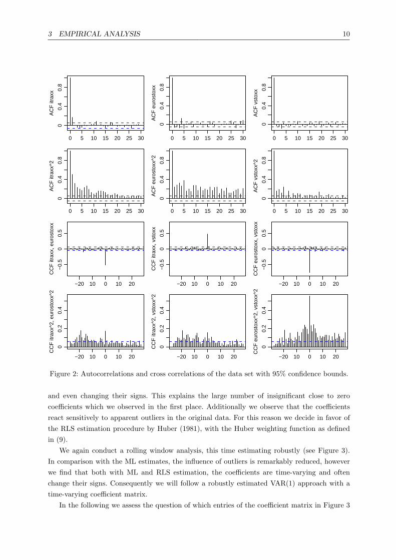
logarithmic differences multiplied by one hundred (see Figure 1). Evidence of simple trends andseasonality was not found. Note, that on the whole iTraxx and Euro Stoxx show counter trends,whereas iTraxx and VStoxx indicate a positive interrelation. The three time series display typicalstylized features such as volatility clustering and at least one structural break, which e.g. in mid2007 is related to the rise of the sub-prime crisis. The characteristics of the time series, e.g. interms of mean and volatility levels, change significantly before and after the outbreak of thecrisis (see Table 1), thereby the biggest structural changes are visible in the iTraxx index. Theestimated corresponding autocorrelation functions of the data and the squared data, as well asthe corresponding cross correlations between the time series can be found in Figure 2. We seesome autocorrelation in the time series, especially within the iTraxx at lag one, however thevalues are rather small. Cross correlations are perceivable only at lag zero. The autocorrelationsand cross correlations in the squared data give rise to the hypothesis of stochastic volatility.

3.2 A VAR Model for the Conditional Mean

In a first step, in order to capture the weak autocorrelation in the data as seen in Figure 2, wemodel the conditional mean of the time series by fitting a VAR model as given by (1) to thedata. In order to determine the model order p, we fit different models up to order p = 10 via MLestimation and calculate the associated information criteria AIC, HQ and SC (see Akaike 1973,1974, Hannan and Quinn, 1979 and Schwarz, 1978). As displayed in Table 2, AIC suggests p = 4,whereas HQ and SC both recommend model order p = 1. We therefore fit a VAR(1) model toour data. When conducting ML estimation of the coefficient matrix Φ we find that six out ofnine coefficients are insignificant. Precisely only the coefficients Φ11, Φ21 and Φ33 are significantat a 90 % confidence level. We also observe, that the coefficient matrix contains mostly verysmall values. In order to gain deeper insight into the vector autoregressive structure of our dataset we therefore conduct a rolling window analysis of the coefficient matrix. We use differentwindows from 25 to 300 days, finding that all coefficients vary over time, some very strongly


Lag

0 5 10 15 20 25 30

00.

40.

8

AC

F it

raxx

Lag

0 5 10 15 20 25 30

00.

40.

8

AC

F e

uros

toxx

Lag

0 5 10 15 20 25 30

00.

40.

8

AC

F v

stox

x

Lag

0 5 10 15 20 25 30

00.

40.

8

AC

F it

raxx

^2

Lag

0 5 10 15 20 25 30

00.

40.

8

AC

F e

uros

toxx

^2

Lag

0 5 10 15 20 25 30

00.

40.

8

AC

F v

stox

x^2

Lag

−20 10 0 10 20

−0.

50

0.5

CC

F it

raxx

, eur

osto

xx

Lag

−20 10 0 10 20

−0.

50

0.5

CC

F it

raxx

, vst

oxx

Lag

−20 10 0 10 20

−0.

50

0.5

CC

F e

uros

toxx

, vst

oxx

−20 10 0 10 20

00.

20.

4

CC

F it

raxx

^2, e

uros

toxx

^2

−20 10 0 10 20

00.

20.

4

CC

F it

raxx

^2, v

stox

x^2

−20 10 0 10 20

00.

20.

4

CC

F e

uros

toxx

^2, v

stox

x^2

Figure 2: Autocorrelations and cross correlations of the data set with 95% confidence bounds.

and even changing their signs. This explains the large number of insignificant close to zerocoefficients which we observed in the first place. Additionally we observe that the coefficientsreact sensitively to apparent outliers in the original data. For this reason we decide in favor ofthe RLS estimation procedure by Huber (1981), with the Huber weighting function as definedin (9).

We again conduct a rolling window analysis, this time estimating robustly (see Figure 3).In comparison with the ML estimates, the influence of outliers is remarkably reduced, howeverwe find that both with ML and RLS estimation, the coefficients are time-varying and oftenchange their signs. Consequently we will follow a robustly estimated VAR(1) approach with atime-varying coefficient matrix.

In the following we assess the question of which entries of the coefficient matrix in Figure 3


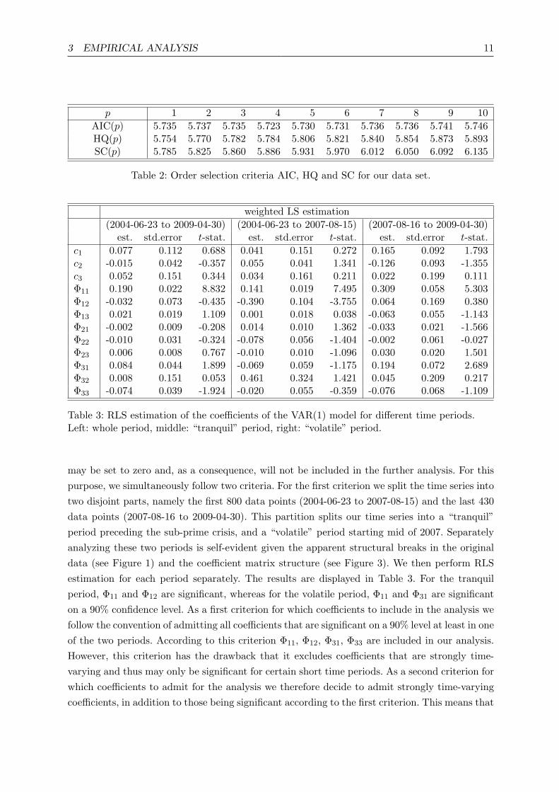
p 1 2 3 4 5 6 7 8 9 10AIC(p) 5.735 5.737 5.735 5.723 5.730 5.731 5.736 5.736 5.741 5.746HQ(p) 5.754 5.770 5.782 5.784 5.806 5.821 5.840 5.854 5.873 5.893SC(p) 5.785 5.825 5.860 5.886 5.931 5.970 6.012 6.050 6.092 6.135

Table 2: Order selection criteria AIC, HQ and SC for our data set.

weighted LS estimation(2004-06-23 to 2009-04-30) (2004-06-23 to 2007-08-15) (2007-08-16 to 2009-04-30)

est. std.error t-stat. est. std.error t-stat. est. std.error t-stat.c1 0.077 0.112 0.688 0.041 0.151 0.272 0.165 0.092 1.793c2 -0.015 0.042 -0.357 0.055 0.041 1.341 -0.126 0.093 -1.355c3 0.052 0.151 0.344 0.034 0.161 0.211 0.022 0.199 0.111Φ11 0.190 0.022 8.832 0.141 0.019 7.495 0.309 0.058 5.303Φ12 -0.032 0.073 -0.435 -0.390 0.104 -3.755 0.064 0.169 0.380Φ13 0.021 0.019 1.109 0.001 0.018 0.038 -0.063 0.055 -1.143Φ21 -0.002 0.009 -0.208 0.014 0.010 1.362 -0.033 0.021 -1.566Φ22 -0.010 0.031 -0.324 -0.078 0.056 -1.404 -0.002 0.061 -0.027Φ23 0.006 0.008 0.767 -0.010 0.010 -1.096 0.030 0.020 1.501Φ31 0.084 0.044 1.899 -0.069 0.059 -1.175 0.194 0.072 2.689Φ32 0.008 0.151 0.053 0.461 0.324 1.421 0.045 0.209 0.217Φ33 -0.074 0.039 -1.924 -0.020 0.055 -0.359 -0.076 0.068 -1.109

Table 3: RLS estimation of the coefficients of the VAR(1) model for different time periods.Left: whole period, middle: “tranquil” period, right: “volatile” period.

may be set to zero and, as a consequence, will not be included in the further analysis. For thispurpose, we simultaneously follow two criteria. For the first criterion we split the time series intotwo disjoint parts, namely the first 800 data points (2004-06-23 to 2007-08-15) and the last 430data points (2007-08-16 to 2009-04-30). This partition splits our time series into a “tranquil”period preceding the sub-prime crisis, and a “volatile” period starting mid of 2007. Separatelyanalyzing these two periods is self-evident given the apparent structural breaks in the originaldata (see Figure 1) and the coefficient matrix structure (see Figure 3). We then perform RLSestimation for each period separately. The results are displayed in Table 3. For the tranquilperiod, Φ11 and Φ12 are significant, whereas for the volatile period, Φ11 and Φ31 are significanton a 90% confidence level. As a first criterion for which coefficients to include in the analysis wefollow the convention of admitting all coefficients that are significant on a 90% level at least in oneof the two periods. According to this criterion Φ11, Φ12, Φ31, Φ33 are included in our analysis.However, this criterion has the drawback that it excludes coefficients that are strongly time-varying and thus may only be significant for certain short time periods. As a second criterion forwhich coefficients to admit for the analysis we therefore decide to admit strongly time-varyingcoefficients, in addition to those being significant according to the first criterion. This means that


Index

200 600 1000

−4

−2

02

4

ΦΦ11

Index

200 600 1000

−4

−2

02

4

ΦΦ12

Index

200 600 1000

−4

−2

02

4

ΦΦ13

Index

200 600 1000

−4

−2

02

4

ΦΦ21

Index

200 600 1000

−4

−2

02

4

ΦΦ22

Index

200 600 1000

−4

−2

02

4

ΦΦ23

200 600 1000

−4

−2

02

4

ΦΦ31

200 600 1000

−4

−2

02

4

ΦΦ32

200 600 1000−

4−

20

24

ΦΦ33

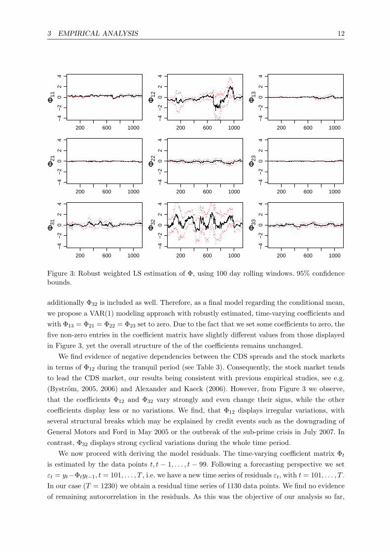
Figure 3: Robust weighted LS estimation of Φ, using 100 day rolling windows. 95% confidencebounds.

additionally Φ32 is included as well. Therefore, as a final model regarding the conditional mean,we propose a VAR(1) modeling approach with robustly estimated, time-varying coefficients andwith Φ13 = Φ21 = Φ22 = Φ23 set to zero. Due to the fact that we set some coefficients to zero, thefive non-zero entries in the coefficient matrix have slightly different values from those displayedin Figure 3, yet the overall structure of the of the coefficients remains unchanged.

We find evidence of negative dependencies between the CDS spreads and the stock marketsin terms of Φ12 during the tranquil period (see Table 3). Consequently, the stock market tendsto lead the CDS market, our results being consistent with previous empirical studies, see e.g.(Bystrom, 2005, 2006) and Alexander and Kaeck (2006). However, from Figure 3 we observe,that the coefficients Φ12 and Φ32 vary strongly and even change their signs, while the othercoefficients display less or no variations. We find, that Φ12 displays irregular variations, withseveral structural breaks which may be explained by credit events such as the downgrading ofGeneral Motors and Ford in May 2005 or the outbreak of the sub-prime crisis in July 2007. Incontrast, Φ32 displays strong cyclical variations during the whole time period.

We now proceed with deriving the model residuals. The time-varying coefficient matrix Φt

is estimated by the data points t, t − 1, . . . , t − 99. Following a forecasting perspective we setεt = yt−Φtyt−1, t = 101, . . . , T , i.e. we have a new time series of residuals εt, with t = 101, . . . , T .In our case (T = 1230) we obtain a residual time series of 1130 data points. We find no evidenceof remaining autocorrelation in the residuals. As this was the objective of our analysis so far,


in this respect the model fit is very good. Cross correlations at lag zero are still perceivable, asthey evidently cannot be captured by the VAR model. However, we still observe characteristicpatterns and structural changes in the residuals, and thus the residual time series is obviouslynot generated by a white noise process. Furthermore, the autocorrelation and cross correlationsplots of the squared residuals on the whole still resemble the ones in Figure 2, which emphasizesthe need for an additional modeling of the covariance structure of our time series.

3.3 A BEKK Model for the Conditional Covariance

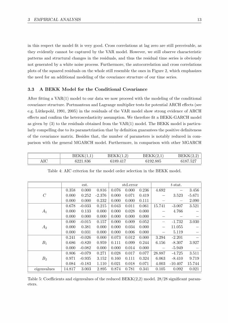
After fitting a VAR(1) model to our data we now proceed with the modeling of the conditionalcovariance structure. Portmanteau and Lagrange multiplier tests for potential ARCH effects (seee.g. Lutkepohl, 1991, 2005) in the residuals of the VAR model show strong evidence of ARCHeffects and confirm the heteroscedasticity assumption. We therefore fit a BEKK-GARCH modelas given by (3) to the residuals obtained from the VAR(1) model. The BEKK model is particu-larly compelling due to its parametrization that by definition guarantees the positive definitenessof the covariance matrix. Besides that, the number of parameters is notably reduced in com-parison with the general MGARCH model. Furthermore, in comparison with other MGARCH

BEKK(1,1) BEKK(1,2) BEKK(2,1) BEKK(2,2)AIC 6221.836 6189.417 6192.885 6187.527

Table 4: AIC criterion for the model order selection in the BEKK model.

est. std.error t-stat.

C0.358 0.000 0.816 0.076 0.000 0.236 4.692 − 3.4560.000 0.252 -2.376 0.000 0.071 0.419 − 3.523 -5.6710.000 0.000 0.232 0.000 0.000 0.111 − − 2.090

A1

0.678 -0.033 0.215 0.043 0.011 0.061 15.741 -3.007 3.5210.000 0.133 0.000 0.000 0.028 0.000 − 4.766 −0.000 0.000 0.000 0.000 0.000 0.000 − − −

A2

0.000 -0.015 0.157 0.000 0.009 0.052 − -1.732 3.0300.000 0.381 0.000 0.000 0.034 0.000 − 11.055 −0.000 0.031 0.000 0.000 0.006 0.000 − 5.119 −

B1

0.241 -0.026 0.000 0.073 0.012 0.000 3.294 -2.201 −0.686 -0.820 0.959 0.111 0.099 0.244 6.156 -8.307 3.9270.000 -0.082 0.000 0.000 0.014 0.000 − -5.949 −

B2

0.806 -0.079 0.271 0.028 0.017 0.077 28.887 -4.725 3.5110.971 -0.935 3.152 0.160 0.111 0.324 6.063 -8.410 9.7190.084 -0.183 1.110 0.021 0.018 0.071 4.003 -10.407 15.744

eigenvalues 14.817 3.003 2.895 0.874 0.781 0.341 0.105 0.092 0.021

Table 5: Coefficients and eigenvalues of the reduced BEKK(2,2) model. 28/28 significant param-eters.


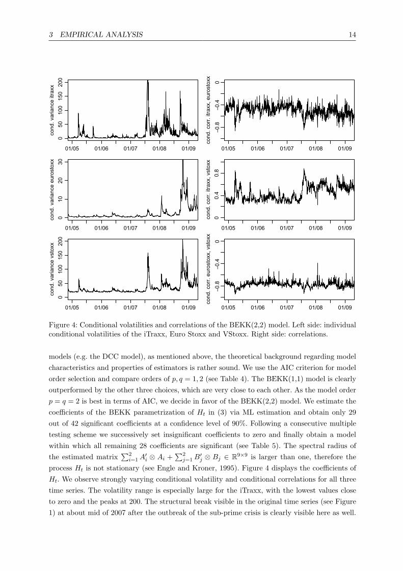
Figure 4: Conditional volatilities and correlations of the BEKK(2,2) model. Left side: individualconditional volatilities of the iTraxx, Euro Stoxx and VStoxx. Right side: correlations.

models (e.g. the DCC model), as mentioned above, the theoretical background regarding modelcharacteristics and properties of estimators is rather sound. We use the AIC criterion for modelorder selection and compare orders of p, q = 1, 2 (see Table 4). The BEKK(1,1) model is clearlyoutperformed by the other three choices, which are very close to each other. As the model orderp = q = 2 is best in terms of AIC, we decide in favor of the BEKK(2,2) model. We estimate thecoefficients of the BEKK parametrization of Ht in (3) via ML estimation and obtain only 29out of 42 significant coefficients at a confidence level of 90%. Following a consecutive multipletesting scheme we successively set insignificant coefficients to zero and finally obtain a modelwithin which all remaining 28 coefficients are significant (see Table 5). The spectral radius ofthe estimated matrix

∑2i=1A

′i ⊗ Ai +

∑2j=1B

′j ⊗ Bj ∈ R9×9 is larger than one, therefore the

process Ht is not stationary (see Engle and Kroner, 1995). Figure 4 displays the coefficients ofHt. We observe strongly varying conditional volatility and conditional correlations for all threetime series. The volatility range is especially large for the iTraxx, with the lowest values closeto zero and the peaks at 200. The structural break visible in the original time series (see Figure1) at about mid of 2007 after the outbreak of the sub-prime crisis is clearly visible here as well.


Figure 5: Residuals after fitting a BEKK(2,2) model to the residuals of the VAR(1) model.

After the break all three volatilities have a higher level on the whole, and vary more strongly.This, again, is particularly evident in the case of the iTraxx index. The correlation betweenthe iTraxx and the Euro Stoxx as well as the Euro Stoxx and the VStoxx is negative, while thecorrelation between the iTraxx and the VStoxx is positive. The conditional correlations betweenthe three time series fluctuate strongly over time. While the correlation between the iTraxx andthe other two indices is stronger after the structural break, the correlation between the EuroStoxx and the VStoxx stays on the same level, which is not surprising, as the values of theVStoxx are calculated on the basis of options on the Euro Stoxx. By its nature the VStoxx istherefore closely linked to the development of the Euro Stoxx.

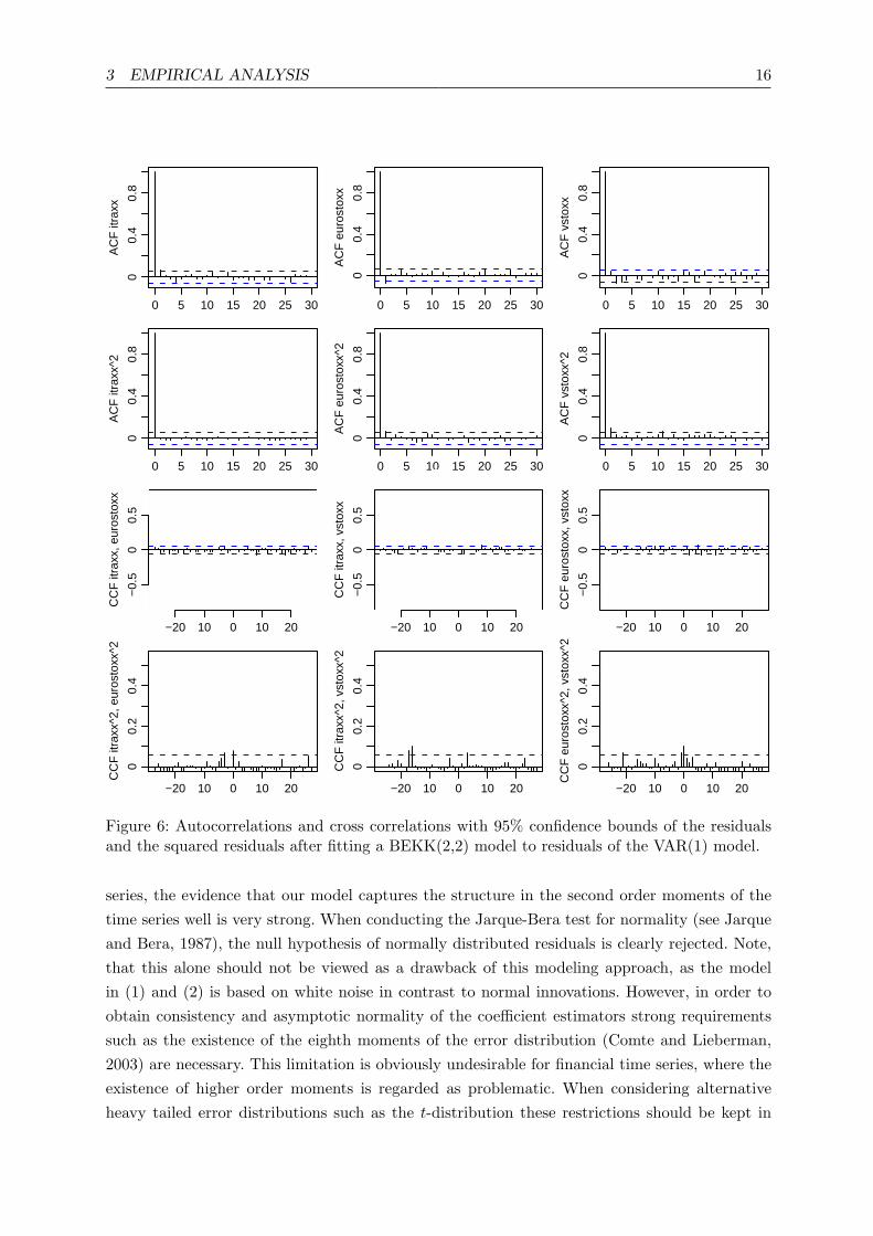
Figure 5 shows the residuals after fitting the BEKK(2,2) model. In comparison with theoriginal data in Figure 1, we can see that much of the previous volatility patterns have vanished,this implies that the BEKK model was able to capture the volatility structure of the data set. Theautocorrelations and cross correlations of the residuals and the squared residuals are displayedin Figure 6. There are no significant auto- and cross correlations left. We conduct portmanteauand Lagrange multiplier tests and find no evidence of remaining ARCH effects. Overall, whenconsidering the test results and the autocorrelations and cross correlations plots of all three time


0 5 10 15 20 25 30

00.

40.

8

AC

F it

raxx

0 5 10 15 20 25 30

00.

40.

8

AC

F e

uros

toxx

0 5 10 15 20 25 30

00.

40.

8

AC

F v

stox

x

0 5 10 15 20 25 30

00.

40.

8

AC

F it

raxx

^2

0 5 10 15 20 25 30

00.

40.

8

AC

F e

uros

toxx

^2

0 5 10 15 20 25 30

00.

40.

8

AC

F v

stox

x^2

−20 10 0 10 20

−0.

50

0.5

CC

F it

raxx

, eur

osto

xx

−20 10 0 10 20

−0.

50

0.5

CC

F it

raxx

, vst

oxx

−20 10 0 10 20

−0.

50

0.5

CC

F e

uros

toxx

, vst

oxx

−20 10 0 10 20

00.

20.

4

CC

F it

raxx

^2, e

uros

toxx

^2

−20 10 0 10 20

00.

20.

4

CC

F it

raxx

^2, v

stox

x^2

−20 10 0 10 20

00.

20.

4

CC

F e

uros

toxx

^2, v

stox

x^2

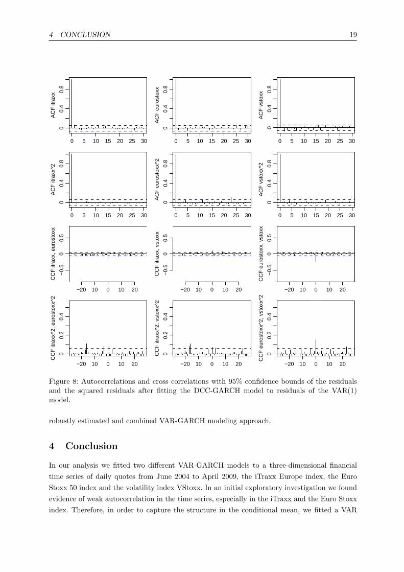
Figure 6: Autocorrelations and cross correlations with 95% confidence bounds of the residualsand the squared residuals after fitting a BEKK(2,2) model to residuals of the VAR(1) model.

series, the evidence that our model captures the structure in the second order moments of thetime series well is very strong. When conducting the Jarque-Bera test for normality (see Jarqueand Bera, 1987), the null hypothesis of normally distributed residuals is clearly rejected. Note,that this alone should not be viewed as a drawback of this modeling approach, as the modelin (1) and (2) is based on white noise in contrast to normal innovations. However, in order toobtain consistency and asymptotic normality of the coefficient estimators strong requirementssuch as the existence of the eighth moments of the error distribution (Comte and Lieberman,2003) are necessary. This limitation is obviously undesirable for financial time series, where theexistence of higher order moments is regarded as problematic. When considering alternativeheavy tailed error distributions such as the t-distribution these restrictions should be kept in


est. std.error t-stat. est. std.error t-stat.ω1 0.141 0.084 1.679 α1 0.270 0.013 20.769ω2 0.027 0.087 0.310 α2 0.133 0.037 3.595ω3 0.914 0.040 22.850 α3 0.065 0.031 2.097a 0.024 0.019 1.263 β1 0.780 0.422 1.848b 0.956 0.031 30.839 β2 0.858 0.025 34.320

β3 0.909 0.032 28.406

Table 6: Coefficients of the DCC model with pi = qi = 1∀ i = 1, . . . , N in (5) and M = N = 1in (6).

mind. When the residuals are found to be skewed, the relevance of the Student distributionmay be questioned. Therefore in this case, skewed distributions with fat tails, such as mixturesof multivariate normal densities or the generalized hyperbolic distribution are more suitablealternative error distributions.

3.4 A DCC Model for the Conditional Covariance

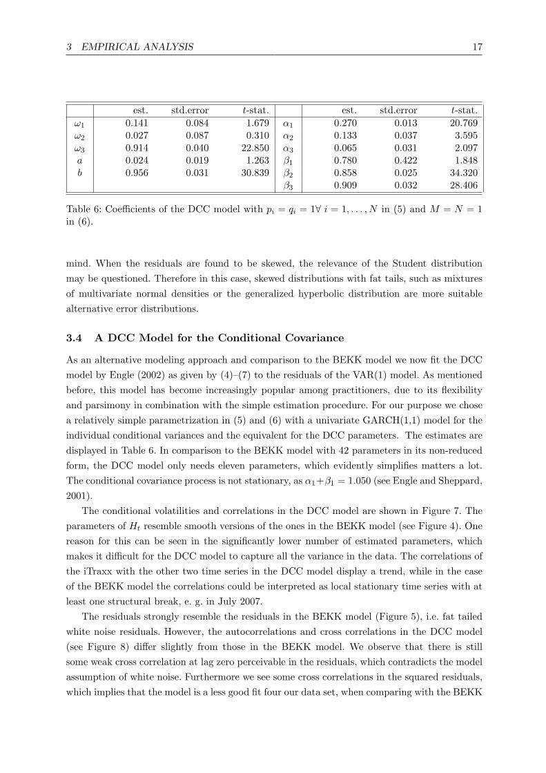
As an alternative modeling approach and comparison to the BEKK model we now fit the DCCmodel by Engle (2002) as given by (4)–(7) to the residuals of the VAR(1) model. As mentionedbefore, this model has become increasingly popular among practitioners, due to its flexibilityand parsimony in combination with the simple estimation procedure. For our purpose we chosea relatively simple parametrization in (5) and (6) with a univariate GARCH(1,1) model for theindividual conditional variances and the equivalent for the DCC parameters. The estimates aredisplayed in Table 6. In comparison to the BEKK model with 42 parameters in its non-reducedform, the DCC model only needs eleven parameters, which evidently simplifies matters a lot.The conditional covariance process is not stationary, as α1+β1 = 1.050 (see Engle and Sheppard,2001).

The conditional volatilities and correlations in the DCC model are shown in Figure 7. Theparameters of Ht resemble smooth versions of the ones in the BEKK model (see Figure 4). Onereason for this can be seen in the significantly lower number of estimated parameters, whichmakes it difficult for the DCC model to capture all the variance in the data. The correlations ofthe iTraxx with the other two time series in the DCC model display a trend, while in the caseof the BEKK model the correlations could be interpreted as local stationary time series with atleast one structural break, e. g. in July 2007.

The residuals strongly resemble the residuals in the BEKK model (Figure 5), i.e. fat tailedwhite noise residuals. However, the autocorrelations and cross correlations in the DCC model(see Figure 8) differ slightly from those in the BEKK model. We observe that there is stillsome weak cross correlation at lag zero perceivable in the residuals, which contradicts the modelassumption of white noise. Furthermore we see some cross correlations in the squared residuals,which implies that the model is a less good fit four our data set, when comparing with the BEKK


01/05 01/06 01/07 01/08 01/09

050

100

150

200

cond

. var

ianc

e itr

axx

01/05 01/06 01/07 01/08 01/09

−0.

8−

0.4

0

cond

. cor

r. it

raxx

, eur

osto

xx

01/05 01/06 01/07 01/08 01/09

010

2030

cond

. var

ianc

e eu

rost

oxx

01/05 01/06 01/07 01/08 01/09

00.

40.

8

cond

. cor

r. it

raxx

, vst

oxx

01/05 01/06 01/07 01/08 01/09

050

100

150

200

cond

. var

ianc

e vs

toxx

01/05 01/06 01/07 01/08 01/09

−0.

8−

0.4

0

cond

. cor

r. e

uros

toxx

, vst

oxx

Figure 7: Conditional volatilities and correlations of the DCC model. Left side: individual con-ditional volatilities of the iTraxx, Euro Stoxx and VStoxx. Right side: correlations.

model in Figure 4. On the other hand the BEKK model has a total number of 42 parameters or28 parameters in its reduced form, which by far exceeds the number of parameters of the DCCmodel. The portmanteau and Lagrange multiplier tests for remaining ARCH effects, as well asthe tests for normality yield the same results as in the case of the BEKK model. Considering ourempirical results when comparing the BEKK with the DCC model we find that the DCC modelin its simplest form produces quite similar variance and correlation estimates, while having onlyone fourth of the parameters the BEKK model has. It is therefore not surprising that the DCCmodel enjoys widespread popularity with practitioners. The parsimony of the DCC approachis particularly compelling when high dimensional vector time series are involved, for instancewhen analyzing stock portfolios with many assets.

It is worth mentioning, that in our empirical study we also compared our VAR-GARCHmodeling approach with a simple MGARCH model, where in a first step we subtracted themean from the original time series, and then in a second step fitted a BEKK versus DCC modelto the data. We found that this model clearly is a less good fit when comparing autocorrelationsand cross correlations of the residuals with Figure 6 and Figure 8. This confirms our time-varying,

4 CONCLUSION 19

0 5 10 15 20 25 30

00.

40.

8

AC

F it

raxx

0 5 10 15 20 25 30

00.

40.

8

AC

F e

uros

toxx

0 5 10 15 20 25 30

00.

40.

8

AC

F v

stox

x

0 5 10 15 20 25 30

00.

40.

8

AC

F it

raxx

^2

0 5 10 15 20 25 30

00.

40.

8

AC

F e

uros

toxx

^2

0 5 10 15 20 25 30

00.

40.

8

AC

F v

stox

x^2

−20 10 0 10 20

−0.

50

0.5

CC

F it

raxx

, eur

osto

xx

−20 10 0 10 20

−0.

50

0.5

CC

F it

raxx

, vst

oxx

−20 10 0 10 20

−0.

50

0.5

CC

F e

uros

toxx

, vst

oxx

−20 10 0 10 20

00.

20.

4

CC

F it

raxx

^2, e

uros

toxx

^2

−20 10 0 10 20

00.

20.

4

CC

F it

raxx

^2, v

stox

x^2

−20 10 0 10 20

00.

20.

4

CC

F e

uros

toxx

^2, v

stox

x^2

Figure 8: Autocorrelations and cross correlations with 95% confidence bounds of the residualsand the squared residuals after fitting the DCC-GARCH model to residuals of the VAR(1)model.

robustly estimated and combined VAR-GARCH modeling approach.

4 Conclusion

In our analysis we fitted two different VAR-GARCH models to a three-dimensional financialtime series of daily quotes from June 2004 to April 2009, the iTraxx Europe index, the EuroStoxx 50 index and the volatility index VStoxx. In an initial exploratory investigation we foundevidence of weak autocorrelation in the time series, especially in the iTraxx and the Euro Stoxxindex. Therefore, in order to capture the structure in the conditional mean, we fitted a VAR

4 CONCLUSION 20

model to the data. We selected order one as recommended by the HQ and SC informationcriteria. In order to account for the apparent outliers in the data, and the strongly varyingentries of the coefficient matrix, we robustly estimated a VAR(1) model with time-dependentcoefficients using RLS estimation. By establishing two criteria for setting insignificant coefficientsto zero we achieved a parsimonious model specification. Our empirical results indicate that theautoregressive coefficients vary strongly with time and even change their signs. Well-knowninterrelations, such as the negative correlation between CDS’ and stocks are lost through thefinancial crisis. We found the model adequate in terms of the conditional mean, however mostof the dependency structure of the time series was captured by the MGARCH models, whichwere fitted to the residuals subsequently.

From the variety of MGARCH modeling approaches developed up to date we chose thewell known BEKK model, which is particularly compelling due to its parametrization that bydefinition guarantees the positive definiteness of the covariance matrix. We fitted a BEKK(2,2)model to the data, the model order being determined by AIC. As a model comparison we choseto fit a DCC model to the data, motivated by its widespread popularity among practitioners.For our purpose we chose a simple model class with a GARCH(1,1) model for the individualconditional variances and the equivalent for the DCC parameters.

We found that the conditional variances and correlations vary strongly with time. The corre-lations between the iTraxx and the Euro Stoxx and the Euro Stoxx and the VStoxx are negative,whereas the correlation between the iTraxx and the VStoxx is positive. The correlations increasesignificantly in absolute values after the outbreak of the financial crisis. The main difference be-tween the two models lies in the smoother variance and correlation estimates in the DCC model.Besides that, the correlations in the DCC model display a trend, whereas in the BEKK modelthe correlations could be interpreted as local stationary time series. Both series of residuals arewhite noise yet not normally distributed.

In terms of the conditional mean, our results extend previous empirical studies, allowingfor robustly estimated, time-varying coefficients. However, to the best of our knowledge, thereare no existing studies of aggregated credit spreads, stocks and stock market volatility in whichthe conditional covariance structure is considered. Therefore our findings offer some of the firstinsights regarding the variance and correlation structure of this data set. We found evidenceof strongly varying conditional variances and correlations, with dependencies increasing afterthe outbreak of the financial crisis. This knowledge opens the door to better decision tools invarious areas, such as asset pricing, portfolio selection, and risk management. The dynamics ofthe financial crisis particularly with regard to the correlations between different asset classesmay hence be understood from a new and more thorough view point.

REFERENCES 21

References

Akaike, H. (1973). Information theory and an extension of the maximum likelihood principle.In B. N. Petrov and F. Csaki (Eds.), 2nd International Symposium on Information Theory,Budapest, pp. 267–281.

Akaike, H. (1974). A new look at the statistical model identification. IEEE Transactions onAutomatic Control 19 (6), 716–723.

Alexander, C. and A. Kaeck (2006). Regimes in CDS spreads: a Markov switching model ofiTraxx Europe indices. ICMA Centre Discussion Papers in Finance, Henley Business School,Reading University.

Bauwens, L., S. Laurent, and J. V. Rombouts (2006). Multivariate GARCH models: a survey.Journal of Applied Econometrics 21 (1), 79–109.

Bollerslev, T. (1986). Generalized autoregressive conditional heteroskedasticity. Journal ofEconometrics 31 (3), 307–327.

Bollerslev, T. (1990). Modelling the coherence in short-run nominal exchange rates: a multivari-ate generalized ARCH model. The Review of Economics and Statistics 72 (3), 498–505.

Bollerslev, T., R. F. Engle, and J. M. Wooldridge (1988). A capital asset pricing model withtime-varying covariances. Journal of Political Economy 96 (1), 116–31.

Brockwell, P. J. and R. A. Davis (1991). Time Series: Theory and Methods. New York: Springer.

Bystrom, H. N. E. (2005). Credit default swaps and equity prices: the iTraxx CDS index market.Working Papers, Department of Economics, Lund University (Lund, Sweden).

Bystrom, H. N. E. (2006). CreditGrades and the iTraxx CDS index market. Financial AnalystsJournal 62 (6), 65–76.

Campbell, K. (1982). Recursive computation of M-estimates for the parameters of a finiteautoregressive process. The Annals of Statistics 10 (2), 442–453.

Caporin, M. and M. McAleer (2008). Scalar BEKK and indirect DCC. Journal of Forecast-ing 27 (6), 537–549.

Caporin, M. and M. McAleer (2009). Do we really need both BEKK and DCC? A tale oftwo covariance models. Documentos del Instituto Complutense de Analisis Economico 0904,Universidad Complutense de Madrid, Facultad de Ciencias Economicas y Empresariales.

Comte, F. and O. Lieberman (2003). Asymptotic theory for multivariate GARCH processes.Journal of Multivariate Analysis 84 (1), 61–84.

REFERENCES 22

Engle, R. F. (1982). Autoregressive conditional heteroscedasticity with estimates of the varianceof United Kingdom inflation. Econometrica 50 (4), 987–1007.

Engle, R. F. (2002). Dynamic conditional correlation: a simple class of multivariate general-ized autoregressive conditional heteroskedasticity models. Journal of Business & EconomicStatistics 20 (3), 339–350.

Engle, R. F. and K. F. Kroner (1995). Multivariate simultaneous generalized ARCH. Econo-metric Theory 11 (1), 122–150.

Engle, R. F., K. F. Kroner, Y. Baba, and D. F. Kraft (1993). Multivariate simultaneous gener-alized ARCH. Economics Working Paper Series 89–57, Department of Economics, Universityof California at San Diego.

Engle, R. F. and K. Sheppard (2001). Theoretical and empirical properties of dynamic con-ditional correlation multivariate GARCH. NBER Working Paper 8554, National Bureau ofEconomic Research.

Ericsson, J., K. Jacobs, and R. A. Oviedo (2009). The determinants of credit default swappremia. Journal of Financial and Quantitative Analysis 44 (1), 109–132.

Hamilton, J. (1994). Time Series Analysis. Princeton University Press.

Hannan, E. J. (1970). Multiple Time Series. New York: John Wiley & Sons.

Hannan, E. J. and B. G. Quinn (1979). The determination of the order of an autoregression.Journal of the Royal Statistical Society, Series B (41), 190–195.

Houweling, P. and T. Vorst (2005). Pricing default swaps: empirical evidence. Journal ofInternational Money and Finance 24 (8), 1200–1225.

Huber, P. J. (1981). Robust Statistics. New York: John Wiley & Sons.

Jarque, C. M. and A. K. Bera (1987). A test for normality of observations and regressionresiduals. International Statistical Review 55, 163–172.

Li, W. K. and Y. V. Hui (1989). Robust multiple time series modelling. Biometrika 76 (2),309–315.

Li, W. K., S. Ling, and M. McAleer (2002). Recent theoretical results for time series modelswith GARCH errors. Journal of Economic Surveys 16 (3), 245–269.

Lutkepohl, H. (1991). Introduction to Multiple Time Series Analysis. Berlin: Springer-Verlag.

Lutkepohl, H. (2005). New Introduction to Multiple Time Series Analysis. Berlin: Springer-Verlag.

REFERENCES 23

Newey, W. K. and D. McFadden (1994). Large sample estimation and hypothesis testing. InR. F. Engle and D. McFadden (Eds.), Handbook of Econometrics, Volume 4, pp. 2111–2245.Amsterdam: Elsevier Science.

Norden, L. and M. Weber (2009). The comovement of credit default swap, bond and stockmarkets: an empirical analysis. European Financial Management 15 (3), 529–562.

Schwarz, G. (1978). Estimating the dimension of a model. Annals of Statistics (6), 461–464.

Sims, C. A. (1972). Money, income and causality. American Economic Review 62 (4), 540–52.

Sims, C. A. (1980). Macroeconomics and reality. Econometrica 48 (1), 1–48.

Sougne, C., C. Heuchenne, and G. Hubner (2008). The determinants of CDS prices: an industry-based investigation. In N. Wagner (Ed.), Credit Risk, pp. 85–96. Boca Raton: Chapman &Hall CRC.

equities, credits and volatilities: a multivariate analysis - mediatum

Documents