equity premium predictability over the business cycle

Discussion PaperDeutsche BundesbankNo 25/2021

Equity premium predictabilityover the business cycle

Emanuel Moench(Deutsche Bundesbank, Goethe University Frankfurt and CEPR)

Tobias Stein(Deutsche Bundesbank and Goethe University Frankfurt)

Discussion Papers represent the authors‘ personal opinions and do notnecessarily reflect the views of the Deutsche Bundesbank or the Eurosystem.

Editorial Board: Daniel Foos Stephan Jank Thomas Kick Martin Kliem Malte Knüppel Christoph Memmel Panagiota Tzamourani

Deutsche Bundesbank, Wilhelm-Epstein-Straße 14, 60431 Frankfurt am Main, Postfach 10 06 02, 60006 Frankfurt am Main

Tel +49 69 9566-0

Please address all orders in writing to: Deutsche Bundesbank, Press and Public Relations Division, at the above address or via fax +49 69 9566-3077

Internet http://www.bundesbank.de

Reproduction permitted only if source is stated.

ISBN 978–3–95729–833–1 ISSN 2749–2958

Non-technical summary

Research Question

Is the equity premium predictable? This question has been the subject of long

debate in finance. A common finding which emerges from the literature is that

predictability primarily arises around recessions. Another strand of the literature

has documented that information in the yield curve can be used to predict reces-

sions. In this paper we study whether recession probabilities implied by models

based on yield curve information improve equity premium predictability.

Contribution

We show that the U.S. equity premium follows a pronounced v-shape pattern

around the beginning of recessions. It sharply drops into negative territory just

before business cycle peaks and then strongly recovers as the recession unfolds.

Recessions are preceded by an inverted yield curve and can be well predicted

using yield curve information. Using probit models, we confirm that the term

spread predicts the beginning of recessions well, and that lags and backward-

looking averages of the term spread further improve the predictability at short

horizons. Second, we show that these model-implied recession probabilities also

have strong predictive power for the U.S. equity premium.

Results

We document that equity premium forecasts based on recession probabilities cor-

rectly anticipate negative stock returns heading into recessions and positive returns

in expansions. We further document a structural break in the mean of the term

spread in 1982 which helps explain why related studies find relatively muted re-

cession signals in recent decades. When correcting for this structural break, both

recession and equity premium forecasts further improve, outperforming other re-

cently proposed predictor variables. Our paper thus provides further evidence for

the strong link between the business cycle and the equity premium. More specifi-

cally, it shows that information in the yield curve can be used to time the equity

market.

Nichttechnische Zusammenfassung

Fragestellung

Kann die Eigenkapitalrisikopramie vorhergesagt werden? Diese Frage ist ein zen-

traler Bestandteil der finanzwirtschaftlichen Forschung. In diversen Studien wird

berichtet, dass die Risikopramie lediglich im zeitlichen Umfeld von Rezessionen

prognostiziert werden kann. Aus anderen Studien geht zudem hervor, dass Infor-

mationen in der Zinsstrukturkurve geeignet sind, um Rezessionen vorherzusagen.

In dieser Arbeit nutzen wir diese beiden Erkenntnisse, indem wir mit Hilfe der

Zinsstrukturkurve zunachst Rezessionswahrscheinlichkeiten bestimmen, mit denen

wir dann die Risikopramie vorhersagen.

Beitrag

Die amerikanische Eigenkapitalrisikopramie weist ein deutliches v-Muster zu Be-

ginn von Rezessionen auf. Die Risikopramie wird typischerweise kurz vor Beginn

einer Rezession negativ und erholt sich dann im Laufe der Rezession. Wir ver-

wenden ein Probit-Modell mit erklarenden Variablen aus der Zinsstrukturkurve

und zeigen, dass der Beginn von Rezessionen gut vorhergesagt werden kann. Die

Vorhersagegute verbessert sich signifikant, wenn sowohl verzogerte als auch gemit-

telte Vergangenheitswerte des Zinsspreads berucksichtigt werden. In einem zweiten

Schritt zeigen wir, dass die vorhergesagten Rezessionswahrscheinlichkeiten eben-

falls die Eigenkapitalrendite vorhersagen konnen.

Ergebnisse

Die 2-Schritt-Methode ist geeignet, um sowohl negative Risikopramien zu Beginn

einer Rezession als auch positive Risikopramien wahrend eines Aufschwungs abzu-

bilden. Des Weiteren zeigt die Analyse, dass der durchschnittliche Zinsspread einen

Strukturbruch im Jahr 1982 aufweist. Eine Berucksichtigung des Strukturbruchs

im Probit-Modell verbessert die Prognosegute sowohl fur Rezessionen als auch fur

Risikopramien. Grundsatzlich konnen wir feststellen, dass es einen ausgepragten

Zusammenhang zwischen Risikopramie und Konjunkturzyklus gibt und dass die

Zinsstrukturkurve daher wichtige Informationen uber die zukunftige Entwicklung

der Risikopramie liefern kann.

Deutsche Bundesbank Discussion Paper No 25/2021

Equity premium predictability over thebusiness cycle*

Emanuel Moench�

Deutsche Bundesbank, Goethe University Frankfurt, CEPR

Tobias Stein�

Deutsche Bundesbank, Goethe University Frankfurt

Abstract

The equity premium follows a pronounced v-shape pattern around the be-ginning of recessions. It sharply drops into negative territory just beforebusiness cycle peaks and then strongly recovers as the recession unfolds.Recessions are preceded by an inverted yield curve. Thus probit modelsusing the term spread as predictor time the beginning of recessions well.We show that such model-implied recession probabilities strongly improveequity premium prediction out-of-sample. We document a structural breakin the mean of the term spread in 1982. When correcting for this break,the forecast performance further strengthens, outperforming other recentlyproposed benchmark predictors.

Keywords: Recession predictability, return predictability, business cycle,probit model, term spread

JEL classification: E32, E37, C53, G11, G17.

*The views expressed in this paper are those of the authors and do not necessarily coincidewith the views of the Deutsche Bundesbank or the Eurosystem.

�Email: [email protected]�Email: [email protected]

1 Introduction

Whether the equity premium is predictable has been the subject of long debatein finance. A large literature documents in-sample predictability using a host offinancial and economic variables such as valuation ratios, the default spread or theconsumption-wealth ratio as predictors (see, e.g. Fama and French (1988), Camp-bell and Shiller (1988), Lettau and Ludvigson (2001)). However, in an influentialpaper Welch and Goyal (2008) show that none of the proposed predictors wouldhave consistently outperformed a simple historical average return out-of-sample.Since then, a growing literature proposes alternative predictors and forecastingmethods which appear to provide superior statistical predictability relative to thehistorical average benchmark, see Rapach and Zhou (2013) for an overview.1 Acommon finding is that predictability primarily arises around recessions.

This is consistent with a related literature suggesting that expected equity returnsvary over the business cycle (e.g. Fama and French (1989), Ferson and Harvey(1991), Cochrane (2007), Campbell and Diebold (2009)). Lustig and Verdelhan(2012) document significant variation in realized excess returns around recessions,showing that they are negative at the business cycle peak and then sharply riseover following quarters. This is confirmed by Figure 1 which depicts the forward-looking arithmetic mean and median of the U.S. log equity premium over differenttime windows around the ten NBER recessions for the period from March 1951to December 2019. The equity premium is mostly negative but relatively volatilefor the one-month and three-month window around the beginning of recessions.However, a clear v-shape emerges for the cumulative six- and twelve-month aheadhorizons, highlighting that equity returns are sharply negative around businesscycle peaks but strongly recover thereafter.

Table 1 presents moments of the annualized log equity premium over the businesscycle for the same 70-year period. The total annual equity premium was 6.3%with a standard deviation of 14.3%, implying a Sharpe ratio of 0.4. Focusingonly on NBER expansions, the equity premium amounted to 8.4% with an an-nualized Sharpe ratio of 0.6. In recessions, it was negative at -5.9%. Zooming in

1Among others, recently proposed predictors include the output gap (Cooper and Priest-ley, 2009), short interest (Rapach, Ringgenberg, and Zhou, 2016), industrial electricity usage(Da, Huang, and Yun, 2017), gold-to-platinum ratio (Huang and Kilic, 2019), variance risk pre-mium (Pyun, 2019), and investor attention (Chen, Tang, Yao, and Zhou, 2020). Methodologicalcontributions include non-negativity constraints (Campbell and Thompson, 2008), combinationforecasts (Rapach, Strauss, and Zhou, 2010), time-varying coefficient models (Dangl and Halling,2012), principal component analysis (Neely, Rapach, Tu, and Zhou, 2014), economic constraints(Pettenuzzo, Timmermann, and Valkanov, 2014), and machine learning techniques (Gu, Kelly,and Xiu, 2020).

1

h = 1 h = 3

−20 −10 0 10 20

−5 %

0 %

5 %

MeanMedian

−20 −10 0 10 20

−10 %

0 %

10 %

MeanMedian

h = 6 h = 12

−20 −10 0 10 20

−10 %

0 %

10 %

MeanMedian

−20 −10 0 10 20

−15 %

0 %

15 %

MeanMedian

Figure 1: Log equity premium around business cycle peaksThis figure presents the arithmetic average and median of the (cumulative) log equity premiumaround the 10 recessions in the sample from 1951:3 to 2019:12. The equity premium is thedifference between value-weighted returns on the S&P 500 index (including dividends) and the

Treasury bill rate. The vertical axis depicts∑h−1

j=0 rt+j for t = −24, . . . ,−1, 0, 1, . . . , 24, wherebyrt+j is the log equity premium in month t + j. The horizontal axis displays the 24 monthsbefore and after a business cycle peak - with t = 0 referring to the first month of a NBER-datedrecession. Results are shown for h = 1, 3, 6, 12.

around business cycle peaks, we see that the equity premium tended to be stronglynegative during the six months before and after the business cycle peak, with an-nualized values of almost -10% and -18%, respectively. Hence, the stock marketon average incurs large losses in the one-year window around the beginning ofrecessions. While it tends to recover in the subsequent months, on average it onlygains an annualized 1.5% six to eleven months after the peak. The last two rows inTable 1 show the annualized log equity premium for samples that exclude the 12months and the 24 months around the beginning of recessions, respectively. When

2

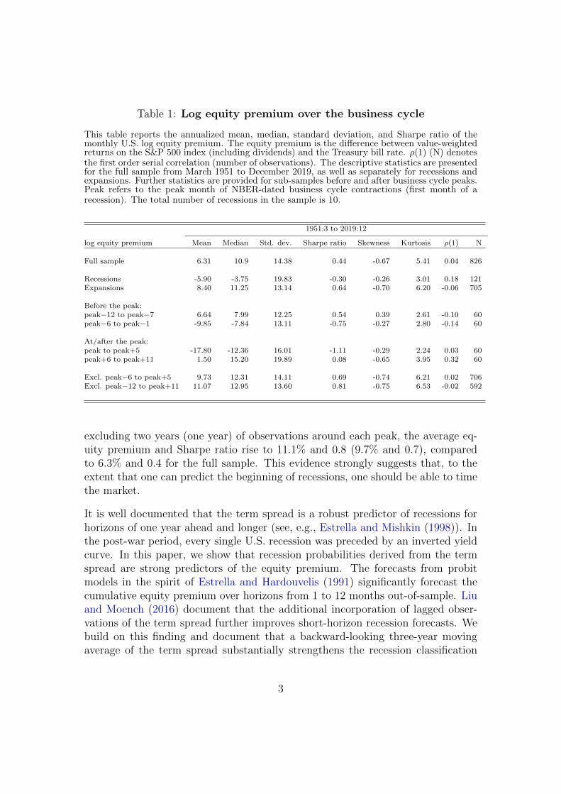
Table 1: Log equity premium over the business cycle

This table reports the annualized mean, median, standard deviation, and Sharpe ratio of themonthly U.S. log equity premium. The equity premium is the difference between value-weightedreturns on the S&P 500 index (including dividends) and the Treasury bill rate. ρ(1) (N) denotesthe first order serial correlation (number of observations). The descriptive statistics are presentedfor the full sample from March 1951 to December 2019, as well as separately for recessions andexpansions. Further statistics are provided for sub-samples before and after business cycle peaks.Peak refers to the peak month of NBER-dated business cycle contractions (first month of arecession). The total number of recessions in the sample is 10.

1951:3 to 2019:12

log equity premium Mean Median Std. dev. Sharpe ratio Skewness Kurtosis ρ(1) N

Full sample 6.31 10.9 14.38 0.44 -0.67 5.41 0.04 826

Recessions -5.90 -3.75 19.83 -0.30 -0.26 3.01 0.18 121Expansions 8.40 11.25 13.14 0.64 -0.70 6.20 -0.06 705

Before the peak:peak−12 to peak−7 6.64 7.99 12.25 0.54 0.39 2.61 -0.10 60peak−6 to peak−1 -9.85 -7.84 13.11 -0.75 -0.27 2.80 -0.14 60

At/after the peak:peak to peak+5 -17.80 -12.36 16.01 -1.11 -0.29 2.24 0.03 60peak+6 to peak+11 1.50 15.20 19.89 0.08 -0.65 3.95 0.32 60

Excl. peak−6 to peak+5 9.73 12.31 14.11 0.69 -0.74 6.21 0.02 706Excl. peak−12 to peak+11 11.07 12.95 13.60 0.81 -0.75 6.53 -0.02 592

excluding two years (one year) of observations around each peak, the average eq-uity premium and Sharpe ratio rise to 11.1% and 0.8 (9.7% and 0.7), comparedto 6.3% and 0.4 for the full sample. This evidence strongly suggests that, to theextent that one can predict the beginning of recessions, one should be able to timethe market.

It is well documented that the term spread is a robust predictor of recessions forhorizons of one year ahead and longer (see, e.g., Estrella and Mishkin (1998)). Inthe post-war period, every single U.S. recession was preceded by an inverted yieldcurve. In this paper, we show that recession probabilities derived from the termspread are strong predictors of the equity premium. The forecasts from probitmodels in the spirit of Estrella and Hardouvelis (1991) significantly forecast thecumulative equity premium over horizons from 1 to 12 months out-of-sample. Liuand Moench (2016) document that the additional incorporation of lagged obser-vations of the term spread further improves short-horizon recession forecasts. Webuild on this finding and document that a backward-looking three-year movingaverage of the term spread substantially strengthens the recession classification

3

ability of the term spread by reducing false positives and better timing the begin-ning of recessions. The improved recession predictability goes hand in hand withstrong improvements in equity premium forecasts: especially at short horizons,equity premium predictability is substantially enhanced by including a backward-looking moving average of the term spread into the probit models. Our resultshighlight the close link between recession expectations and equity market returns.Specifically, we show that the v-shaped pattern of excess returns around businesscycle peaks is well captured by real-time recession probability forecasts based on in-formation in the yield curve. Our findings are thus in line with Rapach et al. (2010)and Dangl and Halling (2012) who find that the predictive power of combinationforecasts and time-varying coefficient models primarily arises from business-cyclevariation in the equity premium. Importantly, however, equity premium forecastsbased on recession probabilities outperform the historical average benchmark alsoin expansions. The reason is that by correctly anticipating low equity market re-turns heading into recessions, they also correctly predict higher returns in businesscycle booms.

Several authors have argued that the probit model for forecasting recessions suffersfrom a structural break (see, e.g., Chauvet and Potter (2002, 2010)). We indeeddocument strong evidence for a structural break in the mean of the term spread in1982 and show that it would have been possible for investors to identify this breakin real-time a few years after it occurred. We follow Lettau and Van Nieuwerburgh(2008) and Pesaran and Timmermann (2007) and apply four different methods tocorrect for the break in the term spread. All further improve the out-of-sampleR2 for forecasting the equity premium. This improvement is partly due to thefact that the real-time break-corrected recession probabilities better predict thebeginning of the 2001 and 2008-2009 recessions.

In terms of predictive ability our approach outperforms other recently proposedpredictors including “short interest” of Rapach et al. (2016) and the “gold-to-platinum” ratio of Huang and Kilic (2019). The out-of-sample R2 is as high as 3%for monthly forecasts and often higher than 10% for cumulative one-year aheadforecasts. Moreover, we perform an asset allocation exercise for a mean-varianceinvestor who invests in the equity market and the risk-free rate. This exercisereveals an excellent market timing ability of recession probability forecasts, whichis even more pronounced for the break-correction methods. The models signal torun down equity exposure before the onset of recessions when the yield curve flat-tens and to re-enter the market toward the end of recessions when the yield curvesteepens. An investor who forecasts with (break-corrected) recession probabilitiesincreases the Sharpe ratio to around 0.85 compared to 0.50 for the buy-and-holdinvestor. Using a VAR-based decomposition in the spirit of Campbell (1991), we

4

find that the predictability is driven by both higher anticipated discount rates andlower expected future dividends, consistent with countercyclical risk premia. Wealso show that our results are robust to taking into account transaction costs andthat model-implied recession probabilities predict the equity premium in othercountries.

In a related recent paper, Gomez-Cram (2021) studies one-month ahead equity pre-mium predictability over the business cycle. Consistent with his results, we findthat stock returns are negative at the beginning of recessions and that businesscycle variables help to time these periods. Despite this broad similarity, there area number of important differences between our and his paper. First, while Gomez-Cram (2021) studies only one-month ahead forecasts, we predict equity returnsalso over longer horizons. Second and more importantly, we combine the recessionand equity premium prediction literatures by directly using recession probabilityforecasts to forecast equity returns, while Gomez-Cram (2021) uses a state-spacemodel to link expected excess equity returns to the business cycle. He estimates acommon growth component from real-time data of nine U.S. macroeconomic vari-ables related to real output, income, employment, consumer spending, investment,and inflation. We instead confirm that the term spread is a robust leading indica-tor of recessions and strongly improves equity premium forecasts. Related to ourfinding Andreasen, Engsted, Møller, and Sander (2020) show that the yield spreadbetter predicts bond risk premiums when conditioning on the business cycle.

The paper proceeds as follows. Section 2 summarizes the data used. Section 3presents the main results, focusing first on the recession probability forecasts andthen on the equity premium prediction using model-implied recession probabilities.Section 4 provides additional robustness checks and Section 5 concludes.

2 Data

We obtain data on the equity premium and term spread from Amit Goyal’s home-page.2 The equity premium is computed as the continuously compounded logreturn on the S&P 500 index, including dividends, minus the Treasury bill rate(Welch and Goyal, 2008). The term spread (TMS) is calculated as the differencebetween the long-term government bond yield and the Treasury bill rate. Theyields are taken from Ibbotson’s Stocks, Bonds, Bills, and Inflation Yearbook andhave a maturity of approximately 20 years (Ibbotson and Sinquefield, 1976). Ourdata set consists of monthly observations from March 1951 to December 2019.We start our analysis in March 1951 after the Treasury-Federal Reserve Accord

2http://www.hec.unil.ch/agoyal/

5

http://www.hec.unil.ch/agoyal/

- which laid the foundation for an independent monetary policy (Lacker, 2001).During World War II and the six years afterwards the Fed was tasked to supportthe financing requirements of the Treasury by stabilizing long-term interest rates(Eichengreen and Garber, 1991; Carlson and Wheelock, 2014). Hence, we beginour analysis after this extraordinary period of pegged interest rates. The busi-ness cycle chronology with classifications into expansions and recessions is takenfrom the National Bureau of Economic Research (NBER). A business cycle peakis defined to be the first month of a recession. We start our pseudo out-of-sampleforecasting exercise in 1980 when the Business Cycle Dating Committee of theNBER began to release timely announcements of its business cycle classifications.

3 Empirical results

This section provides our empirical results. In Sections 3.1 and 3.2, we first confirmthe ability of probit models along the lines of Estrella and Mishkin (1998) to predictNBER recessions. We show that the forecast performance of the standard probitmodel using the term spread as the only explanatory variable strongly improveswhen lagged information about the term spread is added. We then documentin Section 3.3 that the recession probability forecasts implied by probit modelshave strong predictive power for the U.S. equity premium. In Section 3.4, wecompare the results to OLS regressions based on term spread information. InSection 3.5, we provide evidence for a structural break in the mean of the termspread in 1982, and show that this break could have been identified in real-time.We then show in Sections 3.6 and 3.7 that break-correction methods can furtherimprove recession and equity premium forecasts. In Section 3.8, we perform anasset allocation exercise showing that the recession forecasts based on informationin the yield curve significantly improve market timing. In Section 3.9, we extendour analysis to characteristics portfolios. Finally, in Section 3.10 we show thatestimated recession probabilities forecast the equity premium by predicting higherdiscount rates and lower future dividends.

3.1 Predicting recessions

In this section we are interested in predicting U.S. recessions as classified by theNBER Business Cycle Dating Committee. The literature typically distinguishesbetween the probability of a recession in exactly h months and the probability ofa recession within the next h months. Here, we focus on the latter, as we aim toforecast cumulative log equity premiums over the next h months in later sections;for similar definitions see Wright (2006) and Johansson (2018). More precisely,let Yt+1:t+h = 1 if the NBER has classified at least one month between t + 1 and

6

t+h as a recession. We follow common practice and assume that Yt+1:t+h is basedon a latent variable Y ∗t+1:t+h where Yt+1:t+h = 1 for Y ∗t+1:t+h ≥ 0 and Yt+1:t+h = 0for Y ∗t+1:t+h < 0. The latent variable is assumed to follow a (multivariate) linearregression model:

Y ∗t+1:t+h = X′

tβ + εt+1:t+h, (1)

Pr[Yt+1:t+h = 1|Xt

]= Φ

[X′

tβ], (2)

where X′t = (1, x1,t, . . . , xp,t)

′is the 1 × (p + 1) vector of predictor variables in-

cluding the intercept, β is the (p+ 1)× 1 vector of coefficients, and εt+1:t+h is theerror term. Further, Φ

[·]

is the cumulative distribution function of the standardnormal distribution and Pr denotes probability. Let pt+1:t+h be the out-of-sampleforecast for Pr

[Yt+1:t+h = 1

]based on information contained in Xt. We follow

Jacobsen, Marshall, and Visaltanachoti (2019) and account for the fact that theNBER typically publishes business cycle classifications with a substantial delay byestimating the β coefficients with information up to t− 24. This is a conservativechoice as other authors (see, e.g., Kauppi and Saikkonen (2008)) only account fora delay of one year.3 The sample with T observations is split into an in-sampleestimation period of M months and an out-of-sample period of T −M months.We only use data that are available in real-time mimicking as closely as possiblethe information an investor would have had.

In their seminal paper Estrella and Hardouvelis (1991) show that an invertedyield curve is a strong predictor of recessions and future real economic activity.They find that a decline of the term spread is associated with an increase in theprobability of a recession four quarters ahead, and that this predictability is notincorporated in other variables such as lagged inflation, lagged real output growth,and survey data. Estrella and Mishkin (1998) complement this finding by compar-ing the predictive power of the term spread with financial variables such as stockprices and other spreads, as well as monetary aggregates. While some alternativepredictors are useful over one- to three-quarter horizons, it is the term spread thatpredicts best over horizons of one-year and longer. Moreover, the binary modelsfor recessions are found to be more stable than continuous models for economicgrowth (Estrella, Rodrigues, and Schich, 2003), and the relation is also present inother countries including Germany, Japan, and the U.K. (Bernard and Gerlach,1998). Wheelock and Wohar (2009) provide a comprehensive survey of the ability

3The longest delay in our sample was 21 months: the NBER announced the November 2001business cycle trough on July 17, 2003. Results are very similar when we use information up tot− 12.

7

of the term spread to predict recessions.4

The observed predictability of an inverted or flat yield curve for future recessionsis in line with counter-cyclical monetary policy: if the central bank tightens mone-tary policy by raising short-term interest rates, the yield curve tends to flatten andthe economy slows down (Estrella et al., 2003). Estrella (2005) demonstrates thismechanism in a rational expectations model where the monetary policy regimeand the reaction function are key determinants for the predictive power of theterm spread. More recently, Adrian, Estrella, and Shin (2019) argue that thepredictive power of the term spread for future economic activity may result fromactive balance sheet management of financial intermediaries. If the liabilities ofintermediaries are of shorter maturity than their loans, then a narrowing of theinterest margin has a negative effect on the profitability of the marginal loan. As aresult, they reduce the supply of credit. Following this logic, a decrease in the termspread has a negative effect on real activity and thus offers a causal mechanismfor its strong forecasting power.

In what follows, we focus on the simple probit model using (transformations of)the term spread as input. The first model only includes a constant and the termspread as predictors - this is the model of Estrella and Hardouvelis (1991). Itis well known that this model performs well for forecast horizons of one to twoyears, with only weak predictability for shorter horizons. More recently, Liu andMoench (2016) show that the short-horizon forecasts substantially improve whenadding lagged observations of the term spread. Building on this, the second modelincludes the term spread lagged by six months as an additional predictor. As wewill see below, the recession probabilities implied by the two models closely trackthe dynamics of the term spread and thus tend to be quite volatile. This implies anumber of false positive signals about impending recessions. To address this issue,we also consider a specification that includes a constant, the term spread, as wellas a backward-looking three-year moving average of the term spread (MA-TMS)which we construct as 1

36

∑35j=0TMSt−j. We show in the Online Appendix C that

our results are robust to the length of the moving average window.

4Additionally, the literature has studied the predictive power of other variables and methodsin detail. Fornaro (2016) analyzes the performance of a probit model with large-dimensionaldatasets and Bayesian shrinkage. The model performs well over short-horizons and generatessmoother forecasts than benchmark models. Several articles document forecasting gains byincluding credit data like credit spreads, credit growth, and illiquidity measures (Chen, Chou, andYen, 2016; Ponka, 2017; Mihai, 2020), as well as by including sentiment variables (Christiansen,Eriksen, and Møller, 2014). Similarly, there is increasing interest in whether daily and weeklydata can improve monthly recession forecasts - for example in MIDAS regressions (Galvao andOwyang, 2020).

8

1950 1960 1970 1980 1990 2000 2010 2020

−4

−3

−2

−1

01

2

TMStMA−TMSt

Figure 2: Term spread and moving average term spreadThis figure presents the term spread (dashed line) and the moving average term spread (solidline), whereby the latter is the moving average of past three-year observations of the term spread.The time series are normalized to a mean of zero and a standard deviation of one. The sampleis 1951:3 to 2019:12 and shaded areas indicate NBER-dated recession periods.

Figure 2 superimposes TMS and MA-TMS. While the local minima of the termspread usually lead the beginning of recessions by several months, the movingaverage term spread reaches its troughs often just before the onset of recessions.Moreover, the smoothed series averages out some local minima that are not fol-lowed by recessions. The smoothing thus emphasizes lower frequency componentsof the term spread which appear to be more relevant for signaling recessions. Wewill indeed show below that the incorporation of lagged and averaged term spreadinformation into the probit model significantly enhances short horizon forecasts.

Figure 3 shows the out-of-sample recession probability forecasts for the three mod-els from 1980:1 to 2019:12. Several points are noteworthy. First, the model withonly a constant and the term spread performs relatively poorly for h = 1 and h = 3,with several false positives and no pronounced differences between expansions andrecessions since the mid-1980s. The performance for this model gradually increasesin the forecast horizon. This is consistent with the prior literature which has docu-mented an improved recession prediction with the term spread for horizons beyondsix months. Second, the models adding lagged term spread information performsubstantially better for short-horizon forecasts, where the model with the moving

9

average term spread implies substantially smoother recession probabilities. Thisis in line with Rudebusch, Sack, and Swanson (2007) who show that the one-yearlagged term premium predicts future GDP growth, and that differences ratherthan levels of the expectations component and term premium matter more forforecasting real output growth. The finding that lagged observations of the termspread improve recession predictability is consistent with monetary policy affect-ing the economy with a delay of a few quarters (Rudebusch and Williams, 2009).

Third, the recession probabilities in the 1990s and 2000s are less pronounced com-pared to the probabilities in the early 1980s - with values rarely exceeding 50%even in recessions. Similarly, Estrella et al. (2003) document that the signal of themodels was weaker in the 1990-91 recession compared to the early 1980s. Kauppiand Saikkonen (2008) also document - using probit models with lagged dependentvariables - that the 1990-91 and 2001 recessions were difficult to predict. Thispattern is not unique to models using the term spread as predictor, the lack ofpredictability is also documented for models with larger sets of predictors (Hamil-ton, 2011; Fornaro, 2016). We show in Section 3.5 that the weaker recession signalsresult from a structural break in the mean of the term spread in the early 1980s.The probabilities are considerably stronger when this break is accounted for.

3.2 Forecast evaluation

We follow the recession prediction literature and use the quadratic probabilityscore (QPS), the logarithm score (LS) and the diagonal elementary score (DES)to formally evaluate the accuracy of recession probability forecasts.5 Perfect clas-sification ability results in values of zero for all three scores; otherwise they havepositive values, with higher values indicating poorer forecast performance, see,e.g., Nyberg (2013); Christiansen et al. (2014); Fornaro (2016) for recent applica-tions. The loss function of LS penalizes large forecast errors more heavily than theloss function of QPS (Diebold and Rudebusch, 1989). Galvao and Owyang (2020)argue that the loss functions of LS and DES are more suitable in the contextof rare events such as recessions. We further calculate the out-of-sample pseudoR2 (Estrella, 1998) and the area under the receiver operating characteristic curve(AUROC). While the QPS, LS and DES metrics evaluate the model accuracy, theAUROC is a metric to evaluate the classification ability - here into recessions andexpansions - of a forecasting model. A perfect classifier has an AUROC of one anda coin-toss classifier has an AUROC of 0.5; for further details see Berge and Jorda(2011).

Table 2 presents values of the QPS, LS, DES, pseudo R2 and AUROC for the

5Details on the estimation of all statistics in this section are provided in the Online Appendix.

10

h = 1 h = 3

1980 1990 2000 2010 2020

0.0

0.2

0.4

0.6

0.8

1.0

TMStTMSt and TMSt−6TMSt and MA−TMSt

1980 1990 2000 2010 2020

0.0

0.2

0.4

0.6

0.8

1.0


h = 6 h = 12

1980 1990 2000 2010 2020

0.0

0.2

0.4

0.6

0.8

1.0


1980 1990 2000 2010 2020

0.0

0.2

0.4

0.6

0.8

1.0


Figure 3: Out-of-sample recession probability forecastsThis figure shows the out-of-sample recession probability forecasts at the 1-, 3-, 6-, 12-monthhorizons. Results are presented for three different forecasting models: the solid gray line depictsforecasts from a model with the term spread as a predictor, whereas the solid (dashed) blackline denotes a model with the term spread and the moving average of the past three years (sixmonth lagged value) of the term spread as predictors. Gray bars denote NBER-dated recessionperiods and the out-of-sample period is 1980:1 to 2019:12.

three different models for horizons h = 1, 3, 6, 12 months ahead. The model witha constant and the term spread performs worst, with an AUROC close to 0.5 anda negative pseudo R2 for h = 1 and h = 3. The performance improves with theforecast horizon, with an AUROC of 0.73 and a pseudo R2 of 0.18 for h = 12, re-flecting the well known finding that the term spread has a lead time of about fourto six quarters (Estrella and Mishkin, 1998). When adding the six-months laggedterm spread and the moving average term spread as predictors the model accu-racy and classification ability substantially increase, especially for short-horizon

11

forecasts. Each of the evaluation statistics improves for these more sophisticatedprobit models. At the one-month ahead horizon the AUROC jumps from 0.47 forthe model with only the term spread to 0.81 for the model adding the lagged termspread and to 0.92 for the model adding MA-TMS. These differences in AUROCvalues, shown in the second to last column of the table, are highly statisticallysignificant according to the test of Hanley and McNeil (1983). While the marginalimprovement of predicting recessions by adding TMSt−6 or MA-TMS declines withthe forecast horizon, it is statistically significant at the 1% level at all horizons.This highlights that adding lagged term spread information increases the recessionclassification precision of the probit models.6

The last column of Table 2 provides the correlation between the implied reces-sion probability forecasts and the (cumulative) log equity premium over the nexth months (ρ). The negative figures indicate that the equity premium tends todecrease when the recession probability rises, and that this correlation pattern ismore pronounced for the models including lagged term spread information andfor longer forecast horizons. At the one-year ahead horizon, the model using thebackward-looking moving average term spread as additional regressor features asizable negative 37% correlation of the implied recession probability with the cu-mulative equity premium over the next year.

The classification into expansions and recessions based on model-implied proba-bilities requires one to define a threshold level above which one calls a recession.Hence, the proportion of correctly predicted recessions (percentage of true posi-tives, PTP) and the proportion of falsely predicted recessions (percentage of falsepositives, PFP) are functions of this threshold. The receiver operating characteris-tic (ROC) curve traces all combinations of PTP and PFP for different thresholds inthe unit box. The diagonal line represents uninformative forecasts (PTP = PFP).Curves above the diagonal line depict informative forecasts and the ROC curve ofa perfect classifier ”will hug the north-west border of the positive unit quadrant”(Berge and Jorda, 2011).

Figure 4 presents ROC curves for the three different forecasting models. The modelwith a constant and the term spread (solid gray line) is close to the diagonal linefor h = 1 and h = 3 but shifts toward the north-west corner for h = 6 and h = 12.Hence, the model is relatively uninformative for short-horizons but gains predictivepower with increasing h. Adding the lagged term spread and the moving average

6We also formally test the null hypothesis that the AUROC value for the model with TMSand MA-TMS is equal to the AUROC value for the model with TMS and lagged TMS against theone-sided alternative that the former is statistically significantly larger than the latter (Hanleyand McNeil, 1983). While the null is rejected at the 5% level for h = 1, 3, 6, it cannot be rejectedfor h = 12.

12

Table 2: Out-of-sample performance of probit models: Forecast evalua-tion statistics

This table presents five forecast evaluation statistics for the out-of-sample performance of threedifferent probit models, as well as the correlation between the probability forecasts and the(cumulative) log equity premium (ρ). The statistics are the quadratic probability score (QPS),logarithm score (LS), diagonal elementary score (DES), pseudo R2, as well as the area under thereceiver operating characteristic curve (AUROC). The predictor variables are the term spread(TMS) and lagged and averaged variants of the term spread. MA-TMSt refers to the backward-looking three-year moving average of the term spread, and ”Historical average” depicts forecastsfrom a probit model with only a constant. The recession probability forecasts refer to theprobability that a recession occurs within the next h months. Results are shown for h = 1, 3, 6, 12and the out-of-sample period is 1980:1 to 2019:12. We test the null hypothesis that AUROC = 0.5(random classification) against the two-sided alternative (Hanley and McNeil, 1982); asterisksfor this test are provided next to the AUROC value. ∆AUROC shows the gains relative to theprobit model with TMSt only and asterisks denote that the AUROC of the respective bivariatemodel is significantly larger than the AUROC of the probit model with TMSt only based on thetest of Hanley and McNeil (1983). ∗, ∗∗, and ∗∗∗ denote significance at the 10%, 5%, and 1%significance levels.

1980:1 to 2019:12

Variables in probit model QPS LS DES pseudo R2 AUROC ∆AUROC ρ

Panel A: h = 1TMSt 0.23 0.40 0.12 -0.01 0.47 -0.04TMSt, TMSt−6 0.17 0.34 0.05 0.12 0.81∗∗∗ 0.34∗∗∗ -0.07TMSt, MA-TMSt 0.17 0.27 0.05 0.27 0.92∗∗∗ 0.45∗∗∗ -0.14

Historical average 0.23 0.39 0.11 0.00 0.43∗∗ 0.05

Panel B: h = 3TMSt 0.25 0.43 0.12 -0.01 0.54 -0.08TMSt, TMSt−6 0.18 0.36 0.06 0.15 0.82∗∗∗ 0.28∗∗∗ -0.15TMSt, MA-TMSt 0.20 0.31 0.07 0.25 0.90∗∗∗ 0.36∗∗∗ -0.22

Historical average 0.26 0.43 0.12 0.00 0.43∗∗ 0.09

Panel C: h = 6TMSt 0.27 0.46 0.12 0.03 0.63∗∗∗ -0.11TMSt, TMSt−6 0.21 0.40 0.08 0.17 0.81∗∗∗ 0.18∗∗∗ -0.19TMSt, MA-TMSt 0.22 0.36 0.09 0.25 0.87∗∗∗ 0.24∗∗∗ -0.25

Historical average 0.30 0.48 0.14 0.00 0.43∗ 0.11

Panel D: h = 12TMSt 0.29 0.48 0.12 0.18 0.73∗∗∗ -0.24TMSt, TMSt−6 0.21 0.39 0.07 0.36 0.86∗∗∗ 0.13∗∗∗ -0.33TMSt, MA-TMSt 0.25 0.41 0.10 0.32 0.86∗∗∗ 0.13∗∗∗ -0.37

Historical average 0.38 0.57 0.17 0.00 0.47 0.12

13

component helps to predict recessions especially at these shorter horizons. TheROC curves substantially shift toward the north-west and the improvements forthe moving average component are highest for h = 1, 3, 6. This is consistent withFigure 3: the first and second model have relatively high recession probabilitiesduring the 1990s and 2010s, thus generating some false positives for low thresholdlevels. Overall, the ROC curves of the models with lagged and averaged termspread information lie well above the ROC curve of the spread only model forany forecast horizon and any threshold value. Thus, adding lagged term spreadinformation strongly improves recession prediction.

3.3 Forecasting the equity premium with recession proba-bility forecasts

Having shown that equity premiums are particularly low around business cyclepeaks and that the onset of recessions can be well predicted using yield curveinformation, we next assess the usefulness of implied recession probabilities toforecast the equity premium out-of-sample. We use the standard linear predictiveregression model:

rt+1:t+h = αt+h + βt+hpt+1:t+h + εt+1:t+h, (3)

where rt+1:t+h = 1h

∑hj=1 rt+j is the average of the cumulative log equity premium

between t + 1 and t + h, αt+h and βt+h are coefficients, and εt+1:t+h is the errorterm. Here, we use the recession probability forecasts pt+1:t+h as predictor vari-ables. It is important to note that we only use information that is available toinvestors in real-time. Suppose that we are interested in forecasting rt+1:t+h attime t. First, we estimate the coefficients of the probit model with informationup to time t− 24 to account for the fact that the NBER calls recessions typicallywith a few months delay. We then combine these estimated coefficients with thevalues of the term spread and its backward-looking moving average up to month tinto the implied recession probabilities pt+1:t+h. Second, we regress the log equitypremium until time t on a constant and the estimated in-sample recession proba-bilities until pt−h+1:t. Third, we use the estimated coefficients αt and βt and theout-of-sample recession probability forecast pt+1:t+h to predict rt+1:t+h. Thus, thelog equity premium forecast is rt+1:t+h = αt+βtpt+1:t+h. We recursively re-estimatethe coefficients of the probit model and the linear predictive regression model andreal-time forecasts for each month over the period from 1980:1 to 2019:12.

We follow the convention in the literature and evaluate the forecast performancebased on the out-of-sample R2 of Campbell and Thompson (2008). The R2

OS statis-tic measures the proportional reduction in mean squared forecast error (MSFE)

14

h = 1 h = 3

0.0 0.2 0.4 0.6 0.8 1.0

0.0

0.2

0.4

0.6

0.8

1.0

PFP

PT

P


0.0 0.2 0.4 0.6 0.8 1.0

0.0

0.2

0.4

0.6

0.8

1.0

PFP

PT

P


h = 6 h = 12

0.0 0.2 0.4 0.6 0.8 1.0

0.0

0.2

0.4

0.6

0.8

1.0

PFP

PT

P


0.0 0.2 0.4 0.6 0.8 1.0

0.0

0.2

0.4

0.6

0.8

1.0

PFP

PT

P


Figure 4: Out-of-sample performance: ROC curvesThis figure shows the receiver operating characteristic (ROC) curve for three different probitmodels. The solid gray line depicts a model with a constant and the term spread, and the solid(dashed) black line presents the performance of a model when the moving average term spread(six-month lagged term spread) is added as a predictor. The dashed gray line is the 45 degreeline. Results are shown for the out-of-sample period from 1980:1 to 2019:12. The vertical axisdepicts the percentage of true positives (PTP) and the horizontal axis depicts the percentage offalse positives (PFP). Predictions are made for a recession starting within the next h = 1, 3, 6, 12months.

relative to the benchmark model with only a constant (βt = 0), see, among others,Rapach et al. (2010); Jiang, Lee, Martin, and Zhou (2019):

R2OS = 1−

∑T−hj=M(rj+1:j+h − rj+1:j+h)

2∑T−hj=M(rj+1:j+h − rj+h)2

, (4)

where rj+h is the prevailing mean with information up to period t. Welch andGoyal (2008) show that none of the theoretically motivated predictors such as the

15

dividend-price ratio, term spread or book-to-market ratio can consistently outper-form this naive benchmark. In fact, they find that the predictive power is mainlydriven by the 1973-1975 oil shock, and that the period from 1975 to 2005 is charac-terized by “30 years of poor performanc” (Welch and Goyal, 2008, page 1504). Wetest the null hypothesis of a lower or equal MSFE from forecasts of the historicalaverage benchmark (R2

OS ≤ 0) against the alternative that forecasts from the mod-els using recession probabilities as predictors have a lower MSFE (R2

OS > 0) usingthe MSFE-adjusted statistic of Clark and West (2007), which corrects for the factthat the Diebold and Mariano (1995) statistic follows a non-standard distributionfor nested models. We account for serial correlation in the residuals by estimatingNewey and West (1987) standard errors with lag lengths of h months.

Panel A in Table 3 presents the R2OS statistics (in %) when using the same three

probit models as in the previous sections to derive recession probability forecasts.The following results are worth noting. First, while the R2

OS statistic for TMS isnegative (-0.83%) and insignificant for h = 1, it is positive (4.21%) and significantat the 5% level for h = 12. Hence, the forecasts from the standard probit modelwith the term spread as explanatory variable are helpful in predicting cumulativelog equity premiums over the next year, although the reduction in MSFE relativeto the historical average is below 5%. Second, the models with lagged term spreadinformation have consistently positive R2

OS values. The improvements for h = 1are relatively small with values of 0.23% and 1.11%, respectively, but increaseto almost 10% for h = 12. While these gains may appear small, Campbell andThompson (2008) show that a monthly R2

OS of only 0.50% can already translateinto significant economic gains for an investor. Third, the best performing modeluses the term spread and the moving average term spread to predict recessions.The R2

OS values are significant at the 5% level for each forecast horizon and mono-tonically increase in h. In terms of magnitude, the R2

OS statistics of these simplemodels are comparable to or larger than those of other predictors for longer hori-zons but are somewhat smaller for shorter forecast horizons (Huang, Jiang, Tu,and Zhou, 2015; Chen et al., 2020). As noted by Rapach and Zhou (2013), theforecast performance heavily depends on the data set and on the state of economy.A thorough comparison with two recently proposed benchmark predictors followsin Section 3.7.

3.4 A comparison to the standard OLS approach

So far, we have shown that recession probabilities derived from probit models us-ing the term spread as predictor significantly outperform the historical averagebenchmark. This contrasts the common finding that forecasts from a regressionof the equity premium on the term spread perform poorly for short horizons (Ra-

16

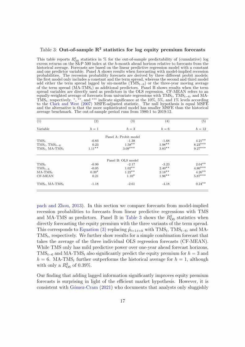
Table 3: Out-of-sample R2 statistics for log equity premium forecasts

This table reports R2OS statistics in % for the out-of-sample predictability of (cumulative) log

excess returns on the S&P 500 index at the h-month ahead horizon relative to forecasts from thehistorical average. Forecasts are based on the linear predictive regression model with a constantand one predictor variable. Panel A shows results when forecasting with model-implied recessionprobabilities. The recession probability forecasts are derived by three different probit models:the first model only includes a constant and the term spread, whereas the second and third modeladd either the term spread lagged by six-months (TMSt−6) or the three-year moving averageof the term spread (MA-TMSt) as additional predictors. Panel B shows results when the termspread variables are directly used as predictors in the OLS regression. CF-MEAN refers to anequally-weighted average of forecasts from univariate regressions with TMSt, TMSt−6, and MA-TMSt, respectively. ∗, ∗∗, and ∗∗∗ indicate significance at the 10%, 5%, and 1% levels accordingto the Clark and West (2007) MSFE-adjusted statistic. The null hypothesis is equal MSFEand the alternative is that the more sophisticated model has smaller MSFE than the historicalaverage benchmark. The out-of-sample period runs from 1980:1 to 2019:12.

(1) (2) (3) (4) (5)

Variable h = 1 h = 3 h = 6 h = 12

Panel A: Probit modelTMSt -0.83 -1.38 -1.68 4.21∗∗TMSt, TMSt−6 0.23 1.58∗∗ 1.98∗∗ 8.23∗∗∗TMSt, MA-TMSt 1.11∗∗ 3.09∗∗∗ 3.83∗∗ 9.27∗∗∗

Panel B: OLS modelTMSt -0.99 -2.17 -3.23 2.04∗∗TMSt−6 -0.05 1.02∗∗ 2.40∗∗ 4.80∗∗∗MA-TMSt 0.39∗ 1.22∗∗ 2.18∗∗ 4.26∗∗CF-MEAN 0.21 1.10∗ 1.96∗∗ 5.87∗∗∗

TMSt, MA-TMSt -1.18 -2.61 -4.18 0.24∗∗

pach and Zhou, 2013). In this section we compare forecasts from model-impliedrecession probabilities to forecasts from linear predictive regressions with TMSand MA-TMS as predictors. Panel B in Table 3 shows the R2

OS statistics whendirectly forecasting the equity premium with the three variants of the term spread.This corresponds to Equation (3) replacing pt+1:t+h with TMSt, TMSt−6, and MA-TMSt, respectively. We further show results for a simple combination forecast thattakes the average of the three individual OLS regression forecasts (CF-MEAN).While TMS only has mild predictive power over one-year ahead forecast horizons,TMSt−6 and MA-TMSt also significantly predict the equity premium for h = 3 andh = 6. MA-TMSt further outperforms the historical average for h = 1, althoughwith only a R2

OS of 0.39%.

Our finding that adding lagged information significantly improves equity premiumforecasts is surprising in light of the efficient market hypothesis. However, it isconsistent with Gomez-Cram (2021) who documents that analysts only sluggishly

17

revise their expectations downward and that stock prices do not fully reflect pub-licly available information on turning points. The last row in Panel B shows theperformance of a joint OLS regression with TMSt and MA-TMSt. The OLS regres-sion analogue to our probit model performs worst, in line with the common findingthat multivariate regression models with several parameters often underperformthe historical average. Importantly, at all forecast horizons even the best linearmodels are substantially outperformed by the equity premium forecasts based onrecession probabilities.

The upper panel of Figure 5 superimposes one-month ahead equity premium fore-casts from the recession probability based on TMSt and MA-TMSt (solid blackline), the analogue OLS model with the two predictors (dashed black line), andthe historical average benchmark (solid gray line). While the OLS model gener-ates forecasts that are volatile both in recessions and expansions, the probit modelforecasts are relatively stable in expansions and markedly higher than the histori-cal average. As the implied recession probabilities are high just before the 1981-82recession, the implied equity premium forecasts are sharply negative around thattime. This effect, although substantially less pronounced, is also visible aroundthe business cycle peaks in 2001 and 2007.

Welch and Goyal (2008) have popularized a simple way to visualize the relativeforecast performance of different prediction models over time. The lower panelin Figure 5 follows their approach and plots the difference in cumulative squaredforecast errors (CSFE) for the historical average and the CSFE for two differentmodels: the solid black line depicts equity premium forecasts based on the im-plied recession probability using TMS and MA-TMS, whereas the dashed blackline shows the OLS model with both TMS and MA-TMS. An increasing curveindicates superior performance relative to the naive benchmark. We can see thatthe curve for the OLS model is decreasing over most of the sample, with reversedtrends only around the 1981-82 and 2001 recessions. In contrast, the curve forthe probit model forecasts is rising over most of the sample, indicating that therecession probability forecast of the equity premium consistently outperforms thehistorical average.

This superior performance is driven by two distinct effects. First, and similar tothe OLS model, the model significantly predicts the negative excess returns in theone-year window around the peak in 1981. This is consistent with Table 1 andwith the notion that term spread information anticipates recessions. Second, andmore importantly, the model-implied recession probabilities outperform the naivebenchmark also in expansions. This contrasts the “no predictability in good timespuzzle” that is often documented in related articles (Huang, Jiang, Tu, and Zhou,2017). The explanation is simple: Table 1 shows that the annualized equity pre-

18

mium averages 6.31% in our sample, but is even higher at an annualized 8.40% inexpansions. While the historical average closely tracks the full-sample average, ourrecession probability-based forecast corrects for negative values around businesscycle peaks and thus correctly predicts a higher equity premium in expansions.

3.5 Structural break in the mean of the term spread

We have seen above that the implied recession probabilities are muted and rarelyexceed 50% after the mid-1980s. This is consistent with e.g. Chauvet and Potter(2002) who find evidence for a structural break in the probit model based on theterm spread but argue that the exact date of the break is difficult to localize. Whenfixing the break to 1984, they show that the model is able to predict the recessionin 2001 with probabilities as high as 90% for the 12 month ahead forecast hori-zon. Galvao (2006) proposes a structural break threshold-VAR (SBTVAR) modelthat allows for non-linearities and breaks in the link between the term spread andU.S. output growth and identifies a break in 1985:2. She further shows that theSBTVAR model correctly anticipates the 2001 recession in real-time. Other pa-pers also document breaks in the dynamic relationship between the term spreadand real growth. Chauvet and Potter (2010) find evidence for recurrent breaksin a probit model with industrial production, sales, personal income, and employ-ment. Schrimpf and Wang (2010) analyze whether the predictive power of the termspread on output growth suffers from structural breaks. They allow for multiplebreaks using the test procedure of Bai and Perron (1998, 2003) and find evidencefor breaks in Germany, Canada, U.K., and the U.S.

To summarize, there is ample prior evidence for a structural break in the linkbetween the term spread and output growth, as well as for a break in the esti-mated recession probabilities from the standard probit model. This suggests thataccounting for such a break may improve the recession probability forecasts andhence the equity premium predictability. In what follows, we provide further ev-idence for a structural break. Instead of focusing on a break in the estimatedrelation between the term spread and future recessions, we focus our attentionon a break in the mean of the term spread. Figure 2 plots the normalized termspread from 1951:3 to 2019:12. Eyeballing this time series shows that the mean ofthe term spread has shifted upwards in the early 1980s. This is most visible whencomparing the period from 1965 to 1982 with the period from 1983 to 2019: themean of the former period is -0.61 whereas it is 0.46 for the latter period. In whatfollows, we formally test the hypothesis of a structural break in the mean of theterm spread.

The classical break test for coefficients in linear regression models goes back to

19

1980 1990 2000 2010 2020

−2 %

−1 %

0 %

1 %

2 %

TMSt and MA−TMSt (probit model)TMSt and MA−TMSt (OLS model)Historical average

1980 1990 2000 2010 2020

−0.

010

−0.

005

0.00

00.

005

0.01

0

TMSt and MA−TMSt (probit model)TMSt and MA−TMSt (OLS model)

Figure 5: Out-of-sample forecasts and performance over timeThis figure shows one-month ahead forecasts of the log equity premium for three different models(upper panel). The solid black line depicts forecasts from model-implied recession probabilityforecasts of a probit model with the term spread (TMS) and the backward-looking three-yearmoving average of the term spread (MA-TMS). The dashed black line presents forecasts froma standard linear predictive regression model with TMS and MA-TMS as predictors, and thesolid gray line denotes the historical average. The lower panel shows the difference betweencumulative squared forecast errors (CSFE) of the historical average and the CSFE of the probitmodel forecasts (solid black line) and the OLS model forecasts (dashed black line). All forecastsare estimated with a recursively expanding information set that mimics the real-time situationof an investor. The out-of-sample period is 1980:1 to 2019:12.

20

Chow (1960). A critical limitation of the Chow-test is that the break date has tobe known a priori. Here, we treat the break date as unknown and perform breaktests over a grid of candidate values – namely on a fraction of the sample between[τ1, τ2] with τ1 = πτT and τ2 = (1 − πτ )T . We refer to πτ as the trimming value.When performing the Chow test on a sequence of dates the standard chi-squarecritical values are not applicable; for a discussion of this point see Hansen (2001).We estimate the following model for all z values between [τ1, τ2]:

TMSt = β1I{t ≤ z}+ β2I{t > z}+ εt, (5)

where I{t ≤ z} (I{t > z}) is an indicator function that equals one for t ≤ z(t > z). The coefficients β1 and β2 are re-estimated for a grid of z values and theSSE values are saved for each of these grid points. If there is no structural breakin the coefficients then the SSE values vary randomly over time. However, if thereis a unique structural break, then the time series will have a well-defined globalminimum near the true break date (Hansen, 2001).

The upper panel in Figure 6 presents the SSE as a function of z with a trimmingvalue of πτ = 0.15. The SSE is thus calculated for potential breaks from 1961:6to 2009:8. The resulting SSE clearly shows a strong v-shape, indicating a welldefined and unique break point. The break date corresponds to the month withthe lowest sum of squared errors (Bai, 1997). This global minimum is in 1982:5.We formally test the null hypothesis of no structural break by using the Sup-F,Ave-F, and Exp-F statistics of Andrews (1993) and Andrews and Ploberger (1994).The variance-covariance matrix is estimated according to Newey and West (1994)and the p-values are computed following Hansen (1997). The null hypothesisof no structural break is rejected at the 1% significance level for Sup-F, Ave-F,and Exp-F and is robust to changes in the trimming value and pre-whitening ofthe residuals; details are provided in the Online Appendix. The middle panel inFigure 6 presents the estimated sub-sample means in the term spread with fullsample information. The upward shift in the mean is consistent with attenuatedrecession probabilities after the break that we have observed above.

The previous test results are based on full sample information. Would an investorhave been able to identify the break in real-time? To answer this question weestimate the p-values with a recursively expanding sample from 1980:1 onwardsand re-estimate the p-values each month until 2019:12. The lower panel in Figure 6presents the resulting series of p-values. The null hypothesis of no structural breakis first rejected at the 10% critical value by the Sup-F, Ave-F, and Exp-F tests in1986:7, 1987:3, and 1986:9. Since then, the p-values have consistently remainedbelow 5%, providing strong evidence that the break in the mean of the term spreadcould have been identified in real-time as early as the mid 1980s. From 1995:1 to

21

2019:12 the null hypothesis is always rejected at the 1% level for each of the teststatistics. The estimated break date is identical for the different test statistics asit is simply localized at the global minimum of the sum of squared errors (Bai,1997).7 Overall, the results are in line with other evidence of structural breaks inthe standard probit model and the estimated break date is close to the structuralchange in variance of U.S. GDP growth in the early 1980s, see e.g. Kim and Nelson(1999), McConnell and Perez-Quiros (2000), and Pettenuzzo and Timmermann(2017).8

3.6 Forecasting in the presence of structural breaks

We have documented in the previous section that the term spread suffers from astructural break in the mean. We now show how to adjust forecasts in the presenceof such a break.

First, we apply the procedure by Lettau and Van Nieuwerburgh (2008). Theyfind evidence in favor of multiple shifts in the mean of the dividend-price ratio. Tocorrect for these breaks, they create a break-adjusted time series by subtracting thesub-sample means from the dividend-price ratio. They then show that the adjustedtime series has robust in-sample predictive power for the equity premium but failsto beat the historical average out-of-sample. Lettau and Van Nieuwerburgh (2008)argue that the break dates can be estimated in real-time but that the uncertaintyabout the shift in the mean prevents significant forecasting gains.9

7Figure A.3 in the Online Appendix displays recursively estimated break dates from 1980:1to 2019:12. This shows that the identified break dates are very stable around the full-samplebreak date 1982:5.

8We also test for multiple breaks in the mean of the term spread by applying the methodsproposed in Bai and Perron (1998, 2003). The sequential tests do not provide evidence in favor ofmultiple breaks. Moreover, we apply the sequential tests to a longer sample that starts in 1933:4,just after the Great Depression. Interestingly, we find evidence for another break in the meanin 1947:6, in addition to the one in 1982:5. The additional break aligns well with the Treasury-Federal Reserve Accord, indicating a change in monetary policy after longer-term interest rateswere pegged during wartime (Eichengreen and Garber, 1991; Carlson and Wheelock, 2014).

9Smith and Timmermann (2021) present a method that uses cross-sectional information andeconomically motivated priors to (i) better detect breaks in real-time and to (ii) estimate pa-rameters more accurately. The latter point is especially relevant when only few post-breakobservations are available.

22

1950 1960 1970 1980 1990 2000 2010 2020

0.12

0.13

0.14

0.15

1950 1960 1970 1980 1990 2000 2010 2020

−0.

020.

000.

020.

04

1950 1960 1970 1980 1990 2000 2010 2020

0.0

0.2

0.4

0.6

0.8

1.0

Sup−FAve−FExp−F

Figure 6: SSE as a function of the break date and real-time detection of the break

This figure presents the sum of squared errors (SSE) when testing for a structural beak in the mean of the termspread (upper panel). The change point is allowed to lie between 1961:6 and 2009:8, which corresponds to a trimmingvalue of 15%. The analysis is based on full sample information and the coefficients and SSE are re-estimated foreach potential break date. The middle panel shows the term spread from 1951:3 to 2019:12 (solid line) and thesub-sample means from 1951:3 to 1982:5 and from 1982:6 to 2019:12 (dashed line). The estimated break date isin 1982:5 and corresponds to the global minimum in SSE (Bai, 1997). The lower panel reports the recursivelyestimated p-values of the null hypothesis of no structural break (Hansen, 1997). This analysis is feasible in real-timeand recursively expands the information set. Sup-F, Ave-F, and Exp-F refer to the Wald-type statistics of Andrews(1993) and Andrews and Ploberger (1994). The dashed (dotted) horizontal line shows the 10% (5%) level. Theestimation of p-values is carried out from 1980:1 to 2019:12.

23

In our setting, we use monthly data and a trimming value of 15%. The samplestarts in 1951:3 and the first real-time detection of a break is in 1986:7. Specifically,we carry out the following steps: we first test for a break in the mean of the termspread by estimating the Sup-F statistic and using a significance level of 10%.Only real-time information is used to mimic the situation of an investor. Second,if the null hypothesis of no break is rejected, we estimate the two sub-sample meansand subtract them from the term spread to create a break-adjusted term spread,denoted by TMSbreak. Finally, we estimate the probit model with this adjustedtime series and generate out-of-sample forecasts for recession probabilities and thelog equity premium. If the null hypothesis is not rejected, we forecast with theunadjusted probit model.

Alternative approaches have been proposed by Pesaran and Timmermann (2007).They present methods to determine the optimal estimation window in the presenceof structural breaks. These methods are based on the insight that if the pre-breakdata follow a data generating process that is different from the one characterizingthe post-break data, then the coefficient estimates are biased when using all data.Pesaran and Timmermann (2007) show in a simulation study that the MSFE canbe significantly reduced by combining different forecasts from the same modelwhen a structural break is present. The individual forecasts only differ in theirestimation window. While some models mainly use post-break data, other modelsmake use of all available historical data. Specifically, one estimates the model overan equally-spaced grid of starting points between the start of the data set and theidentified break date and then combines the forecasts using simple averages.

We implement the combination of different forecasts from our probit models asfollows. First, we test for a structural break in the term spread by applying theSup-F test. If no break is identified, we forecast with the unadjusted probit model.Second, if the null hypothesis of no break is rejected, we estimate the probit modelover an equally-spaced grid of start values. This grid starts at the beginning ofour data set and continues until the estimated break date. To reduce computingtime, we only estimate models at annual increments in the starting date. Thisprovides us with multiple recession forecasts and equity premium forecasts thatonly differ in the start date of the estimation window. Third, our pooled forecast issimply the average of the individual forecasts over the grid of start values, denotedas ”Pooling (average)”. Additionally, we have estimated forecasts from weightedpooling. As the differences are negligible, we only show results for the equal-weighted combination of forecasts.10

10We demand at least 15 years of data in the probit model to guarantee reliable coefficientestimates. Suppose that the Sup-F test first identifies in 1986:7 that a break has occurred in1981:3. Then, the shortest estimation window uses data starting in 1969:7. This is because we

24

A disadvantage of the pooling approach is that one includes many forecasts witha large fraction of pre-break data when the sample is long or when the breakoccurs relatively late in the sample. Alternatively, one can only choose the bestperforming grid point. We implement this approach by performing a pseudo out-of-sample exercise over the most recent five years of data. We allow for the samegrid points as for pooling but with the extension that we lose the five most recentstart values because of this evaluation period. Then we evaluate all start valuesover this holdout period and select the start value that minimizes the MSFE forthe equity premium. The selection of the grid point is chosen based on forecastsof the log equity premium and not on forecasts of the probit model as the formeris the main purpose of this paper. Forecasts from this approach are denoted as”Cross-validation”.

Finally, we consider one estimation strategy that only uses post-break data toestimate parameters of the probit model and to forecast recession probabilitiesand the equity premium. We denote this strategy as ”Post-break window”.11 Ifthe null hypothesis of no structural break is not rejected, then the forecasts ofthe break-correction methods are identical to forecasts by the unadjusted probitmodel. In what follows, we apply these break-adjustment methods to the probitmodel with TMS and MA-TMS as predictors.

Figure 7 shows recession probability forecasts for cross-validation and for post-break window, as well as for the standard probit model with the term spread. Theestimated probabilities for cross-validation remain at fairly low levels during the1990-91 and 2001 recessions for short-horizon forecasts. However, the probabilitiesfor the 2008-09 recession increase substantially relative to the unadjusted full-sample models. They rise above 60% for cross-validation and are thus considerablyhigher than the probabilities in Figure 3 which are less than 30% for h = 1 andunadjusted models. Moreover, for h = 12 we see a substantially improved forecastperformance with estimated probabilities as high as 90% for the 2001 and 2008-09 recessions. Post-break window generates out-of-sample probabilities as high as90% for the 2001 recession, however, this approach also gives rise to a false positive

have to lag the data by 17 years (not 15 years) to account for the delay in NBER announcements.Hence, the probit model is estimated over the grid of start dates from 1969:7,1968:7,... until thestart of the sample. For MA-TMS we lose 35 observations and, therefore, do not start in 1951:3but in 1954:2. We always include the beginning of the sample in the grid of start values, even ifthe distance to the next grid point is less than one year. Results remain qualitatively the same forsix-month steps between start dates. Note that the estimation window of the linear predictiveregression model for the equity premium varies as well. For example, when the probabilityforecasts are derived only with data from 1970:1 onward, then the same holds true for the equitypremium forecasts.

11We use at least 15 years of data. Hence, while the sample of post-break data is shorter than15 years we use the most recent 15 years of data for estimation and forecasting.

25

in the late 1990s. Overall, we confirm previous findings that the implied recessionprobabilities are more pronounced when properly correcting for instabilities andbreaks (Galvao, 2006; Chauvet and Potter, 2010). We provide forecast evaluationstatistics for the break-correction methods in the Online Appendix.

3.7 Correcting for structural breaks: Out-of-sample equitypremium prediction

We have seen in the previous section that the recession probability forecastsare substantially higher in the second part of the sample when using the cross-validation and post-break window approaches to correct for the break in the meanof the term spread in 1982. In this section we compare the equity premium fore-casts from recession probabilities of the probit model with the unadjusted termspread and moving average term spread with forecasts from the same model whenapplying the break-correction methods. We will see that the break adjustmentsubstantially improves the equity premium predictability of the implied recessionprobabilities.

Table 4 provides the R2OS statistics for the out-of-sample equity premium predic-

tion using the break-correction methods to adjust the term spread relative to thehistorical average. Panel A shows that the one month ahead forecasts improvefor each of the four methods, and that the R2

OS is as high as 3.2% for post-breakwindow for the prediction sample from 1980:1 to 2019:12, shown in column (1).Columns (2) to (4) show theR2

OS values for different subsamples. While the gains instatistical predictability relative to the historical average are significant also from1980-1999 (column (2)), they are much stronger for the period since 2000 (column(3)). The R2

OS statistics in this sub-period exceed 3% for break-adjusted termspread, cross-validation, and post-break window. It is worth noting that the esti-mated predictive coefficients (not shown) are consistently negative and highlightthat the superior performance relative to the historical average is driven by nega-tive equity premium forecasts during recessions. This is in contrast with Campbelland Thompson (2008) who argue that imposing non-negativity constraints on theequity premium can improve performance.

The results are qualitatively the same for longer forecast horizons, shown in panelsB to D. The R2

OS statistics are consistently positive for the different sub-samplesand gradually increase in the forecast horizon h - with R2

OS values above 10% for cu-mulative one year ahead equity premiums. The only exception is the probit modelwith the break-adjusted term spread which has negative values between 1980:1to 1999:12, resulting from a poor performance during the 1990s. Comparing thedifferent break-adjustment methods of Pesaran and Timmermann (2007), we ob-

26

h = 1 h = 3

1980 1990 2000 2010 2020

0.0

0.2

0.4

0.6

0.8

1.0

TMSt

Cross−validationPost−break window

1980 1990 2000 2010 2020

0.0

0.2

0.4

0.6

0.8

1.0

TMSt


h = 6 h = 12

1980 1990 2000 2010 2020

0.0

0.2

0.4

0.6

0.8

1.0

TMSt


1980 1990 2000 2010 2020

0.0

0.2

0.4

0.6

0.8

1.0

TMSt


Figure 7: Out-of-sample performance: (break-corrected) recession prob-abilitiesThis figure presents out-of-sample recession probability forecasts for four different forecast hori-zons and three different models. The forecasts denote the probability of a recession within thenext h = 1, 3, 6, 12 months. The solid gray line shows forecasts from the standard probit modelwith the term spread as the only predictor (TMSt). The solid black line depicts forecasts from aprobit model with the term spread and the moving average component (MA-TMSt), where theoptimal estimation window is determined by cross-validation over a holdout period of 60 months.The dashed black line presents forecasts from a probit model with TMS and MA-TMS that onlyuses post-break data for coefficient estimation. Out-of-sample forecasts are recursively estimatedfor the sample from 1980:1 to 2019:12.

serve a clear pattern. The approach that only uses post-break data performs best,closely followed by cross-validation, and with some distance followed by pooling.In our setting, the break in the mean is relatively sizable and the break-date can be

27

Table 4: Out-of-sample R2 statistics when correcting for a structural break

This table presents R2OS statistics (in %) for forecasts of the h = 1, 3, 6, 12 months ahead (cumulative) log equity

premium. This statistic measures the reduction in MSFE relative to forecasts from the historical average.Results are shown for a probit model with the term spread and the moving average component as predictors,and for four methods that correct for a structural break in the mean of the term spread. The first methodforecasts with a break-adjusted term spread (TMSbreak

t , 136

∑35j=0TMSbreak

t−j ), see Lettau and Van Nieuwerburgh

(2008). Cross-validation selects an optimal estimation window over a holdout period, whereas pooling combinesforecasts from several models with a grid of different starting values. Post-break window refers to forecastsfrom a model that only uses post-break data. For further details see Section 3.6 and Pesaran and Timmermann(2007). Short interest and gold-to-platinum ratio are the predictors of Rapach et al. (2016) and Huang andKilic (2019), and perfect classifier refers to a simple two-state model that can perfectly anticipate NBER-datedrecessions. ∗, ∗∗, ∗∗∗ denote significance at the 10%, 5%, and 1% significance levels according to the Clark andWest (2007) MSFE-adjusted statistic. Columns (1) to (4) report results for different sub-samples, and panelsA to D present results for different forecasting horizons.

(1) (2) (3) (4)Variable 1980:1-2019:12 1980:1-1999:12 2000:1-2019:12 1990:1-2013:12Panel A: h = 1TMSt, MA-TMSt 1.11∗∗ 1.52∗∗ 0.67∗∗ 0.74∗∗

TMSbreakt , MA-TMSbreak

t 1.60∗∗∗ 0.03 3.29∗∗∗ 2.17∗∗Cross-validation 2.27∗∗∗ 1.30∗∗ 3.31∗∗ 2.94∗∗Pooling (average) 1.45∗∗∗ 1.33∗∗ 1.59∗∗∗ 1.40∗∗∗Post-break window 3.21∗∗∗ 1.64∗∗ 4.89∗∗∗ 4.57∗∗∗

Perfect classifier 1.06∗ 0.10 2.09∗ 1.74∗Short interest 1.67∗∗Gold-to-platinum ratio 1.15∗∗

Panel B: h = 3TMSt, MA-TMSt 3.09∗∗∗ 4.40∗∗ 1.84∗∗ 2.17∗∗


t 3.41∗∗∗ -1.11 7.80∗∗∗ 4.56∗∗Cross-validation 7.25∗∗∗ 3.70∗∗ 10.76∗∗ 9.25∗∗Pooling (average) 4.10∗∗∗ 3.95∗∗ 4.26∗∗∗ 3.78∗∗∗Post-break window 8.78∗∗∗ 4.43∗∗ 13.12∗∗∗ 11.69∗∗∗

Perfect classifier 2.50∗ 0.27 4.71∗ 3.74∗Short interest 5.46∗∗∗Gold-to-platinum ratio 4.54∗∗

Panel C: h = 6TMSt, MA-TMSt 3.83∗∗ 5.04∗∗ 2.91∗ 3.54∗∗


t 3.02∗∗ -7.34 10.94∗∗∗ 5.91∗∗Cross-validation 10.53∗∗∗ 3.16∗ 16.04∗∗ 14.25∗∗Pooling (average) 5.54∗∗∗ 4.10∗ 6.62∗∗∗ 6.01∗∗∗Post-break window 11.36∗∗∗ 5.45∗∗ 15.78∗∗ 15.49∗∗

Perfect classifier 3.63∗ -0.13 6.43∗ 5.49∗Short interest 9.44∗∗Gold-to-platinum ratio 8.52∗∗

Panel D: h = 12TMSt, MA-TMSt 9.27∗∗∗ 10.10∗∗ 8.87∗∗ 8.58∗∗∗


t 8.08∗∗ -8.75 18.74∗∗∗ 8.17∗Cross-validation 12.28∗∗∗ 7.76∗ 15.27∗∗∗ 14.13∗∗Pooling (average) 11.89∗∗∗ 7.73∗ 14.56∗∗∗ 11.38∗∗∗Post-break window 16.67∗∗∗ 13.22∗∗ 19.10∗∗ 18.45∗∗

Perfect classifier 10.23∗∗∗ 3.70∗ 14.52∗∗∗ 12.55∗∗Short interest 7.85∗Gold-to-platinum ratio 9.55∗∗

28

Table 5: Out-of-sample R2 statistics in recessions and expansions

This table presents R2OS statistics (in %) for forecasts of the h = 1, 3, 6, 12 months ahead (cumu-

lative) log equity premium. Results are shown for a probit model with the term spread (TMS)and the moving average component (MA-TMS) as predictors, and for four methods that correctfor a structural break in the steady state mean of the term spread. For further details see Section3.6. The R2

OS statistics are displayed separately for recessions and expansions. ∗, ∗∗, ∗∗∗ denotesignificance at the 10%, 5%, and 1% significance levels according to the Clark and West (2007)MSFE-adjusted statistic. Column (1) reports the respective forecasting model, and columns (2)to (5) present results for different forecasting horizons. The out-of-sample period is 1980:1 to2019:12.

(1) (2) (3) (4) (5)

Variable h = 1 h = 3 h = 6 h = 12

Panel A: RecessionsTMSt, MA-TMSt 1.83∗ 2.59∗ -1.08 -1.20TMSbreak

t , MA-TMSbreakt 5.94∗∗ 9.00∗∗ 5.95∗∗ 9.44∗∗

Cross-validation 6.72∗∗ 14.15∗∗ 15.11∗∗ 8.33∗∗∗Pooling (average) 3.40∗∗ 5.41∗∗ 2.74∗∗ 4.77∗∗∗Post-break window 9.84∗∗∗ 17.62∗∗∗ 18.20∗∗ 17.72∗∗

Panel B: ExpansionsTMSt, MA-TMSt 0.86∗∗ 3.35∗∗∗ 7.03∗∗ 15.31∗∗∗TMSbreak

t , MA-TMSbreakt 0.11 0.54∗∗ 1.11∗ 7.29∗∗

Cross-validation 0.75∗∗ 3.70∗∗∗ 7.56∗∗∗ 14.56∗∗∗Pooling (average) 0.79∗∗ 3.43∗∗∗ 7.37∗∗∗ 16.00∗∗∗Post-break window 0.93∗∗ 4.22∗∗∗ 6.91∗∗∗ 16.07∗∗∗

estimated accurately in real-time. Therefore, the improvements from pooling aresmallest, due to the large impact of pre-break information. Cross-validation seemsto be the most robust choice both for improving recession and equity premiumforecasts. The post-break window also works well in our application but may bemore risky from an ex ante perspective, putting all weight on post-break forecasts.Hence, our preferred break-correction method is cross-validation.12

To better understand the strong predictive power of recession probabilities for theequity premium, we provide separate R2

OS statistics for expansions and recessionsin Table 5. Strikingly, we see that for essentially all considered models and forecasthorizons, there is an economically and statistically significant improvement overthe historical average benchmark in both recessions and expansions. As discussedabove, the reason is the following. Recession probabilities correctly predict low eq-uity premiums in recessions. In addition, by adjusting for low equity premiums inrecessions they correctly predict higher equity premiums than the historical aver-

12We show the recursively selected estimation windows for one-year ahead forecasts from cross-validation in the Online Appendix.

29

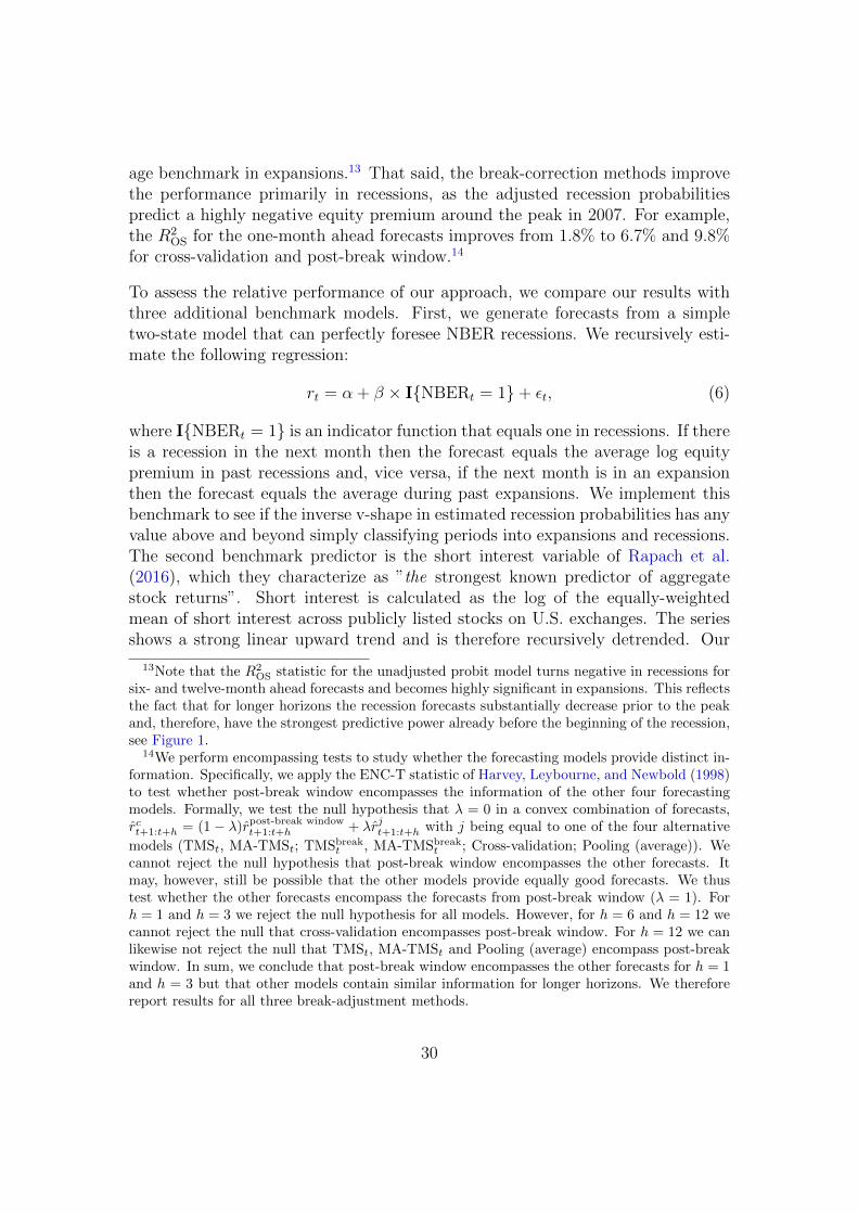
age benchmark in expansions.13 That said, the break-correction methods improvethe performance primarily in recessions, as the adjusted recession probabilitiespredict a highly negative equity premium around the peak in 2007. For example,the R2

OS for the one-month ahead forecasts improves from 1.8% to 6.7% and 9.8%for cross-validation and post-break window.14

To assess the relative performance of our approach, we compare our results withthree additional benchmark models. First, we generate forecasts from a simpletwo-state model that can perfectly foresee NBER recessions. We recursively esti-mate the following regression:

rt = α + β × I{NBERt = 1}+ εt, (6)

where I{NBERt = 1} is an indicator function that equals one in recessions. If thereis a recession in the next month then the forecast equals the average log equitypremium in past recessions and, vice versa, if the next month is in an expansionthen the forecast equals the average during past expansions. We implement thisbenchmark to see if the inverse v-shape in estimated recession probabilities has anyvalue above and beyond simply classifying periods into expansions and recessions.The second benchmark predictor is the short interest variable of Rapach et al.(2016), which they characterize as ”the strongest known predictor of aggregatestock returns”. Short interest is calculated as the log of the equally-weightedmean of short interest across publicly listed stocks on U.S. exchanges. The seriesshows a strong linear upward trend and is therefore recursively detrended. Our

13Note that the R2OS statistic for the unadjusted probit model turns negative in recessions for

six- and twelve-month ahead forecasts and becomes highly significant in expansions. This reflectsthe fact that for longer horizons the recession forecasts substantially decrease prior to the peakand, therefore, have the strongest predictive power already before the beginning of the recession,see Figure 1.

14We perform encompassing tests to study whether the forecasting models provide distinct in-formation. Specifically, we apply the ENC-T statistic of Harvey, Leybourne, and Newbold (1998)to test whether post-break window encompasses the information of the other four forecastingmodels. Formally, we test the null hypothesis that λ = 0 in a convex combination of forecasts,rct+1:t+h = (1− λ)rpost-break window

t+1:t+h + λrjt+1:t+h with j being equal to one of the four alternative

models (TMSt, MA-TMSt; TMSbreakt , MA-TMSbreak

t ; Cross-validation; Pooling (average)). Wecannot reject the null hypothesis that post-break window encompasses the other forecasts. Itmay, however, still be possible that the other models provide equally good forecasts. We thustest whether the other forecasts encompass the forecasts from post-break window (λ = 1). Forh = 1 and h = 3 we reject the null hypothesis for all models. However, for h = 6 and h = 12 wecannot reject the null that cross-validation encompasses post-break window. For h = 12 we canlikewise not reject the null that TMSt, MA-TMSt and Pooling (average) encompass post-breakwindow. In sum, we conclude that post-break window encompasses the other forecasts for h = 1and h = 3 but that other models contain similar information for longer horizons. We thereforereport results for all three break-adjustment methods.

30

third benchmark is the (log) gold-to-platinum ratio of Huang and Kilic (2019),constructed as the log of the ratio of gold to platinum prices, which the authorsshow to perform particularly well out-of-sample over longer forecast horizons.15

Due to data availability, we can only evaluate the latter two predictors over ashorter sample from 1990:1 to 2013:12.

We see in Column (4) of Table 4 that cross-validation and post-break windowconsistently outperform the three benchmark models for each forecast horizon.The gains in reduced MSFEs are substantial, with an R2

OS statistic that is oftentwice as large. The R2

OS of cross-validation is 2.94% for h = 1, compared to1.67% for short interest, 1.15% for gold-to-platinum ratio, and 1.74% for a perfectrecession classifier.16 At the one-year ahead horizon, cross-validation delivers anR2

OS statistic of more than 14%, compared to 7.85% for short interest and 9.55%for the gold-to-platinum ratio.

Figure 8 plots the difference in CSFE for the historical average and CSFE fordifferent models using recession probabilities: the unadjusted probit model, as wellas cross-validation, pooling, and post-break window. An increasing line indicatesthat the historical mean is outperformed during this period, whereas the oppositeis true for a decreasing line. The upper panel presents results for one month aheadforecasts. The solid gray line shows the relative performance for the unadjustedprobit model. It performs very well during the 1981-82 recession but does onlyincrease slightly compared to the other models thereafter. For cross-validation andpooling we see a similar pattern until 2007, which is followed by a positive jumpduring the Great Recession. The post-break window performs best, with a positivetrend since the mid 1990s, and the sharpest rise during the 2008-09 recession. Thechart thus shows that the predictability is strongest during recessions, but stillweakly present during some expansionary periods. This is consistent with previousevidence of time-varying predictive power (Rapach and Zhou, 2013; Jiang et al.,2019).

The lower panel depicts the performance for one year ahead forecasts. While thepicture is qualitatively the same as for the one month ahead forecasts, the basicmodel without break corrections shows a strong upward trend since 1995, which isnot exclusively driven by recessions. The model clearly outperforms the historicalaverage since 2009.17 Nonetheless, the break-correction approaches still perform

15We thank Dave Rapach for making the data publicly available on his homepage, and DarienHuang and Mete Kilic for kindly sharing their data with us.

16The results differ slightly compared to those published in the papers because our historicalaverage uses data from 1951:3 onwards. We re-estimate the predictive coefficients recursivelyusing expanding data available in real-time.

17The range of the vertical axis is smaller for h = 1 than for h = 12. This simply reflects that

31

better, and the ordering remains unchanged: the post-break window performsbest, followed by cross-validation and pooling. The distance between the lattertwo approaches substantially shrinks compared to the one month ahead forecasts.This can be explained by the observation that the unadjusted model performsbetter for h = 12 than for h = 1, and, as pooling includes many forecasts that aresimilar to this model, pooling also performs comparatively well.

Figure 9 compares the relative performance of cross-validation and post-breakwindow with the performance of short interest and gold-to-platinum ratio. Theupper (lower) panel shows results for one month (cumulative one year) aheadforecasts. None of the depicted models strongly outperforms the historical averagebetween 1990 and the onset of the Great Recession. Even though the gold-to-platinum ratio performs well from 2001 to 2003 the gains are offset between 2004to 2007. The models have in common that the positive R2

OS statistics are the resultof superior predictability between 2007 to 2013. The picture is similar for one-year ahead forecasts: the curves for short interest and gold-to-platinum ratio havenegative values prior to the 2008-09 crisis and strongly outperform the historicalaverage in the subsequent years. The CSFE curves for cross-validation and post-break window are solidly above the curves for the two benchmark predictors forboth horizons.

3.8 Implications for asset allocation

In this section we analyze the economic value of the improved equity premium pre-dictions. Cenesizoglu and Timmermann (2012) show that the correlation betweenstatistical and economic measures of forecast performance is positive but typicallyof low magnitude. Specifically, many models produce negative R2

OS values whilestill providing investors with improved Sharpe ratios and gains in the certaintyequivalent return. Interestingly, the reverse – positive R2

OS values and negativeeconomic gains – is observed less often. We follow Dangl and Halling (2012) andRapach et al. (2016) and others and consider a mean-variance investor who allo-cates funds across the equity market portfolio and the risk-free rate. At the endof period t, the investor optimally invests a share ωt in the risky asset:

ωt =1

γ

rt+1

σ2t+1

, (7)

averaging of 12 month ahead log equity premiums generates a substantially smoother time-series.This smoothed series can better be predicted, resulting in smaller squared forecast errors thanfor the one month ahead log equity premium.

32

1980 1990 2000 2010 2020

0.00

00.

005

0.01

00.

015

0.02

00.

025

0.03

0

TMSt and MA−TMSt

Cross−validationPooling (average)Post−break window

1980 1990 2000 2010 2020

0.00

00.

005

0.01

00.

015

TMSt and MA−TMSt

Cross−validationPooling (average)Post−break window

Figure 8: Out-of-sample performance over timeThis figure presents the difference between cumulative squared forecast errors (CSFE) of thehistorical average and the CSFE of four different forecasting models. The upper panel (lowerpanel) shows results for forecasts of the one month ahead (cumulative one year ahead) log equitypremium. Recession probabilities are derived by the probit model with TMS and MA-TMS(solid gray line), and for three methods that correct for a structural break in the term spread.These methods are cross-validation (solid black line), pooling (dotted black line), and post-breakwindow (dashed black line). The forecasting period is 1980:1 to 2019:12 and vertical bars denoterecessions.

33

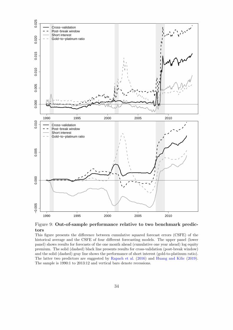
1990 1995 2000 2005 2010

0.00

00.

005

0.01

00.

015

0.02

00.

025

Cross−validationPost−break windowShort interestGold−to−platinum ratio

1990 1995 2000 2005 2010

−0.

005

0.00

00.

005

0.01

0

Cross−validationPost−break windowShort interestGold−to−platinum ratio

Figure 9: Out-of-sample performance relative to two benchmark predic-torsThis figure presents the difference between cumulative squared forecast errors (CSFE) of thehistorical average and the CSFE of four different forecasting models. The upper panel (lowerpanel) shows results for forecasts of the one month ahead (cumulative one year ahead) log equitypremium. The solid (dashed) black line presents results for cross-validation (post-break window)and the solid (dashed) gray line shows the performance of short interest (gold-to-platinum ratio).The latter two predictors are suggested by Rapach et al. (2016) and Huang and Kilic (2019).The sample is 1990:1 to 2013:12 and vertical bars denote recessions.

34

where γ is the coefficient of relative risk aversion and rt+1 is a forecast of theequity premium.18 Similar to Rapach et al. (2016), we estimate the variance ofexcess returns, σ2

t+1, as a 10-year rolling window of past data. Thus, ωt only differsbecause of the different equity premium forecasts implied by the various models,rt+1. The realized portfolio return, rPt+1, is:

rPt+1 = ωtrt+1 + rft+1, (8)

where rt+1 is the realized excess equity market return in period t + 1 and rft+1 isthe risk-free rate between period t and t+1. Furthermore, the certainty equivalentreturn (CER) can be calculated as:

CERP = µP −γ

2σ2P , (9)

where µP and σ2P are the sample mean and variance of the portfolio over the

out-of-sample period. We multiply the CER by 12 to interpret it as the annualrisk-free rate that an investor would be willing to accept to not hold the riskyportfolio (Chen et al., 2020). The difference in CER of two models – also knownas utility gain – can be interpreted as the annual portfolio management fee that aninvestor would be willing to pay to have access to the alternative forecasting model(Ferreira and Santa-Clara, 2011). Additionally, we calculate the annualized Sharperatio (SR) to evaluate the risk-return profile of the chosen portfolio allocations.

Table 6 presents ∆CER and ∆SR for monthly re-balancing for the sample periods1980-2019 (Panel A) and 1990-2013 (Panel B).19 The CER and SR values for theprevailing mean model are shown in the first row of each panel. All subsequentrows then provide differences of CER and SR with respect to that benchmark. Weimplement a bootstrap approach similar to DeMiguel, Plyakha, Uppal, and Vilkov(2013) to evaluate the statistical significance.20 We consider different specificationsfor the coefficient of relative risk aversion (γ) and for leverage and short-sellingconstraints (range of ω). Over the baseline sample period from 1980-2019, theprobit model with TMS and MA-TMS provides utility gains in the range of 1.4%to 2.7%. Hence, an investor would be willing to pay between 140 to 270 basispoints annually - depending on risk preferences and constraints - to have accessto the equity premium forecasts of this model. The gains are highest when γ isthree and when leveraging and short-selling up to 50% is allowed. Nonetheless,even an investor with ω between zero and one would be willing to pay a portfolio

18Forecasts in this section are based on excess returns rather than log excess returns.19We show in the Online Appendix that the results remain qualitatively the same when re-

balancing in 3-, 6-, 12-month intervals.20We set the average block length to three months (Politis and Romano, 1994).

35

management fee above 100 basis points annually. These gains further increasewhen correcting for the structural break in the mean of the term spread. Wesee a similar pattern as for the statistical predictability: the post-break windowperforms best, followed by cross-validation and the break-adjusted term spread,while gains for pooling are smallest. That said, any of these strategies outperformsa simple buy-and-hold strategy shown in the last row – often the gains more thantriple or quadruple. Similarly, the annualized Sharpe ratio rises from around 0.50for the historical average to between 0.65 to 0.85 for the break-correction methods.Panel B shows that the gains are comparable with and often substantially betterthan those for short interest and the gold-to-platinum ratio.

The upper panel in Figure 10 displays the optimal share in risky assets over time forthe post-break window and pooling approaches relative to the historical average;γ is set to three and ω is allowed to vary between -0.5 and 1.5. Naturally, equitypremium forecasts based on the historical average are continuously positive andchange only slowly, hence the weights are very persistent and always above 0.5.In contrast, the portfolio weights for pooling are most often above those for thehistorical average in expansions and below in recessions. This is most salient inthe early 1980s, where the share in risky assets runs down to -0.5 at the beginningof the recession and then quickly reverses to more than 1.0 toward the end ofthe recession. Similar patterns – even though less pronounced – are observed forthe 2001 and 2008-09 recessions. The post-break window signals for four of fiverecessions in the sample to short the equity market prior to the beginning of arecession when the yield curve has been flattening for some time and to moveback aggressively into the market towards the end of the recession when the yieldcurve is steepening again. Interestingly, both break-adjustment models signal torun down equity exposure at the end of our sample in 2019 due to rising recessionprobability forecasts.

The lower panel in Figure 10 shows the log cumulative wealth for five portfolioallocations: post-break window, cross-validation, pooling, historical average, andfor the buy-and-hold strategy. While the buy-and-hold and historical averageportfolios suffer severe losses in the Global Financial Crisis of 2008-2009, thisplunge is less pronounced for pooling and even reversed for post-break windowand cross-validation. Post-break window performs best, as it further signals to goshort prior to the 2001 recession. An investor that would have started with $1in 1979:12, reinvests all proceeds, and forecasts according to post-break window(cross-validation) would have earned $957 ($528) in 2019:12, compared to $90 forthe buy-and-hold strategy. Overall, the results in this section show that the break-correction methods outperform the naive benchmarks, and generate utility gainsthat are mostly superior to those of other recently proposed predictors.

36

Table 6: Asset allocation exercise

This table reports the annualized ∆CER and the annualized ∆SR for a mean-variance investor relativeto forecasts from the historical average. The investor can invest in the S&P 500 index and the risk-free rate. Results are shown for one month ahead forecasts of the equity premium and different valuesfor the coefficient of relative risk aversion (γ), and different restrictions on the equity weights (ω). The”Prevailing mean” shows the CER and SR values, whereas all other values denote the improvementsrelative to this benchmark. Panel A (Panel B) shows results for the out-of-sample period from 1980:1to 2019:12 (1990:1 to 2013:12). ∗, ∗∗, ∗∗∗ indicate significantly improved performance relative to theprevailing mean benchmark at the 10%, 5%, and 1% significance level. The p-values are obtained by usinga bootstrap approach similar to DeMiguel et al. (2013) with the average block length set to three months(Politis and Romano, 1994).

(1) (2) (3) (4) (5) (6) (7) (8)

Panel A: 1980:1 to 2019:12∆CER ∆SR

γ 3 5 3 3 3 5 3 3ω [−0.5, 1.5] [−0.5, 1.5] [0, 1.5] [0, 1] [−0.5, 1.5] [−0.5, 1.5] [0, 1.5] [0, 1]

Prevailing mean 8.30 6.59 8.30 8.69 0.49 0.48 0.49 0.53

Gains relative to prevailing mean:TMSt, MA-TMSt 2.73∗∗∗ 1.49∗∗ 2.41∗∗∗ 1.39∗∗∗ 0.15∗∗∗ 0.14∗∗ 0.13∗∗∗ 0.10∗∗∗


t 4.07∗∗ 2.62∗∗ 3.33∗∗ 1.91∗ 0.30∗∗ 0.31∗∗ 0.25∗∗ 0.23∗∗Cross-validation 4.18∗∗∗ 2.77∗∗ 3.39∗∗∗ 2.29∗∗∗ 0.23∗∗∗ 0.24∗∗∗ 0.19∗∗∗ 0.18∗∗∗Pooling (average) 3.44∗∗∗ 2.10∗∗∗ 3.13∗∗∗ 2.12∗∗∗ 0.20∗∗∗ 0.20∗∗∗ 0.18∗∗∗ 0.16∗∗∗Post-break window 6.02∗∗∗ 4.20∗∗∗ 4.83∗∗∗ 3.01∗∗∗ 0.35∗∗∗ 0.35∗∗∗ 0.28∗∗∗ 0.25∗∗∗

Buy-and-hold 0.84∗ 0.36 0.84∗ 0.45∗ 0.06∗∗∗ 0.07∗∗ 0.06∗ 0.02∗

Panel B: 1990:1 to 2013:12∆CER ∆SR

γ 3 5 3 3 3 5 3 3ω [−0.5, 1.5] [−0.5, 1.5] [0, 1.5] [0, 1] [−0.5, 1.5] [−0.5, 1.5] [0, 1.5] [0, 1]

Prevailing mean 5.80 4.61 5.80 6.56 0.41 0.39 0.41 0.45

Gains relative to prevailing mean:TMSt, MA-TMSt 2.05∗∗ 1.24∗∗ 2.05∗∗ 0.72∗∗ 0.12∗∗∗ 0.13∗∗∗ 0.12∗∗∗ 0.05∗∗


t 5.68∗∗ 3.71∗∗ 4.71∗∗ 2.68 0.45∗∗ 0.47∗∗ 0.38∗∗ 0.32∗∗Cross-validation 4.44∗∗ 3.29∗∗ 3.66∗∗ 2.23∗ 0.26∗∗ 0.29∗∗ 0.21∗∗ 0.17∗Pooling (average) 3.56∗∗∗ 2.16∗∗ 3.56∗∗∗ 2.04∗∗∗ 0.21∗∗∗ 0.21∗∗∗ 0.21∗∗∗ 0.15∗∗∗Post-break window 8.11∗∗∗ 5.69∗∗ 6.59∗∗∗ 3.89∗∗∗ 0.48∗∗∗ 0.49∗∗∗ 0.39∗∗∗ 0.32∗∗∗

Short interest 3.58∗ 2.40∗ 3.24∗∗ 1.71 0.22∗ 0.22∗ 0.20∗∗ 0.16Gold-to-platinum ratio 4.03∗ 2.93∗ 4.11∗∗ 2.67∗ 0.28∗ 0.31∗ 0.30∗∗ 0.27∗∗Buy-and-hold 1.23∗ 0.23 1.23∗ 0.48∗ 0.08∗∗ 0.09∗ 0.08∗∗ 0.03∗

37

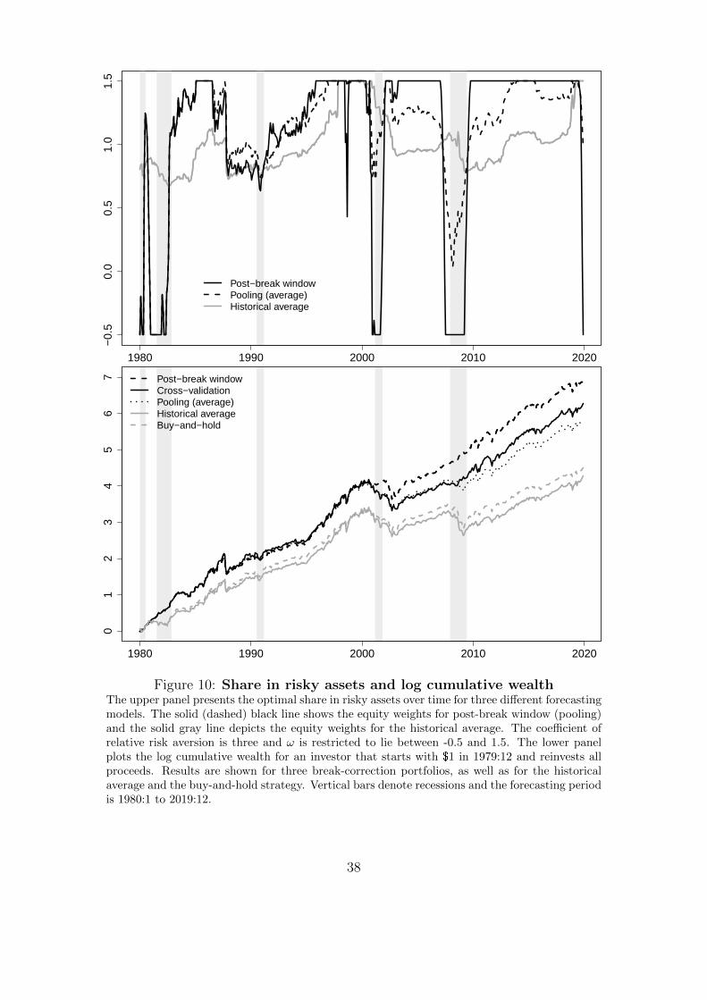
1980 1990 2000 2010 2020

−0.

50.

00.

51.

01.

5

Post−break windowPooling (average)Historical average

1980 1990 2000 2010 2020

01

23

45

67 Post−break window

Cross−validationPooling (average)Historical averageBuy−and−hold

Figure 10: Share in risky assets and log cumulative wealthThe upper panel presents the optimal share in risky assets over time for three different forecastingmodels. The solid (dashed) black line shows the equity weights for post-break window (pooling)and the solid gray line depicts the equity weights for the historical average. The coefficient ofrelative risk aversion is three and ω is restricted to lie between -0.5 and 1.5. The lower panelplots the log cumulative wealth for an investor that starts with $1 in 1979:12 and reinvests allproceeds. Results are shown for three break-correction portfolios, as well as for the historicalaverage and the buy-and-hold strategy. Vertical bars denote recessions and the forecasting periodis 1980:1 to 2019:12.

38

3.9 Forecasting characteristics portfolios

In this section, we extend our analysis to a rich set of equity portfolios. Specifi-cally, we follow Huang et al. (2015) and analyze the predictive power of recessionprobability forecasts for portfolios sorted on different characteristics. We focus on10 industry portfolios, 10 momentum portfolios, 10 size portfolios, and 10 book-to-market portfolios, all obtained from Kenneth French’s homepage.21 We predict thelog excess return for these portfolios with the same recession probability forecastsas in the previous sections. Results are shown in Table 7. We find that durable,manufacturing, energy, technology, and telecom portfolios are most predictable,whereas health, utility and nondurables are not significantly predictable. This isintuitive as the former sectors are more exposed to business cycle variation.22 In-terestingly, all of the momentum portfolios – independently of the break-correctionmethod – have positive and significant R2

OS statistics. Additionally, there is a ten-dency toward higher predictive power for portfolios formed on high market equity(large stocks) and low book-to-market ratios (growth stocks).

3.10 Dissecting the sources of predictability

In this section, we aim to shed light on the question whether the predictabilityof excess equity returns using recession probabilities derives from the cash flow orthe discount rate channel. To this end, we follow Campbell (1991) and Campbelland Ammer (1993) and apply a VAR decomposition to equity market returns.According to Campbell and Shiller (1988) the log return rt+1 can be rewritten as:

rt+1 = Et[rt+1] +NCFt+1 −NDR

t+1 , (10)

where Et[rt+1] is the conditional expectation of the log return at time t, and NCFt+1

and NDRt+1 represent cash flow and discount rate news, respectively. We use a

first-order VAR model to estimate the three components:

zt+1 = Γzt + ut+1. (11)

Here, zt is a k-dimensional vector of state variables, Γ is a k× k matrix of param-eters, and ut+1 is k-dimensional vector of innovations. We demean the variablesin the VAR model and, therefore, can omit an intercept. The cash flow news and

21The returns are value-weighted and include dividends.22It is also consistent with Da et al. (2017), who find that electricity usage better forecasts

excess returns of capital-intensive producers that are more exposed to fluctuations in the businesscycle and have higher operating leverage.

39

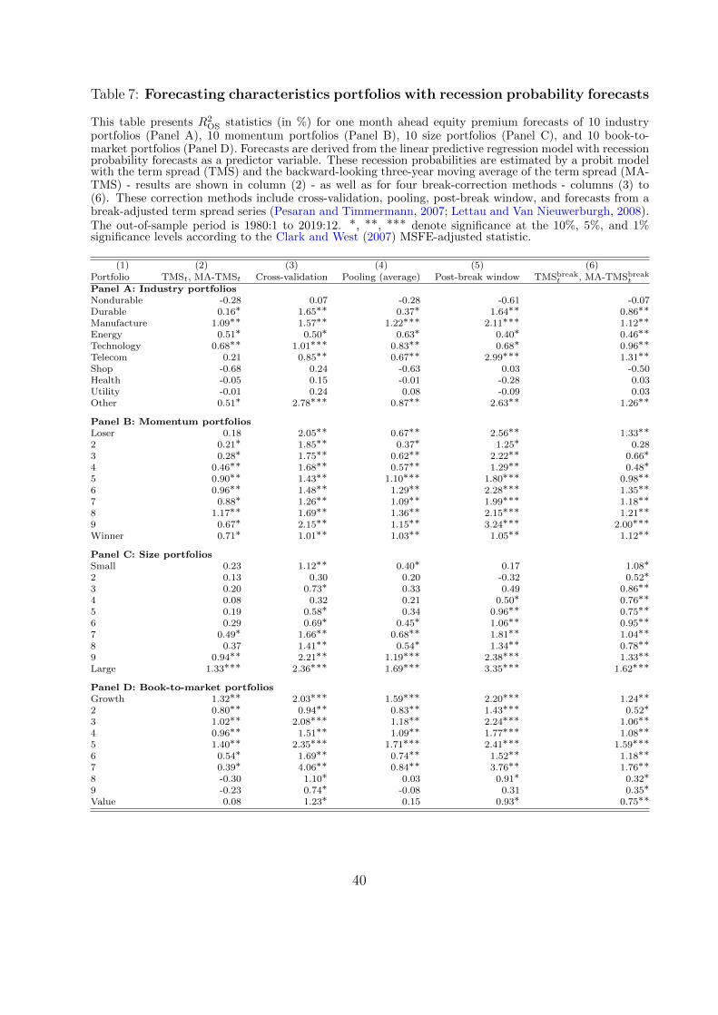
Table 7: Forecasting characteristics portfolios with recession probability forecasts

This table presents R2OS statistics (in %) for one month ahead equity premium forecasts of 10 industry

portfolios (Panel A), 10 momentum portfolios (Panel B), 10 size portfolios (Panel C), and 10 book-to-market portfolios (Panel D). Forecasts are derived from the linear predictive regression model with recessionprobability forecasts as a predictor variable. These recession probabilities are estimated by a probit modelwith the term spread (TMS) and the backward-looking three-year moving average of the term spread (MA-TMS) - results are shown in column (2) - as well as for four break-correction methods - columns (3) to(6). These correction methods include cross-validation, pooling, post-break window, and forecasts from abreak-adjusted term spread series (Pesaran and Timmermann, 2007; Lettau and Van Nieuwerburgh, 2008).The out-of-sample period is 1980:1 to 2019:12. ∗, ∗∗, ∗∗∗ denote significance at the 10%, 5%, and 1%significance levels according to the Clark and West (2007) MSFE-adjusted statistic.

(1) (2) (3) (4) (5) (6)Portfolio TMSt, MA-TMSt Cross-validation Pooling (average) Post-break window TMSbreak

t , MA-TMSbreakt

Panel A: Industry portfoliosNondurable -0.28 0.07 -0.28 -0.61 -0.07Durable 0.16∗ 1.65∗∗ 0.37∗ 1.64∗∗ 0.86∗∗Manufacture 1.09∗∗ 1.57∗∗ 1.22∗∗∗ 2.11∗∗∗ 1.12∗∗Energy 0.51∗ 0.50∗ 0.63∗ 0.40∗ 0.46∗∗Technology 0.68∗∗ 1.01∗∗∗ 0.83∗∗ 0.68∗ 0.96∗∗Telecom 0.21 0.85∗∗ 0.67∗∗ 2.99∗∗∗ 1.31∗∗Shop -0.68 0.24 -0.63 0.03 -0.50Health -0.05 0.15 -0.01 -0.28 0.03Utility -0.01 0.24 0.08 -0.09 0.03Other 0.51∗ 2.78∗∗∗ 0.87∗∗ 2.63∗∗ 1.26∗∗

Panel B: Momentum portfoliosLoser 0.18 2.05∗∗ 0.67∗∗ 2.56∗∗ 1.33∗∗2 0.21∗ 1.85∗∗ 0.37∗ 1.25∗ 0.283 0.28∗ 1.75∗∗ 0.62∗∗ 2.22∗∗ 0.66∗4 0.46∗∗ 1.68∗∗ 0.57∗∗ 1.29∗∗ 0.48∗5 0.90∗∗ 1.43∗∗ 1.10∗∗∗ 1.80∗∗∗ 0.98∗∗6 0.96∗∗ 1.48∗∗ 1.29∗∗ 2.28∗∗∗ 1.35∗∗7 0.88∗ 1.26∗∗ 1.09∗∗ 1.99∗∗∗ 1.18∗∗8 1.17∗∗ 1.69∗∗ 1.36∗∗ 2.15∗∗∗ 1.21∗∗9 0.67∗ 2.15∗∗ 1.15∗∗ 3.24∗∗∗ 2.00∗∗∗Winner 0.71∗ 1.01∗∗ 1.03∗∗ 1.05∗∗ 1.12∗∗

Panel C: Size portfoliosSmall 0.23 1.12∗∗ 0.40∗ 0.17 1.08∗2 0.13 0.30 0.20 -0.32 0.52∗3 0.20 0.73∗ 0.33 0.49 0.86∗∗4 0.08 0.32 0.21 0.50∗ 0.76∗∗5 0.19 0.58∗ 0.34 0.96∗∗ 0.75∗∗6 0.29 0.69∗ 0.45∗ 1.06∗∗ 0.95∗∗7 0.49∗ 1.66∗∗ 0.68∗∗ 1.81∗∗ 1.04∗∗8 0.37 1.41∗∗ 0.54∗ 1.34∗∗ 0.78∗∗9 0.94∗∗ 2.21∗∗ 1.19∗∗∗ 2.38∗∗∗ 1.33∗∗Large 1.33∗∗∗ 2.36∗∗∗ 1.69∗∗∗ 3.35∗∗∗ 1.62∗∗∗

Panel D: Book-to-market portfoliosGrowth 1.32∗∗ 2.03∗∗∗ 1.59∗∗∗ 2.20∗∗∗ 1.24∗∗2 0.80∗∗ 0.94∗∗ 0.83∗∗ 1.43∗∗∗ 0.52∗3 1.02∗∗ 2.08∗∗∗ 1.18∗∗ 2.24∗∗∗ 1.06∗∗4 0.96∗∗ 1.51∗∗ 1.09∗∗ 1.77∗∗∗ 1.08∗∗5 1.40∗∗ 2.35∗∗∗ 1.71∗∗∗ 2.41∗∗∗ 1.59∗∗∗6 0.54∗ 1.69∗∗ 0.74∗∗ 1.52∗∗ 1.18∗∗7 0.39∗ 4.06∗∗ 0.84∗∗ 3.76∗∗ 1.76∗∗8 -0.30 1.10∗ 0.03 0.91∗ 0.32∗9 -0.23 0.74∗ -0.08 0.31 0.35∗Value 0.08 1.23∗ 0.15 0.93∗ 0.75∗∗

40

discount rate news can be estimated as:

NCFt+1 = (e1′ + e1′λ)ut+1, (12)

NDRt+1 = e1′λut+1, (13)

where e1 is a k-vector with a one in the first cell and a zero in all remaining cells,and λ ≡ ρΓ(I − ρΓ)−1. We set ρ = 0.95

112 , which corresponds to approximately

5% consumption of total wealth per year (Campbell and Vuolteenaho, 2004; Maio,2013).

The state vector is assumed to capture the dynamics of log equity market re-turns. However, the estimated news components may be sensitive to the variablesincluded in the VAR (Chen and Zhao, 2009). Therefore, we follow Rapach et al.(2016) and estimate a series of trivariate VAR models including the log return se-ries, the dividend-price ratio, and one of the 14 commonly used Welch and Goyal(2008) predictors at a time.23 Additionally, we show results for a VAR model,where we add the first three principal components of the predictors of Welch andGoyal (2008) to the log return and the log dividend-price ratio (Rapach et al.,2016). We use the OLS estimates of Γ and ut+1 to calculate Et[rt+1], NCF

t+1 , and

NDRt+1 . Then, we run the following regressions to estimate the effect of our model-

implied recession probabilities on the components:

Et[rt+1] = αE + βE × pt+1 + εEt+1 (14)

NCFt+1 = αCF + βCF × pt+1 + εCFt+1 (15)

NDRt+1 = αDR + βDR × pt+1 + εDRt+1 (16)

While the return decomposition is based on the VAR estimates over the full samplefrom 1951:3 to 2019:12, we estimate the recession probabilities pt+1 with recursivelyexpanding information sets to rule out any look-ahead bias. Table 8 presents thecoefficients βE, βCF , and βDR estimated using data from 1980:1 to 2019:12 whichcorresponds to our out-of-sample forecasting period. As predictor we use the re-cession probabilities estimated by cross-validation, but the results are essentiallyunchanged for the alternative break-correction methods. The estimates show thatthe recession probability has significant predictive power for both the cash flowand the discount rate news component in most VAR specifications. Specifically,increased recession probabilities signal high expected returns but low future divi-

23The 14 predictors are the log dividend-price ratio (DP), log dividend yield (DY), log earnings-price ratio (EP), log dividend-payout ratio (DE), excess stock return volatility (RVOL), book-to-market ratio (BM), net equity expansion (NTIS), Treasury bill rate (TBL), long-term yield(LTY), long-term return (LTR), term spread (TMS), default yield spread (DFY), default returnspread (DFR), and inflation (INFL).

41

dends, consistent with the notion that in bad times investors expected high futurereturns and lower cash flows.

Our results are consistent with limited information processing of investors tomacroeconomic news. The term spread is readily available to investors and stockmarkets should be forward-looking. This implies that news about the business-cycle embedded in the term spread should be fully incorporated in stock prices.In contrast, our results show that recession probabilities using the term spreadas input provide valuable information to time the market. This is in line withstudies documenting information rigidities and sluggishness in forecast revisions.Rudebusch and Williams (2009) document that a simple probit model that isbased on the yield curve performs substantially better than professional forecast-ers in predicting recessions - even though evidence in favor of the former modelhas been known for years. Coibion and Gorodnichenko (2015) show for infla-tion forecasts of professional forecasters that the null hypothesis of consistencywith full-information rational expectations models can primarily be rejected dueto deviations from full-information. Their findings suggest that agents on averageupdate their information sets every six to seven months. An alternative interpre-tation of these results is that agents put a relatively small weight on incominginformation. Consistent with such a view, Loungani, Stekler, and Tamirisa (2013)find evidence of information rigidities in growth forecasts for a cross-section ofcountries, with an average period of 4 to 6 months until new information is fullyincorporated.

Information rigidities are not restricted to professional forecasters, however. Bouchaud,Kruger, Landier, and Thesmar (2019) document that analysts who are less experi-enced and follow more industries have stickier beliefs - consistent with informationprocessing constraints (Peng, 2005). Several articles show at the firm level thateven though information is publicly available, it is often not fully incorporated intostock prices, resulting in delayed price reaction to news (see, e.g., Bernard andThomas (1989); Huberman and Regev (2001); Hirshleifer, Lim, and Teoh (2009)).Chen et al. (2020) find that aggregate investor attention - extracted from 12 differ-ent attention measures - has predictive power for the aggregate stock market thatcannot be explained by macroeconomic fundamentals. Moreover, Gomez-Cram(2021) shows that news about impending recessions are incorporated into stockprices only with some delay. Analysts’ earnings forecasts are too optimistic whenthe excess return forecast is negative.

42

Table 8: Predictive regressions for stock market return components

This table presents slope coefficients for regressions of log stock market return components onmodel-implied recession probabilities. The stock market return is decomposed into the condi-tional return expectation (Et[rt+1]), a cash flow news component (NCF

t+1), and a discount rate

news component (NDRt+1 ). The decomposition is based on the VAR approach of Campbell (1991)

and Campbell and Ammer (1993) and includes as states the variables in columns (1) and (5).The log return on the S&P 500 index (r) and the log dividend-price ratio (DP) are included ineach of the VAR models. PC denotes the first three principal components of the 14 popularpredictors of Welch and Goyal (2008). The three return components are separately regressed ona constant and model-implied recession probabilities from cross-validation. The probabilities arerecursively estimated and identical to those used in the out-of-sample exercises in the previoussections. The regressions are based on data from 1980:1 to 2019:12. The t-statistics for the slopecoefficients are shown in the brackets below and the standard errors are HAC-robust (Andrews,1991). ∗, ∗∗, ∗∗∗ denote significance at the 10%, 5%, and 1% significance levels.

(1) (2) (3) (4) (5) (6) (7) (8)

VAR variables βE βCF βDR VAR variables βE βCF βDR

r, DP 0.04 -0.17∗∗ 0.30∗∗∗ r, DP, LTY 0.00 -0.17∗∗ 0.26∗∗[0.65] [-2.50] [2.76] [0.10] [-2.59] [2.36]

r, DP, DY 0.03 -0.17∗∗ 0.29∗∗∗ r, DP, LTR 0.06∗ -0.18∗∗∗ 0.32∗∗∗[0.58] [-2.49] [2.68] [1.77] [-2.62] [2.79]

r, DP, EP 0.04 -0.76∗∗ -0.29 r, DP, TMS -0.04 -0.15∗∗ 0.24∗∗[0.60] [-2.02] [-1.16] [-0.85] [-2.16] [2.10]

r, DP, DE 0.04 -0.76∗∗ -0.29 r, DP, DFY 0.07 -0.22∗∗∗ 0.28∗∗∗[0.60] [-2.02] [-1.16] [1.09] [-2.68] [2.73]

r, DP, RVOL 0.08 -0.20∗∗ 0.31∗∗∗ r, DP, DFR 0.03 -0.17∗∗ 0.30∗∗∗[1.14] [-2.55] [3.02] [0.53] [-2.49] [2.71]

r, DP, BM -0.01 -0.19∗∗ 0.23∗∗ r, DP, INFL -0.00 -0.17∗∗ 0.26∗∗[-0.27] [-2.54] [2.05] [-0.03] [-2.51] [2.07]

r, DP, NTIS 0.07 -0.15 0.35∗∗∗ r, DP, PC -0.00 -0.30∗∗∗ 0.13[1.61] [-1.49] [2.77] [-0.05] [-3.09] [1.17]

r, DP, TBL -0.06∗ -0.14∗ 0.24∗∗[-1.86] [-1.95] [2.00]

4 Robustness

In this section we show the robustness of our results along several dimensions. Theresults are provided in the Online Appendix.

First, we document that model-implied recession probabilities predict the eq-uity premium in four major economies: Germany, France, Canada, and the UnitedKingdom. Figure A.1 displays a similar v-shaped pattern of the cumulative one-year ahead log equity premium (

∑11j=0 rt+j) for the four countries around the begin-

ning of recessions. Hence, the result that equity premiums are negative headinginto recessions and then sharply recover is a universal phenomenon and not re-stricted to the U.S. We then generate out-of-sample recession probability forecastsand equity premium forecasts as explained in Sections 3.1 and 3.3 for these four

43

countries. We compare the performance of the three models with the same pre-dictors: (1) TMSt, (2) TMSt and TMSt−6, (3) TMSt and MA-TMSt. Details andresults are provided in Online Appendix B. We find positive significant R2

OS statis-tics for Germany, France and Canada for most of the different model specificationsand forecast horizons, whereas the R2

OS statistics for the UK are positive mainlyfor longer forecast horizons. Thus, our main finding that recession probabilitiespredict the equity premium extends to other major economies.24

Second, we provide R2OS statistics for different averaging windows to construct

MA-TMS and show that the results are robust to the exact choice of moving aver-age. In the main text we have focused on a moving average of three years for theUS. The long-horizon forecasts for h = 3, 6, 12 are statistically significant also formoving averages between one to five years, whereas the one-month ahead forecastsperform best for averages between three to five years.

Third, we present out-of-sample R2OS values for log raw returns (without sub-

tracting the short rate). The previous results carry over to raw returns, however,the predictive power decreases slightly for cumulative six- and twelve-month aheadforecasts.

Finally, we provide the certainty equivalent returns and Sharpe ratios whencorrecting for proportional transaction costs of 50 basis points per transaction(Balduzzi and Lynch, 1999). The gains relative to the historical average and thebuy-and-hold strategy remain sizable.

5 Conclusion

Excess equity market returns are negative around business cycle peaks, and stronglyrecover during recessions. In this paper, we have shown that probit models whichpredict recessions using the term spread also have strong predictive power forthe U.S. equity premium. The gains are statistically and economically significantand further improve when adding a backward-looking moving average of the termspread to the probit model. Equity premium forecasts based on recession prob-abilities correctly anticipate negative market returns heading into recessions andpositive returns in expansions. We provide evidence for a structural break in themean of the term spread in 1982. When correcting for this structural break, bothrecession and equity premium forecasts further improve. Our paper thus provides

24That said, there are some differences across countries with respect to the best-performingmodel for predicting recessions and the equity premium. The R2

OS statistics for models (2) and(3), which performed well for the US, are on average not better than those for model (1). Theincorporation of lagged term spread information does not have a positive effect on the recessionprobability forecasts in these countries and, therefore, also does not enhance the equity premiumforecasts. It is beyond the scope of this paper but would be interesting to analyze in futurewhether leading indicators other than the term spread further improve the results.

44

further evidence for the strong link between the business cycle and the equity pre-mium. More specifically, it shows that information in the yield curve can be usedto time the equity market.

References

Adrian, T., A. Estrella, and H. S. Shin (2019). Risk-taking channel of monetarypolicy. Financial Management 48, 725–738.

Andreasen, M. M., T. Engsted, S. V. Møller, and M. Sander (2020). The yieldspread and bond return predictability in expansions and recessions. Review ofFinancial Studies , 1–40.

Andrews, D. W. K. (1991). Heteroskedasticity and autocorrelation consistent co-variance matrix estimation. Econometrica 59 (3), 817–858.

Andrews, D. W. K. (1993). Tests for parameter instability and structural changewith unknown change point. Econometrica 61, 821–856.

Andrews, D. W. K. and W. Ploberger (1994). Optimal tests when a nuisanceparameter is present only under the alternative. Econometrica 62, 1383–1414.

Bai, J. (1997). Estimation of a change point in multiple regression models. Reviewof Economics and Statistics 79, 551–563.

Bai, J. and P. Perron (1998). Estimating and testing linear models with multiplestructural changes. Econometrica 66 (1), 47–78.

Bai, J. and P. Perron (2003). Computation and analysis of multiple structuralchange models. Journal of Applied Econometrics 18 (1), 1–22.

Balduzzi, P. and A. W. Lynch (1999). Transaction costs and predictability: someutility cost calculations. Journal of Financial Economics 52, 47–78.

Berge, T. J. and O. Jorda (2011). Evaluating the classification of economic ac-tivity into recessions and expansions. American Economic Journal: Macroeco-nomics 3 (2), 246–277.

Bernard, H. and S. Gerlach (1998). Does the term structure predict recessions?the international evidence. International Journal of Finance and Economics 3,195–215.

Bernard, V. L. and J. K. Thomas (1989). Post-earnings-announcement drift: De-layed price response or risk premium? Journal of Accounting Research 27,1–36.

45

Bouallegue, Z. B., L. Magnusson, T. Haiden, and D. S. Richardson (2019). Moni-toring trends in ensemble forecast performance focusing on surface variables andhigh-impact events. Quarterly Journal of the Royal Meteorological Society 145,1741–1755.

Bouchaud, J.-P., P. Kruger, A. Landier, and D. Thesmar (2019). Sticky expecta-tions and the profitability anomaly. Journal of Finance 74 (2), 639–674.

Campbell, J. Y. (1991). A variance decomposition for stock returns. EconomicJournal 101, 157–179.

Campbell, J. Y. and J. Ammer (1993). What moves the stock and bond market?a variance decomposition for long-term asset returns. Journal of Finance 48,3–37.

Campbell, J. Y. and R. J. Shiller (1988). The dividend-price ratio and expectationsof future dividends and discount factors. Review of Financial Studies 1 (3), 195–228.

Campbell, J. Y. and S. Thompson (2008). Predicting the equity premium outof sample: Can anything beat the historical average? Review of FinancialStudies 21, 1509–1531.

Campbell, J. Y. and T. Vuolteenaho (2004). Bad beta, good beta. AmericanEconomic Review 94 (5), 1249–1275.

Campbell, S. D. and F. X. Diebold (2009). Stock returns and expected businessconditions: Half a century of direct evidence. Journal of Business and EconomicStatistics 27, 266–278.

Carlson, M. A. and D. C. Wheelock (2014). Navigating constraints: The evolutionof federal reserve monetary policy, 1935-1959. Federal Reserve Bank of St. Louis,Working Papers 2014-13.

Cenesizoglu, T. and A. Timmermann (2012). Do return prediction models addeconomic value? Journal of Banking & Finance 36, 2974–2987.

Chauvet, M. and S. Potter (2002). Predicting a recession: evidence from the yieldcurve in the presence of structural breaks. Economics Letters 77, 245–253.

Chauvet, M. and S. Potter (2010). Business cycle monitoring with structuralchanges. International Journal of Forecasting 26, 777–793.

Chen, J., G. Tang, J. Yao, and G. Zhou (2020). Investor attention and stockreturns. Available at SSRN: https://papers.ssrn.com/sol3/papers.cfm?

abstract_id=3194387.

46

https://papers.ssrn.com/sol3/papers.cfm?abstract_id=3194387


Chen, L. and X. Zhao (2009). Return decomposition. Review of Financial Stud-ies 22 (12), 5213–5249.

Chen, S.-S., Y.-H. Chou, and C.-Y. Yen (2016). Predicting us recessions with stockmarket illiquidity. B.E. Journal of Macroeconomics 16, 93–123.

Chow, G. C. (1960). Tests of equality between sets of coefficients in two linearregressions. Econometrica 28, 591–605.

Christiansen, C., J. N. Eriksen, and S. V. Møller (2014). Forecasting us recessions:The role of sentiment. Journal of Banking and Finance 49, 459–468.

Clark, T. E. and K. D. West (2007). Approximately normal tests for equal pre-dictive accuracy in nested models. Journal of Econometrics 138, 291–311.

Cochrane, J. H. (2007). Financial markets and the real economy. In R. Mehra(Ed.), Handbook of the Equity Risk Premium, Chapter 7, pp. 237–325. Elsevier.

Coibion, O. and Y. Gorodnichenko (2015). Information rigidity and the expecta-tions formation process: A simple framework and new facts. American EconomicReview 105 (8), 2644–2678.

Cooper, I. and R. Priestley (2009). Time-varying risk premiums and the outputgap. Review of Financial Studies 22, 2801–2833.

Da, Z., D. Huang, and H. Yun (2017). Industrial electricity usage and stockreturns. Journal of Financial and Quantitative Analysis 52 (1), 37–69.

Dangl, T. and M. Halling (2012). Predictive regressions with time-varying coeffi-cients. Journal of Financial Economics 106, 157–181.

DeMiguel, V., Y. Plyakha, R. Uppal, and G. Vilkov (2013). Improving portfolioselection using option-implied volatility and skewness. Journal of Financial andQuantitative Analysis 48 (6), 1813–1845.

Diebold, F. X. and R. S. Mariano (1995). Comparing predictive accuracy. Journalof Business and Economic Statistics 13, 253–263.

Diebold, F. X. and G. D. Rudebusch (1989). Scoring the leading indicators. Journalof Business 62, 369–391.

Eichengreen, B. and P. Garber (1991). Before the accord: U.s. monetary-financialpolicy, 1945-1951. In Financial Markets and Financial Crises, pp. 175–206.National Bureau of Economic Research, Inc.

47

Estrella, A. (1998). A new measure of fit for equations with dichotomous dependentvariables. Journal of Business and Economic Statistics 16, 198–205.

Estrella, A. (2005, July). Why does the yield curve predict output and inflation?Economic Journal , 722–744.

Estrella, A. and G. A. Hardouvelis (1991). The term structure as a predictor ofreal economic activity. Journal of Finance 46, 555–576.

Estrella, A. and F. S. Mishkin (1998). Predicting u.s. recessions: financial variablesas leading indicators. Review of Economics and Statistics 80 (1), 45–61.

Estrella, A., A. P. Rodrigues, and S. Schich (2003). How stable is the predictivepower of the yield curve? evidence from germany and the united states. Reviewof Economics and Statistics 85, 629–644.

Fama, E. F. and K. R. French (1988). Dividend yields and expected stock returns.Journal of Financial Economics 22, 3–25.

Fama, E. F. and K. R. French (1989). Business conditions and expected returnson stocks and bonds. Journal of Financial Economics 25 (1), 23–49.

Ferreira, M. A. and P. Santa-Clara (2011). Forecasting stock market returns: Thesum of the parts is more than the whole. Journal of Financial Economics 100,514–537.

Ferson, W. E. and C. R. Harvey (1991). The variation of economic risk premiums.Journal of Political Economy 99, 385–415.

Fornaro, P. (2016). Forecasting us recessions with a large set of predictors. Journalof Forecasting 35, 477–492.

Galvao, A. B. (2006). Structural break threshold vars for predicting us recessionsusing the spread. Journal of Applied Econometrics 21, 463–487.

Galvao, A. B. and M. T. Owyang (2020). Forecasting low frequency macroeco-nomic events with high frequency data. FRB St. Louis Working Paper No.2020-028.

Gomez-Cram, R. (2021). Late to recessions: Stocks and the business cycle.Available at SSRN: https://papers.ssrn.com/sol3/papers.cfm?abstract_id=3671346.

Gu, S., B. Kelly, and D. Xiu (2020). Empirical asset pricing via machine learning.Review of Financial Studies 33, 2223–2273.

48



Hamilton, J. D. (2011). Calling recessions in real time. International Journal ofForecasting 27, 1006–1026.

Hanley, J. A. and B. J. McNeil (1982). The meaning and use of the area under areceiver operating characteristic (roc) curve. Radiology 143, 29–36.

Hanley, J. A. and B. J. McNeil (1983). A method of comparing the areas underreceiver operating characteristic curves derived from the same cases. Radiol-ogy 148, 839–843.

Hansen, B. E. (1997). Approximate asymptotic p-values for structural changetests. Journal of Business and Economic Statistics 15, 60–67.

Hansen, B. E. (2001). The new econometrics of structural change: Dating breaksin u.s. labor productivity. Journal of Economic Perspectives 15 (4), 117–128.

Harvey, D. I., S. J. Leybourne, and P. Newbold (1998). Tests for forecast encom-passing. Journal of Business and Economic Statistics 16, 254–259.

Hirshleifer, D., S. S. Lim, and S. H. Teoh (2009). Driven to distraction: Extraneousevents and underreaction to earnings news. Journal of Finance 64 (5), 2289–2325.

Huang, D., F. Jiang, J. Tu, and G. Zhou (2015). Investor sentiment aligned: Apowerful predictor of stock returns. Review of Financial Studies 28 (3), 791–837.

Huang, D., F. Jiang, J. Tu, and G. Zhou (2017). Forecasting stock returns ingood and bad times: The role of market states. Available at SSRN: https://papers.ssrn.com/sol3/papers.cfm?abstract_id=2188989.

Huang, D. and M. Kilic (2019). Gold, platinum, and expected stock returns.Journal of Financial Economics 132, 50–75.

Huberman, G. and T. Regev (2001). Contagious speculation and a cure for cancer:A nonevent that made stock prices soar. Journal of Finance 56 (1), 387–396.

Ibbotson, R. G. and R. A. Sinquefield (1976). Stocks, bonds, bills, and inflation:Year-by-year historical returns (1926-1974). Journal of Business 49, 11–47.

Jacobsen, B., B. R. Marshall, and N. Visaltanachoti (2019). Stock market pre-dictability and industrial metal returns. Management Science 65, 2947–3448.

Jiang, F., J. Lee, X. Martin, and G. Zhou (2019). Manager sentiment and stockreturns. Journal of Financial Economics 132, 126–149.

49



Johansson, P. (2018). Predicting recession probabilities using the slope of the yieldcurve. FEDS Notes. Washington: Board of Governors of the Federal ReserveSystem, March 1.

Kauppi, H. and P. Saikkonen (2008). Predicting u.s. recessions with dynamicbinary response models. Review of Economics and Statistics 90 (4), 777–791.

Kim, C.-J. and C. R. Nelson (1999). Has the u.s. economy become more stable?a bayesian approach based on a markov-switching model of the business cycle.Review of Economics and Statistics 81, 608–616.

Lacker, J. M. (2001). Introduction to special issue on the 50th anniversary of thetreasury-federal reserve accord. Federal Reserve Bank of Richmond EconomicQuarterly, Vol. 87.

Lettau, M. and S. Ludvigson (2001). Consumption, aggregate wealth, and expectedstock returns. Journal of Finance 56, 815–849.

Lettau, M. and S. Van Nieuwerburgh (2008). Reconciling the return predictabilityevidence. Review of Financial Studies 21 (4), 1607–1652.

Liu, W. and E. Moench (2016). What predicts us recessions? International Journalof Forecasting 32, 1138–1150.

Loungani, P., H. Stekler, and N. Tamirisa (2013). Information rigidity in growthforecasts: Some cross-country evidence. International Journal of Forecasting 29,605–621.

Lustig, H. and A. Verdelhan (2012). Business cycle variation in the risk-returntrade-off. Journal of Monetary Economics 58, 535–549.

Maio, P. (2013). Return decomposition and the intertemporal capm. Journal ofBanking and Finance 37, 4958–4972.

McConnell, M. M. and G. Perez-Quiros (2000). Output fluctuations in the unitedstates: What has changed since the early 1980’s? American Economic Re-view 90, 1464–1476.

Mihai, M. M. (2020). Do credit booms predict us recessions? Journal of Forecast-ing 39, 887–910.

Neely, C. J., D. E. Rapach, J. Tu, and G. Zhou (2014). Forecasting the equityrisk premium: The role of technical indicators. Management Science 60 (7),1772–1791.

50

Newey, W. K. and K. D. West (1987). A simple, positive semi-definite, het-eroskedasticity and autocorrelation consistent covariance matrix. Economet-rica 55 (3), 703–708.

Newey, W. K. and K. D. West (1994). Automatic lag selection in covariance matrixestimation. Review of Economic Studies 61, 631–653.

Nyberg, H. (2013). Predicting bear and bull stock markets with dynamic binarytime series models. Journal of Banking and Finance 37, 3351–3363.

Peng, L. (2005). Learning with information capacity constraints. Journal of Fi-nancial and Quantitative Analysis 40 (2), 307–329.

Pesaran, M. H. and A. Timmermann (2007). Selection of estimation window inthe presence of breaks. Journal of Econometrics (137), 134–161.

Pettenuzzo, D. and A. Timmermann (2017). Forecasting macroeconomic variablesunder model instability. Journal of Business and Economic Statistics 35, 183–201.

Pettenuzzo, D., A. Timmermann, and R. Valkanov (2014). Forecasting stock re-turns under economic constraints. Journal of Financial Economics 114, 517–553.

Politis, D. N. and J. P. Romano (1994). The stationary bootstrap. Journal of theAmerican Statistical Association 89 (428), 1303–1313.

Ponka, H. (2017). The role of credit in predicting us recessions. Journal of Fore-casting 36, 469–482.

Pyun, S. (2019). Variance risk in aggregate stock returns and time-varying returnpredictability. Journal of Financial Economics 132, 150–174.

Rapach, D. E., M. C. Ringgenberg, and G. Zhou (2016). Short interest and aggre-gate stock returns. Journal of Financial Economics 121, 46–65.

Rapach, D. E., J. K. Strauss, and G. Zhou (2010). Out-of-sample equity premiumprediction: Combination forecasts and links to the real economy. Review ofFinancial Studies 23 (2), 821–862.

Rapach, D. E., J. K. Strauss, and G. Zhou (2013). International stock returnpredictability: What is the role of the united states? Journal of Finance 68 (4),1633–1662.

Rapach, D. E. and G. Zhou (2013). Forecasting stock returns. In G. Elliott andA. Timmermann (Eds.), Handbook of Economic Forecasting, Volume 2A, pp.329–383. Elsevier, Amsterdam.

51

Rudebusch, G. D., B. P. Sack, and E. T. Swanson (2007). Macroeconomic im-plications of changes in the term premium. Federal Reserve Bank of St. LouisReview.

Rudebusch, G. D. and J. C. Williams (2009). Forecasting recessions: The puzzleof the enduring power of the yield curve. Journal of Business and EconomicStatistics 27, 492–503.

Schrimpf, A. and Q. Wang (2010). A reappraisal of the leading indicator prop-erties of the yield curve under structural instability. International Journal ofForecasting 26, 836–857.

Smith, S. C. and A. Timmermann (2021). Break risk. Review of Financial Stud-ies 34, 2045–2100.

Welch, I. and A. Goyal (2008). A comprehensive look at the empirical performanceof equity premium prediction. Review of Financial Studies 21, 1455–1508.

Wheelock, D. C. and M. E. Wohar (2009). Can the term spread predict outputgrowth and recessions? a survey of the literature. Federal Reserve Bank of St.Louis Review, September/October, Part 1.

Wright, J. H. (2006). The yield curve and predicting recessions. FEDS WorkingPaper No. 2006-7.

52

Online Appendix for“Equity premium predictability over the business cycle”

53

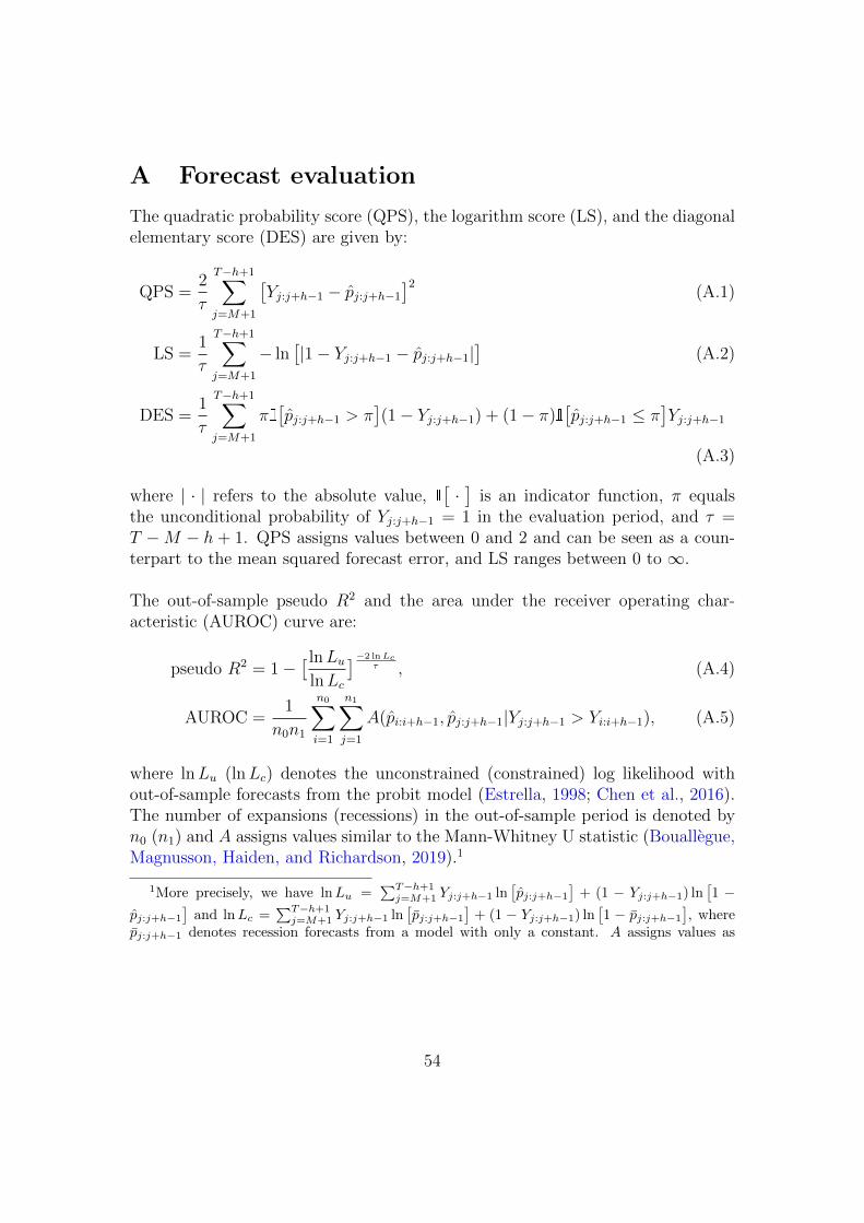
A Forecast evaluation

The quadratic probability score (QPS), the logarithm score (LS), and the diagonalelementary score (DES) are given by:

QPS =2

τ

T−h+1∑j=M+1

[Yj:j+h−1 − pj:j+h−1

]2(A.1)

LS =1

τ

T−h+1∑j=M+1

− ln[|1− Yj:j+h−1 − pj:j+h−1|

](A.2)

DES =1

τ

T−h+1∑j=M+1

πI[pj:j+h−1 > π

](1− Yj:j+h−1) + (1− π)I

[pj:j+h−1 ≤ π

]Yj:j+h−1

(A.3)

where | · | refers to the absolute value, I[·]

is an indicator function, π equalsthe unconditional probability of Yj:j+h−1 = 1 in the evaluation period, and τ =T −M − h + 1. QPS assigns values between 0 and 2 and can be seen as a coun-terpart to the mean squared forecast error, and LS ranges between 0 to ∞.

The out-of-sample pseudo R2 and the area under the receiver operating char-acteristic (AUROC) curve are:

pseudo R2 = 1−[ lnLu

lnLc

]−2 lnLcτ , (A.4)

AUROC =1

n0n1

n0∑i=1

n1∑j=1

A(pi:i+h−1, pj:j+h−1|Yj:j+h−1 > Yi:i+h−1), (A.5)

where lnLu (lnLc) denotes the unconstrained (constrained) log likelihood without-of-sample forecasts from the probit model (Estrella, 1998; Chen et al., 2016).The number of expansions (recessions) in the out-of-sample period is denoted byn0 (n1) and A assigns values similar to the Mann-Whitney U statistic (Bouallegue,Magnusson, Haiden, and Richardson, 2019).1

1More precisely, we have lnLu =∑T−h+1

j=M+1 Yj:j+h−1 ln[pj:j+h−1

]+ (1 − Yj:j+h−1) ln

[1 −

pj:j+h−1

]and lnLc =

∑T−h+1j=M+1 Yj:j+h−1 ln

[pj:j+h−1

]+ (1 − Yj:j+h−1) ln

[1 − pj:j+h−1

], where

pj:j+h−1 denotes recession forecasts from a model with only a constant. A assigns values as

54

B International evidence: Germany, France,

Canada, United Kingdom

In this appendix, we provide results on equity premium predictability using reces-sion probabilities for four additional countries: Germany, France, Canada, and theU.K. We download data for long-term interest rates and short-term interest ratesfrom the OECD.2 The long-term interest rates are for ten-year government bonds,the short-term interest rates are “based on three-month money market rates whereavailable”. Data are available from 1970:1 to 2019:12.3 The term spread is thedifference between the long-term and short-term interest rates. Recession data arefrom the Economic Cycle Research Institute. We download end-of-month data forthe DAX 30, CAC 40, S&P/TSX Composite index, and the FTSE 100 from Ya-hoo Finance and calculate monthly log excess return series. The data for Canadaare available from 1979:7 onward, while the series for Germany, France and theU.K. start in 1988:1, 1990:4, and 1984:1, respectively. We create a sample for thelog equity premium from 1980 onward by combining these series with data fromRapach, Strauss, and Zhou (2013) who provide equity premia for several devel-oped countries starting in 1980. The correlation of overlapping return data fromYahoo Finance and Rapach et al. (2013) is above 0.98 for Germany, France andthe U.K. We can thus splice both data sets to extend the sample back until 1980.The overlapping data have minor differences in their means; we correct for thisby adjusting the series to the mean of Rapach et al. (2013). The results with andwithout this mean correction are essentially identical.

Figure A.1 shows the behavior of the cumulative one-year ahead log equity pre-mium (

∑11j=0 rt+j) for the four countries around recessions. We see a clear v-shape

pattern similar to the one for the US. The solid gray lines depict the individual re-cessions, which show pronounced variation both in terms of magnitude and timing.Next, we perform a pseudo out-of-sample exercise for forecasting the log equitypremium from 1990:1 to 2019:12. In line with the U.S. example in the main text

follows:

A(pi:i+h−1, pj:j+h−1|Yj:j+h−1 > Yi:i+h−1) =

0 if pj:j+h−1 < pi:i+h−1, Yj:j+h−1 > Yi:i+h−1,

0.5 if pj:j+h−1 = pi:i+h−1, Yj:j+h−1 > Yi:i+h−1,

1 if pj:j+h−1 > pi:i+h−1, Yj:j+h−1 > Yi:i+h−1.

2https://data.oecd.org/interest/long-term-interest-rates.htm3The data for the UK short-term interest rate are downloaded from FRED. We use

the three month Treasury yield series until 2017:6 (https://fred.stlouisfed.org/series/IR3TTS01GBM156N) and the LIBOR (https://fred.stlouisfed.org/series/USD3MTD156N)from 2017:7 to 2019:12 (corrected for a minor difference in sample means).

55

https://data.oecd.org/interest/long-term-interest-rates.htm

https://fred.stlouisfed.org/series/IR3TTS01GBM156N

https://fred.stlouisfed.org/series/IR3TTS01GBM156N

https://fred.stlouisfed.org/series/USD3MTD156N

we compare the performance of three models: (1) TMSt, (2) TMSt and TMSt−6,(3) TMSt and MA-TMSt. Table A.1 shows the R2

OS statistics for the log equitypremium forecasts relative to a country-specific historical average. The values forGermany, France, and Canada are always positive and statistically significant foralmost all horizons when forecasting with the recession probabilities derived fromthe probit model with only the term spread. The R2

OS statistics for the U.K. arepositive only for h = 6 and h = 12. In contrast to the U.S., we do not see sig-nificant improvements by adding lagged and averaged term spread information tothe probit model. The reason is that the recession probabilities for models (2) and(3) do not predict the beginning of recessions better than the simple model (1).Overall, however, the international data provide additional support for the mainfinding that recession probabilities derived from the term spread help to time theequity market.

C Different lengths for moving average

Figure A.2 presents R2OS statistics (in %) for forecasts of the log equity premium.

The predictor variable is the recession probability forecast from a probit modelwith TMSt and 1

l

∑l−1j=0TMSt−j. We let the length of the moving average compo-

nent, denoted by l, vary between values of 2 and 60. The panels on the left ofFigure A.2 present the R2

OS values for h = 1, 6, 12 and the panels on the right de-pict the Clark and West (2007) statistics. The vertical axis denotes the R2

OS valuesand the MSFE-adjusted statistics and the horizontal axis denotes different valuesof l. We can see for h = 1 that the R2

OS is above 0.50% for any backward-lookingmoving average between 30 to 60 months and that the MSFE-adjusted statistic issignificant at the 5% level for these values. A shorter moving average of one yearalso has a R2

OS above 0.50% and is significant at the 10%. The R2OS for one-month

ahead forecasts is highest for moving averages between three to five years. Forcumulative six- and twelve-month ahead forecasts the R2

OS is always positive formoving averages between 2 to 60 months. A moving average between one to fiveyears has statistically significant R2

OS values above 2.50% (6%) for the six-month(twelve-month) horizon.

Table A.2 presents results for the break-correction methods when using valuesof l = 12, 24, 48, 60. The picture is similar to Figure A.2: the longer moving aver-ages perform better for short horizon forecasts, whereas the exact choice of movingaverage is less important for long horizon forecasts. The R2

OS values are positivefor all break-correction methods and moving averages. Furthermore, the resultsare robust to weighted pooling (Pooling (weighted)) and to a minimum windowlength of 20 years for post-break window (Post-break window (20 years)).

56

D Forecasting log raw returns

Table A.3 presents the R2OS statistics when forecasting the log raw returns instead

of the log equity premium (without subtracting the short rate). The results showthat recession probabilities have strong predictive power for equity market returnsnot only in excess of the risk-free rate.

E Transaction costs

Table A.4 shows the gains in certainty equivalent return and Sharpe ratio relativeto the prevailing mean when correcting for proportional transaction costs of 50basis points per transaction. This is similar to the base case in Balduzzi and Lynch(1999), which assumes proportional costs rather than fixed costs per transaction.This specification has often been used in related articles to account for tradingcosts; see, for example, Neely et al. (2014); Jiang et al. (2019). The results showthat even when proportional trading costs are taken into account, asset allocationbased on equity premium forecasts using recession probabilities provides investorswith an economically and statistically significant advantage relative to forecastsbased on the historical average.

F Asset allocation exercise for lower frequency

re-balancing

Table A.5 shows the gains in certainty equivalent return and Sharpe ratio whenan investor only re-balances the portfolio at the same frequency as the forecasthorizons of h = 3, 6, 12 months. Hence, non-overlapping forecasts are used in thisexercise; see Rapach et al. (2016) for details.

G Forecast evaluation: probit model with break-

corrections and alternative lengths of the mov-

ing average

Table A.6 presents the forecast evaluation statistics for the probit model with TMStand 1

36

∑35j=0TMSt−j as predictors, and for five break-corrected versions of this

model. We can see that the break-adjusted model (TMSbreakt , 1

36

∑35j=0TMSbreak

t−j )does not improve the forecast performance. Contrarily, for h = 1 the other meth-ods - cross-validation, pooling, and post-break window - have smaller (or identical)

57

values for QPS, LS, and DES. We have seen in the main text that post-break win-dow with at least 15 years of data in the probit model generates a false positiveprior to 2000. This is canceled out when setting the minimum number of obser-vations to 20 years. Thus, post-break window with 20 years performs even betterfor h = 1, 3, 6, 12 compared to post-break window with 15 years. Overall, cross-validation is most reliable in improving the performance relative to the unadjustedmodel; the statistics improve for each forecast horizon and each forecast evaluationstatistic.

Table A.7 presents the forecast evaluation statistics for the probit model withTMSt and 1

l

∑l−1j=0TMSt−j for values of l = 12, 24, 36, 48, 60. The statistics often

improve further for l = 12 and l = 24 compared to l = 36 but worsen for l = 48and l = 60. Nonetheless, the latter two values still provide superior values com-pared to the probit model without the moving average component. This is mostsalient for short-horizon forecasts and AUROC values.

H Recursively estimated break dates and opti-

mal starting points for cross-validation

The Sup-F, Ave-F, and Exp-F statistics are estimated as:

Sup-F = supτ1≤τ≤τ2

FT (τ), (A.6)

Ave-F =1

τ2 − τ1 + 1

τ2∑τ=τ1

FT (τ), (A.7)

Exp-F = ln[ 1

τ2 − τ1 + 1

τ2∑τ=τ1

expFT (τ)], (A.8)

where FT (τ) refers to the Wald statistic for testing β2 = β1 and τ = τ1, . . . , τ2.

The recursively estimated break dates for the Sup-F test are shown in the upperpanel of Figure A.3. The estimated location of the break is consistently between1981 and 1983.

The lower panel of Figure A.3 presents the selected start values from cross-validationfor one-year ahead log equity premium forecasts. At each point in time we estimatethe probit model with different estimation windows, and evaluate forecasts fromthese models over a pseudo out-of-sample period consisting of the most recent fiveyears of data. The optimal start value refers to the probit model with the smallest

58

MSFE for the cumulative log equity premium with h = 12. It is important tomention that this analysis is feasible in real-time without any look-ahead bias inthe data. Our most recently available observation at time t and h = 12 is rt−11:t.The evaluation period runs from rt−70:t−59, . . . , rt−11:t.

I Break tests with pre-whitening of standard er-

rors

Table A.8 provides p-values for the Ave-F, Exp-F, and Sup-F statistics when ap-plying pre-whitening to the standard errors. The null of no structural break isrejected for no pre-whitening, as well as for AR(1), AR(3), AR(6), and AR(12)pre-whitening. Furthermore, the results are robust to the choice of trimming value.

59

Germany (h = 12) France (h = 12)

−20 −10 0 10 20

−80 %

−60 %

−40 %

−20 %

0 %

20 %

40 %

Mean

−20 −10 0 10 20

−60 %

−40 %

−20 %

0 %

20 %

40 %

Mean

Canada (h = 12) United Kingdom (h = 12)

−20 −10 0 10 20

−60 %

−40 %

−20 %

0 %

20 %

40 %

Mean

−20 −10 0 10 20

−40 %

−20 %

0 %

20 %

Mean

Figure A.1: Log equity premium around business cycle peaks - Interna-tional evidenceThis figure presents the arithmetic average (solid black line) of the cumulative one-year aheadlog equity premium around the recessions in the sample from 1980:2 to 2019:12. The solid graylines depict the cumulative log equity premium of the individual recessions. The equity premiumis the difference between the country-specific end-of-month index return and the country-specificshort-term interest rate. The vertical axis depicts

∑11j=0 rt+j for t = −24, . . . ,−1, 0, 1, . . . , 24,

whereby rt+j is the log equity premium in month t+j. The horizontal axis displays the 24 monthsbefore and after a business cycle peak - with t = 0 referring to the first month of a recession.Recession indicators are taken from the Economic Cycle Research Institute and results are shownfor Germany, France, Canada, and the U.K.

60

Table A.1: Out-of-sample performance: Germany, France, Canada,United Kingdom

This table reports R2OS statistics in % for the out-of-sample predictability of (cumulative) log

excess returns at the h-month ahead horizon relative to forecasts from the historical average.Results are shown for Germany, France, Canada, and the U.K. Forecasts are based on thelinear predictive regression model with a constant and model-implied recession probabilities asa predictor variable. The recession probability forecasts are derived by three different probitmodels: the first model only includes a constant and the term spread, whereas the secondand third model add either the term spread lagged by six-months (TMSt−6) or the three-yearmoving average of the term spread (MA-TMSt) as additional predictors. ∗, ∗∗, and ∗∗∗ indicatesignificance at the 10%, 5%, and 1% levels according to the Clark and West (2007) MSFE-adjusted statistic. The null hypothesis is equal MSFE and the alternative is that the moresophisticated model has smaller MSFE than the historical average benchmark. The out-of-sample period is 1990:1 to 2019:12.

Variables in probit model h=1 h=3 h=6 h=12

Germany:TMSt 0.74∗∗ 1.93∗∗ 3.57∗ 7.35∗∗TMSt, TMSt−6 0.48 1.64∗ 3.57∗ 7.90∗∗TMSt, MA-TMSt 0.54∗ 1.44∗ 2.84∗ 7.77∗∗

France:TMSt 0.16 2.25∗∗ 3.90∗∗ 6.41∗∗∗TMSt, TMSt−6 0.53∗ 1.07∗∗ 3.46∗∗ 5.69∗∗∗TMSt, MA-TMSt 0.10 1.44∗∗ 2.75∗∗ -2.49

Canada:TMSt 2.32∗∗∗ 4.66∗∗∗ 8.53∗∗∗ 15.47∗∗∗TMSt, TMSt−6 2.24∗∗∗ 4.87∗∗∗ 7.45∗∗∗ 11.28∗∗∗TMSt, MA-TMSt -0.43 0.25 3.22∗∗ 7.22∗∗

United Kingdom:TMSt -0.44 -0.05 0.32 4.11∗∗TMSt, TMSt−6 0.19 2.12∗∗ 2.92∗∗ 5.45∗∗∗TMSt, MA-TMSt -0.10 0.10∗ 0.08∗ 0.57

61

R2OS (h = 1) MSFE-adjusted (h = 1)

0 10 20 30 40 50 60

−0.

20.

20.

61.

0

0 10 20 30 40 50 60

0.0

1.0

2.0

3.0


0 10 20 30 40 50 60

12

34

0 10 20 30 40 50 60

0.0

1.0

2.0

3.0


0 10 20 30 40 50 60

67

89

0 10 20 30 40 50 60

0.0

1.0

2.0

3.0

Figure A.2: Equity premium forecasts with different values of l in the probit modelThis figure presents R2

OS values (in %) for the log equity premium relative to the historical average and MSFE-adjusted

statistics. Forecasts are based on recession probability forecasts from a probit model with TMSt and 1l

∑l−1j=0TMSt−j ,

for l values between 2 and 60 months. The horizontal axis denotes the value of l and the vertical axis denotes the R2OS

statistic (left panels) and the MSFE-adjusted statistic of Clark and West (2007) (right panels). Results are shown forout-of-sample forecasts from 1980:1 to 2019:12 and for three forecast horizons, namely h = 1, 6, 12. The black dashedline (dotted line) denotes the 1% (5%) critical value, and the dash-dotted line depicts the 10% critical value of theMSFE-adjusted statistic.

62

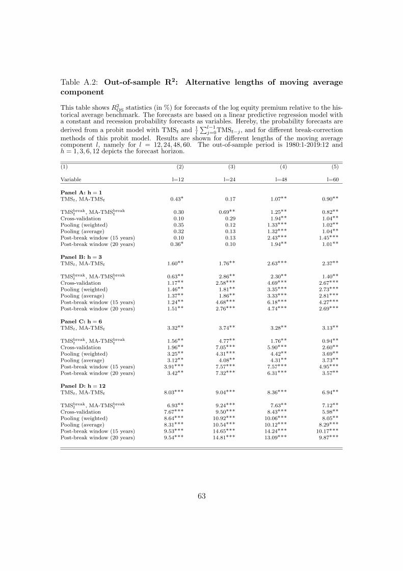
Table A.2: Out-of-sample R2: Alternative lengths of moving averagecomponent

This table shows R2OS statistics (in %) for forecasts of the log equity premium relative to the his-

torical average benchmark. The forecasts are based on a linear predictive regression model witha constant and recession probability forecasts as variables. Hereby, the probability forecasts are

derived from a probit model with TMSt and 1l

∑l−1j=0TMSt−j , and for different break-correction

methods of this probit model. Results are shown for different lengths of the moving averagecomponent l, namely for l = 12, 24, 48, 60. The out-of-sample period is 1980:1-2019:12 andh = 1, 3, 6, 12 depicts the forecast horizon.

(1) (2) (3) (4) (5)

Variable l=12 l=24 l=48 l=60

Panel A: h = 1TMSt, MA-TMSt 0.43∗ 0.17 1.07∗∗ 0.90∗∗


t 0.30 0.69∗∗ 1.25∗∗ 0.82∗∗Cross-validation 0.10 0.29 1.94∗∗ 1.04∗∗Pooling (weighted) 0.35 0.12 1.33∗∗∗ 1.02∗∗Pooling (average) 0.32 0.13 1.32∗∗∗ 1.04∗∗Post-break window (15 years) 0.10 0.13 2.43∗∗∗ 1.45∗∗∗Post-break window (20 years) 0.36∗ 0.10 1.94∗∗ 1.01∗∗

Panel B: h = 3TMSt, MA-TMSt 1.60∗∗ 1.76∗∗ 2.63∗∗∗ 2.37∗∗


t 0.63∗∗ 2.86∗∗ 2.30∗∗ 1.40∗∗Cross-validation 1.17∗∗ 2.58∗∗∗ 4.69∗∗∗ 2.67∗∗∗Pooling (weighted) 1.46∗∗ 1.81∗∗ 3.35∗∗∗ 2.73∗∗∗Pooling (average) 1.37∗∗ 1.86∗∗ 3.33∗∗∗ 2.81∗∗∗Post-break window (15 years) 1.24∗∗ 4.68∗∗∗ 6.18∗∗∗ 4.27∗∗∗Post-break window (20 years) 1.51∗∗ 2.76∗∗∗ 4.74∗∗∗ 2.69∗∗∗

Panel C: h = 6TMSt, MA-TMSt 3.32∗∗ 3.74∗∗ 3.28∗∗ 3.13∗∗


t 1.56∗∗ 4.77∗∗ 1.76∗∗ 0.94∗∗Cross-validation 1.96∗∗ 7.05∗∗∗ 5.90∗∗∗ 2.60∗∗Pooling (weighted) 3.25∗∗ 4.31∗∗∗ 4.42∗∗ 3.69∗∗Pooling (average) 3.12∗∗ 4.08∗∗ 4.31∗∗ 3.73∗∗Post-break window (15 years) 3.91∗∗∗ 7.57∗∗∗ 7.57∗∗∗ 4.95∗∗∗Post-break window (20 years) 3.42∗∗ 7.32∗∗∗ 6.31∗∗∗ 3.57∗∗

Panel D: h = 12TMSt, MA-TMSt 8.03∗∗∗ 9.04∗∗∗ 8.36∗∗∗ 6.94∗∗


t 6.93∗∗ 9.24∗∗∗ 7.63∗∗ 7.12∗∗Cross-validation 7.67∗∗∗ 9.50∗∗∗ 8.43∗∗∗ 5.98∗∗Pooling (weighted) 8.64∗∗∗ 10.92∗∗∗ 10.06∗∗∗ 8.05∗∗Pooling (average) 8.31∗∗∗ 10.54∗∗∗ 10.12∗∗∗ 8.29∗∗∗Post-break window (15 years) 9.53∗∗∗ 14.65∗∗∗ 14.24∗∗∗ 10.17∗∗∗Post-break window (20 years) 9.54∗∗∗ 14.81∗∗∗ 13.09∗∗∗ 9.87∗∗∗

63

Table A.3: Out-of-sample R2 statistics for log raw returns

This table presents R2OS statistics (in %) for forecasts of log raw returns relative to the historical

average benchmark. In contrast to the main text, we do not subtract the short rate from thecontinuously compounded returns on the S&P 500 index. The forecasts are based on a linear pre-dictive regression model with a constant and recession probability forecasts as variables. Hereby,the probability forecasts are derived from a probit model with TMSt and 1

36

∑35j=0TMSt−j , and

for four different break-correction methods of this probit model. Results are shown for four dif-ferent out-of-sample periods, and h = 1, 3, 6, 12 depicts the forecast horizon. ∗, ∗∗, ∗∗∗ denotesignificance at the 10%, 5%, and 1% significance levels according to the Clark and West (2007)MSFE-adjusted statistic. ”Short interest” and ”Gold-to-platinum ratio” refer to the predictorsof Rapach et al. (2016) and Huang and Kilic (2019).

(1) (2) (3) (4) (5)

Variable 1980:1-2019:12 1980:1-1999:12 2000:1-2019:12 1990:1-2013:12

Panel A: h = 1TMSt, MA-TMSt 0.33∗ 0.60 0.05 0.28


t 0.97∗∗ -0.31 2.34∗∗ 1.80∗∗Cross-validation 1.95∗∗ 0.63 3.36∗ 3.30∗∗Pooling (average) 0.58∗∗ 0.51 0.65∗ 0.80∗∗Post-break window 2.54∗∗∗ 0.83∗ 4.38∗∗ 4.51∗∗∗

Short interest 1.19∗∗Gold-to-platinum ratio 1.56∗∗

Panel B: h = 3TMSt, MA-TMSt 1.02∗∗ 2.29∗∗ -0.18 0.70


t 2.04∗∗ -1.31 5.25∗∗ 3.62∗∗Cross-validation 4.91∗∗ 2.06∗∗ 7.71∗ 7.14∗Pooling (average) 1.70∗∗ 2.10∗∗ 1.35∗ 1.92∗∗Post-break window 6.96∗∗∗ 2.67∗∗ 11.22∗∗ 11.25∗∗∗

Short interest 4.09∗∗Gold-to-platinum ratio 6.12∗∗∗

Panel C: h = 6TMSt, MA-TMSt 0.61∗ 2.53∗ -0.82 0.79


t 1.39∗ -5.75 6.71∗∗ 4.25∗∗Cross-validation 5.44∗ 1.28 8.48 8.34∗Pooling (average) 1.60∗ 2.20∗ 1.13 2.40∗Post-break window 8.19∗∗ 4.04∗∗ 11.27∗∗ 13.85∗∗

Short interest 6.93∗∗Gold-to-platinum ratio 11.93∗∗∗

Panel D: h = 12TMSt, MA-TMSt 3.38∗∗ 6.77∗∗ 1.40 3.18∗


t 4.53∗∗ -6.29 11.11∗∗ 5.05∗Cross-validation 0.39∗ 4.99∗ -2.16 -0.10Pooling (average) 4.45∗∗ 6.46∗ 3.34 4.47∗Post-break window 10.50∗∗ 12.57∗∗∗ 9.74 14.50∗

Short interest 4.26∗Gold-to-platinum ratio 15.82∗∗∗

64

Table A.4: Asset allocation exercise with proportional transaction costs

This table reports the annualized ∆CER and the annualized ∆SR for a mean-variance investor relativeto forecasts from the historical average. The investor can invest in the S&P 500 index and the risk-freerate. The gains are corrected for proportional transaction costs of 50 basis points per transaction. Resultsare shown for one month ahead forecasts of the equity premium and different values for the coefficient ofrelative risk aversion (γ), and different restrictions on the equity weights (ω). The out-of-sample period is1980:1 to 2019:12. ∗, ∗∗, ∗∗∗ indicate significantly improved performance relative to the prevailing meanbenchmark at the 10%, 5%, and 1% significance level. The p-values are obtained by using a bootstrapapproach similar to DeMiguel et al. (2013) with the average block length set to three months (Politis andRomano, 1994).

(1) (2) (3) (4) (5) (6) (7) (8)

Panel A: 1980:1 to 2019:12∆CER ∆SR

γ 3 5 3 3 3 5 3 3ω [−0.5, 1.5] [−0.5, 1.5] [0, 1.5] [0, 1] [−0.5, 1.5] [−0.5, 1.5] [0, 1.5] [0, 1]

Gains relative to prevailing mean:TMSt, MA-TMSt 2.57∗∗∗ 1.37∗ 2.29∗∗ 1.38∗∗∗ 0.14∗∗∗ 0.13∗∗ 0.13∗∗∗ 0.10∗∗∗


t 3.80∗∗ 2.41∗∗ 3.16∗∗ 1.77 0.28∗∗ 0.28∗∗ 0.24∗∗ 0.22∗∗Cross-validation 3.79∗∗∗ 2.42∗∗ 3.09∗∗ 2.20∗∗∗ 0.21∗∗ 0.21∗∗ 0.17∗∗∗ 0.17∗∗Pooling (average) 3.23∗∗∗ 1.95∗∗∗ 2.96∗∗ 2.07∗∗∗ 0.19∗∗∗ 0.19∗∗∗ 0.17∗∗∗ 0.16∗∗∗Post-break window 5.69∗∗∗ 3.88∗∗∗ 4.58∗∗ 2.91∗∗∗ 0.33∗∗∗ 0.33∗∗∗ 0.27∗∗∗ 0.25∗∗∗

Buy-and-hold 0.95∗∗ 0.42 0.95∗∗ 0.49∗∗ 0.07∗∗ 0.07∗∗ 0.07∗∗ 0.03∗

65

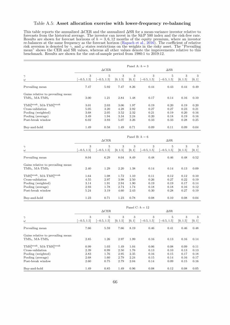
Table A.5: Asset allocation exercise with lower-frequency re-balancing

This table reports the annualized ∆CER and the annualized ∆SR for a mean-variance investor relative toforecasts from the historical average. The investor can invest in the S&P 500 index and the risk-free rate.Results are shown for forecast horizons of h = 3, 6, 12 months of the equity premium, where an investorre-balances at the same frequency as the forecast horizon (Rapach et al., 2016). The coefficient of relativerisk aversion is denoted by γ, and ω states restrictions on the weights in the risky asset. The ”Prevailingmean” shows the CER and SR values, whereas all other values denote the improvements relative to thisbenchmark. Results are shown for the out-of-sample period from 1980:1 to 2019:12.

Panel A: h = 3∆CER ∆SR

γ 3 5 3 3 3 5 3 3ω [−0.5, 1.5] [−0.5, 1.5] [0, 1.5] [0, 1] [−0.5, 1.5] [−0.5, 1.5] [0, 1.5] [0, 1]

Prevailing mean 7.47 5.92 7.47 8.26 0.44 0.43 0.44 0.49

Gains relative to prevailing mean:TMSt, MA-TMSt 3.00 1.21 2.84 1.48 0.17 0.14 0.16 0.10


t 3.01 2.03 3.06 1.97 0.19 0.20 0.19 0.20Cross-validation 5.05 3.20 4.28 2.92 0.27 0.27 0.23 0.21Pooling (weighted) 3.68 2.05 3.52 2.32 0.21 0.19 0.20 0.16Pooling (average) 3.49 1.94 3.34 2.24 0.20 0.18 0.19 0.16Post-break window 6.02 3.93 5.07 3.26 0.33 0.33 0.28 0.25

Buy-and-hold 1.49 0.58 1.49 0.71 0.09 0.11 0.09 0.04

Panel B: h = 6∆CER ∆SR

γ 3 5 3 3 3 5 3 3ω [−0.5, 1.5] [−0.5, 1.5] [0, 1.5] [0, 1] [−0.5, 1.5] [−0.5, 1.5] [0, 1.5] [0, 1]

Prevailing mean 8.04 6.29 8.04 8.49 0.48 0.46 0.48 0.52




Buy-and-hold 1.23 0.71 1.23 0.78 0.08 0.10 0.08 0.04

Panel C: h = 12∆CER ∆SR

γ 3 5 3 3 3 5 3 3ω [−0.5, 1.5] [−0.5, 1.5] [0, 1.5] [0, 1] [−0.5, 1.5] [−0.5, 1.5] [0, 1.5] [0, 1]

Prevailing mean 7.66 5.59 7.66 8.19 0.46 0.41 0.46 0.48




Buy-and-hold 1.49 0.85 1.49 0.96 0.08 0.12 0.08 0.05

66

Table A.6: Out-of-sample forecasting performance - Probit model

This table presents five forecast evaluation statistics for the out-of-sample recession probabil-ity forecasts, as well as the correlation between the probability forecasts and the (cumulative)log equity premium (ρ). The statistics are the quadratic probability score (QPS), logarithmscore (LS), diagonal elementary score (DES), pseudo R2, and the area under the receiver op-erating characteristic curve (AUROC). Results are shown for the probit model with TMSt and136

∑35j=0TMSt−j as predictors, and for five break-corrected versions of this probit model (Pe-

saran and Timmermann, 2007; Lettau and Van Nieuwerburgh, 2008). The recession probabilityforecasts refer to the probability that a recession occurs within the next h months. Results areshown for h = 1, 3, 6, 12 and the out-of-sample period is 1980:1 to 2019:12.

1980:1 to 2019:12

Variables in probit model QPS LS DES pseudo R2 AUROC ρ

Panel A: h = 1TMSt, MA-TMSt 0.17 0.27 0.05 0.27 0.92 -0.14


t 0.20 0.32 0.06 0.15 0.84 -0.13Cross-validation 0.15 0.23 0.03 0.35 0.94 -0.16Pooling (average) 0.17 0.26 0.04 0.29 0.92 -0.15Post-break window (15 years) 0.17 0.25 0.04 0.30 0.91 -0.18Post-break window (20 years) 0.14 0.22 0.04 0.37 0.94 -0.19

Panel B: h = 3TMSt, MA-TMSt 0.20 0.31 0.07 0.25 0.90 -0.22



Panel C: h = 6TMSt, MA-TMSt 0.22 0.36 0.09 0.25 0.87 -0.25



Panel D: h = 12TMSt, MA-TMSt 0.25 0.41 0.10 0.32 0.86 -0.37



67

Table A.7: Out-of-sample forecasting performance - Different lengths ofthe moving average component

This table presents five forecast evaluation statistics for the out-of-sample performance of theprobit model with the term spread and the moving average term spread as variables, as wellas the correlation between the probability forecasts and the (cumulative) log equity premium(ρ). The statistics are the quadratic probability score (QPS), logarithm score (LS), diagonalelementary score (DES), pseudo R2, as well as the area under the receiver operating characteristiccurve (AUROC). Results are shown for five different lengths of the moving average term spread,1l

∑l−1j=0TMSt−j , namely l = 12, 24, 36, 48, 60. The recession probability forecasts refer to the

probability that a recession occurs within the next h months. Results are shown for h = 1, 3, 6, 12and the out-of-sample period is 1980:1 to 2019:12.

1980:1 to 2019:12

Variables in probit model QPS LS DES pseudo R2 AUROC ρ

Panel A: h = 1l = 12 0.15 0.30 0.04 0.19 0.87 -0.08l = 24 0.15 0.23 0.02 0.34 0.93 -0.09l = 36 0.17 0.27 0.05 0.27 0.92 -0.14l = 48 0.19 0.31 0.07 0.16 0.87 -0.12l = 60 0.21 0.37 0.08 0.05 0.79 -0.12

Panel B: h = 3l = 12 0.16 0.33 0.05 0.21 0.86 -0.15l = 24 0.17 0.26 0.03 0.35 0.93 -0.19l = 36 0.20 0.31 0.07 0.25 0.90 -0.22l = 48 0.22 0.36 0.09 0.15 0.85 -0.19l = 60 0.23 0.41 0.09 0.05 0.76 -0.18

Panel C: h = 6l = 12 0.18 0.35 0.06 0.27 0.87 -0.22l = 24 0.19 0.30 0.05 0.37 0.91 -0.25l = 36 0.22 0.36 0.09 0.25 0.87 -0.25l = 48 0.24 0.40 0.09 0.16 0.83 -0.22l = 60 0.25 0.45 0.10 0.07 0.74 -0.20

Panel D: h = 12l = 12 0.18 0.35 0.06 0.44 0.90 -0.37l = 24 0.21 0.35 0.07 0.44 0.90 -0.40l = 36 0.25 0.41 0.10 0.32 0.86 -0.37l = 48 0.26 0.43 0.10 0.28 0.84 -0.33l = 60 0.27 0.46 0.11 0.21 0.78 -0.29

68

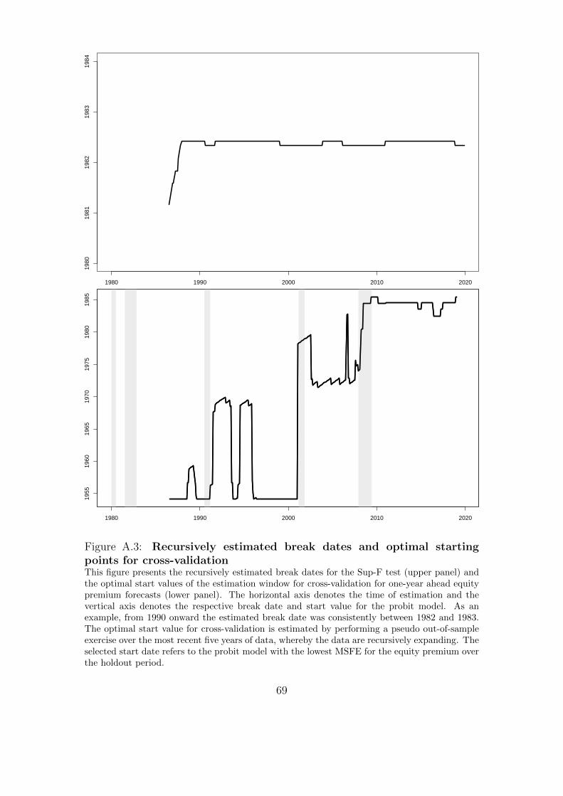
1980 1990 2000 2010 2020

1980

1981

1982

1983

1984

1980 1990 2000 2010 2020

1955

1960

1965

1970

1975

1980

1985

Figure A.3: Recursively estimated break dates and optimal startingpoints for cross-validationThis figure presents the recursively estimated break dates for the Sup-F test (upper panel) andthe optimal start values of the estimation window for cross-validation for one-year ahead equitypremium forecasts (lower panel). The horizontal axis denotes the time of estimation and thevertical axis denotes the respective break date and start value for the probit model. As anexample, from 1990 onward the estimated break date was consistently between 1982 and 1983.The optimal start value for cross-validation is estimated by performing a pseudo out-of-sampleexercise over the most recent five years of data, whereby the data are recursively expanding. Theselected start date refers to the probit model with the lowest MSFE for the equity premium overthe holdout period.

69

Table A.8: Estimated p-values with pre-whitening of standard errors

This table reports p-values for the null hypothesis of no structural break in the mean of the termspread. Ave-F, Exp-F, and Sup-F refer to the test statistics of Andrews (1993) and Andrews andPloberger (1994), and p-values are estimated by Hansen (1997). The standard errors are Neweyand West (1994) with an automatic bandwidth selection and different versions of pre-whitening.Results are shown for no pre-whitening of standard errors and for AR(1), AR(3), AR(6), andAR(12) pre-whitening of standard errors. The tests are carried out for trimming values of 15%(Panel A) and 5% (Panel B). The estimations are based on data from 1951:3 to 2019:12 and thebreak date refers to the global minimum in the sum of squared errors (Bai, 1997).

(1) (2) (3) (4) (5)

Ave-F Exp-F Sup-F break date

Panel A: 15% trimmingNo pre-whitening 0.00 0.00 0.00 1982:5AR(1) 0.06 0.04 0.01AR(3) 0.03 0.02 0.01AR(6) 0.01 0.01 0.01AR(12) 0.00 0.00 0.00

Panel B: 5% trimmingNo pre-whitening 0.00 0.00 0.00 1982:5AR(1) 0.07 0.05 0.02AR(3) 0.03 0.02 0.01AR(6) 0.01 0.01 0.02AR(12) 0.00 0.00 0.00

70

equity premium predictability over the business cycle

Documents