Erasmus University Rotterdam

Master Thesis

MSc International Economics

Russia: currency policy and its bilateral trade

Author: Supervisor:

Joey vd Hoeven Professor C. de Vries

20th of August, 2015

Abstract:

This paper attempts to identify the relationship between the bilateral trade balance of

Russia and its biggest trading partners, Germany and the USA, and several independent

explanatory variables. The empirical setup allows for non-stationarity and error

correction between the variables through the Vector Error Correction Model (VECM)

specification. This paper’s main conclusions are: (1) the Russian bilateral trade balance

and exchange rate do not show a long run relationship; and (2) the results indicate no J-

curve effect.

Index: Page(s):

1. Introduction 4 - 5

2. Literature review 6 - 9 2.1 Impact exchange rate on trade balance 6 - 7 2.2 Trade flows between countries 7 2.3 Effect oil - and gas price on Russian economy 8 2.4 J-curve effect 8 - 9 2.5 Econometric models 9

3. Sub – Question One 10 - 15

3.1 Period 1990 – 1993 10 3.2 Period 1995 – 2002 11 3.3 Period 2005 – 2008 12 - 13 3.4 Period 2009 – 2015 13 - 15

4. Sub – Question Two 16 - 19 4.1 Period 1991 – 1993 16 4.2 Period 1997 – 1999 16 - 18 4.3 Period 1999 – 2015 18 - 19

5. Sub – Question Three 20 - 42

5.1 Progressive scheme 20 - 23 5.2 Tests & results 23 - 42 5.2.1 Explanatory variables 30 5.2.2 Specifications 30 - 33 5.2.3Unit Root testing 33 - 34

5.2.4Engle-Granger cointegration approach 34 5.2.5Johansen cointegration test 35 5.2.6VECM 36 - 37 5.2.7VEC residual serial correlation LM test 37 - 38 5.2.8Heterskedasticity test VECM 38 5.2.9Pairwise Granger causality test 38 - 40 5.2.10Impulse response function 40 - 42

6. Conclusion 43 - 47

7. Bibliography 48 - 50

8. Appendices 51 - 129 Appendix A: Unit Root Tests 51 - 53 Appendix B: Serial Correlation Tests 54 - 63 Appendix C: Serial Correlation Tests Models USA 64 - 68 Appendix D: Serial Correlation Tests Models Germany 68 - 72

2

Appendix E: Trade Balance Regressions 73 Appendix F: Out of Sample Forecast Models 74 - 78 Appendix G: Seemingly Unrelated Regression (SUR) 79 Appendix H: Johansen Cointegration Tests 80 - 87 Appendix I: Vector Error Correction Estimates 88 - 93 Appendix J: OLS Estimates 94 - 97 Appendix K: LM Tests VECM 98 Appendix L: Heteroskedasticity Tests VECM 98 - 99 Appendix M: Impulse Graphs 100 - 103 Appendix N: Pairwise Granger Causality Tests 104 - 105 Appendix O: Augmented Dickey Fuller Test Residual VECM 106 - 108 Appendix P: Augmented Dickey Fuller Unit Root Tests

and Philips Perron Unit Root Tests 108 - 126 Appendix Q: Tables 126 - 129

3

1. Introduction:

Goldman Sachs published a research paper in 2002 about potential economic

superpowers of the 21th century (Purushothaman & Wilson, 2003). These potential

economic superpowers were summarized by the acronym BRIC (Brazil, Russia, India,

China). Based on this study, Russia was seen by many as an emerging superpower

economy and one of the most dominant economies “to be” in the middle of the current

century.

During the following years, Russia experienced some impressive economic growth,

with real gross domestic product (GDP) increasing 6.9% annually on average, which

helped to raise the Russian standard of living and brought economic stability (Cooper,

2009). However, the economic success of Russia was mainly based on high oil prices and

when the prices of both oil and other commodities went down in 2008, the Russian

economy suffered heavily. Both production and, even more importantly, export of oil and

gas went down rapidly (Cooper, 2009). On top of that the Russian economy was also, like

many other economies, hit substantially by the global financial crisis. The unavoidable

outcome of this all for Russia: Recession! (Cooper, 2009). In dealing with the

consequences of this crisis, Russia also had to make some important decisions regarding

its exchange rate policy.

The fact that Russia is an emerging economy and recently had to deal with a crisis

is one of the main reasons this paper focuses specifically on the Russian currency policy

before the financial crisis and the changing policy responses as a result of the crisis. To

prognose the amount of bilateral trade between Russia and Germany plus the USA

(Russia’s biggest trading partners), different models in EViews are used.

4

My main research question is:

How will the currency policy of Russia impact the international trade position of the country and

what do we predict to happen with the future bilateral trade between Russia, Germany and the

USA?

The findings of this main research question are underpinned by a few sub

questions. These sub-questions discuss what forms of currency policies were used in

Russia, how the Russian economy evolved over time and what I predict to happen with

the bilateral trade between Russia and its biggest trading partners, Germany and the

USA.

After above introduction, in which the purpose of this paper is explained, this paper

aims at answering the sub questions while making use of different data sources. The

answers of the sub questions will frame the insight of current policy impact, the potential

future effects on Russia’s international trade position and the possible future bilateral

trade between Russia, Germany and the USA. After that, findings, underpinned by

forecasting modeling results, are summarized and a clear conclusion is formulated.

5

2. Literature review:

The importance of the ”exchange rate” as an economic parameter is recognized by

many. The macro-economic impact of appreciation and/or depreciation is big in both

directly and indirectly impacted economies (Hashim & Zarma, 1996). The economic

parameter “exchange rate” is also often used to measure the economic performance of a

country and hence it is also seen as a crucial variable for policy decision making. The

stability of the exchange rate will allow the economic partners to plan well ahead with

stabile costs of production, but also with good oversight of expected prices for goods and

services. Very variable exchange rates, on the contrary, are seen by many as a main cause

of economic instability.

2.1 Impact exchange rate on trade balance:

The relationship (and mutual influence) of the “exchange rate” and the “trade

balance” variables has been studied for a long time. For that reason there is no shortage

of theoretical literature, describing and studying the inter-relation of the two parameters.

The literature describes a wide range of analyses and not in the last place because of the

economic importance of the inter-relation for the economic well being of countries. The

Mundell-Fleming model, a very popular model in this space, makes use of a IS-LM model

and enables the analysis of the economic impact of the exchange rate parameter on the

economy.

Stockman looked for a logical relationship between terms of trades (impacting

export/import) and the exchange rate. The model shows that both export/import and

exchange rate are simultaneously market driven and changes are triggered by supply and

demand step changes. The model does not suggest the two variables influencing each

other directly (Stockman, 1978).

The trade balance / exchange rate relationship was also examined by Shirvani and

Wilbratte. The specific case studied was between the USA and the 6 other G7 countries

being France, Italy, Germany, Japan, Canada and United Kingdom (Shirvani & Wilbratte,

6

1997). Akbostanci’s and Liu, Fan and Shek did case studies for respectively Turkey and

Honk Kong (Akbostanci, 2002; Liu, Fan, & Shek, 2007) .

Onafowora found a significant relationship in the bilateral trade of Malaysia,

Thailand and Indonesia with the USA and Japan. However, her test results didn’t proof a

significant relationship of exchange rate and trade balance. Again this conclusion is

important as it suggests that currency devaluation will not (positively) increase the long

term trade balance (Onafowora, 2003). In a similar study done by Liew, Lim, and

Hussain, focusing on ASEAN countries, their conclusion was that not the exchange rate

but real money had an impact on the trade balance (Liew, Lim, & Hussain, 2003).

The mentioned relationship real exchange rate / trade balance was studied by

Wilson and Kua for Singapore and the USA. Again the study confirmed no significant

mutual impact (Wilson & Kua, 2001).

A Thorbecke study showed an effect of an exchange rate change (appreciation) in 3

Asian countries (Malaysia, Indonesia and Thailand) actually would lead to a lower export

(Thorbecke, 2006).

On the contrary, Rose confirmed trade balance and exchange rate are not

significantly related. Hence, stimulating longer term trade balance numbers could not be

kicked off via exchange rate changes (Rose A. K., 1991)

2.2 Trade flows between countries:

The behaviour of trade flows between countries is important in economic

modelling and is being used in theoretical studies a lot. One can imagine that one of the

key contributing factors is the countries exchange rate. The establishment of the exchange

rate based on countries trade flows / pricing levels is deeply studied, amongst others by

Rey (Rey, 2001).

7

2.3 Effect of oil - and gas prices on Russian economy:

Basic trade statistics indicate that the EU imports a large percentage of it energy

products from Russia. Quantitative work on the effects of oil and natural gas on the

domestic Russian economy have been extensive. Tabata and Kuboniwa have made

significant steps in modeling the effects of Russian energy resources on other domestic

sectors, like the manufacturing industry, and the Russian economy as a whole (Tabata,

2011; Kuboniwa, 2010).

Furthermore, Rautava and Gaddy and Ickes have shown a lot of support for the

theory that the Russian business cycle can almost be fully explained by the fluctuations of

the international price of oil (Rautava, 2004; Gaddy & Ickes, 2010). All of this quantitative

work, however, is not isolated from the political area. Brugato correlated aggressive

Russian political maneuvers to fluctuations in the international price of oil. Brugato’s

paper quantitatively shows that the economics of oil and natural gas are inherently

linked to Russian politics (Brugato, 2008).

2.4 J-curve:

We are talking about a J-curve effect when a curve falls and eventually rises to a

point higher than the starting point, suggesting the letter J. An example of the J-curve

effect is seen when a country's trade balance initially worsens following a devaluation or

depreciation of its currency. The higher exchange rate will at first correspond to more

costly imports and less valuable exports, leading to a bigger initial deficit or a smaller

surplus. Due to the competitive, relatively low-priced exports, however, a country's

exports will start to increase. The trade balance eventually improves to better levels

compared to before devaluation.

8

As for literature on the J-curve effect, the findings do not give a clear support of it.

Some contradicting examples; Bahmani-Oskoee and Brooks found the J-curve / Marshall-

Lerner condition for the USA and their 6 major trading partners (Bahmani-Oskooee &

Brooks, 1991). However, Rose and Yellen could not confirm existence of the J-curve for

the USA, while Pesaran and Shin only confirmed the long term element of the J-curve

(Rose & Yellen, 1989; Pesaran, Shin, & Smith, 1996). In summary; conflicting conclusions

if it comes to confirming the J-curve for US international trade.

For developing countries (e.g. in Middle East and North Africa), the evidence of J-

curve existence was even more limited with Bahmani-Oskoee finding little short term J-

curve evidence and Upadhyaya and Dhakal showing support for a J-curve for only one

out of the 7 countries researched; Mexico (Bahmani - Oskooee, 2001; Upadhyaya &

Dhakal, 1997).

A widely used method concerning the J-curve effect is bilateral trade estimation.

This method looks at the trading flows of countries and how exchange rates influences

those flows The most investigated country in the literature is off course the USA. David

Backus investigated US/Canada trade in the 1970’s and found a J-curve pattern (Backus,

1986). Rey also looked at the USA-UK trade and found significant impact on trade

volumes of both money and financial markets (Rey, 2001).

2.5 Econometric models:

With the development of econometric modelling and econometric methods, VAR

and VEC models became popular in the field (Kale, 2001). A VAR model is used to

capture the linear interdependencies among multiple time series and a VECM adds error

correction features to this model in order to deal with the non-stationarity of some of the

series. Moffett studied the relationship between US import/export prices in relation to US

import/export quantities. The question was: is there a J-curve relationship? Results show

that a depreciation results in simultaneous decrease of exports and a decrease of imports

(Moffett, 1989).

9

3. Sub-question One:

How did the exchange rate policy of Russia develop over the years?

3.1 Period 1990 – 1993:

After the demise of the former Soviet Union, Russia implemented a floating

exchange rate system. This system was introduced because of the financial problems the

former Soviet union had, which started because of the sudden emergence of new nation

states without separate currencies and, thereby, with multiple central banks sharing a

common currency, without overall coordination or control (Sachs, 1996).

Like many other countries in the developing world, Russia experienced large

inflows and outflows of capital and was therefore increasingly subject to shocks coming

from world capital markets. Since the former Soviet Union didn’t have a lot of experience

with currency convertibility, monetary and exchange-rate policy had to be designed with

an eye toward currency stabilization (Sachs, 1996).

Even before reaching the decision over the exchange-rate regime, the successor

states to the Soviet Union had to take decisions regarding a national currency. In this, the

IMF made a serious mistake in early 1992, pushing hard for the continuation of a

common currency for the successor states, despite the existence of 15 separate central

banks and little feasibility of monetary coordination among the separate central banks.

The Russian government continued to accept the ruble credits issued by the non-Russian

central banks in payment for imports from Russia (Sachs, 1996).

In Russia, full monetary independence from the other states effectively began in

the fall of 1993, when Soviet currency notes were withdrawn from circulation in Russia,

and republics that still lacked their own currency finally moved to establish new national

currencies (Sachs, 1996).

10

3.2 Period 1995 – 2002:

Declining confidence in the domestic currency due to persistent inflation led to the

dollarization of the economy. To fight this, Russia introduced an exchange rate corridor

system in 1995, strengthening the role of the ruble exchange rate as the nominal policy

anchor (Central Bank of the Russian Federation, 2014). This didn’t have the effect they

were seeking since the nominal deficit averaged 7.4% of GDP during the three years

preceding the 1998 debt crisis (Edwards, 2001).

The government debt crisis of 1998 triggered a shift to a managed floating

exchange rate. After that crisis, exchange rate dynamics were largely market-driven and

allowed official reserves to be rebuilt as oil prices revived. The implementation of a

managed floating exchange rate system contributed to the smoothening of the influence

of changes in external conditions on the Russian financial markets, preventing excessive

movement in the ruble exchange rate, as this threatened macro-economic and financial

stability, and the Russian economy as a whole. This exchange rate policy also helped to

restore the confidence in the country’s financial system (Central Bank of the Russian

Federation, 2014). During the next years, Russia experienced an extraordinary economic

boost, despite the sharp downturn in the world economy as a whole.

The Bank of Russia intended to gradually decrease its influence on the exchange

rate dynamics and to shift to a floating exchange rate regime. However, the exchange rate

continued to be tightly managed through 2002–2005, mainly because of the fact that after

the East Asian, Russian and Brazilian crises, economists’ views on nominal exchange rate

regimes continued to evolve (Central Bank of Russia, 2014). Fixed-but-adjustable regimes

rapidly lost ground, while the two extreme positions, super-fixed, and freely floating

rates gained in popularity (Edwards, 2001).

11

3.3 Period 2005 – 2008:

In 2005, the Bank of Russia introduced a dual-currency basket as the operational

indicator for its exchange rate policy. Again, the aim was to smoothen the volatility of the

ruble’s exchange rate in relation to other major currencies. The dual-currency basket

consisted of the US dollar and the Euro (the value of the dual-currency basket is

calculated as the sum of ruble values of 0.55 US dollars and 0.45 Euro’s) and was

designed to keep the dynamics of the basket’s value in line with changes in the ruble’s

nominal effective exchange rate (Central Bank of Russia, 2014).

The global financial crisis of 2007-2008, as a result of bad housing loans by banks

around the world, led to a sharp decline in oil prices. This sharply eroded Russia’s

current account balance and triggered massive capital outflows, putting the ruble under

significant downward pressure. Dealing with the consequences of this crisis, Russia had

to make some important decisions regarding its exchange rate policy. Should the policy

aim to preserve the competitiveness gains associated with the ruble's devaluation by

making sure the exchange rate drops in line with inflation? Or is the calming effect of a

stable exchange rate on consumers and investors more important, even when Russian

producers begin to find it harder to compete against their foreign rivals? In other words,

is it better to have a "soft" ruble, or a "hard" one (Woodruff, 1999)? The legacy of Soviet

energy policy creates serious difficulties for either a hard ruble or a soft ruble policy.

When the ruble's dollar value is low, Russian energy users cannot afford to pay world

prices for oil and gas, or even a reasonable fraction of them. As a result, the government

comes under pressure to intervene in the economy and hold down energy prices. When

the ruble's dollar value is high, however, Russian firms cannot compete against foreign

firms.

12

The choice that Russia faced was whether to continue to combine a weak exchange

rate with export restrictions, or whether to pursue a strong exchange rate that would

make domestic energy sales attractive, but damage the competitiveness of the Russian

industry. If it wants to create a political base for long-term growth and eventually world

market competitiveness, Russia should choose a strong exchange rate. Such a policy has

one key advantage. This advantage is that it makes energy producers work all together to

generate growth (Woodruff, 1999). A stronger exchange rate would make the domestic

market a realistic source of major sales, leading energy producers to invest in their

customers in an effort to further expand the market. A weak exchange rate pits energy

exporters against the government in a battle over whether the domestic market will be

supplied at all; a strong exchange rate could unite the two forces in a battle for growth

(Woodruff, 1999). The bank of Russia decided to go for a policy that tried to create a

strong exchange rate, a trend that threatened to put a heavy strain on the balance sheets

of banks, the competitiveness of the Russian industry and households.

3.4 Period 2009 - 2015:

Between November 2008 and January 2009, the Bank of Russia allowed the ruble

to depreciate gradually by widening the dual-currency band. At the same time, the Bank

conducted large-scale interventions in the domestic foreign exchange market in order to

slow the pace of the ruble’s depreciation with the aim of giving the economy time to

adjust to these ongoing changes (Central Bank of the Russian Federation, 2014).

In January 2009, the Bank of Russia announced a wide fixed band for the ruble

value of the dual-currency basket (allowing fluctuations from 26 to 41 rubles) and it also

introduced a floating operational band. The gradual move to a more flexible exchange

rate regime was intended to create favorable conditions for market participants to adjust

to a fully floating exchange rate environment (Central Bank of the Russian Federation,

2014).

13

Starting from the first quarter of 2009, the exchange rate policy mechanism

permitted foreign exchange interventions both within the floating operational band for

the ruble value of the dual-currency basket and at its borders. The operational band

included a “neutral” range where no interventions were conducted. When the value of

the dual-currency basket moved outside the “neutral” range, the Bank of Russia started

buying or selling foreign currency. The closer the value of the dual-currency basket

approached the borders of the operational band, the more heavily the Bank of Russia

intervened. The Bank of Russia determined the volume of its target interventions

according to balance of payment factors, the budget policy and domestic and foreign

financial market conditions (Central Bank of the Russian Federation, 2014).

During 2009–2012, the Bank of Russia further increased the flexibility of its

exchange rate policy, widening the floating operational band from 2 to 7 rubles.

Following these changes, intervention volumes have steadily decreased. Yet the foreign

exchange market remained stable. This was caused by the fact that the gradual shift to a

more flexible Ruble exchange rate helped economic agents to adjust to the growing level

of Ruble volatility, promoting continued de-dollarisation, and making households’

foreign exchange deposits and foreign exchange cash purchases less vulnerable to Ruble

exchange rate changes. Also, the ruble’s volatility and exchange rate trends have stayed

in line with the dynamics of other emerging markets currencies (Central Bank of the

Russian Federation, 2014).

In 2013–2014, the Bank of Russia further increased the flexibility of the ruble

exchange rate regime with a view of creating the conditions for a transition to a fully

floating exchange rate regime by 2015. This was seen as an important requirement for the

introduction of inflation targeting. After moving to a floating exchange rate regime, the

Bank of Russia planned to abandon exchange rate-based operational indicators for its

exchange rate policy. Even in this case, however, the Bank retains the right to intervene in

the foreign exchange market (Central Bank of the Russian Federation, 2014).

14

From November 2014, the Bank of Russia finally abolished the exchange rate

policy mechanism through cancelling the range of the dual-currency basket ruble values

and regular interventions close to and outside the borders of this band. However, the

new approach of the Bank of Russia does not completely abandon foreign exchange

interventions, which can still be implemented in case of financial stability threats (Central

Bank of Russia, 2014).

During the first months of 2015, the Russian economy got into a dangerous

position. This was mainly caused by the fact that in one year the ruble’s value more than

halved against the dollar. A warning was given by the Central Bank of Russia that the

country’s GDP could decline by more than 4% should oil prices remain low. The decision

by the Central Bank of Russia to raise interest rates from 10.5% to 17% should

theoretically have helped to stabilize the Russian ruble. Instead, the currency weakened.

Since then, the ruble has been recouping its losses. However, the currency is still weak

and vulnerable to economic challenges and risks that the Central Bank of Russia is

fervently trying to mitigate. Despite Russia’s economic worries, the Central Bank of

Russia pressed ahead with fully floating the ruble, opening the currency up to the

pressures of floating freely in currency markets.

15

4. Sub-question Two:

How did Russia’s economic situation evolve over the years?

4.1 Period 1991 – 1993:

After the collapse of the Soviet Union in 1991 and the collapse of

Russia's controlled economy, a new Russian Federation was created under Boris Yeltsin.

He vowed to transform Russia's socialist economy into a capitalist market economy and

implemented economic shock therapy, price liberalization and nationwide privatization.

Due to a sudden total economic shift, a majority of the national property and wealth fell

into the hands of a small number of oligarchs. These oligarchs hindered commerce by

imposing unauthorized tolls and tariffs. Rather than creating new enterprises, Yeltsin's

democratization led to international monopolies hijacking the former Soviet markets,

arbitraging the huge difference between old domestic prices for Russian commodities

and the prices prevailing on the world market.

4.2 Period 1997 – 1999:

In the period 1997/1998 the Russian currency (Ruble) and the Russian economy

came into a vulnerable position. The main reason for that could be found in the so called

“oil crisis period” in which commodity prices (e.g. for oil and gas) went down

dramatically. As a result Russia was missing big foreign currency earnings. This put

downward pressure on Russia’s foreign currency reserves and made it more difficult to

service the debt and defend the ruble. In the same period, the Asian financial crisis kicked

in and investors did not want to take any risks in short term security holdings (Cooper,

2009).

16

With an economic system and related policies still based on a communistic history,

restructuring of policies was not a straightforward thing. Establishing a new tax regime

looked impossible. Bankruptcy laws could not be easily introduced. However, Russian

leadership was persistent to find the way forward and covert the central driven economy

into a more market driven economy. As described earlier, this change also made the

Ruble more “market driven” and internationally even opened the Russian economy

(Cooper, 2009).

In this period (end of the 90’s) quite some Russian banks, with some of them

holding government debt, collapsed. Many symptoms of the 1998 crisis developed even

before the financial crisis as Russian interest rates soared, prices on the Russian stock

market plummeted and the value of the Russian ruble sank (between July 1998 -

September 1998, 60% of its (nominal) value in terms of the dollar and an additional 17%

of its dollar value in the first nine months of 1999. The exchange rate reached 25 to 1, as

compared to 6.29 to 1 before the crisis). As a result of the many changes, the financial

reserves of Russia dropped in July/August 1998 with approximately 30% to $12,5 billion.

Russia’s GDP went down with almost 5% in 1998 (Cooper, 2009).

The core of the Russian crisis specifically was in fact that the government had to finance

budget deficits with short term debts. As long as the Russian governments could handle

these debts and deficits, the government was able to avoid inflation, and hence keep the

Ruble more or less stable.

The government also had to deal with a legacy from the (centrally planned)

economy of the past (e.g. period of Boris Yeltsin). Quite some ineffective, low quality,

non-competitive industries had to be abandoned or modernized in alignment with global

standards. Government expenditure in the Yeltsin period was massive with budget

deficits getting close to 10% of the GDP. Extreme high interest rates had to be paid to

17

finance these government debts. The radical approach in Yeltsin’s reform program

created inflation as the market economy got introduced a bit too early (Cooper, 2009).

The massive devaluation of the ruble had some positive effects for the economy.

With their rubles worth fewer dollars, Russians were no longer able to afford imported

goods. They began to look for domestically produced alternatives, and many Russian

businesses responded with a lot of enthusiasm. Russian exporters also benefited, because

their costs for wages and other domestic inputs fell greatly in dollar terms, making them

more competitive on world markets (Woodruff, 1999).

It was widely feared, however, that the positive effects of devaluation would be

short-lived. Opportunities to replace imports had largely already been realized.

Meanwhile, inflation was starting to outstrip the continuing decline in the exchange rate.

As a result, Russian prices were going up in dollar terms, eroding earlier competitiveness

gains (Woodruff, 1999).

4.3 Period 1999 – 2015:

During the period 1999 – 2008, the Russian economy experienced a great 6,9%

increase of the real GDP (Cooper, 2009). With that excellent average, not only did the

Russian standard of living increase, but both economic and financial stability increased

and that was something that Russia missed for a long period (Cooper, 2009). The impact

of this success on political leaders (like Putin and Dmitrij Medvedev) was very positive

and they gained the support of the Russian people even more. This allowed them to re-

position Russia again as world power, next to Europe and the USA (Cooper, 2009).

By the end of 2008 also the Russian economy started to suffer, like all other

economies, from a recession as a result of the (global) financial crisis. Many industrial

countries had a big dependency on the huge amount of natural reserves in Russia (oil,

gas, etc.) and these reserves sales did boost Russia’s economy in the economic growth

period (Cooper, 2009). But now, with recession kicking in, the need for oil, gas and other

18

raw materials disappeared. The Russian economy showed to have become too dependent

on the income from oil and other commodities. This caused great instability from 2008

onwards. The biggest collapse came in the summer of 2014, when these resources lost

50% of their value, hitting the Russian economy hard.

In order to reduce the capital outflows, slow the ruble’s depreciation and to

prevent instability in domestic financial markets, the Bank of Russia raised interest rates

steadily and implemented a range of additional measures. Banks were advised to

maintain stable levels of net foreign assets and currency positions, and their observance

of these recommendations was taken into account when credit limits were set for

individual banks’ access to Bank of Russia unsecured loans. Limits were substantially

reduced for banks that did not adequately respect the recommendations (Central Bank of

the Russian Federation, 2014).

19

5. Sub-question Three:

What do we predict to happen with the future bilateral trade between Russia, Germany and the

USA?

This sub question is answered with the help of a progressive scheme. This scheme goes

through the different steps that are necessary to predict the net trade between Russia and

Germany plus the USA. These predictions are the input to various forecasting models (to

be explained in further detail). Simulation tests are computed and result in a hypothesis.

Further analysis of the simulation output leads to a better estimation of the different

forecasting models. This analysis allows a comparison of strengths of the different

models used. Ultimately the best fit model is used to answer this specific sub question.

5.1 Progressive Scheme:

The statistical program EViews is being used to calculate/ predict the net amount of trade

between Russia, Germany and the USA. EViews is a specialized program to do analysis

over time series. The (Russian Ruble/US$) exchange rate is one of the variables I use to

predict the future Russian bilateral trade, as a change of the exchange rate has a effect on

the bilateral trade balance. It is assumed that a depreciation of the real exchange rate

leads to an improvement of the bilateral trade balance of a country. The logic behind this

is that export goods become less expensive for the outside world, which in turn

encourage other countries to buy more goods. The second variable that I use is the Gross

Domestic Product (GDP) of Russia. An increase in the Russian income is likely to have a

(negative) effect on the bilateral trade balance. It is likely that the Russian imports will

increase if income increases and have a effect on the bilateral trade balance. The Gross

Domestic Product (GDP) of the USA is the third variable I am using. This country’s GDP

is chosen as variable as it is the largest importer of Russian goods. An increase in the

GDP of the USA will therefore have a positive effect on the bilateral trade balance. The

Gross Domestic Product (GDP) of Germany is the fourth variable. This because of the fact

that Germany is one of the biggest trading partners of Russia. As stated before: Russia is

20

one of the biggest/ largest owners of natural reserves. Beside former Soviet States, other

big consumers of the reserves (like Germany and the USA) are also dependent on these

Russian reserves. Hence I also used both the prices of gas and oil. The associated variable

names for my research are:

-- Trade_balance_us = net trade between the USA and Russia (exports USA to

Russia – imports USA from Russia)

-- Trade_balance_ger = net trade between Germany and Russia (exports

Germany to Russia – imports Germany from Russia)

-- GDP_Russia = the GDP of Russia

-- GDP_Us = the GDP of the USA

-- GDP_Ger = the GDP of the Germany

-- Exchange_eu = the (Russian Ruble/EU€) exchange rate

-- Exchange_us = the (Russian Ruble /US$) exchange rate

-- Oil_price = the oil price

-- Gas_price = the gas price

The dataset that I use for these variables consists of monthly GDP of Russia data,

monthly GDP of the USA data and monthly GDP of Germany data from at least the year

2000 until 2014, daily (Russian Ruble /US$ and Russian Ruble/EU€) exchange rate data

and converting this into monthly data, and monthly oil price and gas price data.

Before starting a regression analysis, one needs to validate that the variables that go into

the analysis are stationary. Non-stationary variables have the risk that the computed

regression are worthless/random. The results in those cases might suggest a (significant)

relationship which is totally non-existing. The Augmented Dickey Fuller test can be used

to check if a variable is really stationary. For those cases that variables proof to be non-

stationary, one can still look for stationary variables by taking the first difference; so we

test the lagged variables for stationarity. If needed we can apply the next level difference

to finally get a stationary variable.

21

Assuming that we now have checked on stationarity and have found our

stationary variables, we also need to do some other checks. The independent variables

that we want to apply in the model also need to meet the assumptions of “Ordinary Least

Squares”. Not meeting these assumptions leads to an unbiased regression and hence to

incorrect regression results. The “Ordinary Least Squares” assumptions used are:

• “Homoscedasticity”; the variance of the error term has to be constant.

Homoscedasticity can be checked by using the residual plot and see if the

errors are varying constantly.

• “Normality”; the error term is normally distributed. Normality can be

checked by making use of the histogram functionality and then see if the

histogram meets a normal distribution.

• “Linearity”; the dependent and independent variables have a linear

relationship to each other. To validate linearity one makes use of a so called

scatterplot. If the scatterplot form meets a line, there is linearity.

• ”no serial correlation”; the error term is uncorrelated to itself. Serial

correlation can be checked by creating a so called correlogram. Using a

correlogram, probabilities show serial correlation or not

Now that I have checked the variables on stationarity and the OLS assumptions, I am

ready to start using the different forecasting models. For the forecasting quality it is

crucial that the dependent variable is “lagged”. In other words; the dependent variable

should reflect a year on year change. Furthermore it is important re-iterate that when

running the different forecasting models, none of them should have serial correlation

between the errors.

22

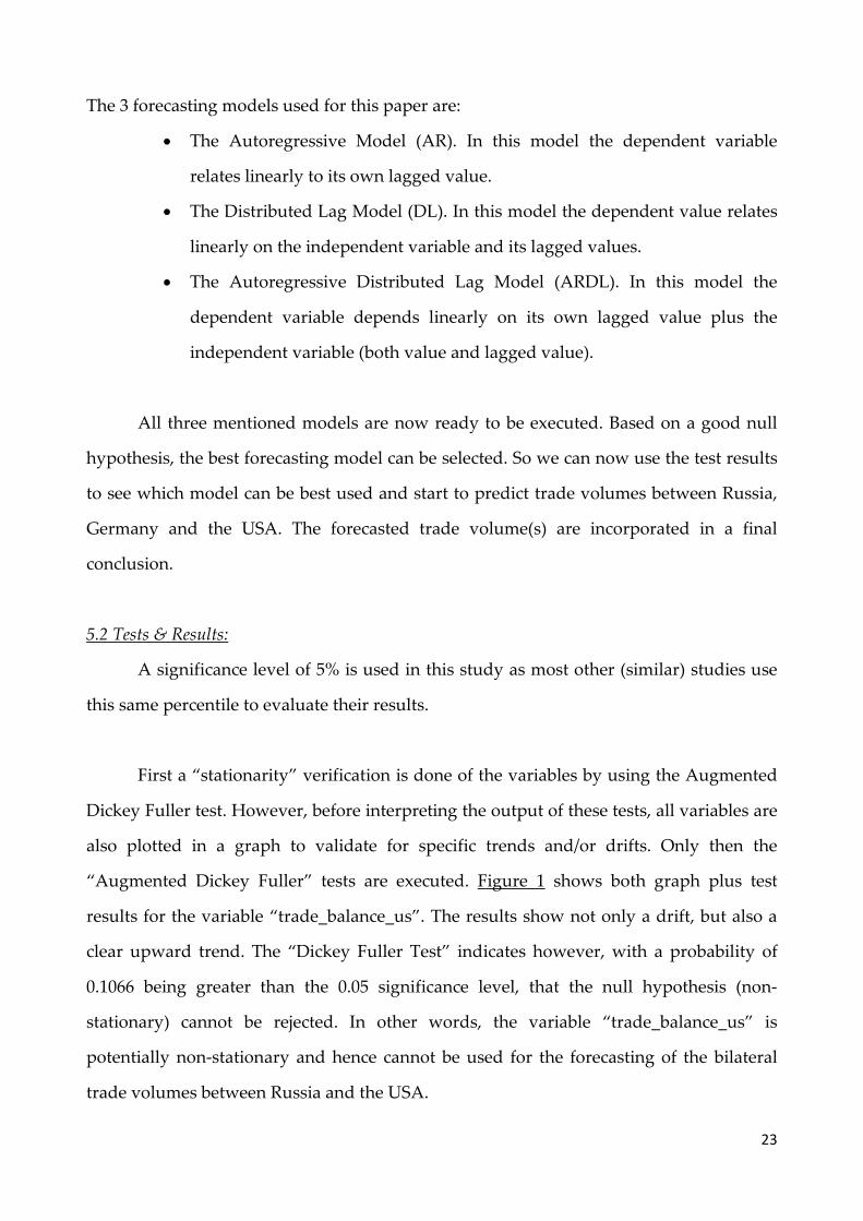
The 3 forecasting models used for this paper are:

• The Autoregressive Model (AR). In this model the dependent variable

relates linearly to its own lagged value.

• The Distributed Lag Model (DL). In this model the dependent value relates

linearly on the independent variable and its lagged values.

• The Autoregressive Distributed Lag Model (ARDL). In this model the

dependent variable depends linearly on its own lagged value plus the

independent variable (both value and lagged value).

All three mentioned models are now ready to be executed. Based on a good null

hypothesis, the best forecasting model can be selected. So we can now use the test results

to see which model can be best used and start to predict trade volumes between Russia,

Germany and the USA. The forecasted trade volume(s) are incorporated in a final

conclusion.

5.2 Tests & Results:

A significance level of 5% is used in this study as most other (similar) studies use

this same percentile to evaluate their results.

First a “stationarity” verification is done of the variables by using the Augmented

Dickey Fuller test. However, before interpreting the output of these tests, all variables are

also plotted in a graph to validate for specific trends and/or drifts. Only then the

“Augmented Dickey Fuller” tests are executed. Figure 1 shows both graph plus test

results for the variable “trade_balance_us”. The results show not only a drift, but also a

clear upward trend. The “Dickey Fuller Test” indicates however, with a probability of

0.1066 being greater than the 0.05 significance level, that the null hypothesis (non-

stationary) cannot be rejected. In other words, the variable “trade_balance_us” is

potentially non-stationary and hence cannot be used for the forecasting of the bilateral

trade volumes between Russia and the USA.

23

To get this variable “stationary”, the first difference is taken, i.e. the difference between

the bilateral trade this year and the bilateral trade last year. This variable is shown as “d_

trade_balance_us = trade_balance_us – trade_balance_us (-1)”. Figure 2 shows the test

results (and graph) for this “first difference” variable (d_ trade_balance_us) and in this

case the null hypothesis can clearly be rejected. The probability of 0.0000 is clearly below

the 0.05 significance level. So the “non-stationary” null hypothesis is rejected and the

variable “d_ trade_balance_us” is deemed to be stationary. The mentioned variable can

be used in the forecasting models.

All the other variables are tested in similar fashion and are all stationary when using the

first difference. Details on this analysis can be found in Appendix A. Working with a

model is easier if all variables are lagged in the same order. In my study I therefore used

a lagging of the first order. The first order lagging that I use in all my models will not

impact the variables “stationarity”. As the graph shows; lagging will not turn a

“stationary” in a “non-stationary” variable.

Now it is time to execute the checks on the OLS assumptions. I now regress the “lagged

bilateral trade” variable with the lagged variables of the GDP of Russia, the GDP of the

USA and Germany plus the ones of the oil price and the gas price. Mentioned regressions

are shown below:

After computing the tests for “homoscedasticity”, “normality”, “linearity” and

“serial correlation”, output results show that all of these assumptions are not violated if I

24

look at the bilateral trade balance between Russia and Germany, and most of these

assumptions are not violated if I look at the bilateral trade balance between Russia and

the USA (appendix B). Still there is a small amount of violations in the USA case, which

could cause the regression’s output to be biased in some (small) way.

As stated in section 5.1 (progressive scheme), three forecasting models are being used in

this paper:

• The AR Model

• The DL Model

• The ARDL Model

For reference, mentioned models and their specifics are summarized in 5.1.

So what do we expect as potential outcome of our modeling activities? One would

expect Russia’s GDP to have a high influence on trading amount with both the USA and

Germany. As the increase of Russia’s GDP would naturally lead to the willingness of

Russia to increase the imports from economic partners like the USA and Germany; off

course the change will impact the amounts of trade between mentioned countries.

With the use of more variables (5 in my study) I can strengthen the null hypothesis,

which now becomes:

The ARD (Autoregressive Distribution) Lag Model with the 5 variables (1) lagged trade balance;

(2) lagged exchange rate; (3) lagged Russian GDP; (4) lagged oil price and (5) the lagged gas price

is best to forecast net Russian bilateral trading amounts with Germany and the USA.

The forecasting models used to predict trade volumes between Russia and Germany plus

the USA make use of the following variables:

• “d_exchange_us”

• “d_exchange_eu”

• “d_gdp_russia”

• “d_ trade_balance_us”

25

• “d_ trade_balance_ger”

• “d_oil_price”

• “d_gas_price”

The regression formulas of the AR, DL and ARDL Models are shown in the following

overview:

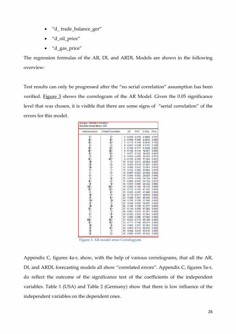
Test results can only be progressed after the “no serial correlation” assumption has been

verified. Figure 3 shows the correlogram of the AR Model. Given the 0.05 significance

level that was chosen, it is visible that there are some signs of “serial correlation” of the

errors for this model.

Figure 3. AR model error Correlogram

Appendix C, figures 4a-r, show, with the help of various correlograms, that all the AR,

DL and ARDL forecasting models all show “correlated errors”. Appendix C, figures 5a-r,

do reflect the outcome of the significance test of the coefficients of the independent

variables. Table 1 (USA) and Table 2 (Germany) show that there is low influence of the

independent variables on the dependent ones.

26

Data from table 1 indicates that the AR-model is the best model that can be used to

predict the future value of the bilateral trade between Russia and the USA, since it is the

only model in which all the parameters are significant. The conclusion for these tables is

clear: Russian bilateral trade volumes can be best forecasted based on last year trade

numbers complemented with a constant value (the AR model). Looking at the data in

table 1, it is interesting to see that the first difference of the previous oil price (variable

“d_oil_price(-1)”) is significant in most of the models, but isn’t included in the model that

predicts the best. I therefore wanted to take a look at a model that contained both the

variable “d_trade_balance_us(-1)” and the variable “d_oil_price(-1)”. The output of this

model can be seen in appendix E. The output shows that the bilateral trade between

Russia and the USA can also be predicted really well with a model that consists of the

previous bilateral trade balance and the previous oil price. Since this was the case for the

bilateral trade between Russia and the USA, I also wanted to take a look at the Germany

case. The output of this model is also shown in appendix E. This output shows a different

situation, since the previous oil price isn’t significant here and therefore the AR model, as

shown in table 2, is still the best model to predict the future bilateral trade balance

between Russia and Germany.

Out of sample forecasts have been done for the various models. As can be seen in

appendix F, most of these out of sample forecasts are not good, since the important

parameters “bias proportion”, indicating how far the mean is from the mean of the actual

series, and “variance proportion”, indicating how far the variance of the forecasts is from

the variance of the actual series, are both not small. In order to have a good out of sample

forecast, both of these parameters should be small. The results indicate that in all the

forecasts the “bias proportion” is always really small, but they also indicate that the

“variance proportions” of all the out of sample forecasts are really high. The only cases

for which could be stated that the “variance proportions” are relatively low is when we

look at the out of sample forecasts of the ARDL3 and ARDL4 models, but even then the

“variance proportion” has a pretty high value. Taking this all into account, we can

conclude that the out of sample forecasts are not good.

27

I also want to look if the bilateral trade balance between Russia and Germany is

correlated with the bilateral trade balance between Russia and the USA. I did this with

the use of a Seemingly Unrelated regression (SUR). A SUR is used to gain efficiency in

estimation by combining information on different equations and it is used to impose

and/or test restrictions that involve parameters in different equations. I use both the

equation of the dependent variable “d_trade_balace_us” as the equation of the dependent

variable “d_trade_balance_ger”. The output of this SUR is shown in appendix G. The

output shows that the equations of “d_trade_balance_ger” and of “d_trade_balance_us”

are not correlated, since the correlation value is really small. Because of this, the VEC

models are predicted separately.

5.2.1 Explanatory variables::

I also examine the relationship between the different components of the Russian

bilateral trade balance with the US and Germany. As mentioned before, the variables that

I consider are the Russian GDP, the US GDP, the German GDP, the oil price, the gas

price, the real exchange rate between the Russian Ruble and the American Dollar and the

real exchange rate between the Russian Ruble and the Euro. I follow the structure and

methodology of Yeun-Ling, Wai-Mun, & Geoi-Mei closely (Yuen-Ling, Wai-Mun, & Geoi-

Mei, 2008).

First the relationship between the different components is estimated with a

ordinary least squares regression (OLS). The main objective is to explain the dependent

variables “lgtrade_balance_us” and “lgtrade_balance_ger” with the variables “Russian

28

GDP”, “US GDP”, “German GDP”, “oil price”, “gas price” and the “real exchange rate”

(Russian Ruble /US$ and Russian Ruble/EU€), with particular interest for the effect of the

real exchange rate on the Russian bilateral trade balance with the US and Germany.

The natural logarithms (ln) of all variables are taken. Due to this transformation

the variables could be interpreted as elasticity’s.

5.2.2 Specifications:

The following two regressions are being used:

(1) 𝑙𝑙𝑙𝑙𝑙𝑙𝑙𝑙𝑙𝑙𝑙𝑙𝑙𝑙_𝑏𝑏𝑙𝑙𝑙𝑙𝑙𝑙𝑏𝑏𝑏𝑏𝑙𝑙_𝑢𝑢𝑢𝑢 = 𝛽𝛽0 + 𝛽𝛽1𝑙𝑙𝑙𝑙𝑙𝑙𝑙𝑙𝑝𝑝𝑅𝑅𝑅𝑅𝑅𝑅𝑅𝑅𝑅𝑅𝑅𝑅 + 𝛽𝛽2𝑙𝑙𝑙𝑙𝑙𝑙𝑙𝑙𝑝𝑝𝑈𝑈𝑈𝑈 + 𝛽𝛽3𝑙𝑙𝑙𝑙𝑙𝑙𝑙𝑙𝑏𝑏ℎ𝑙𝑙𝑏𝑏𝑙𝑙𝑙𝑙_𝑢𝑢𝑢𝑢 + 𝛽𝛽4𝑙𝑙𝑙𝑙𝑙𝑙𝑙𝑙𝑙𝑙_𝑝𝑝𝑙𝑙𝑙𝑙𝑏𝑏𝑙𝑙 +

𝛽𝛽5𝑙𝑙𝑙𝑙𝑙𝑙𝑙𝑙𝑢𝑢_𝑝𝑝𝑙𝑙𝑙𝑙𝑏𝑏𝑙𝑙 + µ

(2) 𝑙𝑙𝑙𝑙𝑙𝑙𝑙𝑙𝑙𝑙𝑙𝑙𝑙𝑙_𝑏𝑏𝑙𝑙𝑙𝑙𝑙𝑙𝑏𝑏𝑏𝑏𝑙𝑙_𝑙𝑙𝑙𝑙𝑙𝑙 = 𝛽𝛽0 + 𝛽𝛽1𝑙𝑙𝑙𝑙𝑙𝑙𝑙𝑙𝑝𝑝𝑅𝑅𝑅𝑅𝑅𝑅𝑅𝑅𝑅𝑅𝑅𝑅 + 𝛽𝛽2𝑙𝑙𝑙𝑙𝑙𝑙𝑙𝑙𝑝𝑝𝑔𝑔𝑔𝑔𝑔𝑔𝑔𝑔𝑅𝑅𝑔𝑔𝑔𝑔 + 𝛽𝛽3𝑙𝑙𝑙𝑙𝑙𝑙𝑙𝑙𝑏𝑏ℎ𝑙𝑙𝑏𝑏𝑙𝑙𝑙𝑙_𝑙𝑙𝑢𝑢 +

𝛽𝛽4𝑙𝑙𝑙𝑙𝑙𝑙𝑙𝑙𝑙𝑙_𝑝𝑝𝑙𝑙𝑙𝑙𝑏𝑏𝑙𝑙 + 𝛽𝛽5𝑙𝑙𝑙𝑙𝑙𝑙𝑙𝑙𝑢𝑢_𝑝𝑝𝑙𝑙𝑙𝑙𝑏𝑏𝑙𝑙 + µ

These regressions tell that the relative exports to imports between Russia and its

biggest trading partners, the USA and Germany, are explained by the GDP of the

countries, the real exchange rate and the oil and gas prices.

All variables in equation (1) and (2) are tested for stationarity. In addition to the

paper of Yeun-Ling, Wai-Mun, & Geoi-Mei, the Augmented Dickey-Fuller (ADF) test and

the Philips-Perron (PP) tests are used for unit root testing (Yuen-Ling, Wai-Mun, & Geoi-

Mei, 2008). If both tests give opposing results for a variable, the KPSS test is used to

decide if there is a unit root. Testing for unit root is important because non-stationary

variables can cause some problems to standard OLS regression. As can be seen in

Appendix P, I find a unit root in almost all variables using the ADF test and the PP test.

Since this is undesirable for regression analysis, the first difference is taken from all

variables. The US regression now has the following form:

(3) 𝐷𝐷(𝑙𝑙𝑙𝑙𝑙𝑙𝑙𝑙𝑙𝑙𝑙𝑙𝑙𝑙_𝑏𝑏𝑙𝑙𝑙𝑙𝑙𝑙𝑏𝑏𝑏𝑏𝑙𝑙_𝑢𝑢𝑢𝑢) = 𝛽𝛽0 + 𝛽𝛽1𝐷𝐷(𝑙𝑙𝑙𝑙𝑙𝑙𝑙𝑙𝑝𝑝_𝑅𝑅𝑢𝑢𝑢𝑢𝑢𝑢𝑙𝑙𝑙𝑙) + 𝛽𝛽2𝐷𝐷(𝑙𝑙𝑙𝑙𝑙𝑙𝑙𝑙𝑝𝑝_𝑈𝑈𝑈𝑈) +

𝛽𝛽3𝐷𝐷(𝑙𝑙𝑙𝑙𝑙𝑙𝑙𝑙𝑏𝑏ℎ𝑙𝑙𝑏𝑏𝑙𝑙𝑙𝑙_𝑢𝑢𝑢𝑢)+ 𝛽𝛽4𝐷𝐷(𝑙𝑙𝑙𝑙𝑙𝑙𝑙𝑙𝑙𝑙_𝑝𝑝𝑙𝑙𝑙𝑙𝑏𝑏𝑙𝑙) + 𝛽𝛽5𝐷𝐷(𝑙𝑙𝑙𝑙𝑙𝑙𝑙𝑙𝑢𝑢_𝑝𝑝𝑙𝑙𝑙𝑙𝑏𝑏𝑙𝑙) + µ

29

D stands for the first difference of the variable. Taking the first difference is a standard

routine to get rid of unit root in variables in order to use the variables in a regression

analysis.

Another way to cope with non-stationary variables which are integrated of order

one ( that is after taking the first difference the variables are stationary), is to look at the

cointegration of the variables. I examine the cointegration relationship between the

variables by using the Engle-Granger approach and the Johansen cointegration test.

The Engle-Granger approach requires two steps to be taken. The first step is again

to estimate the regression (1 and 2) and obtain the residual term µ from the equation. The

second step is to perform a standard ADF unit root test on the residual term µ to see if

this term is stationary. In order to say that the variables are cointegrated, the residual

term µ should form a stationary serie. However, it could be argued that there are some

problems with the Engle-Granger approach. One of these problems is that the residual

series is estimated rather than observed, so the standard asymptotic distributions of

conventional unit root statistics do not apply. Therefore I apply another cointegration test

to see if the variables are cointegrated.

The Johansen cointegration test was used in order to determine the number of

cointegration relationships between the variables. Determining this number of

cointegration relationships is important, especially for the next step taken in this analysis.

This next step is the Vector error correction model (VECM).

The VECM model shows if a lagged value (Lag one and Lag two) of the variables

are significantly explaining the dependent variables in the VECM model. This is

interesting since the long run relationship between the variables could be revealed. The

30

VECM is also important for our analyses because it serves as the basis for the impulse

response function.

Following Yeun-Ling, Wai-Mun, & Geoi-Mei, statistical tests are applied on the

VECM model to verify the correctness of the model (Yuen-Ling, Wai-Mun, & Geoi-Mei,

2008). The model is tested for serial correlation, hetroskedasticity and the pairwise

Granger causality test is applied on the model. With this causality test I can elicit the

direction in which the variables influence each other.

To analyze the short run and long run effects of one variable on another, an

impulse response function is conducted. The impulse response function shows the effect

of a change in one variable on another variable and also show how that effect behaves

over time. This is interesting to see, because it is usually assumed that a depreciation of

the real exchange rate (“exchange_us” or “exchange_eu”) first decreases the value of the

trade balance, that is imports increase relatively to exports, and later on improve the

trade balance; the so called J-Curve. With the impulse response function I can extend our

analysis and I could investigate the existence of the J-Curve for the Russian trade balance.

The estimates of regression equation (3) are summarized in table 3 of appendix Q.

The estimated parameter values are:

𝐷𝐷(𝑙𝑙𝑙𝑙𝑙𝑙𝑙𝑙𝑙𝑙𝑙𝑙𝑙𝑙_𝑏𝑏𝑙𝑙𝑙𝑙𝑙𝑙𝑏𝑏𝑏𝑏𝑙𝑙_𝑢𝑢𝑢𝑢) = 43.36815− 0.403572𝐷𝐷(𝑙𝑙𝑙𝑙𝑙𝑙𝑙𝑙𝑝𝑝𝑅𝑅𝑅𝑅𝑅𝑅𝑅𝑅𝑅𝑅𝑅𝑅) − 0.271563𝐷𝐷(𝑙𝑙𝑙𝑙𝑙𝑙𝑙𝑙𝑝𝑝𝑈𝑈𝑈𝑈) −

0.929540𝐷𝐷(𝑙𝑙𝑙𝑙𝑙𝑙𝑙𝑙𝑏𝑏ℎ𝑙𝑙𝑏𝑏𝑙𝑙𝑙𝑙_𝑢𝑢𝑢𝑢) + 0.017614𝐷𝐷(𝑙𝑙𝑙𝑙𝑙𝑙𝑙𝑙𝑙𝑙_𝑝𝑝𝑙𝑙𝑙𝑙𝑏𝑏𝑙𝑙) + 0.035239𝐷𝐷(𝑙𝑙𝑙𝑙𝑙𝑙𝑙𝑙𝑢𝑢_𝑝𝑝𝑙𝑙𝑙𝑙𝑏𝑏𝑙𝑙) + µ

5.2.3 Unit root testing:

Both the “Augmented Dickey Fuller” test and “Philips Perron”unit root tests are

being used to check for the existence of a unit root. Most variables don’t have a unit root

according to the ADF test and the PP test, except for the variables “lgexchange_eu”,

“lggdp_US”, which has a unit root according to all the tests, except the PP test with trend,

the variable “lgexchange_us”, the variable “lgoil_price” and the variable “lggas_price”

(for all tests except the ADF test with trend). After taking the first difference all variables

31

are stationary. This is, as said before, important since variables with a unit root can give

rise to serious problems with the OLS estimator. After these tests I can conclude that this

is not the case with this regression, because all variables are at most integrated of order

one (1). This means that the variables are stationary after taking the first difference. In

table 3 and 4 (4 & 5 in appendix Q) the results of the ADF and PP tests are summarized.

Table 3. ADF & PP (USA)

Table 4. ADF & PP (Germany)

5.2.4 Engle-Granger cointegration approach:

Variable ADF test PP test KPSS test No trend Trend No trend Trend Lggdp_russia 0.0035 3 0.0009 3 0.0035 3 0.0009 3 D(Lggdp_russia) 0.0000 3 0.0000 3 0.0000 3 0.0001 3 Lggdp_US 0.8091 0.2882 0.7978 0.0004 3 Unit root D(lggdp_US) 0.0000 3 0.0000 3 0.0000 3 0.0000 3 Lgexchange_us 0.9805 0.9849 0.9988 0.9990 D(lgexchange_us) 0.0000 3 0.0000 3 0.0000 3 0.0000 3 Lgtrade_balance_us 0.0031 3 0.0000 3 0.0000 3 0.0000 3 D(lgtrade_balance_us) 0.0000 3 0.0000 3 0.0001 3 0.0001 3 Lgoil_price 0.3380 0.3233 0.4380 0.4881 D(Lgoil_price) 0.0000 3 0.0000 3 0.0000 3 0.0000 3 Lggas_price 0.6528 0.0311 2 0.7477 0.1392 D(Lggas_price) 0.0000 3 0.0000 3 0.0000 3 0.0000 3 1 = 10% ; 2 = 5% ; 3 = 1% significance level

Variable ADF test PP test KPSS test No trend Trend No trend Trend Lggdp_russia 0.0035 3 0.0009 3 0.0035 3 0.0009 3 D(Lggdp_russia) 0.0000 3 0.0000 3 0.0000 3 0.0001 3 Lggdp_ger 0.0000 3 0.0000 3 0.0000 3 0.0000 3 D(lggdp_ger) 0.0000 3 0.0000 3 0.0000 3 0.0000 3 Lgexchange_eu 0.9516 0.5674 0.9935 0.9488 D(lgexchange_eu) 0.0000 3 0.0000 3 0.0000 3 0.0000 3 Lgtrade_balance_ger 0.0000 3 0.0000 3 0.0000 3 0.0000 3 D(lgtrade_balance_ger) 0.0000 3 0.0000 3 0.0000 3 0.0000 3 Lgoil_price 0.3380 0.3233 0.4380 0.4881 D(Lgoil_price) 0.0000 3 0.0000 3 0.0000 3 0.0000 3 Lggas_price 0.6528 0.0311 2 0.7477 0.1392 D(Lggas_price) 0.0000 3 0.0000 3 0.0000 3 0.0000 3 1 = 10% ; 2 = 5% ; 3 = 1% significance level

32

I now continue with the Engle-Granger cointegration approach. The residual term

µ (called RESIDUAL1) is tested for unit root with an ADF test with trend and intercept.

The t-statistic for this ADF test for the USA case on the residual is -9.565347 and the

corresponding p-value is 0.0000. The t-statistic for this ADF test for the Germany case on

the residual is -1.161536 and the corresponding p-value is 0.6764. However, since the

ADF test is now used to test for co-integration in the residual term, the standard p-value

provided in Eviews is incorrect. Therefore the t-values (-9.565347 (USA) / -1.161536

(Germany)) of the ADF tests are compared with critical values obtained from “Critical

values for cointegration tests” (MacKinnon, 2010). The critical value for the 5%

significance level is -4.43 and therefore we do reject the null hypothesis in the USA case.

This means that there is no unit root, that the residual term is stationary and that the

variables are cointegrated. In the case of Germany I do not reject the null hypothesis. This

means that there is a unit root, that the residual term is not stationary and that the

variables are not cointegrated. These results can also been seen in tables 6 and 7 in

appendix Q.

5.2.5 Johansen cointegration test:

The Johansen cointegration test is used to determine the number of cointegration

relationships between the variables. The Johansen test actually performs two different

methods in explaining the number of cointegration relationships. Namely the trace value

and the maximum eigenvalue. The trace value test indicates that there are 2 cointegration

relationships between the four variables in the case of the USA and 0 cointegration

relationships between the four variables in the case of Germany. However, the

eigenvalue tests indicates that there is no cointegration relationship at all for the USA

case and 1 cointegration relationship for the Germany case. These results can be seen in

tables 5 and 6 below (table 8 and 9 in appendix Q).

Trace statistic Max-eigen statistic P-value p-value None 0.0092 3 0.1021

33

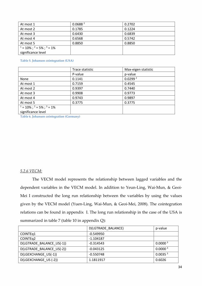
Table 5. Johansen cointegration (USA)

Table 6. Johansen cointegration (Germany)

5.2.6 VECM:

The VECM model represents the relationship between lagged variables and the

dependent variables in the VECM model. In addition to Yeun-Ling, Wai-Mun, & Geoi-

Mei I constructed the long run relationship between the variables by using the values

given by the VECM model (Yuen-Ling, Wai-Mun, & Geoi-Mei, 2008). The cointegration

relations can be found in appendix I. The long run relationship in the case of the USA is

summarized in table 7 (table 10 in appendix Q):

D(LGTRADE_BALANCE) p-value COINTEq1 -0.549950 COINTEq2 -1.104187 D(LGTRADE_BALANCE_US(-1)) -0.314543 0.0000 3 D(LGTRADE_BALANCE_US(-2)) -0.043125 0.0000 3 D(LGEXCHANGE_US(-1)) -0.550748 0.0035 3 D(LGEXCHANGE_US (-2)) 1.1811917 0.6026

At most 1 0.0688 2 0.2702 At most 2 0.1785 0.1224 At most 3 0.6430 0.6839 At most 4 0.6568 0.5742 At most 5 0.8850 0.8850 1 = 10% ; 2 = 5% ; 3 = 1% significance level

Trace statistic Max-eigen statistic P-value p-value None 0.1141 0.0299 2 At most 1 0.7159 0.4545 At most 2 0.9397 0.7440 At most 3 0.9908 0.9773 At most 4 0.9743 0.9897 At most 5 0.3775 0.3775 1 = 10% ; 2 = 5% ; 3 = 1% significance level

34

D(LGGAS_PRICE(-1)) 0.856399 0.7249 D(LGGAS_PRICE(-2)) -0.999308 0.2201 D(LGGDP_RUSSIA(-1)) 0.124807 0.3026 D(LGGDP_RUSSIA(-2)) 0.080271 0.2599 D(LGGDP_US(-1)) -6.054411 0.0401 2 D(LGGDP_US(-2)) -36.58325 0.1773 D(LGOIL_PRICE(-1)) 1.431574 0.8431 D(LGOIL_PRICE(-2)) 1.508229 0.2145 C 0.113650 0.0305 2 1 = 10% ; 2 = 5% ; 3 = 1% significance level Table 7. VECM (USA)

The coefficients in the cointegration equation in appendix I give the estimated

long-run relationship among the variables; the coefficients on that term in the VECM

show how deviations from that long-run relationship affect the changes in the variable in

the next period. As can be seen from table 7 above, there are only a couple of variables

that are significant in the VECM and therefore significantly explain how deviations from

that long-run relationship affect the changes in the variable in the next period ; the first

and second lag of the variable “lgtrade_balance_us”, the first lagged real exchange rate

and the first lag of the variable “lggdp_us”. Since only a few variables in the above

equation are significant at a 5% significance level, the above VECM result should be

interpreted with care.

Same can be said when I look at the VECM of the Germany case. As can be seen

from table 8 below, there are only a couple of variables that are significant in the VECM

and therefore significantly explain how deviations from that long-run relationship affect

the changes in the variable in the next period; The first and second lagged variable

“lgtrade_balance_ger”, the second lagged GDP of Russia and the second lag of the

variable “lggas_price” . The VECM below should also be interpreted with care, since also

here only some variables in the above equation are significant at a 5% significance level.

The long run relationship for the Germany case is given by the following VECM model,

summarized in table 8 (table 11 in appendix Q):

D(LGTRADE_BALANCE) p-value COINTEq1 -0.630306 COINTEq2 -3.846402 D(LGTRADE_BALANCE_GER(-1)) -0.290451 0.0195 2

35

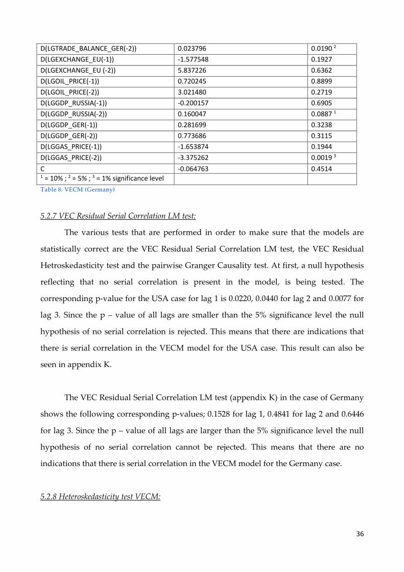
D(LGTRADE_BALANCE_GER(-2)) 0.023796 0.0190 2 D(LGEXCHANGE_EU(-1)) -1.577548 0.1927 D(LGEXCHANGE_EU (-2)) 5.837226 0.6362 D(LGOIL_PRICE(-1)) 0.720245 0.8899 D(LGOIL_PRICE(-2)) 3.021480 0.2719 D(LGGDP_RUSSIA(-1)) -0.200157 0.6905 D(LGGDP_RUSSIA(-2)) 0.160047 0.0887 1 D(LGGDP_GER(-1)) 0.281699 0.3238 D(LGGDP_GER(-2)) 0.773686 0.3115 D(LGGAS_PRICE(-1)) -1.653874 0.1944 D(LGGAS_PRICE(-2)) -3.375262 0.0019 3 C -0.064763 0.4514 1 = 10% ; 2 = 5% ; 3 = 1% significance level Table 8. VECM (Germany)

5.2.7 VEC Residual Serial Correlation LM test:

The various tests that are performed in order to make sure that the models are

statistically correct are the VEC Residual Serial Correlation LM test, the VEC Residual

Hetroskedasticity test and the pairwise Granger Causality test. At first, a null hypothesis

reflecting that no serial correlation is present in the model, is being tested. The

corresponding p-value for the USA case for lag 1 is 0.0220, 0.0440 for lag 2 and 0.0077 for

lag 3. Since the p – value of all lags are smaller than the 5% significance level the null

hypothesis of no serial correlation is rejected. This means that there are indications that

there is serial correlation in the VECM model for the USA case. This result can also be

seen in appendix K.

The VEC Residual Serial Correlation LM test (appendix K) in the case of Germany

shows the following corresponding p-values; 0.1528 for lag 1, 0.4841 for lag 2 and 0.6446

for lag 3. Since the p – value of all lags are larger than the 5% significance level the null

hypothesis of no serial correlation cannot be rejected. This means that there are no

indications that there is serial correlation in the VECM model for the Germany case.

5.2.8 Heteroskedasticity test VECM:

36

The null hypothesis of the hetroskedasticity test is that there is homoskedasticity or no

hetroskedasticity. The p-value of the test is 0.0000 (appendix L) and hence the null

hypothesis is rejected. This is an indication that there is hetroskedasticity in the VECM

model for the USA case.

The p-value of the heteroskedasticity test for the Germany case is 0.3321

(appendix L) and hence we do not reject the null hypothesis. This is an indication that

there is no hetroskedasticity in the VECM model for the Germany case.

5.2.9 Pairwise Granger Causality test:

Results of the Pairwise Granger Causality test are shown in appendix N. The GDP

of the United States does Granger cause the GDP of Russia but not vice versa. The real

exchange rate (Russian Ruble /US$) does not Granger cause the US GDP and the same is

true for the causality between the American GDP and the real exchange rate (Russian

Ruble /US$). The causality between the trade balance of Russia and the US GDP runs

from the US GDP to the trade balance. In other words, the US GDP does Granger cause

the trade balance. This is easy to understand, since the US GDP will always have a effect

on the amount of trade and therefore on the trade balance between the two countries. The

oil price does Granger cause the Russian GDP, but the Russian GDP does not Granger

cause the oil price. The same is true for the gas price; the gas price does Granger cause the

Russian GDP, but the Russian GDP does not Granger cause the gas price. This is really

logical, looking at the fact that the Russian GDP depends a lot on the sale of natural

resources as gas and oil. A change in the prices of these resources has a big effect on the

GDP of Russia. It is therefore not strange that the oil – and gas prices Granger cause the

Russian GDP.

The real exchange rate (Russian Ruble /US$) does not Granger cause the Russian

GDP and the GDP of Russia does not Granger cause the real exchange rate between the

Russian Ruble and the US Dollar. This could be seen as something strange, since Russia

has large oil sales and most of the oil businesses use the US Dollar as currency to price

and buy/sell their oil. You would therefore expect a lot of currency trading between the

37

Russian Ruble and the US Dollar and would therefore expect a causal relationship

between these two variables.

The oil price does not Granger cause the US GDP and same is true vice versa. The

gas price does not Granger cause the US GDP, but the US GDP does Granger cause the

gas price. The most important one for this research, shows no causal relationship

between the real exchange rate (Russian Ruble /US$) and the trade balance between

Russia and the USA.

As can be seen in appendix N, the pairwise Granger Causality tests tell us that the

GDP of Germany does not Granger cause the GDP of Russia, but the GDP of Russia does

Granger cause the GDP of Germany. The real exchange rate (Russian Ruble/EU€) does

Granger cause the Russian GDP, something that can be explained by the huge gas sales of

Russia to European countries. The GDP of Russia does not Granger cause the real

exchange rate between the Russian Ruble and the Euro. The real exchange rate (Russian

Ruble/EU€) does Granger cause the German GDP, but as was the case with the GDP of

Russia, the GDP of Germany does not Granger cause the real exchange rate between the

Russian Ruble and the Euro. There is no causality between the trade balance of Russia

and the German GDP. The oil price does Granger cause the Russian GDP, but the Russian

GDP does not Granger cause the oil price. The same is true for the gas price; the gas price

does Granger cause the Russian GDP, but the Russian GDP does not Granger cause the

gas price. The oil price does not Granger cause the German GDP as is the case vice versa.

The gas price does not Granger cause the German GDP, but the German GDP does

Granger cause the gas price. The most important one for this research, shows no causal

relationship between the real exchange rate (Russian Ruble/EU€) and the trade balance

between Russia and Germany.

5.2.10 Impulse response function:

The response impulse function provides some interesting insights in the effect of

one variable on a other in the short run (instant effect) and the long run (10 months

38

horizon). The response impulse function shows how an increase in one variable behaves

over 10 months in terms of another variable. The influence of the real exchange rate on

the trade balance has our biggest interest (See appendix M for all the impulse response

function graphs). Especially the graphs with the titles “lgtrade_balance_us to

lgexchange_us” and “lgtrade_balance_ger to lgexchange_eu” are interesting. These

graphs can be seen below in figures 4 and 5.

Figure 4. Impulse response graph lgtrade_balance_us to lgexchange_us

Figure 5. Impulse response graph lgtrade_balance_ger to lgexchange_eu

With the use of these graphs I can see if a J-curve exists in our research for Russia.

The graphs do slightly behave in a way that can be expected if there would be a J-curve.

If the real exchange rate increases by one standard deviation, the more costly imports and

less valuable exports lead to a decrease of the trade balance. However, due to the

competitive, relatively low-priced exports, a country's exports start to increase and the

trade balance eventually improves to better levels compared to before the devaluation.

However, after this increase, it decreases again. In the case of a J-curve, I would have

expected an instant decrease of the trade balance the moment the real exchange rate

39

increased and a improvement of the trade balance till a level higher than the level of the

trade balance before the depreciation rate after that, but there wouldn’t be a decrease

after this. Since this is the case in both figures, I have to conclude that the impulse

response functions do not really support the J-curve in my research.

The previous research showed some interesting results. With the use of unit root tests I

showed that all the variables that are used in this thesis are stationary when taking the

first differences. The Engle Granger cointegration approach showed that for Germany

there is a unit root, the residual term isn’t stationary and the variables are not

cointegrated. This is different for the USA, for which there is no unit root, the residual

term is stationary and all variables are cointegrated. The different types of Johansen

cointegration tests showed some different results to. The trace tests indicate that there are

2 cointegration relationships for the USA and 0 cointegration relationships when we look

at Germany. The eigenvalue tests show something different, indicating that there are no

cointegration relationships for the USA and 1 cointegration relationship for Germany.

The VEC residual serial correlation LM test showed that there are indications of serial

correlation in the USA VEC model. The Germany VEC model had no indications of serial

correlation. The heteroskedasticity tests also showed some opposing results, indicating

that there is heterskedasticity in the USA VEC model, but no heterskedasicity in the

Germany VEC model. The most important result of this research is that the impulse

response functions do not really support the J-curve in my research.

40

6. Conclusion:

Goldman Sachs published a research paper in 2002 about potential economic

superpowers of the 21th century (Cooper, 2009). Based on this study, Russia was seen

by many as an emerging superpower economy and one of the most dominant

economies to be in the middle of the current century.

Russia experienced some impressive economic growth, with real gross domestic

product increasing 6.9% annually on average, which helped to raise the Russian standard

of living and brought economic stability (Cooper, 2009). The crisis in the last quarter of

2008 brought an abrupt end to this period of growth. The Russian economy was, like

many other economies, hit substantially by the global financial crisis. The unavoidable

outcome of this all for Russia: Recession! (Cooper, 2009). In dealing with the

consequences of this crisis, Russia also had to make some important decisions regarding

its exchange rate policy.

Russia caught my attention as this big economic power had to deal with many political

and economic changes in the past. The change came in many (positive/negative) flavors

and had various impacts on the Russian economy and the well-being of the Russian

population. By learning from the past, I hoped to be able to predict the future better. I

formulated the main question:

How will the currency policy of Russia impact the international trade position of the country and

what do we predict to happen with the future bilateral trade between Russia, Germany and the

USA?

The conducted literature review already visualized the difficulty to find relevant

relationships between economic variables that would allow good forecasting. A rare

exception to above was the linkage of “exchange rate” variable and the “net-trade”

variable for a few cases.

41

Additional sub-questions were formulated and started the focus on Russia:

1 = How did the exchange rate policy of Russia develop over the years?

2= How did Russia’s economic situation evolve over the years?

3 = What do we predict to happen with the future bilateral trade between Russia, Germany and

the USA?

The first sub question showed that Russia has had quite some changes in its

exchange rate system during the years. In 1995, Russia had an exchange rate corridor

system, strengthening the role of the ruble exchange rate as the nominal policy anchor.

Since 1999, the Bank of Russia implemented a policy of a managed floating exchange rate,

which contributed to the smoothening of the influence of changes in external conditions

on the Russian financial markets and the Russian economy as a whole. In 2005, the Bank

of Russia introduced a dual-currency basket as the operational indicator for its exchange

rate policy. Again, the aim was to smoothen the volatility of the ruble’s exchange rate in

relation to other major currencies. During the period of November 2008 to January 2009,

the Bank of Russia allowed the ruble to depreciate gradually by widening the dual-

currency band and in January 2009, the Bank of Russia announced a wide fixed band for

the ruble value of the dual-currency basket (allowing fluctuations from 26 to 41 rubles)

and it also introduced a floating operational band. During 2009–2012, the Bank of Russia

further increased the flexibility of its exchange rate policy; the floating operational band

was widened from 2 to 7 rubles and from November 2014 on, the Bank of Russia finally

abolished the exchange rate policy mechanism through cancelling the range of the dual-

currency basket ruble values and regular interventions on and outside the borders of this

band.

42

The second sub question showed that the Russian economy and the Russian

economic situation changed significantly over the years. Russia started with economic

problems around the time of the financial crisis (August 1998). The world-wide financial

crisis was a clear trigger point in Russia to start with the implementation of economic

reforms as shortcomings in the existing economic policies had to be addressed. Off course

many of these policies had their roots in the communist history of the country in which

industrial production was seen as the crucial corner stone of economic success. This

specific focus made other sectors (services, consumer industry, food/agriculture) suffer.

This shortcoming could well be compensated during economic growth as import of

“goods needed” was relatively easy. Standards of living did rise constantly and resulted

in great political and economic stability in the country.

The 2008 crisis brought an abrupt end to this period. The Russian economy was,

like other economies, hit substantially by the global financial crisis. The economic success

of Russia was mainly based on high oil prices, but when the prices of both oil and other

commodities went down in 2008, the Russian economy suffered heavily. Both production

and, even more importantly, export of oil and gas went down rapidly (Cooper, 2009). The

unavoidable outcome of this all for Russia: Recession (Cooper, 2009)!

Sub question three showed a low significance of the relations in the three

forecasting models. The models were not progressed any further as results would not be

valuable.

The standard OLS regression shows that an appreciation of the exchange rate

(Russian Ruble /US$) is followed by an decrease in the trade balance between Russia and

the USA. An decrease in the trade balance means that the exports decrease relative to the

imports. This also means that if the real exchange rate appreciates, the trade balance

increases as well, meaning that the amount of imports decreases relatively to the amount

of exports. This is in contrast with standard economic intuition but can be seen as (weak)

43

support for the J-curve, which says that the trade balance is worse off in the short run

after a depreciation of the real exchange rate and improves in later periods.

From the Engle Granger cointegration approach we can conclude that for the USA

case, the variables are cointegrated and that a long run relationship between the variables

therefore exists. For the Germany case we can conclude that there is a unit root, that the

residual term is not stationary and that the variables are not cointegrated and that there

therefore doesn’t exist a long run relationship between the variables.

The VEC model, which also captures the long run relationship between the

variables, does not provide evidence that the real exchange rate has a significant effect on

the trade balance. Also the pairwise Granger causality test does not support the causal

relationship between the real exchange rate or the trade balance.

The main figure for our analysis about the relationship between the real exchange

rate (Russian Ruble /US$ and Russian Ruble/EU€) and the trade balance (with

Germany/the USA) is the impulse response function. This function shows the moment

the real exchange rate moves and the effect it has on the trade balance of Russia. The

graphs do slightly behave in a way that can be expected if there would be a j-curve. If the

real exchange rate increases by one standard deviation, the trade balance first decreases

and then increases to a point that is slightly higher than the starting point. But finally it

decreases again. In the case of a J-curve, I would have expected an instant decrease of the

trade balance if the real exchange rate increased and later on an improvement of the trade

balance to a level higher than the level of the trade balance before the depreciation of the

real exchange rate. There shouldn’t be a decrease after this. Therefore I have to conclude

that the impulse response function does not really support the J-curve in our research.

44

Final conclusion: There is no doubt of the fact that Russia is one of the current and

“to be” economic powers. It is the obligation of the Russian government to use all macro-

economic possibilities to stimulate the growth of their economy. Of course cannot all

factors, of which some external, be handled easily and quite a few of those factors are

unpredictable. In this environment using forecasting modeling to predict bilateral trade

volumes between Russia and Germany and the USA, proofed to be impossible. Detailed

analysis in this master Thesis re-confirmed this with supporting data.

45

7. Bibliography:

Akbostanci, E. (2002). Dynamics of the Trade Balance: The Turkish J-Curve. Ankara:

Department of Economics.

Backus, D. (1986). The Canadian--U.S. Exchange Rate: Evidence from a Vector Autoregression. The Review of Economics and Statistics , 628-637.

Bahmani - Oskooee, M. (2001). Nominal and real effective exchange rates of middle eastern countries and their trade performance. Applied Economics , 103-111.

Bahmani-Oskooee, M., & Brooks, T. (1991). Bilateral J-Curve between U.S. and her trading partners. Review of World Economics , 156-165.

Brugato, T. (2008). Drunk On Oil: Russian Foreign Policy 2000-2007. Berkley Undergraduate Journal .

Central Bank of Russia. (2014, November 13). The History of the Bank of Russia FX policy in 1999 — 2010 years. Retrieved February 12, 2015, from The Bank of Russia FX policy : http://www.cbr.ru/eng/dkp/?PrtId=e-r_policy

Central Bank of the Russian Federation. (2014). The history of the Bank of Russia’s exchange rate. BIS Paper volume 73 , 293-299.

Cooper, W. H. (2009). Russia’s Economic Performance and Policies and Their Implications for the United States. Congressional Research Service.

Dickey, D. A., & Fuller, W. A. (1981). likelihood ratio statistics for autoregressive time series with a unit root. Econometrica , 1057.

Edwards, S. (2001). Exchange rate regimes, capital flows and crisis prevention. Cambridge: National Bureau of Economic Research.

Engle, R. F., & Granger, C. W. (1992). Long-Run Economic Relationships. Oxford University Press.

Gaddy, C. G., & Ickes, B. W. (2010). Russia after the Global Financial Crisis. Eurasian Geography and Economics , 281-311.

Hashim, I., & Zarma, A. (1996). The Impact of Parallel Market on the Stability of Exchange Rate: Evidence from Nigeria. NDIC Quarterly .

Hoeven, J. v. (2013). What effects does the currency policy of Brazil have on the international trade position of the country and what do we expect to happen with the net

46

trade between Brazil and the USA in the future? Rotterdam: Erasmus University Rotterdam.

Johansen, S. (1988). Statistical analysis of cointegration vectors. Journal of Economic Dynamics and Control , 231-254.

Kale, P. (2001). Turkey's Trade Balance in the short and long run: Error Correction Modeling and Cointegration. International Trade Journal , 27-55.

Kuboniwa, M. (2010). Diagnosing the ‘Russian Disease’: Growth and Structure of the Russian Economy. Tokyo: The Institute of Economic Research.

Liew, K.-S., Lim, K.-P., & Hussain, H. (2003). Exchange Rate and Trade Balance Relationship: The Experience of ASEAN Countries.

Liu, L.-g., Fan, K., & Shek, J. (2007). Hong Kong's Trade Patterns and Trade Elasticities. Hong Kong Monetary Authority Quaterly Bulletin , 21-31.

MacKinnon, J. G. (2010). Critical Values for Cointegration Tests. Ontario: Department of Economics.

Moffett, M. H. (1989). The J-Curve revisited: an empirical examination for the United States . Journal of International Money and Finance , 425-444.

Onafowora, O. (2003). Exchange rate and trade balance in east asia: is there a J−curve? Economic Bulletin , 1-13.

Pesaran, M., Shin, Y., & Smith, R. (1996). Testing for the 'Existence of a Long-run Relationship'. Cambridge Working Papers in Economics .

Purushothaman, R., & Wilson, D. (2003). Dreaming With BRICs: The Path to 2050. The Goldman Sachs Group.

Rautava, J. (2004). The role of oil prices and the real exchange. Journal of Comparative Economics.

Rey, H. (2001). International Trade and Currency exchange. Oxfor University Press.

Rose, A. K. (1991). The role of exchange rates in a popular model of international trade: Does the 'Marshall-Lerner' condition hold? Journal of International Economics , 301-316.

Rose, A., & Yellen, J. (1989). Is there a J-curve? Journal of Monetary Economics , 53-68.

Sachs, J. D. (1996). Economic Transition and the Exchange-Rate Regime. The American Economic Review , 147-152.

47

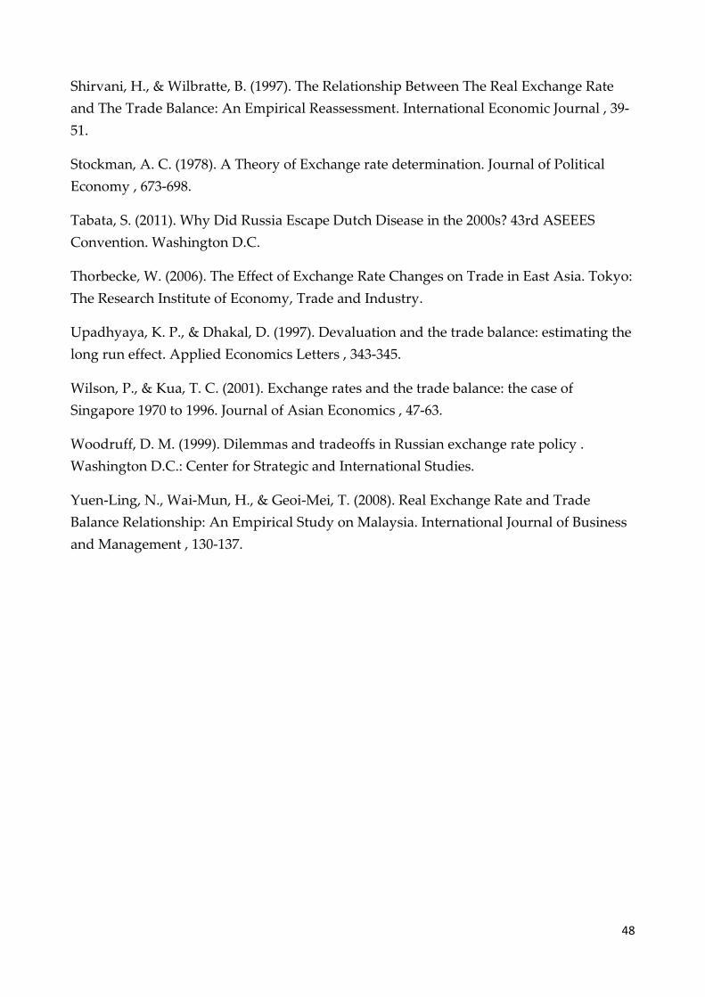
Shirvani, H., & Wilbratte, B. (1997). The Relationship Between The Real Exchange Rate and The Trade Balance: An Empirical Reassessment. International Economic Journal , 39-51.

Stockman, A. C. (1978). A Theory of Exchange rate determination. Journal of Political Economy , 673-698.

Tabata, S. (2011). Why Did Russia Escape Dutch Disease in the 2000s? 43rd ASEEES Convention. Washington D.C.

Thorbecke, W. (2006). The Effect of Exchange Rate Changes on Trade in East Asia. Tokyo: The Research Institute of Economy, Trade and Industry.

Upadhyaya, K. P., & Dhakal, D. (1997). Devaluation and the trade balance: estimating the long run effect. Applied Economics Letters , 343-345.

Wilson, P., & Kua, T. C. (2001). Exchange rates and the trade balance: the case of Singapore 1970 to 1996. Journal of Asian Economics , 47-63.

Woodruff, D. M. (1999). Dilemmas and tradeoffs in Russian exchange rate policy . Washington D.C.: Center for Strategic and International Studies.

Yuen-Ling, N., Wai-Mun, H., & Geoi-Mei, T. (2008). Real Exchange Rate and Trade Balance Relationship: An Empirical Study on Malaysia. International Journal of Business and Management , 130-137.

48

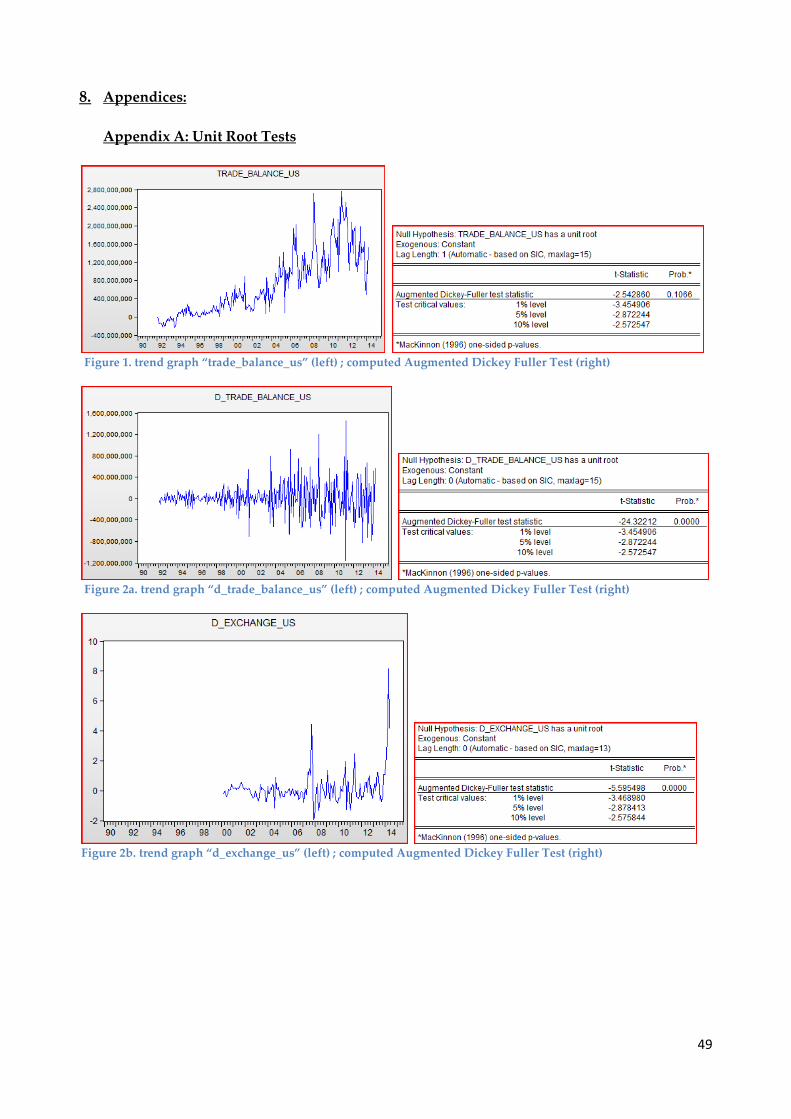
8. Appendices: Appendix A: Unit Root Tests

Figure 1. trend graph “trade_balance_us” (left) ; computed Augmented Dickey Fuller Test (right)

Figure 2a. trend graph “d_trade_balance_us” (left) ; computed Augmented Dickey Fuller Test (right)

Figure 2b. trend graph “d_exchange_us” (left) ; computed Augmented Dickey Fuller Test (right)

49

Figure 2c. trend graph “d_gdp_us” (left) ; computed Augmented Dickey Fuller Test (right)

Figure 2d. trend graph “d_gdp_russia” (left) ; computed Augmented Dickey Fuller Test (right)

Figure 2e. trend graph “d_oil_price” (left) ; computed Augmented Dickey Fuller Test (right)

Figure 2f. trend graph “d_gas_price” (left) ; computed Augmented Dickey Fuller Test (right)

50

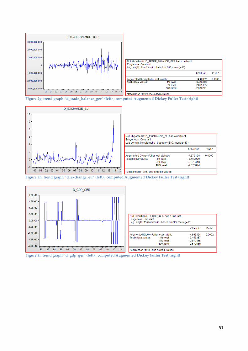
Figure 2g. trend graph “d_trade_balance_ger” (left) ; computed Augmented Dickey Fuller Test (right)

Figure 2h. trend graph “d_exchange_eu” (left) ; computed Augmented Dickey Fuller Test (right)

Figure 2i. trend graph “d_gdp_ger” (left) ; computed Augmented Dickey Fuller Test (right)

51

Appendix B: Serial Correlation Tests Correlation test, Normality test, Homoskedasticity test and Linearity test between variables:

Figure 3a. Serial correlation test (left) ; normality test (right) both between “d_trade_balance_us” and “d_exchange_us”.

Figure 3b. Heteroskedasticity test (left) ; linearity test (right) both between “d_trade_balance_us” and “d_exchange_us”.

52

Figure 3c. Serial correlation test (left) ; normality test (right) both between “d_trade_balance_us” and “d_gdp_us”.

Figure 3d. Heteroskedasticity test (left) ; linearity test (right) both between “d_trade_balance_us” and “d_gdp_us”.

53

Figure 3e. Serial correlation test (left) ; normality test (right) both between “d_trade_balance_us” and “d_gdp_russia”.

Figure 3f. Heteroskedasticity test (left) ; linearity test (right) both between “d_trade_balance_us” and “d_gdp_russia”.

54

Figure 3g. Serial correlation test (left) ; normality test (right) both between “d_trade_balance_us” and “d_oil_price”.

Figure 3h. Heteroskedasticity test (left) ; linearity test (right) both between “d_trade_balance_us” and “d_oil_price”.

55

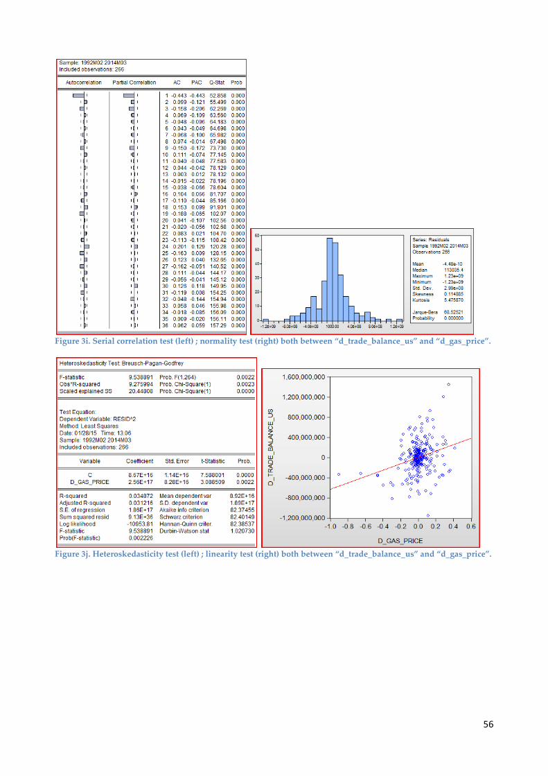
Figure 3i. Serial correlation test (left) ; normality test (right) both between “d_trade_balance_us” and “d_gas_price”.

Figure 3j. Heteroskedasticity test (left) ; linearity test (right) both between “d_trade_balance_us” and “d_gas_price”.

56

Figure 3k. Serial correlation test (left) ; normality test (right) both between “d_trade_balance_ger” and “d_exchange_eu”.

Figure 3l. Heteroskedasticity test (left) ; linearity test (right) both between “d_trade_balance_ger” and “d_exchange_eu”.

57

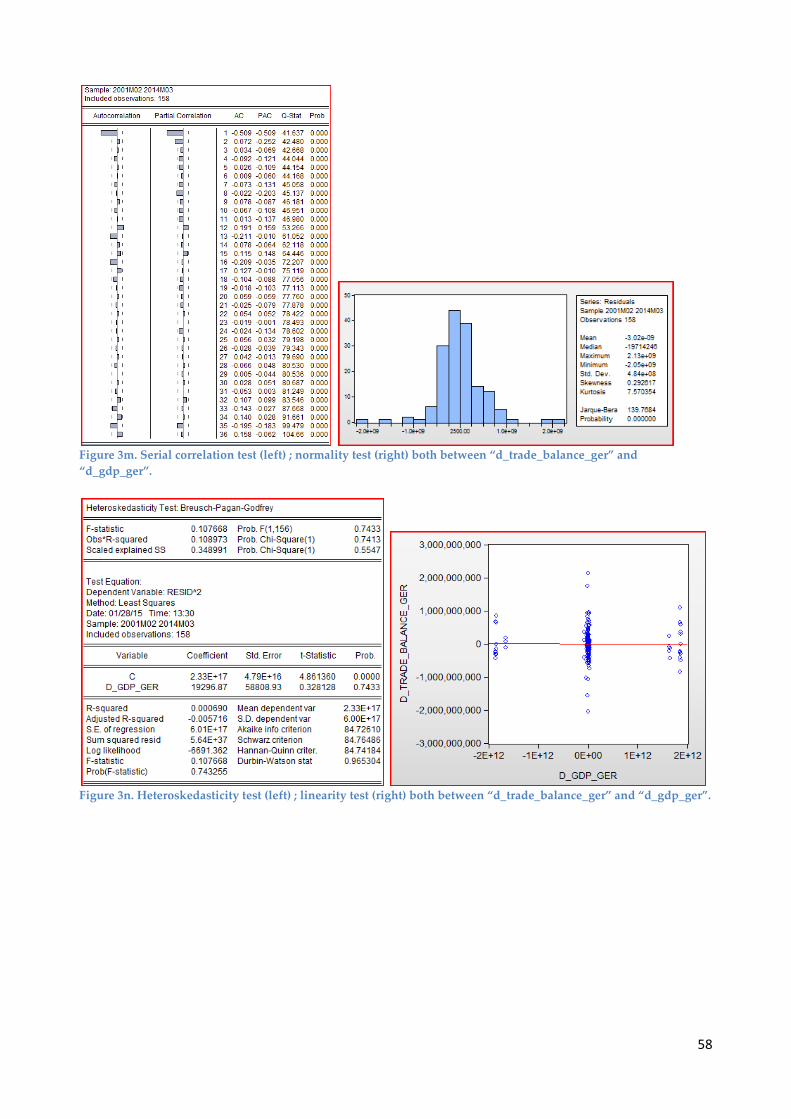
Figure 3m. Serial correlation test (left) ; normality test (right) both between “d_trade_balance_ger” and “d_gdp_ger”.

Figure 3n. Heteroskedasticity test (left) ; linearity test (right) both between “d_trade_balance_ger” and “d_gdp_ger”.

58

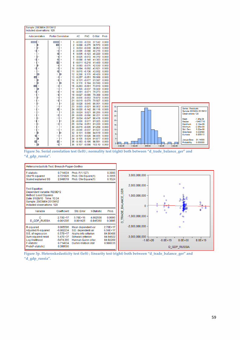
Figure 3o. Serial correlation test (left) ; normality test (right) both between “d_trade_balance_ger” and “d_gdp_russia”.

Figure 3p. Heteroskedasticity test (left) ; linearity test (right) both between “d_trade_balance_ger” and “d_gdp_russia”.

59

Figure 3q. Serial correlation test (left) ; normality test (right) both between “d_trade_balance_ger” and “d_oil_price”.

Figure 3r. Heteroskedasticity test (left) ; linearity test (right) both between “d_trade_balance_ger” and “d_oil_price”.

60

Figure 3s. Serial correlation test (left) ; normality test (right) both between “d_trade_balance_ger” and “d_gas_price”.

Figure 3t. Heteroskedasticity test (left) ; linearity test (right) both between “d_trade_balance_ger” and “d_gas_price”.

61

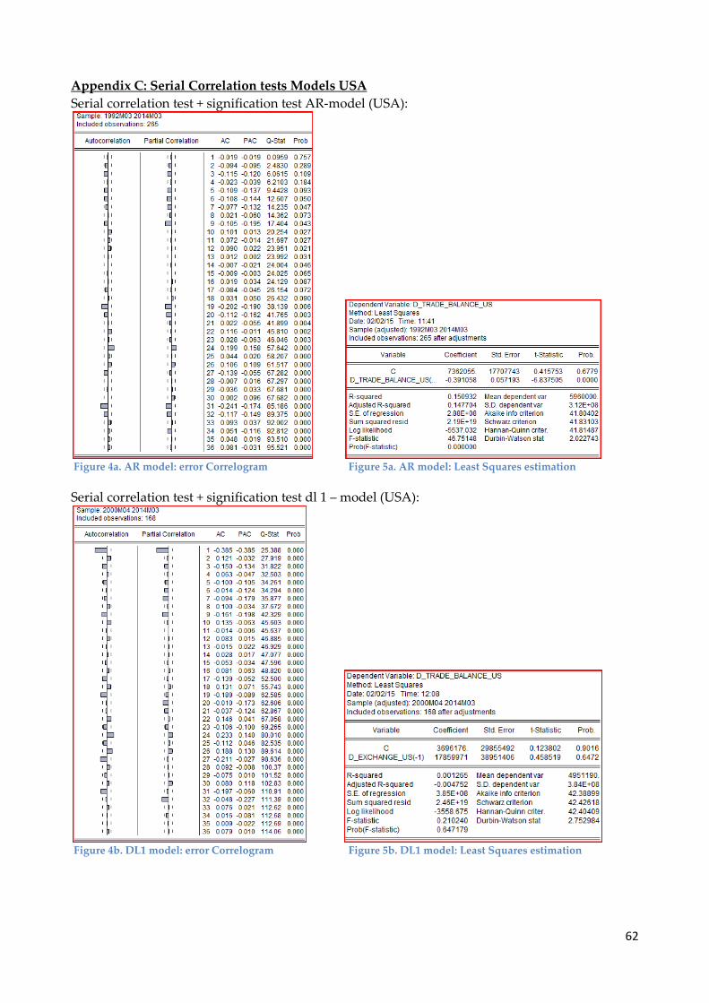
Appendix C: Serial Correlation tests Models USA Serial correlation test + signification test AR-model (USA):

Figure 4a. AR model: error Correlogram Figure 5a. AR model: Least Squares estimation Serial correlation test + signification test dl 1 – model (USA):

Figure 4b. DL1 model: error Correlogram Figure 5b. DL1 model: Least Squares estimation

62

Serial correlation test + signification test dl 2 – model (USA):

Figure 4c. DL2 model: error Correlogram Figure 5c. DL2 model: Least Squares estimation Serial correlation test + signification test dl 3 – model (USA):

Figure 4d. DL3 model: error Correlogram Figure 5d. DL3 model: Least Squares estimation

63

Serial correlation test + signification test dl 4 – model (USA):

Figure 4e. DL4 model: error Correlogram Figure 5e. DL4 model: Least Squares estimation Serial correlation test + signification test ARDL 1 model (USA):

Figure 4f. ARDL1 model: error Correlogram Figure 5f. ARDL1 model: Least Squares estimation

64

Serial correlation test + signification test ARDL 2 model (USA):

Figure 4g. ARDL2 model: error Correlogram Figure 5g. ARDL2 model: Least Squares estimation Serial correlation test + signification test ARDL 3 model (USA):

Figure 4h. ARDL3 model: error Correlogram Figure 5h. ARDL3 model: Least Squares estimation

65

Serial correlation test + signification test ARDL 4 model (USA):

Figure 4i. ARDL4 model: error Correlogram Figure 5i. ARDL4 model: Least Squares estimation Appendix D: Serial Correlation tests Models Germany Serial correlation test + signification test AR-model (GER):

Figure 4j. AR model: error Correlogram Figure 5j. AR model: Least Squares estimation

66

Serial correlation test + signification test dl 1 – model (GER):

Figure 4k. DL1 model: error Correlogram Figure 5k. DL1 model: Least Squares estimation Serial correlation test + signification test dl 2 – model (GER):

Figure 4l. DL2 model: error Correlogram Figure 5l. DL2 model: Least Squares estimation

67

Serial correlation test + signification test dl 3 – model (GER):

Figure 4m. DL3 model: error Correlogram Figure 5m. DL3 model: Least Squares estimation Serial correlation test + signification test dl 4 – model (GER):

Figure 4n. DL4 model: error Correlogram Figure 5n. DL4 model: Least Squares estimation

68

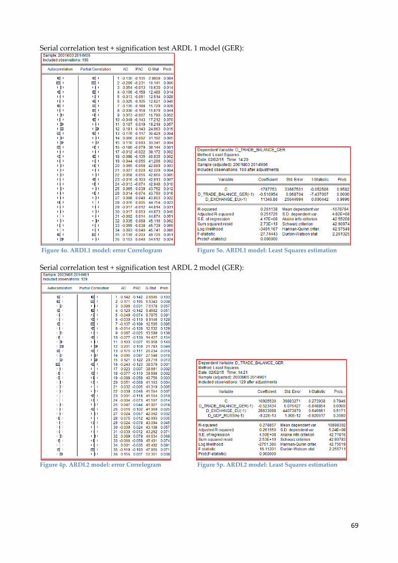
Serial correlation test + signification test ARDL 1 model (GER):

Figure 4o. ARDL1 model: error Correlogram Figure 5o. ARDL1 model: Least Squares estimation Serial correlation test + signification test ARDL 2 model (GER):

Figure 4p. ARDL2 model: error Correlogram Figure 5p. ARDL2 model: Least Squares estimation

69

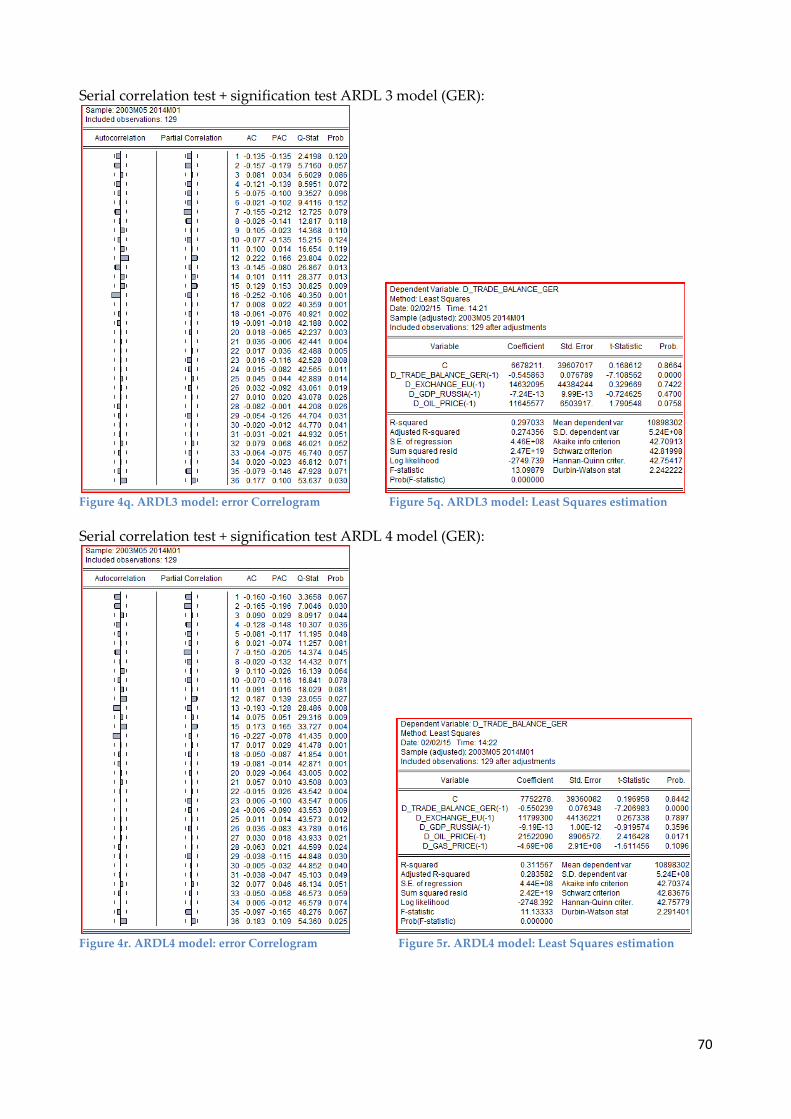
Serial correlation test + signification test ARDL 3 model (GER):

Figure 4q. ARDL3 model: error Correlogram Figure 5q. ARDL3 model: Least Squares estimation Serial correlation test + signification test ARDL 4 model (GER):

Figure 4r. ARDL4 model: error Correlogram Figure 5r. ARDL4 model: Least Squares estimation

70

Appendix E: Trade Balance Regressions

Figure 6.

Figure 7.

71

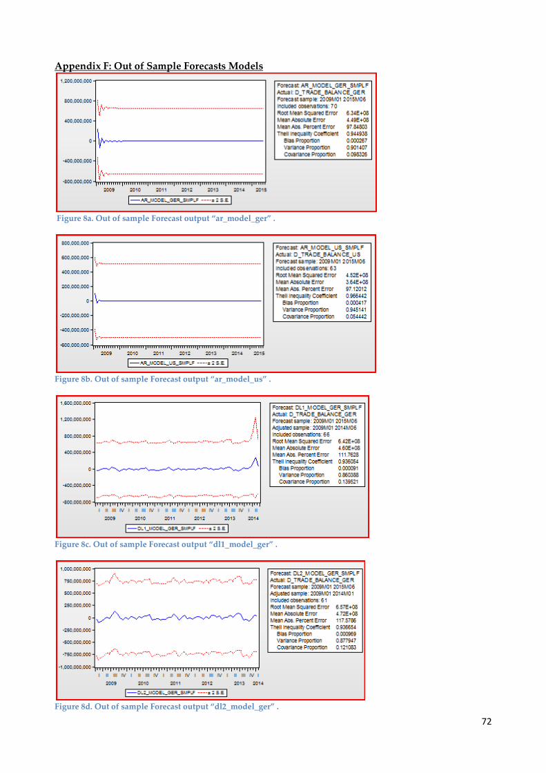
Appendix F: Out of Sample Forecasts Models

Figure 8a. Out of sample Forecast output “ar_model_ger” .

Figure 8b. Out of sample Forecast output “ar_model_us” .

Figure 8c. Out of sample Forecast output “dl1_model_ger” .

Figure 8d. Out of sample Forecast output “dl2_model_ger” .

72

Figure 8e. Out of sample Forecast output “dl3_model_ger” .

Figure 8f. Out of sample Forecast output “dl4_model_ger” .

Figure 8g. Out of sample Forecast output “dl1_model_us” .

Figure 8h. Out of sample Forecast output “dl2_model_us” .

73

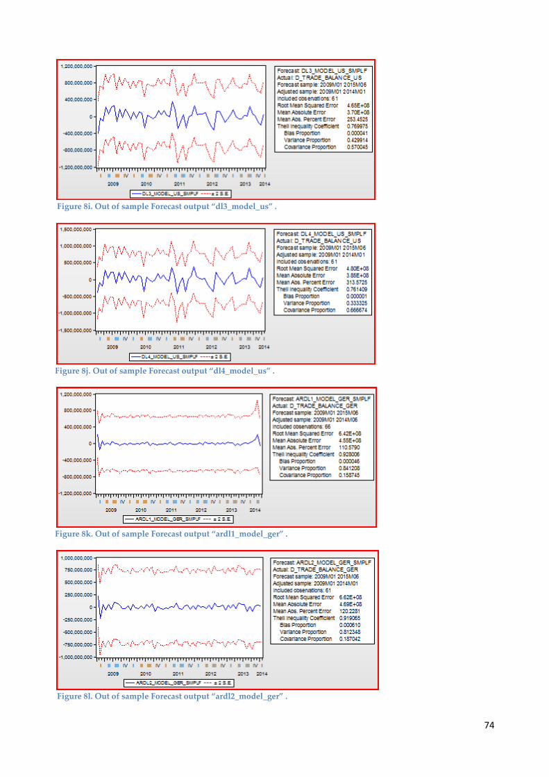
Figure 8i. Out of sample Forecast output “dl3_model_us” .

Figure 8j. Out of sample Forecast output “dl4_model_us” .

Figure 8k. Out of sample Forecast output “ardl1_model_ger” .

Figure 8l. Out of sample Forecast output “ardl2_model_ger” .

74

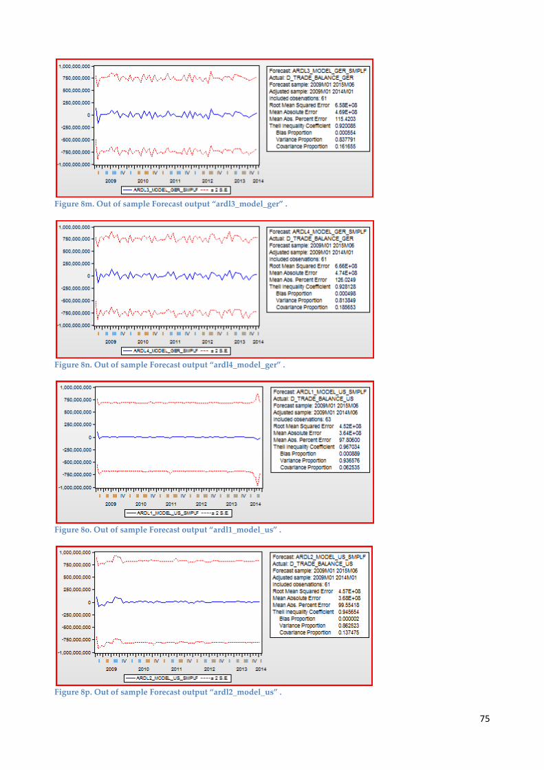
Figure 8m. Out of sample Forecast output “ardl3_model_ger” .

Figure 8n. Out of sample Forecast output “ardl4_model_ger” .

Figure 8o. Out of sample Forecast output “ardl1_model_us” .

Figure 8p. Out of sample Forecast output “ardl2_model_us” .

75

Figure 8q. Out of sample Forecast output “ardl3_model_us” .

Figure 8r. Out of sample Forecast output “ardl4_model_us” .

76

Appendix G: Seemingly Unrelated Regression (SUR)

Figure 9. Seemingly Unrelated Regression (SUR).

77

Appendix H: Johansen Cointegration Tests

78

79

80

Figure 10. Johansen Cointegration Test (USA)

81

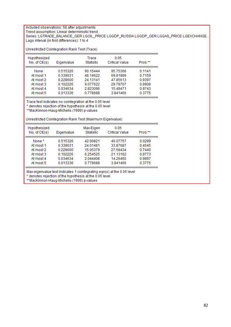
82

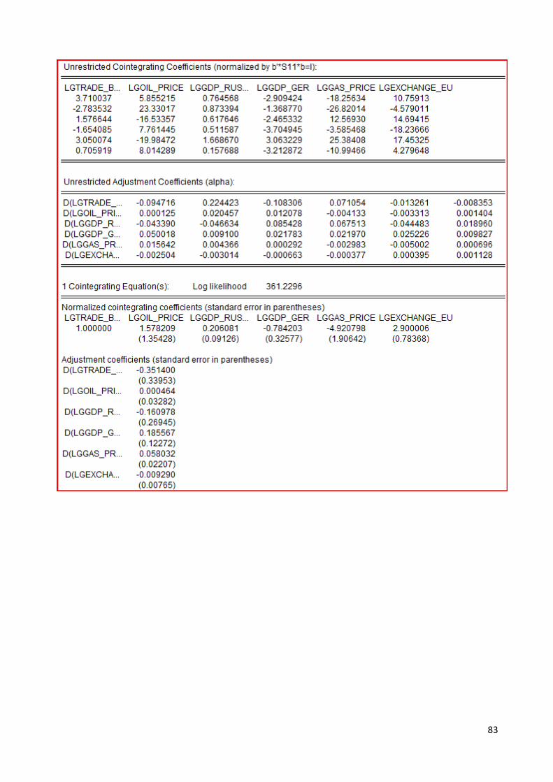
83

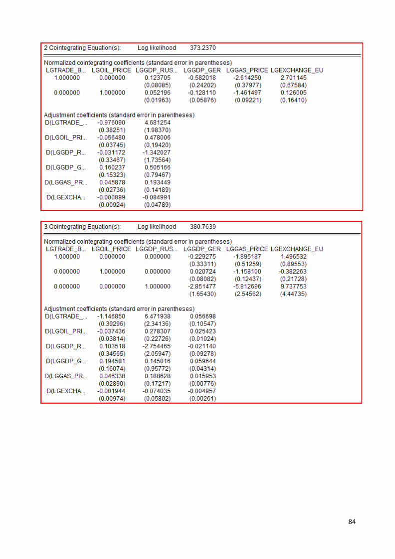
84

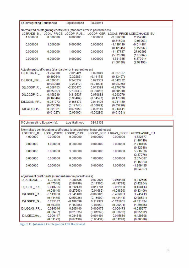
Figure 11. Johansen Cointegration Test (Germany)

85

Appendix I: Vector Error Correction Estimates

86

87

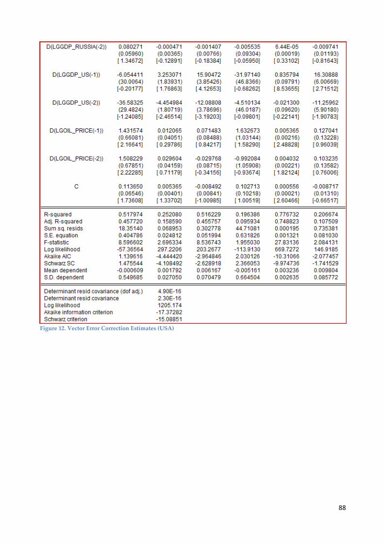
Figure 12. Vector Error Correction Estimates (USA)

88

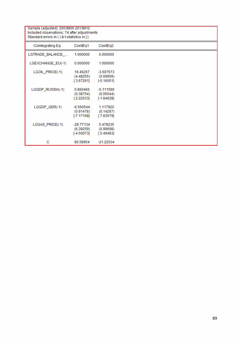
89

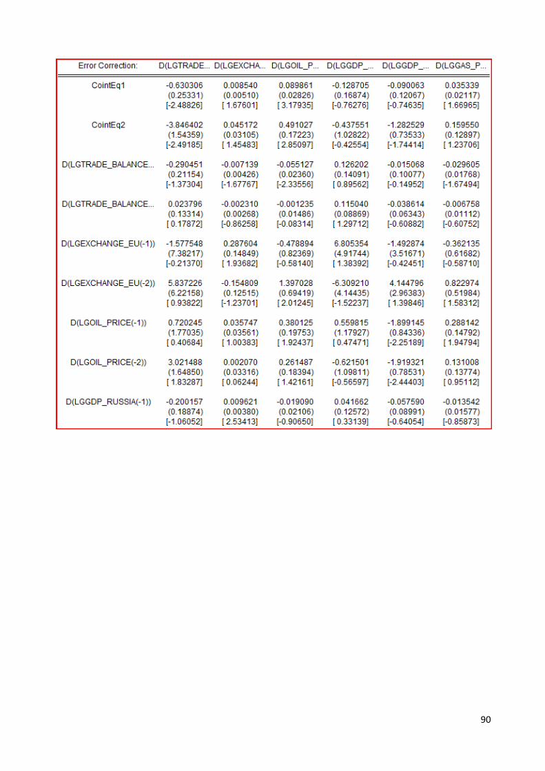
90

Figure 13. Vector Error Correction Estimates (Germany)

91

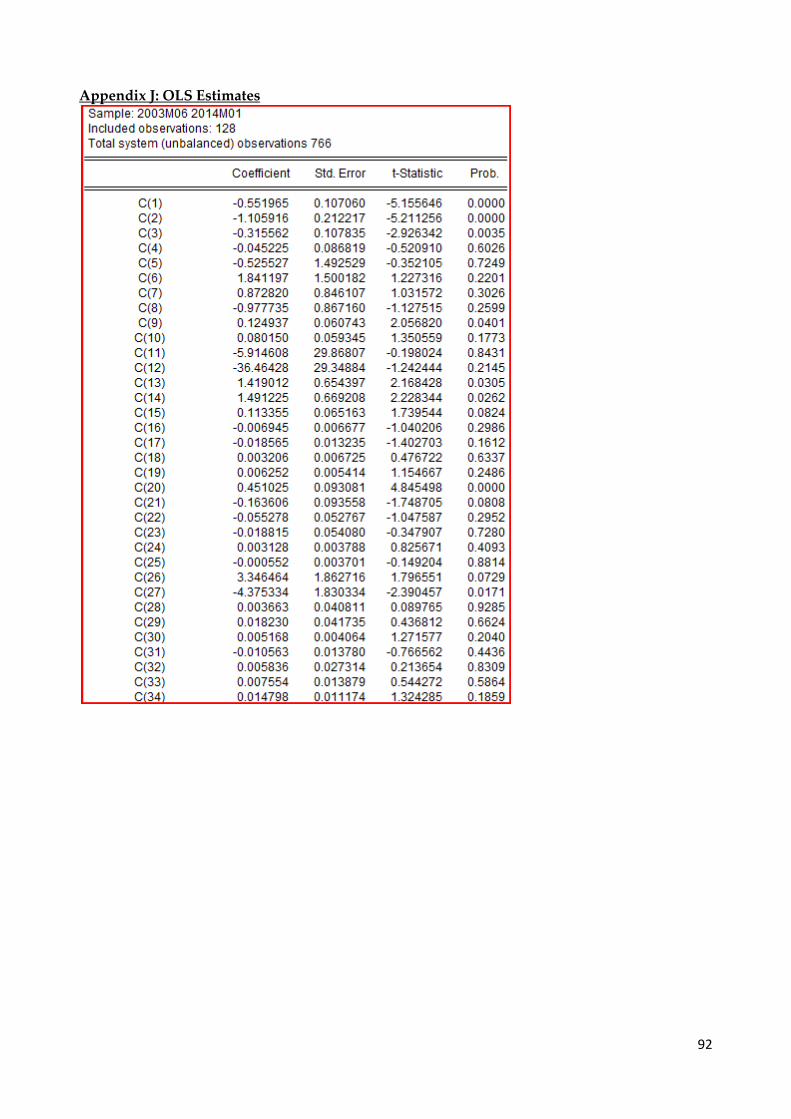
Appendix J: OLS Estimates

92

Figure 14. OLS Estimate (USA)

93

94

Figure 15. OLS Estimate (Germany)

95

Appendix K: LM tests VECM

Figure 16. LM test VECM (USA)

Figure 17. LM test VECM (Germany) Appendix L: Heteroskedasticity Test VECM

Figure 18. Heteroskedasticity Test VECM (USA)

96

Figure 19. Heteroskedasticity Test VECM (Germany)

97

Appendix M: Impulse Graphs

98

Figure 20. Impulse graphs (USA)

99

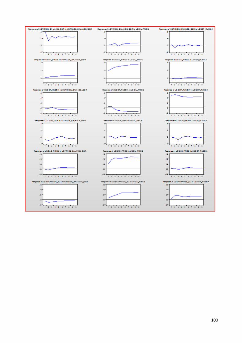
100

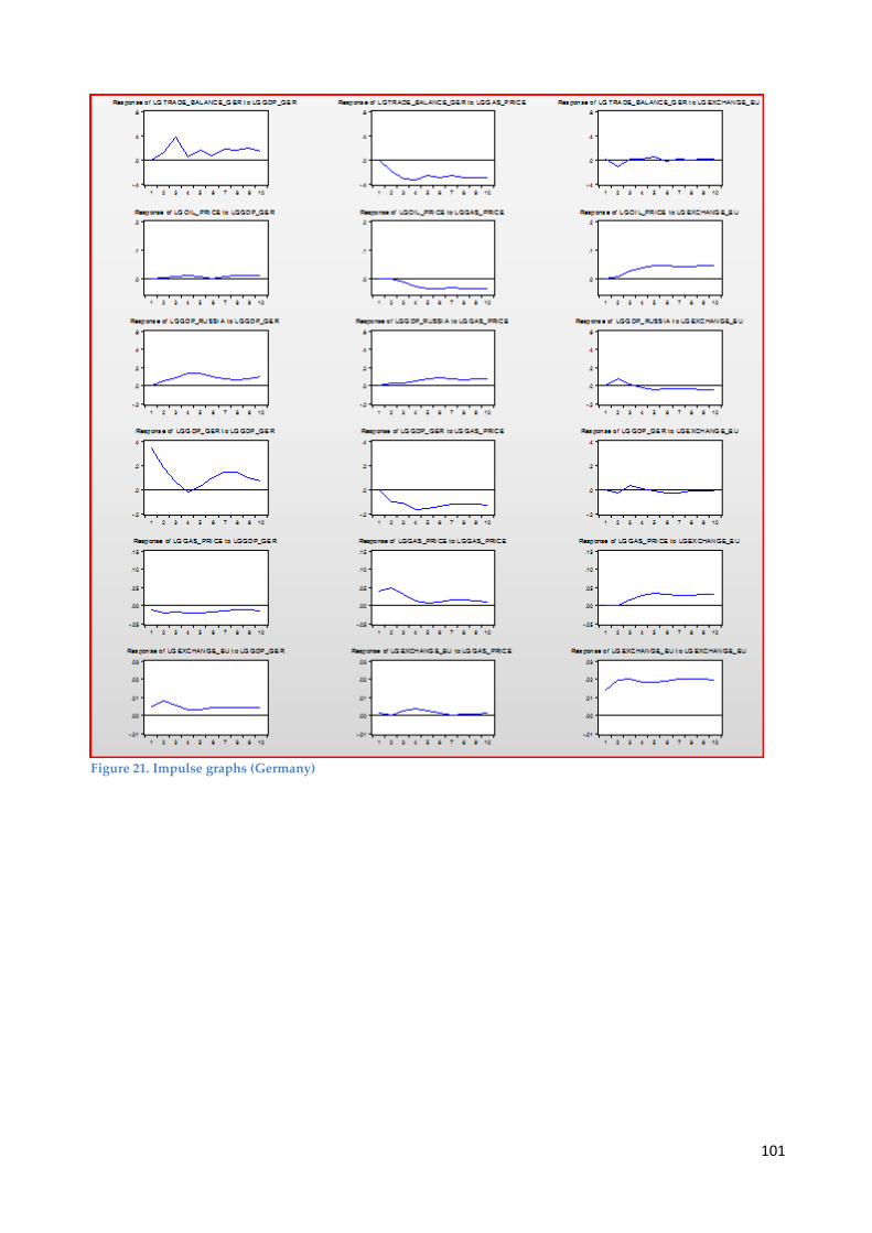
Figure 21. Impulse graphs (Germany)

101

Appendix N: Pairwise Granger Causality Tests

Figure 22. Pairwise Granger Causality Tests (USA)

102

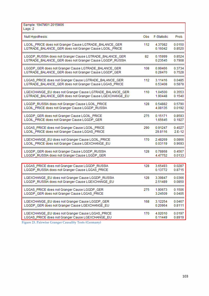
Figure 23. Pairwise Granger Causality Tests (Germany)

103

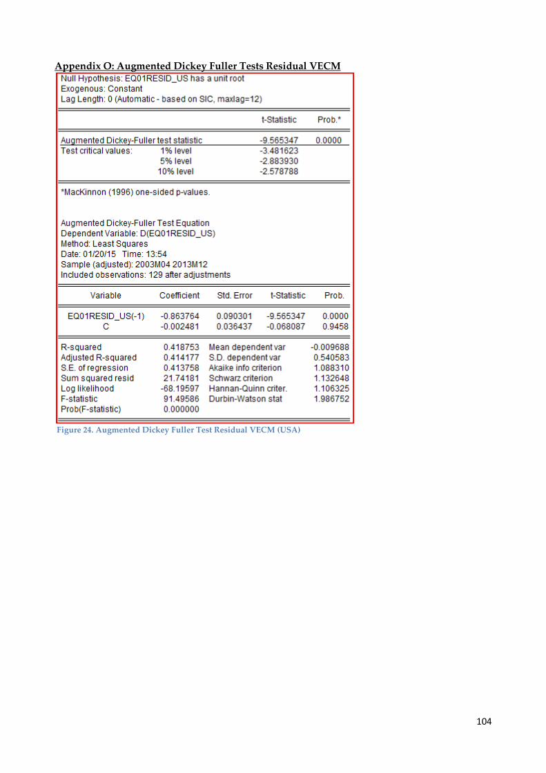
Appendix O: Augmented Dickey Fuller Tests Residual VECM

Figure 24. Augmented Dickey Fuller Test Residual VECM (USA)

104

Figure 25. Augmented Dickey Fuller Test Residual VECM (Germany)

105

Figure 26. OLS output first differences (USA) Appendix P: Augmented Dickey Fuller Unit Root Tests and Philips Perron Unit Root Tests

Augmented Dickey Fuller Unit root test variable lggdp_russia (left: constant ; right: constant + trend)

106

Augmented Dickey Fuller Unit root test variable d_lggdp_russia (left: constant ; right: constant + trend)

Philips Perron Unit root test variable lggdp_russia (left: constant ; right: constant + trend).

107

Philips Perron Unit root test variable d_lggdp_russia (left: constant ; right: constant + trend).

Augmented Dickey Fuller Unit root test variable lggdp_us (left: constant ; right: constant + trend)

108

Augmented Dickey Fuller Unit root test variable d_lggdp_us (left: constant ; right: constant + trend)

Philips Perron Unit root test variable lggdp_us (left: constant ; right: constant + trend).

109

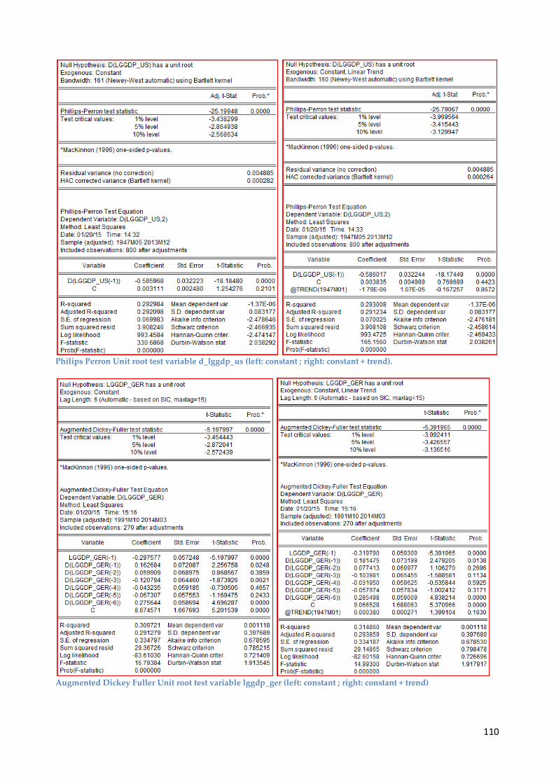
Philips Perron Unit root test variable d_lggdp_us (left: constant ; right: constant + trend).

Augmented Dickey Fuller Unit root test variable lggdp_ger (left: constant ; right: constant + trend)

110

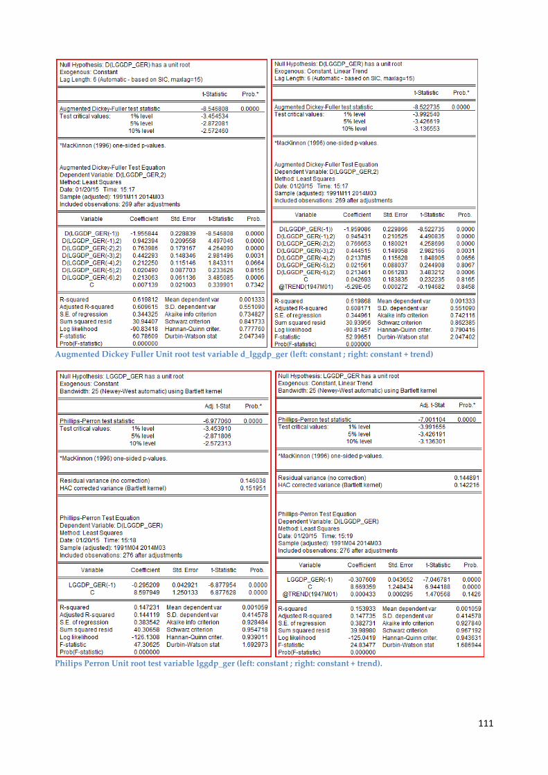
Augmented Dickey Fuller Unit root test variable d_lggdp_ger (left: constant ; right: constant + trend)

Philips Perron Unit root test variable lggdp_ger (left: constant ; right: constant + trend).

111

Philips Perron Unit root test variable d_lggdp_ger (left: constant ; right: constant + trend).

Augmented Dickey Fuller Unit root test variable lgexchange_us (left: constant ; right: constant + trend)

112

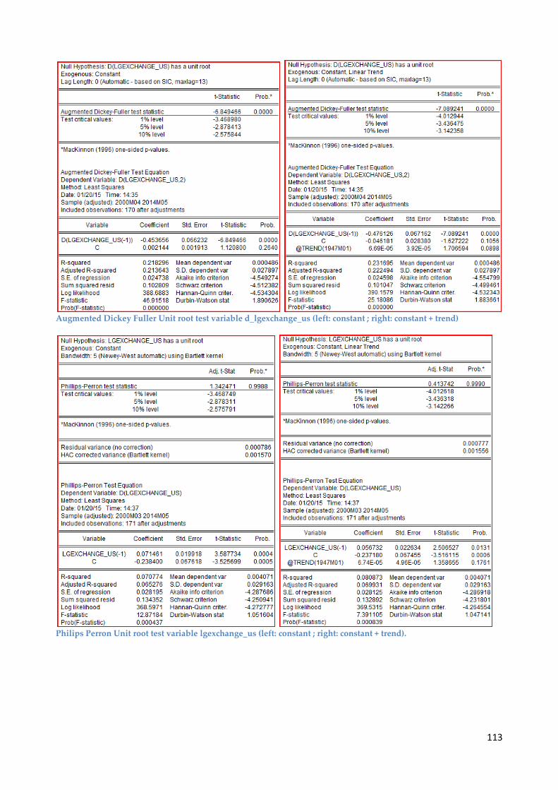
Augmented Dickey Fuller Unit root test variable d_lgexchange_us (left: constant ; right: constant + trend)

Philips Perron Unit root test variable lgexchange_us (left: constant ; right: constant + trend).

113

Philips Perron Unit root test variable d_lgexchange_us (left: constant ; right: constant + trend).

Augmented Dickey Fuller Unit root test variable lgexchange_eu (left: constant ; right: constant + trend)

114

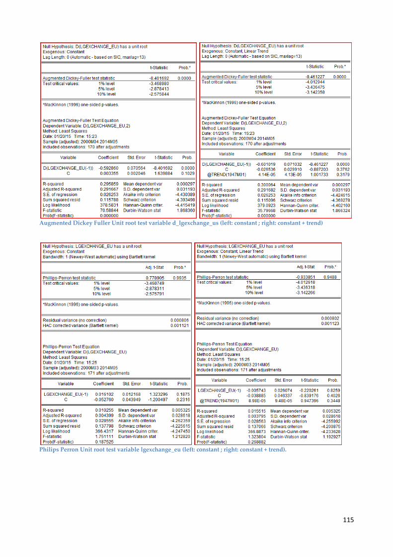
Augmented Dickey Fuller Unit root test variable d_lgexchange_us (left: constant ; right: constant + trend)

Philips Perron Unit root test variable lgexchange_eu (left: constant ; right: constant + trend).

115

Philips Perron Unit root test variable d_lgexchange_eu (left: constant ; right: constant + trend).

Augmented Dickey Fuller Unit root test variable lgtrade_balance_us (left: constant ; right: constant + trend)

116

Augmented Dickey Fuller Unit root test variable d_lgtrade_balance_us (left: constant ; right: constant + trend)

Philips Perron Unit root test variable lgtrade_balance_us (left: constant ; right: constant + trend).

117

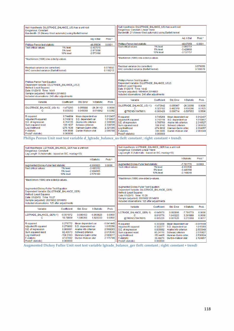
Philips Perron Unit root test variable d_lgtrade_balance_us (left: constant ; right: constant + trend).

Augmented Dickey Fuller Unit root test variable lgtrade_balance_ger (left: constant ; right: constant + trend)

118

Augmented Dickey Fuller Unit root test variable d_lgtrade_balance_ger (left: constant ; right: constant + trend)

Philips Perron Unit root test variable lgtrade_balance_ger (left: constant ; right: constant + trend).

119

Philips Perron Unit root test variable d_lgtrade_balance_ger (left: constant ; right: constant + trend).

Augmented Dickey Fuller Unit root test variable lgoil_price (left: constant ; right: constant + trend)

120

Augmented Dickey Fuller Unit root test variable d_lgoil_price (left: constant ; right: constant + trend)

Philips Perron Unit root test variable lgoil_price (left: constant ; right: constant + trend).

121

Philips Perron Unit root test variable d_lgoil_price (left: constant ; right: constant + trend).

Augmented Dickey Fuller Unit root test variable lggas_price (left: constant ; right: constant + trend)

122

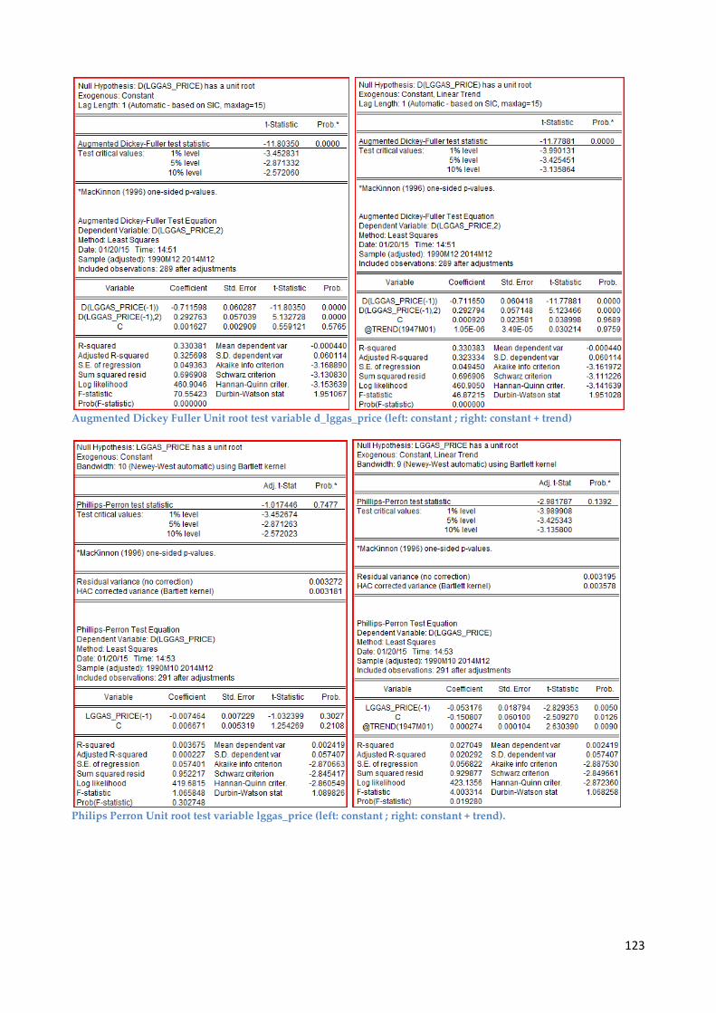
Augmented Dickey Fuller Unit root test variable d_lggas_price (left: constant ; right: constant + trend)

Philips Perron Unit root test variable lggas_price (left: constant ; right: constant + trend).

123

Philips Perron Unit root test variable d_lggas_price (left: constant ; right: constant + trend). Appendix Q: Tables constant D_trade_balance

_us (-1) D_exchange_us (-1)

D_gdp_russia (-1)

D_oil_price (-1)

D_gas_price (-1)

R^2

AR 0.6779 0.0000 0.1509 DL1 0.9016 0.6472 0.0013 DL2 0.9085 0.8785 0.8677 0.0003 DL3 0.9179 0.9149 0.9065 0.0027 0.0701 DL4 0.9131 0.9080 0.8520 0.0680 0.5982 0.0721 ARDL1 0.8697 0.0000 0.5648 0.1542 ARDL2 0.9160 0.0000 0.8171 0.6510 0.1496 ARDL3 0.8166 0.0000 0.8848 0.9212 0.0000 0.2743 ARDL4 0.7879 0.0000 0.8551 0.8807 0.0345 0.0537 0.2960 Table 1. Estimation of the coefficients of Russia’s forecasting models. Also including the 𝑹𝑹𝟐𝟐. constant D_trade_balance

_ger (-1) D_exchange_eu (-1)

D_gdp_russia (-1)

D_oil_price (-1)

D_gas_price (-1)

R^2

AR 0.9667 0.0000 0.2629 DL1 0.9006 0.7054 0.0009 DL2 0.8938 0.3740 0.4958 0.0083 DL3 0.9208 0.4322 0.5389 0.5839 0.0106 DL4 0.9056 0.4570 0.4541 0.2402 0.2558 0.0209 ARDL1 0.9582 0.0000 0.9996 0.2611 ARDL2 0.7846 0.0000 0.5171 0.3590 0.2789 ARDL3 0.8664 0.0000 0.7422 0.4700 0.0758 0.2970 ARDL4 0.8442 0.0000 0.7897 0.3596 0.0171 0.1096 0.3116 Table 2. Estimation of the coefficients of Russia’s forecasting models. Also including the 𝑹𝑹𝟐𝟐.

124

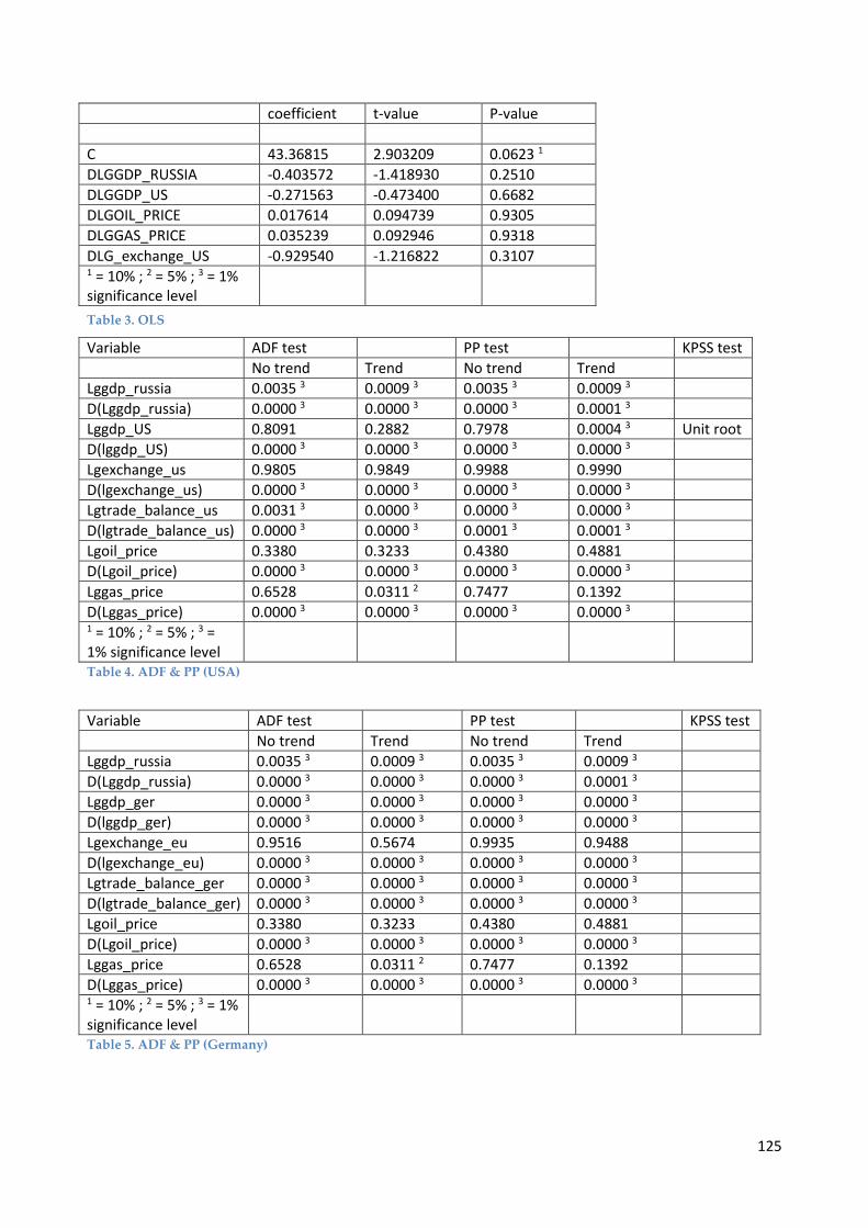
Table 3. OLS

Table 4. ADF & PP (USA)

Table 5. ADF & PP (Germany)

coefficient t-value P-value C 43.36815 2.903209 0.0623 1 DLGGDP_RUSSIA -0.403572 -1.418930 0.2510 DLGGDP_US -0.271563 -0.473400 0.6682 DLGOIL_PRICE 0.017614 0.094739 0.9305 DLGGAS_PRICE 0.035239 0.092946 0.9318 DLG_exchange_US -0.929540 -1.216822 0.3107 1 = 10% ; 2 = 5% ; 3 = 1% significance level

Variable ADF test PP test KPSS test No trend Trend No trend Trend Lggdp_russia 0.0035 3 0.0009 3 0.0035 3 0.0009 3 D(Lggdp_russia) 0.0000 3 0.0000 3 0.0000 3 0.0001 3 Lggdp_US 0.8091 0.2882 0.7978 0.0004 3 Unit root D(lggdp_US) 0.0000 3 0.0000 3 0.0000 3 0.0000 3 Lgexchange_us 0.9805 0.9849 0.9988 0.9990 D(lgexchange_us) 0.0000 3 0.0000 3 0.0000 3 0.0000 3 Lgtrade_balance_us 0.0031 3 0.0000 3 0.0000 3 0.0000 3 D(lgtrade_balance_us) 0.0000 3 0.0000 3 0.0001 3 0.0001 3 Lgoil_price 0.3380 0.3233 0.4380 0.4881 D(Lgoil_price) 0.0000 3 0.0000 3 0.0000 3 0.0000 3 Lggas_price 0.6528 0.0311 2 0.7477 0.1392 D(Lggas_price) 0.0000 3 0.0000 3 0.0000 3 0.0000 3 1 = 10% ; 2 = 5% ; 3 = 1% significance level

Variable ADF test PP test KPSS test No trend Trend No trend Trend Lggdp_russia 0.0035 3 0.0009 3 0.0035 3 0.0009 3 D(Lggdp_russia) 0.0000 3 0.0000 3 0.0000 3 0.0001 3 Lggdp_ger 0.0000 3 0.0000 3 0.0000 3 0.0000 3 D(lggdp_ger) 0.0000 3 0.0000 3 0.0000 3 0.0000 3 Lgexchange_eu 0.9516 0.5674 0.9935 0.9488 D(lgexchange_eu) 0.0000 3 0.0000 3 0.0000 3 0.0000 3 Lgtrade_balance_ger 0.0000 3 0.0000 3 0.0000 3 0.0000 3 D(lgtrade_balance_ger) 0.0000 3 0.0000 3 0.0000 3 0.0000 3 Lgoil_price 0.3380 0.3233 0.4380 0.4881 D(Lgoil_price) 0.0000 3 0.0000 3 0.0000 3 0.0000 3 Lggas_price 0.6528 0.0311 2 0.7477 0.1392 D(Lggas_price) 0.0000 3 0.0000 3 0.0000 3 0.0000 3 1 = 10% ; 2 = 5% ; 3 = 1% significance level

125

Variable t-value p-value RESIDUAL1 -9.565347 0.0000 USE MCKINNON CRITICAL VALUE

-4.43

Table 6. ADF Engle-Granger approach (USA) Variable t-value p-value RESIDUAL1 -1.161536 0.6764 USE MCKINNON CRITICAL VALUE

-4.43

Table 7. ADF Engle-Granger approach (Germany)

Table 8. Johansen cointegration (USA)

Table 9. Johansen cointegration (Germany)

Trace statistic Max-eigen statistic P-value p-value None 0.0092 3 0.1021 At most 1 0.0688 2 0.2702 At most 2 0.1785 0.1224 At most 3 0.6430 0.6839 At most 4 0.6568 0.5742 At most 5 0.8850 0.8850 1 = 10% ; 2 = 5% ; 3 = 1% significance level

Trace statistic Max-eigen statistic P-value p-value None 0.1141 0.0299 2 At most 1 0.7159 0.4545 At most 2 0.9397 0.7440 At most 3 0.9908 0.9773 At most 4 0.9743 0.9897 At most 5 0.3775 0.3775 1 = 10% ; 2 = 5% ; 3 = 1% significance level

126

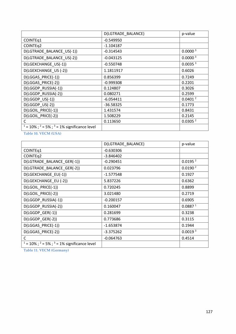
D(LGTRADE_BALANCE) p-value COINTEq1 -0.549950 COINTEq2 -1.104187 D(LGTRADE_BALANCE_US(-1)) -0.314543 0.0000 3 D(LGTRADE_BALANCE_US(-2)) -0.043125 0.0000 3 D(LGEXCHANGE_US(-1)) -0.550748 0.0035 3 D(LGEXCHANGE_US (-2)) 1.1811917 0.6026 D(LGGAS_PRICE(-1)) 0.856399 0.7249 D(LGGAS_PRICE(-2)) -0.999308 0.2201 D(LGGDP_RUSSIA(-1)) 0.124807 0.3026 D(LGGDP_RUSSIA(-2)) 0.080271 0.2599 D(LGGDP_US(-1)) -6.054411 0.0401 2 D(LGGDP_US(-2)) -36.58325 0.1773 D(LGOIL_PRICE(-1)) 1.431574 0.8431 D(LGOIL_PRICE(-2)) 1.508229 0.2145 C 0.113650 0.0305 2 1 = 10% ; 2 = 5% ; 3 = 1% significance level Table 10. VECM (USA) D(LGTRADE_BALANCE) p-value COINTEq1 -0.630306 COINTEq2 -3.846402 D(LGTRADE_BALANCE_GER(-1)) -0.290451 0.0195 2 D(LGTRADE_BALANCE_GER(-2)) 0.023796 0.0190 2 D(LGEXCHANGE_EU(-1)) -1.577548 0.1927 D(LGEXCHANGE_EU (-2)) 5.837226 0.6362 D(LGOIL_PRICE(-1)) 0.720245 0.8899 D(LGOIL_PRICE(-2)) 3.021480 0.2719 D(LGGDP_RUSSIA(-1)) -0.200157 0.6905 D(LGGDP_RUSSIA(-2)) 0.160047 0.0887 1 D(LGGDP_GER(-1)) 0.281699 0.3238 D(LGGDP_GER(-2)) 0.773686 0.3115 D(LGGAS_PRICE(-1)) -1.653874 0.1944 D(LGGAS_PRICE(-2)) -3.375262 0.0019 3 C -0.064763 0.4514 1 = 10% ; 2 = 5% ; 3 = 1% significance level Table 11. VECM (Germany)

127