erasure techniques in mrd codes, by w. b. vasantha kandasamy, florentin smarandache, r. sujatha, r....
TRANSCRIPT

8/2/2019 Erasure Techniques in MRD Codes, by W. B. Vasantha Kandasamy, Florentin Smarandache, R. Sujatha, R. S. Raja …
http://slidepdf.com/reader/full/erasure-techniques-in-mrd-codes-by-w-b-vasantha-kandasamy-florentin-smarandache 1/164

8/2/2019 Erasure Techniques in MRD Codes, by W. B. Vasantha Kandasamy, Florentin Smarandache, R. Sujatha, R. S. Raja …
http://slidepdf.com/reader/full/erasure-techniques-in-mrd-codes-by-w-b-vasantha-kandasamy-florentin-smarandache 2/164
Erasure Techniques
in MRD codes
W. B. Vasantha KandasamyFlorentin Smarandache
R. SujathaR. S. Raja Durai
ZIP PUBLISHINGOhio
2012

8/2/2019 Erasure Techniques in MRD Codes, by W. B. Vasantha Kandasamy, Florentin Smarandache, R. Sujatha, R. S. Raja …
http://slidepdf.com/reader/full/erasure-techniques-in-mrd-codes-by-w-b-vasantha-kandasamy-florentin-smarandache 3/164
2
This book can be ordered from:
Zip Publishing
1313 Chesapeake Ave.Columbus, Ohio 43212, USA
Toll Free: (614) 485-0721E-mail: [email protected] Website: www.zippublishing.com
Copyright 2012 by Zip Publishing and the Authors
Peer reviewers:Professor Paul P. Wang, Ph D, Department of Electrical & Computer Engineering, PrattSchool of Engineering, Duke University, Durham, NC 27708, USAProf. Catalin Barbu, V. Alecsandri National College, Mathematics Department, Bacau,RomaniaFlorentin Popescu, Facultatea de Mecanica, University of Craiova, Romania.
Many books can be downloaded from the followingDigital Library of Science:http://www.gallup.unm.edu/~smarandache/eBooks-otherformats.htm
ISBN-13: 978-1-59973-177-3
EAN: 9781599731773
Printed in the United States of America

8/2/2019 Erasure Techniques in MRD Codes, by W. B. Vasantha Kandasamy, Florentin Smarandache, R. Sujatha, R. S. Raja …
http://slidepdf.com/reader/full/erasure-techniques-in-mrd-codes-by-w-b-vasantha-kandasamy-florentin-smarandache 4/164
3
CONTENTS
Preface 5
Chapter One
BASIC CONCEPTS 7
Chapter Two
ALGEBRAIC LINEAR CODES AND THEIR PROPERTIES 29
Chapter Three
ERASURE DECODING OF MAXIMUM RANK DISTANCE
CODES 49
3.1 Introduction 49
3.2 Maximum Rank Distance Codes 513.3 Erasure Decoding of MRD Codes 54

8/2/2019 Erasure Techniques in MRD Codes, by W. B. Vasantha Kandasamy, Florentin Smarandache, R. Sujatha, R. S. Raja …
http://slidepdf.com/reader/full/erasure-techniques-in-mrd-codes-by-w-b-vasantha-kandasamy-florentin-smarandache 5/164
4
Chapter Four
MRD CODES –SOME PROPERTIES AND A DECODING
TECHNIQUE 63
4.1 Introduction 63
4.2 Error-erasure Decoding Techniques to MRD Codes 64
4.3 Invertible q-Cyclic RD Codes 834.4 Rank Distance Codes With Complementary Duals 101
4.4.1 MRD Codes With Complementary Duals 103
4.4.2 The 2-User F-Adder Channel 1064.4.3 Coding for the 2-user F-Adder Channel 107
Chapter Five
EFFECTIVE ERASURE CODES FOR RELIABLE COMPUTER
COMMUNICATION PROTOCOLS USING CODES OVER
ARBITRARY RINGS 111
5.1 Integer Rank Distance Codes 112
5.2 Maximum Integer Rank Distance Codes 114
Chapter Six
CONCATENATION OF ALGEBRAIC CODES 129
6.1 Concatenation of Linear Block Codes 129
6.2 Concatenation of RD Codes With CR-Metric 140
FURTHER READING 153
INDEX 157
ABOUT THE AUTHORS 161

8/2/2019 Erasure Techniques in MRD Codes, by W. B. Vasantha Kandasamy, Florentin Smarandache, R. Sujatha, R. S. Raja …
http://slidepdf.com/reader/full/erasure-techniques-in-mrd-codes-by-w-b-vasantha-kandasamy-florentin-smarandache 6/164
5
PREFACE
In this book the authors study the erasure techniques in
concatenated Maximum Rank Distance (MRD) codes. The authors for
the first time in this book introduce the new notion of concatenation of
MRD codes with binary codes, where we take the outer code as the RDcode and the binary code as the inner code. The concatenated code
consists of the codewords of the outer code expressed in terms of the
alphabets of the inner code. These new class of codes are defined asCRM codes. This concatenation techniques helps one to construct any
CRM code of desired minimum distance which is not enjoyed by any
other class of codes.Also concatenation of several binary codes are introduced using the
newly defined notion of special blanks. These codes can be used in bulk
transmission of a message into several channels and the completed work is again consolidated and received.
Finally the notion of integer rank distance code is introduced. This
book is organized into six chapters. The first chapter introduces the
basic algebraic structures essential to make this book a self containedone. Algebraic linear codes and their basic properties are discussed in
chapter two. In chapter three the authors study the basic properties of
erasure decoding in maximum rank distance codes.
Some decoding techniques about MRD codes are described anddiscussed in chapter four of this book. Rank distance codes with
complementary duals and MRD codes with complementary duals are

8/2/2019 Erasure Techniques in MRD Codes, by W. B. Vasantha Kandasamy, Florentin Smarandache, R. Sujatha, R. S. Raja …
http://slidepdf.com/reader/full/erasure-techniques-in-mrd-codes-by-w-b-vasantha-kandasamy-florentin-smarandache 7/164
6
introduced and their applications are discussed. Chapter five introduces
the notion of integer rank distance codes. The final chapter introduces
some concatenation techniques.We thank Dr. K.Kandasamy for proof reading and being extremely
supportive.
W.B.VASANTHA KANDASAMY
FLORENTIN SMARANDACHE
R. SUJATHA
R. S. RAJA DURAI

8/2/2019 Erasure Techniques in MRD Codes, by W. B. Vasantha Kandasamy, Florentin Smarandache, R. Sujatha, R. S. Raja …
http://slidepdf.com/reader/full/erasure-techniques-in-mrd-codes-by-w-b-vasantha-kandasamy-florentin-smarandache 8/164
7
Chapter One
BASIC CONCEPTS
In this chapter we give the basic concepts to make this book a
self contained one. Basically we need the notion of vectorspaces over finite fields and the notion of irreducible
polynomials over finite fields. Also the notion of cosets of groups for error correction is needed. We will briefly recall only
those facts, which is essential for a beginner to under standalgebraic coding theory.
DEFINITION 1.1: Let G be a non empty set ‘*’ a closed
associative binary operation defined on G such that;
(i) there exists a unique element e in G with
g * e = e * g = g for all g ∈ G.
(ii) For every g ∈ G there exists a unique g′ in G
such that g * g′ = g′ * g = e;
g′ is called the inverse of g in G under the
binary operation *.
Then (G, *) is defined as a group.

8/2/2019 Erasure Techniques in MRD Codes, by W. B. Vasantha Kandasamy, Florentin Smarandache, R. Sujatha, R. S. Raja …
http://slidepdf.com/reader/full/erasure-techniques-in-mrd-codes-by-w-b-vasantha-kandasamy-florentin-smarandache 9/164
8
If in G for every pair a, b ∈ G; a*b = b*a then we say G is
an abelian group.
If the number of distinct elements in G is finite then G issaid to be a finite group otherwise G is said to be an infinite
group.
Example 1.1: Z2 = {0, 1} is an additive abelian group given by
the following table:
0 1
0 0 11 1 0
+
Z2 under multiplication is not a group.
Example 1.2: (Z3, +) is an abelian group of order 3 given by the
following table:
0 1 2
0 0 1 2
1 1 2 0
2 2 0 1
+
Example 1.3: (Zn, +), (1 < n < ∞) is an abelian group of order n.
Example 1.4: G = Z2 × Z2 × Z2 = {(a, b, c) / a, b, c ∈ Z2} is agroup under addition modulo 2. G is of order 8.
Example 1.5: Let G = Z2 × Z2 × … × Z2, n times with
G = {(x1, x2, …, xn) / xi ∈ Z2; 1 ≤ i ≤ n}is an abelian group under addition modulo 2 of order 2
n.
Example 1.6: H = Zp × Zp × … × Zp - t times is an abelian group
under addition modulo p of order p
t
.
Now we will just define the notion of a subgroup.

8/2/2019 Erasure Techniques in MRD Codes, by W. B. Vasantha Kandasamy, Florentin Smarandache, R. Sujatha, R. S. Raja …
http://slidepdf.com/reader/full/erasure-techniques-in-mrd-codes-by-w-b-vasantha-kandasamy-florentin-smarandache 10/164
9
DEFINITION 1.2: Let (G, *) be a group. H a proper subset of G.
If (H, *) is a group then, we call H to be a subgroup of G.
Example 1.7: Let G = (Z12, +) be a group. H = {0, 2, 4, 6, 8, 10}
⊆ Z12 under + is a subgroup of G.
Example 1.8: Let (Z, +) be a group under addition (Z the set of
positive, negative integers with zero) (3Z, +) ⊆ (Z, +) is asubgroup of G.
Example 1.9: Let (Q, +) be a group under addition. Q the set of rationals. Q is an abelian group of infinite order.
(Z, +) ⊆ (Q, +) is a subgroup, (Z, +) is also of infinite order.(Q, +) has no subgroup of finite order.
Example 1.10: Let (R, +) be the group under addition. (R, +) is
an infinite abelian group. (R, +) has infinitely many subgroups
of infinite order.
Example 1.11: Let (R \ {0}, ×) be a group under multiplicationof infinite order. Clearly R \ {0} is an abelian group;
H = {1, –1} ⊆ R \ {0} is a subgroup of R \ {0} of order two.
Example 1.12: G = (Q \ {0}, ×) is an abelian group of infinite
order. H = {1, –1} ⊆ (Q \ {0}, ×) is a subgroup of finite order inG.
Interested reader can refer and read the classical results ongroups [2].
Now we proceed onto define normal subgroup of a group.
DEFINITION 1.3: Let (G, *) be a group. (H, *) be a subgroup of
G we say, H is a normal subgroup of G if gH = Hg or gHg-1
=
H for all g ∈ G.

8/2/2019 Erasure Techniques in MRD Codes, by W. B. Vasantha Kandasamy, Florentin Smarandache, R. Sujatha, R. S. Raja …
http://slidepdf.com/reader/full/erasure-techniques-in-mrd-codes-by-w-b-vasantha-kandasamy-florentin-smarandache 11/164
10
We will illustrate this with examples. First it is important to
note that in case of commutative groups every subgroup isnormal.
We have so far given only examples of groups which are
commutative.
Example 1.13: Let
G =a b
c d
ad – bc ≠ 0, a, b, c, d ∈ Q
+ ∪ {0}}.
G is a non commutative group under multiplication of
matrices.
It is easily verified all subgroups of G are not normal in G,
However H =x 0
0 x
x ∈ Q+} is a subgroup of G and H
is not a normal in G.
Also P =x 0
x, y Q0 y
+
∈
is a subgroup of G and is P
not a normal subgroup of G.
We now proceed onto recall the definition of cosets of a
group.
DEFINITION 1.4: Let G be a group H a subgroup of G. For
a ∈ G, aH = {ah | h ∈ H} is defined as the right coset of H in G.
We have the following properties to be true.
(i) There is a one to one correspondence between any
two right cosets of H in G.

8/2/2019 Erasure Techniques in MRD Codes, by W. B. Vasantha Kandasamy, Florentin Smarandache, R. Sujatha, R. S. Raja …
http://slidepdf.com/reader/full/erasure-techniques-in-mrd-codes-by-w-b-vasantha-kandasamy-florentin-smarandache 12/164
11
(ii) In case H is a normal subgroup of G we have the
right coset to be equal with the left coset.
If H is a normal subgroup of G we can define the quotientgroup or the factor group of H in G as
G/H = {Hb / b ∈ G}
= {bH / b ∈ G} (Hb = bH for all b ∈ G}.
G/H is a group and if G is finite o (G) / o (H) = o (G/H).
Now we proceed onto recall definition of rings and fields.
DEFINITION 1.5: Let R be a non empty set with the two binary
operations + and × , such that
(i) (R, +) is an abelian group
(ii) (R, × ) is such that ‘× ’ is a closed operation on
R and ‘× ’ is an associative binary operation on
R
(iii) If for all a, b, c ∈ R we have
a × (b+c) = a × b + a × c and (b+c) × a
= b × a + c × a;
then (R, +, × ) is defined to be a ring.
If a × b = b × a for all a, b ∈ R, we define R to be a
commutative ring.
If R contains 1 called the multiplicative identity such that
a × 1 = 1 × a = a for all a ∈ R we define R to be a ring with
unit.
If is important to note that all rings need not be rings with
unit.
We will give examples of them.

8/2/2019 Erasure Techniques in MRD Codes, by W. B. Vasantha Kandasamy, Florentin Smarandache, R. Sujatha, R. S. Raja …
http://slidepdf.com/reader/full/erasure-techniques-in-mrd-codes-by-w-b-vasantha-kandasamy-florentin-smarandache 13/164
12
Example 1.14: Let R = (Z, +, ×); R is a commutative ring withunit.
Example 1.15: Consider Z15; Z15 under modulo addition andmodulo multiplication is a commutative ring with unit.
Example 1.16: Consider Z2 = {0, 1}; Z2 is a commutative ringwith unit.
Example 1.17: Let Z3 = {0, 1, 2} be the commutative ring withunit.
Example 1.18: Let 3Z = {3n / n ∈ Z}, 3Z be a commutativering but 3Z does not contain the unit 1.
Example 1.19: Let 5Z be the commutative ring, but 5Z is a ring
and does not contain the unit.
Example 1.20: (Q, +, ×) is a commutative ring with unit.
Example 1.21: R =a b
a,b,c,d Z, ,c d
∈ + ×
is a non
commutative ring with identity1 0
0 1
under matrix
multiplication ×.
Example 1.22: Let P = {n × n matrices with entries from Q},P is a non commutative ring with unit under matrix addition and
multiplication.
We will now recall the definitions of subrings and ideals of a ring.
DEFINITION 1.6: Let (R, +, × ) be a ring. Suppose φ ≠ S ⊆ R be
a proper subset of R. If (S, +, × ) is a ring, we define S to be a
subring of R.

8/2/2019 Erasure Techniques in MRD Codes, by W. B. Vasantha Kandasamy, Florentin Smarandache, R. Sujatha, R. S. Raja …
http://slidepdf.com/reader/full/erasure-techniques-in-mrd-codes-by-w-b-vasantha-kandasamy-florentin-smarandache 14/164
13
We will illustrate this situation by some examples.
Example 1.23: Let R = (Z, +, ×) be a ring; S = (3Z, +, ×) is a
subring of R.
Example 1.24: Let S = (Z, +, ×) be the ring of integers,
P = {12Z, +, ×} is a subring of S.
It is important and interesting to note that a subring of S
need not in general have the unit however the ring S has unit.
This is a marked difference between a subgroup of a group,for a subgroup must contain the identity but a subring need notcontain the unit 1 with respect to multiplication. Examples 1.23
and 1.24 give subrings of (Z, +, ×) which do not contain 1, theunit of Z.
Example 1.25: Let R = (Q, +, ×) be a ring. (Z, +, ×) is a subring
and it contains the unit. However (8Z, +, ×) is also a subring of
(Q, +, ×) but (8Z, +, ×) does not contain the unit 1 of R.
We have seen subrings of a ring. All rings given are of
infinite order except those given in examples 1.15, 1.16 and1.17.
Example 1.26: Let Z30 be the ring. S = {0, 10, 20} ⊆ Z30 is a
subring and 1 ∉ S.
Example 1.27: Let Z12 be the ring. ConsiderP = {0, 2, 4, 6, 8, 10}, P is a subring of Z12. P does not contain
the unit 1.
Example 1.28: Let Z5 be the ring. Z5 has no proper subrings.Only 0 and Z5 are the subrings of Z5.
Example 1.29: Let Z8 = {0, 1, 2, 3, …, 7} be a ring. Consider
H = {0, 4} ⊆ Z8, H is a subring of Z
8and H does not contain the
unit.

8/2/2019 Erasure Techniques in MRD Codes, by W. B. Vasantha Kandasamy, Florentin Smarandache, R. Sujatha, R. S. Raja …
http://slidepdf.com/reader/full/erasure-techniques-in-mrd-codes-by-w-b-vasantha-kandasamy-florentin-smarandache 15/164
14
Example 1.30: Zn = {0, 1, 2, …, n–1} (n < ∞) is thecommutative ring with unit having n elements. If n is a prime,
Zn has no proper subrings.
DEFINITION 1.7: Let R be a ring. H be a subring of R. If for all
r ∈ R and h ∈ H; rh ∈ H then we define H to be left ideal.
Similarly if for all r ∈ R and h ∈ H, hr ∈ H we define H to
be a right ideal. If H is both a left ideal and a right ideal then
we define H to be an ideal of R.
The following observations are important.
(i) If R is a commutative ring the notion of right
ideal and left ideal coincides.
(ii) If I is an ideal of a ring R then (0) ∈ I.
(iii) (0) is called the zero ideal of R.
(iv) If I is an ideal of the ring R then 1 the unit of Ris not in I.
For if 1 ∈ I then I = R.
We will now give examples of ideals.
Example 1.31: Let (Z, +, ×) be the ring of integers. 2Z is anideal of Z.
Example 1.32: Let (Q, +, ×) be the ring the rationals, Q has noproper ideals.
Example 1.33: Let (R, +, ×) be the ring of reals. R has noproper ideals.
Example 1.34: Let (Z, +, ×) be the ring of integers, nZ is an
ideal of Z for n = 2, 3, …, ∞.
8/2/2019 Erasure Techniques in MRD Codes, by W. B. Vasantha Kandasamy, Florentin Smarandache, R. Sujatha, R. S. Raja …
http://slidepdf.com/reader/full/erasure-techniques-in-mrd-codes-by-w-b-vasantha-kandasamy-florentin-smarandache 16/164
15
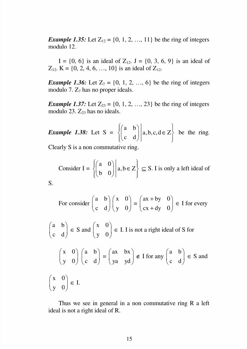
Example 1.35: Let Z12 = {0, 1, 2, …, 11} be the ring of integers
modulo 12.
I = {0, 6} is an ideal of Z12. J = {0, 3, 6, 9} is an ideal of Z12. K = {0, 2, 4, 6, …, 10} is an ideal of Z12.
Example 1.36: Let Z7 = {0, 1, 2, …, 6} be the ring of integers
modulo 7. Z7 has no proper ideals.
Example 1.37: Let Z23 = {0, 1, 2, …, 23} be the ring of integers
modulo 23. Z23 has no ideals.
Example 1.38: Let S =a b
a,b,c,d Zc d
∈
be the ring.
Clearly S is a non commutative ring.
Consider I =a 0
a,b Zb 0
∈
⊆ S. I is only a left ideal of
S.
For considera b
c d
x 0
y 0
=ax by 0
cx dy 0
+
+ ∈ I for every
a b
c d
∈ S andx 0
y 0
∈ I. I is not a right ideal of S for
x 0
y 0
a b
c d
=ax bx
ya yd
∉ I for anya b
c d
∈ S and
x 0
y 0
∈ I.
Thus we see in general in a non commutative ring R a leftideal is not a right ideal of R.

8/2/2019 Erasure Techniques in MRD Codes, by W. B. Vasantha Kandasamy, Florentin Smarandache, R. Sujatha, R. S. Raja …
http://slidepdf.com/reader/full/erasure-techniques-in-mrd-codes-by-w-b-vasantha-kandasamy-florentin-smarandache 17/164
16
Now just like quotient groups we can define quotient rings
using two sided ideals of the ring R. Let R be a ring and I a two
sided ideal of R. R/I = {a + I / a ∈ R} is a ring defined as the
quotient ring of R [2].
We will illustrate this situation by some examples.
Example 1.39: Let Z be the ring. I = 2Z is an ideal of Z. Z/2Z=I
= {I, 1 + I}. Clearly I acts as the additive identity for Z/I. Since
1 + I + I = 1 + (I+I) = 1 + I, as I is an ideal, I + I = I. Further(1+I) is the unit in Z/I for (1+I) (1+I) = 1+I + 1.I = 1+I.
Thus Z/I is a ring and Z/2Z = Z/I is isomorphic with Z 2. For
0 I and 1 1+I so Z2 ≅ Z/I = {I, 1+I}.
Example 1.40: Let Z be the ring. I = 5Z be the ideal of Z.
Z/I = Z/5Z = {I, 1+I, 2+I, 3+I, 4+I} is the quotient ring.
Example 1.41: Let Z be the ring. nZ = I be the ideal of Z.Z/I = {I, 1+I, 2+I, …, n–1 + I} is the quotient ring.
Example 1.42: Let Z12 be the ring of modulo integers.
I = {0, 6} be an ideal of Z12.
Z12 /I = {I, 1+I, 2+I, 3+I, 4+I, 5+I} is the quotient ring.
Now we have seen examples of quotient rings.
We proceed onto recall the definition of a field.
DEFINITION 1.8: Let (F, +, × ) be such that F is a non empty set.
If
(i) (F, +) is an abelian group under addition,
(ii) {F \ {0}, × } is an abelian group under multiplication
and

8/2/2019 Erasure Techniques in MRD Codes, by W. B. Vasantha Kandasamy, Florentin Smarandache, R. Sujatha, R. S. Raja …
http://slidepdf.com/reader/full/erasure-techniques-in-mrd-codes-by-w-b-vasantha-kandasamy-florentin-smarandache 18/164
17
(iii) if a × (b+c) = ab + ac for all a, b, c ∈ F, then we define
F to be a field.
If in F we have nx = 0 for all x ∈ F only if n = 0 where n isany positive integer then we say F is a field of characteristic
zero.
If for some n; nx = 0 for all x ∈ F where n is the smallest
such number then we say F is a field of characteristic n. Clearly
n will only be a prime.
We will now proceed onto give examples of fields.
Example 1.43: Let Z5 = {0, 1, 2, 3, 4} be a field and Z5 is a field
of characteristic 5.
Example 1.44: Let Z43 = {0, 1, 2, …, 42} be a field and is of characteristic 43.
Example 1.45: (Q, +, ×) is a field and is a field of characteristic
zero.
Example 1.46: (R, +, ×) is a field and is of characteristic zeroand we see the set of integers, Z is not a field, only a ring.
Example 1.47: Z15 is not a field only a ring as 3.5 ≡ 0 (mod 15)so Z15 \ {0} is not a group.
It is easily verified that every field is a ring and a ring ingeneral is not a field.
We recall the definition of a subfield.
DEFINITION 1.9: Let (F, +, × ) be a field. A proper subset P ⊆ F
such that if (P, +, × ) is a field, then we define P to be a subfield,
of F. If F has no subfield then we call F to be a prime field.
We will give examples of prime fields.
8/2/2019 Erasure Techniques in MRD Codes, by W. B. Vasantha Kandasamy, Florentin Smarandache, R. Sujatha, R. S. Raja …
http://slidepdf.com/reader/full/erasure-techniques-in-mrd-codes-by-w-b-vasantha-kandasamy-florentin-smarandache 19/164
18
Example 1.48: Let Q be the field. Q has no proper subfield.
Hence Q is the prime field of characteristic zero.
Example 1.49: Let (R, +, ×) be the field of reals, R is not aprime field of characteristic zero as (Q, +, ×) ⊆ (R, +, ×) is aproper subfield of R.
Example 1.50: Z2 = {0, 1} is the prime field of characteristic
two as Z2 has no proper subfields.
Example 1.51: Z3 = {0, 1, 2} is the prime field of characteristic
three. Z3 has no proper subfields.
Example 1.52: Z17 = {0, 1, 2, …, 16} is the prime field of
characteristic 17.
Example 1.53: Zp = {0, 1, 2, …, p–1} is the prime field of
characteristic p, p a prime.
Now it is an interesting fact that fields cannot have ideals in
them. This work is left as an exercise to the reader [2].
Now we see we do not have non prime fields of finite
characteristic p, p a prime; we proceed on to give methods for
constructing them.
We will recall the definition of polynomial rings.
DEFINITION 1.10:
Let R be a commutative ring with unit. x an
indeterminate;
R[x] =∞
=
∈
∑ i
i i
i 0
a x a R ,
R[x] under usual polynomial addition and multiplication is a
ring called the polynomial ring. R[x] is a again a commutative
ring with unit and R ⊆ R[x].

8/2/2019 Erasure Techniques in MRD Codes, by W. B. Vasantha Kandasamy, Florentin Smarandache, R. Sujatha, R. S. Raja …
http://slidepdf.com/reader/full/erasure-techniques-in-mrd-codes-by-w-b-vasantha-kandasamy-florentin-smarandache 20/164
19
We will give examples of them.
Example 1.54: Let R be the field of reals. R[x] is the
polynomial ring in the indeterminate x.
Clearly R[x] is not a field; R[x] is only a commutative ringwith unit.
Example 1.55: Let Q be the field of rationals. Q[x] is thepolynomial ring.
Example 1.56: Let Z2 be the field of characteristic two.
Z2[x] is the polynomial ring.
Example 1.57: Let Z be the ring of integers. Z[x] is thepolynomial ring.
Example 1.58: Let Z5 be the field of characteristic five. Z5[x] isthe polynomial ring.
Example 1.59: Let Z6 be the ring of integers modulo 6. Z6[x] isthe polynomial ring.
Example 1.60: Z2 [x] is the polynomial ring; let p(x) = x2
+ 1 be
in Z2[x]; p(x) is reducible in Z2 [x] for p(x) = (x+1)2.
Consider q(x) = x2
+ x + 1 ∈ Z2[x]; q(x) is irreducible asq(x) cannot be written as the product of polynomials of degree
one in Z2[x].
Inview of this we will define the notion of reducible
polynomial and irreducible polynomial.
Let p(x) ∈ R[x] be a polynomial of degree n in R[x] with
coefficients from R. We say p(x) is reducible in R[x] if p(x) =g(x) b(x) where g(x) and b(x) are polynomials in R(x) with deg
g(x) < deg p(x) and deg b(x) < deg p(x).

8/2/2019 Erasure Techniques in MRD Codes, by W. B. Vasantha Kandasamy, Florentin Smarandache, R. Sujatha, R. S. Raja …
http://slidepdf.com/reader/full/erasure-techniques-in-mrd-codes-by-w-b-vasantha-kandasamy-florentin-smarandache 21/164
20
If p(x) is not reducible that is p(x) = g(x) b(x) implies
deg g(x) = deg p(x) or deg b(x) = deg p(x) then we define p(x)to be irreducible in R[x].
p(x) = x2
+ 1 ∈ R[x]; R reals is an irreducible polynomial inR[x].
p (x) = x2
+ 1 ∈ Z2 [x] is reducible in Z2 [x] as
p(x) = (x+1) (x+1).
p(x) = x
2
– 4 ∈ R[x] is a reducible polynomial asx2
– 4 = (x+2) (x–2) where R is the set of reals.
p (x) = x2
+ q is irreducible polynomial in R[x] where q is a
positive value in R, R-reals.
We have seen examples of reducible and irreducible
polynomials.
We first see the concept of reducibility or irreducibility isdependent on the ring or the field over which they are defined.
The purpose of these irreducible polynomials is they generate a
maximal ideal and this concept will be used in the constructionof fields and finite fields.
Let Z[x] be the polynomial ring. x2
+ 1 is a irreduciblepolynomial in Z[x].
Let I be the ideal generated by x2
+ 1. ThusI = {all polynomials of degree greater than or equal to two}
Z[x]
I= {I, b+I, ax + I, (b + ax) + I / a, b ∈ Z}
= {a + bx + I / a, b ∈ Z}.
Suppose we replace Z by Z2 and consider the polynomialring Z2 [x]; x2 + 1 is a reducible polynomial in Z2 [x].

8/2/2019 Erasure Techniques in MRD Codes, by W. B. Vasantha Kandasamy, Florentin Smarandache, R. Sujatha, R. S. Raja …
http://slidepdf.com/reader/full/erasure-techniques-in-mrd-codes-by-w-b-vasantha-kandasamy-florentin-smarandache 22/164
21
Let I be the ideal generated by x2
+ 1.
Consider
2Z [x]
I = {I, 1 + I, x + I, x + 1 + I}
I acts as the additive identity 1 + I acts as the multiplicative
identity.
Clearly 2Z [x]
Iis not a field; for
(1 + x + I) (1 + x + I) = (1 + x)2 + I = x2 + 1 + I = I is a zero
divisor so 2Z [x]
Iis only a ring.
Now if we consider p(x) = x2
+ x + 1 ∈ Z2[x], clearly p(x) isirreducible in Z2[x].
We see 2 2
2Z [x] Z [x]
x x 1 I=
⟨ + + ⟩
= {I, 1 + I, x + I, 1 + x + I}
where I is the ideal generated by p(x) and I acts as the additive
identity.
Now 1 + I is the multiplicative identity.
Further x + I is the inverse of 1 + x + I. To prove this we
must show
(x + I) (1 + x + I) = 1 + I.
Now (x + I) (1 + x + I) =
x (1 + x) + I = x2
+ x + I
= (x2 + x + 1) + 1 + I
= 1 + I as 1 + x + x2 ∈ I.

8/2/2019 Erasure Techniques in MRD Codes, by W. B. Vasantha Kandasamy, Florentin Smarandache, R. Sujatha, R. S. Raja …
http://slidepdf.com/reader/full/erasure-techniques-in-mrd-codes-by-w-b-vasantha-kandasamy-florentin-smarandache 23/164
22
Thus 2Z [x]
Iis a field with four elements and is of
characteristic two so 2Z [x]
Iis not a prime field of characteristic
two as P = {I, 1+I} ⊆ 2Z [x]
Iis a subfield of 2Z [x]
I.
Now based on this we give the following facts interested
reader can refer [2].
Let Zp[x] be a polynomial ring with coefficients from the
field Zp, p a prime. p (x) ∈ Zp[x] be a polynomial of degree n.Suppose p(x) is irreducible over Zp and I be the ideal generated
by p (x).
NowpZ [x]
Iis a field and this field has p
nelements in it and
its characteristic is p.
Thus this method gives one the way of constructing non
prime fields of characteristic p.
Suppose V = 2
3
Z [x]
I x x 1= ⟨ + + ⟩
= {I, 1 + I, x + I, x2+ I, 1 + x + I, 1 + x
2+ I, x + x
2+ I,
1 + x + x2 + I}.
V = 2Z [x]
Iis a field of characteristic two and V has 2
3
elements and the irreducible polynomial x3
+ x + 1 is of degree
3 so V has 23
elements in it. Suppose p(x) = x3
+ 1, clearly p(x)
is reducible in Z2[x] for x3
+ 1 = (x + 1) (x2+ x + 1).

8/2/2019 Erasure Techniques in MRD Codes, by W. B. Vasantha Kandasamy, Florentin Smarandache, R. Sujatha, R. S. Raja …
http://slidepdf.com/reader/full/erasure-techniques-in-mrd-codes-by-w-b-vasantha-kandasamy-florentin-smarandache 24/164
23
Consider 2 2Z [x] Z [x]
p(x) I=
⟨ ⟩= V = {I, 1 + I, x + I, x
2+ I,
1 + x + I, 1 + x2
+ I, x + x2
+ I, 1 + x + x2
+ I}. V is not a field
for V has zero divisors. I is the additive identity or zero in V.
Consider 1 + x + I, 1 + x + x2
+ I in V. (1+x+I) (1+ x2+x) = I
(using the fact I is an ideal of Z2 [x] so (x+1) I = I and (1+x+x2)I
= I and I + I + I).
(1 + x) (1 + x2+ x) + I = 1 + x
2+ x + x + x
2+ x
3+ I = 1 + x
3+ I
(as 2x = 0 and 2x2
= 0)
= I as 1 + x3 ∈ I.
Thus V has zero divisors; so V is not a field only a ring as
p(x) is a reducible polynomial.
Thus we wish to make a mention that the ideals generated
by a single element will be known as principal ideals. Also we
expect the reader to be familiar with the notion of minimal
ideals, maximal ideals and prime ideals.
However we just give some examples of them.
Example 1.61: Let Z12 = {0, 1, 2, …, 11} be the ring of modulo
integers.
Consider I = {0, 2, 4, 6, 8, 10} ⊆ Z12 to be a maximal ideal
of Z12. Take J = {0, 6} ⊆ Z12, J is a minimal ideal of Z12.
However K = {0, 3, 6, 9} ⊆ Z12 is also a maximal ideal. T = {0,4, 8} ⊆ Z12 is also a minimal ideal of Z12. Thus a ring can havemany maximal ideals and many minimal ideals.
However we show a ring which has no minimal ideals.
Example 1.62: Let Z be the ring of integers. Z has several
maximal ideals, pZ is a maximal ideal where p is a prime.

8/2/2019 Erasure Techniques in MRD Codes, by W. B. Vasantha Kandasamy, Florentin Smarandache, R. Sujatha, R. S. Raja …
http://slidepdf.com/reader/full/erasure-techniques-in-mrd-codes-by-w-b-vasantha-kandasamy-florentin-smarandache 25/164
24
For all primes p we obtain an infinite collection of maximal
ideals.
However Z has no minimal ideal but it has infinite numberof ideals which are neither maximal nor minimal. For nZ when
n is a non prime is neither a maximal nor a minimal ideal.
2Z, 5Z, 3Z, 7Z, 11Z are maximal ideals.
When R is a commutative ring with unit and I a maximal
ideal of R; then R / I is a field.
This property is used in the construction of finite fields of
desired order.
We consider Zp[x]; p a prime Zp[x], the polynomial ring.I be the ideal generated by an irreducible polynomial p(x); then
pZ [x]
I
is a field.
If p(x) is of degree n then Zp [x] / I is a field of ordern
pZ .
Thus this method helps us in generating finite fields which
are not prime.
We will give some examples.
Example 1.63: Let Z5 [x] be the polynomial ring.
Consider p(x) = x2
+ x + 1 in Z5[x]. p(x) is irreducible in
Z5[x]. Let I be the ideal generated by p(x). Now
Z5[x] / I = {I, 1 + I, 2 + I, 3 + I, 4 + I, x + I, 2x + I, 3x + I,
4x + I, 1 + x + I, 2x + 3 + I, …, 4x + 4 + I}. It is easily verified
Z5[x] / I is a field with 25 elements in it.
8/2/2019 Erasure Techniques in MRD Codes, by W. B. Vasantha Kandasamy, Florentin Smarandache, R. Sujatha, R. S. Raja …
http://slidepdf.com/reader/full/erasure-techniques-in-mrd-codes-by-w-b-vasantha-kandasamy-florentin-smarandache 26/164
25
However Z5 [x] / I is not a prime field for it has a subfield
{I, 1 + I, 2 + I, 3 + I, 4 + I} ≅ Z5.
But characteristic of the field Z5 [x] / I is five.
Now if we take p(x) = x2
+ 2x + 2, we see p(x) is a
reducible polynomial in Z5[x]. For (x + 3) (x + 4) = x2
+ 2x + 2.So –3, –4 or 1, 2 are the roots of p(x).
Z5[x] / I = ⟨p(x)⟩ = {I, 1 + I, 2 + I, …, x + 3 + I, x + 4 + I} isnot a field only a commutative ring with unit 1 + I.
For consider x + 3 + I and x + 4 + I in Z5[x] / I.
(x + 3 + I) (x + 4 + I) = (x + 3) (x + 4) + I= x
2+ 2x + 2 + I
= I.
(I is the zero element in Z5[x] / I).
Hence Z5 [x] / I cannot be a field.
Likewise we can create fields or rings of finite order.
Notation: If p(x) = a0 + a1x + … + anxn then p(x) has a
representation in n + 1 tuples given by (a0, a1, …, an), ai’s arecoefficients using which the polynomial ring R[x] is defined
and p(x) ∈ R[x].
Now we just recall the definition of a primitive polynomial.
A polynomial p(x) = a0 + a1x + … + anxn in R[x] is said to
be a primitive polynomial (where a0, a1, …, an are integers) if
the greatest common divisor of a0, a1, …, an is 1.
We will use this concept also in the construction of linear
codes. Now we proceed onto recall the definition of vector
space as we associate or define the algebraic code as a subspace
of a vector space.

8/2/2019 Erasure Techniques in MRD Codes, by W. B. Vasantha Kandasamy, Florentin Smarandache, R. Sujatha, R. S. Raja …
http://slidepdf.com/reader/full/erasure-techniques-in-mrd-codes-by-w-b-vasantha-kandasamy-florentin-smarandache 27/164
26
DEFINITION 1.11: Let V be an additive abelian group. F a field.
We say V is a vector space over the field F if the following
conditions are true.
(1) For every v ∈ V and a ∈ F we have av and va are
in V (av = va and conventionally we write as av a is
called the scalar and v a vector).
(2) a (v1 + v2 ) = av1 + av2 .
(3) (a+b) v = av + bv.
(4) a (bv) = (ab) v.
(5) 1.v = v for all a, b ∈ F and v1 , v2 , v ∈ V and
0.v = 0 ∈ V.
(Here 1 represents the unit element of F).
We give examples of vector spaces.
Example 1.64: Let V = Z2 × Z2 × Z2 × Z2 be a group underaddition, V is a vector space over the field Z2.
Example 1.65: Let V = Q[x] be an additive abelian group. V is
a vector space over the field Q.
Example 1.66: Let V = Z2[x], polynomial group under addition.
V is a vector space over Z2.
We recall the definition of a vector subspace of a vector
space.
DEFINITION 1.12: Let V be a vector space over the field F.
W ⊆ V be a proper subset of V. If W itself is a vector space over
the field F then we call W to be vector subspace of V over the
field F.
We will illustrate this situation by some examples.

8/2/2019 Erasure Techniques in MRD Codes, by W. B. Vasantha Kandasamy, Florentin Smarandache, R. Sujatha, R. S. Raja …
http://slidepdf.com/reader/full/erasure-techniques-in-mrd-codes-by-w-b-vasantha-kandasamy-florentin-smarandache 28/164
27
Example 1.67: Let V = Z2 × Z2 × Z2 × Z2 be a vector space over
the field Z2. Consider W = {Z2 × {0} × Z2 × {0}} ⊆ V; W is avector subspace of V over Z2.
Example 1.68: Let V = Q[x] be the vector space over Q.
Consider
P = 2i
i i
i 0
a x a Q∞
=
∈
∑ ⊆ V;
P is a vector subspace of V over Q.
Example 1.69: Let V = Q × Q × Q × Q × Q × Q be a vector
space over Q. Consider W = Q × {0} × Q × {0} × Q × Q ⊆ V;W is a vector subspace of V over Q.
Example 1.70: Let V = R × R × R × R × R be a vector spaceover Q. Consider
W = Q × Q × Q × Q × Q ⊆ R × R × R × R × R; W is avector subspace of V over Q.
Now the reader is expected to recall the definition of basisand dimension of a vector space [2, 16].
We will be using only finite dimensional vector spaces that
too defined over the finite field. Infact we will be mainly using
the field Z2 orn
2Z of order 2n
and of characteristic two; denotedby GF(2
n) as most of the messages transmitted are binary, it is
sufficient to study over Z2 or GF(2n).
Now we just recall the definition of Hamming distance and
Hamming weight in vector spaces.
We say for any two vectors v1 = (x1, …, xn) and v2 = (y1,
…,yn); v
1and v
2 ∈ V = F × … × F; n-times where F is a field
and V is a vector space over F. The Hamming distance between

8/2/2019 Erasure Techniques in MRD Codes, by W. B. Vasantha Kandasamy, Florentin Smarandache, R. Sujatha, R. S. Raja …
http://slidepdf.com/reader/full/erasure-techniques-in-mrd-codes-by-w-b-vasantha-kandasamy-florentin-smarandache 29/164
28
v1 and v2 denoted by d (v1, v2) = number of places in which
v1 is different from v2.
For instance if v1 = (1 0 0 1 0 0 1) and v2 = (0 1 1 1 0 0 1)then the Hamming distance between v1 and v2 denoted by
d (v1, v2) = 3.
Now Hamming weight x of a vector in V is the distance of x
from the zero vector. Thus Hamming weight of x is the numberof non zero co ordinates in the vector x, thus d(x, 0) = w(x) =
number of non zero coordinates in x.
Thus if x = (1 0 1 0 1 0 0 1 1 1) be a vector in V then
w(x) = d (x, 0) = 6.
Now having defined Hamming weight and Hammingdistance we now proceed onto define linear codes and illustrate
them with examples in chapter two.

8/2/2019 Erasure Techniques in MRD Codes, by W. B. Vasantha Kandasamy, Florentin Smarandache, R. Sujatha, R. S. Raja …
http://slidepdf.com/reader/full/erasure-techniques-in-mrd-codes-by-w-b-vasantha-kandasamy-florentin-smarandache 30/164
29
Chapter Two
ALGEBRAIC LINEAR CODES AND
THEIR PROPERTIES
In this chapter we recall the definition of algebraic linear
codes and discuss the various properties associated with them.
We give examples and define several types of codes.
Let x = (x1, x2, …, xn) where xi ∈Fq, where Fq is a finitefield. (q, a power of a prime). In x the first k symbols are taken
as message symbols and the remaining n – k elements xk+1, xk+2,…, xn are check symbols (or control symbols). x = (x1, …, xn)is defined as the code word and it can be denoted by (x1, …, xn)
or x1 x2 … xn or x1, x2 , …, xn.
We will now roughly indicate how messages go through the
system starting from the sender (Information source).
8/2/2019 Erasure Techniques in MRD Codes, by W. B. Vasantha Kandasamy, Florentin Smarandache, R. Sujatha, R. S. Raja …
http://slidepdf.com/reader/full/erasure-techniques-in-mrd-codes-by-w-b-vasantha-kandasamy-florentin-smarandache 31/164
30
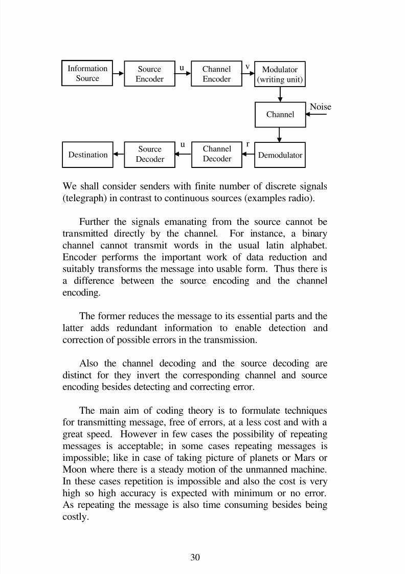
We shall consider senders with finite number of discrete signals
(telegraph) in contrast to continuous sources (examples radio).
Further the signals emanating from the source cannot betransmitted directly by the channel. For instance, a binary
channel cannot transmit words in the usual latin alphabet.
Encoder performs the important work of data reduction andsuitably transforms the message into usable form. Thus there is
a difference between the source encoding and the channel
encoding.
The former reduces the message to its essential parts and the
latter adds redundant information to enable detection and
correction of possible errors in the transmission.
Also the channel decoding and the source decoding are
distinct for they invert the corresponding channel and sourceencoding besides detecting and correcting error.
The main aim of coding theory is to formulate techniquesfor transmitting message, free of errors, at a less cost and with a
great speed. However in few cases the possibility of repeating
messages is acceptable; in some cases repeating messages is
impossible; like in case of taking picture of planets or Mars orMoon where there is a steady motion of the unmanned machine.
In these cases repetition is impossible and also the cost is very
high so high accuracy is expected with minimum or no error.
As repeating the message is also time consuming besides beingcostly.
Information
SourceSource
Encoder Channel Encoder
Modulator
(writing unit)
Channel
Destination Source
Decoder Channel
Decoder Demodulator
Noise
u v
u r

8/2/2019 Erasure Techniques in MRD Codes, by W. B. Vasantha Kandasamy, Florentin Smarandache, R. Sujatha, R. S. Raja …
http://slidepdf.com/reader/full/erasure-techniques-in-mrd-codes-by-w-b-vasantha-kandasamy-florentin-smarandache 32/164
31
We want to find efficient algebraic methods to improve therealiability of the transmission of messages.
In this chapter we give only simple coding and decoding
algorithms which can be easily understood by a beginner.
Binary symmetric channel is an illustration of a model for a
transmission channel. Now we will proceed onto define a linearcode algebraically.
Let x = (x1 … xn) be a code word with k message symbolsand n–k check symbols or control symbols. We know the
message symbols are from Fq, to determine the check symbols.
We obtain the check symbols from the message symbols in such
a way that the code words x satisfy the system of linearequations.
Hxt
= (0), where H is the given n – k × n matrix withelements from Fq.
The standard form for H is (A, In–k ) with A an n – k × k
matrix and In–k the n – k × n – k identity matrix.
The set of all n-dimensional vectors x = (x1, …, xn)
satisfying Hxt
= (0) over Fq is called a linear (block) code C
over Fq of block length n.
The matrix H is called the parity check matrix of the linear(n,k) code C. If q = 2 then we call C a binary code. k/n iscalled transmission (or information) rate.
Since C under addition is a group we call C as a group code.
Also C can be defined as the null space of the matrix H.
We will first illustrate this situation by some examples.
Example 2.1: Let q = 2, n = 7 and k = 4 and C be a C(7, 4) codewith entries from Z2. The message a1, a2, a3, a4 is encoded as the

8/2/2019 Erasure Techniques in MRD Codes, by W. B. Vasantha Kandasamy, Florentin Smarandache, R. Sujatha, R. S. Raja …
http://slidepdf.com/reader/full/erasure-techniques-in-mrd-codes-by-w-b-vasantha-kandasamy-florentin-smarandache 33/164
32
code word x = a1 a2 a3 a4 x5 x6 x7. Here the check symbols are
x5 x6 x7, such that for the given parity check matrix
H =
0 0 1 0 1 1 1
0 1 0 1 1 1 0
1 0 1 1 1 0 0
,
with the set of message symbols from 4
2Z the code words are
given by
0 0 0 0
1 0 0 0
0 1 0 0
0 0 1 0
0 0 0 1
1 1 0 0
1 0 1 0
1 0 0 1
0 1 1 0
0 1 0 1
0 0 1 11 1 1 0
1 1 0 1
1 0 1 1
0 1 1 1
1 1 1 1.
To find C. C = {x ∈ 7
2 Z / Hx
t= (0)}. Hence | C | = 2
4= 16.
Hxt
=
0 0 1 0 1 1 1
0 1 0 1 1 1 0
1 0 1 1 1 0 0
(x1 x2 x3 x4 a5 a6 a7)t
=(0)
gives
C =
{0 0 0 0 0 0 0 1 0 1 0 0 0 1
1 0 0 0 1 1 0 1 0 0 1 0 1 1
0 1 0 0 0 1 1 0 1 0 1 0 0 0
0 0 1 0 1 1 0 1 1 1 0 0 1 0
0 0 0 1 1 0 1 1 0 1 1 1 0 0
1 1 0 0 1 0 1 1 1 0 1 0 0 0
0 1 1 0 1 0 0 0 1 1 1 0 0 1
0 0 1 1 0 1 0 1 1 1 1 1 1 1}
Example 2.2: Take n = 7, k = 4 and q = 2. To construct the
C(7, 4) code using the parity check matrix

8/2/2019 Erasure Techniques in MRD Codes, by W. B. Vasantha Kandasamy, Florentin Smarandache, R. Sujatha, R. S. Raja …
http://slidepdf.com/reader/full/erasure-techniques-in-mrd-codes-by-w-b-vasantha-kandasamy-florentin-smarandache 34/164
33
H =
1 1 1 0 1 0 0
0 1 1 1 0 1 0
0 0 1 1 1 0 1
.
C = {HxT
= (0) where x ∈ 4
2Z }.
C = {0 0 0 0 0 0 0, 1 0 0 0 1 0 1, 0 1 0 0 1 1 1, 0 0 1 0 1 1 0,
0 0 0 1 0 1 1, 1 1 0 0 0 1 0, 1 0 1 0 0 1 1, 1 0 0 1 1 1 0, 0 1 1 0 0
0 1, 0 0 1 1 1 0 1, 0 1 0 1 1 0 0, 1 1 1 0 1 0 0, 1 1 0 1 0 0 1, 1 0 1
1 0 0 0, 0 1 1 1 0 1 0, 1 1 1 1 1 1 1}.
We see the two codes given in examples 2.1 and 2.2 are
C(7, 4) codes but they are different as their parity check matrices are different. Further both the codes have the same set
of message symbols.
Example 2.3: Let C be a (4, 2) code given by the parity check
matrix
H =1 1 1 0
0 1 0 1
.
C = {x ∈ 4
2 Z / Hx
t= (0)}.
= {0 0 0 0, 1 0 1 0, 0 1 1 1, 1 1 0 1}.
Suppose we consider the (4, 2) code using another paritycheck matrix.
H1 =1 0 1 0
1 1 0 1
we get
C = {x ∈ 4
2 Z / H1x
t= (0)}.
= {0 0 0 0, 1 0 1 1, 0 1 0 1, 1 1 1 0}.

8/2/2019 Erasure Techniques in MRD Codes, by W. B. Vasantha Kandasamy, Florentin Smarandache, R. Sujatha, R. S. Raja …
http://slidepdf.com/reader/full/erasure-techniques-in-mrd-codes-by-w-b-vasantha-kandasamy-florentin-smarandache 35/164
34
We see both the codes are different though they have the
same set of message symbols.
We now recall how the repetition code is constructed andthe parity check matrix associated with it. If each code word of
a code consists of only one message symbol x1 ∈ Z2 and n–1check symbols a2 = a3 = … = an are all equal to x1 (x1 is repeatedn–1 times). Thus we obtain a binary (n, 1) code with parity -
check matrix;
H =
1 1 0 ... 0
1 0 1 ... 0
1 0 0 ... 1
.
There are only two code words in this code namely (0 0 …
0) and (1 1 … 1).
This code is used when it impossible and impracticable or
too costly to send original message more than once, liketransmission of information from space crafts or satellites where
it is impossible to use ARQ protocols owing to time limitations.Moving space crafts which takes photos of heavenly bodies is
an example where this code can be used.
Example 2.4: Let C(5, 1) be a binary code obtained from the
parity check matrix;
H =
1 1 0 0 0
1 0 1 0 0
1 0 0 1 0
1 0 0 0 1
. The two code words are 1 1 1 1 1
and 0 0 0 0 0.
Now we proceed onto describe the parity-check code.

8/2/2019 Erasure Techniques in MRD Codes, by W. B. Vasantha Kandasamy, Florentin Smarandache, R. Sujatha, R. S. Raja …
http://slidepdf.com/reader/full/erasure-techniques-in-mrd-codes-by-w-b-vasantha-kandasamy-florentin-smarandache 36/164
35
Parity check code is a (n, n–1) code where we have n–1message symbols and one check symbol. The parity check
matrix is H = (1 1 … 1).
Each code word has only one check symbol and H has onlyeven number of ones.
These codes are used in banking where the last digit of the
account number, usually is a control digit.
Example 2.5: Let H = (1 1 1 1 1 1) be the parity check code. C
is a (6, 5) code and
C ={0 0 0 0 0 0 1 1 1 1 1 1 1 1 0 0 0 0
1 0 0 0 0 1 1 0 1 0 0 0 1 0 0 0 1 0
1 0 0 1 0 0 0 1 1 0 0 0 0 1 0 1 0 00 1 0 0 1 0 0 1 0 0 0 1 0 0 1 1 0 0
0 0 1 0 1 0 0 0 1 0 0 1 0 0 0 1 1 0
0 0 0 1 0 1 0 0 0 0 1 1 1 1 1 1 0 01 1 1 0 1 0 1 1 1 0 0 1 1 1 0 1 1 0
1 1 0 1 0 1 1 1 0 0 1 1 1 0 1 1 1 01 0 1 1 0 1 1 0 1 0 1 1 1 0 0 1 1 10 1 0 1 1 1 0 0 1 1 1 1 1 0 1 1 1 0
0 1 1 1 0 1 0 1 1 1 1 0}
is code associated with the parity check matrix H.
Now we will proceed onto describe the canonical generator
matrix of a linear (n, k) code. Suppose H = (A, In–k ) is the paritycheck matrix associated with the (n, k) code then the generator
matrix G = (Ik – At) is such that GH
T= (0).
Further every code word x = (x1, …, xn) = (a1, …, ak ) G.
We will now describe this situation by some examples.

8/2/2019 Erasure Techniques in MRD Codes, by W. B. Vasantha Kandasamy, Florentin Smarandache, R. Sujatha, R. S. Raja …
http://slidepdf.com/reader/full/erasure-techniques-in-mrd-codes-by-w-b-vasantha-kandasamy-florentin-smarandache 37/164
36
Example 2.6: Let H =
0 1 1 0 1 0 0
1 0 0 1 0 1 0
0 1 1 1 0 0 1
be a parity
check matrix of a C(7, 4) code.
The generator matrix G associated with this (7, 4) code with
the parity check matrix H is given by
G =
1 0 0 0 0 1 0
0 1 0 0 1 0 1
0 0 1 0 1 0 1
0 0 0 1 0 1 1
.
Now using the message symbols from 4
2Z we get the
following code words generated by G.
C = {0 0 0 0 0 0 0, 1 0 0 0 0 1 0, 0 1 0 0 1 0 1, 0 0 1 0 1 0 1,
0 0 0 1 0 1 1, 1 1 0 0 1 1 1, 1 0 1 0 1 0 1, 1 0 0 1 0 0 1, 0 1 1 0 00 0, 0 1 0 1 1 1 0, 0 0 1 1 1 1 0, 1 1 1 0 0 1 0, 0 1 1 1 0 1 1, 1 1 01 1 0 0, 1 0 1 1 1 0 0, 1 1 1 1 0 0 1}.
Example 2.7: Let H =
1 0 1 1 0 0 0
0 1 1 0 1 0 0
1 1 1 0 0 1 0
0 1 0 0 0 0 1
be parity check
matrix associated with a C = C(7, 3) code.
The associated generator matrix
G =
1 0 0 1 0 1 0
0 1 0 0 1 1 1
0 0 1 1 1 1 0
.

8/2/2019 Erasure Techniques in MRD Codes, by W. B. Vasantha Kandasamy, Florentin Smarandache, R. Sujatha, R. S. Raja …
http://slidepdf.com/reader/full/erasure-techniques-in-mrd-codes-by-w-b-vasantha-kandasamy-florentin-smarandache 38/164
37
Now we generate the code,
C = {0 0 0 0 0 0 0, 1 0 0 1 0 1 0, 0 1 0 0 1 1 1, 0 0 1 1 1 1 0,1 0 1 0 1 0 0, 0 1 1 1 0 0 1, 1 1 0 1 1 0 1, 1 1 1 0 0 1 1} is the
code generated by G.
Consider GHT
=
1 0 0 1 0 1 0
0 1 0 0 1 1 1
0 0 1 1 1 1 0
1 0 1 0
0 1 1 1
1 1 1 0
1 0 0 0
0 1 0 0
0 0 1 0
0 0 0 1
=
0 0 0 0
0 0 0 0
0 0 0 0
.
Having seen the generator matrix and parity check matrix of a code we now proceed onto analyse the nature of the generatormatrix.
A generator matrix G for a linear code C is a k × n matrixfor which the rows are a basis of C.
Now a natural question would be what is the purpose of the
parity check matrix H.
We see the parity check matrix serves as the fastest means
to detect errors. So error detection is done by the parity check
matrix. Suppose y is the received code word then find
S(y) = HyT, S (y) is defined as the syndrome. If S(y) = (0) we
say no error and accept y as the correct received word.
If S(y) ≠ (0) we declare error has occurred. Thus the parity
check matrix helps in detecting the error in the received word.So error detection is not a very difficult task as far as coding is

8/2/2019 Erasure Techniques in MRD Codes, by W. B. Vasantha Kandasamy, Florentin Smarandache, R. Sujatha, R. S. Raja …
http://slidepdf.com/reader/full/erasure-techniques-in-mrd-codes-by-w-b-vasantha-kandasamy-florentin-smarandache 39/164
38
concerned. However it is pertinent to mention that when
S(y) = 0, y is a code word, it need not be the transmitted codeword. In certain cases when the error pattern e is identical to a
non zero code word, y is the sum of two code words which is acode word so Hy
T= (0). These errors are not detectable. We
accept them as a correct transmitted message. Thus we have2
k – 1 non zero code words which can lead to undetectable
errors, so we have 2k
– 1 undetectable error patterns. Now the
real problem lies in correcting the error.
We will just describe the coset leader method which is used
to correct errors. Once the error is detected, we know every
code C is a subspace of the vector spacen
qF wheren
qF is
defined over Fq.
The factor spacen
qF / C consists of all cosets a + C = {a + x
| x ∈ C} for any a ∈ n
qF .
Clearly each coset contains qk
vectors as C has 2k
elements
in it. Since a coset is either disjoint or identical we get a
partition onn
qF so
n
qF = C ∪ (a
1+ C) ∪ … ∪ (a
t+ C) for t =
qn–k
–1.
If a vector y is received then y must be an element of one of
these cosets say ai+ C. If the code word x
1has been transmitted
then the error vector e = y – x1 ∈ a
1+ C – x
1= a
1+ C. Thus we
quote the decoding rule [16].
If a vector y is received then the possible error vectors e are
the vectors in the coset containing y. The most likely error isthe vector with minimum weight in the coset of y. Thus y is
decoded as = y – e . The vector of minimum weight in a coset
is called the coset leader. If there are several coset leaders
arbitrarily choose any one of them.
Let a(1), a(2) , …, a(t) be the coset leaders. We have thefollowing table.

8/2/2019 Erasure Techniques in MRD Codes, by W. B. Vasantha Kandasamy, Florentin Smarandache, R. Sujatha, R. S. Raja …
http://slidepdf.com/reader/full/erasure-techniques-in-mrd-codes-by-w-b-vasantha-kandasamy-florentin-smarandache 40/164
39
x(1)
= 0 x(2)
…k (q )
x } code words in C.
a
(1)
+ x
(1)
a
(1)
+ x
(2)
… a
(1)
+
k (q )
x } other cosets
a(t)
+ x(t)
a(t)
+ x(2)
… a(t)
+k (q )
x } other cosets
coset leaders
If a vector y is received then we have to find y in the table.
Let y = a(i)
+ x, then the decoder decides that the error e is
the coset leader a(i). Thus y is decoded as the code word
x = y – e = x(i)
. The code word x occurs as the first element
in the column of y. The coset of y can be found by evaluating
the so called syndrome.
We will illustrate this situation by an example.
Example 2.8: Let C be a binary linear (4, 2) code with the
generator matrix
G =1 0 1 0
0 1 1 1
and parity check matrix
H =1 1 1 0
0 1 0 1
.
The corresponding coset table is
Message symbols 0 0 10 0 1 1 1
Code words 0 0 0 0 1 0 1 0 0 1 1 1 1 1 0 1
Other cosets 1 0 0 0 0 0 1 0 1 1 1 1 0 1 0 10 1 0 0 1 1 1 0 0 0 1 1 1 0 0 1
0 0 0 1 1 0 1 1 0 1 1 0 1 1 0 0
Coset leaders

8/2/2019 Erasure Techniques in MRD Codes, by W. B. Vasantha Kandasamy, Florentin Smarandache, R. Sujatha, R. S. Raja …
http://slidepdf.com/reader/full/erasure-techniques-in-mrd-codes-by-w-b-vasantha-kandasamy-florentin-smarandache 41/164
40
If y = 1 1 1 1 is received then
S (y) =
1
1 1 1 0 1
0 1 0 1 1
1
= (1 0).
Thus error e = 1 0 0 0 and y is decoded as x = y – e =
0 1 1 1 and the corresponding message is 0 1.
Now we will proceed onto define cyclic codes.
We say a code word v in C (C a k dimensional subspace of n
qF ) is a cyclic code if v = (v1 … vn) is in C then (vn v1 … vn-1)
is in C.
We generate cyclic codes using polynomial called the
generator polynomial of a cyclic code.
If g = g0 + g1x + … + gmxm
is a generator polynomial then g / xn
– 1 and deg g = m < n.
Let C be a linear (n, k) code with k = n–m defined by the
generator matrix;
G =
0 1 m
0 m 1 m
0 1 m
g g ... g 0 ... 0
0 g ... g g ... 0
0 ... ... g g ... g
−
=
k 1
g
xg
xg−
.
Then C is cyclic. The rows of G are linearly independent
and rank G = k, the dimension of C.
If xn
– 1 = g1 … gt is a complete factorization of xn– 1 into
irreducible polynomials over Fq then the cyclic codes (gi)generated by polynomials gi are called maximal cyclic codes.

8/2/2019 Erasure Techniques in MRD Codes, by W. B. Vasantha Kandasamy, Florentin Smarandache, R. Sujatha, R. S. Raja …
http://slidepdf.com/reader/full/erasure-techniques-in-mrd-codes-by-w-b-vasantha-kandasamy-florentin-smarandache 42/164
41
A maximal cyclic code is a maximal ideal inq
n
F [x]
x 1⟨ − ⟩.
If g is the polynomial that generates the cyclic code C thenh = x
n–1 / g is defined as the check polynomial of C.
Thus if h = Σ hi xi, hk ≠ 0 then the parity check matrixassociated with the cyclic code C is given by
H =
k 1 0
k k 1 0
k k 1 0
0 0 ... 0 h ... h h
0 0 ... h h ... h 0
. . . . . . . .
h h ... h 0 ... 0 0
−
−
.
We will illustrate this situation by an example.
Example 2.9: Let C = C (7, 4) be a code of length 7 with 4
message symbols and q = 2.
Suppose g(x) = x3
+ x + 1 be the generator polynomial of the cyclic code C. The check polynomial of the cyclic code C is
h = x7–1 / g = x
4+ x
2+ x + 1.
Now the generator matrix
G =
1 1 0 1 0 0 0
0 1 1 0 1 0 0
0 0 1 1 0 1 0
0 0 0 1 1 0 1
and the parity check matrix of this cyclic code is

8/2/2019 Erasure Techniques in MRD Codes, by W. B. Vasantha Kandasamy, Florentin Smarandache, R. Sujatha, R. S. Raja …
http://slidepdf.com/reader/full/erasure-techniques-in-mrd-codes-by-w-b-vasantha-kandasamy-florentin-smarandache 43/164
42
H =
0 0 1 0 1 1 1
0 1 0 1 1 1 0
1 0 1 1 1 0 0
.
Now we can generate the cyclic code using G. aG = x
where a is the message from 4
2Z and x the resulting code word
of C. We have referred and information are from [1, 16].
Now we proceed onto just recall the definition of rank
distance codes and give some of the properties related with
them.
Error detection, error correction for these linear block codes
can be found in [1, 6, 16, 18]. However the erasure techniquesfor these codes are very meagre hence we just describe the
erasure techniques in these codes.
When the code symbols are from the Galois field GF(2n) of
an arbitrary dimension the function of the modulator is to matchthe encoder output to the signals of the transmission channel.
The modulator accepts the binary encoded symbols and
produces wave forms or signals appropriate to the physical
transmission medium. At the receiving end of thecommunication link, the demodulator operates on the signals
received from a separate transmission symbol interval or a set of
elements in {0, 1}. The demodulator is designed to make a
definite decision for each received symbol 0 or 1.
The definition of a channel includes the modulator, thedemodulator and all intervening transmission equipment and
media. Most of them are discrete memoryless channel. The
assumption is made in that the output symbol at any instant of
time depends statistically only on the input symbol at that time.

8/2/2019 Erasure Techniques in MRD Codes, by W. B. Vasantha Kandasamy, Florentin Smarandache, R. Sujatha, R. S. Raja …
http://slidepdf.com/reader/full/erasure-techniques-in-mrd-codes-by-w-b-vasantha-kandasamy-florentin-smarandache 44/164
43
The coding system is described by the following figure.
↓
↓
↓
↓
↓
↓
This simple model [20] is known as the binary symmetricchannel and is described in the following figure.
In this model the modulator input x has value 0 or 1 and the
demodulator output y has value 0 or 1. When 0 is transmittedand 1 is received the error probability is p. When 0 is
transmitted and 0 is received the probability is 1 – p. Similarly
when 1 is transmitted and 0 is received the probability is p andwhen 1 is transmitted and 1 is received the probability is 1 – p.
This model can be described simply as a binary-input and
binary-output model.
• 0 • 0 0 • • 0p 1–p
• 1 • 1 1 • • 1
Sender
encoder
modulator
channel
demodulator
decoder
receiver
corrected message
message

8/2/2019 Erasure Techniques in MRD Codes, by W. B. Vasantha Kandasamy, Florentin Smarandache, R. Sujatha, R. S. Raja …
http://slidepdf.com/reader/full/erasure-techniques-in-mrd-codes-by-w-b-vasantha-kandasamy-florentin-smarandache 45/164
44
• 0 • 0 0 • • 0
p• 1 • 1 1 • • 1
1–p
0 • • 0
1 • • 1
Binary symmetric channel
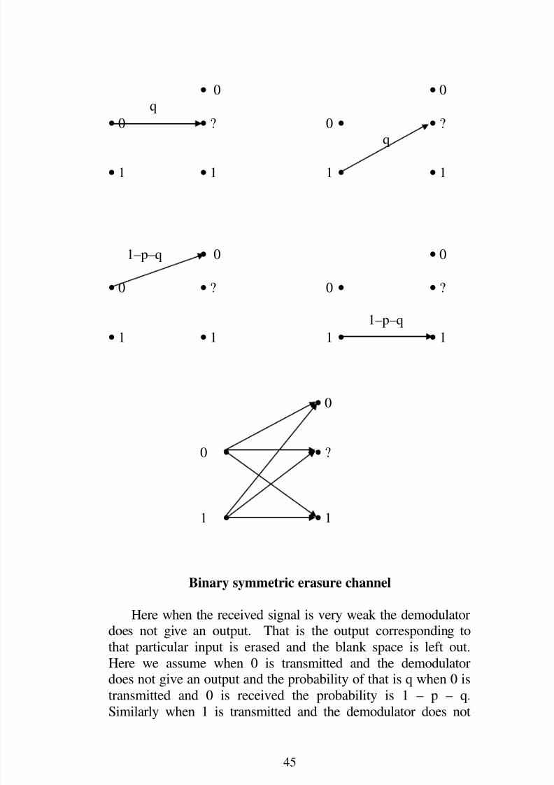
When erasure occurs [20] has studied the binary symmetricerasure channel. This channel model is depicted in the
following figure which includes a symmetric transmission from
either input symbol to an output symbol labeled ‘?’ to denoteambiguity. Now when an input symbol is sent we have thethree possibilities.
(i) The correct output is received.(ii) An erroneous output is received.
(iii) The demodulator is unable to decide, the result
is a blank space, that is ambiguous.
• 0 • 0
• 0 • ? 0 • p • ?
p
• 1 • 1 1 • • 1
8/2/2019 Erasure Techniques in MRD Codes, by W. B. Vasantha Kandasamy, Florentin Smarandache, R. Sujatha, R. S. Raja …
http://slidepdf.com/reader/full/erasure-techniques-in-mrd-codes-by-w-b-vasantha-kandasamy-florentin-smarandache 46/164
45
• 0 • 0q
• 0 • ? 0 • • ?
q
• 1 • 1 1 • • 1
1–p–q • 0 • 0
• 0 • ? 0 • • ?
1–p–q
• 1 • 1 1 • • 1
• 0
0 • • ?
1 • • 1
Binary symmetric erasure channel
Here when the received signal is very weak the demodulatordoes not give an output. That is the output corresponding to
that particular input is erased and the blank space is left out.
Here we assume when 0 is transmitted and the demodulatordoes not give an output and the probability of that is q when 0 is
transmitted and 0 is received the probability is 1 – p – q.
Similarly when 1 is transmitted and the demodulator does not

8/2/2019 Erasure Techniques in MRD Codes, by W. B. Vasantha Kandasamy, Florentin Smarandache, R. Sujatha, R. S. Raja …
http://slidepdf.com/reader/full/erasure-techniques-in-mrd-codes-by-w-b-vasantha-kandasamy-florentin-smarandache 47/164
46
give a output the probability is q. When 1 is transmitted and the
modulator does not give an output the probability is p. When 1is transmitted and 1 is received the probability is 1 – p – q.
The outputs that are erased by the demodulator are called
erasures or blank spaces [6-8]. Thus when erasures are presentin the received code word those coordinates received in the code
word would be blank spaces.
The study of properties of erasures out weighs the study of
properties of errors in a code as we are sure of the number of
errors that has occurred by counting the number of blank spaces(erasures) and we are also aware of their locations as they are
blank during the transmission process.
But if are to study only errors we may not completely becertain of the number of errors occurred during the
transmission, for instance when a message is sent and the
received message is also a code word different from the sentmessage, we may not be able to determine it as error but in case
of erasures it may be blank.
Another advantage of erasure techniques over the study of
error is that even a lay man can guess that the received message
is an erroneous one. Also we can say whether the original
message is retrievable or not. The study of erasures in case of Hamming metric has been widely studied by [21-2] and [6-8].
We would be defining the new notion of “blanks” which arenot erasures. These ‘blanks’ will be known as “special blanks”
and we will not be using the notion of erasure decoding we use
only the error decoding technique. We will use this “special
blank” notion in the last chapter of this book where we will beusing them in concatenation of linear coding with Hamming
metric defined on it.
Now refer Gabidulin for the notion of rank distance codes.

8/2/2019 Erasure Techniques in MRD Codes, by W. B. Vasantha Kandasamy, Florentin Smarandache, R. Sujatha, R. S. Raja …
http://slidepdf.com/reader/full/erasure-techniques-in-mrd-codes-by-w-b-vasantha-kandasamy-florentin-smarandache 48/164
47
DEFINITION 2.1: Let X n
be a n-dimensional vector space over
the field GF(2 N
). Let u1 , u2 , …, un be a fixed basis for X n
over
GF(2 N
). Then any element x ∈ X n
can be represented as a n-
tuple (x1 , x2 , …, xn) where xi ∈ GF(2 N ) (1 ≤ i ≤ n).
GF(2 N
) is a vector space of dimension N over GF(2). Let
v1 , v2 , …, v N be a fixed basis for GF(2 N
) over GF(2). Then any
element xi ∈ GF(2 N
) can be uniquely represented in the form of
a N-tuple (m1i , m2i , …, m Ni),n
N M denote the ensemble of all
(N × n) matrices with elements from GF(2).
Consider the bijection M : X n → nNM defined by the
following condition for any vector x = (x1 , x2 , …, xn) ∈ X n; the
associated matrix;
M (x) =
11 12 1n
21 22 2n
N 1 N 2 Nn
m m ... m
m m ... m
m m ... m
where the ith
column represents the ith
coordinate xi of x over
GF(2).
The rank of a vector x ∈ X n
over GF(2) is defined as the
rank of the matrix M(x) over GF(2). Let r(x) denote the rank of
the vector x ∈ X n
over GF(2). By the properties of the rank of a
matrix the mapping x → r(x) defines a norm on X n
; called therank norm.
Let X n
be a vector space of dimension n over GF(2n)
equipped with the rank norm. Clearly the rank norm induces a
metric defined as the rank metric (rank distance) on X n
and is
denoted by d R. For x, y ∈ X n , the rank distance between x and y
is d R(x, y) = r (x–y). A vector space X n
over GF(2n) such that
n≤
N equipped with the rank metric d R is defined as a rank distance space. So if X n
is a rank distance space, a linear (n, k)

8/2/2019 Erasure Techniques in MRD Codes, by W. B. Vasantha Kandasamy, Florentin Smarandache, R. Sujatha, R. S. Raja …
http://slidepdf.com/reader/full/erasure-techniques-in-mrd-codes-by-w-b-vasantha-kandasamy-florentin-smarandache 49/164
48
rank distance code is a linear subspace of dimension k in the
rank distance space X n
and is denoted by C.
A generator matrix G of C is a k × n matrix with entries from GF(2
N ) whose rows form a basis for C.
Then a (n – k) × n matrix H with entries from GF(2 N
) such
that GH T
= (0) is called the parity check matrix of C where (0)
denotes a k × n – k zero matrix.
Suppose C is a (n, k) rank distance code with generator
matrix G and parity check matrix H then C is the row space of G or the null space of H. We have minimum distance of C
defined as d = min {r(x – y) : x, y ∈ C; x ≠ y}. C is a k -
dimensional subspace of the rank distance space Xn, if x, y ∈ C
then x – y ∈ C.
Hence d the minimum distance,
d = min {r(x) | x ∈ C; x ≠ 0}. The notion of maximum rank and the erasure techniques would be studied in the following
chapters.

8/2/2019 Erasure Techniques in MRD Codes, by W. B. Vasantha Kandasamy, Florentin Smarandache, R. Sujatha, R. S. Raja …
http://slidepdf.com/reader/full/erasure-techniques-in-mrd-codes-by-w-b-vasantha-kandasamy-florentin-smarandache 50/164
49
Chapter Three
ERASURE DECODING OF MAXIMUM R ANK
DISTANCE CODES
This chapter has three sections. Section one is introductory in
nature. In section two we describe the class of MRD codes as
given by E.M. Gabidulin [9]. In section three we discuss thesystematic guessing process or filling up of the blank spaces in
case of erasures for MRD codes [17, 29, 32]. 3.1 Introduction
Algebraic coding theory is required in communication
systems to combat the errors that occur during transmission. Inmany communication systems, it is often convenient to
represent the set of signals to be transmitted as a higher
dimensional Galois field. There are many reasons to do so.
One is that it makes it possible to visualize the signals by meansof vectors, which in turn has the advantage of recognizing the
relationship among various types of signals that is to be
considered. Secondly, the length of the message will be verymuch reduced resulting an increase in the rate of transmission.
Here the set of basic signals will be represented by a prime
Galois field GF(p) and all the possible linear combinations of

8/2/2019 Erasure Techniques in MRD Codes, by W. B. Vasantha Kandasamy, Florentin Smarandache, R. Sujatha, R. S. Raja …
http://slidepdf.com/reader/full/erasure-techniques-in-mrd-codes-by-w-b-vasantha-kandasamy-florentin-smarandache 51/164
50
the basic signals will be represented by a higher dimensional
Galois field, GF(pn).
When the code symbols are from a higher dimensionalGalois field the function of the modulator is to match the
encoder output to the transmission channel. A definition of achannel generally includes the modulator, the demodulator and
all the intervening transmission equipment and media. In this
model in certain situations, for example when the receivedsignal is very weak the demodulator does not give an output.
That is, the output corresponding to that particular input is
erased and a black space of left out.
The outputs that are erased by the demodulator are called
erasures or blank spaces. Hence the events in which the
demodulator does not give a output when the evidence does notclearly indicate one signal as the most probable are called
erasures. Hence when erasures are present in the received
vector those coordinates in the received vector will be blank spaces. Erasure decoding in case of Hamming metric has been
widely studied by W.W. Peterson [21-2], David Forney [6-8].Here we obtain a method of erasure decoding for the class of MRD codes when the minimum distance is same as the length
of the code. The error correcting capability of the MRD code
depends on the minimum distance and greater the minimum
distance greater the error correcting capability. In this chapterthe minimum distance of the MRD code is equal to its length.
By making use of this systematic guessing process anerasure or blank space can be regarded as an error which can
either be detected or corrected by making use of the decoding
algorithm for MRD codes. We have proved that a MRD code of
length n, dimension 1 and minimum distance n = 2t + 1 cancorrect atmost t erasures and detect more than t erasures. We
have obtained the number of ways in which a particular erasure
can be chosen during the guessing process and we haveestablished that the result is unaffected by various choices for
the erasures available during the guessing process at each stage.

8/2/2019 Erasure Techniques in MRD Codes, by W. B. Vasantha Kandasamy, Florentin Smarandache, R. Sujatha, R. S. Raja …
http://slidepdf.com/reader/full/erasure-techniques-in-mrd-codes-by-w-b-vasantha-kandasamy-florentin-smarandache 52/164
51
Also the method of erasure decoding is illustrated through an
example.
3. 2 Maximum Rank Distance Codes
Maximum Rank Distance (MRD) codes are a class of codes
which are analogs of generalized Reed-Solomon codes [26].
MRD codes are codes of length n < N defined over GF(2N)
equipped with the rank metric.
Suppose Xn
is a n-dimensional vector space over the field
GF(2N). Let u1, u2, …, un be a fixed basis for X
nover GF(2
N).
Then any element x ∈ Xn
can be represented as an n-tuple (x1,
x2, …, xn) where xi ∈ GF(2N).
GF(2N) is a vector space of dimension N over GF(2). Let
v1, v2, …, vN be a fixed basis for GF(2N) over GF(2). Then any
element xi ∈ GF(2N) can be uniquely represented in the form of
a N-tuple (a1i, a2i, …, aNi). Let n
NA denote the ensemble of all
(N×
n) matrices with elements from GF(2).
Consider the bijection A : Xn → n
NA defined by the
following rule:
For any vector x = (x1, x2, …, xn) ∈ Xn
the associated matrix
A(x) =
11 12 1n
21 22 2n
N1 N2 Nn
a a ... a
a a ... a
a a ... a
(3.2.1)
where the ith
column represents the ith
coordinate ‘xi’ of ‘x’ over
GF(2). We recall some of the basic definition from [9, 29, 30,32].
DEFINITION 3.2.1: The rank of a vector x ∈ X n
over GF(2) is
defined as the rank of the matrix A(x) over GF(2). In other
words the rank of a vector x ∈ X n
is the maximum number of

8/2/2019 Erasure Techniques in MRD Codes, by W. B. Vasantha Kandasamy, Florentin Smarandache, R. Sujatha, R. S. Raja …
http://slidepdf.com/reader/full/erasure-techniques-in-mrd-codes-by-w-b-vasantha-kandasamy-florentin-smarandache 53/164
52
columns that are linearly independent over GF(2) in the
associated matrix A(x) of the vector x. Let r(x) denote the rank
of the vector x ∈ X n
over GF(2). By the properties of the rank
of a matrix the mapping x r (x) specifies a norm on X n and iscalled the rank norm.
DEFINITION 3.2.2: Let X n
be a vector space of dimension n
over GF(2 N
) equipped with rank norm. The rank norm induces
a metric defined as the rank metric (rank distance) on X n
and is
denoted by d R. For x, y ∈ X n
the rank distance between x and y
is d R (x, y) = r (x–y).
DEFINITION 3.2.3: A vector space X n
over GF(2 N
) such that
n < N equipped with the rank metric d R is defined as a rank
distance space.
DEFINITION 3.2.4: Let X n
be the rank distance space. A linear
(n, k) rank distance code is a linear subspace of dimension k in
the rank distance space X n
and is denoted by C.
DEFINITION 3.2.5: Let C be a linear (n, k) rank distance code. A generator matrix G of C is a k × n matrix with entries from
GF(2 N
) whose rows form a basis for C.
DEFINITION 3.2.6: Let C be a linear (n, k) rank distance code
with generator matrix G. Then a (n – k) × n matrix H with
entries from GF(2 N
) such that GH T
= (0) is called the parity
check matrix of C where (0) denotes the k × (n – k) zero matrix.
Suppose C is a linear (n, k) rank distance code withgenerator matrix G and parity check matrix H, then C can be
thought of as :
1. the row space of G or
2. the null space of H.
DEFINITION 3.2.7: Let C be a linear (n, k) rank distance code.
The minimum distance of C is defined as d = min {r (x – y) : x, y

8/2/2019 Erasure Techniques in MRD Codes, by W. B. Vasantha Kandasamy, Florentin Smarandache, R. Sujatha, R. S. Raja …
http://slidepdf.com/reader/full/erasure-techniques-in-mrd-codes-by-w-b-vasantha-kandasamy-florentin-smarandache 54/164
53
∈ C, x ≠ y}. Since C is linear space, d is also equal to min {r(x)
: x ∈ C, x ≠ 0}.
A linear (n, k) rank distance code C with minimum distance
d satisfies the following bound.
Singleton-style bound[12, 16]: A linear (n, k) rank distance code
C with minimum distance d satisfies the inequality d ≤ n–k+1.
DEFINITION 3.2.8: Rank distance codes which attain equality
in the singleton style bound are called Maximum Rank Distance
codes (MRD codes).
MRD codes are analogs of generalized Reed-Solomoncodes and can be defined through generator and parity check
matrices. A MRD code with length n = N can be defined as
follows:
Let [i] = 2i, i = 0, ± 1, ± 2, …
Let hi ∈ GF(2N), i = 1, 2, …, n be linearly independent over
GF(2).
For a given design distance d < n let us generate the matrix
H =
1 2 n
[1] [1] [1]
1 2 n
[d 2] [d 2] [d 2]
1 2 n
h h ... h
h h ... h
h h ... h− − −
(3.2.2)
The linear (n, k) rank distance code with parity check
matrix H given in equation (3.2.2) is an MRD code of length nand minimum distance d. We denote a (n, k, d) MRD code as
C[n, k].
The encoding and decoding algorithm for MRD codes are
given by Gabidulin [9].

8/2/2019 Erasure Techniques in MRD Codes, by W. B. Vasantha Kandasamy, Florentin Smarandache, R. Sujatha, R. S. Raja …
http://slidepdf.com/reader/full/erasure-techniques-in-mrd-codes-by-w-b-vasantha-kandasamy-florentin-smarandache 55/164
54
3.3 Erasure Decoding of MRD codes
It has long been recognized that there are advantages in
allowing the demodulator not to guess at all on certaintransmission (for example when the received signal is veryweak) when the evidence does not clearly indicate one signal as
the most probable: such events are called erasures. In the event
of an erasure or blank space it is convenient to passes on the
side information to the decoder that this guess is not completelyreliable. By the guessing process or filling up of the blank
space an erasure or blank space can be regarded as an error
which can be either detected or corrected by making use of thedecoding algorithm for MRD codes.
The guessing process or filling up of the blank spaces canbe done systematically by making use of the decoding
properties of the MRD codes and this procedure is described
below.
The C[n, 1] be a (n, 1, n) MRD code defined over GF(2n),
where n = 2t + 1. Since the minimum distance of this code is nthe associated matrix of every code word in this code has ncolumns to be linearly independent over GF(2).
Suppose x = (x1, x2, …, xn) is the codeword that istransmitted. Let y = (y1, y2, …, yn) be the received vector where
t coordinates are erasures. Let *1, *2, …*t denote the t erasures.
The t erasures can occur either in an array or can occur
intermittently with the yi’s or it can be randomly placed inbetween the yi’s. Still the method adopted by us will not affect
the result. Without loss of generality we can assume that *1, *2,
…, *t be the first t coordinates of y. Let yt+1, yt+2, …yn be therest of the n – t coordinates. The choosing of each of the * j’s for
j = 1, 2, …, t is detailed below.
Now choose *1 (*1 ≠ 0) such that the set {*1, yt+1, yt+2, …,yn} is a linearly independent set over GF(2). Having chosen *1,
now choose *2 (*2 ≠ 0) such that the set (*2, *1, yt+1, yt+2, …, yn)is a linearly independent set over GF(2). Having chosen *1, *2,

8/2/2019 Erasure Techniques in MRD Codes, by W. B. Vasantha Kandasamy, Florentin Smarandache, R. Sujatha, R. S. Raja …
http://slidepdf.com/reader/full/erasure-techniques-in-mrd-codes-by-w-b-vasantha-kandasamy-florentin-smarandache 56/164
55
…, *s, s < t, *s+1 is chosen such that *s+1 ≠ 0 and the set {*s+1, *1,*2,… , *s, yt+1, yt+2, …, yn} is linearly independent over
GF(2).
By the above guessing process or filling up of the blank
spaces the t erasures *1, *2, …, *t in the received vector y are
filled by the t probable errors. Let the vector y′ = ( 1 2 ny , y ,..., y′ ′ ′ )
be the vector obtained from y after converting the t erasures or tblank spaces into t errors by using the guessing process. Now
we apply the decoding algorithm of the MRD codes for
decoding y′ and obtain the correct message transmitted.
The following theorem gives the number of ways in whichthe erasures or blank spaces can be chosen by using the
guessing process or filling up of the blank spaces.
THEOREM 3.3.1: Let C[n,1] be a (n, 1, n) MRD code defined
over GF(2n) where n=2t + 1. Let x = (x1 , x2 , …, xn) be the
transmitted code word. Let y = (y1 , y2 , …, yn) be the received
vector where t coordinates are erasures or blank spaces. Let *1 ,
*2 , …, *t denote the t erasures or t blank spaces. Then *s+1 ,
where s + 1 < t can be chosen in 2n–t+2
[2t–s
– 1] ways by using
the guessing process.
Proof: Let C[n, 1] be a MRD (n, 1, n) code defined over
GF(2n) where n = 2t + 1. Suppose x = (x1, x2, …, xn) is the
codeword that is transmitted. Let y = (y1, y2, …, yn) be the
received vector where t coordinates are erasures or blank
spaces.
Let *1, *2, …, *t denote the t erasures or blank spaces.
Without loss of generality let *1, *2, …, *t be the first
coordinates of the vector y. Then when applying the guessing
process *1 is chosen such that *1 ≠ 0 and the set {*1, yt+1, yt+2,…, yn} is a linearly independent set over GF(2). That is, *1 is
chosen from the set B1 = GF(2n) \ {0, yt+1, …, yn, yt+1 + yt+2, …,
yn–1 + yn, yt+1 + yt+2 + yt+3, …, yn–2 + yn–1 + yn, …, yt+1 + yt+2 + …
+ yn–1 + yn}.

8/2/2019 Erasure Techniques in MRD Codes, by W. B. Vasantha Kandasamy, Florentin Smarandache, R. Sujatha, R. S. Raja …
http://slidepdf.com/reader/full/erasure-techniques-in-mrd-codes-by-w-b-vasantha-kandasamy-florentin-smarandache 57/164
56
Hence *1 can be chosen in |B1| ways, where |B1| denotes the
number of elements in the set B1. Clearly
|B1| = 2n
– (1 + n – tC1 + n – tC2 + n – tC3 + … + n – tCn–t–1 + n – tCn–1)
= 2n
– (1+1)n–1
(by Binomial theorem)= 2
n– 2
n–t
= 2n–t
[2t– 1].
Having chosen *1, *2 can be chosen such that *2 ≠ 0 and theset {*2, *1, yt+1, yt+2, …, yn} is linearly independent over GF(2).
That is, *2
is chosen from the set
B2 = GF(2n) \ {0,*1, yt+1, …, yn, *1 + yt+1, yt+1 + yt+2, …, yn–1
+ yn, *1 + yt+1 + yt+2, yt+1+ yt+2 + yt+3, …, yn–2 + yn–1 + yn, …, *1 +
yt+1 + yt+2 + … + yn–1 + yn}. Hence *2 can be chosen in |B2|
ways. Clearly |B2| is given by;
|B2| = 2n
– (1 + n – (t+1)C1 + n – (t+1)C2
+ … + n – (t+1)Cn–t + n – (t+1)Cn–t+1)
= 2n
– (1+1)n–t+1
(By binomial theorem)
= 2n
– 2n–t+1
= 2n–t+1
[2t–1
– 1].
Having chosen *1, *2,..., *s, s < t, *s+1 is chosen such that
*s+1 ≠ 0 and {*s+1, *1, *s, …, *s, yt+1, yt+2, …, yn} is linearlyindependent set over GF(2). Hence *s+1 can be chosen in |Bs+1|
ways. Clearly |Bs+1| is
|Bs+1| = 2n
– (1 + n – (t+s)C1 + n – (t+s)C2 + n – (t+s)C3
+ … + n – (t+s)Cn–t+s–1 + n – (t+s)Cn–t+s)
= 2n
– (1+1)n–t+s
= 2n
– 2n–t+s
= 2n–t+s
[2t–s
– 1].
Hence the theorem.

8/2/2019 Erasure Techniques in MRD Codes, by W. B. Vasantha Kandasamy, Florentin Smarandache, R. Sujatha, R. S. Raja …
http://slidepdf.com/reader/full/erasure-techniques-in-mrd-codes-by-w-b-vasantha-kandasamy-florentin-smarandache 58/164
57
THEOREM 3.3.2: Let C[n, 1] be a (n, 1, n) MRD code with
minimum distance n = 2t + 1. Then C[n, 1] corrects atmost t
ensures and detects more than t erasures.
Proof: Let C [n, 1] be a (n, 1, n) MRD code with minimum
distance n = 2t + 1. Suppose x = (x1, x2, …, xn) is the codewordthat is transmitted. Let y = (y1, y2, …, yn) be the received vector
where t coordinates are erasures or blank spaces. Let y′ =
( 1 2 ny , y ,..., y′ ′ ′ ) be the vector obtained from y after converting the
t erasures into t errors by using the guessing process or filling
up of the blank spaces. Therefore, dR (x, y′) < t, by [9, 29, 30]
we know that a MRD code with n = 2t + 1 can correct atmost terrors and detect more than t errors. Hence C[n, 1] can correct
atmost t erasures and detect more than t erasures.
THEOREM 3.3.3: Let C[n, 1] be a (n, 1, n) MRD code defined
over GF(2n) where n = 2t + 1. Let x = (x1 , x2 , …, xn) be the
transmitted codeword. Let y = (y1 , y2 , …, yn) be the received
vector where t coordinates are erasures. Let *1 , *2 , …, *t
denote the t erasures. The erasures *s+1 , where s + 1 ≤ t can be
chosen in 2n–t+s [2t–s –1] ways by using the guessing process.
Then the various choices of * j’s does not affect the erasure
correcting capability of the MRD code.
Proof : Let C[n, 1] be a (n, 1, n) MRD code defined over
GF(2n) where n = 2t + 1. Suppose x = (x1, x2, …, xn) be the
transmitted codeword. Let y = (y1, y2, …, yn) be the receivedvector where t coordinates are erasures or blank spaces. Let *1,
*2,…, *t denote the t erasures or t blank spaces. Lety′ = ( 1 2 ny , y ,..., y′ ′ ′ ) be the vector obtained from y after applying
the guessing process or filling up of the blank spaces to obtainfrom y after applying the guessing process or filling up of the
blank spaces to the received vector y. Let y″ = ( 1 2 ny ,y ,...., y′′ ′′ ′′ )
be another vector obtained from y after applying the guessing
process or filling up of the blank spaces to the received vector y
and be such that y′ ≠ y″ , then dR(y′, y″ ) ≤ t. By the guessing
process the t erasures in the received vector y are converted intot errors. Hence dR(x, y′) ≤ t and dR(x, y″ ) ≤ t. We know MRD

8/2/2019 Erasure Techniques in MRD Codes, by W. B. Vasantha Kandasamy, Florentin Smarandache, R. Sujatha, R. S. Raja …
http://slidepdf.com/reader/full/erasure-techniques-in-mrd-codes-by-w-b-vasantha-kandasamy-florentin-smarandache 59/164
58
code with n = 2t + 1 can correct atmost t errors and detect more
than t errors. Since dR(x, y′) ≤ t and dR(x, y″ ) ≤ t both the vector
y″ and y′ are both decoded as the vector x, which is the
transmitted message. Hence the theorem.
The guessing process and the above results are illustrated by
the following example.
Example 3.3.1: Consider GF(23) where GF(2
3) = {0, 1, α, α
2,
…, α6} and α is the root of the primitive polynomial p(x) = x
3+
x + 1. Consider the (3, 1, 3) MRD code having parity check
matrix H.
H =2
2 4
1
1
α α
α α (3.3.1)
obtained by choosing h1 = 1, h2 = α, h3 = α2
in the matrix(3.3.1).
Let m1 = α5
be the message. Let x = (α5, a1, a2). The Hx
T=
(0) gives a1 = α6 and a2 = α2. The codeword corresponding tothe message m1 = α
5is c = (α
5, α
6, α
2). Suppose c is the
transmitted vector and let y = (α5, *, α
2) be the received vector
with one erasure or one blank space. By applying the guessing
process we choose * ≠ 0 and such that the set {*, α5, α
2} is
linearly independent over GF(2). Then there are four choices
for * namely * = 1, * = α, * = α4
and * = α6. We see that the
choice of * does not change the result and we get the corrected
message for all the four choices of *.
Choose * = 1.
Now the vector y′ obtained after filling up of the blank
space in the received vector y is y′ = (α5,1, α
2). By applying the
decoding algorithm for MRD codes to the vector y′ we have
1. Syndrome = (α
3
,α
4
) = (s0, s1).

8/2/2019 Erasure Techniques in MRD Codes, by W. B. Vasantha Kandasamy, Florentin Smarandache, R. Sujatha, R. S. Raja …
http://slidepdf.com/reader/full/erasure-techniques-in-mrd-codes-by-w-b-vasantha-kandasamy-florentin-smarandache 60/164
59
2. ∆ (z) = α2z + z
2.
3. The non zero root of ∆ (z) is E1 = α2.
4. Solving sp =1
[p]
j j
j 1
E x=
∑ , p = 0 we get x1 = α .
5. Solving x1 =3
1j j
j 1
Y h=
∑ gives Y11 = 0, Y12 = 1,
Y13 = 0 and hence the matrix Y = (0 1 0).
6. Error vector e = E1 Y = (0, α2, 0).
7. y′ + e = (α5, α
6, α
2) is the required codeword.
Choose * = α.
Now the vector y′ obtained after filling up of the blank
space in the received vector y is y′ = (α5, α, α
2). By applying
the decoding algorithm for MRD codes to the vector y′ we have
1 Syndrome = (α6,1) = (s0, s1).
2. ∆ (z) = α5z + z
2.
3. The non zero root of ∆ (z) is E1 = α5.
4. Solving sp =1
[p]
j j
j 1
E x=
∑ , p = 0 we get x1 = α .
5. Solving x1 =3
1j j
j 1
Y h=
∑ gives Y11 = 0, Y12 = 1,
Y13 = 0 and hence the matrix Y = (0 1 0).
6. Error vector e = E1 Y = (0, α5, 0).

8/2/2019 Erasure Techniques in MRD Codes, by W. B. Vasantha Kandasamy, Florentin Smarandache, R. Sujatha, R. S. Raja …
http://slidepdf.com/reader/full/erasure-techniques-in-mrd-codes-by-w-b-vasantha-kandasamy-florentin-smarandache 61/164
60
7. y′ + e = (α5, α
6, α
2) is the required codeword.
Choose * = α4.
Now the vector y′ obtained after filling up of the blank
space in the received vector y is y′ = (α5, α
4, α
2). By applying
the decoding algorithm for MRD codes to the vector y′ we have
Syndrome = (0, 0).
This indicates that y′ is the correct message.
Let m2 = α3
be the message. Let x = (α3, a1, a2). The Hx
T=
(0) gives a1 = α4
and a2 = 1 . The codeword corresponding to
the message m1 = α3
is c = (α3, α
4, 1). Suppose c is the
transmitted vector and let y = (α3, *1, *2) be the received vector
with two erasures or blank spaces. By applying the guessing
process we choose *1 ≠ 0 and such that the set {*1, α3} is
linearly independent over GF(2). Since the set {α6, α
3} is
linearly independent over GF(2) choose *1 = α
6
. Again sincethe set {α
2, α
6, α
3} is a linearly independent set over GF(2)
choose *2 = α2. Now the vector y′ obtained after filling up of
the blank spaces in the received vector y is y′ = {α3, α
6, α
2}.
By applying the decoding algorithm for MRD codes to the
vector y′ we have
1. Syndrome = (α
4
,α
5
) = (s0, s1).
2. ∆ (z) = α3z + z
2.
3. The nonzero root of ∆ (z) is E1 = α3.
4. Solving sp =1
[p]
j j
j 1
E x=
∑ , p = 0 we get x1 = α .

8/2/2019 Erasure Techniques in MRD Codes, by W. B. Vasantha Kandasamy, Florentin Smarandache, R. Sujatha, R. S. Raja …
http://slidepdf.com/reader/full/erasure-techniques-in-mrd-codes-by-w-b-vasantha-kandasamy-florentin-smarandache 62/164
61
5. Solving x1 =3
1j j
j 1
Y h=
∑ gives Y11 = 0, Y12 = 1,
Y13
= 0 and hence the matrix Y = (0 1 0).
6. Error vector e = E1 Y = (0, α3, 0).
8. y′ + e = (α5, α
6, α
2) is the required codeword.
Choose * = α6.
Now the vector y′ obtained after filling up of the blank
space in the received vector y is y′ = (α5, α6, α2). By applying
the decoding algorithm for MRD codes to the vector y′ we have
Syndrome = (0, 0).
This indicates that y′ is the correct message.
Let m2 = α3
be the message. Let x = (α3, a1, a2). The Hx
T=
(0) gives a1 = α4 and a2 = 1 . The codeword corresponding tothe message m1 = α
3is c = (α
3, α
4, 1). Suppose c is the
transmitted vector and let y = (α3, *1, *2) be the received vector
with two erasures or two blank space. By applying the guessing
process we choose *1 ≠ 0 and such that the set {*1, α3} is
linearly independent over GF(2). Since the set {α6, α
3} is
linearly independent over GF(2) choose *1 = α6. Again since
the set {α2, α
6, α
3} is a linearly independent set over GF(2)
choose *2 = α2
. Now the vector y′ obtained after filling up of the blank spaces in the received vector y is y′ = {α
3, α
6, α
2}.
By applying the decoding algorithm for MRD codes to the
vector y′ we have
1. Syndrome = (α2, α
2) = (s0, s1).
2. ∆ (z) = α
2
z + z
2
.

8/2/2019 Erasure Techniques in MRD Codes, by W. B. Vasantha Kandasamy, Florentin Smarandache, R. Sujatha, R. S. Raja …
http://slidepdf.com/reader/full/erasure-techniques-in-mrd-codes-by-w-b-vasantha-kandasamy-florentin-smarandache 63/164
62
3. The nonzero root of ∆ (z) is E1 = α2.
4. Solving sp =
1[p]
j j j 1 E x=∑ , p = 0 we get x1 = 1 .
5. Solving x1 =3
1j j
j 1
Y h=
∑ gives Y11 = 1, Y12 = 0,
Y13 = 0 and hence the matrix Y = (1 0 0).
Error detected.
The erasure decoding method declares that more than oneerasure has been detected.
Hence the (3, 1, 3) MRD code corrects atmost one erasureand detects more than one erasure in the received vector. We
also note that the result is independent of the choice of *.
The study of erasure decoding is better than the study of
errors. Erasure decoding in case of Hamming codes has beenwidely studied in literature. In this chapter we have started the
study of erasure decoding of the class of MRD codes. We givea guessing process by which the erasures or blank spaces in the
received vector can be converted into errors. We have proved
that the MRD code of length n, dimension one and minimumdistance n = 2t + 1 can correct atmost t erasures and detect more
than t erasures. We have obtained the number of ways in which
a particular erasure can be chosen during the guessing process
and we have established that the result is unaffected by thevarious choices of erasures or blank spaces that are available in
the guessing process or filling up of the blank spaces at each
stage.
It is pertinent to mention that these results are true for any
(n, k, d) MRD code defined over GF(2n) where d = 2t + 1.

8/2/2019 Erasure Techniques in MRD Codes, by W. B. Vasantha Kandasamy, Florentin Smarandache, R. Sujatha, R. S. Raja …
http://slidepdf.com/reader/full/erasure-techniques-in-mrd-codes-by-w-b-vasantha-kandasamy-florentin-smarandache 64/164
63
Chapter Four
MRD CODES – SOME PROPERTIES AND A
DECODING TECHNIQUE
4.1 Introduction
Minimum distance is a one of the chief parameters whichdetermines the error-correcting capability of a code. In fact, the
maximum number of errors corrected by a code is proportional
to its minimum distance. For a linear code of length n,dimension k and minimum distance d, the upper bound for the
minimum distance is n – k + 1. A code which has the minimum
distance d = n – k + 1 is defined as the Maximum DistanceSeparable codes. The Reed-Solomon codes are importantMaximum Distance Separable codes. Analogues to Maximum
Distance Separable codes, Gabidulin in [9] defines the class of
Maximum Rank Distance (MRD) codes. An Nq[n,k,d] Rank
Distance code whose minimum distance d is equal to n – k + 1
is called an MRD code, n ≤ N. As the error-correcting capabilityof a code is proportional to its minimum distance, codes with
larger minimum distance is preferred for error correction. Itmakes it justifiable to study the characteristics or properties

8/2/2019 Erasure Techniques in MRD Codes, by W. B. Vasantha Kandasamy, Florentin Smarandache, R. Sujatha, R. S. Raja …
http://slidepdf.com/reader/full/erasure-techniques-in-mrd-codes-by-w-b-vasantha-kandasamy-florentin-smarandache 65/164
64
enjoyed by such class of codes so as to enunciate their uses in
the communication channels.
This chapter has four sections. Section one is introductoryin nature. Section 2 introduces for the first time, a combined
error-erasure decoding technique to the class of Nq[n,k,d] MRD
codes, n ≤ N. A code is said to be invertible if, knowing only theparity-check symbols of a codeword, the corresponding
information symbols can be determined through an inversionprocess. The invertible property facilitates the data recovery
process in error-control schemes. A comprehensive study on the
invertible property for the class of Nq[n,k,d] q-Cyclic RD codes
is carried out in section 3. Section 3 also presents the systematic
encoding and the shortening technique for the class of Nq[n,k,d]
q-Cyclic RD codes. Section 4 carries out a study on the class of Rank Distance codes having complementary duals. It is proved
that the class of n2[n,k,d] MRD codes generated by the trace-
orthogonal-generator matrices are LCD codes. Further,
description to the (noiseless and noisy) 2-user F-Adder Channeland coding for the noiseless 2-user F-Adder Channel via the
class of n2
[n,k,d] MRD codes having complementary duals are
presented [25]. A coding problem for the noisy 2-user F-Adder
Channel is explained.
4.2 Error-Erasure Decoding Technique to MRD Codes
This section introduces a combined error-erasure decoding
technique for the first time to the class of Nq[n,k,d] MRD
codes, n ≤ N. The combined error-erasure decoding technique tothe class of MRD codes presented later in this section enables
the decoder to correct all combinations of r rank-errors and s
erasures in an erroneously received vector as long as 2r + s < d,where d is the minimum-rank distance of the MRD codes.

8/2/2019 Erasure Techniques in MRD Codes, by W. B. Vasantha Kandasamy, Florentin Smarandache, R. Sujatha, R. S. Raja …
http://slidepdf.com/reader/full/erasure-techniques-in-mrd-codes-by-w-b-vasantha-kandasamy-florentin-smarandache 66/164
65
Let Γ denote an Nq
[n,k,d] MRD code, n ≤ N with the parity-
check matrix H.
H =
1 2 n
[1] [1] [1]
1 2 n
[d 2] [d 2] [d 2]
1 2 n
h h h
h h h
h h h− − −
(4.1)
where h1, h2, …, hn ∈ GF(qN) are linearly independent over
GF (q).
Before presenting the error-erasure decoding technique, in
what follows are the descriptions to the deletion of m
coordinates of x ∈ Γ and the deletion of m columns of H thatare required in the decoding technique, where m < n.
Let x = (x1, x2, …, xn) ∈ Γ . Define the deletion of the l1th
coordinate1l
x of x as the (n–1)-tuple (x1, x2, …,1 1lx−
,1 1lx+
, …,
xn) and denote it by x(1). Similarly, the deletion of m
coordinates, say1 2 ml l l
x ,x ,..., x of x is defined as the (n–m)-tuple
(x1, x2, …,1 1lx−
,1 1lx+
, …,2 1 2 1 m 1 m 1l l l lx , x ,..., x ,x ,...,
− + − +xn) and is
denoted by x(m)
.
Generate a matrix, say H(1)
of order (d–2) × (n–1) from H by
performing the following row operations so as to delete the l1th
column of H.
For each j = 1, 2, …, d – 2, multiply the jth
row-vector of
H by 1
1
[ j]
l
[ j 1]
l
h
h −and subtract the (j+1)
throw-vector from the j
throw-
vector and let the deletion of the l1th
coordinate of the resultant

8/2/2019 Erasure Techniques in MRD Codes, by W. B. Vasantha Kandasamy, Florentin Smarandache, R. Sujatha, R. S. Raja …
http://slidepdf.com/reader/full/erasure-techniques-in-mrd-codes-by-w-b-vasantha-kandasamy-florentin-smarandache 67/164
66
vector, namely ( [ j 1]
1h − 1
1
[ j]
l
[ j 1]
l
h
h −– [ j]
1h , [ j 1]
2h − 1
1
[ j]
l
[ j 1]
l
h
h −– [ j]
2h , …,
1 1
[ j 1]
lh−
− 1
1
[ j]
l
[ j 1]
l
h
h −–
1 1
[ j]
lh−
,1
[ j 1]
l 1h−
+ 1
1
[ j]
l
[ j 1]
l
h
h −–
1
[ j]
l 1h + , …, [ j 1]
nh − 1
1
[ j]
l
[ j 1]
l
h
h −– [ j]
nh )
be the jth
row-vector in H(1)
.
The resultant matrix H(1)
is given by
1 1
1 1
1 1
1 1
1 1
1 1
1 1
1 1
1 1
[1] [1]
l l[0] [1] [0] [1]
1 1 l 1 l 1[0] [0]
l l
[2] [2]
l l[1] [2] [1] [2]
1 1 l 1 l 1[1] [1]
l l
[d 2] [d 2]l l[d 3] [d 2] [d 3] [d 2]
1 1 l 1 l 1[d 3] [d 3]
l l
h hh h ... h h
h h
h hh h ... h h
h h
h hh h ... h h
h h
− −
− −
− −− − − −
− −− −
− −
− −
− −
1 1
1 1
1 1
1 1
1 11 1
1 1
1 1
1 1
[1] [1]
l l[0] [1] [0] [1]
l 1 l 1 n n[0] [0]
l l
[2] [2]
l l[1] [2] [1] [2]
l 1 l 1 n n[0] [0]
l l
[d 2] [d 2]
l l[d 3] [d 2] [d 3] [d 2]
l 1 l 1 n n[d 3] [1]
l l
h hh h ... h h
h h
h hh h ... h h
h h
h hh h ... h h
h h
+ +
+ +
− −
− − − −+ +−
− −
− −
− −
.
Let ih′ = 1
1
[ j]
l
[0 ]
l
h
h
– [1]
ih for each i ≠ l1.

8/2/2019 Erasure Techniques in MRD Codes, by W. B. Vasantha Kandasamy, Florentin Smarandache, R. Sujatha, R. S. Raja …
http://slidepdf.com/reader/full/erasure-techniques-in-mrd-codes-by-w-b-vasantha-kandasamy-florentin-smarandache 68/164
67
Then [ j 1]
ih − 1
1
[ j]
l
[ j 1]
l
h
h −– [ j]
ih = [ j 1]
ih −′ for each i ≠ l1 and j = 1, 2,
…, d–2.
The (d–2) × (n–1) matrix H(1)
now takes the following form
H(1)
=
1 1
1 1
1 1
[0] [0] [0] [0] [0]
1 1 l 1 l 1 n
[1] [1] [1] [1] [1]
1 2 l 1 l 1 n
[d 3] [d 3] [d 3] [d 3] [d 3]
1 2 l 1 l 1 n
h h ... h h ... h
h h ... h h ... h
h h ... h h ... h
− +
− +
− − − − −
− +
′ ′ ′ ′ ′
′ ′ ′ ′ ′
′ ′ ′ ′ ′
where ih′ = [0]
ih 1
1
[ j]
l
[0 ]
l
h
h– [1]
ih for each i ≠ l1.
Call the matrix H(1)
thus obtained as the deletion of l1th
column of H. Proceeding with a similar row operations in H(1)
so as to delete a column of H
(1)
that is corresponding to the l2
th
column of H, one obtains a (d–3) × (n–2) matrix, say H
(2); call it
as the deletion of l1th
and l2th
columns of H.
In general, proceeding with a similar row operations in
H(m-1)
so as to delete a column of H(m–1)
that is corresponding to
the lmth
column of H, one obtains a (d–1–m) × (n–m) matrix say
H(m)
, called as the deletion of l1th, l2
th, …, lm
thcolumns of H,
where H(m-1)
is the (d–m) × (n–m+1) matrix and is the deletionof l1th, l2
th, …, lm–1th columns of H.
An important relationship between x(1)
and H(1)
is proved in
the following lemma.
Lemma 4.2.1: Let Γ be an Nq[n,k,d] MRD code with the parity-
check matrix H as defined in (4.1). Let x(1)
be the deletion of the
l1th
coordinate of x ∈ Γ . Let H(1)
be the deletion of the l1th
column of H. Then x(1)
T(1)
H = (0).

8/2/2019 Erasure Techniques in MRD Codes, by W. B. Vasantha Kandasamy, Florentin Smarandache, R. Sujatha, R. S. Raja …
http://slidepdf.com/reader/full/erasure-techniques-in-mrd-codes-by-w-b-vasantha-kandasamy-florentin-smarandache 69/164
68
Proof: Let x = (x1, x2, …, xn) ∈ Γ . Then x(1)
= (x1, x2, …,
1 1 1 1,
− +l l x x , …, xn) is the deletion of the l1th
coordinate1l
x of x.
Let y = x(1)
T(1)
H = (y1, y2, …, yd–2).
Then y = x(1)
T(1)
H
= x(1)
1 1
1 1
1 1
T[0] [0] [0] [0] [0]
1 1 l 1 l 1 n
[1] [1] [1] [1] [1]
1 2 l 1 l 1 n
[d 3] [d 3] [d 3] [d 3] [d 3]1 2 l 1 l 1 n
h h ... h h ... h
h h ... h h ... h
h h ... h h ... h
− +
− +
− − − − −− +
′ ′ ′ ′ ′
′ ′ ′ ′ ′
′ ′ ′ ′ ′
where [0]
ih′ = 1
1
[1]
l[0]
i [0]
l
hh
h– [1]
ih for each i ≠ l1.
One needs to show that
x(1)
( [ j 1]
1h − 1
1
[ j]l
[ j 1]
l
h
h −– [ j]
1h , [ j 1]
2h − 1
1
[ j]l
[ j 1]
l
h
h −– [ j]
2h , …,
1 1
[ j 1]
lh−
− 1
1
[ j]
l
[ j 1]
l
h
h −–
1 1
[ j]
lh−
,1
[ j 1]
l 1h−
+ 1
1
[ j]
l
[ j 1]
l
h
h −–
1
[ j]
l 1h + , …, [ j 1]
nh − 1
1
[ j]
l
[ j 1]
l
h
h −- [ j]
nh )T
= 0, for each j = 1, 2, …, d – 2.
Now y j = x(1)
( [ j 1]
1h −′ , [ j 1]
2h −′ , …,1 1
[ j 1] [ j 1]
l 1 l 1h ,h− −
− +′ ′ , …, [ j 1]
nh − )T
= x1 [ j 1]
1h −′ + x2[ j 1]
2h −′ + …
+1 1lx− 1 1 1 1
[ j 1] [ j 1]
l 1 l l 1h x h+
− −
− +′ ′+ , …, xn
[ j 1]
nh −′

8/2/2019 Erasure Techniques in MRD Codes, by W. B. Vasantha Kandasamy, Florentin Smarandache, R. Sujatha, R. S. Raja …
http://slidepdf.com/reader/full/erasure-techniques-in-mrd-codes-by-w-b-vasantha-kandasamy-florentin-smarandache 70/164
69
1 1 1
1 1 1 1 1 1 1 1
1 1 1
1
1 1 1 1 1 1 1
1
[ j] [ j] [ j]
l l l[ j 1] [ j 1] [ j 1]
1 1 l l l l[ j 1] [ j 1] [ j 1]
l l l
[ j]
l[ j 1] [ j] [ j] [ j] [
n n 1 1 1 1 1 1 1 1 n n[ j 1]
l
h h hx h ... x h x h ...
h h h
hx h (x h ... x h x h ... x h
h
− − + +
− +
− − −
− − −
−− +−
+ + + + +
=
− + + + + +
j]
= –x1 1
[ j 1]
lh− 1
1
[ j]
l
[ j 1]
l
h
h −– (–x1
1
[ j]
lh ) ( xHT
= (0))
= –x1 1
[ j]
lh + (x1 1
[ j]
lh ) = 0
i.e. y j = 0, for each j = 1, 2, …, d–2.
Thus x(1)
T(1)
H = (0). Hence the lemma.
The above lemma is true for the general case also. That is, if
x(m) is the deletion of m coordinates, say 1 2 ml l lx , x ,..., x of
x ∈ Γ and H(m)
is the deletion of l1th, l2
th, …, lm
thcolumns of H,
then x(m)
T(m )
H = (0).
Thus the proof of the following lemma followsimmediately.
Lemma 4.2.2: Let Γ be an N
q
[n,k,d] MRD code with the parity-
check matrix H as defined in (4.1). Let x(m)
be the deletion of m
coordinates1 2 ml l lx , x ,..., x of x ∈ Γ and H
(m)be the deletion of
l1th, l2
th, …, lm
thcolumns of H, m < n.
Then x(m)
T(m )
H = 0.
The above lemma gives a relationship between x(m)
and
H(m)
. This relation plays a crucial role in the combined error-
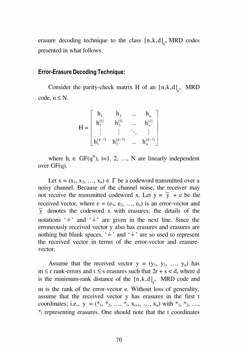
8/2/2019 Erasure Techniques in MRD Codes, by W. B. Vasantha Kandasamy, Florentin Smarandache, R. Sujatha, R. S. Raja …
http://slidepdf.com/reader/full/erasure-techniques-in-mrd-codes-by-w-b-vasantha-kandasamy-florentin-smarandache 71/164
70
erasure decoding technique to the class Nq
[n,k,d] MRD codes
presented in what follows.
Error-Erasure Decoding Technique:
Consider the parity-check matrix H of an Nq[n,k,d] MRD
code, n ≤ N.
H =
1 2 n
[1] [1] [1]1 2 n
[d 2] [d 2] [d 2]
1 2 n
h h ... h
h h ... h
h h ... h− − −
where hi ∈ GF(qN), i=1, 2, …, N are linearly independent
over GF(q).
Let x = (x1, x
2, …, x
n) ∈ Γ be a codeword transmitted over a
noisy channel. Because of the channel noise, the receiver may
not receive the transmitted codeword x. Let y = y + e be the
received vector, where e = (e1, e2, …, en) is an error-vector and
y denotes the codeword x with erasures; the details of the
notations ‘ ’ and ‘ + ’ are given in the next line. Since the
erroneously received vector y also has erasures and erasures are
nothing but blank spaces, ‘ ’ and ‘ + ’ are so used to represent
the received vector in terms of the error-vector and erasure-
vector.
Assume that the received vector y = (y1, y2, …, yn) has
m ≤ r rank-errors and t ≤ s erasures such that 2r + s < d, where d
is the minimum-rank distance of the Nq[n,k,d] MRD code and
m is the rank of the error-vector e. Without loss of generality,
assume that the received vector y has erasures in the first t
coordinates; i.e., y = (*1, *2, …, *t, xt+1, …, xn) with *1, *2, …,*t representing erasures. One should note that the t coordinates

8/2/2019 Erasure Techniques in MRD Codes, by W. B. Vasantha Kandasamy, Florentin Smarandache, R. Sujatha, R. S. Raja …
http://slidepdf.com/reader/full/erasure-techniques-in-mrd-codes-by-w-b-vasantha-kandasamy-florentin-smarandache 72/164
71
of e that are corresponding to the erasures in the received vector
y are zeros; i.e., e1, e2, …, et are all zero. Therefore, e =
(0,0,...,0
t terms
, et+1, et+2, …, en). Then the received vector takes the
form y (*1, *2, …, *t, xt+1, …, xn) + (0, 0, …, 0, et+1, et+2, …,en).
Let f = (f 1, f 2, …, f t, (0,0,...,0
n t terms−
) be the erasure-vector.
Let 1 2 ny (y , y ,..., y )′ ′ ′ ′= be such that i ii
i
f if x iserasedyx otherwise′ =
,
where the unknowns f 1, f 2, …, f t (t ≤ s) are to be determined.
Then y′ = (f 1, f 2, …, f t, xt+1, …, xn). Having replaced the
erasures with the unknown f 1, f 2, …, f t, the received vector y is
now expressed as y′ + e; i.e., y = y′+ e. The syndrome of y is
given by
S = y HT
= ( y′ + e)HT
= (f 1, f 2, …, f t, xt+1, …, xn)HT
+ (0, 0, …, 0, et+1, …, en)HT
= (f 1, f 2, …, f t, xt+1, et+1, …, xn + en) HT
. (4.2)
The decoder’s problem is to first determine the error-vector
e = (0, 0, …, 0, et+1, …, en) and then the erasure-vectorf = (f 1, f 2, …, f t, 0, …, 0) on the basis of the syndrome vector
S = (s0, s1, …, sd-2), where si denotes the ith
coordinates of S for
each i = 0, 1, … d–2.
Equating each component in the right-hand side of (4.2),
f 1 h1 + … + f t ht + (xt+1 + et+1) ht+1 + … + (xn + en) hn = 0

8/2/2019 Erasure Techniques in MRD Codes, by W. B. Vasantha Kandasamy, Florentin Smarandache, R. Sujatha, R. S. Raja …
http://slidepdf.com/reader/full/erasure-techniques-in-mrd-codes-by-w-b-vasantha-kandasamy-florentin-smarandache 73/164
72
f 1 [1]
1h + … + f t [1]
th + (xt+1 + et+1)[1]
t 1h +
+ … + (xn + en)[1]
nh = 0
f 1
[d 2]
1h − + … + f t [d 2]
th − + (xt+1 + et+1)[d 2]
t 1h −+
+ … + (xn + en)[d 2]
nh − = 0
Let ( )(0 )
jθ denote the equation
f 1 [ j]
1h + … + f t [ j]
th + (xt+1 + et+1)[ j]
t 1h + + … + (xn + en)[ j]
nh = 0
for each j = 0, 1, …, d–2 and θ(d-1)= ( )( (0)
0θ , ( )(0)
1θ , …, ( ))(0)
d 2−θ
represent the above system of d–1 equations ( )(0 )
0θ , ( )(0 )
1θ , …,
( )(0)
d 2−θ .
In the above system θ(d–1)of d–1 equations, one needs to
eliminate f 1, f 2, …, f t. For each i = 1, 2,…, t, the elimination of
f i, results in a system, say θ(d–1–i), of d–1–i equations, say ( )(i)
0θ ,
( )(i )
1θ , …, ( )(i )
d 2 i− −θ . Let θ(d–1–i)= ( ( )(i )
0θ , ( )(i )
1θ , …, ( )(i )
d 2 i− −θ ).
Therefore, θ(d–1–t)= ( )( ( t)
0θ , ( )(t )
1θ , …, ( ))(t )
d 2 t− −θ would
represent the system θ(d–1–t)of d–1–t equations obtained after the
elimination f 1, f 2, …, f t from the system θ(d–1).
The recursive procedure for the elimination of f 1, f 2, …, f t
from the system θ(d–1)= ( )(0)
0θ , ( )(0)
1θ , …, ( )(0)
d 2−θ is given as
follows.
For each i = 1, 2, …, t, perform the operation.
Define
Z(i–1)=
(i 1) (d i)
i(i 1) (d i)
i 0
Coefficient of f in equation (θ
) of systemθ
Coefficient of f in equation (θ ) of system θ
− −
− − .

8/2/2019 Erasure Techniques in MRD Codes, by W. B. Vasantha Kandasamy, Florentin Smarandache, R. Sujatha, R. S. Raja …
http://slidepdf.com/reader/full/erasure-techniques-in-mrd-codes-by-w-b-vasantha-kandasamy-florentin-smarandache 74/164
73
Then (to eliminate f i from the system θ(d–i)of d–i equations)
multiply the equation ( )(i 1)
j
−θ by[ j]
(i 1)Z − and subtract the equation
( )(i 1)
j 1
−+θ from the equation ( )(i 1)
j
−θ for each j = 0, 1, 2, …, d–2–i.
Then one obtains the system θ(d–1–i)= ( )( (i )
0θ , ( )(i)
1θ , …,
( ))(i )
d 2 i− −θ of d–1–i equations after the elimination of f i.
The reduced system θ(d–1–t)of d–1–t equations ( )(t )
0θ ,
( )(t )1θ , …, ( )
(t)d 2 t− −θ after the elimination of f 1, f 2, …, f t from the
system θ(d–1)= ( )( (0)
0θ , ( )(0 )
1θ , …, ( ))(0)
d 2−θ is of the following
form.
0s′ = (xt+1 + et+1) t 1h +′ + (xt+2 + et+2) t 2h +
′ + … + (xn + en) nh′
1s′ = (xt+1 + et+1)[1]
t 1h +′ + (xt+2 + et+2)
[1]
t 2h +′ + … + (xn + en)
[1]
nh′
and d 2 ts − −
′ = (xt+1 + et+1)[d 2 t]
t 1h − −+
′ + (xt+2 + et+2)[d 2 t]
t 2h − −+
′
+ … + (xn + en)[d 2 t]
nh − −′ .
The above system of equations can be rewritten as,
( 0s′ , …, d 2 ts − −′ )
= (xt+1 + et+1, …, xn + en)
T
1 2 n[1] [1] [1]
t 1 t 2 n
[d 2 t] [d 2 t] [d 2 t ]
t 1 t 2 n
h h ... hh h ... h
h h ... h
+ +
− − − − − −
+ +
′ ′ ′ ′ ′ ′
′ ′ ′
= (xt+1 + et+1 , …, xn + en)T(t)
H
= (xt+1, …, xn)
T(t)
H + (et+1, …, en)
T(t)
H

8/2/2019 Erasure Techniques in MRD Codes, by W. B. Vasantha Kandasamy, Florentin Smarandache, R. Sujatha, R. S. Raja …
http://slidepdf.com/reader/full/erasure-techniques-in-mrd-codes-by-w-b-vasantha-kandasamy-florentin-smarandache 75/164
74
= x(t)
T(t)
H + e(t)
T(t )
H
= (0) + e
(t)
T(t)
H (by Lemma 4.2.2)
= e(t)
T(t)
H
i.e., ( 0s′ , …, d 2 ts − −′ ) = e
(t)
T(t )H (4.3)
wheree
(t)= (et+1, et+2, …, en) is the deletion of the first
t coordinates of e and
H(t)
=
t 1 t 2 n
[1] [1] [1]
t 1 t 2 n
[d 2 t] [d 2 t] [d 2 t]
t 1 t 2 n
h h ... h
h h ... h
h h ... h
+ +
+ +
− − − − − −
+ +
′ ′ ′ ′ ′ ′
′ ′ ′
is the (d–1–t) × (n–t) matrix, which is the deletion of the firstt columns of H.
If is′ = 0 for each i, then it is concluded that the received
vector y contains no errors. Then solving the system θ(d–1)of
d–1 equations, one can determine the values for the unknowns
f 1, f 2, …, f t. If is′ ≠ 0 for some i, then the received vector y
contains errors. To find the error-vector
e = (0, 0, …, 0, et+1, et+2, …, en), one is to continue the
following procedure with the known syndrome values is′ ,
i = 0, 1, …, d–2–t. Actually, one needs to find the error vector
e(t)
= (et+1, et+2, …, en).
Since the rank norm of the error-vector e is assumed to be
m, e(t)
can be written in the following form:
e(t)
= EY = (E1, E2, …, Em)Y, (4.4)

8/2/2019 Erasure Techniques in MRD Codes, by W. B. Vasantha Kandasamy, Florentin Smarandache, R. Sujatha, R. S. Raja …
http://slidepdf.com/reader/full/erasure-techniques-in-mrd-codes-by-w-b-vasantha-kandasamy-florentin-smarandache 76/164
75
where (E1, E2, …, Em) are linearly independent over GF(q), and
Y =m,n
ij i , j 1,t 1Y
= + is an m × (n – t) matrix of rank m with entries
from GF(q).
Equation (4.3) becomes,
( 0s′ , …, d 2 ts − −′ ) = EY
T(t)H = EX, (4.5)
where the transposed matrix of X = YT(t)H has the form
XT =
1 2 m
[1] [1] [1]
1 2 m
[d 2 t ] [d 2 t ] [d 2 t]
1 2 m
x x ... x
x x ... x
x x ... x− − − − − −
′ ′ ′
′ ′ ′
′ ′ ′
(4.6)
andn
p pj j
j t 1
x Y h= +
′ ′= ∑ , p = 1, 2, …, m. (4.7)
are linearly independent over GF(q).
Equation (4.5) is equivalent to the following system of
equations in the unknowns E1, E2, …, Em, 1 2 mx , x ,..., x′ ′ ′ ,
m[p ]
p i i
i 1
s E x=
′ ′= ∑ , p = 0, 1, …, d–2–t. (4.8)
If the solution of the system (4.8) has been found, then from
(4.7) and (4.4), one can determine the matrix Y and the error-vector e
(t)respectively. Note that the above system (4.8) has
many solutions for a specified m; for m ≤d 1 t
2
− −
. However,
all solutions lead to the same vector e(t)
. Thus, the decoding
problem reduces to finding the solution of the system (4.8).
Let S′(z) =d 2 t [ j]
j j 0s z
− −
=′∑ be termed as the syndrome
polynomial.

8/2/2019 Erasure Techniques in MRD Codes, by W. B. Vasantha Kandasamy, Florentin Smarandache, R. Sujatha, R. S. Raja …
http://slidepdf.com/reader/full/erasure-techniques-in-mrd-codes-by-w-b-vasantha-kandasamy-florentin-smarandache 77/164
76
Set F0(z) = z[d–1–t]
, F1(z)=S′(z) and employ Euclid’s divisionalgorithm until reaching a remainder polynomial Fm+1(z) such
that deg(Fm(z)) ≥ q(d–1–t)/2
and deg(Fm+1(z)) < q(d–1–t)/2
. Then it is
concluded that the received vector y has m rank-errors; that is,r[e
(t); q] = m.
Let ∆(z) =m [p]
pp 0z
=∆∑ , ∆m = 1 be a polynomial whose roots
are all possible linear combinations of E1, E2, …, Em withcoefficients from GF(q).
Using the coefficients of the remainder polynomial Fm+1(z),
the coefficients ∆0, ∆1, …, ∆m of the polynomial ∆(z) can bedetermined recursively as follows:
Let j be such that is′= 0 and js′ ≠ 0 for i < j.
Then ∆0 = f j / js′ ,
∆p = (f j+p –p i
[i] [p]i p j 1 ji 0 / s ,−
− + −= ′∆∑ p = 1, 2, …, m,
where f j is the coefficient of Fm+1(z) for degree [j] and for
j + p ≥ m, set f j+p = 0.
Determine the roots E1, E2, …, Em of ∆(z) that are linearlyindependent over GF(q). Methods for determining the roots of
∆(z) are described in [25]. After determining the roots E1, E2,
…, Em of ∆(z), consider the following truncated system;
m[p ]
p i i
i 1
s E x=
′ ′= ∑ , p = 0, 1, …, m–1 (4.9)
Solving the system (4.9), one obtains [p]
jx′ and hence the
error-vector e(t)
. Then, by substituting e(t)
in the system θ(d–1)of d
– 1 equations, one can determine the values for the unknowns f 1,f 2, …, f t. Hence x = y – e, which is the actually transmittedcodeword.

8/2/2019 Erasure Techniques in MRD Codes, by W. B. Vasantha Kandasamy, Florentin Smarandache, R. Sujatha, R. S. Raja …
http://slidepdf.com/reader/full/erasure-techniques-in-mrd-codes-by-w-b-vasantha-kandasamy-florentin-smarandache 78/164
77
Summary of the error-erasure decoding technique:
Step 1: Compute the syndrome values ( 0s′ , …, d 2 ts − −′ ) for
the vector y = (f 1, f 2, …, f t, xt+1, …, xn) + (0, 0, …, 0, et+1, …, en)and the corresponding syndrome polynomial
S′(z) =d 2 t [ j]
j j 0s z
− −
=′∑ .
Step 2: Set F0(z) = z[d–1–t]
, F1(z) = S′(z) and employ Euclid’sdivision algorithm until reaching a Fm+1(z) such that deg (Fm(z))
> q(d–1–t)/2
and deg (Fm+1(z)) < q(d–1–t)/2
. Let ∆(z) =
m [p ]
pp 0 z= ∆∑ ,
∆m = 1 be such that its roots are all possible linear combinationsof E1, E2, …, Em over GF(q).
Step 3: Determine the coefficients of ∆(z) as follows:
Let j be such that is′ = 0 and js′ ≠ 0 for i < j.
∆0 = f j / j
s′ ,
∆p = (f j+p,p i [i] [p]
i p j 1 ji 0 / s ,
−
− + −=′∆∑ p = 1, 2, …, m.
where f j is the coefficient of Fm+1(z) for degree [j] and
f j+p = 0 for j + p ≥ m.
Step 4: Compute the roots E1, E2, …, Em of ∆(z) that are
linearly independent over GF(q). Then, by substituting E1, E2,…, Em in system (4.9), one can determine
[p]
jx and hence the
error-vector e(t)
.
Step 5: Substituting e(t)
in system θ(d–1), one can obtain the
values for the unknown f 1, f 2, …, f t.
Step 6: The transmitted codeword is then obtained as
x = y – e.

8/2/2019 Erasure Techniques in MRD Codes, by W. B. Vasantha Kandasamy, Florentin Smarandache, R. Sujatha, R. S. Raja …
http://slidepdf.com/reader/full/erasure-techniques-in-mrd-codes-by-w-b-vasantha-kandasamy-florentin-smarandache 79/164
78
Using the combined error-erasure decoding technique to the
class of Nq[n,k,d] MRD codes presented above, one can correct
any combination of m ≤ r rank-errors and t ≤ s erasures in anerroneously received vector as long as 2r + s < d, where d is theminimum-rank distance of the MRD codes.
A detailed description of the combined error-erasure
decoding technique to the class of N2[n,k,d] MRD codes
presented above is demonstrated through the following examplewhich applies the combined error-erasure decoding technique to
the 82[7,1,7] MRD code for the correction of 2 errors and 2
erasures in an erroneously received vector.
Example 4.2.1: Let Γ = 82[7,1,7] be the MRD code defined
over GF(28) = {0, 1, α, …,
82 2−α } with the parity-check matrix
H:
H =
2 3 4 5 6
2 4 6 8 10 12
4 8 12 16 20 24
8 16 24 32 40 48
16 32 48 64 80 96
32 64 96 128 160 192
1
1
1
1
1
1
α α α α α α
α α α α α α α α α α α α
α α α α α α α α α α α α
α α α α α α
where α is a root of the primitive polynomialx8
+ x6
+ x5
+ x + 1 over GF(2).
Let x = (0, 0, 0, 0, 0, 0, 0) ∈ Γ be the transmitted codeword
and y = α31, α147
, 0, 0, *5, 0, *7) be the received vector, where‘*5’ and ‘*7’ represent erasures. Note that the received vector yhas two erasures.
Let f = (0, 0, 0, 0, f 5, 0, f 7). Then replacing the erasures with
unknowns f 5 and f 7, one has the vector y′ = (α31, α147, 0, 0, f 5, 0,f 7) where the unknowns f 5 and f 7 are to be determined. Let e =

8/2/2019 Erasure Techniques in MRD Codes, by W. B. Vasantha Kandasamy, Florentin Smarandache, R. Sujatha, R. S. Raja …
http://slidepdf.com/reader/full/erasure-techniques-in-mrd-codes-by-w-b-vasantha-kandasamy-florentin-smarandache 80/164
79
(e1, e2, e3, e4, 0, e6, 0) be the error-vector to be determined. Then
x = y′ – e would be the transmitted code word. The syndrome of
y′ – e is
S = (y′ – e)HT
= (α31, α147
, 0, 0, f 5, 0, f 7)HT
– (e1, e2, e3, e4, 0, e6, 0)HT
(4.10)
Equating each component on the right-hand side of (4.10) to
0,
α4f 5 + α6
f 7 + 1 = e1 + αe2 + α2e3 + α3
e4 + α5e6,
α8f 5 + α12
f 7 + α147= e1 + α2
e2 + α4e3 + α6
e4 + α10e6,
α16f 5 + α24
f 7 + α108= e1 + α4
e2 + α8e3 + α12
e4 + α20e6,
α32f 5 + α48
f 7 + α113= e1 + α8
e2 + α16e3 + α24
e4 + α40e6,
α64f 5 + α96
f 7 + α41= e1 + α16
e2 + α32e3 + α48
e4 + α80e6,
and
α128f 5 + α192
f 7 + α62= e1 + α32
e2 + α64e3 + α96
e4 + α160e6.
Let θ(6)= ( )( (0 )
0θ , ( )(0)
1θ , ( )(0)
2θ , ( )(0 )
3θ , ( )(0 )
4θ , ( ))(0)
5θ
denote the above system of 6 equations.
Here
Z(0) =(0) (6)
5 1
(0) (6)
5 0
Coefficient of f in equation (θ ) of system θ
Coefficient of f in equation (θ ) of system θ= α4
.
The eliminate f 5 from the above system θ(6)of 6 equations,
multiply the equation ( )(0 )
jθ by[ j]
(0)Z and subtract the equation
( )(0)
j 1+θ from the equation ( )(0 )
jθ for each j = 0, 1, 2, 3, 4. Then
one obtains the following reduced system θ(5)= ( )( (1)
0θ , ( )(1)
1θ ,
( )(1)
2θ , ( )(1)
3θ , ( ))(1)
4θ of 5 equations after the elimination of f 5.

8/2/2019 Erasure Techniques in MRD Codes, by W. B. Vasantha Kandasamy, Florentin Smarandache, R. Sujatha, R. S. Raja …
http://slidepdf.com/reader/full/erasure-techniques-in-mrd-codes-by-w-b-vasantha-kandasamy-florentin-smarandache 81/164
80
α149f 7 + α78
= α23e1 + α52
e2 + α143e3 + α203
e4 + α206e6,
α43f 7 + α105
= α46e1 + α104
e2 + α31e3 + α151
e4 + α157e6,
α86f 7 + α104
= α92e1 + α208
e2 + α62e3 + α47
e4 + α59e6,
α172 f 7 + α16 = α184e1 + α161 e2 + α124 e3 + α94 e4 + α118 e6,
and
α89f 7 + α240
= α113e1 + α67
e2 + α248e3 + α188
e4 + α236e6.
Now
Z(1) =(1) (5)
7 1
(1) (5)
7 0
Coefficient of f in equation (θ ) of system θ
Coefficient of f in equation (θ ) of system θ=α149
.
To eliminate f 7 from the above system θ(5)of 5 equations,
multiply the equation ( )(1)
jθ by[ j]
(1)Z and subtract the equation
( )(1)
j 1+θ from the equation ( )(1)
jθ for each j = 0, 1, 2, 3. Then one
obtains the following reduced system θ
(4)
= ( )((1)
0θ , ( )
(1)
1θ ,
( )(1)
2θ , ( ))(1)
3θ of 4 equations after the elimination of f 7.
α95= α197
e1 + α71e2 + α131
e3 + α196e4 + α10
e6,
α68= α139
e1 + α142e2 + α7
e3 + α137e4 + α20
e6,
α44= α23
e1 + α29e2 + α14
e3 + α19e4 + α40
e6,
and α48= α46
e1 + α58e2 + α28
e3 + α38e4 + α80
e6.
The above system θ(4)of 4 equations can be written as
(α95, α68
, α44, α48
)
= (e1, e2, e3, e4, e6)
T197 71 131 196 10
139 142 7 137 20
23 29 14 19 40
46 58 28 38 80
α α α α α α α α α α
α α α α α
α α α α α
(4.11)

8/2/2019 Erasure Techniques in MRD Codes, by W. B. Vasantha Kandasamy, Florentin Smarandache, R. Sujatha, R. S. Raja …
http://slidepdf.com/reader/full/erasure-techniques-in-mrd-codes-by-w-b-vasantha-kandasamy-florentin-smarandache 82/164
81
Let ( )0 1 2 3s ,s ,s ,s′ ′ ′ ′ = (α95, α68
, α44, α48
)
and e(2)
= (e1, e2, e3, e4, e6)
Here S′(z) = α95z
[0]+ α68
z[1]
+ α44z
[2]+ α48
z[3]
.
Let F0(z) = z[4]
and
F1(z) = α95z + α68
z2
+ α44z
4+ α48
z8
Dividing F0(z) on the right by F1(z).
F0(z) = (α207z
8+ α203
z4
+ α227z
2+ α254
z + α199)
* F1(z) + F2(z).
where F2(z) = α103z
4+ α136
z2
+α39z.
Dividing F1(z) on the right by F2(z).
F1(z) = (α200z
4+ α233
z2
+ α136z) * F2(z) + F3(z),
where F3(z) = α48
z2
+ α72
z.
Since deg(F2 (z)) = 4 ≥ 22
and deg (F3 (z)) = 2 < 22, it follows
the received vector has m = 2 rank-errors i.e., r [e(2)
; 2] = 2.
Since e(2)
is of rank norm m = 2,
e(2)
= (E1, E2)11 12 13 14 16
21 22 23 24 26
Y Y Y Y Y
Y Y Y Y Y
(4.12)
= ( )1 2 3 4 6Y , Y ,Y ,Y ,Y (say)
where E1 and E2 are linearly independent over GF(2), and
Y = [Yij] is the 2 × 5 matrix of rank 2 with entries from GF(2).
Equation (4.11) becomes,
(α95, α68, α44, α48)

8/2/2019 Erasure Techniques in MRD Codes, by W. B. Vasantha Kandasamy, Florentin Smarandache, R. Sujatha, R. S. Raja …
http://slidepdf.com/reader/full/erasure-techniques-in-mrd-codes-by-w-b-vasantha-kandasamy-florentin-smarandache 83/164
82
= ( )1 2 3 4 6Y , Y ,Y ,Y ,Y
T197 71 131 196 10
139 142 7 137 20
23 29 14 19 40
46 58 28 38 80
α α α α α α α α α α
α α α α α α α α α α
(4.13)
Here ∆ (z) =∆0 Z[0]
+ ∆1 Z[1]
+ ∆2 Z[2]
with ∆0 = α232,
∆1 = α160and ∆2 = α160
.
The roots of ∆ (z) are α31, α147
, α149and 0. Take E1 = α31
,
and E2 = α147.
α95=
197 71 131 196 10
1 11 12 13 14 16
197 71 131 196 10
2 21 22 23 24 26
E ( y y y y y )
E ( y y y y y )
α + α + α + α + α +
α + α + α + α + α
and
α68=
139 142 7 137 20
1 11 12 13 14 16
139 142 7 137 20
2 21 22 23 24 26
E ( y y y y y )
E ( y y y y y )
α + α + α + α + α +
α + α + α + α + α
.
Solving the above equation,
Y =1 0 0 0 0
0 1 0 0 0
.
Therefore, e = (α31, α147
, 0, 0, 0, 0, 0). By substituting
e = (α31, α147, 0, 0, 0, 0, 0) in the system θ(6) of 6 equations, oneobtains f 5 = 0 and f 7 = 0.
Hence x = y′ – e
= (α31, α147
, 0, 0 , 0, 0, 0) – (α31, α147
, 0, 0, 0, 0, 0)
= (0, 0, 0, 0, 0, 0, 0),
which is the actually transmitted codeword.

8/2/2019 Erasure Techniques in MRD Codes, by W. B. Vasantha Kandasamy, Florentin Smarandache, R. Sujatha, R. S. Raja …
http://slidepdf.com/reader/full/erasure-techniques-in-mrd-codes-by-w-b-vasantha-kandasamy-florentin-smarandache 84/164
83
4.3 Invertible q-Cyclic RD Codes
There are two categories of techniques for controllingtransmission errors in data transmission systems: the Forward-Error Control (FEC) scheme and the Automatic-Repeat –
Request (ARQ) scheme. In an FEC system, an error-correcting
code is used, when the receiver detects the presence of errors in
a received vector, it attempts to determine the error locationsand then corrects the errors. If the exact locations of errors are
determined, the received vector will be correctly decoded; if the
receiver fails to determine the exact locations of errors, thereceived vector will be decoded incorrectly and erroneous data
will be delivered to be destination. In an ARQ system, a code
with good error-detecting capability is used. At the receiver, thesyndrome of the received vector is computed. If the syndrome is
zero, the received vector is assumed to be error-free and is
accepted by the receiver. At the same time, the receiver notifies
the transmitter, via a return channel, that the transmittedcodeword has been successfully received. If the syndrome is not
zero, errors are detected in the received vector. Then thetransmitter is instructed, through the return channel, toretransmit the same codeword. Retransmission continues until
the codeword is successful received.
The throughput efficiency (or throughput) is a measure of
performance of an ARQ system. Throughout efficiency is
defined as the ratio of the average number of information
symbols successfully accepted by the receiver per unit of timeto the total number of symbols that could be transmitted per unit
of time. The retransmission of an erroneously received vector
continues until the received vector is successfully received bythe receiver. Though the retransmission requests provide a
powerful means of improving reliability performance at the cost
of a reduction in throughput, the frequency of retransmission
must be reduced to improve the throughout efficiency. Bothsystems have their own limitations and drawbacks. To improve
the throughput efficiency, a hybrid - ARQ scheme which is acombination of both FEC and ARQ, came into existence [25].
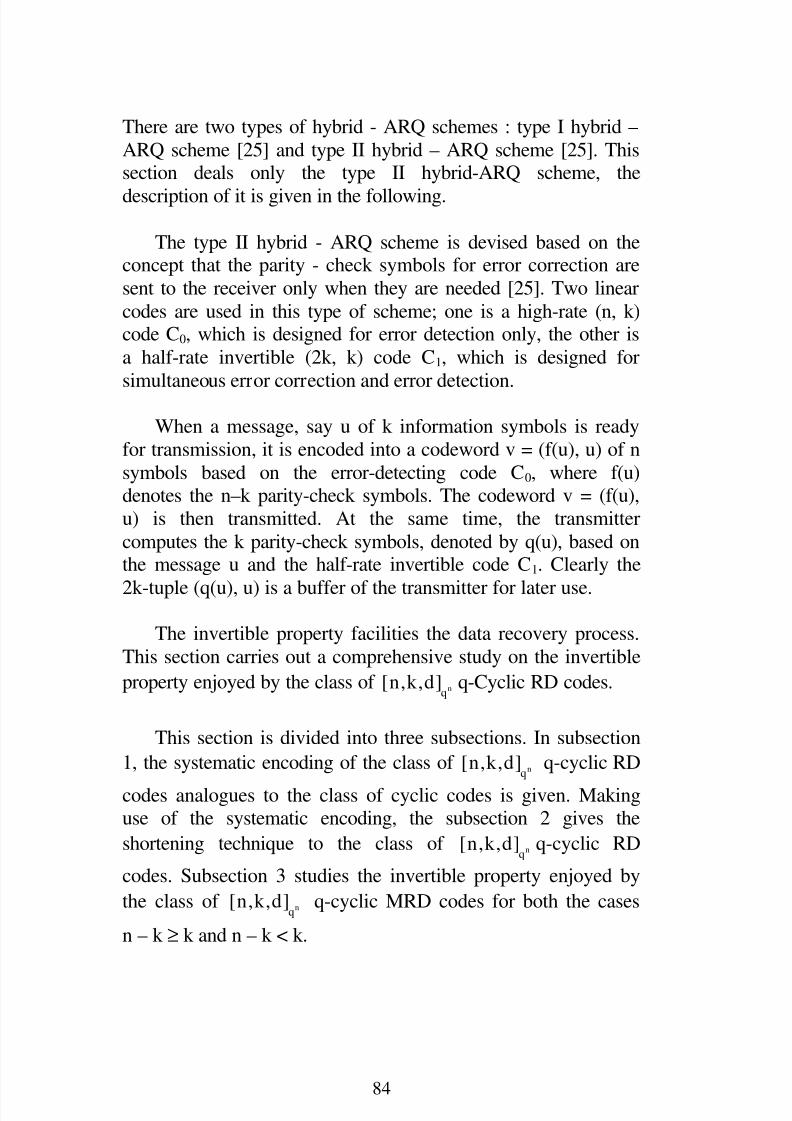
8/2/2019 Erasure Techniques in MRD Codes, by W. B. Vasantha Kandasamy, Florentin Smarandache, R. Sujatha, R. S. Raja …
http://slidepdf.com/reader/full/erasure-techniques-in-mrd-codes-by-w-b-vasantha-kandasamy-florentin-smarandache 85/164
84
There are two types of hybrid - ARQ schemes : type I hybrid –
ARQ scheme [25] and type II hybrid – ARQ scheme [25]. Thissection deals only the type II hybrid-ARQ scheme, the
description of it is given in the following.
The type II hybrid - ARQ scheme is devised based on theconcept that the parity - check symbols for error correction are
sent to the receiver only when they are needed [25]. Two linear
codes are used in this type of scheme; one is a high-rate (n, k)code C0, which is designed for error detection only, the other is
a half-rate invertible (2k, k) code C1, which is designed for
simultaneous error correction and error detection.
When a message, say u of k information symbols is ready
for transmission, it is encoded into a codeword v = (f(u), u) of n
symbols based on the error-detecting code C0, where f(u)denotes the n–k parity-check symbols. The codeword v = (f(u),
u) is then transmitted. At the same time, the transmitter
computes the k parity-check symbols, denoted by q(u), based onthe message u and the half-rate invertible code C1. Clearly the
2k-tuple (q(u), u) is a buffer of the transmitter for later use.
The invertible property facilities the data recovery process.
This section carries out a comprehensive study on the invertible
property enjoyed by the class of nq[n,k,d] q-Cyclic RD codes.
This section is divided into three subsections. In subsection
1, the systematic encoding of the class of nq[n,k,d] q-cyclic RD
codes analogues to the class of cyclic codes is given. Makinguse of the systematic encoding, the subsection 2 gives the
shortening technique to the class of nq
[n,k,d] q-cyclic RD
codes. Subsection 3 studies the invertible property enjoyed by
the class of nq
[n,k,d] q-cyclic MRD codes for both the cases
n – k ≥ k and n – k < k.

8/2/2019 Erasure Techniques in MRD Codes, by W. B. Vasantha Kandasamy, Florentin Smarandache, R. Sujatha, R. S. Raja …
http://slidepdf.com/reader/full/erasure-techniques-in-mrd-codes-by-w-b-vasantha-kandasamy-florentin-smarandache 86/164
85
Systematic Encoding of q-Cyclic RD Codes
The generator and parity-check matrices for linear codes
greatly simplify encoding at the transmitter and error detectionat the receiver. The problem of recovering the message block
from a codeword can be greatly simplified through the use of systematic encoding. As in the case of ordinary cyclic codes,
systematic encoding for the class of nq[n,k,d] q-Cyclic RD
codes can be done either by means of a generator polynomial or
by means of a generator matrix in systematic (or standard) form.
(a) Systematic encoding through generator polynomial
Let G(z) =n k [i ]
ii 0G z
−
=∑ be the given generator polynomial
of an nq
[n,k,d] q-Cyclic RD code, say C.
Let H(z) =k [i ]
ii 0H z
=∑ be such that z[n]
– z = H(z) * G(z). If
one assumes that gn–1, gn–2, …, gn–k are information symbols,
then s/he can determine the parity-check symbols gn–k–1, gn–k–2,…, g0 as follows.
Let u(z) = gn–1z[n–1]
+ gn–2z[n–2]
+ … + gn–k z[n–k]
be a message
polynomial to be encoded.
Divide u(z) on the right by G(z);
u(z) = q(z) * G (z) + f(z), deg (f (z)) < [n–k].
where q(z) is the quotient polynomial and f(z) is the remainder
polynomial.
Then the coefficients gn–i for degree gn–i for degree [n–i],
i = k+1, k+2, …, n of the remainder polynomial f (z) will be the
parity-check symbols. Then g(z) = u(z) – f(z) is thesystematically encoded code polynomial corresponding to the
message polynomial u(z), where f(z) is called as the parity-check polynomial.

8/2/2019 Erasure Techniques in MRD Codes, by W. B. Vasantha Kandasamy, Florentin Smarandache, R. Sujatha, R. S. Raja …
http://slidepdf.com/reader/full/erasure-techniques-in-mrd-codes-by-w-b-vasantha-kandasamy-florentin-smarandache 87/164
86
(b) Systematic encoding through generator matrix
The systematic encoding of the nq[n,k,d] q-cyclic RD code
C can also be carried out through generator and parity-check
matrices in systematic form. This is accomplished in thefollowing.
The generator matrix and the parity-check matrix
corresponding to G(z) and H(z) of C in systematic form can be
obtained as follows:
Dividing z[n–k+i]
on the right by G(z) for each i = 0, 1, …,k–1, one gets
z[n–k+i]
= qi(z) * G(Z) + f i(z), where qi(z) is the quotientpolynomial and f i(z) = f i0z
[0]+ f i1z
[1]+ … + f i, n–k–1z
[n–k–1]is the
remainder polynomial.
Since G(z) is a right divisor of z[n–k–i] – f i(z), i = 0, 1, …,k–1, they are code polynomials of C.
Arranging these k code polynomials as rows of a k × nmatrix, one obtains the matrix say G:
G =
00 01 0,n k 1
01 11 1,n k 1
k 1,0 k 1,1 k 1,n k 1
f f ... f 1 0 0 ... 0
f f ... f 0 1 0 ... 0
0
f f ... f 0 0 0 ... 1
− −
− −
− − − − −
which is the generator matrix of C in systematic form. Recall
that any set of k linearly independent vectors can be used as the
rows of the generator matrix to form a k-dimensional linear
code.

8/2/2019 Erasure Techniques in MRD Codes, by W. B. Vasantha Kandasamy, Florentin Smarandache, R. Sujatha, R. S. Raja …
http://slidepdf.com/reader/full/erasure-techniques-in-mrd-codes-by-w-b-vasantha-kandasamy-florentin-smarandache 88/164
87
The corresponding parity-check matrix, say H in systematicform is given by
H =
00 10 k 1,0
01 11 k 1,1
0,n k 1 1,n k 1 k 1,n k 1
1 0 0 ... 0 f f ... f
0 1 0 ... 0 f f f
0 0 0 ... 1 f f ... f
−
−
− − − − − − −
− − − − − −
− − −
Note that GHT
= (0). If u = (gn–k , gn–k+1, …, gn–1) is a
message vector, then v = uG = (g0, g1, …, gn–1) is thesystematically encoded codeword corresponding to the message
vector u and one can note that HT
= (0), where g0, g1, …, gn–k–1
are the corresponding parity-check symbols.
The systematic encoding for the class of nq[n,k,d] q-Cyclic
RD codes given above is demonstrated through the following
example.
Example 4.3.1.1: Consider the [ ] 525,3 2-Cyclic RD code
generated by G(z) = α24z + α3
z2
+ α2z
4, where α is a root of
the primitive polynomial x5
+ x2
+ 1 over GF(2).
Dividing z[2]
on the right by G[z], one gets
z4
= α29z * G (z) + αz
2+ α22
z with f 1(z) = α z2
+ α22z.
Dividing z[3]
on the right by G[z], one gets
z8
= (α27z
2+ z) * G (z) + α7
z2
+ α24z with
f 2 (z) = α7z
2+ α24
z.
Dividing z[4]
on the right by G[z], one gets
Z
16
= (α
23
z
4
+ z
2
+ α
12
z) * G(z) + α
20
z
2
+ α
5
z withf 3(z) = α20
z2
+ α5z.

8/2/2019 Erasure Techniques in MRD Codes, by W. B. Vasantha Kandasamy, Florentin Smarandache, R. Sujatha, R. S. Raja …
http://slidepdf.com/reader/full/erasure-techniques-in-mrd-codes-by-w-b-vasantha-kandasamy-florentin-smarandache 89/164
88
Then the generator matrix G and the parity-check matrix H
for the 52
[5,3] 5-Cyclic RD code in systematic form are
respectively given by
G =
22
24 7
5 20
1 0 0
0 1 0
0 0 1
α α α α
α α
and
H =
22 24 5
7 20
1 0
0 1
α α α
α α α .
Let u1(z) = α5z
[4]+ z
[3]+ α23
z[2]
be the message polynomialto be encoded. Dividing u1(z) on the right by G(z), one gets.
u1(z) = (α28z
4+ α12
z2
+ α6z) * G(z) + α17
z2
+ α30z.
Then g1(z) = α
30
z + α
17
z
[1]
+ α
23
z
[2]
+ z
[3]
+ α
5
z
[4]
is thesystematically encoded code polynomial corresponding to themessage polynomial u1(z). Note also that
(α30, α17
, α23, 1, α5
) HT
= (0).
Similarly, g2(z) = α13z + α11
z[1]
+ α9z
[2]+ 0z
[4]is the code
polynomial corresponding to the message polynomial u2(z) =
0z[4]
+ α21z
[3]+ α9
z[2]
and that (α13, α11
, α9, α21
, 0) HT
= (0).
The next subsection gives the shortening technique to the
class of nq
[n,k,d] q-Cyclic RD codes. In shortening of an
nq
[n,k, d] q-Cyclic RD code, each codeword is shortened (in
length) by t information symbols, resulting in a linear code of
length n – t, dimension k – t with the same error-correcting
capability as the original code, t < k.

8/2/2019 Erasure Techniques in MRD Codes, by W. B. Vasantha Kandasamy, Florentin Smarandache, R. Sujatha, R. S. Raja …
http://slidepdf.com/reader/full/erasure-techniques-in-mrd-codes-by-w-b-vasantha-kandasamy-florentin-smarandache 90/164
89
4.3.2 Shortened q-Cyclic RD codes
In many applications, there are external constraints such as
puncturing, extending, shortening, lengthening, expurgating, oraugmenting [25], which are unrelated to error-control but
determine the allowed length of the error-control code. Insystem design, if a code of suitable length or suitable number of
information symbols can not be found, it may be possible to
shorten a code to meet the requirements. In extending, a code isextended by adding an additional redundant coordinate. Thus an
(n, k) code becomes an (n + 1, k) code. In shortening, a code is
shortened by deleting a message coordinate from the encodingprocess. Thus an (n, k) code becomes an (n – 1, k – 1) code.
This section gives shortening technique to the class of nq[n,k,d]
q-Cyclic RD codes. This shortening technique to the class of
nq
[n,k,d] q-Cyclic RD codes enables the subsection 4.3.3, to
study the invertible property for the class of nq
[n,k,d] q-Cyclic
MRD codes when n – k < k.
Let C denote an nq[n,k,d] q-Cyclic RD code.
Let G(z) =n k [i ]
ii 0G z
−
=∑ be a generator polynomial of C.
Let H(z) =k [i ]
ii 0H z
=∑ be such that z[n]
– z = H(z) * G(z).
Consider the set of codewords of C for which the t < k leading
higher-order information symbols are identical to zero. Thereare q
n(k–t)such codewords in C and these q
n(k–t)codewords in fact
form a linear subcode of C. If the t zero information symbols are
deleted from each of these codewords, one obtains a set of qn(k–t)
vectors of length n–t. These set of qn(k–t)
shortened vectors forms
an nq[n t,k t]− − linear code. Call it as the shortened
nq[n t,k t]− − q-Cyclic RD code and denote it by C(t). The
shortened n
q
[n t,k t]− − q-Cyclic RD code C(t) has the same
error-correcting capability as C. Also the encoding and

8/2/2019 Erasure Techniques in MRD Codes, by W. B. Vasantha Kandasamy, Florentin Smarandache, R. Sujatha, R. S. Raja …
http://slidepdf.com/reader/full/erasure-techniques-in-mrd-codes-by-w-b-vasantha-kandasamy-florentin-smarandache 91/164
90
decoding for the shortened nq
[n t,k t]− − q-Cyclic RD code C(t)
can be accomplished by the generator polynomial G(z) and the
parity-check polynomial H(z) in the same way as C. This is so
because the deleted t zero information symbols do not affect theparity-check and syndrome computations.
The following example shortens the 52[5,3] 2-Cyclic RD
code by t = 1, 2 information symbols and describes encoding of the shortened codes.
Example 4.3.2.1: Consider the 5
2
[5,3] 2-Cyclic RD code C
generated by G(z) = α24z + α3
z2
+ α2z
4, where α is a root of the
primitive polynomial x5
+ x2
+ 1 over GF(2).
The generator matrix G and the parity-check matrix H in
systematic form are respectively given by
G =
22
24 7
5 20
1 0 0
0 1 00 0 1
α α α α
α α
and
H =22 24 5
7 20
1 0
0 1
α α α
α α α .
Shortening the code C by t = 1 leading zero information
symbol, one obtains the shortened 52[4,2] 2-Cyclic RD code
C(1). Take (α24, α3
, α2, 0, 0) ∈ C. Then the shortened codeword
(α24, α3
, α2, 0) (by one information symbol) is in C(1).
Similarly shortening the code C by t = 2 leading zero
information symbols, one obtains the shortened 52
[3,1] 2-Cyclic
RD code C(2) and the shortened codeword (α24, α3
, α2),
shortened by two zero information symbols from (α24, α3
, α2, 0,
0), is in C(2).

8/2/2019 Erasure Techniques in MRD Codes, by W. B. Vasantha Kandasamy, Florentin Smarandache, R. Sujatha, R. S. Raja …
http://slidepdf.com/reader/full/erasure-techniques-in-mrd-codes-by-w-b-vasantha-kandasamy-florentin-smarandache 92/164
91
Having given the shortening technique to the class on
nq[n,k, d] q-Cyclic RD codes, the next subsection studies the
invertible property enjoyed by the class of nq[n,k,d] q-CyclicMRD codes, for the cases: n – k ≥ k and n – k < k.
4.3.3 Invertible Property of q-Cyclic MRD Codes
If one is able to find the k message symbols in a codeword
of an (n, k) F-ary linear code only with the knowledge of n – k
parity-check symbols through an inversion process, the code issaid to be invertible. This section explores the invertible
property for the class of nq[n,k,d] q-Cyclic MRD codes and
infers some interesting results.
It is observed that, the case when n – k ≥ k, the nq
[n, k, d] q-
Cyclic MRD codes are invertible and for the case when
n – k < k, the shortened n0 0 q[n t ,k t ]− − q-Cyclic MRD codes
are invertible; where 2k – n ≤ t0 < k.
The detailed discussion of invertible property for the class
of nq[n,k,d] q-Cyclic MRD codes is carried out in two cases:
Case (i): n – k ≥ k and case (ii): n – k < k.
Case (i) n – k ≥≥≥≥ k
Let C denote an nq[n,k,d] q-Cyclic MRD code of length n,dimension k and minimum-rank distance d generated by
G(z) =n 1 [i ]
ii 0g z
−
=∑ be a systematically encoded code
polynomial. Then as described in subsection 4.3.1, in systematicencoding, the k leading high-order coefficients gn–k , gn–(k–1), …,
gn–1 are identical to the information symbols, the n – k low-order
coefficients g0, g1, …, gn–k–1 are the corresponding parity-check
symbols.
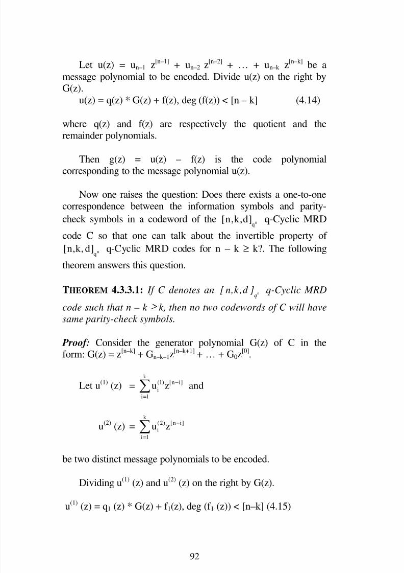
8/2/2019 Erasure Techniques in MRD Codes, by W. B. Vasantha Kandasamy, Florentin Smarandache, R. Sujatha, R. S. Raja …
http://slidepdf.com/reader/full/erasure-techniques-in-mrd-codes-by-w-b-vasantha-kandasamy-florentin-smarandache 93/164
92
Let u(z) = un–1 z[n–1]
+ un–2 z[n–2]
+ … + un–k z[n–k]
be a
message polynomial to be encoded. Divide u(z) on the right byG(z).
u(z) = q(z) * G(z) + f(z), deg (f(z)) < [n – k] (4.14)
where q(z) and f(z) are respectively the quotient and theremainder polynomials.
Then g(z) = u(z) – f(z) is the code polynomialcorresponding to the message polynomial u(z).
Now one raises the question: Does there exists a one-to-onecorrespondence between the information symbols and parity-
check symbols in a codeword of the nq[n,k,d] q-Cyclic MRD
code C so that one can talk about the invertible property of
nq
[n,k, d] q-Cyclic MRD codes for n – k ≥ k?. The following
theorem answers this question.
THEOREM 4.3.3.1: If C denotes an nq
[ n,k ,d ] q-Cyclic MRD
code such that n – k ≥ k, then no two codewords of C will have
same parity-check symbols.
Proof: Consider the generator polynomial G(z) of C in theform: G(z) = z
[n–k]+ Gn–k–1z
[n–k+1]+ … + G0z
[0].
Let u(1)
(z) =k
(1) [n i]
i
i 1
u z−
=
∑ and
u(2)
(z) =k
(2) [n i]
i
i 1
u z−
=
∑
be two distinct message polynomials to be encoded.
Dividing u(1)
(z) and u(2)
(z) on the right by G(z).
u(1) (z) = q1 (z) * G(z) + f 1(z), deg (f 1 (z)) < [n–k] (4.15)

8/2/2019 Erasure Techniques in MRD Codes, by W. B. Vasantha Kandasamy, Florentin Smarandache, R. Sujatha, R. S. Raja …
http://slidepdf.com/reader/full/erasure-techniques-in-mrd-codes-by-w-b-vasantha-kandasamy-florentin-smarandache 94/164
93
and
u(2)
(z) = q2 (z) * G(z) + f 2(z), deg (f 2 (z)) < [n–k]. (4.16)
The code polynomials corresponding to u(1)
(z) and u(2)
(z)
respectively are,
g1(z) = u(1)
(z) – f 1 (z)
and g2(z) = u(2)
(z) – f 2 (z).
Suppose that f 1 (z) = f 2 (z).
Subtracting (4.16) from (4.15),
u(1)
(z) – u(2)
(z) = (q1(z) – q2(z)) * G(z)
i.e., z[n–k]
* (u′(1)(z) – u′(2)
(z)) = (q1(z) – q2(z)) * G(z),
where u(i)
(z) = z[n–k]
* u′(i)(z) for each i = 1, 2.
The above equation shows that G(z) is a right divisor of
z[n–k]
* (u′(1)(z) – u′(2)
(z)). Since z[n–k]
is relatively prime to G(z),
G(z) must be a right divisor of u′(1)(z) – u′(2)
(z). However this is
impossible, because u′(1)(z) ≠ u′(2)
(z) and degree of u′(1)(z) –
u′(2)(z) is less than or equal to [k – 1] but the degree of G(z) is
[n–k] which is strictly greater than [k–1], since n – k ≥ k.
Thus f 1 (z) ≠ f 2(z). Hence the theorem.
Since the remainder f(z) resulting from dividing u(z) byG(z) is unique, the Theorem 4.3.3.1 implies that there exists an
one-to-one correspondence between a message polynomial u(z)
and its parity-check polynomial f(z). Therefore knowing only
the parity-check polynomial f(z), the message polynomial u(z)can be determined uniquely.

8/2/2019 Erasure Techniques in MRD Codes, by W. B. Vasantha Kandasamy, Florentin Smarandache, R. Sujatha, R. S. Raja …
http://slidepdf.com/reader/full/erasure-techniques-in-mrd-codes-by-w-b-vasantha-kandasamy-florentin-smarandache 95/164
94
In what follows, it is shown how to recover the message
polynomial u(z) from its parity-check polynomial f(z). Now onehas the equation (4.14):
u(z) = q(z) * G(z) + f(z), deg(f(z)) < [n–k].
Consider z[k]
* f(z) :
z[k]
* f(z)= z[k]
* (–q(z) * G(z) + u(z))
= z[k]
* (–q(z) * G(z)) + z[k]
* u(z)
= z[k]
* (–q(z) * G(z)) + (u′(z) * z[k]
) * z[n–k]
= z[k]
* (–q(z) * G(z)) + u′(z) * z[n]
= z[k]
* (–q(z) * G(z)) + u′(z) * (z[n]
–z) + u′(z) * z
= (z[k]
* (–q(z))) * G(z) + u′(z) * (H(z)*G(z))+ u′(z)
(since G(z) is a right divisor of z[n] – z).
= (z[k]
* (–q(z)) + u′(z) * H(z)) * G(z) + u′(z),(4.17)
where u′(z) = [k] [k 1]
n 1u z −− + [k] [k 2]
n 2u z −− + … + [k] [0]
n k u z− .
See that from (4.17), the message polynomial u(z) is
nothing but z[n–k] * u′(z);
i.e., u(z) = z[n–k]
* u′(z)
= z[n–k]
*( [k] [k 1]
n 1u z −− + [k] [k 2]
n 2u z −− + … + [k] [0]
n k u z− )
= [k][n k] [n 1]
n 1u z− −− + [k][n k] [n 2]
n 2u z− −− + … + [k][n k] [n k]
n k u z− −−
= [n] [n 1]
n 1u z −− + [n] [n 2]
n 2u z −− + … + [n] [n k ]
n k u z −−

8/2/2019 Erasure Techniques in MRD Codes, by W. B. Vasantha Kandasamy, Florentin Smarandache, R. Sujatha, R. S. Raja …
http://slidepdf.com/reader/full/erasure-techniques-in-mrd-codes-by-w-b-vasantha-kandasamy-florentin-smarandache 96/164
95
= un–1 z[n–1]
+ un–2 z[n–2]
+ … + un–k z[n–k]
,
where u′(z) is nothing but the remainder obtained when
z[k] * f(z) is divided on the right by G(z).
Thus the class of nq
[n,k, d] q-Cyclic MRD codes for
n – k ≥ k are invertible.
An example is given in the following which demonstrates
the invertible property of the 52
[5,2,4] 2-Cyclic MRD code.
Example 4.3.3.1 : Consider the 52
[5,2,4] 2-Cyclic MRD code
generated by G(z) = z8
+ α10z
4+ α17
z2
+ α13z, where α is a root
of the primitive polynomial x5
+ x2
+ 1 over GF(2).
The generator matrix G and the parity-check matrix H for
the 52[5,2,4] 2-Cyclic MRD code in systematic form are
respectively given by
G =13 17 10
2 14 9
1 0
0 1
α α α
α α α
and
H =
13 2
17 14
10 9
1 0 0
0 1 0
0 0 1
α α
α α α α
.
Let u1(z) = z16
+ αz8
be the message polynomial to be
encoded.
Dividing u1(z) on the right by G(z), one obtains
z16
+ αz8
= (z2
+ α12z) * G(z) + f 1(z),
where f 1 (z) = α14 z4 + α24 z2 + α25 z.

8/2/2019 Erasure Techniques in MRD Codes, by W. B. Vasantha Kandasamy, Florentin Smarandache, R. Sujatha, R. S. Raja …
http://slidepdf.com/reader/full/erasure-techniques-in-mrd-codes-by-w-b-vasantha-kandasamy-florentin-smarandache 97/164
96
Dividing z[2]
* f 1(z) on the right by G(z), one obtains
α25z
16+ α3
z8
+ α7z
4= (α25
z2
+ α22z) + G(z) + 1f (z)′ ,
where 1f (z)′ = z2
+ α4z. Then the message polynomial u1(z) is
z[3]
* (z2
+ α4z) = z
16+ αz
8.
Thus the message polynomial u1(z) = z16
+ αz8
is obtainedonly with the knowledge of the parity-check polynomial
f 1(z) = α14z
4+ α24
z2
+ α25z.
Similarly, the message polynomial u2(z) = z8 can beobtained from the parity-check polynomial
f 2(z) = α10z
4+ α17
z2
+ α13z, as the remainder obtained by
dividing z[2]
* f 2(z) on the right by G(z) is 2f (z)′ = z and thus
u2 (z) = z[3]
* 2f (z)′ .
The case when n–k < k, the q-Cyclic MRD codes are not
invertible, but the class of shortened n0 0q
[n t ,k t ]− − q-Cyclic
MRD codes, 2k–n ≤ t0 < k has the invertible property which isproved in what follows.
Case (ii) n – k < k
The case when n – k < k, the class of nq
[n,k,d] q-Cyclic
MRD codes are not invertible. But the codes obtained by
shortening the nq[n,k,d] q-Cyclic MRD codes by removing the
t0 leading zero information symbols are invertible, where 2k – n
≤ t0 < k; i.e., the shortened n0 0 q[n t ,k t ]− − q-Cyclic MRD
codes are invertible.
Following example shows the face that an nq[n,k,d] q-
Cyclic MRD code with n – k < k is not invertible.

8/2/2019 Erasure Techniques in MRD Codes, by W. B. Vasantha Kandasamy, Florentin Smarandache, R. Sujatha, R. S. Raja …
http://slidepdf.com/reader/full/erasure-techniques-in-mrd-codes-by-w-b-vasantha-kandasamy-florentin-smarandache 98/164
97
Example 4.3.3.2: Consider GF (33) = {0, 1, a, …,
33 2−α },
where α is a root of the primitive polynomial x3
+ 2x + 1 over
GF(3). Let C = 33[3,2,2] be the 3-Cyclic MRD code with thegenerator polynomial G(z) = z
3+ α21
z.
The generator matrix G and the parity-check matrix H for
the 33
[3,2,2] 3-Cyclic MRD code in systematic form are
respectively given by
G =
8
6
1 0
0 1
α
α and H = [1 –α8
–α6
].
Let u(z) = α22z
9+ α7
z3
be a message polynomial.
Dividing u(z) on the right by G(z), one obtains
α22z
9+ α7
z3
= α22z
3* G(z) + f(z),
where f(z) ≡ 0, the zero polynomial.
Then dividing z[2]
* f (z) on the right by G(z), one obtains
the remainder polynomial u′(z) ≡ 0 so that z[1]
* u′(z) ≡ 0; but
u(z) = α22z
9+ α7
z3, which is not the zero polynomial.
Thus from the parity-check polynomial f(z), the message
polynomial u(z) is not retrieved. This is because the parity block
is same for the codewords (0, 0, 0) and (0, α7, α22).
Thus an nq[n,k,d] q-Cyclic MRD code for which n – k < k
need not be invertible.
Using the shortening technique to the class of nq[n,k,d]
q-Cyclic MRD codes discussed in subsection 4.3.2, one can
obtain a class of invertible shortened n0 0 q[n t ,k t ]− − q-CyclicMRD codes as follows, 2k – n ≤ t0 < k.

8/2/2019 Erasure Techniques in MRD Codes, by W. B. Vasantha Kandasamy, Florentin Smarandache, R. Sujatha, R. S. Raja …
http://slidepdf.com/reader/full/erasure-techniques-in-mrd-codes-by-w-b-vasantha-kandasamy-florentin-smarandache 99/164
98
Let C denote an nq
[n,k,d] q-Cyclic MRD code generated
by G(z) =n k [i]
ii 0G z
−
=∑ such that n – k < k. Let H(z) =
k [i ]
ii 0H z
=∑ be such that z[n] – z = H(z) * G(z). Let t0 be such
that 2k – n ≤ t0 < k.
Consider the shortened n0 0 q[n t ,k t ]− − q-Cyclic MRD code
0( )t C of length n – t0 and dimension k – t0. The encoding
scheme, similar to the nq[n,k,d] q-Cyclic MRD code C, for the
shortened n0 0 q[n t ,k t ]− − q-Cyclic MRD code 0( )t C is given
below.
Let u(z) = 0 0
0 0
[( ) 1] [( ) 2] [ ]
1 2 ...n t n t n k
n t n t n k u z u z u z− − − − −
− − − − −+ + +
be a message polynomial to be encoded. Divide u(z) on the rightby G(z):
u(z) = q(z) * G(z) + f(z), deg (f(z)) < [n – k], (4.18)where q(z) and f(z) are respectively the quotient and the
remainder polynomials.
Then g(z) = u(z) – f(z) is the code polynomialcorresponding to the message polynomial u(z).
Now one needs to ensure that no two codewords in the
shortened n0 0 q[n t ,k t ]− − q-Cyclic MRD code
0( )t C have same
parity block. This is proved in the following theorem. Thoughthe proof is similar to the case (i), here it is given for the sake of
completeness.
THEOREM 4.3.3.2: Let C be an nq
[n,k ,d ] q-Cyclic MRD code
such that n – k < k. Let 0( )t C be the shortened 0 0 n
q[ n t ,k t ]− −
q-Cyclic MRD code, 2k – n ≤ t 0 < k. Then no two codewords of
0( )t C will have same parity-check symbols.

8/2/2019 Erasure Techniques in MRD Codes, by W. B. Vasantha Kandasamy, Florentin Smarandache, R. Sujatha, R. S. Raja …
http://slidepdf.com/reader/full/erasure-techniques-in-mrd-codes-by-w-b-vasantha-kandasamy-florentin-smarandache 100/164
99
Proof: Consider the generator polynomial G(z) of C in the
form: G(z) = z[n–k]
+[ 1]
1
n k
n k G z − +− − + … + G0z
[0].
Let u(1)
(z) =0
0
k t[n t i](1)
i
i 1
u z−
− −
=∑ and
u(2)
(z) =0
0
k t[n t i](2)
i
i 1
u z−
− −
=∑
be two distinct message polynomials to be encoded.
Dividing u(1)
(z) and u(2)
(z) on the right by G(z),
u(1)
(z) = q1 (z) * G(z) + f 1(z), deg (f 1 (z)) < [n–k] [4.19]
and u(2)
(z) = q2 (z) * G(z) + f 2(z), deg (f 2 (z)) < [n–k]
[4.20]
The code polynomials corresponding to u(1)
(z) and u(2)
(z)respectively are,
g1(z) = u(1)
(z) – f 1(z)
and g2(z) = u(2)
(z) – f 2(z).
Suppose that f 1(z) = f 2(z).
Subtracting (4.20) from (4.19),
u(1)
(z) – u(2)
(z) = (q1(z) – q2(z)) * G(z)
i.e., z[n–k]
* (u′(1)(z) – u′(2)
(z)) = (q1(z) – q2(z)) * G(z),
where u′(1), u′(2)
are such u(1)
(z) = z[n–k]
* u′(1)(z) and
u
(2)
(z) = z
[n–k]
* u′
(2)
(z).

8/2/2019 Erasure Techniques in MRD Codes, by W. B. Vasantha Kandasamy, Florentin Smarandache, R. Sujatha, R. S. Raja …
http://slidepdf.com/reader/full/erasure-techniques-in-mrd-codes-by-w-b-vasantha-kandasamy-florentin-smarandache 101/164
100
This shows that G(z) is a right divisor of
z[n–k]
* (u′(1)(z) – u′(2)
(z)).
Since z[n–k] is relatively prime to G(z), G(z) is a right divisorof u′(1)
(z) – u′(2)(z).
However this is impossible, because u′(1)(z) – u′(2)
(z) ≠ 0 andits degree is less than [k–t0–1] but the degree of G(z) is [n – k]
which is strictly great than [k–t0–1].
Thus f 1 (z) ≠ f 2(z). Hence the theorem.
Since the remainder f(z) resulting from dividing u(z) by
G(z) is unique, the Theorem 4.3.3.2 implies that there exists an
one-to-one correspondence between a message polynomial u(z)and its parity-check polynomial f(z). Therefore knowing only
the parity-check polynomial f(z) alone, the message polynomial
u(z) can be determined uniquely.
In what follows, it is shown how to recover the message
polynomial u(z) from its parity-check polynomial f(z). Now onehas the equation (4.18):
u(z) = q(z) * G(z) + f(z), deg(f(z)) < [n–k].
Consider z[k]
* f(z) :
z[k]
* f(z) = z[k]
* (–q(z) * G(z) + u(z))
= z[k]
* (–q(z) * G(z)) + z[k]
* u(z)
= z[k]
* (–q(z) * G(z)) + (u′(z) * z[k]
) * z[n–k]
= z[k]
* (–q(z) * G(z)) + u′(z) * z[n]
= z[k]
* (–q(z) * G(z)) + u′(z) * (z[n]
–z) + u′ (z) * z
= (z[k] * (–q(z))) * G(z) + u′(z) * (H(z)*G(z))+ u′(z)

8/2/2019 Erasure Techniques in MRD Codes, by W. B. Vasantha Kandasamy, Florentin Smarandache, R. Sujatha, R. S. Raja …
http://slidepdf.com/reader/full/erasure-techniques-in-mrd-codes-by-w-b-vasantha-kandasamy-florentin-smarandache 102/164
101
(since G(z) is a right divisor of z[n]
– z).
= (z[k]
* (–q(z)) + u′(z) * H(z)) * G(z) + u′(z), (4.21)
where u′(z) = 0
0
[k t 1][k ]
n t 1u z− −
− − + 0
0
[k t 2][k]
n t 2u z− −
− − + … + [k] [0]
n k u z− .
See that from (4.21), the message polynomial u(z) is
nothing but z[n–k]
* u′(z);
i.e., u(z) = z[n–k]
* u′(z)
= z[n–k] *( 0
0
[k t 1][k ]n t 1u z − −
− − + 0
0
[k t 2][k]n t 2u z − −
− −
+ … + [k] [0]
n k u z− )
= 0
0
[n t 1][k][n k]
n t 1u z− −−
− − + 0
0
[n t 2][k][n k]
n t 2u z− −−
− −
+ … + [k][n k] [n k]
n k u z− −−
= 0
0
[n t 1][n ]
n t 1u z
− −
− −+ 0
0
[n t 2][n]
n t 2u z
− −
− −+ … + [n] [n k ]
n k u z −
−
= 0
0
[n t 1]
n t 1u z− −
− − + 0
0
[n t 2]
n t 2u z− −
− − + … + [n k ]
n k u z −− ,
where u′(z) is nothing but the remainder obtained whenz
[k]* f(z) is divided on the right by G(z).
Having carried out a comprehensive study on a
characteristic of RD codes, namely the invertible property of theclass of RD codes, the next section deals yet anothercharacteristic enjoyed by the class of RD codes: Rank Distance
codes having complementary duals.
4.4 Rank Distance Codes With Complementary Duals
It is known that an (n, k) F-ary linear code is just a k-
dimensional subspace of the n-dimensional vector space Fn
of n-tuples with coordinates in the finite field F. Recall that the
vectors u and v in Fn
are said to be orthogonal if ⟨u, v⟩ = 0 and

8/2/2019 Erasure Techniques in MRD Codes, by W. B. Vasantha Kandasamy, Florentin Smarandache, R. Sujatha, R. S. Raja …
http://slidepdf.com/reader/full/erasure-techniques-in-mrd-codes-by-w-b-vasantha-kandasamy-florentin-smarandache 103/164
102
that, if Γ is an (n, k) F-ary linear code, the dual code Γ ⊥ is the
(n, n–k) F-ary linear code consisting of all vectors v ∈ Fn
that
are orthogonal to every vector u in Γ . The class of Linear codes
with Complementary Duals (LCD codes) is defined by J.L.Massey [19] in 1992. A F-ary linear code Γ is called an LCD
code if Γ ∩ Γ ⊥ = {0}. It is immediate that Γ is an LCD code justwhen the following occurs
Fn
= Γ ⊕ Γ ⊥ ;
that is, when Fn
is the direct sum of Γ and Γ ⊥.
The following theorem due to J.L. Massey [19] gives analgebraic characterization to the class of LCD codes.
THEOREM 4.4.1: [19] Let Γ be an (n, k) F-ary linear code with
generator matrix G. Then Γ is an LCD code if and only if the k
× k matrix GGT
is non-singular. Further, if Γ is in LCD code,
then ∏ Γ = GT
(GGT ) –1
G is the orthogonal projector from F n
onto Γ .
Recall that the trace function tr : GF(2n) → GF(2) is defined
by tr(a) =n 1 2 j
j 0a
−
=∑ . Let B = {b1, b2, …, bn} be an ordered basis
of GF(2n) over GF(2) and 1 2 n{b , b ,..., b } be the dual basis of B
with respect to the trace function, i.e.,
tri j
(b b ) = δij
for 1 ≤ i, j ≤ n, where δij
is the Kronecker’s
symbol. Then B is called trace-orthogonal if bi = ib , 1 ≤ i ≤ n.
The dual basis of any basis of GF (2n) over GF (2) is determined
uniquely [20, Theorem 4.1.1]. It is known that a trace-
orthogonal basis of GF(2n) over GF(2) exists for any positive
integer n [23].
This section carries out a brief study on the class of
n2[n,k, d] Rank Distance codes having complementary duals.

8/2/2019 Erasure Techniques in MRD Codes, by W. B. Vasantha Kandasamy, Florentin Smarandache, R. Sujatha, R. S. Raja …
http://slidepdf.com/reader/full/erasure-techniques-in-mrd-codes-by-w-b-vasantha-kandasamy-florentin-smarandache 104/164
103
Consider the generator matrix of an n2[n,k,d] MRD code:
G =
1 2 n[1] [1] [1]
1 2 n
[k 1] [k 1] [k 1]
1 2 n
...
...
...− − −
α α α α α α α α α
(4.22)
where α1, α2, …, αn are linearly independent over GF(2).
Represent the generator matrix G defined as in (4.22) by
G =k 1,n
2i
j i, j 0,1
−
= α where α1, α2, …, αn are linearly independent
GF(2). This book calls the matrix G =k 1,n
2i
j i, j 0,1
−
= α with the first
row entries α1, α2, …, αn being a trace-orthogonal basis inGF(2
n) as the trace-orthogonal-generator matrix. Clearly, G
generates an n2[n,k,d] MRD code.
This section is divided into three subsections. Thesubsection 1 proves that the class of n2
[n,k,d] MRD codes
generated by the trace-orthogonal-generator matrices are LCD
codes. Description to the (noiseless and noisy) 2-user F-Adder
Channel is given in subsection 2. The final subsection gives thecoding for the noiseless 2-user F-Adder Channel via the class of
n2
[n,k,d] MRD codes having complementary duals and
describes a coding problem with the noisy 2-user F-AdderChannel.
4.4.1 MRD Codes with Complementary Duals
It is observed that an nq[n,k,d] RD code, n ≤ N with
d < n – k + 1 need not be an LCD code but it is interesting to see
that the class of n2
[n,k,d] MRD codes generated by the trace-
orthogonal-generator matrices are LCD codes.

8/2/2019 Erasure Techniques in MRD Codes, by W. B. Vasantha Kandasamy, Florentin Smarandache, R. Sujatha, R. S. Raja …
http://slidepdf.com/reader/full/erasure-techniques-in-mrd-codes-by-w-b-vasantha-kandasamy-florentin-smarandache 105/164
104
The following counter example shows that an nq[n, k, d] RD
code, n ≤ N with d < n – k + 1 need not be an LCD code.
Example 4.4.1.1: Let GF (23) = {0, 1, α, α2
, α3, α4
, α5, α6
},
where α is a root of the primitive polynomial x3
+ x + 1 overGF(2).
Let Γ = 32[3,2,1] be the 2-Cyclic RD code with the generator
matrix G corresponding to the generator polynomial
G(Z) = z2
+ αz is given as
G =2
1 0
0 1
α α
.
Clearly |GGT| = (0). Thus the 32
[3,2,1] 2-Cyclic RD code is
not an LCD code.
The following theorem proves that an n
2
[n,k,d] MRD code
generated by a trace-orthogonal-generator matrix is an LCD
code.
THEOREM 4.4.1.1: An2n[ n,k,d ] MRD code generated by
G =1
2
0 1
k ,ni
ji , j ,
−
= α with {α 1 , α 2 , …, α n } being a trace-orthogonal
basis in GF(2n) is an LCD code.
Let Γ denote an n2[n,k,d] MRD code generated by
G =
1 2 n
[1] [1] [1]
1 2 n
[k 1] [k 1] [k 1]
1 2 n
...
...
...− − −
α α α α α α α α α
,
where {α1, α2, …, αn} is a trace-orthogonal basis in GF(2n).

8/2/2019 Erasure Techniques in MRD Codes, by W. B. Vasantha Kandasamy, Florentin Smarandache, R. Sujatha, R. S. Raja …
http://slidepdf.com/reader/full/erasure-techniques-in-mrd-codes-by-w-b-vasantha-kandasamy-florentin-smarandache 106/164
105
In order to prove that Γ is an LCD code, one has to prove
that the k × k matrix GGT
is non-singular.
Since {α1, α2, …, αn} is a trace-orthogonal basis in GF(2n),
the k row vectors 2i 2i 2i
1 2 n( , ,..., )α α α , i = 0, 1, …, k–1 are
orthonormal vectors. It follows that GGT
= I, where
I denotes the identity matrix. Thus, GGT
is non-singular.
Therefore, Γ is an LCD code.
Further, the orthogonal projector ∏Γ from [GF(2n)]
nonto Γ
defined by r∏Γ = rGT(GG
T)
-1G for each r ∈ [GF(2
n)]
nexists.
In the above theorem, it is proved that the class of n2[n,k,d]
MRD codes generated by the generator matrices of the form
G =i k 1,n
2
ji, j 0,1
−
=
α with {α1, α2, …, αn} being a trace-orthogonal
basis in GF(2n) are LCD codes. But there exists N
q[n, k,d] MRD
codes, n ≤ N generated by generator matrices of the form G =
i k 1,nq
ji, j 0,1
−
= α with the first row entries α1, α2, …, αn are linearly
independent over GF(q) are LCD codes. This is evident fromthe following example.
Example 4.4.1.2: Let Γ =3
[3,1,3] be the MRD code with the
generator matrix G :
G = [α4 α65
1],
where α is a root of the primitive polynomial x4
+ x + 2 over
GF(3). Clearly |GGT| ≠ (0).
The class of n2[n,k,d] MRD codes having complementary
duals is effective at coding over the noiseless 2-user F-Adder
Channel, which can be seen in the next subsection.

8/2/2019 Erasure Techniques in MRD Codes, by W. B. Vasantha Kandasamy, Florentin Smarandache, R. Sujatha, R. S. Raja …
http://slidepdf.com/reader/full/erasure-techniques-in-mrd-codes-by-w-b-vasantha-kandasamy-florentin-smarandache 107/164
106
4.4.2 The 2-user F-Adder Channel
Given a finite field F, the F-Adder Channel is described as
the channel whose inputs are elements of F and the output is thesum (over F) of the inputs [25]. This section describes 2-user F-
Adder Channel as the F-Adder Channel shared by 2 users.Following are the descriptions to the 2-user F-Adder Channel,
for both the noiseless and noisy cases.
Case (i) Noiseless 2-user F-Adder Channel
A pictorial representation of the noiseless 2-user F-AdderChannel is depicted in the following figure. In this noiseless
communication channel, the two users of the 2-user F-Adder
Channel transmit two n-tuples, say γ 1 and γ 2 respectively from
the F-ary linear codes Γ 1 and Γ 2. Then the received vector, say r
is the componentwise sum γ 1 + γ 2 over the finite field F.
Noiseless 2-user F-Adder Channel
In this noiseless channel, the problem for the receiver is to
decode the received vector r = γ 1 + γ 2 into the codewords γ 1 and
γ 2 originally transmitted. The next subsection provides a
solution to this problem through the class of n2[n,k,d] MRD
codes having complementary duals.
+r = γ 1 + γ 2
1
γ 2

8/2/2019 Erasure Techniques in MRD Codes, by W. B. Vasantha Kandasamy, Florentin Smarandache, R. Sujatha, R. S. Raja …
http://slidepdf.com/reader/full/erasure-techniques-in-mrd-codes-by-w-b-vasantha-kandasamy-florentin-smarandache 108/164
107
Case (ii) Noisy 2-user F-Adder Channel
Consider the pictorial representation of the noisy 2-user F-Adder Channel depicted in the following figure in which the
two users are attempting to transmit two
Noisy 2-user F-Adder Channel
codewords, say γ 1 and γ 2 respectively from the F-ary linear
codes Γ 1 and Γ 2. Then, in this noisy channel, the receivedvector, say r′ is the componentwise sum γ 1 + γ 2 + e over F,where e is an error-vector. The problem for the receiver is to
decode the received vector r′ = γ 1 + γ 2 + e into the transmitted
codewords γ 1 and γ 2.
4.4.3 Coding for the 2-user F-Adder Channel
As described in the previous subsection, the 2-user F-AdderChannel is a F-Adder Channel shared by 2 users. This
subsection describes how the class of n2[n,k,d] MRD codes
having complementary duals can be effectively used over the
noiseless 2-user GF(2n) - Adder Channel. For the case when the
2-user F-Adder Channel is noisy, the coding problem isdescribed. It is observed that the class of LCD codes is not
suitable for coding over the noisy 2-user F-Adder Channel.
+
r′ = γ 1 + γ 2 + e
γ 1
γ 2

8/2/2019 Erasure Techniques in MRD Codes, by W. B. Vasantha Kandasamy, Florentin Smarandache, R. Sujatha, R. S. Raja …
http://slidepdf.com/reader/full/erasure-techniques-in-mrd-codes-by-w-b-vasantha-kandasamy-florentin-smarandache 109/164
108
Case (i) Noiseless 2-user F-Adder Channel
Consider the pictorial representation of the noiseless 2-user
F-Adder Channel given in figure for F = GF (2n). Let Γ be ann2
[n, k] MRD code generated by a trace-orthogonal-generator
matrix and Γ ⊥ = n2
[n,n k]− denote its dual code. Assume that
the two users of the noiseless 2-user GF(2n)-Adder Channel
transmit the codewords γ and β from Γ and Γ ⊥ respectively.Then, in this noiseless 2-user GF(2
n) - Adder Channel, the
received vector r is the componentwise sum γ + β over GF(2n).
Since Γ is an LCD code, the orthogonal projector
∏Γ = GT (GGT)
–1G defined from [GF(2
n)]
nonto Γ exists. To
receive the codewords γ and β, the receiver simply applies the
orthogonal projector ∏Γ on r which gives r∏Γ = γ . The
codeword β is then obtained by subtracting γ from r = γ + β.
Thus the codewords γ and β transmitted are retrieved from thereceived vector r successfully.
The following example describes the coding for the
noiseless 2-user GF(34)-Adder Channel via
3[3,1,3] MRD code.
Example 4.4.3.1: Let Γ =3
[3,1,3] be the 3-Cyclic MRD code
with the generator matrix G and parity-check matrix H.
G = [α
4
α
65
1] and H =
2
3 6
1
1
α α
α α ,
where α is a root of the primitive polynomial x4
+ x + 2 over
GF(3). Note that the generator matrix for the dual code Γ ⊥ is H.
Since Γ being an LCD code, the orthogonal projector ∏Γ
defined from [GF (34)]
4onto Γ is given by

8/2/2019 Erasure Techniques in MRD Codes, by W. B. Vasantha Kandasamy, Florentin Smarandache, R. Sujatha, R. S. Raja …
http://slidepdf.com/reader/full/erasure-techniques-in-mrd-codes-by-w-b-vasantha-kandasamy-florentin-smarandache 110/164
109
∏Γ =
41 22 37
22 3 18
37 18 33
α α α α α α
α α α
.
Suppose the codewords γ 1 = (1, α61, α76
) and
γ 2 = (α2, α5
, α8) from Γ and Γ ⊥ respectively be transmitted over
the noiseless 2-user GF (34)-Adder Channel. Then r = γ 1 + γ 2 =
(α24, α78
, α35) is the received vector.
Applying the orthogonal projector ∏Γ on r:
γ 1 = (α24, α78
, α35) ∏Γ = (1, α61
, α76).
Then γ 2 = r – (1, α61, α76
) = (α2, α5
, α8). Hence the
codewords γ 1 = (1, α61, α76
) and γ 2 = (α2, α5
, α8) are retrieved
from r = (α24, α78
, α35).
Case (ii) Noisy 2-user F-Adder Channel
Consider the pictorial representation of the noisy 2-user F-
Adder Channel depicted in figure.
In this noisy channel, the received vector r′ may not always
be the sum of the transmitted codewords γ 1 and γ 2, but may be a
sum of the transmitted codewords along errors, i.e., r′ = γ 1 + γ 2 +
e, where e is an error-vector. Let r[e; q] ≤ d 1
2
−
with d being
a positive integer.
The problem here for the decoder is to employ an error-
correcting decoding scheme to decode the received vector r′. If one employs the coding scheme described for the noiseless case
s/he would not recover the transmitted codewords γ 1 and γ 2 from
the erroneously received vector r′. Suppose Γ is an LCD code
such that γ 1 ∈ Γ , γ 2 ∈ Γ ⊥
, then γ 1 + γ 2 ∈ F
n
= Γ ⊕ Γ ⊥
so thaterror correction is not possible in the erroneously received

8/2/2019 Erasure Techniques in MRD Codes, by W. B. Vasantha Kandasamy, Florentin Smarandache, R. Sujatha, R. S. Raja …
http://slidepdf.com/reader/full/erasure-techniques-in-mrd-codes-by-w-b-vasantha-kandasamy-florentin-smarandache 111/164
110
vector r′ = γ 1 + γ 2 + e. Consider a situation wherein γ 1 + γ 2 is acodeword of an (n, k, d) F-ary linear code with the parity-check
matrix H. Then employing the associated error-correcting
decoding technique and using the syndrome r′HT, one candecode the received vector r′ into γ 1 and γ 2.
If this is the situation, one can correct uptod 1
2
−
errors in
the erroneously received vector r′. So, the prime motivation is toconstruct multiuser error-correcting codes that can be employed
over the noisy 2-user F-Adder Channel effectively.

8/2/2019 Erasure Techniques in MRD Codes, by W. B. Vasantha Kandasamy, Florentin Smarandache, R. Sujatha, R. S. Raja …
http://slidepdf.com/reader/full/erasure-techniques-in-mrd-codes-by-w-b-vasantha-kandasamy-florentin-smarandache 112/164
111
Chapter Five
EFFECTIVE ERASURE CODES FOR
R ELIABLE COMPUTER COMMUNICATION
PROTOCOLS USING CODES OVER
ARBITRARY INTEGER RINGS
Linear algebraic codes can be defined using symbols chosenfrom a set of arbitrary size. However, most of the results of
coding theory have been derived assuming that the code
symbols are elements of a finite field especially the finite fieldZ2 = {0, 1}. Recently linear codes over integer rings have raised
a great interest for their role in algebraic coding theory and their
successful applications in combined coding and modulation. [2,3] has constructed cyclic codes over Zm (the ring of integers
modulo m) where m is an interger of the form p1, p2, …, pk
where pi’s are distinct primes, from cyclic codes overipZ . In
his later paper, Blake derived parity check matrices for codes
over Zm analogous to Hamming codes and Reed-Solomoncodes. Calderbank and Sloane [4], Priti Shanker [23], J.C.
Interlando et al [13] extended the notion of cyclic codes, Reed-
Solomon codes and BCH codes over GF(q) to class of codesover finite rings Zq, with q a power of a prime. Most studies in

8/2/2019 Erasure Techniques in MRD Codes, by W. B. Vasantha Kandasamy, Florentin Smarandache, R. Sujatha, R. S. Raja …
http://slidepdf.com/reader/full/erasure-techniques-in-mrd-codes-by-w-b-vasantha-kandasamy-florentin-smarandache 113/164
112
algebraic coding theory deal with Hamming metric. Since the
Hamming metric is not always well matched to thecharacteristics of the real channels EM. Gabidulin [9]
introduced a new metric, called the rank metric, and he calledthe codes equipped with this metric as rank distance codes.
In this chapter we study the codes with rank metric over the
ring of integers modulo 2m, where 2m = 2p1, p2, …, pt, where
pi’s are distinct primes. These codes are proved to be better thanthe codes with Hamming metric as they can cater to the
complex and unpredictable situations in the communicating
channels. Further, they are found to have a better errorcorrecting capability.
This chapter is divided into two sections. In the first section
we define a new class of codes, called the integer rank distancecodes using the ring of integers modulo 2m. In the second
section we define the Maximum Integer Rank Distance codes
(MIRD codes) using the main result - Singleton - style boundfor integer rank distance codes. Further we give the method of
coding and decoding algorithm for this new class of MIRDcodes without which the construction will not be complete.
5.1. Integer Rank Distance Code
As said earlier Z2m is the ring of integers modulo 2m where
2m = 2p1 p2… pt, where pi’s are distinct primes. Let Z2m [x] be
the ring of polynomials in the indeterminate x. Let p(x) ∈ Z2m[x] be an irreducible polynomial of degree n over Z2m. Let V
be Z2m[x] / ⟨p (x)⟩, where ⟨p(x)⟩ denotes the ideal generated by p(x). Clearly V is a module of dimension n over Z2m. Any
element x ∈ V can be represented by x = (x1, x2, …, xn) where xi
∈ Z2m i.e., a polynomial is regarded as a n-tuple. The elementsof Z2m can be treated as polynomials in 2 over Z2. Hence an
element x1 ∈ Z2m has representation as a N0-tuple
( )0i1i 2i Nx ,x ,..., x , xij ∈ Z2. Hence, with each x ∈ V we have an
associated matrix,

8/2/2019 Erasure Techniques in MRD Codes, by W. B. Vasantha Kandasamy, Florentin Smarandache, R. Sujatha, R. S. Raja …
http://slidepdf.com/reader/full/erasure-techniques-in-mrd-codes-by-w-b-vasantha-kandasamy-florentin-smarandache 114/164
113
m(x) =
0 0 0
11 12 1n
21 22 2n
N 1 N 2 N n
x x ... x
x x ... x
x x ... x
where the i-th column represents the i-th coordinate ‘x i’ of ‘x’
over Z2.
DEFINITION 5.1.1: Rank of an element x ∈ V is defined as the
rank of the matrix m(x) over Z 2.
Let n(x) denote the rank of the m(x). Then it is clear that the
function x → r 1(x) is a norm on V. We call this as the integer
rank norm and denote this by r 1(x). The metric induced by the
integer rank norm is defined as the integer rank metric on V.
If x, y ∈ V, then the integer rank distance between x and y is
d 1(x, y) = r 1 (x + y).
We illustrate this by an example.
Example 5.1.1: Let V = Z6[x] / ⟨x3+ 1⟩. Then, V is a module
over Z6 and the elements of Z6 can be treated as polynomials in
2 over Z2. Let x = (3, 5, 2) ∈ V.
Then, m(x) =
0 1 0
1 0 1
1 1 0
over Z2.
Clearly rank of m(x) is 3.
DEFINITION 5.1.2: The module equipped with this integer rank
metric, for convenience we call it as the integer rank distance
space.
DEFINITION 5.1.3: A linear (n, k) integer rank distance code isa linear submodule of dimension k in the integer rank distance
space V.

8/2/2019 Erasure Techniques in MRD Codes, by W. B. Vasantha Kandasamy, Florentin Smarandache, R. Sujatha, R. S. Raja …
http://slidepdf.com/reader/full/erasure-techniques-in-mrd-codes-by-w-b-vasantha-kandasamy-florentin-smarandache 115/164
114
By C(n, k), we denote a linear (n, k) integer rank distance
code. Let d = min {d 1 (x, y) : x, y ∈ C(n, k)}. This d is called the
minimum integer rank distance of the integer rank distance
code C(n, k). Now C(n, k) is a linear (n, k, d) integer rank distance code.
DEFINITION 5.1.4: A generator matrix G of a linear (n, k)
integer rank distance code C(n, k) is a k × n matrix over Z 2m
whose rows form a basis for C(n, k). We can reduce the
generator matrix G to the form G = [I k , Ak, n–k ] where I k is the k
× k identity matrix and Ak, n–k is some k × (n–k) matrix over Z 2m.
DEFINITION 5.1.5: If G is a generator matrix of a linear (n, k)
integer rank distance code C[n, k], then a matrix H of order
(n – k) × n over Z 2m such that GH T
= {0} is called a parity check
matrix of C[n, k].
H can be reduced to the form H =T
(n k ) k n k A ,I− × − − .
We define a linear (n, k) integer rank distance code as :
1. The linear submodule generated by the rows of the
generator matrix (or)
2. the solution space of the parity check matrix.
Note: The usual Hamming distance between any two vectors, x,
y ∈ V, which is the number of places in which x and y differ
also induces a norm on each vector x ∈ V, called the Hammingnorm, which is denoted throughout this paper as rH(x).
5.2. Maximum Integer Rank Distance Codes
In this section we mainly arrive at a singleton - style bound
for integer rank distance codes, using which we defineMaximum Integer Rank Distance codes, which we refer by
MIRD codes here after. To achieve this we essentially make use
of the following lemma. Further, we give a characterization

8/2/2019 Erasure Techniques in MRD Codes, by W. B. Vasantha Kandasamy, Florentin Smarandache, R. Sujatha, R. S. Raja …
http://slidepdf.com/reader/full/erasure-techniques-in-mrd-codes-by-w-b-vasantha-kandasamy-florentin-smarandache 116/164
115
theorem for finding the maximum integer rank distance of a
integer rank distance code.
Lemma 5.2.1: Let n1 and n2 be any two norms defined on Vwith n1(x) ≤ n2(x), for all x ∈ V. Let V1(n, d) and V2(n, d) be thevolumes of codes with maximum distance d with norms n1 and
n2, respectively. Then, V1(n, d) ≤ V2(n, d).
Proof : Since n1(x) ≤ n2(x), for all x ∈ V, any y ∈ V1(n, d) willalso be in V2 (n, d).
Hence V1(n, d) ≤ V2(n, d).
THEOREM 5.2.1: (Singleton-style bound for integer rank
distance codes) Any linear (n, k, d) integer rank distance code
satisfies the inequality d ≤ n – k + 1.
Proof : Choosing n1 = r1(x) and n2 = rH(x), we have r1(x) ≤ rH(x), we have by Lemma 5.2.1 and the singleton bound for
codes over integer rings with Hamming metric, d ≤ n–k+1.
DEFINITION 5.2.1: Codes which attain equality in the singleton-
style bound are called Maximum Integer Rank Distance codes
(MIRD codes).
The following theorem is used to find the minimum integerrank distance of the linear (n, k) integer rank distance code.
THEOREM 5.2.2: Let C be a linear (n, k) integer rank distancecode with generator matrix G and parity check matrix H. Then,
C has rank distance d if and only if for any (d – 1) × n matrix M
of rank d–1 with elements from Z 2 ,
r(MH T ; Z 2m) = d – 1 (5.2.1)
and then there exists a d × n matrix M 1 of rank d with elements
from Z 2 for which
r(M 1 H T ; Z 2m) < d (5.2.2)

8/2/2019 Erasure Techniques in MRD Codes, by W. B. Vasantha Kandasamy, Florentin Smarandache, R. Sujatha, R. S. Raja …
http://slidepdf.com/reader/full/erasure-techniques-in-mrd-codes-by-w-b-vasantha-kandasamy-florentin-smarandache 117/164
116
Proof : Let x = (x1, x2, …, xn) be any vector in V such that
r1(x) ≤ d. Then, there exists a matrix M1 such that x = zM1,
where z = (z1, z2, …, zd), zi ∈ Z2m, i = 1, 2, …, d and M1 is ad × n matrix of rank d with elements from Z2. Assume that codeC contains a codeword x with rank d. Then, xH
T= (0), which
implies zM1HT
= (0). Consequently, r(M1HT; Z2m) < d. Since the
codes has minimum distance d for any (d – 1) × n matrix N of rank d – 1 with elements from Z2, the equation
(z1, z2, …, zd-1) MHT
= (0) (5.2.3)
should have only a trivial solution i.e.,
r(MHT; Z2m) < d.
Sufficient part is direct from the definition.
THEOREM 5.2.3: A code C is a linear MIRD (n, k) code if and
only if for any (n–k) × n matrix M of rank n – k with elements
from Z 2;r(MH
T ; Z 2m) = n–k (5.2.4)
Proof: From theorem 5.2.1 we get d ≤ n – k +1. By theorem
5.2.1, n – k + 1 ≥ d. Therefore, d = n – k + 1.
We define a class of MIRD codes of length n ≤ N0. These
codes are analogous to the generalized Reed-Solomon codes
over integer rings.
We introduce the notation [i] = 2i; i = 0, ± 1, ± 2, …
Assume that hi ∈ Z2m, i = 1, 2, …, n and assume that theseelements are linearly independent over Z2. Given the designeddistance d < n, we generate the matrix
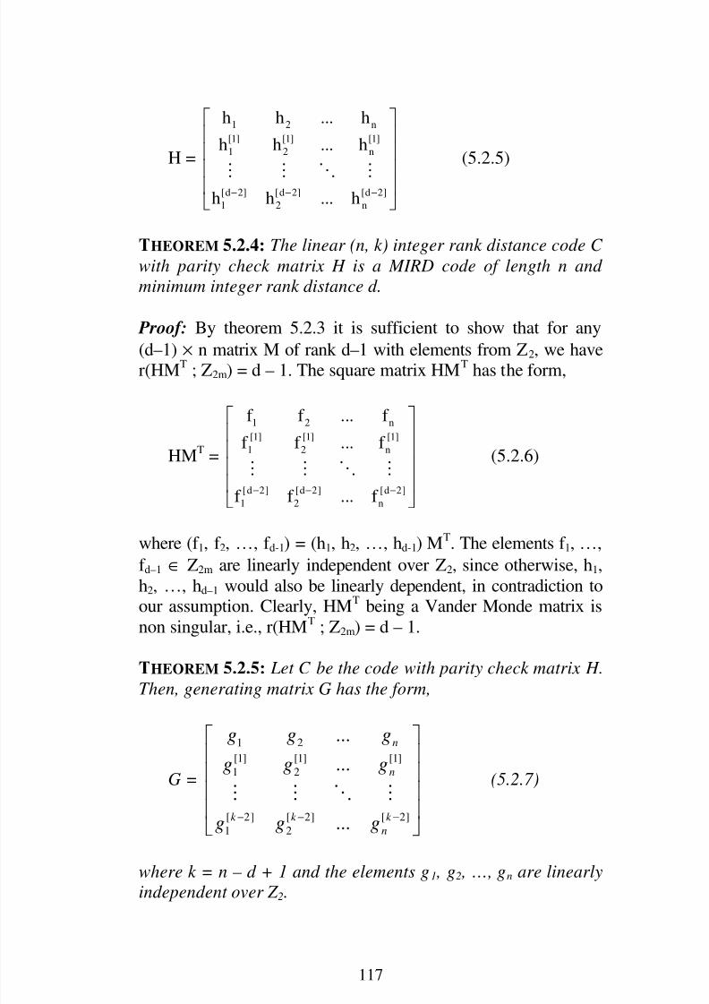
8/2/2019 Erasure Techniques in MRD Codes, by W. B. Vasantha Kandasamy, Florentin Smarandache, R. Sujatha, R. S. Raja …
http://slidepdf.com/reader/full/erasure-techniques-in-mrd-codes-by-w-b-vasantha-kandasamy-florentin-smarandache 118/164
117
H =
1 2 n
[1] [1] [1]
1 2 n
[d 2] [d 2] [d 2]
1 2 n
h h ... h
h h ... h
h h ... h− − −
(5.2.5)
THEOREM 5.2.4: The linear (n, k) integer rank distance code C
with parity check matrix H is a MIRD code of length n and
minimum integer rank distance d.
Proof: By theorem 5.2.3 it is sufficient to show that for any
(d–1) × n matrix M of rank d–1 with elements from Z2, we haver(HM
T; Z2m) = d – 1. The square matrix HM
Thas the form,
HMT
=
1 2 n
[1] [1] [1]
1 2 n
[d 2] [d 2] [d 2]
1 2 n
f f ... f
f f ... f
f f ... f − − −
(5.2.6)
where (f 1, f 2, …, f d-1) = (h1, h2, …, hd-1) MT. The elements f 1, …,
f d–1 ∈ Z2m are linearly independent over Z2, since otherwise, h1,
h2, …, hd–1 would also be linearly dependent, in contradiction toour assumption. Clearly, HM
Tbeing a Vander Monde matrix is
non singular, i.e., r(HMT
; Z2m) = d – 1.
THEOREM 5.2.5: Let C be the code with parity check matrix H.
Then, generating matrix G has the form,
G =
1 2
[1] [1] [1]
1 2
[ 2] [ 2] [ 2]
1 2
...
...
...
n
n
k k k
n
g g g
g g g
g g g− − −
(5.2.7)
where k = n – d + 1 and the elements g1 , g2 , …, gn are linearlyindependent over Z 2.

8/2/2019 Erasure Techniques in MRD Codes, by W. B. Vasantha Kandasamy, Florentin Smarandache, R. Sujatha, R. S. Raja …
http://slidepdf.com/reader/full/erasure-techniques-in-mrd-codes-by-w-b-vasantha-kandasamy-florentin-smarandache 119/164
118
Proof: From theorem 5.2.4 with d = n–1, there exist elements f 1,
f 2, …, f n ∈ Z2m which are linearly independent over Z2 andsatisfy
n[s ]
1 i
i 0
f h=
∑ , s = 0, 1, …, n–2. (5.2.8)
Since f 1, f 2, …, f n are linearly independent over Z2,[ k 1] [ k 1] [ k 1]
1 2 nf ,f ,..., f − + − + − + are also linearly independent over Z2. We
take g1 = [ k 1]
1f − + , g2 = [ k 1]
2f − + , …, gn = [ k 1]
nf − + to be the first row
of the matrix (5.2.7).
As polynomials with coefficients from Z2m play an
important role in the theory of maximum distance separablecodes over Z2m the linearized polynomials play similar role in
the theory of maximum rank distance codes over GF(2N) [29,
32]. In a analogous way we can use linearized polynomial withcoefficients from Z2m to study MIRD codes over Z2m.
A linearized polynomial is one of the form F (z) =n
[1]
1
i 0
f z=
∑ ,
[i] = 2i, where f i ∈ Z2m. We define the sums of the polynomialsas
F(z) + G(z) =n
[1]
1
i 0
f z=
∑ +n
[1]
1
i 0
g z=
∑
= [i ]2m i i
i 0
R (f g )z=
+∑
where R2m (f i + gi) is the least nonnegative integer when f i + gi isdivided by the integer 2m. The multiplication product is the
symbolic product F * G = F (G(z)). This multiplication
operation is non-commutative. The set of all linearizedpolynomials with coefficients from Z2m form a non-
commutative ring with identity element f 0
(z) = z.

8/2/2019 Erasure Techniques in MRD Codes, by W. B. Vasantha Kandasamy, Florentin Smarandache, R. Sujatha, R. S. Raja …
http://slidepdf.com/reader/full/erasure-techniques-in-mrd-codes-by-w-b-vasantha-kandasamy-florentin-smarandache 120/164
119
Generalized Inversionless Euclidean algorithm for division
(whether left or right) of one polynomial by another exists inthis ring. Here we consider right division.
Let F0(z) and F1(z) be two linearlized polynomials with
degF1(z) < degF0(z). Then by generalized Euclidean algorithmwe get a sequential chain of equalities
F0(z) = G1(z) * F1(z) + F2(z), degF2(z) < degF1(z)F1(z) = G2(z) * F2(z) + F3(z), degF3(z) < degF2(z)
(5.2.9)
Fs-1
(z) = Gs(z) * F
s(z) + F
s+1(z), degF
s+1(z) < degF
s(z)
Fs(z) = Gs+1(z) * Fs+1(z)
The last non zero remainder Fs+1(z) in this chain is the right
symbolic LCD of polynomials F0(z) and F1(z). If we introducepolynomials Ui(z), Ai(z), Vi(z) and Bi(z), defined recursively for
i ≥ 1, by
Ui (z) = Ui–1(z) * Gi(z) + Ui–2(z), U0(z) = z, U–1(z) = 0
Ai(z) = Gi(z) * Ai–1(z) + Ai–1(z), A0(z) = z, A–1(z) = 0Vi(z) = Vi–1(z) * Gi(z) + Vi–1(z), V0(z) = z, V–1(z) = z
(5.2.10)
Bi(z) = Bi–1(z) * Gi(z) + Bi–2(z), B0(z) = z, B–1(z) = zthen,
F0(z) = Ui(z) * Fi(z) + Ui–1(z) * Fi+1(z) (5.2.11)F1(z) = Vi(z) * Fi(z) + Vi–1(z) * Fi+1(z).
In addition,
Fi(z) = (–1)i(Bi–1(z) * F0(z) – Ai–1(z) * Fi(z)). (5.2.12)
Consider the factor ring0NR which is the ring of the
linearlized polynomials over Z2m modulo[ ]0N
z – z. Theelements of this factor ring are also linearlized polynomials of
degree ≤ [N0] – 1.

8/2/2019 Erasure Techniques in MRD Codes, by W. B. Vasantha Kandasamy, Florentin Smarandache, R. Sujatha, R. S. Raja …
http://slidepdf.com/reader/full/erasure-techniques-in-mrd-codes-by-w-b-vasantha-kandasamy-florentin-smarandache 121/164
120
Let F(z) =0N 1
[i ]
1
i 0
f z−
=
∑ ∈ 0NR . Raising the polynomial to the
power 2 we get F
[1]
(z) =0
0 0
[N 1][1] [0] [1] [1] [1]
N 1 0 N 2f z f z ... f z
−
− −+ + + whichis equivalent to raising all its coefficients to the power 2 and
then performing a cyclical shift. This operation will be called as
a 2-cyclical shift.
The ideals in0N
R are principal ideals and are generated by
polynomials G(z) that are right divisors of 0[N ]z – z i.e., the
polynomial G(z) is such that 0[N ]z – z = H(z) * G(z). The ideal
{G(z)} is invariant under 2-cyclical shift.
The codes with generator matrix of the form (5.2.7) can be
described in terms of the linearlized polynomials. Assume thatg1, g2, …, gn are specified elements that are linearly independent
over Z2. Then all vectors of the form
g = (F(g1), F(g2), …, F(gn)), where F(z) extends over alllinearlized polynomials of degree less than or equal to [k–1] =
2
k–1
with coefficients from Z2m are codewords.
Code C is called 2-cyclical if a 2-cyclical shift of any
codeword is also a codeword i.e., if (g0, g1, …, gn–1) ∈ C then its
2-cyclic shift [1] [1] [1]
n 1 0 n 2g ,g ,...,g− − ∈ C. This is analogous to the
usual cyclic codes over the integer ring.
Let us consider, for simplicity, codes with length n = No.
Assume that G(z) =r
[i ]
i
i 0
G z=
∑ is a right zero divisor of
0[N ]z – z. Then, its 2-cyclical code consists of all polynomials of
the form c(z) * G(z), where c(z) is an arbitrary linearlized
polynomial of degree ≤ (N0 – r – 1). The dimension of the codeis k = N0 – r. Its generator matrix has the form

8/2/2019 Erasure Techniques in MRD Codes, by W. B. Vasantha Kandasamy, Florentin Smarandache, R. Sujatha, R. S. Raja …
http://slidepdf.com/reader/full/erasure-techniques-in-mrd-codes-by-w-b-vasantha-kandasamy-florentin-smarandache 122/164
121
G =
0 1 r
[1] [1] [1]
0 r 1 r
[k 1] [k 1] [k 1] [k 1]
0 1 2 r
G G ... G 0 0 ... 0
0 G ... G G 0 ... 0
0 0 ... G G G ... G
−
− − − −
(5.2.13)
If 0[N ]z – z = G(z) * H(z), where G(z) is the generator
polynomial then H(z) can be taken as the corresponding check
polynomial.
We note that an element in V is a code vector if and only if the corresponding linearlized polynomial can be divided without
remainder by the generating polynomial G(z).
In otherwords, an element g is a code vector if and only if
the corresponding polynomial g(z) is such that
g(z) * H(z) ≡ 0 mod ( 0[N ]z – z).
If H(z) =k
[i ]
i
i 0
H z=
∑ is a check polynomial, then the check
matrix has the form
H =
0
[1] [k]
k k 1 0
[1] [k] [k 1]
k 1 0
[N 1][r 1] [r ]
k k 1 0
H H ... H 0 0 ... 0
0 H ... H H 0 ... 0
0 0 ... 0 H H ... H
−
−
−−
−
(5.2.14)
=
0 1 k
[1] [1] [1]
0 k 1 k
[r 1] [r 1] [r 1] [r 1]
0 1 2 k
h h ... h 0 0 ... 0
0 h ... h h 0 ... 0
0 0 ... h h h ... h
−
− − − −
where [k 1]
i k iH h−
−= .

8/2/2019 Erasure Techniques in MRD Codes, by W. B. Vasantha Kandasamy, Florentin Smarandache, R. Sujatha, R. S. Raja …
http://slidepdf.com/reader/full/erasure-techniques-in-mrd-codes-by-w-b-vasantha-kandasamy-florentin-smarandache 123/164
122
Now we proceed onto give the coding and decoding
techniques of MIRD codes.
As in the case of cyclic codes over the integer ring,systematic coding can be effected either by means of a check
polynomial or by means of a generating polynomial.
If H(z) =k
[i ]
i
i 0
H z=
∑ is a check polynomial, then each
g(z) =
0N 1[i ]
ii 0 g z
−
=∑ satisfies g(z) * H(z) = 0, which gives
0
0
k [N i j 1]
N i j 1 j
j 0
g H− − +
− − +
=
∑ = 0, i = 0, 1, …, N0 – 1. (5.2.15)
If we assume that0 0N 1 N k
g ,...,g− − are information symbols
then we can determine the check symbols0N k 1 0
g ,...,g− − .
Assume that we are given the generating polynomial
G(z) =0N 1
[i]
i
i 0
G z−
=
∑ . We divide the polynomial
G0(z) = 0 0
0 0
N 1 N k
N 1 N k g z ... g z
− −
− −+ + on the right by G(z) to get
G0(z) = Q(z) * G(z) + R(z), deg. R(z) < [N0 – k] (5.2.16)
The coefficients0N 1
g − for degrees [N0 – i], i = 1, …, N0 of
the remainder are the check symbols.
MIRD codes with check matrix (5.2.5) can be decoded
using an algorithm that is similar to the algorithm for maximum
rank codes over fields [32] with appropriate modifications due
to the presence of zero divisors. Let g = (g1, g2, …, gn) be thecode vector. e = (e1, e2, …, en) be the error vector and y = g + e
be the received vector. We first calculate the syndrome

8/2/2019 Erasure Techniques in MRD Codes, by W. B. Vasantha Kandasamy, Florentin Smarandache, R. Sujatha, R. S. Raja …
http://slidepdf.com/reader/full/erasure-techniques-in-mrd-codes-by-w-b-vasantha-kandasamy-florentin-smarandache 124/164
123
s = (s0, s1, …, sd–2) = yHT = eHT. (5.2.17)
The decoders problem is to determine the error vector e on the
basis of the known syndrome vector s. Assume that the rank norm of the error vector is m. Thus we have
e = EN = (E0, E1, …, Em)N (5.2.18)
where E0, E1, …, Em are linearly independent over Z2 and
N = (Nij) is a m × n matrix of rank m with elements from Z2.Thus (5.2.17) can be written as
s = ENHT = EX (5.2.19)
where the matrix X = NHT has the form,
X =
[1] [d 2]
1 1 1
[1] [d 2]
2 2 2
[1] [d 2]m m m
x x ... x
x x ... x
x x ... x
−
−
−
where xp =n
pj j
j 1
N h=
∑ , p = 1, 2, …, m (5.2.20)
are linearly independent over Z2. (5.2.19) is equivalent to the
system of equations in the unknowns E0, E1, …, Em, x1, x2, …,xm.
m[p ]
i i
i 1
E x=
∑ = sp, p = 1, 2, …, d–2. (5.2.21)
Assuming that the solution of this system has been found,we can determine the matrix N and the error vector e from
(5.2.20) and (5.2.18). For m ≤ (d – 1) / 2 all the solutions lead tothe error vector e. Thus, the decoding problem reduces to the
solution of system (5.2.20) for the smallest possible value of m.
The solution to the system (5.2.21) is unique if and only if all

8/2/2019 Erasure Techniques in MRD Codes, by W. B. Vasantha Kandasamy, Florentin Smarandache, R. Sujatha, R. S. Raja …
http://slidepdf.com/reader/full/erasure-techniques-in-mrd-codes-by-w-b-vasantha-kandasamy-florentin-smarandache 125/164
124
the error magnitudes E0, E1, …, Em are units analogous to the
case of the maximum distance codes over the integer rings [32].
We introduce the polynomial s(z) =d 2 [ j]
j
j 0
s z−
=∑ , corresponding
to the syndrome s. Assume that Λ(z) =m
[p]
p
p 0
z=
Λ∑ , Λm = 1,
denotes a polynomial whose roots are all possible linear
combinations of E0, E1, …, Em with coefficients from Z2. Let
F(z) =m 1
[i ]
i
i 0
Fz−
=
∑ , where Fi =i
[p]
p i p
p 0
s −
=
Λ∑ , i = 0, 1, …, m–1.
We have the equality
F(z) = Λ (z) * s (z) mod z[d–1] (5.2.22)
Indeed,
Λ (z) * s (z) =m
[p ]
p
p 0
(s(z))=
Λ∑
=m d 1
[i] [p]
p j
i 0 p j i
z s+ −
= + −
Λ∑ ∑ .
But for m ≤ i ≤ d – 2, we havem
[p] [p]
p j p i p
p j i p 0
s s −
+ − =
Λ = Λ∑ ∑
=
[p ]m m
[ j p]
p j j
p 0 j 1
E x−
= =
Λ
∑ ∑
= ( )m
[i]
j j
j 1
x E 0=
Λ =∑ ,
since Λ (E j) = 0, j = 1, 2, …, m.

8/2/2019 Erasure Techniques in MRD Codes, by W. B. Vasantha Kandasamy, Florentin Smarandache, R. Sujatha, R. S. Raja …
http://slidepdf.com/reader/full/erasure-techniques-in-mrd-codes-by-w-b-vasantha-kandasamy-florentin-smarandache 126/164
125
If the coefficients of polynomial F(z) are known, then the
coefficients of polynomial Λ (z).
Λ0 = j
j
F
s
Λp =
p 1[i ]
j p i p j i
i 0
[p]
j
F s
s
−
+ − −
=
− Λ∑, p = 1, 2, … (5.2.23)
where for j + p ≥ m we set F j+p = 0.
Now we assume that E0, E1, …, Em as well as the
coefficients of Λ(z), are known. We consider the followingtruncated system in the unknows:
m[p]
j j
j 1
E x=
∑ = sp, p = 1, 2, …, m–1. (5.2.24)
We will solve (5.2.23) using the method of successiveelimination of variables. We set Aij = E j, Q1p = sp; we multiplythe (p+1)-th equation of the system by A11, we extract the root
of degree 2, and we subtract the p-th equation. As a result we
obtain a system that does not contain x1 :
p[p]
1j j
j 1
A x=
∑ = Q1p, p = 0, 1, 2, …, m–2 (5.2.25)
where
A1j = A1j =
[ 1]
1j
11
A
A
−
A11, j = 2, …, m.
Q1p = A1p –
[ 1]
1p 1
11
Q
A
−
+
A11, p = 0, 1, …, m – 2. (5.2.26)

8/2/2019 Erasure Techniques in MRD Codes, by W. B. Vasantha Kandasamy, Florentin Smarandache, R. Sujatha, R. S. Raja …
http://slidepdf.com/reader/full/erasure-techniques-in-mrd-codes-by-w-b-vasantha-kandasamy-florentin-smarandache 127/164
126
Repeating this process m – 1 times, and retaining the first
equations obtained from the systems at each step, we arrive at asystem of linear equations with a upper triangular coefficient
matrix:
m
1j j
j 1
A x=
∑ = Qi0, p = 0, 1, 2, …, m. (5.2.27)
where
A1j = E j, j = 1, 2, …, m
A1j =[ 1]
(i 1) j
(i 1) j
(i 1)(i 1)
0 if j i
AA
A
−
−
−
− −
<
−
A(i–1)(i–1) if j ≥ i; i = 2, 3, …, m
(5.2.28)
Q1p = sp, p = 0, 1 , …, m – 1
Q1j = Q(i–1)p
[ 1]
( 1)( 1)
( 1)( 1)
i p
i i
Q
Q
−
− +
− −
A(i–1)(i–1) p = 0, 1, …, m – i;
i = 2, …, m (5.2.29)
The solution of (5.2.25) can be found by back substitution i.e.,
xm = m0
mm
Q
A
xm–i =
m
(m i)i (m i) j j
j m i 1
(m i)(m i)
Q A x
A
− −
= − +
− −
− ∑, i = 1, 2, …, m – 1. (5.2.30)
We now state the above in the form of a decoding algorithm.

8/2/2019 Erasure Techniques in MRD Codes, by W. B. Vasantha Kandasamy, Florentin Smarandache, R. Sujatha, R. S. Raja …
http://slidepdf.com/reader/full/erasure-techniques-in-mrd-codes-by-w-b-vasantha-kandasamy-florentin-smarandache 128/164
127
Step 1: We calculate the syndrome s = (s0, s1, …, sd–2) and the
corresponding polynomial s (z) =
d 2[ j]
j j 0 s z
−
=∑ .
Step 2: We set F0(z) = z[d–1], F1(z) = s(z) and employ
generalized Euclidean algorithm until we reach a F1+1(z) such
that deg F1(z) ≥ 2(d–1)/2 , deg F1+1(z) < 2(d–1)/2. Then
∆(z) = γ Am(z)
F(z) = γ (–1)m Fm+1(z) (5.2.31)
where, γ is chosen such that the coefficient of Λ m is equal to 1.
Polynomial Λ(z) can be determined either on the basis of the first formula in (5.2.22), if polynomials Ai(z), i = 1, 2, …,
are calculated in parallel in the course of Euclidean algorithm,
or using (5.2.23), which employ the coefficients of the
remainder Fm+1(z) calculated in the course of the algorithm.Then roots E0, E1, …, Em of Λ(z) that are linearly independentover Z2 are determined.
Step 3: Using 5.2.27 to 5.2.30 the known E0, E1, …, Em are usedas a basis for determining x1, x2, …, xm. Representing these
quantities in the form (5.2.20), we can obtain matrix N. Finally,
we calculate the error vector using (5.2.29).
Example 5.2.1: The code with the following parity check matrix
H =1 4 2
1 2 4
has length n = 3 and the designed distance d = 3.
Let y = (3, 2, 1) be the received codeword. Then, the syndrome
is s = (s0, s1) = yHT
= (5, 5). Hence, by modified inversionless
Euclid’s algorithm,

8/2/2019 Erasure Techniques in MRD Codes, by W. B. Vasantha Kandasamy, Florentin Smarandache, R. Sujatha, R. S. Raja …
http://slidepdf.com/reader/full/erasure-techniques-in-mrd-codes-by-w-b-vasantha-kandasamy-florentin-smarandache 129/164
128
Λ(z) = – ( [1]
0s / s1) + z[1] = –5z + z2. The nonzero root of
Λ(z) is 5. Hence, E = 5. From the single equation of the system(5.2.26) we determine
x = (s1 / s0) = 1 = (1 × 1) + (0 × 4) + (0 × 2) = y1 h1 + y2 h2 +
y2 h2) which gives (y1, y2, y3) = (1, 0, 0). The error vector ise = (y1 E, y2E, y3E) = (5, 0, 0)
We have constructed a new class of effective erasure codesover the ring of integers using the rank distance metric. This
class of codes can be suited in different applications like reliable
computer communication protocols, ARQ protocols in satellitescommunications and in amateur radios.

8/2/2019 Erasure Techniques in MRD Codes, by W. B. Vasantha Kandasamy, Florentin Smarandache, R. Sujatha, R. S. Raja …
http://slidepdf.com/reader/full/erasure-techniques-in-mrd-codes-by-w-b-vasantha-kandasamy-florentin-smarandache 130/164
129
Chapter Six
CONCATENATION OF ALGEBRAIC CODES
In this chapter we study concatenation of linear block code with
another linear block code or concatenation of three or more
linear block codes. We describe this in section one. This chapterhas two sections. In section two we describe concatenation of
RD codes with CR-matric. We give the probable ways of building concatenated bicodes, biconcatination of codes andquasi concatenated bicodes.
6.1 Concatenation of Linear Block Codes
The construction and the encoding procedure of the
concatenated codes is described in this section which is as
follows:Let S = ((n1, n2, …, nt), (k 1, …, k t)) be the special supercode
defined over the Galois field Z2 = GF(2) and the inner codes C1
= C1(n1, k 1), C2 = C2(n2, k 2), … and Ct = Ct(nt, k t) be codes withHamming metric defined over the Galois field GF(2).
Suppose m = (x1 | x2 | … | xt) be the message to be encoded
where each xi is a k i tuple of the formi
i i i
1 2 k (a ,a ,...,a ) ;
1 ≤ i ≤ t, thus we get x = (b1 | b2 | … | bt) where bi =
i
i i i
1 2 n(a ,a ,...,a ) ; 1 ≤ i ≤ t wherei
ja ∈ GF(2); 1 ≤ j ≤ ni; 1 ≤ i ≤ t.

8/2/2019 Erasure Techniques in MRD Codes, by W. B. Vasantha Kandasamy, Florentin Smarandache, R. Sujatha, R. S. Raja …
http://slidepdf.com/reader/full/erasure-techniques-in-mrd-codes-by-w-b-vasantha-kandasamy-florentin-smarandache 131/164
130
Thus we have a k 1 + k 2 + … + k t dimensional super vector
space associated with this concatenated code or the super codeis a k 1 + k 2 + … + k t dimensional vector subspace of a
n1 + n2 + … + nt dimensional vector space over Z2. Infact S has1 2 tk k ... k
2+ + +
elements.
We can consider a map;
g : S → (C1 × C2 × … × Ct) = {(x1, x2, …, xt) | xi ∈ Ci,
1 ≤ i ≤ t} given by g ((x1 | … | xt)) = (x1, x2, …, xt) where
xi ∈ Ci; 1 ≤ i ≤ t. This map g is one to one linear transformation
of S to C1 × C2 × … × Ct.
So S ≅ (C1 × C2 × … × Ct) just ‘|’ replaced by ×.
The concatenated code is comprised of the outer code and tnumber of inner codes. The outer code is a super code and the t-
inner codes are the row submatrices of the outer code. That is
the outer code which is the super code has its sub row vectors
from these t inner codes. The t inner codes can be distinct orotherwise. The following is the concatenated coding system.
Thus we see the concatenated code word which is a supercode takes the form of a super row matrix
x =1
1 1 1
1 2 n(x ,x ,..., x2
2 2 2
1 2 nx ,x ,...,x …t
t t t
1 2 nx , x ,..., x ) with j
px ∈
Z2; 1 ≤ j, p ≤ t and the concatenated code
S = {x = 11 1 11 2 n(x ,x ,..., x 2
2 2 21 2 nx ,x ,...,x … tt t t1 2 nx ,x ,...,x |
j
j j j
1 2 nx ,x ,..., x ) ∈ C j = C j (n j, k j); 1 ≤ j ≤ t; j
px ∈ Z2; 1 ≤ j, p ≤ t}.

8/2/2019 Erasure Techniques in MRD Codes, by W. B. Vasantha Kandasamy, Florentin Smarandache, R. Sujatha, R. S. Raja …
http://slidepdf.com/reader/full/erasure-techniques-in-mrd-codes-by-w-b-vasantha-kandasamy-florentin-smarandache 132/164
131
For any two x, y ∈ S we can define dS (x, y) =t
j j j
j 1
d (x , y )=
∑
where x j, y j ∈ C j (n j, k j); 1 ≤ j ≤ t. It is easily verified dS(x, y) =dS(x+y) denotes the super Hamming metric on S over
GF(2) or t-concatenated Hamming metric on S. All properties of
Hamming metric can be derived in case of t-concatenatedHamming metric for the concatenated code S.
Message
Outer encoder
First inner
encodertth
inner encoder
tth
inner decoder
Outer decoder
Decoded
message
…
First inner
decoder…
Channel
…

8/2/2019 Erasure Techniques in MRD Codes, by W. B. Vasantha Kandasamy, Florentin Smarandache, R. Sujatha, R. S. Raja …
http://slidepdf.com/reader/full/erasure-techniques-in-mrd-codes-by-w-b-vasantha-kandasamy-florentin-smarandache 133/164
132
We illustrate this by an example.
Example 6.1.1: Let S = {(x1 | x2 | x3 | x4) | x1 ∈ C (2, 3), x2 ∈
C(5, 2), x3 ∈ C (7, 4) and x4 ∈ C (4, 2)} be a concatenated codewith the codes C1 = C (8, 3), C2 = (5, 2), C3 = C (7, 4) and C4 =
C (4, 2).
We see error detection can be done using the parity check
matrices of C1, C2, C3 and C4.
Error correction can be carried out using coset leader
method [16]. This type of concatenated super codes has the
following advantages.
(i) The rate of transmission is increased.
(ii) This concatenated codes saves time during
transmission as insteaded of sending t-vectors of each nt tuples we send a lengthened code.
(iii) We can retrieve the messages.
Furthert
min min
i 0 ti
d 1 d 1
2 2=
− − ≤
∑ ∑ .
So in a Super code which is the concatenated code usinglinear codes with Hamming metric we can detect and correcterrors, with in the limits of compatibility.
Now we describe another type of concatenated code of alinear codes with Hamming metric.

8/2/2019 Erasure Techniques in MRD Codes, by W. B. Vasantha Kandasamy, Florentin Smarandache, R. Sujatha, R. S. Raja …
http://slidepdf.com/reader/full/erasure-techniques-in-mrd-codes-by-w-b-vasantha-kandasamy-florentin-smarandache 134/164
133
The message x =1
1 1 1
1 2 n(x ,x ,...,x ,2
2 2 2
1 2 nx ,x ,..., x ,
…t
t t t
1 2 nx ,x ,...,x ) is sent to the divider unit which devides them
Source
Divider unit
Message 1 Message t
Super Channel
Encoder
decoder 1 Decoder t
Consolidator
unit
Destination
…
…
Message 1 Message t…
…
…

8/2/2019 Erasure Techniques in MRD Codes, by W. B. Vasantha Kandasamy, Florentin Smarandache, R. Sujatha, R. S. Raja …
http://slidepdf.com/reader/full/erasure-techniques-in-mrd-codes-by-w-b-vasantha-kandasamy-florentin-smarandache 135/164
134
into t messages and the messages are sent to t encoder and they
pass the super channel and reach as t decoders, from the decoderunits reaches the consolidation unit and then the destination.
These codes will be useful when the bulk work is distributed todifferent units and the result is consolidated to get the final
message.
Let C1, C2, …, Ct be t number of linear codes distinct or
otherwise of length n1, n2, …, nt and messages k 1, k 2, …, k t
respectively. We denote by P =1
1 1 1
1 2 n(x ,x ,...,x ,2
2 2 2
1 2 nx ,x ,..., x ,
…t
t t t
1 2 nx ,x ,...,x ) | j
ix ∈ Z2; 1 ≤ j ≤ t and 1 ≤ i ≤ n1, n2, …, nt}.
We say P is concatenated using t inner codes, however P is not asuper code, just a code. By using usual transmission the rate of
transmission is certainly less or equal to the sum of the rates of
transmissions.
The diagram is self explanatory.
We can use error connection technique or erasure correction
technique.
Finally we give yet another type of concatenated linearcodes which we will define in the following. These will also be
known as special blank concatenated codes.
Suppose C1 = C(n, k) code and C2 = C(n, k ′) or C(n–1, k 1)code. Then we form the concatenated code C = C1 C2 = {(x1y1
x2y2 … xn yn) | (x1, x2, …, xn) is in C (n, k) and (y1, y2, …, yn)∈
C(n, k ′)} ((x1 y1 x2 y2 … xn-1 yn-1 xn) where
(x1, …, xn) ∈ C(n, k) and (y1, …, yn–1) ∈ C (n–1, k 1)) will bedefined as the alternate concatenated two code or special blank
concatenated code and the transmission is done using the‘special blank’; however ‘special blanks’ are not erasures.
We will describes how the transmission takes place.

8/2/2019 Erasure Techniques in MRD Codes, by W. B. Vasantha Kandasamy, Florentin Smarandache, R. Sujatha, R. S. Raja …
http://slidepdf.com/reader/full/erasure-techniques-in-mrd-codes-by-w-b-vasantha-kandasamy-florentin-smarandache 136/164
135
Information Source
Converter*
I
(x1–x2–…-xn-)
or (x1-x2-…-xn)
Channel
Reconverter
Receiver
Converter II†
Message
Encoder
(–y1-y2-…-yn-)
or (y1-y2-…-yn-1–)
Converter II †
Message
Encoder
Decoder I
Reconverter I
with special blanks
Decoder II
Reconverter II
with special blanks

8/2/2019 Erasure Techniques in MRD Codes, by W. B. Vasantha Kandasamy, Florentin Smarandache, R. Sujatha, R. S. Raja …
http://slidepdf.com/reader/full/erasure-techniques-in-mrd-codes-by-w-b-vasantha-kandasamy-florentin-smarandache 137/164
136
* converter converts this concatenated code into two codes with
special blanks.† the special blanks are omitted and the message are sent by
converter I and converter II.
This sort of coding will be used in networking where somesecrecy is to be maintained so that processed as two units by
two separate systems and the consolidated result is availed by
the receiver. Likewise we can define m-concatenated codes.Deconverter converts the code words with special blanks into
the concatenated code.
Suppose we have 3 codes say C1 = C(5, 2), C2 = C(6, 3) andC3 = C (5, 3); the 3-concatinated code C = {x1y1z1 x2y2z2 x3y3z3
x4y4z4 x5y5z5 y6) | (x1 x2 … x5) ∈ C1, (y1 y2 y3 y4 y5 y6) ∈
C2 and (z1, z2, …, z5) ∈ C3}.Now this code C of length 16 is sent and converter divides
this into 3 codes of length 16 with special blanks codes writer I,
writer II and writer III, they convert them into messages of
length 5, 6 and 5 respectively and coded and sent via threechannels. We can have m number of codes of lengths n1, n2, …,
nm with message symbols k 1, k 2, …, k m respectively. That is Ci = (ni, k i), 1 ≤ i ≤ m.
Hence C the concatenated m code C1, …, Cm is given by
C = { 1 2 mp p p1 2 m 1 2 m 1 2 m
1 1 1 2 2 2 3 3 3 1 2 mx x ...x x x ...x x x ...x ...x x ...x } where some
pi’s may be zero and some p j’s are n j’s; 1 ≤ i, j ≤ m.Now when any x from C is transmitted x is decomposed
into m units say 1, 2, …, m where the first unit the code words
will be of the form y = ( 11x … 2
1x … 1n1x …), the second unit
y2 = (– 1
2x … – 2
2x … 2n
1x …) and so on. The blanks are special
blanks. From the m-units the m-converters will convert these y1,
y2, …, ym code words into z1 = ( 1n1 2
1 1 1x x ...x ), z2 = ( 2n1 2
2 2 2x x ...x ),
…, zm = ( mn1 2
m m mx x ...x ) by removing the special blanks. Now z1,
z2, …, zm are sent and as in case of usual transmission we getthe received message say as P1, P2, …, Pm then they are passed
through the reconverter where they get the special blanks andthen they pass through the consolidation channel. Then the

8/2/2019 Erasure Techniques in MRD Codes, by W. B. Vasantha Kandasamy, Florentin Smarandache, R. Sujatha, R. S. Raja …
http://slidepdf.com/reader/full/erasure-techniques-in-mrd-codes-by-w-b-vasantha-kandasamy-florentin-smarandache 138/164
137
receiver receives the message which is a concatenated m-linear
code.We just describe the transmission by the following diagram:
Message
Converter*
Writer 1 Writer m
Unit 1 Unit m
Encoder 1 Encoder m
Modulator 1 Modulator m
Channel 1 Channel
message message
(concatenated messageof m codes say of
lengthm
i
i 1
n−
∑ )
…
…
…
…
…
Demodulator 1 Demodulator m
Decoder 1 Decoder m
Receiver 1 Receiver m
…
…
…
8/2/2019 Erasure Techniques in MRD Codes, by W. B. Vasantha Kandasamy, Florentin Smarandache, R. Sujatha, R. S. Raja …
http://slidepdf.com/reader/full/erasure-techniques-in-mrd-codes-by-w-b-vasantha-kandasamy-florentin-smarandache 139/164
138
* Converter converts them into m codes with special blanks.
When the concatenated code of the lengthm
i
i 1
n=
∑ with
concatenated message symbolsm
i
i 1
k =
∑ is sent, then the converter
divides them into m codes of each lengthm
i
i 1
n=
∑ = n1+n2 + … +
nm with special blanks.
Now these are sent to m writers writer 1, writer 2, … writer
m. These writers write the codes by deleating the special blanksspaces.
These units acts as the sender of the message, these
messages are encoded by encoder 1, encoder 2, …, encoder m.From the encoder it passes thro’ the modulator, and from the
modulators to the channels from channels to decoders and from
the decoders to the m receiver if the purpose of the concatenatedcoding is to send the message to m receivers from one sender.
But on the other hand if the purpose is to send to receiverbut each channel or system does a different type of m-jobs and
should reach the single receiver then we have the decoded m-
messages would be sent to m-reversing units and then m of
these reversing units to m-rewriters who include the blanks and
from it reaches a single reconverter and from the reconverter thereceiver receives the message then in that case of extended
diagram would be as follows.

8/2/2019 Erasure Techniques in MRD Codes, by W. B. Vasantha Kandasamy, Florentin Smarandache, R. Sujatha, R. S. Raja …
http://slidepdf.com/reader/full/erasure-techniques-in-mrd-codes-by-w-b-vasantha-kandasamy-florentin-smarandache 140/164
139
D1 decorder Dm decorder
Message
Converter*
Writer 1 Writer m
Unit 1 Unit m
Encoder 1 Encoder m
Modulator 1 Modulator m
Channel
message
…
…
…
…
Channel
Rewriter 1 Rewriter m
Reversing unit mReversing unit 1
Rewriter 1
message
…
…
…
…
Destination

8/2/2019 Erasure Techniques in MRD Codes, by W. B. Vasantha Kandasamy, Florentin Smarandache, R. Sujatha, R. S. Raja …
http://slidepdf.com/reader/full/erasure-techniques-in-mrd-codes-by-w-b-vasantha-kandasamy-florentin-smarandache 141/164
140
Thus it is a 12 step process.
6.2 Concatenation of RD Codes with CR-metric
The concatenated code consists of an outer and an innercode. The outer code is a RD code and the inner code is a binary
code and the outer code is a code over the inner code. The
concatenated code consists of the codewords of the outer code
expressed in terms of the alphabets of the inner code. Thisconcatenated coding system is depicted in the following figure:
From the above figure we see that the encoder of a
concatenated code consists of an outer encoder and an innerencoder corresponding to the outer and inner codes respectively.
Message
Outer Encoder
Inner Encoder
Channel
Inner Decoder
Outer Decoder
Decoder
Message
Super Channel

8/2/2019 Erasure Techniques in MRD Codes, by W. B. Vasantha Kandasamy, Florentin Smarandache, R. Sujatha, R. S. Raja …
http://slidepdf.com/reader/full/erasure-techniques-in-mrd-codes-by-w-b-vasantha-kandasamy-florentin-smarandache 142/164
141
Similarly the decoder of a concatenated code consists of an
outer decoder and an inner decoder corresponding to the outerand inner codes respectively. Here the combination of the inner
encoder, channel and the inner decoder can be thought of asforming a new channel called a super-channel. The super-
channel transmits the codewords of the outer code.
The encoding procedure of concatenated codes is given in
the following section.
Let the outer code A be a linear k a a a 2(n ,k ,d ) RD code
defined over, the Galois field GF(k
2 ) and the inner code B be alinear (nb, k b, db)2 code defined over the Galois field GF (2) of order 2. Throughout this section, we consider the inner code
with Hamming metric. Let m = (a1, a2, …,ak a ) ∈
[GF(k
2 ) ak ] be the message to be encoded, where each ai ∈
GF bk (2 ) . The procedure of concatenation of the outer code A
and the inner code B is given in the following three steps:
Step 1: The message m = (a1, a2, …,ak a ) ∈ GF ( k
2 ) ak ] where
each ai ∈ GF(k
2 ) is encoded with the outer code A into a
codeword. Thus we get a na-tuple a = (a1, a2, …,ana )
Twhere
each ai ∈ GF(k
2 ).
Now a is the codeword of MRD code which is to be
transmitted after applying the following steps:
Step 2: GF(k
2 ) is a k b - dimensional vector space over the
field GF(2). Let g : GF(k
2 ) → [GF(2)k
] be the mapping of
GF(k
2 ) onto [GF(2)k
] such that for each symbol ai ∈
GF(k
2 ), i = 1, 2, …, na is mapped into a k b-dimensional vector
with symbols in GF(2); that is g(ai) = (bli, b2i, …, k ib ) where b ji
∈ GF(2), j = 1, 2, …, k b and i = 1, 2, …, na.

8/2/2019 Erasure Techniques in MRD Codes, by W. B. Vasantha Kandasamy, Florentin Smarandache, R. Sujatha, R. S. Raja …
http://slidepdf.com/reader/full/erasure-techniques-in-mrd-codes-by-w-b-vasantha-kandasamy-florentin-smarandache 143/164
142
Clearly the map g is a one-one linear transformation of the
vector space GF(k
2 ) onto [GF(2)k
] .
Hence, GF(k
2 ) = [GF(2)k
] .
After applying steps 1 and 2 to the message m we denote
the result in the form of a matrix;
a
1
2
n
g(a )
g(a )
...
g(a )
=
b
b
a a b a
11 21 k 1
12 22 k 2
1n 2n k n
b b ... b
b b ... b
... ... ... ...
b b ... b
, (6.2.1)
where bij ∈ GF (2), i = 1, 2, …, k b and j = 1, 2, …, na.
Step 3: Each g (ai) = (b1i, b2i, …, n ib ) is encoded with the inner
code resulting in a codeword from the inner code given by
(b1i, b2i, …, n ib ), where b ji ∈ GF(2), j = 1, 2, …, nb and i = 1, 2,
…, na.
After applying steps 1, 2, and 3 of the encoding procedure
described above to the message m and encoding each row of the
matrix (6.2.1) by using the inner code we get the codeword of the concatenated code represented by the following matrix.
b
b
a a b a
11 21 n 1
12 22 n 2
1n 2n n n
b b ... b
b b ... b
... ... ...
b b ... b
(6.2.2)
where bij ∈ GF(2), i = 1, 2, …, nb and j = 1, 2, …, na.
From here onwards the matrix (6.2.2) will be known as the
Concatenated Code Matrix (CC matrix) and will be denoted by
8/2/2019 Erasure Techniques in MRD Codes, by W. B. Vasantha Kandasamy, Florentin Smarandache, R. Sujatha, R. S. Raja …
http://slidepdf.com/reader/full/erasure-techniques-in-mrd-codes-by-w-b-vasantha-kandasamy-florentin-smarandache 144/164
143
CCM (m), that is, it is the related concatenated code matrix of
the message m.
DEFINITION 6.2.1: The concatenated code obtained byconcatenating the outer RD code, a defined over GF(
k 2 ) and
the inner binary code B is the set of all concatenated code
matrices. Let CCM = {CCM(m) / m ∈ [GF(k
2 ) ak ] } denote the
collection of all (na × nb) CC matrices or equivalently.
CCM = {(bij): bij ∈ GF(2), i = 1, 2, …, na , j = 1, 2, …, nb
and (bij)} is a CC matrix.
DEFINITION 6.2.2: Let CCM be the concatenated code obtained
by concatenating the outer RD code A and the inner binary code
B. For two concatenated code matrices X, Y ∈ CCM define
d c(X, Y) = r (X + Y), where r (X+Y) denotes the rank of the
matrix X + Y over GF (2) obtained by adding the CC matrices X
and Y, using the usual matrix addition modulo 2. That is, if X =
(aij) and Y = (bij) then X + Y = (aij + bij) mod 2.
By the usual properties of the rank of the matrix, for every
X, Y, Z ∈ CCM.
(i) dc (X,Y) ≥ 0(ii) dc (X, Y) = 0 if and only if X = Y,
(iii) dc (X, Y) = dc (Y, X)
(iv) dc (X, Y) ≤ dc (X, Z) + dc (Z, Y).
Thus dc is a metric on the set of all concatenated codematrices on CCM and we define dc as the concatenated rank
metric (CR-metric).
DEFINITION 6.2.3: The set of all concatenated code matrices
(CCM) equipped with the concatenated rank metric (CR-metric)
d c is called the concatenated Rank Metric code (CRM code).

8/2/2019 Erasure Techniques in MRD Codes, by W. B. Vasantha Kandasamy, Florentin Smarandache, R. Sujatha, R. S. Raja …
http://slidepdf.com/reader/full/erasure-techniques-in-mrd-codes-by-w-b-vasantha-kandasamy-florentin-smarandache 145/164
144
Throughout we denote a CRM code by (CCM, dc). It is
clear from the very construction that the CRM code is not a RDcode or a binary code.
DEFINITION 6.2.4: Let (CCM, d c) be a CRM code. The
minimum distance of the concatenated rank metric code (CCM,
d c) is defined as
d = min {r (X+Y) / X, Y ∈ CCM, X ≠ Y}.
For X, Y ∈ CCM we have X + Y ∈ CCM we can restate the
above definition as follows:
DEFINITION 6.2.5: Let (CCM, d c) be a CRM code with d c the
concatenated rank metric. The minimum distance of the
concatenated rank metric code (CCM, d c) is defined as
d = min {r (X) : X ∈ CCM – {0}}.
DEFINITION 6.2.6: Let (CCM, d c) be a CRM code with d c the
concatenated rank metric. Let X ∈ CCM. We say r (X) = 0 if
and ony if X = 0.
DEFINITION 6.2.7: Let (CCM, d c) be a CRM code with d c the
concatenated rank metric. Let m be the transmitted message
with the corresponding CC matrix viz., X = CCM (m). Let Y be
the received matrix. If r (X+Y) = 0, that is, X+Y = 0 which
implies X = Y, then Y is the correct message since addition of X
and Y is under addition modulo 2.
If r (X+Y) > s, s > 0, then Y has an error of rank s.
A relation between the minimum distance of theconcatenated rank metric code and the minimum distance of the
outer RD code is given by the following theorem.
THEOREM 6.2.1: Let the outer code A be a linear k a a a 2(n ,k ,d )
RD code defined over GF(
k
2 ) and the inner code B be abinary linear (nb , k b , d b)2 code defined over GF(2). Let (CCM,
d c) be the concatenated rank metric code with the CR-metric d c

8/2/2019 Erasure Techniques in MRD Codes, by W. B. Vasantha Kandasamy, Florentin Smarandache, R. Sujatha, R. S. Raja …
http://slidepdf.com/reader/full/erasure-techniques-in-mrd-codes-by-w-b-vasantha-kandasamy-florentin-smarandache 146/164
145
obtained by using the outer code A and the inner code B. Then
the minimum distance of the concatenated rank metric code
(CCM, d c) is d a : d a is just the minimum distance of the outer RD
code.
Proof : Let the outer RD code A be a k a a a 2(n ,k ,d ) code with
minimum distance da and let the inner code B be a binary linear(nb, k b, db)2 code defined over GF(2). Let (CCM, dc) be the
concatenated rank metric code obtained by using the outer code
A and the inner code B. Let the message m = (a1, a2, …,ak a ) ∈
[GF(k
2 )k
] where each ai ∈ GF(k
2 ) be encoded with the outer
code A into a codeword a = (a1, a2, …,ana )
T ∈ A. Since the
minimum distance of the outer RD code is da, so r(a) ≥ da. Thisimplies atleast da columns of the matrix a
Tare linearly
independent over GF(2). Without loss of generality let us
assume that the first da columns of the matrix aT
are linearly
independent over GF(2). That is, a1, a2, …,ada are linearly
independent over GF(2). By the method of concatenating the
codes A and B given earlier and after applying the mapping gwe get the matrix
B =
b
b
a a b a
a a b a
11 21 k 1
12 22 k 2
1d 2d k d
1n 2n k n
b b ... b
b b ... b
... ... ... ...
b b ... b
... ... ... ...
b b ... b
where bij ∈ GF(2), i = 1, 2, …, k b and j = 1, 2, …, na.
Since r(a) ≥ da, we get r(b) ≥ da. We have, after applying theinner encoder to the matrix B, let the concatenated code matrix
corresponding to the message m be CCM(m) = b1, that is,

8/2/2019 Erasure Techniques in MRD Codes, by W. B. Vasantha Kandasamy, Florentin Smarandache, R. Sujatha, R. S. Raja …
http://slidepdf.com/reader/full/erasure-techniques-in-mrd-codes-by-w-b-vasantha-kandasamy-florentin-smarandache 147/164
146
b1 =
b
b
a a b a
a a b a
11 21 n 1
12 22 n 2
1d 2d n d
1n 2n nfc n
b b ... b
b b ... b
... ... ... ...
b b ... b
... ... ... ...
b b ... b
where bij ∈ GF (2), i = 1, 2, …, nb and j = 1, 2, …, na.
Then, r(b1) ≥ da since the addition of parity bits by the inner
code B to the matrix b does not change the rank of the matrix b.Hence the minimum distance of the concatenated rank metriccode of da.
The above theorem is illustrated by the following example.
Example 6.2.1: Let the outer code A be a (2, 1, 1) RD code with
minimum distance 1 defined over GF(22) = {0, 1, α, α
2} where
α is the root of the primitive polynomial x2
+ x + 1 of GF(22
).Let the generator matrix of the outer code A be G = (1 0) where
0, 1 ∈ GF(22). Let the inner code B be a binary (4, 2, 3) code
with minimum distance 3 be defined over GF(2) having the
parity check matrix
H =1 0 1 0
1 1 0 1
.
The mapping g : GF(22) → [GF(2)]
2is the mapping given
by the primitive polynomial of GF(22), defined as 0 → 00, 1 →
01, α →10, α2 →11.

8/2/2019 Erasure Techniques in MRD Codes, by W. B. Vasantha Kandasamy, Florentin Smarandache, R. Sujatha, R. S. Raja …
http://slidepdf.com/reader/full/erasure-techniques-in-mrd-codes-by-w-b-vasantha-kandasamy-florentin-smarandache 148/164
147
The concatenated rank metric code
CCM =
0 0 0 0 0 1 0 1
, ,0 0 0 0 0 0 0 0
1 0 1 1 1 1 1 0,
0 0 0 0 0 0 0 0
.
The CCM has minimum distance d = 1, (since rank of reach of the CC matrices in CCM is either zero or one).
In general, in the case of concatenated codes with Hammingmatrix the true minimum distance of the code cannot be
obtained but only a lower bound can be obtained. Whereas for
the CRM code constructed by us the minimum distance
calculated in the above theorem is the true minimum distanceand not a lower bound. We prove this in the following corollary.
Corollary 6.2.1: Let the outer code A be a linear k a a a 2(n ,k ,d ) RD code with minimum distance da defined over GF (
k 2 ) and
the inner code B be a binary linear (nb, k b, db)2 code with
minimum distance db defined GF (2). Let (CCM, dc) be the
CRM code obtained by using the codes A and B. The minimumdistance of the CRM code is the true minimum distance and it is
just the minimum distance of the outer code.
Proof: Let the outer code A be a linear k a a a 2(n ,k ,d ) RD codewith minimum distance da defined over GF(
k 2 ) and the inner
code B be a binary linear (nb, k b, db)2 code defined over GF(2).
Let(CCM, dc) be the concatenated rank metric code obtained by
using the outer code A and the inner code B. From theorem6.2.1 we know that the minimum distance of the concatenated
rank metric code (CCM, dc) is da. Hence the minimum distance
of the concatenated rank metric code is the true minimum
distance and not a lower bound for the minimum distance.

8/2/2019 Erasure Techniques in MRD Codes, by W. B. Vasantha Kandasamy, Florentin Smarandache, R. Sujatha, R. S. Raja …
http://slidepdf.com/reader/full/erasure-techniques-in-mrd-codes-by-w-b-vasantha-kandasamy-florentin-smarandache 149/164
148
It is interesting to note that, in the case of (CCM, dc) code or
CRM codes if we want to have a desired minimum distance wecan without hesitation take the outer RD code with the desired
minimum distance and use any convenient binary inner code,for the minimum distance is independent of he choice of the
inner code. Thus this concatenation technique helps one toconstruct any CRM code of desired minimum distance which is
not enjoyed by any other class of codes.
THEOREM 6.2.2: (Error detection theorem for CRM codes) Let
(CCM, d c) be the concatenated rank metric code with CR-metric
d c obtained by using the codes A and B where the outer code A
is a linear k ba a a 2( n ,k ,d ) RD code defined over GF( bk
2 ) and the
inner code B is a binary linear (nb , k b , d b)2 code defined over
GF(2). Let X be the transmitted CC matrix and Y be the
received matrix. If r(Y) < d a then an error has occurred in the
matrix Y during transmission.
Proof : Let m be the message transmitted. Let X be the
associated concatenated code matrix of m, that is X = CCM(m).Let Y be the received concatenated code matrix which contains
errors occurred during transmission. Suppose r(Y) < da. From
corollary 6.2.1 the minimum distance of the concatenated rank
metric code is the true minimum distance and hence r(X) ≥ da
for every X ∈ CCM. So, r(Y) < da indicates that an error hasoccurred during transmission.
It is very important to note that from the above theorem we
can just by computing the rank of the received matrix, we canimmediately conclude that an error has occurred duringtransmission.
We give the decoding procedure for CRM codes.
Our decoding procedure for CRM codes is nothing but to
obtain a decoding method for the received concatenated codematrix which is done by first decoding with the inner code and
then decoding with the outer code. The reason for doing so is
due to the systematic construction of CRM codes explained

8/2/2019 Erasure Techniques in MRD Codes, by W. B. Vasantha Kandasamy, Florentin Smarandache, R. Sujatha, R. S. Raja …
http://slidepdf.com/reader/full/erasure-techniques-in-mrd-codes-by-w-b-vasantha-kandasamy-florentin-smarandache 150/164
149
earlier. We know by the very construction of the CRM codes
that the received concatenated code matrix has its entries fromthe alphabets of the inner code. Hence the received
concatenated code matrix is first decoded by using the innercode and then it is decoded with the decoding algorithm of the
outer code. Hence the decoder of a concatenated code consistsof an inner decoder and an outer decoder. Now we explain the
decoding procedure for concatenated rank metric codes (CCM,
dc) with CR-matrix dc.
Let Y be the received message. Clearly Y is the matrix
given by
Y =
b
b
a a b a
11 21 n 1
12 22 n 2
1n 2n n n
y y ... y
y y ... y
... ... ...
y y ... y
(6.2.3)
where yij ∈ GF (2), i = 1, 2, …, nb and j = 1, 2, …, na.
We describe the decoding procedure of a received
concatenated code matrix Y in the following three steps.
Step 1: For each i = 1, 2, …, nb decode (y1i, y2i, …, n iy ) using
the inner code decoder and obtain a k b - tuple (y1i, y2i, …, k iy )
where b ji ∈ GF (2), j = 1, 2, …, nb and obtain the matrix.
y =
b
b
a a b a
11 21 k 1
12 22 k 2
1n 2n k n
y y ... y
y y ... y
... ... ...
y y ... y
where yij ∈ GF(2), I = 1, 2, …, k b and j = 1, 2, …, na. Here whendecoding with the inner code the number of columns in the
received concatenated matrix Y is reduced and the number of
row remains unaltered.

8/2/2019 Erasure Techniques in MRD Codes, by W. B. Vasantha Kandasamy, Florentin Smarandache, R. Sujatha, R. S. Raja …
http://slidepdf.com/reader/full/erasure-techniques-in-mrd-codes-by-w-b-vasantha-kandasamy-florentin-smarandache 151/164
150
Step 2: Applying the mapping g-1: [GF(2)
k ] → GF(
k 2 ) on
each row of the matrix y we get zi ∈ GF(k
2 ). Hence
corresponding to the matrix y we obtain a na tuple
(z1, z2, …,anz ) ∈ [GF( k
2 ) an] .
Step 3: Now decode the na-tuple
(z1, z2, …,anz ) ∈ [GF(
k 2 ) an
] using the outer decoder. Thus the
transmitted message corresponding to the received concatenated
code matrix is given by
(z1, z2, …,ak z ) ∈ [GF(
k 2 ) ak
] which gives only the message
symbols.The following examples illustrates the decoding procedure
described above.
Example 6.2.2: Let the outer code A be a (2, 1,1) RD code
defiend over GF(22) = {0, 1, α, α
2} where α is the root of the
primitive polynomial x2
+ 2 + 1 of GF(22). Let the generator
matrix of the outer code A be G = (1 0) where 0, 1 ∈ GF(22).
Let the inner code B be a binary (4,2,3) code defined overGF(2) having the parity check matrix
H =1 0 1 0
1 1 0 1
.
The mapping g : GF(22) → [GF(2)]
2is the mapping given
by the primitive polynomial of GF(22), defined as 0 → 00, 1 →
01, α →10, α2 →11.
The concatenated rank metric code
CCM =0 0 0 0 0 1 0 1
, ,0 0 0 0 0 0 0 0
1 0 1 1 1 1 1 0,0 0 0 0 0 0 0 0
.

8/2/2019 Erasure Techniques in MRD Codes, by W. B. Vasantha Kandasamy, Florentin Smarandache, R. Sujatha, R. S. Raja …
http://slidepdf.com/reader/full/erasure-techniques-in-mrd-codes-by-w-b-vasantha-kandasamy-florentin-smarandache 152/164
151
Suppose the matrix Y =1 1 1 0
1 0 0 0
is received. The
received matrix Y is decoded using the decoding procedure of
CRM codes described above.
By step 1, we first use the inner decoder to decode the
received matrix Y. The inner decoder decodes (1 1 1 0) to (1 1)
and (1 0 0 0) to ( 0 0) to obtain the matrix y =1 1
0 0
.
Then by step 2, on applying the map
g–1
: [GF(2)]2 → GF(2
2) to each row of matrix y, we get y2
=2
0
α
. By step 3, the outer decodes this column vector y2 to α2
the transmitted message symbol (since in this example the RD
code has only one message symbol).
Now from these concatenated MRD codes we can definebiconcatenated MRD codes or concatenated MRD bicodes, C =
C1 ∪ C2 where each Ci is a concatenated CRM codes. We canalso extend this to n-concatenated CRM codes or concatenated
n-CRM codes as C = C1 ∪ C2 ∪ … ∪ Cn where each Ci is a
CRM code; 1 ≤ i ≤ n. This form of n-codes will help in thesimultaneous processing using n-units which will be timesaving.
We can also define quasi n-concatenated CRM codes, when
some t of them are concatenated CRM codes and the rest areMRD codes. Further the n-concatenated special super codes; C
= C1 ∪ C2 ∪ … ∪ Cn if each Ci is a special super code; i = 1, 2,…, n. If n = 2 we get the biconcatenated special super code.
We can also have biconcatenated CRM code with a specialsuper codes defined as mixed biconcatenated code. That is C =
C1 ∪ C2 where C1 is a super special code and C2 is a CRM code.We can extend this to mixed n-concatenated codes where t of

8/2/2019 Erasure Techniques in MRD Codes, by W. B. Vasantha Kandasamy, Florentin Smarandache, R. Sujatha, R. S. Raja …
http://slidepdf.com/reader/full/erasure-techniques-in-mrd-codes-by-w-b-vasantha-kandasamy-florentin-smarandache 153/164
152
them are super special codes (t < n) and rest are just CRM
codes. We can also have the notion of quasi mixed n-concatenated codes where t1 of them are CRM codes, t2 of them
are just MRD codes, t3 of them special super codes and the restof them are just linear codes. Thus we can have quasi mixed n-
concatenated codes. These codes will help when bulk messagesare sent and this will save time and economy.

8/2/2019 Erasure Techniques in MRD Codes, by W. B. Vasantha Kandasamy, Florentin Smarandache, R. Sujatha, R. S. Raja …
http://slidepdf.com/reader/full/erasure-techniques-in-mrd-codes-by-w-b-vasantha-kandasamy-florentin-smarandache 154/164
153
FURTHER R EADINGS
1. Berlekamp, E.R., Algebraic coding theory, McGraw-Hill,New York, 1968.
2. Birkhoff, G., and Maclane, S., A Brief Survey of Modern
Algebra, 2nd
ed, New york: The Macmillan Company, 1965.
3. Blake, I.F., Codes over certain rings, Information Control,
20, 396-404, 1972.
4. Blake, I.F., Codes over integer residue rings, Information
Control, 29, 295-300, 1975.
5. Calderbank, A.R. and N.J.A. Slaone, Modular and p-adic
cyclic codes, Designs, Codes and Cryptography, 6, 21-35,
1995.
6. Forney, G.D., Burst Correcting codes for the classic bursty
channel, IEEE Trans. Comm. Tech., COM-19, 772-781,1971.
7. Forney, G.D., Concatenated codes, MIT Press, Cambridge,1966.
8. Forney, G.D., On decoding BCH codes, IEEE Trans. Inf.
Thy., IT-11, 549-557, 1965.
9. Gabidulin, E.M., Theory of codes with maximum rank
distance, Problems of Information Transmission, 21, 1-12,1985.

8/2/2019 Erasure Techniques in MRD Codes, by W. B. Vasantha Kandasamy, Florentin Smarandache, R. Sujatha, R. S. Raja …
http://slidepdf.com/reader/full/erasure-techniques-in-mrd-codes-by-w-b-vasantha-kandasamy-florentin-smarandache 155/164
154
10. Golay, M.J.E., Notes on Digital Coding, Proc., of the IRE
37, 657-666, 1949.
11. Hamming, R.W., Error detecting and error correcting
codes, Bewll Syst. Tech. Jl., 29, 147-160, 1950.
12. Hill, R., A first course in coding theory, Clarendon, Oxford,
1986.
13. Interando, I.C., Palazzo, R. and M. Elia, On the decoding of
Reed-Solomon and BCH codes over integer residue rings,
IEEE Trans. On information Theory, 43, 1013-1021, 1997.
14. Jungnickel, D., Finite Fields, Structure and arithmetic,
Bibliographisher Institut, Mannheim, 1993.
15. Lempel, A., Matrix Factorization over F 2 and trace-
orthogonal basis of
tmin min
i 0 ti
d 1 d 1
2 2=
− − ≤
∑ ∑ , SIAM
Journal on Computations, 4, 175-186, 1975.
16. Lidl, R. and G. Pilz, Applied abstract algebra, Springer-
verlag, New York, 1984.
17. Luigi Rizzo, Effective erasure codes for reliable computer
communication protocols, Computer Communication
Review, 27, 24-36, 1997.
18. Mac Williams, F.J. and N.J.A. Sloane, The theory of error
correcting codes, North Holland Publishing Company,
1977.
19. Massey, J.L., Linear Codes with complementary duals,
Discrete Mathematics, 106 and 107, 337-342, 1992.
20. Michelson, A.M., and A.H. Leveque, Error-control
techniques for digital communication, John Wiley & Sons,New York, 1985.
21. Peterson W.W. Encoding error correction Procedures for
the Bose-Chaudhuri codes, IRE Trans Inf Thy 6 459-470,1960.
22. Peterson, W.W. and E.J. Weldon, Error correcting codes,M I T Press, Cambridge, 1972.

8/2/2019 Erasure Techniques in MRD Codes, by W. B. Vasantha Kandasamy, Florentin Smarandache, R. Sujatha, R. S. Raja …
http://slidepdf.com/reader/full/erasure-techniques-in-mrd-codes-by-w-b-vasantha-kandasamy-florentin-smarandache 156/164
155
23. Priti Shankar, On BCH codes over arbitrary integer rings,
IEEE Trans on Inform Theory, 25, 480-2, 1979.
24. Raja Durai, R.S., and Vasantha, W.B., Some results on T-
Direct codes, Asia-Europe Workshop on information
theory, Kamogawa, Japan, June 25-28, 2003.
25. Raja Durai, R.S., On linear codes with Rank metric:
Construction, Properties and Applications, Ph.D.
Dissertation, Guide Dr. W.B. Vasantha Kandasamy,
Department of Mathematics, Indian Institute of Technology,Chennai, May 2004.
26. Reed, I.S., and G. Solomon, Polynomial codes over certain finite fields, SIAM Jl. Appl. Maths, 8, 300-304, 1960.
27. Rimoldi, B, Coding for the Guassian multiple access
channel, An algebraic approach, Proceedings of
International Symposium on Information Theory, Austin,
TX, 1993.
28. Shannon, C.E. A mathematical theory of communication,
Bell Syst. Tech., j. 27, 379-426 and 623-656, 1948.
29. Sujatha, R., Construction of concatenation and erasure
techniques for the class of MRD codes and their
applications, Ph.D. Dissertation, Guide: Dr. W.B. Vasantha
Kandasamy, Department of Mathematics, Indian Institute of Technology, Chennai, June 1998.
30. Suresh Babu, N. Studies of rank distance codes, Ph.D.
Thesis, Department of Mathematics, Indian Institute of
Technology, Chennai, 1995.31. Tommy Pedersen, Performance aspects of concatenated
codes, Likeoping studies in Science and Technology,
Dissertations, No. 245, 1992.
32. Vasantha, W.B. and R. Sujatha, Effective erasure codes for
reliable computer communication protocols using codes
over arbitrary integer rings, Prog. of Maths, Vol 32, 187-
207, 1998.

8/2/2019 Erasure Techniques in MRD Codes, by W. B. Vasantha Kandasamy, Florentin Smarandache, R. Sujatha, R. S. Raja …
http://slidepdf.com/reader/full/erasure-techniques-in-mrd-codes-by-w-b-vasantha-kandasamy-florentin-smarandache 157/164
156
33. Wekerly, J.F., Detection of unidirectional multiple errors
using low-cost arithmetic codes, IEEE Trans. Comput., C-24, 210-212, 1975.
34. Zimmermann, K.H., The weight distribution of
indecomposable cyclic codes over 2-groups, Journal of
Combinatorial Theory (A), 60, 85-103, 1992.

8/2/2019 Erasure Techniques in MRD Codes, by W. B. Vasantha Kandasamy, Florentin Smarandache, R. Sujatha, R. S. Raja …
http://slidepdf.com/reader/full/erasure-techniques-in-mrd-codes-by-w-b-vasantha-kandasamy-florentin-smarandache 158/164
157
INDEX
2
2-user F-adder channel, 106-8
A
Abelian group, 7-9
Algebraic linear codes, 29-32ARQ system, 83
B
Binary symmetric channel, 43-5
Binary symmetric erasure channel, 44-6
Blank spaces, 44-6
C
Canonical generator matrix, 35-7Code word, 29-32
Commutative ring, 11-12
Concatenated bicodes, 129-Concatenation of Linear Block codes, 129-32
Coset leader method, 38-40
Coset leader, 38-9CRM code, 142-9

8/2/2019 Erasure Techniques in MRD Codes, by W. B. Vasantha Kandasamy, Florentin Smarandache, R. Sujatha, R. S. Raja …
http://slidepdf.com/reader/full/erasure-techniques-in-mrd-codes-by-w-b-vasantha-kandasamy-florentin-smarandache 159/164
158
CR-metric, 140-9
Cyclic code, 40-4
E
Erasure technique, 41-5Erasures, 43-5
F
Factor group, 10-11
Field, 16-7
G
Group code, 31-3Group, 7-9
I
Integer rank distance code, 112-5Integer rank distance code, 113-9Integer rank distance space, 113-5
Irreducible polynomial, 19-20
L
LCD codes, 101-5
Left ideal, 13-4Linear submodule, 113-5
M
Maximal cyclic codes, 40-3
Maximal ideal, 20-3
Minimal ideal, 20-3MIRD codes, 111-4
MRD codes with complementary duals, 103-5MRD codes, 49-53

8/2/2019 Erasure Techniques in MRD Codes, by W. B. Vasantha Kandasamy, Florentin Smarandache, R. Sujatha, R. S. Raja …
http://slidepdf.com/reader/full/erasure-techniques-in-mrd-codes-by-w-b-vasantha-kandasamy-florentin-smarandache 160/164
159
N
Noiseless 2-user F-adder channel, 106-8Noisy 2-user F-adder channel, 107-8
Normal subgroup, 9-11
P
Parity check code, 34-5
Parity check matrix of a linear code, 31-3
Polynomial ring, 18-9Prime field, 17-8
Q
q-Cyclic MRD codes, 91-4
q-Cyclic RD codes, 83-6
Quasi concatenated bicodes, 129-Quotient ring, 15-6
R
Rank distance code, 46-9
Rank distance space, 46-53
Rank metric, 46-53Rank norm, 46-53
Reducible polynomial, 19-20
Repetition code, 33-5Right coset, 10-11
Right ideal, 13-4
S
Shortened q-cyclic RD-codes, 89-92
special blank concatenated codes, 134-9Special blanks, 46-8, 133-6
Subfield, 17-8Subgroup, 8-10

8/2/2019 Erasure Techniques in MRD Codes, by W. B. Vasantha Kandasamy, Florentin Smarandache, R. Sujatha, R. S. Raja …
http://slidepdf.com/reader/full/erasure-techniques-in-mrd-codes-by-w-b-vasantha-kandasamy-florentin-smarandache 161/164
160
Subring, 12-3
Super code, 129-135
T
t-concatenated Hamming metric, 129-135Transmission rate, 31-3
V
Vander monde Matrix, 116-8
Vector space, 25-6Vector subspace, 25-6

8/2/2019 Erasure Techniques in MRD Codes, by W. B. Vasantha Kandasamy, Florentin Smarandache, R. Sujatha, R. S. Raja …
http://slidepdf.com/reader/full/erasure-techniques-in-mrd-codes-by-w-b-vasantha-kandasamy-florentin-smarandache 162/164
161
ABOUT THE AUTHORS
Dr.W.B.Vasantha Kandasamy is an Associate Professor in the
Department of Mathematics, Indian Institute of TechnologyMadras, Chennai. In the past decade she has guided 13 Ph.D.scholars in the different fields of non-associative algebras,
algebraic coding theory, transportation theory, fuzzy groups, and
applications of fuzzy theory of the problems faced in chemicalindustries and cement industries. She has to her credit 646
research papers. She has guided over 68 M.Sc. and M.Tech.
projects. She has worked in collaboration projects with the Indian
Space Research Organization and with the Tamil Nadu State AIDS
Control Society. She is presently working on a research project
funded by the Board of Research in Nuclear Sciences,Government of India. This is her 66
thbook.
On India's 60th Independence Day, Dr.Vasantha was
conferred the Kalpana Chawla Award for Courage and Daring
Enterprise by the State Government of Tamil Nadu in recognitionof her sustained fight for social justice in the Indian Institute of
Technology (IIT) Madras and for her contribution to mathematics.
The award, instituted in the memory of Indian-American
astronaut Kalpana Chawla who died aboard Space ShuttleColumbia, carried a cash prize of five lakh rupees (the highest
prize-money for any Indian award) and a gold medal.
She can be contacted at [email protected]
Web Site: http://mat.iitm.ac.in/home/wbv/public_html/ or http://www.vasantha.in
Dr. Florentin Smarandache is a Professor of Mathematics atthe University of New Mexico in USA. He published over 75 books
and 200 articles and notes in mathematics, physics, philosophy,
psychology, rebus, literature. In mathematics his research is innumber theory, non-Euclidean geometry, synthetic geometry,
algebraic structures, statistics, neutrosophic logic and set(generalizations of fuzzy logic and set respectively), neutrosophic
probability (generalization of classical and imprecise probability).Also, small contributions to nuclear and particle physics,
information fusion, neutrosophy (a generalization of dialectics),
law of sensations and stimuli, etc. He got the 2010 Telesio-Galilei
Academy of Science Gold Medal, Adjunct Professor (equivalent toDoctor Honoris Causa) of Beijing Jiaotong University in 2011, and
2011 Romanian Academy Award for Technical Science (the
highest in the country). Dr. W. B. Vasantha Kandasamy and Dr.
Florentin Smarandache got the 2011 New Mexico Book Award forAlgebraic Structures. He can be contacted at [email protected]

8/2/2019 Erasure Techniques in MRD Codes, by W. B. Vasantha Kandasamy, Florentin Smarandache, R. Sujatha, R. S. Raja …
http://slidepdf.com/reader/full/erasure-techniques-in-mrd-codes-by-w-b-vasantha-kandasamy-florentin-smarandache 163/164
162
Dr. R.Sujatha has obtained her doctorate degree on Algebraic
Coding Theory from Indian Institute of Technology under the
guidance of Dr. W.B.Vasantha, Department of mathematics, IIT
(madras) Chennai – 36. She is presently working in SSN college
of engineering. She has 14 years of teaching and researchexperience. She has published over 35 research articles and has
authored two books.She can be contacted at [email protected]
Dr. R.S.Raja Durai is an Assistant Professor of Jaypee University
of Information Technology, has obtained his doctorate from theIndian Institute of Technology, Chennai – 36, under the guidance
of Dr.W.B.Vasantha Kandasamy. He has published over 10
research papers and is currently guiding Ph.D students.

8/2/2019 Erasure Techniques in MRD Codes, by W. B. Vasantha Kandasamy, Florentin Smarandache, R. Sujatha, R. S. Raja …
http://slidepdf.com/reader/full/erasure-techniques-in-mrd-codes-by-w-b-vasantha-kandasamy-florentin-smarandache 164/164