erdc/gsl tn-16-1 'predicting soil strength in terms … · clays (ch). the atterburg limits in...

Approved for public release; distribution is unlimited.

PURPOSE: A study was conducted of parameters used to adequately describe soil strength for trafficability as related to changes in moisture. Modeling the weather conditions in combination with the terrain will create dynamically changing soil conditions. Off-road predictions of mobility, the detection of buried ordnance, and expedient horizontal construction require a firm understanding of these temporal and spatial changes in the heterogeneous soil system. To validate and verify the soil parameters used to drive a model, rapid and repeatable methods of measuring the soil strength and related physical properties are desired. These testing methods, in turn, drive the selection of appropriate soil parameters. Physical properties of the soil (moisture, porosity, density, chemistry) are not as dependent on the measuring device as mechanical soil properties. Furthermore, the measured physical soil properties do not always provide a direct correlation to the mechanical parameters. Moreover, the temporal and spatial variability of the soil often require the quantification of additional states (i.e., correlations to water table depth). This paper reviews the field tests used to describe the lumped parameters in a soil for trafficability predictions. The parameters of specific interest, in this paper, are those used in the NATO Reference Mobility Model Version 2 (NRMMII) sub-models describing temporal and spatial changes of the soil as a function of weather conditions. Current measurement methods to these approaches are described.

INTRODUCTION: Soil systems are a combination of water, solids, and gases. Modeling soil-strength variations requires input parameters to adequately describe the migration of water in the soil. While the temporal component is correlated to water migration, the spatial component is defined by the variability of the soil type and changes in topography (i.e. elevation, vegetation). Together, the spatial and temporal variations in the physical properties of the soil describe vehicle mobility/trafficability in regions of interest.

The mechanical properties of the soils are determined by introducing stress and strain rates on the soil. From this standpoint, field-measured soil strength is an ambiguous measurement related to the device used and the strain rate and pressure exerted. Error rates, defined by the coefficient of variation, are as high as 40 percent for measurements of cohesion, 12 percent for angle of friction, and 30 percent on the compression index (Harr 1987). Over the years, the types of devices for soil strength measurement related to mobility have been numerous (Bekker 1969). Dynamic types of measurements including the Clegg Hammer and Drop Hammer are used for dry/hard soils. For soft soils, engineers consider the use of cone penetrometers, beveameters, cylindrical plungers, or vane shear devices. Certain modifications of the cone penetrometer, such as a cone mounted on a shear graph, have been developed to measure normal and shear stress of the soil at the same time (Thangavadivelu et al. 1994). Single-wheel tire and track testers have been used to define shear strength and sinkage of the soil (Upadhyaya 1997). The researchers

ERDC/GSL TN-16-1 March 2016

Predicting Soil Strength in Terms of Cone Index and California Bearing Ratio

for Trafficability By George L. Mason and E. Alex Baylot


2

in each case relate soil strength as a function of the physical properties of the soil. Correlations are made to soil type, density, and moisture content. The strategy is to use direct measurements of soil strength to understand and optimize engineering design of vehicles, while using the correlation to physical properties to forecast mobility over a large area with varying time scales.

Soil Strength Related to Moisture Content. To predict seasonal forecasts of mobility, water budget models were employed with relationships between mobility/traction and soil moisture (Kennedy et al. 1988). Although the U.S. Army Engineer Research and Development Center (ERDC) field studies seldom produced smooth curves, laboratory studies conducted in the 1960s relating soil moisture and soil strength as cone index showed a relatively smooth curvilinear relationship and are described by Equation 1 (Knight 1961). These relationships were determined for the Unified Soil Classification System (USCS).

g[ a b ln ( m )]CI e (1)

where:

CI = soil strength in terms of Cone Index1 mg = percent moisture content as expressed as weight of soil a, b = coefficients specified for each USCS type

Moisture is often related as a function of dry unit weight (γd) of the soil as opposed to percent volume of water, because density plays an important part in the buoyancy of the vehicle. Equation 2 is the definition of moisture content by weight.

γγ

w w wg

s d s

V Wm

V W (2)

where:

Vw = volume of water (ft3) VS = volume of solid (constant) (ft3) γw = unit weight of water (lb/ft3) γd = dry unit weight of soil (lb/ft3) wW = weight of water sW = weight of soil

To capture the effect of vehicle traffic and/or compaction, additional formulation was developed called the Rating Cone Index (RCI). To obtain this index, a soil sample is subjected to 100 blows with a 2.5 lb drop hammer falling 12 in. per blow. The inverse of the ratio of measured CI before and after the process is termed Remolding Index (RI). The product of the CI and RI is the RCI.

1 Cone Index is the resistance (lbs) to penetration developed by a cone and is equal to the vertical force applied to the sleeve divided by its surface area. The cone has a 30⁰ apex angle and a 0.5in2 base area.


3

Furthermore, additional research conducted by the ERDC produced a variation of Equation 1 whereby RCI is defined similarly as CI and is expressed as Equation 3 (Knight 1961). The coefficients are different for the soil types when RI is not equal to one. Currently, models such as the Soil Moisture Soil Strength Prediction Model (SMSP) use the generalized relationships (Equations 1 and 3), with the coefficients defined in Table 1 for USCS classes (Sullivan et al. 1997). Table 1 reports average values with variances reported by Sullivan et al. (1997); Clapp and Hornberger (1978); Sellers et al. (1986).

Table 1. Soil Coefficients for Defining Soil Strength from USCS and Moisture.

USCS Soil Type

Empirical Constant β

Residual Moisture

Saturated Moisture (%) m*

Dry Density (lb/ft3) γd CI coeff a CI coeff b

RCI coeff a′

RCI coeff b′

SW 1.852 1.60 34.70 93.6 3.987 0.8150 3.97 0.815 SP 1.852 1.60 34.70 93.6 3.987 0.8150 3.987 0.815 SM 2.375 2.60 40.80 93.7 8.749 -1.1949 12.542 -2.955 SC 2.667 5.60 41.90 97.4 9.056 -1.3566 12.542 -2.955 SM-SC 2.597 4.80 41.80 100.5 9.056 -1.3566 12.542 -2.955 CL 4.505 3.60 46.90 86.8 10.998 -1.848 15.506 -3.530 ML 4.202 2.60 53.70 73.7 10.255 -1.565 11.936 -2.407 CL-ML 4.292 2.60 46.80 83.7 9.454 -1.385 14.236 -3.137 CH 5.208 7.10 47.50 85.5 13.641† -2.417† 13.686 -2.705 MH 4.878 3.80 54.70 66.2 12.321 -2.044 23.641 -5.191 OL 3.876 3.00 62.70 77.4 10.977 -1.754 17.399 -3.584 OH 4.237 4.10 89.20 52.5 13.046 -2.172 12.189 -1.942 GM 3.247 4.10 43.80 GC 4.065 3.40 45.20 * Gravimetric † Correction to references [6], [7], [8]

g[ a b ln ( m )]RCI e (3)

where:

RCI = soil strength in terms of Rating Cone Index a′, b′ = coefficients specified for each USCS

Additionally, early research conducted by the ERDC described RCI as a function of percent fines and constants as coefficients given in Equation 4 (Anderson 1983). One can see the variation to Equation 1 (McDaniel and Smith 1971). Collins and Molthan suggested the lower and upper limits of this relationship were bounded by a multiple parameter formula that included liquid limit, plastic limit, percent fines, percent clays, and the amount of drainage, as defined by a wetness index term (Collins 1971; Molthan 1967).


4

2 123 0 008 0 693

4 6050 0149 0 002

g. . (%clay ) . ln( m )

[ . ]. . (%clay )RCI e (4)

where:

RCI = soil strength in terms of Rating Cone Index clay = clay as defined through hydrometer testing, generally an average diameter of

.0015 nm or less

Figure 1 illustrates the relationship between soil moisture and soil strength for highly plastic clays (CH). The Atterburg limits in Figure 1 are defined by the shrinkage, plastic, and liquid limit ranges. The ranges of liquid, plastic, and shrinkage limits are derived from the USCS classification charts for a CH soil type. Soil strength as defined by RCI is decreasing with moisture content. The probability of immobilization is defined at an RCI below 40 in Figure 1 (Meyer 1966). As indicated in Figure 1, soil moisture increases with decreasing soil strength. As the soil moisture approaches the liquid limit, the probability of immobilization increases. Figure 1 is based on the 0 to 6-in. average soil strength as measured by a cone penetrometer. The relationship between strain, pressure, and the liquid limit of clay is defined by Terzaghi (Terzaghi and Peck 1948). Equation 4 was plotted on Figure 1 against Equation 3. Equation 3 appeared to provide a better depiction of strength versus moisture. Equation 3 is bound with dashed lines indicating the standard deviation reported by the field data.

Figure 1. Relationship between moisture and strength.

Physical properties of the soil including density, volume of water, liquid limit, plastic limit, percent fines and percent clay appear to correlate with soil strength. The migration of water through the soil is correlated to the tension and permeability of the soil (Caron et al. 1992; Clapp and Hornberger 1978; Sellers et al. 1986). To understand the relationship between


5

extremes in moisture and strength within an area of interest on mobility, a short series of NRMMII model runs were conducted. Figure 2 displays three different scenarios conducted with the NRMMII for a small island in the Philippines (McDaniel and Smith 1971).

Figure 2. Migration of Water.

Other factors besides soil strength such as slope, vegetation, and obstacles control vehicle speed. During poor weather conditions, however, soil strength will be a key factor. The Wet-Slippery conditions are considered when the top layer has reached a point of saturation. Tests conducted by Moore (1989) suggested a reduction in traction of greater than 50 percent for off-road travel during periods of rain greater than 0.25 in. within a 15-min period. Moore’s tests were conducted in areas of high humidity and low wind speed, so significant evaporation was not observed. Surface soil strengths did not show correlations with the rain and traction of the vehicle. However, moisture contents of the near surface suggested saturation levels.

Temporal changes in surface moisture are affected by precipitation, evaporation, runoff, and migration of water through the soil. Modeling moisture content of a soil in a layered system can be conducted using a finite difference water budget model illustrated in Figure 2 (Sellers et al. 1986).

Figure 2 shows how flow Q through the soil layer ij is modeled. In general, saturation of layer Qi due to rainfall is modeled by Equation 5. For the study introduced by Janett, a 50 RCI or less for the top 1 cm was used to define a slippery condition for fine-grain soils (Janett et al. 2000).

Evaporation Precipitation

(+)Qi

Runoff

Root Structure

(+)Qij(-)Qij

(+)Qj(-)Qj


6

1 2

1 1

1

11 11

2

11 1 1

1

1

,

i ,i i .i

i ,i out

w t , w t ,

i iw t , w t .i

i i

iQw t ,n

i

dV V Q E R td

d dV V Q O td d

dV Q td

(5)

where:

Q = Flow through a layer (LT-1) E = Evaporation at the near surface (LT-1) R = Runoff of the surface Layer (L)

Often, simulations introduce weather through seasonal changes or real time movement of weather fronts (Ahlvin and Haley 1992; Janett et al. 2000; Mason 2000). Modeling moisture flow through the soil requires information regarding tortuosity, connectivity, and pore size of the soil. Solutes moving through the soil take a curved path while migrating through the soil pores. The complexity of this path is defined as the tortuosity of the soil. From these parameters permeability and tension of the soil are determined as a function of moisture content. Measurement of these parameters requires advanced equipment such as a synchrotron (Gantzer et al. 2003). Often permeability and tension are inferred from the soil type (Moore 1989). Porosity, which is inversely proportional to the void ratio, is related directly to dry density and defines moisture content at saturation. Often, as found in testing by Moore, the surface is compacted with a low void ratio (Moore 1989). The result is inundation with water, causing saturation to occur early. Surface soil strength as measured with a cone penetrometer does not change appreciably, and the amount of moisture required for saturation is reduced. It is, however, the reduction in shear strength of the soil that reduces traction, and saturation levels can be monitored and modeled to support predictions of slippery conditions.

The rate at which the tire or track shears the soil, often measured by slip, will affect the performance of the vehicle. Meier and Baladi (1988) introduced the shear modulus of the soil as a method to convert the static cone penetration tests to cohesion and shear strength of the soil.

Relationship between Rating Cone Index and California Bearing Ratio. The trafficability of a soil is dependent on having sufficient bearing capacity to support the vehicle and having sufficient traction capacity to develop the resistance between the traction element and the soil to overcome the rolling resistance and provide thrust (WES 1948). If the bearing capacity is low, a vehicle’s traction elements will sink and, thus, increase rolling resistance. As described in the previous section, CI is the resistance (lbs) to penetration developed by a cone and is equal to the vertical force applied to the cone tip divided by its projected surface area.

There are various cone sizes; the cone penetrometer used by the military in soft soil conditions has a 30° apex angle and a 0.5-in2 base area. As previously mentioned, RCI is calculated from the product of a CI measurement and the RI. The California Bearing Ratio (CBR) is the ratio


7

(expressed as a percentage) of the load required to cause the same penetration into the sample as it would a standard, compacted crushed-stone sample. The loading device measures the load required to cause 0.1 in. penetration of a cylindrical plunger measuring 3 square in. of end area.

The CBR has been a key measure for the design of flexible pavements for both roads and airfields since its development in the 1940s. It was devised by Jim Porter ( 1 9 5 0 ) of the California Division of Highways. Porter developed curves showing the relationship between bearing ratios and pavement thicknesses for wheel loads up to 12,000 pounds and correlates these curves with field performance. With the help of Thomas A. Middlebrooks of the U.S. Army Corps of Engineers, the curves were extrapolated to heavier loads. The CBR method is widely accepted as an empirical approach for designing unsurfaced or surfaced pavements with tradeoffs in CBR and layer thickness. Recent research at the ERDC has re-defined the CBR equation to be based on stress distribution for a particular stress concentration factor (Barker and Gonzalez 2006).

Although CBR is primarily used for design of pavements, runways, etc. it is instructive to note the relationship between RCI (or CI) and CBR when predicting the soil strength of in-situ conditions for either trafficability or expedient construction. Field tests have shown a linear or fairly linear relationship between the two measures of soil strength. A study in 1981 by Waterways Experiment Station (WES) showed that for non-plastic soils, CI measured to be about 70 times greater than CBR (Willoughby and May 1981). Earlier studies at WES showed that for clay soils of high plasticity, CI measured to be about 20 times greater than CBR and 50 times greater for less plastic silts and clays (Willoughby and May 1981).

Research conducted since 2004 has strived for the compilation of WES and ERDC field data relevant to soil strength measurements into a single data base dating back to 1948. This research has supported the Opportune Landing Site and Joint Rapid Airfield Construction projects. Parameters include, but are not limited to: geospatial coordinates, landform, gravimetric moisture content, soil type (USCS), specific gravity, dry density, CI, RCI, and CBR. Data records total more than 14,000 in all.

Of those 14,000 records, 209 have corresponding values for gravimetric moisture content (m), RCI, and CBR. Table 2 presents the empirical regression relationships derived from the field data for USCS soil types CH, MH, CL, and ML. Additionally, groupings of soil types are presented. The significance of the groupings is that the NRMMII internally groups the USCS soil types prior to modeling the trafficability/mobility of a vehicle. Thus, the parametric values are the same for particular USCS soil types found in a grouping. Those groupings are: (a) SC, GC, (b) CH, MH, OH, (c) ML, ML-CL, CL, OL, (d) SM, SM-SC, GM, GM-GC, (e) SP, SW, GP, GW, (f) Pt, and (g) rock. Additionally, the available soil types used in this study were combined to represent a “fine-grain” category referred to as “All.” The empirical equations defining the relationship are given in Equations 6 and 7.

Equation 6 bears resemblance to Equations 1, 3, and 4 in that it is natural logarithmic based, but is a simpler form. This is not an endorsement of one form over another. Additional research would be required for such a matter. Equation 7 is a power-based form. This form allows for near-linearity or linearity as the data tends to indicate. This property was anticipated, as CBR and RCI are both measures of soil strength.


8

Table 2. Empirical Regression Data for CBR versus m and RCI.

USCS Soil Type

Number Samples

mg RCI Practical Range of CBR Values **

a b R2 a b R2 Minimum Maximum

CL 30 129.1 -0.199 0.574 0.0173 1.0 0.908 5 15 ML 6 4169.2 -0.2673 0.985 0.0162 1.0 0.954 5 15 CL and ML 36 74.674 -0.1635 0.512 0.0172 1.0 0.914 5 15 CH 96* 11.934 -0.0429 0.326 0.0228 1.027 0.919 3 5 MH 76 58.743 -0.0795 0.688 0.0153 1.0 0.737 4 8 CH and MH 172* 23.816 -0.0602 0.509 0.0184 1.019 0.874 3 8 All 208* 12.86 -0.0498 0.371 0.0180 1.0 0.738 3 15 * Note: an outlier data point was omitted ** Fang 1991 [29]

g[ b m ]CBR a e (6)

where:

CBR = soil strength in terms of California Bearing Ratio a, b = coefficients specified for each USCS soil type or grouping

and

b'CBR a' RCI (7)

where:

a′, b′ = coefficients specified for each USCS soil type or grouping

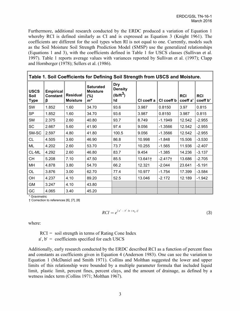
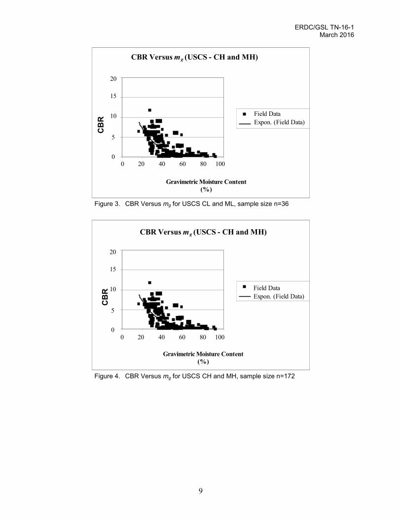
As indicated by the values of the coefficients of fit (R2), the regression fit for CBR versus mg are not particularly good. This is not unlike previous research where the spread of the data is broad [13]. Although the value of R2 for the soil type ML is high, the sample size was only 6; thus, the regression should be used with caution. As might be expected, one can see the similarities in the RCI versus mg curve represented in Figure 1 and the CBR versus mg curves found in Figures 3 through 5. For illustration purposes, only the graphs of soil groupings were presented in this paper. The grouping of “All” was evaluated to provide how lumping all of the soil types together might prove out.

The data for soil types; CL, ML, and the grouping CL and ML provided a linear fit with a coefficient-of-fit to be greater than or equal to 0.91. The data for soil type MH provided a linear fit of 0.737. The data for the remaining soil type CH and the grouping CH and MH were better fitted with a non-linear curve with R2 coefficients of 0.919 and 0.874, respectively. For CBR versus RCI, the grouping of “All” was evaluated only as a linear function to express the overall relationship as a ratio. As with CBR versus mg, only the groupings relationships were provided as Figures (6, 7, and 8).


9

Figure 3. CBR Versus mg for USCS CL and ML, sample size n=36

Figure 4. CBR Versus mg for USCS CH and MH, sample size n=172

Field Data Expon. (Field Data)

Gravimetric Moisture Content (%)

0 20 40 60 80 100

20

15

10

5 0

CB

R

CBR Versus m g (USCS - CH and MH)


Gravimetric Moisture Content (%)

0 20 40 60 80 100

20

15

10

5 0

CB

R

CBR Versus m g (USCS - CH and MH)


10

Figure 5. CBR Versus m for all available soil types, sample size =208

Figure 6. CBR Versus RCI for USCS CL and ML, sample size n=36.

CBR Versus m g (All)


GMC

0 20 40 60 80 100

20

15

10

5

0

CB

R

CBR versus RCI (USCS – CL and ML)

Field Data Linear (Field Data)

RCI

0 20 40 60 80 100

20

15

10

5

0

CB

R


11

Figure 7. CBR Versus RCI for USCS CH and MH, sample size n=172.

Figure 8. CBR Versus RCI for all available soil types, sample size n=208.

CONCLUSIONS: This review of the relationship between physical properties of the soil and mechanical strength shows that the properties vary as a function of moisture and certain site-specific characteristics. These site-specific characteristics may include swelling potential, tortuosity, connectivity, and pore size. The results of the included analysis of recent research shows a similar non-linear relationship between RCI-mg and CBR-mg and a fairly linear relationship between RCI and CBR. Thus, the inference of CBR from RCI is a reasonable estimation. In general, the ratio of values between CBR to RCI is 1:56 for the fine-grain grouping of CL, ML, CH, and MH. However, individual soil types or the selected groupings of (a) CL and ML and (b) CH and MH are better estimators as the practical range of CBR values are more defining (Fang

CBR Versus RCI (USCS – CH and MH)

Field Data Power (Field Data)

RCI

0 200 400 600 800 1000

14

12

10

8

6

4 2

0

CB

R

CBR Versus RCI (All)

Field Data Linear (Field Data)

RCI

0 200 400 600 800 1000

20

15

10

5

0

CB

R


12

1991). Additional research on predicting CBR values from a broader set of parameters is found in Semen (2006).

ACKNOWLEDGEMENTS: The studies described and the resulting data presented herein, unless otherwise noted, were obtained from research conducted under the Joint Rapid Airfield Construction Program of the U.S. Army Corps of Engineers and the Opportune Landing Site Program of the U.S. Air Force. Permission was granted by the Director, Geotechnical and Structures Laboratory, to publish this information.

REFERENCES

Ahlvin, R. B., and P. W. Haley. 1992. NATO reference mobility model, Edition II, NRMM II user's guide. TR GL-92-19. Vicksburg, MS: U.S. Army Engineer Waterways Experiment Station.

Anderson, M. G. 1983. On the applicability of soil water finite difference models to operational trafficability models. Journal of Terramechanics 20(¾):139-152.

Barker, W., and C. Gonzalez. 2006. Reformation of the CBR equation. ERDC/GSL TR (draft). Vicksburg, MS: U.S. Army Engineer Research and Development Center.

Bekker, M. G. 1969. Introduction to terrain-vehicle systems. Ann Arbor, MI: The University of Michigan Press.

Caron, J., B. D. Kay, J. A. Stone, and R. G. Kachanoski. 1992. Modeling temporal changes in structural stability of a clay loam soil. Soil Science 56:1597-1604.

Clapp, R. B., and G. M. Hornberger. 1978. Empirical equations for some soil hydraulic properties. Water Resource Research 14:601-604.

Collins, J. G. 1971. Forecasting trafficability of soils: Relations of strength to other properties of fine-grained soils and sands with fines, report 10. TM No. 3-331, July 1971. Vicksburg, MS: U.S. Army Engineer Waterways Experiment Station.

Fang, Hsai-Yang. 1991. Foundation engineering handbook, 2nd Edition. New York, NY: Van Nostrand Reinhold.

Gantzer, C. J., S. S. Assouline, and S. S. Anderson. 2003. Synchrotron CMT-measured soil physical properties influenced by soil compaction. Research proposal US-3393-03R submitted to the Binational Agricultural Research and Development Fund.

Green, J. G., R. A. Jones, and M. Gallagher. 1997. Mobility assessment of Marine Corps wheeled and tracked vehicles using the Stochastic Mobility Model. Technical Report GL-97-19. Bethesda, MD: Department of the Navy, Naval Surface Warfare Center.

Harr, M. 1987. Reliability-based design in civil engineering. New York, NY: McGraw-Hill Book Company.

Janett, A. C., J. S. Adelson, D. D. Miller, and R. A. Reynolds. 2000. The FOM for atmosphere, ocean, space, and dynamic terrain – environment federation. Simulation Interoperability Workshop Paper 00F-SIW-092.

Kennedy, J. G., E. S. Rush, G. W. Turnage, and P. A. Morris. 1988. Updated soil moisture-strength prediction (SMSP) methodology. Technical Report GL-88-13. Vicksburg, MS: U.S. Army Engineer Waterways Experiment Station.

Knight, S. J. 1961. Some factors affecting moisture content-density-cone index relations. Miscellaneous Paper No. 4-457, Nov 1961. Vicksburg, MS: U.S. Army Engineer Waterways Experiment Station.

Mason, G. L. 2000. Short-term operational forecasts of trafficability (SOFT). Simulation Interoperability Workshop Paper 00S-SIW-066.

Mason, G. L, R. Ahlvin, and J. Green. 2001. Short-term operational forecasts of trafficability. ERDC/GSL TR-01-22. Vicksburg, MS: U.S. Army Engineer Research and Development Center.

McDaniel, A.R., and M. H. Smith. 1971. Trafficability predictions in tropical soils. MP 4-355, August 1971. Vicksburg, MS: U.S. Army Engineer Waterways Experiment Station.


13

Meier, R. W., and G. Y. Baladi. 1988. Cone-index-based estimates of soil strength: Theory and user’s guide for computer code CIBESS. Technical Report SL-88-11. Vicksburg, MS: U.S. Army Engineer Waterways Experiment Station.

Meyer, M. P. 1966. Comparison of engineering properties of selected temperate and tropical surface soils. TR 3-732, June 1966. Vicksburg, MS: U.S. Army Engineer Waterways Experiment Station.

Molthan, H. D. 1967. Influence of soil variability on soil moisture and soil strength predictions. Appendix E in Report of Conference on Soil Trafficability Prediction. Vicksburg, MS: U.S. Army Engineer Waterways Experiment Station.

Moore, D. W. 1989. The influence of soil surface conditions on the traction of wheeled and tracked military vehicles. TR GL-89-6. Washington, DC: Department of the Army U.S. Army Corps of Engineers.

Porter, O. James. 1950. Development of the original method for highway design. In Transactions, American Society of Civil Engineers, 461-67. New York: American Society of Civil Engineers.

Sellers, P. J., Y. Mintz, Y. C. Sud, and A. Dalcher. 1986. A simple biosphere model (SIB) for use within general circulation models. Journal Atmospheric Sciences 43:505-531.

Semen, P. M. 2006. A generalized approach to soil strength prediction with machine learning methods. ERDC/CRREL TR-06-15. Vicksburg, MS: U.S. Army Engineer Research and Development Center.

Sullivan, P. M., N. A. Renfroe, M. R. Albert, G. G. Koening, L. Peck, L., and K. O’Neill. 1997. Soil moisture strength prediction model version II (SMSP II). TR GL-97-15. Vicksburg, MS: U.S. Army Engineer Waterways Experiment Station.

Terzaghi, K., and Ralph B. Peck. 1948. Soil mechanics in engineering practice. New York: John Wiley & Sons Inc.

Thangavadivelu, S., R. Taylor, S. Clark, and J. Slocombe. 1994. Measuring soil properties to predict tractive performance of an agricultural drive tire. Journal of Terramechanics 31(4):215-227.

Upadhyaya, S. K. 1997. Semi-empirical traction prediction equations based on relevant soil parameters. Journal of Terramechanics 34(3):141-154.

U.S. Army Engineer Waterways Experiment Station. 1948. Trafficability of soils, laboratory tests to determine effects of moisture content and density variations. TM 3-240/1, March 1948. Vicksburg, MS: WES.

Willoughby, William E., and Carl R. May. 1981. Boeing/WES mobility tests of transporter tires on Terex 33-15 (draft). Vicksburg, MS: U.S. Army Engineer Waterways Experiment Station.

NOTE: The contents of this technical note are not to be used for advertising, publication, or promotional purposes. Citation of trade names does not constitute an official endorsement or approval of the use of such products.

erdc/gsl tn-16-1 'predicting soil strength in terms … · clays (ch). the atterburg limits in...

Documents