espacioinvestiga.orgespacioinvestiga.org/wp-content/uploads/2016/03/erems2_25092015.pdf · erems2:...
TRANSCRIPT

EREMS2: an Estimated Rational ExpectationModel for Simulation and historical
decomposition of the Spanish economy∗
J.E. Boscáa, R.Doménecha,b, J. Ferria, R. Méndez-Marcanob,c and J.Rubio-Ramírezd
a University of Valenciab BBVA Research
c CESMa-Universidad Simón Bolívard Duke University
February, 2015
Abstract
In this paper we develop and estimate a new bayesian DSGE model for the Spanish economy that hasbeen designed to evaluate different structural reforms. The small open economy model incorporatesa banking sector, consumers and entrepreneurs that accumulate debt, a rich fiscal structure andmonopolistic competition in products and labor markets, for a country in a currency union, withno independent monetary policy. The model can be used to evaluate ex-ante and ex-post policiesand structural reforms and to decompose the evolution of macroeconomic aggregates according todifferent shocks.
Keywords: collateral constraints, banks, bank capital, fiscal policy, sticky interest rates.JEL Classification: E30, E32, E43, E51, E52, E62.
1. Introduction
{TO BE COMPLETED}
∗ The authors thank the excellent research assistance of A. Buesa. The financial support of CICYT grantECO2011-29050 is gratefully acknowledged. J. E. Boscá and J. Ferri also acknowledge the financial supportthrough the collaboration agreement between the Fundación Rafael del Pino, BBVA Research, Ministry of Fi-nance and Ministry of Economy and Competitiveness. All remaining errors are our own responsibility.

CAN STRUCTURAL REFORMS HELP SPAIN? 2
2. Model descriptionThe structure of the economy is as follows. We consider an open economy in which thehome country (Spain) is relatively small to rest of the world, whose equilibrium is inthe limit taken as exogenous (see, for example, Monacelli, 2003, or Galí and Monacelli,2005). The home economy belongs to a monetary union with a central bank controllingthe nominal interest rate. The home economy trades with the rest of the world (in our casethe monetary union) consumption and investment goods as well as international nominalbonds. There are three types of households: patient, impatient, and hand-to-mouth. Thepatient (impatient) households consume, save (borrow), supply labor, and accumulatehousing services. The hand-to-mouth households consume and have access neither todeposits nor to loans. Households delegate their labor decisions to labor unions whooperate in monopolistically competitive markets. There are entrepreneurs whose mainrole is to purchase capital and rent it to intermediate good producers. In addition, entre-preneurs consume and borrow. Entrepreneurs buy capital from capital good producerswho produce capital goods using final goods as inputs. Intermediate good producershire labor from patient, impatient, and hand-to-mouth households, and rent capital fromentrepreneurs in order to produce intermediate goods that are then sold to good retailers.Retailers buy intermediate goods and relabel them at no cost in order to sell them toconsumers and capital producers in a monopolistically competitive market. The bankingsector of the economy operates as follows. Banks form holding units each composed bythree branches: a wholesale bank, a loan-retailing bank, and a deposit-retailing bank.Patient households deposit their savings on deposit-retailing banks. Impatient house-holds and entrepreneurs take loans on loan-retailing banks. Deposit-retailing and loan-retailing banks operates in monopolistically competitive markets. The wholesale bankmanages the capital position of the holding and intermediates funds between the deposit-retailing banks and the loan-retailing banks while counting on the monetary authority tofully-allotting their funding requirements at the policy rate. The source of monopolisticcompetition lies in the presence of differentiated types of labor, retail goods, deposits andloans, but for avoiding the complexities from introducing them explicitly in householdpreferences and good production technology, it is postulated the existence of intermediary"packers" who buy the different types of commodities and bundle or pack them and sellthe homogeneous bundle to households and firms correspondingly.
Although implicitly there is at the union level a monetary authority that fixes theone-period nominal interest rate using a Taylor rule and supplys full-allotment refinancingto wholase banks, following Schmitt-Grohé and Uribe (2003), to ensure stationarity ofequilibrium we assume that banks pay a risk-premium that increases with the country’snet foreign asset position. Thus, we close the model by assuming that the foreign borro-

CAN STRUCTURAL REFORMS HELP SPAIN? 3
wing interest rate is equal to an exogenous interest rate multiplied by a risk premium.Finally, there is a fiscal authority that consumes, invests, borrows or lends, sets lump-sumtaxes, and taxes consumption, housing services, labor earnings, capital earnings, bondholdings, and deposits.
2.1 Patient HouseholdsThere is a continuum of patient households in the economy indexed by j, with mass γp,whose utility depends on consumption, cp
j,t; housing services, hpj,t; and hours worked, `p
j,tand has the following form:
E0
+∞
∑t=0
βtp
(1− acp)εzt log(cp
j,t − acpcpt−1) + ahpεh
t log(hpj,t)−
a`p`p1+φ
j,t
1+ φ
,
where cpt denotes average patient housholds consumption, i.e,
cpt = γ−1
p
(∫ γp
0cp
j,tdj)
;
εzt is a shock to consumption preferences with law motion
log εzt = (1− ρz)log εz
ss + ρzlog εzt−1 + σzez
t where ezt ∼ N (0, 1) ;
and εht is a shock to housing preferences with law of motion
log εht = (1− ρh)log εh
ss + ρhlog εht−1 + σheh
t where eht ∼ N (0, 1).
The jth patient household is subject to the following budget constraint (expressedin terms of final goods):
(1+ τct )c
pj,t + (1+ τh
t )qht ∆hp
j,t + dj,pt + τ
f dt ∆dp
j,t =
(1− τwt )w
pj,t`
pj,t +
[1+(1−τd
t )rdt−1
πt
]dp
j,t−1 +JRt
γp+ (1−ωb)
Jbt−1γp− Tup
tγp− Tg
tγp+γi+γe
.
where πt =Pt
Pt−1is gross inflation with Pt denoting the price level of final goods and
the variables τct , τh
t , τdt and τ
f dt denote taxes on consumption, accumulation of housing
services, interest income from deposits, and deposit transactions, respectively. The flowof expenses, expressed in terms of final goods, are consumption (plus consumption taxes),

CAN STRUCTURAL REFORMS HELP SPAIN? 4
(1+ τct )c
pj,t; accumulation of housing services (plus housing services taxes), (1+ τh
t )qht ∆hp
j,t;
current deposits, dpj,t, and taxes on the variation in the stock of deposits, τ
f dt ∆dp
j,t. The
sources of income are labor income (minus wage income taxes), (1− τwt )w
pj,t`
pj,t; deposits
gross return from the previous period (minus interes income taxes),[
1+(1−τdt )r
dt−1
πt
]dp
j,t−1;
dividends from the retail firms, JRt
γp; dividends from the banking sector, (1− ωb)
Jbt−1γp
, net
of lump-sum fees paid to the unions, Tupt
γp; and lump-sum taxes paid to the government,
Tgt
γp+γi+γe.
Households have access to a Arrow-Debreu securities. We do not write the wholeset of possible Arrow-Debreu securities in the budget constraint to save on notation. Sincetheir net supply is zero, they are not traded in equilibrium. However, households couldtrade and price any of these securities.
The representative patient household chooses cpj,t, dp
j,t, hpj,t (decision on wp
j,t and lpj,t is
delegated on a "labor union" whose decision is described below) for t = 0, 1, 2, ...,+∞ inorder to maximize utility subject to budget constraint. The lagrangian of this maximizationproblem is
E0
+∞
∑t=0
βtp
(1− acp)εzt log(cp
j,t − acpcpt−1) + ahpεz
t log(hpj,t)−
a`p`p1+φ
j,t
1+ φ
−λpj,t
{(1+ τc
t )cpj,t + (1+ τh
t )qht ∆hp
j,t + (1+ τf dt )∆dp
j,t−
(1− τwt )w
pj,t`
pj,t −
[1+ (1− τd
t )rdt−1
πt
]dp
j,t−1 −JRt
γp− (1−ωb)
Jbt−1γp
+Tup
tγp
+Tg
tγp + γi + γe
}],
and the corresponding first order conditions are
λpj,t(1+ τc)−
(1− acp)εzt
cpj,t − acpcp
t−1= 0
ahpεht
hpj,t− λ
pj,t(1+ τh)qh
t + βpEt
{λ
pj,t+1(1+ τh)qh
t+1
}= 0
λpj,t(1+ τ f d)− βpEt
{λ
pj,t+1
[1+ (1− τd)rd
tπt+1
+ τ f d
]}= 0

CAN STRUCTURAL REFORMS HELP SPAIN? 5
2.2 Labor and wage decisionsGiven the similarity of the problem of choosing wages and labor supply for the three typesof households, we present a general derivation of the problem using the superindex sto denote patient households, s = p; impatient households, s = i; and hand-to-mouthhouseholds, s = m; so in the following description the jth s-type household is denoted bythe index pair (j, s) accordingly.
Each household delegates its labor decision to ˇlabor unionsı (one per each possiblevalue of (j, s)). Unions sell labor, in a monopolistically competitive market, to three ˇlaborpackersı (one for each category of household). Packers finally sell it to intermediate goodproducers after bundling it with the hours supplied by the rest of households of the sametype, using the following production function:
`st =
∫ γs
0
(`s
j,t
) ε`t−1
ε`t dj
ε`t
ε`t−1
,
where `st is the per-household aggregate demand for labor from households of type s and
ε`t is the elasticity of substitution among different types of labor wich is stochastic andfollows the law of motion
log ε`t = (1− ρ`)log ε`ss + ρ`log ε`t−1 + σ`e`t where e`t ∼ N (0, 1).
Then, the representative labor packer chooses the demand for lsj,t for all j ∈ γs in
order to maximize
wst`
st −
∫ γs
0ws
j,t`sj,tdj.
subject to its production function and taking as given all differentiated labor wages, wsj,t
for all j ∈ γs , and their aggregate, wst (defined below).
The corresponding first order condition is:
wst
ε`tε`t − 1
∫ γs
0(`s
j,t)
ε`t−1
ε`t
ε`t
ε`t−1−1
ε`t − 1ε`t
(`sj,t)
ε`t−1
ε`t−1− ws
j,t = 0 for all j ∈ γs
and dividing the first order conditions for two members si and sj of the s-type householdgroup, we obtain

CAN STRUCTURAL REFORMS HELP SPAIN? 6
wssi ,t
wssj ,t=
(`s
si ,t
`ssj ,t
s
)− 1ε`t
or
wssj ,t =
(`s
si ,t
`ssj ,t
) 1ε`t
wssi ,t
hence,
wssj ,t`
ssj ,t = ws
si ,t(`ssi ,t)
1ε`t (``sj ,t)
ε`t−1
ε`t
and integrating out,
∫ γs
0ws
sj ,t`ssj ,tdsj = ws
si ,t(`ssi ,t)
1ε`t
∫ γs
0(`s
sj ,t)
ε`t−1
ε`t dsj = wssi ,t(`
ssi ,t)
1ε`t (`s
t)
ε`t−1
ε`t ,
but, by the zero profits condition implied by perfect competition, i.e, wst`
st =
∫ γs0 ws
j,t`sj,tdj,
we get
wst`
st = wsi ,t(`
ssi ,t)
1ε`t (`s
t)
ε`t−1
ε`t ⇒ wst = ws
si ,t(`ssi ,t)
1ε`t (`s
t)− 1
ε`t
and, as a result, given that the index si is arbitrary the input demand functions associatedwith this problem are
`sj,t =
(ws
j,t
wst
)−ε`t
`st for all j ∈ γs.
To find the aggregate wage for each type of labor, we use again the zero profitcondition ws
t lst =
∫ γs0 ws
j,t`sj,tdj and plug-in the input demand functions:
wst`
st =
∫ 1
0ws
j,t
(ws
j,t
wst
)−ε`t
`st dj⇒ ws
t1−ε`t =
∫ 1
0ws
j,t1−ε`t dj
which yields
wst =
(∫ γs
0w1−ε`t
j,t dj) 1
1−ε`t .
CAN STRUCTURAL REFORMS HELP SPAIN? 7
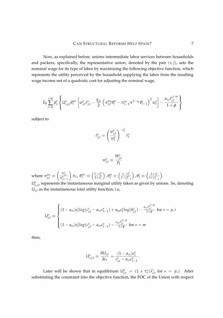
Now, as explained before, unions intermediate labor services between householdsand packers, specifically, the representative union, denoted by the pair (s, j), sets thenominal wage for its type of labor by maximizing the following objective function, whichrepresents the utility perceived by the household supplying the labor from the resultingwage income net of a quadratic cost for adjusting the nominal wage,
E0
+∞
∑t=0
βts
Usc,j,tθ
wct
[ws
j,t`sj,t −
ηw2
(πws
j,t θwt − πιw
t−1π1−ιw θct−1
)2ws
t
]−
a`s`s1+φ
j,t
1+ φ
subject to
`sj,t =
(ws
j,t
wst
)−ε`t
`st
wsj,t ≡
Wsj,t
Pt
where πwsj,t ≡
(ws
j,tws
j,t−1
)πt, θwc
t ≡(
1−τwt
1+τct
), θw
t ≡(
1−τwt
1−τwt−1
), θc
t ≡(
1+τct
1+τct−1
).
Usc,j,t represents the instantaneous marginal utility taken as given by unions. So, denoting
Uj,t as the instantaneous total utility function, i.e,
Usj,t ≡
(1− acs)εz
t log(csj,t − acscs
t−1) + ahsεzt log(hs
j,t)−a`s`s1+φ
j,t1+φ for s = p, i
(1− acs)εzt log(cs
j,t − acscst−1)−
a`s`s1+φ
j,t1+φ for s = m
then,
Usc,j,t ≡
∂Uj,t
∂ct=
(1− acs)εzt
csj,t − acscs
t−1.
Later will be shown that in equilibrium Usj,t = (1 + τc
t )λsj,t for s = p, i. After
substituting the constraint into the objective function, the FOC of the Union with respect

CAN STRUCTURAL REFORMS HELP SPAIN? 8
to type p wage yields
[(1− ε`j,t)`
j,pt − ηw
(π
wpj,t − πιw
t−1π1−ιw)
πwpj,t
]+
a`pε`t `p1+φ
j,t
λpj,t(1−τw)w
pj,t+
βpEt
{λ
pj,t+1
λpj,t
[ηw
(π
wpj,t+1 − πιw
t π1−ιw) π
wp2
j,t+1πt+1
]}= 0.
Since we assume complete markets, we can consider a symmetric equilibrium wherecp
t = cpj,t, hp
t = hpj,t, dt = dp
j,t, λpt = λ
pj,t, and Ut = Uj,t. In addition, following Rotemberg
(1982) we construct a symmetric equilibrium where the wage set by each household isoptimal, given the wages set by other households as well as the expectation of wages thatother households will set in the future. As a consequence, ws
t = wsj,t. Thus, the first order
conditions associated with the patient households’ problem becomes:
λpt (1+ τc)−
(1− acp)εzt
cpt − acpcp
t−1= 0
ahpεht
hpt− λ
pt (1+ τh)qh
t + βpEt
{λ
pt+1(1+ τh)qh
t+1
}= 0
λpt (1+ τ f d)− βpEt
{λ
pt+1
[1+ (1− τd)rd
tπt+1
+ τ f d
]}= 0
[(1− ε`t )`
pt − ηw
(π
wpt − πιw
t−1π1−ιw)
πwpt
]+
a`pε`t `p1+φ
t
λpt (1− τw)w
pt+
βpEt
λpt+1
λpt
ηw
(π
wpt+1 − πιw
t π1−ιw) π
wp2
t+1πt+1
= 0,
where πwpt =
wpt
wpt−1
πt. Using the zero profits condition of the labor packer, wpt lp
t =∫ γp
0 wpj,t`
pj,tdj,
the budget constraint of the patient households can be written as:
(1+ τct )c
pt + (1+ τh
t )qht ∆hp
t + (1+ τf dt )d
pt =
(1− τwt )w
pt `
pt +
[1+(1−τd
t )rdt−1
πt+ τ
f dt
]dp
t−1 +JRt
γp+ (1−ωb)
Jbt−1γp− Tup
tγp− Tg
tγp+γi+γe
.
Finally, the cost of participating in the labor union are equal to the quadratic cost of

CAN STRUCTURAL REFORMS HELP SPAIN? 9
changing the wage
Tupt = γp
ηw2
(π
wpt θw
t − πιwt−1π1−ιw θc
t−1
)2wp
t
2.3 Impatient HouseholdsThere is a continuum of impatient households in the economy indexed by j, with massγi, whose utility function depends on consumption ci
j,t, housing services hij,t and hours
worked `ij,t, and has the following form:
E0
+∞
∑t=0
βti
(1− aci)εzt log(ci
j,t − acicit−1) + ahiε
ht log(hi
j,t)−a`i`i1+φ
j,t
1+ φ
where ci
t denote average patient housholds consumption, i.e,
cit = γ−1
i
(∫ γi
0ci
j,tdj)
;
and εzt and εh
t are defined as in the patient household problem above. The jth impatienthousehold budget constraint, expressed in terms of final goods, is given by:
(1+ τct )c
ij,t + (1+ τh
t )qht ∆hi
j,t +
(1+rbi
t−1πt
)bi
j,t−1 + τf bt ∆bi
j,t =
(1− τwt )w
ij,t`
ij,t + bi
j,t −Tui
tγi− Tg
tγp+γi+γe
.
Impatient households do not hold deposits, and own neither the banks nor the retailfirms. The flow of expenses of impatient households is given by consumption (plus con-sumption taxes) (1+ τc
t )cij,t, housing services (plus housing services taxes) (1+ τh
t )qht ∆hi
j,t,
interest plus principal of loans taken during the previous period(
1+rbit−1
πt
)bi
j,t−1, and taxes
ad-valorem on new lending transactions. The sources of income are labor income (minus
wage taxes) (1− τwt )w
ij,t`
ij,t and loans bi
j,t net of lump-sum fees paid to the unions Tuit
γi, and
lump-sum taxes paid to the government Tgt
γp+γi+γe.
In the last expression, under the same grounds that in the patient households case,we omit the whole set of Arrow-Dereu securities accesible to impatient households.
In addition, impatient households face a borrowing constraint: always in terms offinal goods, they cannot borrow more than a certain proportion of the expected value of

CAN STRUCTURAL REFORMS HELP SPAIN? 10
their housing stock at period t, i.e,
(1+ rbit )b
ij,t ≤ mi
tEt
{qh
t+1hij,tπt+1
},
where mit is the stochastic loan-to-value ratio for mortgages with law of motion:
log mit = (1− ρmi)log mi
ss + ρmilog mit−1 + σmiemi
t where emit ∼ N (0, 1).
We assume that the shocks in the model are small enough so that we can solve themodel imposing that the borrowing constraint always binds as in Iacoviello (2005).
Impatient households choose cit, , hi
j,t, and bij,t (remember that the decision on labor
and wages are delegated on the corresponding labor union) for t = 0, 1, 2, ...,+∞ in orderto maximize its utility function subject to budget and credit constraints. The correspondingLagrangian of this optimization problem is
E0
+∞
∑t=0
βti
(1− aci)εzt log(ci
j,t − acicit−1) + ahiε
zt log(hi
j,t)−a`i`si1+φ
j,t
1+ φ−
λij,t
{(1+ τc
t )cij,t + (1+ τh
t )qht ∆hi
j,t +
(1+ rbi
t−1πt
− τf bt
)bi
j,t−1 − (1− τwt )w
ij,t`
ij,t − (1− τ
f bt )b
ij,t
+Tui
tγi+
Tgt
γp + γi + γe
}− ξ i
j,t
{(1+ rbi
t )bij,t −mi
tEt
{qh
t+1hij,tπt+1
}}],
and the associated first order conditions are
λij,t(1+ τc)−
(1− aci)εzt
cij,t − acici
t−1= 0
ahiεht
hij,t− λi
j,t(1+ τh)qht + ξ i
j,tmij,tEt
{qh
t+1πt+1
}+ βiEt
{λi
j,t+1(1+ τh)qht+1
}= 0
λij,t(1− τ f b)− βiEt
{λi
j,t+1
(1+ rbi
tπt+1
− τ f b
)}− ξ i
j,t(1+ rbit ) = 0.
To determine the optimal values of wij,t and `i
j,t, we should add the first order con-ditions of the union’ optimization problem, derived before, i.e,
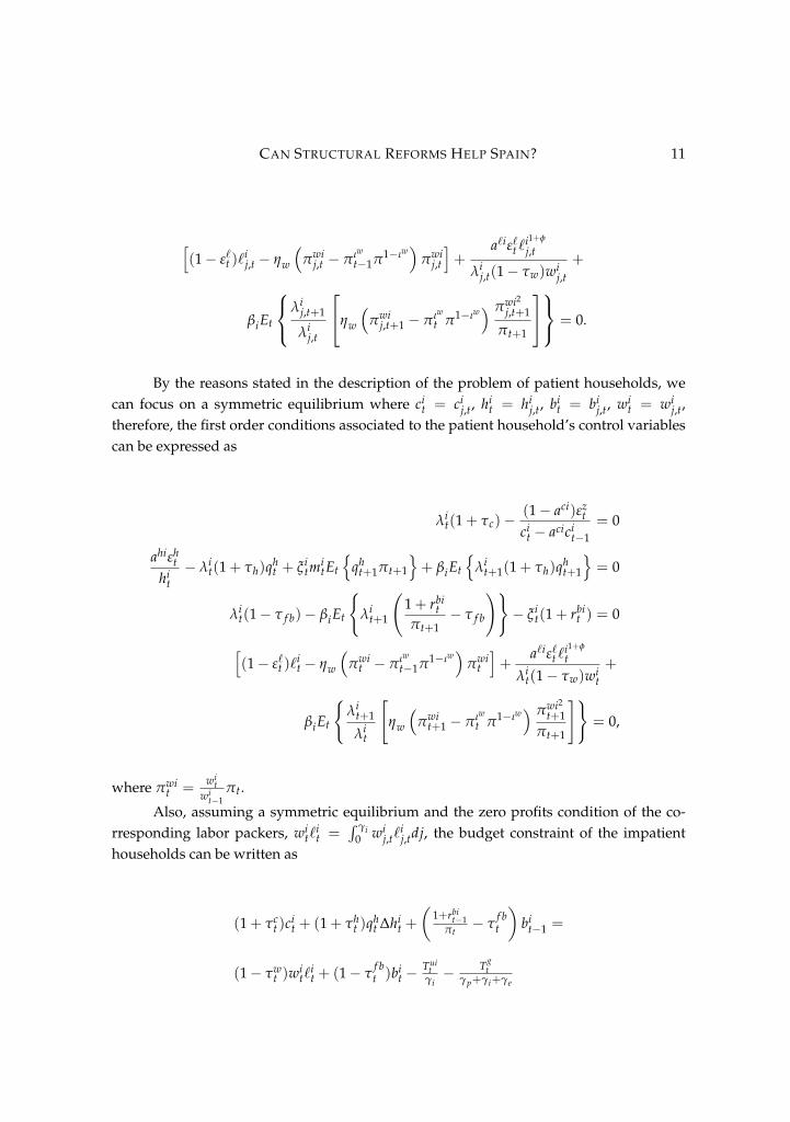
CAN STRUCTURAL REFORMS HELP SPAIN? 11
[(1− ε`t )`
ij,t − ηw
(πwi
j,t − πιw
t−1π1−ιw)
πwij,t
]+
a`iε`t `i1+φ
j,t
λij,t(1− τw)wi
j,t
+
βiEt
λij,t+1
λij,t
ηw
(πwi
j,t+1 − πιwt π1−ιw
) πwi2j,t+1
πt+1
= 0.
By the reasons stated in the description of the problem of patient households, wecan focus on a symmetric equilibrium where ci
t = cij,t, hi
t = hij,t, bi
t = bij,t, wi
t = wij,t,
therefore, the first order conditions associated to the patient household’s control variablescan be expressed as
λit(1+ τc)−
(1− aci)εzt
cit − acici
t−1= 0
ahiεht
hit− λi
t(1+ τh)qht + ξ i
tmitEt
{qh
t+1πt+1
}+ βiEt
{λi
t+1(1+ τh)qht+1
}= 0
λit(1− τ f b)− βiEt
{λi
t+1
(1+ rbi
tπt+1
− τ f b
)}− ξ i
t(1+ rbit ) = 0
[(1− ε`t )`
it − ηw
(πwi
t − πιw
t−1π1−ιw)
πwit
]+
a`iε`t `i1+φ
t
λit(1− τw)wi
t+
βiEt
{λi
t+1
λit
[ηw
(πwi
t+1 − πιwt π1−ιw
) πwi2t+1
πt+1
]}= 0,
where πwit =
wit
wit−1
πt.
Also, assuming a symmetric equilibrium and the zero profits condition of the co-rresponding labor packers, wi
t`it =
∫ γi0 wi
j,t`ij,tdj, the budget constraint of the impatient
households can be written as
(1+ τct )c
it + (1+ τh
t )qht ∆hi
t +
(1+rbi
t−1πt− τ
f bt
)bi
t−1 =
(1− τwt )w
it`
it + (1− τ
f bt )b
it −
Tuit
γi− Tg
tγp+γi+γe

CAN STRUCTURAL REFORMS HELP SPAIN? 12
and the binding borrowing constraint can be written as
(1+ rbit )b
it = mi
tEt
{qh
t+1hitπt+1
};
Finally, the cost of participating in the labor union are equal to the quadratic cost ofchanging the wage
Tuit = γi
ηw2
(πwi
t θwt − πιw
t−1π1−ιw θct−1
)2wi
t.
2.4 Hand-to-mouth HouseholdsThere is a continuum of hand-to-mouth households in the economy indexed by j, withmass γm, whose utility function depends on consumption cm
j,t, and hours worked `ij,t, and
has the following form:
E0
+∞
∑t=0
βtm
(1− acm)εzt log(cm
j,t − acmcmt−1)−
a`m`m1+φ
j,t
1+ φ
.
where cmt denote average hand-to-mouth households consumption, i.e,
cmt = γ−1
m
(∫ γm
0cm
j,tdj)
;
The jth hand-to-mouth household budget constraint is given by:
(1+ τct )c
mi,t = (1− τw
t )wmt `
mi,t −
Tumt
γm.
Hand-to-mouth households do not hold deposits, do not get utility from housingservices, and own neither the banks nor the retail firms. The only expense of hand-to-mouth households is consumption (plus consumption taxes) (1+ τc
t )cmj,t. The sources of
income are labor income, (1− τwt )w
mj,t`
mj,t, net of lump-sum fees paid to the unions, Tum
tγm
.Then, the Lagrangian of hand-to-mouth optimization problem is:
E0
+∞
∑t=0
βtm
(1− acm)εzt log(cm
j,t − acmcmt−1)−
a`m`m1+φ
j,t
1+ φ−
λmj,t
{(1+ τc
t )cmi,t − (1− τw
t )wmt `
mi,t +
Tumt
γm
}].

CAN STRUCTURAL REFORMS HELP SPAIN? 13
where the households maximize over cmj,t (remember that the decision over wages and
labor is delegated on the corresponding labour union) for t = 0, 1, 2, ...,+∞, resulting thefollowing first order condition:
(1+ τc)cmj,t = (1− τw)wm
j,t`mj,t −
Tumt
γm.
The union’s first order conditions wich determine wmj,t and `m
j,t follow the same logicas in the case of patient and impatient households with the obvious modifications, that is,
(1− τw
1+ τc
) [(1− ε`t )`
mt − ηw
(πwm
j,t − πιw
t−1π1−ιw)
πwmt
]+
a`mε`t `m1+φ
j,t
Umc,tw
mt
+
βmEt
Umc,j,t+1
Umc,j,t
ηw
(1− τw
1+ τc
)(πwm
j,t+1 − πιwt π1−ιw
) πwm2
j,t+1
πt+1
= 0
where
Umc,j,t ≡
(1− acm)εzt
cmj,t − acmcm
t−1.
Similar to the case of patient and impatient households, we consider a symmetricequilibrium where cm
t = cmj,t, wm
t = wmj,t, and `m
t = `mj,t. Therefore, the first order conditions
associated to the hand-to-mouth household’s problem become:
(1+ τc)cmt = (1− τw)wm
t `mt −
Tumt
γm(1− τw
1+ τc
) [(1− ε`t )`
mt − ηw
(πwm
t − πιw
t−1π1−ιw)
πwmt
]+
a`mε`t `m1+φ
tUm
c,twmt
+
βmEt
{Um
c,t+1
Umc,t
[ηw
(1− τw
1+ τc
)(πwm
t+1 − πιwt π1−ιw
) πwm2
t+1πt+1
]}= 0
where πwmt =
wmt
wmt−1
πt and
Umc,t ≡
(1− acm)εzt
cmt − acmcm
t−1,
and the budget constraint, again by the packer’s zero profits condition, wmt `
mt =
∫ γm0 wm
j,t`mj,tdj,

CAN STRUCTURAL REFORMS HELP SPAIN? 14
becomes
(1+ τc)cmt = (1− τw)wm
t `mt −
Tumt
γm.
Finally, the cost of participating in the labor union are equal to the quadratic cost ofchanging the wage
Tumt = γm
ηw2
(πwm
t θwt − πιw
t−1π1−ιw θct−1
)2wm
t .
2.5 EntrepreneursThere is a continuum of entrepreneurs in the economy indexed by j, with mass γe, thatchoose consumption ce
j,t, capital kej,t, and loans be
j,t for t = 0, 1, 2, ...,+∞ to maximize thefollowing lifetime utility function
E0
+∞
∑t=0
βte(1− ae)log(ce
j,t − aecet−1).
where cet denotes average entrepreneurs consumption, i.e,
cet = γ−1
e
(∫ γe
0ce
j,tdj)
;
subject to following budget constraint:
(1+ τct )c
ej,t +
(1+rbe
t−1πt
)be
j,t−1 + τf bt ∆be
j,t + qkt ke
j,t =
(1− τkt )r
kt ke
j,t + bej,t + qk
t (1− δ)kej,t−1 +
Jxt
γe+
Jkt
γe− Tg
tγp+γi+γp
.
So, entrepreneurs do not hold deposits, they own the intermediate good producersfirms and the capital good producers firms, but own neither the banks nor the retailfirms. The flow of expenses of entrepreneurs is given by consumption (plus consumptiontaxes) (1 + τc
t )cej,t, capital purchases qk
t kej,t, interest plus principal of loans taken during
the previous period(
1+rbet−1
πt
)be
j,t−1, and taxes on new lending trasactions, τf bt ∆be
j,t. The
sources of income are rental capital (minus capital taxes), (1− τkt )r
kt ke
j,t, loans, bej,t, capital
from the previous period qkt (1 − δ)ke
j,t−1, dividends from intermediate good producers
CAN STRUCTURAL REFORMS HELP SPAIN? 15
Jxt
γe, dividends from capital good producers, Jk
tγe
, and net of lump-sum taxes paid to the
government, Tgt
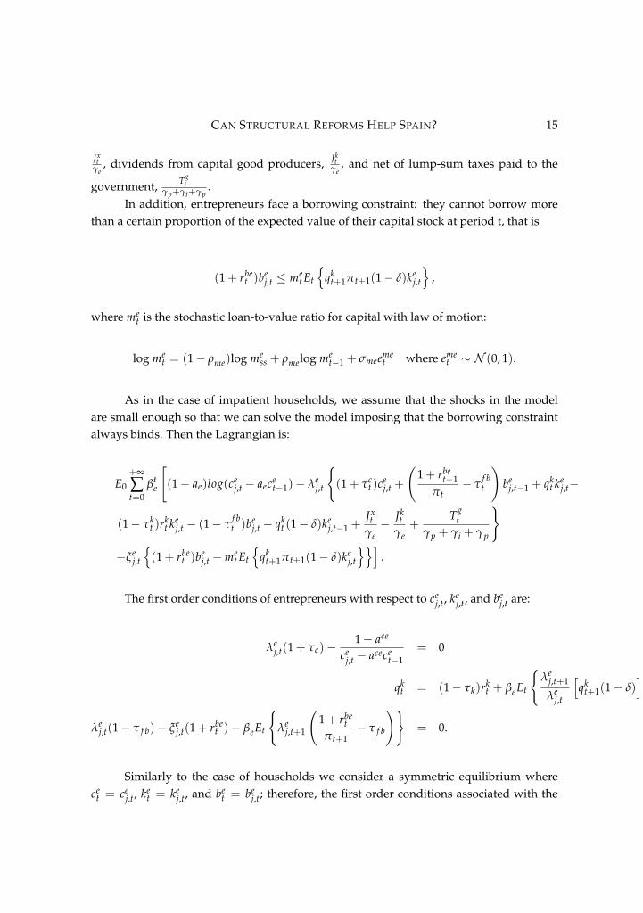
γp+γi+γp.
In addition, entrepreneurs face a borrowing constraint: they cannot borrow morethan a certain proportion of the expected value of their capital stock at period t, that is
(1+ rbet )b
ej,t ≤ me
t Et
{qk
t+1πt+1(1− δ)kej,t
},
where met is the stochastic loan-to-value ratio for capital with law of motion:
log met = (1− ρme)log me
ss + ρmelog met−1 + σmeeme
t where emet ∼ N (0, 1).
As in the case of impatient households, we assume that the shocks in the modelare small enough so that we can solve the model imposing that the borrowing constraintalways binds. Then the Lagrangian is:
E0
+∞
∑t=0
βte
[(1− ae)log(ce
j,t − aecet−1)− λe
j,t
{(1+ τc
t )cej,t +
(1+ rbe
t−1πt
− τf bt
)be
j,t−1 + qkt ke
j,t−
(1− τkt )r
kt ke
j,t − (1− τf bt )b
ej,t − qk
t (1− δ)kej,t−1 +
Jxt
γe− Jk
tγe+
Tgt
γp + γi + γp
}−ξe
j,t
{(1+ rbe
t )bej,t −me
t Et
{qk
t+1πt+1(1− δ)kej,t
}}].
The first order conditions of entrepreneurs with respect to cej,t, ke
j,t, and bej,t are:
λej,t(1+ τc)−
1− ace
cej,t − acece
t−1= 0
qkt = (1− τk)rk
t + βeEt
{λe
j,t+1
λej,t
[qk
t+1(1− δ)]}+
(ξe
j,t
λej,t
)me
t Et
{qk
t+1(1− δ)πt+1
}λe
j,t(1− τ f b)− ξej,t(1+ rbe
t )− βeEt
{λe
j,t+1
(1+ rbe
tπt+1
− τ f b
)}= 0.
Similarly to the case of households we consider a symmetric equilibrium wherece
t = cej,t, ke
t = kej,t, and be
t = bej,t; therefore, the first order conditions associated with the

CAN STRUCTURAL REFORMS HELP SPAIN? 16
entrepreneurs’ problem become:
λet(1+ τc)−
1− ace
cet − acece
t−1= 0
qkt = (1− τk)rk
t + βeEt
{λe
t+1λe
t
[qk
t+1(1− δ)]}+
(ξe
tλe
t
)me
t Et
{qk
t+1(1− δ)πt+1
}λe
t(1− τ f b)− ξet(1+ rbe
t )− βeEt
{λe
t+1
(1+ rbe
tπt+1
− τ f b
)}= 0.
Integrating across entrepreneurs the budget constraint of the entrepreneurs can bewritten as:
(1+ τct )c
et +
(1+rbe
t−1πt− τ
f bt
)be
t−1 + qkt ke
t =
(1− τkt )r
kt ke
t + (1− τf bt )b
et + qk
t (1− δ)ket−1 +
Jxt
γe+
Jkt
γe− Tg
tγp+γi+γp
,
and the binding borrowing constraint can be written as
(1+ rbet )b
et = me
t Et
{qk
t+1πt+1(1− δ)ket
}.
2.6 Intermediate good producersThere is a continuum of intermediate good producers with mass γx. The jth intermediategood producer has access to a technology represented by a production function
yxj,t = At
(kee
j,t−1uj,t
)α [(`
ppj,t
)µp(`ii
j,t
)µi(`mm
j,t
)µm]1−α
(Kg
t−1γx
)αg
,
where keej,t−1 is the capital rented by the firm, uj,t controls how the firm utilizes capital,
`ppj,t is the amount of ˇpackedı patient labor input rented by the firm, `ii
j,t is the amount ofˇpackedı impatient labor input rented by the firm, `mm
j,t is the amount of ˇpackedı hand-to-
mouth labor input rented by the firm, and Kgt−1 is a the amount of public capital controlled
by the government. At denotes an aggregate productivity shock with law of motion:
log At = (1− ρA)log Ass + ρAlog At−1 + σAeAt eA
t ∼ N (0, 1).
In addition, to the cost of the inputs required for production, the intermediate good
producers face a capital utilization cost, ψ(uj,t) ≡[ψu1(uj,t − 1) +
ψu22 (uj,t − 1)2
]kee
j,t−1,

CAN STRUCTURAL REFORMS HELP SPAIN? 17
and a fixed cost of production, Φx. The latter guarantees that the economic profits areroughly equal to zero in the steady state, to be consistent with the additional assumptionof no entry and exit of intermediate good producers.
Intermediate good producers choose keej,t−1, `pp
j,t , `iij,t, `
mmj,t and uj,t for t = 0, 1, 2, ... to
maximize
E0
+∞
∑t=0
βteλe
t
{yx
j,t
xt− wp
t `ppj,t − wi
t`iij,t − wm
t `mmj,t − rk
t keej,t−1 −ψ(uj,t)kee
j,t−1 −Φx,}
,
where xt ≡ PtPx
t, with Px
t the nominal price of intermediate goods, subject to the productionfunction for yx
j,t. Substituting the production function in the objective function we get:
E0
+∞
∑t=0
βteλe
t
At
(kee
j,t−1uj,t
)α [(`
ppj,t
)µp(`ii
j,t
)µi(`mm
j,t
)µm]1−α
(Kg
t−1γx
)αg
xt
−wpt `
ppj,t − wi
t`iij,t − wm
t `mmj,t − rk
t keej,t−1 −
[ψu1(uj,t − 1) +
ψu2
2(uj,t − 1)2
]kee
j,t−1 −Φx
}The first order conditions with respect to `pp
j,t , `iij,t, `
mmj,t ,kee
j,t−1, and uj,t yields
wpt =
µp(1− α)
xt
yxj,t
`ppj,t
wit =
µi(1− α)
xt
yxj,t
`iij,t
wmt =
µm(1− α)
xt
yxj,t
`mmj,t
ψ′(uj,t) =At
xt
(Kg
t−1γe
)αg
α
(`
ppj,t
)µp (`ii
j,t
)µi (`mm
j,t
)µm
keej,t−1uj,t
1−α
rkt = βeEt
{λe
j,t+1
λej,t
[ψ′(uj,t+1)uj,t+1 − ψ(uj,t+1)
]}.
Notice that complete markets imply thatλe
j,t+1λe
j,tis constant, so we can drop the index
j in the first order condition with respect to capital utilization (the last one). Hence, wehave that:

CAN STRUCTURAL REFORMS HELP SPAIN? 18
• Firstly, after integrating out both sides of the first order conditions with respect to j weget
wpt =
µp(1− α)
xt
yxt
`ppt
wit =
µi(1− α)
xt
yxt`ii
t
wmt =
µm(1− α)
xt
yxt
`mmt
rkt = βeEt
{λe
t+1λe
t
[ψ′(ut+1)ut+1 − ψ(ut+1)
]}.
where yxt =
(∫ γx0 yx
j,tdj)
and `sst =
(∫ γx0 `ss
j,tdj)
for all s ∈ {p, i, m}.• Secondy, from the first order conditions it follows that the ratio of capital to labor are
independent of j
keej,t−1
`ppj,t
=α
(1− α)
1µp
wpt
ψ′(ut)
1ut≡ 1
κp,t
keej,t−1
`iij,t
=α
(1− α)
1µi
wit
ψ′(ut)
1ut≡ 1
κi,t
keej,t−1
`mmj,t
=α
(1− α)
1µm
wmt
ψ′(ut)
1ut≡ 1
κm,t.
These expression also imply that
keet−1
`ppt=
1κp,t
keet−1
`iit=
1κi,t
keet−1`mm
t=
1κm,t

CAN STRUCTURAL REFORMS HELP SPAIN? 19
where keet =
(∫ γx0 kee
j,tdj)
.Using the first order condition with respect to capital and the above expression yields
ψ′(ut) =At
xt
(Kg
t−1γx
)αg
α
[(kee
j,t−1κp,t
)µp(
keej,t−1κi,t
)µi(
keej,t−1κm,t
)µm]1−α
(keej,t−1ut)1−α
=At
xt
(Kg
t−1γx
)αg
α1
(keej,t−1)
(1−α)(1−(µp+µi+µm))
[(κp,t)µp (κi,t)
µi (κm,t)µm]1−α
(ut)1−α
=At
xt
(Kg
t−1γx
)αg
α1
(keej,t−1)
αg
[(κp,t)µp (κi,t)
µi (κm,t)µm]1−α
(ut)1−α
=At
xt
(Kg
t−1
)αgα
[(`
ppt
)µp (`ii
t)µi (`mm
t )µm]1−α
(keet−1ut)1−α
where the last line follows from the assumption of constant returns to scale on the pro-duction function, i.e. α+ (µp + µi + µm)(1− α) + αg = 1.
• Thirdly, we can solve for the ratio of private to public capital, which is independent ofj
keej,t−1
Kgt−1
=
1ψ′(ut)
At
xtα
[(κp,t,
)µp (κi,t)µi (κm,t)
µm]1−α
(ut)1−α
1
αg (1
γx
).
Hencekee
t−1Kg
t−1=
keej,t−1γx
Kgt−1
.
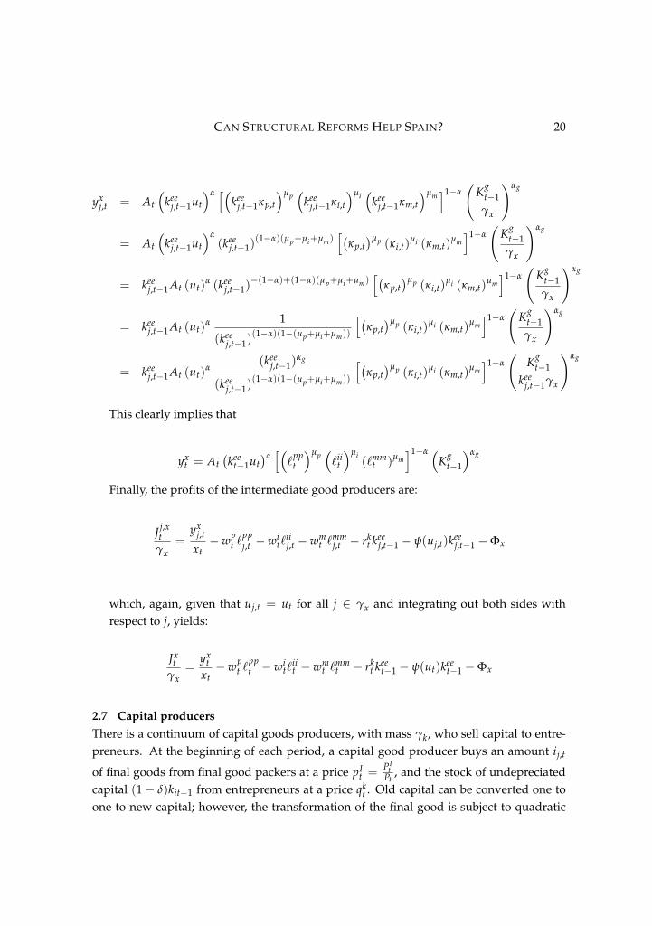
Substituting these ratios into the production function yields
CAN STRUCTURAL REFORMS HELP SPAIN? 20
yxj,t = At
(kee
j,t−1ut
)α [(kee
j,t−1κp,t
)µp(
keej,t−1κi,t
)µi(
keej,t−1κm,t
)µm]1−α
(Kg
t−1γx
)αg
= At
(kee
j,t−1ut
)α(kee
j,t−1)(1−α)(µp+µi+µm)
[(κp,t)µp (κi,t)
µi (κm,t)µm]1−α
(Kg
t−1γx
)αg
= keej,t−1 At (ut)
α (keej,t−1)
−(1−α)+(1−α)(µp+µi+µm)[(
κp,t)µp (κi,t)
µi (κm,t)µm]1−α
(Kg
t−1γx
)αg
= keej,t−1 At (ut)
α 1
(keej,t−1)
(1−α)(1−(µp+µi+µm))
[(κp,t)µp (κi,t)
µi (κm,t)µm]1−α
(Kg
t−1γx
)αg
= keej,t−1 At (ut)
α(kee
j,t−1)αg
(keej,t−1)
(1−α)(1−(µp+µi+µm))
[(κp,t)µp (κi,t)
µi (κm,t)µm]1−α
(Kg
t−1kee
j,t−1γx
)αg
This clearly implies that
yxt = At
(kee
t−1ut)α[(`
ppt
)µp(`ii
t
)µi(`mm
t )µm]1−α (
Kgt−1
)αg
Finally, the profits of the intermediate good producers are:
J j,xt
γx=
yxj,t
xt− wp
t `ppj,t − wi
t`iij,t − wm
t `mmj,t − rk
t keej,t−1 − ψ(uj,t)kee
j,t−1 −Φx
which, again, given that uj,t = ut for all j ∈ γx and integrating out both sides withrespect to j, yields:
Jxt
γx=
yxt
xt− wp
t `ppt − wi
t`iit − wm
t `mmt − rk
t keet−1 − ψ(ut)kee
t−1 −Φx
2.7 Capital producersThere is a continuum of capital goods producers, with mass γk, who sell capital to entre-preneurs. At the beginning of each period, a capital good producer buys an amount ij,t
of final goods from final good packers at a price pIt =
PIt
Pt, and the stock of undepreciated
capital (1− δ)kit−1 from entrepreneurs at a price qkt . Old capital can be converted one to
one to new capital; however, the transformation of the final good is subject to quadratic

CAN STRUCTURAL REFORMS HELP SPAIN? 21
adjustment costs. Accordingly, the law of motion for capital, is
k j,t = (1− δ)k j,t−1 +
1− ηi2
(ij,tε
kt
ij,t−1− 1
)2 ij,t,
where εkt has the following law of motion:
log εkt = (1− ρεk)log εk
ss + ρεklog εkt−1 + σkek
t ekt ∼ N (0, 1).
The new capital stock is then sold back to entrepreneurs at a price equal to qkt . There
is also a fixed cost of being a capital goods producer in order to guarantee that the profitsare roughly zero around the steady state. Then, each capital good producer chooses k j,t
and ij,t for t = 0, 1, 2, ...,+∞ to maximize:
E0
+∞
∑t=0
βteλe
t
{qk
t [k j,t − (1− δ)k j,t−1]− pIt ij,t −Φk
}subject to the law of motion for capital. After substituting the constraint and taking theFOC with respect to ij,t we get:
qkt
[1− ηi
2
(ij,tε
kt
ij,t−1− 1)2− ηi
(ij,tε
kt
ij,t−1− 1)(
εkt
ij,t−1
)ij,t
]+
βeEt
{λe
j,t+1λe
j,t
[qk
t+1εkt+1ηi
(ij,t+1εk
t+1ij,t
− 1)( ij,t+1
ij,t
)2]}
= pIt .
By the assumption of complete marketsλe
j,t+1λe
j,tso that it = ij,t, and we can drop the
subindex j in the previous equation
qkt
[1− ηi
2
(itεk
tit−1− 1)2− ηi
(itεk
tit−1− 1)(
εkt
it−1
)it
]+
βeEt
{λe
t+1λe
t
[qk
t+1εkt+1ηi
(it+1εk
t+1it− 1)(
it+1it
)2]}
= pIt ,
and in the law of motion for capital
kt = (1− δ)kt−1 +
1− ηi2
(itε
kt
it−1− 1
)2 it.

CAN STRUCTURAL REFORMS HELP SPAIN? 22
Then, the profits of capital good producers are:
Jkt
γk= qk
t
1− ηi
2
(itε
kt
it−1− 1
)2 it
− pIt it −Φk.
2.8 Home Goods RetailersThere is a continuum of final goods retailers, with mass γ, operating in a monopolisticallycompetitive market. Each good retailer buys an amount of the homogeneous intermediategood sold by intermediate goods producers, differentiates it and sells the resulting vari-eties at a mark-up over its marginal cost to ˇhome-produced final goods packersı who in turnbundle the varieties together and sell the home-produced final homogeneous good to "finalgoods packers" that bundle home and imported production.
We assume that retail prices are indexed by a combination of past and steady stateinflation with relative weights parameterized by ιp. In addition, retailers are subject toquadratic price adjustment costs, where ηp controls the size of these costs.
Then, each retailer chooses the nominal price for its differentiated home producedgood, PH
j,t , for t = 0, 1, 2, ...,+∞ to maximize:
E0
+∞
∑t=0
βtpλ
pt PH
t
PHj,t yj,t
PHt−
yxxj,t
xt−
ηp
2
(PH
j,t
PHj,t−1−(
πHt−1
)ιp (πH
ss
)1−ιp
)2
Yt
subject to
yj,t = yxxj,t
yj,t =
(PH
j,t
PHt
)−εyt
Yt
where πHt is the gross inflation of PH
t and εyt is the elasticity of substitution which follows
an AR(1) process with law of motion:
log εyt = (1− ρεy)log ε
yss + ρεylog ε
yt−1 + σyey
t eyt ∼ N (0, 1).
The demand faced by retailers is derived from the optimization problem solved byretail goods packers, left implicit.
CAN STRUCTURAL REFORMS HELP SPAIN? 23
The first order condition of the intermediate goods producer’s problem is:
1− εyt +
εyt
xt− ηpπH
t
(πH
t −(πH
t−1)ιp (πH
ss)1−ιp
)+
βpEt
{λ
pt+1λ
pt
[(πH
t+1)2(
Yt+1Yt
)ηp
(πH
t+1 −(πH
t)ιp (πH
ss)1−ιp
)]}= 0.
We have omitted the subindeces in the first order condition because of completemarkets and the construction of a symmetric equilibrium as in the case of the patienthouseholds, which also imply that PH
j,t = PHt and henceforth that
Yt =
∫ γ
0y
εyt
1−εyt
j,t dj
1−ε
yt
εyt
.
Finally, the retailers aggregate profits are:
JRt = Yt
[1− 1
xt−
ηp
2
(πH
t −(
πHt−1
)ιp (πH
ss
)1−ιp)2]
.
2.9 BanksBanks play a key role in the model by intermediating financial transactions between theagents. In the model there is a continuum of them, with mass γb, composed by three partseach one: a wholesale unit and two ˇretailı branches. The two retail branches are responsi-ble for giving out differentiated loans and raising differentiated deposits from householdsand entrepreneurs, and are assumed to operate in monopolistically competitive markets.Specifically, each unit of deposits and loan contract bought by households and entrepre-neurs are a CES basket of slightly differentiated products supplied by each branch j, withpackers intermediating the transactions and exploiting the market power derived formdifferentiation. The wholesale unit manages the capital position of the group, receivesloans form abroad, and raises wholesale domestic loans and deposits in the interbankmarket.
Banks: Wholesale branch
There is a continuum of wholesale banks with mass γb. The representative wholesalebank combine bank capital, kb
j,t, wholesale deposits, dbj,t, and foreign borrowing, − B∗t
γb,
in order to issue wholesale domestic loans, bbj,t, everything expressed in terms of final
consumption goods. The wholesale banks face costs on the wholesale activity related to

CAN STRUCTURAL REFORMS HELP SPAIN? 24
their capital position. Specifically, the banks pay a quadratic cost whenever the capital-
to-assets ratiokb
j,t
bbj,t
deviates from an exogenously given target. In addition, the banks must
satisfy a balance sheet constraint linking equity, liabilities, and assets, i.e.
bbj,t = db
j,t −B∗tγb+ kb
j,t,
Finally, bank capital, in nominal terms, kbj evolves according to the following law of motion
kbj,t =
(1− δb)
εkbt
kbj,t−1 +ωb jb
j,t−1,
where εkbt is a shock to the capital stock and jb
j,t represents the aggregate consolidatedprofits in nominal terms of the j-th bank holding in the economy from the deposit and
loan contracts delivered at period t. Reexpressed in terms of kbj,t ≡
kbj,t
Ptand jb
j,t ≡jbj,tPt
, i.e,capital and profits in consumption good units, the latter expression becomes
Ptkbj,t =
(1− δb)
εkbt
Pt−1kbj,t−1 +ωbPt jb
j,t−1,
or, equivalently,
πtkbj,t =
(1− δb)
εkbt
kbj,t−1 +ωbπt jbj,t−1.
Finally εkbt follows the following law of motion,
log εkbt = (1− ρεkb)log εkb
ss + ρεkblog εkbt−1 + σkbekb
t with ekbt ∼ N (0, 1).
Given these definitions, the problem of the j-th wholesale bank is to choose theamount of wholesale loans, bb
j,t, and wholesale deposits, dbj,t, for t = 0, 1, 2, ...,+∞ in order
to maximize the present value of intertemporal cash flows or, equivalently, by substitutingthe balance sheet equation into the latter expression the problem becomes one of uncon-strained maximization of the following objective function,
maxbb
j,t ,dbj,t ,B
∗t
rbt bb
j,t − rtdbj,t + r∗t
B∗tγb− ηb
2
(kb
j,t
bbj,t− νb
)2
kbj,t
where rbt , rt and r∗t are the nominal gross interest rates for wholesale lending, domestic

CAN STRUCTURAL REFORMS HELP SPAIN? 25
fund rising and foreign borrowing, respectively, all of them taken as given by wholesalebanks. The rate rt is also the monetary policy rate what follows, in equilibrium, from theassumption that wholesale banks count on full-allotment availability of funds from themonetary authority at that rate. The first order condition displays the following results:
(rbt − rt) = −ηb
(kb
t
bbt− νb
)(kb
t
bbt
)2
(1)
(rbt − r∗t ) = −ηb
(kb
t
bbt− νb
)(kb
t
bbt
)2
(2)
We can drop the subindex j from the first order conditions because we focus on a symmet-ric equilibrium where each wholesale unit j decides its optimal capital to loans ratio takingas given the capital to loans ratio of other banks. Accordingly, we can drop the subindicesfrom the law of motion for bank capital yielding
πtkbt =
(1− δb)
εkbt
kbt−1 +ωb
(πt Jb
t−1γb
),
and the balance sheet equation of each wholesale unit
bbt = db
t −B∗tγb+ kb
t .
where Jbt is the aggregate of the consolidated profits for the γb bank holdings which
populate the economy.Following Schmitt-Grohé and Uribe (2003), to ensure stationarity of equilibrium we
assume that banks pay a risk-premium that increases with the country’s net foreign assetposition. Thus, we close the model by assuming that the rate r∗t is equal to the exogenousinterest rate r∗∗ multiplied by a risk premium
r∗t = φtr∗∗ (3)
where the risk premium φt increases with the deviation (in absolute value) of the ratio ofnet foreign asset position to output with respect to a constant b∗
φt = exp(−φ
(B∗tYt− b∗
)θ
rpt
)(4)

CAN STRUCTURAL REFORMS HELP SPAIN? 26
and the shock θrpt obeys the following law of motion
log θrpt = (1− ρθrp)log θ
rpss + ρθrplog θ
rpt−1 + σrp erp
t with erpt ∼ N (0, 1)
Notice that equations (1), (2), and (3) imply that
rt = φtr∗∗t
Banks: Deposit-retailing branch
There is a continuum of deposit-retailing banks with mass γb. Each retailing-deposit banksells a differentiated type of deposit to ˇdeposit packersı who bundle the deposits boughtto all deposit-retailing banks according to a CES production function and sell the packeddeposits to patient households. Finally, each deposit-retailing bank uses its resources tofund the wholesale unit at the monetary policy interest rate rt.
The jth deposit-retailing bank chooses the path of the nominal gross interest ratepaid by its type of deposit, rd
j,t for t = 0, 1, 2, ...,+∞, in order to maximize:
E0
+∞
∑t=0
βtpλ
pt
rtdbj,t − rd
j,tdppj,t −
ηp
2
(rd
j,t
rdj,t−1− 1
)2
rdt dpp
t
subject to
dbj,t = dpp
j,t
dppj,t =
(rd
j,t
rdt
)−εdt
dppt ,
The last expression corresponds to the packers’ demand for the type of depositsupplied by the jth deposit-retailing bank1, where εd
t is the elasticity of substitution be-
tween types of deposit. In practice, we reparameterize this elasticity as εdt ≡
(θd
tθd
t−1
)with
θdt , which is related to the flexible prices mark-down charged by deposit-retailing banks
relative to the monetary policy rate, obeying the following law of motion:
1 The derivation of this demand is analogous to the one for the labor packers described above.

CAN STRUCTURAL REFORMS HELP SPAIN? 27
log θdt = (1− ρθd)log θd
ss + ρdlog θdt−1 + σded
t with edt ∼ N (0, 1).
From the first order condition we get the following equilibrium condition for therepresentative deposit-retailing bank:
1+ rtrd
t
(θd
tθd
t−1
)−(
θdt
θdt−1
)+ ηp
(rd
trd
t−1− 1)
rdt
rdt−1
−βpEt
{λ
pt+1λ
pt
[ηp
(rd
t+1rd
t− 1)(
rdt+1rd
t
)2dpp
t+1dpp
t
]}= 0.
where the index j has been dropped from the first order condition because of completemarkets and the consideration of a symmetric equilibrium (see Rotemberg, 1982). Thus,
dbt = dpp
t .
Banks: Loan-retailing branch
There is a continuum of loan-retailing banks with mass γb. Each loan-retailing bankborrows wholesale loans from the wholesale unit at a rate rb
t , and sells a differentiated typeof loan to ˇloan packersı who bundle the loans bought to all loan-retailing banks accordingto a CES production function and finally sell the packed loans to impatient households andentrepreneurs.
The jth loan-retailing bank chooses the nominal gross interest rates for its loansto impetient households, ri
j,t, and entrepreneurs, rej,t, for t = 0, 1, 2, ...,+∞, in order to
maximize:
E0
+∞
∑t=0
βtpλ
pt
rbij,tb
iij,t + rbe
j,tbeej,t + θ
gssrb
t
(Bg
tγb
)− rb
t bbj,t −
ηi2
(rbi
j,t
rbij,t−1− 1
)2
rbit bii
t −ηe2
(rbe
j,t
rbej,t−1− 1
)2
rbet bee
t
subject to
bbj,t = bii
j,t + beej,t +
Bgt
γb,

CAN STRUCTURAL REFORMS HELP SPAIN? 28
biij,t =
(rbi
j,t
rbit
)−εbit
biit ,
and
beej,t =
(rbe
j,t
rbet
)−εbet
beet .
The last two expressions correspond to the loan packers’ demand for the type ofloans supplied by the jth loan-retailing bank2, where εbi
t and εbet are the elasticities of
substitution between types of loans for impatient households and for entrepreneurs, re-
spectively. In practice, we reparameterize these elasticities as εbst ≡
(θbs
tθbs
t −1
)for s = i, e
with θbst , which is related to the flexible prices mark-up charged by loan-retailing banks
relative to the monetary policy rate, obeying the following law of motion:
log θbst = (1− ρθbs)log θd
ss + ρdlog θbst−1 + σbsebs
t with ebst ∼ N (0, 1).
The first order conditions for this problem are:
1+ rbt
rbit
(θbi
tθbi
t −1
)−(
θbit
θbit −1
)− ηbi
(rbi
trbi
t−1− 1)
rbit
rbit−1+ βpEt
{λ
pt+1λ
pt
[ηbi
(rbi
t+1rbi
t− 1)(
rbit+1rbi
t
)2bii
t+1bii
t
]}= 0
1+ rbt
rbet
(θbe
tθbe
t −1
)−(
θbet
θbet −1
)− ηbe
(rbe
trbe
t−1− 1)
rbet
rbet−1+ βpEt
{λ
pt+1λ
pt
[ηbe
(rbe
t+1rbe
t− 1)(
rbet+1rbe
t
)2bee
t+1bee
t
]}= 0
where again we dropped the subindex j from the individual first order condition becauseof the reasons mentioned above. It allows also to write,
bbt = bii
t + beet +
Bgt
γb.
2 The derivation of these demands, as in the case of the deposit packers, is analogous to the one for the laborpackers described above.

CAN STRUCTURAL REFORMS HELP SPAIN? 29
Bank holding’s profits
The consolidated profit of the j-th bank holding in consumption good units is given by
jbj,t = rbi
t biit + rbe
t beet + θ
gssrb
t
(Bg
tγb
)− rd
t dppt + r∗t
B∗tγb− ηb
2
(kb
tbb
t− νb
)2kb
t
− ηd2
(rd
trd
t−1− 1)2
rdt dt − ηbi
2
(rbi
trbi
t−1− 1)2
rbit bii
t −ηbe2
(rbe
trbe
t−1− 1)2
rbet bee
t .
2.10 External SectorWe consider a world of two asymmetric countries in which the home country is smallrelative to the other (the rest of the world), whose equilibrium is in the limit taken asexogenous (see Monacelli, 2003 or Galí and Monacelli, 2005). As the price numeraire isbefore tax CPI, we define relative prices below in lower case.
Imports
We assume that there is a continuum of final consumption good packers with mass γc
that buy domestic chjt and foreign c f
jt consumption goods, pack them and sell the bundle tohouseholds and entrepreneurs. The aggregation technology is expressed by the followingCES composite baskets of home and foreign produced goods.
ccjt =
((1−ωc)
1σc
(ch
jt
) σc−1σc +ωc
1σc
(c f
jt
) σc−1σc
) σcσc−1
(5)
Similarly, we consider the existence of a continuum of final investment packers withmass γz that buy domestic ih
jt and foreign i fjt investment goods, pack them and sell the
bundle to capital producers. The technology is given by
izjt =
((1−ωi)
1σi
(ihjt
) σi−1σi +ωi
1σi
(i fjt
) σi−1σi
) σiσi−1
(6)
where σc and σi are the consumption and investment elasticities of substitution betweendomestic and foreign goods and ωc , ωi is inversely related with the degree of home biasand, therefore, of openess.
Each period, the consumption packer chooses chjt and c f
jt to minimize productioncosts subject to the technological constraint given by (5). The Lagrangian of this problem
CAN STRUCTURAL REFORMS HELP SPAIN? 30
can be written as:
minch
jt , c fjt
{(PH
t chjt + PM
t c fjt
)
+Pt
ccjt −
((1−ωc)
1σc
(ch
jt
) σc−1σc +ωc
1σc
(c f
jt
) σc−1σc
) σcσc−1
(7)
where PHt and PM
t are respectively the prices of home and foreign produced goods (ex-pressed in domestic currency and including import tariffs). Note that Pt represents boththe consumer price index (CPI) before the consumption tax and the shadow cost of pro-duction of a final good faced by the aggregator.
The optimal allocation of aggregate consumption between domestic and foreigngoods, ch
jt and c fjt, satisfies the following conditions:
chjt = (1−ωc)
(pH
t
)−σccc
jt (8)
c fjt = ωc
(pM
t
)−σccc
jt (9)
Similarly, the investment distributor chooses ihjt and i f
jt to minimize production costssubject to the technological constraint given by (6) by minimizing the Lagrangian
minIht ,I f t
{(PH
t ihjt + PM
t i fjt
)
+PIt
izjt −
((1−ωi)
1σi
(ihjt
) σi−1σi +ωi
1σi
(i fjt
) σi−1σi
) σiσi−1 (10)
from which the demand for home and foreign investment goods are obtained
ihjt = (1−ωi)
(pH
tpI
t
)−σi
izjt (11)
i fjt = ωi
(pM
tpI
t
)−σi
izjt (12)
By assuming a symmetric equilibrium we can drop the subindex j from previousequations to get

CAN STRUCTURAL REFORMS HELP SPAIN? 31
cht = (1−ωc)
(pH
t
)−σccc
t (13)
c ft = ωc
(pM
t
)−σccc
t (14)
iht = (1−ωi)
(pH
tpI
t
)−σi
izt (15)
i ft = ωi
(pM
tpI
t
)−σi
izt (16)
In order to obtain the expression behind the CPI, the demands for home and foreignconsumption goods need to be incorporated into the cost of producing final consumptiongoods (Ptct = PH
t cht + PM
t c ft ). Bearing in mind that the unitary production cost for the
distributor is equal to the price of producing one unit of the packed good, the consumptionand investment price index (before consumption and investment tax/subsidy) can be expressedas a function of the domestic and import deflators3
Pt =
((1−ωc)
(PH
t
)1−σc+ωc
(PM
t
)1−σc) 1
1−σc(17)
PIt =
((1−ωi)
(PH
t
)1−σi+ωi
(PM
t
)1−σi) 1
1−σi(18)
Let’s define CPI gross inflation as πt =Pt
Pt−1and the after consumption tax inflation
as π′t =Pt
Pt−1
1+τct
1+τct−1
. This will be the inflation monitorized by the Central Bank. The twoprevious equations can be written in relative terms as
1 =((1−ωc)
(pH
t
)1−σc+ωc
(pM
t
)1−σc) 1
1−σc(19)
3 Under the assumption that ωc = ωi and σc = σi the consumption and investment price indexes are the same(this is the approach in Farhi et al, 2011 or Stähler and Thomas, 2012).

CAN STRUCTURAL REFORMS HELP SPAIN? 32
pIt =
((1−ωi)
(pH
t
)1−σi+ωi
(pM
t
)1−σi) 1
1−σi(20)
Given the small open economy assumption, the price of imports in domestic cur-rency is defined as:
pMt = ert(1+ τm
t ) (21)
where ert is the real exchange rate (and ERt the nominal exchange rate), i.e., ert =ERtP∗t
Pt,
τmt represents the import tariff4 and P∗t stands for the exogenous world price index.
Some aggregate definitions follow from the previous equations
Ct = γccct (22)
Cht = γccht (23)
It = γzizt (24)
Iht = γziht (25)
and total imports are
IMt = γcc ft + γzi f
t = C f t + I f t (26)
Therefore, the following equalities hold in aggregate
Ct = γccct = pH
t γccht + pM
t γcc ft = γpcp
t + γicit + γece
t + γmcmt (27)
It = γzizt =
pHt
pIt
γziht +
pMt
pIt
γzi ft = γkit (28)
4 In a full monetary union the tariff rate is zero.

CAN STRUCTURAL REFORMS HELP SPAIN? 33
Exports
Export prices set by domestic firms could deviate from competitors’ prices in foreignmarkets (there is some degree of imperfect exchange rate pass through). To make thisassumption operational, we can think of a fraction (1− ptm) of retailing firms whoseprices at home and abroad differ. The remaining fraction of firms, ptm, trade goods freelysetting a unified price across countries (i.e., the law of one price holds). Thus, the exportprice deflator is defined as
pEXt = (1− τx
t )pH(1−ptm)t (ert)
ptm (29)
where pEXt is the export price deflator, τx
t is an export subsidy and the parameter ptmdetermines the degree of pass through.
A set of analogous optimality conditions characterize the solution to the consumer’sproblem in the world economy, where a continuum Dixit-Stiglitz aggregators with massγ∗ faces a problem identical to the one outlined above for consumption and investment5.The symetric conditions for foreign consumption of home-produced goods are therefore
c∗ ft = ω∗c
(pEX
tert
)−σ∗cc∗t (30)
i∗ ft = ω∗c
(pEX
tert
)−σ∗ci∗t (31)
where c∗t and i∗t represent the (exogenous) consumption and investment demand in theworld economy. Therefore, exports of the home economy ext = c∗ f
t + i∗ ft can be written
as
ext = ω∗c
(pEX
tert
)−σ∗c(c∗t + i∗t ) (32)
Plugging (29) into (32) yields the exports demand for a small open economy
ext = ω∗c
((1− τx
t )
(pH
tert
)(1−ptm))−σ∗c
(c∗t + i∗t ) (33)
Note that with full pricing to market (ptm = 0), pEXt = (1− τx
t )pHt and expression (32)
5 For simplicity, we assume that the CES basket is the same for consumption and investment.

CAN STRUCTURAL REFORMS HELP SPAIN? 34
simplifies to
ext = ω∗c
((1− τx
t )
(pH
tert
))−σ∗c(c∗t + i∗t ) (34)
Conversely, if the law of one price holds for all consumption and investment goods, thenptm = 1, pEX
t = (1− τxt )ert and expression (32) simplifies to
ext = ω∗c (1− τxt )−σ∗c (c∗t + i∗t ) (35)
Thus, if the law of one price holds, exports are a sole function of total aggregateconsumption and investment from abroad. Under full pricing to market (ptm = 0),exports are also a function of relative prices with elasticity σ∗c . Under the more generalcase of partial pricing-to-market (0 < ptm < 1),the price elasticity of exports is given(1− ptm) σ∗c .
Finally, we can define aggregate exports as
EXt = γ∗ext (36)
Accumulation of foreign assets
The net foreing asset position B∗t evolves according to the following expression (denomi-nated in the home currency)
B∗t =
(1+ r∗t−1
)πt
B∗t−1 +[
pEXt γ∗ext − pM
t
(γcc f
t + γzi ft
)](37)
where a negative/positive sign for B∗t implies a borrowing/lending position for the do-mestic economy with respect to the rest of the world and r∗t stands for the interest ratepaid/received for borrowing/lending abroad. Also, trade balance TBt is defined as
TBt = pEXt γ∗ext − pM
t
(γcc f
t + γzi ft
)(38)
2.11 Monetary authorityThe home economy belongs to a monetary union (say EMU), and monetary policy ismanaged by the central bank (say ECB) through the following Taylor rule that sets thenominal area-wide reference interest rate allowing for some smoothness of the interest
CAN STRUCTURAL REFORMS HELP SPAIN? 35
rate response to the inflation and output
(1+ rt) = (1+ rss)(1−φr)(1+ rt−1)
φr
(πemu
tπemu
ss
)φπ(1−φr)(
yemut
yemut−1
)φy(1−φr)
(1+ ert)
where πemut is the EMU inflation as measured in terms of the consumption price deflator
and yemut
yemut−1
measures the gross rate of growth of EMU output. There is also some inertia innominal interest rate setting.
The home economy contributes to EMU inflation and output growth according toits economic size in the euro zone, ωSp:
πemut = (1−ωSp)
(πremu
t ε∗πt
)+ωSpπ′t (39)
yemut
yemut−1
= (1−ωSp)
(yremut
yremut−1
)ε∗yt
+ωSpyt
yt−1(40)
where πremut and
(yremu
tyremu
t−1
)are average inflation and output growth in the rest of the Euro-
zone that are subject to shocks modeled according to the following law of motion
log ε∗πt = (1− ρθrp)log ε∗πss + ρθrplog ε∗πt−1 + σrp e∗πt with e∗πt ∼ N (0, 1)
log ε∗yt = (1− ρθrp)log ε
∗yss + ρθrplog ε
∗yt−1 + σrp e∗yt with e∗yt ∼ N (0, 1)
However, instead of a Taylor rule we use the following condition to detrmine thedomestic interest rate
rt = φrr∗t (41)
where φr is a parameter that relates the rate of borrowing abroad and the domestic interestrate.
The real exchange rate is given by the ratio of relative prices between the domesticeconomy and the remaining EMU members, so real appreciation/ depreciation develop-ments are driven by the inflation differential of the domestic economy vis-à-vis the euroarea:
ert+1
ert=
πremut+1
πt+1(42)

CAN STRUCTURAL REFORMS HELP SPAIN? 36
2.12 Fiscal authority’s budget ConstraintThere is also a fiscal authority with a flow of expenses determined by consumption, invest-ment on public capital, and interest plus principal borrowed during the previous period.The fiscal authority collects revenues with new debt, lump-sum taxes, and distortionarytaxation on consumption, housing services, labor income, loans, and deposits.
Cgt + Ig
t +
(1+θb
ssrbt−1
πt
)Bg
t−1 = Bgt + Tg
t + τct
[γpcp
t + γicit + γece
t + γmcmt
]+
τmt
1+τmt
pMt IMt − τx
t1−τx
tpEX
t EXt
+ τht qh
t
[γp
(hp
t − hpt−1 )+γi( hi
t − hit−1
)]+ τw
t
[wp
t γp`pt + wi
tγi`it + wm
t γm`mt
]+ τk
t rkt Kt
+ τf bt[γi(b
it − bi
t−1)) + γe(bet − be
t−1))]+ τ
f dt γp(d
pt − dp
t−1) + τdt
(rd
t−1πt
)γpdp
t−1.
Tax rates are determined according to the following fiscal policy rule
τst = τs for s = c, h, w, d, f d, f b, r, m, x.
ψbgt ≡
(Bg
tγyt
)
ψcgt ≡
(Cg
tγyss
)
ψigt ≡
(Igt
γyss
)
ψtg ≡(
Tgt
γyss
)
ψcgt = (1− ρcg)ψ
cgss + ρcgψ
cgt−1 + σcgecg
t
ψigt = (1− ρig)ψ
igss + ρigψ
igt−1 + σigeig
t
ψtgt = ψ
tgt−1 + ρtgb1
(ψ
bgt − ψ
bgss
)+ ρtgb2
(ψ
bgt − ψ
bgt−1
)Finally, public capital evolves according to the law of motion
Kgt = (1− δg)K
gt−1 + Ig
t .
CAN STRUCTURAL REFORMS HELP SPAIN? 37
2.13 Aggregation and market clearing in equilibrium
Factors of production markets
The supply of labor by each category of household equals the corresponding demand forit from intermediate good producers, i.e.,
∫ γp
0`
pj,tdj =
∫ γx
0`
ppj,t dj⇒ γp`
pt = γx`
ppt
∫ γi
0`i
j,tdj =∫ γx
0`i
j,tdj⇒ γi`it = γx`
iit
∫ γm
0`m
j,tdj =∫ γx
0`m
j,tdj⇒ γm`mt = γx`
mmt ,
The supply of physical capital units by capital producers equals the correspondingdemand by entrepreneurs, while the supply of physical capital rental services by the latterequals the demand of these services by intermediate good producers, i.e.,
∫ γe
0ke
j,tdj =∫ γk
0k j,tdj⇒ γeke
t = γkkt,
∫ γx
0kee
j,tdj =∫ γe
0ke
j,tdj⇒ γxkeet = γeke
t ,
Housing market
The demand for houses by households equals a perfectly inelastic supply of houses,
∫ γx
0hi
j,tdj+∫ γx
0hp
j,tdj = Ht ⇒ γphpt + γih
it = Ht,
Intermediate goods
The demand of intermediate goods by final good producers or retailers equals the supplyof them by intermediate good producers,
CAN STRUCTURAL REFORMS HELP SPAIN? 38
∫ γx
0yx
j,tdj =∫ γ
0yxx
j,t dj⇒ γxyxt = γyt
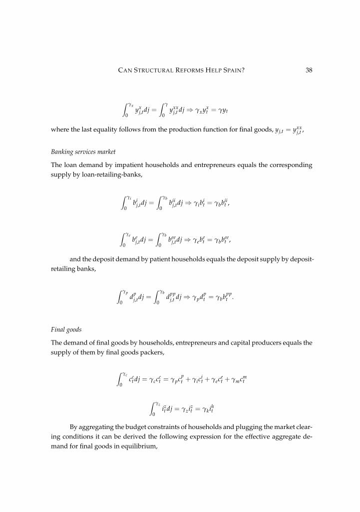
where the last equality follows from the production function for final goods, yj,t = yxxj,t ,
Banking services market
The loan demand by impatient households and entrepreneurs equals the correspondingsupply by loan-retailing-banks,
∫ γi
0bi
j,tdj =∫ γb
0bii
j,tdj⇒ γibit = γbbii
t ,
∫ γe
0be
j,tdj =∫ γb
0bee
j,tdj⇒ γebet = γbbee
t ,
and the deposit demand by patient households equals the deposit supply by deposit-retailing banks,
∫ γp
0dp
j,tdj =∫ γb
0dpp
j,t dj⇒ γpdpt = γbbpp
t .
Final goods
The demand of final goods by households, entrepreneurs and capital producers equals thesupply of them by final goods packers,
∫ γc
0cc
t dj = γccct = γpcp
t + γicit + γece
t + γmcmt
∫ γz
0izt dj = γziz
t = γkiht
By aggregating the budget constraints of households and plugging the market clear-ing conditions it can be derived the following expression for the effective aggregate de-mand for final goods in equilibrium,

CAN STRUCTURAL REFORMS HELP SPAIN? 39
pHt Yt = Ct + pI
t It + pHt Cg
t + pHt Ig
t + pEXt EXt − pM
t IMt
+[ψu1(ut − 1) +
ψu22 (ut − 1)2
]Kt−1 + δb
Kbt−1πt+
ηp2
(πt − π
ιpt−1π1−ιp
)2Yt
+ 1πt
[ηd2
(rd
t−1rd
t−2− 1)2
rpt−1Dt−1 +
ηi2
(rbi
t−1rbi
t−2− 1)2
rbit−1Bi
t−1 +ηe2
(rbe
trbe
t−2− 1)2
rbet−1Be
t−1
]
+ηb2
(Kb
t−1Bt−1− νb
)2Kb
t−1πt+
γpηw2
(π
wpt − πιw
t−1π1−ιw)2
wpt +
γiηw2(πwi
t − πιwt−1π1−ιw
)2 wit
+γmηw
2(πwm
t − πιwt−1π1−ιw
)2 wmt ,
where
Yt = γyt,
Ct = γpcpt + γic
it + γmcm
t + γecet
= pHt Cht + pM
t C f t,
It = γkit
=pH
tpI
tIht +
pMt
pIt
I f t,
Kt−1 = γkkt−1,
Kbt−1 = γbkb
t−1,
Dt = γpdbt ,
Bit = γib
it,
Bet = γebe
t ,
Bt = Bet + Bi
t + Bgt .
and, given that, by the market clearing condition, γyt = γxyxt we can derive the
following expression for the effective aggregate supply of final goods in equilibrium,.
Yt = γx At(kee
t−1ut)α[(`
ppt
)µp(`ii
t
)µi(`mm
t )µm]1−α (
Kgt−1
)αg.
Finally, GDP, Y1t , can be defined as

CAN STRUCTURAL REFORMS HELP SPAIN? 40
pHt Y1
t = Ct + pIt It + pH
t Cgt + pH
t Igt + pEX
t EXt − pMt IMt = (43)
= pHt Cht + pH
t Iht + pHt Cg
t + pHt Ig
t + pEXt EXt
2.14 CalibrationThe table 1a show the calibrated paremeters that our model share with Gerali et.al’s model.We follows Gerali et.al’s calibration values and conventions with a few exceptions:
• We update the values of the interest rates spreads having into account that in our modelhousehold loans comprehend total banking loan and not only housing loans as in Ger-ali et.al, and our updating of the data. We use averages for the sub-sample, 1997Q1-2006Q4 to avoid the influence of the atypical pre- and post-financial-crisis observations.
• For giving room to hand-to-mouth households’ labor in the production function were-weighted the share parameters: µp and µi, corresponding to µ and 1− µ in Geraliet.al. In particular, we follows Gali, López-Salido and Valles (2004) at fixing at 50%the share of financially unconstrained households’ labor, µp, and other 50% the shareof financially constrained household’s labor by fixing at 25% the individual share ofimpatient households, µi, and hand-to-mouth households, µp (see Table 1b).
• We increase the share of private physical capital in the production function to 0.37,a middle point between the value of Gerali et.al and that of the QUESTIII model foreurope (see Ratto et.al., 2008).
The Table 1b shows the calibrated subset of the new parameters –i.e, those absentfrom Gerali et.al– associated to the hand-to-mouth households and fiscal policy. Theirvalues were fixed according to the following criteria:
• The discount factor of the hand-to-mouth households and the share of their supply oflabor in the production function are equated to that of impatient households.
• The population mass of the hand-to-mouth households, γm, is estimated.
• The value of the share in the production of public physical capital, αg, and its depreci-ation rate, δg, are taken from the QUESTIII model for Europe (see Ratto et.al., 2008).
• The tax rates on financial transactions (τ f b, τ f d) and on deposits’ interest yield (τd)are fixed in zero, while the value for the taxes on consumption (τc), wages (τw) andcapital (τk) corresponds to the average effective rates estimated in “Taxation trends inthe European Union", European Commission, 2012 edition.
• The values for the parameters of the public consumption’s and public investment’spolicy rules and the standard deviation of the corresponding shocks were computedby least squares regression using the data sub-sample for 1997Q1-2006Q4.

CAN STRUCTURAL REFORMS HELP SPAIN? 41
Parameter Description Valueβp Patient households’ discount factor 0.9943βi Impatient households’ discount factor 0.9750βe Entrepreneurs’ discount factor 0.9750φ Inverse of the Frisch elasticity 1.0µp Share of patient households’ labor in production function 0.50µi Share of impatient households’ labor in production function 0.25ah Weight of housing in households’ utility function 0.20a` Weight of labor in households’ utility function 1.0α Private physical capital share in production function 0.37δ Depreciation rate of private physical capital 0.0250ωb Banks’ portion of retained earnings 1.00νb Target banks capital-to-loans ratio 0.09γp Population mass of patient households 1.00γi Population mass of impatient households 1.00γe Population mass of entrepreneurs 1.00γx Population mass of intermediate good producers 1.00γ Population mass of final good retailers 1.00γb Population mass of banks 1.00πss Impatient households’ loan–to–value ratio 1.48mi
ss Impatient households’ loan–to–value ratio 0.70me
ss Impatient households’ loan–to–value ratio 0.35θd
ss Markdown on deposit rate 0.6264θbi
ss Markup on rate on loans to households 1.7171θbe
ss Markup on rate on loans to firms 1.3935ε`ss Elasticity of substitution betweem labor types(ss) 5.0ε
yss Elasticity of substitution betweem goods varieties (ss) 6.0
Table 1a: Calibrated parameters: Shared with Gerali’s et-al
• The values for the parameters of lump-sum-taxes policy are taken from Boscá, Domenechet.al. (2010) and are intended to guarantee the stability of public debt, with the only dif-ference that our autoregressive parameter is fixed at 0.99 instead of 1.0.
2.15 EstimationWe estimate exactly the same parameters than Gerali et.al plus the population mass ofthe hand-to-mouse households, γm and use the same prior distribution, adding just anindependent gamma prior for the latter parameter and performing a mean preservingspreading (increase of variances) of the distribution for the parameters of the Taylor’s rule,for giving room to capture the break associated to the financial crisis and the zero lowerbound constraint on the policy interest rate. Specifically, ...

CAN STRUCTURAL REFORMS HELP SPAIN? 42
Parameter Description Valueβm Hand-to-mouth households’ discount factor 0.9750µm Share of hand-to-mouth households’ labor in production function 0.25αg Public physical capital’s share in production function 0.10δg Depreciation rate of private physical capital 0.0125τc Tax rate on consumption 0.1940τh Tax rate on housing 0.0917τw Tax rate on labor income 0.3840τk Tax rate on capital 0.1950ρcg Public consumption rule’s parameter 0.9538ρig Public investment rule’s parameter coefficient 0.2002ρtg Lum-sum taxes rule’ first parameter 0.9900ρtgb1 Lum-sum taxes rule’ second parameter 0.01ρtgb2 Lum-sum taxes rule’ third parameter 0.20σcg Public consumption shocks’ standard deviation 0.0011σig Public investment shocks’ standard deviation 0.00034ψ
cgss Steady-state ratio of public consumption to total expenditure 0.2071
ψigss Steady-state ratio of public investment to total expenditure 0.0256
ψbgss Steady-state ratio of debt to annualized total expenditure 0.75
Table 1b: Calibrated parameters: Hand-to-Mouth households & Fiscal policy
(To be concluded)
3. Conclusions(To be completed)

CAN STRUCTURAL REFORMS HELP SPAIN? 43
Appendix 1: Equilibrium conditions in summary
1. Markets, agents and first order conditions
1.1 Patient Households
λpt (1+ τc)−
(1− acp)εzt
cpt − acpcp
t−1= 0 (1)
ahpεht
hpt− λ
pt (1+ τh)qh
t + βpEt
{λ
pt+1(1+ τh)qh
t+1
}= 0 (2)
λpt (1+ τ f d)− βpEt
{λ
pt+1
[1+ (1− τd)rd
tπt+1
+ τ f d
]}= 0 (3)
[(1− ε`t )`
pt − ηw
(π
wpt − πιw
t−1π1−ιw)
πwpt
]+
a`pε`t `p1+φ
tλ
pt (1−τw)w
pt+
βpEt
{λ
pt+1λ
pt
[ηw
(π
wpt+1 − πιw
t π1−ιw)
πwp2
t+1πt+1
]}= 0
(4)
(1+ τc)cpt + (1+ τh)qh
t (hpt − hp
t−1) + (1+ τ f d)dpt =
(1− τw)wpt `
pt +
[1+(1−τd)rd
t−1πt
+ τ f d
]dp
t−1 +JRt
γp− Tup
tγp− Tg
t(γp+γi+γe)
+ (1−ωb)Jbt−1γp
(5)
πwpt =
(wp
t
wpt−1
)πt (6)
Tupt = γp
(ηw2
) (π
wpt − πιw
t−1π1−ιw)2
wpt (7)
equation endogenous var. number parameters number1 cp, λp, ε` 3 τc 12 hp, qh 5 ahp, τh, βp 43 rd 6 τ f d, τd, πss 74 `p, πwp, wp, ε` 9 τw, ηw, a`p, φ, 115 dp, JR, Jb, Tup, Tg 15 γp, γi, γe, ωb 156 −− 15 −− 157 −− 15 −− 15
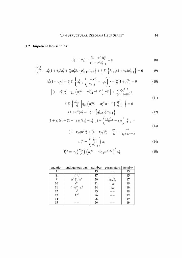
CAN STRUCTURAL REFORMS HELP SPAIN? 44
1.2 Impatient Households
λit(1+ τc)−
(1− aci)εzt
cit − acici
t−1= 0 (8)
ahiεht
hit− λi
t(1+ τh)qht + ξ i
tmitEt
{qh
t+1πt+1
}+ βiEt
{λi
t+1(1+ τh)qht+1
}= 0 (9)
λit(1− τ f b)− βiEt
{λi
t+1
(1+ rbi
tπt+1
− τ f b
)}− ξ i
t(1+ rbit ) = 0 (10)
[(1− ε`t )`
it − ηw
(πwi
t − πιw
t−1π1−ιw)
πwit
]+
a`iε`t `i1+φt
λit(1−τw)wi
t+
βiEt
{λi
t+1λi
t
[ηw
(πwi
t+1 − πιwt π1−ιw
)πwi2
t+1πt+1
]}= 0
(11)
(1+ rbi)bit = mi
tEt
{qh
t+1hitπt+1
}(12)
(1+ τc)cit + (1+ τh)qh
t (hit − hi
t−1) +
(1+rbi
t−1πt− τ f b
)bi
t−1 =
(1− τw)wit`
it + (1− τ f b)bi
t −Tui
tγi− Tg
t(γp+γi+γe)
(13)
πwit =
(wi
twi
t−1
)πt (14)
Tuit = γi
(ηw2
) (πwi
t − πιwt−1π1−ιw
)2wi
t (15)
equation endogenous var. number parameters number7 . . . 15 . . . 158 ci, λi 17 −− 159 hi, ξ i, mi 20 ahi, βi 17
10 rbi 21 τ f b 1811 `i, πwi, wi 24 a`i 1912 bi 25 −− 1913 Tui 26 −− 1914 −− 26 −− 1915 −− 26 −− 19

CAN STRUCTURAL REFORMS HELP SPAIN? 45
1.3 Hand-to-Mouth Households
(1−τw1+τc
) [(1− ε`t )`
mt − ηw
(πwm
t − πιw
t−1π1−ιw)
πwmt
]+
a`mε`t `m1+φt
Umc,tw
mt+
βmEt
{Um
c,t+1Um
c,t
[ηw
(1−τw1+τc
) (πwm
t+1 − πιwt π1−ιw
)πwm2
t+1πt+1
]}= 0
(16)
(1+ τc)cmt = (1− τw)wm
t `mt −
Tumt
γm(17)
Umc,t ≡
(1− acm)εzt
cmt − acmcm
t−1(18)
πwmt =
(wm
twm
t−1
)πt (19)
Tumt = γm
(ηw2
) (πwm
t − πιwt−1π1−ιw
)2wm
t (20)
equation endogenous var. number parameters number15 . . . 26 . . . 1916 `m, πwm, wm, Um
c 30 a`m, βm 2117 cm, Tum 32 γm 2218 −− 32 −− 2219 −− 32 −− 2220 −− 32 −− 22
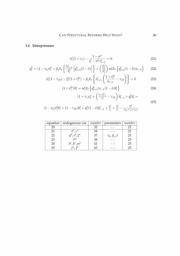
CAN STRUCTURAL REFORMS HELP SPAIN? 46
1.4 Entrepreneurs
λet(1+ τc)−
1− ace
cet − acece
t−1= 0 (21)
qkt = (1− τk)rk
t + βeEt
{λe
t+1λe
t
[qk
t+1(1− δ)]}+
(ξe
tλe
t
)me
t Et
{qk
t+1(1− δ)πt+1
}(22)
λet(1− τ f b)− ξe
t(1+ rbet )− βeEt
{λe
t+1
(1+ rbe
tπt+1
− τ f b
)}= 0 (23)
(1+ rbet )b
et = me
t Et
{qk
t+1πt+1(1− δ)ket
}(24)
(1+ τc)cet +
(1+rbe
t−1πt− τ f b
)be
t−1 + qkt ke
t =
(1− τk)rkt ke
t + (1− τ f b)bet + qk
t (1− δ)ket−1 +
Jxt
γe+
Jkt
γe− Tg
t(γp+γi+γe)
(25)
equation endogenous var. number parameters number20 . . . 32 . . . 2221 λe, ce 34 −− 2222 qk, rk, ξe 37 τk, βe, δ 2523 rbe 38 −− 2524 be, ke, me 41 −− 2525 Jx, Jk 43 −− 25

CAN STRUCTURAL REFORMS HELP SPAIN? 47
1.5 Intermediate goods producers
wpt =
µp(1− α)
xt
yxt
`ppt
(26)
wit =
µi(1− α)
xt
yxt`ii
t(27)
wmt =
µm(1− α)
xt
yxt
`mmt
(28)
ψ′(ut) =At
xt
(Kg
t−1γe
)αg
α
(`
ppt
)µp (`ii
t)µi(`mm
t )µm
keet−1ut
1−α
(29)
rkt = βeEt
{λe
t+1λe
t
[ψ′(ut+1)ut+1 − ψ(ut+1)
]}(30)
yxt = At
(kee
t−1ut)α[(`
ppt
)µp (`ii
t
)µi
(`mmt )µ
m]1−α
(Kg
t−1γe
)αg
(31)
Jxt
γx=
yxt
xt− wp
t `ppt − wi
t`iit − wm
t `mmt − rk
t keet − ψ(ut)kee
t−1 −Φx (32)
ψ(ut) ≡ ψu1(ut − 1) +
ψu2
2(ut − 1)2
equation endogenous var. number parameters number25 . . . 43 . . . 2526 x, yx, `pp 46 µp, α 2727 `ii 47 µi 2828 `mm 48 µm 2929 u, Kg, kee 51 ψu1
, αg, γx, 3230 −− 51 −− 3231 −− 51 −− 3232 −− 51 Φx 33

CAN STRUCTURAL REFORMS HELP SPAIN? 48
1.6 Capital producers and good retailers
qkt
[1− ηi
2
(itεk
tit−1− 1)2− ηi
(itεtk
it−1− 1)(
εkt
it−1
)it
]+
βeEt
{λe
t+1λe
t
[qk
t+1εkt+1ηi
(it+1εk
t+1it− 1)(
it+1it
)2]}
= 1
(33)
kt − (1− δ)kt−1 =
1− ηi2
(itε
kt
it−1− 1
)2 it (34)
Jkt
γk= qk
t
1− ηi
2
(itεk
tit−1− 1
)2 it
− it −Φk (35)
1− εyt +
εyt
xt− ηpπt
(πt − π
ιpt−1π
1−ιpss
)+
βpEt
{λ
pt+1λ
pt
[π2
t+1
(yt+1
yt
)ηp
(πt+1 − π
ιpt π
1−ιpss
)]}= 0
(36)
JRtγ= yt
[1− 1
xt−
ηp
2
(πt − π
ιpt−1π
1−ιpss
)2]
(37)
equation endogenous var. number parameters number32 . . . 51 . . . 3333 i, εk 53 ηi 3434 k 54 −− 3435 −− 54 −− 3436 εy 55 −− 3437 y 56 −− 34

CAN STRUCTURAL REFORMS HELP SPAIN? 49
1.7 Banks and monetary policy
(1+ rt) = (1+ rss)(1−φr)(1+ rt−1)
φr
(πt
π
)φπ(1−φr)(
yt
yt−1
)φy(1−φr)
(1+ ert) (38)
(rbt − rt) = −ηb
(kb
t
bbt− νb
)(kb
t
bbt
)2
(39)
πtkbt =
(1− δb
εkbt
)kb
t +ωb
(πt Jb
t−1γb
)(40)
bbt = db
t + kbt (41)
1+ rtrd
t
(θd
tθd
t−1
)−(
θdt
θdt−1
)+ ηp
(rd
trd
t−1− 1)
rdt
rdt−1
−βpEt
{λ
pt+1λ
pt
[ηp
(rd
t+1rd
t− 1)(
rdt+1rd
t
)2dpp
t+1dpp
t
]}= 0
(42)
dbt − dpp
t = 0 (43)
equation endogenous var. number parameters number37 . . . 56 . . . 3438 r 57 ηb, νb 3639 rb, kb, bb 60 δb, γb 3840 εkb, 61 −− 3841 db 62 −− 3842 θd 63 −− 3843 dpp 64 −− 38

CAN STRUCTURAL REFORMS HELP SPAIN? 50
1+ rbt
rbit
(θbi
tθbi
t −1
)−(
θbit
θbit −1
)− ηbi
(rbi
trbi
t−1− 1)
rbit
rbit−1
+βpEt
{λ
pt+1λ
pt
[ηbi
(rbi
t+1rbi
t− 1)(
rbit+1rbi
t
)2bii
t+1bii
t
]}= 0
(44)
1+ rbt
rbet
(θbe
tθbe
t −1
)−(
θbet
θbet −1
)− ηbe
(rbe
trbe
t−1− 1)
rbet
rbet−1
+βpEt
{λ
pt+1λ
pt
[ηbe
(rbe
t+1rbe
t− 1)(
rbet+1rbe
t
)2bee
t+1bee
t
]}= 0
(45)
bbt − bii
t − beet −
Bgt
γb= 0 (46)
jbt = rbi
t biit + rbe
t beet + θ
gssrb
t
(Bg
tγb
)− rd
t dppt −
ηb2
(kb
tbb
t− νb
)2kb
t
− ηd2
(rd
trd
t−1− 1)2
rdt dt − ηbi
2
(rbi
trbi
t−1− 1)2
rbit bii
t −ηbe2
(rbe
trbe
t−1− 1)2
rbet bee
t
(47)
equation endogenous var. number parameters number43 . . . 64 . . . 3844 bii, θbi 66 −− 3845 bee, θbe 68 −− 3846 Bg 69 −− 3847 θg 70 −− 38

CAN STRUCTURAL REFORMS HELP SPAIN? 51
1.8 Fiscal policy
Kgt = (1− δg)K
gt−1 + Ig
t (48)
ψbgt ≡
(Bg
tγyt
)(49)
ψcgt ≡
(Cg
tγyss
)(50)
ψig ≡(
Igt
γyss
)(51)
ψtg ≡(
Tgt
γyss
)(52)
ψcgt = (1− ρcg)ψ
cgss + ρcgψ
cgt−1 + σcgecg
t (53)
ψigt = (1− ρig)ψ
igss + ρigψ
igt−1 + σigeig
t (54)
ψtgt = ψ
tgt−1 + ρtg1
(ψbgt − ψ
bgss ) + ρtg2
(ψbgt − ψ
bgt−1) (55)
equation endogenous var. number parameters number47 . . . 70 . . . 3848 Ig, ψcg 72 δg 3949 ψbg 73 −− 3950 Cg, ψcg 75 −− 3951 ψig 76 −− 3952 Tg, ψig 78 −− 3953 −− 78 ρcg, σcg 4154 −− 78 ρig, σig 4355 −− 78 ρtg1, ρtg2 45

CAN STRUCTURAL REFORMS HELP SPAIN? 52
Cgt + Ig
t +
(1+ θ
gssrb
t−1πt
)Bg
t−1 = Bgt + Tg
t
+ τc
[γpcp
t + γicit + γece
t + γmcmt
]+ τhqh
t
[γp
(hp
t − hpt−1 )+γi( hi
t − hit−1
)]+ τw
[wp
t γp`pt + wi
tγi`it + wm
t γm`mt
]+ τkrk
t Kt
+ τ f b
[γp(d
pt − dp
t−1) + γi(bit − bi
t−1)) + γe(bet − be
t−1))]
+ τd
(rd
t−1πt
)γpdp
t−1 (56)
equation endogenous var. number parameters number55 . . . 78 . . . 4556 −− 78 −− 45
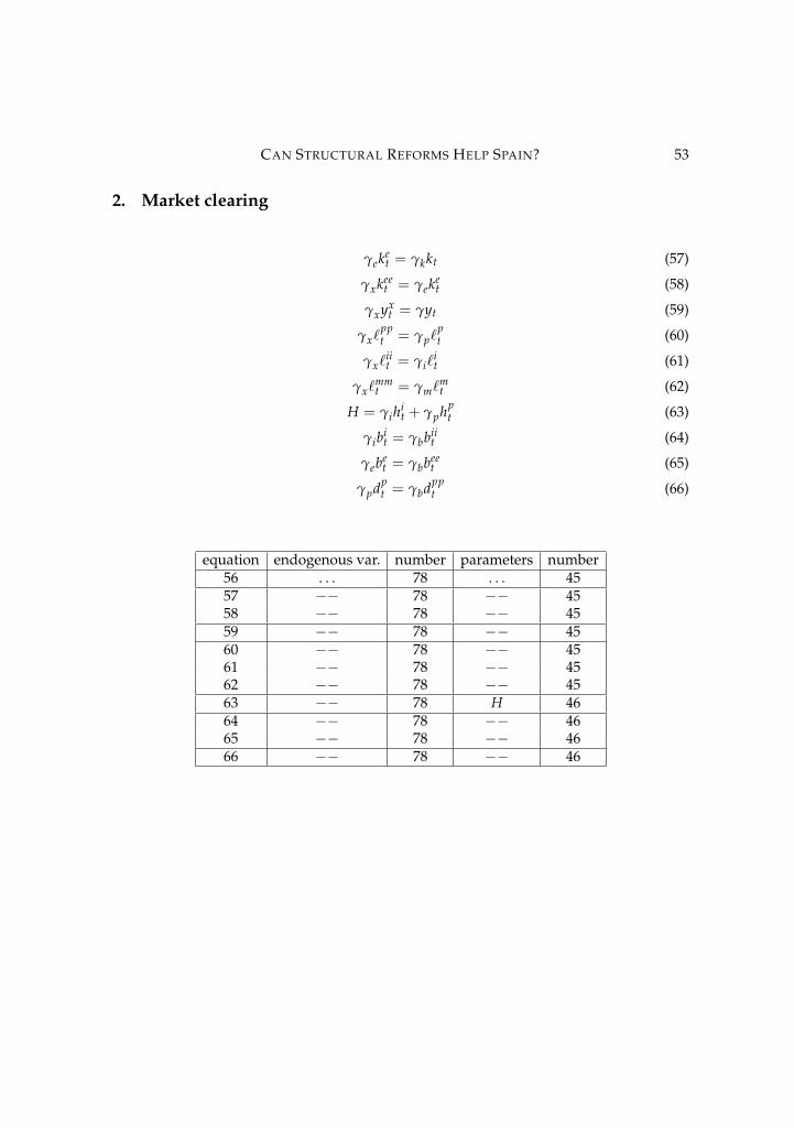
CAN STRUCTURAL REFORMS HELP SPAIN? 53
2. Market clearing
γeket = γkkt (57)
γxkeet = γeke
t (58)
γxyxt = γyt (59)
γx`ppt = γp`
pt (60)
γx`iit = γi`
it (61)
γx`mmt = γm`
mt (62)
H = γihit + γphp
t (63)
γibit = γbbii
t (64)
γebet = γbbee
t (65)
γpdpt = γbdpp
t (66)
equation endogenous var. number parameters number56 . . . 78 . . . 4557 −− 78 −− 4558 −− 78 −− 4559 −− 78 −− 4560 −− 78 −− 4561 −− 78 −− 4562 −− 78 −− 4563 −− 78 H 4664 −− 78 −− 4665 −− 78 −− 4666 −− 78 −− 46

CAN STRUCTURAL REFORMS HELP SPAIN? 54
3. Aggregation and equilibrium
Kt ≡ γkkt (67)
It = γkit (68)
Yt ≡ γyt (69)
Ct =[γpcp
t + γicit + γece
t + γmcmt
](70)
Bit ≡ γib
it (71)
Bet ≡ γebe
t (72)
Bt ≡ Bet + Bi
t + Bgt (73)
Kbt ≡ γbkb
t (74)
Dt ≡ γbdbt (75)
equation endogenous var. number parameters number66 . . . 78 . . . 4667 K 79 −− 4668 I 80 −− 4669 Y 81 −− 4670 C 82 −− 4671 Bi 83 −− 4672 Be 84 −− 4673 B 85 −− 4674 Kb 86 −− 4675 D 87 −− 46
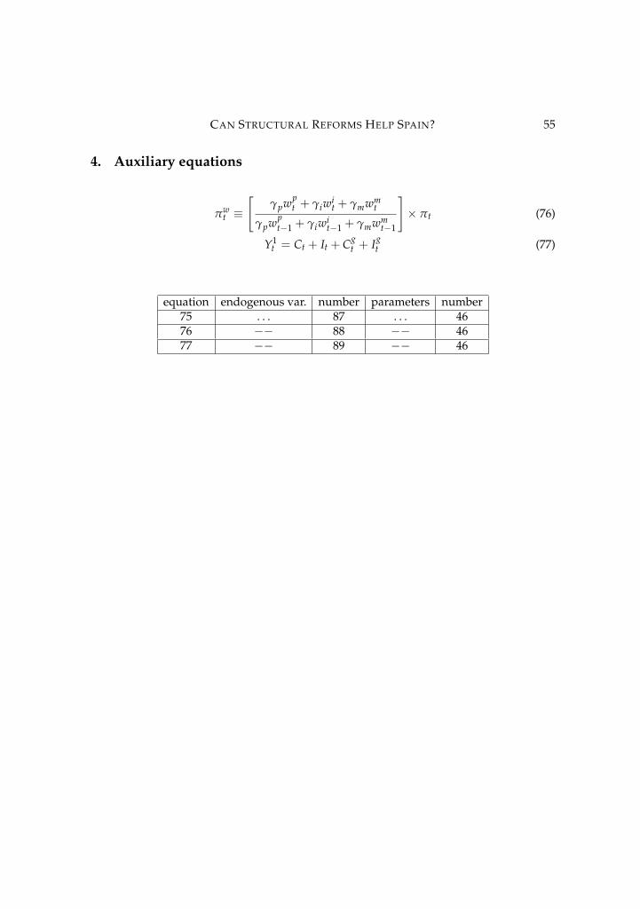
CAN STRUCTURAL REFORMS HELP SPAIN? 55
4. Auxiliary equations
πwt ≡
[γpwp
t + γiwit + γmwm
t
γpwpt−1 + γiwi
t−1 + γmwmt−1
]× πt (76)
Y1t = Ct + It + Cg
t + Igt (77)
equation endogenous var. number parameters number75 . . . 87 . . . 4676 −− 88 −− 4677 −− 89 −− 46
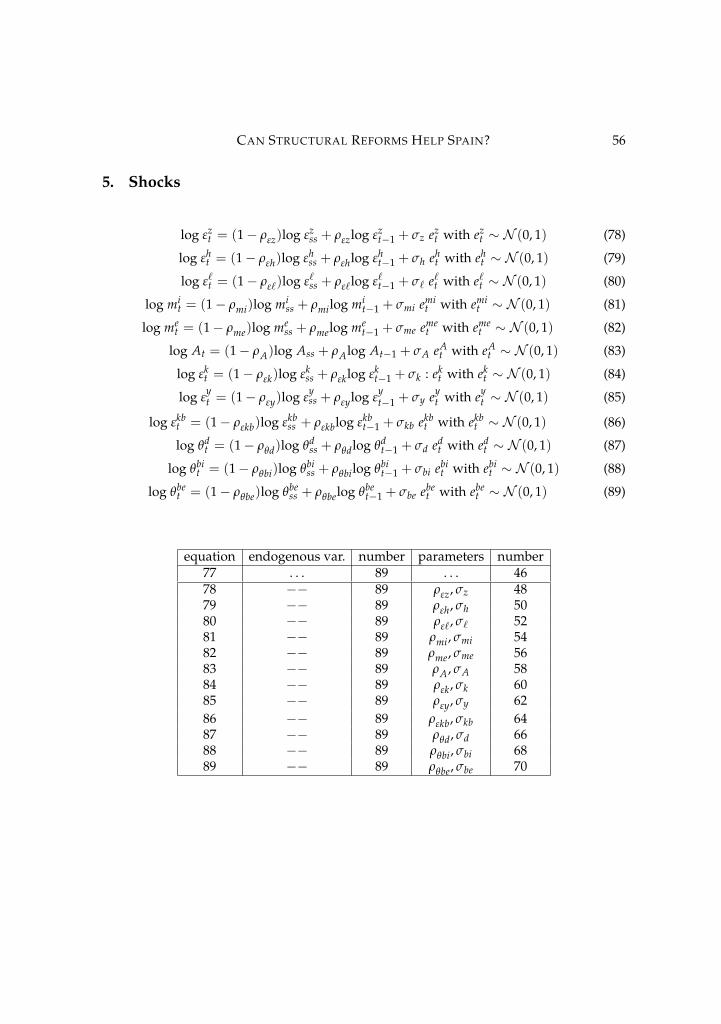
CAN STRUCTURAL REFORMS HELP SPAIN? 56
5. Shocks
log εzt = (1− ρεz)log εz
ss + ρεzlog εzt−1 + σz ez
t with ezt ∼ N (0, 1) (78)
log εht = (1− ρεh)log εh
ss + ρεhlog εht−1 + σh eh
t with eht ∼ N (0, 1) (79)
log ε`t = (1− ρε`)log ε`ss + ρε`log ε`t−1 + σ` e`t with e`t ∼ N (0, 1) (80)
log mit = (1− ρmi)log mi
ss + ρmilog mit−1 + σmi emi
t with emit ∼ N (0, 1) (81)
log met = (1− ρme)log me
ss + ρmelog met−1 + σme eme
t with emet ∼ N (0, 1) (82)
log At = (1− ρA)log Ass + ρAlog At−1 + σA eAt with eA
t ∼ N (0, 1) (83)
log εkt = (1− ρεk)log εk
ss + ρεklog εkt−1 + σk : ek
t with ekt ∼ N (0, 1) (84)
log εyt = (1− ρεy)log ε
yss + ρεylog ε
yt−1 + σy ey
t with eyt ∼ N (0, 1) (85)
log εkbt = (1− ρεkb)log εkb
ss + ρεkblog εkbt−1 + σkb ekb
t with ekbt ∼ N (0, 1) (86)
log θdt = (1− ρθd)log θd
ss + ρθdlog θdt−1 + σd ed
t with edt ∼ N (0, 1) (87)
log θbit = (1− ρθbi)log θbi
ss + ρθbilog θbit−1 + σbi ebi
t with ebit ∼ N (0, 1) (88)
log θbet = (1− ρθbe)log θbe
ss + ρθbelog θbet−1 + σbe ebe
t with ebet ∼ N (0, 1) (89)
equation endogenous var. number parameters number77 . . . 89 . . . 4678 −− 89 ρεz, σz 4879 −− 89 ρεh, σh 5080 −− 89 ρε`, σ` 5281 −− 89 ρmi, σmi 5482 −− 89 ρme, σme 5683 −− 89 ρA, σA 5884 −− 89 ρεk, σk 6085 −− 89 ρεy, σy 6286 −− 89 ρεkb, σkb 6487 −− 89 ρθd, σd 6688 −− 89 ρθbi, σbi 6889 −− 89 ρθbe, σbe 70

CAN STRUCTURAL REFORMS HELP SPAIN? 57
6. Total resources constraint
Yt = Ct + It + Cgt + Ig
t +[ψu1(ut − 1) +
ψu22 (ut − 1)2
]Kt−1 + δb
Kbt−1πt+
ηp2
(πt − π
ιpt−1π1−ιp
)2Yt
+ 1πt
[ηd2
(rd
t−1rd
t−2− 1)2
rpt−1Dt−1 +
ηi2
(rbi
t−1rbi
t−2− 1)2
rbit−1Bi
t−1 +ηe2
(rbe
trbe
t−2− 1)2
rbet−1Be
t−1
]
+ηb2
(Kb
t−1Bt−1− νb
)2Kb
t−1πt+
γpηw2
(π
wpt − πιw
t−1π1−ιw)2
wpt +
γiηw2(πwi
t − πιwt−1π1−ιw
)2 wit
+γmηw
2(πwm
t − πιwt−1π1−ιw
)2 wmt

CAN STRUCTURAL REFORMS HELP SPAIN? 58
ReferencesAndolfatto, D. (1996): "Business Cycles and Labor-Market Search", American Economic Review, 86 (1),
112–132.
Andrés, J. and O. Arce (2012): "Banking Competition, Housing Prices and Macroeconomic Stability",The Economic Journal, 122, 1346-1372.
Andrés, J., Boscá, J. E. and J. Ferri (2012): "Household Leverage and Fiscal Multipliers", Banco deEspaña Working Papers 1215, Banco de España.
Boscá, J. E., García, J. R. and D. Taguas (2005): "Effective Tax rates and Fiscal Convergence in theOECD: 1965-2001", Hacienda Pública Española, 174(3), 119-141.
Boscá, J.E., Doménech, R. and J. Ferri (2011): "Search, Nash Bargaining and Rule-of-Thumb Con-sumers", European Economic Review, 55(7), 927-942.
Calvo, G. (1983): "Staggered Pricing in a Utility Maximizing Framework", Journal of Monetary Eco-nomics, 12, 383-96.
Chéron, A. and F. Langot (2004): "Labor Market Search and Real Business Cycles: Reconciling NashBargaining with the Real Wage Dynamics", Review of Economic Dynamics, 7, 476-493.
Christiano, L., Eichenbaum, M. and S. Rebelo (2011) "When is the Government Spending MultiplierLarge?", Journal of Political Economy, 119, 78-121.
Choi, S. and J. V. Rios-Rull (2009): "Understanding the Dynamics of Labor Share: The Role of Non-competitive Factor Prices", Annales d’Economie et de Statistique, issue 95-96, 251-277.
Cloyne, J. and P. Surico (2014): "Household Debt and the Dynamic Effects of Income Tax Changes",Bank of England Working Paper No. 491, Bank of England.
Coenen, G., McAdam, P. and R. Straub (2008): "Tax Reform and Labour-Market Performance inthe Euro Area: A Simulation-Based Analysis Using the New Area-Wide Model", Journal ofEconomic Dynamics and Control, 32(8), 2543-2583..
Coenen, G., Erceg, C. J., Freedman, C., Furceri, D.; Kumhof, M., Lalonde, R., Laxton, D., Lindé, J.,Mourougane, A., Muir, D., Mursula, S., de Resende, C., Roberts, J., Roeger, W., Snudden,S., Trabandt, M. and in’t Veld, J. (2012): "Effects of Fiscal Stimulus in Structural Models",American Economic Journal: Macroeconomics, 4(1): 22–68.
Coenen, G., R. Straub and M. Trabandt (2013): "Gauging the Effects of Fiscal Stimulus Packages inthe Euro Area", Journal of Economic Dynamics and Control, 37, 367-386.
Cogan, J. F., Cwik, T., Taylor, J. B. and V. Wieland (2010): "New Keynesian versus old KeynesianGovernment Spending Multipliers", Journal of Economic Dynamics and Control, 34, 281-295
Cogan, J. F., Taylor, J. B., Wieland, W. and M. H. Wolters (2013): "Fiscal Consolidation Strategy",Journal of Economic Dynamics and Control, 37, 404–421.
Corsetti, G.,Kuester, K., Meier, A. and G. J. Müller (2010): "Debt Consolidation and Fiscal Stabiliza-tion of Deep Recessions", American Economic Review, 100(2), 41-45.
Davig, T. and E. M. Leeper (2011): "Monetary-fiscal policy interactions and fiscal stimulus", EuropeanEconomic Review, 55(2), 211-227.
Drautzburg, T. and H. Uhlig (2013): "Fiscal Stimulus and Distortionary Taxation", Working PaperNo. 13-46, Research Department. Federal Reserve Bank of Philadelphia.

CAN STRUCTURAL REFORMS HELP SPAIN? 59
ECB (2014): "Fiscal Multipliers and the Timing of Consolidation", ECB Monthly Bulletin, April, Euro-pean Central Bank, Frankfurt.
Eggertsson, G. B. (2011): "What Fiscal Policy is Effective at Zero Interest Rates?" NBER Macroeco-nomics Annual 2010, 25, ed. Daron Acemoglu and Michael Woodford, 59–112, University ofChicago Press.
Eggertsson, G. B. and P. Krugman (2012): "Debt, Deleveraging, and the Liquidity-Trap: A Fisher,Minsky, Koo Approach", Quarterly Journal of Economics, 127(3), 1469–1513.
Eggertsson, G. B., A. Ferrero and A. Raffo (2014): "Can Structural Reforms Help Europe?," Journal ofMonetary Economics, 61(C), 2-22.
Erceg, C. J. and J. Lindé (2011): "Asymmetric Shocks in a Currency Union with Monetary and FiscalHandcuffs", NBER International Seminar on Macroeconomics, 7(1), 95-136.
Erceg, C. J. and J. Lindé (2013): "Fiscal Consolidation in a Currency Union: Spending Cuts vs. TaxHikes", Journal of Economic Dynamics and Control, 37, 422-445.
Faia, E., Lechthaler, W.; and C. Merkl (2010): "Fiscal Multipliers and the Labour Market in the OpenEconomy" IZA Discussion Papers 4849, Institute for the Study of Labor (IZA).
Farhi, E. and I. Werning (2012): "Fiscal Multipliers: Liquidity Traps and Currency Unions", NBERWorking Papers 18381.
Forni, L., Monteforte, L. and L. Sessa (2009): "The General Equilibrium Effects of Fiscal Policy: Esti-mates for the Euro Area", Journal of Public Economics, 93, 559–585.
Gadatsch, N., Hauzenberger, K. and N. Stähler (2014): "Getting into GEAR: German and the Rest ofEuro Area Fiscal Policy During the Crisis", mimeo, Bundesbank, Frankfurt.
Galí, J. (2011): "The Return Of The Wage Phillips Curve," Journal of the European Economic Association,9(3), 436-461.
Galí, J. (2013): "Notes for a New Guide to Keynes (I): Wages, Aggregate Demand, and Employment."Journal of the European Economic Association, 11(5), 973-1003. http://goo.gl/Jjz2ns