erlang – c formula - tripod.comigorcekicevski.tripod.com/import/derivatives.pdf · we have...
TRANSCRIPT

COM DEPARTMENT
34340
TELETRAFFIC ENGINEERING ANDNETWORK PLANNING
ERLANG – C FORMULA
VILLY BÆK IVERSEN, PH.DIGOR CEKICEVSKI, M.SC.E.E
LyngbyMay 15th, 2004
TECHNICAL UNIVERSITY OF DENMARK INTERNATIONAL MASTER OF SCIENCE PROGRAM

Teletraffic Engineering and Network Planing Erlang – C Formula
Contents
Abstract…………………………………………………………………………………………………………………………………………...…3
1. Introduction………………………..………………………………………………………………………………………………………….4
2. Queuing Theory and Erlang - C Formula………..…………………………………………………………………...…….62.1 Derivation of Erlang – C Formula…..…………………………………………………………………………………...72.2. Calculation of the Carried and Offered Traffic………..…………………………………………….…………...92.3 Various Representations of Erlang – C……………………………………………………………….………….….10
2.3.1 Relation between Erlang – C and Erlang –B……………………………………………………..…..102.3.2 Tabular Representation…….…………………………………………………………………………………….112.3.3 Graphical Interpretation…………………………………………………………………………………...….…112.3.4 MATLAB Code for Erlang – C......................................................................................................................12 2.3.5 Recursive Erlang – C formula and its inversion…………………..……………………..………….132.3.6 MATLAB Code for Inverse Erlang – C........................……………………………...…………142.3.7 Sander’s Formula...................…………………….......…………………………………..……………...…………15
3. Queue Length Distribution (QLD) ........................…………………………………………………………...…...…………16 3.1 MATLAB Code for PDF and QLD – M/M/n........................………………………………….....…...…………17 3.2 Mean Queue Length........................……………………………………………………………...…...……………….………18
3.2.1 Mean Queue Length at an arbitrary point of time.........................…………………………………18 3.2.2 Mean Queue Length, if the queue is greater than zero...…....................……………………...…19
4. Waiting Time Distribution (WTD) - M/M/n........................……………….……………………………………………21 4.1 Waiting Time Distribution for M/M/n, FCFS........................………………………………………………....…21 4.2 MATLAB Code for PDF and WTD – M/M/n........................……………….…………………...…...…………23 4.3 Waiting Time Distributions for other Queuing Disciplines....…...…………………………....……..……24 4.4 Mean Waiting Time........................…..………………………………………………………...…...………………...………25
4.4.1 Mean Waiting Time - All customers...................………………….…...……………………....…………25 4.4.2 Mean Waiting Time - Delayed customers........................……………………...…………………...…25
5 Improvement Functions for M/M/n......................……………………………………………………………………….....…26 5.1 MATLAB Code for Improvement Function of M/M/n........................……..………………………...….…28
6. Finite-buffer Queuing System......................……..……………………………………………………………..………...…...…29 6.1. General considerations........................……..………………………...…..........................................................................…29
6.1.1 Single-server System........................……..………………………...……..........................................................…29 6.1.1.1 M/M/1/k........................……..……………………......................................................................…...…...…29
6.1.1.1.1. MATLAB Code for Blocking Probability in M/M/1/k......…...…..…30 6.1.1.2 M/G/1/k........................……..…………………......................................................................…........…...…31 6.1.1.3 M/D/1/k........................……..…………………….......................................................................…...…...…32
6.2. Multiple-server System........................……..……………………......................................................................…...…...…32 6.2.1 Steady State Probabilities.......................……..…………………….......................................................………32 6.2.2 Blocking Probability – M/M/n/k........................……..………..………………...............................….……33
6.2.2.1 MATLAB Code for the Blocking Probability in M/M/n/k......................……....…33 6.2.3 Queue Length Distribution – M/M/n/k......................….……………………………………………...…35
6.2.3.1. MATLAB Code for PDF and QLD – M/M/n/k......................….…………………...…35
2

Teletraffic Engineering and Network Planing Erlang – C Formula
6.2.3.2 Mean Queue Length – M/M/n/k......................….……………………………………..……..…37 6.2.4 Waiting Time Distribution – M/M/n/k......................….…………….…...……………...……..……..…38
6.2.4.1 Mean Waiting Time – M/M/n/k......................….…………………………………...………..…39
7. Cost Function....................….………………………………….………………………………………………………………………..…40
8. Priority of customers......................….………………………………………………………………………………………….…..…41 8.1 Analysis of M/M/n/K Queues with Priorities......................….……………………...………….……………..…42
8.1.1 M/M/-/- Queue with Pre-emptive Priority......................….………………………………….……..…42 8.1.1.1 Mean Waiting Time for Pre-emptive-resume Queuing Discipline...…...…..…45 8.1.1.2 Mean Queue Length for Pre-emptive-resume Queuing Discipline................…46
8.1.2 M/M/-/- Queue with Non-pre-emptive Priority......................….…………………………..…..…46 8.1.2.1 Mean Waiting Time for Non-pre-emptive Queuing Discipline (M/M/n).…48 8.1.2.2 Mean Queue Length for non-pre-emptive Queuing Discipline (M/M/n).....49
8.2 Concrete example for a Non-pre-emptive Priority System……………………..…………………....…....49 8.2.1 Disks in SAN……………………………………………………………………………………………………….....50
8.2.1.1 Read and Write Requests…………………………………………………………………………...508.2.1.2 Disk Response Time………………………………………………………………………………......51
8.3 Analysis Model………………………………………………………………………………………………………………......518.3.1 Basic Assumptions………………………………………………………………………………………………....518.3.2 Finite Queuing Model………………………………………………………………………………………….....52
8.3.2.1 State Probabilities……………………………………………………………………………………....528.3.2.2 Performance Measures…………………………………………………………………………….....528.3.2.3 Numerical Results………………………………………………………………………………...…....53
9. Systems with Limited Waiting Time………………………………………..……………………………………….……....549.1 Exponentially distributed Time-out Interval……………..…………………………………………………….....54 9.2 Systems with Constant Time-out Interval……………………………………..…………………………………...549.2.1. State Probabilities– Systems with Constant Time-out Interval…………………….…….………....55
9.2.2 Queue Length Distribution – Systems with Constant Time-out Interval……..………..55 9.2.2.1 Mean Queue Length - Systems with Constant Time-out Interval……..……....56
9.2.3. Waiting Time Distribution - Systems with Constant Time-out Interval……..…..…....569.2.3.1 MATLAB Code for PDF and WTD of Systems with Constant Time-out Interval……..…………………………………...…………………………………………………………....58 9.2.3.2. Mean Waiting Time - Systems with Constant Time-out Interval……..…......59
10. Concluding remarks……..……………………………………………………………………………………...…………………....60
Appendix A – Gamma Function.……..……………………………………………………………………………………….…....61
Appendix B – Error Function……..………………………………………………………………………………………………....62
Glossary of Acronyms…….……………………………………………………………………………………………………………....63
References……..………………………………………………………………………………………………………………………………....64
3

Teletraffic Engineering and Network Planing Erlang – C Formula
Abstract
This paper deals with the queuing systems in different configurations. As the basic tool dealing with problems, related to these systems, we put our emphasis to Erlang - C formula. It denotes by what probability an arbitrary customer arriving to the queuing system would experience waiting i.e delay before service is performed. Since its pure form is not adequate in computer simulation processes we have derived it in terms of Erlang - B formula. There are also other forms that we have considered, such as Erlang - C recursive formula and Erlang - C inverse formula.
The remaining part of the paper concentrates on waiting time and length distributions in queuing systems with infinite and finite buffer. Finite queues are often hard or impossible to analyse in an exact analytical way. In such cases, the often-preferred solution is to approximate the loss probability in a finite queue by the probability that the corresponding infinite queue (with the same service time) exceeds the finite queue length. We confirm the theoretical results with the appropriate MATLAB codes, together with corresponding graphical representations.
4

Teletraffic Engineering and Network Planing Erlang – C Formula
1. Introduction
Queuing theory is the mathematical study of waiting. It is concerned with the mathematical modeling and analysis of systems that provide service to random demand. Queuing theory has played an important role in modeling communications networks. The generic procedure is to model a system as a stochastic queuing system or a random process. A (single) queuing system has three components: customers, one or multiple servers, and a single queue, and involves two processes i.e. the arrival process and the service process. Customers arrive at the system and get service from the server(s). If all the servers are busy in serving other customers, a newly arriving customer will wait in the queue until a server becomes idle, hence the name queuing systems. In this report, the queue refers to a queuing system as well as to a buffer. The key random processes used in queuing theory are Markov processes.
There are several everyday examples that can be described as queuing systems, such as bank-teller service, computer systems, manufacturing systems, maintenance systems, communications systems, and etc.A queuing system is characterized by the following three components:
• Arrival process • Service mechanism• Queue discipline
Arrival processes. Arrival processes, such as telephone calls arriving to an exchange are described mathematically as stochastic point processes. We can define two basic arrival processes:
• Point process. It is the case when any two arrivals must be distinguished from each other. Information concerning the single arrival (e.g. service time, number of customers) is ignored. Such information can only be used to determine whether an arrival belongs to the process or not. For telephone calls this may be realized by choosing sufficient detailed time scale. We always assume Poisson arrival process.
• Multiple arrivals. It is the case when at the input of the server there are two or more arrivals at the same time. This is more complex situation then the previous one and therefore it is no considered in this report.
Service mechanism. There are many service mechanisms. In order to describe them we need to know the number of servers in the system and the average duration of the service time. The number of servers can vary from one to infinity. On the other hand the distribution of the service time can be divided into two main groups:
• General • Deterministic
5

Teletraffic Engineering and Network Planing Erlang – C Formula
Queue Discipline. Discipline of a queuing system defines the rule that is used by a server when it chooses the next customer from the queue (if any) when the service of the current customer is completed. Commonly used queue disciplines are:
• FIFO. Customers are served on a First – In – First - Out basis • LIFO. Customers are served in Last – In – First - Out manner • Priority. Customers are served in order of their importance on the basis of their service
requirements.
Erlang-C is most commonly used to calculate how long calls will have to wait before the connection to the destination is established. This model assumes that all blocked calls stay in the system until they are handled. Also, it can be applied to the design of call-canter staffing arrangements where, if calls cannot be immediately answered, they enter a queue.
Erlang-C formula is only valid for Poisson arrival process and an exponential holding time distribution. It denotes what the possibility is that an arbitrary customer arriving to the queuing system would experience waiting i.e. delay before service is performed. Erlang–C is much similar to Erlang–B. However the major difference is that Erlang–B applies to loss systems.
6

Teletraffic Engineering and Network Planing Erlang – C Formula
2. Queuing Theory and Erlang - C formula
A queue is a waiting line (like customers waiting at a supermarket checkout counter) and queuing theory is the mathematical theory of waiting lines. More generally, queuing theory is concerned with the mathematical modelling and analysis of systems that provide service to random demands. A queuing model is an abstract description of such a system. Typically, a queuing model represents:
• The physical configuration of the system, by specifying the number and arrangement of the servers, that provide service to the customers
• The stochastic (i.e probabilistic or statistical) nature of the demands, by specifying the variability in the arrival process and in the service process.
For instance, in computer communications, a communication channel might be a server, and messages could represent customers. The (random) time at which messages request the use of the channel would be the arrival process, and the (random) duration of service time for the messages while being transmitted would constitute the service process.
Queuing theory was born in the early 1900s with the work of A. K. Erlang at the Copenhagen Telephone Company, who derived several important formulae for teletraffic engineering that today bear his name. The range of applications has grown and today they cover not only telecommunications and computer science, but also manufacturing, air traffic control, military logistics, and many other areas that involve service systems whose demands are random.
The essence of queuing theory is that it takes into account the randomness of the arrival process and the randomness of the service process. The most common assumption about the arrival process is that the customer arrival epochs follow a Poisson process. One of the most important queuing models is the Erlang loss model. It assumes that the arrivals follow a Poisson process, and that the blocked customers (those who find all servers busy) are cleared i.e. they are denied entry into the system and therefore the blocked customers are lost. The fraction of arriving customers who find all servers busy (the probability of blocking, or loss probability) is given by the famous Erlang loss (or Erlang - B) formula.
The Erlang delay model (also called M/M/n in queuing theory) is similar to the Erlang loss model, except that now it is assumed that the blocked customers will wait in a queue as long as it is necessary for a server to become available. In this model, the probability of blocking (the fraction of customers who will find all n servers busy and must wait in the queue) is given by the famous Erlang delay (or Erlang C) formula.
7

Teletraffic Engineering and Network Planing Erlang – C Formula
2.1 Derivation of Erlang - C formula
In this section we consider a traffic that enters a system with n identical servers. Also we assume full accessibility and an infinite number of waiting positions in the buffer. If a customer arrives and sees all n servers busy then he joins a queue and waits until one server becomes idle. There is no option for a customer to be in the queue when a server is idle. This characteristic of the system is called full accessibility.
We shall consider the case of Poisson arrival process (an infinite number of sources) and exponentially distributed service times (PCT-I). This is the most important queuing system, called Erlang delay system. This system is denoted as M/M/n where the carried traffic is equal to the offered traffic since no customers are blocked.
Here, M stands for Poisson arrival process, whereas M for exponential service times and n designates the number of servers. Initially we shall assume a buffer with an infinite number of waiting positions. The probability of a positive waiting time, mean queue lengths, mean-waiting times, carried traffic per channel, and improvement functions will be dealt later in this report.
Figure 2.1 State transition diagram of the M/M/n Delay System having n servers and an unlimited number of waiting positions.
The state of the system is defined as the total number of customers in the system (either being served or waiting in queue). We are interested in the steady state probabilities of the system. The procedure begins with setting up the state transition diagram shown in Fig. 2.1. Assuming statistical equilibrium, the cut equations become:
)1()0( pp ⋅=⋅ µλ (2.1) )1(2)0( pp ⋅=⋅ µλ (2.2)
. .
. .
)1()1()( +⋅+=⋅ ipiip µλ (2.3). .. .
)()1( npnnp ⋅=−⋅ µλ (2.4)
8

Teletraffic Engineering and Network Planing Erlang – C Formula
)1()( +⋅=⋅ npnnp µλ (2.5). .. .
)1()( ++⋅=+⋅ jnpnjnp µλ (2.6)
λ represents the arrival intensity and 1/ µ is the mean service time. As A = λ /µ is the offered traffic, we get:
By normalization of the state probabilities we obtain p (0):
1)(0
=∑∞
=iip (2.8)
1...1!
...!21
1)0( 2
22
=
+++++++
nA
nA
nAAAp
n
(2.9)
Realizing the geometric progression with quotient A/n, the normalization condition can only be fulfilled for:
A < n (2.10)
Statistical equilibrium is only obtained for A < n. Otherwise, the queue will continue to increase towards infinity. We obtain:
∑−
= −+
=1
0 !!
1)0(n
i
ni
Ann
nA
iA
p , A ≤ n (2.11)
Equations (2.7) and (2.11) produce the steady state probabilities.
≥⋅
≤≤
−+
=
−
−
=∑ ni
nnA
niiA
Ann
nA
iA
ip
ni
i
i
n
i
ni
,!
0,!
!!
1)(1
0
, A ≤ n (2.12)
In the case when the Poisson arrival process is independent of the state of the system, the probability that an arbitrary arriving customer has to wait in the queue is equal to the proportion of
9
≥⋅
⋅=
⋅
≤≤⋅=
−
−
ninnAp
nAnp
niiAp
ip
ni
ini
i
,!
)0()(
0,!
)0()( (2.7)

Teletraffic Engineering and Network Planing Erlang – C Formula
time all servers are occupied (PASTA–property: Poisson Arrivals See Time Average). The waiting time is a random variable denoted by W. For an arbitrary arriving customer we have:
{ }0)(,2 >= WpAE n (2.13)
∑∑
∑ ∞
=∞
=
∞
= ==ni
i
nin ip
ip
ipAE )(
)(
)()(
0
,2
λ
λ (2.14)
AnnnpAE n −
= )()(,2 (2.15)
Finally, we can formulate the Erlang - C formula
Ann
nA
nA
nAAA
Ann
nA
E nnn
n
n
−+
−+
−++++
−= −
!)!1()!1(...
!211
!12,2 , A<n (2.16)
This delay probability depends only upon A, the product of λ and 1/µ, and not upon the parameters individually. According to the Erlang-C formula, the probability that a customer is served immediately upon arrival to the system is given by:
)(1 ,2 AES nn −= (2.17)
2.2 Calculation of the Carried and the Offered traffic
Since we are dealing with delay and lossless systems, it is intuitively that the carried and the offered traffic should coincide, as no customers are rejected and the arrival process is a Poisson process. The proof is given below. The carried traffic is given by
∑ ∑=
∞
+=
⋅+⋅=n
i niipnipiY
1 1
)()( (2.18)
Using the cut equations, we can reformulate (2.18) to obtain:
AipipYn
i ni==−⋅+−= ∑ ∑
=
∞
+= µλ
µλ
µλ
1 1
)1()1( (2.19)
10

Teletraffic Engineering and Network Planing Erlang – C Formula
2.3 Various Representations of Erlang - C
Erlang – C formula could be expressed in a number of different ways. This is crucial since it the direct evaluation of (2.16) seems to be very difficult. Some of these representations are analyzed in more detail below.
2.3.1 Relation between Erlang – C and Erlang –B
Knowing that Erlang – B formula (denoted by E1,n (A)) is given by
!)!1()!1(...
!211
!)( 12,1
nA
nA
nAAAnA
AE nnn
n
n
+−
+−
++++= − (2.20)
we can derive Erlang - C formula in order so that it is expressed in terms of Erlang – B formula. The whole procedure is explained below.
[ ]n
AEAAE
AEAnAEn
nAA
nA
An
nAAn
An
AE
iAA
iAn
nnA
nnA
iAAn
nnA
Ann
nA
iA
Ann
nA
AE
n
n
n
n
n
n
n
n
n
n
i
in
i
i
n
nn
i
i
n
nn
i
i
n
n
)(11
)())(1(
)(
!1
!1
!1
1!
)(
!!
!
!!)(
!
!!
!)(
,1
,1
,1
,1,2
1
00
1
0
1
0
,2
−⋅−
=−⋅−
⋅=
+⋅⋅⋅++−⋅−
+⋅⋅⋅++⋅
=
−=
+−=
−+
−⋅
=
∑∑∑∑−
==
−
=
−
=
( ) ( ) nAEAAE
AEAnAEn
AEn
n
n
nn /)(11
)()(1
)()(
,1
,1
,1
,1,2 −−
=−−
⋅= , A<n (2.22)
It is easily noticeable that:
)()( ,1,2 AEAE nn > (2.23)
as the term A[1 − E1,n(A)] /n is the average carried traffic per channel in the corresponding loss system. For nA ≥ , we have E2,n(A) = 1 since it is a probability and all customers are delayed.
11
(2.21)

Teletraffic Engineering and Network Planing Erlang – C Formula
2.3.2 Tabular Representation
Erlang - C formula has been tabulated in Moe’s Principle [2]. The Table 2.1 below denotes the value of the Erlang-C as a function of the offered traffic and the total number of servers.
Number of Servers
Table 2.1. Tabular representation of Erlang - C
2.3.3 Graphical Interpretation
Erlang – C can be also represented graphically. It is shown on Fig. 2.2.
Figure 2.2 Graphical interpretation of Erlang – C
12
Teletraffic Engineering and Network Planing Erlang – C Formula
2.3.4 MATLAB Code for Erlang C
function B = erlangb (n, A)% This function computes the Erlang B probability that a system with n% servers, no waiting line, Poisson arrival rate lambda, service rate % (per server) mu, and intensity A = lambda / mu will have all servers busy. % The probability is B=(A^m / m!) / (sum (A^k / k!), k=0…m)% The recurrence is B (0, A) = 1.% B (n, A)=(A*B (n - 1, A) / n) / (1+A*B (n - 1, A) / n) if ( (floor (n) ~= n) | (n < 1) ) warning ('n is not a positive integer'); A=NaN; return; end; if (A < 0.0) warning ('A is negative!'); A=NaN; return; end;B=1; for k=1:n, B=( (A*B) / k) / (1 + A*B / k); end;
function C=erlangc (n, A)% This function computes the Erlang C probability that a system with n% servers, infinite waiting line, Poisson arrival rate lambda, service rate % (per server) mu, and intensity A=lambda / mu will have all servers busy. % It uses the formula C (n, A)=n*B (n, A) / (n-A*(1 - B (n, A) ) ) if ( (floor (n) ~= n) | (n < 1) ) warning ('n is not a positive integer'); A=NaN; return; end; if (A < 0.0) warning ('A is negative!'); A=NaN; return; end;B=erlangb (n, A);C=n*B / (n - A*(1 - B) );
2.3.5 Recursive Erlang-C Formula and Its Inversion
13

Teletraffic Engineering and Network Planing Erlang – C Formula
Another expression for Erlang – C formula can be obtained in terms of its recursion. The appropriate derivation begins with its inverse representation (2.27). This form is also known as Sander’s formula, which will be also derived in section 2.3.7.
))(1()(
)(,1
,1,2 AEAn
AEnAE
n
nn −⋅−
⋅= (2.24)
nAEAAEnA
AEn
nn −⋅
⋅−=
)()()(
)(,2
,2,1 (2.25)
)1()()())1((
)(1,2
1,21,1 −−⋅
⋅−−=
−
−− nAEA
AEnAAE
n
nn (2.26)
)(1
)(1
)(1
1,1,1,2 AEAEAE nnn −
−= (2.27)
)())1(()1()(
)()()(
)(1
1,2
1,2
,2
,2
,2 AEnAnAEA
AEnAnAEA
AE n
n
n
n
n −
−
⋅−−−−⋅
−⋅−
−⋅= (2.28)
[ ] [ ] [ ] [ ][ ] [ ])())1(()()(
)()()1()()())1(()()(
1
1,2,2
,21,21,2,2
,2 AEnAAEnAAEnAnAEAAEnAnAEA
AE nn
nnnn
n −
−−
⋅−−⋅⋅−⋅−⋅−−⋅−⋅−−⋅−⋅
= (2.29)
[ ] [ ]{ } [ ][ ] [ ])())1(()()(
)())1(()1()()()())1(()()(
1
1,2,2
1,21,21,2,2
,2 AEnAAEnAAEnAnnAEAnAAEnAAAE
AE nn
nnnn
n −
−−−
⋅−−⋅⋅−⋅−−−−−⋅⋅−−⋅−−⋅⋅
= (2.30)
[ ] [ ] =⋅−−+⋅−−⋅− −− )())1(()())1(()( 1,21,2 AEnAnAEnAnA nn
[ ] [ ]{ })1()()()())1(()( 1,21,2,2 −−⋅⋅−−⋅−−⋅⋅= −− nAEAnAAEnAAAE nnn (2.31)
[ ] [ ][ ] [ ]{ })1()()()())1((
)())1(()())1(()()(
1,21,2
1,21,2,2 −−⋅⋅−−⋅−−⋅
⋅−−+⋅−−⋅−=
−−
−−
nAEAnAAEnAAAEnAnAEnAnA
AEnn
nnn (2.32)
[ ][ ] [ ]{ })1()()()())1((
)())1(()(
1,21,2
1,2,2 −−⋅⋅−−⋅−−⋅
⋅−−⋅=
−−
−
nAEAnAAEnAAAEnAA
AEnn
nn (2.33)
For n>>1, we obtain the following simplified expression:
14

Teletraffic Engineering and Network Planing Erlang – C Formula
)()( 1,2,2 AEnAAE nn −=
(2.34)
2.3.6 MATLAB Code for Inverse Erlang - C
function InvB=erlangbinv (n, A)% This function computes the Inverse Erlang B probability that a system with n% servers, no waiting line, Poisson arrival rate lambda, service rate % (per server) mu, and intensity A=lambda / mu will have all servers busy. % The inverse probability is InvB = 1 + (1 / A)*InvB (n - 1, A)% The recurrence is InvB (0, A) = 1% InvB (n, A) = 1 + (1 / A)*InvB (n - 1, A) if ( (floor (n) ~= n) | (n < 1) ) warning ('n is not a positive integer'); A=NaN; return; end; if (A < 0.0) warning ('A is negative!'); A=NaN; return; end;InvB=1; for k=1:n, InvB=1 + (1/A)*InvB (n-1, A); end;
function InvC=erlangcinv (n, A)% This function computes the inverse Erlang C probability that a system with n% servers, infinite waiting line, Poisson arrival rate lambda, service rate % (per server) mu, and intensity rho=lambda / mu will have all servers busy. % It uses the formula InvC (n, A) = InvB (n, A) – InvB (n - 1, A) if ( (floor (n) ~= n) | (n < 1) ) warning ('n is not a positive integer'); A=NaN; return; end; if (A < 0.0) warning ('A is negative!'); A=NaN; return; end;InvB=erlangbinv (n, A);InvC (n, A) = InvB (n, A) – InvB (n - 1, A);2.3.7 Sander’s Formula
As it can be noticed this formula gives the inverse expression of Erlang – C in terms of Erlang – B. and it is by far the most accurate one.
15

Teletraffic Engineering and Network Planing Erlang – C Formula
)(1
)(1
)(1
1,1,1,2 AEAEAE nnn −
−= (2.35)
The derivation procedure starts as follows:
[ ])(11
)()(
,1
,1,2
AEnA
AnEAE
n
nn
−−=
(2.36)
[ ] [ ])()(1
)(1
)()(1
)(1
,1
,1
,1,1
,1
,2 AEnAEA
AEAEnAEAn
AE n
n
nn
n
n ⋅−
−=⋅
−⋅−= (2.37)
Using the recursion formula for evaluation of Erlang - B the second term in (2.37) can be expressed by E1,n-1 (A).
)()(
)(1,1
1,1,1 AEAn
AEAAE
n
nn
−
−
⋅+⋅
= (2.38)
Now we may apply (2.38) to obtain the Sander’s formula for evaluating the Erlang - C formula.
)()(
)()(
1
)(1
)(1
1,1
1,1
1,1
1,1
,1,2
AEAnAEA
n
AEAnAEA
A
AEAE
n
n
n
n
nn
−
−
−
−
⋅+⋅
⋅
⋅+
⋅−⋅
−= (2.39)
)(1
)(1
)(1
1,1,1,2 AEAEAE nnn −
−= (2.40)
3. Queue Length Distribution (QLD) – M/M/n
16

Teletraffic Engineering and Network Planing Erlang – C Formula
The queue length distribution (QLD) is determined by the probabilities of observing the queuing system in the steady states p(n+1), p(n+2) etc i.e. the probability of having one, two etc. customers in the queue. Thus, the respective probability density function (PDF) is discrete.
)...1()2()()1()( ++++= LnpLnpLpS δδ (3.1)
The steady state probabilities have already been derived in section 2. The first few values of importance are:
)()1( npnAnp =+ (3.2)
)()1()2(2
npnAnp
nAnp
=+=+ (3.3)
An arbitrary steady state probability becomes:
)()1()( npnAinp
nAinp
i
=−+=+ (3.4)
Therefore, we find the following expression for PDF of QLD:
...)(...)1()()()()(2
+
+++
+= np
nALnp
nALnp
nALp
i
S δδ (3.5)
++
+++= ....)2()1()()()(
2
LnAL
nAL
nAnpLpS δδδ (3.6)
In terms of Erlang-C formula, (3.6) can be expressed by:
+
++
+−
−= ...)1()()()(
32
nAL
nAL
nA
nAn
AnnnpLpS δδ (3.7)
+
++
+−= ...)1()()()()(
32
,2 nAL
nAL
nA
nAnAELp nS δδ (3.8)
We can now proceed towards determining an expression for QLD. The probability of having customers in queue at a random point of time is denoted by:
17
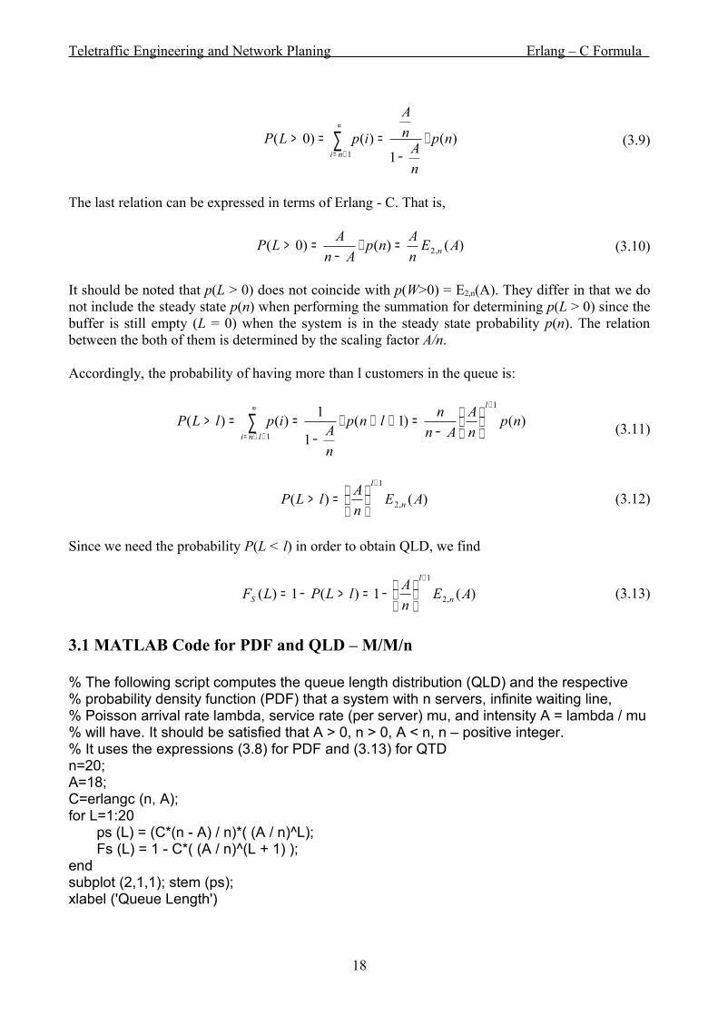
Teletraffic Engineering and Network Planing Erlang – C Formula
)(1
)()0(1
np
nA
nA
ipLPni
⋅−
==> ∑∞
+= (3.9)
The last relation can be expressed in terms of Erlang - C. That is,
)()()0( ,2 AEnAnp
AnALP n=⋅−
=> (3.10)
It should be noted that p(L > 0) does not coincide with p(W>0) = E2,n(A). They differ in that we do not include the steady state p(n) when performing the summation for determining p(L > 0) since the buffer is still empty (L = 0) when the system is in the steady state probability p(n). The relation between the both of them is determined by the scaling factor A/n.
Accordingly, the probability of having more than l customers in the queue is:
)()1(1
1)()(1
1
npnA
Annlnp
nA
iplLPl
lni
+∞
++=
−=++⋅
−==> ∑ (3.11)
)()( ,2
1
AEnAlLP n
l +
=> (3.12)
Since we need the probability P(L < l) in order to obtain QLD, we find
)(1)(1)( ,2
1
AEnAlLPLF n
l
S
+
−=>−= (3.13)
3.1 MATLAB Code for PDF and QLD – M/M/n
% The following script computes the queue length distribution (QLD) and the respective % probability density function (PDF) that a system with n servers, infinite waiting line, % Poisson arrival rate lambda, service rate (per server) mu, and intensity A = lambda / mu% will have. It should be satisfied that A > 0, n > 0, A < n, n – positive integer.% It uses the expressions (3.8) for PDF and (3.13) for QTDn=20;A=18;C=erlangc (n, A);for L=1:20 ps (L) = (C*(n - A) / n)*( (A / n)^L); Fs (L) = 1 - C*( (A / n)^(L + 1) );end subplot (2,1,1); stem (ps);xlabel ('Queue Length')
18

Teletraffic Engineering and Network Planing Erlang – C Formula
ylabel ('PDF')title ('Calculation of Probability Density Function and Queue Length Distribution')subplot (2,1,2); stem (Fs);xlabel ('Queue Length') ylabel ('QLD'); stem(ps,‘g’);
Figure 3.1. Queue Length Distribution and its Probability Density Function of M/M/n
3.2 Mean Queue Length – M/M/n
We distinguish between the queue length at an arbitrary point of time and the queue length when there are customers waiting in the queue.
3.2.1 Mean Queue Length at an arbitrary point of time
The queue length L at an arbitrary point of time is called the virtual queue length. This is the queue length experienced by an arbitrary customer, as the PASTA-property is valid due to the Poisson arrival process (time average = call average). We get the mean queue length Ln = E{L} at an arbitrary point of time:
19
Teletraffic Engineering and Network Planing Erlang – C Formula
∑ ∑=
∞
+=
−+⋅=n
i nin ipniipL
0 1
)()()(0 (3.14)
ni
nin n
AnpniL−∞
+=∑
−=
1
)()( (3.15)
i
nin n
AinpL ∑∞
+=
=
1
)( (3.16)
We can observe in (3.16) that the integrand can be expressed through the derivative of (A / n)i.
ii
nA
nAnA
nAi
∂∂=
)/( (3.17)
Inserting (3.17) into (3.16) we have
i
in n
AnAn
AnpL
∂∂= ∑
∞
= 1 )/()( (3.18)
As A/n < 1, the geometric series is uniformly convergent, and the differentiation operator might be put outside the summation:
( ) 2/1/)(
/1/
)/()(
nAnAnp
nAnA
nAnAnpLn −
=
−∂∂= (3.19)
AnA
AnnnpLn −−
= )( (3.20)
Eventually,
AnAAEL nn −
= )(,2 (3.21)
3.2.2 Mean Queue Length, if the queue is greater than zero
The time average is also in this case equal to the call average. The conditional mean queue length becomes:
∑
∑∞
+
∞
+=−
=
1
1
)(
)()(
n
ninq
ip
ipniL (3.22)
The last equation amounts to
20

Teletraffic Engineering and Network Planing Erlang – C Formula
( )
AnAnp
nAnAnp
Lnq
−
−=)(
/1/)( 2
(3.23)
AnnLnq −
= (3.24)
Comparing (3.24) with (3.21), we can state that
)0( >=
LPL
L nnq (3.25)
21

Teletraffic Engineering and Network Planing Erlang – C Formula
4. Waiting Time Distribution (WTD) – M/M/n
The waiting time distribution Ws(t) for a random customer usually has a positive probability mass (atom) at t = 0, because some of the customers get service immediately without waiting. We thus have Ws(0) > 0. The waiting time distribution W+(t) for customers having positive waiting times becomes:
)0(1)0()(
)(S
SS
WWtW
tW−
−=+ (4.1)
Denoting the probability of a positive waiting time [1-Ws(0)] by D (probability of delay) then we get:
[ ] )(1)(1 tWtWD S−=−⋅ + (4.2)
4.1 Waiting Time Distribution - M/M/n, FCFS
Queuing systems where the service discipline only depends upon the arrival times, all have the same mean waiting times. In this case the strategy has only influence upon the distribution of waiting times for the individual customer.
Let us consider an arbitrary customer. Upon arrival to the system, the customer is either served immediately or has to wait in the queue. We now assume that the customer considered has to wait in the queue, i.e. the system may be in state (n+k), (k = 0, 1, 2, . . .), where k is the number of occupied waiting positions just before the arrival of an arbitrary customer. The customer has to wait until (k + 1) customers have completed their service before an idle server becomes available. When all n servers are operating, the system services customers with a constant rate n·µ, i.e. the departure process is a Poisson process with this intensity.
The probability p(W ≤ t) = F(t) of experiencing a positive waiting time less than or equal to t is equal to the probability that in a Poisson arrival process with intensity (n·µ) at least (k+1) customers arrive during the interval t:
tn
ki
i
ei
nktF µµ −∞
+=
⋅= ∑1 !
)()/( (4.3)
This cumulative probability was based on the assumption that our costumer has to wait in the queue. The conditional probability that the customer when arriving observes all n servers busy and k waiting customers (k = 0, 1, 2…) is:
22

Teletraffic Engineering and Network Planing Erlang – C Formula
∑∑∞
=
∞
=
⋅
⋅
=+⋅
+⋅=
00)(
)(
)(
)()(
i
k
k
i
w
nAnp
nAnp
inp
knpkpλ
λ (4.4)
k
w nA
nAkp
⋅
−= 1)( k = 0, 1,… (4.5)
The unconditional waiting time distribution then becomes:
)/()()(0
ktFkptFk
w ⋅= ∑∞
= (4.6)
∑ ∑∞
=
∞
+=
−
⋅
⋅
−=
0 1 !(
)1)(
k ki
tnk
ei
tnnA
nAtF µµ
(4.7)
By few mathematical transformations and calculations we can obtain the following expression that represents the waiting time distribution for customers that are waiting in the buffer to be served.
tntAn eetF )()( 11)( λµµ −−−− −=−= , n > A, t > 0 (4.8)
It is clear that A represents the offered traffic whereas 1/μ is the mean service time. If we recall the equation (4.2) it is clear that D equals Erlang - C formula. On the other hand, W+ = F (t) represents the unconditional probability of experiencing a positive waiting time less than or equal to t and is the probability that in a Poisson arrival process with intensity (n·µ) at least (k+1) customers arrive during the interval t.
[ ] )(1)(1)(,2 tFtFAE Sn −=−⋅ (4.9)
The expression for F (t) is again obtained to be as (4.8). At this point it is intuitively reasonable that we shall further continue with finding the expression for the waiting time distribution for all customers (those who are served immediately and those who have to wait in the queue). This can be easily obtained if (4.8) is inserted in (4.10) as follows:
[ ] )(111)( )(,2 tFeAE S
tAnn −=+−⋅ −− µ (4.10)
tAnnS eAEtF µ)(
,2 )(1)( −−−= (4.11)
In order to obtain this PDF we should find the derivative of Fs (t) in the following way.
( ) tAnn
tAnnS
S eAnAEdt
eAEddt
tdFtp µ
µ
µ )(,2
)(,2 )()(
)(1)()( −−
−−
⋅−⋅=⋅−
== (4.12)
23

Teletraffic Engineering and Network Planing Erlang – C Formula
4.2 MATLAB Code for PDF and WTD – M/M/n
% The following script computes the waiting time distribution (WTD) and the respective % probability density function (PDF) that a system with n servers, infinite waiting line, % Poisson arrival rate lambda, service rate (per server) mu, and intensity A = lambda / mu % will have. It should be satisfied that A > 0, n > 0, A < n, n – positive integer.% It uses the expressions (4.12) for PDF and (4.8) for WTD % Mean service time, measured in time units, offered traffic, measured in Erlangs = 10; mu = 1/s; n = 20;A = 18;t = 0:0.25:30;C = erlangc (n, A);ps = mu*(n - A)*C*exp (- (n - A)*mu*t);Fs= 1 - C*exp (- (n - A)*mu*t);plot (t, ps, ’g’);hold onplot (t, Fs, ’r’);xlabel (‘Waiting time (Time Units)’)ylabel (‘PDF (green), WTD (red)’)title (‘Calculation of Probability Density Function and Waiting Time Distribution’)
Figure 4.1. Waiting Time Distribution (WTD) and its Probability Density Function (PDF) of M/M/n
24

Teletraffic Engineering and Network Planing Erlang – C Formula
4.3 Waiting Time Distributions for Other Queuing Disciplines
Apart from FIFO, there are several other queuing disciplines used in teletraffic engineering. Those, which are of particular interest for us, are LCFS (Last In First Served) and SIRO (Service In Random Order). LCFS corresponds to the stack principle and is also used in storages, on shelves of shops etc. In case of SIRO all customers who are waiting in the queue have the same probability of being chosen for service. FIFO and LCFS disciplines only take arrival times into consideration, while SIRO does not consider any criteria at all and so does not require any memory.
For the three above-mentioned disciplines the total waiting time for all customers is the same. The queuing discipline only decides how waiting time is allocated to the individual customers. In a program-controlled queuing system there may be more complicated queuing disciplines. In queuing theory we in general assume that the total offered traffic is independent of the queuing discipline.
Their probability density functions for the waiting time distribution of the above disciplines are shown in Fig. 4.2.
Figure 4.2. Probability Density Function (PDF) for the Waiting Time Distribution for the Queuing Disciplines LCFS, LCFS, and SIRO
For all three cases the mean waiting time for delayed calls is 5 time-units. The form factor is 2 for FCFS, 3.33 for LCFS, and 10 for SIRO. The number of servers is 10 and the offered traffic is 8 Erlang. The mean service time is s = 10 time-units.
25

Teletraffic Engineering and Network Planing Erlang – C Formula
4.4 Mean Waiting Time – M/M/n
Here there are also two items of interest: the mean waiting time W for all customers, and the mean waiting time w for customers experiencing a positive waiting time. The first one is an indicator for the service level of the whole system, whereas the second one is of importance for the customers, which are delayed. Time averages will be equal to call averages because of the PASTA-property.
4.4.1 Mean Waiting Time - All customers
The Little’s theorem states that the average queue length is equal to the arrival intensity multiplied by the mean waiting time.
Ln = λ Wn (4.13)
In this relation Ln = Ln (A) and Wn = Wn (A). Moreover, by making use of (3.21) we obtain
AnAAELW n
nn −
== )(1,2λλ
(4.14)
As A/λ equals s, where s is the mean service time, we finally get
AnsAEW nn −
= )(,2 (4.15)
4.4.2 Mean Waiting Time - Delayed customers
If we are interested in the mean waiting time averaged over all customers over customers that experience positive waiting times only, we can define:
Wn = wn E2,n(A) (4.16)
In the last equation, wn denotes the mean waiting time averaged over customers over customers that experience positive waiting times only (delayed customers). By combining (4.15) and (4.16), we have:
Answn −
= (4.17)
We can notice that as A approaches 0, one would eventually get wn = s/n. Put another way, if a customer experiences waiting time, then this customer will be the only one in the queue. The customer must wait until a server becomes idle. This happens after an exponentially distributed time interval with mean value s/n. Therefore, wn never becomes less than s/n.
26

Teletraffic Engineering and Network Planing Erlang – C Formula
5. Improvement Functions for M/M/n
There are several ways to express the marginal improvement of the traffic when one server is added in the system. In general the improvement function is denoted by Fn (A) whereas in our case, considering Erlang - B formula, it is F2,n (A) and its concrete definition would be the decrease in the proportion of the total traffic that experience delay.
[ ])()()( 1,2,2,2 AEAEAAF nnn +−⋅= (5.1)
In the following lines we derive the relation for F2,n(A) so that it is expressed in terms of Erlang - B formula.
[ ] [ ] [ ]
+−⋅
−−
−⋅−
⋅=−⋅=+
++
1)(1
1
)()(1
1
)()()()(
1,1
1,1
,1
,11,2,2,2
nAEA
AE
nAEA
AEAAEAEAAF
n
n
n
nnnn
(5.2)
[ ] [ ]
−⋅+
−
⋅+−
−⋅−⋅=
)(11
1
)(1
)(11
)()(
,1
,1
,1
,1,2
AEn
A
AEn
A
AEnA
AEAAF
n
n
n
nn (5.3)
The expression of E2,n(A) in terms of E1,n(A) is given by (2.22 ) and E2,n+1(A) is derived below.
[ ]
[ ]1
)()()1()()1(
)1(
)()1()(
)(
1)()1(
)(1
1
)()1()(
1)(1
1
)()(
,1,1,1
,1
,1
1,2
,1
,1
,1
,1
1,1
1,11,2
+
⋅−⋅++⋅⋅++
−+
⋅++⋅
=
+
⋅++
⋅−⋅
−
⋅++⋅
=
+−⋅
−=
+
+
++
n
AEAAEAnAEAn
An
AEAnAEA
AE
nAEAn
AEAA
AEAnAEA
nAEA
AEAE
nnn
n
n
n
n
n
n
n
n
nn
[ ]
[ ] [ ])(1)1()(
)1()()1()1(
)()1()1()()1(
)(
)(,1
,1
,1
,1,1
,1
1,2 AEAnAEA
nAAEAnn
AEAnnAEAn
AEA
AEn
n
n
nn
n
n −−+⋅
=+−⋅+++
⋅+++⋅++
⋅
=+ (5.6)
27
(5.4)
(5.5)

Teletraffic Engineering and Network Planing Erlang – C Formula
[ ])(11
1
)(1)(
,1
,1
1,2
AEn
A
AEn
A
AEn
n
n
−⋅+
−
⋅+=+ (5.7)
In (5.2) we use the recursion formula for evaluating the Erlang - B formula.
)()1()(
)(,1
,11,1 AEAn
AEAAE
n
nn ⋅++
⋅=+ (5.8)
Another expression for the marginal improvement of the traffic carried when one server is added could be defined as the decrease in mean queue length using Little’s law (Ln =λ·Wn). It is also given in terms of Erlang - B formula.
{ })()()()()( 11, AWAWALALAF nnnnnL ++ −=−= λ (5.9)
[ ]11,2,2, )()()( ++ ⋅−⋅= nnnnnL wAEwAEAF λ (5.10)
Combining (5.7) and (5.10), we have
[ ] [ ]
⋅−⋅
+−
⋅+−⋅
−−
⋅= + 1
,1
,1
,1
,1,
)(11
1
)(1
)(11
)()( n
n
n
nn
nnL w
AEn
A
AEn
A
w
nAEA
AEAF λ (5.11)
where Wn (A) is the mean waiting time for all costumers when the offered traffic is A and the number of servers is n. Wn+1 is in case when the number of servers is n+1.
Both are given in (5.12) and (5.13), respectively.
nnnn wAEAn
sAEAW ⋅=−
⋅= )()()( ,2,2 (5.12)
11,21,21 )()1(
)()( ++++ ⋅=−+
⋅= nnnn wAEAn
sAEAW (5.13)
Here nw is the mean waiting time for customers who experience positive waiting times and s is the mean service time.
28

Teletraffic Engineering and Network Planing Erlang – C Formula
5.1 MATLAB Code for Improvement Function of M/M/n
% The following script computes the Improvement Function that a system with n servers, % infinite waiting line, Poisson arrival rate lambda, service rate (per server) mu, and intensity % A = lambda / mu with respect to the offered traffic. n=25;for A1=1:2500-1 A=A1 / 100for i=1:2 C (i, A1)=A*(erlangc (n-1+i, A) ); L (i, A1)=C (i, A1) / (n-1+i-A);endF_2n (A1) = C (1, A1) – C (2, A1);F_Ln (A1) = L (1, A1) - L (2, A1);endsubplot (2,1,1); plot (F_2n);xlabel ('Offered Traffic (100*Erlang)')ylabel ('F_2n')title ('Calculation of the improvement function for M/M/n system')subplot (2,1,2); plot (F_Ln);xlabel ('Offered Traffic (100*Erlang)')ylabel ('F_Ln')
Figure 5.1 Calculation of the Improvement Function for M/M/n system
29

Teletraffic Engineering and Network Planing Erlang – C Formula
6. Finite-buffer Queuing System
In real systems we always have a finite queue. In computer systems the size of the storage is finite and the IP routers and ATM switches have finite buffers. In the following section we present a short analysis on some of these systems. For single-server systems only state probabilities derivations of the state probabilities are considered, whereas M/M/n/k systems is analyzed more detail.
6.1 General Considerations
Obtaining the state probabilities of a queuing system with finite buffer is not an easy task as in the case of queuing system with infinite buffer positions. Still, calculations of the steady state probabilities could be made. However, at the beginning, it is much convenient to start out by determining the state probabilities of single server system. We can then proceed towards deriving the steady state probabilities in the multiple-server system.
6.1.1 Single-server system
The state probabilities of the single-server finite-buffer system are obtained in the similar manner as the state probabilities of the infinite buffer system. In a system with one server and (k − 1) queuing positions we have (k + 1) states (0, 1… k). The state diagram is shown below.
Figure 6.1 State transition diagrams for single-server finite-buffer system
6.1.1.1 M/M/1/k
The balance equations are the same as in M/M/1 except now, two boundary conditions for i = 0 and i = k exist. They are
)1()( +⋅=⋅ ipip µλ (6.1)
( ) )1()1()( +⋅+−⋅=+ ipipip µλµλ (6.2)
We can establish the following relation:
30

Teletraffic Engineering and Network Planing Erlang – C Formula
)0()( pip iρ= (6.3)In the relation above ρ is given by
µλρ = (6.4)
Further on, using the normalization requirement:
1)(0
=∑=
k
iip (6.5)
( ) 1...1)0( 2 =++++ kp ρρρ (6.6)
Thus we have got the finite geometric series. Hence,
111)0( +−
−= kpρ
ρ (6.7)
Finally, the steady state probabilities become
ikip ρ
ρρ
111)( +−
−= (6.8)
Now it is an easy task to obtain the probability for the queue to be full i.e. the probability of blocking. It is the case where i = k. Consequently,
kkkpblockingP ρ
ρρ
111)()( +−
−== (6.9)
6.1.1.1.1. MATLAB Code for Blocking Probability in M/M/1/k
% The following script computes the blocking probability that a system with one server, k-1 % available waiting positions in the buffer, Poisson arrival rate lambda, service rate mu, % and intensity rho = lambda / mu will have with respect to the offered traffic. The offered % traffic is measured in Erlang. It uses the expression (6.9). n=1;k=15;for ro = 1:1000 rho = ro / 100; pb (ro)=( (1 - rho)*(rho^k) ) / (1 - rho^(k + 1) );endplot (pb);xlabel ('Offered traffic (100*Erlang)')ylabel ('Blocking probability')title ('Calculation of blocking probability with respect to the offered traffic')
31
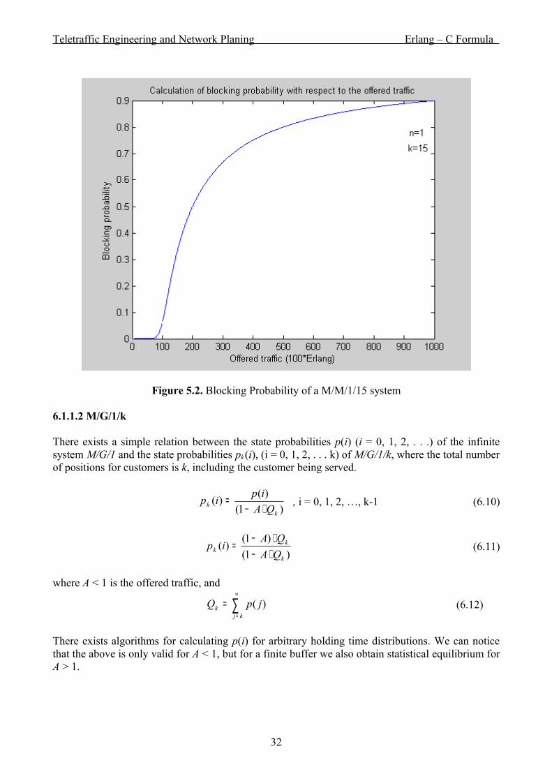
Teletraffic Engineering and Network Planing Erlang – C Formula
Figure 5.2. Blocking Probability of a M/M/1/15 system
6.1.1.2 M/G/1/k
There exists a simple relation between the state probabilities p(i) (i = 0, 1, 2, . . .) of the infinite system M/G/1 and the state probabilities pk (i), (i = 0, 1, 2, . . . k) of M/G/1/k, where the total number of positions for customers is k, including the customer being served.
)1(
)()(k
k QAipip⋅−
= , i = 0, 1, 2, …, k-1 (6.10)
)1()1(
)(k
kk QA
QAip
⋅−⋅−
= (6.11)
where A < 1 is the offered traffic, and
∑∞
=
=kj
k jpQ )( (6.12)
There exists algorithms for calculating p(i) for arbitrary holding time distributions. We can notice that the above is only valid for A < 1, but for a finite buffer we also obtain statistical equilibrium for A > 1.
32

Teletraffic Engineering and Network Planing Erlang – C Formula
6.1.1.3 M/D/1/k
The balance equations for states {0, 1,..,k−2} can be set up in the same way as Fry’s equations of state i.e.
{ } ∑+
=+ +−⋅++=
1
2
),1())(),()1()0()(i
jtttht hjipjphipppip (6.13)
In (6.13), p (j, h) is given by
( ) hj
ejhhjp λλ −⋅=!
),( , j= 0, 1, 2…. (6.14)
It denotes the probability of j news call appearing during the time interval h.
However, it is not possible to write down simple time-independent equations for state k−1 and k. However, the first (k − 2) equations together with the normalization requirement (6.5) and the fact that the offered traffic equals the carried traffic plus the rejected traffic (PASTA property):
)()0(1 kAppA +−= (6.15)
The result is (k+1) independent equations, which could be solved easily.
6.2 Multiple-server system
The state probabilities of the multiple-server finite-buffer system (particularly M/M/n/k) can be obtained in the similar manner as the state probabilities of the infinite buffer system. In a system with n server and k queuing positions we have (k + 1) states (0, 1,…, k).
Typically, in k there are included n queuing positions – those determined by the number of servers. (Alternatively, in some other notation where this is not the case, the number of states are determined by n + k + 1) The state diagram is shown below.
Figure 6.2 State transition diagram for Multiple-server Finite-buffer System
6.2.1 Steady State Probabilities
We can derive the state probabilities of M/M/n/k queuing system in the similar manner as in M/M/n. The relation (2.7) still holds in this case. However, the normalization condition is finite.
33

Teletraffic Engineering and Network Planing Erlang – C Formula
1)(0
=∑=
k
iip (6.16)
1...1!
...!21
1)0( 2
22
=
++++++++ −
−
nk
nkn
nA
nA
nA
nAAAp (6.17)
nA
nA
nA
nA
iA
p
n
i
nkni
≤
−
−
+
=
∑−
=
+−,
1
1
!!
1)0(
1
0
1
(6.18)
Now the state probabilities are as follows:
(6.19)
6.2.2 Blocking Probability – M/M/n/k
The blocking occurs when all servers, together with all waiting positions in the buffer are busy. Therefore, the probability of blocking is equal to p(k).Using (2.7), (6.18), and (6.19), the probability of blocking becomes:
∑−
=
+−
−
−
−
−
+
=
1
0
1
1
1
!!
!)(
n
i
nkni
nk
nkn
nA
nA
nA
iA
nA
nA
blockingp (6.20)
6.2.2.1 MATLAB Code for the Blocking Probability in M/M/n/k
% The following script computes the blocking probability that a system with n servers, k-n % available waiting positions in the buffer, Poisson arrival rate lambda, service rate % mu, and intensity rho = lambda/mu will have with respect to the offered traffic. The % offered traffic is measured in Erlang. It uses the expression (6.20).n =10;k =15;for ro = 1:3000 rho = ro/100; nom (ro) = (rho^n / factorial (n) )*( (rho^(k-n)) / (n^(k-n) ) );
34
≤≤⋅
⋅=
⋅
≤≤⋅=
−
−
kinnnAp
nAnp
niiAp
ip
ni
ini
i
,!
)0()(
0,!
)0()(

Teletraffic Engineering and Network Planing Erlang – C Formula
for i=1:n-1 t (i)=(rho^i) / (factorial(i) ); end s (ro)=sum (t); m (ro)=rho^n / factorial (n); l (ro)=m (ro)*(1-( (rho / n)^(k – n + 1) ) ) / (1- (rho / n) ); denom (ro)=s (ro) + l (ro); pb (ro) = nom (ro) / denom (ro);endplot (pb);xlabel ('Offered traffic (100*Erlang)')ylabel ('Blocking probability')title ('Calculation of blocking probability with respect to the offered traffic')
Figure 6.3. Blocking Probability of M/M/10/15 system
35

Teletraffic Engineering and Network Planing Erlang – C Formula
6.2.3 Queue Length Distribution – M/M/n/k QLD is easy to obtain from (3.6). It is:
)()()...1()2()()1()( KKpLnpLnpLpS δδδ +++++= (6.21)
Similarly,
)()(...)1()()()()(12
NKLnpnALnp
nALnp
nALp
nK
S −+⋅⋅
+++⋅⋅
+⋅⋅=
+−
δδδ (6.22)
−+
+++
+=
−
)(...)1()()()( NKLnAL
nALnp
nALp
nK
S δδδ (6.23)
In terms of Erlang – C, (3.8) can be rewritten as:
−+
+++
+−=
−
)(...)1()()()( ,2 NKLnAL
nAL
nAnAE
nALp
nK
nS δδδ (6.24)
As for the QLD function, following (2.10), we can write:
)(1
1)()(
1
1
npnA
nA
nA
iplLPl
lnk
k
lni
+
−−
++=
−
−
==> ∑ (6.25)
1
,21
1)()()(+−−
++=
−==> ∑
llnk
n
k
lni nA
nAAEiplLP (6.26)
Accordingly,
1
,2 1)(1)(1)(+−−
−−=>−=
llnk
nS nA
nAAElLPLF (6.27)
6.2.3.1. MATLAB Code for PDF and QLD – M/M/n/k
% The following script computes the queue length distribution (QLD) and the respective % probability density function (PDF) that a M/M/n/k system, Poisson arrival rate lambda, % service rate (per server) mu, and intensity A = lambda / mu will have. It should be satisfied % that A > 0, n > 0, A < n, n - positive integer. It uses the expressions (6.24) for PDF% and (6.27) for QTD. Mean service time, measured in time units, offered traffic,
36

Teletraffic Engineering and Network Planing Erlang – C Formula
% measured in Erlang s = 10;mu = 1/s; n = 20;A = 19;k = 35;C=erlangc (n, A);for L=1:k-n ps (L)=( C*(n - A) / n)*( (A / n)^L); Fs (L)=1 - C*( (A / n)^(L + 1) )*(1- (A / n)^(k – n - L) );end stem (ps,'g','o');hold on stem (Fs,'r','x');xlabel ('Queue Length')ylabel ('PDF (green), QLD (red)')title ('Calculation of Probability Density Function and Queue Length Distribution')
Figure 6.4. Queue Length Distribution and its Probability Density Function of M/M/n/k
37

Teletraffic Engineering and Network Planing Erlang – C Formula
6.2.3.2 Mean Queue Length – M/M/n/k Again, the derivation of MQL resembles much to the one in M/M/n case. Consequently, we start out from:
∑ ∑=
−
+=
−+⋅=n
i
nK
nin ipniipL
0 1
)()()(0 (6.28)
ninK
nin n
AnpniL−−
+=∑
−=
1
)()( (6.29)
Moreover,
inK
in n
AinpL ∑−
=
=
2
1
)( (6.30)
Further on,
inK
in n
AnAn
AnpL
∂∂= ∑
−
=
2
1 )/()( (6.31)
We can put the differential operator outside integral. This yields:
inK
in n
AnAn
AnpL
∂∂= ∑
−
=
2
1)/()(
(6.32)
nA
nA
nAnAnpL
nK
n
−
−
∂∂=
+−
1
1
)/()(
12
Finally, solving the derivative, we arrive at
−
+−
−−
−
=
−+−
nA
nAnK
nA
nA
nAnpL
nKnK
n
1
)12(
)1(
1)(
2
2
12
(6.34)
In terms of Erlang – C, (6.41) can expressed by
38
(6.33)

Teletraffic Engineering and Network Planing Erlang – C Formula
+−−
−
−
−=
−
+−
nK
nK
n nAnK
nA
nA
nA
AnnnpL
2
12
)12(1
1)( (6.35)
+−−
−
−
=+−
+−
12
12
,2 )12(1
)(nK
nK
nn nAnK
AnnA
AAEL (6.36)
6.2.4. Waiting Time Distribution – M/M/n/k
The derivation of WTD function follows the line of thought as in the case of M/M/n. The relation (4.3) is also valid here. Since the issue here is WTD function of a finite-buffer system with K+1 steady states, the conditional probability that a customer upon arriving to the system observes all n servers busy and m waiting customers (m = 0,1,2…K-n) now becomes:
∑∑−
=
−
=
=+
+=nK
s
s
m
nK
s
w
nAnp
nAnp
snp
mnpmp
00)(
)(
)(
)()(λ
λ (6.37)
−
−
= +−
nA
nA
np
nAnp
mp nK
m
w
1
1)(
)()( 1
(6.38)
1
1
1)( +−
−
−
= nK
m
w
nA
nA
nAmp
, m = 0,1,2…K-n (6.39)
Now that we have found the conditional probability, we go further onto determining the unconditional waiting time distribution. Therefore,
39

Teletraffic Engineering and Network Planing Erlang – C Formula
∑−
=
=nK
mw mtFmptF
0
)/()()( (6.40)
Furthermore, substituting (4.3) and (6.23) into (6.24), we have
( )∑ ∑−
=
−∞
+=+−
−
−
=
nK
m
tn
ki
i
nK
m
eitn
nA
nA
nAtF
0 11 !
1
1)( µµ
(6.41)
It is very difficult to obtain the solution for this function. However, by utilizing Mathematica 4.2, we arrive at the following expression:
e-nmtI1- AnMIAnM-nIAIAnMK -IAnMnnMJãnmt - ãnmt Gamma@1+k,nmtDGamma@1+kDNI1 -IAnM1+K-nMHA - nL
In (6.42), we have introduced Gamma function. We consider Gamma function in Appendix A.
The PDF function has even more complicated form and therefore, it will not be considered here.
6.2.4.1. Mean Waiting Time – M/M/n/k
Similarly, as in the case of M/M/n, we can apply the Little’s formula to determine MWT. Hence,
(6.43)
Following from (6.27), in terms of Erlang – C, this can be expressed by:
+−−
−
−
==+−
+−
12
12
,2 )12(1
)(1 nK
nK
nn
n nAnK
AnnA
AAEL
Wλλ
(6.44)
40
(6.42)
−
+−
−
−
−
==
−+−
nA
nAnK
nA
nA
LW
nKnK
nn
1
)12(
1
11
2
2
12
λλ
(3.35)
=)(tF

Teletraffic Engineering and Network Planing Erlang – C Formula
7. Cost Function
Moe first derived his principle for queuing systems. He studied the subscribers waiting times for an operator at the manual exchanges in Copenhagen Telephone Company. Let us consider k independent queuing systems. A customer being served at all k systems has the total average waiting time PiWi, where Wi is the mean waiting time of i’th system which has ni servers and is offered the traffic Ai. The cost of a channel is ci, eventually plus a constant cost, which is included in the constant C0 below. Thus the total costs for channels becomes:
∑=
⋅+=k
iii cnCC
10 (7.1)
If the waiting time is also considered as a cost, then the total costs that is to be minimised becomes f = f (n1, n2, . . ., nk). This is to be minimised as a function of number of channels ni in the individual systems. If the total average waiting time is W, then the allocation of channels to the individual systems is determined by:
{ }
−⋅+⋅+= ∑∑
ii
iiik WWcnCnnnf ϑ021 min),...,,(min (7.2)
whereϑ (theta) is the Lagrange’s multiplier.
As ni is integral, a necessary condition for minimum, which in this case also can be shown to be sufficient condition, becomes:
0 < f(n1, n2, . . . , ni-1, . . . , nk) - f(n1, n2, . . . , ni, . . . , nk) , (7.3)
0 ≤ f(n1, n2, . . . , ni, . . . , nk) - f(n1, n2, . . . , n i+1, . . . , nk) , (7.4)which corresponds to:
ϑi
inincAWAW
ii>−− )()(1 (7.5)
ϑi
inincAWAW
ii≤− + )()( 1 (7.6)
where Wni (Ai) is given by (4.15). Expressed by the improvement function for the waiting time FW,n (A) in (5.4) the optimal solution becomes:
),()( ,1, AFc
AFii nW
inW ≥>− ϑ
i =1,2…k (7.7)
The function FW,n (A) is tabulated in Moe’s Principle (Jensen, 1950 [5]). Similar optimizations can be carried out for other improvement functions.
41

Teletraffic Engineering and Network Planing Erlang – C Formula
8. Priority of customers
In real life customers are often divided into N priority classes, where a customer belonging to class p has higher priority than a customer belonging to class p+1. We distinguish between two types of priority:
• Non-pre-emptive (HOL) - A new arriving customer with higher priority than a customer being served waits until a server becomes idle (and all customers with higher priority have been served). This discipline is also called HOL (Head-Of-the-Line).
• Pre-emptive - A customer being served having lower priority than a new arriving customer is interrupted. We distinguish between:
• Pre-emptive resume (PR) - The service is continued starting from the point where it was interrupted.
• Pre-emptive without re-sampling - The service restarts from the beginning with the same service time
• Pre-emptive with re-sampling - The service starts again with a new service time.
The two latter disciplines are applied in for example manufacturing systems and reliability. There are many different queuing models. However, there are only few general results in the queuing theory. Little’s theorem presented is the most general result, which is valid for an arbitrary queuing system. The theorem is easy to apply and very useful in many cases.
In general only queuing systems with Poisson arrival processes are simple to deal with. Concerning queuing systems in series and queuing networks (e.g. computer networks) it is important to know cases, where the departure process from a queuing system is a Poisson process.
These queuing systems are called symmetric queuing systems, because they are symmetric in time, as the arrival process and the departure process are of the same type. If we make a film of the time development, we cannot decide whether the film is run forward or backward.
Systems that deviate most from the classical models are the systems with a single server. However, these systems are also the simplest to deal with. In waiting time systems we also distinguish between call averages and time averages. The virtual waiting time is the waiting time, a customer experiences if the customer arrives at a random point of time (time average).
The actual waiting time is the waiting time, the real customers experiences (call average). If the arrival process is a Poisson process, then the two averages are identical.
42

Teletraffic Engineering and Network Planing Erlang – C Formula
8.1 Analysis of M/M/n/K Queues with Priorities
We shall further outline an approach that may be used to analyse a M/M/n/K queue (n=1, 2.… and K = n, n+1... ∞) which has job classes of multiple priorities. The priority discipline followed may be either non-pre-emptive or pre-emptive in nature, as we have explained before. However, it should be noted that there might be loss of work in the pre-emptive non-resume priority case. Such loss of work will not happen in the case of the other two priorities. Since we assume that the service times are exponentially distributed, they will satisfy the memory-less property and that, therefore, the results will be the same both for the pre-emptive resume and pre-emptive non-resume cases.
For a P priority system, we consider jobs of class 1 to be the lowest priority and jobs of class P to be the highest priority. The job arrivals for class i come from a Poisson process at rate λi. When a job of this class gets served by any of the servers in the queue, the service time is an exponentially distributed random variable with mean μ -1. The traffic of priority class i offered to the queue is denoted by ρ = λ/μ. We consider here queues with both pre-emptive and non-pre-emptive priority disciplines. The approach suggested may be applied to both single-server and multi-server queues. Moreover, queues with both finite and infinite buffers may be analysed using the suggested approach.
In this section, we do not actually do a complete derivation of the state probabilities of a M/M/n/K queue. Instead, we outline the way in which such a queue may actually be analysed by solving its balance equations. As is usual with any M/M/-/- type queue, the basic approach to its solution is to define the system-states appropriately so that a state transition diagram of the queue may be drawn. Using the exponential (memory-less) distribution of the inter-arrival and service times, the probability flows in the state transition diagram are identified. The balance equations are then obtained by choosing proper closed boundaries. Thereafter we equate the flow across each boundary. These balance equations are then solved along with the normalisation condition (i.e. sum of the probabilities of all states equal to unity) to obtain the state probabilities. Once these have been obtained, the performance parameters of interest may be suitably calculated. In the following, we consider the cases of pre-emptive and non-pre-emptive priorities separately. For each case, we first give the analytical approach for the M/M/1 case and then show how it may be used to handle the M/M/1/K queue and the M/M/n/K queue.
8.1.1 M/M/-/- Queue with Pre-emptive Priority
We first consider the simple M/M/1 queue with infinite buffers. This queue may be analysed by drawing a state transition diagram with the states given by the P-tuple (n1,........,nP) where ni is the number in the system of priority class i. Note that the server will always be engaged by a job of the highest priority class present in the system, i.e. by a job of class j with service rate μj if n j ≥ 1 and nj+1 = ..... = nP = 0.
The state transition diagram for a 2-priority M/M/1 queue with infinite buffers operating with a pre-emptive priority discipline is shown in Fig. 7.1. Since all the flows are known, writing and solving the corresponding balance equations with the normalisation condition may find the equilibrium probabilities of each of the states. Some of the balance equations for this case are given below as an example.
43

Teletraffic Engineering and Network Planing Erlang – C Formula
Figure 8.1. State transition diagram for 2-priority M/M/1 queue with pre-emptive priority
Since the rules for transition between the states may be stated logically, we can actually use a computer program to generate the actual balance equations. These equations may then be given to an appropriate mathematical package to get the state probabilities. For the infinite buffer case, we may have some computational difficulties because of the infinite number of states. If this happens to be the case, then a convenient approximation would be to limit the state space to some large values of the total number in the queue and solve this approximate model instead.
This would also actually be the way one can solve a M/M/-/- pre-emptive priority system with finite buffers. As an example, consider the 2-priority M/M/1/3 queue with pre-emptive priority. In this case, the state transition diagram will be as shown in Fig. 7.2. Note that unlike Fig. 7.1, Fig. 7.2 shows all the states of the system. Moreover, the circled states are the ones where the system is full and any jobs arriving in these states will be lost.
Figure 8.2. State transition diagram for a 2-priority M/M/1/3 Queue with Pre-emptive Priority
44
(8.1)

Teletraffic Engineering and Network Planing Erlang – C Formula
The following balance equations may be written for this M/M/1/3 system.
with the normalisation equation as follows
To solve for the state probabilities in this case, we need any nine of the ten equations of (8.2) and the normalisation condition. Note that in this case, the job loss probability (or the blocking probability) will be p1,2 + p2,1 + p3,0 + p0,3.
If the M/M/-/- pre-emptive multi-priority queue has more than one server, then that can be taken into account while drawing the state transition diagram. Specifically, consider the situation where there are nP jobs of priority class P and c servers in the system. If c < nP then all the servers will be taken by c of the nP (class P) jobs and no free servers will be available for lower priority jobs (if any). In this case, the overall service rate will be c.
On the other hand, if c > nP, then the nP high priority jobs will each get a server and their overall service rate will be nP·μP. The remaining (c-nP) servers will be available for the jobs of priority class P-1 and lower and will be used by these jobs according to the number in these classes. This approach will allow us to define the flows between each of the states in the state transition diagram. Note that the representation of states in the state transition diagram may still be done as the P-tuple (n1,........,nP) where ni is the number in the system of priority class i.
Since the priority discipline is pre-emptive, we do not need to separately specify the priority classes of the jobs engaging the servers. An example of this approach for obtaining the state transition diagram of a M/M/2/3 queue is shown in Fig. 7.3. Using this, one can follow the same solution approach as the one outlined for the M/M/1/3 queue earlier to obtain the various state probabilities.
45
(8.2)
(8.3)

Teletraffic Engineering and Network Planing Erlang – C Formula
Figure 8.3. State transition diagram for a Pre-emptive 2-priorityM/M/2/3 Queue
8.1.1.1 Mean Waiting Time for Pre-emptive Resume Queuing Discipline – M/M/n
We now assume that an ongoing service is interrupted by the arrival of a customer with a higher priority. Later the service continues from where it was interrupted. This situation is typical for computer systems, which will be covered by a concrete example later in this section. For a customer with the priority p there is no customer with lower priority. The mean waiting time Wp for a customer in class p consists of two contributions.
• Waiting time due to customers with higher or same priorities that are already in the queuing system. This is the waiting time experienced by a customer in a system without priority where only the first p classes exists:
'1 p
p
AV− , where ∑
=
⋅=p
ii
ip mV
1,22
λ (8.4)
is the expected remaining service time due to customers with a higher or the same priority and '
pA is given by
∑=
=p
iip AA
0
' (8.5)
• The waiting time due to the customers with higher priority who arrive during the waiting time or service time and overtake the customer considered:
∑−
=−⋅+=⋅⋅+
1
1
'1)()(
p
ipppiipp AsWssW λ (8.6)
We thus get:
'1' )(
1 −⋅++−
= pppp
pp AsW
AV
W (8.7)
46

Teletraffic Engineering and Network Planing Erlang – C Formula
This can be rewritten as follows:
( )'
1''
1 1)1( −− ⋅+
−=− pp
p
ppp As
AV
AW (8.8)
resulting in:
pp
p
pp
pp s
AA
AAV
W '1
'1
''1 1)1()1( −
−
− −+
−⋅−= (8.9)
In the same way we may write the formula for the average waiting time for the SJF–queuing discipline with pre-emptive resume. The total response time becomes:
sWT ppp += (8.10)
8.1.1.2 Mean Queue Length for Pre-emptive Resume Queuing Discipline – M/M/n
The main waiting time in this case can be easily obtained by using the Little’s theorem since it is valid for all queuing systems. It gives the following expression.
−+
−⋅−=⋅=
−
−
−p
p
p
pp
ppp s
AA
AAV
WL '1
'1
''1 1)1()1(
λλ (8.11)
8.1.2 M/M/-/- Queue with Non-Pre-emptive Priority
The basic approach to analysing an M/M/-/- queue with a non-pre-emptive priority discipline would be fairly similar to the approach suggested for the case where the priority discipline is pre-emptive in nature. The state definition would need to be modified in this case in order to describe the job class currently being served for each of the servers.
This is required, as unlike the M/M/-/- queue with pre-emptive priority, the ongoing service (if any) is not interrupted in the non-pre-emptive case because of the arrival of a job of a higher priority class than the one currently being served at a server (when no free servers are available).
For a M/M/n/K queue with P priority classes of jobs, a possible state descriptor would be a (P + n)-tuple of the following form.
State Representation - (n1, ......., nP, s1, ......, sn) where nj is the number of jobs of class j in the system j=0,1,....,P and sk represents priority class of the service currently on-going at server k (k=1,.....,n). Note that n1+......+nP ≤ K for a finite capacity system.
47

Teletraffic Engineering and Network Planing Erlang – C Formula
An alternative representation using a 2P-tuple may give a more compact representation if the number of priority classes is less than the number of servers. In this alternative approach, the state description will be of the following form.State Representation - (n1, ......., nP, s1, ......, sP) where nj is the number of jobs of class j in the system j=0,1,....,P and sk represents the number of servers currently busy serving jobs of priority class k, ( k=1,.....,P).
As an example, we consider using the first method of representation to represent the states of a M/M/1/3 2-priority queue following a non-pre-emptive priority discipline. The state diagram for this queue is shown in Fig. 8.4.
Figure 8.4. State transition diagram for a 2-Priority, Non-pre-emptive M/M/1/3 Queue
For this, we can write balance equations in the same way as it was done earlier. These are given in (8.4).
48
(8.4)

Teletraffic Engineering and Network Planing Erlang – C Formula
We would need any twelve of the thirteen equations of (8.4) along with the normalisation condition
to obtain the actual state probabilities. Once these have been calculated, one can use them to obtain the usual queue performance parameters. Note that, in this case, the loss probability will be given by (p0,3,2+ p3,0,1 + p1,2,2 + p2,1,2 + p1,2,1 + p2,1,1) as the sum of the probability of all those states where the system is full, i.e. the total number in the system is three for this M/M/1/3 queue.
As for the case of the M/M/-/- queue with pre-emptive priority classes, the approach given above for the non-pre-emptive M/M/1/3 queue may also be generalised. Using the same approach, one can also analyze queues where
• The number of priority classes are more than two• The buffer capacity is infinite• The queue has more than one server.
Note that the complexity of the approach suggested here is basically because of the large number of states in the state transition diagram and the resultant complexity in the balance equations. Since the rules for transitions between states are straightforward, one can actually use a computer program to identify the transitions between states and directly write the corresponding balance equations. Using an appropriate numerical package to get the actual state probabilities, even if it is large, may directly solve this set of equations. These may then be used to obtain the queue performance parameters required.
8.1.2.1 Mean Waiting Time for Non-pre-emptive Queuing Discipline (M/M/n)
We may also generalise Erlang classical waiting time system M/M/n with non–pre-emptive queuing disciplines, when all classes of customers have the same exponentially distributed service time distribution with mean value s = µ−1. Denoting the arrival intensity for class i by λi,, we have the mean waiting time Wp for class p:
∑ ∑=
−
=
+⋅+=p
i
p
iipip n
sWLnsVW
1
1
1
λ (8.6)
∑ ∑=
−
=
+⋅⋅
+⋅=p
i
p
iipi
inp n
sWWn
snsAEW
1
1
1,2 )( λ
λ (8.7)
A is the total offered traffic for all classes whereas V is the residual service time for the customer under service when the customer we consider arrives. It is given by the following formula.
∑=
⋅=N
ii
i mV1
22λ
(8.8)
49
(8.5)

Teletraffic Engineering and Network Planing Erlang – C Formula
In (8.8) im2 is the second moment of the service time distribution of the i’th class. The probability E2,n (A) for waiting time is given by Erlang-C formula, and customers are terminated with the mean inter-departure time s/n when all customers are busy. In general we find:
[ ] [ ]''1
,2 )(
pp
np AnAn
AEsnW
−⋅−⋅⋅
=−
(8.9)
8.1.2.2 Mean Queue Length for Non-pre-emptive Queuing Discipline (M/M/n)
Similar with the mean waiting time for pre-emptive resume queuing discipline we can also apply here the Little’s theorem in order to give the expression for the mean waiting for M/M/n with non-preemptive priority.
[ ] [ ]
−⋅−⋅⋅
=⋅=−
''1
,2 )(
pp
npp AnAn
AEsnWL λλ (8.10)
8.2 Concrete example for a Non-pre-emptive Priority System
The explosion of data-intensive applications and high quality of service requirements has caused a change in traditional storage systems. The server-to-disk approach is being replaced by storage area networks (SAN). Emerging as a data communication platform, SAN interconnect servers and storage devices to create a pool of storage that users can access directly. A storage-networking environment consists of three components: servers, storage devices (disks) and interconnect devices. In this section, we propose an analytical model for disks in SAN. Assuming a finite disk buffer and non-pre-emptive priority of read requests over write requests, we model a typical disk in SAN as a 2-priority M/M/1/N queue and evaluate its performance measures such as the blocking probability and response times for both read and write requests. In traditional storage systems, each server has its own private connection to storage, as illustrated in Fig. 8.5. Servers and clients share a communication network, which is used both for messaging and I/O related traffic. However, such a storage system is now suffering from problems such as unavailability of data in case of a failure on server, bandwidth saturation during backups and many other limitations when implementing large configurations.
Figure 8.5 A traditional storage system
50

Teletraffic Engineering and Network Planing Erlang – C Formula
Traditional storage systems are replaced rapidly by storage area networks (SAN). Essentially, SAN uncouple storage devices from the LAN and put them on their own network (Fig. 8.6). A high-speed network similar to LAN, SANs can interconnect technologies similar to the ones used in LANs, namely hubs and switches. SANs provide easy access for multiple servers to multiple storage devices (such as disks, disk arrays, and tape drives) in the same way that LANs allow the client easy access to many servers. SANs enable storage to be externalized from the server and hence allow storage to be shared among multiple servers without impacting the performance of the primary communication network. SANs improve traditional storage systems in many aspects such as computer clustering, topological flexibility, fault tolerance, high availability, and remote management.
Figure 8.6 A typical SAN environment
Disks are a central part of a SAN, which communicate with the server by means of two I/O operations: read and write operations. Modelling disks in a SAN is a difficult task because of the burst I/O arrival patterns and complicated response times for I/O requests. In order simulation modelling of disks in SANs to be simplified it is assumed equal priority of read and write requests, while in reality read requests should have higher priority than write requests in order to improve read response time. Moreover it could be also considered that the disk buffer has infinite capacity, which is unreasonable in practice. Below in this section, we present an analytical queuing model for disks in a SAN by considering a non-pre-emptive priority policy with read requests having higher priority than write requests, and finite disk buffering.
8.2.1 Disks in SAN
Physically a SAN consists of three main components: server systems, storage devices (mainly magnetic disks) and interconnect devices including the interconnect network (switch fabric). Both servers and disks are attached to the interconnect network by means of a network interface card.
8.2.1.1 Read and Write Requests
Servers initiate the communication with disks. Disks take actions according to the requests previously sent by servers. For I/O read requests, the server first sends a request message to the selected disk indicating the number of sectors required, and the initial sector address in the disk. Once the disk has processed the request, it accesses the information, and finally sends the data back to the server through the storage network. The I/O read request lasts since the server initiates it until
51

Teletraffic Engineering and Network Planing Erlang – C Formula
the total amount of data is received at the server. For the I/O write requests, servers start them by sending the data and the initial sector address to the selected disk. Once the data is stored, the disk sends back an acknowledge message to the server. The I/O write request lasts since the server initiates it until the acknowledgement is received.
Both the acknowledgement for write requests and the read request are short messages of a small amount of bytes (typically 16 or 32 bytes). The size of data messages usually ranges from a few bytes, say, 1, 2, 4 or 8 KB, until several KB (32 or 64 KB).
8.2.1.2 Disk Response Time
The disk response time of an I/O request includes three main components: seek time, rotational latency, and transfer time. Seek time is modelled by the function:
cxbxa +−+− )1(1 (8.11)
where x is the distance in cylinders. Coefficients a, b and c depend the disk geometry. Rotational latency lasts since the disk head arrives at the selected cylinder until the first sector of the request passes under the head.
Finally, transfer time is the time needed to transfer the data from/to the disk to/from the disk buffer.
8.3 Analysis Model
In this section, we present a finite queuing model for a typical disk in SAN and evaluate its performance measures such as the blocking probability and mean response time. The state transition diagram for N = 3 is same as that in Fig. 8.3.
8.3.1 Basic Assumptions
We model a typical disk in a SAN by a single server queue with a FIFO discipline. We assume the disk buffer is finite with size for N requests. Disk response depends on the operation type requested by the server. If it is a read request, the disk sends the data back to the server. On the other hand, if it is a write request, only the acknowledgement message is generated.
To improve read response time, we assume read requests have non-pre-emptive priority over write requests. To achieve a tractable model, we make the following simplifying assumptions. Both read and write requests arrive at the disk according to a Poisson process with rate λ1 and λ2, respectively.
We assume the disk response time for both read and write requests to be exponentially distributed with mean 1/µ1 and 1/µ2, respectively.
52

Teletraffic Engineering and Network Planing Erlang – C Formula
8.3.2 Finite Queuing Model
8.3.2.1 State Probabilities
The disk can be modelled as a 2-priority M/M/1/N queue (non-pre-emptive priority). The state representation is a 3-tuple in the form (n1, n2, s). Here, n1 and n2 represent the number of write and read requests, respectively, and s (s = 0, 1, 2) indicates the server is now empty, serving a read request and serving a write request, respectively. There is only one state corresponding to s = 0, which is the initial state (0,0,0) and will be simplified as 0 hereafter. Note that. n1 + n2 ≤ N. Let us take N = 3 for example. The approach can be easily extended in the usual fashion to other bigger values of N. In case N = 3, there are a total of 13 states, whose transition diagram is shown in Fig.8.3. The balance equations for this non-pre-emptive queue and the normalization condition are the same to that from (8.4) and (8.5), respectively.
8.3.2.2 Performance Measures
We are interested in the following performance measures:
• 1N : the mean number of write requests;
• 2N : the mean number of write requests;
• N : the mean number of requests;
• Tp : the mean throughput of the server;
• T : the mean response time of requests;
• PB : the blocking probability.
A little thought will show that
53
(8.12)

Teletraffic Engineering and Network Planing Erlang – C Formula
By Little’s law, the mean response time of requests is
A new request (either write or read) will be blocked when n1 + n 2 = 3. Thus, the blocking probability PB is
8.3.2.3 Numerical Results
In this section, we present numerical results to illustrate our analytical model. In Fig. 8.7 and 8.8, we fix λ2 = 1, µ1 = 15, µ2 = 20 and let λ1 increase from 1 to 10. We see that both blocking probability and mean response time are increasing as λ1 increase. In Figures 8.9 and 8.10, we fix λ1 = 1, µ1 = 15, µ2 = 20 and let λ2 increase from 1 to 10. Again we see that both blocking probability and mean response time are increasing as λ2 increases.
Figure 8.7 Blocking Probability (Fixed λ2) Figure 8.8. Mean Delay (Fixed λ2)
Figure 8.9 Blocking Probability (Fixed λ1) Figure 8.10. Mean Delay (Fixed λ1)
54
(8.13)
(8.14)

Teletraffic Engineering and Network Planing Erlang – C Formula
9. Systems with Limited Waiting Tme
We often need strategy for limiting the number of customers in the system. One solution is to impose an upper limit to the allowed waiting time. This may be due to impatient customers, which give up waiting, or due to that the system enforces them to leave the queue.
In the following we consider Erlang delay system M/M/n having Poisson arrival process (λ), exponential service times (μ), n servers and FCFS-queuing discipline.
9.1 Exponentially distributed Time-out Interval
Typical example of a queuing system with limited waiting time is Palm's waiting time model, where customers in queue leave the system with rate μr. We then get a system with arrival rates λi, respectively departure rates μr, in state i:
λλ =i , ∞<≤ i0 (9.1)
⋅−+⋅⋅
=,)(
,
ri nin
iµµ
µµ
This system is a classical queuing system, where waiting customers becomes impatient and leave the system after an exponentially distributed waiting time. The classical systems are special cases of this:
0=rµ : Erlang's waiting time system , µµ =r : Molina's Lost-Calls-Held system , ∞=rµ : Erlang's Lost-Calls-Cleared system .
9.2 Constant Time-out Interval
A time-out interval is often applied in technical systems after a constant time interval. In old switching systems this was implemented by heating a resistor, in new digital switching systems it is implemented by software.
For example, the dial tome is terminated, if no dialling takes place within approximately 10 seconds. Also, it is only possible to give ringing tone to a B-subscriber during a limited time interval (2-3 minutes) if there is no answer.
55
inni
≤≤≤ ,0 (9.2)

Teletraffic Engineering and Network Planing Erlang – C Formula
9.2.1 State Probabilities – Systems with Constant Time-out Interval
It has been shown that the state probabilities satisfy the following relations:
!)0()(
iApip
i
⋅= p(i) , 0 ≤ i ≤ n (9.3)
∏= +
+⋅
⋅=+i
j jn
i
cn
npinp
1
1)()(
µ
λ
, 1 ≤ i ≤ ∞ (9.4)
In terms of Erlang – C:
∞≤≤
+
−=+
∏= +
i
cn
nAnAEinp
i
j jn
in 1,
1)()(
1
,2
µ
λ
(9.5)
From (8.4) we can see that the state probabilities become increasingly complicated as i approaches infinity. Even for small values of i, the expressions are much difficult. To elaborate, we present the first value for i = 1.
)2
(
)4
exp(
)()1(2,2
τµ
µ τ
πµµ
λ
Erfn
nAnAEnp n
−+
−=+
(9.6)
9.2.2 Queue Length Distribution – Systems with Constant Time-out Interval
The probability density function of the QLD is determined by the same expression as in the M/M/n case.
...)1()2()()1()( +++++= LnpLnpLpS δδ (9.7)
However, since the state probabilities are so complicated it will not be presented in further detail. The same goes for QLD. Only the general idea is given below.
∑∞
++=
−=>−=1
)(1)(1)(lni
S iplLPLF (9.8)
56

Teletraffic Engineering and Network Planing Erlang – C Formula
9.2.2.1 Mean Queue Length - Systems with Constant Time-out Interval
Utilizing the well-known relation for determining QLD i.e.
∑ ∑=
∞
+=
−+⋅=n
i nin ipniipL
0 1
)()()(0 (9.9)
∑∞
+=
−=1
)()(ni
n ipniL (9.10)
This is also very complicated to derive, so we will not go any further.
9.2.3. Waiting Time Distribution - Systems with Constant Time-out Interval
We consider Erlang delay system (n, λ, μ) and choose the mean service time 1/ μ as time unit. We introduce the additional assumption that waiting calls give up waiting after a constant time interval τ, and that the queuing discipline is FCFS. It can be shown that the waiting time distribution for this becomes:
τ⋅−−
−−
⋅⋅−
⋅−=
)(,2
)(,2
)(1
)(1)(
Ann
tAnn
eAEnA
eAEtW (9.11)
The formula (9.11) is valid only for A ≠ n. When A > n the exponent becomes positive, and E2 (A ) = E 2,n (A) should not be considered as a probability, but simply as a values obtained from (2.22).
[ ])(1)(
)(,1
,1,2 AEAn
AnEAE
n
nn −⋅−
= (9.12)
where E1=E1,n (A) is Erlang-B formula, which is valid for all A > 0. By inserting this in (9.11) we get
[ ][ ] τ)(
11
)(11
)()(1)()(1
)( An
tAn
eAEAAEAneAEnAEAntW −−
−−
⋅⋅−−−⋅⋅−−−
= (8.13)
For t = τ = 0, W (0) becomes equal to the probability for experiencing a waiting time zero, i.e. immediate service, which in this case as expected becomes 1 – E1,n (A).
For τ → ∞, we must demand that A < n, and we find the waiting time distribution for the Erlang-C system (4.11). In the general case 0 < T < ∞ we get from (9.11):
57

Teletraffic Engineering and Network Planing Erlang – C Formula
τ)(2
2
)(1
)(1)0()(
AneAEnA
AEWimmediatep−−⋅⋅−
−==
(9.14)
{ } { }ττ <Τ−==Τ= p1p e)p(immediat
τ
τ
τ)(
2
)(2
)(1
)(11)(1)(
An
An
eAEnA
eAEWimmediatep−−
−−
⋅−
⋅−−=−= , A ≠ n (9.15)
For A = n we cannot calculate E2 = E2,n(A), because A - n appears in the denominator. If we apply the expression (9.13), both the numerator and the denominator becomes equal to zero for A = n. Therefore, we apply I'Hospital rule and differentiate numerator and denominator separately with respect to A. The derivative of Erlang-B formula for A = n becomes:
21
211
1'1 1 EEE
An
AEE =+⋅
−=
∂∂
= for A = n (9.16)
We thus get:
)()()(
AgAftW = (9.17)
[ ] τττ )('1
)(1
'11
)('1
)(1
'11
1)1()1(
)()(
AnAn
tAntAn
eAEeAEEAEenEetEnEAE
AgAf
−−−−
−−−−
⋅⋅−⋅⋅+−⋅+−−⋅⋅−⋅⋅⋅−⋅+−−
= (9.18)
As A approaches n, both f (A) and g' (A) has a limit value different from zero, and according to I' Hospital's rule W(t) will have the limiting value:
)()(lim)(lim '
'
AgAftW
nAnA →→= (9.19)
11)1(
)(lim1
1
+⋅⋅+−⋅
=→ τEA
tAEtWnA
, A = n, 0 ≤ t ≤ τ (9.20)
Following the line of thought as in the previous sections, we can derive the probability density function (PDF) as the derivative from waiting time distribution (WTD). Hence,
τ)(,2
)(,2
)(1
)()()(
Ann
tAnn
S
eAEnA
eAEAntp
−−
−−
−
−= (9.21)
58

Teletraffic Engineering and Network Planing Erlang – C Formula
9.2.3.1 MATLAB Code for PDF and WTD of Systems with Constant Time-out Interval
% The following script computes the waiting time distribution (WTD) and the respective % probability density function (PDF) that a system with n servers, constant time-out interval,% finite waiting line, Poisson arrival rate lambda, service rate (per server) mu, and intensity % A = lambda / mu will have. It uses the expressions (9.21) for PDF of WTD and (9.11) for % WTD. Mean service time s, measured in time units, time-out interval in time units s=1; mu = 1/s; n = 20; tau = 3;A = 19; L = 15;C = erlangc (n, A);t = 0:0.25:L;nom_ps = (n - A)*C*exp (- (n - A)*t);nom_Fs = 1-C*exp (- (n - A)*t);denom = 1 - (A / n)*C*exp (- (n - A)*tau);ps = nom_ps / denom; Fs = nom_Fs / denom;ps (4*tau: 4*L) = 0;Fs (4*tau: 4*L) = 1;plot (t, ps, 'g');hold onplot (t, Fs, 'r');xlabel ('Waiting time (Time Units)')ylabel ('PDF (green), WTD (red)')title ('Calculation of Probability Density Function and Waiting Time Distribution')
Figure 9.1. Waiting Time Distribution and its Probability Density Function of an M/M/n
59

Teletraffic Engineering and Network Planing Erlang – C Formula
System with Constant Time-out9.2.3.2. Mean Waiting Time - Systems with Constant Time-out Interval
MWT will not be calculated in detail since it is extremely difficult to do that. We should only confirm the Little theorem.
∑∞
+=
−==1
)()(1ni
nn ipni
LW
λλ (9.22)
60

Teletraffic Engineering and Network Planing Erlang – C Formula
10. Concluding Remarks
Upon reading this report one can notice that the emphasis is placed on derivation of Erlang - C and some different representations of the formula as well. Furthermore, we concentrate on different queue configurations, such as: M/M/n and M/M/n/k. We investigated the waiting time and queue length distribution for both of them as well as their expression for the mean values. It also involves having a good understanding of queuing and probability theory.
However, there are several occasions when it is often hard or impossible to analyze some of the queuing systems in an exact analytical way. For instance, in the case of M/M/n with constant time-out interval, the final formulae for queue length distributions as well as the mean waiting time and mean queue length were not derived. Also, this applies to systems with finite number of waiting positions. This is something we have encountered during our work on this mini-task.
61

Teletraffic Engineering and Network Planing Erlang – C Formula
Appendix A – Gamma Function
The (complete) gamma function Γ(n) is defined to be an extension of the factorial to complex and real number arguments. It is related to the factorial by Γ (n) = (n-1)!. It is analytic everywhere except at z = 0, -1, -2, ... and the residue at z = - k is
!)1()(Re
kzs
k
kz
−=Γ−=
(1)
There are no points z at which Γ(z) = 0. The graphical representation of the gamma function is given on Fig. 1.
Figure 1. Gamma Function
The gamma function can be defined as a definite integral for [z] > 0 (Euler's integral form).
∫ ∫∞
−∞
−−− ==Γ0
12
0
1 2
2)( dttedtetz zttz (2)
or 11
0
1ln)(−
∫
=Γ
z
tz (3)
62

Teletraffic Engineering and Network Planing Erlang – C Formula
Appendix B - Error Function
Erf(z) is the "error function" encountered in integrating the normal distribution (which is a normalized form of the Gaussian function). It is defined by
∫ −=z
t dtezerf0
22)(π
(4)
The graphical presentation of the error function is given on Figure 2.
Figure 2. Error Function
63

Teletraffic Engineering and Network Planing Erlang – C Formula
Glossary of Acronyms
ATM Asynchronous Transfer ModeFCFS First Come First ServedFIFO First In First OutHOL Head Of LineIP Internet ProtocolLAN Local Area NetworkLCFS Last In First Served LIFO Last In First OutMQL Mean Queue Length MWT Mean Waiting TimePASTA Poisson Arrivals See Time AveragePCT-I Pure Chance Traffic Type OnePDF Probability Density FunctionQLD Queue Length DistributionSAN Storage Area NetworksSIRO Service In Random OrderWTD Waiting Time Distribution
64
Teletraffic Engineering and Network Planing Erlang – C Formula
References:
[1] Villy B. Iversen (2004): Teletraffic Engineering and Network Planning
[2] Huebner, F. (1998), Global Telecommunications Conference, (GLOBECOM 98), The Bridge to Global Integration.IEEE , Volume: 1 (8-12 Nov. 1998) : On the accuracy of approximating loss probabilities in finite queues by probabilities to exceed queue levels in infinite queues
[3] Raif O. Onvural (1990): Survey of Closed Queuing Networks with Blocking
[4] Arne Jensen (1950): Moe’s Principle
[5] Guoping Zeng, Imrich Chlamtac and Hua Zhu (Center for Advanced Telecommunications Systems and Services The University of Texas at Dallas): Performance Modeling of Disks in Storage Area Networks
[6] Wei-Bo Gong; Glasserman, P. (1988), Proceedings of the 27th IEEE Conference on 7-9 Dec. 1988: Infinitesimal perturbation analysis of the M/G/1/K queue
[7] K.R. Krishnan (1990), IEEE Transactions on Communications, Vol. 38, No 9 September 1990: The Convexity of Loss Rate in an Erlang Loss System and Sojurn in an Erlang Delay System with respect to Arrival and Service Rates
[8] Duan-Shin Lee, C&C Research Laboratories, NEC USA Inc.: A Generalized Non-pre-emptive Priority Queue
[9] Error function - Mathworld website: http://mathworld.wolfram.com/Erf.html
[10] Gamma function - Mathworld website: http://mathworld.wolfram.com/GammaFunction.html
65