erlang-r: a time-varying queue with reentrant...

MANUFACTURING & SERVICEOPERATIONS MANAGEMENT

Articles in Advance, pp. 1–17ISSN 1523-4614 (print) � ISSN 1526-5498 (online) http://dx.doi.org/10.1287/msom.2013.0474

© 2014 INFORMS

Erlang-R: A Time-Varying Queue with ReentrantCustomers, in Support of Healthcare Staffing

Galit B. Yom-Tov, Avishai MandelbaumTechnion–Israel Institute of Technology, Technion City, Haifa 32000, Israel

{[email protected], [email protected]}

We analyze a queueing model that we call Erlang-R, where the “R” stands for reentrant customers. Erlang-Raccommodates customers who return to service several times during their sojourn within the system, and

its modeling power is most pronounced in time-varying environments. Indeed, it was motivated by health-care systems, in which offered-loads vary over time and patients often go through a repetitive service process.Erlang-R helps answer questions such as how many servers (physicians/nurses) are required to achieve prede-termined service levels. Formally, it is merely a two-station open queueing network, which, in a steady state,evolves like an Erlang-C (M/M/s) model. In time-varying environments, on the other hand, the situation dif-fers: here one must account for the reentrant nature of service to avoid excessive staffing costs or undesirableservice levels. We validate Erlang-R against an emergency ward (EW) operating under normal conditions aswell as during a mass casualty event (MCE). In both scenarios, we apply time-varying fluid and diffusionapproximations: the EW is critically loaded and the MCE is overloaded. In particular, for the EW we propose atime-varying square-root staffing policy, based on the modified offered-load, which is proved to perform wellover small-to-large systems.

Keywords : healthcare; queueing networks; modified offered-load; time-varying queues; Halfin–Whitt regime;QED regime; ED regime; emergency department staffing; mass casualty events; patient flow

History : Received: August 18, 2011; accepted: November 8, 2013. Published online in Articles in Advance.

1. Introduction: The Erlang-R ModelIt is natural and customary to use queueing mod-els in support of workforce management. Most com-mon are the Erlang-C (M/M/s), Erlang-B (M/M/s/s),and Erlang-A (M/M/s+M) models, all used, for exam-ple, as models of call centers. But when consid-ering healthcare environments, we find that thesemodels lack a central prevalent feature, namely, thatcustomers might return to service several times dur-ing their sojourn within the system. Therefore, the ser-vice offered has a discontinuous nature, because it isnot provided at a single event. This has motivated ourqueueing model, (the time-varying) Erlang-R (“R” forreentrant customers or repetitive service), whichaccommodates the return-to-service phenomena.

More explicitly, we consider a model where cus-tomers seek service from servers. After service is com-pleted, with probability 1 − p they exit the systemand with probability p they return for further service,after a random delay time. We refer to the servicephase as a needy state and to the delay phase as a con-tent state (following Jennings and de Véricourt 2011).Thus, during their stay in the system, customers startin a needy state and then alternate between needyand content states. We assume that there are multi-ple servers in the system, and their number st canvary with time. When customers become needy and

a server is idle, they are immediately treated by aserver. Otherwise, customers wait in queue for anavailable server. The queueing policy is FCFS (first-come first-served). Needy service times are indepen-dent and identically distributed (i.i.d.), with generaldistributed G1 and mean 1/�, and content times arei.i.d. with general distribution G2 and mean 1/�. Wealso assume that the needy and content times areindependent of each other and of the arrival process.The arrival process is a time-inhomogeneous Poissonprocess with rate function �t , t ≥ 0; this is empiricallyjustified, for example, in Maman (2009). Some of ourresults require that the needy and content times haveconcrete distributions (exponential, deterministic). Weshall state specifically when this is the case. Figure 1displays our system schematically.

1.1. Examples of Service Systems withReentrant Customers

We now describe examples that underscore the prac-tical relevance of Erlang-R: An emergency ward (EW)under normal conditions or during a mass casualtyevent (MCE), the radiology reviewing process, oncol-ogy bed management, and call centers.

The first example captures the complex medi-cal service process, provided by EW physicians (ornurses) (Marmor and Sinreich 2005). We consider

1

Yom-Tov and Mandelbaum: The Erlang-R Queue2 Manufacturing & Service Operations Management, Articles in Advance, pp. 1–17, © 2014 INFORMS

Figure 1 The Erlang-R Queueing Model

Needy(st-servers)

rate �

Content(delay)rate �

1–p

p

1

2

ArrivalsPoisson (�t)

Patient discharge

separately normal and stressful EW conditions. Forthe first, the process starts by admitting patientsand referring them to an EW physician. The physi-cian examines them to decide between dischargeversus hospitalization—a decision that could requirea series of medical tests. Thus, the process that apatient experiences, from the physician’s perspective,fits Erlang-R: a physician visit is a needy state; andbetween each visit, the patient is in a content state,which represents the delay caused by undergoingmedical tests such as X-rays, blood tests, or exami-nations by specialists. After each visit to the physi-cian, a decision is made to release the patient from theEW (home or hospitalized), or to direct the patient toadditional tests. We shall verify later, in §6, that thesimple Erlang-R model captures the essence of the com-plete EW process, enough to render the model usefulfor staffing applications.

EWs often accommodate MCEs, and these areinherently transient (Cohen et al. 2013). Based ondata from an MCE drill, as described in §7.1, wedemonstrate that our time-varying Erlang-R can accu-rately forecast MCE census and hence support itsmanagement. Ours is a chemical MCE, and theseshare treatment protocols that are especially amenableto Erlang-R modeling: every T minutes or so, eachpatient must be monitored and given an injection,where T depends on severity. (In our case, patientswere triaged into four levels of severity: the mostacute required treatment every 10 minutes, the secondlevel every 30 minutes, etc.)

Our second example is the radiology reviewingprocess (Lahiri and Seidmann 2009). After a mam-mography test, the radiologist interprets the results.In some cases, part of the information on the patientis lacking: the radiologist starts the reviewing butthe case must be put on hold. One then waits forthis additional information to arrive, after whichthe reviewing process starts again. With radiologistsbeing the servers, this can be modeled using ourneedy–content cycle.

The third example is the process of bed manage-ment in an oncology ward. In such a medical ward,patients return for hospitalization and treatment farmore frequently than in regular wards. Here servers

are the beds, the needy state models the times whena patient is in the hospital, and the content state cor-responds to a patient being at home. A patient leavesthe system when cured or unfortunately passes away.(A hospital colleague tells us that the same dynam-ics could possibly fit a geriatric ward during theflu season, when elderly patients transfer back andforth between their (nursing) home and the hospital.)Lessons from fitting Erlang-R to this and the aboveexamples are summarized in §8.

Our prime motivation is healthcare, yet, Erlang-Ris clearly relevant to other environments, for exam-ple, call center customers who return for additionalservices (Zhan and Ward 2012, Khudyakov et al.2010). Note that our reentrant customers differ fromwhat is traditionally referred to as retrial customersin queueing theory (redials in call centers) (e.g., Falinand Templeton 1997): these leave the system priorto service, in response to all lines being busy orafter abandonment because of impatience, whereasour customers return after service and their returnsare considered part of the service process.

1.2. ContributionsThe contributions of our paper are both theoreticaland practical. The main ones are as follows:

Theoretical understanding of the significance of reen-trance, leading to practical insights for the above healthcareexamples (§8). A central question is when must cus-tomer returns be acknowledged explicitly, as opposedto being absorbed within the service or arrival process.(This absorption has been common practice; see, e.g.,Green et al. 2006.) Our important insight (§§3 and 4)is that returns become significant in time-varying sys-tems (they are not so in a steady state)—roughlyspeaking, when the arrival rate varies noticeably dur-ing the sojourn-time of a customer within the sys-tem (§4.2). In particular, with periodic arrivals andexponential services, this significance is most pro-nounced when the period duration of the arrivalprocess is around

√

��41 − p5 (§4.3); another insightis that reentering customers smooth (reduce theamplitude of) staffing requirements over time (Theo-rem 5); the lessons are similar for deterministic servicetimes but the story is then somewhat more complex(see §EC.1.5 of the Internet supplement, available athttp://dx.doi.org/10.1287/msom.2013.0474).

Stabilizing performance of time-varying queueing net-works via square-root staffing (SRS) rules (§5). Signifi-cantly, this has been so far proved feasible only forisolated queues (Jennings et al. 1996, Feldman et al.2008, Whitt 2013). As explained below, the networkfor which performance is stabilized could be rathergeneral—for example, the full-fledged EW networkin §6. Our method requires explicit calculations of thetime-varying offered-load, based on Massey and Whitt

Yom-Tov and Mandelbaum: The Erlang-R QueueManufacturing & Service Operations Management, Articles in Advance, pp. 1–17, © 2014 INFORMS 3

(1993), as well as of key performance measures forErlang-R (§§3 and 4).

Analytical approximations for the queue-length andnumber-of-busy-servers processes. These are derived sep-arately for systems that are supercritical (e.g., EWsduring MCEs as described in §7) by implementingmethods from Mandelbaum et al. (1998), or systemsthat are well balanced, namely, quality and efficiencydriven (QED; see the Internet supplement, §EC.3,which is a manifestation of the modified-offered-load(MOL) principle as in Massey and Whitt 1994).

Developing and implementing a complete framework forassessing the practical value of asymptotic queueing the-ory. This framework entails four network models:queueing, fluid, diffusion and simulation. To elabo-rate, asymptotic queueing models have been tradi-tionally tested for accuracy against their mathematicalorigins: for example, our formulae for QED approx-imations (§EC.3) or transient fluid/diffusion models(§7) would have been compared, for numerical accu-racy, against Erlang-R (Figure 1) steady-state formulaeor transient simulation, respectively. In contrast, herewe seek added value of asymptotic models ratherthan accuracy, which we test against a full-fledgedproxy (simulation) of the complex EW reality. Theadded value comes about from

• stabilizing the performance of an EW in normalconditions, using staffing recommendations that arebased on the QED Erlang-R (§6);

• capturing the dynamics of an EW during achemical MCE via transient fluid and diffusionmodels—this utilizes radio-frequency identification(RFID)-based data from an MCE drill, which, interest-ingly, had to be uncensored (§7.1);

• validating the applicability (and understandingthe limitations) of SRS to very small systems, e.g.,with one to 10 servers (§5.2; this was first observedin Borst et al. 2004, then taken advantage of forhealthcare systems in Jennings and de Véricourt 2011,and recently found theoretical explanations in Janssenet al. 2011).

Erlang-R can be viewed as a proxy for a general time-varying network from the viewpoint of a particular servicestation. To this end, one chooses the latter to be theneedy station (e.g., physicians in our case) and the restof the network is aggregated into the content station(the rest of the EW). The value of this approach, asdiscussed above, is the successful stabilization of EWperformance via physician staffing that is Erlang-Rgenerated.

2. Literature ReviewThe medical workforce of a hospital consists ofnurses, physicians, and support staff, all jointly con-tributing as much as 70% to the hospital’s opera-tional budget (Israel Ministry of Health 2006). Thus,

careful management of workforce capacity is calledfor, and here queueing models come naturally to therescue. The first to consider the effect of returningpatients in healthcare were Jennings and de Véricourt(2011). They used a closed queueing model to developrecommendations for nurse-to-patient ratios, whichYom-Tov (2010) then expanded to jointly accommo-date bed allocations; both analyzed their system in asteady state. Green et al. (2006, 2007) and Zeltyn et al.(2011) consider explicitly time-varying queues in hos-pital staffing. They applied the Erlang-C model forstaffing physicians in the EW: Green et al. (2006, 2007)using the lag-SIPP (stationary independent period-by-period) approach and Zeltyn et al. (2011) usingthe infinite-server approximation plus heuristics. Onegoal here is to demonstrate that Erlang-R is moreappropriate for modeling the time-varying EW envi-ronment, which is due to the repetitive nature of ser-vice. We refer the reader to Green et al. (2007) fora comprehensive survey of time-varying queues andtheir applications in workforce management.

We focus on QED queues to balance patients’ clin-ical needs for timely service against the economicalpreferences to operate at high efficiency. The QEDregime is widely used in call centers (Gans et al.2003). However, Jennings and de Véricourt (2011) dis-covered its relevance also for much smaller health-care systems. QED queues adhere to some versionof the square-root staffing rule, which was first ana-lyzed by Halfin and Whitt (1981). For example, in anErlang-C (M/M/s) model, the number of servers s isset to s ≈ R+ �

√R; here R is the offered-load, given

by R= � ·E6S7= �/�, and � is a quality-of-serviceparameter that is set to accommodate service-levelconstraints. Data from Zeltyn et al. (2011) suggest thatEWs in fact use QED staffing with 004 <�< 106.

When the arrival rate varies with time, it is nat-ural to consider service-quality measures at everymoment in time. Our goal, in this case, is to iden-tify staffing procedures that maintain high levelsof servers’ utilization and, jointly, no matter whattime of day customers enter the system, they willalways encounter the same (high) service level. Thisgoal has been addressed via two approaches. Thefirst uses steady-state approximations, such as inPSA (piecewise stationary analysis), SIPP, or lag-SIPP (Jennings et al. 1996; Green et al. 2001, 2006).The approach works well if the system reaches asteady state quickly. The second approach includesthe MOL in Jennings et al. (1996) or the infinite-serverapproximation of Feldman et al. (2008). Here one cal-culates or approximates the time-varying offered-loadR4 · 5, via a corresponding system with ample servers.For example, in the time-varying Erlang-C model(Mt/M/st), R4t5 = E6�4t − Se57E6S7 (Eick et al. 1993b).Then one uses a time-varying adaptation of the SRS


formula: s4t5 = R4t5 + �√

R4t5. This approach worksvery well for single queues, we shall apply it here toErlang-R, which encapsulates a queueing network.

3. Steady-State Performance MeasuresWe start with a simple steady-state analysis of theErlang-R model, when it is merely a two-state Jacksonnetwork. This provides the backbone for later analy-sis. We then present formulae for the standard qualitymeasures of Erlang-R. We thus assume that the ser-vice times are exponentially distributed, and that thearrival rate is constant �4t5 ≡ �. Let Q = 8Q4t51 t ≥ 09be a two-dimensional stochastic queueing process,where Q4t5= 4Q14t51Q24t55: Q14t5 represents the num-ber of needy patients in the system at time t, and Q24t5the number of content patients. Under our assump-tions, the system is an open (product-form) Jacksonnetwork with the following steady-state distribution:

�ij 2= P4Q14�5= i1Q24�5= j5=4R15

i

�4i5c14R25

j

j!c21

where

c1 =

[

4R15s

s!41 −R1/s5+

s−1∑

i=0

4R15i

i!

]−1

1

c2 =

[

�∑

j=0

4R25j

j!

]−1

= e−R21

(1)

where �4i5 is defined as �4i5 2= 4i∧ s5s4i−s5+ , and R1 =

�/441 − p5�5, R2 = 4p�5/441 − p5�5. We call R1 andR2 the steady-state offered-load of stations 1 and 2,respectively. Now let Wt be the waiting time for ser-vice of a (virtual) customer who becomes needy attime t (either upon first arrival or returning); letW = limt→� Wt denote the corresponding steady-statewaiting time (weak limit).

Theorem 1. Assume that S1d= exp4�5 and S2

d=

exp4�5, and the arrival rate is constant �. Then

� 2= P4W > 05=

[

4R15s

s!41 −R1/s5

]

c11

E6W �W > 07=1

�s41 −�51

4W �W > 05 d= exp4E6W �W > 0751

where �=R1/s, and c1 is defined in (1). (Here d= denotes

equality in distribution.)

Proof: Theorem 1 is a straightforward result ofErlang-R being a two-node Jackson network jointlywith the arrival theorem for open Jackson networks.

In a steady state, node 1 is an M/M/s queue withparameters 4�1�41 − p51 s5, and node 2 is an M/M/�

queue with parameters 4�1 441 − p5�5/p5. It followsthat, in a steady state, the appropriate QED staffingpolicy for our model sets s =R1 +�

√

R1, �> 0, where� is related to the desired � by

�=

[

1 +�ê4�5

�4−�5

]−1

3 (2)

here �4 · 5 and ê4 · 5 are the standard normal densityand distribution functions, respectively, (Halfin andWhitt 1981). Hence, in a steady state, the staffing rec-ommendations of Erlang-R and Erlang-C coincide.

For every Erlang-R with parameters 4�1�1p1�5,there are two naturally corresponding Erlang-Cmodels: one with parameters 4�1�41 − p55, inwhich successive services are concatenated with nodelay between them; the second has parameters4�/41 − p51�5, in which the number of arrivals isamplified appropriately. Only the first option, withconcatenated services, will be considered from nowon; we refer to this model as multiservice Erlang-C.(The second option turns out to be an inferior fit overfinite horizons, which was verified via simulations.)

4. The Offered-LoadAs mentioned earlier, staffing levels that are basedon the time-varying offered-load, do stabilize per-formance of nonstationary systems. Adopting thisapproach, we now introduce the offered-load func-tion of our time-varying Erlang-R model, denoted R=

8R4t51 t ≥ 09. Here R4t5 = 4R14t51R24t55, where Ri4t5 isthe offered-load of node i at time t. The function R4 · 5is defined in terms of a related system, with the samestructure as ours, but in which the number of serversin node 1 is infinite, which results in an 4Mt/G/�52

network: Ri4t5 is simply the average number of busyservers (served customers) in this latter network, innode i at time t; equivalently, Ri4t5 equals the aver-age least number of servers that is required so that noarriving customer is delayed in queue prior to service.

We now calculate R under various scenarios:

4.1. The Offered-Load for General Arrivalsand Exponential Services

Assume that Si are exponentially distributed. TheErlang-R model is then a time- and state-dependentMarkovian service network (Mandelbaum et al. 1998),for which the following holds:

Theorem 2. Assume that S1d= exp4�5 and S2

d=

exp4�5. Then R4 · 5 is given by the unique solution of thefollowing ordinary differential equation (ODE): for t ≥ 0,

d

dtR14t5= �t + �R24t5−�R14t51

d

dtR24t5= p�R14t5− �R24t50

(3)


The initial condition is determined by the originatingsystem.

Proof. See the Internet supplement, §EC.1.1.

With general time-varying arrival rates, the ODE (3)is unlikely to be tractable analytically. Nevertheless,one can easily solve it numerically. We used thismethod for the experiments in §§5 and 6.

4.2. The Offered-Load for General Arrivals andGeneral Services

Let J denote the number of returns to service, thusJ

d= Geom≥041 − p5.

Theorem 3. The offered-load R4 · 5 is given by

R14t5= E

[

�∑

j=0

pj�4t − S∗j1 − S

∗j2 − S11 e5

]

E6S17

=E6S17

1 − pE6�4t − S∗J

1 − S∗J2 − S11 e571

R24t5= E

[

�∑

j=1

pj�4t − S∗j1 − S

∗j−12 − S21 e5

]

E6S27

=E6S27

1 − pE6�4t − S∗J

1 − S∗J−12 − S21 e571

(4)

where Si1 e is a random variable representing the excess ser-vice time at node i, S∗j

i is the sum of j i.i.d random variablesSi (the j-convolution of Si), and all these random variablesare assumed independent.

Proof. This theorem follows from Massey andWhitt (1993). For completeness, we provide a proof inthe Internet supplement, §EC.1.1.

Proposition 1. A second-order Taylor-series approxi-mation of R14 · 5 is given by

R14t5 ≈E6S17

1 − p

[

�4t −E6S11 e + S∗J1 + S∗J

2 75

+12�4254t5Var6S11 e + S∗J

1 + S∗J2 7

]

0 (5)

Proof. See the Internet supplement, §EC.1.1.

Approximation (5) reveals a fundamental differ-ence between the offered-loads of Erlang-R and itscorresponding Erlang-C. The multiservice Erlang-Csecond-order approximation is R4t5 ≈ 4E6S17/41 − p55 ·

6�4t − E6S∗J11 e75 +

12�

4254t5Var6S∗J11 e77. This results from

adjusting the Erlang-C formula in Whitt (2007) tothe case where the service time is a random sum ofi.i.d. (partial) service durations. We thus observe thatErlang-R corrects the time gap, relative to time t; itextends this gap further by S∗J

2 , namely, the overalltime spent in the content state during a customer’ssojourn. It follows that time-varying approximationsof the offered-load, which are based on Erlang-C,are potentially inaccurate in both time lag andmagnitude—this will be confirmed in the sequel.

4.3. Analysis of Special Cases and ManagerialInsights: Sinusoidal Arrival Rate

In this section, we analyze the offered-load for thespecial case of a sinusoidal arrival rate function.There are several reasons for using the sine function.First, any periodic time-varying arrival rate (hencethe corresponding offered-load) can be approximatedby a finite linear combination of sine functions, thusleading to a Fourier expansion of the offered-load.Second, sine functions yield closed-form solutionsto the offered-load (in some special cases). This, inturn, reveals the role that the amplitude and fre-quency of the arrival rate, in conjunction with ser-vice and content time, play in our system evolution(§4.3.1). Specifically, all these parameters jointly spec-ify the amplitude and phase of the offered-load func-tion, which, in turn, determines magnitude changesin staffing levels and the timing of such changes.This explains and quantifies the gap and its magni-tude between peak arrival rate and peak offered-load,hence consequent peak staffing. Finally, our closedforms enable a comparison between Erlang-R andthe corresponding multiservice Erlang-C, thus high-lighting the influence of returning customers andthe circumstances under which Erlang-R is a model-ing necessity—as opposed to absorbing returns intoexogenous arrivals (§4.3.2).

Assume that

�4t5= �̄+�̄�sin42�t/f 5= �̄+�̄�sin4�t51 t≥01 (6)where �̄ is the average arrival rate, � is the relativeamplitude, f is the period, and � = 2�/f is the fre-quency. (We are assuming here, without loss, that thephase of the arrival rate is 0.) Substituting this arrivalrate into (4) yields

R14t5 =�̄

1 − pE6S17

+ E6S17�̄��∑

j=0

pjE6sin 4�4t − S11 e − S∗j1 − S

∗j2 5570 (7)

We now provide explicit solutions for R4 · 5 in thecase of exponential service times. (Deterministic ser-vice times are also amenable to the analysis; then theamplitude and phase behavior of R4 · 5 is also interest-ing, but less realistic and, therefore, is only hinted atin the Internet supplement, §EC.1.5.)

4.3.1. Exponential Service Times.Theorem 4. Assume that �4 · 5 is given in (6), and S1

d=

exp4�5 and S2d= exp4�5. Then (7) has the following form:

R14t5 =E6S17�̄

1−p+�̄�

·

√

�−i�

4�−i�54�−i�5−p��·

�+i�

4�+i�54�+i�5−p��

·cos4�t+�+tan−14�551 (8)

where � =�4�2 − p�2 +�25/4�4�2 +�2 + p��55.


Figure 2 Relative Amplitude and Phase of R14 · 5 and �+

1 4 · 5 as a Function of �

0.14Phase(R1(t))–Phase(�(t))

Phase(R1(t))–Phase(�+(t))Phase(�+(t))–Phase(�(t))0.12

0.10

0.08

Rel

ativ

e ph

ase

0.06

0.04

0.02

0.000.0 0.5 1.1 1.6 2.1

�

2.60 0.5 1.0

�

1.5 2.0

6

5

4

3

2

1

Rel

ativ

e am

plitu

de

0

Amp(R1(t))

Amp(�1+(t))

Proof. The results follow from applying the char-acteristic function of the Exponential and Erlang dis-tributions to (7). See the Internet supplement, §EC.1.2.

Therefore, the amplitude of R14 · 5 is

Amp4R15

= �̄�

√

�− i�

4�− i�54�− i�5− p��·

�+ i�

4�+ i�54�+ i�5− p��(9)

and its phase is

Phase4R15=1

2�cot−1

(

�4�2 − p�2 +�25

�4�2 +�2 + p��5

)

0

A similar calculation for �+

1 4t5 (�+

i 4 · 5 is theaggregated-arrival-rate function to node i) is providedin Theorem EC.1 of the Internet supplement, §EC.1.2.Theorem 4 yields a simple relation between theamplitudes of R4 · 5 and �+

1 4 · 5: Amp4R15 = Amp4�+

1 5 ·√

�2 +�2, which separates two influences on theoffered-load amplitude: Amp4�+

1 5 is associated withreturning customers and

√

�2 +�2 with the last ser-vice before departure. The right diagram of Figure 2shows an analogous but additive relation betweenphases: the phase of R14 · 5 is the sum of the phaseshift between �+

1 4 · 5 and �4 · 5 (due to returning cus-tomers) with the phase shift between R14 · 5 and �+

1 4 · 5(last service). As indicated, phases determine timingof required staffing: a large phase corresponds to along time lag between the peak of the arrival rate andthe peak of staffing. We observe that the influenceof the returning customers decreases and vanishes as� ↑ � (both in amplitude and phase).

In the the Internet supplement, §EC.1.4, we elab-orate on the amplitude of R14 · 5 and �+

1 4 · 5. We ana-lyze limiting cases. We show that both amplitudes aredecreasing functions of �, and that the amplitude ofR14 · 5 is an increasing function of �.

4.3.2. When Is Erlang-R Necessary? (Compar-ing to Erlang-C). We now compare amplitudes andphases of the offered-loads for Erlang-R with thoseof the multiservice Erlang-C model. The amplitudeof the offered-load in Erlang-C, with arrival rates (6)and service rate �c = 41 − p5�, is given by Amp4Rc5=

�̄�/√

�2c +�2, and its phase is �c = 41/42�55 ·

cot−14�c/�5 (Eick et al. 1993a). The ratio between theamplitudes and phases are thus given by

AmpRatio=Amp4R15

Amp4Rc5

=

�̄�√

�−i�4�−i�54�−i�5−p��

�+i�4�+i�54�+i�5−p��

�̄�√441−p5�52+�2

1

(10a)

PhaseRatio=Phase4R15

Phase4Rc5

=

cot−1(

�4�2−p�2+�25

�4�2+�2+p��5

)

cot−1(

41−p5�

�

) 0

(10b)

Theorem 5. Assume that the arrival rate is sinusoidaland service times are exponential. Comparing Erlang-Rwith parameters (�1�1p1�) against the (multiservice)Erlang-C model with parameters (�1 41 − p5�):

1. The amplitude of the offered-load in Erlang-R isalways smaller than that of the multiservice Erlang-C.

2. The amplitude ratio attains its minimal value when�=

√

��41 − p5.3. Both amplitude and phase ratios approach one as � ↑

� or � ↑ �. The amplitude ratio also approaches one as� ↓ 0.

Proof. All results follow from analyzing Equa-tions (10a) and (10b); see the Internet supplement,§EC.1.3.

The first part of the theorem implies that return-ing customers have a stabilizing effect on the system.This means that the difference between high and low


Figure 3 Ratio of Amplitudes and Phases Between Erlang-R and Erlang-C as a Function of � (Case Study 1, §5.1)

0.94 0.7

0.9

1.1

1.3

1.5

1.7

1.9

2.1

2.3

2.5

0.00 0.26 0.53 0.79 1.06 1.32 1.58 1.85 2.11 2.38 2.64 2.90 0.0 0.5 1.1 1.6 2.1 2.6 3.2 3.7 4.2 4.8 5.3 5.8

0.95

0.96

0.97

Am

plitu

de r

atio

Phas

e ra

tio

0.98

0.99

1.00

� �

staffing levels is smaller when customers reenter ser-vice, which alleviates staffing scheduling decisions.An example of the difference between the amplitudesis given in the left diagram of Figure 3. Having asmaller amplitude means that for one part of thecycle, R14 · 5 is higher, and in the other part Rc4 · 5 willbe higher (as we show later in Figure 5). The implica-tion is that Erlang-C will both overstaff or understaff.The impact of this observation on the service level isfurther explored in §5; it shows that one must takeinto account the repetitive nature of service to avoidexcessive staffing costs or undesirable service levels.

The second part of the theorem identifies the casesin which the difference between the amplitudes ismaximal. In particular, for periodic arrivals, this dif-ference is most pronounced when the period dura-tion of the arrival process is a square-root order ofthe multiplication of needy service time, content time,and the average number of services. In such cases, thearrival rate varies significantly over the sojourn of acustomer within the system.

The phase ratio, as a function of � (see theright diagram of Figure 3), exceeds one up to � =√

42�2 + p41 − p5��5/p, and from that point on it issmaller than one. Therefore, for certain values of �,the Erlang-C offered-load leads that of Erlang-R andfor other values it lags behind.

From the last part of the theorem and Figure 3,we gain an understanding of when the influence ofreturning customers is not significant, and thus doesnot require the use of the Erlang-R model. We observethat if � ↑ �, or � ↑ �, the difference between theoffered-load of Erlang-R and Erlang-C becomes neg-ligible. An intuitive explanation for this finding isthat when � ↑ �, the arrival rate changes so rapidlythat its changes are assimilated in the variance of thearrival process. In this case, the offered-load becomesconstant; this is true for both Erlang-C and Erlang-R.As � ↑ �, customers immediately return to the needystate; thus the system behaves as if the services were

concatenated into a single exponential (41 − p5�) ser-vice. The limit � ↓ 0 is interesting as well: here theamplitude ratio does indeed converge to one, but thephase ratio need not. (All the above observations willbe used, in §8, to analyze the significance of Erlang-Rin the healthcare examples of §1.1.)

5. Validation of MOL StaffingWe now propose a staffing procedure for the time-varying Erlang-R model, which we validate via sev-eral examples. We propose the use of the SRS withMOL approximation (e.g., Massey and Whitt 1994).We shall compare it to two other approaches: time-varying Erlang-C and PSA approximation. Impor-tantly, MOL has been proven effective for staffing(time-varying) isolated queues. It has not been previ-ously tested for time-varying queues within queueingnetworks, which is what we do here.

The MOL algorithm for Erlang-R runs simply asfollows:

1. Calculate the time-varying offered-load R4 · 5,generally by (4) or approximately via (3) or (5).

2. Staff the needy station according to the SRS for-mula: s4t5=R14t5+�

√

R14t51 t ≥ 0, where � is chosenaccording to the steady-state Halfin–Whitt formula(2). (This follows from the needy part of Erlang-R hav-ing the same steady-state distribution of the multiser-vice Erlang-C.)

We use simulation to validate our approach. Thefirst example (§5.1) serves as a proof of concept anddoes not mirror the hospital environment: it is toolarge of a system. The second (§5.2) is a small systemwith an arrival-rate shape that is taken from hospitaldata, and the third example (§6) is an actual EW.

5.1. Case Study 1—Large SystemIn this case study, we validate our assumption that theMOL algorithm stabilizes network performance overtime, showing along the way that Erlang-R must beused in time-varying environments. We use a stylized


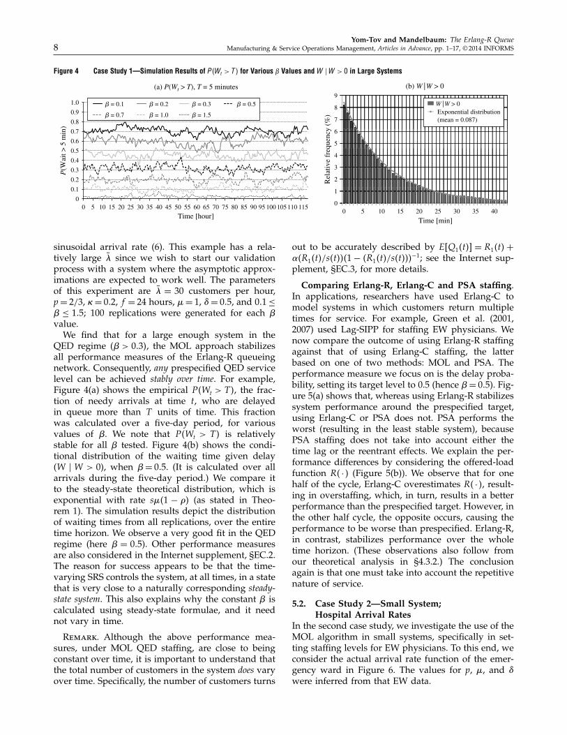
Figure 4 Case Study 1—Simulation Results of P 4Wt > T 5 for Various � Values and W �W > 0 in Large Systems

(a) P(Wt > T), T = 5 minutes (b) W |W > 0

00 5 10 15 20 25 30 35 40

00

1

2

3

4

5

6

Rel

ativ

e fr

eque

ncy

(%)

7

8

9

5 10 15 20 25

Time [min]Time [hour]

30 35 4045 50

0.1

0.2

0.3

0.4

0.5

0.6

P(W

ait >

5 m

in)

0.7

0.8

0.9

1.0

55 60 65 70 75 80 85 90 95 100 105 110 115

� = 0.1 � = 0.2 � = 0.3 � = 0.5

� = 0.7 � = 1.0 � = 1.5

W |W > 0Exponential distribution(mean = 0.087)

sinusoidal arrival rate (6). This example has a rela-tively large �̄ since we wish to start our validationprocess with a system where the asymptotic approx-imations are expected to work well. The parametersof this experiment are �̄ = 30 customers per hour,p = 2/3, �= 002, f = 24 hours, �= 1, �= 005, and 001 ≤

� ≤ 105; 100 replications were generated for each �value.

We find that for a large enough system in theQED regime 4� > 0035, the MOL approach stabilizesall performance measures of the Erlang-R queueingnetwork. Consequently, any prespecified QED servicelevel can be achieved stably over time. For example,Figure 4(a) shows the empirical P4Wt > T 5, the frac-tion of needy arrivals at time t, who are delayedin queue more than T units of time. This fractionwas calculated over a five-day period, for variousvalues of �. We note that P4Wt > T 5 is relativelystable for all � tested. Figure 4(b) shows the condi-tional distribution of the waiting time given delay(W � W > 0), when �= 005. (It is calculated over allarrivals during the five-day period.) We compare itto the steady-state theoretical distribution, which isexponential with rate s�41 − �5 (as stated in Theo-rem 1). The simulation results depict the distributionof waiting times from all replications, over the entiretime horizon. We observe a very good fit in the QEDregime (here � = 005). Other performance measuresare also considered in the Internet supplement, §EC.2.The reason for success appears to be that the time-varying SRS controls the system, at all times, in a statethat is very close to a naturally corresponding steady-state system. This also explains why the constant � iscalculated using steady-state formulae, and it neednot vary in time.

Remark. Although the above performance mea-sures, under MOL QED staffing, are close to beingconstant over time, it is important to understand thatthe total number of customers in the system does varyover time. Specifically, the number of customers turns

out to be accurately described by E6Q14t57 = R14t5 +

�4R14t5/s4t5541 − 4R14t5/s4t555−1; see the Internet sup-

plement, §EC.3, for more details.

Comparing Erlang-R, Erlang-C and PSA staffing.In applications, researchers have used Erlang-C tomodel systems in which customers return multipletimes for service. For example, Green et al. (2001,2007) used Lag-SIPP for staffing EW physicians. Wenow compare the outcome of using Erlang-R staffingagainst that of using Erlang-C staffing, the latterbased on one of two methods: MOL and PSA. Theperformance measure we focus on is the delay proba-bility, setting its target level to 0.5 (hence �= 005). Fig-ure 5(a) shows that, whereas using Erlang-R stabilizessystem performance around the prespecified target,using Erlang-C or PSA does not. PSA performs theworst (resulting in the least stable system), becausePSA staffing does not take into account either thetime lag or the reentrant effects. We explain the per-formance differences by considering the offered-loadfunction R4 · 5 (Figure 5(b)). We observe that for onehalf of the cycle, Erlang-C overestimates R4 · 5, result-ing in overstaffing, which, in turn, results in a betterperformance than the prespecified target. However, inthe other half cycle, the opposite occurs, causing theperformance to be worse than prespecified. Erlang-R,in contrast, stabilizes performance over the wholetime horizon. (These observations also follow fromour theoretical analysis in §4.3.2.) The conclusionagain is that one must take into account the repetitivenature of service.

5.2. Case Study 2—Small System;Hospital Arrival Rates

In the second case study, we investigate the use of theMOL algorithm in small systems, specifically in set-ting staffing levels for EW physicians. To this end, weconsider the actual arrival rate function of the emer-gency ward in Figure 6. The values for p, �, and �were inferred from that EW data.


Figure 5 Case Study 1—Comparing Erlang-R, Erlang-C, and PSA

(a) P(Wt > 0) (b) R(t)

R(t

)

00

0.1

0.2

0.3

0.4

0.5

0.6

P(W

> 0

)

0.7

0.8

0.9

1.0

20 40 60

Erlang-RErlang-CPSAArrival rate

80 100 120

Time [hour] Time [hour]

140 160 180 200 220 240

0.65

0.60

0.55

0.50

Arr

ival

rat

e

0.45

0.40

0.35

105

110

100

95

90

85

80

75

700 1 2 3 4 5 6 7 8 9 10 11 12 13 14 15 16 17 18 19 20 21 22 23

Erlang-R Erlang-C PSA

There are obvious problems in applying our MOLapproach to small systems: First, our approxima-tions are expected to be less accurate, being limitsas systems grow indefinitely. (In our simulation, thenumber of servers changes between one and eight.)Second, rounding up a “theoretical” need of say1.5 servers to two servers means adding 30% excesscapacity to the required capacity, which suggests dif-ficulties in stabilizing performance around prespeci-fied values. Related to this is the fact that the set ofachievable performance measures is manifestly dis-crete for small systems: changing the staffing level of asmall system by a single server could discontinuouslychange its performance. For example, if the offered-load is R = 2075, the values that P4W > 05 can haveare shown in Table 1. Finally, one cannot have an EWoperate with no physicians, and for small servers thislower bound of one plays a binding role. It is thereforeunclear whether, under these circumstances, we shallstill be able to stabilize system performance arounda predetermined value. Nevertheless, we found thatit is possible to stabilize even such small systems,given specific (though not all, as expected) targetperformance levels. The performance measures are

Figure 6 Case Study 2—Plot of Arrival Rates in an Emergency Ward

16

18

12

14

8

10

4

6

Patie

nts

per

hour

0

2

0 1 2 3 4 5 6 7 8 9 10 11 12 13 14 15 16 17 18 19 20 21 22 23

Hour of day

relatively stable, and the four possible scenarios arevisibly separable. (Because of space limitations, wehave not included supporting graphs; furthermore,Figure 9(a) in §6 well demonstrates these phenomenain an even more complex environment.)

There is another important impact of system sizethat we observed in this case study. When verifyingwhether the relation between actual P4W > 05 and �fits the Halfin–Whitt formula, we note a gap betweenthe two (see the left diagram in Figure 7). The left plotin Figure 7 shows the relationship between these func-tions, when we consider the target � values used inthe square-root formula. In most cases, the empiricalfunction is shifted downward, and the gap betweenthe two is reduced as � grows. This is mainly dueto the rounding procedure. The right plot of Figure 7shows the same graph, but as a function of the effec-tive � values. We observe that the two functions havethe same shape but the empirical function is shiftedupward. The gap between them appears to be con-stant. As this seems to be the effect of using asymp-totic approximations in such a small system, we alsoapplied the refined approximations of Janssen et al.(2011). This caused the gap to narrow, but it is stillnoticeable.

The practical guideline that can be derived fromthese graphs is that, when targeting a specificP4W > 05 value, one should use a smaller value of �,

Table 1 Small Systems: An Example of a Discrete Range forP 4W > 05, as a Function of �

Target � range Effective � s P 4W > 05 (%)

4004741100557 1.055 4 34004100551106587 1.658 5 11044106581202617 2.261 6 3001.658 and up � 7 0

Note. We distinguish between target � and effective �; the latter is the �

actually used, calculated by 4�= 4�s� −R15/√

R15.


Figure 7 Case Study 2—Comparison of the Erlang-R Simulation to the Formulae in Halfin and Whitt (1981) and Janssen et al. (2011)

0 0.2 0.4 0.6 0.8 1.0 1.2 1.4 1.6 1.8 2.0

0.4

0.5

0.6

0.7

0.8

0.9

1.0

0

0.1

0.2

0.3

P(W

> 0

)

� (effective)

EmpiricalJanssen et al.

0.4

0.5

0.6

0.7

0.8

0.9

1.0

0

0.1

0.2

0.3

0 0.2 0.4 0.6 0.8

� (target)1.0 1.2 1.4 1.6

P(W

> 0

)

Empirical

Halfin–Whitt Halfin–Whitt

based on the left diagram of Figure 7. More researchis also needed to understand the Halfin–Whitt (andJanssen et al. 2011) function for small systems whilealso considering the rounding effect. As a first step,one can develop graphs such as Figure 7, using asteady-state simulation of an Erlang-C model.

6. Using Erlang-R for Staffing EWPhysicians: Fitting a Simple Modelto a Complex Reality

In this last case study, we test Erlang-R as a sup-port tool for planning a real system. Specifically, wedemonstrate that it can be used to practically planstaffing of physicians in an EW, although the realsystem is far more complicated than our model. Inpassing, we show that applying Erlang-C to the realsystem is inferior to Erlang-R. The EW system wasbriefly described in our introduction; for a completedescription see Marmor and Sinreich (2005). In ourexperiment, we use their accurate and detailed EWsimulation model (it takes into account even walkingdistances), which is flexible in that it is easily adaptedto a given EW. We fit the simulator to the EW of ourpartner Israeli hospital (Armony et al. 2011), and thenuse the simulator as an accurate portrait of the com-plex EW reality.

Clearly, many of our main assumptions do not holdin the EW environment. For example, service timesare not exponentially distributed and could dependon the load in the EW, as follows from Armony et al.(2011). Moreover, there are seven types of patients thatseek EW services, and each type goes through a differ-ent routing process during their sojourn. The physi-cians are divided into four groups, according to theirexpertise. There is an explicit connection between apatient type and a physician group. We now sim-plify this complex system into an Erlang-R by setting

parameter values, for each physician type separately,as follows:

• Arrival rate: �4 · 5 is the average arrival rate foreach hour of the day, for each physician group, asshown in Figure 8.

• Needy times: E6S17= 1/� is estimated by averag-ing all services given by a specific physician group.

• Content times: E6S27 = 1/� is the average timebetween successive visits of a patient to the physician.

• Probability of returning to the physician for anadditional service: p is deduced from the averagenumber of visits of patients to their physician, whichwe take to be 1/41 − p5 and solve for p.

Table 2 specifies the estimated parameters accord-ing to physician type. We calculated (simply via aspreadsheet) the offered-load using the differentialEquations (3), and ran the staffing recommendationwith our EW simulation. We assumed that changesin staffing could be implemented in a one-hour res-olution. For each interval, we calculated the averagenumber of physicians needed and rounded up to thenearest integer. We used one replication of 100 weeks.(The first setup week was excluded.)

Figure 8 shows the arrival rate and the recom-mended number of physicians during the day, foreach type of physician, with � = 005. The number ofphysicians varies between one and four. We observethat the staffing function lags behind the arrival ratefunction, with an approximate time lag of two hours.Note that the number of physicians does not change

Table 2 Emergency Ward Simulation Parameters

Physician Patienttype type � E6S17 [hour] � E6S27 [hour] p

1 1, 7 8091 0.112 0.953 1.049 0.77432 2, 5 8086 0.113 0.969 1.031 0.60943 3, 6 10033 0.097 0.572 1.749 0.64414 4 12037 0.081 1.310 0.763 0.7268


Figure 8 Emergency Ward Case Study—Patient Arrivals and Physician Staffing for Each Physician Type in Emergency Ward Simulation 4�= 0055

0

1

2

3

4

5

0

1

2

3

4

5

6

7

0 1 2 3 4 5 6 7 8 9 10 11 12 13 14 15 16 17 18 19 20 21 22 23 24

Num

ber

of d

octo

rs

Arr

ival

rat

e

Time [hour]

Arrivals patient type 1 + 7



Arrivals patient type 4

Staffing doctors type 1




every hour, and natural shift schedules could bederived to fit this graph.

This EW system is small with merely a few“servers.” Our results are summarized in Figure 9(a),which depicts the probability of waiting for four val-ues of beta: 0.1, 0.5, 1.0, and 1.5; the four casesare clearly separable and become more stable as �increases. Figure 9(b) shows a comparison betweenthe results of Erlang-R and Erlang-C for � = 105,which is the easiest case to stabilize since the numberof physicians is the largest. We clearly observe thesignificant difference between the results of the twostaffing procedures, where Erlang-R yields a muchmore stable performance. Table 3 completes the pic-ture by presenting the residual mean square error(RMSE) and average percentage error (APE) foreach � category and patient–physician combination.A smaller value of these measures indicates a morestable performance. We see that Erlang-R is superior

Figure 9 Emergency Ward Case Study—P 4Wt > 05 for Various � Values

(a) Erlang-R (b) Erlang-C vs. Erlang-R (� = 1.5)1.0

0.9

0.8

0.7

0.6

0.5

P(W

> 0

)

0.4

0.3

0.2

0.1

00 24 48

� = 0.1 � = 0.5 � = 1.0 � = 1.5

72

Time in week [hour]96 120 144

0.6

P(W

> 0

)

00

0.1

0.2

0.3

0.4

0.5

24 48 72

Time in week [hour]96 120 144

Erlang-C Erlang-R

across all � values and all physician types, but thatthe variability (when � = 005) is higher at the patientlevel than the aggregated one. This is mainly becausesome of the patient types have very small demandand therefore hit the staffing constraints more oftenthan others. As � grows, this difference diminishes.(Supporting figures are omitted for lack of space.) Wealso observe that Erlang-R improves stability by 20%–350% (depending on � and patient-type), which couldbe very significant.

To conclude, despite the simplicity of the Erlang-Rmodel, it does manage to capture the importantaspects of patient visits in the EW, and hospital man-agement can use it to calculate recommended staffingfor physicians. The same outcome can be expected fornurse staffing. In fact, one would expect better resultsfor nurse staffing since it gives rise to a higher numberof servers, hence the MOL is likely to be more accurate.


Table 3 Stability Comparison Between Erlang-R and Erlang-C Staffingin an Emergency Ward

(a) P 4Wt > 05 by � (b) P 4Wt > 05 by physician type (�= 005)

PhysicianModel � RMSE APE Model type RMSE APE

Erlang-R 0.1 0.091 0.348 Erlang-R 1 0.105 0.2170.5 0.058 0.338 2 0.142 0.4591 0.061 0.410 3 0.109 0.2591.5 0.031 0.404 4 0.115 0.289

Erlang-C 0.1 0.113 0.397 Erlang-C 1 0.185 0.3840.5 0.131 0.499 2 0.139 0.4801 0.118 0.588 3 0.133 0.3241.5 0.111 0.688 4 0.162 0.436

Notes. RMSE =√

4∑n

t=14�s4t5− �e525/n, APE = 41/n5

∑nt=1 �4�s4t5 − �e5/

�e�, where �s4t5 is the simulated probability of waiting at time interval t and�e is the stable theoretical value the system was designed to achieve. (Herethe time interval is one hour, measured over a week, namely, n = 167.)

7. Fluid and Diffusion Modelsof the Number of NeedyCustomers, with Applicationto Mass Casualty Events

In this section, we develop fluid and diffusion lim-its for Erlang-R. We then use the resulting models/approximations to analyze an MCE, in which servicedemand fluctuates significantly and exceeds capac-ity, over a relatively short time period. Note thatfluid models are naturally useful for analyzing time-varying systems, and they are also useful towardunderstanding the finite-horizon evolution of systemsin a steady state. For example, one might seek toevaluate the probability that the number of customers(patients) in the system exceeds a certain thresholdduring a specific time horizon. This could support thedesign of alarm protocols such as when to commencespecial procedures: ambulance diversion or summon-ing additional medical staff. In designing such proto-cols, for example, toward avoiding excessive alarms,one would in fact require our diffusion refinementsthat determine confidence intervals around fluid sam-ple paths; see Mandelbaum et al. (1999).

It was already noted that Erlang-R, both sta-tionary and time varying, fits the mathematicalframework of Markovian service networks in Man-delbaum et al. (1998). This framework justifies theexistence and uniqueness of model solutions thataccommodate time-varying arrivals and time-varyingstaffing policies. Specifically, Erlang-R is representedby Q = 8Q4t51 t ≥ 09, Q4t5= 4Q14t51Q24t55: Q14t5 is thenumber of needy patients in the system at time t (i.e.,those either waiting for service or being served), andQ24t5 is the number of content patients in the sys-tem. The process Q is characterized by the following

sample-path equations, for t ≥ 0:

Q14t5 = Q1405+Aa1

(

∫ t

0�u du

)

−Ad2

(

∫ t

0p�4Q14u5∧su5du

)

−A12

(

∫ t

041−p5�4Q14u5∧su5du

)

+A21

(

∫ t

0�Q24u5du

)

1

Q24t5 = Q2405+A12

(

∫ t

0p�4Q14u5∧su5du

)

−A21

(

∫ t

0�Q24u5du

)

1

where Aa1, Ad

2 , A12, and A21 are four mutually inde-pendent time-homogeneous Poisson processes withrate 1. We now introduce a family of scaled queue-ing models, indexed by � ↗ �, such that both thearrival rate and the number of physicians are scaledup by �, and the needy and content service ratesremain unscaled:

Q�1 4t5=Q�

1 405+Aa1

(

∫ t

0��u du

)

−Ad2

(

∫ t

0�p�

(

1�Q�

1 4u5∧ su

)

du

)

−A12

(

∫ t

0�41 − p5�

(

1�Q�

1 4u5∧ su

)

du

)

+A21

(

∫ t

0��

(

1�Q�

2 4u5

)

du

)

1

Q�2 4t5=Q�

2 405+A12

(

∫ t

0�p�

(

1�Q�

1 4u5∧ su

)

du

)

−A21

(

∫ t

0��

(

1�Q�

2 4u5

)

du

)

0

(11)

Theorem 6. (FSLLN) Through the scaling (11), wehave

lim�→�

Q�4t5

�=Q4054t51 t ≥ 01

where Q4054 · 5, the fluid approximation/model, is the solu-tion of the following ODE:

Q4051 4t5=Q

4051 405

+

∫ t

04�u −�4Q

4051 4u5∧ su5+ �Q

4052 4u55 du1

Q4052 4t5=Q

4052 405

+

∫ t

04p�4Q

4051 4u5∧ su5− �Q

4052 4u55 du0

(12)

The convergence to Q4054 · 5 is almost surely uniformly oncompacts.

The theorem follows from Theorem 2.2 in Mandel-baum et al. (1998). We continue by developing diffu-sion approximations for Erlang-R. These are used for


calculating variances and covariances, which, in turn,yield confidence intervals for the number of patientsin the system.

Theorem 7. (FCLT) Through the scaling (11) and withthe fluid limits (12), we have

lim�→�

√�

[

Q�4t5

�−Q4054t5

]

d=Q4154t51 t ≥ 01 (13)

where Q4154 · 5, the diffusion model/approximation, is thesolution of a stochastic differential equation, as given by(EC.9) in the Internet supplement, §EC.1.6. The conver-gence to Q4154 · 5 is the standard Skorohod J1 convergencein D601�5.

The theorem is a consequence of Theorem 2.3 inMandelbaum et al. (1998). Our fluid and diffusionmodels are easiest to apply when durations of criticalloading are negligible (the zero-measure assumptionin Mandelbaum et al. 2002). They are thus naturalas models for MCEs, during which overloading con-stantly prevails. Formally, we have the following:

Proposition 2. Define S to be the set of times whenthe fluid number of physicians equals the number ofpatients in the needy state: S = 8t > 0 � Q

4051 4t5 = st9.

Assume that this set of times S has measure zero. Then(EC.9) simplifies to

Q4151 4t5 = Q

4151 405

+

∫ t

04−�1

8Q4051 4u5≤su9

Q4151 4u5+ �Q

4152 4u55 du

+Ba1

(

∫ t

0�u du

)

−Bd2

(

∫ t

0p�4Q

4051 4u5∧ su5 du

)

−B12

(

∫ t

041 − p5�4Q

4051 4u5∧ su5 du

)

+B21

(

∫ t

0�Q

4052 4u5du

)

1 (14)

Q4152 4t5 = Q

4152 405

+

∫ t

04p�1

8Q4051 4u5≤su9

Q4151 4u5− �Q

4152 4u55 du

+B12

(

∫ t

0p�4Q

4051 4u5∧ su5 du

)

−B21

(

∫ t

0�Q

4052 4u5du

)

0

The mean vector for the diffusion approximation (EC.10)is then

d

dtE6Q

4151 4t57= −�1

8Q4051 4t5≤st9

E6Q4151 4t57+ �E6Q

4152 4t571

d

dtE6Q

4152 4t57= p�1

8Q4051 4t5≤st9

E6Q4151 4t57− �E6Q

4152 4t573

and the covariance matrix (EC.11) is

d

dtVar6Q415

1 4t57

=−2�18Q

4051 4t5≤st9

Var6Q4151 4t57+2�Cov6Q415

1 4t51Q4152 4t57

+�t+�Q4052 4t5+�4Q

4051 4t5∧st51

d

dtVar6Q415

2 4t57

=−2�Var6Q4152 4t57+2p�Cov6Q415

1 4t51Q4152 4t57

+p�4Q4051 4t5∧st5+�Q

4052 4t51

d

dtCov6Q415

1 4t51Q4152 4t57

=−4�18Q

4051 4t5≤st9

+�5Cov6Q4151 4t51Q

4152 4t57

+�Var6Q4152 4t57+p�1

8Q4051 4t5≤st9

Var6Q4151 4t57

−p�4Q4051 4t5∧st5−�Q

4052 4t50

(15)

Proposition 2 supports MCE modeling and man-agement, which we turn to next.

7.1. Mass Casualty EventsWhen an MCE is in progress, the EW must, over ashort time period, attend to already admitted patients,release those who can be released, and most impor-tantly, provide emergency care to new arrivals atovercapacity rates. We now demonstrate that ourtransient fluid and diffusion models, from the previ-ous subsection, usefully capture the state of an EWduring an MCE. This enables one to use Erlang-R foroff-line planning of an MCE, initial reaction at its out-set (customized to the MCE type, severity and scale),and subsequently online MCE control until the eventwinds up. We focus as before on staffing. To this end,we use data from a chemical MCE drill. The MCEtook place in July 2010 at 11:00 a.m. and lasted till13:15; its casualties were transported to an Israeli hos-pital where our data were collected. The short horizonof MCEs (here two hours) and the protocol of chemi-cal events (periodic treatment of patients) renders thetransient Erlang-R, with its recurrent service structure,naturally appropriate.

Our data is for the severely wounded nontraumapatients. Figure 10(a) depicts cumulative arrival anddeparture counts, collected roughly during 11:15–13:15. The arrival rate is clearly time varying: peri-ods with no arrivals alternate with approximatelyconstant arrival rates, with the rates decreasing astime progresses. (Our hospital partners, experiencedin managing MCEs, inform us that this piecewise-constant pattern of arrival rate is typical of MCEs:it is attributed to the fact that casualties are trans-ported from the MCE scene by a finite number of


Figure 10 Chemical Mass Casualty Event Drill: Arrivals, Departures, and Erlang-R Approximations

(a) Arrival and departures in MCE drill (b) Erlang-R approximations (fluid and diffusion)

11:020

10

20

30

40

50

Tot

al n

umbe

r of

pat

ient

s

60 30

25

20

15

10

5

0

Actual Q(t)Fluid Q(t)

Fluid Q1

Lower envelope Q(t) (theoretical)Upper envelope Q(t) (theoretical)

Cumulative arrivals

Cumulative departures

11:16 11:31 11:45 12:00 12:14

Time [hour:min]12:28 12:43 12:57 13:12 13:26 11:02 11:16 11:31 11:45 12:00 12:14

Time [hour:min]12:28 12:43 12:57 13:12 13:26

ambulances, who traverse back and forth.) The esti-mated arrival rate function (customers per minute) isas follows (16a1b5 is an indicator function):

�t = 00773 × 16012254t5+ 00884 × 164416954t5

+ 005 × 16102111754t51 0 ≤ t ≤ 1200 (16)

Erlang-R parameters were estimated from medi-cal specifications and the physics of Erlang-R, as wenow explain. The severity level of the patients underconsideration calls for medication every 30 minutes,in addition to treating their injuries. Staffing specsassigned every physician to four patients at a time.(In reality, and being a drill, there were ample physi-cians on site, which implies, no upper bound on thenumber of physicians (s = �). Such resource levelsare unlikely to prevail in true-to-life MCEs, but theyfacilitate the estimation of parameter values—whichare practice relevant.) One can now estimate �, p, �via the following three equations:

1/�+ 1/�= 303 1/�+ 30p/41 − p5= 62043

�/�= 3/p0(17)

The first equation corresponds to the 30-minutecycle. The second represents length of stay (LOS) asthe first service followed by a geometric number ofcycles; the average LOS of 62.4 minutes is then theclassical Kaplan–Meier estimator (Kaplan and Meier1958) for censored data: indeed, patients that werestill in treatment when the drill ended (about 20out of 50) provided only lower bounds on their LOS.The last equation arises from the patients-to-physicianratio 4R1 +R25/4 =R1, in which R1, R2 are the steady-state offered-loads from §3. Solving the equationsin (17) yields average treatment time of 5.4 min-utes (�= 11006), average content time 24.6 minutes(�= 2044) and p = 00662.

We now compare, in Figure 10(b), Erlang-R esti-mators against MCE data. First we have fluid-basedestimators for Q =Q1 +Q2, the total number of casu-alties, enveloped by a diffusion-based 95% confidenceband. This is to be compared against the actual sam-ple path, observed from our MCE data (the differ-ence between cumulative arrivals and departures).Erlang-R clearly captures well the transient nature ofthe MCE: the data is essentially within its confidenceband. Notably, a comparison (omitted for space con-straints) of Erlang-R with Erlang-C demonstrated thatthe latter yields noticeably inferior path-estimators: anincrease of about 45% in RMSE and APE measures,for the reasons that were explained in §4.3.2.

After validating Erlang-R against the observed Q,one can now trust it to infer the number of busyphysicians—see the dashed function Q1 in Fig-ure 10(b). Its evolution was unobservable at the MCEdrill, which is a state of affairs that is to be commonlyexpected. Yet Q1 is essential for planning and controlof MCEs, as discussed next.

7.1.1. Erlang-R in Support of MCE Staffing.Since Erlang-R reliably captures MCE dynamics, onecan use it to support planning for an MCE, initialreaction to its severity and scale and, ultimately, con-trolling MCE evolution. For concreteness we considerstaffing upon initial reaction. The procedure wouldbe similar in planning, when applying Erlang-R forcomparative analysis of plausible scenarios, and con-trol, where parameter values are updated adaptivelyand then fed into Erlang-R over a rolling horizon. Allthese applications entail the following steps:

1. Forecasting the arrival rate function �t (e.g., (16))for each severity group of patients. Any forecastingmodel should take into account the estimated num-ber of casualties routed to the hospital, number of


ambulances available, and distance from the hospital(Jacobson et al. 2012).

2. Estimating the offered-load R4 · 5 for each severitygroup, taking into account group-specific treatmentprotocols as demonstrated above.

3. Calculating the staffing function s4 · 5 via s4t5 =

6R4t5 + �√

R4t57, t ≥ 0. We recommend a relativelyhigh �, say � ≥ 2, to account for the emergency sit-uation at hand. One should then accommodate con-straints such as the available number of physicianswithin the hospital and the availability and time-to-arrive of out-of-hospital physicians.

4. Predicting EW evolution via Erlang-R under theplanned SRS.

Given our RFID-based data in Figure 10, we nowdemonstrate the above steps by planning for staffingan MCE. Being able to infer Q1 (Figure 10) yieldsinsights that exploit its special structure of threephases: a first surge of arrivals (11:00–12:00), peakperiod (12:00–13:00), and a closure phase from 13:00till completion; each phase starts with an increase ofload, which is immediately followed by a decreasebecause of ambulances returning to the MCE scene.As will be demonstrated, this allows one to initiallydivert physicians within the hospital to cater to thefirst surge while, in parallel, summon off-duty staffwho would join (say from home) toward the secondpeak surge. Staffing remains constant within a phase,which gives rise to the following plan:

1. Initial reaction: Recall that the MCE occurred at11:00. The first casualties arrived to the hospital at11:15, thus starting a surge of demand (offered-load)that peaks at 11:40: Q1 = 5. By SRS, this calls for 5 +

2√

5 ≈ 9 physicians, which are to arrive, conceivablyfrom the hospital itself, until 11:15.

2. Peak period: From 12:07, demand for physiciansincreases to a peak Q1 = 705 at 12:25. One needs now705+2

√705 ≈ 13 physicians, or an additional group of

four physicians that can join within hour from MCEstart.

3. Closure: This last phase starts around 13:00, andarrivals cease at 13:15. A real MCE would continue atthe hospital till all casualties are hospitalized, whilegradually releasing physicians to their routine or reas-signing them to help with already-hospitalized casu-alties. Similarly to the above (not pursued here), onecan again use Erlang-R to plan for the release ofphysicians, which, interestingly, involves also the pre-diction of the MCE completion time.

As mentioned, Chemical MCEs naturally fit therecurrent service structure of Erlang-R. Other typesof MCEs might need other models. For example,with relatively more trauma patients and during off-peak arrivals, physicians who perform initial lifesav-ing procedures could also accompany their patientsthrough surgery. A corresponding model would then

consist of two queues in tandem, as analyzed byCohen et al. (2013).

8. Conclusions and Further ResearchMotivated by staffing applications in healthcare, wehave developed a simple-yet-not-too-simple servicemodel, Erlang-R, which accommodates returning cus-tomers in a time-varying environment. The modelvaluably captures both normal operating conditionsand MCEs. In the former, it gives rise to an explicitstaffing recipe that matches service capacity withtime-varying demand (the QED operational regime),which in turn stabilizes operational performance (ser-vice level, utilization). In MCEs the model can sup-port planning for initial reaction to and control ofsuch events.

We started, in the introduction, with four exam-ples of returning customers/patients in healthcaresystems. We can now conclude, based on the analy-sis in §§3, 4.3.2, and 7.1 and some additional hospitaldata, that Erlang-R better be used for modeling EWs(both in normal and MCE conditions) whereas, foroncology and radiology wards, Erlang-C suffices. Toelaborate, for the EW under its normal conditions,the parameters � = 002618 (as f = 24, in hours)and

√

��41 − p5 ≈ 304 are such that the EW fits theleft part of Figure 3 (in both plots). The ampli-tude ratio is within 40093100975 and the phase ratiois within 4107135, depending on patient type (seeTable 2); hence, the significant difference is betweenphases rather than amplitudes, which means thatusing Erlang-C will be mostly wrong in timing—starting (and ending) shifts too soon. In the oncologyward, the corresponding values are � = 60283 (f = 1,in days) and

√

��41 − p5= 000495. This puts oncologyon the right side of Figure 3, where we expect lit-tle if any difference between the two models. Indeed,the amplitude and phase ratios are 009987 and 009756,respectively, namely, very close to unity. Next, radi-ology operates in a steady-state environment, sincethe arrival rate is constant, and thus need not useErlang-R. Finally, our last example, EW under MCEstress, must be modeled as Erlang-R since, in tran-sient times (over a short time horizon), the differencebetween Erlang-R and Erlang-C is significant.

It is important to emphasize that, even in thecase when Erlang-C suffices to capture overall per-formance, Erlang-R would still be preferable over afinite horizon, or for focusing on the performanceof needy (content) patients. Erlang-R is also capableof capturing usefully, as in §6, the operational per-formance of a full-scale EW, from the point of viewof its physicians: the model plainly aggregates the“world beyond physicians” into a single ample-serverstation. One could do the same with EW nurses.


One could also raise the more general question ofapproximating a general queueing network, from thepoint of a specific node, by an Erlang-R model (thespecific node would be needy while the rest of thenetwork is content)—when do such crude approxima-tions work and, alternatively, when are their refine-ments necessary?

The healthcare environment suggests further exten-sions for Erlang-R. To name a few, Yom-Tov (2010)adds an upper bound on the overall number of cus-tomers in the system, which corresponds to finite bedcapacity; Chan et al. (2014) consider state-dependentservice times; Huang et al. (2012) trade off high pri-ority to patients on their first visit versus, alterna-tively, to those who have been in the system for a longtime; and, finally, customer abandonment can takeplace during a first waiting (left without being seen)or between services (left against medical advice). Weconclude with an outstanding open theoretical prob-lem, which is the analysis of the limiting time-varyingdiffusion process under SRS. This is a prerequisite forunderstanding the success of our time-varying MOLstaffing.

Supplemental MaterialSupplemental material to this paper is available at http://dx.doi.org/10.1287/msom.2013.0474.

AcknowledgmentsThe authors thank Yariv Marmor for providing them accessto his EW simulator. The work of Avishai Mandelbaumwas partially supported by the United States–Israel Bina-tional Science Foundation [Grants 2005175, 2008480]; theIsrael Science Foundation [Grant 1357/08]; and by theTechnion funds for promotion of research and sponsoredresearch. Some of the research was funded by and carriedout while Avishai Mandelbaum was visiting the Statisticsand Applied Mathematical Sciences Institute of the NationalScience Foundation; the Department of Statistics and Oper-ations Research, the University of North Carolina at ChapelHill; the Department of Information, Operations and Man-agement Sciences, Leonard N. Stern School of Business,New York University; and the Department of Statistics, theWharton School, University of Pennsylvania—the wonder-ful hospitality of these institutions is gratefully acknowl-edged and truly appreciated. The work of Galit Yom-Tovwas partially supported by the Israel National Institute forHealth Policy and Health Services Research.

ReferencesArmony M, Israelit S, Mandelbaum A, Marmor YN, Tseytlin Y,

Yom-Tov GB (2011) Patient flow in hospitals: A data-basedqueueing-science perspective. Working paper, Technion–IsraelInstitute of Technology, Technion City, Haifa. http://iew3.technion.ac.il/serveng/References/references.

Borst S, Mandelbaum A, Reiman M (2004) Dimensioning large callcenters. Oper. Res. 52(1):17–34.

Chan CW, Yom-Tov GB, Escobar G (2014) When to use speedup:An examination of service systems with returns. Oper. Res.Forthcoming.

Cohen I, Mandelbaum A, Zychlinski N (2013) Minimizing mortalityin a mass casualty event: Fluid networks in support of mod-eling and staffing. IIE Trans., ePub ahead of print October 30,http://dx.doi.org/10.1080/0740817X.2013.855846.

Eick SG, Massey WA, Whitt W (1993a) Mt/G/� queues with sinu-soidal arrival rates. Management Sci. 39(2):241–252.

Eick SG, Massey WA, Whitt W (1993b) The physics of the Mt/G/�queue. Oper. Res. 41(4):731–742.

Falin GI, Templeton JGC (1997) Retrial Queues (Chapman & Hall,London).

Feldman Z, Mandelbaum A, Massey WA, Whitt W (2008) Staffing oftime-varying queues to achieve time-stable performance. Man-agement Sci. 54(2):324–338.

Gans N, Koole G, Mandelbaum A (2003) Telephone call centers:A tutorial and literature review. Manufacturing Service Oper.Management 5(2):79–141.

Green L, Kolesar PJ, Soares J (2001) Improving the SIPP approachfor staffing service systems that have cyclic demands. Oper.Res. 49(4):549–564.

Green L, Kolesar PJ, Whitt W (2007) Coping with time-varyingdemand when setting staffing requirements for a service sys-tem. Production Oper. Management 16(1):13–39.

Green L, Soares J, Giglio JF, Green RA (2006) Using queuing theoryto increase the effectiveness of emergency department providerstaffing. Academic Emergency Medicine 13(1):61–68.

Halfin S, Whitt W (1981) Heavy-traffic limits for queues with manyexponential servers. Oper. Res. 29:567–587.

Huang J, Carmeli B, Mandelbaum A (2012) Control of patient flowin emergency departments, or multiclass queues with dead-lines and feedback. Working paper, Technion–Israel Institute ofTechnology, Technion City, Haifa.

Israel Ministry of Health (2006) Financial report for years 2000–2005. Report, Israel Ministry of Health, Jerusalem. http://www.health.gov.il/publicationsFiles/finance2005.pdf.

Jacobson EU, Argon NT, Ziya S (2012) Priority assignment in emer-gency response. Oper. Res. 60(4):813–832.

Janssen AJEM, van Leeuwaarden JSH, Zwart B (2011) Refiningsquare-root safety staffing by expanding Erlang C. Oper. Res.59(6):1512–1522.

Jennings O, Mandelbaum A, Massey W, Whitt W (1996) Serverstaffing to meet time-varying demand. Management Sci.42(10):1383–1394.

Jennings OB, de Véricourt F (2011) Nurse staffing in medical units:A queueing perspective. Oper. Res. 59(6):1320–1331.

Kaplan EL, Meier P (1958) Nonparametric estimation from incom-plete observations. J. Amer. Statist. Assoc. 53(282):457–481.

Khudyakov P, Gorfine M, Feigin P (2010) Test for equality of base-line hazard functions for correlated survival data using frailtymodels. Working paper, Technion–Israel Institute of Technol-ogy, Technion City, Haifa.

Lahiri A, Seidmann A (2009) Analyzing the differential impactof radiology information systems across radiology modalities.J. Amer. College of Radiology 6(10):522–526.

Maman S (2009) Uncertainty in the demand for service: The caseof call centers and emergency departments. Master’s thesis,Technion–Israel Institute of Technology, Technion City, Haifa.

Mandelbaum A, Massey W, Reiman M (1998) Strong approxi-mations for Markovian service networks. Queueing Systems30(1–2):149–201.

Mandelbaum A, Massey WA, Reiman M, Rider B (1999) Time vary-ing multiserver queues with abandonment and retrials. Key P,Smith D, eds. ITC-16, Teletraffic Engineering in a CompetitiveWorld (Elsevier), 355–364.

Mandelbaum A, Massey WA, Reiman M, Stolyar A, Rider B (2002)Queue lengths and waiting times for multiserver queues withabandonment and retrials. Telecomm. Systems 21(2–4):149–171.


Marmor Y, Sinreich DA (2005) Emergency department operations:The basis for developing a simulation tool. IIE Trans. 37(3):233–245.

Massey WA, Whitt W (1993) Networks of infinite-server queueswith nonstationary Poisson input. Queueing Systems 13(1):183–250.

Massey W, Whitt W (1994) An analysis of the modified offered-loadapproximation for the nonstationary Erlang loss model. Ann.Appl. Probab. 4(4):1145–1160.

Whitt W (2007) What you should know about queueing models toset staffing requirements in service systems. Naval Res. Logist.55(5):476–484.

Whitt W (2013) Offered load analysis for staffing. ManufacturingService Oper. Management 15(2):166–169.

Yom-Tov G (2010) Queues in hospitals: Queueing networkswith reentering customers in the QED regime. Ph.D. thesis,Technion–Israel Institute of Technology, Technion City, Haifa.

Zeltyn S, Marmor YN, Greenshpan O, Mesika Y, Wasserkrug S,et al. (2011) Simulation-based models of emergency depart-ments: Operational, tactical, and strategic staffing. ACM Trans.Modeling Comput. Simulation (TOMACS) 21(4):Article 24.

Zhan D, Ward AR (2014) Threshold routing to trade off waitingand call resolution in call centers. Manufacturing Service Oper.Management 16(2).

erlang-r: a time-varying queue with reentrant...

Documents