erm model analysis for adaptation to hydrological model errors
TRANSCRIPT

Baymani-Nezhad, M., & Han, D. (2018). ERM model analysis for adaptationto hydrological model errors. Acta Geophysica, 66(4), 741–753.https://doi.org/10.1007/s11600-018-0137-y
Publisher's PDF, also known as Version of record
License (if available):CC BY
Link to published version (if available):10.1007/s11600-018-0137-y
Link to publication record in Explore Bristol ResearchPDF-document
This is the final published version of the article (version of record). It first appeared online via SPRINGER athttps://link.springer.com/article/10.1007%2Fs11600-018-0137-y. Please refer to any applicable terms of use ofthe publisher.
University of Bristol - Explore Bristol ResearchGeneral rights
This document is made available in accordance with publisher policies. Please cite only the publishedversion using the reference above. Full terms of use are available:http://www.bristol.ac.uk/pure/about/ebr-terms

RESEARCH ARTICLE - SPECIAL ISSUE
ERM model analysis for adaptation to hydrological model errors
M. Baymani-Nezhad1 • D. Han2
Received: 28 October 2017 / Accepted: 30 March 2018� Institute of Geophysics, Polish Academy of Sciences & Polish Academy of Sciences 2018
AbstractHydrological conditions are changed continuously and these phenomenons generate errors on flood forecasting models and
will lead to get unrealistic results. Therefore, to overcome these difficulties, a concept called model updating is proposed in
hydrological studies. Real-time model updating is one of the challenging processes in hydrological sciences and has not
been entirely solved due to lack of knowledge about the future state of the catchment under study. Basically, in terms of
flood forecasting process, errors propagated from the rainfall-runoff model are enumerated as the main source of uncer-
tainty in the forecasting model. Hence, to dominate the exciting errors, several methods have been proposed by researchers
to update the rainfall-runoff models such as parameter updating, model state updating, and correction on input data. The
current study focuses on investigations about the ability of rainfall-runoff model parameters to cope with three types of
existing errors, timing, shape and volume as the common errors in hydrological modelling. The new lumped model, the
ERM model, has been selected for this study to evaluate its parameters for its use in model updating to cope with the stated
errors. Investigation about ten events proves that the ERM model parameters can be updated to cope with the errors without
the need to recalibrate the model.
Keywords Real-time model updating � Forecasting errors � Concentration time � Time to peak
Introduction
Land use/land cover change and climate change have sig-
nificant influences on catchment hydrological characteris-
tics. The appearance of these phenomena has potential
effects on generating unusual flood events and may lead to
produce various types of flooding. Study about these nat-
ural occurrences and their interaction with hydrological
models has been mentioned in the literature with expla-
nation of methods to control and reduce their risks (Arnell
1999; Wilby et al. 1994; Xu 1999; Dibike and Coulibaly
2005; Hagg et al. 2007; Charlton et al. 2006).
Irregular rainfall events have direct linkage with unan-
ticipated floods around a catchment. Consequently, per-
forming precautionary actions like developing a model for
real-time flood warning can help reduce flood damages
during a flood event significantly. Flood forecasting is an
important part of water resource management activities
related to flood warning, flood control or reservoir opera-
tion (Yang and Michel 2000), but still lots of efforts are
required to develop highly accurate models for operational
hydrology. Real-time flood forecasting is important for
every day operation, management of water control systems
and for emergency cases where protection of life and
property is concerned (Lardet and Obled 1994). In many
countries, flood warning systems come towards the top of
the government’s policy priority list (Penning-Rowsell
et al. 2000). Accurate real-time flood forecasting with an
adequate lead time can help to confront flood hazards in an
efficient time period. Real-time flood forecasting model
and an updating technique should be integrated (Yu and
Chen 2005) which is applied by operators to predict flood
events.
All flood forecasting models are a simplification of the
reality and they simulate the flood events with errors
depending on the model structures and their adaptability
with the changes in hydrological conditions. Hence,
applying a number of efficient adaptive strategies may
& M. Baymani-Nezhad
1 Department of Civil Engineering, Karaj Branch Islamic Azad
University, Karaj, Iran
2 Water and Environmental Manager Center, University of
Bristol, Bristol, UK
123
Acta Geophysicahttps://doi.org/10.1007/s11600-018-0137-y(0123456789().,-volV)(0123456789().,-volV)
reduce model errors. Studies about flood forecasting
models can be divided into two categories: (1) developing
new models (Beven 1993; Bartholmes and Todini 2005;
Yakowitz 1985), (2) developing efficient methods to
reduce specific sources of uncertainties and improving the
current models (Brath et al. 2002; Younis et al. 2008). The
first category was studied in 2013 by Baymani-Nezhad and
Han by developing a new efficient lumped rainfall-runoff
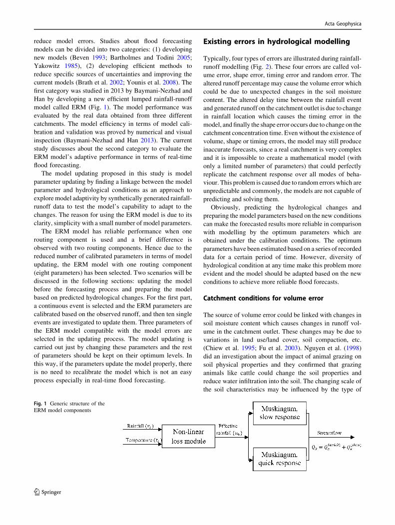
model called ERM (Fig. 1). The model performance was
evaluated by the real data obtained from three different
catchments. The model efficiency in terms of model cali-
bration and validation was proved by numerical and visual
inspection (Baymani-Nezhad and Han 2013). The current
study discusses about the second category to evaluate the
ERM model’s adaptive performance in terms of real-time
flood forecasting.
The model updating proposed in this study is model
parameter updating by finding a linkage between the model
parameter and hydrological conditions as an approach to
exploremodel adaptivity by synthetically generated rainfall-
runoff data to test the model’s capability to adapt to the
changes. The reason for using the ERM model is due to its
clarity, simplicity with a small number of model parameters.
The ERM model has reliable performance when one
routing component is used and a brief difference is
observed with two routing components. Hence due to the
reduced number of calibrated parameters in terms of model
updating, the ERM model with one routing component
(eight parameters) has been selected. Two scenarios will be
discussed in the following sections: updating the model
before the forecasting process and preparing the model
based on predicted hydrological changes. For the first part,
a continuous event is selected and the ERM parameters are
calibrated based on the observed runoff, and then ten single
events are investigated to update them. Three parameters of
the ERM model compatible with the model errors are
selected in the updating process. The model updating is
carried out just by changing these parameters and the rest
of parameters should be kept on their optimum levels. In
this way, if the parameters update the model properly, there
is no need to recalibrate the model which is not an easy
process especially in real-time flood forecasting.
Existing errors in hydrological modelling
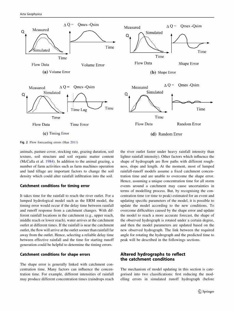
Typically, four types of errors are illustrated during rainfall-
runoff modelling (Fig. 2). These four errors are called vol-
ume error, shape error, timing error and random error. The
altered runoff percentage may cause the volume error which
could be due to unexpected changes in the soil moisture
content. The altered delay time between the rainfall event
and generated runoff on the catchment outlet is due to change
in rainfall location which causes the timing error in the
model, and finally the shape error occurs due to change on the
catchment concentration time. Even without the existence of
volume, shape or timing errors, the model may still produce
inaccurate forecasts, since a real catchment is very complex
and it is impossible to create a mathematical model (with
only a limited number of parameters) that could perfectly
replicate the catchment response over all modes of beha-
viour. This problem is caused due to random errors which are
unpredictable and commonly, the models are not capable of
predicting and solving them.
Obviously, predicting the hydrological changes and
preparing the model parameters based on the new conditions
can make the forecasted results more reliable in comparison
with modelling by the optimum parameters which are
obtained under the calibration conditions. The optimum
parameters have been estimated based on a series of recorded
data for a certain period of time. However, diversity of
hydrological condition at any time make this problem more
evident and the model should be adapted based on the new
conditions to achieve more reliable flood forecasts.
Catchment conditions for volume error
The source of volume error could be linked with changes in
soil moisture content which causes changes in runoff vol-
ume in the catchment outlet. These changes may be due to
variations in land use/land cover, soil compaction, etc.
(Chiew et al. 1995; Fu et al. 2003). Nguyen et al. (1998)
did an investigation about the impact of animal grazing on
soil physical properties and they confirmed that grazing
animals like cattle could change the soil properties and
reduce water infiltration into the soil. The changing scale of
the soil characteristics may be influenced by the type of
Fig. 1 Generic structure of the
ERM model components
Acta Geophysica
123
animals, pasture cover, stocking rate, grazing duration, soil
texture, soil structure and soil organic matter content
(McCalla et al. 1984). In addition to the animal grazing, a
number of farm activities such as farm machines operation
and land tillage are important factors to change the soil
density which could alter rainfall infiltration into the soil.
Catchment conditions for timing error
It takes time for the rainfall to reach the river outlet. For a
lumped hydrological model such as the ERM model, the
timing error would occur if the delay time between rainfall
and runoff response from a catchment changes. With dif-
ferent rainfall locations in the catchment (e.g., upper reach,
middle reach or lower reach), water arrives at the catchment
outlet at different times. If the rainfall is near the catchment
outlet, the flowwill arrive at the outlet sooner than rainfall far
away from the outlet. Hence, selecting a reliable delay time
between effective rainfall and the time for starting runoff
generation could be helpful to determine the timing errors.
Catchment conditions for shape errors
The shape error is generally linked with catchment con-
centration time. Many factors can influence the concen-
tration time. For example, different intensities of rainfall
may produce different concentration times (raindrops reach
the river outlet faster under heavy rainfall intensity than
lighter rainfall intensity). Other factors which influence the
shape of hydrograph are flow paths with different rough-
ness, slope and length. At the moment, most of lumped
rainfall-runoff models assume a fixed catchment concen-
tration time and are unable to overcome the shape error.
Hence, assuming a unique concentration time for all storm
events around a catchment may cause uncertainties in
terms of modelling process. But, by recognising the con-
centration time (or time to peak) estimated for an event and
updating specific parameters of the model, it is possible to
update the model according to the new conditions. To
overcome difficulties caused by the shape error and update
the model to reach a more accurate forecast, the shape of
the observed hydrograph is rotated under a certain degree,
and then the model parameters are updated based on the
new observed hydrograph. The link between the required
angle for rotating the hydrograph and the predicted time to
peak will be described in the followings sections.
Altered hydrographs to reflectthe catchment conditions
The mechanism of model updating in this section is cate-
gorised into two classifications: first reducing the mod-
elling errors in simulated runoff hydrograph (before
Fig. 2 Flow forecasting errors (Han 2011)
Acta Geophysica
123
forecasting) and second predicting the possible changes in
hydrological conditions and adjusting the model parame-
ters according to the new conditions. For this reason, the
observed hydrograph is changed according to the predicted
changes and the simulated hydrograph and the model
parameters are updated to simulate a runoff hydrograph
similar to the altered hydrograph. To cope with each type
of error, just one of the ERM parameters is updated.
Therefore, instead of recalibrating all of the model
parameters, the most effective parameters related to the
model errors will be updated. In some cases, the modelling
errors could be a mix of all the errors, hence it might be
required to update all the three parameters at the same time
to cope with all the sources of errors. Consequently, any
changes on the system could be carried out by just playing
with maximum three parameters. The change of the
observed hydrograph to reflect the hydrological changes
and selecting the proper parameters of the ERM model will
be described in the following sections.
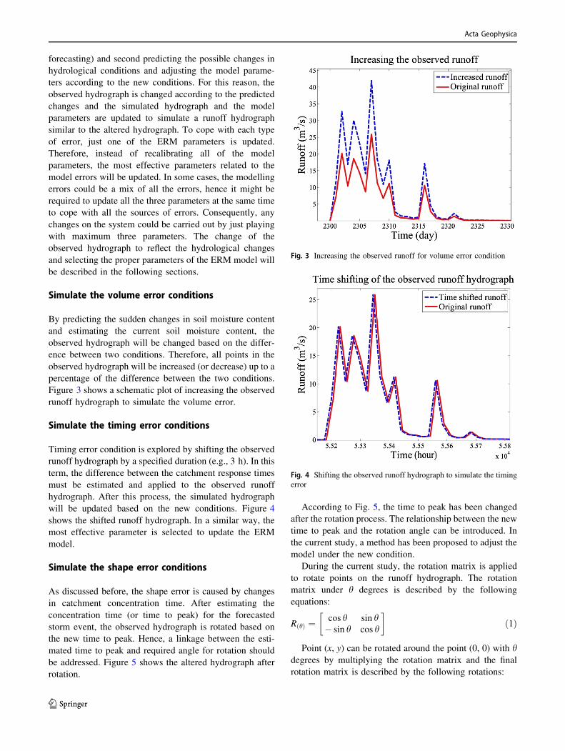
Simulate the volume error conditions
By predicting the sudden changes in soil moisture content
and estimating the current soil moisture content, the
observed hydrograph will be changed based on the differ-
ence between two conditions. Therefore, all points in the
observed hydrograph will be increased (or decrease) up to a
percentage of the difference between the two conditions.
Figure 3 shows a schematic plot of increasing the observed
runoff hydrograph to simulate the volume error.
Simulate the timing error conditions
Timing error condition is explored by shifting the observed
runoff hydrograph by a specified duration (e.g., 3 h). In this
term, the difference between the catchment response times
must be estimated and applied to the observed runoff
hydrograph. After this process, the simulated hydrograph
will be updated based on the new conditions. Figure 4
shows the shifted runoff hydrograph. In a similar way, the
most effective parameter is selected to update the ERM
model.
Simulate the shape error conditions
As discussed before, the shape error is caused by changes
in catchment concentration time. After estimating the
concentration time (or time to peak) for the forecasted
storm event, the observed hydrograph is rotated based on
the new time to peak. Hence, a linkage between the esti-
mated time to peak and required angle for rotation should
be addressed. Figure 5 shows the altered hydrograph after
rotation.
According to Fig. 5, the time to peak has been changed
after the rotation process. The relationship between the new
time to peak and the rotation angle can be introduced. In
the current study, a method has been proposed to adjust the
model under the new condition.
During the current study, the rotation matrix is applied
to rotate points on the runoff hydrograph. The rotation
matrix under h degrees is described by the following
equations:
R hð Þ ¼cos h sin h� sin h cos h
� �ð1Þ
Point (x, y) can be rotated around the point (0, 0) with hdegrees by multiplying the rotation matrix and the final
rotation matrix is described by the following rotations:
Fig. 3 Increasing the observed runoff for volume error condition
Fig. 4 Shifting the observed runoff hydrograph to simulate the timing
error
Acta Geophysica
123

xh ¼ x cos h� y sin h ! around 0; 0ð Þ ð2Þxh ¼ x0 þ ðx� x0Þ cos h� ðy� y0Þ sin h ! around x0; y0ð Þ
yh ¼ x sin hþ y cos h ! around 0; 0ð Þyh ¼ y0 þ ðx� x0Þ sin h� ðy� y0Þ cos h ! around x0; y0ð Þ
The runoff hydrograph is plotted using runoff records
(the y-axis) versus the time (the x-axis). During the
hydrograph rotation, each point of the graph is rotated
around its mirror on the x-axis. Therefore, using the rota-
tion matrix, a relationship between the degree of rotation
and change in the time of concentration is obtained. The
following equations are derived for this relationship using
the points shown in Fig. 5.
th ¼ t0 þ ðt � t0Þ cos h� ðQ� Q0Þ sin h ð3Þ
th � t0 ¼ �Q � sin h ! th � t0 ¼h
180� p � Q ! h
¼ 180 � ðth � t0Þp � Q
where h is the rotation degree, th is the time to peak after
rotation, t0 is the time to peak before rotation and Q is the
runoff records before rotation.
Basically, the area under the runoff hydrograph repre-
sents the runoff volume. The aim of the hydrograph rota-
tion is to check the hydrological model adaptivity to the
updated runoff hydrograph according to the change of
concentration time. In this process, the runoff volume
should be maintained (before and after the rotation). After
rotating the hydrograph, it was observed that the runoff
volume is changed. Hence, to cope with this problem, a
coefficient was determined by the following equation:
; ¼ Abefore
Aafter
¼rt2t1Qbeforedt
rt2t1Qafterdt
ð4Þ
where, ; is the rotation coefficient, Abefore is the area under
the runoff hydrograph (runoff volume) before rotation,
Aafter is the area under the runoff hydrograph after rotation.
After rotating the runoff hydrograph by multiplying all of
the runoff values by the ; coefficient, the runoff volume is
returned to the condition before rotation (Fig. 6). There-
fore, the runoff volume is kept constant during the rotation
process.
The final rotation equation (Eq. (3)) is proposed to
derive the required rotation angle, and the time to peak
should be estimated before the rotation and after the rota-
tion. In other words, the rotation angle is estimated by the
difference between the predicted time to peak and the
estimated time to peak before forecasting. Different types
of empirical equations have been proposed to estimate the
time of concentration and time to peak such as Kirpich
(1940), Johnstone and Cross (1949), Haktanir and Sezen
(1990) and Fang et al. (2008).
As a well-known equation in hydrological sciences, the
Kinematic wave model was proposed by Morgali and
Linsley (1965) to estimate the time of concentration. The
equation has been used widely in studies such as McCuen
and Spiess (1995), Wong and Chen (1997), etc.
Another empirical equation developed to estimate the
catchment concentration time is the Izzard equation (Izzard
andHicks 1946). The studywas based on runoff produced by
rainfall on aman-made surface such as highway pavement or
airfield runway. The Soil Conservation Service (SCS) sheet
flow equation was revised based on a modified kinematic
wave equation for sheet flow USDA SCS (1986). All the
stated equations may be used in the catchments which lack
Fig. 5 Rotating the observed runoff hydrograph to simulate shape
error condition
Fig. 6 The components of the runoff hydrograph after and before the
rotation
Acta Geophysica
123
the measured rainfall and runoff data to derive such a rela-
tion. Basically, those equations are based on a number of
experimental results obtained from specific catchments and
under various conditions. Hence, they may have large
uncertainties when they are applied to different catchments.
As the time to peak is a requirement for the current study,
deriving an equation for estimating the time to peak directly
by the data obtained from the actual catchment could prevent
large errors in the estimation. Hence, in the next section, a
particular equation will be derived for the catchment under
study.
Developing an empirical equationto estimate time to peak
Time to peak proposed in this study is the time between the
beginning of excess rainfall and the time to peak of the
hydrograph. To derive an equation to link the time to peak
and data obtained from a real catchment, the Brue catch-
ment is selected for the proof of the concept. Based on the
experimental equations developed so far, various factors
such as land roughness and catchment slope and climate
conditions (e.g., rainfall intensity) are effective on the time
of concentration and consequently time to peak. In this
study, according to data availability, we are looking to
develop an equation to estimate time to peak using the
center of the storm and the greatest effective rainfall
recorded during a storm event. For this purpose, an event-
based analysis is carried out by selecting a number of storm
events recorded in the Brue catchment. The process is
classified into three stages:
• Estimate the center of storm using tipping bucket gauge
records around the catchment;
• Derive the time to peak for each storm using effective
rainfall and observed runoff hydrograph;
• Fit a surface to extract an equation between the time to
peak, the maximum effective rainfall and the center of
storm.
To start the process, sixty events have been selected
from the Brue catchment in derivation of the equation. The
events have been selected from different years to cover
varieties occurred around the catchment. The ERM model
is used to calculate the effective rainfall assigned to each
storm event.
Estimating center of storm
As discussed before, the distance between the center of
storm and catchment outlet is required to derive the time to
peak equation. The following equation is proposed in the
current study to estimate the center of storm:
Ls ¼Xni¼1
AiPiLi=A�P ð5Þ
where Ls is the distance from the center of the storm to the
catchment outlet, Ai is the sub-catchment area, Pi rainfall
intensity assigned to the sub-catchment, Li is the length
between the sub-catchment centroid to the catchment out-
let, A the total area of the catchment, and �P is the average
rainfall of the catchment
For all of the selected events, Ls should be estimated by
the stated equation. The sub-catchment area in the equation
is selected as the area covered by each rain gauge. The
HYREX study used 49 tipping bucket rain gauges around
the Brue catchment to collect rainfall data. Based on the
recorded data by the rain gauges, the numbers of gauges in
service are different from time to time.
To estimate the average areal rainfall and the area
covered by each gauge, the Thiessen polygon method is
applied. In this term, the catchment area is divided to a
series of polygons and each polygon becomes as a sub-
catchment to estimate Ls. After dividing the catchment area
into the polygons, rainfall intensity is estimated for each
polygon using the gauges records. Also, the centroids of
the polygons are estimated to find the distance of the
centroid to the catchment outlet. At the end, Ls is calcu-
lated for the specific rainfall event.
Application of ArcMap to estimate the centerof storm
ArcMap is the main application of Esri’s ArcGIS package.
This application is widely used in the geospatial sciences
to estimate the geological parameters and map processing.
In the current study, the ArcMap has been used to create
the Thiessen polygons, centroid of polygons and distance
between the estimated centroid and catchment outlet. The
Brue catchment map is imported into the model to specify
the catchment boundary. The gauges are identified by their
coordinates and the Thiessen polygons are generated by
the feature considered in the ArcMap. Figure 7 shows the
spatial distribution of six storms selected in the study. It
can be seen that the numbers of sub-catchments are dif-
ferent due to change in the numbers of gauges in service.
According to the definition, time to peak should be
estimated by the effective rainfall estimated by the ERM
model and the observed runoff assigned to each event.
Runoff records were measured hourly in the Lovington
gauging station in the HYREX project for the Brue
catchment. Hence, the time between the beginning of
effective rainfall and the peak of runoff in the observed
runoff hydrograph becomes the time to peak associated
with the storm. In addition to the time to peak and center
Acta Geophysica
123

of storm, the maximum effective rainfall over the storm is
selected to use in the equation development. To develop
the time to peak equation using two variables, the
application of surface fitting is highlighted. The surface is
generated in three dimensions (3D) as seen in Fig. 8. The
equation assigned to the generated surface is considered
as the relationship between the effective rainfall and
center of storm with the time to peak. Therefore, by
Fig. 7 Spatial distribution of rainfall over the Brue catchment for six storm events
Acta Geophysica
123

estimating two variables, the time to peak could be esti-
mated based on the fitted equation. The advantage of
using the surface fitting is to achieve more accurate
estimation of the time to peak using the data assigned to a
certain catchment instead of using the aforementioned
experimental equations.
Figure 9 shows a residual plot to assess the quality of
the regression which illustrates how much the selected
points are with the fitted surface. The surface fitting has
been carried out by the MATLAB surface fitting toolbox.
The surface equation (Eq. 6) shows a relationship between
the three elements under study.
tp ¼ 1:922L0:136s þ 0:036�Er0:417 ð6Þ
where, tp is time to peak (h), .Ls is from the center of storm
to catchment outlet (m) and Er is effective rainfall rate (m/
h). As a common representation, the unit of rainfall rate is
shown in mm/h, but due to the requirement to the same unit
with Ls, mm is replaced by m.
Based on a visual inspection, the fitted surface shown on
Fig. 8 could be considered as a reliable fitting for the
selected points. Numerical assessment is further required to
check the accuracy of the fitted surface by performance
coefficients. Three performance coefficients R2;RMSE
and SSE are estimated by the toolbox automatically.
Table 1 shows the coefficients obtained after the fitting
process.
As an individual evaluation, the R2 value proves the
reliability of the fitted surface. The obtained equation can
be considered as the unique equation derived using the
Brue catchment data and is useful for estimating the time
to peak just for the Brue catchment. However, the pro-
posed method could be used in extracting similar equa-
tions in different catchments instead of using empirical
equations. In following section, the adaptivity of the ERM
model will be discussed and tested by a series of real
storm events.
Evaluation of the adaptivity of the ERM
The previous sections described the potential errors in
rainfall-runoff models and the simulated hydrograph linked
to the hydrological changes for model updating. The sim-
ulated hydrograph is used to test the adaptivity of the ERM
model by adjusting the model parameters. This process will
make the model adapt to the new hydrological conditions
Fig. 8 Fitted surface based on time to peak, center of storm and
maximum effective
Fig. 9 Residual plot obtained in
terms of surface fitting
Acta Geophysica
123
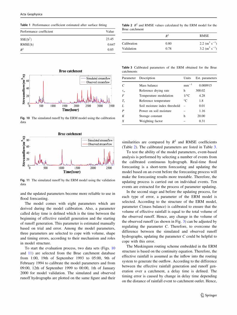
and the updated parameters become more reliable to use in
flood forecasting.
The model comes with eight parameters which are
derived during the model calibration. Also, a parameter
called delay time is defined which is the time between the
beginning of effective rainfall generation and the starting
of runoff generation. This parameter is estimated manually
based on trial and error. Among the model parameters,
three parameters are selected to cope with volume, shape
and timing errors, according to their mechanism and roles
in model structure.
To start the evaluation process, two data sets (Figs. 10
and 11) are selected from the Brue catchment database
from 1:00, 19th of September 1993 to 05:00, 9th of
February 1994 to calibrate the model parameters and from
09:00, 12th of September 1999 to 00:00, 1th of January
2000 for model validation. The simulated and observed
runoff hydrographs are plotted on the same figure and their
similarities are compared by R2 and RMSE coefficients
(Table 2). The calibrated parameters are listed in Table 3.
To test the ability of the model parameters, event-based
analysis is performed by selecting a number of events from
the calibrated continuous hydrograph. Real-time flood
forecasting is a short-term forecasting and updating the
model based on an event before the forecasting process will
make the forecasting results more trustable. Therefore, the
updating process is carried out on individual events. Ten
events are extracted for the process of parameter updating.
In the second stage and before the updating process, for
each type of error, a parameter of the ERM model is
selected. According to the structure of the ERM model,
parameter C(mass balance) is calibrated to ensure that the
volume of effective rainfall is equal to the total volume of
the observed runoff. Hence, any change in the volume of
the observed runoff (as shown in Fig. 3) can be adjusted by
regulating the parameter C. Therefore, to overcome the
difference between the simulated and observed runoff
hydrographs, updating the parameter C could be helpful to
cope with this error.
The Muskingum routing scheme embedded in the ERM
structure is based on the continuity equation. Therefore, the
effective rainfall is assumed as the inflow into the routing
system to generate the outflow. According to the difference
between the effective rainfall generation and runoff gen-
eration over a catchment, a delay time is defined. The
timing error is caused by change in delay time depending
on the distance of rainfall event to catchment outlet. Hence,
Fig. 10 The simulated runoff by the ERM model using the calibration
data
Fig. 11 The simulated runoff by the ERM model using the validation
data
Table 2 R2 and RMSE values calculated by the ERM model for the
Brue catchment
R2 RMSE
Calibration 0.80 2.2 (m3 s-1)
Validation 0.78 3.2 (m3 s-1)
Table 3 Calibrated parameters of the ERM obtained for the Brue
catchments
Parameter Description Units Est. parameters
C Mass balance mm-1 0.000915
sw Reference drying rate h 300.02
F Temperature modulation 1/�C 4.28
Tr Reference temperature �C 1.8
L Soil moisture index threshold – 0.01
P Power on soil moisture – 1.16
K Storage constant h 20.00
X Weighting factor – 0.31
Table 1 Performance coefficient estimated after surface fitting
Performance coefficient Value
SSEðh2Þ 23.45
RMSEðhÞ 0.647
R2 0.85
Acta Geophysica
123

by changing the delay time between the inflow to the
catchment (effective rainfall) and catchment response
(simulated runoff) in the catchment outlet, the difficulties
caused by the timing error (as shown in Fig. 4) could be
solved.
The shape error causes the most troubles in the updating
process. The parameter K is selected due to its mechanism
in the Muskingum routing model. In the experimental
studies, the parameter K is defined as the travel time
through a reach of the river, hence the parameter is linked
with the catchment concentration time and time to peak.
After the relevant parameters selected in the updating
process, the simulated runoff hydrograph for the case
events are updated by changing these parameters. Fig-
ures 12, 13, 14, 15, 16, 17, 18, 19, 20 and 21 show the
observed, simulated and updated hydrograph for each
event.
According to the plotted hydrographs, in some cases,
one error type is highlighted. For example Fig. 13 shows a
significant timing error between the observed and simu-
lated hydrograph and also some error in runoff volume. To
overcome the modelling errors, updating delay time and
parameter C could make the simulated hydrograph closer
to the observed hydrograph. In another evaluation
(Fig. 18), a huge difference in runoff volume is solved by
changing parameter C. In some hydrographs, three types of
errors are observed. In those cases, all of the relevant
parameters are updated at the same time to cope with all
the error types (Fig. 17). Table 4 shows the updated
parameters for the selected events. Also, the R2 and RMSE
coefficients are listed in Table 5. The updated parameters
and performance coefficients confirm how much the model
parameters are capable of improving the simulated hydro-
graph without changing the rest of the model parameters.
Fig. 12 The single event updating from 29/09/93, 23:00 to 02/10/93,
17:00
Fig. 16 The single event updating from 11/10/93, 14:00 to 12/10/93,
21:00
Fig. 13 The single event updating from 29/09/93, 23:00 to 02/10/93,
17:00
Fig. 14 The single event updating from 06/10/93, 06:00 to 08/10/93,
01:00
Fig. 15 The single event updating from 09/10/93, 04:00 to 10/10/93,
03:00
Acta Geophysica
123

A comparison between the hydrographs and the per-
formance coefficients proves that by just updating three
model parameters, significant improvements could be
achieved. This is important in real-time flood forecasting,
because it is easier to adjust 1–3 parameters instead of all 9
model parameters. This process helps to classify the flood
events by providing a lookup table based on the flood
characteristics. In this method, the best parameters are
estimated for each flood event and a number of events are
analysed to provide a lookup table which is based on a
catchment condition. In terms of real-time flood forecast-
ing, after recognising the flood characteristics and weather
condition, the best parameter set could be selected from the
lookup table for forecasting the shape of the hydrograph.
Forecasting the flood hydrograph helps to provide an
overview about the events ahead and provides interesting
information for hydrologists.
Fig. 18 The single event updating from 14/12/93, 23:00 to 16/12/93,
13:00
Fig. 19 The single event updating from 13/11/93, 02:00 to 15/11/93,
02:00
Fig. 20 The single event updating from 14/12/93, 23:00 to 16/12/93,
13:00
Fig. 21 The single event updating from 08/12/93, 06:00 to 09/12/93,
13:00
Table 4 Updated parameters for the selected events
Event ID C K Delay time (h)
1 0.00037378 16.2 6
2 0.00078587 21.3 6
3 0.00098287 13.4 6
4 0.00079987 19.1 5
5 0.000635587 17.5 6
6 0.00130187 9.5 6
7 0.00040587 26.2 8
8 0.00101587 17.4 6
9 0.000986587 29.4 8
10 0.0011321 21.8 5
Fig. 17 The single event updating from 12/10/93, 22:00 to 17/10/93,
00:00
Acta Geophysica
123

Conclusion
The current paper discusses the prevalent errors on runoff
simulation. Occurrence of errors during a simulation pro-
cess is a considerable concern and hence, the model should
be monitored continuously to identify the sources of errors
and make efforts to update the model. The problem is
highlighted in real-time flood forecasting due to limited
time to do the process of model updating. Parameter
updating is one of the existing methods to adjust the model
before starting the forecasting process. In this study, the
ability of the ERM model is investigated to cope with
volume, timing and shape errors. In the first part of the
study, the probable hydrological changes for the model are
illustrated by altering the observed hydrograph. Therefore,
by changing the observed hydrograph, the model parame-
ters should be updated to cope with the newly altered
hydrographs. Due to the importance of time in process of
real-time forecasting and updating, for each error type, one
of the ERM model parameter is assigned to cope with a
certain error type. By selecting the parameters, their abil-
ities are evaluated on real events. Ten runoff events are
selected from a continuous runoff simulation to use in
updating process. The selected events are not simulated
properly in the progress of continuous simulation. In some
cases, the existing one error type (e.g., timing error) is
observed and in some cases the existence of all the error
types are identified, hence updating all the selected
parameters to cope with the errors are required. After
implementing the parameter updating on the selected event
and calculating the performance coefficients, it is con-
firmed that the ERM parameters have reliable flexibility to
cope with the three possible errors in the simulated
hydrographs, without a need to recalibrate the model
parameters.
Consequently, the ERM model parameters are updated
in two ways: (1) updating the model parameters before
starting the forecasting process to reduce difference
between the simulated and observed runoff hydrographs;
(2) predicting the hydrological changes and alerting the
observed hydrograph accordingly, and updating the model
parameters based on the new observed hydrograph. Obvi-
ously, using the updated parameters is more suitable in new
conditions, in comparison with the optimum parameter set.
As for the future work, developing a comprehensive model
to predict the hydrological changes could be mentioned as
a supplementary action to apply in terms of parameter
updating. In this way, the amounts of changes are predicted
and will be applied to the observed hydrograph and the
model will be prepared under new conditions.
References
Arnell NW (1999) The effect of climate change on hydrological
regimes in Europe: a continental perspective. Glob Environ
Change 9(1):5–23
Bartholmes J, Todini E (2005) Coupling meteorological and hydro-
logical models for flood forecasting. Hydrol Earth Syst Sci
Discuss 9(4):333–346
Baymani-Nezhad M, Han D (2013) Hydrological modeling using
effective rainfall routed by the Muskingum method (ERM).
J Hydroinform 15(4):1437–1455
Beven K (1993) Prophecy, reality and uncertainty in distributed
hydrological modeling. Adv Water Resour 16:41–51
Brath A, Montanari A, Toth E (2002) Neural networks and
nonparametric methods for improving real-time flood forecasting
through conceptual hydrological models. Hydrol Earth Syst Sci
Discuss 6(4):627–639
Charlton R, Fealy R, Moore S, Sweeney J, Murphy C (2006)
Assessing the impact of climate change on water supply and
flood hazard in Ireland using statistical downscaling and
hydrological modelling techniques. Clim Change 74(4):475–491
Chiew F, Whetton P, McMahon T, Pittock A (1995) Simulation of the
impacts of climate change on runoff and soil moisture in
Australian catchments. J Hydrol 167(1):121–147
Dibike YB, Coulibaly P (2005) Hydrologic impact of climate change
in the Saguenay watershed: comparison of downscaling methods
and hydrologic models. J Hydrol 307(1):145–163
Table 5 R2 and RMSE values calculated by ERM model for the selected single events
Event Start date End date R2ðsimÞ RMSEðsimÞðm3s�1Þ R2ðupdÞ RMSE ðupdÞðm3s�1Þ
1 29/09/93—23:00 02/10/93—17:00 - 1.190 1.509 0.854 0.389
2 04/10/93—21:00 05/10/93—21:00 0.144 2.636 0.987 0.320
3 06/10/93—06:00 08/10/93—01:00 0.736 2.580 0.853 1.924
4 09/10/93—04:00 10/10/93—03:00 0.134 1.689 0.944 0.427
5 11/10/93—14:00 12/10/93—21:00 - 1.395 3.135 0.563 1.337
6 12/10/93—22:00 17/10/93—00:00 0.828 7.515 0.926 4.917
7 09/11/93—20:00 11/11/93—13:00 - 16.224 2.434 0.763 0.285
8 13/11/93—02:00 15/11/93—02:00 0.605 1.698 0.878 0.941
9 08/12/93—06:00 09/12/93—13:00 - 3.276 1.344 0.825 0.271
10 14/12/93—19:00 16/12/93—13:00 0.359 2.248 0.800 1.255
Acta Geophysica
123

Fang X, Thompson DB, Cleveland TG, Pradhan P, Malla R (2008)
Time of concentration estimated using watershed parameters
determined by automated and manual methods. J Irrig Drain Eng
134(2):202–211
Fu B, Wang J, Chen L, Qiu Y (2003) The effects of land use on soil
moisture variation in the Danangou catchment of the Loess
Plateau, China. Catena 54(1):197–213
Hagg W, Braun L, Kuhn M, Nesgaard T (2007) Modelling of
hydrological response to climate change in glacierized Central
Asian catchments. J Hydrol 332(1):40–53
Haktanir T, Sezen N (1990) Suitability of two-parameter gamma and
three-parameter beta distributions as synthetic unit hydrographs
in Anatolia. Hydrol Sci J 35(2):167–184
Han D (2011) Flood risk assessment and management. Bentham
Science Publishers
Izzard CF, Hicks W (1946) Hydraulics of runoff from developed
surfaces. Highway Res Board Proc 26:129–150
Johnstone D, Cross WP (1949) Elements of applied hydrology.
Ronald Press Company, New York
Kirpich Z (1940) Time of concentration of small agricultural
watersheds. Civ Eng 10(6):362
Lardet P, Obled C (1994) Real-time flood forecasting using a
stochastic rainfall generator. J Hydrol 162(3):391–408
McCalla GR, Blackburn WH, Merrill LB (1984) ‘‘Effects of live
stock grazing on infiltration rates’’. Edwards Plateau of Texas.
J Range Manag 37:265–269
McCuen RH, Spiess JM (1995) Assessment of kinematic wave time
of concentration. J Hydraul Eng 121(3):256–266
Morgali J, Linsley RK (1965) Computer analysis of overland flow.
J Hydraul Div 91(3):81–100
Nguyen M, Sheath G, Smith C, Cooper A (1998) Impact of cattle
treading on hill land: 2. Soil physical properties and contaminant
runoff. N Z J Agric Res 41(2):279–290
Penning-Rowsell EC, Tunstall SM, Tapsell S, Parker DJ (2000) The
benefits of flood warnings: real but elusive, and politically
significant. Water Environ J 14(1):7–14
USDA SCS (US Department of Agricluture Soil Conservation
Service) (1986) Urban hydrology for small watersheds, 2nd
edn. Technical Release 55
Wilby R, Greenfield B, Glenny C (1994) A coupled synoptichydro-
logical model for climate change impact assessment. J Hydrol
153(1):265–290
Wong TS, Chen C-N (1997) Time of concentration formula for sheet
flow of varying flow regime. J Hydrol Eng 2(3):136–139
Xu C-Y (1999) Climate change and hydrologic models: a review of
existing gaps and recent research developments. Water Resour
Manag 13(5):369–382
Yakowitz S (1985) Markov flow models and the flood warning
problem. Water Resour Res 21(1):81–88
Yang X, Michel C (2000) Flood forecasting with a watershed model:
a new method of parameter updating. Hydrol Sci J
45(4):537–546
Younis J, Anquetin S, Thielen J (2008) The benefit of high resolution
operational weather forecasts for flash flood warning. Hydrol
Earth Syst Sci Discuss Discuss 5(1):345–377
Yu P-S, Chen S-T (2005) Updating real-time flood forecasting using a
fuzzy rule-based model/mise a Jour de Prevision de Crue en
Temps Reel Grace a un Modele a Base de Regles Floues. Hydrol
Sci J 50(2):265–278
Acta Geophysica
123