APPLIED NUMERICAL

ELSEVIER MATHEMATICS

Applied Numerical Mathematics 15 (1994) 465-480

Error analysis of numerical schemes for the wave equation in heterogeneous media

Alain Sei *, W.W. Symes

Department of Computational and Applied Mathematics, Rice University, P.0 Box 1892, Houston, TX 77251-1892, USA

Abstract

A family of finite difference schemes for the acoustic wave equation in heterogeneous media is introduced. The precision and computational cost are analyzed in two cases. First, a two-layered medium is considered. The order of convergence at the interface is derived for each scheme. Given an a priori accuracy on the solution, the computational cost is studied *as a function of the order of accuracy of the finite difference scheme. It is demonstrated that this function has a minimum. The previous results are extended to the case of random media by a numerical study. Similar conclusions about precision and cost are found.

Keywords: Wave equation; Heterogeneous media; Numerical schemes; Computational cost

1. Introduction

Finite difference schemes for the wave equation have been extensively studied in homoge- neous media (cf. [12]). The error introduced by the numerical procedure is called dispersion (cf. [ll]). This phenomenon causes different Fourier components of a signal to travel at different speeds and results in a smeared signal.

In heterogeneous media, the effect of the numerical schemes on the reflection and transmis- sion of waves has to be considered. Many authors have studied these properties. Cohen and Joly [2] introduced a compact fourth-order scheme and studied the order of convergence of the reflection coefficient in a two-layered medium. Their results demonstrated a discrepancy between the order of convergence of the reflection coefficient, and the order of convergence of the scheme in homogeneous medium. Brown [l] also conducted an analysis of a two-layered medium and showed that the choice of the interface location in the mesh could increase the order of convergence.

* Corresponding author. E-mail: sei@rice.edu.

0168.9274/94/$07.00 0 1994 Elsevier Science B.V. All rights reserved SSDZ 0168-9274(94)00036-G

466 A. Sei, K W. Symes /Applied Numerical Mathematics 15 (1994) 465-480

However, the study of two-layered media is not enough. There has been growing interest in wave propagation in very heterogeneous media and its implications on seismology theory and models. Frankel and Clayton [4] established the feasibility of finite difference simulations of wave propagation in random media. They then used the simulations as a tool to study the scattering of short period seismic waves by heterogeneities in the Earth’s crust [5]. This scattering affects the waveform, travel time, and the amplitude of waves. Jannaud et al. [6,7] dealt with the attenuation and the anisotropy of seismic waves in random media using computer simulations. In both cases the specific numerical scheme used has been tested for convergence. However, a better understanding and more analysis of finite difference schemes in very heterogeneous media is necessary if we want to use these techniques trustfully. Our goal in this work is to investigate the precision of high-order schemes in heterogeneous media and their computational cost in order to apply finite difference schemes to real (3D) media. The question we want to address is, “What scheme has the lowest cost for a given accuracy on the solution?” We will address that question in the context of a family of numerical schemes based on the first-order system associated with the second-order hyperbolic wave equation. The schemes are indexed by their order of accuracy in space and are second-order accurate in time. First we analyze the two-layered case and then we tackle random media.

The paper is organized as follows. In Section 2 we analyze the truncation error of the second-order scheme at the interface of a two-layered medium. Section 3 shows numerically that the conclusions of Section 2 are still valid for high-order schemes in which the computation of the truncation error is tedious. Section 4 focuses on the computational cost of the different schemes. Given an a priori precision on the solution, the cheapest scheme in terms of floating point operations is found. Section 5 deals with random media as we study numerically the order of convergence. We state our conclusions in Section 6.

2. Analysis of the truncation error

We consider the following model problem. We look for the continuous function u solution of the radiation problem:

a2u a --- at2 ax

=o, XER,

with the following initial conditions:

(1)

where u0 and u1 are smooth functions with support in [w-. The function a is piecewise constant and has a discontinuity in 0. It is defined by

a(x) = i

p x < 0,

3 x > 0. (3)

A. Sei, W. W. Symes /Applied Numerical Mathematics 15 (1994) 465-480 467

We set

u+(x, t) =ll(x, t), x > 0, t > 0,

u-(x, t) =u(x, t), x <o, t >o.

By continuity of u have at the interface x = 0:

u+(o+, t) = up(O-, t), t >, 0. (4)

Using the variational formulation of the problem, it is easy to see that the stress is continuous at the interface x = 0:

au+ al.- a+---- ax (O+, t) = a- -g--(0-, t), t 2 0. (5)

By definition of a we have:

a2u+ a2u+

at2 -a+ ~ =o,

ax2 x > 0, t>o,

a2u-

at2

a_ a2u- ~ =o,

ax2 x < 0, t>o.

Taking the derivative of (4) with respect to time we get

a2u + a2u - at’(O+’ t) = T&O-, t), t 2 0,

and using (6)

a- a2uP ~(0~, t) = a+$$(O+, t), t > 0.

Taking the derivative of (5) with respect to time yields

a-$%(0-, t)=a+-$g(O+, t), t>O,

and using (6) again we have:

(a-1 '$(O-, t) = (a+)2$(O+, t), t 20.

We summarize the preceding result in the following lemma.

Lemma 1. The solution u of the radiation problem (l)-(2) verifies

u+(o+, t) = u-(0-, t),

(6)

(7)

(8) au+ au-

a+- ax (O+, t) = a- -j--(0-, t),

468 A. Sei, W. W Symes /Applied Numerical Mathematics 15 (1994) 465-480

a2u+ a2u- a+- ax2 (O+, t> = a- g(O-, t>,

(a+)2$ (O+, t) = (a-)‘$(O-, t).

(9)

(10)

We now consider a family of numerical schemes based on finite difference approximations of the first derivative. Those schemes can be written as approximations of the first-order system associated with the second-order hyperbolic wave equation. We introduce two different grids corresponding to the following functional spaces:

G = 4 E L2P) $J = E

i I ~il[(i-1,2)h,(i+l,2)h, x

i= -_m ( 4 )

L2* = 4 EL2W 4 = YE ~i+l,2l~iax,(i+I)~x,(X) 1 I

* i= -_m I

Now we define the finite difference operator A, by:

AL:L;+L2.+,

u HAL,%+ l/2 = Ih ~rui+,-%,+J. 1=1

The coefficients (/31)1=1 ,,, L are chosen so that A, is an approximation of order 2L of the first derivative at the point 5 +’ i. The fully discrete (2-2L) scheme for Eq. (1) is:

.;+I - 2%; +u,“-l

At2 +fAL(ai+~/*ALU~+1/2 ) =o. (11)

This scheme can be written as a first-order system using:

“r+1/2 - .y+l -q

- 1 At ’ w:+1,2 =ALUF+l,*;

we can write (11) as follows (see Appendix A):

uy+lP I

- up-v 1

At = -fAL(ai+l/2w~+l/2)~

e++l1/2 - Y?+ l/2

At = ALun+ 1’2)i+ 1,2. (

This is the discrete equivalent of the first-order hyperbolic system:

au a - = --(a. w), at

aw au _=_ at ax’

(12)

A. Sei, W. W. Symes /Applied Numerical Mathematics 15 (1994) 465-480 469

Luo and Schuster [8] proposed this scheme (12) with a second-order approximation in space. The family of schemes introduced is the extension of their scheme to an arbitrary order in space. These schemes are not equivalent to the compact schemes introduced by Dablain [3] for homogeneous media and by Cohen and Joly [2] for heterogeneous media.

The discontinuity in the medium arises only in the spatial derivative. Therefore to analyze the truncation error at the interface it is relevant to consider the semi discrete equation given by:

d2ui - +fAL(ai+I/*ALUi+I/2 dt2

) =o.

With L = 1 (second-order approximation in space) we have:

d$ _ ;(ai+I,2( “i+;-“) _&r,,( “i-,“i-1)) =O.

At the interface x = 0 we have:

~-~(~l/*(~)-a_l/z(u~~u-~))=o,

which because of the definition of a is

(13)

The solution u is equal to the sum of the incident wave ui and the reflected wave u, on one side of the interface, and is equal to the transmitted wave u, on the other side of the interface. Using d’Alembert’s formula, if u. and ur are Cm(R) then ui, u, and u, are Cm(R) in space. Therefore u is C” on (-co; 0) U (0; +m). Assuming u. and u1 are C”(R) then u+ and u- are smooth functions and we can write:

u1- uo ~ = (L&j+>’ + ;&gr + $u;y + O(h3), h

uo -u-1

h = (u,>‘- &Jrt + ;(u~)“‘+ O(h3),

where <u$Y = au ‘(0 *, t)/k. The truncation error in x = 0, Eo(t), measures how closely the discrete equation is an approximation of the continuous equation. We let the exact solution u satisfy the discrete equation and with the previous regularity assumptions compute the leading error term. We have:

&o(t) = S(t) - $(u+(u:r(t) - a-(u;>l(t)) + ;(u+(u;)yt) + u-(u;)“(t))

+ &z+(u:)ryt) -u-(U;)“‘(t)) + O(h2), t>o.

470 A. Sei, W. W. Symes /Applied Numerical Mathematics 15 (1994) 465-480

Using Lemma 1:

af(u,+>l(t) =a-(u;>l(t), t > 0,

af(uo+)“(t) =u-(u;)“(t), t 2 0;

SO

&o(t) = 2(t) -u+(u,t)yt) + ;(u+(u;)yt) -u-(uJ”‘(t)) +O(h2), t > 0.

Using (4) and (6) we have

S(t) -a+(Uof)“(t) = d*u+ $-(t)-a+(u;)“(t)=o, t>o;

therefore the truncation error is given by:

q)(t) = ;(u+(u;)yt) -u-(uJ”‘(t)) + O(h2), t 2 0. (14)

The presence of the discontinuity reduces the accuracy of the scheme at the interface. We have proved the following proposition:

Proposition 2. The convergence of the scheme (13) at a point of discontinuity of the coefficient a is linear with the space step h.

This result is similar to those obtained in [l] by Laplace transform or in [lo] when no special treatment is applied to the interface.

3. Study in two-layered media

We now turn to the analysis of the accuracy of higher-order schemes for the acoustic wave equation in heterogeneous media. The medium is characterized by its density p(x) and its velocity c(x). The acoustic wave equation relates the source located in x = s with waveform f to the pressure u according to:

--- (15)

The heterogeneous acoustic wave equation (1.5) is approximated by the following finite difference scheme:

q+‘-_2.q+q’ 1

pi. cfAt* +*A,

Pi + l/2 ALx+1,2 = %f n* (16)

To analyze the effect of a discontinuity for higher-order schemes we proceed numerically. We define a two-layered medium and compute the seismogram S at the source as a function of time. The source is located on the left-hand side of the interface. After the first arrival we

A. Sei, W. W Symes /Applied Numerical Mathemaiics 15 (1994) 465-480 471

1 .o

0.5

a, z z

0.0

L

-0.5

-1 .o

‘:,I’ L

~ I---

0.10 i-i-- ,-- __L

0.20 0.30

Time

Fig. 1. The direct and reflected waves.

record the reflected wave bouncing off of the interface. Since we are interested in the properties of the scheme at the interface we want to study the reflected part of the signal. This part is easy to isolate because we choose a Ricker source which is for practical purposes compactly supported in time. Furthermore the reflected wave will have an amplitude less than the direct wave since the reflection coefficient is less or equal to one (see Fig. 1). We chose the following medium for the study.

0.40

P(X) = :‘T5 i x < 0,

t . , x > 0, :(

.l The reflection coefficient is equa in closed form. Then once we normalized L2 error defined by

N

Ix) = i

1500, x-co, 2000, x > 0.

to 0.4. In a two-layered medium we know the exact solution have the numerical and exact solutions, we compute the

c I S,,,(At, h; n) - S,,(n . At) I 2At E(L, At, h) = ‘=’ N

c S,2,(nAt)At (17)

,I = 1

with S,,,(At, h; YE . At) = uJ”, S,,(t) = u(s, t> and T,,, is the recording time. The order of convergence of the numerical solution is given by plotting the function

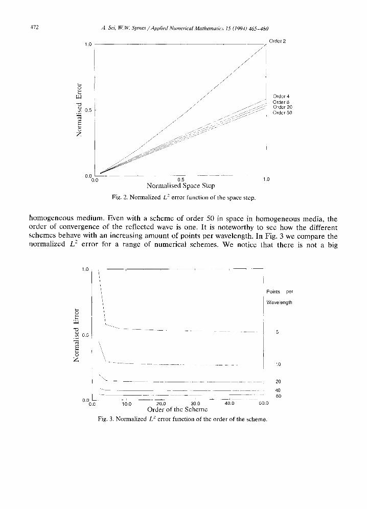
h - E( L, At, h) for fixed L and At. The resulting curves are displayed in Fig. 2. They confirm the statement of Proposition 2. The convergence for the high-order scheme is linear with the space step h. Furthermore it is independent of the order of the numerical scheme in

472 A. Sei, W W. Symes /Applied Numerical Mathematics 15 (1994) 465-480

1 .o Order 2

0.5

Normalised Space Step

Fig. 2. Normalized L* error function of the space step.

homogeneous medium. Even with a scheme of order 50 in space in homogeneous media, the order of convergence of the reflected wave is one. It is noteworthy to see how the different schemes behave with an increasing amount of points per wavelength. In Fig. 3 we compare the normalized L2 error for a range of numerical schemes. We notice that there is not a big

Points per

Wavelength

_.___I_ 2 ~,___ L-- --__ -< ~~

10.0 20.0 30.0 40.0 c

Order of the Scheme t0.C

5

10

20

40 80

)

Fig. 3. Normalized L2 error function of the order of the scheme.

A. Sei, W.W Symes /Applied Numerical Mathematics 15 (1994) 465-480 473

-- Numerical Solution

- Exact Solution

G z 0.0

‘\ c;: \ \

-0.1 j \ \ -I \

-0.2 \ \ \ \

-0.3 \ MInImum Period

Fig. 4. The shift between the exact and numerical solution for a relative L2 error of 10%.

difference between the (2-4) scheme and higher-order schemes as soon as we control disper- sion effects, that is after 10 points per wavelength. This conclusion is similar to the one for homogeneous media which suggests that dispersion is still a major contribution to the error [9].

4. Cost analysis for a two-layered medium

We now look for the cheapest scheme in terms of number of operations which fulfills a certain error percentage on the solution. We chose 10 percent of error on the L’ relative error. This corresponds to a shift between the numerical and exact solution of one-eighth of a period (cf. Fig. 4). To find the optimal numerical parameters we proceed by a simple search through the possible values of the two non-dimensional parameters Iv,, the number of points per minimum period, and NA, the number of points per minimum wavelength. The Ricker source is in practice band-limited. It is characterized by a central frequency F,, and the cutoff frequency is defined by F,,, = 2.5F,,. Therefore the minimum period is Tmin = l/F,,,, and the minimum wavelength is Ami, = cmin . Tmin. Thus the number of points per minimum period 1yT and the number of points per minimum wavelength Iv, are given by

AI7li” NA = -

Tmin

h ’ NT=-

At ’

The computational cost associated with the different schemes is taken here as the total number of floating point operations. It is defined by

Cost = NL x N,; x N, ,

474 A. Sei, W. W. Symes /Applied Numerical Mathematics 15 (1994) 465-480

1 .o

/

o,oo,o_.~_~.-.- 10.0 20.0 30.0 AL _L 40.0 ~~ i---- 50.0

Order of the Scheme

Fig. 5. The normalized cost for an error of 10% in 1D.

where NL is the number of operations per point and time step for the scheme of order 2L in space, N, is the number of points in one direction (the domain is a square or a cube), N, is the number of time steps and y1 (= 1, 2, 3) the dimension of the domain.

Nyquist criterion imposes that NA > 2 and the stability criterion imposes that

c,,, . At ‘rnin Nh h

<a(L) - NT>-- cmax 49

= NFi”.

This way the choices of NT and NA satisfy the stability condition. For a fixed N,, we compute the error for NT = NFi” to NT = NFaX. We fixed NFax to 300.

We can extend our results to 2D or 3D problems by assuming that the interface is aligned with the grid and parallel to the axis x = 0 in 2D or the plane x = 0, y = 0 in 3D. Then sending a plane wave modulated by the shape of the Ricker gives the preceding 1D problem.

The first couple (N,, N,) fulfilling the precision criterion gives the least cost for the scheme considered because the cost is proportional to Nr . NT. Our results are summarized in Figs. 5 and 6 for the different dimensions. The important feature to notice is that in 2D and 3D the cost has a minimum for the fourth-order scheme. This same observation was done in the analysis of dispersion error in homogeneous media [9]. The difference between 1D and 2D or 3D comes from the expression of the cost. In 1D the cost is linear in all of its variables NL, NT and N,. In 2D or 3D the cost becomes quadratic or cubic in Nh. Therefore the improvement in the number of points per wavelength for the fourth-order scheme versus the second-order scheme is not offset by the increase in the number of operations per node like in the 1D case.

The linearity of the cost after the minimum comes from the linearity of the number of operations with the order of the scheme. The other parameters NT and NA change very little because all the schemes have the same order of convergence at the interface.

A. Sei, W. W. Symes /Applied Numerical Mathematics 15 (1994) 465-480 475

0.0 in 1

0.0 10.0 40.0 I _~~~~~_20~o~,_'~30.0~~~~ 50.0

Order of the Scheme Fig. 6. The normalized cost for an error of 10% in 2D and 3D.

5. Study in random media

The application of finite difference schemes to very heterogeneous media poses many questions. What is the order of convergence in such media? Does a finite difference scheme minimize the computational cost?

We choose to study random media characterized by a Gaussian correlation function. To construct a Gaussian velocity distribution, one must choose an average velocity and a standard deviation from that average [5].

We consider an average velocity of 1500 m/s, an average density of 1 kg/m and a standard deviation of 10%. To avoid problems with the source, we embed the random medium in a homogeneous matrix with the same average values. The resulting density and velocity are displayed in Fig. 7. An incoming wave from the left-hand side is sent into this heterogeneous zone. Reflections from the boundary are avoided by creating a large homogeneous matrix.

Practically, the random medium is generated on a grid with a given spacing hmedium. If the space step h in the numerical scheme is not an integer multiple of hmedium we locate incorrectly the different interfaces of the medium. We are interested in the order of convergence and want to avoid interpolation error. So, we specify a certain number of points per medium spacing so that precisely hmedium/h is an integer. This way the random medium looks like a succession of more or less finely sampled random valued layers. It is a generalization of the two-layered medium. In the example chosen we have the following characteristic values:

c,,,~,, = 1127.54 m/s, cmax = 1850.13 m/s,

pmin = 0.756 kg/m, p,, = 1.237 kg/m,

hmin = 15.03 m, F,,, = 75 Hz.

The medium spacing is hmedium = 5 m.

476 A. Sei, W W Symes /Applied Numerical Mathematics 15 (1994) 465-480

2000.0

(4

’ ooo&oo.o

1.3

1.1

E- ??I Y S. ,% s 0

0.9

0.7 L 2000.0

lb)

2500.0 3000.0 3500.0

Distance (m)

h / -‘:I’ 1

2500.0 3000.0 3500.0 Distance (m)

Fig. 7. The density and velocity distributions.

40&o

In such heterogeneous media an analytical result like Proposition 2 is possible only locally. To know the global order of convergence we proceed numerically. A big difference with the previous case of two-layered medium is that the exact solution is not known. So we computed

A. Sei. W. W. Symes /Applied Numerical Mathematics 15 (1994) 465-480 417

1 .o 2.0

Time

Fig. 8. The reference solution.

two numerical solutions using two different schemes (the fourth-order and the sixth-order) and very small space and time steps. We chose 50 points per wavelength and 400 points per period. We obtained a normalized L2 error between the “two” solutions of 1.8 * 10-j. In the L’ sense

// /

/ /I/

i

/

_’

,A ,/’

,’

/ ,’ ___,,” ’

iI’ 3rder 2

Order 4 Order 6 Order 8 Order 20

1 "."O.O ^_

03 _ ̂ 1.”

Normalised Space Step Fig. Y. Normalized L’ error function of the space step for the random medium,

478 A. Sei, W W. Symes/Applied Numerical Mathematics 15 (1994) 465-480

this is quite small considering the numerous oscillations of the seismogram, see Fig. 8. The simulation with the fourth-order scheme is chosen as reference. The seismogram is the recording of the pressure field u at the source where a Ricker wavelet was set off at t = 0. The results are summarized in Fig. 9. They show that in highly heterogeneous media the conver- gence is linear. Furthermore we notice that schemes of order higher than four do not improve the accuracy. A parallel can be drawn with the cost analysis of the previous section. Since schemes higher than four do not improve accuracy, the number of points per wavelength necessary for a given accuracy will be the same for all these schemes. But, the computational cost is linear with the order of accuracy of the scheme, so the higher the scheme the higher the cost. Therefore the fourth order scheme will be the cheapest scheme to use in very heteroge- neous media.

6. Conclusions and discussion

In this paper our goal was to investigate the precision of finite difference simulations of seismic waves in highly heterogeneous media keeping in mind the computational cost of the simulations. We introduced a family of numerical schemes based on the first-order system associated with the acoustic wave equation. The truncation error in a two-layered medium has been analyzed. We showed that the truncation error at the interface for the (2-2) scheme is a linear function of the space step. For higher-order schemes a numerical study confirmed that result.

The computational cost of the different schemes has been studied as a function of the order of accuracy of the scheme for a given precision on the solution. It is demonstrated that the computational cost has a minimum for the fourth-order scheme. This result can be explained as follows. First, the number of operations per node grows linearly with the order of the scheme and second, all the schemes have the same order of convergence.

We then considered random media as an example of highly heterogeneous media. In that case the exact solution is not known in closed form. We computed a reference solution with very fine time and space steps. The numerical study showed in that case also that the convergence in such media is linear with the space step and is independent of the order of the scheme in homogeneous media. The accuracy is not improved by schemes higher than the fourth-order scheme. Therefore the computational cost of such schemes is higher than the fourth-order scheme for the same accuracy.

Acknowledgement

The authors thank Jamie Meighen-Sei for helpful remarks and discussions and Lionel Jannaud for providing the random medium code.

A. Sei, W. W. Symes/Applird Numerical Mathematics 15 (1994) 465-480 47’)

Appendix A

In order to write the numerical scheme as a first order, we use the following quantities:

u”+‘/2 = u;+1 -u”

1 At ’ Y&2 =ALG,2’

Using Eq. (11) we can write:

47+1/2 - 44/2

At = -%(%+,,2wL,2).

We have now to see what first-order equation w satisfies. We can write

n+l Wi+ l/2 - Y?+ l/2

At = &4LG,2 -API’+,,:)

Finally, we can write the second-order scheme

I

un+ l/2 - U”- l/2

At = -tAL(ai+~/*W~+1/2)~

(11) as the following first-order system:

W?+’ r+1/2-c+1,2

At =A L’r+1/2

L r+1/2

References

[l] D. Brown, A note on the numerical solution of wave equation with piecewise smooth coefficients, Math. Camp. 42 (1984) 369-391.

[2] G. Cohen and P. Joly, Fourth order schemes for the heterogeneous acoustic equation, Comput. Methods Appl. Mech. Engrg. 80 (1990) 397-407.

[3] M.A. Dablain, The application of high-order differencing to the scalar wave equation, Geophysics 51 (1986) 54-66.

[4] A. Frankel and R.W. Clayton, Finite-difference simulation of wave propagation in two-dimensional random media, Bull. Seismol. Sot. Amer. 74 (1984) 2167-2186.

[5] A. Frankel and R.W. Clayton, A finite-difference simulation of seismic scattering: implications for the propagation of short-period seismic waves in the crust and models of crustal heterogeneity, J. Geophys. Research 91 (1986) 646556489.

480 A. Sei, W W. Symes /Applied Numerical Mathematics 15 (1994) 465-480

[6] L. Jannaud, P.M. Adler and C.G. Jacquin, Frequency dependence of the Q factor in random media, J. Geophys. Research 96 (1991) l&233-18,243.

[7] L. Jannaud, P.M. Adler and C.G. Jacquin, Wave propagation in random anisotropic media, J. Geophys. Research 97 (1992) 15,277-15,289.

[8] Y. Luo and G. Schuster, A parsimonious staggered grid differencing scheme, Geophys. Research Lett. 17 (1990). [9] A. Sei, Computational cost of finite-difference elastic waves modeling, in: Proceedings 63rd SEC Annual

Meeting, Washington, DC (1993) 1065-1068. [lo] A.N. Tikhonov and A.A. Samarskii, Homogeneous difference schemes, Zh. Vychisl. Mat i Mat. Fiz 1 (1961)

S-63. [ll] L. Trefethen, Group velocity in finite difference schemes, SIAM Reu. 24 (1982) 113-136. [12] R. Vichnevetsky and J.B. Bowles, Fourier Analysis of Numerical Approximations of Hyperbolic Equations, SIAM

Studies in Applied Mathematics (SIAM, Philadelphia, PA, 1982).