error propagation modeling in gis polygon · pdf fileerror propagation modeling in gis polygon...

ERROR PROPAGATION MODELING IN GIS POLYGON OVERLAY

Jinda Sae-Jung, Xiao Yong Chen, Do Minh Phuong

Department of Remote Sensing and Geographic Information Systems, Asian Institute of Technology, Thailand

KEY WORDS: Error Propagation; Overlay Analysis; Vector Data; GIS; Sliver ABSTRACT: A spatial error may refer to the difference between a measured value and the “true” value or the estimated uncertainty with respect to a given observation or set of observations which is the error contained in the coordinate values of points, lines and volumes. This paper focuses on developing a methodology for error handling and error propagation modeling in spatial database with GIS. The main target of this study is error propagation on vector polygon overlay in a GIS. An error model was developed to examine errors from its component layers. Error simulations on intersection points proved an important fact that overlay error can be calculated from its components. This error is an average of the component errors. Sliver error was also analyzed and simulated to come up with a solution for solving this common error in overlaying polygons. It is recommended to split-and- merge slivers, not to delete nor combine. In most cases, the splitting line can be drawn to follow proportional weights to the errors in two boundary lines from their original polygons.

1. INTRODUCTION

There are several cases of error while a set of data is processed in a GIS. Errors can occur depending on the knowledge of data analysts and the sophistication of instruments. For example, an operator can hardly track precisely the lines to be digitized during a map digitizing task and so on. Positional accuracy is defined by how well the true measurements of an object on the earth’s surface matches the same object stored as a series of digital coordinates in a GIS data layer. As a matter of fact, the positional error propagation is one of the most complicated and unpredictable issues in GIS analysis which will be considered in this paper. As there are many types of errors, this paper provides a method for estimating positional error of geospatial data focusing on polygon vector overlay. It is divided to 3 sections to measure and analyze the error propagation from the original polygons to the processed polygon which are 1) error propagation along the boundary line of overlay polygon, focus on the intersection outputs 2) error of the intersection points of the output polygons which propagate from the same point of original polygons, and 3) slivers and gaps which are general errors occurred after overlay processing. After identify and measurement all of the error propagation, some kind of error such as slivers will be management with the problem with the suitable solution.

2. ERROR MODELING FOR INTERSECTION POINT OF THE OVERLAID BOUNDARY POLYGONS

To foster error examination when overlaying some polygon layers, it is necessary to have a close look into the common points of those layers, which are the intersection points when two boundary lines of two polygons cut each other. The special characteristics of those intersection points, is even though they are derived from various sources of data with different accuracy, they are wearing the same error to their true points. Two polygons intersect to each other at least at two or more points. This intersection creates real overlay product and some additional by products, which are errors. Obviously, error made by polygon intersection is mostly sliver.

First, select the point intersection from the overlaid polygons to generate the error normal distribution. By the theory, at the intersection point, A and B are the same true value and the error of A should equal to B and therefore, the error at the intersection point is the point which the error is in between error from A and B polygon. . Experiments have been made to examine how the error made by the combination of source for A and source for B changes.

825

The International Archives of the Photogrammetry, Remote Sensing and Spatial Information Sciences. Vol. XXXVII. Part B2. Beijing 2008

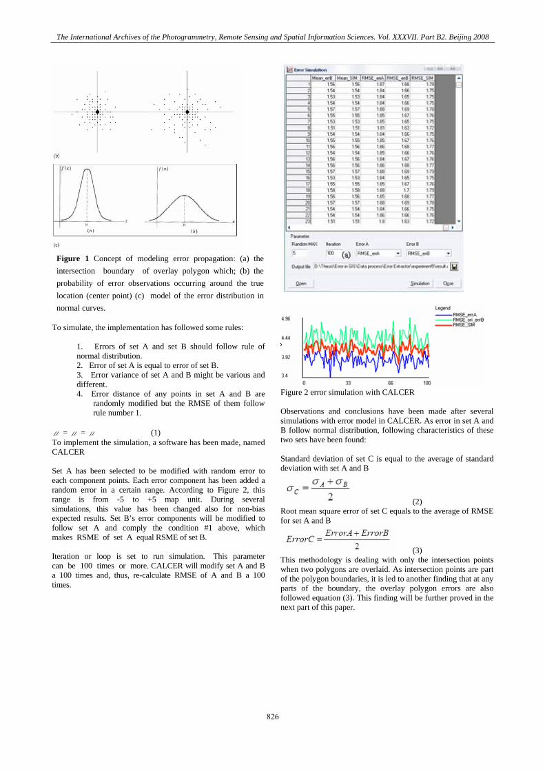
Figure 1 Concept of modeling error propagation: (a) the intersection boundary of overlay polygon which; (b) the probability of error observations occurring around the true location (center point) (c) model of the error distribution in normal curves.

To simulate, the implementation has followed some rules:

1. Errors of set A and set B should follow rule of normal distribution. 2. Error of set A is equal to error of set B. 3. Error variance of set A and B might be various and different. 4. Error distance of any points in set A and B are

randomly modified but the RMSE of them follow rule number 1.

μ = μ = μ (1) To implement the simulation, a software has been made, named CALCER Set A has been selected to be modified with random error to each component points. Each error component has been added a random error in a certain range. According to Figure 2, this range is from -5 to +5 map unit. During several simulations, this value has been changed also for non-bias expected results. Set B’s error components will be modified to follow set A and comply the condition #1 above, which makes RSME of set A equal RSME of set B. Iteration or loop is set to run simulation. This parameter can be 100 times or more. CALCER will modify set A and B a 100 times and, thus, re-calculate RMSE of A and B a 100 times.

Figure 2 error simulation with CALCER Observations and conclusions have been made after several simulations with error model in CALCER. As error in set A and B follow normal distribution, following characteristics of these two sets have been found: Standard deviation of set C is equal to the average of standard deviation with set A and B

(2) Root mean square error of set C equals to the average of RMSE for set A and B

(3) This methodology is dealing with only the intersection points when two polygons are overlaid. As intersection points are part of the polygon boundaries, it is led to another finding that at any parts of the boundary, the overlay polygon errors are also followed equation (3). This finding will be further proved in the next part of this paper.

826


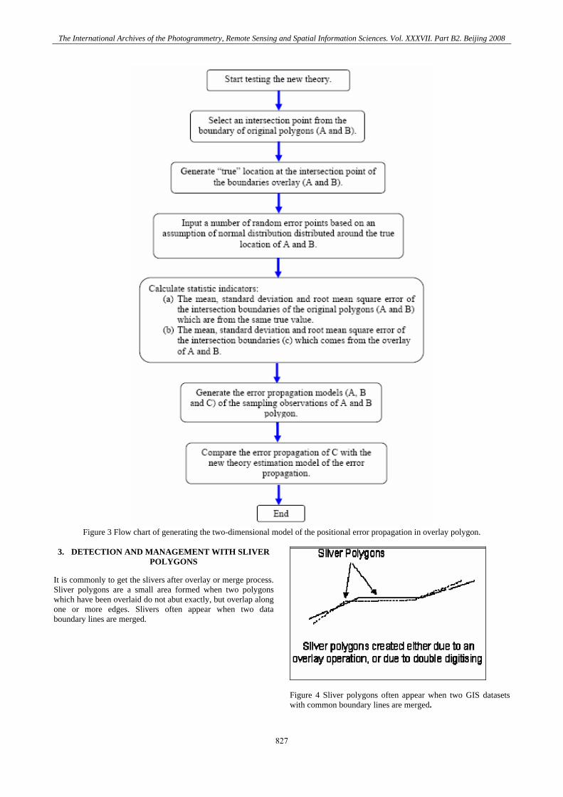
Figure 3 Flow chart of generating the two-dimensional model of the positional error propagation in overlay polygon.

3. DETECTION AND MANAGEMENT WITH SLIVER

POLYGONS

It is commonly to get the slivers after overlay or merge process. Sliver polygons are a small area formed when two polygons which have been overlaid do not abut exactly, but overlap along one or more edges. Slivers often appear when two data boundary lines are merged.

Figure 4 Sliver polygons often appear when two GIS datasets with common boundary lines are merged.

827


To solve these kinds of errors, first we need intelligent criteria to distinguish between slivers and real polygons to detect and solve the problem which is follow: • Area: Slivers are small • Shape: slivers are long and thin • Number of arcs: slivers generally have only 2 bounding arcs while real polygons have only 1 arc. In Figure 3.8 shown an example, if a "red" arc between polygons A and B is overlaid on a "blue" arc between polygons 1 and 2, the slivers will alternate between A2 and B1 • Chaining: slivers tend to occur in chains

Figure 5 Workflow of Measurement of Sliver and gap polygons To identify the sliver polygons, it is important to look at the ratio between a polygon’s perimeter and its area. For P is the perimeter of a polygon

A is the area e is the ratio following this equation:

(4) • Circle polygon

(5) Where R is the radius of the circle. • Square polygon

(6) Where R 1 is the first side of the rectangle.

R 2 is the second side of the rectangle.

For given , then

(7) It is obvious that when k ≠ 1

(8) From case 1,2 and 3, it is pointed out that a sliver polygon is the one which satisfies e > 4. However, this value of e depends on the decision when one is going to eliminate slivers. Experiments with rectangles show that: k=5 e=5.34 k=6 e=5.7 k=7 e=6.0 k=8 e=6.3 . . When k>5, e ≥ 5.3, the rectangle can be eliminated a sliver. For statistic determination, k can be selected from 5, 6 or 7, with corresponding e from 5.3, 5.7 or greater. It is apparent that when a polygon and a rectangle are of the same size (area), the perimeter of the rectangle is the smaller. Therefore, for the case of the polygon, k can be determined ≥ 5 and so e ≥ 5.34.In this study, the polygon which has been selected to be a sliver should have e ≥ 5.3 or e ≅ 5.7 ± 0.5. When a sliver is detected, it can be replaced by an arc along its center line or should be merged with the most suitable of their neighbors. If one of the bounding arcs that make up an area feature is dropped, the feature will merge with whichever of its neighbors the line borders. Thus, if a suitable neighbor can be found for the suspected sliver polygon to merge with, the line separating them simply needs to be removed. In general, when two polygons overlay, it creates two or more intersections and some create slivers also. Sliver is considered error of the overlaying process. To solve the sliver, there is a solution: split sliver should be the best solution because it equally distributes error of the overlay components. To come up with the solution of splitting the sliver, it is clear that the solution should be able to draw a polyline which (i) splits the sliver into two parts; and (ii) equally distributes error of its original component A and B.

828


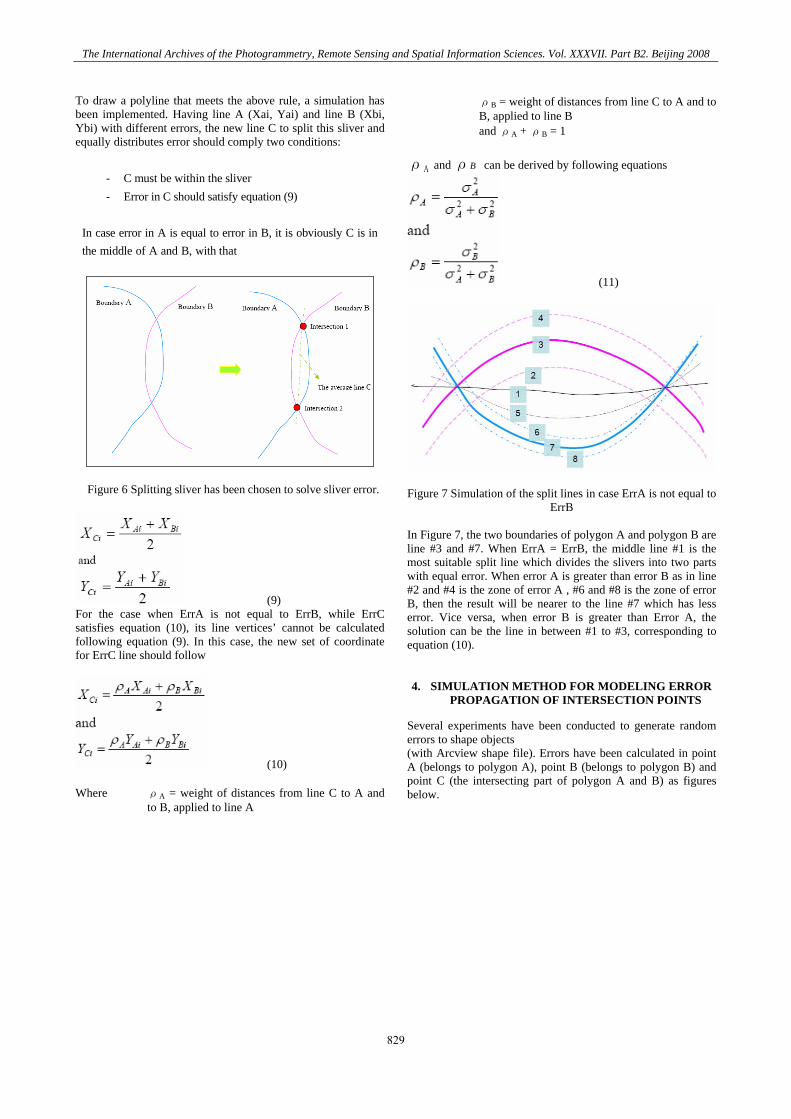
To draw a polyline that meets the above rule, a simulation has been implemented. Having line A (Xai, Yai) and line B (Xbi, Ybi) with different errors, the new line C to split this sliver and equally distributes error should comply two conditions:

ρB = weight of distances from line C to A and to B, applied to line B and ρA + ρB = 1

ρA and ρB can be derived by following equations

- C must be within the sliver

(11)

- Error in C should satisfy equation (9)

In case error in A is equal to error in B, it is obviously C is in the middle of A and B, with that

Figure 6 Splitting sliver has been chosen to solve sliver error. Figure 7 Simulation of the split lines in case ErrA is not equal to ErrB

(9)

In Figure 7, the two boundaries of polygon A and polygon B are line #3 and #7. When ErrA = ErrB, the middle line #1 is the most suitable split line which divides the slivers into two parts with equal error. When error A is greater than error B as in line #2 and #4 is the zone of error A , #6 and #8 is the zone of error B, then the result will be nearer to the line #7 which has less error. Vice versa, when error B is greater than Error A, the solution can be the line in between #1 to #3, corresponding to equation (10).

For the case when ErrA is not equal to ErrB, while ErrC satisfies equation (10), its line vertices’ cannot be calculated following equation (9). In this case, the new set of coordinate for ErrC line should follow

(10)

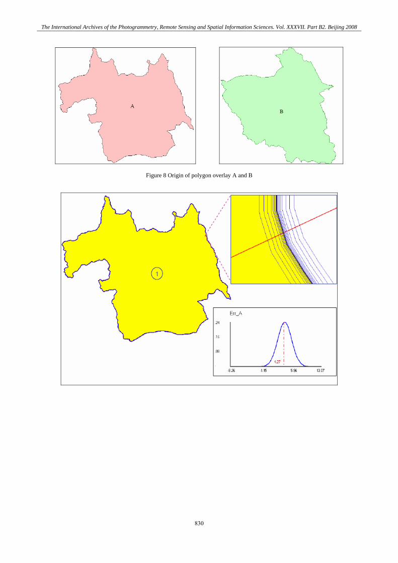
4. SIMULATION METHOD FOR MODELING ERROR PROPAGATION OF INTERSECTION POINTS

Several experiments have been conducted to generate random errors to shape objects (with Arcview shape file). Errors have been calculated in point A (belongs to polygon A), point B (belongs to polygon B) and point C (the intersecting part of polygon A and B) as figures below.

Where ρA = weight of distances from line C to A and

to B, applied to line A

829


Figure 8 Origin of polygon overlay A and B

830


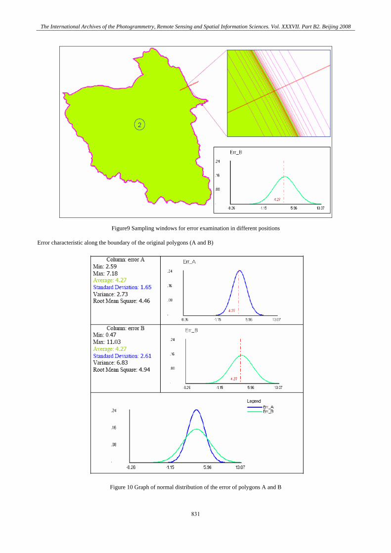
Figure9 Sampling windows for error examination in different positions

Error characteristic along the boundary of the original polygons (A and B)

Figure 10 Graph of normal distribution of the error of polygons A and B

831


Figure 11 Error at the intersection point of A and B Error characteristics at intersection point (C)

832


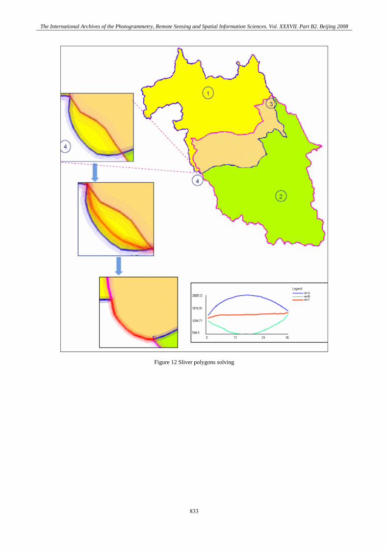
Figure 12 Sliver polygons solving

833


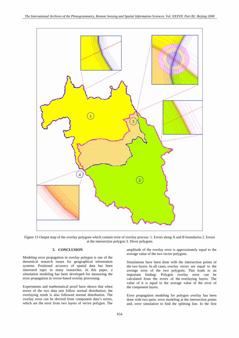
Figure 13 Output map of the overlay polygons which contain error of overlay process: 1. Errors along A and B boundaries 2. Errors

at the intersection polygon 3. Sliver polygons

5. CONCLUSION

Modeling error propagation in overlay polygon is one of the theoretical research issues for geographical information systems. Positional accuracy of spatial data has been interested topic in many researches. In this paper, a simulation modeling has been developed for measuring the error propagation in vector-based overlay processing. Experiments and mathematical proof have shown that when errors of the two data sets follow normal distribution, the overlaying result is also followed normal distribution. The overlay error can be derived from component data’s errors, which are the error from two layers of vector polygon. The

amplitude of the overlay error is approximately equal to the average value of the two vector polygons. Simulations have been done with the intersection points of the two layers. In all cases, overlay errors are equal to the average error of the two polygons. This leads to an important finding: Polygon overlay error can be calculated from the errors of the overlaying layers. The value of it is equal to the average value of the error of the component layers. Error propagation modeling for polygon overlay has been done with two parts: error modeling at the intersection points and, error simulation to find the splitting line. In the first

834


simulation, the number of error points in the first data set (set A) may be equal or not equal to the number of error points in the second data set (set B). As the matter of fact, both two points intersect at the same point and so, bear the same error. The simulation process should ensure that errors added to each set to be random and it maintain the equalization of error in both sets. With support of computer programming, this simulation can be implemented with 100, 1000 or more iterations. This is necessary because it can help avoid bias in sampling selection. In the second simulation, a hypothesis has been made which pointed out that the splitting line error graph is the line locating in the middle of the error lines of the two boundaries. Simulation is based on the repetition of calculating new splitting line and graphing it to find the best matched to the hypothesis error line. Experiments have proved that the line which has error graph matched best to the hypothesis line is exactly following equation (10). This equation is a practical equation which helps calculate and draw the spitting line which solves the sliver cases.

REFERENCES

Ali Abbaspour, R., 2002, Error propagation in overlay analysis in GIS, MSc. Thesis,Surveying and Geomatic Engineering Dept., University of Tehran, Iran. Brunsdon,C., and Openshaw,S., 1993, Simulating the Effects of Error in GIS. In Geographic Information Handling: Research and applications, edited by P.Mather( Chichester: John Wiley & Sons). Goodchild, MF.,1999, Keynote speech: Measurement-based GIS. In Proceedings of The International Symposium on Spatial Data Quality, edited by Shi, W., Goodchild, M.F. and Fisher, P.F. (Hong Kong: Hong Kong Polytechnical University) pp. 1-9. Goodchild,M. and Hunter,G.,1997, A simple positional accuracy measure for liner features. Geographical Information Science,V.11,pp.299-306.

Goodchild ,M.F. and Zhang,J.,2002,Uncertainty in Geographical Information. New York: Taylor&Francis. Heuvelink,G.M.B., and Burrough P.A., 2002,Propagation of Errors in Spatial Modeling with GIS. International Journal of Geographic Information System,Vol.3, No.4. Newcomer,J.A. and Szajgin,J., 1984,Accumulation of thematic map errors in digital overlay analysis. The American Cartographer,11,pp.58-62. Openshaw ,S.,Charlton,M.and Carver,S., 1991, Error propagation: A Monte Carlo simulation. In Handling Geographical Information, edited by I.Masser and M. Blakemore (New York: Longman),pp.78-101. Podobnikar,T.,1998, Positional error modeling using Monte Carlo simulation. Available online : http://www.geogr.muni.cz/lgc/gis98/proceed/PODOBNIK.html Shi,W. and Liu,W.,2000, A stochastic Process-Based Model for positional Error of Line Segments in GIS. International Journal of Geographical Information Science,14,1:51-66. United States Geological Survey (USGS), 2000, National Map Accuracy Standard. Available online:http://rockwebcr.usgs.gov/nmpstds/nas.html Veregin,H., 1995, Developing and Inspection an Error Propagation Model for GIS Overlay. International Journal of Geographical Information Science,14,51-66. Zhang ,J.and Kirby,R.P., 2000, A geostatistical approach to modeling positional errors in vector data. Transactions in GIS,4,pp.145-159. Zhang, J. and Goodchild,M.F.,2002, Uncertainty in Geographical Information. Deriving Mean Lines and Epsilon Error N=Bands from Simulated

Data.pp.218-224.

835


836

error propagation modeling in gis polygon · pdf fileerror propagation modeling in gis polygon...

Documents