escape from the market: discretionary liquidity trading

Escape from the Market: Discretionary Liquidity Trading

Joon Chae*State University of New York at Buffalo, NY USA

Abstract

Using two types of corporate events, a scheduled announcement andan unscheduled announcement, I investigate the effect of informationasymmetry on trading volume. Only before a scheduled announcement,such as an earnings announcement, can I observe decreasing tradingvolume. I construct a simple theoretical model that suggests how exante information asymmetry and discretionary liquidity trading couldcause the decreasing trading volume only before a scheduledannouncement. Finally, analyzing the relationship between thisdecreasing trading volume and proxies of ex ante informationasymmetry, such as analyst coverage, size, and industry categorization,I test and confirm an information asymmetry hypothesis about thetrading volume pattern before a scheduled announcement.

(Keywords: timing information, information asymmetry, tradingvolume)

1. Introduction

When there is an information issuance in the future, informedinvestors may have two types of informational advantage overuninformed liquidity investors. One advantage is provided byinformation about future cash flows and the other is by timing

* Assistant Professor of Finance at the State University of New York atBuffalo([email protected]). I thank Andrew Lo, Ken French, S.P. Kothari,Jonathan Lewellen, Dimitri Vayanos, Jiang Wang, and the participants of thefinance lunch seminar at MIT and Batterymarch seminar for helpfulcomments and suggestions. Any remaining errors are my own.

Seoul Journal of BusinessVolume 10, Number 1 (June 2004)

information of this corporate event. For example, the CEO ofIBM knows a target company that IBM will acquire and knowsthe timing of this announcement. In this case, no one except forinformed investors can infer these two kinds of information.However, there is another type of an announcement, such as anearnings announcement, whose timing can be anticipated byeven uninformed liquidity investors. Even though liquiditytraders do not know the magnitude of the cash-flow informationfrom the announcement, they know there will be a considerablepiece of information on a specific day, and this knowledge iscommon to everyone in the market. Since liquidity traders lackonly the information about cash flow, they can optimize theirtrading with the timing information, as argued in Admati andPfleiderer(1988) or Foster and Viswanathan(1990). If higher pricesensitivity or more informed investors in the market areexpected, discretionary liquidity investors will not participate intrading because of the adverse selection cost. Also, anotherimportant participant, the market maker who sets the price andmaintains its continuity, knows the timing and rationallyexpects the existence of strategically behaving liquidity traders.Therefore, the market maker should consider the less amount ofliquidity trading originated from the behavior of discretionaryliquidity traders.

On the other hand, in the case of an unscheduledannouncement, the market participants other than informedtraders cannot determine when this announcement will beissued. The discretionary liquidity traders cannot adjust theirbehavior prior to the announcement, and informed traders willhave more opportunity to trade strategically. Also, the marketmaker cannot rationalize the existence of strategically behavingdiscretionary liquidity traders. The difference between theinferences drawn by the market maker under the two differentcircumstances, combined with the existence of discretionaryliquidity traders, raises interesting questions about tradingvolume in equilibrium.

Among many scheduled and unscheduled announcements,this paper deals with earnings announcements and takeoverannouncements. I select these two data sets because of the easeof use; and in addition these two major corporate events havebeen widely studied and their impact on return and trading

28 Seoul Journal of Business

volume is considered to be substantial.1)

For documentation about an anticipated information event,Abraham and Taylor(1997), Kim and Verrecchia(1991a),Ederington and Lee(1993), and Li and Engle(1998) etc. can becited. However, these researchers seldom investigate the tradingvolume before an anticipated announcement and never relate itto ex ante information asymmetry. For example, Ederington andLee(1993) examine the impact of scheduled macroeconomicannouncements, such as the employment report, the consumerprice index, and the producer price index, on interest rate andforeign exchange futures markets. They mostly concentrate onanalyses on volatilies in these markets and do not investigatetrading volume.

Many studies in financial economics and accounting havedeveloped theoretical models and performed empirical testsabout trading volume. We can roughly categorize thosedocuments into four different groups.

First, there are summary and/or descriptive papers aspresented by Karpoff(1987). Similarly, Lo and Wang(2000)provide a systematic description of trading volume data.

Second, the relationship between volatility and trading volumehas been theoretically and empirically studied. For example, thehypothesis established by Kyle(1985) or Admati and Pfleiderer(1988) that private information revealed through trading causesvariance is tested by Barclay et al.(1990).2)

Third, there is an effort to interpret trading volume as anexplanatory variable for the cross-sectional variation of expectedreturn. Lee and Swaminathan(2000) show that trading volumecan indicate the phase of the return process in which a stock ispositioned between the periods favorable for the momentumstrategy and for the value strategy. As a liquidity measure,Chordia et al.(2001) use the second moment of trading volumeand show that there is a negative cross-sectional relationshipbetween this measure and stock returns.3)

Escape from the Market: Discretionary Liquidity Trading 29

1) See Foster, Olsen and Shevlin(1984), Jensen and Ruback(1983), and Jarrelland Poulsen(1989).

2) For this category, see Gallant, Rossi, and Tauchen(1992), Shalen(1993),Jones, Kaul and Lipson(1994) etc.

3) As related papers, there are Gervais et al.(2000), Lo and Wang(2001), etc.Even though some of these papers have a considerably different intuition, all

Finally, with regard to market microstructure, numerousstudies have been implemented about the relationship amonginformation asymmetry, trading volume, and stock returns. Forexample, Kyle(1985), Bamber(1987), Admati and Pfleiderer(1988), Atiase and Bamber(1994), Wang(1994), He and Wang(1995), Foster and Viswanathan(1990), Kim and Verrecchia(1991a, 1991b, and 1994) are included in this category.Bamber(1987) tries to link the size of trading volume on anearnings announcement day with the significance of news.Atiase and Bamber(1994) follow the hypothesis of Bamber(1987)and empirically show that there is a positive relationshipbetween the trading volume on an earnings announcement dayand information asymmetry measured by the analyst coverage.However, they do not consider how the discretionary liquiditytrader’s behavior is related to the trading volume process beforean announcement. Although Kim and Verrecchia(1994) analyzethe effect on trading volume from an earnings announcement,they concentrate mostly on ex post information asymmetrywhich, according to their hypothesis, results from investors’different abilities in interpreting the announced information.This paper, which can be included in the fourth category,introduces a typical trading volume pattern caused by ex anteinformation asymmetry.

Admati and Pfleiderer(1988) theoretically explain the empiricalobservation of a U-shaped intraday trading volume through theargument that discretionary liquidity traders and informedtraders will concentrate their trading in the period when theprice sensitivity from the order flow is the least in the marketmaker’s pricing function. Also, Foster and Viswanathan(1990)extend the result of Admati and Pfleiderer(1988) in a continuoustime model and argue that discretionary liquidity trading isworthwhile only with a public announcement. However, in thesemodels, they did not consider the inference problem of themarket maker.

If discretionary traders trade strategically, the market makershould rationally expect the level of participating discretionaryliquidity traders. After considering the existence of discretionary


of them try to use trading volume to explain the cross-sectional variation ofstock returns.

liquidity traders in the market maker’s pricing procedure,4) thepresent analysis predicts that the total expected trading volumewill be smaller. Actually, the trading volume will be eventually atthe same level as that in the case of no ex ante discretionaryliquidity traders in the market. Therefore, even though thereexist ex ante discretionary liquidity traders in the market, oncemarket participants recognize the existence of thesediscretionary liquidity traders, all of the discretionary liquiditytraders will in equilibrium escape from the market and theexpected trading volume will be smaller.

In this paper, I not only describe an interesting pattern oftrading volume prior to a scheduled announcement, but alsorelate this pattern with ex ante information asymmetry byapplying the results from the present model. If a discretionaryliquidity trader does not recognize much difference between aninformed trader and herself, her cost from deferring trade ismuch larger than the expected adverse selection cost, and shewill not escape from the market. Therefore, she continues totrade and we will not observe the decreased trading volume inthis case. Since the size, the number of analysts, and industrycharacteristic of a company can be considered to be a measureof ex ante information asymmetry before earningsannouncements,5) I use these variables to show the effect ofinformation asymmetry on trading volume prior to anannouncement. If the size of a company is smaller, feweranalysts cover a company, or a company is in an industry whereinformed investors have more advantage than uninformedtraders before an earnings announcement, I observe that thetrading volume before a scheduled announcement is less.

This paper is organized as follows. In section 2, I describe thetrading volume pattern before different types of announcements.In section 3, I suggest a simple model that includes the marketmaker’s dif ferent pricing function with respect to thescheduledness of an announcement. With this model, I canexplain the empirical findings in section 2. Section 4 containscross-sectional empirical investigations and robustness checks.


4) This is an added value of this paper to Kyle(1985) or Admati and Pfleiderer (1988).

5) For example, see Hong et al.(1998) or Atiase and Bamber(1994).

Finally, in section 5, I offer concluding remarks.

2. Empirical findings

a. Data and description of variables

As a scheduled announcement, I select an earningsannouncement. The empirical studies about the return andtrading volume near earnings announcements are welldocumented in many previous works such as Bamber(1987),Bamber and Cheon(1995) or Foster, Olsen, and Shevlin(1984).As shown in these studies, we can observe considerabledynamics in return and trading volume near earningsannouncements. Among other corporate announcements, atakeover announcement would have as much effect on thereturn and trading volume as an earnings announcement. Also,such announcements are not scheduled, so I select takeoverannouncements to exemplify unscheduled announcements.

For the earnings announcement sample, the I/B/E/Searnings announcement data from 1986 to 1997 are used. Fromthe I/B/E/S summary files, analysts’ forecasts of earnings pershare(EPS), reported EPS, and reporting dates are extracted. Thetotal number of earnings announcements during this period is43,321 all from NYSE and AMEX companies.

The information about acquiring and target companies inNYSE or AMEX is collected from the SDC database. In order tomatch the period, the data only between 1986 and 1997 areincluded. Sometimes, the announcement dates are estimated inthe database, but in this analysis, only actual announcementdates are used. The total number of acquiring companies is16,854 and that of targeted companies 11,235.

CRSP daily data for all companies in NYSE or AMEX from1986 to 1997 are combined for these two samples in order toobtain trading volume.

To control firm-specific characteristics and increase the powerof my tests, I matched the companies between the earnings dataand the takeover data in the robustness check section. Bymatching, the companies in the earnings data will have at leastone takeover announcement, and the companies in the takeover


data will have at least one earnings announcement. After I matchthe companies in the earnings announcement sample with thosein the acquisition announcement sample, there are 34,942earnings announcements and 11,024 acquiring announcements.With companies existing both earnings announcement data andtarget announcement data, there are 30,618 earningsannouncements and 4,877 target announcements. The numberof observations after each filter is given in Table 1.

Since there are various measures of trading volume, one needsto be chosen. Since trading volume can be affected by thenumber of outstanding shares, I use turnover defined as inequation (1).6) In this article, “trading volume” and “turnover”will be used interchangeably.

(1)

The percentage deviation from the median turnover for theprevious 30 trading days is used for the abnormal tradingvolume measure in this study and is defined as in equation (2).The reason to use a median in this analysis is large skewness


Table 1. Data sets and applied filters

NYSE and AMEX Earningsa Acquisitionb Targetc

Before # of Obs. Filter 43,321 16,854 11,235After # of Obs. Filter 41,697 15,134 8,448After Matching with Acquisition 34,942 11,024 N/AAfter Matching with Target 30,618 N/A 4,877

a. The earnings announcement data between 1986 and 1997 areextracted from the I/B/E/S database. The companies had to be in theNYSE and the AMEX.b. The Acquiring and the target announcement data between 1986 and1997 are from the SDC database.c. At least 40 observations before an announcement and 10observations after the announcement exist.

6) See Lo and Wang(2000) for systematic description of different measures oftrading volume.

Turnover

Trading Volume

The Number of Outs ding Sharesi ti t

i t

( )

tan ,,

,

τ = × 100

and kurtosis in turnover.

(2)

In order to define abnormal trading volume and estimate it inan announcement window, I need at least 51 trading-dayobservations. Therefore, in all samples, only companies with 51days of non-missing turnover are included in the final data set.To make an inference about abnormal trading volume, Icompare median abnormal turnover from day t-10 to day t+10with a bootstrapped distribution. Since the trading volume ishighly autocorrelated,7) I need to preserve the time seriesproperty when I generate a bootstrapped distribution.8) Iconsider a block bootstrapping where the time series property ofa series is sustained. Generating 630 random dates9) and arandom number of companies for each announcement day, Icalculate 21-day abnormal trading volume series in eachbootstrapping iteration. The p-values in tables are from thebootstrapped distribution of 1000 replications.

b. Empirical results

I obtain the median cross-sectional percentage deviation usingmedian abnormal turnovers (ξi,t) from each company and makean inference using the bootstrapped distribution. Since turnoverhas a very fat tail (kurtosis is greater than 100) and an extremepositive skewness (greater than 7), a median would be a betterestimator of a normal level of turnover than a mean.

The level of abnormal turnover in the period t-10 to t-3 isstatistically significant with around 1% to 10% p-value for a one-side test as shown in Table 2. I find that a decrease of around 2to 3% of daily trading volume, on average, prior to an earningsannouncement. For summary measure, I construct the averageof median abnormal turnover (Mediani[ξi,t]) in the period t-10 to

Abnormal Turnover

Median

Mediani ti t i t i t

i t i t

( )[ , ]

[ , ],, , ,

, ,

ξτ τ τ

τ τ=

−×− −

− −

40 11

40 11

100


7) See Lo and Wang(2000).8) Efron and Tibshirani(1983) provide a textbook for the bootstrap technique.9) This is one quarter of observations in the original earnings announcements

data.

t-3 and observe that the negative turnover is large enough withp-value of much less than 1%. This implies that low turnover ina day is noticeable, but more importantly, a continuous streak oflow turnover in this period is extraordinary.

To make it clear that the time series property of tradingvolume before a scheduled earnings announcement isextraordinary, I compare the result from earnings


Table 2. Median abnormal turnover around events

Announcements Earning Acquisition TargetNo.of Obs. 41,697 15,134 8,448

t = –10 –1.024(0.094) 0.000(0.441) 5.747(0.000)–9 –2.829(0.012) 0.919(0.044) 4.313(0.000)–8 –2.515(0.030) 0.690(0.059) 6.255(0.000)–7 –2.941(0.012) 1.155(0.034) 10.624(0.000)–6 –2.837(0.014) 1.696(0.024) 11.565(0.000)–5 –2.310(0.031) 0.527(0.064) 12.448(0.000)–4 –1.673(0.052) 2.531(0.005) 14.496(0.000)–3 –2.122(0.032) 0.658(0.064) 18.462(0.000)–2 0.000(0.431) 2.921(0.005) 22.721(0.000)–1 11.770(0.000) 6.725(0.000) 27.012(0.000)0 46.868(0.000) 29.468(0.000) 119.461(0.000)1 39.375(0.000) 26.445(0.000) 103.653(0.000)2 19.184(0.000) 14.372(0.000) 59.521(0.000)3 12.874(0.000) 9.415(0.000) 42.037(0.000)4 10.006(0.000) 7.768(0.000) 31.650(0.000)5 8.794(0.000) 6.225(0.000) 29.088(0.000)6 6.017(0.000) 6.015(0.001) 23.904(0.000)7 4.970(0.000) 3.401(0.007) 21.767(0.000)8 3.108(0.004) 3.025(0.004) 17.623(0.000)9 3.907(0.003) 1.606(0.042) 13.582(0.000)

t = 10 4.016(0.000) 1.734(0.023) 14.413(0.000)

Average of t = [–10, –3] –2.281(0.001) 1.022(0.006) 9.411(0.000)

The abnormal turnover around each announcement from the companiesin the NYSE and the AMEX between 1986 and 1997 is the percentagechange between the annualized percentage turnover and the medianannualized percentage turnover from t = –40 to t = –11. The p-values inparentheses are estimated from the bootstrapped distribution with 1000iterations. They stand for the tail probability of the smaller side, i.e.,their maximum is 0.5.

announcements with the results from two kinds of takeoverannouncements: an announcement that a firm is acquiring andan announcement that a firm is being targeted.10) Obviously, the


(a) (b)

(c) (d)

Figure 1. Cumulative median abnormal turnover from t = –10 to t = 10

In each announcement, percentage median abnormal turnoverscompared to the median turnover from t = –40 to t = –11 are drawn. ForPlot (d), the 72nd day from each earnings announcement is selected sothat neither the estimaition window nor the event window includes anearnings announcement.

10) I also examined 411 Moody’s bond rating change announcements in 1997and 1998. As expected, I could not observe the same pattern of tradingvolume as we can see in an earnings announcement. The turnover is almoststable or increased until the announcement day and increased on

time series patterns of these two announcements are differentfrom those of scheduled earnings announcements. There is nonegative abnormal trading volume prior to either type ofannouncement. Before these announcements, we can evenobserve statistically significant positive abnormal tradingvolume.11) Compared with acquiring or target announcementswhere the trading volume increased prior to thoseannouncements, the significance of the decreased tradingvolume before an earnings announcement is conspicuous.

For summary, I provide a plot of cumulative abnormalpercentage turnover in the period from t = –10 to t = 10. InFigure 1(a), for 8 consecutive days, the turnover before anearnings announcement decreases about 20% cumulatively.However, in Figure 1(b) and 1(c) for acquiring and targetannouncements, we cannot observe any decrease pattern in theturnover for this period. Morever, the turnover has beenincreased considerably. In order to confirm that the measure ofthe abnormal turnover is appropriate, I choose a non-announcement day (here, 72nd day from each earningsannouncement day) and a random number of companies fromthe earnings announcement data set, and do the sameprocedure as in the above investigation about three kinds ofannouncements. I carefully select the day so that the estimationand the event window do not include any earningsannouncement date. In this case, only stable patterns ofabnormal trading volume near zero can be observed, as shownin Figure 1(d). Therefore, our measure of abnormal turnoverdoes not seem to be biased.


announcment days. Since Moody’s rating change seems to follow the changeof companies performance, the rating change can be expected and this mightmake it unclear the pattern of trading volume near an “unexpected”information announcement.

11) For an explanation of this positive trading volume, see Sanders andZdanowicz(1992) or Jayaraman et al.(2001) etc.

3. Simple model

a. Model description

I suggest the following model to provide a theoreticalexplanation for the extraordinary trading volume patterndescribed in the previous section. This model is a simpleextension of Kyle(1985) or Admati and Pfleiderer(1988), butcontains an interesting feature regarding the market maker’sinference and its result. I compare the two results from differentassumptions about the knowledge of market participants.

There are four different player groups in this model: informedtraders(IT), discretionary liquidity traders(DLT), naive liquiditytraders(NLT), and a market maker(MM).

We begin by assuming that n informed traders, the IT, havethe same information. The IT’s information will be assumed tobe δ + ε, where δ is a normally distributed dividend with mean ofzero in the final payoff, = + δ (here, is a constant part offinal payoff), and ε, also normally distributed with mean of zero,is the noise in the IT’s signal. With her information, δ + ε, a risk-neutral IT decides her trading amount to maximize her finalpayoff. At the Nash equilibrium, an IT will submit a marketorder of xi = βi ( δ + ε ).

Along with the IT, I assume that there are two types ofliquidity traders, discretionary liquidity traders(DLT) and naiveliquidity traders(NLT). These liquidity traders submit order flowsy and z, respectively. These two variables have mean of zero andpositive variance. Only the DLT can react to the timinginformation in the market, i.e., they can react to the pricesensitivity in MM’s pricing function with consideration of theirwaiting cost.12) If they recognize that the adverse selection cost istoo high for their waiting cost, they will defer their order.Therefore, the concept of the DLT is justified only when theyknow the scheduled time of an information release. I conjecture

F F F


12) We can regard the DLT as investors who have relatively smaller waiting costscompared to the NLT when these two classes of uninformed liquidityinvestors want to defer a trade.

the equilibrium reaction from the DLT to be ,where

—λ is the maximum price sensitivity that can be reachedwhen every DLT is ex ante out of the market and only the NLTremain.

The MM will set prices with the zero expected profit condition,as in Kyle(1985). The MM’s decision is also affected by thetiming information. If the MM cannot justify the existence of theDLT, and if even she does not know whether an announcementis impending or not, she will not consider the possibility ofdecreasing order flow from the DLT related to the size of theprice sensitivity she will decide. Therefore, she will set up apricing equation without any expectation of decreasing orderflow from the DLT, as in Equation 3. In this case, the DLT endup behaving like the NLT.

Case 1: Unscheduled announcementIn this case, the DLT without timing information will behave

like the NLT.

where, (3)

If the MM knows when an announcement is to be issued, sherationally expects the existence of the DLT and reflects this inher inferences about the total order flow. Since the DLT do notwant to trade much when the price sensitivity to the order flowis high, the MM will presume the smaller order flow from theDLT and set a different price sensitivity using the estimatedDLT’s order flow. This feature is formulated in Equation 4 as thepresumed order flow, . This MM’s improved price-settingmechanism will generate less variation of the price in the marketand be consistent with one of the goals of the MM, maintainingthe price continuity. To determine the maximum pricesensitivity,

—λ in Equation 4, the case where there is no DLT exante should be investigated. In this case, the price sensitivity (

—λ)will be decided from Equation 5.

ΩS

˜ ˜ ˜ΩUi

i

n

x y z= + +=∑

1

˜ [ ˜| ˜ ]P E F U= + δ Ω

˜ ( )/y ⋅ −λ λ λ


Case 2: Scheduled announcementBoth DLT and NLT exist and only the DLT react to the price

sensitivity.

where, (4)

Case 3: Benchmark caseIn this case, there exists only the NLT ex ante.

where, (5)

According to the three cases, the price sensitivity to the orderflow and the trading aggressiveness of the IT can be summarizedin Lemma 1.

Lemma 1If the MM knows the existence of DLT who are using a linear

strategy of participation in the market, i.e., as in Case 2, the pricesensitivity (λS) and IT’s trading aggressiveness (βS) in equilibriumwill be the same as those from the limiting case, i.e., Case 3.Therefore, the price sensitivity in Case 2 is always larger thanthat in Case 1 and the trading aggressiveness in Case 2 isalways less than that in Case 1.13)

(6)

(7)

The interesting result is that this equilibrium value of λS andβS is the same as the limiting values (

—λ and ) from the casewhere there are no ex ante DLT and only the NLT exist. Sincerationally behaving market participants with timing information

β

β β βS U= < λ λ λS U= >

˜ ˜ ˜ΩBi

i

n

x z= +=∑

1

˜ [ ˜| ˜ ]P E F B= + δ Ω

˜ ˜ ˜ ˜ΩSi

i

n

x y z= + − +=∑

1

λ λλ

˜ [ ˜| ˜ ]P E F S= + δ Ω


13) The proof for Lemma 1 is shown at the Appendix.

will drive the values of λ and β to the limiting values of Case 3,and thus, all of the DLT will escape from the market, inequilibrium.

With the equilibrium values of the price sensitivity and thetrading aggressiveness, I measure the expected trading volumein the market in two cases, a scheduled announcement and anunscheduled announcement. I use the same volume measure asused in Admati and Pfleiderer(1988) or Foster and Viswanathan(1990). This measure is considered to be reasonable since itreflects the trading volume even between market participantsother than the MM.

Proposition 1If the MM can rationally expect the existence of the DLT, the

expected trading volume will be less than that when she cannot.

where,

(8)

(9)

The reason for smaller trading volume in the case of ascheduled announcement is the DLT’s escape from the marketand the smaller trading volume from the IT.

Proof. Following the definition in Admati and Pfleiderer(1988)with βS, λS, βU, and λU in Lemma 1, we can calculate theexpected trading volume using the variance of order flows fromIT, DLT, and NLT and also the variance of total order flowobserved by MM. Since the calculation of this is trivial, I save itfor brevity. Q.E.D.

b. Implications of the model

With parameter values of Var(δ) = 0.1, Var(y ) = 0.2, Var(z ) =0.2, and different values of Var( ε ) and n, the numerical values ofλ and β from Lemma 1 are plotted in Figure 2. Plots (a) and (b)

V nVar y Var z Var y Var z

n Var y Var z

U = + + +

+ + +

( ˜) ( ˜) ( ˜) ( ˜)

( )( ( ˜) ( ˜))1

V nVar z Var z n Var zS = + + +( ˜) ( ˜) ( ) ( ˜)1

V VS U<


are for the price sensitivity to the order flow in the MM’s pricingfunction and the trading aggressiveness in IT’s order flowfunction. Plot (c) shows that the trading volume with scheduledannouncements will be less than that with unscheduled ones. IfI slice Plot (c) at Var( ε ) = 0.05, as in Plot (d), the relation betweenthe expected trading volume and the number of the IT would beclearly demonstrated; if the number of IT is larger, the trading


(a) (b)

(c) (d)

“Price sensitivity” is denoted by λ, “Trading aggressiveness” by β, and“Noise in information” by Var(ε ). In (d), the noise in information (Var(ε ))is fixed at 0.05.

Figure 2. Numerical results of the model.

volume will be larger. With clear pictures of the proposition, Ican state several testable hypotheses.

As a main hypothesis, the decreased trading volume before ascheduled announcement results from the discretionary liquiditytrading generated from information asymmetry. Therefore, thereshould be a cross-sectional relationship between any measure ofinformation asymmetry and the observed decreasing tradingvolume before a scheduled earnings announcement. Also, asshown in Figure 2(a), the price sensitivity to the order flow mustbe increased before an earnings announcement.

In the following section, I will investigate the relationshipbetween the decreasing trading volume and both severalinformation asymmetry proxies and the price sensitivity to theorder flow. To support the information asymmetry explanationfor the decreased trading volume, I provide another analysisrelated to risk measures around an announcement.

4. Cross-sectional analysis and robustness check

a. Cross-sectional analysis

Since I cannot directly measure the information asymmetry inthe market, I investigate the relationship between the tradingvolume and several variables known to be good proxies for theinformation asymmetry, such as size, analyst coverage, andindustry group.

As shown in Table 3, the decreasing trading volume before anearnings announcement disappears if more analysts cover acompany. For example, before earnings announcements, whenthere are less than 6 analysts covering the companies, theturnover is decreasing almost 4% daily between t = –10 and t =–3, but when there are more than 10 analysts covering thecompanies, the turnover seems to slightly increase (daily 0.8%)in the same period. This relationship between the tradingvolume and the number of analysts is consistent with thehypothesis that there should be more trading accomplishedwhen there is less information asymmetry before a scheduledannouncement because the liquidity traders will stay in themarket. Since analysts post their forecasts in various media,


individual investors can always obtain this information easily. Ifinvestors cannot find information with relatively small cost, theywill consider themselves uninformed and will not participate inthe market. In this case, discretionary liquidity traders preferwaiting for the scheduled information issuances.


Table 3. Median abnormal turnover according to the number ofanalyst estimation

No.of Est. 1-3 4-6 7-9 >9 MissingNo.of Obs. 16,896 9,068 5,942 6,718 1,621

t=-10 -2.908++ -0.344 -1.347+++ 1.564** -3.116+-9 -4.177+ -4.178+ -2.685++ 0.383*** -2.596++-8 -3.244+ -4.818+ -3.052++ 0.464*** -3.273+-7 -4.567+ -3.854+ -3.354+ 0.353*** -3.615+-6 -4.165+ -4.140+ -3.012+ 0.569*** -3.725+-5 -4.325+ -4.682+ -1.379+++ 0.621*** -0.510-4 -1.660+++ -3.861+ -3.888+ 1.098** -0.738-3 -2.921++ -3.810+ -2.675++ 1.314** -2.905++-2 0.000 -2.904++ -1.182+++ 3.587* 1.368**-1 13.271* 8.390* 11.616* 12.854* 6.921*0 52.031* 44.755* 44.753* 46.212* 31.571*1 41.690* 40.071* 36.505* 40.107* 28.563*2 19.481* 19.260* 18.943* 19.476* 17.067*3 13.584* 13.404* 13.102* 11.592* 8.853*4 10.761* 11.518* 10.628* 7.603* 6.687*5 9.628* 11.148* 7.919* 7.446* 4.892*6 6.647* 5.431* 5.763* 6.222* 3.894*7 5.483* 6.415* 5.210* 2.638** 6.406*8 3.613* 5.050* 1.982** 1.401** 4.915*9 5.506* 3.333* 4.330* 1.633** 2.083**

t=10 3.722* 5.942* 3.147** 3.388* 3.596*

Average of t=[–10, –3] -3.496 -3.711 -2.674 0.796 -2.560p-value 0.000 0.000 -0.001 -0.011 -0.001

For the abnormal trading volume (ξi,t), the median turnover from t = –40 to t =–11 is calculated and subtracted from the turnover in the event window. Theturnover is an annualized and percentage number of trading volume divided byshares outstanding. No. of Est. means the number of analysts who forecast theearnings announcement. +++, ++, and + mean respectively 10%, 5%, and 1% inthe left tail of the bootstrapped distribution. ***, **, and * mean respectively10%, 5%, and 1% in the right tail of the bootstrapped distribution.


Table 4. Median abnormal turnover according to the size quintile

Date Small(20%) 2 3 4 Large(20%)

EarningsannouncementsNo.of Obs. 6,900 8,842 9,121 8,804 9,238

t=(-10,-3) -3.659+ -4.347+ -3.510+ -2.019+ -0.180-2 1.597** -1.053 -1.083 -0.163 2.156**-1 18.132* 12.267* 9.377* 11.074* 11.635*0 76.471* 55.176* 44.677* 45.088* 38.974*1 51.875* 47.050* 42.959* 39.623* 31.205*2 26.904* 20.593* 21.465* 20.099* 16.447*

t=[3,10] 8.667* 9.738* 7.357* 7.242* 5.108*

Acquiring announcementsNo.of Obs. 2,949 2,664 2,781 2,892 3,848

t=[-10, -3] 2.775* 1.880* -0.331 1.862* 0.226-2 6.977* 2.922* 4.939* -0.016 1.873**-1 18.610* 5.940* 6.811* 4.619* 3.834*0 70.902* 40.555* 31.907* 21.299* 14.507*1 56.373* 29.049* 32.693* 22.555* 15.871*2 29.809* 15.543* 13.750* 15.596* 10.046*

t=[3, 10] 8.540* 4.369* 4.580* 5.275* 3.987*

Target announcementsNo.of Obs. 3,303 1,841 1,537 1,543 1,821

t=[-10, -3] 15.070* 18.640* 13.404* 14.836* 8.688*-2 33.333* 26.272* 32.697* 27.378* 15.903*-1 42.941* 38.881* 36.569* 31.058* 17.864*0 223.530* 200.640* 143.240* 108.080* 65.968*1 203.700* 156.350* 136.170* 96.457* 47.411*2 113.830* 87.726* 75.844* 57.727* 28.221*

t=[3, 10] 35.443* 40.077* 42.600* 28.136* 14.995*

For the abnormal trading volume(ξi,t), the median turnover from t=-40 tot=-11 is calculated and subtracted from the turnover in the eventwindow. The turnover is an annualized and percentage number oftrading volume divided by shares outstanding. Size break points arefrom Ken French’s data base in http://mba.tuck.dartmouth.edu/pages/faculty/ken.french/. +++, ++, and + mean respectively 10%,5%, and 1% in the left tail of the bootstrapped distribution. ***, **, and *mean respectively 10%, 5%, and 1% in the right tail of the bootstrappeddistribution.

Since the size of a company has been used as a proxy ofinformation asymmetry in many studies(e.g. Hong, Lim andStein(1998)), investigation of the relationship between the size ofa company and the trading volume prior to each announcementis worthwhile. In Table 4, I report the result from an analysisusing a size quintile offered by Ken French. As expected, onlybefore an earnings announcement, can I notice the decreasingtrading volume pattern, and this pattern is generally positivelyrelated to the company size.14) In the smaller quintiles, around3-4% decrease of trading volume is observed and, in the largerquintiles, the amount of decreased trading volume is attenuatedto be about 1% or less.

Since the size of a company is believed to be related to theamount of analyst coverage, I investigate the trading volumepattern with respect to the company size and the analystcoverage in Table 5. I group the companies into 12 categoriesaccording to the size of the companies on t = –10 and thenumber of analysts. The sorting is done independently with thecompany size and the number of analysts. Between these tworelated variables, the number of analysts clearly gives theexpected relationship with the decreasing trading volumepattern before an earnings announcement. On average, tradingvolume is decreased daily by 3 to 5% during the period of t = –10to t = –3, and the degree of this decrease is monotonicallyweakened as the number of analysts increases in each sizegroup. Only in the largest companies, does the number ofanalysts not show this same pattern of the trading volume.

According to the nature of a company’s business, the earningsannouncements from one company may not give as much newinformation as those from another company. For example, beforean earnings announcement from a clothing company,uninformed traders have much less amount of informationcompared to an earnings announcement from a petroleumcompany. The performance of a petroleum company is heavilydependent on the market price of oil. This price is readily


14) Another interesting feature of this Table 4 is that the trading volume beforean acquiring announcement and a target announcement is negatively relatedto the size of a company. This implies that there will be a different tradingmechanism in those announcements compared to an earningsannouncement.


Tab

le 5

. M

edia

n t

urn

over

acc

ordin

g to

the

anal

yst

cove

rage

and t

he

size

Size

Smal

l30%

Med

ium

40%

Larg

e30%

Smal

lM

ediu

mLa

rge

No.

Est

.1-

34-

6>6

1-3

4-6

>61-

34-

6>6

Mis

sing

No.

Obs

.9,

161

1,56

233

67,

407

5,57

64,

366

752

2,20

19,

998

309

696

667

-10

-4.2

01+

0.00

0-3

.652

+-2

.285

++-0

.308

0.00

03.

861*

-1.7

01++

+0.

160

-11.

320+

-4.1

88+

0.53

9-9

-4.8

79+

-1.0

686.

614*

-3.2

23+

-3.6

62+

-0.3

64-1

.552

++-5

.259

+-0

.591

-5.4

72+

-8.0

76+

2.26

8**

-8-1

.930

++-2

.943

++-5

.147

+-5

.165

+-5

.535

+-0

.525

0.64

0-2

.322

++-0

.287

-2.6

74++

-3.4

81+

-2.3

89++

-7-3

.695

+-4

.384

+12

.277

*-5

.348

+-3

.302

+-3

.081

++-1

.143

+++

-3.8

71+

-0.4

08-8

.585

+-1

.665

+++

-1.9

86++

-6-4

.885

+-6

.995

+2.

905*

-4.0

33+

-4.5

11+

-3.4

27+

2.22

5**

-3.1

41++

0.47

9-2

.267

++-5

.390

+-1

.535

+++

-5-2

.458

++-4

.861

+4.

726*

-6.8

67+

-4.9

09+

-0.2

952.

538*

-4.2

10+

0.24

1-9

.602

+2.

012*

*-0

.289

-4-0

.678

-3.4

80+

-1.1

38++

+-3

.591

+-4

.488

+-1

.905

++5.

406*

-1.8

48++

0.46

0-2

.243

++-3

.593

+1.

110*

*-3

-2.1

71++

-3.2

36+

6.11

7*-3

.174

+-3

.267

+-1

.749

++-3

.455

+-2

.867

++0.

516

-0.9

49++

+-4

.215

+-0

.048

-20.

756

-0.2

682.

885*

-0.6

91-3

.047

++-1

.665

+++

-0.4

31-2

.482

++2.

938*

0.00

04.

473*

-0.7

87-1

15.3

40*

13.3

73*

28.3

86*

11.1

44*

8.36

6*11

.514

*9.

589*

6.90

4*12

.686

*14

.172

*6.

764*

5.50

4*0

67.6

79*

65.3

69*

93.6

80*

39.7

40*

47.3

98*

55.8

94*

40.3

44*

31.9

84*

43.2

54*

60.7

79*

37.0

45*

23.0

92*

148

.668

*54

.064

*71

.126

*37

.232

*44

.195

*50

.925

*32

.392

*29

.613

*35

.898

*42

.184

*37

.963

*23

.285

*2

23.2

71*

24.5

49*

35.5

16*

17.4

05*

21.4

90*

26.0

78*

11.7

48*

16.0

54*

18.2

81*

23.2

60*

19.5

50*

15.7

26*

315

.922

*18

.564

*14

.393

*12

.390

*15

.182

*15

.772

*3.

775*

9.41

0*11

.871

*13

.874

*15

.362

*4.

645*

413

.640

*16

.660

*20

.875

*9.

238*

11.5

02*

11.1

21*

7.16

6*8.

812*

8.64

5*10

.083

*9.

389*

5.03

2*5

11.2

45*

18.6

03*

6.47

4*8.

745*

12.4

66*

9.84

6*8.

031*

7.16

2*7.

652*

8.52

1*5.

205*

4.89

2*6

8.50

4*5.

403*

5.22

4*5.

239*

6.72

4*9.

519*

5.01

9*2.

247*

*5.

930*

-3.1

54++

5.87

7*6.

821*

76.

019*

9.55

6*4.

778*

5.83

4*7.

859*

5.13

9*4.

445*

2.85

9*3.

990*

0.60

3***

9.57

1*6.

602*

84.

075*

10.2

54*

8.74

2*3.

237*

5.50

5*2.

004*

*5.

135*

2.36

1**

2.01

0**

2.13

0**

4.53

4*7.

912*

95.

580*

4.53

5*6.

523*

7.24

6*4.

892*

5.23

5*-0

.898

*1.

266*

*2.

803*

*6.

202*

4.59

7*-0

.058

104.

485*

6.35

9*22

.104

*3.

288*

6.72

9*3.

894*

1.04

5***

5.54

4*3.

890*

-4.5

04+

7.14

0*0.

880*

**

Ave

rage

of

t=[-

10, -

3]-3

.112

-3.3

712.

838

-4.2

11-3

.748

-1.4

181.

065

-3.1

520.

071

-5.3

89-3

.575

-0.2

91p-

valu

e0.

000

0.00

00.

000

0.00

00.

000

-0.0

09-0

.005

0.00

0-0

.235

0.00

00.

000

-0.4

38

For

the

abno

rmal

tra

ding

vol

ume(

ξ i,t),

the

med

ian

turn

over

fro

m t

=-40

to

t=-1

1 is

cal

cula

ted

and

subt

ract

ed f

rom

the

tur

nove

r in

the

eve

nt w

indo

w.

The

turn

over

is

an a

nnua

lized

and

per

cent

age

num

ber

of t

radi

ng v

olum

e di

vide

d by

sha

res

outs

tand

ing.

No.

Est

. m

eans

the

num

ber

of a

naly

sts

who

for

ecas

ted

the

earn

ings

ann

ounc

emen

t. +

++,

++,

and

+ m

ean

resp

ecti

vely

10%

, 5%

, an

d 1%

in

the

left

tai

l of

the

boo

tstr

appe

d di

stri

buti

on.

***,

**,

and

* m

ean

resp

ectiv

ely

10%

, 5%

, and

1%

in t

he r

ight

tai

l of t

he b

oots

trap

ped

dist

ribu

tion.


Table 6. Median abnormal turnover according to industry

Date Agriculture, Construction, Food, Textile, Logging, Chemical PetroleumForest, Material Tobacco Clothing, Paper

Fish, Mine Consumption Publishing

Earnings announcement matching with acquiringNo.of Obs. 1,587 2,992 1,029 1,655 1,915 2,032 384

t=[-10, -3] -1.187++ -3.004+ -3.144+ -6.163+ -0.564 -1.773+ 4.466*-2 -1.332+++ -0.280 -2.125++ 2.356** 0.517 0.000 -4.943+-1 5.765* 14.539* 10.320* 25.311* 11.564* 13.228* 4.703*0 24.027* 46.430* 37.905* 72.594* 45.589* 39.972* 12.802*1 16.217* 36.619* 30.084* 59.485* 38.376* 31.296* 7.725*2 11.084* 21.571* 16.687* 29.324* 18.832* 15.934* 7.881*

t=[3, 10] -0.009 7.474* 5.145* 8.009* 9.640* 3.866* -0.795++

Acquiring announcement matching with earningsNo.of Obs. 384 687 378 381 581 693 62

t=[-10, -3] 2.574* 3.884* 0.666** 4.575* 0.363 0.267 7.850*-2 -2.022+++ 9.271* 1.941 0.148 6.542* 3.847* 2.118**-1 8.711* 16.173* 8.643* 10.112* 3.588* 4.657* 5.086*0 41.383* 40.724* 14.741* 46.301* 20.283* 18.749* 3.391*1 31.017* 36.990* 17.211* 44.621* 25.921* 16.633* 22.921*2 15.853* 20.679* 5.078* 29.551* 8.387* 11.402* 20.028*

t=[3, 10] 8.415* 8.217* 1.087* 7.315* 1.373* 1.998* 8.499*

Earnings announcement with targetNo.of Obs. 1,286 2,461 995 1,598 1,764 1,914 341

t=[-10, -3] 0.130 -2.729+ -2.825+ -5.991+ -0.750++ -1.410+ 3.871*-2 -1.310+++ 0.714 -1.526+++ 2.429** 1.589** 0.706 -4.495+-1 7.225* 13.565* 10.384* 26.727* 11.687* 13.286* 1.243*0 24.973* 44.253* 37.905* 72.674* 44.160* 40.904* 12.510*1 15.729* 35.003* 29.613* 60.443* 38.727* 33.650* 5.550*2 12.015* 20.607* 15.874* 29.616* 18.055* 17.160* 5.762*

t=[3, 10] -0.115 7.218* 4.548* 7.725* 9.870* 4.163* -2.366+

Target announcement matching with earningsNo.of Obs. 180 423 160 263 261 352 67

t=[-10, -3] 10.848* 24.198* 8.660* 10.813* 9.332* 4.912* 14.448*-2 10.174* 43.478* 20.283* 17.416* 29.424* 19.275* 17.188*-1 10.804* 40.000* 19.477* 46.274* 23.774* 15.126* 7.100*0 82.141* 159.870* 79.557* 204.150* 59.593* 70.790* 49.852*1 52.925* 110.340* 49.159* 174.700* 47.411* 37.448* 92.991*2 61.633* 48.000* 30.666* 81.343* 20.502* 37.779* 34.135*

t=[3, 10] 26.751* 29.792* 2.291* 20.478* 10.441* 11.423* 2.426*


Table 6. continued

Date Machinery, Trans- Utility Wholesale Finance ConglomerateEquipment, portation Telecommuni- Retail EntertainmentComputer cation Services

Earnings announcement matching with acquiringNo.of Obs. 4,606 1,384 1,930 3,250 4,218 2,384

t=[-10, -3] -0.869++ -2.506+ -2.196+ -1.980+ -3.497+ -1.333++-2 4.124* 0.345 1.972** 2.663* -0.852 0.035-1 18.963* 16.304* 4.556* 18.307* 11.286* 13.813*0 65.702* 49.940* 16.040* 64.900* 42.073* 67.774*1 51.309* 36.373* 16.979* 50.924* 38.784* 52.481*2 20.908* 19.279* 9.200* 24.992* 18.628* 20.899*

t=[3, 10] 8.756* 4.374* 6.066* 7.212* 5.639* 6.040*

Acquiring announcement matching with earningsNo.of Obs. 1,398 394 323 727 1,461 867

t=[-10, -3] 3.621* 0.582 3.717* -0.670+++ 0.388 -3.265+-2 5.328* -1.702+++ 1.227** 0.000 1.017** 1.083**-1 9.347* 9.179* 10.965* -1.446+++ 7.392* 0.470***0 27.854* 27.941* 15.525* 38.802* 23.832* 37.612*1 25.427* 20.555* 11.813* 28.094* 22.396* 34.601*2 12.416* 3.099* 12.829* 15.438* 11.683* 18.640*

t=[3, 10] 5.941* 3.613* 3.809* 1.567* 3.276* 4.463*

Earnings announcement with targetNo.of Obs. 4,490 1,488 1,540 2,958 3,639 2,057

t=[-10, -3] -1.127++ -1.689+ -1.509+ -2.648+ -3.278+ -0.914++-2 3.156* 1.345** 2.021** 1.722** -1.631+++ -1.831+++-1 16.548* 16.430* 5.040* 17.883* 11.045* 15.301*0 62.869* 50.000* 19.956* 62.082* 43.051* 65.600*1 51.229* 37.999* 19.162* 49.721* 40.356* 51.445*2 21.615* 19.950* 9.938* 22.637* 18.092* 19.850*

t=[3, 10] 8.030* 5.716* 7.944* 7.466* 6.103* 6.136*

Target announcement matching with earningsNo.of Obs. 758 296 143 418 686 390

t=[-10, -3] 9.554* 9.790* 8.538* 11.588* 10.783* 11.907*-2 26.073* 9.401* 22.838* 23.887* 24.938* 28.885*-1 25.353* 24.176* 18.023* 25.192* 22.931* 33.281*0 116.660* 113.450* 51.037* 143.990* 85.217* 138.780*1 89.901* 91.236* 58.765* 110.490* 59.905* 137.240*2 46.141* 38.539* 51.240* 50.049* 32.869* 77.549*

t=[3, 10] 15.131* 22.762* 21.073* 21.287* 13.554* 36.220*

For the abnormal trading volume(ξi,t), the median turnover from t = –40 to t = –11 iscalculated and subtracted from the turnover in the event window. The turnover is anannualized and percentage number of trading volume divided by shares outstanding.The industry categorization method is from Lewellen(1999). +++, ++, and + meanrespectively 10%, 5%, and 1% in the left tail of the bootstrapped distribution. ***, **,and * mean respectively 10%, 5%, and 1% in the right tail of the bootstrappeddistribution.

available and oil futures market provides considerableinformation to every investor in the market. The uninformedtraders or discretionary liquidity traders do not need to react tothis oil company’s earnings announcement as much as to anearnings announcement of another company whose performancethey cannot easily estimate. As shown in Table 6, prior to theearnings announcement from a petroleum company, uninformedtraders do not worry about the informed traders’ informationaladvantage and stay in the market. We can also observe thisphenomenon in industries such as agriculture, paper, andretailing industries, which have relatively widely publishedinformation about the future cash flows of the company beforetheir earnings announcements, even though the time seriespatterns in those industries are not as clear as ones in thepetroleum industry.

For the price sensitivity measure, absolute return divided byabsolute turnover is used. Even though this measure does notexactly match the concept of λ in the model, using it still givesthe same qualitative implications and greater convenience of thetest. Since a turnover can sometimes be zero, if there is a non-zero return with a zero turnover, I arbitrarily assign a largenumber. Since I measure the normal level of the price sensitivityusing median values, this arbitrarily large number does notcause any bias, if we can assume that the price sensitivity inthis case is at least larger than the median.

Price Sensitivity (10)

For abnormal price sensitivity, I use a similar measure to theabnormal trading volume. It is defined as the percentagedeviation from the median price sensitivity from the previous 30trading days as shown in Equation 11. If the median of 30-dayprice sensitivity is zero, I exclude that data series from thesample. This will definitely create a bias in the sample, but thebias goes against my hypothesis. Therefore, to use this measureis conservative.

( )| |

,,

,

λτi t

i t

i t

r=


Abnormal Price Sensitivity (ϕi,t)(%)

(11)

In Table 7, we can observe higher price sensitivity only prior toearnings announcements. The p-value is also around 1 to 5%and statistically significant. Compared with an acquisition

=

−×− −

− −

λ λ λλ λ

i t i t i t

i t i t

Median

Median, , ,

, ,

[ , , ]

[ , , ]40 11

40 11

100L

L


Table 7. Median abnormal price sensitivity around events

Date Earning Acquisition TargetNo.of Obs. 41,689 15,120 8,448

-10 0.952(0.142) -0.099(0.012) -4.204(0.000)-9 2.595(0.044) -0.766(0.005) -6.057(0.000)-8 2.936(0.030) -2.258(0.001) -7.119(0.000)-7 3.514(0.021) -0.381(0.008) -6.044(0.000)-6 1.850(0.074) -0.578(0.009) -8.007(0.000)-5 2.030(0.064) 0.000(0.413) -9.541(0.000)-4 3.453(0.017) -0.442(0.014) -11.992(0.000)-3 4.520(0.007) 0.000(0.412) -11.814(0.000)-2 2.305(0.038) -0.358(0.020) -14.570(0.000)-1 -0.730(0.012) -1.700(0.005) -16.351(0.000)0 -14.862(0.000) -13.383(0.000) -35.390(0.000)1 -17.074(0.000) -14.090(0.000) -41.810(0.000)2 -11.811(0.000) -12.094(0.000) -36.988(0.000)3 -7.538(0.000) -7.516(0.000) -27.763(0.000)4 -6.722(0.000) -7.451(0.000) -22.484(0.000)5 -6.787(0.000) -6.102(0.000) -25.939(0.000)6 -5.149(0.000) -4.133(0.000) -20.172(0.000)7 -4.773(0.000) -5.339(0.000) -17.540(0.000)8 -3.146(0.002) -3.772(0.001) -13.246(0.000)9 -2.391(0.006) -3.132(0.002) -9.214(0.000)10 -2.863(0.002) -2.352(0.007) -12.169(0.000)

Average of t=[-10, -3] 2.731(0.000) -0.566(0.002) -8.097(0.000)

The abnormal price sensitivity around each announcement from thecompanies in the NYSE and the AMEX between 1986 and 1997 is thepercentage change between the price sensitivity and the median pricesensitivity from t = –40 to t = –11. The p-values are estimated from thebootstrapped distribution with 1000 iterations. They stand for the tailprobability of the smaller side, i.e., their maximum is 0.5.

announcement or a target announcement, a scheduled earningsannouncement drives liquidity traders to become discretionaryand the market maker to recognize the existence of thesediscretionary liquidity traders, as shown in the model. Therefore,the price sensitivity will be higher only before scheduledannouncements. This result also supports the informationasymmetry explanation of the decreased trading volume beforean earnings announcement.

b. Other explanations of decreased trading volume

Given various empirical results about the increasing volatilityaround earnings announcements(e.g., Donders and Vorst(1996)), there may exist other explanations about the reasons forthe decreased trading volume before scheduled earningsannouncements. In a hypothetical world in which there is noinformation asymmetry, investors will trade securities withallocational and/or liquidity motives. If investors withallocational motives know there will be higher risk in the future,they may have an incentive to change their position andgenerate trading volume in the market. Even though thisexplanation requires several assumptions about investors, suchas risk averse investors, it is worthwhile to check if there isanother explanation for the decreased trading volume before anearnings announcement.

In Table 8, I group the companies into quintiles according tothe standard deviations or betas15) estimated from the periods t= –70 to –11 or from t = 11 to t = 70.16) With the risk-averseinvestor explanation, less turnover should be observed with thehigher volatility or beta estimated especially in the post-announcement period. However, as shown in the table, wecannot find the anticipated relationship between the tradingvolume and risk measures, such as the standard deviation ofreturn or the beta. Therefore, I believe that I can exclude thepossibility of the risk-based explanation of the decreasing


15) Since there might be an incorrect estimation of beta because of infrequenttrading in daily data, I used Dimson(1979)’s adjusted beta.

16) I also implement alternative windows of t = –1 to –70 and t = 1 to 70 or t = –1to –150 and t = 1 to 150 for the pre and the post period. The results werealmost the same.


Table 8. Abnormal turnover according to risk measures

Date Small 2 3 4 Large

Volatility between t=-70 and t=-11No. Obs. 8,260 8,488 8,744 8,447 8,488

t=[-10, -3] -0.578 -2.086+ -1.405+ -6.991+ 0.937-2 5.149* 0.000 -1.116* -5.553+ 5.207*-1 15.648* 12.086* 10.043* 9.266* 14.595*0 58.668* 42.419* 41.570* 40.189* 58.882*1 53.386* 35.945* 34.925* 29.261* 51.088*2 28.064* 18.755* 12.899* 13.187* 28.176*

t=[3, 10] 13.375* 5.819* 2.100* 2.179* 13.957*

Volatility between t=11 and t=70No. Obs. 8,360 8,579 8,517 8,477 8,494

t=[-10, -3] -4.26+ 0.796 -1.539+ -4.165+ -0.584-2 -2.023++ 4.118* 1.414** -2.107++ 1.150**-1 12.307* 14.497* 15.415* 6.660* 11.905*0 45.546* 54.020* 52.968* 40.205* 46.782*1 33.531* 49.045* 42.479* 33.749* 44.254*2 13.192* 28.620* 23.432* 12.899* 22.963*

t=[3, 10] 4.324* 9.001* 9.398* 1.283* 11.791*

Beta between t=-70 and t=-11No. Obs. 8,485 8,486 8,485 8,486 8,485

t=[-10, -3] -1.931+ -1.27++ -1.359++ -2.436+ -2.758+-2 -1.000 1.054* 0.000 0.486*** 2.355**-1 5.167* 8.688* 12.133* 14.122* 19.221*0 44.971* 45.055* 45.293* 48.982* 54.892*1 39.092* 41.897* 39.861* 39.473* 41.976*2 21.081* 18.419* 20.498* 21.860* 19.018*

t=[3, 10] 8.079* 8.915* 6.973* 6.361* 5.644*

Beta between t=11 and t=70No. Obs. 8,485 8,486 8,485 8,486 8,485

t=[-10, -3] -3.412+ -2.356+ -2.204+ -0.952++ -0.861+++-2 -1.195+++ -0.644 -0.131 3.045* 2.569*-1 5.700* 10.833* 11.441* 15.693* 15.889*0 41.408* 44.928* 46.629* 48.346* 58.250*1 34.253* 39.305* 43.238* 41.517* 44.391*2 19.117* 18.691* 20.413* 20.244* 22.614*

t=[3, 10] 6.405* 7.180* 7.826* 7.779* 6.410*

For the abnormal trading volume (ξi,t), the median turnover from t = –40to t = –11 is calculated and subtracted from the turnover in the eventwindow. The turnover is an annualized and percentage number oftrading volume divided by shares outstanding. No. of Est. means thenumber of analysts who forecast the earnings announcement. +++, ++,and + mean respectively 10%, 5%, and 1% in the left tail of thebootstrapped distribution. ***, **, and * mean respectively 10%, 5%,and 1% in the right tail of the bootstrapped distribution. The used riskmeasures are volatility and beta estimated from t = –70 to t = –11.

trading volume before a scheduled announcement.

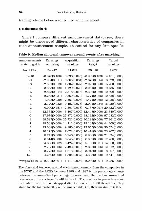
c. Robustness check

Since I compare different announcement databases, theremight be unobserved different characteristics of companies ineach announcement sample. To control for any firm-specific


Table 9. Median abnormal turnover around events after matching

Announcements Earnings Acquisition Earnings Targetmatchingwith acquiring earnings target earnings

No.of Obs. 34,942 11,024 30,618 4,877

t=-10 -0.870(0.106) 0.396(0.045) -0.939(0.103) 4.451(0.000)-9 -2.904(0.011) 0.363(0.064) -2.670(0.014) 3.028(0.000)-8 -2.801(0.019) 1.302(0.027) -2.026(0.050) 5.760(0.000)-7 -3.353(0.008) 1.129(0.029) -3.061(0.010) 9.435(0.000)-6 -2.843(0.014) 2.318(0.015) -2.306(0.029) 10.898(0.000)-5 -2.288(0.031) 0.369(0.070) -1.774(0.065) 10.858(0.000)-4 -1.948(0.039) 2.561(0.005) -1.421(0.068) 12.938(0.000)-3 -2.120(0.032) 0.452(0.076) -2.041(0.034) 16.920(0.000)-2 0.000(0.457) 2.301(0.013) 0.137(0.097) 20.522(0.000)-1 12.335(0.000) 6.407(0.000) 12.448(0.000) 23.740(0.000)0 47.979(0.000) 27.872(0.000) 48.162(0.000) 97.082(0.000)1 39.587(0.000) 25.721(0.000) 40.299(0.000) 77.261(0.000)2 19.538(0.000) 14.211(0.000) 19.134(0.000) 44.409(0.000)3 13.008(0.000) 9.185(0.000) 13.655(0.000) 30.574(0.000)4 10.175(0.000) 7.072(0.000) 10.418(0.000) 23.207(0.000)5 8.741(0.000) 5.946(0.000) 8.936(0.000) 21.624(0.000)6 6.014(0.000) 6.045(0.000) 6.389(0.000) 17.266(0.000)7 4.656(0.002) 3.424(0.007) 5.100(0.001) 14.350(0.000)8 2.738(0.006) 2.480(0.013) 2.860(0.006) 12.512(0.000)9 3.775(0.004) 1.613(0.042) 3.913(0.003) 8.907(0.000)

t=10 4.260(0.000) 1.394(0.037) 4.333(0.000) 9.541(0.000)

Average of t=[-10, -3] -2.391(0.001) 1.111(0.003) -2.030(0.001) 9.286(0.000)

The abnormal turnover around each announcement from the companies inthe NYSE and the AMEX between 1986 and 1997 is the percentage changebetween the annualized percentage turnover and the median annualizedpercentage turnover from t = –40 to t = –11. The p-values in parentheses areestimated from the bootstrapped distribution with 1000 iterations. Theystand for the tail probability of the smaller side, i.e., their maximum is 0.5.


Tab

le 1

0. R

obust

nes

s ch

eck

Pan

el A

: U

sin

g la

rger

est

imat

ion

win

do(

t=–5

5to

-11)

An

nou

nce

men

tE

arn

ings

Acq

uir

ing

Tar

get

No.

of O

bs.

42,7

76

14,9

67

10,0

07

t=[-

10, -3

]-3

.107+

1.3

14*

15.3

37*

-2-0

.047

2.9

56*

28.3

50*

-110.6

13*

6.8

91*

35.5

56*

047.3

55*

29.9

88*

143.4

50*

139.6

79*

26.8

43*

125.6

80*

219.4

73*

14.8

39*

75.1

46*

t=[3

, 10]

6.2

69*

5.3

27*

31.9

82*

Pan

el B

: U

sin

g m

ean

abn

orm

al log

(tu

rnov

er)

An

nou

nce

men

tE

arn

ings

Acq

uir

ing

Tar

get

No.

of O

bs.

37,6

75

13,3

07

8,2

39

t=[-

10, -3

]-1

.741+

2.5

27*

17.0

03*

-21.6

37*

5.1

94*

27.8

00*

-111.9

84*

7.8

30*

34.9

98*

041.1

18*

30.4

75*

99.2

02*

135.7

12*

26.0

63*

92.5

20*

219.3

55*

16.0

86*

62.2

69*

t=[3

, 10]

7.5

58*

5.8

71*

30.4

15*

Pan

el C

: U

sin

g su

b-p

erio

dA

nn

oun

cem

ent

Ear

nin

gsA

cqu

irin

gTar

get

Su

bper

iod

1986-8

91990-9

31994-9

71986-8

91990-9

31994-9

71986-8

91990-9

31994-9

7N

o. o

f O

bs.

10,6

16

12,3

85

18,5

59

3,5

34

3,9

19

7,6

07

4,6

14

2,0

88

3,3

54

t=[-

10, -3

]-1

.260**

-1.9

63+

-3.3

66+

4.2

30*

-0.7

80++

+0.5

74**

24.0

15*

5.8

28*

7.4

60*

-26.8

29*

0.6

91**

*-3

.659+

5.7

87*

0.3

40**

*2.6

66*

44.5

61*

13.2

55*

15.3

54*

-129.9

99*

14.2

86*

0.7

57**

*11.2

45*

4.4

42*

5.9

94*

60.0

00*

12.8

93*

21.9

62*

030.5

04*

53.6

69*

54.4

30*

35.6

46*

21.9

63*

30.3

05*

233.1

00*

79.5

71*

94.0

84*

119.6

99*

40.5

23*

52.4

74*

33.3

33*

21.8

51*

25.3

78*

221.7

40*

60.5

12*

82.6

04*

210.0

96*

23.9

52*

22.6

81*

20.1

65*

10.5

40*

13.8

93*

128.4

10*

33.3

33*

48.5

19*

t=[3

, 10]

4.0

46*

8.5

75*

7.1

25*

8.0

89*

2.2

52*

4.8

79*

51.4

20*

10.6

73*

20.3

08*

For

the

abno

rmal

trad

ing

volu

me,

exc

ept f

or p

anel

B w

here

log(

turn

over

) and

mea

n ab

norm

al tu

rnov

er a

re u

sed,

the

med

ian

turn

over

in th

e es

timat

ion

perio

d(45

day

s in

pan

el A

and

30

days

in p

anel

C) i

s ca

lcul

ated

and

sub

trac

ted

from

the

tur

nove

r in

the

eve

nt w

indo

w. T

he t

urno

ver

is a

n an

nual

ized

and

per

cent

age

num

ber

of t

radi

ng v

olum

e di

vide

d by

sha

res

outs

tand

ing.

Inpa

nel A

and

C, +

++, +

+, a

nd +

mea

n re

spec

tivel

y 10

%, 5

%, a

nd 1

% in

the

left

tail

of t

he b

oots

trap

ped

dist

ribut

ion.

***

, **,

and

* m

ean

resp

ectiv

ely

10%

, 5%

, and

1%

in t

he r

ight

tai

l of t

hebo

otst

rapp

ed d

istr

ibut

ion.

In p

anel

B, +

++, +

+, +

, ***

, **,

and

* are

from

the

t-di

strib

utio

n.

characteristics, I match companies in the earningsannouncement sample and in the acquiring or the targetannouncement sample. However, the result from the matchingsample shows a stronger pattern of decreasing trading volumeonly before an earnings announcement, as in Table 9. Beforematching, the average of the median abnormal turnover from t =–10 to t = –3 is –2.281%. It is slightly increased to –2.391% whenthe data are matched with the acquiring announcement sampleand slightly decreased into –2.030% when the data are matchedwith the target announcement sample.

For the normal level of turnover, the estimation window in thispaper is the period from t = –40 to t = –11. As a robustnesscheck, I attach a summarized table in Panel A of Table 10 from alonger estimation window from t = –55 to t = 11. In this table,the result is greatly strengthened, with –3.107% decrease fromthe normal level of turnover.

Another robustness check involves the use of median and thebootstrapped distribution. In Panel B of Table 10, I apply aconventional approach of an event study where the meanabnormal measure and the t-distribution are used.17) Thedifference of the natural log of turnover and the natural log ofthe normal level turnover is statistically significantly negativeonly before an earnings announcement.

As a robustness check of the stability of this specific pattern, Iprovide the subperiod results in Panel C of Table 10. Amongthree subperiods, only in the earliest period of 1986-1989, thesignificance level is 5%. In the other two subperiods, the medianabnormal turnover is decreased around 2-3% with less than 1%significance level. Before either an acquiring or a targetannouncement, I do not observe this interesting and intuitivetrading volume pattern.

5. Conclusion

Using the I/B/E/S earnings announcement and the SDC


17) In order to deal with the skewness of turnover, I use the natural log. Becausethere are many zero turnovers in the sample, I use the negative value of themaximum of log(turnover) for the value of log(zero turnover). This will makethe entire distribution almost symmetric.

takeover announcement data from 1986 to 1997, I find that thedecreasing trading volume exists only before a scheduledearnings announcement. Constructing a simple and intuitivemodel, this interesting pattern of trading volume can beexplained as resulting from the information asymmetry and thetrading behavior of discretionary liquidity traders. I relate thetrading volume pattern with proxies of the ex ante informationasymmetry. The proxies such as analyst coverage, size, andindustry categorization are all correspondingly related with thetrading volume only before a scheduled announcement.However, between analyst coverage and size, analyst coverageshows a clearer cross-sectional relationship with the tradingvolume pattern.

I investigate the trading volume and risk measures(volatilityand risk) to differentiate two possible explanations of thedecreasing trading volume: the information asymmetryexplanation vs. the risk-based explanation. The result from theinvestigation of risk measures excludes the latter explanation.Also, following the logic of the model, the absolute return dividedby turnover(a measure of price sensitivity) increases only beforean earnings announcement; this makes the informationasymmetry explanation, as in the model, much more plausible.

The robustness of the methodologies in this study has beencarefully probed, and I believe that I have shown aneconomically intuitive trading volume pattern to be related toanother kind of hitherto unexplored information, the timinginformation. Even with different estimation windows, meanabnormal log turnover, and varying sub-periods, the main resultof this paper is preserved. Unlike most anomalies in financialeconomics, this specific pattern seems to be even morepronounced in recent sub-periods.

I conclude that the timing information provides discretionaryliquidity traders with an opportunity for trading optimizationunder information asymmetry and that this causes a decrease oftrading volume only before a scheduled announcement. Tworemaining questions of interest, the return implication of thistiming information asymmetry and the identification of escapingtraders using a specific data set, will be explored in my furtherresearch in progress.


Appendix

Since the current model is a modified model from Admati andPfleiderer(1988) or Kyle(1984, 1985), so my notation conformswith that in Admati and Pfeiderer(1988) or Kyle(1984, 1985).

Proof of Lemma 1

To calculate the aggressiveness of trading by informed traders(β) and the price sensitivity to the order flow of the market maker(λ), we need to use two conditions; informed traders’ expectedprofit maximization and the market maker’s zero profitcondition.

For the informed traders’ decision, they will maximize theexpected profits,

where

and (A1)

(A2)

The ith informed investor will conjecture the market order ofother N – 1 informed traders as β(δ + ε ). Therefore, the totalorder flow is xi + (N – 1)β( δ + ε ) + y + z. So, ith informed investorswill choose xi to maximize

(A3)

To maximize this, xi is set to equal to

(A4)VarVar Var

N[ ]( [ ] [ ])

( )( ˜ ˜)

δλ δ ε

β δ ε2

12+

− −

+

E x x N y zi i[ ( ˜ ( ( ) ( ˜ ˜) ˜ ˜))| ˜ ]δ λ β δ ε δ ε− + − + + + +1

E x x y zi ii

N

[ ( ˜ ( ˜ ˜))| ˜ ]δ λ δ ε− + + +=∑

1

˜ ˜ ˜ ˜Ω = + +=∑ x y zii

N

1

P E F w F w w x y zii

N

( ˜ ) [ ˜] ˜ ˜, ˜ ˜ ˜Ω = + = + = + +=∑λ λ

1

E x F Pi[ ( ˜ ( ˜ ))| ˜ ]− +Ω δ ε


Since this should be equal to β(δ + ε), the aggressiveness ofinformed traders (β) will be

(A5)

The information set for informed investors is a noisy signal (δ +ε) and the conditional expectation of the order flow of DLT andNLT are zero on this signal, so the profits maximization forinformed traders will not be changed from an unscheduledannouncement case to scheduled announcement case. However,the market maker’s pricing problem will be changed since herinformation set is order flow (w). The investigation for anunscheduled announcement case, a benchmark case, and ascheduled announcement case follows.

First, before unscheduled announcements, discretionaryliquidity traders cannot behave as discretionary liquidity traders(y) since they cannot detect an incoming announcement, theywill behave as naive traders (z ). Therefore, the market maker’sobserved order flow will be

(A7)

In a competitive market making industry, the expected profitshould be zero. This implies

(A8)

So, the price sensitivity of order flow (λ) will be decided bycovariance of dividend in the future and order flow and varianceof order flow.

(A9)λ β δβ δ ε

U N Var

N Var Var Var y Var z=

+ + +[ ˜]

( [ ˜] [ ]) [ ˜] [ ˜]2 2

P E F w E F w F

Cov wVar w

w( ˜ ) [ ˜] ˜ [ ˜| ˜ ][ , ˜ ][ ˜ ]

˜Ω = + = = +λ δ

˜ ˜ ˜w x y zii

N

= + +=∑

1

β δλ δ ε

=+ +

Varn Var Var

[ ]( )( [ ] [ ])1


With (A5) and (A9), the unique and positive price sensitivity oforder flow (λ) is found in a third order equation as (A10).

(A10)

Once the price sensitivity to order flow (λ) for an unscheduledannouncement case is found, the trading aggressiveness ofinformed traders (β) will be as in (A11).

(A11)

Second, as a benchmark case, if there are initially nodiscretionary liquidity traders (so, no y in the model), there willbe only naive liquidity traders (z ). This case can be understoodas the case with the lowest liquidity in the market.

With similar informed traders’ profit maximization problemand the market maker’s zero profit condition, the pricesensitivity to order flow (λ) and the trading aggressiveness ofinformed traders (β) will be (A12) and (A13), respectively.

(A12)

(A13)

Third, with a scheduled announcement, the market maker willconsider the existence of discretionary liquidity traders whenshe decides the price. Therefore, the market maker’s observedorder flow will be

(A14)˜ ˜ ˜w x y zii

N

= + −

+=∑

1

λ λλ

βδ ε

=+

Var z

N Var Var

[ ˜]

( [ ˜] [ ])

λ δ

δ ε=

+ +VarN

N

Var Var Var z

[ ˜]( ) ( [ ˜] [ ] [ ˜]1

β

δ εU Var y Var z

N Var Var= +

+[ ˜] [ ˜]

( [ ˜] [ ])

λ δδ ε

U VarN

N

Var Var Var y Var z=

+ + +[ ˜]

( ) ( [ ˜] [ ]( [ ˜] [ ˜])1


In (A14), DLT’s react to the price sensitivity from the marketmaker, since they know there will be an upcomingannouncement and they are keen to the movement of the pricein the market. So, when the price sensitivity is zero, they willtake part in the market as they do before an unscheduledannouncement. However, as the price sensitivity increases, theywill participate in the market less and less. When the pricesensitivity is the same as that of the bench mark case (i.e. thehighest possible price sensitivity in the market), all DLT’s willescape from the market.

With order flow information as in (A14), the market maker willdecide the price as in (A15)

(A15)

So, the price sensitivity of order flow (λ) will be decided bycovariance of dividend in the future and order flow and varianceof order flow.

(A16)

With (A5) and (A16), the unique and positive price sensitivityof order flow (λ) is found in a fourth order equation as (A10) withreasonable values of parameters (i.e. Var[y ] ≤ 8∙Var[z ]).

(A17)

Once the price sensitivity to order flow (λ) for an unscheduledannouncement case is found, the trading aggressiveness ofinformed traders (β) will be as in (A11).

(A18)

Q.E.D.

β βδ ε

S Var z

N Var Var= =

+[ ˜]

( [ ˜] [ ])

λ λ δδ ε

S VarN

N

Var Var Var z= =

+ +[ ˜]

( ) ( [ ˜] [ ]) [ ˜]1

λ β δ

β δ ε λ λλ

S N Var

N Var Var Var y Var z

=

+ + +

+

[ ˜]

( [ ˜] [ ]) [ ˜] [ ˜]2 22

P E F w E F w F

Cov wVar w

w( ˜ ) [ ˜] ˜ [ ˜| ˜ ][ , ˜ ][ ˜ ]

˜Ω = + = = +λ δ


Reference

Abraham, A. and W. M. Taylor, 1997, A scheduled event option pricingmodel, Review of Quantitative Finance and Accounting 8, 152-162.

Admati, A. and P. Pfleiderer, 1988, A theory of intraday patterns:Volume and price variability, Review of Financial Studies 1, 3-40.

Atiase, R. and L. S. Bamber, 1994, Trading volume reactions to annualaccounting earnings announcements, Journal of Accounting andEconomics 17, 309-329

Bamber, Linda Smith, 1987, Unexpected earnings, firm size, andtrading volume around quarterly earnings announcements,Accounting Review 62, 510-532.

Bamber, L. and Y. Cheon, 1995, Differential price and volume reactionsto accounting earnings announcements, The Accounting Review70, 417-441.

Barclay, M. J., R. H. Litzenberger, and J. B. Warner, 1990, PrivateInformation, Trading Volume, and Stock-Return Variances, Reviewof Financial Studies 3, 233-253.

Chordia, T., A. Subrahmanyam, and V. R. Anshuman, 2001, Tradingactivity and expected stock returns, Journal of FinancialEconomics 59, 3-32.

Dimson, Elroy, 1979, Risk measurement when shares are subject toinfrequent trading, Journal of Financial Economics 7, 197-226.

Donders, M. and T. Vorst, 1996, The impact of firm specific news onimplied volatilities, Journal of Banking and Finance 20, 1447-1461.

Ederington, L. H. and J. H. Lee, 1993, How markets processinformation: News releases and volatility, Journal of Finance 48,1161-1191.

Efron, B., and R. Tibshirani, 1983, An introduction to the bootstrap,Chapman and Hall, New York, New York.

Foster, F.D. and S. Viswanathan, 1990, A theory of the interdayvariations in volume, variance, and trading costs in securitiesmarkets, Review of Financial Studies 3, 593-624.

Foster, G., C. Olsen, and T. Shevlin, 1984, Earnings Releases,anomalies, and the behavior of security returns, The AccountingReview 59, 574-603.

Gallant, A. R., P. E. Rossi, and G. Tauchen, 1992, Stock Prices andVolume, Review of Financial Studies 5, 199-242.

Gervais, Simon, R. Kaniel and D. Mingelgrin, 2000, The High VolumeReturn Premium, Journal of Finance 56, 877-919.


He, H. and J. Wang, 1995, Differential Information and DynamicBehavior of Stock Trading Volume, Review of Financial Studies 8,919-972.

Hong, H., T. Lim, and J. Stein, 1998, Bad news travels slowly: Size,analyst coverage and the profitability of momentum strategies,NBER working paper 6553.

Jarrell, Gregg, and Annette Poulsen, 1989, Returns to acquiring firmsin tender of fers: Evidence from three decades, FinancialManagement 18, 12-19.

Jayaraman, N., M. B. Frye, and S. Sabherwal, 2001, Informed tradingaround merger announcements: An empirical test usingtransaction volume and open interest in potions market, FinancialReview May (Symposium Issue).

Jensen, Michael C., and Richard Ruback, 1983, The market forcorporate control: The scientific evidence, Journal of FinancialEconomics 11, 5-50.

Karpoff, Jonathan, 1987, The Relation between Price Changes andTrading Volume: A Survey, Journal of Financial and QuantitativeAnalysis 22, 109-126.

Kim, O. and R. E. Verrecchia, 1991a, Trading volume and pricereactions to public announcements, Journal of AccountingResearch 29, 302-321.

Kim, O. and R. E. Verrecchia, 1991b, Market reaction to anticipatedannouncements, Journal of Financial Economics 30, 273-309.

Kim, O. and R. E. Verrecchia, 1994, Market liquidity and volumearound earnings announcements, Journal of Accounting andEconomics 17, 41-67.

Kyle, Albert, 1985, Continuous Auctions and Insider Trading,Econometrica 53, 1315-1336.

Lee, Charles M. C. and B. Swaminathan, 2000, Price Momentum andTrading Volume, Journal of Finance 55, 2017-2069.

Lewellen, Jonathan, 1999, The time-series relations among expectedreturn, risk, and book-to-market, Journal of Financial Economics54, 5-43.

Li, L and R. F. Engle, 1998, Macroeconomic announcements andvolatility of treasury futures, Working Paper, University ofCalifornia, San Diego.

Lo, A. W. and J. Wang, 2000, Trading Volume: Definitions, DataAnalysis, and Implications of Portfolio Theory, Review of FinancialStudies, 13, 257-300.

Lo, A. W. and J. Wang, 2001, Stock Market Trading Volume, WorkingPaper, MIT.

Sanders, R. W. Jr. and J. S. Zdanowicz, 1992, Target Firm Abnormalreturns and Trading Volume around the Initiation of Change in


Control Transactions, Journal of Financial and QuantitativeAnalysis 27, 109-129.

Shalen Catherine T., 1993, Volume, Volatility, and the Dispersion ofBeliefs, Review of Financial Studies 6, 405-434.

Wang, Jiang, 1994, A model of competitive stock trading volume,Journal of Political Finance 102, 127-168.


escape from the market: discretionary liquidity trading

Documents