esl users guide interim final 22feb16 · pdf file16.02.2016 · february 2016 esl...
TRANSCRIPT


February 2016 ESL User’s Guide
For Comments and Questions, Please Contact: Email: [email protected]
‐or‐
Nicole Fry, Ph.D
San Francisco Bay Regional Water Quality Control Board
1515 Clay Street, Suite 1400
Oakland, CA 94612
Phone: 1‐510‐622‐5047
DISCLAIMER
This User’s Guide: Derivation and Application of Environmental Screening Levels
(2016) is a technical report prepared by staff of the California Regional Water
Quality Board, San Francisco Bay Region (Regional Water Board staff). This
User’s Guide is not intended to establish policy or regulation. The Environmental
Screening Levels (ESLs) presented in this User’s Guide and the accompanying
tables (Excel spreadsheets) are specifically not intended to serve as:
a stand‐alone decision making tool,
guidance for the preparation of baseline environmental assessments,
a rule to determine if a waste is hazardous under the state or federal
regulations, or
a rule to determine when the release of hazardous chemicals must be
reported to the overseeing regulatory agency.
Also, in general, the ESLs are not used at sites that are subject to the Low‐Threat
Underground Storage Tank Closure Policy (State Water Board 2012b). They may be
used at such sites to screen for constituents not already addressed by the Policy
or as part of site‐specific risk assessments for the media‐specific criteria (e.g.,
Groundwater; Petroleum Vapor Intrusion to Indoor Air; and Direct Contact and
Outdoor Air).
ESLs may not be adequately protective for some sites. For example, they should
not be used at sites where physical conditions or exposure scenarios substantially
differ from those assumed in development of the ESLs. In addition, the ESLs do
not apply to sediment or sensitive ecological habitats (such as wetlands or
endangered‐species habitats). The need for a detailed human health or ecological
risk assessment should be evaluated on a site‐by‐site basis for areas where
significant concerns may exist.

February 2016 ESL User’s Guide
Use of the ESLs by dischargers or regulators is optional. Dischargers seeking to
use the ESLs at their sites should discuss this with the overseeing regulatory
agency. The presence of a chemical at concentrations in excess of an ESL does not
necessarily indicate adverse effects on human health or the environment, rather
that additional evaluation is warranted. Use of the ESLs as cleanup goals should be evaluated in view of the overall site investigation results and the cost/benefit
of performing a more site‐specific evaluation. Lastly, the ESLs should not be
used as criteria to determine when chemical concentrations at a site must be
reported to a regulatory agency.
The information presented in this document is not final Board action. Regional
Water Board staff reserves the right to change this information at any time
without public notice. This document is not intended, nor can it be relied upon,
to create any rights enforceable by any party in litigation in the State of
California. Staff in overseeing regulatory agencies may decide to follow the
information provided herein or act at a variance with the information, based on
an analysis of site‐specific circumstances.
This document will be periodically updated as needed. Regional Water Board
staff overseeing work at a specific site should be contacted prior to use of this
document in order to ensure that the document is applicable to the site and that
the user has the most up‐to‐date version available. This document is not
copyrighted. Copies may be freely made and distributed. Reference to the ESLs
without adequate review of the User’s Guide could result in misinterpretation
and misuse of the ESLs.
February 2016 ESL User’s Guide
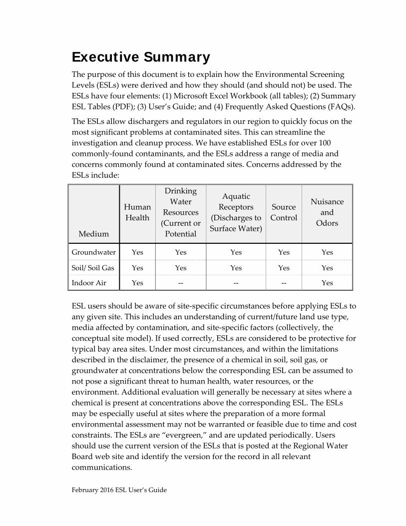
Executive Summary The purpose of this document is to explain how the Environmental Screening
Levels (ESLs) were derived and how they should (and should not) be used. The
ESLs have four elements: (1) Microsoft Excel Workbook (all tables); (2) Summary
ESL Tables (PDF); (3) User’s Guide; and (4) Frequently Asked Questions (FAQs).
The ESLs allow dischargers and regulators in our region to quickly focus on the
most significant problems at contaminated sites. This can streamline the
investigation and cleanup process. We have established ESLs for over 100
commonly‐found contaminants, and the ESLs address a range of media and
concerns commonly found at contaminated sites. Concerns addressed by the
ESLs include:
Medium
Human
Health
Drinking
Water
Resources
(Current or
Potential
Aquatic
Receptors
(Discharges to
Surface Water)
Source
Control
Nuisance
and
Odors
Groundwater Yes Yes Yes Yes Yes
Soil/ Soil Gas Yes Yes Yes Yes Yes
Indoor Air Yes ‐‐ ‐‐ ‐‐ Yes
ESL users should be aware of site‐specific circumstances before applying ESLs to
any given site. This includes an understanding of current/future land use type,
media affected by contamination, and site‐specific factors (collectively, the
conceptual site model). If used correctly, ESLs are considered to be protective for
typical bay area sites. Under most circumstances, and within the limitations
described in the disclaimer, the presence of a chemical in soil, soil gas, or
groundwater at concentrations below the corresponding ESL can be assumed to
not pose a significant threat to human health, water resources, or the
environment. Additional evaluation will generally be necessary at sites where a
chemical is present at concentrations above the corresponding ESL. The ESLs
may be especially useful at sites where the preparation of a more formal
environmental assessment may not be warranted or feasible due to time and cost
constraints. The ESLs are “evergreen,” and are updated periodically. Users
should use the current version of the ESLs that is posted at the Regional Water
Board web site and identify the version for the record in all relevant
communications.

February 2016 ESL User’s Guide i
TABLE OF CONTENTS
EXECUTIVE SUMMARY ............................................................................ ES-1
1 INTRODUCTION AND BACKGROUND ................................................. 1-1
1.1 San Francisco Bay Basin Water Quality Control Plan (Basin Plan) ......... 1‐3
1.1.1 Beneficial Uses of Surface Water and Groundwater .................... 1‐4
1.1.2 Environmental Concerns in the Basin Plan ................................... 1‐5
1.1.3 Investigation and Cleanup of Discharges ...................................... 1‐6
1.2 Comparison of ESLs to Other Screening Levels and Criteria .................. 1‐7
1.2.1 Other Screening Levels ..................................................................... 1‐7
1.2.2 Hazardous Waste Regulations and OSHA Standards ................. 1‐9
1.2.3 OSHA Standards: Permissible Exposure Limits ......................... 1‐10
1.3 Site Closure Evaluations: Use of the ESLs ................................................ 1‐12
1.3.1 Low‐Threat Underground Storage Tank Case Closure Policy . 1‐13
1.3.2 Closure Criteria for Non‐UST Sites .............................................. 1‐14
2 STEP-BY-STEP GUIDE: ESL WORKBOOK ............................................ 2-1
2.1 Conceptual Site Model................................................................................... 2‐2
2.2 ESL Workbook Content ................................................................................. 2‐8
2.3 Tier 1 ESLs – Default Conservative Site Scenario ...................................... 2‐9
2.4 Tier 2 ESLs – Site Specific ESL Choice and Use of Interactive Tool ...... 2‐10
Step 1: Check ESL Applicability and Updates ......................................... 2‐10
Step 2: Identify Chemicals of Potential Concern ...................................... 2‐11
Step 3: Land Use Selection .......................................................................... 2‐11
Step 4: Groundwater Use Selection ........................................................... 2‐12
Step 5: MCL Priority vs Risk‐Based Screening Levels Selection ............ 2‐13
Step 6: Groundwater Depth Selection ....................................................... 2‐13
Step 7: Soil Type Selection ........................................................................... 2‐14
Step 8: Soil Exposure Depth Selection ....................................................... 2‐14
Step 9: Final ESL Determination Process .................................................. 2‐15

February 2016 ESL User’s Guide ii
Step 10: Compare Site Data to ESLs ........................................................... 2‐19
Step 11: Compare Site Data to Background Levels ................................. 2‐19
Step 12: Evaluate the Need for Additional Investigation, Assessment, or
Remediation ..................................................................................... 2‐20
Example of Interactive Tool Use: Tetrachloroethene .............................. 2‐20
2.5 Tier 3 ‐ Risk Assessment Derived Screening Levels ................................ 2‐24
3 METHODS: DIRECT EXPOSURE HUMAN HEALTH RISK SCREENING LEVELS FOR ALL MEDIA ..................................................................... 3-1
3.1 Default Exposure Scenarios: Receptors and Pathways ............................. 3‐1
Residents .......................................................................................................... 3‐1
Commercial or Industrial Workers .............................................................. 3‐1
Construction Workers .................................................................................... 3‐2
3.2 Calculation of Health Risk‐Based Exposure Screening Levels ................ 3‐3
3.2.1 Toxicity Values .................................................................................. 3‐3
3.2.2 Exposure Factors ............................................................................... 3‐5
3.2.3 Equations for Health Risk‐Based Screening Levels Considering a
Single Chemical ................................................................................. 3‐1
3.2.4 Cumulative Risk Considering Multiple Chemicals ...................... 3‐5
3.2.5 Groundwater Specific Exposure Considerations .......................... 3‐6
3.3 Other Human Health Risk Criteria .............................................................. 3‐6
3.4 Exceptions ....................................................................................................... 3‐7
3.4.1 MCL Priority ...................................................................................... 3‐7
3.4.2 Lead ..................................................................................................... 3‐8
3.4.3 Short‐Term Exposure Levels: Trichloroethene ............................. 3‐8
3.4.4 Chemical Mixtures ............................................................................ 3‐9
3.5 Site‐Specific Evaluations ............................................................................. 3‐10
4 METHODS: VAPOR INTRUSION RISK SCREENING LEVELS FOR GROUNDWATER AND SUBSLAB/SOIL GAS ........................................ 4-1
4.1 Background ..................................................................................................... 4‐1
4.1.1 Conceptual Model for Vapor Intrusion into Buildings ................ 4‐1
4.1.2 CVOC Vapor Intrusion versus Petroleum Vapor Intrusion........ 4‐2

February 2016 ESL User’s Guide iii
4.1.3 Approaches to Evaluating Vapor Intrusion .................................. 4‐3
4.2 Attenuation Factors for Vapor Intrusion .................................................... 4‐4
4.2.1 Development of Soil Gas Attenuation Factors .............................. 4‐5
4.2.2 Development of Groundwater Attenuation Factors .................... 4‐6
4.2.3 Site‐Specific Attenuation Factors for Vapor Intrusion ................. 4‐8
4.3 TCE Vapor Intrusion Trigger Levels for Indoor Air Sampling ............... 4‐9
5 METHODS: ECOTOXICITY AQUATIC HABITAT SCREENING LEVELS FOR GROUNDWATER ................................................................................. 5-1
5.1 Aquatic Receptor Toxicity Criteria .............................................................. 5‐1
5.2 Exceptions ....................................................................................................... 5‐3
5.3 Site‐Specific Evaluations ............................................................................... 5‐3
6 METHODS: LEACHING TO GROUNDWATER SCREENING LEVELS FOR SOIL .................................................................................................... 6-1
6.1 Calculation of Soil Leaching Screening Levels ........................................... 6‐1
6.1.1 Specific Model Calculation Inputs .................................................. 6‐2
6.2 Exceptions ....................................................................................................... 6‐4
6.2.1 Pentachlorophenol and Bis(2‐ethylhexyl)phthalate ..................... 6‐4
6.2.2 Polychlorinated Biphenyls (PCBs) .................................................. 6‐4
6.2.3 Perchlorate .......................................................................................... 6‐4
6.3 Site‐Specific Evaluations ............................................................................... 6‐5
7 METHODS: GROSS CONTAMINATION SCREENING LEVELS FOR GROUNDWATER AND SOIL................................................................. 7-1
7.1 Media Specific Gross Contamination Approach ....................................... 7‐1
7.2 Exception: Total Petroleum Hydrocarbon Mixtures ................................. 7‐1
8 METHODS: TASTE AND ODOR NUISANCE SCREENING LEVELS FOR ALL MEDIA ................................................................................................. 8-1
8.1 Groundwater Taste and Odor Nuisance Levels ........................................ 8‐1
8.1.1 Groundwater: Drinking Water Resource ....................................... 8‐1
8.1.2 Groundwater: Non‐Drinking Water Resources ............................ 8‐2
8.2 Soil Odor Nuisance Levels ............................................................................ 8‐2
8.3 Indoor Air and Soil Gas Odor Nuisance Levels ......................................... 8‐3

February 2016 ESL User’s Guide iv
9 METHODS: CHEMICAL MIXTURES OR GROUPS ................................. 9-1
9.1 Chlordane ........................................................................................................ 9‐1
9.2 DDD, DDE, and DDT .................................................................................... 9‐1
9.3 Dioxins and Furans ........................................................................................ 9‐2
9.4 Endosulfan ...................................................................................................... 9‐4
9.5 Polychlorinated Biphenyls (PCBs) ............................................................... 9‐4
9.6 Polycyclic Aromatic Hydrocarbons (PAHs) ............................................... 9‐5
9.7 Total Petroleum Hydrocarbons (TPH) ........................................................ 9‐7
9.7.1 Risk and Hazard Evaluation for Petroleum Hydrocarbon
Releases ............................................................................................... 9‐7
9.7.2 Fraction Approach for Human Health Risk TPH ESLs ............... 9‐9
9.7.3 Petroleum Degradates .................................................................... 9‐10
9.7.4 Laboratory Analysis for Use with TPH ESLs .............................. 9‐14
10 ADDITIONAL CONSIDERATIONS ..................................................... 10-1
10.1 Laboratory Data Issues ................................................................................ 10‐1
10.1.1 Detection Limits and Reporting Limits ........................................ 10‐1
10.1.2 Soil Data Reporting: Dry Weight Basis ........................................ 10‐1
10.2 Naturally Occurring Background and Ambient Chemicals................... 10‐2
10.3 Bioavailability ............................................................................................... 10‐3
10.4 Degradation Products .................................................................................. 10‐3
10.5 Chemical Specific Considerations .............................................................. 10‐4
10.5.1 Chemicals Not Listed In ESLs ....................................................... 10‐4
10.5.2 Multiple Species of One Chemical ................................................ 10‐4
10.5.3 Arsenic .............................................................................................. 10‐5
10.5.4 Cadmium .......................................................................................... 10‐5
10.6 Acute Hazards: Methane ............................................................................. 10‐5
10.7 Sediment ........................................................................................................ 10‐6
10.8 Total Maximum Daily Loads (TMDLs) ..................................................... 10‐8

February 2016 ESL User’s Guide v
11 ACKNOWLEDGEMENTS ..................................................................... 11-1
12 REFERENCES ..................................................................................... 12-1
13 ACRONYMS AND ABBREVIATIONS ................................................... 13-1
FIGURES Figure 2‐1 – Tiered Process for Selecting Screening Levels .................................... 2‐1
Figure 2‐2 – Example Illustrating Extent of Tetrachloroethene in Shallow
Groundwater ........................................................................................... 2‐4
Figure 2‐3 – Example Cross Section Illustrating Contaminant Migration ............ 2‐5
Figure 2‐4 – Default Evaluation of Receptors and Exposure Pathways Used in a
Tier 1 Assessment ................................................................................... 2‐6
Figure 2‐5 – Example of a Site‐Specific Evaluation of Receptors and Exposure
Pathways .................................................................................................. 2‐7
Figure 2‐6 – Final Site‐Specific Groundwater ESL Determination ...................... 2‐16
Figure 2‐7 – Final Site‐Specific Soil ESL Determination ........................................ 2‐17
Figure 2‐8 – Final Site‐Specific Subslab/ Soil Gas ESL Determination ................ 2‐18
Figure 2‐9 – Final Site‐Specific Indoor Air ESL Determination ............................ 2‐18
Figure 2‐10 – Interactive Tool ESL Workbook Site Specific Inputs Table T2‐1
based on the example scenario described herein ............................. 2‐22
Figure 2‐11 – Interactive Tool ESL Workbook Details Table T2‐2 for PCE ESLs
based on the example scenario described herein ............................. 2‐23
Figure 2‐12 – Interactive Tool ESL Workbook Specific Concerns Table T2‐3 based
on the example scenario described herein ........................................ 2‐24
TABLES Table 1‐1 – Regional Water Board Technical Resource Documents for Use with
the ESLs ..................................................................................................... 1‐1
Table 1‐2 – Environmental Concerns Stated or Implied in the Basin Plan ........... 1‐6
Table 1‐3 – Environmental Concerns in the ESLs versus Other Screening Levels 1‐
8

February 2016 ESL User’s Guide vi
Table 1‐4 – Low‐Threat UST Closure Policy General Criteria .............................. 1‐13
Table 1‐5 – Regional Water Board Closure Criteria for Non‐UST Sites .............. 1‐14
Table 2‐1 – Information for a Conceptual Site Model .............................................. 2‐2
Table 2‐2 – Tier 1 ESL Conceptual Site Model ........................................................ 2‐10
Table 2‐3 – Soil Direct Exposure Depth Intervals ................................................... 2‐15
Table 3‐1— Exposure Pathways for Each Direct Exposure Medium .................... 3‐2
Table 3‐2 – Toxicity Value Hierarchy ......................................................................... 3‐4
Table 3‐3 – Exposure Factor Selection ........................................................................ 3‐1
Table 3‐4 – Hierarchy for Other Health‐Based Criteria for Drinking Water ........ 3‐7
Table 4‐1 – Vapor Intrusion Approaches ................................................................... 4‐4
Table 4‐2 – Subslab and Soil Gas Attenuation Factors for Concrete Slab‐on‐Grade
Buildings ................................................................................................... 4‐5
Table 4‐3 – Groundwater Vapor Intrusion Scenarios for Existing Residential and
Commercial/Industrial Buildings .......................................................... 4‐7
Table 4‐4 – TCE ESLs, Action Levels for Indoor Air (Response), and
Groundwater and Soil Gas Trigger Levels (Sample Indoor Air) .... 4‐10
Table 5‐1 – Aquatic Receptor Toxicity Value Hierarchy ......................................... 5‐2
Table 6‐1 – Soil Leaching to Groundwater Model Design ...................................... 6‐3
Table 8‐1 – Hierarchy of Taste and Odor Thresholds for Groundwater and
Surface Water ............................................................................................ 8‐1
Table 8‐2 – Criteria for Assignment of Odor Upper Limit Levels for Soil ........... 8‐3
Table 9‐1 – World Health Organization Toxic Equivalency Factors for Dioxins
and Furans (2005) ..................................................................................... 9‐3
Table 9‐2 – PAHs in the ESLs and Interim Toxic Equivalency Factors for the
Carcinogenic PAHs .................................................................................. 9‐6
Table 9‐3 – Example Indicator Compounds for Gasoline, Diesel, and Motor Oil9‐8
Table 9‐4 – Petroleum‐Related Compounds Detected in Extractable TPH Analysis
Based on Stage of Weathering .............................................................. 9‐13
Table 9‐5 – TPH Analysis Approach for Petroleum Releases ............................... 9‐15
Table 10‐1 –Sediment Chemical Criteria or Relevant Guidance .......................... 10‐7

February 2016 ESL User’s Guide vii
APPENDICES A – Tier 3 Risk Assessment Information
B – Technical Resource Document: Default Subslab Soil Gas and Soil Gas to
Indoor Air Attenuation Factors in the ESLs
C – Model Parameters for Groundwater Vapor Intrusion ESLs
D – Recommendations for Site‐Specific Vapor Intrusion Models
E – Manual Calculation of Soil Leaching to Groundwater ESLs
F – Technical Resource Document: Fraction Approach to Develop ESLs for TPH
Mixtures
G – Technical Resource Document: Site‐Specific Evaluation Approach for
Petroleum Degradates

February 2016 ESL User’s Guide 1‐1
1 Introduction and Background
The Environmental Screening Levels (ESLs) are groundwater, soil, soil gas, and
indoor air concentrations developed by San Francisco Bay Regional Water
Quality Control Board (Regional Water Board) staff for over 100 chemicals that
can be directly compared to environmental sample data collected at
contaminated sites. The ESLs consist of the following:
1. ESL Workbook (Microsoft Excel 2010 Workbook);
2. Summary ESL Tables (PDF);
3. User’s Guide; and
4. Frequently Asked Questions (FAQs)
In addition, Table 1‐1 lists associated, stand‐alone technical resource documents
that address specific topics that should be used in conjunction with the ESLs.
Table 1‐1 – Regional Water Board Technical Resource Documents for Use with
the ESLs Year Title
1996 Supplemental Instructions to State Water Board December 8, 1995,
Interim Guidance on Required Cleanup at Low Risk Fuel Sites
2006 Draft Technical Resource Document – Characterization and Reuse of
Petroleum Hydrocarbon Impacted Soil as Inert Waste
2009 Assessment Tool for Closure of Low‐Threat Chlorinated Solvent
Sites
2014
Draft Interim Framework for Assessment of Vapor Intrusion at TCE‐
Contaminated Sites in the San Francisco Bay Region (TCE
Framework)
2016a Technical Resource Document: Default Subslab Soil Gas and Soil Gas
to Indoor Air Attenuation Factors in the ESLs
2016b Technical Resource Document: Fraction Approach to Develop ESLs
for TPH Mixtures
2016c Technical Resource Document: Site‐Specific Evaluation Approach for
Petroleum Degradates

February 2016 ESL User’s Guide 1‐2
The following are key aspects of the ESLs:
The ESLs are intended to be a tool to screen or evaluate the threats posed by contamination at a site.
Sites that are adequately characterized with data all below the ESLs, most likely
do not pose a chemical threat. In some rare instances, there could be an exception
resulting from cumulative risk where a large number of chemicals are detected,
but the concentrations are just below the respective ESL (evaluation of
cumulative risk is discussed in Chapter 3). For a site where chemical
concentrations exceed the ESLs, the site may pose a chemical threat and require
further investigation or evaluation to better assess the threat.
The ESLs are intended to be conservative, but reasonable.
The purpose of screening levels is to enable users to distinguish which sites pose
a significant threat relatively quickly. In developing screening levels, there needs
to be a balance between conservativeness and reasonableness so that low risk
sites are screened out and sites with a significant threat are screened in. When
developing screening levels from models, such as those used for human health
risk criteria, if the most conservative value is used for every input parameter, the
resulting screening level often will be overly conservative. This can cause sites
that pose no significant threat to be screened in, requiring the expenditure of
resources (time and money) by all stakeholders (regulatory, discharger, and
others) to further assess the site. This is inefficient and problematic in that it
diverts resources from sites with significant threats.
The ESLs are a communication tool amongst the various stakeholders.
Screening levels help dischargers, technical consultants, and stakeholders
understand Regional Water Board staff expectations and approaches to
evaluating contaminated sites. The ESLs are not default cleanup goals. Cleanup
goals typically are chemical concentrations for a specific site that are agreed‐
upon through evaluation and discussions between the overseeing regulatory
agency and dischargers considering site‐specific conditions. For many sites, ESLs
are selected as cleanup goals, but only after going through the process of
evaluation and adoption. For initial site cleanup orders, the Regional Water
Board typically uses the ESLs as preliminary cleanup goals until site‐specific
cleanup goals have been developed, often required by an order.

February 2016 ESL User’s Guide 1‐3
The ESLs save time and money.
Preparation of quantitative environmental risk assessments for multiple
pathways at contaminated sites requires a greater level of expertise and
frequently requires a multi‐disciplinary team (toxicologists or risk assessors,
chemists, engineers, environmental scientists, and geologists). The costs for small
businesses and property owners with limited financial resources can be cost‐
prohibitive. A Tier 2 risk evaluation can be developed relatively quickly with the
ESLs.
The ESLs are a prioritization tool.
Regional Water Board staff is required to prioritize our oversight of cases to
maximize our protection of human health and the environment. The ESLs serve
as an aid in assessing overall threat (pathways and threat level) allowing us to
understand whether threats to human health or the environment are controlled.
Then we can prioritize the investigation and cleanup needed to eliminate or
control the threats posed by a site.
1.1 San Francisco Bay Basin Water Quality Control Plan (Basin Plan)
The ESLs were ultimately developed to help the Regional Water Board staff
regulate quality in the Region. By law, the Regional Water Board is required to
develop, adopt (after public hearing), and implement a Water Quality Control
Plan (Basin Plan) for the region (San Francisco Bay Region). The Basin Plan is the
master policy document that contains descriptions of the legal, technical, and
programmatic bases of water quality regulation in the region. The plan includes:
A statement of beneficial water uses to be protected;
The water quality objectives needed to protect the designated beneficial
water uses; and
The strategies and time schedules for achieving the water quality
objectives.
The San Francisco Bay Region is 4,603 square miles, roughly the size of the State
of Connecticut, and characterized by its dominant feature, 1,100 square miles of
the 1,600 square mile San Francisco Bay Estuary (Estuary), the largest estuary on
the west coast of the United States, where fresh waters from California’s Central

February 2016 ESL User’s Guide 1‐4
Valley mix with the saline waters of the Pacific Ocean (Regional Water Board
2013).
Because of its highly dynamic and complex environmental conditions, the Bay
system supports an extraordinarily diverse and productive ecosystem. Within
each section of the Bay, there are deepwater areas adjacent to large expanses of
very shallow water. Salinity levels range from hypersaline to fresh water, and
water temperature varies throughout the Bay system. These factors greatly
increase the number of species that can live in the Estuary and enhance its
biological stability.
Groundwater is an important component of the hydrologic system in the Region.
Groundwater provides excellent natural storage, distribution, and treatment
systems. Groundwater also supplies high quality water for drinking, irrigation,
and industrial processing and service. As an important source of freshwater
replenishment, groundwater may also discharge to surface streams, wetlands,
and San Francisco Bay. A variety of historical and ongoing industrial, urban, and
agricultural activities and their associated discharges degrade groundwater
quality. These adverse impacts on groundwater quality often have long‐term
effects that are costly to remediate. Consequently, as additional discharges are
identified, source removal, pollution containment, and cleanup must be
undertaken as quickly as possible. Activities that may potentially pollute
groundwater must be managed to ensure that groundwater quality is protected.
The following sections introduce those components of the Basin Plan that guide
the development of the ESLs, including the beneficial uses of surface water and
groundwater, the environmental concerns in the Basin Plan, and the overarching
approach to site investigation and cleanup presented in the Basin Plan for the
various cleanup programs.
1.1.1 Beneficial Uses of Surface Water and Groundwater
State policy for water quality control in California is directed toward achieving
the highest water quality consistent with maximum benefit to the people of the
state. Aquatic ecosystems and underground aquifers provide many different
benefits to the people of the state. Beneficial uses define the resources, services,
and qualities of the aquatic systems that should be protected by the Regional
Water Board from pollution and nuisance that may occur as a result of waste
discharges in the region. Beneficial uses of waters of the State serve as a basis for
establishing water quality objectives and discharge prohibitions to attain these
goals.

February 2016 ESL User’s Guide 1‐5
The beneficial uses drive two key water quality considerations in the ESLs:
1. All Groundwater is Considered Suitable or Potentially Suitable for Municipal or Domestic Water Supply unless Designated Otherwise by the Regional Water Board – The Basin Plan recognizes that site‐specific factors, such as low yield or poor water quality, may render groundwater
unsuitable for potential drinking water purposes (“non‐potable”
groundwater). These factors are described in State Water Resources
Control Board (State Water Board) Resolution No. 88‐63, Adoption of
Policy Entitled “Sources of Drinking Water” (State Water Board 1988). In
the ESL workbook, the Tier 2 ESLs include a toggle allowing the users to
determine alternate screening criteria in these situations. A conclusion that
groundwater is “non‐potable” at a particular site must be based on site‐
specific data and must be approved by the overseeing regulatory agency.
2. All Groundwater is Assumed to Ultimately Discharge to Surface Water and Potentially Affect Aquatic Organisms and Habitats – This assumption can be overly conservative for sites far from surface water
bodies. For such sites, an attenuation factor could be developed and
applied to the aquatic ESLs for an individual site, although this would
require concurrence from the overseeing regulatory agency (see Chapter 5
for further information). A conclusion that groundwater does not
discharge to surface water should be based on site‐specific data or
information and should be agreed upon by the overseeing regulatory
agency.
Soil and groundwater ESLs have therefore been developed to protect both
drinking water resources and aquatic habitats.
1.1.2 Environmental Concerns in the Basin Plan
Each ESL addresses the environmental concerns stated or implied in the Basin
Plan. These concerns are presented in Table 1‐2.

February 2016 ESL User’s Guide 1‐6
Table 1‐2 – Environmental Concerns Stated or Implied in the Basin Plan
Medium
Human
Health
Risk
Drinking
Water
Resources
(Current or
Potential
Aquatic
Receptors
(Discharges
to Surface
Water)
Source
Control
Odor
Nuisance
Groundwater Yes Yes Yes Yes Yes
Soil/ Soil Gas Yes Yes Yes Yes Yes
1.1.3 Investigation and Cleanup of Discharges
State Water Board Resolution No. 92‐49, ʺPolicies and Procedures for
Investigation, Cleanup and Abatement of Discharges Under Water Code Section
13304ʺ (Resolution 92‐49; State Water Board 1992) contains the policies and
procedures that all Water Boards shall follow to oversee and regulate
investigations and cleanup and abatement activities resulting from all types of
discharge or threat of discharge subject to Water Code Section 13304.
Resolution 92‐49 outlines the basic elements of site investigations and cleanup of
discharges. The five basic components of site investigation are:
Preliminary site assessment to confirm the discharge/ identity the
discharger; identify affected or threatened waters of the state and their
beneficial uses; and develop preliminary information on the nature and
horizontal and vertical extent of the discharge;
Soil and water investigation to determine the source, nature, and extent of
the discharge with sufficient detail to provide the basis for decisions
regarding subsequent cleanup, if any are determined by the Regional
Water Board to be necessary;
Proposal and selection of cleanup action to evaluate feasible and effective
cleanup and abatement actions and to develop preferred cleanup and
abatement alternatives;
Implementation of cleanup and abatement action to implement the
selected alternative and to monitor in order to verify progress; and
Monitoring to confirm short‐ and long‐term effectiveness of cleanup and
abatement.

February 2016 ESL User’s Guide 1‐7
Minimum cleanup and abatement methods include:
Source removal and/or isolation;
In‐place treatment of soil or water, including bioremediation, aeration,
and fixation;
Excavation or extraction of soil, water, or gas for on‐site or off‐site
treatment techniques including bioremediation; thermal destruction;
aeration; sorption; precipitation, flocculation and sedimentation; filtration;
fixation; and evaporation; and,
Excavation or extraction
In addition, the Basin Plan recognizes that a deed restriction (land use covenant),
which typically incorporates a risk management plan, may be required to
facilitate the remediation of past environmental contamination and to protect
human health and the environment by reducing the risk of exposure to residual
hazardous materials. Water Code Section 13307.1 requires that deed restrictions
be mandated for certain sites that are not cleaned up to “unrestricted use,” and
that the restrictions be recorded and run with the land to prohibit sensitive uses
such as homes, schools, or day care facilities.
1.2 Comparison of ESLs to Other Screening Levels and Criteria
1.2.1 Other Screening Levels
The ESLs address a greater range of media and concerns than do other
commonly‐used screening levels, and reflect the broader scope of environmental
concerns outlined in the Basin Plan. Differences and similarities between the
ESLs and other screening levels or other regulatory criteria are summarized in
Table 1‐3.

February 2016 ESL User’s Guide 1‐8
Table 1‐3 – Environmental Concerns in the ESLs versus Other Screening Levels
Environmental Concern ESLs USEPA
RSLs/VISLs
CalEPA
CHHSLs
Groundwater
Direct Exposure
(Ingestion, Inhalation, Dermal) Yes Yes/RSLs Yes
Vapor Intrusion
(Direct Exposure: Inhalation) Yes Yes/VISLs no
Discharge to Surface Water
(Aquatic Receptors) Yes no no
Gross Contamination Yes no no
Taste and Odor Nuisance Yes no no
Soil
Direct Exposure
(Ingestion, Inhalation, Dermal) Yes Yes/RSLs Yes
Leaching to Groundwater Yes Yes/RSLs no
Gross Contamination Yes no no
Odor Nuisance Yes no no
Soil Gas
Vapor Intrusion
(Direct Exposure: Inhalation) Yes Yes/VISLs Yes
Odor Nuisance Yes no no
Indoor Air
Direct Exposure
(Inhalation) Yes
Yes/RSLs and
VISLs Yes
Odor Nuisance Yes no no
USEPA RSLs/VISLs The United States Environmental Protection Agency (USEPA) publishes
Regional Screening Levels (RSLs; formerly known as Preliminary Remediation
Goals or PRGs; USEPA 2015) about twice per year. The RSLs include generic
tables of criteria and an online calculator that address human health concerns
associated with direct exposure to chemicals. The direct exposure ESLs are
calculated using the standard equations used for the RSLs, however some
toxicity values and exposure factors inputs are different (see Chapter 3). Unlike
the ESLs, RSLs do not address ecological, gross contamination, or odor nuisance

February 2016 ESL User’s Guide 1‐9
concerns. The USEPA also has a Vapor Intrusion Screening Level calculator
(VISL; USEPA 2014) that calculates groundwater and soil gas (subslab and
deeper or exterior soil gas) vapor intrusion screening levels using USEPA default
attenuation factors.
CalEPA CHHSLs In 2004‐2005, the Office of Environmental Health Hazard Assessment (OEHHA)
developed the California Human Health Screening Levels (CHHSLs), which are
concentrations of more than 50 contaminants commonly detected in soil, indoor
air, and soil gas considered to be below thresholds of concern for risks to human
health. The CHHSLs are listed in Use of California Human Health Screening Levels
in Evaluation of Contaminated Properties (CalEPA 2005). The basis of their
derivation is presented in in Human‐Exposure‐Based Screening Numbers Developed
to Aid Estimation of Cleanup Costs for Contaminated Soil (OEHHA 2005). The
CHHSLs do not address potential groundwater or surface water protection
concerns and address only a portion of the human health concerns addressed by
the ESLs. Because the CHHSLs do not address the full scope of potential
environmental concerns, they should not be used as a stand‐alone tool to
evaluate contaminated sites. It is important to understand that for many
chemicals, the need for remedial action may be based on environmental concerns
other than direct exposures. In addition, DTSC no longer recommends the use of
CHHSLs for screening‐level human health risk evaluations because they are not
routinely reviewed and revised as new scientific information becomes available
(DTSC 2015).
1.2.2 Hazardous Waste Regulations and OSHA Standards
The ESLs are not criteria to be used for determining how or where to dispose of
waste soils or waters. California Code of Regulations Title 22, Section 66699
(Persistent and Bioaccumulative Toxic Waste) includes criteria that are used for
classifying waste material for disposal in a Class I, II, or III landfill. These are the
California Total Threshold Limit Concentrations (TTLC) criteria and Soluble
Threshold Limit Concentration (STLC) criteria, which are used to compare
laboratory analytical data from solid waste materials and solid waste materials
subjected to the California Waste Extraction Test, respectively.
These criteria should not, in most cases, be used to screen soil and groundwater
data or set cleanup goals. The criteria, developed in the 1980s, are only loosely
based on human health and environmental considerations. Rather, these criteria
define safe concentrations in a landfill where low pH conditions are likely to

February 2016 ESL User’s Guide 1‐10
exist that can increase mobilization of metals and other constituents. STLC values
generally reflect drinking water or surface water goals of the time, and some are
clearly out of date. TTLC values were derived by simply multiplying the STLC
value by 10 for organic chemicals or 100 for metals. It is not anticipated that the
TTLC and STLC values will be revised in the near future. In most cases, TTLC
values exceed the most conservative (Tier 1) ESLs. However, in certain instances
TTLC values may be less than risk‐based ESLs.
1.2.3 OSHA Standards: Permissible Exposure Limits
The National Institute for Occupational Safety and Health (NIOSH) is the Federal
agency responsible for conducting research and making recommendations for
the prevention of work‐related disease and injury, including exposure to
hazardous chemicals in air (NIOSH 2007). NIOSH develops and periodically
revises Recommended Exposure Limits (RELs) for hazardous substances in the
workplace. The RELs are used to promulgate Permissible Exposure Limits (PELs)
under the Occupational Safety and Health Act (OSHA).
OSHA PELs are derived for an occupational setting, where the:
1. Chemical in question is used in the industrial process;
2. Workers and others who might be exposed to the chemical have
knowledge of the chemicalʹs presence;
3. Workers receive appropriate health and safety training; and
4. Workers may be provided with protective gear to minimize exposures.
The OSHA PELs are derived for adult, healthy workers and are not intended to
protect children, pregnant women, the elderly, or people with compromised
immune systems. OSHA recognizes that many of its PELs are outdated and
inadequate for ensuring protection of worker health and is presently evaluating
how to update them (United States Department of Labor – Occupational Safety &
Health Administration 2016).
The question of applicability OSHA PELs versus ESLs typically arises when
results of indoor air sampling indicate the presence of the same VOCs as
detected in groundwater, soil, or soil gas at or near the site. In such a situation,
whether such worker safety criteria or ESLs are applicable depends on the source
of the VOCs detected in indoor air. If the source is from the business operation,
the appropriate worker safety criteria apply. If the source is the subsurface, the
ESLs apply. Distinguishing between sources can be challenging, but there are

February 2016 ESL User’s Guide 1‐11
various techniques that can be employed (e.g., comparison of chemical ratios in
subsurface and indoor air samples, compound‐specific isotopes, use of portable
instruments such as gas chromatographs with mass spectrometry detector GC‐
MS, and continuous analyzers that are in development). More information on
these techniques and references are presented in the Interim Framework for
Assessment of Vapor Intrusion at TCE‐Contaminated Sites in the San Francisco Bay
Region (TCE Framework; Regional Water Board 2014). As discussed in the TCE
Framework, the Regional Water Board follows a stepwise approach in vapor
intrusion investigations that starts with subsurface sampling first to determine
whether there is a subsurface source of VOCs before moving to indoor air
sampling.
DTSC and US EPA have taken similar positions on the use of PELs. The DTSC
Vapor Intrusion Guidance (VIG; DTSC 2011) indicates that Occupational Safety
and Health Act (OSHA) PELs are not appropriate exposure endpoints in
occupational settings for indoor air degraded by subsurface contamination and
includes a detailed discussion of the use of the PELs (VIG Appendix F). USEPA
(2015) also does not recommend use of the PELs for purposes of assessing human
health risk posed to workers.
Other aspects pertinent to the applicability of the PELs for a specific site include:
OSHA PELs are not appropriate for health risk evaluations for commercial
settings where the chemical is not currently being used as part of a
regulated, industrial process. This includes sites affected by the migration
of offsite releases.
According to State Water Resources Control Board Resolution No. 92‐49,
Policies and Procedures for Investigation and Cleanup and Abatement of
Discharges under Water Code Section 13304, the Regional Water Boards
must set cleanup goals that protect the full range of people who might be
exposed to contaminants in soil and groundwater, including sensitive
receptors. This goes beyond adult, healthy workers for which OSHA
limits are intended. OSHA limits are not intended to evaluate risks posed
by involuntary exposures to the general public, where site residents and
occupants generally do not expect to be exposed to chemicals from a
vapor intrusion pathway, do not receive training on such exposure, and
have no protective gear to minimize exposures. USEPA Region 9 (2014)
has developed accelerated response action levels (ARALs) and urgent
response action levels (URALs) for trichloroethene (TCE) in indoor air for
the protection of women of child‐bearing age in residential as well as
commercial settings. Based on the acute nature of the potential effects of

February 2016 ESL User’s Guide 1‐12
exposure to TCE actions should be taken to reduce exposure to TCE
exceeding the ARALs or URALs in weeks or days. This is discussed
further in Chapter 4 and the TCE Framework. The ESLs provide a
conservative screening level based on long term cancer risk, but do not
inherently address the issue of acceptable response time.
1.3 Site Closure Evaluations: Use of the ESLs
While the protection of public health, safety, and the environment is our top
priority in the Regional Water Board’s site cleanup programs, moving sites
towards and achieving regulatory site closure (aka no further action or NFA) is
fundamentally important. The ESLs are a tool that can assist in that process.
However, as previously stated, the ESLs are not default cleanup goals. Cleanup
goals typically are chemical concentrations for a specific site that are agreed‐
upon through evaluation and discussions between the regulatory agency and
discharger considering site‐specific conditions. A discharger, for instance, may
prefer to conduct a site‐specific risk assessment to assist in developing cleanup
goals. Similarly, a regulator may conclude that the ESLs do not address a key
concern for a given site, such as backyard gardening, which requires a site‐
specific assessment.
Regional Water Board staff uses either of two approaches for evaluating sites for
regulatory closure or no further action:
1. Low‐Threat Underground Storage Tank Closure Policy (UST Policy; State Water
Board 2012a) – The UST Policy must be applied to petroleum UST sites and can
be suitable for other petroleum release sites depending on site/release attributes.
The UST Policy includes narrative and media‐specific criteria. In general, the
ESLs are not used at sites that are subject to the Low‐Threat Underground
Storage Tank Closure Policy (State Water Board 2012). They may be used at such
sites to screen for constituents not already addressed by the Policy or as part of
site‐specific risk assessments for the media‐specific criteria (e.g., Groundwater;
Petroleum Vapor Intrusion to Indoor Air; and Direct Contact and Outdoor Air).
2. Closure Criteria for Non‐UST Sites – The narrative criteria that the Regional
Water Board uses for non‐UST sites were originally developed for evaluating the
low‐threat closure of chlorinated solvent sites (Regional Water Board 2009).
However, the criteria are versatile and can be applied to releases of any chemical
or mixture. The ESLs are the numeric screening criteria that can be combined
with the narrative criteria for site evaluations.

February 2016 ESL User’s Guide 1‐13
1.3.1 Low-Threat Underground Storage Tank Case Closure Policy
The principal purpose of the Low‐Threat Underground Storage Tank Case Closure
Policy (UST Policy; State Water Board 2012a) is to increase the efficiency of the
cleanup process for petroleum Underground Storage Tank (UST) sites and to
facilitate closure at UST sites that do not appear to be a long‐term threat to
human health, the environment, or the waters of the state. However, a number of
sites contaminated with petroleum hydrocarbons will fail one or more of the
Policy’s general criteria (shown below) or will not be a good candidate for
closure under the UST Policy. For these sites, use of the ESLs may be
appropriate. Table 1‐4 presents the eight general criteria that must be met in
order for a site to become eligible for low‐threat closure. These criteria are
versatile and can be considered for application to non‐UST petroleum releases.
Table 1‐4 – Low‐Threat UST Closure Policy General Criteria
ID Narrative Criterion
a The unauthorized release is located within the service area of a public
water system
b The unauthorized release consists only of petroleum
c The unauthorized (“primary”) release from the UST system has been
stoppedd Free product has been removed to the maximum extent practicable
e A conceptual site model that assesses the nature, extent, and mobility of
the release has been developed
f Secondary source has been removed to the extent practicable
g Soil or groundwater has been tested for methyl tertiary butyl ether
(MTBE) and results reported in accordance with Health and Safety Code
h Nuisance as defined by Water Code Section 13050 does not exist at the site
The UST Policy’s underlying conceptual model is that of a corner gasoline station
where the sources of the petroleum release are the USTs. The UST Policy
includes two types of criteria: general (narrative) and media‐specific. The three
media‐specific criteria include: 1) groundwater; 2) vapor intrusion; and 3) soil
direct contact and outdoor air inhalation. The technical basis of these criteria is
presented in technical justification documents that are included in Appendix A

February 2016 ESL User’s Guide 1‐14
of the Leaking Underground Fuel Tank Guidance Manual (State Water Board
2015).
1.3.2 Closure Criteria for Non-UST Sites
In 2009, the Regional Water Board’s Groundwater Committee developed an
Assessment Tool for Closure of Low‐Threat Chlorinated Solvent Sites (Regional Water
Board 2009). The tool presents nine narrative criteria that must be met to show
that the negative effect of the remaining contamination on the environment,
human and/or ecological receptors and present or future drinking water
resources is minimal. The criteria fall into three groups: (1) site characterization,
(2) source control and mitigation and (3) demonstration that future land and
water use is not adversely affected. The criteria are presented in Table 1‐5.
Although the document title includes chlorinated solvents, these criteria are
versatile and can be applied to releases of other chemicals and mixtures. The
ESLs can be used in conjunction with these narrative criteria for site evaluations.
Table 1‐5 – Regional Water Board Closure Criteria for Non‐UST Sites
No. Narrative Criterion
1
Develop a complete Conceptual Site Model (CSM) 1a) Pollutant sources are identified and evaluated 1b) The site is adequately characterized 1c) Exposure pathways, receptors, and potential risks, threats, and other
environmental concerns are identified and assessed
2
Control sources and mitigate risks and threats 2a) Pollutant sources are remediated to the extent feasible
2b) Unacceptable risks to human health, ecological health, and sensitive
receptors, considering current and future land and water uses, are
mitigated
2c) Unacceptable threats to groundwater and surface water resources,
considering existing and potential beneficial uses, are mitigated
3
Demonstrate that residual pollution in all media will not adversely
affect present and anticipated land and water uses 3a) Groundwater plumes are decreasing
3b) Cleanup standards can be met in a reasonable timeframe
3c) Risk management measures are appropriate, documented, and do not
require ongoing, active Regional Water Board oversight

February 2016 ESL User’s Guide 2‐1
2 Step-by-Step Guide: ESL Workbook
The ESLs are intended to be used in a tiered approach as outlined in Figure 2‐1
and further describe throughout this section.
Figure 2‐1 – Tiered Process for Selecting Screening Levels
February 2016 ESL User’s Guide 2‐2
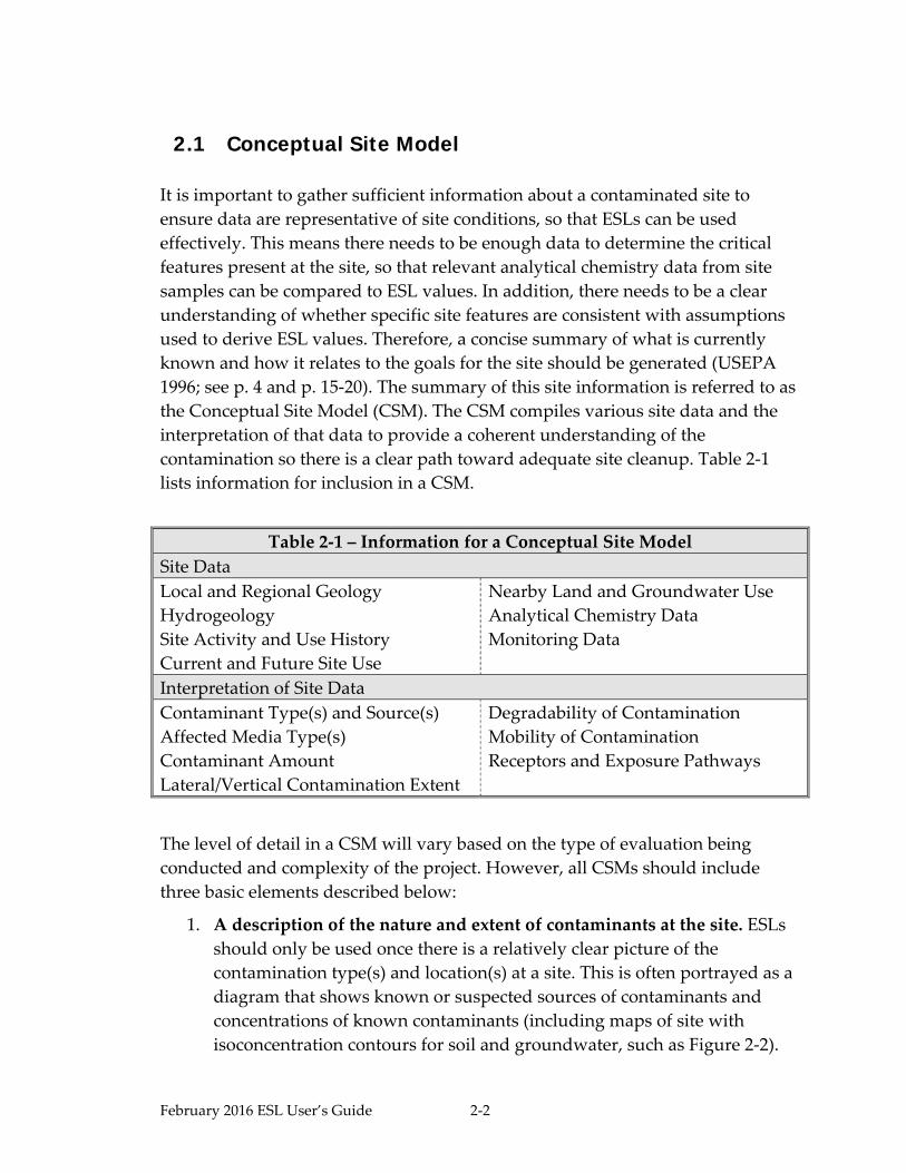
2.1 Conceptual Site Model
It is important to gather sufficient information about a contaminated site to
ensure data are representative of site conditions, so that ESLs can be used
effectively. This means there needs to be enough data to determine the critical
features present at the site, so that relevant analytical chemistry data from site
samples can be compared to ESL values. In addition, there needs to be a clear
understanding of whether specific site features are consistent with assumptions
used to derive ESL values. Therefore, a concise summary of what is currently
known and how it relates to the goals for the site should be generated (USEPA
1996; see p. 4 and p. 15‐20). The summary of this site information is referred to as
the Conceptual Site Model (CSM). The CSM compiles various site data and the
interpretation of that data to provide a coherent understanding of the
contamination so there is a clear path toward adequate site cleanup. Table 2‐1
lists information for inclusion in a CSM.
Table 2‐1 – Information for a Conceptual Site Model
Site Data
Local and Regional Geology
Hydrogeology
Site Activity and Use History
Current and Future Site Use
Nearby Land and Groundwater Use
Analytical Chemistry Data
Monitoring Data
Interpretation of Site Data
Contaminant Type(s) and Source(s)
Affected Media Type(s)
Contaminant Amount
Lateral/Vertical Contamination Extent
Degradability of Contamination
Mobility of Contamination
Receptors and Exposure Pathways
The level of detail in a CSM will vary based on the type of evaluation being
conducted and complexity of the project. However, all CSMs should include
three basic elements described below:
1. A description of the nature and extent of contaminants at the site. ESLs should only be used once there is a relatively clear picture of the
contamination type(s) and location(s) at a site. This is often portrayed as a
diagram that shows known or suspected sources of contaminants and
concentrations of known contaminants (including maps of site with
isoconcentration contours for soil and groundwater, such as Figure 2‐2).

February 2016 ESL User’s Guide 2‐3
Cross sections showing the delineation of the vertical extent of
contamination should be included (e.g., Figure 2‐3). A calculation of
residual contaminant mass in each media can also be helpful. It is also
helpful to include a summary of the site history, including operations at
the site that are known or suspected to have caused the release.
2. A description of how contaminants are moving or changing in space and time. This should address whether the extent of known
contamination is growing, migrating, or attenuating and should include a
discussion of geology and hydrogeology. For new sites, this section may
be brief, but for older and more complex sites, this section should
summarize relevant site‐specific issues such as preferential pathways
(natural and man‐made), vertical groundwater gradients, and evidence of
biodegradation. If biodegradation is occurring at a site, the degradation
byproducts should be discussed. Boring logs, well logs, maps of
subsurface utilities and other figures, as appropriate, may be used to
support this evaluation. Plots of chemical concentration versus distance or
time may be useful to illustrate contaminant migration or attenuation. If
remediation has been conducted at the site, the effectiveness of the
remediation should be evaluated.
3. An evaluation of the potential receptors and exposure pathways. This is often shown as a chart indicating which media are impacted and the
exposure pathways from each medium to potential receptors. For initial
screening at the Tier 1 level, default receptors are assumed (see Section 2.3
and Figure 2‐4). For more detailed evaluations, a site specific description
of the actual receptors – both human and environmental ‐ should be
included and the presence of sensitive receptors such as schools or day
care centers highlighted (e.g., Figure 2‐5). Exposure pathways and
receptors which may be present at the site but are not considered by the
ESLs should be noted, such as consumption of backyard produce grown
in contaminated soil or ingestion of contaminated surface water by
endangered species.


Figure 2‐4. Default Evaluation of Receptors and Exposure Pathways Used in a Tier 1 Assessment
PRIMARY SOURCES
PRIMARY RELEASE
MECHANISMSTRANSPORT
MECHANISMS EXPOSURE
MEDIA EXPOSURE
ROUTES
* The ESLs do not not include soil to indoor air screening levels. Soil gas must be sampled to evaluate this transport pathway.
Ecol
ogic
al
Rec
epto
rs
POTENTIAL RECEPTORS
SECONDARY SOURCES
Res
iden
tial
Occ
upat
iona
l
Con
stru
ctio
n &
Exc
avat
ion
Storage Tank Leaking
Surface Soils
Subsurface Soils
Groundwater
Discharge
Dermal ContactIngestion
Particulates/Volatiles Outdoor Air Inhalation
Volatilization and migration in soil
gas*Indoor Air
Outdoor Air
Inhalation
Inhalation
Dermal ContactIngestion
Dermal ContactIngestion
Leaching
Inhalation/Ingestion/Dermal Exposure
Volatilization and migration through
soil gas Indoor Air
Outdoor Air
Inhalation
Inhalation
Surface Fish/Shellfish Ingestion

Figure 2-4. Default evaluation of receptors and exposure pathways used in a Tier 1 assessment
PRIMARY
SOURCES
PRIMARY
RELEASE
MECHANISMS
TRANSPORT
MECHANISMS
EXPOSURE
MEDIA
EXPOSURE
ROUTES
* The ESLs do not model volatilization of contaminant mass in subsurface soils. Soil gas must be sampled to evaluate this transport pathway.
Eco
log
ical
Rec
ep
tors
POTENTIAL RECEPTORS
SECONDARY
SOURCES
Res
iden
tia
l
Oc
cu
pati
on
al
Co
nstr
ucti
on
& E
xc
av
ati
on
Storage Tank Leaking
Surface Soils
Subsurface Soils
Groundwater
Discharge
Dermal Contact Ingestion
Particulates/Volatiles Outdoor Air Inhalation
Volatilization and migration in soil
gas* Indoor Air
Outdoor Air
Inhalation
Inhalation
Dermal Contact Ingestion
Dermal Contact Ingestion
Leaching
Inhalation/Ingestion/Dermal Exposure
Volatilization and migration through
soil gas Indoor Air
Outdoor Air
Inhalation
Inhalation
Surface Fish/Shellfish Ingestion

February 2016 ESL User’s Guide 2‐8
2.2 ESL Workbook Content
The ESL Workbook is a Microsoft Excel file that includes multiple worksheets
that were used to calculate and summarize all the ESL for groundwater, soil,
subslab/soil gas, and indoor air. Each worksheet is color coded and appears in
the workbook in following order:
White Tabs ‐ Index of Tables
Dark Blue Tabs ‐ Summary tables showing all possible ESLs for each media type
and those selected as the Tier 1 screening value.
Red Tabs ‐ Interactive Tool that allows users to input site‐specific information
that will generate Tier 2 (T2) screening levels for a selected chemical and specific
site scenario. The tool includes separate worksheets:
o Table T2‐1: Input page for: 1) chemical selection and entry of site‐specific
information (1st yellow box); and 2) specific site contamination
concentrations (2nd yellow box). The output T2 ESLs are also given (gray
box).
o Table T2‐2: Details on which ESL were considered for the output T2 ESLs.
o Table T2‐3: Specific media and pathway concerns for the input site
contamination concentrations.
Light Blue Tabs – Calculation tables that show which parameters are used to
calculate the ESLs for Groundwater (GW):
o Table GW‐1: Direct Exposure Human Health Risk Level Calculation
o Table GW‐2: Aquatic Ecotoxicity Level Calculation
o Table GW‐3: GW Vapor Intrusion Human Health Risk Level Calculation
o Table GW‐4: Gross Contamination Level Calculation
o Table GW‐5: Taste and Odor Nuisance Level Calculation
Yellow Tabs – Calculation tables that show which parameters are used to
calculate the ESLs for Soil (S):
o Table S‐1: Direct Exposure Human Health Risk Level Calculation
o Table S‐2: Leaching to Groundwater Level Calculation
o Table S‐3: Gross Contamination Level Calculation
o Table S‐4: Odor Nuisance Level Calculation

February 2016 ESL User’s Guide 2‐9
Green Tabs – Calculation tables that show which parameters are used to
calculate the ESLs for Subslab/Soil Gas (SG):
o Table SG‐1: Vapor Intrusion Human Health Risk Level Calculation
o Table SG‐2: Vapor Intrusion Odor Nuisance Level Calculation
Purple Tabs – Calculation tables that show which parameters are used to
calculate the ESLs for Indoor Air (IA):
o Table IA‐1: Direct Exposure Human Health Risk Level Calculation
o Table IA‐2: Odor Nuisance Level Calculation
Tan Tabs ‐ Lookup Tables compiling the Input Parameters/Constants (IP):
o Table IP‐1: Physical‐Chemical Parameters
o Table IP‐2: Toxicity Values
o Table IP‐3: Direct Exposure Model Factors
o Table IP‐4: Maximum Contamination Levels (MCL) and other Drinking
water Levels
o Table IP‐5: CalEPA Ecotoxicity Aquatic Habitat Goals
o Table IP‐6: USEPA and Other Ecotoxicity Aquatic Habitat Goals
o Table IP‐7: Seafood Ingestion Risk from Bioaccumulation
2.3 Tier 1 ESLs – Default Conservative Site Scenario
Tier 1 ESL are based on conservative default Conceptual Site Model (CSM)
scenario conditions listed in Table 2‐2. This scenario is designed to protect sites
with unrestricted land and water use, shallow soil contamination, shallow
ground water, and permeable soil (see Section 2.4 for more information about
these and other specific site criteria and how they should be applied).
The Tier 1 ESL Workbook Summary Table gives screening levels for
groundwater, soil, subslab/soil gas, and indoor air. By comparing sample data to
these Tier 1 ESLs, decisions can be made regarding the need for additional site
investigation, remedial action or a more detailed risk assessment. Since a Tier 1
evaluation uses default exposure scenarios, it is most useful for screening out
sites where the concentration of a single contaminant is below its ESL for a given
medium or concentrations of a limited number of contaminants are well below
their respective ESLs. Exceedance of a Tier 1 ESL typically indicates the need for
a Tier 2 assessment.

February 2016 ESL User’s Guide 2‐10
Table 2‐2 – Tier 1 ESL Conceptual Site Model Site Scenario Criteria Tier 1 ESL Selection
Land Use Residential
Groundwater Use Drinking Water Resource
MCL Priority over Risk Based
Levels Yes
Groundwater Depth Shallow (≤ 10 ft bgs)
Soil Type for Vapor Intrusion Sand Scenario
Soil Exposure Depth Shallow (≤ 10 ft bgs)
2.4 Tier 2 ESLs – Site Specific ESL Choice and Use of Interactive Tool
Tier 2 ESL are selected by refining the default CSM to identify relevant
pathways, receptors, and concerns specific to an individual site. This is an
intermediate approach that is a relatively rapid and cost‐effective option for
preparing more quantitative site‐specific risk assessments. The following sections
give a step‐by‐step description of how to choose the correct Tier 2 ESLs for a
specific site. These steps will also help with the selection of appropriate site
specific input criteria for the ESL Workbook Interactive Tool Input Table T2‐1.
Step 1: Check ESL Applicability and Updates
Check with the overseeing regulatory agency to determine if the ESLs can be
applied to the subject site. Ensure that the most up‐to‐date version of the ESLs is
being used.

February 2016 ESL User’s Guide 2‐11
Step 2: Identify Chemicals of Potential Concern
An appropriate ESL assessment must be based on the results of adequate site
investigation.
Determine the extent of chemicals in groundwater, soil, and subslab/soil gas
and areas of potential environmental concern at the site and offsite, as
required.
Identify maximum concentrations of chemicals present in the media of
concern.
Soil data should be reported on a dry‐weight basis.
The ESLs are intended as a screening tool for sites with low levels of
contaminants, and are tabulated for one chemical and one medium (water, soil or
indoor air) only. When multiple chemicals are present or receptors are exposed
to more than one contaminated medium, the applicability of the ESLs should be carefully evaluated. If multiple contaminants are present and one or more of the
concentrations approach the respective ESLs, the cumulative risk (and hazard)
must be evaluated as described in Section 3.2.2.
Step 3: Land Use Selection
ESLs for soil, subslab/soil gas, and indoor air are selected based on the present
and anticipated future use of the site. Land uses are categorized based on the
assumed magnitude of potential human exposure (see Section 3). Two options
are available in the workbook:
Residential Land Use category is intended for sites where unrestricted future
land‐use is sought. This includes sites to be used for residences, hospitals,
day‐care centers and other sensitive purposes (DTSC 2002). ESLs listed under
this category incorporate assumptions regarding long‐term, frequent
exposure of children and adults in a residential setting. Screening levels for
residential land use are considered to be appropriate for unrestricted use of a
property.
Commercial or Industrial Use assumes that only working‐age adults will be
present at the site on a regular basis. Direct‐exposure assumptions
incorporated into the soil ESLs for commercial or industrial land use assume
shorter, less frequent exposure for receptors compared to assumptions used
for residential land use receptors (e.g., less exposure time per day). For
February 2016 ESL User’s Guide 2‐12
evaluation of commercial/industrial properties, it is recommended that site
data be compared to ESLs for both unrestricted/residential and
commercial/industrial land use.
Land use should be selected with respect to the current and foreseeable future
use of the site in question. Reference to adopted General Plan maps, zoning
maps, and local redevelopment plans is an integral part of this process.
Discussions with local planners may help identify reasonably foreseeable
changes to land use. Use of the lookup tables for sites with other land uses
should be discussed with and approved by the overseeing regulatory agency.
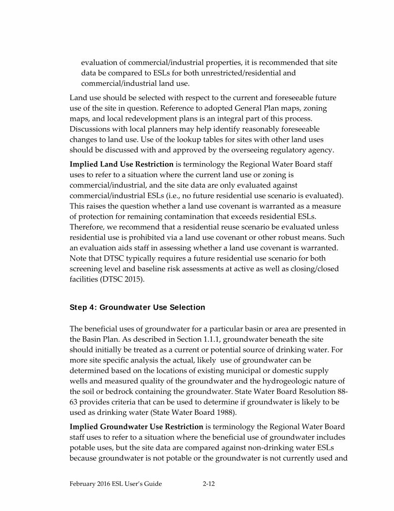
Implied Land Use Restriction is terminology the Regional Water Board staff
uses to refer to a situation where the current land use or zoning is
commercial/industrial, and the site data are only evaluated against
commercial/industrial ESLs (i.e., no future residential use scenario is evaluated).
This raises the question whether a land use covenant is warranted as a measure
of protection for remaining contamination that exceeds residential ESLs.
Therefore, we recommend that a residential reuse scenario be evaluated unless
residential use is prohibited via a land use covenant or other robust means. Such
an evaluation aids staff in assessing whether a land use covenant is warranted.
Note that DTSC typically requires a future residential use scenario for both
screening level and baseline risk assessments at active as well as closing/closed
facilities (DTSC 2015).
Step 4: Groundwater Use Selection
The beneficial uses of groundwater for a particular basin or area are presented in
the Basin Plan. As described in Section 1.1.1, groundwater beneath the site
should initially be treated as a current or potential source of drinking water. For
more site specific analysis the actual, likely use of groundwater can be
determined based on the locations of existing municipal or domestic supply
wells and measured quality of the groundwater and the hydrogeologic nature of
the soil or bedrock containing the groundwater. State Water Board Resolution 88‐
63 provides criteria that can be used to determine if groundwater is likely to be
used as drinking water (State Water Board 1988).
Implied Groundwater Use Restriction is terminology the Regional Water Board
staff uses to refer to a situation where the beneficial use of groundwater includes
potable uses, but the site data are compared against non‐drinking water ESLs
because groundwater is not potable or the groundwater is not currently used and

February 2016 ESL User’s Guide 2‐13
is unlikely to be used in the future (e.g., municipal water system). In these cases a
deed restriction may be required to ensure that groundwater will not be used in
the future. Further, because groundwater is not static, the potential for
contaminant migration needs to be considered.
Step 5: MCL Priority vs Risk-Based Screening Levels Selection
The Basin Plan directs that the lower of the primary and secondary Maximum
Contaminant Levels (MCLs) be used as an upper bound when setting cleanup
goals for groundwater designated for use as a domestic or municipal supply (see
Section 1.1). MCLs are drinking water standards adopted by the California State
Water Resources Control Board, Division of Drinking Water (DDR)1 pursuant to
the California Safe Drinking Water Act. Primary MCLs are derived from health‐
based criteria, but they also include technologic and economic considerations
based on the feasibility of achieving and monitoring for these concentrations in
drinking water. The balancing of health effects with technologic and economic
considerations may not always be appropriate for protection of the quality of all
surface water or groundwater resources.
Step 6: Groundwater Depth Selection
Depth to groundwater is an important factor in assessing the potential for vapor
intrusion resulting from contaminated groundwater. The groundwater depth
and soil type (Step 7) are used in selecting the appropriate groundwater vapor
intrusion model scenario (see Section 4.2). The selected groundwater vapor
intrusion model scenario effectively determines the amount of contaminant
attenuation (reduction in concentration) that occurs during transport from
groundwater to indoor air (GW‐IA). Groundwater depth is the primary
determinant and soil type is a secondary determinant. Depth of groundwater
should be determined from the shallowest measured depth to first groundwater
1 The California Drinking Water Program was transferred from the California Department of
Public Health in July 2014.

February 2016 ESL User’s Guide 2‐14
at a site (e.g., seasonal high water table). If groundwater is less than 10 feet bgs
(Shallow), the most conservative GW‐IA attenuation factor (Shallow Sand
Scenario; see Chapter 4) is used regardless of soil type.2 When groundwater is
10 feet bgs or more (Deep), the site‐specific soil type is employed in the selection
of the groundwater vapor intrusion scenarios, as described in Step 7.
Step 7: Soil Type Selection
The soil type is a secondary determinant in selecting the appropriate
groundwater vapor intrusion scenario (Chapter 4.2). The soil types in the vadose
should be determined based on lithological information gathered at the site
(e.g., boring logs, geotechnical testing, and cross sections). This information is
used to determine the groundwater vapor intrusion model scenario and
associated amount of contaminant attenuation that is expected to occur at a site.
Two different soil‐specific groundwater vapor intrusion scenarios were
developed for sites with deep groundwater. See the previous step for the shallow
groundwater scenario. The first scenario (Deep Sand) assumes all sand and
should be used for sites where coarse‐grained soils (sands or gravels) are
predominant. The second scenario (Fine‐Coarse) assumes a continuous, fine‐
grained soil at the water table and coarse‐grained soil beneath the building. This
scenario could also be used for sites with predominantly fine‐grained soils or
layers. Section 4.2 provides a discussion regarding the basis of these scenarios.
Step 8: Soil Exposure Depth Selection
The ESLs employ two soil contamination depth options for soil direct contact
considerations (Table 2‐3):
2 Natural (e.g., conduits created by sand lenses, fractures, or desiccation cracks), manmade
(e.g., utility lines or associated backfill) and building‐specific (e.g., below‐ground elevator
components) preferential pathways responsible for minimal attenuation of contaminant
vapors are more likely to be present and affect vapor transport in the upper 10 feet of soil.

February 2016 ESL User’s Guide 2‐15
Shallow Soil Contamination (at or above 10 feet bgs): There is potential for residents, commercial/industrial workers, and construction workers to be
exposed to contaminated soil at or above 10 feet bgs. This means that, for
most screening evaluations, two potentially exposed receptors need to be
considered: 1) residential or commercial/industrial; and 2) construction
workers.
Deep Soil Contamination (below 10 feet bgs): There is potential for construction workers to be exposed to contaminated soil below 10 feet bgs.
Regular exposure to contaminated soil at that depth by residents or
commercial/industrial workers is unlikely, unless the overlying soil were
removed, which is rare.
If chemicals are detected in shallow and deep soil, it is appropriate to evaluate
depth exposure interval.
Table 2‐3 – Soil Direct Exposure Depth Intervals
Soil Depth
Scenario:
Residential
Scenario:
Commercial/Industrial
Scenario:
Construction Worker
Land Use:
Residential
Land Use:
Commercial/Industrial
Land Use:
Any
Receptor:
Resident
Receptor:
Indoor/Outdoor
Worker
Receptor:
Construction Worker
Shallow
(≤10 feet bgs) Yes Yes Yes
Deep
(>10 feet bgs) No No Yes
Step 9: Final ESL Determination Process
The Interactive Tool uses the site‐specific scenario parameters chosen by the user
in ESL Workbook Table T2‐1, to identify the specific ESLs appropriate for each
medium. All screening levels considered for the specified contaminant are shown
in the ESL Workbook Table T2‐2. The following figures illustrate the
considerations used in the determination of the final screening level for each
medium: Figure 2‐6 (Groundwater), Figure 2‐7 (Soil), Figure 2‐8 (Subslab/Soil
Gas), and Figure 2‐9 (Indoor Air).

February 2016 ESL User’s Guide 2‐16
Figure 2‐6 – Final Site‐Specific Groundwater ESL Determination

February 2016 ESL User’s Guide 2‐17
Figure 2‐7 – Final Site‐Specific Soil ESL Determination

February 2016 ESL User’s Guide 2‐18
Figure 2‐8 – Final Site‐Specific Subslab/ Soil Gas ESL Determination
Figure 2‐9 – Final Site‐Specific Indoor Air ESL Determination

February 2016 ESL User’s Guide 2‐19
Step 10: Compare Site Data to ESLs
The maximum‐detected concentrations of a specific chemical can be input into
the Interactive Tool in ESL Workbook Table T2‐1 of the Workbook and the
specific concerns posed by those concentration levels will be identified in ESL
Workbook Table T2‐3.
Note: Initial screening typically is performed using maximum‐detected
concentrations. The use of statistical methods (e.g., 95 percent upper confidence
limit of the arithmetic mean or UCL) to estimate more site‐specific exposure
point concentrations (EPCs) and evaluate environmental risks is common for
Tier 2 and Tier 3 risk evaluations. The UCL is commonly used as the EPC for soil
where the data are averaged over the area/volume to which receptors could be
chronically exposed. Guidance for the estimation of exposure point
concentrations, use of non‐detect data, and other issues is provided in the
following documents: 1) Preliminary Endangerment Assessment Guidance
Manual (DTSC 2015), 2) Calculating Upper Confidence Limits for Exposure Point
Concentrations at Hazardous Waste Sites (USEPA 2002c), and 3) ProUCL
Version 5.0.00 User Guide and Technical Guide (USEPA 2013c). As discussed in
these documents, care should be exercised when determining the area and depth
over which the data are averaged. For soil contaminants in an anticipated
residential development, concentrations should not be averaged over an area
greater than the area of the existing or anticipated residential lot. Soil leaching to
groundwater data generally should not be averaged. For vapor intrusion
concerns, groundwater concentrations should not be averaged over an area
greater than the floor space area of existing or anticipated buildings.
Step 11: Compare Site Data to Background Levels
If information on the background concentrations of the chemicals of interest at
the site is available, compare the background concentrations to the selected ESLs.
As discussed in Section 10.2, if site‐specific background concentrations of
chemicals of concern are greater than risk‐based ESLs, the background
concentrations may be substituted. This should be pointed out in the appropriate
report. For example, arsenic concentrations in site soils typically exceed risk‐
based screening levels by one or more orders of magnitude, and there is available
information on background levels of arsenic in undifferentiated urbanized

February 2016 ESL User’s Guide 2‐20
flatland soils in the Bay Area. Thus, that value can be substituted for the risk‐
based ESL. This is further discussed in Section 10.5.3.
Step 12: Evaluate the Need for Additional Investigation, Assessment, or Remediation
Based on a comparison of available site data to the ESLs, evaluate the need for
additional action at the site. Additional actions may include additional site
investigation, preparation of a site‐specific risk assessment, source remediation,
or mitigation (to protect a threatened receptor).
Example of Interactive Tool Use: Tetrachloroethene
Tetrachloroethene (PCE) is selected as the contaminant and the specific site
scenario options are chosen from the drop down menus in the first yellow box
within the Interactive Tool ESL Workbook Table T2‐1 (Tier‐2 Site‐Specific
Inputs), as shown in Figure 2‐6. For this example site, there is soil and
groundwater data which is also entered in the second yellow box (optional step).
The final grey box shows the media specific Tier 2 ESLs for the contaminant
given the selected site scenario information. Figure 2‐7 shows the Interactive ESL
Workbook Tool Table T2‐2 (ESL Details) for this example. From this table it
becomes clear which screening levels are driving the final ESL for each media:
Groundwater: Vapor Intrusion to Indoor Air (ESL = 3 μg/L)
Soil: Leaching to Groundwater (ESL = 0.42 mg/kg)
Soil Gas: Vapor Intrusion to Indoor Air (ESL = 240 μg/m3)
Indoor Air: Direct Exposure (ESL = 0.48 μg/m3)
The site diagram shown in the Interactive Tool ESL Workbook Table T2‐3
(Specific Concerns) can be used to get a better idea of potential threats caused by
specific chemical concentrations measured at a site, shown in Figure 2‐8 for this
example. This diagram uses the concentration inputs from ESL Workbook Table
T2‐1. The final ESLs for groundwater, soil, subslab/soil gas, and indoor air are
shown within circles. Each circle is connected to boxes that show the different
ESLs considered for that media type. Red X’s will appear next to all ESLs that are
exceeded by the input site concentration data and provides a visual for specific
site consideration that could be potentially affected at this site. As seen in Figure

February 2016 ESL User’s Guide 2‐21
2‐8, the site specific concerns soil and groundwater concentrations given for this
example are:
Soil: 1) Human health risk from direct exposure to contaminated soil
2) Leaching to groundwater
Groundwater: 1) Groundwater vapor intrusion to indoor air
2) Discharge to surface aquatic habitats
Figure 2‐8 also shows that both groundwater and soil PCE concentrations at the
site are below levels where gross contamination or odor would be a concern.

February 2016 ESL User’s Guide 2‐22
Figure 2‐10 – Interactive Tool ESL Workbook Site Specific Inputs Table T2‐1 based on the example scenario described herein
Tier 2 Scenario Toggles
Contaminant: Tetrachloroethene
Land Use: Residential
Groundwater Use: Nondrinking Water Resource
MCL Priority over Risk-Based Levels: No
Shallow Groundwater
Soil Type for GW VI: Sand Scenario
Shallow Soil
Enter site data (Optional)
Soil Concentration (mg/kg) - dry weight: 5.00
Groundwater Concentration (μg/L): 100.00
Indoor Air Concentration (μg/m3):
Output Tier 2 ESLs:Soil (mg/kg): 4.2E-01
Groundwater (μg/L): 3.0E+00
Subslab/ Soil Gas (μg/m³): 2.4E+02
Indoor Air (μg/m³): 4.8E-01
Subslab/ Soil Gas Concentration (μg/m3):
Soil Depth for Direct Exposure: (Shallow ≤ 10ft bgs < Deep)
Groundwater Depth for GW VI: (Shallow ≤ 10ft bgs < Deep)
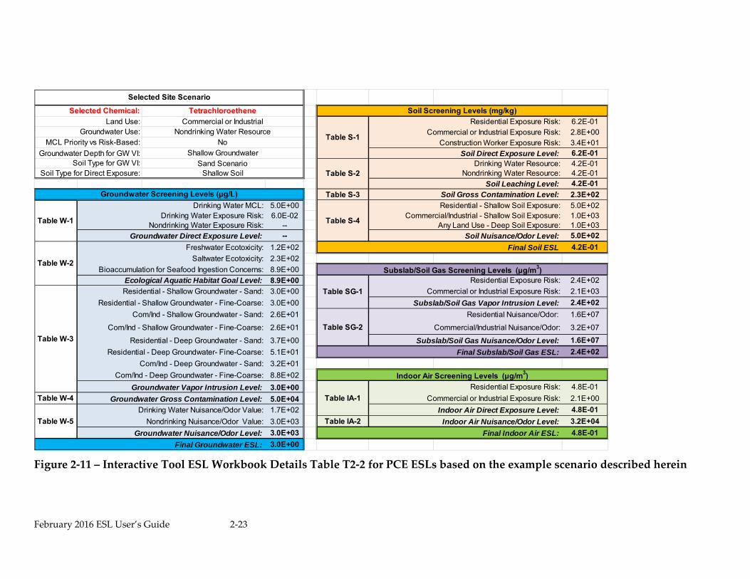
February 2016 ESL User’s Guide 2‐23
Figure 2‐11 – Interactive Tool ESL Workbook Details Table T2‐2 for PCE ESLs based on the example scenario described herein
Residential Exposure Risk: 6.2E-01Commercial or Industrial Exposure Risk: 2.8E+00
Construction Worker Exposure Risk: 3.4E+01Groundwater Depth for GW VI: Soil Direct Exposure Level: 6.2E-01
Drinking Water Resource: 4.2E-01Nondrinking Water Resource: 4.2E-01
Soil Leaching Level: 4.2E-01
Table S-3 Soil Gross Contamination Level: 2.3E+02
Drinking Water MCL: 5.0E+00 Residential - Shallow Soil Exposure: 5.0E+02Drinking Water Exposure Risk: 6.0E-02 Commercial/Industrial - Shallow Soil Exposure: 1.0E+03
Nondrinking Water Exposure Risk: -- Any Land Use - Deep Soil Exposure: 1.0E+03Groundwater Direct Exposure Level: -- Soil Nuisance/Odor Level: 5.0E+02
Freshwater Ecotoxicity: 1.2E+02 Final Soil ESL 4.2E-01
Saltwater Ecotoxicity: 2.3E+02
Bioaccumulation for Seafood Ingestion Concerns: 8.9E+00
Ecological Aquatic Habitat Goal Level: 8.9E+00 Residential Exposure Risk: 2.4E+02
Residential - Shallow Groundwater - Sand: 3.0E+00 Commercial or Industrial Exposure Risk: 2.1E+03
Residential - Shallow Groundwater - Fine-Coarse: 3.0E+00 Subslab/Soil Gas Vapor Intrusion Level: 2.4E+02
Com/Ind - Shallow Groundwater - Sand: 2.6E+01 Residential Nuisance/Odor: 1.6E+07
Com/Ind - Shallow Groundwater - Fine-Coarse: 2.6E+01 Commercial/Industrial Nuisance/Odor: 3.2E+07
Residential - Deep Groundwater - Sand: 3.7E+00 Subslab/Soil Gas Nuisance/Odor Level: 1.6E+07
Residential - Deep Groundwater- Fine-Coarse: 5.1E+01 Final Subslab/Soil Gas ESL: 2.4E+02
Com/Ind - Deep Groundwater - Sand: 3.2E+01
Com/Ind - Deep Groundwater - Fine-Coarse: 8.8E+02
Groundwater Vapor Intrusion Level: 3.0E+00 Residential Exposure Risk: 4.8E-01
Table W-4 Groundwater Gross Contamination Level: 5.0E+04 Commercial or Industrial Exposure Risk: 2.1E+00
Drinking Water Nuisance/Odor Value: 1.7E+02 Indoor Air Direct Exposure Level: 4.8E-01
Nondrinking Nuisance/Odor Value: 3.0E+03 Table IA-2 Indoor Air Nuisance/Odor Level: 3.2E+04
Groundwater Nuisance/Odor Level: 3.0E+03 Final Indoor Air ESL: 4.8E-01
Final Groundwater ESL: 3.0E+00
Table W-2
Table W-3
Selected Site Scenario
Tetrachloroethene
Commercial or IndustrialNondrinking Water Resource
No
Shallow Soil
Land Use:
Table S-4
Shallow Groundwater
Table IA-1
Table W-1
Table W-5
Indoor Air Screening Levels (μg/m3)
Table SG-2
Table SG-1
Table S-1
Table S-2
Groundwater Screening Levels (μg/L)
Selected Chemical:
Subslab/Soil Gas Screening Levels (μg/m3)
Groundwater Use:MCL Priority vs Risk-Based:
Soil Type for Direct Exposure:Soil Type for GW VI: Sand Scenario
Soil Screening Levels (mg/kg)

February 2016 ESL User’s Guide 2‐24
Figure 2‐12 – Interactive Tool ESL Workbook Specific Concerns Table T2‐3 based on the example scenario described herein
2.5 Tier 3 - Risk Assessment Derived Screening Levels
Tier 3 Screening Levels are based on alternate models and modeling input
assumptions develop by conducting a complete site risk assessments that
quantitatively evaluate the risk posed to human and/or ecological receptors by
the contaminated media. Consideration of the methodologies and potential
environmental concerns discussed in this document is still encouraged for the
development of Tier 3 screening levels. See Appendix A for other resources that
can be used during the development of Tier 3 risk‐based screening levels.

February 2016 ESL User’s Guide 3‐1
3 Methods: Direct Exposure Human Health Risk Screening Levels for All Media
3.1 Default Exposure Scenarios: Receptors and Pathways
The ESLs take into account human health risk from direct exposure to
contaminated groundwater, soil, and indoor air. The three general receptors
considered for such direct exposure are:
Residents
Both adults and children are considered residents and are the primary receptors
for a Residential Land Use site. Children often exhibit behavior such as greater
hand‐to‐mouth soil contact that can result in greater exposure to soils than those
associated with a typical adult. In addition, children have a lower body weight
relative to the predicted intake of both water and soil which results in more
conservative risk‐based concentrations for children compared to an adult‐only
assumption. Therefore, children are the primary receptors considered for
groundwater and soil ESLs for noncancer endpoints at sites with a Residential
Land Use.
Commercial or Industrial Workers
Primary receptors considered for sites with a Commercial or Industrial Land Use
are commercial/industrial workers. The commercial/industrial scenario
represents a variety of workers, from those who spend most of their workday
indoors to those who frequently work outdoors, but not workers involved in
excavation activities. A commercial/industrial worker is assumed to be an adult
who will have eight hours of exposure during the course of a work day as a full‐
time employee of a company operating on‐site. The screening levels for this
receptor are expected to protect other reasonably anticipated indoor and outdoor
workers at a commercial/industrial facility as well as visitors.

February 2016 ESL User’s Guide 3‐2
Construction Workers
Construction could occur at any site, so construction/trench workers are
considered for both Residential and Commercial Land Use scenarios. The
activities for this receptor typically involve substantial exposures to surface and
subsurface soil3 during excavation, maintenance and building construction
projects. Contact with contamination in soil via incidental ingestion, dermal
contact, and inhalation due to volatilization and fugitive dust are the main routes
of exposure. Therefore only direct contact soil ESLs consider construction/trench
worker receptors. A construction worker is assumed to be exposed to
contaminated soil during the work day for the duration of a single on‐site
construction project, lasting one year. If multiple construction projects are
anticipated, it is assumed that different workers will be employed for each
project. Even though work durations are typically of shorter due to the short‐
term nature of construction projects, chronic toxicity information was used when
developing screening levels for a construction worker receptor. This approach is
more conservative than using subchronic toxicity values since it combines
relatively short exposure duration with a chronic toxicity value.
Each receptor described above has a varying level of exposure to the different
media types through three general exposure pathways: inhalation, ingestion, and
dermal contact. Table 3‐1 shows which exposure pathways are used to calculate
the risk‐based screening levels for each media.
Table 3‐1— Exposure Pathways for Each Direct Exposure Medium
Exposure Pathway Tapwater
(Groundwater) Soil Indoor Air
Ingestion Yes Yes No
Inhalation Yes Yes Yes
Dermal Yes Yes No
3 Surface soil is considered to be 0 to 0.5 feet bgs and subsurface soil is soil beneath 0.5 feet bgs
(DTSC 2015).
February 2016 ESL User’s Guide 3‐3
3.2 Calculation of Health Risk-Based Exposure Screening Levels
The human health direct exposure ESLs for groundwater, soil, and indoor air are
calculated using standard equations taken directly from the USEPA RSLs (2015).4
These equations combine certain exposure assumptions with chemical specific
toxicity values to calculate contaminant levels with a one‐in‐a‐million (10‐6)
cancer target risk or a noncancer target hazard quotient (HQ) of 1. Since the
levels of carcinogenic or noncarcinogenic effects caused by a given chemical are
not related, both must be considered. Therefore, the final direct exposure ESL is
the lower of the cancer vs noncancer risk screening level.
3.2.1 Toxicity Values
There are four main types of toxicity values (determined using laboratory
experiments) that are used for assessing potential adverse effects to humans in
the ESL calculations:
Carcinogenic Effects
Cancer Slope Factor (SFo): Oral and dermal exposure
Inhalation Unit Risk (IUR): Inhalation exposure
Noncarcinogenic Effects
Oral Reference Dose (RfDo): Oral and dermal exposure
Reference Concentration (RfC): inhalation exposure
Input Parameters Table IP‐3 in the ESL Excel workbook shows all the toxicity
values for each chemical used to calculate the direct exposure ESLs. Since many
different laboratory experiments have been done to determine the toxicity of
each chemical, a single chemical may have several different toxicity values listed
in different reference sources. Therefore, in order to select which reference source
to use, we developed the following hierarchy for toxicity value selection.
4 The ESLs do not employ the mutagenic equations.

February 2016 ESL User’s Guide 3‐4
Toxicity Value Hierarchy Toxicity value reference sources are presented in Table 3‐2. The final toxicity
values were selected in the listed order, with the exception being that, if the
values in the CalEPA Office of Environmental Health Hazard Assessment
(OEHHA) Toxicity Criteria Database are more conservative than the Tier 1
through 3 values, then the OEHHA values are used. In general, priority is given
to toxicity values that come from publications that are peer‐reviewed, readily
available to the public, and are transparent about the methods and assumptions
used to develop the values.
Table 3‐2 – Toxicity Value Hierarchy
Tier Source
1 USEPA Integrated Risk Information System (IRIS)
2 USEPA Provisional Peer Reviewed Toxicity Values (PPRTVs)
3 Agency for Toxic Substances and Disease Registry (ATSDR)
minimal risk levels (MRLs)
4 OEHHA Toxicity Criteria Database
5 USEPA PPRTV screening toxicity values (in PPRTV appendices)
6 USEPA Health Effects Assessment Summary Table
7 Other sources (e.g., State of New Jersey cancer slope factor for
chromium VI)
Note: For instances where the toxicity values in the OEHHA Toxicity Criteria
Database are more protective than Tier 1 or 2 toxicity values, then the OEHHA
toxicity values are prioritized.
Route Extrapolation Oral to Dermal: Experiments to determine the toxicity values: SFo and RfDo are
designed to specifically test for oral exposure, however these toxicity values can
be used to derive dermal exposure toxicity values. The main difference between
oral and dermal exposure is where the chemical is absorbed, either through the
internal gastrointestinal (GI) tract or through the external skin, respectively. The
oral toxicity values only account for toxicity from the fraction of an oral chemical
dose that is absorbed through the GI tract (GIABS) and not the total exposure

February 2016 ESL User’s Guide 3‐5
amount. Therefore, oral toxicity values must first be adjusted to consider the total
exposure amount and then they can be further adjusted to account for dermal
absorption using the following factors to predict the amount of chemical (in
either contaminated soil or water) that will be dermally absorbed:
Contaminated Soil
o ABSd: Fraction of a chemical dose in soil absorbed through the skin
Contaminated Water
o FA: Fraction of a dermal chemical dose in water absorbed through
the skin
o B: Ratio of a chemical’s (in water) dermal permeability coefficients
for outer (stratum corneum) relative to inner (viable epidermis)
layers of the skin.
o Kp: Dermal permeability coefficient of a chemical in water through
the outer skin layer (stratum corneum).
o event: time a chemical in water takes to absorb through the skin
(aka lag time)
o t*: time to reach a steady state absorption rate of a chemical in
water through the skin
These absorption values are also listed in the Input Parameters Table IP‐2 in the
ESL Workbook and are used to calculate dermal exposure risk levels.
Oral to Inhalation: The oral toxicity values can also be used to derive inhalation exposure toxicity values. This method is not as universally accepted as the oral to
dermal route extrapolation, so the ESLs do not use extrapolated inhalation
toxicity values as a rule (also see the USEPA RSL Frequent Questions). One
exception is cis‐1,2‐dichloroethene which is prevalent throughout our region at
sites contaminated with chlorinated solvents.
3.2.2 Exposure Factors
The input parameters Table IP‐3 in the ESL Workbook give list all exposure
factors considered in the calculation of the ESLs. Table 3‐3 shows which specific
exposure factors are used for each media depending on the land use of a site.
Differences in exposure factors used for carcinogenic (C) vs noncarcinogenic
(NC) risk calculations are also noted in the table.

February 2016 ESL User’s Guide 3‐6
Most of the carcinogenic risk levels for the residential ESLs are calculated using
age adjusted factors that consider both child and adult exposure over a 26‐year
period typical for residential scenarios. The ESLs do not currently include
multiple age‐adjustment factors for the early years (0 – 16 years of age).
Equations that can account for multiple developmental stages can be found in
the calculations for mutagens in the RSLs.

February 2016 ESL User’s Guide 3‐1
Table 3‐3 – Exposure Factor Selection
Residential Land Use Commercial or Industrial Land Use
Tapwater
Soil
Indoor Air Tapwater
Soil
Indoor Air Shallow
Exposure
Deep
Exposure
Shallow
Exposure
Deep
Exposure
Body Weight (BW) NC: Child
C: Age Adj.
NC: Child
C: Age Adj. Adult ‐‐
NC: Child
C: Age Adj. Adult Adult ‐‐
Surface Area
(SA)
Exposed
Skin
Soil ‐‐ NC: Child
C: Age Adj.
Const.
Worker ‐‐ ‐‐
Com/Ind
Worker
Const.
Worker ‐‐
Water NC: Child
C: Age Adj. ‐‐ ‐‐ ‐‐
NC: Child
C: Age Adj. ‐‐ ‐‐ ‐‐
Soil to Skin
Adherence Factor (AF) ‐‐
NC: Child
C: Age Adj.
Const.
Worker ‐‐ ‐‐
Com/Ind
Worker
Const.
Worker ‐‐
Ingestion
Rate (IR)
Soil ‐‐ NC: Child
C: Age Adj.
Const.
Worker ‐‐ ‐‐
Com/Ind
Worker
Const.
Worker ‐‐
Water NC: Child
C: Age Adj. ‐‐ ‐‐ ‐‐
NC: Child
C: Age Adj. ‐‐ ‐‐ ‐‐
Exposure
Time (ET)
per day,
all media ‐‐ Resident Worker Resident ‐‐ Worker Worker Worker
per water
event
NC: Child
C: Age Adj. ‐‐ ‐‐ ‐‐
NC: Child
C: Age Adj. ‐‐ ‐‐ ‐‐
Exposure Frequency (EF) Resident Resident Const.
Worker Resident Resident
Com/Ind
Worker
Const.
Worker
Com/Ind
Worker
Exposure Duration (ED) NC: Child
C: Age Adj.
NC: Child
C: Age Adj.
Const.
Worker Age Adj.
NC: Child
C: Age Adj.
Com/Ind
Worker
Const.
Worker
Com/Ind
Worker

February 2016 ESL User’s Guide 3‐1
3.2.3 Equations for Health Risk-Based Screening Levels Considering a Single Chemical
Noncarcinogenic Risk-Based Goals
Ingestion Noncarcinogenic Risk-Based Goals:
Tapwater Ingestion
co
cr
cc
water
IRW RfD
1 ED EF
mg 1
μg 1000 BW
year 1
days 365 ED THQ
C
Soil Ingestion
mg
kg10IRS
RfD
1 ED EF
BW year 1
days 365 ED THQ
C6
co
cr
cc
soil
Inhalation Noncarcinogenic Risk-Based Goals:
Tapwater Vapor Inhalation
K RfC
1
hr 24
day 1 ET ED EF
mg 1
μg 1000
year 1
days 365 ED THQ
C
rcr
c
water
Soil Gas and Particulate Inhalation
PEF
1
VF
1
RfC
1
hrs 24
day 1 ET ED EF
year
days 365 ED THQ
C
rcr
c
soil
Indoor Air Inhalation
RfC
1
hr 24
day 1 ET ED EF
mg 1
μg 1000
year 1
days 365 ED THQ
C
rrr
r
air

February 2016 ESL User’s Guide 3‐2
Dermal Noncarcinogenic Risk Based Goals
Tapwater Dermal Exposure
Inorganic Chemicals
ET K L
cm 1000 DA
C wcp
3
water
Organic Chemicals
ET 6
K FA 2
L
cm 1000 DA
C , then* t ET Ifwc
p
3
waterwc
B) (1
)3B 3B (12
B 1
ET K FA
L
cm 1000 DA
C , then* t ET If
2
2wc
p
3
waterwc
Soil Dermal Exposure
mg
kg10ABSAFSA
GIABSRfD
1 ED EF
BW year
days 365 ED THQ
C6
dcsco
cr
cc
water

February 2016 ESL User’s Guide 3‐3
Carcinogenic Risk based Goals
Ingestion Carcinogenic Risk-Based Goals
Tapwater Ingestion
adjowater IFW CSF
mg 1
μg 1000
year 1
days 365 LT TR
C
Soil Ingestion
mg
kg 10 IFS CSF
year
days 365 LT TR
C6-
adjo
soil
Inhalation Carcinogenic Risk-Based Goals
Tapwater Vapor Inhalation
K IUR hr 24
day 1 ET ED EF
year 1
days 365 LT TR
C
rrr
water
Soil Gas and Particulate Inhalation
PEF
1
VF
1
mg
μg 1000 IUR
hr 24
day 1 ET ED EF
year 1
days 365 LT TR
C
rrr
soil
Indoor Air Inhalation
IUR hr 24
day 1 ET ED EF
year 1
days 365 LT TR
C
rrr
air

February 2016 ESL User’s Guide 3‐4
Dermal Carcinogenic Risk-Based Goals
Tapwater Dermal Exposure
Inorganic Chemicals
ET K L
cm 1000 DA
C wmadjp
3
water
Organic Chemicals
ET 6
K FA 2
L
cm 1000 DA
C , then* t ET Ifwmadj
p
3
waterwmadj
B) (1
)3B 3B (12
B 1
ET K FA
L
cm 1000 DA
C , then* t ET If
2
2wmadj
p
3
waterwmadj
Soil Dermal Exposure
mg
kg10ABSDFS
GIABS
CSFo
year 1
days 365 LT TR
C6
dadj
soil
Total Cancer or Noncancer Risk: All Pathways
SL Inhalation
1
SLContact Dermal
1
SL Ingestion
1
1
(SL) Level
Screening
Final

February 2016 ESL User’s Guide 3‐5
3.2.4 Cumulative Risk Considering Multiple Chemicals
Risks posed by direct exposure to multiple chemicals with similar health effects
are considered to be additive or cumulative. For example, the total risk of cancer
posed by the presence of two carcinogenic chemicals in soil is the sum of the risk
posed by each individual chemical. The same is true for chemicals that cause the
same type of noncarcinogenic health effect. Ideally, noncarcinogens are grouped
according to their mechanism of action, but more commonly they are grouped
according to target organ.
At sites where more than one contaminant is present at concentrations greater
than their respective ESLs, cumulative cancer risk and noncarcinogenic hazard
can be readily calculated as follows:
For cancer risk estimates, divide the site‐specific concentration by the ESL that is
designated as being based on a cancer endpoint (“ca” or “c”). Sum the ratios for
each chemical and multiply the total by 10‐6 (equation 15 below).
6
i
i 10 x ESL
Conc Risk
c
c
b
b
a
a
ESL
Conc
ESL
Conc
ESL
Conc
(equation 15)
For non‐cancer hazard estimates, divide the site‐specific concentration by the
ESL that is designated as based on a non‐cancer endpoint “nc” and sum the
ratios. While the individual ratio is referred to as a hazard quotient (HQ), the
cumulative ratio represents a noncarcinogenic hazard index (HI) (equation 16
below).
i
i
ESL
Conc HI
c
c
b
b
a
a
ESL
Conc
ESL
Conc
ESL
Conc
(equation 16)
A hazard index of 1 or less is generally considered to be without potential
adverse health effects. A hazard index greater than 1 suggests further evaluation
is necessary.
Additional Consideration for Assessing Cumulative Risk and Hazard
Calculating cumulative risk and hazard across pathways and media is typically
part of a Tier 3 evaluation. In particular, segregation of hazard indices by effect
and mechanism of action can be complex and time‐consuming because it is
necessary to identify all of the major effects and target organs for each chemical
and then to classify the chemicals according to target organ(s) or mechanism of

February 2016 ESL User’s Guide 3‐6
action. This analysis is not simple and should be performed under the oversight
of a toxicologist. If the segregation is not carefully done, an underestimate of true
hazard could result.
3.2.5 Groundwater Specific Exposure Considerations
Exposure pathways for groundwater are only considered in the ESLs when
groundwater is being used as tapwater for common domestic activities such as
drinking, bathing/showering, cooking, dishwashing/laundry, and flushing the
toilet. The tapwater SLs are conservative enough that most receptors should also
be protected from incidental contact with contaminated groundwater in the
environment. However, the ESLs designated for groundwater that is not a
potential source of drinking water (aka tapwater), do not consider risk from
direct water contact for any receptors. This could be a problem if recreation or
digging activities are expected to occur at a site that would expose receptors
(mostly likely construction workers or residents) to contaminated groundwater.
3.3 Other Human Health Risk Criteria
While the direct exposure soil and indoor air ESLs are solely based on the human
health risk‐based equations described above, the groundwater ESLs also take
into account other regulatory health‐based criteria (OEHHA Public Health Goals,
Division of Drinking Water Notification Levels, and Division of Drinking Water
Public Health Archived Advisory Levels for drinking water). The “Other Health‐
Based Criteria” value considered in ESL Table W‐1, is chosen according to the
hierarchy in Table 3‐4.

February 2016 ESL User’s Guide 3‐7
Table 3‐4 – Hierarchy for Other Health‐Based Criteria for Drinking Water
Tier Source
1 OEHHA Public Health Goals
2 Division of Drinking Water1 Notification Levels
3 Division of Drinking Water Public Health Archived Advisory
Levels
Note: 1 ‐ In July 2014, California’s Drinking Water Program was transferred from the
California Department of Public Health (CDPH) to the State Water Resources
Control Board’s Division of Drinking Water (DDW).
The final health risk‐based ESL for groundwater is the lower of the calculated
health risk‐based levels and the selected “other health‐based criteria level.
3.4 Exceptions
3.4.1 MCL Priority
California MCLs can be used in place of the health risk‐based levels to represent
the Basin Plan water quality objectives. MCLs are drinking water standards
adopted by the California State Water Resources Control Board, Division of
Drinking Water (DDR)5 pursuant to the California Safe Drinking Water Act.
Primary MCLs are derived from health‐based criteria, but they also include
technologic and economic considerations based on the feasibility of achieving
and monitoring for these concentrations in drinking water. The Tier 1 ESLs, (also
called MCL Priority) use the most conservative of California primary or
secondary MCLs for all chemicals with established MCLs to represent the Basin
5 The California Drinking Water Program was transferred from the California Department of
Public Health in July 2014.

February 2016 ESL User’s Guide 3‐8
Plan water quality objectives. For chemicals with no established MCL, the final
health‐risk based ESL is used.
3.4.2 Lead
The risk‐based screening levels for soil direct‐exposure to lead are 80 mg/kg for
residential land use and 320 mg/kg for commercial/industrial land use. They are
the same values used for the lead CHHSLs. These levels were calculated using a
blood lead model developed by OEHHA (OEHHA 2007) and the DTSC
LeadSpread Model (DTSC 2011a) rather than the standard USEPA algorithms. The
toxic endpoint used for the blood lead model is based on the relationship
between blood‐lead levels and cognitive ability; where an increase of 1
microgram per deciliter (μg/dL) in blood lead is calculated as having no more
than a 2.5 percent probability of decreasing intelligence quotient by more than 1
point in a child or fetus at the 90th percentile of the blood lead distribution in the
general population. The LeadSpread Model was used to estimate the concentration
in soil that would lead to a 1 μg/dL increase in blood lead for people exposed to that
soil to calculate the CHHSL for lead in soil (OEHHA 2009). The residential CHHSL
of 80 mg/kg is based on exposure to a child resident. The commercial/industrial
CHHSL of 320 mg/kg is based on exposure to a pregnant adult worker. The
evaluation of lead is discussed in HERO Human Health Risk Note 3, Issue: DTSC‐
modified Screening Levels (DTSC‐SLs) (DTSC 2016).
3.4.3 Short-Term Exposure Levels: Trichloroethene
The ESLs present screening levels for cancer and non‐cancer risks from chronic
(long term) exposure to chemicals since such levels are generally lower than
those for short‐terms exposure risks. However, for TCE, there is a new concern
for adverse effects to developing fetuses from low doses over short exposure
periods. On September 28, 2011, the USEPA Integrated Risk Information System
(IRIS) published new toxicity criteria for TCE (USEPA 2011b). The most
significant changes included a substantial reduction in the values for noncancer
inhalation toxicity factors and a change in the noncancer toxicity endpoints
(adverse effects on specific parts or functions of the human body).
Adverse noncancer health effects documented for TCE include hepatic, renal,
neurological, immunological, reproductive and developmental damage. IRIS
selected rodent studies showing adverse effects on the kidneys, the immune
system and the developing fetus for the 2011 oral reference dose (RfD). The 2011

February 2016 ESL User’s Guide 3‐9
inhalation reference concentration (RfC) is based on oral studies. The first two
endpoints (kidney and immune system) are chronic (long‐term) effects whereas
the third (fetal heart malformation) is a developmental effect, which is
necessarily the result of a short‐term exposure, in this case three weeks during
the first trimester of pregnancy. Developmental toxicity has been linked to
inhalation of TCE vapors as well as ingestion of TCE‐contaminated drinking
water with more substantial evidence for the latter.
On July 9, 2014, USEPA Region 9 issued a memorandum entitled EPA Region 9
Response Action Levels and Recommendations to Address Near‐Term Inhalation
Exposures to TCE in Air from Subsurface Vapor Intrusion (USEPA 2014d). DTSC also
has adopted the response action levels as discussed in HERO Human Health Risk
Assessment Note 5, Issue: Health‐Based Indoor Air Screening Criteria for
Trichloroethylene (TCE) (DTSC 2014). The Draft Interim Framework for Assessment of
Vapor Intrusion at TCE‐Contaminated Sites in the San Francisco Bay Region (TCE
Framework; Regional Water Board 2014) should be consulted for the integration
of these response action levels into our vapor intrusion investigation protocols.
In the TCE Framework we have also develop “Trigger Levels” for groundwater
and subslab/soil gas concentration that would trigger immediate sampling of
indoor air. In the ESL Workbook, when TCE is selected in ESL Table T2‐1, the
TCE Action Levels and Trigger Levels are shown to the right of the table in red.
These levels are also presented in Chapter 4.
The USEPA Region 9 response action levels only address the recent changes
regarding the inhalation pathway for TCE. Because fetal heart malformation risk
could increase in pregnant women exposed to TCE from contaminated drinking
water, exceedance of the noncancer, ingestion ESL for TCE in drinking water
(10 μg/L; ESL Table GW‐1), warrants more immediate action. The investigation
and cleanup of TCE‐contaminated groundwater for protection of drinking water
resources remains a priority for the Regional Water Board and groundwater
cleanup should not be delayed. When TCE is selected in ESL Table T2‐1, this
drinking water TCE Action Level is also shown to the right of the table in red.
3.4.4 Chemical Mixtures
The ESLs include health‐risk‐based screening levels for several chemical
mixtures or groups. Relevant details regarding the derivation or use of the
screening levels are presented in Chapter 9.

February 2016 ESL User’s Guide 3‐10
3.5 Site-Specific Evaluations
Site‐specific evaluations can include quantitative risk assessments (Tier 3)
evaluations, development of alternative exposure scenarios (e.g., trespasser), or
the relatively minor modification of screening levels by use of non‐default
exposure factors or fate and transport considerations. Consultation with the
overseeing regulatory agency is recommended prior to development of such
evaluations.

February 2016 ESL User’s Guide 4‐1
4 Methods: Vapor Intrusion Risk Screening Levels for Groundwater and Subslab/Soil Gas
The vapor intrusion (VI) ESLs account for potential human health risk from
direct exposure to contaminated indoor air, where the volatile contamination
originates from a subsurface source. The two general receptors considered for
such direct exposure are residents and indoor commercial/industrial workers.
The groundwater VI ESLs were developed using attenuation factors (AFs)
calculated with a hybrid model‐empirical approach. The subslab soil gas and
deeper or exterior soil gas (subslab/ soil gas) were developed using a model
approach that is a component of the Johnson and Ettinger Model (JEM; Johnson
and Ettinger 1991). These AFs are primarily intended for existing slab‐on‐grade
buildings, but can also be used for future buildings.
The VI ESLs should be used in conjunction with other VI guidance (Section 4.1.3)
and USEPA indoor air response action levels or Regional Water Board trigger
levels when dealing with trichloroethene (TCE) contamination (Section 4.3). In
addition, alternative approaches including the use of site‐specific VI models or
tracer testing to estimate site‐ or building‐specific AFs may be necessary at some
sites (Section 4.4).
4.1 Background
The field of vapor intrusion continues to shift due to continuing scientific
research, improvements in guidance, and technology advances. Several
contemporary issues are addressed by Siegel (2009) and Kram (2015).
4.1.1 Conceptual Model for Vapor Intrusion into Buildings
There are four components to the transport of contaminated subsurface soil gases
into buildings: 1) partitioning from the VOC source (groundwater or soil) into
the vapor phase; 2) primarily diffusive vapor transport in the subsurface from
the VOC source toward the building; 3) vapor entry via advection into the
building; and 4) mixing with air inside a building (indoor air). Further details are
provided in Technical Resource Document: Default Subslab Soil Gas and Soil Gas to

February 2016 ESL User’s Guide 4‐2
Indoor Air Attenuation Factors in the Environmental Screening Levels (Regional
Water Board 2016a; Appendix B).
Near source areas, the VOC vapor source can be vadose zone soil as well as
groundwater. However, away from source areas, the VOC vapor source is
typically groundwater. For a vadose zone soil VOC source, VOC vapors diffuse
upward and concentrations will be reduced (attenuated) due to the nature of
diffusion (driven by concentration gradients between the source and discharge
location such as a building crack or the atmosphere for bare soil) and subsurface
characteristics (e.g., moisture content, soil type). For a groundwater VOC source,
diffusion first occurs through the capillary fringe, which has high moisture
content and low air content. Consequently, groundwater VOC sources are
subject to much greater attenuation than vadose zone soil VOC sources,
potentially up to three orders of magnitude (McCarthy and Johnson 1993).
Furthermore, the thicker the capillary fringe, which is controlled by grain size
(fine‐grained soils such as silts and clays have thicker capillary fringes than
coarse‐grained soils such as sands and gravels), the greater the overall resistance
to vapor transport.
4.1.2 CVOC Vapor Intrusion versus Petroleum Vapor Intrusion
At most sites, chlorinated volatile organic compounds (CVOC) and petroleum
hydrocarbons are the main contaminants that pose VI threats. In contrast to
CVOCs, petroleum hydrocarbons biodegrade readily under aerobic (oxygenated)
subsurface conditions due to microorganisms normally present in soil. Aerobic
biodegradation typically reduces the contamination and limits subsurface
migration of petroleum vapors in the vadose zone. Such biodegradation has been
found to be particularly effective at UST sites such as gas stations (State Water
Board 2012a and 2012b). A discussion of the differences between CVOC and
petroleum vapor intrusion (PVI)6 is provided in Petroleum Hydrocarbons and
Chlorinated Solvents Differ in their Potential for Vapor Intrusion (USEPA 2012b). As a
6 USEPA (2015b) defines petroleum vapor intrusion (PVI) as the intrusion of vapors from
subsurface petroleum hydrocarbons and non‐petroleum hydrocarbon fuel additives into
overlying or nearby buildings and structures.

February 2016 ESL User’s Guide 4‐3
result of these differences, USEPA provides separate guidance documents for
CVOC vapor intrusion and PVI:
OSWER Technical Guide for Assessing and Mitigating the Vapor Intrusion Pathway from Subsurface Vapor Source to Indoor Air (OSWER VI Guide;
USEPA 2015a); and
Technical Guide for Addressing Petroleum Vapor Intrusion At Leaking Underground Storage Tank Sites (OUST PVI Guide; USEPA 2015b).
Since the VI ESLs do not account for biodegradation, the ESLs may be overly
conservative for petroleum‐only release sites. The UST Policy includes PVI
scenarios and screening levels for a subset of petroleum compounds.
At some petroleum release sites additional attenuation may not be occurring at a
measurable rate due to geochemical conditions and/or mass of contamination
(size of release). An analysis of the most appropriate VI approach (CVOC versus
PVI) for petroleum release sites can be necessary once there is sufficient
subsurface information to understand site conditions. The OUST PVI Guide
identifies the following types of petroleum‐contaminated sites that USEPA
considers not to be comparable to UST sites: “refineries, petrochemical plants,
terminals, aboveground storage tank farms, pipelines, and large scale fueling
and storage operations at federal facilities), or sites with releases of non‐
petroleum chemicals including comingled plumes of petroleum and chlorinated
solvents regardless of the source.” For these types of petroleum sites, USEPA
recommends addressing them using the OSWER VI Guide (USEPA 2015a;
USEPA 2015b).
4.1.3 Approaches to Evaluating Vapor Intrusion
As a consequence of the differences between CVOC VI and PVI and the potential
for unique conditions at some number of sites, there are several options to
evaluating vapor intrusion. Table 4‐1 lists these along with relevant guidance
documents.

February 2016 ESL User’s Guide 4‐4
Table 4‐1 – Vapor Intrusion Approaches
Type of
Release Regional Water Board Other Relevant Guidance
CVOC (non‐
petroleum) TCE Framework
OSWER VI Guide
DTSC VIG
Petroleum UST
or Similar
Petroleum
Release Sites
UST Policy VI Criteria
Technical Justification for Vapor
Intrusion Media‐Specific Criteria
(State Water Board 2012a)
OUST PVI Guide
Petroleum –
Large Release
Sites
TCE Framework OSWER VI Guide
DTSC VIG
4.2 Attenuation Factors for Vapor Intrusion
Vapor attenuation refers to the reduction in volatile chemical concentrations
during vapor transport from the subsurface to indoor air. The AF is a measure of
this reduction. The equation for the subslab/ soil gas AF is:
SGor SS
IASGor SS C
C AF (Equation 4‐1)
where: CIA is the mean indoor air concentration (typically μg/m3)
CSS or SG is the mean subslab or soil gas concentration (typically
μg/m3)
Therefore the AF is an inverse measurement of the concentration reduction
(attenuation) that occurs as during subsurface transport to indoor air. For
instance, an AF of 0.002 corresponds to a 500‐times reduction in concentration:
AF = 1/concentration reduction = 1/500 = 0.002. Larger AFs correspond to less
attenuation leading to greater potential for VI impacts, and smaller AFs
correspond to more attenuation with lower potential VI impacts.
The AF for groundwater to indoor air is slightly different because the
groundwater concentration unit is in μg/L. It has to be converted to a vapor
concentration (μg/m3). USEPA (2014) presents the equation as:
)m
L 1,000( H C
C AF
3GW
IAGW
(Equation 4‐2)
where: CIA is the mean indoor air concentration

February 2016 ESL User’s Guide 4‐5
CGW is the mean groundwater concentration (μg/L)
H is the dimensionless Henry’s Law Constant at a specified
groundwater temperature
L is liters
m3 is cubic meters
Conversion of the groundwater concentration to an equivalent vapor equation
assumes there is complete equilibrium between groundwater and soil gas.
Typically, this is not the case due to the capillary fringe described in Section 4.1.1.
Therefore, the use of an equilibrium groundwater concentration as a screening
level is usually conservative.
4.2.1 Development of Soil Gas Attenuation Factors
A subslab soil gas AF was derived using a model we define as the climate‐
adjusted vapor flux approach. This is essentially the vapor‐entry‐to‐building
component of the Johnson and Ettinger Model (JEM; Johnson and Ettinger 1991)
programmed using Microsoft Excel by USEPA (2004a). This subslab soil gas AF
is used to calculate a generic soil gas ESL for both subslab soil gas (subslab) and
for non‐subslab soil gas (i.e., soil gas samples collected well below the slab or
where there are no overlying structures). Table 4‐2 lists our subslab/soil gas AFs.
The background and technical justification for this model are presented in the
Technical Resource Document: Default Subslab Soil Gas and Soil Gas to Indoor Air
Attenuation Factors in the Environmental Screening Levels (Regional Water Board
2016a; Appendix B).
Table 4‐2 – Subslab and Soil Gas Attenuation Factors for Concrete Slab‐on‐
Grade Buildings
Land/Building Use Subslab and Soil Gas
Attenuation Factor Concentration Reduction
Residential 0.002 500
Commercial/Industrial 0.001 1,000
Note: For other building foundations (e.g., basements), the overseeing regulatory
agency should be consulted. For buildings with crawl spaces, the Regional Water Board
employs an AF of 1.0 as discussed in the TCE Framework (Regional Water Board 2014).
February 2016 ESL User’s Guide 4‐6
4.2.2 Development of Groundwater Attenuation Factors
Derivation of the groundwater AF consisted of:
1. Development of appropriate scenarios based on depth to groundwater
and soil layer design; and
2. Calculation of chemical‐specific groundwater AF using the appropriate
version of the JEM.
The model versions used include the one‐layer or screening version of the
groundwater JEM (GW‐SCR) modified by DTSC‐HERO (2014), and the three‐
layer or advanced version of the groundwater JEM (GW‐ADV; USEPA 2004a).
The latter has been updated to be consistent with ESL toxicity values and the
physical and chemical constants that DTSC‐HERO adapted from the USEPA
RSLs in the GW‐SCR model. Appendix C includes a copy of model runs for PCE
and a table of input parameters for each groundwater VI scenario in Table 4‐3 for
both a residential building and a commercial/industrial building.

February 2016 ESL User’s Guide 4‐7
Table 4‐3 – Groundwater Vapor Intrusion Scenarios for Existing Residential
and Commercial/Industrial Buildings
Depth to Groundwater
(feet bgs)
Coarse‐Grained Soil
(sand or gravel)
Fine‐Grained Soil
(silt or clay)
Shallow
(≤10 feet bgs) Shallow Sand Scenario1
Deep
(>10 feet bgs) Deep Sand Scenario2 Fine‐Coarse Scenario3
Notes: 1 – Shallow Sand Scenario (GW‐SCR JEM) – Use if first groundwater is shallow (≤10
feet bgs) and predominantly coarse‐grained soils or if high likelihood of
preferential pathways (manmade or natural). This scenario is the default Tier 1
scenario.
2 – Deep Sand Scenario (GW‐SCR JEM) – Use if first groundwater is deep (>10 feet
bgs) and predominantly coarse‐grained soils and lower likelihood of preferential
pathways.
3 – Fine‐Coarse Scenario (GW‐ADV JEM) – Use if first groundwater is deep (10 feet bgs) and there is a continuous fine‐grained soil layer(s) at the water table with a low
likelihood of preferential pathways. This scenario can also be used for sites with
predominantly fine‐grained soils or layers if consistent with the CSM. This scenario
was developed using a hybrid model/empirical approach described in the text.
The Sand Scenarios (shallow and deep groundwater) are applied in cases of
predominantly coarse soils or where the likelihood of manmade or natural
preferential pathways is high. The Sand Scenario screening levels are developed
using the JEM (DTSC‐HERO December 2014 GW‐SCR version) with sand as the
only soil type and a 5‐foot depth to groundwater (shallow) or 10‐foot depth to
groundwater (deep). Regional Water Board staff considers that preferential

February 2016 ESL User’s Guide 4‐8
pathways7 responsible for minimal attenuation of contaminant vapors are more
likely to be present and affect vapor transport in the upper 10 feet of soil. As the
user will observe, the additional 5 feet of sand in the Deep Sand scenario does
not provide much additional attenuation.
The Fine‐Coarse Scenario is appropriate if groundwater is deep (10 feet bgs) and there is a continuous fine‐grained soil layer(s)8 at the water table with a low
likelihood of preferential pathways. This scenario can also be used for sites with
predominantly fine‐grained soils or layers if consistent with the CSM. This
scenario was developed using a hybrid model‐empirical approach between 1999
and 2005. The process of developing the fine‐coarse scenario was iterative over
several years. This process involved the identification of input parameters
sufficiently representative of the general site conditions found in the San
Francisco Bay region while also resulting in calculated values that are consistent
with empirical data collected from sites in the region.
4.2.3 Site-Specific Attenuation Factors for Vapor Intrusion
Site‐specific vapor intrusion models are typically used to evaluate the potential
for site conditions to have greater attenuation (smaller AFs) than provided by
using the ESLs. These models can be used for sites with existing or future
buildings. The model most commonly used is the JEM. Regional Water Board
staff developed recommendations for use of the JEM to ensure consistency and
facilitate review of modeling reports. The recommendations are included in
Appendix D. The TCE Framework discusses how Regional Water Board staff
evaluates and weighs the results of models in the multiple lines of evidence
approach.
7 Preferential pathway types include: natural (conduits created by sand lenses, fractures, or
desiccation cracks), manmade (utility lines or associated backfill), or building‐specific (below‐
ground features or significant openings).
8 The presence of a continuous fine‐grained layer (e.g., wet clay) can act as a significant barrier
to vertical vapor migration, but the effect dissipates quickly at distances close to the clay
layer’s termination point (Bozkurt et al. 2009).

February 2016 ESL User’s Guide 4‐9
Alternatives to models include tracer testing to derive building‐specific AFs and
site‐specific AFs developed from empirical data (McHugh et al. 2004; McHugh et
al. 2007; McHugh et al. 2008; King et al. 2010; DTSC 2011; USEPA 2015). As
discussed in the Technical Resource Document: Default Subslab Soil Gas and Soil Gas
to Indoor Air Attenuation Factors in the Environmental Screening Levels ( Regional
Water Board 2016a; Appendix B), Regional Water Board does not accept
building‐specific attenuation factors based on a single pair of subslab and indoor
air samples due to the spatial variability previously discussed. Rather, per
McHugh et al. (2007), all data should be used to develop a single attenuation
factor for a building.
4.3 TCE Vapor Intrusion Trigger Levels for Indoor Air Sampling
As discussed in Chapter 3, USEPA Region 9 developed ARALs and URALs,
which are TCE indoor air response action levels for both residential and
commercial exposure scenarios intended to protect women of reproductive age.
In the TCE Framework, the Regional Water Board calculated concentrations for
TCE in soil gas and groundwater to prioritize indoor air sampling due to
concerns regarding potential TCE short‐term effects. These values do not
supplant the appropriate ESLs for evaluating the potential for chronic effects.
Rather they are a prioritization tool for indoor air sampling. Most VI site
investigations follow the stepwise approach, starting with the collection of soil,
soil gas and groundwater data and then moving towards subslab soil gas and
indoor air sampling later in the process. The Trigger Levels are intended to
prioritize indoor air sampling when the potential threat level may be high
enough to exceed the ARALs. The Trigger Levels are based on the noncancer
hazard; that is, the target concentrations are the indoor air ARALs (2 μg/m3 and 8
μg/m3 for residential and commercial/ industrial exposure scenarios,
respectively). The USEPA response action levels and Regional Water Board
Trigger Levels are listed on Table 4‐4.

February 2016 ESL User’s Guide 4‐10
Table 4‐4 – TCE ESLs, Action Levels for Indoor Air (Response), and Groundwater and
Soil Gas Trigger Levels (Sample Indoor Air)
Medium
Residential Commercial/Industrial
Cancer Risk
ESL
Noncancer
Hazard ESL Lowest ESL
Trigger and
Action
Levels
Cancer Risk
ESL
Noncancer
Hazard ESL Lowest ESL
Trigger and
Action
Levels
Indoor Air (IA)
(μg/m3) 0.68 2.1 0.68
2.0
Accelerated
Response1 3.0 8.8 3.0
8.0
Urgent
Response1
Subslab/ Soil Gas*
(μg/m3) 300 1,100 300
1,000
Sample IA 3,000 8,800 3,000
8,000
Sample IA
Shallow GW
(μg/L)
Sand Scenario2
5.6 17 5.6 17
Sample IA 49 140 49 140
Sample IA
Deep GW (μg/L)
Sand Scenario3 6.9 21 6.9
21
Sample IA 60 180 60
180
Sample IA
Deep GW (μg/L)
Fine‐Coarse
Scenario4
170 520 170 520
Sample IA 1,500 4,400 1,500 4,400
Sample IA
Notes: 1 – Response Action Levels – The Accelerated Response Action Levels (ARALs) and Urgent Response Action Levels (URALs) are
USEPA‐specified concentrations in indoor air that prompt immediate response actions to reduce exposure (for information on
response actions and timing of responses see the Interim Framework for Assessment of Vapor Intrusion at TCE‐Contaminated Sites
in the San Francisco Bay Region; Regional Water Board October 2014).
2 – Shallow Sand Scenario – Use if first groundwater is shallow (≤10 feet bgs) and predominantly coarse‐grained soils or if high
likelihood of preferential pathways (manmade or natural). This scenario is the default Tier 1 scenario.
3 – Deep Sand Scenario – Use if first groundwater is deep (>10 feet bgs) and predominantly coarse‐grained soils and lower likelihood of
preferential pathways.
4 – Fine‐Coarse Scenario – Use if first groundwater is deep (10 feet bgs) and there is a continuous fine‐grained soil layer(s) at the water
table with a low likelihood of preferential pathways. This scenario can also be used for sites with predominantly fine‐grained soils
or layers if consistent with the CSM.
* – ESLs and Trigger Levels for soil gas vary slightly due to different exposure factors with the USEPA ARALs/URALs and the ESLs.

February 2016 ESL User’s Guide
5-1
5 Methods: Ecotoxicity Aquatic Habitat Screening Levels for Groundwater
The default conceptual site model for the Tier 1 ESLs assumes that groundwater
could discharge into a body of surface water and impact aquatic habitats; either
through downgradient migration of groundwater through porous soils or due
preferential pathways (e.g., discharge via a storm drain). Therefore groundwater
ecological toxicity screening levels are based on criteria for surface water
receptors and bioaccumulation toxicity data for human ingestion of seafood from
contaminated surface water habitats. The implied point of compliance is near the
edge of the surface water body where chemicals in groundwater begin to
discharge or intermix with surface water. This approach does not consider
dilution or attenuation of groundwater upon discharge to surface water because
benthic organisms may be exposed to the full concentration of chemicals in
groundwater prior to mixing with surface water.
The criteria are presented in ESL Tables IP‐5 (California levels), IP‐6 (USEPA
levels) and IP‐7 (California Toxics Rule seafood ingestion bioaccumulation
levels). The lower of the seafood ingestion ESL and the freshwater and saltwater
aquatic receptor toxicity ESLs (described below) is used as the final ecological
aquatic habitat ESL.
5.1 Aquatic Receptor Toxicity Criteria
Toxicity criteria for both freshwater and saltwater receptors are considered for
the final ecological aquatic habitat ESL. The lower of the two screening levels
should be used when the habitat is influenced by both freshwater and saltwater
sources, as is the case for estuarine habitats found in the San Francisco Bay Area.
The primary sources of data for surface water toxicity criteria, specific to
California, listed in ESL Table IP‐5 are:
the Basin Plan (Regional Water Board 2013);
the California Toxics Rule (USEPA 2000); and,
A Compilation of Water Quality Goals (State Water Board 2015).
Other sources listed in ESL Table IP‐6 include the following:
USEPA Ecotox Thresholds (USEPA 1996a);
USEPA National Recommended Water Quality Criteria (USEPA 2002a);

February 2016 ESL User’s Guide
5-2
U.S. Department of Energy (USDOE) Preliminary Remediation Goals for
Ecological Endpoints (USDOE 1997); and,
Ontario Ministry of Environment and Energy (MOEE) Rationale for the
Development and Application of Generic Soil, Groundwater and Sediment
Criteria (MOEE 1996).
For each chemical, a final chronic and acute toxicity level for both freshwater and
saltwater receptors is selected in the workbook calculation ESL Table GW‐2. The
chronic level is the lower of the Basin Plan objective versus a “Chronic Goal”
level which is selected using the hierarchy, shown in Table 5‐1. If no chronic level
is available, 10% of an acute level is used instead.
Table 5‐1 – Aquatic Receptor Toxicity Value Hierarchy
Tier Chronic Source
1 CTR CCC
2 USEPA CCC
3
Lowest of: a) USEPA AWQC; b) FCV Threshold Value (or the Tier II
value cited in the Ecotox Thresholds if no AWQC or FCV); or 3) 50
percent USEPA Chronic LOEL
4 USDOE Chronic PRG
5 50 percent MOEE Chronic AWQC or LOEL
Tier Acute Source
1 CTR CMC
2 USEPA CMC (or Acute LOEL if no CMC)
3 Other aquatic water quality criteria (LC50)
Abbreviations: AWQC – USEPA Ambient water quality criteria
CCC – Criterion Continuous Concentration
CMC – Criterion maximum concentration
CTR – California Toxics Rule (USEPA 2000)
Ecotox – USEPA Ecotox Thresholds (USEPA 1996a)
FCV – Final chronic value
LC50 – Lethal concentration that kills 50% of the population.
LOEL – Low observed effects level
USDOE – US Department of Energy
PRG – USDOE Preliminary Remediation Goal (USDOE 1997)
MOEE – Ontario Ministry of Environment and Energy

February 2016 ESL User’s Guide
5-3
5.2 Exceptions
Barium – The USEPA Ecotox goal for barium (3.9 μg/L; USEPA 1996a) was
excluded as a screening level in ESL Table IP‐6 and not included in the
lookup table for groundwater due to low confidence in the goal.
Chemical‐specific USDOE Preliminary Remediation Goals (USDOE 1997)
are used in place of USEPA chronic LOELs when the LOEL was
developed for a general group of compounds rather than a specific
chemical.
Selenium – The surface water goals for selenium in ESL Table IP‐6 are
from the California Toxics Rule as promulgated in 40 Code of Federal
Regulations Part 131: Water Quality Standards, Establishment of Numerical
Criteria for Priority Toxic Pollutants for the State of California (USEPA 2000).
However, goals for selenium are based on total recoverable, rather than
dissolved, concentrations
5.3 Site-Specific Evaluations
For sites where groundwater concentrations exceed the ecological aquatic habitat
ESLs, site‐specific evaluations for groundwater discharge to surface water and
impact to aquatic habitats can be performed. In general a multiple lines‐of‐
evidence approach becomes necessary the closer the site is to a surface water
body and becomes increasingly subject to surface water influence. Similarly,
proximity to surface water can necessitate implementation of near‐shore
hydrogeologic investigations. Options for site‐specific evaluations include:
Evaluation of background concentrations of metals in groundwater –
Background concentrations of barium, boron, copper, lead, mercury,
selenium, thallium, and zinc have been reported in excess of the
groundwater aquatic habitat ESLs in the Bay Area and may be excluded
from further consideration depending on site‐specific conditions.
Fate and transport modeling (e.g., development of dilution‐attenuation
factors).
Site‐specific, chronic aquatic toxicity testing using appropriate species,
lethal and sublethal endpoints, and contaminated site groundwater.
Similar to the Regional Water Board’s National Pollutant Discharge
Elimination System (NPDES) permits, it may be considered important to

February 2016 ESL User’s Guide
5-4
include a sensitive species (e.g., Americamysis bahia) in the testing program.
In addition, consideration should be given to testing of the early life stage
as well as the full life‐cycle.
Near‐shoreline hydrogeologic investigations – These typically are
performed in conjunction with modeling (validation) and consist of
identifying groundwater discharge zones, sampling or monitoring
groundwater/sediment porewater in those zones, and estimating mass
discharge (Chadwick and Hawkins 2008, Washington Department of
Ecology 2009). The default point of compliance for groundwater is the
area outside the influence of the water body (i.e., where the chemistry
reflects contaminated groundwater rather than surface water). These
investigations can also be targeted to understand the presence of the
hyporheic zone and its attenuation potential (Landmeyer et al. 2010).
The hyporheic zone, where present, is the saturated sediment zone beneath and
adjacent to a surface water body where the surface water readily exchanges. It’s
an important area of biogeochemical cycling of nutrients, and provides habitat
and refugia for a range of organisms. Landmeyer et al. (2010) studied the
attenuation (concentration reduction) of oxygenates in four different hyporheic
zones and found that attenuation was primarily the result of physical processes
such as dilution and dispersion. There was a small contribution in attenuation by
biodegradation. While some contaminant degradation may be enhanced within
this zone, there is also potential for contaminant accumulation due to organic‐
rich sediments resulting in toxicity to benthic organisms, which form the base of
the food chain. The hyporheic zone can be damaged by the construction of
shoreline improvements (e.g., seawalls) or filling (Environment Agency 2009). It
is not appropriate to assume contaminant degradation will occur to a sufficient
degree within the hyporheic zone to avoid benthic organism toxicity and
contaminant discharge without site‐specific evidence.

February 2016 ESL User’s Guide 6-1
6 Methods: Leaching to Groundwater Screening Levels for Soil
Soil screening levels for protection of groundwater are intended to address
potential leaching of chemicals from vadose‐zone soils and subsequent migration
to groundwater. The soil screening levels are back‐calculated based on target
groundwater screening levels for each groundwater use:
Drinking Water: Tier 1 Groundwater ESLs
Nondrinking Water: Lowest of the ecological aquatic habitat screening
level, gross contamination water screening level, groundwater vapor
intrusion screening level and non‐drinking water odor nuisance screening
level.
The groundwater vapor intrusion screening level input for ESL Table S‐2 is
selected solely from the default shallow groundwater/any soil type residential
scenario. For the deep groundwater with fine‐coarse soil type or different land
use, a manual calculation of the Soil Leaching to Groundwater ESL would be
necessary. Instructions for the manual calculation are included in Appendix B.
Leaching‐based screening levels were generated only for chemicals considered to
be significantly soluble and mobile in groundwater under normal, ambient
conditions (pH 5.0 to 9.0 and normal redox conditions). Leaching‐based soil
screening levels were not developed for metals. Leaching of metals from soil is
highly dependent on the species of the metal present and the geochemical nature
of the soil. At sites where physical‐chemical conditions may promote enhanced
leaching of metals and other chemicals from soils or waste piles, the use of
laboratory‐based leaching tests is recommended.
6.1 Calculation of Soil Leaching Screening Levels
Computer applications, SESOIL and AT123D, were combined to develop an
algorithm (eq. 9a) to model leaching of chemicals from the vadose zone and
subsequent migration of the leachate to groundwater, respectively. This
algorithm was originally developed by the state of Oregon (Anderson 1992),
slightly modified for use by the Massachusetts DEP (MADEP 1994) and then
incorporated into the MOEE lookup table guidance (MOEE 1996).

February 2016 ESL User’s Guide 6-2
Csoil = DAF x Cgw x 0.001 mg/μg (equation 9a)
DAF = (6207 x H) + (0.166 x Koc) (equation 9b)
where:
Csoil = leaching based soil concentration (mg/kg);
DAF = SESOIL‐based dilution‐attenuation factor;
Cgw = target groundwater screening level (μg/L).
H = Henryʹs Law Constant (atm‐m3/mol);
Koc = organic carbon partition coefficient (cm3/g);
The final soil leaching screening levels were calculated using the above empirical
equation. However, for highly sorptive chemicals the screening levels were set to
the chemicals’ theoretical soil saturation. Highly sorptive chemicals are identified
if both of the following chemical specific criteria are true:
Calculated Csoil > 0.001
Koc > 30,000 cm3/g
The Koc threshold of 30,000 cm3/g for designating chemicals as highly sorptive is
based on modeling carried out by the Hawaiʹi Department of Health (HDOH
1995). HDOH used the SESOIL model with input values for annual rainfall (400
cm/year or 158 inches/year), infiltration rate (144 cm/year or 57 inches/year), and
permeable soil overlying fractured bedrock. These input values are much larger
than are expected in California, and therefore use of this threshold Koc value for
determination of highly sorptive chemicals in California is conservative.
6.1.1 Specific Model Calculation Inputs
SESOIL models the generation and downward migration of leachate in the
vadose zone. The AT123D application models the mixing of leachate with
groundwater immediately below the contaminated area. A more detailed
discussion of the derivation and application of the SESOIL/AT123D algorithm as
modified by the Massachusetts DEP and adopted for use by the MOEE is
provided in MOEE (1996) and MADEP (1994). The algorithm is based on a three‐
meter thick vadose zone characterized by one meter of contaminated soil
between two one‐meter thick layers of clean soil (Table 6‐1). The lower layer
immediately overlies groundwater. All vadose‐zone soil is conservatively
assumed to be very permeable sand that freely allows the migration of leachate
to groundwater. The organic carbon content of the soil is assumed to be

February 2016 ESL User’s Guide 6-3
0.1 percent. Mixing with groundwater is modeled over a 10‐meter by 10‐meter
area. Use of a thicker sequence of contaminated soil would not significantly alter
the results of the model given the assumed 1‐meter depth to groundwater.
Table 6‐1 – Soil Leaching to Groundwater Model Design
Soil Depth Modeled Soil Type
0 to 1 meter bgs Clean Sand
1 to 2 meters bgs Contaminated Sand
2 to 3 meters bgs Clean Sand
3 meters bgs Water Table
Annual rainfall is assumed to be 1,100 mm (approximately 43 inches). A total of
720 mm (28 inches) of the total rainfall is assumed to infiltrate the ground surface
and reach groundwater (conservative for most portions of the San Francisco Bay
Area where a Mediterranean climate is prevalent). Biodegradation during
migration of leachate to groundwater is not considered. The model does allow
for resorption and re‐volatilization of chemicals from the leachate during
migration based on the physical‐chemical properties of the chemical and the
assumed soil properties. Groundwater is assumed to flow at a moderate rate of
approximately 73 meters (240 feet) per year. The concentration of a chemical in
leachate is assumed to be further reduced upon mixing of the leachate with
groundwater using a dilution factor of approximately 3.
For moderately volatile and sorptive chemicals, screening levels developed using
the SESOIL‐derived algorithm are similar to screening levels generated using the
full SESOIL application under a scenario where contaminated soil is within a few
meters of groundwater (HDOH 1995). Comparison to screening levels developed
using SESOIL suggests that the simplified algorithm may be conservative in the
following cases:
Leaching of highly volatile chemicals;
Leaching of highly sorptive chemicals;
Leaching of highly biodegradable chemicals;
Sites where the depth to groundwater is greater than 10 meters below the
bottom of the contaminated soil.

February 2016 ESL User’s Guide 6-4
As the distance between the base of contaminated soil and groundwater
increases, there is additional time and area for chemicals to volatilize out of the
leachate, resorb to soil particles or degrade by naturally occurring biological
processes. Site‐specific evaluation of the potential for leaching of chemicals from
soil may be warranted in such cases (including more rigorous modeling,
laboratory leaching tests, and groundwater monitoring).
Although these soil leaching screening levels could be applied to saturated soil,
there should be a reasoned analysis of potential limitations. For instance,
laboratory analysis of soil samples collected beneath the water table will detect
both contaminants sorbed to the soil matrix as well as dissolved in groundwater.
Away from source areas, saturated zone soil samples may be detecting the
groundwater plume. Application of these screening levels to that situation may
not be helpful.
6.2 Exceptions
6.2.1 Pentachlorophenol and Bis(2-ethylhexyl)phthalate
Pentachlorophenol and bis(2‐ethylhexyl)phthalate (aka di(2‐ethylhexyl)
phthalate or DEHP) are significantly more soluble than other highly sorptive
chemicals. Leaching‐based screening levels for these chemicals were developed
using only the SESOIL algorithm described above.
6.2.2 Polychlorinated Biphenyls (PCBs)
Based on our experience, the majority of PCB mixture releases identified in the
Bay Area have been Aroclor mixtures 1242, 1254, or 1260. The default Koc of
33,000 cm3/g presented in ESL Table S‐2 was considered to be adequately
conservative for this range and used in the leaching model. For less chlorinated
PCB mixtures, a site‐specific evaluation of potential leaching concerns and
possible vapor emission concerns is required.
6.2.3 Perchlorate
A leaching‐based soil screening level was developed for perchlorate (ClO4‐).
Perchlorate is a salt, and is not sorptive, volatile or biodegradable under normal
conditions. Use of the SESOIL/AT123D algorithm was therefore not considered

February 2016 ESL User’s Guide 6-5
appropriate. As an alternative, the simple, chemical partitioning model presented
in the USEPA Soil Screening Level Guidance document (USEPA 1996b) was
used:
DAF
ρ
H'θθfKCC
b
awococwatersoil
(Equation 10a)
where:
Csoil = soil screening level for leaching concerns (mg/kg);
Cwater = target dissolved‐phase concentration of chemical (mg/L);
Koc = sorption coefficient;
foc = fraction organic carbon in soil;
θw = water‐filled porosity;
θa = air‐filled porosity;
Hʹ = dimensionless Henryʹs Law constant;
ρb = soil bulk density (g/cm3);
DAF = dilution/attenuation Factor
This model can be used to back‐calculate the total soil concentration of a
chemical based on a target dissolved‐phase concentration of the chemical in the
soil (i.e., concentration in leachate). For perchlorate, Koc and Hʹ are presumed to
be zero and the equation reduces to:
DAFρ
θCC
b
wwatersoil
(Equation 10b)
The default water‐filled porosity in the models is 0.15 and the default soil bulk
density is 1.5.
6.3 Site-Specific Evaluations
For sites where groundwater is relatively shallow, the most direct approach to
evaluating soil leaching to groundwater is to conduct a groundwater
investigation. However, if the depth to groundwater is deep, site‐specific
evaluations might include fate and transport modeling and/or simulated
leaching tests performed in a laboratory.
Site‐specific evaluations of soil contaminant leachability can include
groundwater sampling or column leaching tests.

February 2016 ESL User’s Guide 6-6
For instance, DAFs that address mixing of contaminants leached from soil with
groundwater can be calculated using equations provided in the USEPA Soil
Screening Guidance: Technical Background Document (USEPA 1996b) or other
sources. For the Bay Area, simple leachate/groundwater mixing DAFs for
shallow aquifers would typically fall in the range of 5 for silty soils to 20 for
sandy soils, assuming a 2 meter thick shallow aquifer, 30 percent effective
porosity, infiltration rate of 8 centimeters per year (3 inches/year or
approximately 15 percent of total, average rainfall), and hydraulic conductivities
of 2 meters per day and 15 meters per day, respectively. Potentially less
conservative DAFs that also address adsorption, volatilization and other factors
can be calculated using more rigorous models (e.g., SESOIL). Consultation with
the overseeing regulatory is recommended before implementing such an
evaluation.
For laboratory leaching tests, the more common approaches include the
Synthetic Precipitation Leachate Procedure (USEPA Method 1312) or the
California Waste Extraction Test modified with an alternative extractant such as
deionized water, rainwater (pH adjusted and buffered), or groundwater.

February 2016 ESL User’s Guide 7-1
7 Methods: Gross Contamination Screening Levels for Groundwater and Soil
Gross contamination screening levels are intended to restrict the presence of
potential non‐aqueous phase liquid (NAPL; aka “free product”) and limit the
overall degradation of both groundwater and soil quality.
7.1 Media Specific Gross Contamination Approach
The gross contamination screening levels were determined for each media as
follows:
Groundwater: one‐half the solubility of a chemical and a maximum of
50,000 μg/L for any chemical based on general resource degradation
concerns (ESL Table GW‐4, after MADEP 1994).
Soil: The theoretical saturation level of a chemical in soil (Csat; ESL Table
S‐3) is used as the gross contamination soil ESL, except for the TPH
mixtures (see below). Csat corresponds to the contaminant concentration in
soil at which the absorptive limits of the soil particles, the solubility limits
of the soil pore water, and saturation of soil pore air have been reached
(USEPA 1996). Above this concentration, the soil contaminant may be
present as NAPL. The primary intent of Csat is for calculating the
volatilization factor employed in the algorithm for inhalation of volatiles
exposure pathway for soil direct contact screening levels. At Csat, the
emission flux from soil to air for a chemical reaches a plateau. Volatile
emissions will not increase above this level no matter how much more
chemical is added to the soil.
7.2 Exception: Total Petroleum Hydrocarbon Mixtures
Our values for TPH‐mixture solubility are based on Shiu et al. (1990). The value
for TPH‐diesel is used as a surrogate for TPH‐Stoddard solvent.
For complex mixtures of chemicals such as TPH, Csat significantly underestimates
the concentration where there is mobile or migrating NAPL because it does not
consider effective solubility or vapor pressure (Brost and DeVaull 2000). For TPH

February 2016 ESL User’s Guide 7-2
mixtures in soil, residual saturation (Sr) is more useful as a gross contamination
screening level because it represents the concentration above which NAPL in soil
may be mobile or migrating (i.e., free product).
In and near the actual release locations (i.e., source areas), some proportion of
migrating or mobile NAPL (free product) becomes adsorbed in soil pores
through which it travels. This is referred to as residual NAPL, and it is bound and immobile in soil because of capillary forces. It also can be referred to as
discontinuous NAPL (USEPA 1995). Eventually, after the leak or release has
stopped, the migrating or mobile NAPL becomes depleted and what remains is
relatively immobile residual NAPL held by capillary tension in soil pore spaces.
Residual NAPL in soil poses a risk in its immediate vicinity (USEPA 1999), and it
can sustain groundwater plumes through dissolution and vapor plumes through
volatilization.
Residual saturation is dependent on many factors related to the characteristics of
the mixture (e.g., viscosity, density) and soils (e.g., pore sizes) (USEPA 1995). In
finer‐grained soils, residual saturation is higher because there is greater surface
area for capillary forces to hold NAPL in place. Brost and DeVaull (2000) provide
a discussion of residual saturation and provide values for TPH gasoline, TPH
diesel, and TPH motor oil based on a range of soil textures. For the gross
contamination soil ESLs for TPH mixtures, the lowest (most conservative) values
of Sr are used: 1,000 mg/kg (TPH gasoline); 2,300 mg/kg (TPH Stoddard solvent
and TPH diesel; note the TPH diesel value is used as a surrogate for TPH
Stoddard solvent); and 5,100 mg/kg (TPH motor oil). Site‐specific evaluations of
residual saturation can be conducted (USEPA 1996).

February 2016 ESL User’s Guide 8-1
8 Methods: Taste and Odor Nuisance Screening Levels for All Media
8.1 Groundwater Taste and Odor Nuisance Levels
The Basin Plan defines the beneficial uses of municipal and domestic water
supply to include protection against unpleasant odors and tastes.
8.1.1 Groundwater: Drinking Water Resource
ESL Table GW‐5 presents nuisance – taste and odor levels for groundwater
which also apply to surface water. These screening levels are for groundwater (or
surface water) that is considered to be a current or potential source of drinking
water and are based on the chemical’s taste and odor threshold which were
selected using the hierarchy presented in Table 8‐1.
Table 8‐1 – Hierarchy of Taste and Odor Thresholds for Groundwater and
Surface Water
Tier Source
1 Division of Drinking Water1 Secondary MCLs;
2 USEPA Secondary MCLs
3 Division of Drinking Water Taste and Odor Action Levels
4
Taste and odor levels developed by Amoore and Hautala (as
presented in A Compilation of Water Quality Goals (State Water
Board 2016)
5 Odor thresholds presented in Massachusetts DEP (MADEP 1994)
and Ontario MOEE (MOEE 1996) guidance documents
Note: 1 – In July 2014, California’s Drinking Water Program was transferred from the
California Department of Public Health (CDPH) to the State Water Resources
Control Board’s Division of Drinking Water (DDW).

February 2016 ESL User’s Guide 8-2
8.1.2 Groundwater: Non-Drinking Water Resources
Screening levels for groundwater (and surface water) resources that are not
considered to be a current or potential source of drinking water are based on
nuisance odor threshold values (Table IP‐1). Nuisance odor thresholds are
intended to reflect the concentration at which a chemical in water poses
unacceptable odor problems. Thresholds presented in the MADEP and MOEE
guidance documents were used as the primary sources of data. Taste and odor
levels developed by Amoore and Hautala (in State Water Board 2016) were
referred to for chemicals that lack odor thresholds in the MOEE guidance. It is
apparent that similar sources were used to develop both the MOEE and the
Amoore and Hautala databases.
8.2 Soil Odor Nuisance Levels
Odor nuisance levels for soil are presented in Table S‐4. A chemical’s potential to
cause nuisance odors is dictated by both the chemical’s volatility and the potency
of its odor. A chemical’s vapor pressure (in Torr, at 20‐30 degrees Celsius) can be
used to assess its relative volatility and its odor recognition threshold can be
used to assess the relative potency of the chemical’s odor. Dividing a chemicals
vapor pressure by its 50th percentile odor‐recognition thresholds (the level at
which half of the population can detect the odor) as published in the ATSDR
Toxicological Profiles9 and other references (MOEE 1996; MADEP 1994; U.S.
Department of Health and Human Services 2001) produces an “Odor Index”
value that gives a relative ranking of a chemical’s potential to cause nuisance
odors. This relative ranking of chemicals allowed the assignment of Land Use
specific upper limit soil contamination levels depending on the Odor Index and
vapor pressure values of a chemical using the criteria shown in Table 8‐2. These
upper limit levels were used as the final nuisance‐odor soil ESLs.
9 http://www.atsdr.cdc.gov/toxprofiles/index.asp

February 2016 ESL User’s Guide 8-3
Table 8‐2 – Criteria for Assignment of Odor Upper Limit Levels for Soil
Land Use Odor and Volatilization Criteria Upper Limit Level
(mg/kg)
Shallow Soil
Residential
Odor Index > 100
OR
Vapor Pressure > 1 Torr
100
0.1 < Odor Index < 100 500
Odor Index < 0.1 1,000
Commercial/
Industrial
Odor Index > 100
OR
Vapor Pressure > 1 Torr
500
0.1 < Odor Index < 100 1,000
Odor Index < 0.1 2,500
Deep Soil
Any Land Use,
Deep Soil
Exposure Scenario
Odor Index > 100
OR
Vapor Pressure > 1 Torr
500
0.1 < Odor Index < 100 1,000
Odor Index < 0.1 2,500
8.3 Indoor Air and Soil Gas Odor Nuisance Levels
Odor‐based ESLs for indoor air are also based on the 50 percent odor‐recognition
thresholds describe for soil screening levels. For soil gas, the 50 percent odor
thresholds were divided by an attenuation factor of 0.002 (or 1:500) to calculate a
screening level. This attenuation factor is the same as the attenuation factor used
for evaluating soil gas vapor intrusion into residential indoor air (Chapter 4).

February 2016 ESL User’s Guide 9-1
9 Methods: Chemical Mixtures or Groups
The ESL Workbook primarily includes screening levels for individual chemicals,
but there are also some screening levels for chemical mixtures or groups of ‐
related compounds. Pertinent details relevant to use of the screening levels for
these mixtures are presented in this section because the screening levels are
either: (1) derived differently or (2) used differently (e.g., laboratory results may
need to be aggregated differently for proper comparison).
9.1 Chlordane
Chlordane was used as a pesticide in the United States from 1948 to 1988
(ATSDR 1994). Chlordane is not a single chemical, but is a mixture of many
related chemicals, of which about 10 are major components. Some of the major
components are trans‐chlordane, cis‐chlordane, ß‐chlordene, heptachlor, and
trans‐nonachlor.
The ESLs for chlordane are based on the technical grade chlordane chemical
mixture (CAS 57‐74‐9). Some laboratory analytical methods will either analyze
the chlordane mixture as a whole, or individual chlordane isomers separately
(e.g., cis‐ and trans‐ isomers in USEPA Method 8080). The chlordane mixture
(CAS 57‐74‐9) result should be used to compare to the chlordane ESL. Note that
the ESLs employ the CAS number for chlordane listed in the OEHHA Toxicity
Criteria Database (CAS 57‐74‐9) whereas the RSLs use CAS 12789‐03‐6, which is
the same number used by IRIS.
Weathered chlordane is expected to include its metabolite heptachlor epoxide.
There are separate ESLs for heptachlor and heptachlor epoxide.
9.2 DDD, DDE, and DDT
Dichlorodiphenyltrichloroethane (DDT) is a pesticide that was once widely used
to control insects on agricultural crops and insects that carry diseases like malaria
and typhus, but is now used in only a few countries to control malaria (ATSDR
2002). Technical‐grade DDT is a mixture of three forms, p,p’‐DDT (85%), o,p’‐
DDT (15%), and o,o’‐DDT (trace amounts). Technical grade DDT may also
contain dichlorodiphenyldichloroethylene (DDE) and

February 2016 ESL User’s Guide 9-2
dichlorodiphenyldichloroethane (DDD) as contaminants. DDD was also used to
kill pests, but to a far lesser extent than DDT. Both DDE and DDD are
breakdown products of DDT. The ESLs present separate screening levels for
DDE and DDD. For comparison to the ESLs, these are treated as individual
compounds (i.e., no adjustments are necessary).
9.3 Dioxins and Furans
Dioxins are molecules that contain a 6‐membered ring with 2 double bonds and 2
oxygen atoms in the ring while furans contain 5‐membered ring structures with 2
double bonds and 1 oxygen atom in the ring. The dioxins and furans of greatest
environmental concern are chlorinated dibenzo‐p‐dioxins (CDDs) and chlorinated dibenzofurans (CDFs) which include 210 compounds with related
chemical structures and physiological effects. These chlorinated chemical
mixtures are mainly found in the environment as unintentionally generated
byproducts of certain chemical processes; such as the incomplete combustion of
materials containing chlorine (e.g., plastic), chemical manufacturing of
chlorinated compounds (e.g., herbicides such as pentachlorophenol, wood
preservatives, and ethylene dichloride), and natural processes such as forest fires
and volcanic eruptions/emissions (USEPA 2010).
The ESLs present a single entry to screen CDDs and CDFs: 2,3,7,8‐
tetrachlorodibenzo‐p‐dioxin (TCDD) since it is the most toxic of these
compounds. Other specific CDD and CDF molecules have been assigned toxicity
equivalence factors (TEF) by the World Health Organization that scales their
toxicity to that of 2,3,7,8‐TCDD, which has a TEF of 1 (Table 9‐1; van den Berg et
al. 2006). In practice, each individual CDD or CDF concentration is multiplied by
its TEF and the results summed. The summation is called the toxic equivalents
(TEQ) or dioxin TEQ. Laboratory analytical reports for dioxin or furan mixtures
typically calculate this for each sample. The TEQ summation can then be
compared to the ESL for 2,3,7,8‐TCDD.

February 2016 ESL User’s Guide 9-3
Table 9‐1 – World Health Organization Toxic Equivalency Factors for Dioxins
and Furans (2005) Compound TEF
Chlorinated dibenzo‐p‐dioxins
2,3,7,8‐TCDD 1
1,2,3,7,8‐PeCDD 1
1,2,3,4,7,8‐HxCDD 0.1
1,2,3,6,7,8‐HxCDD 0.1
1,2,3,7,8,9‐HxCDD 0.1
1,2,3,4,6,7,8‐HpCDD 0.01
OCDD 0.0003
Chlorinated dibenzofurans
2,3,7,8‐TCDF 0.1
1,2,3,7,8‐PeCDF 0.03
2,3,4,7,8‐PeCDF 0.3
1,2,3,4,7,8‐HxCDF 0.1
1,2,3,6,7,8‐HxCDF 0.1
1,2,3,7,8,9‐HxCDF 0.1
2,3,4,6,7,8‐HxCDF 0.1
1,2,3,4,6,7,8‐HpCDF 0.01
1,2,3,6,7,8,9‐HpCDF 0.01
OCDF 0.0003
Note: USEPA. 2010. Recommended Toxicity Equivalence Factors (TEFs) for Human Health Risk
Assessments of 2,3,7,8‐Tetrachlorodibenzo‐p‐dioxin and Dioxin‐Like Compounds. Office of the
Science Advisor, Risk Assessment Forum. December.
This TEF method can only be used for chemicals where extensive mechanistic
information shows that all the toxic effects of concern share a common mode of
action so that the scaling factor (TEF) derived for each chemical represents all
toxic effects and all exposure conditions. This TEF method assumes actual
toxicologic equivalence once the scaling factor is applied. USEPA’s chemical
mixtures guidelines and guidance documents (USEPA 1986; 2000) include
various approaches for evaluating the toxicity of chemical mixtures, but
recommends these TEFs for human health risk evaluations of dioxins and furans
(USEPA 2010) as well as evaluations of their ecological risks (USEPA 2008b).
DTSC also uses these same TEFs. When evaluating appropriate cleanup goals for
dioxins, HERO Human Health Risk Assessment Note 2, Issue: Remedial Goals for

February 2016 ESL User’s Guide 9-4
Dioxins and Dioxin‐like Compounds for Consideration at California Hazardous Waste
Sites (DTSC 2009) should be consulted.
9.4 Endosulfan
The ESLs present screening levels for endosulfan (CAS 115‐29‐7) which was sold
as a mixture of two different forms of the same chemical (referred to as alpha‐
and beta‐endosulfan) (ATSDR 2015). In the environment, endosulfan is present
as a mixture of alpha, beta and endosulfan sulfate (degradation product).
Laboratory analyses typically analyze samples for the individual components
rather than the mixture as a whole. For instance, USEPA Method 8080 includes
Endosulfan I (alpha Endosulfan; CAS 959‐98‐8), Endosulfan II (aka beta
Endosulfan; CAS 33213‐65‐9), and Endosulfan sulfate (CAS 1031‐07‐8) as
separate analytes. The results of each of the three component chemicals should
be added together get the total endosulfan mixture concentration for comparison
to the endosulfan ESLs.
9.5 Polychlorinated Biphenyls (PCBs)
Polychlorinated biphenyls (PCBs) are a group of synthetic chlorinated organic
chemicals that were produced for industrial applications because of their
inflammability, chemical stability, and insulating properties (USEPA 1996;
ATSDR 2000). Commercial mixtures in the United States were marketed under
the Aroclor trade name (Morrison and Murphy 2006). The Aroclor mixtures were
coded depending on the molecule size and weight percent of chlorine in the
formulation. For instance, in Aroclor 1254, the PCB molecule has 12 carbons, and
the mixture consists of 54% chlorine by weight. Manufacture in the United States
stopped in 1977 in response to the passage of the Toxic Substances Control Act.
Cancer toxicity studies of PCB mixtures indicate that Aroclor 1254 and Aroclor
1260 have the highest observed potencies (USEPA 1996). The USEPA document
PCBs: Cancer Dose‐Response Assessment and Application to Environmental Mixtures
(USEPA 1996) presents different oral cancer slope factors for different tiers of risk
and persistence for certain PCB mixtures. The toxicity values for PCBs in the
ESLs correspond to the “high” risk and persistence tier listed in IRIS (accessed
January 28, 2016) for CAS 1336‐36‐3. This ESL can be compared to laboratory
analytical results for any Aroclor mixture. Even though some PCBs demonstrate
dioxin‐like modes of action, USEPA (1996) recommends this mixtures approach

February 2016 ESL User’s Guide 9-5
rather than the TEF approach because relatively few PCB congeners are dioxin‐
like.
9.6 Polycyclic Aromatic Hydrocarbons (PAHs)
Polycyclic aromatic hydrocarbons (PAHs), also known as polynuclear aromatic
hydrocarbons (PNAs), are a class of compounds consisting of two or more fused
aromatic rings (Morrison and Murphy 2006). The sources of PAHs are varied and
commonly are grouped into petrogenic (e.g., crude oil) or pyrogenic (e.g.,
incomplete combustion of organic substances such as fuels or wood).
Naphthalene is the simplest PAH and consists of two fused benzene rings. BaP
may be the most widely recognized PAH because it was the first chemical
carcinogen to be discovered. Hundreds of PAH compounds have been identified,
although for most soil and groundwater investigations, only the 16 USEPA
Priority Pollutant PAHs are tested. These PAHs: 1) have the most toxicological
information; 2) are suspected to be the most harmful; and 3) have been detected
at the highest concentrations (thus posing the highest exposure risk) at National
Priority List sites (ATSDR 1995d).
The ESL Workbook includes screening levels for the 16 PAHs (USEPA Priority
Pollutants) presented in alphabetical order (not grouped). These PAHs are listed
in Table 9‐2. The PAH compounds are evaluated using one of two approaches:
Noncarcinogenic PAHs and naphthalene are evaluated by comparison of
the laboratory analytical results to their individual screening levels;
For the carcinogenic PAHs (cPAHs; excluding naphthalene), the
laboratory analytical results are aggregated using the TEF methodology
specific for cPAHs to calculate a benzo(a)pyrene (BaP) equivalents (BaPeq)
concentration. The TEFs are listed in Table 9‐2. The BaPeq concentration is
then compared to the BaP screening levels. Individual cPAH compounds
have separate ESLs. Their oral cancer slope factors are scaled to BaP using
the appropriate TEF. So comparison to the individual screening levels also
is possible.

February 2016 ESL User’s Guide 9-6
Table 9‐2 – PAHs in the ESLs and Interim Toxic Equivalency Factors for the Carcinogenic PAHs
PAH Compound CAS No. Carcinogenic? Toxic Equivalence
Factor (TEF) 1
Acenaphthene 83‐32‐9 No ‐‐
Acenaphthylene 208‐96‐8 No ‐‐
Anthracene 120‐12‐7 No ‐‐
Benzo[a]anthracene 56‐55‐3 Yes 0.1
Benzo[b]fluoranthene 205‐99‐2 Yes 0.1
Benzo[k]fluoranthene 207‐08‐9 Yes 0.01
Benzo[g,h,i]perylene 191‐24‐2 No ‐‐
Benzo[a]pyrene 50‐32‐8 Yes 1.0 (index compound)
Chrysene 218‐01‐9 No 0.001
Dibenz[a,h]anthracene 53‐70‐3 Yes 1.02
Fluoranthene 206‐44‐0 No ‐‐
Fluorene 86‐73‐7 No ‐‐
Indeno[1,2,3‐cd]pyrene 193‐39‐5 Yes 0.1
Naphthalene 91‐20‐3 Yes ‐‐3
Phenanthrene 85‐01‐8 No ‐‐
Pyrene 129‐00‐0 No ‐‐
Notes: 1 – Except for dibenz[a,h]anthracene, the toxic equivalence factor (TEF) values are from
OEHHA (2009), which refers to them as potency equivalency factor (PEF). These values are
the same as currently used by the USEPA RSLs, which are sourced from USEPA (1993).
Also, as implied by HERO Note 3, DTSC employs these same TEFs.
2 – OEHHA (2009) provides an independently developed cancer slope factor for
dibenz(a,h)anthracene. However, this value is less conservative than the IRIS value, which
is based on a TEF of 1.0. Therefore, consistent with the ESL toxicity value hierarchy
(Chapter 3), the IRIS value is used.
3 – As indicated by DTSC (2009), naphthalene is considered to be a carcinogenic toxic air
contaminant and no TEF is listed because naphthalene is evaluated separately from the
other carcinogenic PAHs. It is not included the BaP equivalent value calculation.
Because PAHs are widespread in the environment, ambient PAH concentrations
can be encountered a site. The DTSC Advisory entitled Use of the Northern and
Southern California Polynuclear Aromatic Hydrocarbon (PAH) Studies in the
Manufactured Gas Plant Site Cleanup Process (DTSC 2009), although intended for
manufactured gas plant (MGP) sites could be consulted regarding how to

February 2016 ESL User’s Guide 9-7
evaluate whether PAH concentrations in site soil may be ambient‐like.
9.7 Total Petroleum Hydrocarbons (TPH)
Total Petroleum Hydrocarbons (TPH) refers to a non‐specific laboratory analysis
that provides a measure of the concentrations of all organic chemicals with
carbon‐hydrogen bonds, such as hydrocarbons, present in a sample over a
particular boiling point range without identifying individual compounds.
Therefore, TPH is a mixture of many chemicals. The amount of TPH detected in
environmental samples is a useful indicator of petroleum contamination at a site.
This chapter describes the development of ESLs for select TPH mixtures as a tool
for evaluating the risk to human health posed by petroleum releases that are
particularly appropriate for release sites with significant petroleum mass.
In general, the ESLs are not used at sites that are subject to the Low‐Threat
Underground Storage Tank Closure Policy (State Water Board 2012b). ESLs may be
used at such sites to screen for constituents not addressed by the Policy. See
Chapter 1 for further information.
9.7.1 Risk and Hazard Evaluation for Petroleum Hydrocarbon Releases
Potential adverse effects to humans from exposure to petroleum hydrocarbon
releases are evaluated as cancer risk and noncancer hazard through a
combination of indicator compounds and the bulk of the petroleum mixture
using analytical results for the appropriate TPH mixture(s) such as TPH gasoline.
For a given petroleum release, the indicator compounds and TPH mixture(s)
appropriate for that release(s) comprise the chemicals of potential concern.
Indicator Compounds Indicator compounds consist of the toxicologically characterized chemicals for
which regulatory toxicity values are available for either their carcinogenic or
noncarcinogenic effects or both. Typical indicator compounds are n‐hexane,
benzene, toluene, ethylbenzene, xylenes, naphthalene, and benzo[a]pyrene. The
monoaromatics benzene, toluene, ethylbenzene and the three xylene isomers are
commonly referred to as “BTEX”. Other indicator compounds include additives
or blending agents typically used in gasolines, which changed during different
time periods (e.g., alkylated lead compounds versus MTBE). Table 9‐3 presents
examples of potential indicator compounds for different petroleum mixtures.

February 2016 ESL User’s Guide 9-8
TPH Mixtures TPH mixtures for which ESLs have been developed include three fuel mixtures
and one petroleum solvent commonly detected at environmental cleanup sites in
urban areas: gasoline (TPH gasoline), Stoddard solvent (TPH Stoddard solvent),
diesel (TPH diesel), and motor oil (TPH motor oil). While not very accurate, the
TPH screening levels provide a reasonably quantitative way to account for toxic
effects of the large number the petroleum chemicals in the mixtures that have not
been toxicologically studied.
At recent petroleum release sites, the carcinogenic indicator compounds
(benzene, ethylbenzene, and naphthalene) typically drive the risk. However, at
many older (weathered) petroleum release sites, the carcinogenic compounds are
either no longer present or present at low concentrations due to volatilization,
dissolution, or biodegradation. At such sites, the noncancer hazard posed by the
remaining petroleum hydrocarbons (TPH) typically is the risk drivers (Brewer et
al. 2013). This can include the degradation products, which should be measured
as part of the TPH analysis.
Table 9‐3 – Example Indicator Compounds for Gasoline, Diesel, and
Motor Oil1
Petroleum Fuel
Indicator Compounds
BTEX2 Additives3 PAHs4
Gasoline Yes Yes no
Diesel Yes no Yes
Motor Oil no no Yes
Notes: 1 – This table is not intended to be comprehensive.
2 – BTEX – benzene, toluene, ethylbenzene, and xylenes.
3 – Additives – This is a general listing and is not intended to suggest that all of these
compounds are present in a single fuel. For unleaded gasolines (methyl tertiary
butyl ether or MTBE; tertiary butyl alcohol or TBA; methyl ethyl ketone or MEK;
methyl isobutyl ketone or MIBK; methanol; ethanol). For leaded gasolines
(alkylated lead compounds, 1,2‐dichloroethane or EDC; or 1,2‐dibromoethane or
EDC).
4 – PAHs (polycyclic aromatic hydrocarbons), typically 16 priority pollutant PAHs,
including naphthalene.
February 2016 ESL User’s Guide 9-9
Other Chemicals Potentially Associated with Petroleum Releases
The following are some of the chemicals that can be associated with petroleum
releases due to the natural attenuation10 processes (e.g., arsenic mobilization),
association based on site operations (e.g., chlorinated solvents or metals).
All hydrocarbons: Arsenic – A potential secondary effect of the natural
attenuation of hydrocarbons coupled with iron reduction is a release of
naturally occurring arsenic to groundwater (Cozzarelli et al. 2015). This
can occur where there is petroleum or other readily biodegradable organic
carbon (e.g., naturally occurring or in landfills). Arsenic plume migration
can be limited by the presence of downgradient oxygenated conditions.
Stoddard Solvent: Tetrachloroethene (PCE) – At dry cleaner sites that used
Stoddard solvent, there can be an association with chlorinated VOCs used
for dry cleaning such as PCE or TCE. Also, PCE has been added to many
dry‐cleaning soaps used with petroleum dry cleaning solvents as a
bacterial inhibitor and TCE is often used for pre‐treatment of stains (State
Coalition for Remediation of Drycleaners 2009).
Waste Oil: Chlorinated Solvents, Metals, and PCBs – At sites where waste
oils were released, such as former automotive service stations, the testing
of the soil and groundwater for chlorinated solvents, heavy metals, and
PCBs is oftentimes required. Where vapor intrusion is a potential concern,
appropriate sampling should be considered. The testing program should
be discussed with the overseeing regulatory agency.
9.7.2 Fraction Approach for Human Health Risk TPH ESLs
Evaluating the risk to human health from petroleum hydrocarbon mixtures
(TPH) is challenging. Toxicological studies suitable for deriving quantitative
criteria either: 1) test the toxicity of the whole petroleum hydrocarbon mixture or
2) test the toxicity of each compound present in the mixture individually.
10 Natural attenuation processes include a variety of physical, chemical, or biological processes
that, under favorable conditions, act without human intervention to reduce the mass, toxicity,
mobility, volume, or concentration of contaminants in soil or groundwater (USEPA 1995).
February 2016 ESL User’s Guide 9-10
Toxicity data are only available for a small proportion of the individual
petroleum compounds. Therefore, current approaches to estimate the risk posed
by petroleum mixtures or to develop risk‐based screening levels for petroleum‐
contaminated media consist of dividing the petroleum mixtures into fractions
based on size or apparent carbon number and selecting surrogate mixtures or
compounds to represent the toxicity of these hydrocarbon fractions or carbon
ranges (TPHCWG 1997a, 1997b, 1998a, 1998b, and 1999; MADEP 2003; USEPA
2009; Hawaii DOH 2011; Regional Water Board 2016b). The Regional Water
Board’s fraction approach used to develop screening levels for TPH mixtures is
presented in the Technical Resource Document: Fraction Approach to Develop ESLs for
TPH Mixtures (Appendix F; Regional Water Board 2016b) and includes
development of TPH mixture ESLs for gasoline, Stoddard solvent, diesel, and
motor oil.
9.7.3 Petroleum Degradates
After release to the environment, petroleum mixtures undergo weathering, a
stepwise process that produces many oxygen‐containing intermediate breakdown products. The presence of a strongly electronegative oxygen atom within the molecular structure increases the polarity and therefore water
solubility of these compounds. This polarity facilitates their dissolution into
water at much higher concentrations than the parent hydrocarbons. For instance,
concentrations as high as 40,000 μg/L extractable TPH (TPH diesel and TPH
motor oil) are not uncommon near areas with significant contamination mass in
soil (source areas). We call these intermediate breakdown products petroleum degradates, which encompasses products from photo‐oxidation as well, or
petroleum metabolites (biodegradation only).11
There are naturally‐occurring oxygen containing organic compounds with a
similar polarity to the petroleum degradates, which we refer to as biogenic organic compounds (BOCs). These are often detected at heavily vegetated sites
11 The literature refers to the petroleum breakdown products by various terms: organic acids,
naphthenic acids, non‐volatile dissolved organic carbon, polar compounds, polar metabolites,
polar hydrocarbons, polar nonhydrocarbons, oxyhydrocarbons, and, for the breakdown
products of polycyclic aromatic hydrocarbons (PAHs), oxygenated PAHs or OPAHs.

February 2016 ESL User’s Guide 9-11
(e.g., marshes). Commonly used analysis methods for TPH will also capture the
non‐petroleum compounds (e.g., BOCs) thus potentially biasing high the
extractable TPH concentrations at sites with heavy vegetation. In some
situations, silica gel cleanup (SGC) was used to remove the BOCs to enable
more accurate quantitation of the petroleum hydrocarbons (Zemo and Synowiec
1995). However, since the petroleum degradates and BOCs have similar
polarities, they are both removed by the use of SGC. At most release sites the
contribution of BOCs in negligible and application of SGC will cause the analysis
to be biased low. We use the term “polar compound” to refer to any compound
that is polar regardless of whether they are sourced from petroleum.
The petroleum degradates are a natural consequence of petroleum releases yet
they remain the least well understood components of such releases (Thorn and
Aiken 1998; Booth et al. 2007; Lundstedt et al. 2007). This is largely due to
limitations with conventional analytical methods. Polar compounds are not
easily extracted and therefore many compounds are not analyzed (TPHCWG
1998a). Conventional methods such as GC‐MS are unable to separate the
numerous co‐eluting compounds into individual peaks or spectra (Frysinger et
al. 2002). Instead, the degradate compounds typically manifest as a “hump” in
the chromatogram, also known as an unresolved complex mixture (UCM).
Intermediate breakdown products such as aliphatic acids, some of which are
toxic, have been found to accumulate during hydrocarbon biodegradation (Atlas
1981). Toxic intermediate breakdown products can also result from photo‐
oxidation of hydrocarbon mixtures as demonstrated by the 2007 Cosco Busan
spill in San Francisco Bay that significantly impacted the Pacific Herring embryos
in the shallow intertidal zone (Incardona et al. 2012).
Accounting for petroleum degradates in a risk or toxicological evaluation is
complicated. Even less is known about the nature and toxicity of the highly
variable mixtures produced during degradation as compared to the parent
hydrocarbon mixtures. The toxicological study of these compounds has been
held back due to analytical limitations and lack of awareness. Recently, however,
recently, there has been an increase in the research directed at chemically
characterizing these breakdown products although direct toxicity testing
continues to lag behind.
As the result of comments received regarding the December 2013, ESL User’s
Guide, Regional Water Board staff began a literature review in 2015 and issued a
number of updates during the course of 2015 on a project‐need basis. Our current
findings are presented in Technical Resource Document: Site‐Specific Evaluation
Approach for Petroleum Degradates (Appendix G; Regional Water Board 2016c).

February 2016 ESL User’s Guide 9-12
Our key review findings are:
Laboratory Analytical Issues –The extractable TPH method appears to be
the only viable, cost‐effective analytical technique available at this time for
analysis of the petroleum degradates. Polar compounds do not extract
well in solvents such as hexane or methylene chloride used in extractable
TPH analyses, which means these compounds are underestimated via this
analysis (TPHCWG 1998a; Bekins et al. 2016). Further, polar compounds
in complex mixtures (e.g., petroleum and degradates) present severe
difficulties, even for GC‐MS, which is ineffective for detecting and
quantifying these as individual compounds. Research‐level techniques
are available that can better detect some of these compounds. However,
they have significant drawbacks: 1) no single preparation/analysis method
can detect all the compounds; 2) the methods are expensive; 3) laboratory
standards for quantification are available for limited numbers of
compounds; 4) the methods are not standardized. Detection and
quantitation of these compounds in field samples is a developing field.
Fate and Transport – The degradates are an important component of the
conceptual site model for a petroleum release. During the initial phases, in
the absence of significant weathering, the groundwater plumes typically
are dominated by aromatic hydrocarbons because they are a more soluble
class of compounds. However, after biodegradation is underway, the
plumes become dominated by the petroleum degradates. At many older
(significantly weathered) release sites, the groundwater plumes almost
entirely consist of degradates (Table 9‐4). These plumes can persist for
decades at sites with significant contaminant mass in soil. The molecular
composition of degradates mixtures varies based on time, that is degree of
weathering as well as spatially with increased transport distance. This
implies that toxicity can vary as well, although we are unaware of any
comprehensive studies that have coupled advanced chemical
characterization techniques with toxicity testing to establish definitive
correlations between toxicity and degree of transport and/or stage of
weathering for groundwater plumes.
Human Health Risks – Based on our review of limited studies available,
we conclude that the toxicity levels of petroleum degradate mixtures and
parent hydrocarbons are comparable. Thus, the petroleum degradates
should be measured and evaluated as part of site‐specific TPH analysis.
The results of the extractable TPH analysis provide a bulk concentration
that may only roughly correlate with toxicity of the mixture that is
actually present. However, at this time, the only available tool for

February 2016 ESL User’s Guide 9-13
quantifying the impacts of residual petroleum contamination is the
concentration measurement from the extractable TPH analysis.
Ecological Risks – The effects of the petroleum degradates in marine
environments are relatively well studied. They have demonstrated toxicity
to aquatic species. The results of ecological toxicity testing suggest the
toxicity varies based on the nature of the mixture, degree of weathering
(which roughly correlates with age), and increasing transport distance.
While the toxicity in some cases decreases with increased weathering
(roughly time), the decrease appears to be neither rapid nor steady. The
degradates need to be evaluated on a site‐specific basis. We are unaware
of definitive correlations between toxicity and degree of transport and/or
stage of weathering for groundwater plumes. At sites of heightened
ecological concern, ecological toxicity testing should be coupled with
chemical (TPH) analysis and incorporated into a multiple lines of evidence
approach for evaluating threat potential.
Use of Silica Gel Cleanup – The use of SGC where the concentrations are
to be compared to screening criteria or in risk evaluations is not
appropriate. SGC is can be useful for understanding the relative
proportions of parent hydrocarbons versus degradates in a sample or to
assess potential background concentrations from BOCs. Further
information regarding use of SGC is presented in Section 9.7.4.
Table 9‐4 – Petroleum‐Related Compounds Detected in Extractable TPH
Analysis Based on Stage of Weathering
Stage of Weathering
Constituents Detected in the Extractable TPH
Analysis
TPH diesel TPH motor oil
Fresh Release – Early
Stage Hydrocarbons ‐‐
Intermediate Stage Hydrocarbons +
Degradates Degradates
Weathered – Late Stage Degradates Degradates

February 2016 ESL User’s Guide 9-14
Based on these findings, we have developed the following recommendations for
a site‐specific evaluation approach: Sites of heightened concern are those with significant remaining
contaminant mass in soil, proximal to receptors (insufficient distance for
adequate biodegradation/ attenuation) such as groundwater supply wells
or aquatic habitats, and uncertainty in the CSM regarding the nature and
extent and fate and transport of the petroleum release in question.
The extractable TPH analyses (e.g., TPH diesel and TPH motor oil) should be performed without SGC. The data for TPH‐diesel and TPH‐motor oil should be added and compared against the TPH‐diesel criterion.
This is because: 1) motor oil range hydrocarbons are virtually insoluble
and are unlikely to add significantly to the water sample result; and 2) at
weathered petroleum sites, sample chromatograms show a single UCM
that occurs mostly in the diesel range (C10 to C24) with a smaller portion
extending into the motor oil range (C24 to C36). It is preferable to have the
laboratory integrate and quantitate the entire UCM against a single
standard (e.g., diesel) rather than against two standards (diesel and motor
oil). However, the TPH‐diesel and TPH‐motor oil results for each sample
can be added after the laboratory analysis as an approximation.
This approach improves the accuracy of an evaluation of the full, cumulative
impacts associated with petroleum releases. While the petroleum degradates
should be measured and evaluated as part of site‐specific evaluations, Regional
Water Board’s overall approach to petroleum site cleanup remains the same:
adequate investigation and delineation; source control to the extent practicable;
groundwater plume remediation (including natural attenuation where
appropriate); sufficient monitoring to demonstrate plume stability; and
institutional controls (e.g., deed restrictions, risk management plans, etc.) when
necessary. Consideration of additional action is mainly driven by heightened
concerns at a site, such as the presence of nearby receptors (e.g., supply wells,
aquatic receptors) that could be affected by the groundwater plume (of
hydrocarbons and/or petroleum degradates).
9.7.4 Laboratory Analysis for Use with TPH ESLs
TPH Analysis for Groundwater and Soil Samples The TPH mixture screening levels are intended for use with routine laboratory
TPH analyses where there is minimal overlap in carbon ranges to avoid double‐

February 2016 ESL User’s Guide 9-15
counting (e.g., TPH‐diesel as C10‐C24 and TPH‐motor oil C24‐C36). Laboratory
analysis for TPH in soil or groundwater samples is commonly carried out in
general accordance with USEPA Method 8015B Nonhalogenated Organics by
Gas Chromatography (USEPA 1996f). A detailed discussion of the preparation
and analysis method and its limitations is presented in Technical Resource
Document: Site‐Specific Evaluation Approach for Petroleum Degradates (Appendix G;
Regional Water Board 2016c).
As previously discussed, the petroleum degradates often dominate groundwater
plumes at weathered petroleum release sites and, currently, the best method to
detect both the hydrocarbons and degradates is the TPH method. Table 9‐5
presents our recommended TPH analysis approach for petroleum releases.
Table 9‐5 – TPH Analysis Approach for Petroleum Releases
Carbon Range of
Petroleum Release
Recommended TPH Analysis and Target
Compounds
TPH gasoline TPH diesel TPH motor oil
Low (C5‐C12) Yes (HC) Yes (D)1 non‐soluble
Medium (C10‐C24) ‐‐ Yes (HC + D) Yes (D)
High (C24‐36) Yes (HC)
Abbreviations:
HC – Petroleum hydrocarbons
D – Petroleum degradates. The breakdown products typically boil at higher
temperatures. For instance, breakdown products of low carbon range releases
typically boil in the diesel range, and breakdown products of medium carbon
range releases boil in both the later diesel and early motor oil range.
TPH Analysis for Vapor Samples At sites where significant contaminant mass remains and/or where other unique
conditions prevent adequate aerobic biodegradation (e.g., geochemical
conditions, preferential pathways, building susceptibility, significant pressure
gradients), TPH vapors can drive risk (Brewer et al. 2013). Laboratory analysis of
vapor samples (indoor air and soil gas) for TPH can be performed in accordance

February 2016 ESL User’s Guide 9-16
with USEPA Methods such as TO‐3, TO‐15, or TO‐17. Based on Brewer et al.
(2013), we recommend the following for the analysis of TPH vapors:
Low and medium carbon range hydrocarbon mixture releases – TPH
vapors quantified from C5 to C12 against a gasoline standard in accordance
with USEPA Method TO‐15 or equivalent.
Medium carbon range hydrocarbon mixture releases – In addition to the
above, we recommend analysis for TPH vapors quantified from C12 to C18
against a diesel standard in accordance with USEPA Method TO‐17 or
equivalent. Note that TO‐17 is a sorbent tube sampling method.
Use of Silica Gel Cleanup The use of SGC is an optional procedure that can be added to extractable TPH
analysis, for additional cost. Samples can be analyzed for extractable TPH both
with and without SGC to garner information about the relative proportion of
hydrocarbons, degradates, and BOCs (if any). This provides information on the
degree of weathering and may aid management decisions. However, the use of
SGC where the concentrations are to be compared to screening criteria or in risk
evaluations is not appropriate. For that particular application, use of silica gel
underestimates risk. Table 9‐6 presents our recommended analysis approach for
distinguishing between hydrocarbons, degradates and BOCs.
Potential interferences to the extractable TPH method from BOCs can be assessed
by testing both with SGC (hydrocarbons only) and without SGC (hydrocarbons,
degradates, and BOCs) in an area of the site with no known release and with a
similar hydrologic and vegetation setting. This can be accomplished by testing
upgradient or at downgradient locations. However, at bay margin release sites,
testing at a cross‐gradient area (the same distance from the bay margin) and
outside the petroleum‐affected area, may be more representative than testing in
an upgradient upland area. Consultation with the overseeing regulatory is
recommended before implementing a background testing program.
Other applications for silica gel (e.g., fractionation methods) are discussed in
Technical Resource Document: Fraction Approach to Develop ESLs for TPH Mixtures
(Appendix F; Regional Water Board 2016b).

February 2016 ESL User’s Guide 9-17
Table 9‐6 – Recommended Approach for Distinguishing Between Hydrocarbons, Degradates, and BOCs
Laboratory Analysis/Evaluation Result is a Measurement of:
Step 1 (Measurement of Hydrocarbons, Degradates, and Background BOCs) – Samples collected near source area and downgradient.
1a – Extractable TPH without SGC HCs + Degradates + BOCs
1b – Extractable TPH with SGC HCs
Difference (1a minus 1b)Degradates + BOCs (typically negligible, if
any)
Step 2 (Assessment of Background BOCs) – Samples collected from upgradient or at known unimpacted location with similar setting as release area. [Optional]
2a – Extractable TPH without SGC BOCs
2b – Extractable TPH with SGCHCs (expected to be non‐detect if an
unimpacted location was selected)
Difference (2a minus 2b) BOCs
Notes and Abbreviations: Step 2 is optional but is recommended at heavily vegetated sites.
Extractable TPH – TPH diesel (diesel range organics) and TPH motor oil (motor oil
range organics). Note that this analysis likely underestimates all polar compound
concentrations because these compounds are not readily extracted with hexane or
methylene chloride.
BOCs – Polar biogenic organic compounds unrelated to petroleum.
Degradates – Intermediate breakdown products of petroleum hydrocarbons from
biodegradation (metabolites) or photo‐oxidation. These are polar compounds and
are a more soluble class of compounds than the parent hydrocarbons.
HCs – Hydrocarbons.
SGC – Silica gel cleanup.

February 2016 ESL User’s Guide 10-1
10 Additional Considerations
10.1 Laboratory Data Issues
10.1.1 Detection Limits and Reporting Limits
Method detection limits12 and laboratory reporting limits13 for individual
chemicals were not directly considered in development of the ESLs. In some
cases, ESLs may be less than typical method detection limits. Examples include
the risk‐based ESLs for dioxin in soil (2.2E‐05 mg/kg residential). An evaluation
of data quality objectives early in the investigation will help ensure that specific
detection limits are appropriate for the project (USEPA 2006). For some analytes,
it may be acceptable to consider the method reporting limit in place of the
screening level, with the approval of the overseeing regulatory agency. However,
in some situations it may be appropriate to work with the environmental
laboratory to ensure that reporting limits are less than the ESLs. For certain
chemicals (risk drivers), alternate low‐detection‐level methods may be
appropriate.
10.1.2 Soil Data Reporting: Dry Weight Basis
All soil data should be reported on a dry‐weight basis. This is in part because soil
ingestion rates assumed in direct‐exposure models are based on dry‐weight
studies (USEPA 1997). Soil data are calculated by dividing the mass of the
chemical of concern detected in the soil by the total weight of the soil. Note that
12 The method detection limit is defined as the minimum concentration that can be measured
and reported with 99 percent confidence that the concentration is greater than zero, but the
exact concentration cannot be reliably quantified.
13 The laboratory reporting limit is the lowest amount of an analyte in a sample that can be
quantitatively determined with stated, acceptable precision and accuracy. Typically the
reporting limit is a multiple of the method detection limit.

February 2016 ESL User’s Guide 10-2
the California Total Threshold Limit Concentrations, which are used for waste
classification purposes (see Chapter 1), are in wet weight format.
10.2 Naturally Occurring Background and Ambient Chemicals
Background refers to constituents or locations that are not influenced by the
releases at a site and is usually differentiated as naturally occurring versus
anthropogenic (USEPA 1989):
Naturally Occurring Background – Concentrations of chemicals that are
present in the environment and have not been influenced by humans (e.g.,
arsenic, manganese).
Ambient (Anthropogenic) – Concentrations of chemicals that are present
in the environment due to human‐made, non‐site sources (e.g., industry,
automobiles, stormwater runoff). Examples include dioxins and PAHs.
Concentrations of naturally occurring metals should be considered on a site by
site basis. The natural background concentration of a chemical in soil or
groundwater can vary substantially between sites, or even between soil types
within a single site. For situations where naturally occurring background
concentrations exceed the ESLs (see arsenic section in this chapter), it may be
appropriate to substitute the background concentration for the ESL. Cleanup to
less than background or ambient concentrations is not generally required
(USEPA 2002b). For quantitative risk assessments, USEPA recommends that
background be carried through the risk assessment because knowledge of
background risks can help community members to put chemical risks from site
releases in perspective.
Background concentrations typically are evaluated by collecting on‐site samples,
located upgradient of the suspected release or from another un‐impacted
location but in a similar setting (soils, vegetation, etc.). Local data collected
during other studies may also be suitable. Methods to establish a site‐specific
background or the use of appropriate regional background studies should be
verified with the overseeing regulatory agency before using non risk‐based
values at a site. Guidance that may be useful for distinguishing concentrations of
chemicals in soil and groundwater from background includes:
Selecting Inorganic Constituents as Chemicals of Potential Concern at Risk Assessments at Hazardous Waste Sites and Permitted Facilities (DTSC 1997);

February 2016 ESL User’s Guide 10-3
Engineering Forum Issue Paper: Determination of Background Concentrations of Inorganics in Soils and Sediments at Hazardous Waste Sites (USEPA 1995);
Guidance for Characterizing Background Chemicals in Soil at Superfund Sites (USEPA 2001)
Polycyclic aromatic hydrocarbons (PAHs), discussed elsewhere in this chapter,
are an example of a group of compounds that is commonly found in the
environment both due to site releases (e.g., crude oil spills) and non‐site releases
since these can be the result of incomplete combustion of fuels in motor vehicles.
Therefore, when investigating releases of mixtures with PAHs at a site, it can be
important to understand whether there are ambient concentrations of PAHs.
Cleanup of non‐site‐related contamination is not generally required.
10.3 Bioavailability
For some chemicals, animal studies or models indicate that the bioavailability
depending on the form or medium (e.g., dissolved in water versus soil or food).
The ESLs do not take into account bioavailability with the exception of cadmium
for which IRIS includes separate RfDs depending on the medium (water versus
food or soil), which is discussed in the cadmium section of this chapter.
USEPA (2012) has developed recommendations for default relative
bioavailability of arsenic in soil. The ESLs do not incorporate relative
bioavailability for arsenic or other compounds. This could be considered as part
of a Tier 3 evaluation. The overseeing regulatory agency should be consulted
before incorporating bioavailability, particularly regarding the appropriateness
of using any default relative bioavailability value versus conducting a site‐
specific evaluation.
10.4 Degradation Products
Considering the degradation of a chemical (“parent compound”) to toxic
breakdown products (“daughter products”) is an important aspect of site
investigations. Living organisms break down organic molecules in several steps
and the intermediates may be relatively toxic. The rates of formation of toxic
metabolites and their degradation depend on the nature of the contamination
and the site conditions (such as oxygen levels or the nature of resident microbial
populations). In most cases, both the parent compound and daughter products
are present together. One of the better understood examples is the breakdown of

February 2016 ESL User’s Guide 10-4
PCE to TCE to dichloroethene and then to vinyl chloride. Both TCE and vinyl
chloride are more toxic than the parent compounds. Parent compounds and their
degradation products are often present in combination; therefore, the cumulative
risk should be considered as described in Section 3.2.3.
For other chemicals and mixtures, our understanding of the degradation
processes and the intermediate breakdown products is still developing. In the
case of pesticides, the intermediate breakdown products (termed degradates or
metabolites when derived solely from biodegradation) are more prevalent in
groundwater than the parent compounds (Kolpin et al. 2000). In the case of
petroleum hydrocarbons, the degradates are more polar than the original parent
compounds and therefore more soluble (Appendix G). Additionally, the large
numbers of different degradates can present severe challenges for measurement
and detection using conventional analytical techniques such as GC‐MS
(Frysinger and Gaines 2002; Aeppli et al. 2012; McKenna et al. 2013).
Consequently, many of these compounds have not been identified and fewer
have undergone toxicity testing (Wickliffe et al. 2014).
10.5 Chemical Specific Considerations
10.5.1 Chemicals Not Listed In ESLs
The ESLs include more than 100 chemicals or mixtures, representing those most
commonly found at sites where releases of chemicals have occurred. ESLs for
additional chemicals or mixtures can be developed if sufficient information is
available (toxicity values and physical and chemical constants). The overseeing
regulatory agency should be consulted. As an initial step, if ESLs are not
presented for a chemical or mixture, the USEPA RSLs could be consulted.
10.5.2 Multiple Species of One Chemical
Some contaminants can be present in the environment in different oxidation
states or protonation states (acid/base chemistry) resulting in chemical species
with different ionic charges. For example, most metals can be found in the
environment in more than one oxidation state, such as chromium III (Cr3+) and
chromium VI (Cr6+). The charge of a chemical can change when it partitions
between different media or when site conditions change. In these cases, every
attempt should be made to determine the concentration of the most toxic species
for comparison to risk‐based screening levels. In the case of cyanides, the ESLs
February 2016 ESL User’s Guide 10-5
are based on the most toxic form, protonated HCN (verses the negatively
charged, CN). For chromium, chromium VI is the more toxic species with a
lower risk‐based screening level. However, the MCL for chromium in drinking
water is currently 50 μg/L for total chromium, which is well above the risk‐based
level for chromium VI.
10.5.3 Arsenic
Arsenic concentrations in site soils typically exceed risk‐based screening levels
(e.g., residential direct contact soil is 0.067 mg/kg) by one or more orders of
magnitude. In many situations, this is due to naturally occurring background
concentrations although site‐specific evaluations are still warranted. Duvergé
(2011) conducted a study of regional background concentrations of arsenic in
undifferentiated urbanized flatland soils and proposed an upper estimate for
background arsenic (99th percentile) of 11 mg/kg. This value can be used, as
appropriate, in consultation with the overseeing regulatory agency.
Arsenic can exist in multiple chemical forms which differ in bioavailability. The
ESLs do not distinguish between these forms and consider all arsenic fully
bioavailable. The ESLs do not employ the USEPA (2012d) recommendations for
default relative bioavailability of arsenic in soil. This could be considered as part
of a Tier 3 evaluation.
10.5.4 Cadmium
ESL Table IP‐2 presents two RfDs for cadmium: one for water and one for soil.
This is because the fraction of ingested cadmium that is absorbed appears to vary
with the source (e.g., food vs. drinking water) (USEPA IRIS accessed January 19,
2016). The food RfD is used for soil.
10.6 Acute Hazards: Methane
The ESLs do not address acute hazards such as asphyxiation or fire and
explosions. Methane is non‐toxic and therefore typically not evaluated in
chemical risk assessments, which are focused on cancer risks and noncancer
hazards. However, methane can act as a simple asphyxiant and is a fire and
explosion hazard when present at between 5 and 15 volume percent in air
(Lundegard et al. 2000).

February 2016 ESL User’s Guide 10-6
Naturally occurring methane is classified based on the predominant process by
which it formed: thermogenic (produced by abiotic processes) or biogenic
(produced by biological processes) (Lundegard et al. 2000). Thermogenic
methane is produced at significant depths by thermal degradation of organic
matter such as coal, natural gas, and oil. Biogenic methane is produced under
anaerobic, near‐surface conditions by microbial degradation of organic matter.
Such microbially‐produced methane occurs widely in association with organic‐
rich sediments and materials, including marine, lake, and river sediments;
marshes and swamps; glacial drift; and in landfills and sewers. In addition,
methane can be generated from the anaerobic biodegradation of hydrocarbons
from petroleum releases. (Chaplin et al. 2002; USEPA 2015b).
Methane readily degrades under aerobic conditions, but the process creates an
oxygen demand that can increase the typical petroleum vapor intrusion
separation distances required for full aerobic biodegradation. It can take years
for soil gas methane profiles to be fully established following a significant
petroleum release (Chaplin et al. 2002).
The USEPA OSWER VI Guide (USEPA 2015a) and USEPA OUST PVI Guide
(USEPA 2015b) address methane and its hazards. The DTSC Evaluation of Biogenic
Methane: A Guidance Prepared for the Evaluation of Biogenic Methane in Constructed
Fills and Dairy Sites also provides helpful information (DTSC 2012). For instance,
evaluating the potential explosion hazard posed by methane involves measuring
concentration as well as the vapor pressure gradient in soil to assess potential
methane formation and flux into a structure.
10.7 Sediment
ESLs are not derived for sediment14 because sediment typically is evaluated
based on sediment chemistry, toxicity tests, and condition of the benthic
community in a multiple lines of evidence approach. Consequently, the
14 Sediment – In the context of environmental site cleanup, sediment refers to granular
materials beneath or adjacent to a water body (e.g., rivers, streams, bays) that are saturated
continually or periodically by the water body. Typically, sediment samples have greater
water content than upland soil.

February 2016 ESL User’s Guide 10-7
evaluation of sediment can be challenging. In addition, sediment environments
are more dynamic, and sediments can be moved, be buried, or eroded over time.
This introduces a temporal component untypical of upland soils.
There are some available sediment criteria, but these should be used with caution
without the other lines of evidence. In addition, there is guidance regarding a
number of aspects such as ambient concentrations. Table 10‐1 provides list of
documents with sediment criteria or pertinent information deriving such criteria
that may be useful. This list is not comprehensive.
In addition, some sediment toxicity testing has been performed on cleanup sites
in the region. At the Presidio, saltwater sediment criteria of 12 mg/kg for TPH
gasoline and 144 mg/kg TPH fuel oil (diesel range) were developed based on
toxicity tests using amphipods (IT Corporation 1997).
Table 10‐1 –Sediment Chemical Criteria or Relevant Guidance
Year Title and Author
1995
Incidence of adverse biological effects of chemical concentrations in marine
and estuarine sediments. Long, E.R., D.D. MacDonald, S.L. Smith, and F.D.
Calder. Environmental Management 19(1): 81‐97.
1996b ECO Update: Ecotox Thresholds (USEPA)
1997 Preliminary Remedial Goals for Ecological Endpoints (USDOE)
2000 Draft Staff Report – Beneficial Reuse of Dredged Materials: Sediment
Screening and Testing Guidelines (Regional Water Board)
2003
Procedures for the Derivation of Equilibrium Partitioning Sediment
Benchmarks (ESBs) for the Protection of Benthic Organisms: PAH Mixtures
(USEPA)
2008 NOAA Screening Quick Reference Tables, NOAA OR&R Report 08‐1
(Buchman)
2008a
Procedures for the Derivation of Equilibrium Partitioning Sediment
Benchmarks (ESBs) for the Protection of Benthic Organisms: Compendium
of Tier 2 Values for Nonionic Organics (USEPA)
2012c
Equilibrium Partitioning Sediment Benchmarks (ESBs) for the Protection of
Benthic Organisms: Procedures for the Determination of the Freely
Dissolved Interstitial Water Concentrations of Nonionic Organics (USEPA)
2015 Updated Ambient Concentrations of Toxic Chemicals in San Francisco Bay
Sediments (San Francisco Estuary Institute)

February 2016 ESL User’s Guide 10-8
10.8 Total Maximum Daily Loads (TMDLs)
Total Maximum Daily Loads (TMDLs) can have implications for the
investigation, evaluation (screening), remediation, or long‐term management of
cleanup sites. The Federal Clean Water Act requires states to identify water
bodies that do not meet water quality standards and to develop TMDLs to
ensure the attainment of water quality standards. TMDLs therefore are surface
water body and pollutant specific. TMDLs define how much of a pollutant a
water body can receive and still meet water quality standards this is referred to
as allocation. They also specify actions to be implemented as solutions. TMDLs
adopted for the San Francisco Bay region are listed on the Regional Water
Board’s website.15 The following are two examples of TMDLs that can have
implications for cleanup sites:
Mercury (San Francisco Bay) (2008) – The TMDL includes no (zero)
allocation for discharge of mercury from cleanup sites. In addition, the
Basin Plan Amendment vacated the water column water quality objective
and replaced it with a fish tissue objective, which has implications for
screening. The ESL team is evaluating this issue.
PCBs (San Francisco Bay) (2010) – The TMDL established an initial 20‐year
timeframe for reducing PCBs in fish tissue to safe levels for human
consumption, a ten‐fold reduction. To achieve this, surface sediment PCB
concentrations in San Francisco Bay must be reduced to an average of
1 μg/kg, again, a ten‐fold decrease. The Regional Water Board is revising
its 2012 fact sheet “Cleaning up PCBs in San Francisco Bay.” As part of
that revision, it is expected that staff will be recommending the use of
analytical methods capable of achieving lower laboratory reporting limits
for near‐surface soil samples than may be required for a typical upland
cleanup sites to better document residual concentrations of PCBs that
could be transported offsite to the Bay (e.g., stormwater runoff). This will
help improve management of residual PCBs where present in surface soils
The desired reporting limit is at or close to 0.001 mg/kg (1 μg/kg), which
15 http://www.waterboards.ca.gov/sanfranciscobay/water_issues/programs/TMDLs/

February 2016 ESL User’s Guide 10-9
contrasts with the residential direct contact soil ESL of 0.25 mg/kg or the
commercial/industrial direct contact soil ESL of 1 mg/kg for PCBs.

February 2016 ESL User’s Guide 11‐1
11 Acknowledgements
Numerous people have contributed to this and previous updates of the
Environmental Screening Levels. The Regional Water Board would like to thank
the many individuals who provided comments and suggestions that helped to
improve the ESLs. The core team for the February 2016 update included Nicole
Fry, Stephen Hill, Cheryl Prowell, and Ross Steenson and was assisted by Marcos
de la Cruz in updating the toxicity values. Additional technical expertise was
provided by staff from the Regional Water Board and other units of the
California Environmental Protection agency. In particular, the team would like to
thank former staff Roger Brewer, Elizabeth Allen, and Uta Hellmann‐Blumberg
for their time in answering questions and participating in technical discussions
as well as providing continued toxicology and risk assessment support. The
cover photograph courtesy of Cleet Carlton is very much appreciated.

February 2016 ESL User’s Guide 12‐1
12 References
The references listed in this section are cited in the User’s Guide, Workbook, or
the Frequently Asked Questions.
Aeppli, C., C.A. Carmichael, R.K. Nelson, K.L. Lemkau, W.M. Graham, M.C. Redmond,
D.L. Valentine, and C.M. Reddy. 2012. Oil Weathering after the Deepwater Horizon
Disaster Lead to the Formation of Oxygenated Residues. Environmental Science and
Technology, 46, pp. 8799‐8807.
Anderson, M. 1992. Development of Generic Soil Clean‐up Levels Based on Analysis of
Leachate Pathway. Environmental Clean‐up Division, Department of Environmental
Quality, State of Oregon.
Atlas, R. M. 1981. Microbial Degradation of Petroleum Hydrocarbons: An
Environmental Perspective. Microbiol. Rev. 45 (1), 180−209.
ATSDR. 1994. Toxicological Profile for Chlordane. U.S. Department of Health and
Human Services, Public Health Service, Agency for Toxic Substances and Disease
Registry. May.
ATSDR. 1995a. Toxicological Profile for Fuel Oils. U.S. Department of Health and
Human Services, Public Health Service, Agency for Toxic Substances and Disease
Registry. June. [cited in Workbook]
ATSDR. 1995b. Toxicological Profile for Gasoline. U.S. Department of Health and
Human Services, Public Health Service, Agency for Toxic Substances and Disease
Registry. June. [cited in Workbook]
ATSDR. 1995c. Toxicological Profile for Stoddard Solvent. U.S. Department of Health
and Human Services, Public Health Service, Agency for Toxic Substances and
Disease Registry June. [cited in Workbook]
ATSDR. 1995d. Toxicological Profile for Polycyclic Aromatic Hydrocarbons. U.S.
Department of Health and Human Services, Public Health Service, Agency for Toxic
Substances and Disease Registry. August.
ATSDR. 2000. Toxicological Profile for Polychlorinated Biphenyls (PCBs). U.S.
Department of Health and Human Services, Public Health Service, Agency for Toxic
Substances and Disease Registry. November.
ATSDR. 2002. Toxicological Profile for DDT, DDE, and DDD. U.S. Department of Health
and Human Services, Public Health Service, Agency for Toxic Substances and
Disease Registry. September.

February 2016 ESL User’s Guide 12-2
ATSDR. 2015. Toxicological Profile for Endosulfan. U.S. Department of Health and
Human Services. Public Health Service. Agency for Toxic Substances and Disease
Registry. August.
Bekins, B.A., I.M. Cozzarelli, M.L. Erickson, R.A. Steenson, and K.A. Thorn. 2016. Crude
Oil Metabolites in Groundwater at Two Spill Sites. Groundwater, in press.
Booth, A.M., P.A. Sutton, C.A. Lewis, A.C. Lewis, A. Scarlett, W. Chau, J. Widdows, and
S.J. Rowland. 2007. Unresolved Complex Mixtures of Aromatic Hydrocarbons:
Thousands of Overlooked Persistent, Bioaccumulative, and Toxic Contaminants in
Mussels. Environmental Science and Technology, 41, pp. 457‐464.
Bozkurt, O. K.G. Pennell, and E.M. Suuberg. 2009. Simulation of the Vapor Intrusion
Process for Nonhomogeneous Soils Using a Three‐Dimensional Numerical Model.
Groundwater Monitoring & Remediation, 29, 1, pp. 92‐104.
Brewer, R., Nagashima, J., Kelley, M. and M. Rigby. 2013. Risk‐Based Evaluation of Total
Petroleum Hydrocarbons in Vapor Intrusion Studies: International Journal of
Environmental Research and Public Health, Volume 10, pp 2441‐2467. June.
Brost, E.J. and G.E. DeVaull. 2000. Non‐Aqueous Phase Liquid (NAPL) Mobility Limits
in Soil. Soil and Groundwater Research Bulletin No. 9. American Petroleum Institute.
June.
Burns & McDonnell Waste Consultants, Inc. 1997. Aquatic Toxicity of Petroleum
Products (Task 3B) at the San Francisco International Airport, San Mateo County.
March. [cited in Workbook]
Burns & McDonnell Waste Consultants, Inc. 1999. Toxicity Test of Jet A Fuel to Mysids.
March 26. [cited in Workbook]
CalEPA. 2005. Use of California Human Health Screening Levels (CHHSLs) in
Evaluation of Contaminated Properties. California Environmental Protection
Agency. January.
CalEPA. 2015. Advisory – Active Soil Gas Investigations. California Environmental
Protection Agency, Department of Toxic Substances Control, Los Angeles Regional
Water Quality Control Board, and San Francisco Bay Regional Water Quality Control
Board. July.
Chaplin, B.P., G.N. Delin, R.J. Baker, and M.A. Lahvis. 2002. Long‐Term Evolution of
Biodegradation and Volatilization Rates in a Crude Oil‐Contaminated Aquifer.
Bioremediation Journal, 6:3, 237 — 255.
Cozzarelli, I.M., M.E. Schreiber, M.L. Erickson, and B.A. Ziegler. 2015. Arsenic Cycling
in Hydrocarbon Plumes: Secondary Effects of Natural Attenuation. Groundwater,
pp. 1‐11.

February 2016 ESL User’s Guide 12-3
DTSC. 1997. Selecting Inorganic Constituents as Chemicals of Potential Concern at Risk
Assessments at Hazardous Waste Sites and Permitted Facilities. California
Environmental Protection Agency, Department of Toxics Substances Control.
February.
DTSC. 2001. Information Advisory – Clean Imported Fill Material. California
Environmental Protection Agency, Department of Toxic Substances Control.
October. [cited in FAQs]
DTSC. 2002. Response Actions for Sites Where Future Uses May Include Sensitive Uses.
California Environmental Protection Agency, Department of Toxic Substances
Control, Site Mitigation and Brownfields Reuse Program, Management Memo EO‐
02‐002‐MM (July 10, 2002).
DTSC. 2009a. Human Health Risk Assessment Note 2 – Interim, Issue: Remedial Goals
for Dioxins and Dioxin‐like Compounds for Consideration at California Hazardous
Waste Sites. California Environmental Protection Agency, California Department of
Toxic Substances Control, Office of Human and Ecological Risk (HERO). May.
DTSC. 2009b. Use of the Northern and Southern California Polynuclear Aromatic
Hydrocarbon (PAH) Studies in the Manufactured Gas Plant Site Cleanup Process.
California Environmental Protection Agency, Department of Toxic Substances
Control. July 1.
DTSC. 2011a. User’s Guide to LeadSpread 8 and Recommendations for Evaluation of
Lead Exposures in Adults. California Environmental Protection Agency, California
Department of Toxic Substances Control, Office of Human and Ecological Risk
(HERO). September.
DTSC. 2011b. Final Guidance for the Evaluation and Mitigation of Subsurface Vapor
Intrusion to Indoor Air (Vapor Intrusion Guidance). California Environmental
Protection Agency, Department of Toxic Substances Control. October.
DTSC. 2012. Evaluation of Biogenic Methane: A Guidance Prepared for the Evaluation of
Biogenic Methane in Constructed Fills and Dairy Sites. California Environmental
Protection Agency, California Department of Toxic Substances Control. March 28.
DTSC. 2014a. Human Health Risk Assessment Note 5, Issue: Health‐based Indoor Air
Screening Criteria for Trichloroethylene (TCE). California Environmental Protection
Agency, California Department of Toxic Substances Control, Office of Human and
Ecological Risk (HERO). August 23.
DTSC. 2014b. Human Health Risk Assessment Note 1, Issue: Recommended DTSC
Default Exposure Factors for Use in Risk Assessment at California Hazardous Waste
Sites and Permitted Facilities. California Environmental Protection Agency,
California Department of Toxic Substances Control, Office of Human and Ecological
Risk (HERO). September 30.

February 2016 ESL User’s Guide 12-4
DTSC. 2015a. Human Health Risk Assessment Note 4, Issue: Screening Level Human
Health Risk Assessments. California Environmental Protection Agency, California
Department of Toxic Substances Control, Office of Human and Ecological Risk
(HERO). October 6.
DTSC. 2015b. Preliminary Endangerment Assessment Guidance Manual. California
Environmental Protection Agency, Department of Toxics Substances Control.
October.
DTSC. 2016. Human Health Risk Assessment Note 3, Issue: DTSC‐modified Screening
Levels (DTSC‐SLs). California Environmental Protection Agency, California
Department of Toxic Substances Control, Office of Human and Ecological Risk
(HERO). January.
Duvergé, D.J., 2011. Establishing Background Arsenic in Soil of the Urbanized San
Francisco Bay Region. Master’s thesis, San Francisco State University
http://www.waterboards.ca.gov/sanfranciscobay/water_issues/programs/ESL/2011_
Arsenic_Background_Duverge.pdf
Environment Agency. 2009. The Hyporheic Handbook: A Handbook on the
Groundwater–Surface Water Interface and Hyporheic Zone for Environment
Managers. United Kingdom. October.
Frysinger, G.S., R. B. Gaines, and C. Reddy. 2002. GC x GC—A New Analytical Tool for
Environmental Forensics. Environmental Forensics 3: 27–34.
Hartman, B. 1998. The Great Escape—From the UST: LUSTLine Vol. 30, 18–20.
HDOH. 1995. Risk‐Based Corrective Action and Decision Making at Sites with
Contaminated Soil and Groundwater. State of Hawaiʹi, Department of Health,
December.1995 (revised June 1996).
HDOH. 2011 (Updated January 2012). Evaluation of Environmental Hazards at Sites
with Contaminated Soil and Groundwater.
Incardona, J.P., C.A. Vines, B.F. Anulacion, D.H. Baldwin, H.L. Day, B.L. French, J.S.
Labenia, T.L. Linbo, M.S. Myers, O.P. Olson, C.A. Sloan, S. Sol, F.J. Griffin, K.
Menard, S.G. Morgan, J.E. West, T.K. Collier, G.M. Ylitalo, G.N. Cherr. 2012.
Unexpectedly High Mortality in Pacific Herring Embryos Exposed to the 2007 Cosco
Busan Oil Spill in San Francisco Bay. Proceedings of the National Academy of
Sciences (PNAS), 109, no. 2, pp. E51‐E58.
IT Corporation, 1997, Report of Petroleum Hydrocarbon Bioassay and Point‐of‐
Compliance Concentration Determinations, Saltwater Ecological Protection Zone,
Presidio of San Francisco, California. December.
Johnson, P.C. and R.A. Ettinger. 1991. Heuristic Model for Predicting the Intrusion Rate
of Contaminant Vapors into Buildings. Environmental Science & Technology, 25, p.
1445–1452.

February 2016 ESL User’s Guide 12-5
King, J.F., D.W. Shelton and J.R. Blei. 2010. Use of Radon to Determine Attenuation
between Subslab and Indoor Air for Vapor Intrusion Evaluation at Military Housing
Units at Fort Wainright, Alaska. Proceedings of Air and Waste Management, Vapor
Intrusion 2010, September 29‐30, 2010, Chicago, IL Annual Conference.
Kolpin, D.W., E.M. Thurman, and S.M. Linhart. 2000. Finding Minimal Herbicide
Concentrations in Ground Water? Try Looking for the Degradates. Science of the
Total Environment 248, 115‐122.
Kram, M. 2015. Guest Editorial: The Emperor’s Old Clothes: An Inconvenient Truth
About Currently Accepted Vapor Intrusion Assessment Methods. Groundwater
Monitoring & Remediation, 35, 4, pp. 20‐25.
Landmeyer, J.E., P.M. Bradley, D.A. Trego, K.G. Hale, and J.E. Haas II. 2010. MTBE,
TBA, and TAME Attenuation in Diverse Hyporheic Zones. Ground Water, 48, pp.
30‐41.
Long, E.R., D.D. MacDonald, S.L. Smith, and F.D. Calder. 1995. Incidence of Adverse
Biological Effects of Chemical Concentrations in Marine and Estuarine Sediments.
Environmental Management 19(1): 81‐97.
Lundegard, P.D., R.E. Sweeney, and G.T. Rice. 2000. Soil Gas Methane at Petroleum
Contaminated Sites: Forensic Determination of Origin and Source. Environmental
Forensics, 1, p. 3‐10.
Lundstedt, S., P.A. White, C.L. Lemieuz, K.D. Lynes, I.B. Lambert, L. Oberg, P. Haglund,
and M. Tysklind. 2007. Sources, Fate, and Toxic Hazards of Oxygenated Polycyclic
Aromatic Hydrocarbons (PAHs) at PAH‐contaminated sites. Ambio, vol. 36, No. 6.
September.
MADEP. 1994. Background Documentation for the Development of the MCP Numerical
Standards. Massachusetts Department of Environmental Protection, Bureau of Waste
Site Cleanup and Office of Research and Standards.
MADEP. 1997. Characterizing Risks Posed by Petroleum Contaminated Sites:
Implementation of the MADEP VPH/EPH Approach (and supporting spreadsheet,
May 25, 1999): Massachusetts Department of Environmental Protection.
MADEP. 2003. Final Updated Petroleum Hydrocarbon Fraction Toxicity Values for the
VPH/EPH/APH Methodology. November.
Marshall, A.G. and R.P. Rodgers. 2008. Petroleomics: Chemistry of the Underworld.
Proceedings of the National Academy of Sciences (PNAS), vol. 105, no. 47, pp. 18090‐
18095.
McHugh, T.E., T.N. Nickels, and S. Brock. 2007. Evaluation of Spatial and Temporal
Variability in VOC Concentrations at Vapor Intrusion Investigation Sites. In
Proceedings of Air & Waste Management Association. Vapor Intrusion: Learning
from the Challenges, September 26–28, Providence, Rhode Island, 129–142.

February 2016 ESL User’s Guide 12-6
McHugh, T. E., D. E. Hammond, T. Nickels, and B. Hartman. 2008. Use of Radon
Measurements for Evaluation of Volatile Organic Compound (VOC) Vapor
Intrusion. Environmental Forensics, v. 9, no. 1, p. 107 – 114.
McKenna, A.M., R.K. Nelson, C.M. Reddy, J.J. Savory, N.K. Kaiser, J.E. Fitzsimmons,
A.G. Marshall, and R.P. Rodgers. 2013. Expansion of the Analytical Window for Oil
Spill Characterization by Ultrahigh Resolution Mass Spectrometry: Beyond Gas
Chromatography. Environmental Science & Technology, 47, p. 7530‐7539.
Melbye, A.G., O.G. Brakstad, J.N. Hokstad, I.K. Gregersen, B.H. Hansen, A.M. Booth, S.J.
Rowland, and K.E. Tollefsen. 2009. Chemical and Toxicological Characterization of
an Unresolved Complex Mixture‐Rich Biodegraded Crude Oil. Environmental
Toxicology and Chemistry, vol. 28, no. 9, pp. 1815‐1824.
MOEE. 1996. Rationale for the Development and Application of Generic Soil,
Groundwater and Sediment Criteria for Use at Contaminated Sites in Ontario.
Ontario Ministry of Environment and Energy, Standards Development Branch.
December.
MOEE. 2011. Rationale for the Development of Soil and Ground Water Standards for
Use at Contaminated Sites in Ontario. Ontario Ministry of Environment and Energy,
Standards Development Branch. April 15. [cited in FAQs]
McCarthy, K.A. and R.L. Johnson. 1993. Transport of Volatile Organic Compound
Across the Capillary Fringe. Water Resources Research, 29, 6, pp. 1675‐1683. June.
Mohler, R,E, K.T. O’Reilly, D.A. Zemo, A.K. Tiwary, R.I. Magaw, and K. A. Synowiec.
2013. Non‐Targeted Analysis of Petroleum Metabolites in Groundwater Using
GCxGC‐TOFMS. Environmental Science & Technology, 47, pp. 10471‐10476.
Montgomery Watson. 1999. Development of Point of Compliance Concentrations for
Gasoline in Surface Waters and Sediments of the Proposed Freshwater Stream,
Presidio of San Francisco, California. Prepared by Montgomery Watson consultants
for Presidio of San Francisco (Board Order No. 96‐070), May 1999. [cited in
Workbook]
NIOSH. 2007. NIOSH Pocket Guide To Chemical Hazards. US Department of Health
and Human Services, Centers for Disease Control and Prevention, National Institute
for Occupational Safety and Health. September.www.cdc.gov/niosh/npg/npg.html.
NOAA. 2008. NOAA Screening Quick Reference Tables. National Oceanic and
Atmospheric Administration. Office of Response and Restoration Division. OR&R
Report 08‐1 (Prepared by M.F. Buchman).
OEHHA. 2004. Human‐Health‐Based Screening Numbers Developed to Aid Estimation
of Cleanup Costs for Contaminated Soil (revised January 2005). California
Environmental Protection Agency, Office of Environmental Health Hazard
Assessment. http://www.oehha.org/risk/Sb32soils05.html.

February 2016 ESL User’s Guide 12-7
OEHHA. 2007. Development of Health Criteria for Schools Site Risk Assessment
Pursuant to Health and Safety Code Section 901(g): Child‐Specific Benchmark
Change in Blood Lead Concentration for School Site Risk Assessment. April.
OEHHA. 2009. Technical Support Document for Cancer Potency Factors: Methodologies
for derivation, listing of available values, and adjustments to allow for early life
stage exposures. California Environmental Protection Agency, Office of
Environmental Health Hazard Assessment, Air Toxicology and Epidemiology
Branch. May
OSHA. 2016. Permissible Exposure Limits – Annotated Tables. United States
Department of Labor, Occupational Safety & Health Administration Accessed
January 4, 2016. https://www.osha.gov/dsg/annotated‐pels/
Park, H.S. and C. San Juan. 2000. A Method for Assessing Leaching Potential for
Petroleum Hydrocarbons Release Sites: Multiphase and Multisubstance Equilibrium
Partitioning. Soil and Sediment Contamination, 9(6): 611‐632.
Regional Water Board. 1996. Supplemental Instructions to State Water Board December
8, 1995, Interim Guidance on Required Cleanup at Low Risk Fuel Sites. California
Environmental Protection Agency, San Francisco Bay Regional Water Quality
Control Board. January 5.
Regional Water Board. 1998. Staff’s Comments on the Proposed Task 3B and 3D Reports
Submitted in Compliance with Board Order No. 95‐136 Adopted for San Francisco
International Airport, San Mateo County, California. California Environmental
Protection Agency, San Francisco Bay Regional Water Quality Control Board. July
16. [cited in Workbook]
Regional Water Board. 1999. Adoption of Revised Site Cleanup Requirements ‐ San
Francisco International Airport: California Environmental Protection Agency, San
Francisco Bay Regional Water Quality Control Board, Order No. 99‐045. June 16.
[cited in Workbook]
Regional Water Board. 2000. Draft Staff Report – Beneficial Reuse of Dredged Materials:
Sediment Screening and Testing Guidelines – For Planning Purposes Only.
California Environmental Protection Agency, San Francisco Bay Regional Water
Quality Control Board. (Prepared by E. Christian and F. Hetzel). May.
Regional Water Board. 2006. Draft Technical Resource Document: Technical Resource
Document – Characterization and Reuse of Petroleum Hydrocarbon Impacted Soil as
Inert Waste. California Environmental Protection Agency, San Francisco Bay
Regional Water Quality Control Board. October 20.
Regional Water Board. 2009. Assessment Tool for Closure of Low‐Threat Chlorinated
Solvent Sites – Interim Final. California Environmental Protection Agency, San
Francisco Bay Regional Water Quality Control Board. July 31.

February 2016 ESL User’s Guide 12-8
Regional Water Board. 2013. San Francisco Bay Basin Water Quality Control Plan (Basin
Plan). California Environmental Protection Agency, San Francisco Bay Regional
Water Quality Control Board. June 29.
Regional Water Board. 2014. Draft Interim Framework for Assessment of Vapor
Intrusion at TCE‐Contaminated Sites in the San Francisco Bay Region. California
Environmental Protection Agency, San Francisco Bay Regional Water Quality
Control Board. October 16.
Regional Water Board. 2016a. Technical Resource Document: Default Subslab Soil Gas
and Soil Gas to Indoor Air Attenuation Factors in the ESLs. California
Environmental Protection Agency, San Francisco Bay Regional Water Quality
Control Board. February 16.
Regional Water Board. 2016b. Technical Resource Document: Fraction Approach to
Develop ESLs for TPH Mixtures. California Environmental Protection Agency, San
Francisco Bay Regional Water Quality Control Board. February 17.
Regional Water Board. 2016c. Technical Resource Document: Site‐Specific Evaluation
Approach for Petroleum Degradates. California Environmental Protection Agency,
San Francisco Bay Regional Water Quality Control Board. (in press).
San Francisco Estuary Institute. 2015. Updated Ambient Concentrations of Toxic
Chemicals in San Francisco Bay Sediments. Regional Monitoring Program (Prepared
by D. Yee, P. Trowbridge, and J. Sun). July.
Siegel, L. 2009. Stakeholders’ Views on Vapor Intrusion. Groundwater Monitoring and
Remediation, 29, 1, pp. 53‐57.
Scott, A.C., M.D. Mackinnon , and P.M. Fedorak. 2005. Naphthenic Acids in Athabasca
Oil Sands Tailings Waters Are Less Biodegradable than Commercial Naphthenic
Acids. Environmental Science & Technology, 39 (21), pp. 8388–8394.
State Water Board. 1988. Adoption of Policy Entitled “Sources of Drinking Water” (as
revised by Resolution 2006‐0008). California Environmental Protection Agency, State
Water Resources Control Board.
State Water Board. 1992. Resolution No. 92‐49, ʺPolicies and Procedures for
Investigation, Cleanup and Abatement of Discharges Under Water Code Section
13304ʺ (As Amended on April 21, 1994 and October 2, 1996). California
Environmental Protection Agency, State Water Resources Control Board.
State Water Board. 2012a. Technical Justification for Soil Screening Levels for Direct
Contact and Outdoor Air Exposure Pathways. California Environmental Protection
Agency, State Water Resources Control Board. March 15.
State Water Board. 2012b. Low‐Threat Underground Storage Tank Case Closure Policy
California Environmental Protection Agency, State Water Resources Control Board.

February 2016 ESL User’s Guide 12-9
August 17.
http://www.waterboards.ca.gov/water_issues/programs/ust/lt_cls_plcy.shtml
State Water Board. 2015. Leaking Underground Fuel Tank Guidance Manual. California
Environmental Protection Agency, State Water Resources Control Board. December.
State Water Board. 2016. A Compilation of Water Quality Goals (17th Edition). California
Environmental Protection Agency, State Water Resources Control Board. January.
Shiu, W.Y., M. Bobra, A.M. Bobra, A. Maijanen, L. Suntio, and D. Mackay. 1990. The
Water Solubility of Crude Oils and Petroleum Products. Oil & Chemical Pollution.
Vol. 7, No. 1, pp. 57‐84.
State Coalition for Remediation of Drycleaners. 2009. Chemicals Used in Drycleaning
Operations. July.
Stout, S.A., A.D. Uhler, K.J. McCarthy, and S. Emsbo‐Mattingly. 2002. Chemical
Fingerprinting of Hydrocarbons in Introduction to Environmental Forensics. Edited
by B.L. Murphy and R.D. Morrison. Academic Press. pp. 137‐260.
Sutton, P.A., C.A. Lewis, and S.J. Rowland. 2005. Isolation of Individual Hydrocarbons
from the Unresolved Complex Mixture of a Biodegraded Crude Oil Using
Preparative Capillary Gas Chromatography. Organic Geochemistry, 36, pp. 963‐970.
Thorn, K.A. and G.R. Aiken. 1998. Biodegradation of Crude Oil into Nonvolatile Organic
Acids in a Contaminated Aquifer near Bemidji, Minnesota. Organic Geochemistry,
vol 29, no. 4 pp. 909‐931.
TPHCWG. 1997a. Development of Fraction Specific Reference Doses (RfDs) and
Reference Concentrations (RfCs) for Total Petroleum Hydrocarbons (TPH). Total
Petroleum Hydrocarbon Criteria Working Group Series, Volume 4 (prepared by
Edwards, D.A., M.D. Andriot, M.A. Amoruso, A.C. Tummey, C.J. Bevan, A. Tveit,
L.A. Hayes, S.H. Youngren, and D.V. Nakles).
TPHCWG. 1997b. Selection of Representative TPH Fractions Based on Fate and
Transport Considerations, Total Petroleum Hydrocarbon Criteria Working Group
Series, Volume 3. (prepared by Gustafson, JB, J.G. Tell, and D. Orem). July.
TPHCWG. 1998a. Analysis of Petroleum Hydrocarbons in Environmental Media, Total
Petroleum Hydrocarbon Criteria Working Group Series, Volume 1 (prepared by
Weisman, W.). March.
TPHCWG. 1998b. Composition of Petroleum Mixtures, Total Petroleum Hydrocarbon
Criteria Working Group Series, Volume 2 (prepared by Potter, T.L. and K.E.
Simmons). May.
TPHCWG. 1999. Human Health Risk‐Based Evaluation of Petroleum Release Sites:
Implementing the Working Group Approach. Total Petroleum Hydrocarbon Criteria

February 2016 ESL User’s Guide 12-10
Working Group Series, Volume 5 (prepared by Vorhees, D.J., W.H. Weisman, and
J.B. Gustafson). June.
U.S. Department of Health and Human Services. 2001. National Toxicology Program
(NTP), National Institutes of Healthʹs National Institute of Environmental Health
Sciences (NIEHS).
USDOE. 1997. Preliminary Remediation Goals for Ecological Endpoints. U.S.
Department of Energy, Office of Environmental Management (prepared by R.A.
Efroymson, G.W. Suter II, B.E. Sample and D.S. Jones), ES/ER/TM‐162/R2. August.
USEPA. 1986. Guidelines for Health Risk Assessment of Chemical Mixtures. EPA 630/R‐
98/002. Risk Assessment Forum. Fed. Reg. 51(185):34014–34025. September 24.
USEPA. 1989. Risk Assessment Guidance for Superfund. Volume I, Human Health
Evaluation Manual (Part A) – Interim Final.: U.S. Environmental Protection Agency,
Office of Emergency and Remedial Response, Publication EPA/540/1‐89/092.
December.
USEPA. 1995a. Engineering Forum Issue Paper. Determination of Background
Concentrations of Inorganics in Soils and Sediments at Hazardous Waste Sites, R.P
Breckenridge and A.B. Crockett, Office of Research and Development, Office of Solid
Waste and Emergency Response, Washington, DC. EPA/540/S‐96/500.
USEPA. 1995. Ground Water Issue: Light Nonaqueous Phase Liquids. Office of Research
and Development. EPA/540/S‐95/500.
USEPA. 1996a. Eco Update Volume 3, Number 2 ‐ Ecotox Thresholds. U.S.
Environmental Protection Agency, Office of Solid Waste and Emergency Response,
EPA 540/F‐95/038. January.
USEPA. 1996b. Soil Screening Guidance: Technical Background Document. U.S.
Environmental Protection Agency, Office of Emergency and Remedial Response,
Publication 9355.4‐17A. May.
USEPA. 1996c. Provisional Guidance for Quantitative Risk Assessment of Polycyclic
Aromatic Hydrocarbons. Office of Research and Development. EPA/600/R‐93/089.
July.
USEPA. 1996d. How to Effectively Recover Free Product at Leaking Underground Fuel
Tank Sites: A Guide for State Regulators. Office of Solid Waste and Emergency
Response. EPA ‐510‐R‐99‐001. September.
USEPA. 1996e. PCBs: Cancer Dose‐Response Assessment and Application to
Environmental Mixtures. National Center for Environmental Assessment, Office of
Research and Development. EPA/600/P‐96/001F. September.

February 2016 ESL User’s Guide 12-11
USEPA. 1996f. Method 8015B Nonhalogenated Organics by Gas Chromatography,
Revision 2. In Test Methods for Evaluating Solid Waste (SW‐846). Office of Solid
Waste and Emergency Response. December.
USEPA. 1997. Ecological Risk Assessment Guidance for Superfund: Process for
Designing and Conducting Ecological Risk Assessments – Interim Final. U.S.
Environmental Protection Agency, Environmental Response Team, Interim Final.
EPA 540‐R‐97‐006. June.
USEPA. 1999. Monitored Natural Attenuation of Petroleum Hydrocarbons. USEPA
Remedial Technology Fact Sheet. Office of Research and Development. EPA/600/F‐
98/021. May.
USEPA. 2000. Water Quality Standards; Establishment of Numerical Criteria for Priority
Toxic Pollutants for the State of California; Rule. U.S. Environmental Protection
Agency, Federal Register, 40 CFR Part 131, Thursday, May 18, 2000.
USEPA. 2000. Supplementary Guidance for Conducting Health Risk Assessment of
Chemical Mixtures. Risk Assessment Forum, Washington, DC. EPA/630/R‐00/002.
August.
USEPA. 2002. Guidance for Characterizing Background Chemicals in Soil at Superfund
Sites, ,Office of Solid Waste and Emergency Response. 9285.7‐41. September.
USEPA. 2001. Risk Assessment Guidance for Superfund, Volume I: Human Health
Evaluation Manual (Part D, Standardized Planning, Reporting, and Review of
Superfund Risk Assessments) – Final. Office of Emergency and Remedial Response.
Publication 9285.7‐47. December.
USEPA. 2002a. National Recommended Water Quality Criteria‐ 2002. U.S.
Environmental Protection Agency, Office of Water, EPA‐822‐R‐02‐047.
USEPA. 2002b. Role of Background in the CERCLA Cleanup Program. OSWER 9285.6‐
07. April 26.
USEPA. 2002c. Calculating Upper Confidence Limits for Exposure Point Concentrations
at Hazardous Waste Sites. U.S. Environmental Protection Agency, Office of Solid
Waste and Emergency Response, OSWER 9285.6‐10. December.
USEPA. 2002d. Supplemental Guidance for Developing Soil Screening Levels for
Superfund Sites. U.S. Environmental Protection Agency, Office of Solid Waste and
Emergency Response, OSWER 9355.4‐24. December. [cited in Workbook]
USEPA. 2003. Procedures for the Derivation of Equilibrium Partitioning Sediment
Benchmarks (ESBs) for the Protection of Benthic Organisms: PAH Mixtures. Office of
Research and Development. EPA‐600‐R02‐013. November.

February 2016 ESL User’s Guide 12-12
USEPA. 2004a. User’s Guide for Subsurface Vapor Intrusion into Buildings. Prepared by
Environmental Quality Management for U.S. Environmental Protection Agency
Office of Emergency and Remedial Response. February 22.
USEPA. 2004b. Risk Assessment Guidance for Superfund, Volume I: Human Health
Evaluation Manual (Part E, Supplemental Guidance for Dermal Risk Assessment) –
Final. Office of Emergency and Remedial Response. EPA/540/R/99/005, OSWER
9285.7‐02EP. July.
USEPA. 2006. Guidance on Systematic Planning Using the Data Quality Objectives
Process. EPA QA/G‐4. EPA/240.B‐06/001. February.
USEPA. 2008a. Procedures for the Derivation of Equilibrium Partitioning Sediment
Benchmarks (ESBs) for the Protection of Benthic Organisms: Compendium of Tier 2
Values for Nonionic Organics. Office of Research and Development, National Health
and Environmental Effects Research Laboratory. EPA/600/R‐02/016. March.
USEPA. 2008b. Framework for Application of the Toxicity Equivalence Methodology for
Polychlorinated Dioxins, Furans, and Biphenyls in Ecological Risk Assessment.
Office of the Science Advisor, Risk Assessment Forum. EPA/100/R‐08/004. June.
USEPA. 2009. Final Provisional Peer‐Reviewed Toxicity Values for Complex Mixtures of
Aliphatic and Aromatic Hydrocarbons. Superfund Health Risk Technical Support
Center, National Center for Environmental Assessment, Office of Research and
Development, Cincinnati, OH. September 30.
USEPA. 2010. Recommended Toxicity Equivalence Factors (TEFs) for Human Health
Risk Assessments of 2,3,7,8‐Techlorodibenzo‐p‐dioxin and Dioxin‐Like Compounds.
EPA/100/R 10/005. December.
USEPA. 2011. Exposure Factors Handbook: 2011 Edition. U.S. Environmental Protection
Agency, Office of Research and Development, Publication EPA/600/R‐09/052F.
September.
USEPA. 2012a. Conceptual Model Scenarios for the Vapor Intrusion Pathway. Office of
Solid Waste and Emergency Response. February.
USEPA. 2012b. Petroleum Hydrocarbons and Chlorinated Solvents Differ in their
Potential for Vapor Intrusion. Office of Underground Storage Tanks. March.
USEPA. 2012c. Equilibrium Partitioning Sediment Benchmarks (ESBs) for the Protection
of Benthic Organisms: Procedures for the Determination of the Freely Dissolved
Interstitial Water Concentrations of Nonionic Organics. Office of Research and
Development, National Health and Environmental Effects Research Laboratory.
EPA/600/R‐02/012. December.
USEPA. 2012d. Recommendations for Default Value for Relative Bioavailability of
Arsenic in Soil. OSWER 9200.1‐113. December.

February 2016 ESL User’s Guide 12-13
USEPA. 2013. ProUCL Version 5.0.00 User Guide and Technical Guide – Statistical
Support Software for Environmental Applications for Data Sets with and without
Nondetect Observations. EPA/600/R‐07/041. Office of Research and Development.
September.
USEPA. 2014a. Memorandum: Determining Groundwater Exposure Point
Concentrations, Supplemental Guidance. OSWER Directive 9283.1‐42. February.
USEPA. 2014b. Memorandum: Human Health Evaluation Manual, Supplemental
Guidance: Update of Standard Default Exposure Factors. OSWER Directive 9200.1‐
120. February 6.
USEPA. 2014c. Vapor Intrusion Screening Level (VISL) Calculator, User’s Guide. Office
of Solid Waste and Emergency Response. May.
USEPA. 2014d. EPA Region 9 Memorandum Response Action Levels and
Recommendations to Address Near‐Term Inhalation Exposures to TCE in Air from
Subsurface Vapor Intrusion. July 9.
USEPA. 2015a. OSWER Technical Guide for Assessing and Mitigating the Vapor
Intrusion Pathway from Subsurface Vapor Source to Indoor Air. Office of Solid
Waste and Emergency Response (OSWER). Publication 9200.2‐154. June.
USEPA. 2015b. Technical Guide for Addressing Petroleum Vapor Intrusion At Leaking
Underground Storage Tank Sites. Office of Underground Storage Tanks (OUST).
EPA 510‐R‐15‐001. June.
USEPA. 2015c, Regional Screening Levels – Tables and User’s Guide. November.
van den Berg, M, L.S. Birnbaum, and M. Denison, M. 2006. The 2005 World Health
Organization Re‐Evaluation of Human and Mammalian Toxic Equivalency Factors
for Dioxins and Dioxin‐Like Compounds. Toxicol Sci 93(2):223−241.
Wang, N.C.Y., G.E. Rice, L.K. Teuschler, J. Colman, and R.S.H. Yang. 2012. An In Silico
Approach for Evaluating a Fraction‐Based, Risk Assessment Method for Total
Petroleum Hydrocarbon Mixtures. Journal of Toxicology, Volume 2012 (2012),
Article ID 410143, 8 pages.
Washington State Department of Ecology. 1997. Analytical Methods for Petroleum
Hydrocarbons. June.
Watson, J. S. Jones, D. M. Swannell, R. P. J. van Duin, A. C. T. 2002. Formation of
Carboxylic Acids During Aerobic Biodegradation of Crude Oil and Evidence of
Microbial Oxidation of Hopanes. Organic. Geochemistry, 33, pp. 1153‐1169.
Wickliffe, J., E. Overton, S. Frickel, J. Howard, M. Wilson, B. Simon, S. Echsner, D.
Nguyen, D. Gauthe, D. Blake, C. Miller, C. Elferink, S. Ansari, H. Fernando, E.
Trapido, and A. Kane. 2014. Evaluation of Polycyclic Aromatic Hydrocarbons Using
Analytical Methods, Toxicology, and Risk Assessment Research: Seafood Safety after

February 2016 ESL User’s Guide 12-14
a Petroleum Spill as an Example. Environmental Health Perspectives, 122, no. 1, pp.
6‐9.
Zemo, D.A. and K.A. Synowiec. 1995. TPH Detections in Groundwater: Identification
and Elimination of Positive Interferences. In Proceedings of the 1995 Conference on
Petroleum Hydrocarbons and Organic Chemicals in Ground Water, p. 257‐271.
Westerville, Ohio. National Ground Water Association.
Zemo, D.A. and G.R. Foote. 2003. The Technical Case for Eliminating the Use of the TPH
Analysis in Assessing and Regulating Dissolved Petroleum Hydrocarbons in
Ground Water. Ground Water Monitoring & Remediation 23: 95–156.

February 2016 ESL User’s Guide 13‐1
13 Acronyms and Abbreviations
ARAL USEPA Accelerated Response Action Level (for indoor air sample results)
ATSDR U.S. Department of Public Health and Human Services, Public Health
Service, Agency for Toxic Substances and Disease Registry
AWQC Aquatic Water Quality Criteria
BaP Benzo[a]pyrene
BaP Benzo[a]pyrene equivalents
Basin Plan San Francisco Bay Basin Water Quality Control Plan
bgs below ground surface
BOCs Biogenic organic compounds
BTEX Benzene, toluene, ethylbenzene and xylenes
C or Ca Cancer
CAS Chemical Abstracts Service
Csoil Leaching based soil concentration (mg/kg)
Cgw Target groundwater screening level (μg/L)
CalEPA California Environmental Protection Agency (includes the Air Resources
Board; Department of Pesticide Regulation; Department of Resources
Recycling and Recovery or CalRecycle; Department of Toxic Substances
Control; Office of Environmental Health Hazard Assessment; and State
Water Resource Control Board and Regional Water Quality Control
Boards.
CCC Criterion for Continuous Concentration
CCM Criterion for Maximum Concentration
CDPH California Department of Public Health
CHHSL CalEPA California Human Health Screening Level
CSM Conceptual Site Model (sometimes called Site Conceptual Model)
CTR California Toxics Rule

February 2016 ESL User’s Guide 13-2
DAF Dilution‐Attenuation Factor
DDD Dichlorodiphenyldichloroethane
DDE Dichlorodiphenyldichloroethylene
DDR California State Water Resources Control Board, Division of Drinking
Water
DDT Dichlorodiphenytrichloroethane
DEP [Massachusetts] Department of Environmental Protection
DTSC California Environmental Protection Agency, Department of Toxic
Substances Control
EPA U.S. Environmental Protection Agency
ESL Regional Water Board Environmental Screening Level
Estuary In the context of the ESLs, the lowest of freshwater and saltwater values
FCV Final Chronic Value
GI Gastrointestinal (tract)
H Henryʹs law constant (atm‐m3/mol)
H’ dimensionless Henry’s law constant
HDOH Hawaiʹi Department of Health
HI Hazard index
HQ Hazard Quotient
HVAC Heating, ventilation, and air conditioning
IRIS USEPA Integrated Risk Information System
IUR Inhalation unit risk (formerly URF or unit risk factor), representing the
carcinogenic inhalation toxicity value of a chemical or mixture.
JEM Johnson & Ettinger model (Johnson and Ettinger 1991)
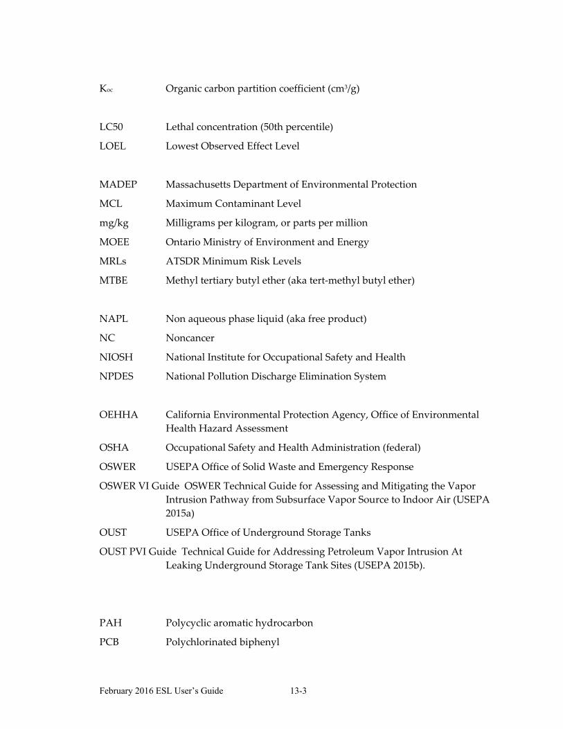
February 2016 ESL User’s Guide 13-3
Koc Organic carbon partition coefficient (cm3/g)
LC50 Lethal concentration (50th percentile)
LOEL Lowest Observed Effect Level
MADEP Massachusetts Department of Environmental Protection
MCL Maximum Contaminant Level
mg/kg Milligrams per kilogram, or parts per million
MOEE Ontario Ministry of Environment and Energy
MRLs ATSDR Minimum Risk Levels
MTBE Methyl tertiary butyl ether (aka tert‐methyl butyl ether)
NAPL Non aqueous phase liquid (aka free product)
NC Noncancer
NIOSH National Institute for Occupational Safety and Health
NPDES National Pollution Discharge Elimination System
OEHHA California Environmental Protection Agency, Office of Environmental
Health Hazard Assessment
OSHA Occupational Safety and Health Administration (federal)
OSWER USEPA Office of Solid Waste and Emergency Response
OSWER VI Guide OSWER Technical Guide for Assessing and Mitigating the Vapor
Intrusion Pathway from Subsurface Vapor Source to Indoor Air (USEPA
2015a)
OUST USEPA Office of Underground Storage Tanks
OUST PVI Guide Technical Guide for Addressing Petroleum Vapor Intrusion At
Leaking Underground Storage Tank Sites (USEPA 2015b).
PAH Polycyclic aromatic hydrocarbon
PCB Polychlorinated biphenyl

February 2016 ESL User’s Guide 13-4
PCE Tetrachloroethene (aka perchloroethylene)
PEL Permissible Exposure Limit
PPRTV USEPA Provisional Peer‐Reviewed Toxicity Value
PRG USEPA Preliminary Remediation Goal (now RSL)
PVI Petroleum vapor intrusion
RfC Inhalation Reference Concentration (noncarcinogens)
RfD Oral Reference Dose (noncarcinogens), also RfDo
Region 2 The region overseen by the San Francisco Bay Regional Water Quality
Control Board or the region itself
REL Recommended Exposure Limit
Regional Water Board California Environmental Protection Agency, San Francisco Bay
Regional Water Quality Control Board
RSL USEPA Regional Screening Level (formerly PRG)
SFo Cancer oral slope factor
SGC Silica gel cleanup
State Water Board California Environmental Protection Agency, State Water Resources
Control Board
STLC Soluble Threshold Limit Concentration (for liquids)
Subslab Subslab soil gas. Soil gas collected immediately beneath a concrete slab.
TBA Tertiary butyl alcohol
TCE Trichloroethene
TCE Framework Interim Framework for Assessment of Vapor Intrusion at TCE‐
Contaminated Sites in the San Francisco Bay Region (Regional Water
Board 2014)
TEF Toxicity equivalence factor
TEQ Toxic equivalents
TMDL Total Maximum Daily Load
TPH Total petroleum hydrocarbons
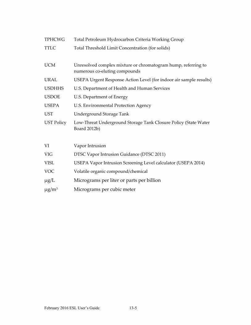
February 2016 ESL User’s Guide 13-5
TPHCWG Total Petroleum Hydrocarbon Criteria Working Group
TTLC Total Threshold Limit Concentration (for solids)
UCM Unresolved complex mixture or chromatogram hump, referring to
numerous co‐eluting compounds
URAL USEPA Urgent Response Action Level (for indoor air sample results)
USDHHS U.S. Department of Health and Human Services
USDOE U.S. Department of Energy
USEPA U.S. Environmental Protection Agency
UST Underground Storage Tank
UST Policy Low‐Threat Underground Storage Tank Closure Policy (State Water
Board 2012b)
VI Vapor Intrusion
VIG DTSC Vapor Intrusion Guidance (DTSC 2011)
VISL USEPA Vapor Intrusion Screening Level calculator (USEPA 2014)
VOC Volatile organic compound/chemical
μg/L Micrograms per liter or parts per billion
μg/m3 Micrograms per cubic meter


Appendix A Tier 3 Risk Assessment Information


1
Appendix A: Tier 3 Assessments
For a Tier 3 assessment, alternative models and assumptions are used and fully justified
to develop a detailed, comprehensive environmental risk assessment. For human health
risk assessments, Tables A‐1 and A‐2 list relevant guidance from USEPA and DTSC,
respectively. These are not endorsements or requirements, but are pertinent to risk
assessments submitted to the Regional Water Board.
Regional Water Board staff recommends that, prior to submission of Tier 3 assessments,
the overseeing regulatory agency be consulted or a work plan be submitted. This
significantly reduces the effort by all parties in moving forward.
Table A‐1 – Select USEPA Documents Relevant for Human Health Risk Assessments
Year Title1989 Risk Assessment Guidance for Superfund. Volume I, Human Health Evaluation
Manual (Part A)
1991a Risk Assessment Guidance for Superfund. Volume I, Human Health Evaluation
Manual (Part B, Development of Risk‐based Preliminary Remediation Goals)
1991b Risk Assessment Guidance for Superfund. Volume I, Human Health Evaluation
Manual (Part C, Risk Evaluation of Remedial Alternatives)
1996b Soil Screening Guidance: Technical Background Document
2001 Risk Assessment Guidance for Superfund. Volume I, Human Health Evaluation
Manual (Part D, Standardized Planning, Reporting, and Review of Superfund
Risk Assessments)
2002 Supplemental Guidance for Developing Soil Screening Levels for Superfund Sites
2002 Role of Background in the CERCLA Cleanup Program
2004 Risk Assessment Guidance for Superfund. Volume I, Human Health Evaluation
Manual (Part E, Supplemental Guidance for Dermal Risk Assessment)
2009 Risk Assessment Guidance for Superfund. Volume I, Human Health Evaluation
Manual (Part F, Supplemental Guidance for Inhalation Risk Assessment)
2011 Exposure Factors Handbook: 2011 Edition
2014 Memorandum: Determining Groundwater Exposure Point Concentrations,
Supplemental Guidance. OSWER Directive 9283.1‐42
2014 Human Health Evaluation Manual, Supplemental Guidance: Update of Standard
Default Exposure Factors. OSWER Directive 9200.1‐120

2
Table A‐2 – Select DTSC Documents Relevant for Human Health Risk AssessmentsYear Title1997 Selecting Inorganic Constituents as Chemicals of Potential Concern at Risk
Assessments at Hazardous Waste Sites and Permitted Facilities. Final Policy.
2009 Human Health Risk Assessment Note 2 – Interim, Issue: Remedial Goals for
Dioxins and Dioxin‐like Compounds for Consideration at California Hazardous
Waste Sites
2014a Human Health Risk Assessment Note 5, Issue: Health‐Based Indoor Air Screening
Criteria for Trichloroethylene (TCE)
2014b Human Health Risk Assessment Note 1, Issue: Recommended DTSC Default
Exposure Factors for Use in Risk Assessment at California Hazardous Waste Sites
and Permitted Facilities
2016 Human Health Risk Assessment Note 3, Issue: DTSC‐Modified Screening Levels
(DTSC‐SLs)
2015a Human Health Risk Assessment Note 4, Issue: Screening Level Human Health
Risk Assessments
2015b Preliminary Endangerment Assessment Guidance Manual
2016 Human Health Risk Assessment Note 3, Issue: DTSC‐Modified Screening Levels
(DTSC‐SLs)

Appendix B Technical Resource Document: Default Subslab Soil Gas and Soil Gas to Indoor Air Attenuation Factors in the ESLs


SanFranciscoBayRegionalWaterQualityControlBoard
TechnicalResourceDocument:DefaultSubslabSoilGasandSoilGastoIndoorAirAttenuationFactorsintheESLs
February 16, 2016
Prepared by: Ross Steenson, CHG Nicole Fry, PhD Cheryl Prowell, PE Approved by: Stephen Hill, Toxics Cleanup Division Chief Terry Seward, Groundwater Protection Division Chief

Table of Contents Executive Summary ...................................................................................................................... 1
1. Introduction .................................................................................................................... 1
2. Background .................................................................................................................... 1
a. Characteristics of Subslab Soil Gas ............................................................................... 1
b. Soil Gas Attenuation Factors in Prior Versions of the ESLs ........................................... 2
3. Conceptual Model for Subsurface Vapor Entry into Buildings ........................................ 3
a. Driving Forces for Vapor Entry ....................................................................................... 3
b. Soil Vapor Entry Rates ................................................................................................... 4
c. Mixing in Indoor Air and Indoor Air Exchange Rates ...................................................... 5
4. Evaluation of Approaches for Calculating Generic Attenuation Factors ......................... 5
a. Model Approach ............................................................................................................. 6
i. USEPA Vapor Intrusion Model ....................................................................................... 6
ii. Vapor Flux Approach Used in the 2003 through 2008 ESLs .......................................... 6
iii. Climate-Adjusted Vapor Flux Approach ......................................................................... 6
iv. Review of Model Approaches ......................................................................................... 7
b. Empirical Approach ........................................................................................................ 7
i. Description of the USEPA Vapor Intrusion Database ..................................................... 7
ii. Review and Analysis of Empirically-Derived Subslab Attenuation Factors .................... 9
5. Selected Approach for Generic Subslab/ Soil Gas Attenuation Factors in the ESLs ... 10
a. Climate-Specific Generic Subslab and Soil Gas Attenuation Factors .......................... 11
b. Prerequisites for Use of the Subslab Attenuation Factor ............................................. 11
i. Intact Foundation .......................................................................................................... 12
ii. Properly Collected Subslab Data .................................................................................. 12
c. Development of Site-Specific, Generic SSIA AFs ........................................................ 12
6. Subslab Line of Evidence and Multiple Lines of Evidence Approach ........................... 13
7. References ................................................................................................................... 13
8. Acronyms and Abbreviations ........................................................................................ 15

List of Tables
1 – Summary of Climate-Adjusted, Vapor Flux Subslab to Indoor Air Attenuation Factors
2 – Attenuation Factors Used for Developing Subslab and Soil Gas ESLs
List of Figures
1 – Generic Subslab Soil Gas to Indoor Air Attenuation Factor Used to Develop the Subslab Soil Gas ESL for a Residential Scenario Following the Vapor Flux Model
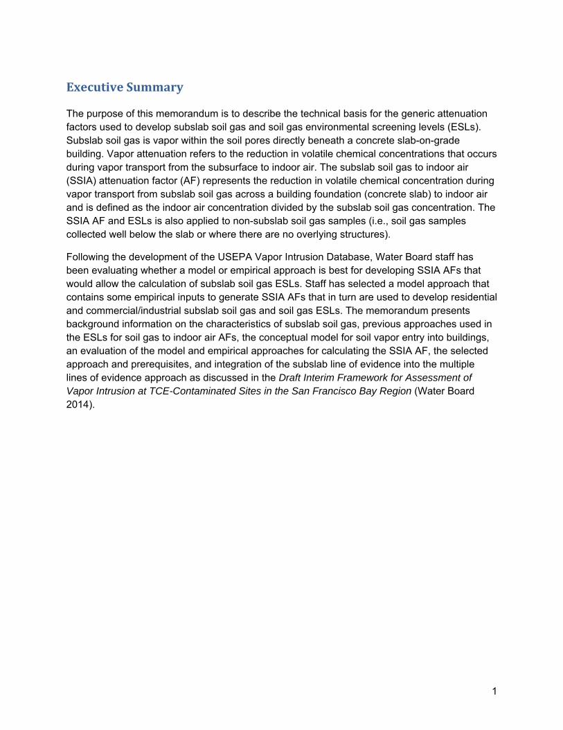
1
ExecutiveSummary
The purpose of this memorandum is to describe the technical basis for the generic attenuation factors used to develop subslab soil gas and soil gas environmental screening levels (ESLs). Subslab soil gas is vapor within the soil pores directly beneath a concrete slab-on-grade building. Vapor attenuation refers to the reduction in volatile chemical concentrations that occurs during vapor transport from the subsurface to indoor air. The subslab soil gas to indoor air (SSIA) attenuation factor (AF) represents the reduction in volatile chemical concentration during vapor transport from subslab soil gas across a building foundation (concrete slab) to indoor air and is defined as the indoor air concentration divided by the subslab soil gas concentration. The SSIA AF and ESLs is also applied to non-subslab soil gas samples (i.e., soil gas samples collected well below the slab or where there are no overlying structures).
Following the development of the USEPA Vapor Intrusion Database, Water Board staff has been evaluating whether a model or empirical approach is best for developing SSIA AFs that would allow the calculation of subslab soil gas ESLs. Staff has selected a model approach that contains some empirical inputs to generate SSIA AFs that in turn are used to develop residential and commercial/industrial subslab soil gas and soil gas ESLs. The memorandum presents background information on the characteristics of subslab soil gas, previous approaches used in the ESLs for soil gas to indoor air AFs, the conceptual model for soil vapor entry into buildings, an evaluation of the model and empirical approaches for calculating the SSIA AF, the selected approach and prerequisites, and integration of the subslab line of evidence into the multiple lines of evidence approach as discussed in the Draft Interim Framework for Assessment of Vapor Intrusion at TCE-Contaminated Sites in the San Francisco Bay Region (Water Board 2014).

1
1. Introduction
Subslab soil gas is vapor within the soil pores directly beneath a concrete slab-on-grade building foundation. Vapor attenuation refers to the reduction in volatile chemical concentrations that occurs during vapor transport from the subsurface to indoor air. The subslab soil gas to indoor air (SSIA) attenuation factor (AF) is the indoor air concentration divided by the subslab soil gas (subslab) concentration as shown in Equation 1a below. It allows for the development of subslab screening levels by relating subslab concentrations to the indoor air screening level as shown in Equation 1b:
SSIA AF = Indoor Air Concentration / Subslab Soil Gas Concentration [Equation 1a]
Subslab Soil Gas Screening Level = Indoor Air Screening Level / SSIA AF [Equation 1b]
Following the development of the USEPA Vapor Intrusion Database, Water Board staff has been evaluating whether a model or empirical approach is best for developing a SSIA AF that would allow for the calculation of generic subslab soil gas screening levels. This memorandum documents our evaluation and technical justification for the adoption of a model-based approach, which we call the vapor flux (VF) approach. This approach is based on the vapor-entry-to-building component of the Johnson and Ettinger model (JEM Johnson and Ettinger 1991) and includes empirical input values.
The memorandum presents background information on the characteristics of subslab soil gas, previous approaches used in the Water Board’s Environmental Screening Levels (ESLs) for soil gas to indoor air (SGIA) AFs, the conceptual model for soil vapor entry into buildings, an evaluation of the model and empirical approaches for calculating the SSIA AF, the selected approach and prerequisites, and integration of the subslab line of evidence into the multiple lines of evidence approach as discussed in the Draft Interim Framework for Assessment of Vapor Intrusion at TCE-Contaminated Sites in the San Francisco Bay Region (Water Board 2014).
2. Background
a. CharacteristicsofSubslabSoilGasSubslab concentrations are the result of diffusion from the volatile organic compound (VOC) VOC vapor source, which is typically groundwater except near source areas where the vapor source can be vadose zone soil as well. Subslab concentrations are controlled by the characteristic length ratio of the depth of the foundation divided by the depth of the VOC vapor source (Yao et al. 2012) and the slab capping effect (Shen et al. 2014). In part due to the capping effect, areas of high subslab VOC concentrations do not necessarily correspond to areas of high vapor flow or entry into a building (Pennell et al. 2009).
Numerous vapor intrusion studies indicate that the subslab concentrations can vary laterally by several orders of magnitude (McHugh et al. 2007; Luo et al. 2009; Yao et al. 2013; Brewer et al.

2
2014). In addition to this spatial variability, there is often temporal variability due to indoor-outdoor pressure reversals that can drive indoor air into the subsurface and dilute subslab concentrations (McHugh et al. 2006). As a result of both spatial and temporal variability, the number of spatially-separated subslab samples as well as the number of samples collected over time from the same sampling point necessary to characterize the mean subslab concentration can be quite large. For instance, McHugh et al. (2007) estimated that it could take up to 10 spatially-separated subslab sample points to estimate the mean subslab concentration to within 50 percent (%) of the true mean. This variability translates to uncertainty in the subslab line of evidence since most investigations lack this level of sampling resolution (see Section 6 for discussion of the subslab line of evidence).
b. SoilGasAttenuationFactorsinPriorVersionsoftheESLsThe 2008 and prior versions of the ESLs used either of two model-based approaches for calculating a generic SGIA AF:
2001 ESLs – JEM as programmed into Microsoft Excel by USEPA (Johnson 2002);
2003, 2005, and 2008 ESLs – the VF approach. The SGIA AF was 0.001 (1/1,000). No distinction was made between AFs for subslab soil gas samples and non-subslab or exterior soil gas samples (i.e., soil gas samples collected well below the slab or where there are no overlying structures) prior to the 2013 ESLs; the SGIA AF applied to all soil gas samples. The majority of the attenuation was treated as taking place as subsurface vapors passed from the soil across a concrete slab-on-grade where the soil was dry sand.
Between 2010 and 2011, Water Board staff considered adoption of an empirical SSIA AF of 0.05 (1/20) developed from a preliminary version of USEPA’s Vapor Intrusion Database (VI Database; USEPA 2008). This AF also would have been applied to both subslab and non-subslab soil gas, again the majority of attenuation being the result of transport across a concrete slab-on-grade where the soil was dry sand.
As part of that 2010/2011 effort, Water Board staff solicited input from an outside advisory group. The experts’ comments reflected a variety of concerns regarding the VI Database such as: 1) appropriateness of relying on a national database given California’s climate as well as the San Francisco Bay area’s climate; 2) the inability to adequately distinguish between indoor sources of VOCs versus subsurface sources of VOCs and appropriately exclude data impacted by indoor air sources; and 3) the data filtering process removed data pairs where indoor air sample concentrations were less than paired subsurface vapor concentrations which effectively biased the results towards larger AFs (i.e., less attenuation).
In 2013, Water Board staff updated the ESLs and harmonized the soil gas AFs with the DTSC Vapor Intrusion Guidance (VIG; DTSC 2011). This included adopting a residential SGIA AF of 0.002, which had been developed by OEHHA using the soil-to-indoor-air version of the JEM (OEHHA 2004). OEHHA modeled vapor intrusion to indoor air from a location six inches below a concrete slab (i.e., subslab) immediately above the contamination source. We also reduced in the default residential indoor air exchange rate (AER) from 1.0 change per hour (as it had been

3
in all previous ESL versions) to 0.5/hour, and the commercial/industrial AER from 2.0/hour to 1.0/hour.
However, based on evaluation of the comments received from the advisory group in 2011 as well as the literature and other information, an empirically-derived subslab AF was not adopted. As stated in the December 2013, ESL Frequently Asked Questions,
a “1:20 attenuation factor between indoor air and subslab may not be appropriate for sites in our region. It is based on EPA’s empirical data for sites across the country, many of which have different conditions than are found in our region (e.g., basements and long/cold winters [indoor heating season] that can emphasize the advective flow component of vapor intrusion). As a practical matter, we think that most sites will exceed subslab screening levels based on the 1:20 attenuation factor, meaning that most sites will need to perform Tier 2 assessments. Therefore, the February 2013 ESLs omit subslab ESLs and the cover memo recommends a Tier 2 (site specific) assessment to derive subslab screening levels, as needed.”
3. ConceptualModelforSubsurfaceVaporEntryintoBuildings
The following is a summary of our understanding of how subsurface vapors intrude into buildings and are mixed including the driving forces for vapor entry, vapor entry rates, and mixing in buildings and indoor air exchange rates.
a. DrivingForcesforVaporEntryThere are two components to the transport of contaminated subsurface soil vapor into buildings: 1) vapor transport in the subsurface from the VOC vapor source toward the building; and 2) subsurface vapor entry into the building. After entry, vapors are mixed with indoor air.
These two components are dominated by different processes. Overall, vapor transport in the subsurface is controlled by phase partitioning, diffusion, and advection (USEPA 2012a). However, it is widely accepted that diffusion dominates in the transport of contaminated vapors from the subsurface VOC vapor source (vadose zone soil or groundwater) towards a building and that, near a building, advection dominates and is the process by which soil vapor is transported into the building typically considered to be via cracks or other adventitious openings (Yao et al. 2013; USEPA 2015).
Advective subsurface vapor transport into buildings is driven by the preferential differential between the soil gas pressure and the air pressure inside a building (∆P). This pressure difference is the result of the stack effect1 and wind effect2 (Song et al. 2014). In addition, the
1 The stack effect is caused by differences in the temperature of outdoor air, indoor air, and intruding subsurface
vapor. As heated indoor air rises and leaves the building through gaps and cracks in the roof and walls, cooler subsurface air is drawn up into the building through the slab. Robinson and Sextro (1997) found that the stack effect was associated with about ∆P = -0.15 Pascals.

4
operation of mechanical ventilation or heating systems (e.g., heating, and air-conditioning systems or HVAC, furnaces, fans, etc.) can also result in pressure differences that drive inward or outward flow (Hers et al. 2001). While the typical range of ∆P is -10 pascals (Pa) to +10 Pa (Shen et al. 2016), under ambient conditions, sustained ∆P values are typically 0 to -5 Pa (Robinson and Sextro 1997), with -5 Pa being used as conservative value for constant building depressurization (USEPA 2004; DTSC 2011; Brewer et al. 2014). Depressurizations greater than the typical range (e.g., -10 Pa) are associated with extreme weather conditions such as storms or high winds (Robinson and Sextro 1997; Holton et al. 2013; and Song et al. 2014). Potentially, it is these pressure fluctuations that can drive periodic fluctuations in indoor air concentrations that have been detected in the few buildings that have been subjected to continuous monitoring.
In addition to advection, there can be a small component of transport from diffusion or atmospheric pressure differences. Robinson and Sextro (1997) studied radon entry into an experimental basement and measured the flux associated with diffusion, atmospheric pressure fluctuations, and sustained indoor-soil gas pressures. For steady indoor-soil gas pressure differences greater than 1.5 Pa, advective flow dominated and contributions from atmospheric pressure fluctuations and molecular diffusion were negligible. This condition typically occurs during the winter heating season or on windy days, which corresponds to a VI active period per Holton et al. (2013). For steady indoor-soil gas pressure differences less than 1.5 Pa, diffusion and atmospheric pressure fluctuations drove soil vapor entry, with the contribution from the atmospheric pressure fluctuations being about 50% greater than diffusion. These conditions commonly occur during the summer when indoor-outdoor temperature differences are small and winds are light, which corresponds to a VI inactive period per Holton et al. (2013).
b. SoilVaporEntryRatesThe pressure-driven soil vapor entry rate (Qsoil in the JEM) represents the rate at which subsurface vapors enter the building through concrete slab foundation cracks or walls. It is a critical determinant of the indoor air concentration (Johnson 2002) and controlled by ∆P. The range of typical Qsoil values is 1 to 10 L/min (USEPA 2004; Song et al. 2011; DTSC 2011; Song et al. 2014; and Brewer et al. 2014). A value of 5 L/min is recommended by USEPA (2004) for coarse-grained soil and a default-size home.3 The corresponding ∆P is -4 Pa.
Typically, Qsoil increases as ∆P increases although VOC vapor transport into a building can become limited by the rate at which VOC mass diffuses from the VOC vapor source to the soil below the building (USEPA 2012a; Shen et al. 2016). A study by Fischer et al. (1996) demonstrated this Qsoil – ∆P relationship in the course of investigated soil gas transport of petroleum VOCs into a 50 square meter building. Part of the study included measurement of the building ventilation rate (Qbuilding) and Qsoil using forced depressurization with a fan designed for testing ventilation ducts and sulfur hexafluoride as a tracer gas. The ambient Qsoil was predicted 2 The wind effect is the result of the differential pressure from wind load on a building, higher pressure on the
upwind side than the downwind side of the building. Thus, air leaks into the building on the upwind side and leaks out on the downwind side.
3 Default-size home refers to a residential, slab-on-grade building with 100 square-meter footprint and height of 2.44 meters, which results in an enclosed space volume of 244 cubic meters or 244,000 liters. See USEPA (2004) for further information.

5
to be in the range of 0.4 L/min and 2.1 L/min based on an estimate of depressurization due to average wind loading (∆P between 1 and 4 Pa). Depressurization was imposed at -10 Pa and -75 Pa and the measured Qsoil values were 3.5 L/min and 14 L/min, respectively. Note that, if the Qsoil values were proportionally adjusted to a 100 m2 footprint (default size house),4 the scaled Qsoil values would be 7 L/min (-10 Pa) and 28 L/min (-75 Pa). The authors described the dependence of Qsoil on building depressurization as approximately linear.
c. MixinginIndoorAirandIndoorAirExchangeRatesAs soil gas migrates into a building, it is mixed with indoor air, which is exchanged via infiltration/leakage, natural ventilation, and/or mechanical ventilation. The indoor air exchange rate is rarely measured in vapor intrusion studies, but has been studied for other reasons (Brewer et al. 2014). Studies between the 1970s and 1990s indicated that, under natural conditions (no mechanical ventilation), average AERs can be about 0.25/h, which is the same value recommended by USEPA (2004). Subsequent, more detailed studies suggest regional variations based on climate, with a US median value of 0.51/h. The USEPA Exposure Factors Handbook (USEPA 2011) provides a discussion of various studies of AERs as does the Supplement to Brewer et al. (2014). For example, the Yamamoto et al. (2010) study between 2000 and 2001 evaluated AERs for residences in Los Angeles. Results of that study indicated a median AER of 0.87/h overall with seasonal differences of 1.13/h (summer) and 0.61/h (winter).
In models, AER is usually set as a fixed value (Shen et al. 2016): 0.5/h Johnson and Ettinger (1991); 0.25/h (USEPA 2004); 0.5/h (Abreu and Johnson 2006); 0.5/h (DTSC 2011); and 0.25/h (Yao et al. 2011). AER was monitored in a single family home for about 18 months by Holton et al. (2013). The AER varied between about 0.2/h to 1.5/h.
Shen et al. (2016) evaluated transient effects on indoor air concentrations from AER variations using a three-dimensional model, and concluded that when Qsoil and AER are in phase, which is typical, indoor air concentrations varied about an order of magnitude. Both modeling and field studies have demonstrated that there is a positive correlation between Qsoil and AER (Cavallo et al. 1992; Song et al. 2014). This is because, as Qsoil increases, the stack effect increases, which increases Qbuilding. The increase in Qbuilding acts to offset the Qsoil increase.
4. EvaluationofApproachesforCalculatingGenericAttenuationFactors
There are two approaches for generating SSIA and groundwater to indoor air screening levels: models and, more recently, empirical data (Song et al. 2014). The most common model that has been used to generate generic screening levels is the JEM as programmed into Microsoft Excel by USEPA (Johnson 2002). The empirical approach for generating generic AFs relies on field data compiled into a database (e.g., VI Database; USEPA 2012b).
4 See Table 3, footnote 5 of the VIG (DTSC 2011).

6
a. ModelApproach
i. USEPAVaporIntrusionModel
The JEM calculates AFs based on soil, building, as well as chemical-specific factors, and exposure parameter inputs It is a one-dimensional analytical fate and transport model of vapors into indoor air (USEPA, 2004). The model combines source zone partitioning, vapor transport through the vadose zone, vapor transport across building foundation, and enclosed-spacing mixing to estimate the vapor attenuation factor (called the Infinite Source Indoor Air Coefficient on the INTERCALCS worksheet), which relates the indoor air concentration to the vapor concentration at the source (Johnson 2002). The model’s intended use is for screening purposes. It is based on a number of simplifying assumptions, which are discussed in the User’s Guide for Evaluating Subsurface Vapor Intrusion into Buildings (USEPA 2004).
ii. VaporFluxApproachUsedinthe2003through2008ESLs
The VF approach for estimating SSIA attenuation is based on the subsurface vapor flow into a building through the foundation and the building ventilation rate. As previously stated, this approach is based on the vapor-entry-to-building component of the Johnson and Ettinger model. The basic equation for the AF with a residential example from the 2003 to 2008 ESLs is presented below:
SSIA AF = Qsoil / (Qsoil+ Qbuilding) [Equation 2]
SSIA AFresidential = (5L/min)/(5L/min + 4,000 L/min) = 0.001 or 1E-03. [Equation 3]
where:
Qsoil = Pressure-driven volumetric flow of soil gas into building. The USEPA-recommended default value for Qsoil is 5 L/minute (USEPA 2004; DTSC 2011), based on the default-size home.
Qbuilding = Volumetric flow rate of outdoor air exchanged into the default-size home (volume of 244,000 L) with an AER of 1/hour, which results in 4,000 L/min.
iii. Climate‐AdjustedVaporFluxApproach
A climate-adjusted VF approach was proposed by Brewer et al. (2014). This paper identifies a number of shortcomings associated with the USEPA Vapor Intrusion Database for deriving a simple generic SSIA AF and presents an updated VF approach as an alternative for deriving or “estimating” generic subslab AFs. The VF equation remains the same as Equation 2 above, but has been updated with regional-climate-adjusted inputs for Qsoil and AER; we call this updated approach the climate-adjusted VF approach.
Brewer et al. (2014) divided the United States into four vapor intrusion risk (VIR) regions based on average building leakage rates and associated AERs and vapor entry rates. The climate-adjusted vapor entry rate is based on the average number of heating and cooling days in four VIR regions and a default AER for each region. Table 1 illustrates the inputs and the SSIA AF for each VIR region.

7
Table 1 – Summary of Climate-Adjusted, Vapor Flux Subslab to Indoor Air Attenuation Factors (after Brewer et al. 2014)
VIR Region Climate-Adjusted Vapor Entry Rate
(L/min) Default AER (1/hour) SSIA AF
A (Cold) 4.5 0.35 0.0032
B (Warm) 4.0 0.50 0.0020
C (Mediterranean) 3.4 1.0 0.0008
D (Tropical) 2.0 1.0 0.0005
The San Francisco Bay Region straddles VIR B and VIR C in Table 2, suggesting that a SSIA AF between 0.002 (1/500) and 0.0008 (1/1250) would be appropriate.
iv. ReviewofModelApproaches
Problems associated with the use of models such are the result of over-simplification. Additional problems can arise from lack of accuracy of inputs. Disadvantages of the vapor flux approach are: (1) that the inputs are not measured during vapor intrusion investigations; and (2) both Qsoil and AER are known to vary, but are represented as conservative averages based on published data. Nevertheless, the model reflects conventional understanding of how vapors intrude into buildings, the resulting SSIA AF is consistent with those reported from a number of field studies of concrete slab-on-grade buildings: 0.002 (King et al. 2010; 0.0002-0.0003 McHugh et al. 2004; 0.0026 McDonald and Wertz (2006); and 0.003 for the northeastern United States (Song et al. 2014).
b. EmpiricalApproach
i. DescriptionoftheUSEPAVaporIntrusionDatabase
An empirical approach for generic AFs involves the compilation and evaluation of field data. The VI Database is the best known example of an empirical database. The VI Database was developed using data collected by others during the early years of vapor intrusion investigations (e.g., the most recent data are from 2006). The data are indoor air, subslab soil gas, deep/exterior soil gas, and groundwater and were collected from 913 buildings, 41 sites, and 15 states. The rest of our discussion about the VI Database is focused to derivation of the SSIA AF.
The VI Database contains 1,582 paired subslab soil gas and indoor air measurements. The data were paired considering proximity and temporal concurrency. The spatial proximity criterion for subslab soil gas and indoor air samples was whether the samples were from the same building. The temporal concurrency criterion for subslab soil gas and indoor air samples was whether the samples were collected within 48 hours of each other.

8
The subslab-indoor air data pairs were initially filtered using three screens, collectively called the Baseline Screens:
Chlorinated VOCs (CVOCs) in Residences Screen – Excluded non-CVOC data and non-residential buildings thus focusing the remaining dataset to CVOCs and residential buildings. This removed 351 data pairs.
Subsurface Concentration Screen – Excluded data pairs where the subslab concentration was less than reporting limits. This removed 24 data pairs.
Data Consistency Screen – Excluded samples where the field notes indicated the presence of indoor sources (background) of CVOCs, the indoor air concentrations were greater than the subslab soil gas concentrations, or AFs for individual chemicals were not consistent with other chemicals reported for the same samples. This removed 440 data pairs.
Following application of the Baseline Screens, 767 data pairs remained. Two additional screens were developed, but these screens are not applied together, rather they are alternatives:
Indoor Air Screen – Excludes samples with indoor sample concentrations that were less than reporting limits or less than the 90th percentile of background levels presented in the USEPA Background Indoor Air Concentrations of Volatile Organic Compounds in North American Residences (1990-2005): A Compilation of Statistics for Assessing Vapor Intrusion (USEPA 2011a). This removes 447 data pairs, leaving 320 data pairs total.
Source Strength Screen – Excludes subslab soil gas samples with concentrations less than 50 times the 90th percentile of background levels (USEPA 2011). This removes 336 data pairs, leaving 431 data pairs total.
USEPA evaluated the advantages and disadvantages of employing the indoor air screen versus the source strength screen as the final step. Because the AF distributions that remained after applying the Source Strength Screen were close to lognormal distributions and exhibited less of the bimodal distortion that may have been induced by background contributions, the Source Strength Screen (subslab > 50x background) was selected. Then, USEPA calculated median and 95th percentile SSIA AFs of 0.003 (1/300) and 0.03 (1/30), respectively.
The USEPA-recommended generic SSIA AF is 0.03 (1/33; USEPA 2015). This same value is recommended for the non-subslab soil gas. Use of the 95th percentile value was intended to account for temporal and spatial variability in indoor air and subsurface vapor concentrations. USEPA (2012b and 2015) points out that the upper-bound value (95th percentile) of 0.03 is similar to that derived using a low AER (0.18/h; USEPA 2011) and high soil vapor entry rate (10 L/min) for a residential building volume of 154 cubic meters, resulting in an SSIA AF of 0.02.

9
ii. ReviewandAnalysisofEmpirically‐DerivedSubslabAttenuationFactors
The VI Database has been subject to a number of reviews (McHugh et al. 2007; Song et al. 2011; Yao et al. 2013; Song et al. 2014; Brewer et al. 2014; and Yao et al. 2015). Criticisms have largely focused on the SSIA AF. In evaluating an empirical approach for deriving SSIA AFs for possible use in the ESLs we considered the following:
Climate Variation – Given California’s milder climate, it may not be appropriate to rely on a national database that represents buildings with lower AERs and greater indoor-soil gas under pressurization due to colder weather (heating).
Challenge of Distinguishing between Indoor and Subsurface Sources of VOCs – It is now well recognized that it is more challenging to distinguish between indoor sources of VOCs versus subsurface sources of VOCs and appropriately exclude data impacted by indoor air sources, but there are techniques that can be employed to distinguish indoor versus subsurface vapor sources (Song et al. 2011; NAVFAC 2013). However, these techniques were developed after the data in the VI Database were collected. Some authors have focused on identifying subslab concentrations where it is possible to reasonably attribute indoor air concentrations to be primarily the result of intruding subsurface vapors. Song et al. (2011) evaluated the VI Database and concluded that subsurface concentrations should be at least 300 times higher than potential background indoor air levels to reduce high bias due to indoor sources of VOCs. Yao et al. (2015) similarly concluded that, for subslab concentrations below 500 µg/m3, the source of low-level indoor air VOC concentrations cannot be definitively attributed to subsurface vapor intrusion.
Mass Balance Problem – As discussed by Song et al. (2011), there is a mass balance problem with the SSIA AF of 0.03 considering Qsoil and AER. For the default-size home, using reasonable values of Qsoil (5 L/min) and AER (0.5/hour), the SSIA AF would be 0.0025. To achieve a SSIA AF of 0.03 for the default-size home with the same AER, Qsoil would have to be 70 L/min, which is not consistent with the conceptual model for soil vapor entry and typical ∆P conditions. Coupling a low AER and high Qsoil value, as done in Section 5.1 of the VI Database report (USEPA 2012b), is implausible based on the physics driving soil vapor entry (Hers et al. 2001; Song et al. 2014; and Brewer et al. 2014).
Lack of Spatial and Temporal Control in the VI Database – The SSIA AF for a building represents the true or average (mean) attenuation across the slab for an exposure scenario. Most buildings in the VI Database only had one subslab soil gas sample and one indoor air sample (i.e., single data pair) (Brewer et al. 2014). The SSIA AF inferred from a single data pair is subject to a potentially very large error (deviation from the true AF) due to spatial and temporal variability. The statistical evaluation of the VI Database addressed the variability between buildings rather than the variability and error within single data points (Brewer et al. 2014). The use of statistics did not resolve the error resulting from the lack of spatial and temporal control in the VI Database (McHugh et al. 2007; Brewer et al. 2014). Based on an evaluation by McHugh et al. (2007), the use of upper-bound statistics (e.g., 95% UCL) in a dataset with these errors results in an over-estimated and overly conservative AF, as further described below.
McHugh et al. (2007) conducted a study of the spatial and temporal variability at two sites. This work involved three components: 1) a field study to statistically characterize the spatial and temporal variability in indoor air and subsurface media samples; and 2) estimation of the number of samples from each medium necessary to adequately

10
characterize the mean concentration; and 3) an evaluation of the effects of the spatial and temporal variability on the measured AFs in the VI Database.
Based on the coefficients of variation (CVs)5 measured for subslab and indoor air at the two study sites, the authors used a Monte Carlo approach to simulate the measurement of AFs. The average subsurface VOC concentration was set as 1,000 times the average indoor concentration, so that the average true AF would be 0.001. The authors generated 5,000 AFs based on simulated measurements from these populations. The Monte Carlo simulation indicated that the variability in VOC concentration resulted in a 95th percentile AF that is 6.2 times higher than the true AF in a database of AFs based on single paired subslab and indoor air measurements. The authors concluded that the 95th percentile subslab AFs selected by the USEPA are likely to be significantly more conservative than would be expected if the impact of spatial variability were better controlled through better characterization of the average subslab and indoor air concentrations.
5. SelectedApproachforGenericSubslab/SoilGasAttenuationFactorsintheESLs
Although Water Board staff typically prefers empirical approaches over model approaches, in this case, we have significant concerns that using USEPA’s empirically-derived SSIA AF (0.03 or 1/33) is not technically defensible and is not suitable for screening or prioritizing cases. We consider the climate-adjusted vapor flux approach to be consistent with the conceptual model for contaminated subsurface vapor entry into buildings and more scientifically sound for deriving a SSIA AF. Therefore, we are re-adopting the vapor flux approach, but with climate-adjusted inputs, as the basis for deriving SSIA AFs for concrete slab-on-grade buildings. The residential SSIA AF is 0.002 and the commercial/industrial SSIA AF is 0.001.
The residential and commercial/industrial SSIA AFs are also applied to non-subslab soil gas to generate residential and commercial/industrial subslab/soil gas ESLs. This approach conservatively assumes the only attenuation is the result of an intact concrete slab that limits the amount of vapor transported into the building and then the dilution of those vapors by mixing with indoor air. While there can be additional attenuation as vapors diffuse through the soil from a deeper VOC vapor source (primarily due to soil moisture), there are other factors that can result in less attenuation than otherwise expected through the soil profile:
The slab capping effect results from the presence of concrete slabs or buildings that limit VOC release to the atmosphere. Soil gas concentration profiles beneath slabs or buildings show less attenuation than in unpaved areas. Cross-sectional illustrations of this effect are provided in Conceptual Model Scenarios for the Vapor Intrusion Pathway (USEPA 2012a).
5 The coefficient of variation (CV) is a normalized measure of variability that is independent of the measurement
scale and can therefore be compared between sample sets. It is calculated for data sets with three or more matched measurements as the standard deviation divided by the sample mean.
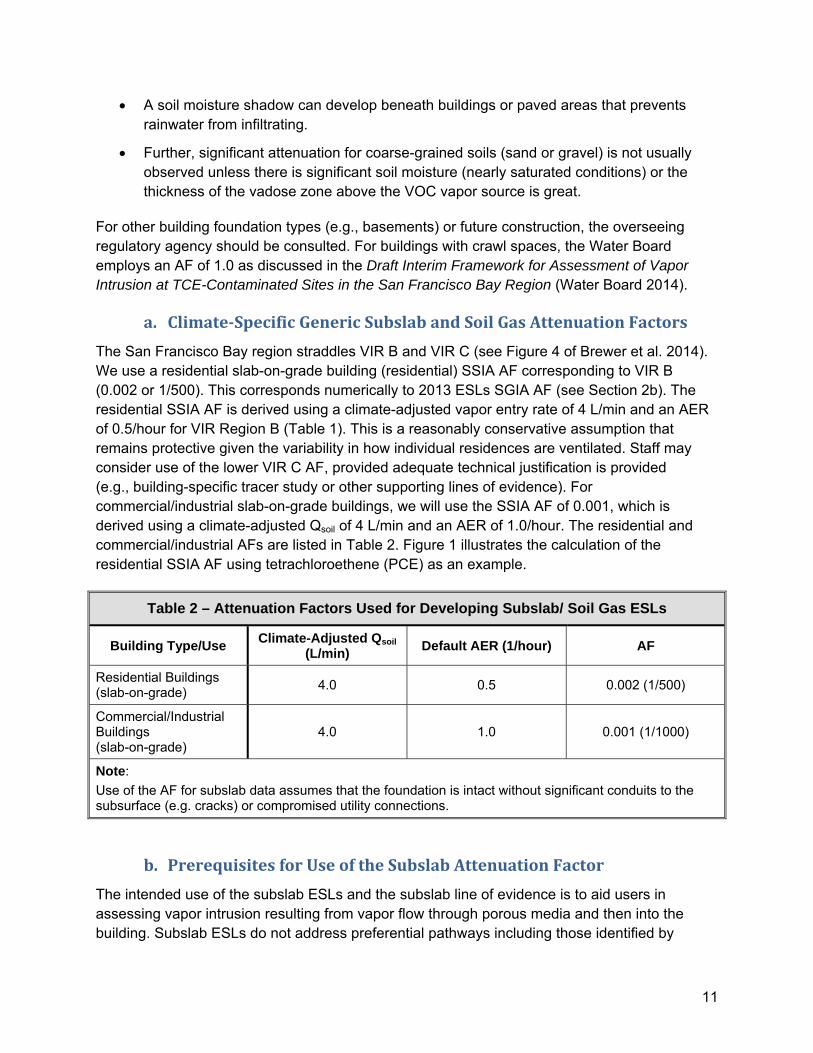
11
A soil moisture shadow can develop beneath buildings or paved areas that prevents rainwater from infiltrating.
Further, significant attenuation for coarse-grained soils (sand or gravel) is not usually observed unless there is significant soil moisture (nearly saturated conditions) or the thickness of the vadose zone above the VOC vapor source is great.
For other building foundation types (e.g., basements) or future construction, the overseeing regulatory agency should be consulted. For buildings with crawl spaces, the Water Board employs an AF of 1.0 as discussed in the Draft Interim Framework for Assessment of Vapor Intrusion at TCE-Contaminated Sites in the San Francisco Bay Region (Water Board 2014).
a. Climate‐SpecificGenericSubslabandSoilGasAttenuationFactorsThe San Francisco Bay region straddles VIR B and VIR C (see Figure 4 of Brewer et al. 2014). We use a residential slab-on-grade building (residential) SSIA AF corresponding to VIR B (0.002 or 1/500). This corresponds numerically to 2013 ESLs SGIA AF (see Section 2b). The residential SSIA AF is derived using a climate-adjusted vapor entry rate of 4 L/min and an AER of 0.5/hour for VIR Region B (Table 1). This is a reasonably conservative assumption that remains protective given the variability in how individual residences are ventilated. Staff may consider use of the lower VIR C AF, provided adequate technical justification is provided (e.g., building-specific tracer study or other supporting lines of evidence). For commercial/industrial slab-on-grade buildings, we will use the SSIA AF of 0.001, which is derived using a climate-adjusted Qsoil of 4 L/min and an AER of 1.0/hour. The residential and commercial/industrial AFs are listed in Table 2. Figure 1 illustrates the calculation of the residential SSIA AF using tetrachloroethene (PCE) as an example.
Table 2 – Attenuation Factors Used for Developing Subslab/ Soil Gas ESLs
Building Type/Use Climate-Adjusted Qsoil (L/min) Default AER (1/hour) AF
Residential Buildings (slab-on-grade)
4.0 0.5 0.002 (1/500)
Commercial/Industrial Buildings (slab-on-grade)
4.0 1.0 0.001 (1/1000)
Note:
Use of the AF for subslab data assumes that the foundation is intact without significant conduits to the subsurface (e.g. cracks) or compromised utility connections.
b. PrerequisitesforUseoftheSubslabAttenuationFactorThe intended use of the subslab ESLs and the subslab line of evidence is to aid users in assessing vapor intrusion resulting from vapor flow through porous media and then into the building. Subslab ESLs do not address preferential pathways including those identified by

12
Pennell et al. (2013) (compromised sanitary sewer connection) or Guo et al. (2015) (land drain in direct connection with groundwater that terminated beneath the slab and did not penetrate the slab). Consequently, it is imperative to gather as much information about the construction, condition, and use of a building and use subslab data (subslab line of evidence) in conjunction with other lines of evidence as discussed in the Draft Interim Framework for Assessment of Vapor Intrusion at TCE-Contaminated Sites in the San Francisco Bay Region (Water Board 2014).
i. IntactFoundation
Use of the AF of 0.002 for subslab data assumes that the building foundation is intact without significant conduits to the subsurface (e.g. cracks) or compromised utility connections. Building drawings should be reviewed and the foundation inspected to the extent possible to support use of the AF for subslab samples. Reports should include information on the age of the building, foundation construction, current foundation condition, building use, other characteristics (basement, garage, etc.), presence of conduits to subsurface (drains, sumps, utility connections), and information on the HVAC and interior partitions. This information should be provided in an appropriate report for review by the overseeing regulatory agency.
ii. ProperlyCollectedSubslabData
The subslab data should be collected consistent with the methods discussed in the Advisory – Active Soil Gas Investigations Advisory – Active Soil Gas Investigations (CalEPA 2015). In addition, sufficient sampling should be performed to address spatial and temporal variability.
Samples should be appropriately located to permit evaluation of relevant exposure of receptors and to determine spatial variability, which can include a combination of targeted and areal or grid-based sampling locations. Targeted sampling can be based on the distribution of source contamination, building occupancy and use, HVAC layout, utility conduits, preferential pathways, and other potential vapor entry points. For areal coverage, some samples should be located near the center of the building (where vapor concentrations are anticipated to be greatest) and others should be located near the edge of the building. McHugh et al. (2007) recommended six spatially-separated subslab samples per building to estimate the mean concentration within 67 percent. Alternatively, high purge volume subslab sampling could be considered to better estimate the mean subslab concentration (McAlary et al. 2010; CalEPA 2015) as another way to address the spatial variability issue.
The Water Board does not accept building-specific attenuation factors based on a single pair of subslab and indoor air samples due to the spatial variability previously discussed. Rather, per McHugh et al. (2007), all available data should be used to develop a single attenuation factor for a building.
Given temporal variability, soil gas (including subslab soil gas) should be monitored over time to determine appropriate exposure point concentrations (USEPA 2015 and DTSC 2011). For instance, consistent with DTSC VIG Appendix G, a final risk determination for a building should not be made without at least two subslab sampling events, at least one should be conducted

13
during a colder weather period or building under pressurization condition. The latter can be ascertained by coupling indoor-soil gas pressure measurements with the subslab soil gas sampling program (USEPA 2015).
c. DevelopmentofSite‐Specific,GenericSSIAAFsThe Water Board will consider the development of an alternative SSIA AF based on building design and climate factors discussed in Brewer et al. (2014) on a site-specific basis. Such a proposal should include adequate technical justification and documentation. Consideration should be given to how an alternative SSIA AF can be validated.
6. SubslabLineofEvidenceandMultipleLinesofEvidenceApproach
Although Water Board staff has selected a subslab AF that is the same as the soil gas AF, staff considers subslab data neither to be a strong line of evidence nor equivalent to the soil gas line of evidence. Rather, subslab data should always be combined with other lines of evidence (Water Board 2014), including other data lines of evidence such as concurrently collected indoor air samples, deeper soil gas and/or groundwater data. We also recommend use of indoor-soil gas pressure measurements because these can help to diagnose whether there is sufficient driving force for subsurface vapor entry at or around the time of sampling (USEPA 2015).
Lines of evidences for vapor intrusion investigations typically are weighted based on proximity to the receptor (building occupant) as well as data representativeness and quality. While subslab data might be more heavily weighted due to proximity to the receptor, that weighting is undermined by the significant concerns regarding data representativeness resulting from spatial and temporal variability. Therefore, unless, the dataset is robust, the subslab line of evidence generally should not be heavily weighted. As stated above, it is important to combine subslab data with other lines of evidence.
7. References
Abreu, D.V. and P.C. Johnson. 2005. Effect of Vapor Source-Building Separation and Building Construction on Soil Vapor Intrusion as Studied with a Three-Dimensional Numerical Model. Environmental Science & Technology 39, pp. 4550-4561.
Brewer, R., J. Nagashima, M. Rigby and M. Schmidt, and Harry O’Neill, 2014. Estimation of Generic Subslab Attenuation Factors for Vapor Intrusion Investigations. Groundwater Monitoring & Remediation, December 15.
CalEPA. 2004. Human-Health-Based Screening Numbers Developed to Aid Estimation of Cleanup Costs for Contaminated Soil. California Environmental Protection Agency. Revised January.
CalEPA. 2015. Advisory – Active Soil Gas Investigations. California Environmental Protection Agency, Department of Toxic Substances Control, Los Angeles Regional Water Quality Control Board, San Francisco Bay Regional Water Quality Control Board. July.
Cavallo, A., K. Gadsby, T.A. Reddy, and R. Socolow. 1992. The effect of natural ventilation on radon and radon progeny levels in houses. Radiation Protection Dosimetry 45, 569–573.

14
DTSC. 2011. Final Guidance for the Evaluation and Mitigation of Subsurface Vapor Intrusion to Indoor Air (Vapor Intrusion Guidance). California Environmental Protection Agency, Department of Toxic Substances Control. October.
Fischer, M.L., A.J. Bentley, K.A. Dunkin, A.T. Hodgson, W.M. Nazaroff, R.G. Sextro, and J.M. Daisey. 1996. Factors Affecting Indoor Air Concentrations of Volatile Organic Compounds at a Site of Subsurface Gasoline Contamination. Environmental Science & Technology 30, pp. 2948-2957.
Hers, I., R. Zapf-Gilje, L. Li, and J. Atwater. 2001. The Use of Indoor Air Measurements to Evaluate Intrusion of Subsurface VOC Vapors into Buildings. Journal of the Air & Waste Management Association 51, pp. 1318–1331.
Holton, C., H. Luo, P. Dahlen, K. Gorder, E. Dettenmaier and P.C. Johnson. 2013. Temporal Variability of Indoor Air Concentrations under Natural Conditions in a House Overlying a Dilute Chlorinated Solvent Groundwater Plume. Environmental Science & Technology 47, pp. 13347-13554.
Johnson, P.C. and R.A. Ettinger. 1991. Heuristic Model for Predicting the Intrusion Rate of Contaminant Vapors into Buildings. Environmental Science & Technology, 25, pp. 1445–1452.
Johnson, P.C. 2002. Identification of Critical Parameters for the Johnson and Ettinger (1991) Vapor Intrusion Model. American Petroleum Institute, Technical Bulletin No. 17, May.
King, J.F., D.W. Shelton and J.R. Blei. 2010. Use of Radon to Determine Attenuation between Subslab and Indoor Air for Vapor Intrusion Evaluation at Military Housing Units at Fort Wainright, Alaska. Proceedings of Air and Waste Management, Vapor Intrusion 2010, September 29-30, 2010, Chicago, IL Annual Conference.
Luo, H., P. Dahlen, P.C. Johnson, T. Peargin, and T. Creamer. 2009. Spatial Variability of Soil-Gas Concentrations near and beneath a Building Overlying Shallow Petroleum Hydrocarbon a Dilute Chlorinate Solvent Groundwater Plume. Ground Water Monitoring & Remediation, 29, no. 1, pp. 81-91.
McAlary, T.A., P.J. Nicholson, L.K. Yik, D. Bertrand, and G. Thrupp. 2010. High Purge Volume Sampling – A New Paradigm for Subslab Soil Gas Monitoring. Groundwater Monitoring & Remediation, 30, no. 2, pp. 73-85.
McHugh, T.E., P.C. De Blanc and R.J. Pokluda. 2006. Indoor Air as a Source of VOC Contamination in Shallow Soils below Buildings. Soil & Sediment Contamination 15, pp. 103–122.
McHugh, T.E., T.N. Nickels, and S. Brock. 2007. Evaluation of Spatial and Temporal Variability in VOC Concentrations at Vapor Intrusion Investigation Sites. In Proceedings of Air & Waste Management Association. Vapor Intrusion: Learning from the Challenges, September 26–28, Providence, Rhode Island, pp. 129–142.
McHugh, T. E., D. E. Hammond, T. Nickels, and B. Hartman. 2008. Use of Radon Measurements for Evaluation of Volatile Organic Compound (VOC) Vapor Intrusion. Environmental Forensics, 9, no. 1, p. 107–114.
NAVFAC (Naval Facilities Engineering Command). 2013. Innovative Vapor Intrusion Site Characterization Methods. February
OEHHA. 2004. Human-Exposure-Based Screening Numbers Developed to Aid Estimation of Cleanup Costs for Contaminated Soil. California Environmental Protection Agency, Office of Environmental Health Hazard Assessment. November (Revised January 2005).
Pennell, K.G., O. Bozkurt, E.M. Suuberg. 2009. Development and Application of a Three-Dimensional Finite Element Vapor Intrusion Model. Journal of the Air & Waste Management Association, 59 (4), pp. 447-460.
Robinson, A.L. and R.G. Sextro. 1997. Radon Entry into Buildings by Atmospheric Pressure Fluctuations. Environmental Science & Technology, 31, pp. 1742-1748.
Shen, R. K.G. Pennell, and E.M. Suuberg. 2014. Analytical Modeling of the Subsurface Volatile Organic Vapor Concentration in Vapor Intrusion. Chemosphere, 95, February, pp. 140-149.

15
Shen, R. and E.M. Suuberg. 2016. Impacts of Changes of Indoor Air Pressure and Air Exchange Rate in Vapor Intrusion Scenarios. Building and Environment, 96, February, pp. 178-187.
Song, S., F.C. Ramacciotti, B.A. Schnorr, M. Bock, and C.M. Stubbs. 2011. Evaluation of USEPA’s Empirical Attenuation Factor Database. Air & Waste Management Association, Emissions Monitoring, pp 16-21.
Song, S., B.A. Schnorr and F.C. Ramacciotti. 2014. Quantifying the Influence of Stack and Wind Effects on Vapor Intrusion. Human and Ecological Risk Assessment, 20, pp. 1345-1358.
USEPA. 2004. User’s Guide for Evaluating Subsurface Vapor Intrusion into Buildings. Prepared by Environmental Quality Management for USEPA Office of Emergency and Remedial Response. February 22.
USEPA. 2008. U.S. EPA’s Vapor Intrusion Database: Preliminary Evaluation of Attenuation Factors. Office of Solid Waste and Emergency Response. March 4.
USEPA. 2011a. Background Indoor Air Concentrations of Volatile Organic Compounds in North American Residences (1990-2005): A Compilation of Statistics for Assessing Vapor Intrusion. EPA 530-R-10-001. Office of Solid Waste and Emergency Response, Washington, DC. June.
USEPA. 2011b. Exposure Factors Handbook: 2011 Edition. EPA 600/R-090/052F. Office of Research and Development, Washington, DC. September.
USEPA. 2012a. Conceptual Model Scenarios for the Vapor Intrusion Pathway. Office of Solid Waste and Emergency Response. February.
USEPA. 2012b. U.S. EPA’s Vapor Intrusion Database: Evaluation and Characterization of Attenuation Factors for Chlorinated Volatile Organic Compounds and Residential Buildings. Office of Solid Waste and Emergency Response. March 16.
USEPA. 2015. OSWER Technical Guide for Assessing and Mitigating the Vapor Intrusion Pathway from Subsurface Vapor Sources to Indoor Air. Office of Solid Waste and Emergency Response. Publication 9200.2-154. June.
Water Board. 2013. User’s Guide: Derivation and Application of Environmental Screening Levels – Interim Final. California Environmental Protection Agency, Regional Water Quality Control Board, San Francisco Bay Region. December.
Water Board. 2014. Draft Interim Framework for Assessment of Vapor Intrusion at TCE-Contaminated Sites in the San Francisco Bay Region. California Environmental Protection Agency, Regional Water Board, San Francisco Bay Region. October 16.
Yamamoto, N., D.G. Shendell, A.M. Winter, and J. Zhang. 2010. Residential Air Exchange Rates in Three U.S. Metropolitan Areas: Results from the Relationship among Indoor, Outdoor, And Personal Air Study 1999–2001. Indoor Air 20, pp. 85–90.
Yao, Y., R. Shen, K.G. Pennell, and E.M. Suuberg. 2011. A Comparison of the Johnson-Ettinger Vapor Intrusion Screening Model Predictions with Full Three-Dimensional Model Results. Environmental Science & Technology 45, pp. 2227−2235.
Yao, Y.J., K.G. Pennell and E.M. Suuberg. 2012. Estimation of Contaminant Subslab Concentration in Vapor Intrusion. Journal of Hazardous Materials 231-232, pp. 10-17.
Yao, Y.J., R. Shen, K.G. Pennell and E.M. Suuberg. 2013. A Review of Vapor Intrusion Models. Environmental Science and Technology 47, pp. 2457-2470.
Yao, Y.J., Y. Wu, E.M. Suuberg J. Provoost, R. Shen, J. Ma, and J. Liu. 2015. Vapor Intrusion Attenuation Factors Relative to Subslab and Source, Reconsidered in Light of Background Data. Journal of Hazardous Materials, 286, pp. 553–561.

IA ESL[0.48 μg/m3]
Figure 1 – Generic Subslab Soil Gas to Indoor Air Attenuation Factor Based on the Vapor Flux Model and Using PCE as an Example.
AF = Attenuation factorESL = Water Board Environmental Screening LevelIA = Indoor airSS = Subslab soil gasSSIA = Subslab soil gas to indoor air
VAPOR FLUX MODELDefault building dimensions = 2.44 meters high by 10 meters long by 10 meters wide.Default building volume = 244 cubic meters or 244,000 liters (L).Default Indoor Air Exchange Rate = 0.5/hour or 122,000 L/hourQbuilding = 122,000 L/hour x (hour/60 min) ~ 2,000 L/min.SSIA AF = Qsoil/(Qsoil + Qbuilding).SSIA AF = 4 L/min/(2,004 L/min) = 0.002.
Building Ventilation Rate(Qbuilding)
[~ 2,000 Liters/minute or L/min]
Vapor Entry Rate (Qsoil)
[4 Liters/min]Subslab Soil Gas ESL = = 240 μg/m3
IA ESL [0.48 μg/m3]SSIA AF [0.002]


Appendix C Model Parameters for Groundwater Vapor Intrusion ESLs Tables of Inputs and Copies of Johnson & Ettinger Model Worksheets for Three Soil Layer Designs (Shallow Groundwater, Deep Groundwater Sand, and Deep Groundwater Fine-Coarse)


Appendix C Table 1Parameters for Shallow GW Scenario ‐ Residential
GW‐to‐Indoor Air ESLsDTSC Vapor Intrusion Model, GW‐SCR, December 2014
Parameter Units Value NotesSoil/Groundwater and Soil Layer ParametersAverage Soil/Groundwater Temperature (T) Celsius 15 From USEPA Userʹs Guide Figure 8.
Depth Below Grade to Bottom of Enclosed Floor (LF) cm 15 DTSC VIG Table 3.
Depth Below Grade to Water Table (LWT) cm 152 Shallow GW model‐specific.
Thickness of Soil Stratum A (hA) cm 152 Shallow GW model‐specific.
Soil Type Used to Estimate Soil Vapor Permeability na Sand (S) USDA SCS soil texture classification. See note (1).
Soil Stratum Directly Above Water Table na A Sand
Stratum A SCS Soil Type na Sand (S) Shallow GW model‐specific.
Stratum A Soil Dry Bulk Density (ρbA) grams/cm3 1.66 Sand default
Stratum A Soil Total Porosity (nA) cm3/cm3 0.375 Sand default
Stratum A Soil Water‐Filled Porosity (ΘwA) cm3/cm3 0.054 Sand default
Building ParametersEnclosed Space Floor Thickness (Lcrack) cm 15 Same as LF (DTSC VIG Table 3)
Soil‐Bldg Pressure Differential (ΔΡ) g/cm‐s2 40 DTSC VIG Table 3.
Enclosed Space Floor Length (LB) cm 1,000 USEPA Userʹs Guide, p. 54.
Enclosed Space Floor Width (WB) cm 1,000 USEPA Userʹs Guide, p. 54.
Enclosed Space Height (HB) cm 244 Slab‐on‐grade scenario. USEPA Userʹs Guide, p. 40.
Floor‐Wall Seam Crack Width (w) cm 0.1 USEPA Userʹs Guide, p. 55.
Indoor Air Exchange Rate (ER) 1/hour 0.5 DTSC VIG Table 3.
Average Vapor Flow Rate into Bldg (Qsoil) L/min 5 DTSC VIG Table 3.
Appendix C_Table 1_GWIA Model Inputs 1

Appendix C Table 1Parameters for Shallow GW Scenario ‐ Residential
GW‐to‐Indoor Air ESLsDTSC Vapor Intrusion Model, GW‐SCR, December 2014
Parameter Units Value NotesExposure ParametersAveraging Time for Carcinogens (ATC) yr 70 DTSC Human Health Note 1 (DTSC, 2014).
Averaging Time for Noncarcinogens (ATNC) yr 26 DTSC Human Health Note 1 (DTSC, 2014).
Exposure Duration (ED) yr 26 DTSC Human Health Note 1 (DTSC, 2014).
Exposure Frequency (EF) d/yr 350 DTSC Human Health Note 1 (DTSC, 2014).
Exposure Time (ET) hours/d 24 DTSC Human Health Note 1 (DTSC, 2014).
Target Risk for Carcinogens (TR) unitless 1.0E‐06 ESL Userʹs Guide
Target Hazard Quotient for Noncarcinogens (THQ) unitless 1 ESL Userʹs Guide
Toxicity Factors ‐ See Table J‐2 of the ESL Workbook. Note that IUR in Table J‐2 is the same as URF in the model.
Chemical Properties ‐ No change to the values used in the VLOOKUP.
Abbreviations/Acronyms:cm ‐ centimeter.
d ‐ day.
DTSC ‐ California Department of Toxic Substances Control.
DTSC VIG ‐ Guidance for the Evaluation and Mitigation of Subsurface Vapor Intrusion to Indoor Air (Vapor Intrusion Guidance) (DTSC, 2011).
g ‐ gram.
L ‐ liter.
min ‐ minute.
s ‐ second.
SCS ‐ Soil Conservation Service; now the Natural Resources Conservation Service (NRCS).
U.S. DA ‐ United States Department of Agriculture.
USEPA ‐ United States Environmental Protection Agency.
USEPA Userʹs Guide ‐ User’s Guide for Evaluating Subsurface Vapor Intrusion into Buildings (Environmental Quality Management 2004).
Appendix C_Table 1_GWIA Model Inputs 2

16
8. AcronymsandAbbreviations
AER Air exchange rate for a building
AF Attenuation factor
CV Coefficient of variation
CVOC Chlorinated volatile organic compound/chemical
DTSC Department of Toxic Substances Control
ESL Water Board Environmental Screening Level
HVAC Heating, ventilation, and air conditioning
JEM Johnson & Ettinger model
L Liters
NAVFAC Naval Engineering Facilities Command
OEHHA Office of Environmental Health Hazard Assessment
Pa Pascals
Qbuilding Building ventilation rate
Qsoil Pressure-driven soil gas flow rate into a building
SGIA Soil gas to indoor air
SSIA Subslab soil gas to indoor air
Subslab Subslab soil gas
USEPA U.S. Environmental Protection Agency
VF Vapor flux
VI Vapor intrusion
VI Database USEPA Vapor Intrusion Database
VIG DTSC Vapor Intrusion Guidance (DTSC 2011)
VIR Vapor intrusion region
VOC Volatile organic compound/chemical
Water Board San Francisco Bay Regional Water Quality Control Board
∆P Pressure differential; difference in soil gas pressure and the air pressure inside a building
µg/m3 Micrograms per cubic meter

Appendix C Table 1Parameters for Shallow GW Scenario ‐ Residential
GW‐to‐Indoor Air ESLsDTSC Vapor Intrusion Model, GW‐SCR, December 2014
Parameter Units Value Notesyr ‐ year.
Note:
References:DTSC. 2014. Human Health Risk Assessment Health Note 1. Office of Human and Ecological Risk (HERO). September 30
DTSC. 2011. Final Guidance for the Evaluation and Mitigation of Subsurface Vapor Intrusion to Indoor Air (Vapor Intrusion Guidance). October.
Emergency Response. May.
(1) USDA SCS ‐ The USDA SCS Soil Texture Classification system employed in the USEPA Vapor Intrusion Model differs from the Unified Soil
Classification System (USCS), which is the system commonly used for soil logging in the environmental remediation industry. See the USEPA Userʹs
Guide for further information.
USEPA. 1996. Soil Screening Guidance: Technical Background Document. EPA‐540‐R95‐128. Washington, D.C. Office of Solid Waste and
Environmental Quality Management. 2004. User’s Guide for Evaluating Subsurface Vapor Intrusion into Buildings. Prepared for
U.S. Environmental Protection Agency Office of Emergency and Remedial Response. February 22.
Appendix C_Table 1_GWIA Model Inputs 3

Appendix C Table 2Parameters for Shallow GW Scenario ‐ Commercial
GW‐to‐Indoor Air ESLsDTSC Vapor Intrusion Model, GW‐SCR, December 2014
Parameter Units Value NotesSoil/Groundwater and Soil Layer ParametersAverage Soil/Groundwater Temperature (T) Celsius 15 From USEPA Userʹs Guide Figure 8.
Depth Below Grade to Bottom of Enclosed Floor (LF) cm 15 DTSC VIG Table 3.
Depth Below Grade to Water Table (LWT) cm 152 Shallow GW model‐specific.
Thickness of Soil Stratum A (hA) cm 152 Shallow GW model‐specific.
Soil Type Used to Estimate Soil Vapor Permeability na Sand (S) USDA SCS soil texture classification. See note (1).
Soil Stratum Directly Above Water Table na A Sand
Stratum A SCS Soil Type na Sand (S) Shallow GW model‐specific.
Stratum A Soil Dry Bulk Density (ρbA) grams/cm3 1.66 Sand default
Stratum A Soil Total Porosity (nA) cm3/cm3 0.375 Sand default
Stratum A Soil Water‐Filled Porosity (ΘwA) cm3/cm3 0.054 Sand default
Building ParametersEnclosed Space Floor Thickness (Lcrack) cm 15 Same as LF (DTSC VIG Table 3)
Soil‐Bldg Pressure Differential (ΔΡ) g/cm‐s2 40 DTSC VIG Table 3.
Enclosed Space Floor Length (LB) cm 1,000 USEPA Userʹs Guide, p. 54.
Enclosed Space Floor Width (WB) cm 1,000 USEPA Userʹs Guide, p. 54.
Enclosed Space Height (HB) cm 244 Slab‐on‐grade scenario. USEPA Userʹs Guide, p. 40.
Floor‐Wall Seam Crack Width (w) cm 0.1 USEPA Userʹs Guide, p. 55.
Indoor Air Exchange Rate (ER) 1/hour 1.0 DTSC VIG Table 3.
Average Vapor Flow Rate into Bldg (Qsoil) L/min 5 DTSC VIG Table 3.
Appendix C_Table 2_GWIA Model Inputs 1

Appendix C Table 2Parameters for Shallow GW Scenario ‐ Commercial
GW‐to‐Indoor Air ESLsDTSC Vapor Intrusion Model, GW‐SCR, December 2014
Parameter Units Value NotesExposure ParametersAveraging Time for Carcinogens (ATC) yr 70 DTSC Human Health Note 1 (DTSC, 2014).
Averaging Time for Noncarcinogens (ATNC) yr 25 DTSC Human Health Note 1 (DTSC, 2014).
Exposure Duration (ED) yr 25 DTSC Human Health Note 1 (DTSC, 2014).
Exposure Frequency (EF) d/yr 250 DTSC Human Health Note 1 (DTSC, 2014).
Exposure Time (ET) hours/d 8 DTSC Human Health Note 1 (DTSC, 2014).
Target Risk for Carcinogens (TR) unitless 1.0E‐06 ESL Userʹs Guide
Target Hazard Quotient for Noncarcinogens (THQ) unitless 1 ESL Userʹs Guide
Toxicity Factors ‐ See Table J‐2 of the ESL Workbook. Note that IUR in Table J‐2 is the same as URF in the model.
Chemical Properties ‐ No change to the values used in the VLOOKUP.
Abbreviations/Acronyms:cm ‐ centimeter.
d ‐ day.
DTSC ‐ California Department of Toxic Substances Control.
DTSC VIG ‐ Guidance for the Evaluation and Mitigation of Subsurface Vapor Intrusion to Indoor Air (Vapor Intrusion Guidance) (DTSC, 2011).
g ‐ gram.
L ‐ liter.
min ‐ minute.
s ‐ second.
SCS ‐ Soil Conservation Service; now the Natural Resources Conservation Service (NRCS).
U.S. DA ‐ United States Department of Agriculture.
USEPA ‐ United States Environmental Protection Agency.
USEPA Userʹs Guide ‐ User’s Guide for Evaluating Subsurface Vapor Intrusion into Buildings (Environmental Quality Management 2004).
Appendix C_Table 2_GWIA Model Inputs 2

Appendix C Table 2Parameters for Shallow GW Scenario ‐ Commercial
GW‐to‐Indoor Air ESLsDTSC Vapor Intrusion Model, GW‐SCR, December 2014
Parameter Units Value Notesyr ‐ year.
Note:
References:DTSC. 2014. Human Health Risk Assessment Health Note 1. Office of Human and Ecological Risk (HERO). September 30
DTSC. 2011. Final Guidance for the Evaluation and Mitigation of Subsurface Vapor Intrusion to Indoor Air (Vapor Intrusion Guidance). October.
Emergency Response. May.
(1) USDA SCS ‐ The USDA SCS Soil Texture Classification system employed in the USEPA Vapor Intrusion Model differs from the Unified Soil
Classification System (USCS), which is the system commonly used for soil logging in the environmental remediation industry. See the USEPA Userʹs
Guide for further information.
USEPA. 1996. Soil Screening Guidance: Technical Background Document. EPA‐540‐R95‐128. Washington, D.C. Office of Solid Waste and
Environmental Quality Management. 2004. User’s Guide for Evaluating Subsurface Vapor Intrusion into Buildings. Prepared for
U.S. Environmental Protection Agency Office of Emergency and Remedial Response. February 22.
Appendix C_Table 2_GWIA Model Inputs 3

Appendix C Table 3Parameters for Fine‐Coarse Scenario ‐ Residential
GW‐to‐Indoor Air ESLsUSEPA Vapor Intrusion Model, GW‐ADV, February 2004
Parameter Units Value NotesSoil/Groundwater and Soil Layer ParametersAverage Soil/Groundwater Temperature (T) Celsius 15 From USEPA Userʹs Guide Figure 8.
Depth Below Grade to Bottom of Enclosed Floor (LF) cm 15 DTSC VIG Table 3.
Depth Below Grade to Water Table (LWT) cm 300 Fine‐Coarse Mix model‐specific.
Thickness of Soil Stratum A (hA) cm 100 Fine‐Coarse Mix model‐specific.
Thickness of Soil Stratum B (hB) cm 200 Fine‐Coarse Mix model‐specific.
Soil Type Used to Estimate Soil Vapor Permeability na Sand (S) USDA SCS soil texture classification. See note (1).
Soil Stratum Directly Above Water Table na B
Fine‐Coarse Mix model‐specific. Note that placing a
200‐cm‐thick Clay Loam at the Water Table results in a
model‐calculated capillary fringe thickness of ~47 cm
that serves as the dominant source of attenuation.
Stratum A SCS Soil Type na Sand (S) Fine‐Coarse Mix model‐specific.
Stratum A Soil Dry Bulk Density (ρbA) grams/cm3 1.50 USEPA (1996)
Stratum A Soil Total Porosity (nA) cm3/cm3 0.43 USEPA (1996)
Stratum A Soil Water‐Filled Porosity (ΘwA) cm3/cm3 0.15 USEPA (1996)
Stratum B SCS Soil Type na Clay Loam (CL) Fine‐Coarse Mix model‐specific.
Stratum B Soil Dry Bulk Density (ρbA) grams/cm3 1.50 USEPA (1996)
Stratum B Soil Total Porosity (nB) cm3/cm3 0.43 USEPA (1996)
Stratum B Soil Water‐Filled Porosity (ΘwB) cm3/cm3 0.30 USEPA (1996)
Building ParametersEnclosed Space Floor Thickness (Lcrack) cm 15 Same as LF (DTSC VIG Table 3)
Appendix C_Table 3_GWIA Model Inputs 1

Appendix C Table 3Parameters for Fine‐Coarse Scenario ‐ Residential
GW‐to‐Indoor Air ESLsUSEPA Vapor Intrusion Model, GW‐ADV, February 2004
Parameter Units Value Notes
Soil‐Bldg Pressure Differential (ΔΡ) g/cm‐s2 40 DTSC VIG Table 3.
Enclosed Space Floor Length (LB) cm 1,000 USEPA Userʹs Guide, p. 54.
Enclosed Space Floor Width (WB) cm 1,000 USEPA Userʹs Guide, p. 54.
Enclosed Space Height (HB) cm 244 Slab‐on‐grade scenario. USEPA Userʹs Guide, p. 40.
Floor‐Wall Seam Crack Width (w) cm 0.1 USEPA Userʹs Guide, p. 55.
Indoor Air Exchange Rate (ER) 1/hour 0.5 DTSC VIG Table 3.
Average Vapor Flow Rate into Bldg (Qsoil) L/min 5 DTSC VIG Table 3.
Exposure ParametersAveraging Time for Carcinogens (ATC) yr 70 DTSC Human Health Note 1 (DTSC, 2014).
Averaging Time for Noncarcinogens (ATNC) yr 26 DTSC Human Health Note 1 (DTSC, 2014).
Exposure Duration (ED) yr 26 DTSC Human Health Note 1 (DTSC, 2014).
Exposure Frequency (EF) d/yr 350 DTSC Human Health Note 1 (DTSC, 2014).
Exposure Time (ET) hours/d 24 DTSC Human Health Note 1 (DTSC, 2014).
Target Risk for Carcinogens (TR) unitless 1.0E‐06 ESL Userʹs Guide
Target Hazard Quotient for Noncarcinogens (THQ) unitless 1 ESL Userʹs Guide
Toxicity Factors ‐ See Table J‐2 of the ESL Workbook. Note that IUR in Table J‐2 is the same as URF in the model.
Chemical Properties ‐ No change to the values used in the VLOOKUP.
Abbreviations/Acronyms:cm ‐ centimeter.
d ‐ day.
DTSC ‐ California Department of Toxic Substances Control.
Appendix C_Table 3_GWIA Model Inputs 2

Appendix C Table 3Parameters for Fine‐Coarse Scenario ‐ Residential
GW‐to‐Indoor Air ESLsUSEPA Vapor Intrusion Model, GW‐ADV, February 2004
Parameter Units Value NotesDTSC VIG ‐ Guidance for the Evaluation and Mitigation of Subsurface Vapor Intrusion to Indoor Air (Vapor Intrusion Guidance) (DTSC, 2011).
g ‐ gram.
L ‐ liter.
min ‐ minute.
s ‐ second.
SCS ‐ Soil Conservation Service; now the Natural Resources Conservation Service (NRCS).
U.S. DA ‐ United States Department of Agriculture.
USEPA ‐ United States Environmental Protection Agency.
USEPA Userʹs Guide ‐ User’s Guide for Evaluating Subsurface Vapor Intrusion into Buildings (Environmental Quality Management 2004).
yr ‐ year.
Note:
References:DTSC. 2014. Human Health Risk Assessment Health Note 1. Office of Human and Ecological Risk (HERO). September 30
DTSC. 2011. Final Guidance for the Evaluation and Mitigation of Subsurface Vapor Intrusion to Indoor Air (Vapor Intrusion Guidance). October.
Emergency Response. May.
(1) USDA SCS ‐ The USDA SCS Soil Texture Classification system employed in the USEPA Vapor Intrusion Model differs from the Unified Soil
Classification System (USCS), which is the system commonly used for soil logging in the environmental remediation industry. See the USEPA Userʹs Guide for further information.
USEPA. 1996. Soil Screening Guidance: Technical Background Document. EPA‐540‐R95‐128. Washington, D.C. Office of Solid Waste and
Environmental Quality Management. 2004. User’s Guide for Evaluating Subsurface Vapor Intrusion into Buildings. Prepared for
U.S. Environmental Protection Agency Office of Emergency and Remedial Response. February 22.
Appendix C_Table 3_GWIA Model Inputs 3

Appendix C Table 4Parameters for Fine‐Coarse Scenario ‐ Commercial
GW‐to‐Indoor Air ESLsUSEPA Vapor Intrusion Model, GW‐ADV, February 2004
Parameter Units Value NotesSoil/Groundwater and Soil Layer ParametersAverage Soil/Groundwater Temperature (T) Celsius 15 From USEPA Userʹs Guide Figure 8.
Depth Below Grade to Bottom of Enclosed Floor (LF) cm 15 DTSC VIG Table 3.
Depth Below Grade to Water Table (LWT) cm 300 Fine‐Coarse Mix model‐specific.
Thickness of Soil Stratum A (hA) cm 100 Fine‐Coarse Mix model‐specific.
Thickness of Soil Stratum B (hB) cm 200 Fine‐Coarse Mix model‐specific.
Soil Type Used to Estimate Soil Vapor Permeability na Sand (S) USDA SCS soil texture classification. See note (1).
Soil Stratum Directly Above Water Table na B
Fine‐Coarse Mix model‐specific. Note that placing a
200‐cm‐thick Clay Loam at the Water Table results in a
model‐calculated capillary fringe thickness of ~47 cm
that serves as the dominant source of attenuation.
Stratum A SCS Soil Type na Sand (S) Fine‐Coarse Mix model‐specific.
Stratum A Soil Dry Bulk Density (ρbA) grams/cm3 1.50 USEPA (1996)
Stratum A Soil Total Porosity (nA) cm3/cm3 0.43 USEPA (1996)
Stratum A Soil Water‐Filled Porosity (ΘwA) cm3/cm3 0.15 USEPA (1996)
Stratum B SCS Soil Type na Clay Loam (CL) Fine‐Coarse Mix model‐specific.
Stratum B Soil Dry Bulk Density (ρbA) grams/cm3 1.50 USEPA (1996)
Stratum B Soil Total Porosity (nB) cm3/cm3 0.43 USEPA (1996)
Stratum B Soil Water‐Filled Porosity (ΘwB) cm3/cm3 0.30 USEPA (1996)
Building ParametersEnclosed Space Floor Thickness (Lcrack) cm 15 Same as LF (DTSC VIG Table 3)
Appendix C_Table 4_GWIA Model Inputs 1
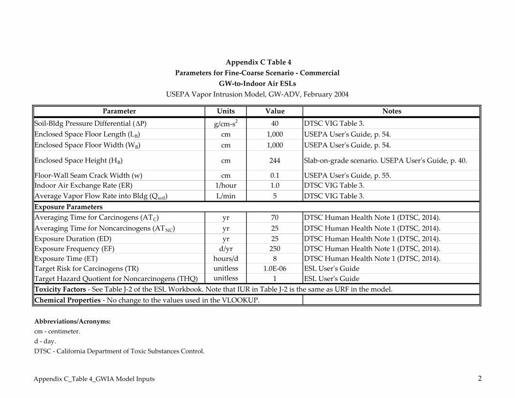
Appendix C Table 4Parameters for Fine‐Coarse Scenario ‐ Commercial
GW‐to‐Indoor Air ESLsUSEPA Vapor Intrusion Model, GW‐ADV, February 2004
Parameter Units Value Notes
Soil‐Bldg Pressure Differential (ΔΡ) g/cm‐s2 40 DTSC VIG Table 3.
Enclosed Space Floor Length (LB) cm 1,000 USEPA Userʹs Guide, p. 54.
Enclosed Space Floor Width (WB) cm 1,000 USEPA Userʹs Guide, p. 54.
Enclosed Space Height (HB) cm 244 Slab‐on‐grade scenario. USEPA Userʹs Guide, p. 40.
Floor‐Wall Seam Crack Width (w) cm 0.1 USEPA Userʹs Guide, p. 55.
Indoor Air Exchange Rate (ER) 1/hour 1.0 DTSC VIG Table 3.
Average Vapor Flow Rate into Bldg (Qsoil) L/min 5 DTSC VIG Table 3.
Exposure ParametersAveraging Time for Carcinogens (ATC) yr 70 DTSC Human Health Note 1 (DTSC, 2014).
Averaging Time for Noncarcinogens (ATNC) yr 25 DTSC Human Health Note 1 (DTSC, 2014).
Exposure Duration (ED) yr 25 DTSC Human Health Note 1 (DTSC, 2014).
Exposure Frequency (EF) d/yr 250 DTSC Human Health Note 1 (DTSC, 2014).
Exposure Time (ET) hours/d 8 DTSC Human Health Note 1 (DTSC, 2014).
Target Risk for Carcinogens (TR) unitless 1.0E‐06 ESL Userʹs Guide
Target Hazard Quotient for Noncarcinogens (THQ) unitless 1 ESL Userʹs Guide
Toxicity Factors ‐ See Table J‐2 of the ESL Workbook. Note that IUR in Table J‐2 is the same as URF in the model.
Chemical Properties ‐ No change to the values used in the VLOOKUP.
Abbreviations/Acronyms:cm ‐ centimeter.
d ‐ day.
DTSC ‐ California Department of Toxic Substances Control.
Appendix C_Table 4_GWIA Model Inputs 2

Appendix C Table 4Parameters for Fine‐Coarse Scenario ‐ Commercial
GW‐to‐Indoor Air ESLsUSEPA Vapor Intrusion Model, GW‐ADV, February 2004
Parameter Units Value NotesDTSC VIG ‐ Guidance for the Evaluation and Mitigation of Subsurface Vapor Intrusion to Indoor Air (Vapor Intrusion Guidance) (DTSC, 2011).
g ‐ gram.
L ‐ liter.
min ‐ minute.
s ‐ second.
SCS ‐ Soil Conservation Service; now the Natural Resources Conservation Service (NRCS).
U.S. DA ‐ United States Department of Agriculture.
USEPA ‐ United States Environmental Protection Agency.
USEPA Userʹs Guide ‐ User’s Guide for Evaluating Subsurface Vapor Intrusion into Buildings (Environmental Quality Management 2004).
yr ‐ year.
Note:
References:DTSC. 2014. Human Health Risk Assessment Health Note 1. Office of Human and Ecological Risk (HERO). September 30
DTSC. 2011. Final Guidance for the Evaluation and Mitigation of Subsurface Vapor Intrusion to Indoor Air (Vapor Intrusion Guidance). October.
Emergency Response. May.
(1) USDA SCS ‐ The USDA SCS Soil Texture Classification system employed in the USEPA Vapor Intrusion Model differs from the Unified Soil
Classification System (USCS), which is the system commonly used for soil logging in the environmental remediation industry. See the USEPA Userʹs
Guide for further information.
USEPA. 1996. Soil Screening Guidance: Technical Background Document. EPA‐540‐R95‐128. Washington, D.C. Office of Solid Waste and
Environmental Quality Management. 2004. User’s Guide for Evaluating Subsurface Vapor Intrusion into Buildings. Prepared for
U.S. Environmental Protection Agency Office of Emergency and Remedial Response. February 22.
Appendix C_Table 4_GWIA Model Inputs 3

Scenario: ResidentialChemical: Tetrachloroethylene
YES XOR
YESSoil Gas Conc. Attenuation Factor Indoor Air Conc. Cancer Noncancer Cancer Risk Noncancer
ENTER ENTER (Csource) (alpha) (Cbuilding) Risk Hazard = 10-6 HQ = 1Initial (µg/m3) (unitless) (µg/m3) (μg/L) (μg/L)
Chemical groundwater 4.29E+02 3.7E‐04 1.6E‐01 NA NA 3.0E+00 2.3E+02CAS No. conc., MESSAGE: Values of Csource and Cbuilding (INTERCALCS worksheet) are based on unity and do not represent actual values.
(numbers only, CWno dashes) (µg/L)
127184 Tetrachloroethylene
ENTER ENTER ENTER ENTERMORE Depth below grade Average ENTER
to bottom Depth soil/ Average vaporof enclosed below grade SCS groundwater flow rate into bldg.space floor, to water table, soil type temperature, (Leave blank to calculate)
LF LWT directly above TS Qsoil
(15 or 200 cm) (cm) water table (oC) (L/m)
15 152 S 15 5
MORE
ENTER ENTERVadose zone User-defined ENTER ENTER ENTER ENTER
SCS vandose zone Vadose zone Vadose zone Vadose zone Vadose zonesoil type soil vapor SCS soil dry soil total soil water-filled
(used to estimate OR permeability, soil type bulk density, porosity, porosity,soil vapor kv b
V nV wV
permeability) (cm2) (g/cm3) (unitless) (cm3/cm3)
S S 1.66 0.375 0.054
MORE ENTER ENTER ENTER ENTER ENTER ENTER ENTER ENTER
Target Target hazard Averaging Averagingrisk for quotient for time for time for Exposure Exposure Exposure Air Exchange
carcinogens, noncarcinogens, carcinogens, noncarcinogens, duration, frequency, Time RateTR THQ ATC ATNC ED EF ET ACH
(unitless) (unitless) (yrs) (yrs) (yrs) (days/yr) (hrs/day) (hour)-1
Residential 1.0E-06 1 70 26 26 350 24 0.5Used to calculate risk-basedgroundwater concentration.
END
USEPA GW-SCREEN Version 3.0, 04/2003
DTSC Modification December 2014
Risk-Based Groundwater Concentration
DATA ENTRY SHEET
CALCULATE INCREMENTAL RISKS FROM ACTUAL GROUNDWATER CONCENTRATION(enter "X" in "YES" box and initial groundwater conc. below)
Results Summary
Chemical
Groundwater to Indoor Air ESL - Shallow Groundwater, Sand Scenario
CALCULATE RISK-BASED GROUNDWATER CONCENTRATION (enter "X" in "YES" box)
Reset to Defaults
Lookup Soil Parameters
Lookup Receptor Parameters
Last Update: December 2014DTSC Human and Ecological Risk Office GWIA ESL_Shallow GW_Sand_Res_PCE
DATENTERPage 1 of 1

CHEMICAL PROPERTIES SHEET
Tetrachloroethylene
Henry's Henry's Enthalpy of Organic Purelaw constant law constant vaporization at Normal carbon component Unit
Diffusivity Diffusivity at reference reference the normal boiling Critical partition water risk Referencein air, in water, temperature, temperature, boiling point, point, temperature, coefficient, solubility, factor, conc.,
Da Dw H TR Hv,b TB TC Koc S URF RfC(cm2/s) (cm2/s) (atm-m3/mol) (oC) (cal/mol) (oK) (oK) (cm3/g) (mg/L) (g/m3)-1 (mg/m3)
5.05E-02 9.46E-06 1.77E-02 25 8,288 394.40 620.20 9.49E+01 2.06E+02 5.9E-06 3.5E-02
END
Last Update: December 2014DTSC Human and Ecological Risk Office GWIA ESL_Shallow GW_Sand_Res_PCE
CHEMPROPSPage 1 of 1

INTERMEDIATE CALCULATIONS SHEET
Scenario: Residential
Chemical:
Vadose Vadose zone Vadose zone Vadose zone Vadose zone Total Air-filled Water-filled Floor-Source- zone soil effective soil soil soil Thickness of porosity in porosity in porosity in wallbuilding air-filled total fluid intrinsic relative air effective vapor capillary capillary capillary capillary seam
separation, porosity, saturation, permeability, permeability, permeability, zone, zone, zone, zone, perimeter,LT a
V Ste ki krg kv Lcz ncz a,cz w,cz Xcrack
(cm) (cm3/cm3) (cm3/cm3) (cm2) (cm2) (cm2) (cm) (cm3/cm3) (cm3/cm3) (cm3/cm3) (cm)
137 0.321 0.003 1.00E-07 0.998 9.99E-08 17.05 0.375 0.122 0.253 4,000
Area of Capillary Totalenclosed Crack- Crack Enthalpy of Henry's law Henry's law Vapor Vadose zone zone overall
Bldg. space to-total depth vaporization at constant at constant at viscosity at effective effective effectiveventilation below area below ave. groundwater ave. groundwater ave. groundwater ave. soil diffusion diffusion diffusion
rate, grade, ratio, grade, temperature, temperature, temperature, temperature, coefficient, coefficient, coefficient,Qbuilding AB Zcrack Hv,TS HTS H'TS TS Deff
V Deffcz Deff
T
(cm3/s) (cm2) (unitless) (cm) (cal/mol) (atm-m3/mol) (unitless) (g/cm-s) (cm2/s) (cm2/s) (cm2/s)
3.39E+04 1.00E+06 5.00E-03 15 9,502 1.01E-02 4.29E-01 1.77E-04 8.16E-03 3.25E-04 2.04E-03
Exponent of InfiniteAverage Crack equivalent source Infinite
Diffusion Convection Source vapor effective foundation indoor source Unitpath path vapor Crack flow rate diffusion Area of Peclet attenuation bldg. risk Reference
length, length, conc., radius, into bldg., coefficient, crack, number, coefficient, conc., factor, conc.,Ld Lp Csource rcrack Qsoil Dcrack Acrack exp(Pef) Cbuilding URF RfC
(cm) (cm) (g/m3) (cm) (cm3/s) (cm2/s) (cm2) (unitless) (unitless) (g/m3) (g/m3)-1 (mg/m3)
137 15 4.29E+02 1.25 8.33E+01 8.16E-03 5.00E+03 7.45E+08 3.73E-04 1.60E-01 5.9E-06 3.5E-02
END
Tetrachloroethylene
Last Update: December 2014DTSC Human and Ecological Risk Office GWIA ESL_Shallow GW_Sand_Res_PCE
INTERCALCSPage 1 of 1

RESULTS SHEET
Scenario: ResidentialChemical:
RISK-BASED GROUNDWATER CONCENTRATION CALCULATIONS: INCREMENTAL RISK CALCULATIONS:
Incremental HazardIndoor Indoor Risk-based Pure Final risk from quotient
exposure exposure indoor component indoor vapor from vaporgroundwater groundwater exposure water exposure intrusion to intrusion to
conc., conc., groundwater solubility, groundwater indoor air, indoor air,carcinogen noncarcinogen conc., S conc., carcinogen noncarcinogen
(g/L) (g/L) (g/L) (g/L) (g/L) (unitless) (unitless)
2.98E+00 2.28E+02 2.98E+00 2.06E+05 2.98E+00 NA NA
MESSAGE SUMMARY BELOW:MESSAGE: Values of Csource and Cbuilding (INTERCALCS worksheet) are based on unity and do not represent actual values.
END
Tetrachloroethylene
Last Update:December 2014DTSC Human and Ecological Risk Office GWIA ESL_Shallow GW_Sand_Res_PCE
RESULTSPage 1 of 1

Scenario: CommercialChemical: Trichloroethylene
YES X
OR
YES
Soil Gas Conc. Attenuation Factor Indoor Air Conc. Cancer Noncancer Cancer Risk Noncancer
ENTER ENTER (Csource) (alpha) (Cbuilding) Risk Hazard = 10-6 HQ = 1Initial (µg/m3) (unitless) (µg/m3) (μg/L) (μg/L)
Chemical groundwater 2.53E+02 2.4E‐04 6.1E‐02 NA NA 4.9E+01 1.4E+02CAS No. conc., MESSAGE: Values of Csource and Cbuilding (INTERCALCS worksheet) are based on unity and do not represent actual values.
(numbers only, CW
no dashes) (µg/L)
79016 Trichloroethylene
ENTER ENTER ENTER ENTERMORE Depth below grade Average ENTER
to bottom Depth soil/ Average vaporof enclosed below grade SCS groundwater flow rate into bldg.space floor, to water table, soil type temperature, (Leave blank to calculate)
LF LWT directly above TS Qsoil
(15 or 200 cm) (cm) water table (oC) (L/m)
15 152 S 15 5
MORE
ENTER ENTERVadose zone User-defined ENTER ENTER ENTER ENTER
SCS vandose zone Vadose zone Vadose zone Vadose zone Vadose zonesoil type soil vapor SCS soil dry soil total soil water-filled
(used to estimate OR permeability, soil type bulk density, porosity, porosity,
soil vapor kv bV nV w
V
permeability) (cm2) (g/cm3) (unitless) (cm3/cm3)
S S 1.66 0.375 0.054
MORE ENTER ENTER ENTER ENTER ENTER ENTER ENTER ENTER
Target Target hazard Averaging Averagingrisk for quotient for time for time for Exposure Exposure Exposure Air Exchange
carcinogens, noncarcinogens, carcinogens, noncarcinogens, duration, frequency, Time RateTR THQ ATC ATNC ED EF ET ACH
(unitless) (unitless) (yrs) (yrs) (yrs) (days/yr) (hrs/day) (hour)-1
Commercial 1.0E-06 1 70 25 25 250 8 1Used to calculate risk-based
groundwater concentration.
END
MESSAGE: See VLOOKUP table comments on chemical properties and/or toxicity criteria for this chemical.
Results Summary
Chemical
Groundwater to Indoor Air ESL - Shallow Groundwater, Sand Scenario
CALCULATE RISK-BASED GROUNDWATER CONCENTRATION (enter "X" in "YES" box)
USEPA GW-SCREEN Version 3.0, 04/2003
DTSC Modification December 2014
Risk-Based Groundwater Concentration
DATA ENTRY SHEET
CALCULATE INCREMENTAL RISKS FROM ACTUAL GROUNDWATER CONCENTRATION
(enter "X" in "YES" box and initial groundwater conc. below)
Reset to Defaults
Lookup Soil Parameters
Lookup Receptor Parameters
Last Update: December 2014DTSC Human and Ecological Risk Office GWIA ESL_Sand_Com_PCE
DATENTERPage 1 of 1

CHEMICAL PROPERTIES SHEET
Trichloroethylene
Henry's Henry's Enthalpy of Organic Purelaw constant law constant vaporization at Normal carbon component Unit
Diffusivity Diffusivity at reference reference the normal boiling Critical partition water risk Referencein air, in water, temperature, temperature, boiling point, point, temperature, coefficient, solubility, factor, conc.,
Da Dw H TR Hv,b TB TC Koc S URF RfC(cm2/s) (cm2/s) (atm-m3/mol) (oC) (cal/mol) (oK) (oK) (cm3/g) (mg/L) (g/m3)-1 (mg/m3)
6.87E-02 1.02E-05 9.85E-03 25 7,505 360.36 544.20 6.07E+01 1.28E+03 4.1E-06 2.0E-03
END
Last Update: December 2014DTSC Human and Ecological Risk Office GWIA ESL_Sand_Com_PCE
CHEMPROPSPage 1 of 1

INTERMEDIATE CALCULATIONS SHEET
Scenario: Commercial
Chemical:
Vadose Vadose zone Vadose zone Vadose zone Vadose zone Total Air-filled Water-filled Floor-Source- zone soil effective soil soil soil Thickness of porosity in porosity in porosity in wallbuilding air-filled total fluid intrinsic relative air effective vapor capillary capillary capillary capillary seam
separation, porosity, saturation, permeability, permeability, permeability, zone, zone, zone, zone, perimeter,LT a
V Ste ki krg kv Lcz ncz a,cz w,cz Xcrack
(cm) (cm3/cm3) (cm3/cm3) (cm2) (cm2) (cm2) (cm) (cm3/cm3) (cm3/cm3) (cm3/cm3) (cm)
137 0.321 0.003 1.00E-07 0.998 9.99E-08 17.05 0.375 0.122 0.253 4,000
Area of Capillary Totalenclosed Crack- Crack Enthalpy of Henry's law Henry's law Vapor Vadose zone zone overall
Bldg. space to-total depth vaporization at constant at constant at viscosity at effective effective effectiveventilation below area below ave. groundwater ave. groundwater ave. groundwater ave. soil diffusion diffusion diffusion
rate, grade, ratio, grade, temperature, temperature, temperature, temperature, coefficient, coefficient, coefficient,Qbuilding AB Zcrack Hv,TS HTS H'TS TS Deff
V Deffcz Deff
T
(cm3/s) (cm2) (unitless) (cm) (cal/mol) (atm-m3/mol) (unitless) (g/cm-s) (cm2/s) (cm2/s) (cm2/s)
6.78E+04 1.00E+06 5.00E-03 15 8,495 5.99E-03 2.53E-01 1.77E-04 1.11E-02 4.43E-04 2.78E-03
Exponent of InfiniteAverage Crack equivalent source Infinite
Diffusion Convection Source vapor effective foundation indoor source Unitpath path vapor Crack flow rate diffusion Area of Peclet attenuation bldg. risk Reference
length, length, conc., radius, into bldg., coefficient, crack, number, coefficient, conc., factor, conc.,Ld Lp Csource rcrack Qsoil Dcrack Acrack exp(Pef) Cbuilding URF RfC
(cm) (cm) (g/m3) (cm) (cm3/s) (cm2/s) (cm2) (unitless) (unitless) (g/m3) (g/m3)-1 (mg/m3)
137 15 2.53E+02 1.25 8.33E+01 1.11E-02 5.00E+03 3.32E+06 2.41E-04 6.09E-02 4.1E-06 2.0E-03
END
Trichloroethylene
Last Update: December 2014DTSC Human and Ecological Risk Office GWIA ESL_Sand_Com_PCE
INTERCALCSPage 1 of 1

RESULTS SHEET
Scenario: CommercialChemical:
RISK-BASED GROUNDWATER CONCENTRATION CALCULATIONS: INCREMENTAL RISK CALCULATIONS:
Incremental HazardIndoor Indoor Risk-based Pure Final risk from quotient
exposure exposure indoor component indoor vapor from vaporgroundwater groundwater exposure water exposure intrusion to intrusion to
conc., conc., groundwater solubility, groundwater indoor air, indoor air,carcinogen noncarcinogen conc., S conc., carcinogen noncarcinogen
(g/L) (g/L) (g/L) (g/L) (g/L) (unitless) (unitless)
4.91E+01 1.44E+02 4.91E+01 1.28E+06 4.91E+01 NA NA
MESSAGE SUMMARY BELOW:MESSAGE: Values of Csource and Cbuilding (INTERCALCS worksheet) are based on unity and do not represent actual values.
END
Trichloroethylene
Last Update:December 2014DTSC Human and Ecological Risk Office GWIA ESL_Sand_Com_PCE
RESULTSPage 1 of 1

Scenario: ResidentialChemical: Tetrachloroethylene
YES XOR
YESSoil Gas Conc. Attenuation Factor Indoor Air Conc. Cancer Noncancer Cancer Risk Noncancer
ENTER ENTER (Csource) (alpha) (Cbuilding) Risk Hazard = 10-6 HQ = 1Initial (µg/m3) (unitless) (µg/m3) (μg/L) (μg/L)
Chemical groundwater 4.29E+02 3.0E‐04 1.3E‐01 NA NA 3.7E+00 2.8E+02CAS No. conc., MESSAGE: Values of Csource and Cbuilding (INTERCALCS worksheet) are based on unity and do not represent actual values.
(numbers only, CWno dashes) (µg/L)
127184 Tetrachloroethylene
ENTER ENTER ENTER ENTERMORE Depth below grade Average ENTER
to bottom Depth soil/ Average vaporof enclosed below grade SCS groundwater flow rate into bldg.space floor, to water table, soil type temperature, (Leave blank to calculate)
LF LWT directly above TS Qsoil
(15 or 200 cm) (cm) water table (oC) (L/m)
15 304 S 15 5
MORE
ENTER ENTERVadose zone User-defined ENTER ENTER ENTER ENTER
SCS vandose zone Vadose zone Vadose zone Vadose zone Vadose zonesoil type soil vapor SCS soil dry soil total soil water-filled
(used to estimate OR permeability, soil type bulk density, porosity, porosity,soil vapor kv b
V nV wV
permeability) (cm2) (g/cm3) (unitless) (cm3/cm3)
S S 1.66 0.375 0.054
MORE ENTER ENTER ENTER ENTER ENTER ENTER ENTER ENTER
Target Target hazard Averaging Averagingrisk for quotient for time for time for Exposure Exposure Exposure Air Exchange
carcinogens, noncarcinogens, carcinogens, noncarcinogens, duration, frequency, Time RateTR THQ ATC ATNC ED EF ET ACH
(unitless) (unitless) (yrs) (yrs) (yrs) (days/yr) (hrs/day) (hour)-1
Residential 1.0E-06 1 70 26 26 350 24 0.5Used to calculate risk-basedgroundwater concentration.
END
USEPA GW-SCREEN Version 3.0, 04/2003
DTSC Modification December 2014
Risk-Based Groundwater Concentration
DATA ENTRY SHEET
CALCULATE INCREMENTAL RISKS FROM ACTUAL GROUNDWATER CONCENTRATION(enter "X" in "YES" box and initial groundwater conc. below)
Results Summary
Chemical
Groundwater to Indoor Air ESL - Deep Groundwater, Sand Scenario
CALCULATE RISK-BASED GROUNDWATER CONCENTRATION (enter "X" in "YES" box)
Reset to Defaults
Lookup Soil Parameters
Lookup Receptor Parameters
Last Update: December 2014DTSC Human and Ecological Risk Office GWIA ESL_Deep GW_Sand_Res_PCE
DATENTERPage 1 of 1

CHEMICAL PROPERTIES SHEET
Tetrachloroethylene
Henry's Henry's Enthalpy of Organic Purelaw constant law constant vaporization at Normal carbon component Unit
Diffusivity Diffusivity at reference reference the normal boiling Critical partition water risk Referencein air, in water, temperature, temperature, boiling point, point, temperature, coefficient, solubility, factor, conc.,
Da Dw H TR Hv,b TB TC Koc S URF RfC(cm2/s) (cm2/s) (atm-m3/mol) (oC) (cal/mol) (oK) (oK) (cm3/g) (mg/L) (g/m3)-1 (mg/m3)
5.05E-02 9.46E-06 1.77E-02 25 8,288 394.40 620.20 9.49E+01 2.06E+02 5.9E-06 3.5E-02
END
Last Update: December 2014DTSC Human and Ecological Risk Office GWIA ESL_Deep GW_Sand_Res_PCE
CHEMPROPSPage 1 of 1

INTERMEDIATE CALCULATIONS SHEET
Scenario: Residential
Chemical:
Vadose Vadose zone Vadose zone Vadose zone Vadose zone Total Air-filled Water-filled Floor-Source- zone soil effective soil soil soil Thickness of porosity in porosity in porosity in wallbuilding air-filled total fluid intrinsic relative air effective vapor capillary capillary capillary capillary seam
separation, porosity, saturation, permeability, permeability, permeability, zone, zone, zone, zone, perimeter,LT a
V Ste ki krg kv Lcz ncz a,cz w,cz Xcrack
(cm) (cm3/cm3) (cm3/cm3) (cm2) (cm2) (cm2) (cm) (cm3/cm3) (cm3/cm3) (cm3/cm3) (cm)
289 0.321 0.003 1.00E-07 0.998 9.99E-08 17.05 0.375 0.122 0.253 4,000
Area of Capillary Totalenclosed Crack- Crack Enthalpy of Henry's law Henry's law Vapor Vadose zone zone overall
Bldg. space to-total depth vaporization at constant at constant at viscosity at effective effective effectiveventilation below area below ave. groundwater ave. groundwater ave. groundwater ave. soil diffusion diffusion diffusion
rate, grade, ratio, grade, temperature, temperature, temperature, temperature, coefficient, coefficient, coefficient,Qbuilding AB Zcrack Hv,TS HTS H'TS TS Deff
V Deffcz Deff
T
(cm3/s) (cm2) (unitless) (cm) (cal/mol) (atm-m3/mol) (unitless) (g/cm-s) (cm2/s) (cm2/s) (cm2/s)
3.39E+04 1.00E+06 5.00E-03 15 9,502 1.01E-02 4.29E-01 1.77E-04 8.16E-03 3.25E-04 3.37E-03
Exponent of InfiniteAverage Crack equivalent source Infinite
Diffusion Convection Source vapor effective foundation indoor source Unitpath path vapor Crack flow rate diffusion Area of Peclet attenuation bldg. risk Reference
length, length, conc., radius, into bldg., coefficient, crack, number, coefficient, conc., factor, conc.,Ld Lp Csource rcrack Qsoil Dcrack Acrack exp(Pef) Cbuilding URF RfC
(cm) (cm) (g/m3) (cm) (cm3/s) (cm2/s) (cm2) (unitless) (unitless) (g/m3) (g/m3)-1 (mg/m3)
289 15 4.29E+02 1.25 8.33E+01 8.16E-03 5.00E+03 7.45E+08 3.02E-04 1.29E-01 5.9E-06 3.5E-02
END
Tetrachloroethylene
Last Update: December 2014DTSC Human and Ecological Risk Office GWIA ESL_Deep GW_Sand_Res_PCE
INTERCALCSPage 1 of 1

RESULTS SHEET
Scenario: ResidentialChemical:
RISK-BASED GROUNDWATER CONCENTRATION CALCULATIONS: INCREMENTAL RISK CALCULATIONS:
Incremental HazardIndoor Indoor Risk-based Pure Final risk from quotient
exposure exposure indoor component indoor vapor from vaporgroundwater groundwater exposure water exposure intrusion to intrusion to
conc., conc., groundwater solubility, groundwater indoor air, indoor air,carcinogen noncarcinogen conc., S conc., carcinogen noncarcinogen
(g/L) (g/L) (g/L) (g/L) (g/L) (unitless) (unitless)
3.68E+00 2.82E+02 3.68E+00 2.06E+05 3.68E+00 NA NA
MESSAGE SUMMARY BELOW:MESSAGE: Values of Csource and Cbuilding (INTERCALCS worksheet) are based on unity and do not represent actual values.
END
Tetrachloroethylene
Last Update:December 2014DTSC Human and Ecological Risk Office GWIA ESL_Deep GW_Sand_Res_PCE
RESULTSPage 1 of 1
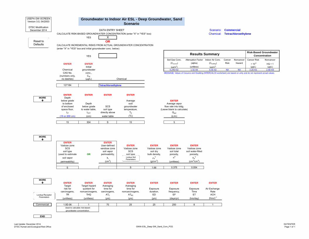
Scenario: CommercialChemical: Tetrachloroethylene
YES XOR
YESSoil Gas Conc. Attenuation Factor Indoor Air Conc. Cancer Noncancer Cancer Risk Noncancer
ENTER ENTER (Csource) (alpha) (Cbuilding) Risk Hazard = 10-6 HQ = 1Initial (µg/m3) (unitless) (µg/m3) (μg/L) (μg/L)
Chemical groundwater 4.29E+02 1.5E‐04 6.5E‐02 NA NA 3.2E+01 2.4E+03CAS No. conc., MESSAGE: Values of Csource and Cbuilding (INTERCALCS worksheet) are based on unity and do not represent actual values.
(numbers only, CWno dashes) (µg/L)
127184 Tetrachloroethylene
ENTER ENTER ENTER ENTERMORE Depth below grade Average ENTER
to bottom Depth soil/ Average vaporof enclosed below grade SCS groundwater flow rate into bldg.space floor, to water table, soil type temperature, (Leave blank to calculate)
LF LWT directly above TS Qsoil
(15 or 200 cm) (cm) water table (oC) (L/m)
15 304 S 15 5
MORE
ENTER ENTERVadose zone User-defined ENTER ENTER ENTER ENTER
SCS vandose zone Vadose zone Vadose zone Vadose zone Vadose zonesoil type soil vapor SCS soil dry soil total soil water-filled
(used to estimate OR permeability, soil type bulk density, porosity, porosity,soil vapor kv b
V nV wV
permeability) (cm2) (g/cm3) (unitless) (cm3/cm3)
S S 1.66 0.375 0.054
MORE ENTER ENTER ENTER ENTER ENTER ENTER ENTER ENTER
Target Target hazard Averaging Averagingrisk for quotient for time for time for Exposure Exposure Exposure Air Exchange
carcinogens, noncarcinogens, carcinogens, noncarcinogens, duration, frequency, Time RateTR THQ ATC ATNC ED EF ET ACH
(unitless) (unitless) (yrs) (yrs) (yrs) (days/yr) (hrs/day) (hour)-1
Commercial 1.0E-06 1 70 25 25 250 8 1Used to calculate risk-basedgroundwater concentration.
END
Results Summary
Chemical
Groundwater to Indoor Air ESL - Deep Groundwater, Sand Scenario
CALCULATE RISK-BASED GROUNDWATER CONCENTRATION (enter "X" in "YES" box)
USEPA GW-SCREEN Version 3.0, 04/2003
DTSC Modification December 2014
Risk-Based Groundwater Concentration
DATA ENTRY SHEET
CALCULATE INCREMENTAL RISKS FROM ACTUAL GROUNDWATER CONCENTRATION(enter "X" in "YES" box and initial groundwater conc. below)
Reset to Defaults
Lookup Soil Parameters
Lookup Receptor Parameters
Last Update: December 2014DTSC Human and Ecological Risk Office GWIA ESL_Deep GW_Sand_Com_PCE
DATENTERPage 1 of 1

CHEMICAL PROPERTIES SHEET
Tetrachloroethylene
Henry's Henry's Enthalpy of Organic Purelaw constant law constant vaporization at Normal carbon component Unit
Diffusivity Diffusivity at reference reference the normal boiling Critical partition water risk Referencein air, in water, temperature, temperature, boiling point, point, temperature, coefficient, solubility, factor, conc.,
Da Dw H TR Hv,b TB TC Koc S URF RfC(cm2/s) (cm2/s) (atm-m3/mol) (oC) (cal/mol) (oK) (oK) (cm3/g) (mg/L) (g/m3)-1 (mg/m3)
5.05E-02 9.46E-06 1.77E-02 25 8,288 394.40 620.20 9.49E+01 2.06E+02 5.9E-06 3.5E-02
END
Last Update: December 2014DTSC Human and Ecological Risk Office GWIA ESL_Deep GW_Sand_Com_PCE
CHEMPROPSPage 1 of 1
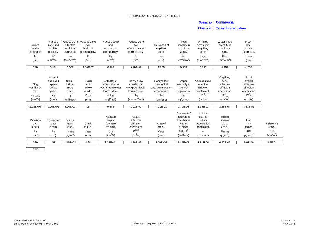
INTERMEDIATE CALCULATIONS SHEET
Scenario: Commercial
Chemical:
Vadose Vadose zone Vadose zone Vadose zone Vadose zone Total Air-filled Water-filled Floor-Source- zone soil effective soil soil soil Thickness of porosity in porosity in porosity in wallbuilding air-filled total fluid intrinsic relative air effective vapor capillary capillary capillary capillary seam
separation, porosity, saturation, permeability, permeability, permeability, zone, zone, zone, zone, perimeter,LT a
V Ste ki krg kv Lcz ncz a,cz w,cz Xcrack
(cm) (cm3/cm3) (cm3/cm3) (cm2) (cm2) (cm2) (cm) (cm3/cm3) (cm3/cm3) (cm3/cm3) (cm)
289 0.321 0.003 1.00E-07 0.998 9.99E-08 17.05 0.375 0.122 0.253 4,000
Area of Capillary Totalenclosed Crack- Crack Enthalpy of Henry's law Henry's law Vapor Vadose zone zone overall
Bldg. space to-total depth vaporization at constant at constant at viscosity at effective effective effectiveventilation below area below ave. groundwater ave. groundwater ave. groundwater ave. soil diffusion diffusion diffusion
rate, grade, ratio, grade, temperature, temperature, temperature, temperature, coefficient, coefficient, coefficient,Qbuilding AB Zcrack Hv,TS HTS H'TS TS Deff
V Deffcz Deff
T
(cm3/s) (cm2) (unitless) (cm) (cal/mol) (atm-m3/mol) (unitless) (g/cm-s) (cm2/s) (cm2/s) (cm2/s)
6.78E+04 1.00E+06 5.00E-03 15 9,502 1.01E-02 4.29E-01 1.77E-04 8.16E-03 3.25E-04 3.37E-03
Exponent of InfiniteAverage Crack equivalent source Infinite
Diffusion Convection Source vapor effective foundation indoor source Unitpath path vapor Crack flow rate diffusion Area of Peclet attenuation bldg. risk Reference
length, length, conc., radius, into bldg., coefficient, crack, number, coefficient, conc., factor, conc.,Ld Lp Csource rcrack Qsoil Dcrack Acrack exp(Pef) Cbuilding URF RfC
(cm) (cm) (g/m3) (cm) (cm3/s) (cm2/s) (cm2) (unitless) (unitless) (g/m3) (g/m3)-1 (mg/m3)
289 15 4.29E+02 1.25 8.33E+01 8.16E-03 5.00E+03 7.45E+08 1.51E-04 6.47E-02 5.9E-06 3.5E-02
END
Tetrachloroethylene
Last Update: December 2014DTSC Human and Ecological Risk Office GWIA ESL_Deep GW_Sand_Com_PCE
INTERCALCSPage 1 of 1

RESULTS SHEET
Scenario: CommercialChemical:
RISK-BASED GROUNDWATER CONCENTRATION CALCULATIONS: INCREMENTAL RISK CALCULATIONS:
Incremental HazardIndoor Indoor Risk-based Pure Final risk from quotient
exposure exposure indoor component indoor vapor from vaporgroundwater groundwater exposure water exposure intrusion to intrusion to
conc., conc., groundwater solubility, groundwater indoor air, indoor air,carcinogen noncarcinogen conc., S conc., carcinogen noncarcinogen
(g/L) (g/L) (g/L) (g/L) (g/L) (unitless) (unitless)
3.21E+01 2.37E+03 3.21E+01 2.06E+05 3.21E+01 NA NA
MESSAGE SUMMARY BELOW:MESSAGE: Values of Csource and Cbuilding (INTERCALCS worksheet) are based on unity and do not represent actual values.
END
Tetrachloroethylene
Last Update:December 2014DTSC Human and Ecological Risk Office GWIA ESL_Deep GW_Sand_Com_PCE
RESULTSPage 1 of 1

DATA ENTRY SHEET
CALCULATE RISK-BASED GROUNDWATER CONCENTRATION (enter "X" in "YES" box)
YES XOR
CALCULATE INCREMENTAL RISKS FROM ACTUAL GROUNDWATER CONCENTRATION (enter "X" in "YES" box and initial groundwater conc. below)
YES San Francisco Bay Regional Water Quality Control BoardSoil Layer Design: Fine-Coarse Scenario
ENTER ENTER Exposure Scenario: ResidentialInitial Cancer Risk GW (µg/L): 1.0E+02
Chemical groundwater Noncancer Hazard GW (µg/L): 7.7E+03CAS No. conc., GW ESL (µg/L): 1.0E+02
(numbers only, CW
no dashes) (g/L) Chemical
127184 Tetrachloroethylene
ENTER ENTER ENTER ENTER ENTER ENTER ENTER ENTER ENTER ENTERDepth Totals must add up to value of LWT (cell G28) Soil
MORE Average below grade Thickness Thickness stratum A User-defined soil/ to bottom Depth Thickness of soil of soil Soil SCS stratum A
groundwater of enclosed below grade of soil stratum B, stratum C, stratum SCS soil type soil vaportemperature, space floor, to water table, stratum A, (Enter value or 0) (Enter value or 0) directly above soil type (used to estimate OR permeability,
TS LF LWT hA hB hC water table, directly above soil vapor kv
(oC) (cm) (cm) (cm) (cm) (cm) (Enter A, B, or C) water table permeability) (cm2)
15 15 300 100 200 B CL S
ENTER ENTER ENTER ENTER ENTER ENTER ENTER ENTER ENTER ENTER ENTER ENTERMORE Stratum A Stratum A Stratum A Stratum A Stratum B Stratum B Stratum B Stratum B Stratum C Stratum C Stratum C Stratum C SCS soil dry soil total soil water-filled SCS soil dry soil total soil water-filled SCS soil dry soil total soil water-filled
soil type bulk density, porosity, porosity, soil type bulk density, porosity, porosity, soil type bulk density, porosity, porosity,b
A nA wA b
B nB wB b
C nC wC
(g/cm3) (unitless) (cm3/cm3) (g/cm3) (unitless) (cm3/cm3) (g/cm3) (unitless) (cm3/cm3)
S 1.50 0.430 0.15 CL 1.5 0.43 0.3
ENTER ENTER ENTER ENTER ENTER ENTER ENTER ENTERMORE Enclosed Enclosed Enclosed Average vapor space Soil-bldg. space space Enclosed Floor-wall Indoor flow rate into bldg.
floor pressure floor floor space seam crack air exchange ORthickness, differential, length, width, height, width, rate, Leave blank to calculate
Lcrack P LB WB HB w ER Qsoil
(cm) (g/cm-s2) (cm) (cm) (cm) (cm) (1/h) (L/m)
15 40 1000 1000 244 0.1 0.5 5
MORE ENTER ENTER ENTER ENTER ENTER ENTER ENTER Averaging Averaging Target Target hazard
time for time for Exposure Exposure Exposure risk for quotient forcarcinogens, noncarcinogens, duration, frequency, time, carcinogens, noncarcinogens,
ATC ATNC ED EF ET TR THQ(yrs) (yrs) (yrs) (days/yr) (hours/day) (unitless) (unitless)
70 26 26 350 24 1.0E-06 1.0
Used to calculate risk-basedEND groundwater concentration.
GW-ADVVersion 3.1; 02/04Re
Lookup Soil Parameters
Lookup Soil Parameters
Lookup Soil Parameters
GW-ADV-Dec15_FC_Res_PCE 1 of 1

CHEMICAL PROPERTIES SHEET
Henry's Henry's Enthalpy of Organic Purelaw constant law constant vaporization at Normal carbon component Unit
Diffusivity Diffusivity at reference reference the normal boiling Critical partition water risk Referencein air, in water, temperature, temperature, boiling point, point, temperature, coefficient, solubility, factor, conc.,
Da Dw H TR Hv,b TB TC Koc S URF RfC(cm2/s) (cm2/s) (atm-m3/mol) (oC) (cal/mol) (oK) (oK) (cm3/g) (mg/L) (g/m3)-1 (mg/m3)
5.05E-02 9.46E-06 1.77E-02 25 8,288 394.40 620.20 9.49E+01 2.06E+02 5.9E-06 3.5E-02
END
GW-ADV-Dec15_FC_Res_PCE 1 of 1

INTERMEDIATE CALCULATIONS SHEET
Stratum A Stratum B Stratum C Stratum A Stratum A Stratum A Stratum A Total Air-filled Water-filled Floor-Source- soil soil soil effective soil soil soil Thickness of porosity in porosity in porosity in wall
Exposure building air-filled air-filled air-filled total fluid intrinsic relative air effective vapor capillary capillary capillary capillary seamduration, separation, porosity, porosity, porosity, saturation, permeability, permeability, permeability, zone, zone, zone, zone, perimeter,
LT aA a
B aC Ste ki krg kv Lcz ncz a,cz w,cz Xcrack
(sec) (cm) (cm3/cm3) (cm3/cm3) (cm3/cm3) (cm3/cm3) (cm2) (cm2) (cm2) (cm) (cm3/cm3) (cm3/cm3) (cm3/cm3) (cm)
8.20E+08 285 0.280 0.130 ERROR 0.257 1.00E-07 0.703 7.04E-08 46.88 0.43 0.055 0.375 4,000
Area of Stratum Stratum Stratum Capillary Totalenclosed Crack- Crack Enthalpy of Henry's law Henry's law Vapor A B C zone overall
Bldg. space to-total depth vaporization at constant at constant at viscosity at effective effective effective effective effective Diffusionventilation below area below ave. groundwater ave. groundwater ave. groundwater ave. soil diffusion diffusion diffusion diffusion diffusion path
rate, grade, ratio, grade, temperature, temperature, temperature, temperature, coefficient, coefficient, coefficient, coefficient, coefficient, length,Qbuilding AB Zcrack Hv,TS HTS H'TS TS Deff
A DeffB Deff
C Deffcz Deff
T Ld
(cm3/s) (cm2) (unitless) (cm) (cal/mol) (atm-m3/mol) (unitless) (g/cm-s) (cm2/s) (cm2/s) (cm2/s) (cm2/s) (cm2/s) (cm)
3.39E+04 1.00E+06 5.00E-03 15 9,502 1.01E-02 4.29E-01 1.77E-04 3.94E-03 3.08E-04 0.00E+00 2.19E-05 1.07E-04 285
Exponent of InfiniteAverage Crack equivalent source Infinite
Convection Source vapor effective foundation indoor source Unitpath vapor Crack flow rate diffusion Area of Peclet attenuation bldg. risk Reference
length, conc., radius, into bldg., coefficient, crack, number, coefficient, conc., factor, conc.,Lp Csource rcrack Qsoil Dcrack Acrack exp(Pef) Cbuilding URF RfC
(cm) (g/m3) (cm) (cm3/s) (cm2/s) (cm2) (unitless) (unitless) (g/m3) (g/m3)-1 (mg/m3)
15 4.29E+02 1.25 8.33E+01 3.94E-03 5.00E+03 3.81E+27 1.10E-05 4.73E-03 5.9E-06 3.5E-02
END
GW-ADV-Dec15_FC_Res_PCE 1 of 1

RESULTS SHEET
RISK-BASED GROUNDWATER CONCENTRATION CALCULATIONS: INCREMENTAL RISK CALCULATIONS:
Incremental HazardIndoor Indoor Risk-based Pure Final risk from quotient
exposure exposure indoor component indoor vapor from vaporgroundwater groundwater exposure water exposure intrusion to intrusion to
conc., conc., groundwater solubility, groundwater indoor air, indoor air,carcinogen noncarcinogen conc., S conc., carcinogen noncarcinogen
(g/L) (g/L) (g/L) (g/L) (g/L) (unitless) (unitless)
1.01E+02 7.71E+03 1.01E+02 2.06E+05 1.01E+02 NA NA
MESSAGE AND ERROR SUMMARY BELOW: (DO NOT USE RESULTS IF ERRORS ARE PRESENT)MESSAGE: The values of Csource and Cbuilding on the INTERCALCS worksheet are based on unity and do not represent actual values.
SCROLLDOWN
TO "END"
END
GW-ADV-Dec15_FC_Res_PCE 1 of 1

DATA ENTRY SHEET
CALCULATE RISK-BASED GROUNDWATER CONCENTRATION (enter "X" in "YES" box)
YES XOR
CALCULATE INCREMENTAL RISKS FROM ACTUAL GROUNDWATER CONCENTRATION (enter "X" in "YES" box and initial groundwater conc. below)
YES San Francisco Bay Regional Water Quality Control BoardSoil Layer Design: Fine-Coarse Scenario
ENTER ENTER Exposure Scenario: CommercialInitial Cancer Risk GW (µg/L): 8.8E+02
Chemical groundwater Noncancer Hazard GW (µg/L): 6.5E+04CAS No. conc., GW ESL (µg/L): 8.8E+02
(numbers only, CW
no dashes) (g/L) Chemical
127184 Tetrachloroethylene
ENTER ENTER ENTER ENTER ENTER ENTER ENTER ENTER ENTER ENTERDepth Totals must add up to value of LWT (cell G28) Soil
MORE Average below grade Thickness Thickness stratum A User-defined soil/ to bottom Depth Thickness of soil of soil Soil SCS stratum A
groundwater of enclosed below grade of soil stratum B, stratum C, stratum SCS soil type soil vaportemperature, space floor, to water table, stratum A, (Enter value or 0) (Enter value or 0) directly above soil type (used to estimate OR permeability,
TS LF LWT hA hB hC water table, directly above soil vapor kv
(oC) (cm) (cm) (cm) (cm) (cm) (Enter A, B, or C) water table permeability) (cm2)
15 15 300 100 200 B CL S
ENTER ENTER ENTER ENTER ENTER ENTER ENTER ENTER ENTER ENTER ENTER ENTERMORE Stratum A Stratum A Stratum A Stratum A Stratum B Stratum B Stratum B Stratum B Stratum C Stratum C Stratum C Stratum C SCS soil dry soil total soil water-filled SCS soil dry soil total soil water-filled SCS soil dry soil total soil water-filled
soil type bulk density, porosity, porosity, soil type bulk density, porosity, porosity, soil type bulk density, porosity, porosity,b
A nA wA b
B nB wB b
C nC wC
(g/cm3) (unitless) (cm3/cm3) (g/cm3) (unitless) (cm3/cm3) (g/cm3) (unitless) (cm3/cm3)
S 1.50 0.430 0.15 CL 1.5 0.43 0.3
ENTER ENTER ENTER ENTER ENTER ENTER ENTER ENTERMORE Enclosed Enclosed Enclosed Average vapor space Soil-bldg. space space Enclosed Floor-wall Indoor flow rate into bldg.
floor pressure floor floor space seam crack air exchange ORthickness, differential, length, width, height, width, rate, Leave blank to calculate
Lcrack P LB WB HB w ER Qsoil
(cm) (g/cm-s2) (cm) (cm) (cm) (cm) (1/h) (L/m)
15 40 1000 1000 244 0.1 1.0 5
MORE ENTER ENTER ENTER ENTER ENTER ENTER ENTER Averaging Averaging Target Target hazard
time for time for Exposure Exposure Exposure risk for quotient forcarcinogens, noncarcinogens, duration, frequency, time, carcinogens, noncarcinogens,
ATC ATNC ED EF ET TR THQ(yrs) (yrs) (yrs) (days/yr) (hours/day) (unitless) (unitless)
70 25 25 250 8 1.0E-06 1.0
Used to calculate risk-basedEND groundwater concentration.
GW-ADVVersion 3.1; 02/04
Reset
Lookup Soil Lookup Soil Parameters Lookup Soil
GW-ADV-Dec15_FC_Com_PCE 1 of 1

CHEMICAL PROPERTIES SHEET
Henry's Henry's Enthalpy of Organic Purelaw constant law constant vaporization at Normal carbon component Unit
Diffusivity Diffusivity at reference reference the normal boiling Critical partition water risk Referencein air, in water, temperature, temperature, boiling point, point, temperature, coefficient, solubility, factor, conc.,
Da Dw H TR Hv,b TB TC Koc S URF RfC(cm2/s) (cm2/s) (atm-m3/mol) (oC) (cal/mol) (oK) (oK) (cm3/g) (mg/L) (g/m3)-1 (mg/m3)
5.05E-02 9.46E-06 1.77E-02 25 8,288 394.40 620.20 9.49E+01 2.06E+02 5.9E-06 3.5E-02
END
GW-ADV-Dec15_FC_Com_PCE 1 of 1

INTERMEDIATE CALCULATIONS SHEET
Stratum A Stratum B Stratum C Stratum A Stratum A Stratum A Stratum A Total Air-filled Water-filled Floor-Source- soil soil soil effective soil soil soil Thickness of porosity in porosity in porosity in wall
Exposure building air-filled air-filled air-filled total fluid intrinsic relative air effective vapor capillary capillary capillary capillary seamduration, separation, porosity, porosity, porosity, saturation, permeability, permeability, permeability, zone, zone, zone, zone, perimeter,
LT aA a
B aC Ste ki krg kv Lcz ncz a,cz w,cz Xcrack
(sec) (cm) (cm3/cm3) (cm3/cm3) (cm3/cm3) (cm3/cm3) (cm2) (cm2) (cm2) (cm) (cm3/cm3) (cm3/cm3) (cm3/cm3) (cm)
7.88E+08 285 0.280 0.130 ERROR 0.257 1.00E-07 0.703 7.04E-08 46.88 0.43 0.055 0.375 4,000
Area of Stratum Stratum Stratum Capillary Totalenclosed Crack- Crack Enthalpy of Henry's law Henry's law Vapor A B C zone overall
Bldg. space to-total depth vaporization at constant at constant at viscosity at effective effective effective effective effective Diffusionventilation below area below ave. groundwater ave. groundwater ave. groundwater ave. soil diffusion diffusion diffusion diffusion diffusion path
rate, grade, ratio, grade, temperature, temperature, temperature, temperature, coefficient, coefficient, coefficient, coefficient, coefficient, length,Qbuilding AB Zcrack Hv,TS HTS H'TS TS Deff
A DeffB Deff
C Deffcz Deff
T Ld
(cm3/s) (cm2) (unitless) (cm) (cal/mol) (atm-m3/mol) (unitless) (g/cm-s) (cm2/s) (cm2/s) (cm2/s) (cm2/s) (cm2/s) (cm)
6.78E+04 1.00E+06 5.00E-03 15 9,502 1.01E-02 4.29E-01 1.77E-04 3.94E-03 3.08E-04 0.00E+00 2.19E-05 1.07E-04 285
Exponent of InfiniteAverage Crack equivalent source Infinite
Convection Source vapor effective foundation indoor source Unitpath vapor Crack flow rate diffusion Area of Peclet attenuation bldg. risk Reference
length, conc., radius, into bldg., coefficient, crack, number, coefficient, conc., factor, conc.,Lp Csource rcrack Qsoil Dcrack Acrack exp(Pef) Cbuilding URF RfC
(cm) (g/m3) (cm) (cm3/s) (cm2/s) (cm2) (unitless) (unitless) (g/m3) (g/m3)-1 (mg/m3)
15 4.29E+02 1.25 8.33E+01 3.94E-03 5.00E+03 3.81E+27 5.52E-06 2.37E-03 5.9E-06 3.5E-02
END
GW-ADV-Dec15_FC_Com_PCE 1 of 1

RESULTS SHEET
RISK-BASED GROUNDWATER CONCENTRATION CALCULATIONS: INCREMENTAL RISK CALCULATIONS:
Incremental HazardIndoor Indoor Risk-based Pure Final risk from quotient
exposure exposure indoor component indoor vapor from vaporgroundwater groundwater exposure water exposure intrusion to intrusion to
conc., conc., groundwater solubility, groundwater indoor air, indoor air,carcinogen noncarcinogen conc., S conc., carcinogen noncarcinogen
(g/L) (g/L) (g/L) (g/L) (g/L) (unitless) (unitless)
8.78E+02 6.48E+04 8.78E+02 2.06E+05 8.78E+02 NA NA
MESSAGE AND ERROR SUMMARY BELOW: (DO NOT USE RESULTS IF ERRORS ARE PRESENT)MESSAGE: The values of Csource and Cbuilding on the INTERCALCS worksheet are based on unity and do not represent actual values.
SCROLLDOWN
TO "END"
END
GW-ADV-Dec15_FC_Com_PCE 1 of 1

Appendix D Recommendations for Site-Specific Vapor Intrusion Models


1
RECOMMENDATIONS FOR SITE-SPECIFIC VAPOR INTRUSION MODELS1
Regional Water Board staff frequently reviews reports in which human health risk due to vapor intrusion from soil gas or groundwater is evaluated using Johnson & Ettinger model (JEM) with site‐specific inputs. The readily available and customizable JEM versions typically are used when default attenuation factors or screening levels suggest a potentially significant risk. Several JEM versions programmed into a Microsoft Excel workbook are provided by USEPA (2004) and DTSC (December 2014). The USEPA model versions for soil gas and groundwater include a screening version with one soil layer and an advanced version with three soil layers. The DTSC model versions for soil gas and groundwater are one-layer (screening) versions and incorporate California-specific toxicity factors, updated physical and chemical constants, and other parameters recommended in the DTSC Vapor Intrusion Guidance (VIG; DTSC, 2011), a commercial exposure scenario option, and a Results Summary that includes the attenuation factor (AF). Note that the DTSC soil gas model defaults to an AF of 0.05 (1/20) if LT (source-building separation) is less than 40 centimeters.
The content of submitted reports with JEM outputs varies widely, with the result that typically multiple iterations of agency comments and discharger responses are necessary to reach agreement on the appropriateness of model use and model inputs and output. The purpose of this document is to improve consistency of the reports and to facilitate communication, which is expected to increase the efficiency and to expedite the review of reports containing site-specific model runs, resulting in a reduction of the number of iterations (cost and time). It contains a list of items staff typically look for sorted into categories. In addition, this document provides a brief description of the JEM versions and list of key references.
The list below is not intended to be absolute. However, for most reports containing human health risk estimates derived from JEM versions, it will be necessary to address the items below in order for Regional Water Board staff and the discharger to reach agreement.
RECOMMENDED CONTENT FOR VAPOR INTRUSION MODELING REPORT
General Expectations
Written report that contains a conceptual site model (CSM), a description of the lines of evidence for the vapor intrusion pathway, the JEM version (including any reprogramming to run more than one chemical at a time, etc.), identification of the exposure scenario (e.g., residential versus commercial/industrial), as well as the following items:
List or table of inputs with clear identification of all non-default inputs and explanations of the latter.
List or table of key outputs that should include the attenuation factors for all chemicals and model runs.
1 Prepared by San Francisco Bay Regional Water Quality Control Board staff Ross Steenson. This is an
update to a previous version prepared by Ross Steenson and former staff Dr. Uta Hellmann-Blumberg.
Recommendations for Site-Specific Vapor Intrusion Models
2
Copies of each of the model worksheets (DATAENTER, CHEMPROPS, INTERCALCS, RESULTS, VLOOKUP).
Include the Excel file of the model to enable Regional Water Board staff to conduct an independent evaluation.
Conceptual Site Model
Site geology and hydrogeology
Written description of soil types and continuity of strata (layers). Discussion of adequacy of geologic and hydrogeologic characterization.
Identification and evaluation of preferential pathways – This can include manmade pathways (e.g., utility corridors including backfill material) or natural (e.g., desiccation cracks, macropores, or channels).
Depth to groundwater (recent and historical ranges).
Include geologic cross sections and boring logs (with clear identification of the soil classification system) or reference to reports containing the logs.
Buildings susceptibility2 (for buildings within 100 feet of a soil vapor or groundwater plume)
Physical features include but are not limited to: cracks (holes or gaps), subgrade structures, floor drains, utility vaults or pits, sumps, elevator shafts (and pits for the pistons), basements, crawl spaces, modifications to the original foundation (e.g., repairs), staining or seeps (wet foundations).
Operational features such as heaters or central heat and air units. Characteristics of the HVAC system operation are important (e.g., zones of mechanical influence, non-uniform over-pressurization). In addition, exhaust fans and furnaces can induce local pressure gradients that encourage vapor intrusion.
Applicability of model given site conditions
Discussion regarding whether model use is applicable and appropriate for the site (see USEPA User’s Guide Section 5).
Specific Model Inputs and Output
Exposure Point Concentrations
Indicate whether the concentrations are based on a one-time sampling event or temporal data (describe the trend).
Describe the basis of the modeled concentrations (e.g., maximum concentrations, all concentrations, or an average).
2 Building susceptibility refers to building physical or operational features that may allow for vapors to
intrude.

Recommendations for Site-Specific Vapor Intrusion Models
3
Discuss whether sufficient numbers of samples have been collected for adequate lateral and vertical characterization and whether the sample locations used for vapor intrusion evaluation are appropriately located relative to the receptor(s).
Soil Layers
Describe the model soil layers in relation to the site geology and hydrogeology (e.g., is the model being used with soil layers replicating those observed in a single boring are the soil layers generalized, etc.).
State whether the soils were logged using the USDA Natural Resource Conservation Service (formerly Soil Conservation Service) Soil Texture Classification used in the model. If not, describe how they were converted along with appropriate justification. The USDA Soil Conservation Service Soil Texture Classification system is different than the Unified Soil Classification System typically used for boring logs; discrepancies between the two systems are a common source of errors observed by Regional Board staff.
State whether the most conservative soil type was used (see EPA User’s Guide and DTSC VIG).
The effective diffusion coefficient is a measure of the vapor flux due to diffusion. The model calculates a total effective diffusion coefficient depending on the soil layer design and soil parameter values. Because of the soil classification issue previously mentioned, it is helpful to understand how selection of soil types in the model affect diffusion coefficients (vapor transport). A ranking of effective diffusion coefficients for each of the 12 soil types in the JEM is included in Table 1 (soil gas) and Table 2 (groundwater). The rankings in Table 1 (soil gas) are driven by the soil type and soil parameter values. The rankings in Table 2 (groundwater) are driven by the above along with how the capillary fringe is modeled for the particular soil type. In the JEM, the capillary fringe is modeled as a separate layer and thus the effective diffusion coefficient in Table 2 is a function of the soil type, soil parameter values, and capillary fringe characteristics.
Soil Parameters
The most sensitive model parameter is soil moisture (soil water-filled porosity). Discuss whether the soil moisture values are reasonable.
Site-Specific Soil Data (Geotechnical Laboratory Analyses) – The VIG states that estimating soil physical properties from a visual description of subsurface soil, as annotated onto a boring log, is not an appropriate approach for the selection of model input parameters. The following should be confirmed regarding site-specific geotechnical soil data:
o Indicate whether three or more geotechnical soil samples were collected from each modeled soil layer and whether the most conservative results have been used as recommended in the DTSC VIG Appendix D.

Recommendations for Site-Specific Vapor Intrusion Models
4
o Describe the sample collection methodology and likelihood of sample disturbance.
o Indicate whether the lateral and vertical sample locations were appropriate given the receptors.
o Indicate whether the samples impacted by transient soil moisture (e.g., collected near the surface during the rainy season or after a storm or after irrigation system operation) or within/near the capillary fringe?
o Confirm that the geotechnical laboratory classified the soils using the USDA Soil Conservation Service Soil Texture Classification. If not, consider using the online calculator or the Excel file version (search “USDA soil texture calculator”).
Hydrogeology (Groundwater Model Only)
Describe why the basis for the selected depth to groundwater is reasonable given the recent and historical range of fluctuation.
State why the model assumption of a clean capillary fringe (i.e., devoid of contamination) is valid.
Uncertainty and Sensitivity Analysis
Identify parameters that have the most uncertainty in their values.
Identify the parameters that, when changed (within reasonable variations), result in significant changes in output. Soil moisture (soil water-filled porosity) is the most sensitive parameter (Johnson, 2002) and values should be varied to reflect seasonal changes or other differences (e.g., soils beneath buildings or pavement typically are drier). Other parameters to consider varying include the depth to groundwater and capillary fringe thickness.
Provide a reasonable range in outcomes and discuss relative to model precision.

Recommendations for Site-Specific Vapor Intrusion Models
5
ATTACHMENT
DESCRIPTION OF THE JOHNSON & ETTINGER MODEL AND MODEL ASSUMPTIONS
The JEM is a one-dimensional analytical fate and transport model of vapors into indoor air (USEPA, 2004). The model calculates an attenuation factor (called the Infinite Source Indoor Air Coefficient on the INTERCALCS worksheet) that relates vapor concentration in indoor air to the vapor concentration at the source. Even under optimal conditions, the JEM is generally considered to have a precision no greater than an order of magnitude (Weaver and Tillman, 2005; DTSC, 2011). The model’s intended use is for screening purposes. It is based on a number of simplifying assumptions. The assumptions that should be revisited when applying the model to a site include the following:
Homogeneous soil layers with isotropic properties.
Contaminants are homogeneously distributed at the source.
The vapor source is infinite.
For the groundwater model, the vapor concentration at the source is calculated based on equilibrium partitioning.
Vapor is assumed to diffuse directly upward (one-dimensional transport) through uncontaminated soil (including an uncontaminated capillary fringe in the groundwater model) to the base of the building foundation, where advection carries the vapor through cracks and openings in the foundation into the building. Both diffusive and advective transport processes are assumed to be at steady state.
The model is not valid for the following situations:
o Presence of NAPL in the subsurface
o Presence of heterogeneous geological materials (other than the three layers in the advanced version of the model) between the vapor source and building
o Geologic materials that are fractured, karst, or contain macropores or other preferential pathways
o Sites where significant lateral flow of vapors occurs (e.g., geologic layers that deflect contaminants from a strictly upward motion and buried pipelines or conduits that form preferential pathways)
o Shallow groundwater where the building foundation is wetted by groundwater
o Very small building air exchange rates (<0.25/hour)
o Building with crawlspace structures or other significant openings to the subsurface (the model is designed for slab on grade and basement situations)
o Contaminated groundwater with significant fluctuations in water table elevation (in these situations the capillary fringe likely is contaminated)

Recommendations for Site-Specific Vapor Intrusion Models
6
Based on our review of peer-reviewed journal articles and other information that provide a level of detail regarding the JEM (Johnson et al. 2002; Hers et al. 2003; Fitzpatrick and Fitzgerald 2002; Weaver and Tillman 2005; Provoost et al. 2010; Yao et al. 2011), the model appears to be generally able to predict indoor air concentrations within an order of magnitude except for preferential pathway situations (Johnson et al. 2002; Hers et al. 2003; Fitzpatrick and Fitzgerald 2002; Weaver and Tillman 2005; Provoost et al. 2010; Yao et al. 2011). In a small percentage of cases, the JEM under predicts. For instance, Yao et al. (2011) identifies concerns that JEM under predicts indoor air concentrations for extreme values of intrinsic permeability such as gravels (k = 10-10 m2) and clay-like soils (10-14 to 10-13 m2).
REFERENCES
DTSC. 2011. Final Guidance for the Evaluation and Mitigation of Subsurface Vapor Intrusion to Indoor Air (Vapor Intrusion Guidance). California Environmental Protection Agency, Department of Toxic Substances Control. October.
Fitzpatrick, N. A.; Fitzgerald, J. J. An Evaluation of Vapor Intrusion into Buildings through a Study of Field Data. Soil Sed. Contam. 2002, 11, 603−623.
Hers, I., R. Zapf-Gilje, P.C. Johnson, and L. Li. 2003. Evaluation of the Johnson and Ettinger Model for Prediction of Indoor Air Quality. Ground Water Monit. Rem. 2003, 23, p. 119−133.
Johnson, P. C. 2002. Identification of Application-Specific Critical Inputs for the 1991 Johnson and Ettinger Vapor Intrusion Algorithm. Ground Water Monitoring and Remediation, v. 25, no. 1, p. 63 – 78.USEPA. 2004. User’s Guide for Evaluating Subsurface Vapor Intrusion into Buildings. U.S. Environmental Protection Agency Office of Emergency and Remedial Response. February 22.
Provoost. J., A. Bosman, L. Reijnder, J. Bronders, K. Touchant, and F. Swartjes. 2010. Vapour Intrusion from the Vadose Zone – Seven Algorithms Compared. J. Soils Sediments, 10, pp. 473-483.
USEPA. 2004. User’s Guide for Evaluating Subsurface Vapor Intrusion into Buildings. U.S. Environmental Protection Agency Office of Emergency and Remedial Response. February 22.
Weaver, J. W., and F. D. Tillman. 2005. Uncertainty and the Johnson-Ettinger Model for Vapor Intrusion Calculations. United State Environmental Protection Agency Publication No. EPA/600/R-05/110.
September 2005.
Yao, Y., R. Shen, K.G. Pennell, and E.M. Suuberg. 2011. A Comparison of the Johnson-Ettinger Vapor Intrusion Screening Model Predictions with Full Three-Dimensional Model Results. Environ. Sci. Technol. 2011, 45 (12), 2227−2235.

SCS Soil Type SCS Soil Name
Bulk Density (g/cm3)
Total Porosity
(cm3/cm3)
Soil Water-Filled Porosity
Content (cm3/cm3)
Total Deff
(cm2/s)
Index Values (Total Deff/
Lowest Deff)
Narrative Ranking of Index Values
C Clay 1.43 0.459 0.215 2.97E-03 1.68 LowCL Clay Loam 1.48 0.442 0.168 4.72E-03 2.67 ModerateL Loam 1.59 0.399 0.148 4.32E-03 2.44 ModerateLS Loamy Sand 1.62 0.390 0.076 9.54E-03 5.39 HighS Sand 1.66 0.375 0.054 1.11E-02 6.27 High (Highest)SC Sandy Clay 1.63 0.385 0.197 1.77E-03 1.00 Low (Lowest)SCL Sandy Clay Loam 1.63 0.384 0.146 3.91E-03 2.21 ModerateSI Silt 1.35 0.489 0.167 6.60E-03 3.73 HighSIC Silty Clay 1.38 0.481 0.216 3.56E-03 2.01 ModerateSICL Silty Clay Loam 1.37 0.482 0.198 4.47E-03 2.53 ModerateSIL Silt Loam 1.49 0.439 0.180 3.96E-03 2.24 ModerateSL Sandy Loam 1.62 0.387 0.103 6.93E-03 3.92 High
Soil TypeRanked Index Values
Narrative Ranking
Sandy Clay 1.00 LowestClay 1.68 Low
Silty Clay 2.01 ModerateSandy Clay Loam 2.21 ModerateSilt Loam 2.24 ModerateLoam 2.44 ModerateSilty Clay Loam 2.53 ModerateClay Loam 2.67 ModerateSilt 3.73 HighSandy Loam 3.92 HighLoamy Sand 5.39 HighSand 6.27 Highest
Table 1 - Ranking of Total Effective Diffusion (Deff) Coefficients for Different Soil Types in the SG-SCR
Version of the JEM.Model Information: HERO SG-SCR Model (December
2014). TCE. Depth to soil gas sample = 152 cm. Residential. Default Parameters.

SCS Soil Type SCS Soil Name
Bulk Density (g/cm3)
Total Porosity
(cm3/cm3)
Soil Water-Filled
Porosity (cm3/cm3)
Capillary Fringe Height(cm)
Total Deff
(cm2/s)
Index Values(Total Deff/ Lowest Deff)
Narrative Ranking of Index Values
C Clay 1.43 0.459 0.215 81.52 6.54E-05 1.56 LowCL Clay Loam 1.48 0.442 0.168 46.88 2.79E-04 6.66 ModerateL Loam 1.59 0.399 0.148 37.50 4.07E-04 9.73 ModerateLS Loamy Sand 1.62 0.390 0.076 18.75 1.74E-03 41.61 HighS Sand 1.66 0.375 0.054 17.05 4.54E-03 108.52 HighestSC Sandy Clay 1.63 0.385 0.197 30.00 8.78E-05 2.10 LowSCL Sandy Clay Loam 1.63 0.384 0.146 25.86 2.82E-04 6.72 ModerateSI Silt 1.35 0.489 0.167 163.04 2.99E-04 7.14 ModerateSIC Silty Clay 1.38 0.481 0.216 192.31 4.19E-05 1.00 LowestSICL Silty Clay Loam 1.37 0.482 0.198 133.93 1.65E-04 3.95 LowSIL Silt Loam 1.49 0.439 0.180 68.18 4.67E-04 11.16 HighSL Sandy Loam 1.62 0.387 0.103 25.00 6.39E-04 15.27 High
Soil TypeRanked Index Values
Narrative Ranking
Silty Clay 1.00 LowestClay 1.56 LowSandy Clay 2.09 LowSilty Clay Loam 3.93 LowClay Loam 6.64 ModerateSandy Clay Loam 6.70 ModerateSilt 7.12 ModerateLoam 9.70 ModerateSilt Loam 11.12 HighSandy Loam 15.22 HighLoamy Sand 41.47 HighSand 108.17 Highest
Table 2 - Ranking of Total Effective Diffusion (Deff) Coefficients for Different Soil Types in the GW-SCR
Version of the JEM. Model Information: HERO GW-SCR Model (December
2014). TCE. Depth to groundwater = 300 cm. Residential. Default Parameters.

Appendix E Manual Calculation of Soil Leaching to Groundwater ESL


MANUAL CALCULATION OF SOIL LEACHING TO GROUNDWATER ESL
Issue: As presented in ESL Table S‐2, soil leaching to groundwater ESLs are calculated for two
target groundwater concentrations: 1) the drinking water resource target that also corresponds
to the Tier 1 ESLs and 2) the non‐drinking water resource target. The latter is the lowest ESL
that addresses three environmental concerns: gross contamination, groundwater vapor
intrusion, and nuisance/odor. There may be situations where the user wishes to manually
calculate a soil leaching to groundwater ESL for a specified groundwater target that represents
a single concern, rather than the lowest of three concerns. The following instructions detail how
to accomplish this.
Resolution: The resolution process includes manual selection of the target groundwater
screening level, calculation the soil leaching to groundwater ESL, and manual review to
determine the Final Soil ESL.
Background on Soil Leaching to Groundwater ESL Calculation: ESLs for soil leaching to groundwater concerns are presented in summarized in ESL Table S‐2. These screening levels are
intended to address potential leaching of chemicals from vadose‐zone soils and subsequent
impact to groundwater. The soil leaching ESLs are back‐ calculated based on target
groundwater screening levels.
The formula for calculating this ESL is presented in the User’s Guide. That formula is:
Csoil = DAF x Cgw x 0.001 mg/μg
Where:
Csoil = leaching based soil concentration (mg/kg);
DAF = SESOIL‐based dilution/attenuation factor;
Cgw = target groundwater screening level (μg/L).
Procedure:
1. Select the DAF for the target chemical from ESLTable S‐2.
2. Select the target groundwater concentration for the user’s specific application.
3. Multiply DAF by Cgw by 0.001 mg/μg as indicated above.
4. In the Workbook, review ESL Table T2‐3 (Specific Concerns) and re‐evaluate the Final
Soil ESL with the manually calculated soil leaching to groundwater ESL.


Appendix F Technical Resource Document: Fraction Approach to Develop ESLs for TPH Mixtures

SanFranciscoBayRegionalWaterQualityControlBoard
TechnicalResourceDocument:FractionApproachtoDevelopESLsforTPHMixtures
February 17, 2016
Prepared by: Ross Steenson, CHG Nicole Fry, PhD Cheryl Prowell, PE Approved by: Stephen Hill, Toxics Cleanup Division Chief

Table of Contents Executive Summary ...................................................................................................................... 1
1. Introduction .................................................................................................................... 1
2. Petroleum Chemistry ...................................................................................................... 1
3. Fate of Released Petroleum........................................................................................... 3
4. Fraction Approach .......................................................................................................... 4
a. Background .................................................................................................................... 4
b. TPH Fractions Used to Characterize TPH Mixtures ....................................................... 5
c. Toxicity Values and Surrogates for the Fractions ........................................................... 7
d. Weighted-Average Toxicity Values and Constants for TPH Mixtures ............................ 9
e. Development of Screening Levels for Other TPH Mixtures .......................................... 10
f. Fractionation Methods and Site-Specific Evaluations .................................................. 10
4. References ................................................................................................................... 11
5. Acronyms and Abbreviations ........................................................................................ 13
List of Tables
1 – Physico-Chemical Properties of Selected Hydrocarbons and Metabolites
2 – Fractions and Characteristics Defined Based on Molecular Structure and Carbon Range
3 – Fraction Composition for TPH Mixtures
4 – Surrogates and Toxicity Values for the TPH Fractions
List of Figures
1 – Overlay of Three TPH Mixtures (TPH gasoline, TPH diesel, and TPH motor oil) with the Six TPH Fractions
1
ExecutiveSummaryTotal petroleum hydrocarbons (TPH) refers to a non-specific laboratory analysis that provides a measure of the concentrations of all hydrocarbons present in a sample over a particular carbon range without identifying individual compounds. TPH is a mixture of many chemicals. The amount of TPH detected in environmental samples is a useful indicator of petroleum contamination at a site.
The Environmental Screening Levels (ESLs) have always included human health-risk-based screening levels for TPH mixtures (Regional Water Board 2000). As part of the May 2013, ESL update, a fraction approach to developing screening levels for TPH mixtures was adopted. Our approach is modeled after the fraction approach used by the Hawai’i Department of Health (HDOH) in Evaluation of Environmental Hazards at Sites with Contaminated Soil and Groundwater (HDOH 2011) and based on the fractions, surrogates, toxicity values in the U.S. Environmental Protection Agency (USEPA) Final Provisional Peer‐Reviewed Toxicity Values for Complex Mixtures of Aliphatic and Aromatic Hydrocarbons (USEPA 2009c).
The purpose of this memorandum is to describe the technical basis for use of the fraction approach to develop human health-risk-based ESLs as a tool for evaluating risks at petroleum release sites. The presentation includes discussion of petroleum chemistry, fate of released petroleum, background regarding fraction approaches, description of our TPH fractions, toxicity values and surrogates for the fractions, calculation of weighted-average toxicity values and constants, development of screening levels for other mixtures, and fractionation analysis methods and their use in site-specific evaluations.
In general, the ESLs are not used at sites that are subject to the Low-Threat Underground Storage Tank Case Closure Policy (State Water Board 2012). They may be used at such sites to screen for constituents not already addressed by the Policy. See the ESL User’s Guide for further information.

1
1. Introduction
Total petroleum hydrocarbons (TPH) refers to a non-specific laboratory analysis that provides a measure of the concentrations of all hydrocarbons present in a sample over a particular carbon range without identifying individual compounds. TPH is a mixture of many chemicals. The amount of TPH detected in environmental samples is a useful indicator of petroleum contamination at a site.
The Environmental Screening Levels (ESLs) have always included human health-risk-based screening levels for TPH mixtures (Regional Water Board 2000). As part of the May 2013, ESL update, a fraction approach to developing screening levels for TPH mixtures was adopted. Our approach is modeled after the fraction approach used by the Hawai’i Department of Health (HDOH) in Evaluation of Environmental Hazards at Sites with Contaminated Soil and Groundwater (HDOH 2011) and based on the fractions, surrogates, toxicity values in the U.S. Environmental Protection Agency (USEPA) Final Provisional Peer‐Reviewed Toxicity Values for Complex Mixtures of Aliphatic and Aromatic Hydrocarbons (Complex Mixtures PPRTV; USEPA 2009c).
The purpose of this memorandum is to describe the technical basis for use of the fraction approach to develop human health-risk-based ESLs as a tool for evaluating risks at petroleum release sites. The presentation includes discussion of petroleum chemistry, fate of released petroleum, background regarding fraction approaches, description of our TPH fractions, toxicity values and surrogates for the fractions, calculation of weighted-average toxicity values and constants, development of screening levels for other mixtures, and fractionation analysis methods and their use in site-specific evaluations.
In general, the ESLs are not used at sites that are subject to the Low-Threat Underground Storage Tank Closure Policy (State Water Board 2012). They may be used at such sites to screen for constituents not already addressed by the Policy. See the ESL User’s Guide for further information.
2. PetroleumChemistry
Petroleum hydrocarbons are chemicals composed of hydrogen and carbon molecules that originate from crude oil. Most crude oils are complex mixtures contain tens of thousands of compounds, including hydrocarbons and nonhydrocarbons. The latter contain heteroatoms (nitrogen, sulfur, or oxygen atoms; aka NSO) (Stout et al. 2002). Whereas most hydrocarbon compounds are nonpolar or moderately polar (e.g. aromatics), NSO compounds are significantly more polar because nitrogen, sulfur, and oxygen are strongly electronegative. In addition, there are smaller amounts of organometallic compounds and inorganic salts. Crude oils are refined by various techniques to produce different petroleum fuels and products based on boiling point

2
range (e.g., gasoline, diesel fuel, motor oil, bunker fuel), and much of the NSO (polar) compound content intrinsic to crude oils can be removed in the process.
The hydrocarbons can be divided into two broad families based on molecular structure and chemical bonding patterns:
Aliphatic hydrocarbons are nonpolar because electrons are shared fairly evenly. In other words, there is no electron excess (partial negative charge) or deficit (partial positive charge) for the interaction with polar molecules such as water. They can further be divided into several classes including straight-chain, saturated aliphatics (alkanes); branched alkanes (isoalkanes); cyclic alkanes (cycloalkanes); and various unsaturated aliphatics (alkenes and alkynes). Examples of aliphatics include n-hexane (C6, straight-chain or linear alkane) and cyclohexane (C6, cyclic alkane).
Aromatic hydrocarbons are moderately polar because they have “clouds” of loosely attached “delocalized” electrons which facilitate interactions among the aromatics as well as between the aromatics and other polar molecules. Aromatic hydrocarbons consist of one or more unsaturated ring(s) and can have aliphatic attachments. Examples include benzene (C6, a single ring aromatic or monoaromatic hydrocarbon), toluene (C7, aka methylbenzene) and naphthalene (C10), which has a fused, double ring and is the smallest polycyclic aromatic hydrocarbon (PAH).
Aliphatic and aromatic hydrocarbons have physical, chemical and biological properties that are distinct from each other. Table 1 illustrates some of these differences. For instance, n-hexane (C6 aliphatic) is about 15 times more volatile than benzene (C6 aromatic) based on vapor pressure. Benzene, however, is about 200-times more solubility in water than n-hexane, which is directly attributable to the polarity of benzene. Therefore, the chemical properties of petroleum mixtures vary with the percent of aliphatic versus aromatic compounds, the size of the molecules, the presence of nonhydrocarbons, the presence of breakdown products, and how the chemicals interact. Table 1 also illustrates the properties of two metabolites of hexane: hexanoic acid and 2-hexanone. As indicated, the metabolites are significantly more soluble than the parent hydrocarbon.
Table 1 – Physico-Chemical Properties of Selected Hydrocarbons and Metabolites
Chemical Formula Boiling Point (ºC)
Vapor Pressure (mm Hg)
Solubility (µg/L)
Henry’s Law Constant
(atm-m3/mol) Benzene C6H6 80 9.48E+01 2.0E+06 5.55E-03 n-Hexane C6H14 68.7 1.51E+02 9.5E+03 1.8
2-Hexanone C6H12O1 127.6 1.36E+01 7.7E+06 9.32E-05 Hexanoic Acid C6H12O2 205.2 4.35E-02 5.8E+06 7.58E-07
Note: Parameter values from USEPA Estimation Programs Interface (EPI) Suite.

3
3. FateofReleasedPetroleum
Although there can be degradation during storage and transmission of petroleum mixtures, the composition of petroleum mixtures tends to change more rapidly due to weathering processes after release to the environment. The definition of weathering overlaps with environmental fate and transport, particularly for petroleum mixtures since the aliphatics and aromatics have different properties. Environmental fate and transport refers to the displacement (movement) of the chemicals after release as well as chemical alteration which determine the chemical’s fate. Transport processes include partitioning, evaporation or volatilization; dissolution or leaching; adsorption to soil particles; and NAPL flow.
Spills and leaks of petroleum hydrocarbons such as gasoline, diesel, motor oils, petroleum solvents, bunker fuels and crude oils have caused widespread contamination in the environment (USEPA 1999). Generally these contaminants are present both in NAPL form (non-aqueous phase liquid; the bulk liquid petroleum hydrocarbon) and also as dissolved contaminants in the groundwater. In and near the actual release locations (i.e., source areas), some proportion of migrating or mobile NAPL (free product) becomes adsorbed in soil pores through which it travels. This is referred to as residual NAPL, and it is bound and immobile in soil because of capillary forces. It also can be referred to as discontinuous NAPL (USEPA 1995). Eventually, after the leak or release has stopped, the migrating or mobile NAPL becomes depleted and what remains is relatively immobile residual NAPL held by capillary tension in soil pore spaces. Residual NAPL in soil poses a risk in its immediate vicinity (USEPA 1999), and it can sustain groundwater plumes through dissolution and vapor plumes through volatilization.
Weathering is a general term for a variety of processes that change the nature and composition of chemicals and mixtures released to the environment. The chemical alteration processes include abiotic degradation (e.g., photo-oxidation for surface releases) and microbial biodegradation. Stepwise degradation can ultimately lead to carbon dioxide and water as the final products, although a relatively inert residuum can be formed that cannot be further degraded (Aeppli et al. 2012). Because it requires many different catalytic activities, complete petroleum hydrocarbon break down takes time, particularly for more complex compounds and mixtures. For some cases the Regional Water Board oversees, there remains significant contaminant mass in soil nearly 100 years after release.
Microbial biodegradation is a process in which resident soil microbes break the hydrocarbons down either for energy for activity and cell growth or through co-metabolization. There are many factors that influence biodegradation including the composition of the released mixture, nature of the resident microbial population, presence of oxygen or other electron acceptors, nutrient availability (e.g., nitrogen, phosphorus) for activity and cell growth, moisture content, pH, and soil temperature. Biodegradation occurs more rapidly in aerobic conditions but can occur in anaerobic conditions, albeit more slowly (TPHCWG 1998b). Susceptibility to biodegradation for

4
various hydrocarbons varies. In general, the greater branching correlates to increased resistance to microbial attack (Atlas 1981; Watson et al. 2002; Scott et al. 2005; Booth et al. 2007; Melbye et al. 2009). For example, n-alkanes are considered the most susceptible to biodegradation whereas cycloalkanes are very resistant.
Intermediate breakdown products such as aliphatic acids, some of which are toxic, have been found to accumulate during hydrocarbon biodegradation (Atlas 1981). We call these intermediate breakdown products petroleum degradates, which encompasses products from photo-oxidation as well, or petroleum metabolites (biodegradation only).
4. FractionApproach
a. BackgroundThe TPH Criteria Working Group (TPHCWG 1997a) estimated the number of individually identified hydrocarbon components of various petroleum fuels and crude oils at approximately 250. Only a relatively small number of these 250 hydrocarbons have been sufficiently studied to understand their toxicity and fate and transport characteristics. Despite this limitation, the TPHCWG (1997a, 1997b, 1998a, 1998b, and 1999) and many states have elected to develop risk-based screening levels for TPH rather than underestimate the potential risks (e.g., MADEP 2003; HDOH 2011, and others). Many of these have adopted a fraction approach for developing TPH screening levels.
USEPA supports a fraction-based approach to risk assessment for petroleum mixtures similar to previous efforts by Massachusetts Department of Environmental Protection (MADEP) and the TPHCWG. The USEPA approach is presented in the Complex Mixtures PPRTV (USEPA 2009c) and is supported by six PPRTV1 documents, which were also used for our particular fraction approach in the ESLs:
n-hexane (USEPA 2009f);
commercial or practical grade hexane (USEPA 2009b);
midrange aliphatic hydrocarbon streams (USEPA 2009c);
white mineral oil (USEPA 2009a);
high-flash aromatic naphtha (USEPA 2009d); and
fluoranthene (USEPA 2012).
USEPA considers the approach to be reasonable, flexible, and best available methodology for risk assessment of complex mixtures of aliphatic and aromatic hydrocarbons. USEPA scientists evaluated the approach using computational chemistry and statistical methods and found supporting evidence for selecting the fractions (Wang
1 The USEPA PPRTVs are Tier 2 toxicity values in the ESL toxicity value hierarchy (see
Chapter 3).

5
et al. 2012). The RSLs also include screening levels for the TPH fractions (USEPA 2015) with some variations from the Complex Mixtures PPRTV.
The health risk-based direct exposure ESLs (e.g., soil direct contact, tapwater, and indoor air) for the different TPH mixtures were calculated by developing weighted-average toxicity values based on the proportion of each USEPA defined TPH fraction present in the specified TPH mixtures, similar to HDOH (2011). Figure 1 illustrates how TPH gasoline, TPH diesel, and TPH motor oil mixtures overlap with the six USEPA TPH fractions. For example, TPHd is composed of four fractions: C9 to C18 aliphatics, C19 to C32 aliphatics, C9 to C16 aromatics, and C17 to C32 aromatics.
Figure 1. Overlay of Three TPH Mixtures (TPH gasoline, TPH diesel, and TPH motor oil) with the Six TPH Fractions
b. TPHFractionsUsedtoCharacterizeTPHMixturesThe TPH fractions are divided by molecular structure into aliphatics and aromatics, and then each structure is subdivided into three carbon ranges (low, medium, and high), for a total of six fractions, as shown in Table 1.

6
Table 2 – Fractions and Characteristics Defined Based on Molecular Structure and Carbon Range
Molecular Structure Carbon Range
Low Medium High
Aliphatics C5 to C8 Soluble Volatile
C9 to C18
Non-soluble Volatile
C19 to C32 Non-soluble Non-volatile
Aromatics C6 to C8
Soluble Volatile
C9 to C16
Soluble Volatile
C17 to C32
Non-soluble Non-volatile
Different petroleum mixtures are made up of varying proportions of each fraction. Previously, only three different TPH fuel mixtures, commonly measured and reported at environmental cleanup sites, were considered for the ESLs: gasoline, diesel, and motor oil. At staff request, screening levels for Stoddard solvent have also been developed. The composition of these four mixtures is described herein, in approximate carbon range order (lower to higher):
Gasoline is a complex mixture of C4 to C12 hydrocarbons (TPHCWG 1998b) consisting of about 50 to 80 percent aliphatics (dominantly branched) and about 20 to 50 percent aromatics (ATSDR 1995a). In addition to hydrocarbons, these mixtures commonly include additives and blending agents to boost performance. Finished gasolines typically contain more than 150 separate compounds although as many as 1,000 compounds have been identified in some blends (ATSDR 1995b).
Stoddard solvent is a petroleum distillate widely used as a dry-cleaning solvent and as a general cleaner and degreaser (ATSDR 1995c). It may also be used as paint thinner, as a solvent in some types of photocopier toners and printing inks, and in some adhesives. Stoddard solvent is considered to be a form of mineral spirits, white spirits, and naphtha. However, not all forms of mineral spirits, white spirits, and naphtha are considered to be Stoddard solvent (ATSDR 1995c).
Diesel is a middle distillate mixture of C8 to C21 hydrocarbons (TPHCWG 1998b), consisting of about 65 percent aliphatics and 35 percent aromatics (ATSDR 1995b). Some other examples of middle distillates include kerosene, home heating fuel, and jet fuel (e.g., JP4). As discussed in Brewer et al. (2013), vapor-phase compounds associated with diesel are dominated by variable proportions of C5-C8 aliphatics and C9-C12 aliphatics, with only minor amounts of C9-C10 aromatics, even though the C5-C8 aliphatics may comprise a very minor amount of the fuel itself.
Motor oil is a heavy distillate mixture characterized by high molecular weight hydrocarbons with a carbon range of C18 to C34+, consisting of about 80 percent aliphatic and 20 percent aromatics (TPHCWG 1998b).
TPH mixtures can be found at a site as either: NAPL and, for those mixtures that partition, vapor or dissolved in water. Table 2 shows how the composition of each TPH

7
mixture (percentage of each TPH fraction) changes depending on the phases in which it occurs.
c. ToxicityValuesandSurrogatesfortheFractionsSurrogates are used to represent noncarcinogenic toxicity of the TPH fractions. As discussed in the Complex Mixtures PPRTV, USEPA selected surrogates for each fraction in the following order of preference (hierarchy):
1. Mixtures of similar composition.
2. Representative compound in the fraction. Options include using the most toxic component if the toxicity varies considerably or a component that represents a large proportion of the fraction. In some cases, such as the medium carbon aromatics, compounds with more potent toxicities (naphthalene and 2-methylnaphthalene) can be assessed separately while the remaining fraction mass is assessed using values for a surrogate mixture (high-flash aromatic naphtha).
3. Components Method. For fractions where the individual compounds are well characterized and with toxicity values (e.g., low carbon aromatic fraction or BTEX), the components are individually assessed.
For the ESLs, five of the six TPH fractions are used. The low carbon range aromatic fraction is not used because BTEX typically is evaluated by testing for the individual compounds as indicator compounds (components method). Because the TPH fractions are integrated into weighted-average toxicity values and constants to calculate screening levels for TPH mixtures, the partitioning behavior of each fraction in water (solubility) and air (volatile) is taken into consideration as follows:
NAPL and Soil – All TPH fractions adsorbed to soil (as NAPL) are available for direct human exposure during soil contact. No partitioning is required.
Water – Since the main human exposure route for TPH dissolved in water is via tapwater, it is appropriate to employ only the water-soluble fractions in estimating weighted-average toxicity values and constants. The soluble constituents of petroleum hydrocarbon mixtures are largely limited to aromatic hydrocarbon molecules with 14 or fewer carbon atoms (C14 and smaller), and smaller aliphatic hydrocarbon molecules with 6 or few carbon items (C6 and smaller) (Zemo and Synowiec 1995). The soluble fractions are the low carbon range aliphatics, low carbon range aromatics, and medium carbon range aromatics. The fractionally-soluble TPH mixtures for which ESLs are derived include TPH Stoddard solvent and TPH diesel.

8
Table 3 – Fraction Composition for TPH Mixtures
TPH Fraction
TPH gasoline TPH Stoddard solvent TPH diesel TPH motor oil
NAPL Vapor Water NAPL Vapor Water NAPL Vapor Water NAPL Vapor Water
Aliphatics C5 to C8 45% 99% 100% -- 25% -- -- 25% -- -- -- -- C9 to C18 12% 0.5% -- 86% 75% -- 45% 75% -- -- -- -- C19 to C32 -- -- -- -- -- -- 35% -- -- 75% -- --
Aromatics C6 to C8 N/A1 N/A2 N/A3 -- -- -- -- -- -- -- -- -- C9 to C16 16% 0.5% -- 14% -- 100% 20% -- 100% -- -- -- C17 to C32 -- -- -- -- -- -- -- -- -- 25% -- --
Notes: NAPL (and Soil): TPH fraction compositions: TPH gasoline (Park and San Juan 2000), TPH Stoddard solvent (ATSDR 1995c); TPH diesel (Park and San Juan 2000); and TPH motor oil (TPHCWG 1998b).
1 – The C6 to C8 aromatic fraction can represent about 27% of the gasoline mixture. This fraction is not used for calculation of the TPH gasoline values because the compounds are individually analyzed. Therefore, the percentages of the fractions in TPH gasoline in this table were normalized so the total equals 100% in the final calculations.
Vapor: TPH fraction compositions for petroleum vapors based on HDOH (2011). Stoddard solvent is expected to partition similarly to diesel, so the diesel vapor composition is used as a surrogate.
2 – This fraction is not used for calculation of the TPH gasoline values because the compounds are individually analyzed.
Water-Soluble: TPH water-soluble fraction compositions: Zemo and Synowiec (1995).
3 – This fraction is not used for calculation of the TPH gasoline values because the compounds are individually analyzed.

9
Air – TPH vapors associated with petroleum fuels are dominated by the most volatile carbon range components of the fuel. For gasoline, the vapor-phase compounds associated are typically dominated by C5-C8 aliphatics and BTEX, similar to the fuel itself, with only minor amounts of C9-C12 aliphatics (e.g., Hartman 1998; Brewer et al. 2013). For diesel and other middle distillate mixtures vapor-phase compounds associated also are typically dominated by variable proportions of C5-C8 aliphatics and C9-C12 aliphatics, with only minor amounts of C9-C10 aromatics, even though the C5-C8 aliphatics may comprise a very minor amount of the fuel itself (Brewer et al. 2013).
Table 3 presents the surrogates and the toxicity values for NAPL/Soil (RfD), Vapors (RfC), and Water-Soluble (RfD) TPH fractions.
Table 4 – Surrogates and Toxicity Values for the TPH Fractions
TPH Fraction
Media Specific Toxicity Values
NAPL/Soil RfD (mg/kg-day)
Vapor RfC (µg/m3)
Water-Soluble RfD (mg/kg-day)
Aliphatics C5 to C8 3.0E-01 6.0E+02 3.0E-01
n-Hexane Commercial hexane n-Hexane
Aliphatics C9 to C18 1.0E-02 1.0E+02
Non-soluble Aliphatic hydrocarbon stream C9-C17
Aliphatic hydrocarbon stream C9-C17
Aliphatics C19 to C32 3.0E+00
Non-volatile Non-soluble White mineral oil
Aromatics C6 to C8 Not used for TPH. Analyzed as individual compounds.
Aromatics C9 to C16 3.0E-02 1.0E+02 3.0E-02
High-flash aromatic naphtha
High-flash aromatic naphtha
High-flash aromatic naphtha
Aromatics C17 to C32 4.0E-02
Non- volatile Non-soluble Fluoranthene
Source: Fraction, surrogates, and toxicity values from the Complex Mixtures PPRTV.
d. Weighted‐AverageToxicityValuesandConstantsforTPHMixturesThe purpose of using the weighted-average toxicity values and constants is to provide a better representation of risk given the composition of the TPH mixtures. The basic formula for calculating weighted-average values employs the harmonic mean, as follows:
% %⋯
%
FX – Fraction X TVX –Toxicity value for fraction X

10
Each TPH fraction’s media specific toxicity value (NAPL/soil RfD), water-soluble RfD, and air-volatile RfC; as shown in Table 3) is weighted based on its relative proportion in a particular TPH mixture for a given media (as shown in Table 2). This means that for NAPL/soil RfDs, the fraction weighting is based on weight percent composition in the bulk fuel mixture (NAPL); water-soluble RfDs are calculated only for the fractionally-soluble TPH mixtures (TPH Stoddard solvent and TPH diesel) using the soluble fractions; and for air-volatile RfC, the fraction weighting is based on weight percent composition of the associated petroleum vapors for the TPH mixture. Weighted-average Henry’s Law Constant values for the volatile or fractionally volatile TPH mixtures (TPH gasoline, TPH Stoddard solvent, and TPH diesel) were calculated. This is pertinent to inhalation of particulates and vapors (one component of the soil direct contact exposure model).
The weighted-average toxicity values and Henry’s Law Constants are listed in ESL Workbook Tables IP-2 and IP-1, respectively.
e. DevelopmentofScreeningLevelsforOtherTPHMixturesTPH screening levels for other mixtures (e.g., jet fuels) using published composition data and employing the fraction approach provided that there is information on the fraction composition (weighting) and partitioning (solubility and volatility). Crude oils potentially could present a challenge because compositions vary and can span low-, medium-, and high- carbon ranges. TPH crude oil analysis might not provide the resolution to proportion between the fractions. Assuming that such TPH crude oil results can be evaluated against TPH motor oil screening levels could underestimate risk while assuming that TPH crude oil results can be evaluated against TPH diesel screening levels could over-estimate risk.
f. FractionationMethodsandSite‐SpecificEvaluationsSite-specific evaluations can include development of site-specific screening levels or cleanup goals, provided adequate testing is performed to estimate the current fraction composition of the TPH. This necessitates the use of fractionation methods to determine the composition to enable calculation of weighted-average toxicity values and physical constants, which then can be used in the appropriate health risk-based equations to generate site-specific screening levels or cleanup goals.
Fractionation methods differ for soil and water samples versus vapor samples. MADEP and Washington Department of Ecology (WDOE) have recommended methods that can be evaluated for: 1) soil and water (MADEP 2004a and 2004b; WDOE 1997); and 2) vapor: MADEP (2009).
Fractionation methods employ separation techniques such as silica gel solid-phase extraction/fractionation processes to separate aliphatic and aromatic hydrocarbons. In this application, use of silica gel is not necessarily an issue. Consultation with the overseeing regulatory is recommended before implementing a fractionation testing program.

11
4. References
Aeppli, C., C.A. Carmichael, R.K. Nelson, K.L. Lemkau, W.M. Graham, M.C. Redmond, D.L. Valentine, and C.M. Reddy. 2012. Oil Weathering after the Deepwater Horizon Disaster Lead to the Formation of Oxygenated Residues. Environmental Science and Technology, 46, pp. 8799-8807.
Atlas, R. M. 1981. Microbial Degradation of Petroleum Hydrocarbons: An Environmental Perspective. Microbiol. Rev. 45 (1), 180−209.
ATSDR. 1995a. Toxicological Profile for Fuel Oils. U.S. Department of Health and Human Services, Public Health Service, Agency for Toxic Substances and Disease Registry. June.
ATSDR. 1995b. Toxicological Profile for Gasoline. U.S. Department of Health and Human Services, Public Health Service, Agency for Toxic Substances and Disease Registry. June.
ATSDR. 1995c. Toxicological Profile for Stoddard Solvent. U.S. Department of Health and Human Services, Public Health Service, Agency for Toxic Substances and Disease Registry June.
Booth, A.M., P.A. Sutton, C.A. Lewis, A.C. Lewis, A. Scarlett, W. Chau, J. Widdows, and S.J. Rowland. 2007. Unresolved Complex Mixtures of Aromatic Hydrocarbons: Thousands of Overlooked Persistent, Bioaccumulative, and Toxic Contaminants in Mussels. Environmental Science and Technology, 41, pp. 457-464.
Brewer, R., Nagashima, J., Kelley, M. and M. Rigby, 2013, Risk-Based Evaluation of Total Petroleum Hydrocarbons in Vapor Intrusion Studies: International Journal of Environmental Research and Public Health, Volume 10, pp 2441-2467. June.
Hartman, B., 1998, The Great Escape—From the UST: LUSTLine Vol. 30, 18–20.
HDOH. 2011 (Updated January 2012). Evaluation of Environmental Hazards at Sites with Contaminated Soil and Groundwater. Hawai’i Department of Environmental Health.
HDOH. 2012. Field Investigation of the Chemistry and Toxicity of TPH in Petroleum Vapors: Implications for Potential Vapor Intrusion Hazards. Hawai’i Department of Environmental Health. August.
MADEP. 2003. Final Updated Petroleum Hydrocarbon Fraction Toxicity Values for the VPH/EPH/APH Methodology. Massachusetts Department of Environmental Protection. November.
MADEP. 2004a. Method for the Determination of Volatile Petroleum Hydrocarbons (VPH). May.
MADEP. 2004b. Method for the Determination of Extractable Petroleum Hydrocarbons (EPH). May.
MADEP. 2009. Method for the Determination of Air-Phase Petroleum Hydrocarbons (APH). Final. Revision 1. December.
Melbye, A.G., O.G. Brakstad, J.N. Hokstad, I.K. Gregersen, B.H. Hansen, A.M. Booth, S.J. Rowland, and K.E. Tollefsen. 2009. Chemical and Toxicological Characterization of an Unresolved Complex Mixture-Rich Biodegraded Crude Oil. Environmental Toxicology and Chemistry, vol. 28, no. 9, pp. 1815-1824.
Park, H.S. and C. San Juan. 2000. A Method for Assessing Leaching Potential for Petroleum Hydrocarbons Release Sites: Multiphase and Multisubstance Equilibrium Partitioning. Soil and Sediment Contamination, 9(6): 611-632.
Regional Water Board. 2000. Risk-Based Screening Levels for Impacted Soil and Groundwater. California Environmental Protection Agency, San Francisco Bay Regional Water Quality Control Board. September 20.
Scott, A.C., M.D. Mackinnon , and P.M. Fedorak. 2005. Naphthenic Acids in Athabasca Oil Sands Tailings Waters Are Less Biodegradable than Commercial Naphthenic Acids. Environmental Science & Technology, 39 (21), pp. 8388–8394.

12
State Water Board. 2012. Low-Threat Underground Storage Tank Case Closure Policy California Environmental Protection Agency, State Water Resources Control Board. August 17.
TPHCWG. 1997a. Development of Fraction Specific Reference Doses (RfDs) and Reference Concentrations (RfCs) for Total Petroleum Hydrocarbons (TPH). Total Petroleum Hydrocarbon Criteria Working Group Series, Volume 4 (prepared by Edwards, D.A., M.D. Andriot, M.A. Amoruso, A.C. Tummey, C.J. Bevan, A. Tveit, L.A. Hayes, S.H. Youngren, and D.V. Nakles).
TPHCWG. 1997b. Selection of Representative TPH Fractions Based on Fate and Transport Considerations, Total Petroleum Hydrocarbon Criteria Working Group Series, Volume 3. (prepared by Gustafson, JB, J.G. Tell, and D. Orem). July.
TPHCWG. 1998a. Analysis of Petroleum Hydrocarbons in Environmental Media, Total Petroleum Hydrocarbon Criteria Working Group Series, Volume 1 (prepared by Weisman, W.). March.
TPHCWG. 1998b. Composition of Petroleum Mixtures, Total Petroleum Hydrocarbon Criteria Working Group Series, Volume 2 (prepared by Potter, T.L. and K.E. Simmons). May.
TPHCWG. 1999. Human Health Risk-Based Evaluation of Petroleum Release Sites: Implementing the Working Group Approach. Total Petroleum Hydrocarbon Criteria Working Group Series, Volume 5 (prepared by Vorhees, D.J., W.H. Weisman, and J.B. Gustafson). June.
USEPA. 1995. Ground Water Issue: Light Nonaqueous Phase Liquids. Office of Research and Development. EPA/540/S-95/500.
USEPA. 1999. Monitored Natural Attenuation of Petroleum Hydrocarbons. USEPA Remedial Technology Fact Sheet. Office of Research and Development. EPA/600/F-98/021. May.
USEPA. 2009a. Final Provisional Peer-Reviewed Toxicity Values for White Mineral Oil. Superfund Health Risk Technical Support Center, National Center for Environmental Assessment, Office of Research and Development, Cincinnati, OH. September 29.
USEPA. 2009b. Final Provisional Peer-Reviewed Toxicity Values for Commercial or Practical Grade Hexane. Superfund Health Risk Technical Support Center, National Center for Environmental Assessment, Office of Research and Development, Cincinnati, OH. September 30.
USEPA. 2009c. Final Provisional Peer-Reviewed Toxicity Values for Complex Mixtures of Aliphatic and Aromatic Hydrocarbons. Superfund Health Risk Technical Support Center, National Center for Environmental Assessment, Office of Research and Development, Cincinnati, OH. September 30.
USEPA. 2009d. Final Provisional Peer-Reviewed Toxicity Values for High Flash Aromatic Naphtha. Superfund Health Risk Technical Support Center, National Center for Environmental Assessment, Office of Research and Development, Cincinnati, OH. September 30.
USEPA. 2009e. Final Provisional Peer-Reviewed Toxicity Values for Midrange Aliphatic Hydrocarbon Streams. Superfund Health Risk Technical Support Center, National Center for Environmental Assessment, Office of Research and Development, Cincinnati, OH. September 30.
USEPA. 2009f. Final Provisional Peer-Reviewed Toxicity Values for n-Hexane. Superfund Health Risk Technical Support Center, National Center for Environmental Assessment, Office of Research and Development, Cincinnati, OH. September 30.
USEPA. 2012. Final Provisional Peer-Reviewed Toxicity Values for Fluoranthene. Superfund Health Risk Technical Support Center, National Center for Environmental Assessment, Office of Research and Development, Cincinnati, OH. December 27.

13
Wang, N.C.Y., G.E. Rice, L.K. Teuschler, J. Colman, and R.S.H. Yang. 2012. An In Silico Approach for Evaluating a Fraction-Based, Risk Assessment Method for Total Petroleum Hydrocarbon Mixtures. Journal of Toxicology, Volume 2012 (2012), Article ID 410143, 8 pages.
Watson, J. S. Jones, D. M. Swannell, R. P. J. van Duin, A. C. T. 2002. Formation of Carboxylic Acids During Aerobic Biodegradation of Crude Oil and Evidence of Microbial Oxidation of Hopanes. Organic. Geochemistry, 33, pp. 1153-1169.
Washington State Department of Ecology. 1997. Analytical Methods for Petroleum Hydrocarbons. June.
Zemo, D.A. and K.A. Synowiec. 1995. TPH Detections in Groundwater: Identification and Elimination of Positive Interferences. In Proceedings of the 1995 Conference on Petroleum Hydrocarbons and Organic Chemicals in Ground Water, p. 257-271. Westerville, Ohio. National Ground Water Association.
5. AcronymsandAbbreviations
ATSDR US Agency for Toxic Substances and Disease Registry
BTEX Benzene, toluene, ethylbenzene, and xylenes
ESL Water Board Environmental Screening Level
HDOH Hawai’i Department of Health
JP4 Jet propellant no. 4 (jet fuel)
MADEP Massachusetts Department of Environmental Protection
NAPL Non-aqueous phase liquid
NSO Nitrogen, sulfur, and oxygen
PAH Polycyclic aromatic hydrocarbon
PPRTV USEPA provisional peer-reviewed toxicity values
Regional Water Board California Environmental Protection Agency, San Francisco Bay Regional Water Quality Control Board
RfC Inhalation reference concentration
RfD Oral reference dose
RSL USEPA Regional Screening Level
State Water Board California Environmental Protection Agency, State Water Resources Control Board
TPH Total petroleum hydrocarbons
USEPA U.S. Environmental Protection Agency
WDOE Washington Department of Ecology

Appendix G Technical Resource Document: Site-Specific Evaluation Approach for Petroleum Degradates
‐ This document is expected to be finalized in March 2016 –