essays in development economics: democracy and education
TRANSCRIPT

Essays in Development Economics:Democracy and Education
Dissertation zur Erlangung des wirtschaftswissenschaftlichen Doktorgradesder Wirtschaftswissenschaftlichen Fakultät an der Universität Göttingen
vorgelegt von
Rajius Idzalikaaus Pontianak, Indonesien
Göttingen, 2016
Erstgutacher: Prof. Inmaculada Martinez-Zarzoso, Ph.D.
Zweitgutacher: Prof. Dr. Thomas Kneib
Drittprüfer: Prof. Stephan Klasen, Ph.D
Tag der Abgabe: 14 März 2016
Tag der Disputation: 25 April 2016
ii

Sebuah perjalanan berliku
dan penuh makna
iii

Acknowledgements
My experience during the PhD study has been a rich journey. It does not only enrich my academicand research skills, but it also affects how I see the world and what I want to do in the future through aseries of professional, personal, emotional and spiritual occasions. Each of the experience were notgoing to happen without the contribution of several parties.
First of all, I would like to thank to Prof. Inmaculada Martinez-Zarzoso who put her trust in me fullysince the very first time, that I am able to go through and complete the dissertation. I came from adifferent background within two perspectives, not an economist and not an academics. The fact thatshe was able to accept me as her student is always a reminder for me to do my best. The combinationof her inabundant support as well as the pressure along the study period has made me grow as aresearcher. My gratitude to you for all you have done. I would also thank to Prof. Thomas Kneib,who acts as my second supervisor and has been giving insightful feedbacks, primarily concerning themethodologies. Similarly, I express my gratitude to Prof. Stephan Klasen, who does not only serveas my third supervisor and occasionally delivered scientific advice, but also for his supports throughthe Chair to finance some of my conferences attendance.
I truly appreciate Erasmus Mundus AREAS Program that contributes in financing my PhD pro-gram. They gave me a very rare opportunity and provided professional team to keep my study on theright track.
My first friends in Göttingen are the people who quickly made me really comfortable in the foreignland. The special thank is to Beatrice, a good friend and a big sister who always be there for good andbad times. I would also like to thank to the Indonesian community in Göttingen. The foods, the storiesand the warmth are the perfect replacement for home. I humbly thank to Rina, to whom I shared a lotof nice memories in several trips. Together we have seen new places and learned from each of thema little bit. I hope there is something from that we can bring home.
I wish to thank to everyone in the department from whom I learned a lot about more serious stuffs,in addition to the witty chats during free times, lunches and parties, including Syamsul, Iqbal, Van,Dewi, Deniey, Anna, Ana, Ji Su, Atika, Nathalie, Riva, Sophia, Caroline, Thu, Ramona, Neil, Junaid,Merle, Jana, Marion, Leonie, Bumi, Rahul, Tukae, Sarah and also Marica, who is not only a co-authorbut also a very helpful colleague. Also, the student assistants who always be very helpful in anything,including the IT team and in particular Jennifer Phillips for the proofreadings. Moreover, there are lotof people who I discussed with and being helped. To whom that I do not mention by names, pleaseaccept my deepest gratitude.
This dissertation is dedicated to my parents, who have been my strongest inspiration to moveforward even in the hardest times.
Ultimately, I would like to express my highest gratitude and shukr to Allah SWT who showed methis path to take. What I have learned and experienced is way greater than what I previously expected.
Maka nikmat Tuhanmu yang mana yang kamu dustakan?
iv

Contents
Contents v
List of Tables vii
List of Figures viii
List of Abbreviations ix
Introduction and Overview 1
1 The Effect of Income on Democracy Revisited: A Flexible Distributional Approach 101.1 Introduction . . . . . . . . . . . . . . . . . . . . . . . . . . . . . . . . . . . . . . . . . . . 111.2 Distributional issue . . . . . . . . . . . . . . . . . . . . . . . . . . . . . . . . . . . . . . 121.3 Zero-one-inflated beta distribution and regression . . . . . . . . . . . . . . . . . . . . . 151.4 Model specification . . . . . . . . . . . . . . . . . . . . . . . . . . . . . . . . . . . . . . . 161.5 Results . . . . . . . . . . . . . . . . . . . . . . . . . . . . . . . . . . . . . . . . . . . . . 171.6 Concluding remarks . . . . . . . . . . . . . . . . . . . . . . . . . . . . . . . . . . . . . . 20
2 Opportunities in Education: Are Factors Outside Individual Responsibility Really Per-sistent? Evidence from Indonesia 1997-2007 242.1 Introduction . . . . . . . . . . . . . . . . . . . . . . . . . . . . . . . . . . . . . . . . . . . 252.2 Inequality of opportunity: conceptual underpinnings and empirical applications . . . . . 262.3 Methods . . . . . . . . . . . . . . . . . . . . . . . . . . . . . . . . . . . . . . . . . . . . . 28
2.3.1 Measuring inequality of opportunity in education . . . . . . . . . . . . 282.3.2 Measuring the effect of individual circumstances . . . . . . . . . . . . . 312.3.3 Assessing the long-term effect of the circumstances . . . . . . . . . . 33
2.4 Data and Descriptive Analysis . . . . . . . . . . . . . . . . . . . . . . . . . . . . . . . . . 352.4.1 Data . . . . . . . . . . . . . . . . . . . . . . . . . . . . . . . . . . . . . . . . . . 352.4.2 Levels and trends of inequality of opportunity in education in In-
donesia . . . . . . . . . . . . . . . . . . . . . . . . . . . . . . . . . . . . . . . . 362.4.3 Educational mobility and the role of pre-determined circumstances
in driving educational achievements . . . . . . . . . . . . . . . . . . . . . 372.5 Findings . . . . . . . . . . . . . . . . . . . . . . . . . . . . . . . . . . . . . . . . . . . . . 41
2.5.1 Persistence of unequal educational opportunities . . . . . . . . . . . . 412.5.2 Educational inequality of opportunity and public policy . . . . . . . . . 45
2.6 Concluding remarks . . . . . . . . . . . . . . . . . . . . . . . . . . . . . . . . . . . . . . 47
v

3 The Impact Analysis of Fuel Subsidy Reduction Compensation Program on Educationin Indonesia: the BKM and the BOS 493.1 Introduction . . . . . . . . . . . . . . . . . . . . . . . . . . . . . . . . . . . . . . . . . . . 503.2 Literature Review . . . . . . . . . . . . . . . . . . . . . . . . . . . . . . . . . . . . . . . . 51
3.2.1 Financing education and impact evaluations at a glance . . . . . . . . 513.2.2 Country context: Indonesia . . . . . . . . . . . . . . . . . . . . . . . . . . . 53
3.3 Data and methodology . . . . . . . . . . . . . . . . . . . . . . . . . . . . . . . . . . . . . 593.3.1 Data . . . . . . . . . . . . . . . . . . . . . . . . . . . . . . . . . . . . . . . . . . 593.3.2 Methodology . . . . . . . . . . . . . . . . . . . . . . . . . . . . . . . . . . . . . 60
3.4 Results . . . . . . . . . . . . . . . . . . . . . . . . . . . . . . . . . . . . . . . . . . . . . 643.4.1 Targeting . . . . . . . . . . . . . . . . . . . . . . . . . . . . . . . . . . . . . . . 653.4.2 The impact of assistance on cognitive test score . . . . . . . . . . . . . 673.4.3 The impact of assistance on educational attainment . . . . . . . . . . 703.4.4 The impact of the assistance on household educational expenditure 743.4.5 Heterogeneity analysis . . . . . . . . . . . . . . . . . . . . . . . . . . . . . . 77
3.5 Conclusions and policy implications . . . . . . . . . . . . . . . . . . . . . . . . . . . . . 77
Appendix A 80
Appendix B 85
Appendix C 87
Bibliography 90
vi

List of Tables
1.1 Summary statistics of standardized democracy indices between 1960-2000, 211 coun-tries . . . . . . . . . . . . . . . . . . . . . . . . . . . . . . . . . . . . . . . . . . . . . . . 13
1.2 Freedom House and Penn World Table GDP per capita . . . . . . . . . . . . . . . . . . 191.3 Polity IV and Penn World Table GDP per capita . . . . . . . . . . . . . . . . . . . . . . . 211.4 Freedom House and Penn World Table GDP per capita for sub samples . . . . . . . . . 222.1 Aggregate index of inequality of educational opportunities . . . . . . . . . . . . . . . . . 382.2 Decomposing inequality of educational opportunity into individual circumstances share . 392.3 Sequential Logit model for educational levels. Results for cohort 11-14 . . . . . . . . . . 402.4 Sequential Logit model for educational levels. Results for cohort 15-18 . . . . . . . . . . 412.5 Persistence in inequality of opportunity and future educational achievements . . . . . . 432.6 Persistence in inequality of opportunity. Wage equations. . . . . . . . . . . . . . . . . . 452.7 Inequality of opportunity in education and public policy . . . . . . . . . . . . . . . . . . . 473.1 The intervention based on the poverty line status . . . . . . . . . . . . . . . . . . . . . . 653.2 Children in households that receive different treatment, all grades. . . . . . . . . . . . . 673.3 The impact of the intervention on cognitive test score . . . . . . . . . . . . . . . . . . . . 693.4 The impact of the intervention on educational attainment using Poisson regression . . . 723.5 The impact of the intervention on household educational expenditure . . . . . . . . . . . 753.6 Impact for subgroups . . . . . . . . . . . . . . . . . . . . . . . . . . . . . . . . . . . . . . 77A1 Freedom House and Maddison GDP per capita . . . . . . . . . . . . . . . . . . . . . . . 80A2 Polity IV and Maddison GDP per capita . . . . . . . . . . . . . . . . . . . . . . . . . . . 81A3 Results with annual data for income variable Penn World Table GDP . . . . . . . . . . . 82A4 Results with annual data for income variable Maddison GDP . . . . . . . . . . . . . . . 83A5 Modeling OECD membership as the causal factor of higher democracy . . . . . . . . . 84B1 Descriptive Statistics . . . . . . . . . . . . . . . . . . . . . . . . . . . . . . . . . . . . . . 85B2 Coding educational steps . . . . . . . . . . . . . . . . . . . . . . . . . . . . . . . . . . . 86C1 The question in IFLS 2007 section DL and DLA (education) . . . . . . . . . . . . . . . . 87C2 What to spend? BOS Operational Guidelines 2005 & Guide Book 2006 . . . . . . . . . 87C3 Statistics descriptive . . . . . . . . . . . . . . . . . . . . . . . . . . . . . . . . . . . . . . 88C4 PSM-DiD. Results for the treatment group: the transfer. . . . . . . . . . . . . . . . . . . 89C5 Results for the treatment groups: BOS with and without the transfer, grade 1-9. . . . . . 89
vii

List of Figures
1.1 Histogram and density plot of democracy between 1960-2000, 211 countries . . . . . . 141.2 Histogram and density plot of subsamples between 1960-2000, Freedom House (left)
and Polity IV (right) . . . . . . . . . . . . . . . . . . . . . . . . . . . . . . . . . . . . . . . 141.3 Diagnostic plots for ten year intervals: overall sample (left panel) and OECD (right panel) 203.1 Timeline of education subsidies . . . . . . . . . . . . . . . . . . . . . . . . . . . . . . . . 543.2 The distribution of assistance beneficiaries across quantiles of school expenditure . . . 663.3 PSM-DiD analysis of cognitive test score for overall sample (left), grade 1-9 (middle)
and grade 10-12 (right) . . . . . . . . . . . . . . . . . . . . . . . . . . . . . . . . . . . . 703.4 PSM-DiD analysis of cognitive test score to test BOS spillover effect grade1-9 . . . . . . 703.5 PSM-DiD analysis of educational attainment for overall sample (left), grade 1-9 (middle)
and grade 10-12 (right) . . . . . . . . . . . . . . . . . . . . . . . . . . . . . . . . . . . . 733.6 PSM-DiD analysis of educational attainment to test BOS spillover effect grade 1-9 . . . 733.7 PSM-DiD analysis of household educational spending for overall sample (left), grade
1-9 (middle) and grade 10-12 (right) . . . . . . . . . . . . . . . . . . . . . . . . . . . . . 763.8 PSM-DiD analysis of household educational spending to test BOS spillover effect grade
1-9 . . . . . . . . . . . . . . . . . . . . . . . . . . . . . . . . . . . . . . . . . . . . . . . . 76B1 Educational transition . . . . . . . . . . . . . . . . . . . . . . . . . . . . . . . . . . . . . 85
viii

List of Abbreviations
APBD The Indonesian Annual Provincial Revenue
BKM Special Asssistance for Students
BOS Operational Assistance for Schools
BOS-KITA School Operational Assistance-Knowledge Improvementfor Transparency and Accountability
BSM Asssistance for Poor Students
DiD Difference in Difference
FE Fixed-effects
GDP Gross Domestic Product
GNOTA The Indonesian National Movement of Foster Parents
ICW Indonesian Corruption Watch
IFLS Indonesian Family Life Survey
IoP Inequality of Opportunity
IRD Indonesian Rupiahs
IV Instrumental Variables
JPS Social Security Net
KIP Smart Indonesian Card
KKG Teachers Working Group
KKKS Headmasters Working Group
MGMP Subject Teachers Forum
MKKS Headmasters Working Forum
ML Maximum Likelihood
ix
MSE Mean Squared Errors
OECD Organization for Economic Co-operation and Develop-ment
OLS Ordinary Least Square
PISA Programme For International Student Assessment
PSM Propensity Score Matching
R&D Research and Development
TV TeleVision
UNESCO United Nations Educational, Scientific, and Cultural Or-ganization
USD United States Dollars
VIF Variance Inflation Factor
x
“No society can surely be flourishing and happy of which by far the greater part of the numbers arepoor and miserable. ” Adam Smith
Introduction and Overview
The concept of development has been expanding over the past couple of decades. Rather than
solely focusing on economic and financial issues, it now concerns a wider interpretation of sustainable
development that incorporates a range of economics, ecology, politics and culture, which reflect its
actual multidimensional nature.
Development should include everything that is required to meet the needs of human beings. The
interaction and interplay of those elements indicate the complexity of development implication in the
society. It is therefore crucial to pay serious attention to on those aspects, some of which have already
been explored in development studies.
The essays in my thesis are based on the importance of two different aspects that help shape
sustainable development, democracy and education.
Democracy has always been linked to development, with the relationship being described as
complementary. When development is not accompanied by democracy, this typically results in a loss
of respect for human rights. When democracy works, however, more progress is made towards eco-
nomic activities and industrialization, provided the certainty of fair law. At the same time, democracy
enforces development through solving conflicts peacefully (Gali, 2002).
Development can also be conducive to starting and improving a democracy through a large middle
class that is well-educated and aware of the importance of political participation in the society. The
dynamic relationship between democracy and development, however, is not easy to disentangle and
the direction of causality is still under investigation.
Education, on the other hand, has a more convincing story and is known to be one of the funda-
mental factors that greatly contributes to development. Research and development projects related
to improving access and quality of education are needed to develop human capital. Highly developed
human capital is believed to be a source of competitive advantage in the global economy. These
highly skilled workers quickly adapt to the technological changes and are problem solvers. To create
a workforce with such skills, a supporting environment is imperative.
1

Democracy and development
The relationship between democracy and development has quite a long history and was first inves-
tigated in works of Aristotle. The formalization of this topic, however, emerged just recently in the
20th century. Basically, there are two opposing ideas with mixed empirical evidence that cannot
explain the causal direction. The first idea follows the assumption that democracy is a pre-condition
for development because it provides the ideal environment for enforcing law and property rights. This
has largely been the case for the richer democratic countries.
However, several concerns arise regarding this assumption. Democratic countries that seem to
define the protocols and regulations could suffer from a strong connection between businessmen and
the political elite, who could potentially disobey the law. Furthermore, a democratic system could be
costly for development because campaign financing during elections involves private contributions.
The parties will eventually have various opportunities to negotiate political deals to obtain benefits
for themselves. Populist pressure against development is another threat stemming from democracy.
Conversely, authoritarian regimes are probably not most people’s first choice if they want a society that
maximizes freedom of speech and values the human rights. Yet, the political and economic stability
of East Asian countries from the 60’s to the 80’s demonstrate how adequate institutional quality can
achieve a satisfactory level of development performance, better even than that of the democratic
countries in South Asia (Bardhan, 1999). There is a similar argument that governance is crucial for
development, but this is not the only available model (Carothers and de Gramont, 2011).
The extent to which democracy has been integrated into the society might be one of the possible
explanations why democracies seem to have experienced varying levels of success. For democracies
to be effective, free and fair elections are necessary. The further steps, however, require a lot of work.
The promotion of those (human) rights and the respect of differences and of freedom of speech
and thought are indispensable preconditions for democracy. There can be no democracy without
an independent judicial system and without institutions that guarantee freedom of expression and
the existence of free media. The power to legislate must be exercised by representatives of the
people who have been elected by the people. Laws must be implemented by legally responsible
individuals, and the administrative apparatus must be accountable to the elected representatives.
That is why a parliament that is truly representative of the people in all its diversity is indispensable
for the democratic process. (Gali 2002, p. 10).
2

Since establishing a well-functioning democracy is so complicated, a second theory has emerged
positing that countries should have a pre-condition time when they set up the proper environment
for a democracy. After this period, democracy would be the next step on the path to modernization
(Lipset, 1959).
The process of modernization is usually linked to industrialization. Once a country is on this
modernization path, the development process reinforces itself and results in higher levels of education
and life expectancy, rapid economic growth, urbanization and occupational specializations. These
developments consequently transform the social and political institutions, thereby inducing greater
levels of public participation in politics. In the long run, this situation will result in the establishment
of democratic political institutions. East Asia, which previously had rather authoritarian regimes, now
has two countries, Taiwan and South Korea, where rapidly developing economics were followed by
democratization. They started with an export-oriented strategy to achieve a high level of economic
growth, then expanded the middle class through investments in human capital and upgraded the
workforce to produce high tech products. Finally, the large size of the middle class becomes the main
engine that pushes for democratization. This is not always the case, as the democratization process
also depends on the type of leadership, country specific events as well as the values of the society.
Development, however, tends to change how people see the world, deliberately bringing social and
cultural changes that make a democratic system more likely to happen (Inglehart and Welzel, 2009).
The complexity of this relationship between income per capita and democracy has been reflected
in the various quantitative approaches used to achieve a rigorous message. The current empirical
evidence either supports both theories or neither one, making it difficult to know which one is more
plausible.
Essay 1 attempts to answer this question by evaluating the relationship between income and
democracy through a replication study of Acemoglu et al. (2008). Their study finds that a causal
direction from income to democracy is not proved. Instead, a more recent study supports the opposing
side, stating that democracy causes higher income (Acemoglu et al., 2014). The counter argument
from Cervellati et al. (2014) shows, however, that the heterogeneity between the former and non-
former colonies in the model generates a positive causal link from income to democracy.
Essay 1 complements previous literature in two ways. First it pays attention to the statistical
property that is missing from other studies, the distributional assumption of democracy. Essay 1
assumes a zero-one inflated beta distribution to accommodate the restriction on the measurement
3
of democracy, where one represents a completely democratic regime and zero represents a fully
authoritarian regime. The consideration of democracy measurement from being unbounded to being
bounded consequently changes the whole modeling approach from linear to nonlinear, which specifi-
cally is a zero-one inflated beta regression.
The method could also allow flexible variances of explanatory variables to change (heteroscedas-
ticity), instead of being homogenous. In addition to that, the advanced modeling strategy provides a
simultaneous estimation not only for the mean of the outcome, but also for the probability of getting
one (or zero). This approach allows one to empirically examine the theory that greater wealth does
not always lead to democracy, while also allowing for democracy to be the more probable political
system to choose.
The second contribution of Essay 1 is that it empirically identifies the centralized observation
of each of the tails of the democracy distribution as OECD and non-OECD countries, then evalu-
ates the effect this heterogeneity has on the outcome. The main finding of Essay 1 supports the
positive causal direction after introducing heteroscedasticity. Furthermore, the subsample analysis
demonstrates the significance of heterogeneity in this topic by showing that the positive relationship
between income and democracy exists only in OECD countries. The final finding suggests that an
increase income is associated with a higher probability of being completely democratic.
Human development through education
The concept of human capital was first stated in Adam Smith’s fourth capital definition (2007) and has
become more popular in economics in the past decades thanks to Mincer (1958), who established
the connection between human capital and income. Although the modern concept of human capital
currently includes other dimensions, the classical concept has been deeply rooted in education, as
expressed in Becker (1993) and Mincer (1970, 1974)
A series of empirical studies in economic growth yields the consensus that advances in education
that increase human capital is the key answer to the unexplained residuals in the Solow growth model.
Furthermore, findings in micro studies show that there is a positive relationship between education
and employment opportunities as well as earnings and labor productivity (i.e. Trostel et al. 2002;
Psacharopoulus and Patrinos 2004).
4

Education is also an important feature of the Galor-Weil model. It argues that during the pre-
modern era, a greater and denser population was the key element to maintaining knowledge, en-
hancing technology and spreading it. Humans then escaped from the Malthusian trap through the
role of human capital and the fertility transition. The model starts with parents, who are the decision
makers, determining how many children to have and how much they are willing to invest in each
child. As the population grows, education becomes more important and technology advances. This
leads to increases in income, and parents start to invest more in their children’s education. At the
same time parents start to have fewer, but more highly-educated, children. This cycle continues to
the point where the demographic transition happens and economic growth dramatically increases
(Goldin, 2014).
Education has also been part of the arguments about income inequality. Tinbergen (1975) was
among the first to attempt analyzing the relationship between human capital and inequality using a
paradigm different from the one focusing on credit market imperfections and the political economy by
suggesting that education together with technological change are the determining factors.
In addition to formalizing this proposal, the endogeneity of both aspects has been emphasized
by Eicher and Garcia-Penalosa (2001). They also argue that the size of the externality in education
process as well as the elasticity between the skilled and unskilled labor in the production process
are essential factors of inequality. A low substitution rate between skilled and unskilled workers
causes a decline in relative wages given the rise of growth and human capital. Meanwhile, the large
externalities in education is associated with higher skill levels and lower levels of inequality as R&D
becomes financially beneficial and widely applicable.
That relationship, however, is definitely not in a single direction. There has been a long de-
bate between the traditional paradigm that argues that inequality drives growth, and a neoclassical
perspective that suggests that inequality is detrimental to human capital and growth. One of the
neoclassical frameworks is the Galor-Zeira model, which underlines the interplay between inequality
and inequality of opportunity.
Inequality of opportunity on its own is a relatively lesser explored topic within development studies
and has just appeared quite recently. Roemer (1998) might have been the first to clarify the exoge-
nous contribution of circumstances on socio-economic outcomes. Circumstances broadly defined as
“other than individual responsibility”, such as gender and parental education. On the opposite side are
the factors that are considered to be part of individual responsibility, including effort and innate ability.
5

The concept of inequality of opportunity, consequently, is the race between both of these mutually
exclusive factors. Theoretically, the presence of equality of opportunity is established through the
absence of having pre-determined circumstances contribute to future outcomes. Therefore, inequality
is a reflection of inequality of opportunity by stressing the unfair exogenous inputs as the (partly)
determinant factors.
Inequality of Opportunity in education
Inequality of opportunity in education is specifically studying the exogenous circumstances that con-
tributes to the different levels of children educational outcomes. The literature on this field is intro-
duced by Ferrerira and Gignoux (2014), Asadullah and Yalonetzky (2012) as well as Gamboa and
Waltenberg (2012). The green nature of this topic implies the need for more theoretical and empirical
approaches to define its clear contribution to the development discipline. This is especially true for the
area where policy interventions can play a role by creating equal opportunities for schooling. Thus,
having educational outcomes depend on individual choices should stimulate them to do well in school,
and not on students’ socio-economic situations.
Impact evaluation in education
In general, there have been many kinds of policy interventions in education to attempting to reach
goals in education. The results have depended on inputs, outputs and the choice of measurement.
Asim et al. (2015) provides a systematic framework of available innovations in education, which
consists of three dimensions. The first dimension is the supply versus demand side. The second
dimension is the target group of operationalization, whether the interventions would affect individuals
or groups of individuals. Interventions that focus on individuals normally use a set of guidelines to
select the participants. This creates the typical problems in such innovations, like the inclusion and
exclusion errors. This is also opposed to interventions that focus on a higher level of beneficiaries,
which view the collective of individuals as their target. The third dimension pursues resource provi-
sions or incentives for the actors. The former approach is more similar to most of the interventions
in the past, considering that the lack of resources was the main barrier for education. The stagnant
6
outcomes from south India, despite the increases in resources, has risen awareness that incentives
for the education actors are the substantial parts to determine the outcomes. The recognition of those
dimensions makes the categorization of interventions clearer.
As an illustration, hiring more teachers to work at school, targeting the collective of students and
devoting more resource fall into the supply side. This is a typical school focused intervention. On the
contrary, individual focused interventions usually come as the conditional cash transfer or voucher
program.
Conditional cash transfer is probably the most well-known monetary interventions in education. It
has been adopted by many countries under the assumption that households afford a better schooling
when their income increases. For the success of this program, successful targeting is the main
condition (Krishnaratne et al., 2013).
The general evidence shows that enrollments and attendance improve given the conditional cash
transfer, but the findings are not consistent for learning outcomes (Krishnaratne et al., 2013; Murname
and Ganimian, 2014; McEwan, 2015). Whereas, learning quality is a key factor of economic growth
(Hanushek, 2013). In fact, the highest effect to learning outcomes is given by interventions in peda-
gogical methods (Conn, 2014). Additionally, community participation or incentives to shift preferences
and behavior is a substantial complement to supply-side intervention aims at improving learning
outcomes Masino and Niño-Zarazúa (2015). Therefore, when measuring the impact of intervention,
it is crucial to have a strong focus on cognitive skills as the outcome in addition to attainment that has
been widely used.
The two topics above, inequality of opportunity in education and the impact evaluation of in-
terventions in education, are the core of Essay 2 and Essay 3. Using the same dataset, which
is the Indonesian Family Life Survey (IFLS), the essays aim at providing a clearer picture of the
improvements in education in Indonesia and discussing its relationship with several closely related
development aspects.
The purpose of Essay 2 is twofold. The first is to empirically analyze the level of inequality of
opportunity (IoP) in education across thirteen provinces in Indonesia during the period 1997-2007
by employing the framework provided by Ferrerira and Gignoux (2014). It furthermore includes the
assessment of the district education budgets in influencing IoP for two different cohorts. The second,
which is the original contribution of this study, is to devise an index which represents the effect of pre-
7

determined circumstances in determining educational attainment. The central analysis in Essay 2
deals with the question on to what extent the past exogenous circumstances connected to educational
attainment affects the future outcomes.
The use of panel data in this setting is extremely beneficial in establishing a causal identification,
as the index contains the information on change in circumstances, instead of the level, to explain the
change on educational attainment. In addition to that, the analysis assumes time invariant residuals
from the fixed effect model as being the innate ability. Consequently, Essay 2 does not only explore
the association between pre-determined circumstances influencing educational attainment with the
future outcomes, which in our study are early wages and the probability of entering higher education,
but at the same time isolating its average effect from individual innate ability.
The main finding from Essay 2 confirms the stickiness of past exogenous circumstances effect on
education and early wages, although the size is quite small and tends to vanish as the individual gets
older. Moreover, the level of IoP across some provinces declines over time. Essay 2 also finds that
the district budget dedicated to basic and secondary education has a negative effect on opportunities
for the cohort of 11-14 years old.
Essay 3 has the goal of evaluating the impact of two education subsidies in Indonesia that were
immediately implemented after the two times that domestic oil prices increased during the period
2001-2006. The aim of the interventions is to retain attendance levels, since domestic oil prices
are a critical factor on household expenditure. The first subsidy was a cash transfer namely BKM,
targeting students from poor families. The second subsidy was a grant to schools named BOS, where
a fraction of the grant was available to compensate for transportation costs of selected poor students.
The contribution of this study is to expand the literature of impact evaluations on large scale education
subsidies in Indonesia, which started only after the 1997 Asian financial crisis.
The specific purpose of Essay 3 is assessing the short term effect of the interventions on cognitive
test scores and educational attainment. In addition to those, the analysis also includes an evaluation
of the transfer on household expenditure in education to learn about the behavioral reaction of
households concerning the subsidy.
The main finding in Essay 3 indicates that the short term effects of the transfer on educational
attainment for the compulsory grades is around 4 months after one year of intervention. The sig-
nificance however, is more likely to be from the grant spillover effect. The effectiveness of the cash
transfer is thus questionable. However, there is the issue of mis-targeting and the small coverage of
8
the transfer that might explain the results, in addition to the possibility that immediate effectiveness is
hard to expect in this setting. Instead, there is a positive association between exposure to the previous
subsidy (JPS scholarship) periods and educational attainment, which signifies a potential longer term
effect of the transfers. Finally, Essay 3 finds that the participating households seem to adjust their
spending in education back to the original level.
9
1 THE EFFECT OF INCOME ON DEMOCRACY REVISITED: A FLEXIBLE DISTRIBUTIONALAPPROACH
1 The Effect of Income on Democracy Revisited: A Flexible Dis-tributional Approach
Abstract
We reexamine the effect of economic development on the level of democracy based on the data
sets of Acemoglu et al. (2008) with a novel regression specification utilizing a zero-one-inflated beta
distribution for the response variable democracy. Contrary to the results of Acemoglu et al. (2008),
some support of causality is found particularly when explaining heteroscedasticity. We also find
democracy is a bimodal variable and approximate the distribution using two separate samples of
OECD and non-OECD countries. Our results indicate that higher incomes are associated with higher
democracy levels in the OECD sub-sample, however for non-OECD the association is insignificant.
Based on a joint work with Thomas Kneib and Inmaculada Martinez-Zarzoso.
10

1 THE EFFECT OF INCOME ON DEMOCRACY REVISITED: A FLEXIBLE DISTRIBUTIONALAPPROACH
1.1 Introduction
The relationship between income and democracy has been widely investigated since the begin-
ning of the twentieth century. While Aristotle (1932) already argued that there is a positive association
between both factors more than twenty centuries ago, Lipset’s law formalized it by stating that higher
economic growth leads to a higher democracy level (Lipset, 1959). This law is (likely) the foundation
of the modernization theory that asserts economic development as the major factor influencing the
political environment. A number of authors, including Barro (1999), Dahl (1971), Huntington (1993)
or Stephens et al. (1992), additionally contributed to the findings showing that higher incomes are
associated with higher levels of democracy.
Nevertheless, recent empirical findings show a less clear story. Some support for a positive
association between income and democracy is indeed found by Londregan and Poole (1996) when
using panel data to estimate a causal relationship as stated by Lipset (1959) but only after considering
leadership type and political context as control factors. Murtin and Wacziarg (2014) observe that the
transition to democracy is linked to a fractional shift of illiterate to primary school graduates and, to
a lesser extent, to income per capita. Moral-Benito and Bartolucci (2011) show instead a non-linear
effect between income and democracy. Fayad et al. (2012) specifically distinguish between income
from natural resources and other income. By applying heterogeneous panel techniques, the authors
find that only when income comes from non resource sources is it significant in explaining democracy.
Meanwhile, evidence of no causal relation has also been found by other authors. Przeworski et al.
(2000) do not find any significant relationships between income per capita and transition to democracy
when using a Markov transition model. This lack of evidence challenging Lipset’s law is supported by
Acemoglu et al. (2008) who use a panel data approach. Their study concludes that a causal effect
from income to democracy cannot be found. However, a similar approach from Cervellati et al. (2014)
reveals that the effect of income on democracy exists and it is heterogenous for former colonies and
non-colonies.
One of the reasons why findings are inconclusive could be that the assumptions underlying the
theoretical developments are inadequate. In this paper we assume that causality goes from economic
performance to democracy. In this setting, an important issue is the choice of distributional assump-
tion to approximate democracy when modelling its mean in a regression specification. In particular,
most quantitative research assumes that the democracy variable is an unbounded continuous variable
11

1 THE EFFECT OF INCOME ON DEMOCRACY REVISITED: A FLEXIBLE DISTRIBUTIONALAPPROACH
that has a homogenous variance which fits with the normal distribution implicitly assumed in least
squares estimation. Nevertheless, democracy measurements are in general finite with the upper limit
stated as “democratic” and the lower limit as “autocratic”. Hence, the main novelty of this paper is
to focus on the distributional assumption of democracy, which has not yet been investigated in the
related literature.
We focus on the framework of Acemoglu et al. (2008) and contribute to the understanding of this
topic by evaluating the distributional assumption of democracy and its influence on the estimates.
The main results indicate that when democracy is modeled with a zero-one-inflated beta regression
(Ferrari and Cribari-Neto, 2004) partial support for income causing democracy is found. This is in
contrast to Acemoglu et al. (2008) , where no causal effect was found. More specifically, income
causes democracy only when income data from the Penn World Table are used, but not when using
income data from Maddison. We also find that higher incomes in the past increase the probability of
a country being democratic. The second finding is somewhat robust to changes in the data sources.
The paper is organized as follows. In Section 1.2 we briefly discuss why the research in this
field generally comes to different conclusions and how this could be related to our primary concern,
namely distributional assumptions that are questionable. Zero-one inflated beta distribution and
regression are outlined in Section1.3. We present our methodology in Section 1.4. The main results
are presented in Section 1.5. Concluding remarks are given in Section 1.6.
1.2 Distributional issue
The recent empirical literature on the income democracy nexus has dealt with causality identifi-
cation and omitted variable bias by using lags of the explanatory variables instead of levels in the
right hand side. Additionally, country fixed effects are used to control for time-invariant unobserved
heterogeneity (see for example Acemoglu et al. 2008, 2014). However, there are other issues, namely
other sources of endogeneity, incomplete data, measurement error and the distributional assumption
for the variable democracy, all of which have not been fully addressed or even ignored. In the related
literature, some attention has been given to endogeneity, incomplete data and measurement error
(Acemoglu et al., 2008; Moral-Benito and Bartolucci, 2011; Treier and Jackman, 2008). Conversely,
in this paper we focus on the latter to explore the zero-one inflated beta distribution as an alternative
distributional assumption for democracy.
A parametric regression model relies on a specific distribution to derive the results. Assuming the
12
1 THE EFFECT OF INCOME ON DEMOCRACY REVISITED: A FLEXIBLE DISTRIBUTIONALAPPROACH
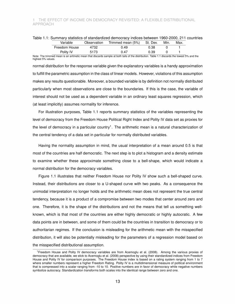
Table 1.1: Summary statistics of standardized democracy indices between 1960-2000, 211 countriesVariable Observation Trimmed mean (5%) St. Dev. Min. Max.
Freedom House 4732 0.49 0.38 0 1Polity IV 5173 0.47 0.39 0 1
Note: The trimmed mean is an aritmetic mean that discards sample at both tails of the distribution. Table 1.1 discards the lowest 5% and thehighest 5% values.
normal distribution for the response variable given the explanatory variables is a handy approximation
to fulfill the parametric assumption in the class of linear models. However, violations of this assumption
makes any results questionable. Moreover, a bounded variable is by definition not normally distributed
particularly when most observations are close to the boundaries. If this is the case, the variable of
interest should not be used as a dependent variable in an ordinary least squares regression, which
(at least implicitly) assumes normality for inference.
For illustration purposes, Table 1.1 reports summary statistics of the variables representing the
level of democracy from the Freedom House Political Right Index and Polity IV data set as proxies for
the level of democracy in a particular country1. The arithmetic mean is a natural characterization of
the central tendency of a data set in particular for normally distributed variables.
Having the normality assumption in mind, the usual interpretation of a mean around 0.5 is that
most of the countries are half democratic. The next step is to plot a histogram and a density estimate
to examine whether these approximate something close to a bell-shape, which would indicate a
normal distribution for the democracy variables.
Figure 1.1 illustrates that neither Freedom House nor Polity IV show such a bell-shaped curve.
Instead, their distributions are closer to a U-shaped curve with two peaks. As a consequence the
unimodal interpretation no longer holds and the arithmetic mean does not represent the true central
tendency, because it is a product of a compromise between two modes that center around zero and
one. Therefore, it is the shape of the distributions and not the means that tell us something well-
known, which is that most of the countries are either highly democratic or highly autocratic. A few
data points are in between, and some of them could be the countries in transition to democracy or to
authoritarian regimes. If the conclusion is misleading for the arithmetic mean with the misspecified
distribution, it will also be potentially misleading for the parameters of a regression model based on
the misspecified distributional assumption.1Freedom House and Polity IV democracy variables are from Acemoglu et al. (2008). Among the various proxies of
democracy that are available, we stick to Acemoglu et al. (2008) perspective by using their standardized indices from FreedomHouse and Polity IV for comparison purposes. The Freedom House index is based on a rating system ranging from 1 to 7where smaller numbers represent a higher Freedom Rating. Polity IV is a multidimensional measure of political environmentthat is compressed into a scalar ranging from -10 to 10. Positive numbers are in favor of democracy while negative numberssymbolize autocracy. Standardization transforms both scales into the identical range between zero and one.
13
1 THE EFFECT OF INCOME ON DEMOCRACY REVISITED: A FLEXIBLE DISTRIBUTIONALAPPROACH
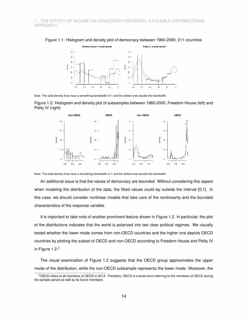
Figure 1.1: Histogram and density plot of democracy between 1960-2000, 211 countries
Note: The solid density lines have a smoothing bandwitdth of 1 and the dotted ones double the bandwidth.
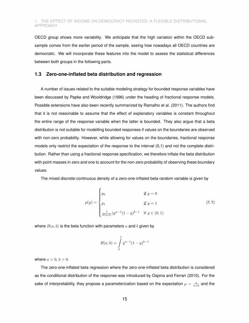
Figure 1.2: Histogram and density plot of subsamples between 1960-2000, Freedom House (left) andPolity IV (right)
Note: The solid density lines have a smoothing bandwitdth of 1 and the dotted ones double the bandwidth.
An additional issue is that the values of democracy are bounded. Without considering this aspect
when modeling the distribution of the data, the fitted values could lay outside the interval [0,1]. In
this case, we should consider nonlinear models that take care of the nonlinearity and the bounded
characteristics of the response variable.
It is important to take note of another prominent feature shown in Figure 1.2. In particular, the plot
of the distributions indicates that the world is polarized into two clear political regimes. We visually
tested whether the lower mode comes from non-OECD countries and the higher one depicts OECD
countries by plotting the subset of OECD and non-OECD according to Freedom House and Polity IV
in Figure 1.2.2
The visual examination of Figure 1.2 suggests that the OECD group approximates the upper
mode of the distribution, while the non-OECD subsample represents the lower mode. Moreover, the2OECD refers to all members of OECD in 2014. Therefore, OECD is a loose term referring to the members of OECD during
the sample period as well as its future members.
14
1 THE EFFECT OF INCOME ON DEMOCRACY REVISITED: A FLEXIBLE DISTRIBUTIONALAPPROACH
OECD group shows more variability. We anticipate that the high variation within the OECD sub-
sample comes from the earlier period of the sample, seeing how nowadays all OECD countries are
democratic. We will incorporate these features into the model to assess the statistical differences
between both groups in the following parts.
1.3 Zero-one-inflated beta distribution and regression
A number of issues related to the suitable modeling strategy for bounded response variables have
been discussed by Papke and Wooldridge (1996) under the heading of fractional response models.
Possible extensions have also been recently summarized by Ramalho et al. (2011). The authors find
that it is not reasonable to assume that the effect of explanatory variables is constant throughout
the entire range of the response variable when the latter is bounded. They also argue that a beta
distribution is not suitable for modelling bounded responses if values on the boundaries are observed
with non-zero probability. However, while allowing for values on the boundaries, fractional response
models only restrict the expectation of the response to the interval (0,1) and not the complete distri-
bution. Rather than using a fractional response specification, we therefore inflate the beta distribution
with point masses in zero and one to account for the non-zero probability of observing these boundary
values.
The mixed discrete-continuous density of a zero-one-inflated beta random variable is given by
p(y) =
p0 if y = 0
p1 if y = 1
1B(a,b) )y
a−1(1− y)b−1 if y ∈ (0, 1)
(1.1)
where B(a, b) is the beta function with parameters a and b given by
B(a, b) =
1ˆ
0
ya−1(1− y)b−1
where a > 0, b > 0.
The zero-one-inflated beta regression where the zero-one-inflated beta distribution is considered
as the conditional distribution of the response was introduced by Ospina and Ferrari (2010). For the
sake of interpretability, they propose a parameterization based on the expectation µ = aa+b and the
15

1 THE EFFECT OF INCOME ON DEMOCRACY REVISITED: A FLEXIBLE DISTRIBUTIONALAPPROACH
scale parameter vector σ = 1a+b+1 with µ ∈ (0, 1) and σ ∈ (0, 1). We also replace the probabilities
for zero and one by the parameters ν = p0/p2 and τ = p1/p2 where p2 = 1 − p0 − p1 is the
probability observing a response from the continuous part of the zero-one-inflated beta distribution.
This parameterisation ensures that the probabilities for zero, one and the continuous part add up to
one.
Furthermore, we let yit be independent random variables where each yit follows the density in
(1.1) with mean µit, unknown scale parameter σit and zero/one inflation parameters νit and τit, while
t = 1, . . . , T and i = 1, . . . , N index the time dimension and the individuals, respectively. To relate the
parameters of the zero one inflated beta distribution to regression predictors, we apply suitable link
functions, i.e.
µit =exp(ηµit)
1 + exp(ηµit)σit =
exp(ησit)
1 + exp(ησit)νit = exp(ηνit) τit = exp(ητit) (1.2)
where ηµit, ησit, η
νit and ητit are regression predictors constructed from a set of covariates. The logit
transformation applied to the mean and scale parameter enables a log odds ratio interpretation for
two observations that only differ by one unit in the variable of interest. In contrast, the natural log
transformation for the zero/one inflation parameters is directly interpretable since it is approximately
proportional to differences.
Note that the model allows us to account for heteroscedasticity due to the regression effects on
σit and µit since the variance of yit
Var(yit) =µit(1− µit)1 + ait + bit
(1.3)
is also a function of the mean µit and proportional to the scale parameter σit = 1/(1 + ait + bit).
Even though the approach by Papke and Wooldridge (1996) also does not exclude the boundary
values, it is more suitable when the truly fractional component of the response is dominant. Con-
versely, the inflated beta regression better matches our data sets because we observe a large fraction
of zeros and ones. Furthermore, the fully parametric approach used by assuming a beta distribution
for the fractional response variable leads to more efficient ML estimators (Ospina and Ferrari, 2010).
1.4 Model specification
Our study estimates a similar model to Acemoglu et al. (2008)3. We use Maddison historical3Linear model with country fixed-effects
16

1 THE EFFECT OF INCOME ON DEMOCRACY REVISITED: A FLEXIBLE DISTRIBUTIONALAPPROACH
GDP per capita4 for a robustness check of measurement error and missing values. Hence, we have
the combination of two democracy variables and two income per capita variables. We add a dummy
variable for OECD membership, which acts as an additional regressor in each model. We implement a
linear model structure with fixed-effects under the assumption that the response follows the zero-one
inflated beta distribution where the basic predictor structure is given by
ηit = β1yit−s + β2x1it−s + β3x2it + ϑi + δt (1.4)
where x1it−s is log income per capita of country i at time t − s, x2it is the OECD dummy of country
i at time t, ϑi is a country-specific fixed effect, δt is a time-specific fixed effect, and the predictor is
linked to the parameters of the response distribution via the link functions discussed above. For the
lagged part in the predictor, we used s = 1 for yearly data5, s = 5 for five year, s = 10 for ten year and
s = 20 for twenty year data, respectively. We use five year averages of data t = x5 and their first lag
in equation 1.2 to mitigate endogeneity. We also employ the lagged values of explanatory variables
for the same purpose as well as to design the causality relationship. To fit zero-one-inflated beta
regression models, we used the R-package gamlss ((Rigby and Stasinopoulos, 2005; Stasinopoulos
et al., 2008).
Because the zero-one-inflated beta regression allows us to estimate not only the mean as a func-
tion of the explanatory variables but also the scale parameter, which is proportional to the variance,
and the two probabilities for zero and one inflation, we can infer the causes of potential non-constant
variance, as well as other distributional features of democracy at time t. Despite having a relatively
suitable distributional assumption and some treatment for other statistical challenges, we do not
claim that our estimation has a rigorous causal interpretation. Instead, our intention is to provide
a benchmark for future related research.
1.5 Results
The main results of our model for different time intervals are presented in Table 1.2. The first
column shows the model estimated with yearly data (model M1), the second to fourth column with
five (M2), ten (M3), and twenty year (M4) intervals data and the last column is for five-year average
data (M5). In each model, estimated coefficients are presented for the equation for µ which represents4 Maddison GDP per capita is from Bolt and van Zanden (2013) with authors’ adjustment.5For s = 1, we jointly estimate the coefficients of mean and scale parameters with the previous four lags.
17

1 THE EFFECT OF INCOME ON DEMOCRACY REVISITED: A FLEXIBLE DISTRIBUTIONALAPPROACH
the mean of the beta distribution, the equation for σ which relates to the scale parameter of the beta
distribution and the equations for ν and τ which relate to the probabilities for zero and one inflation,
respectively.
The estimated coefficients for income per capita in the equation for µ are only significant in model
(M3), in which a ten year interval and a ten year lag structure is used. In the equation for σ income
is significant in model (M1), model (M2) and model (M5), suggesting that for annual, five year and
twenty year data income influences the variance of democracy. The negative and significant income
coefficient found for the ten year lag in the equation for ν indicates that a higher income per capita
level leads to a lower probability of a country having a value of zero (autocracy) than a value between
zero and one in the next ten years. The stronger evidence comes from the equation for τ . The positive
and significant coefficient of income (for five, ten and twenty year lags) suggests that a higher income
induces a higher probability of a country having a value of one (democracy outcome) than a value
between zero and one.
The OECD dummy is also significant in the equations for µ and σ in some cases. The positive sign
in the equation for µ reflects the higher level of democracy on average for OECD members relative to
non-OECDs. Meanwhile, the positive sign in the equation for σ indicates that the OECD group has a
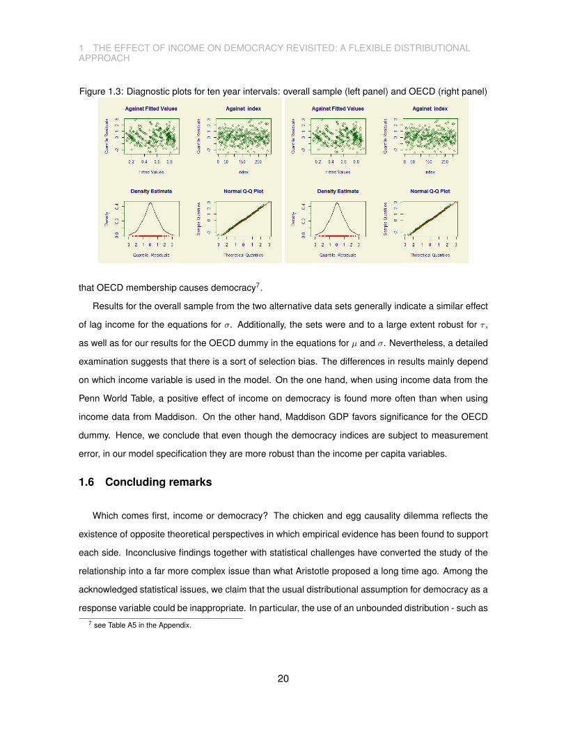
higher variance. This confirms the findings in Figure 1.2. The diagnostic plots for ten year intervals are
provided in Figure 1.3. Our estimation for the OECD versus non-OECD subsamples (see Table 1.4)
shows that the effect of income on democracy is only statistically significant in the OECD countries.
As a comparison, we provide results for the Polity IV data using income from Maddison in Table
1.36.
Table 1.3 suggests that our findings are not robust for the equations for µ , ν and τ , yet it is
more robust for the equations for σ. Past income explains the non-constant variance of democracy
through the equation for σ. The difference between the OECD and non-OECD groups is more
apparent here. The dummy for OECD countries is significant and positive in the equation for µ in
three cases, suggesting that OECD countries have higher democracy indices. The OECD dummy
is also positive and statistically significant in the equation for τ in two cases, signaling that OECD
membership increases the probability of being completely democratic. However, there is no evidence
6 see Table A1-A4 in the Appendix for the results obtained using other data set combinations.
18

1 THE EFFECT OF INCOME ON DEMOCRACY REVISITED: A FLEXIBLE DISTRIBUTIONALAPPROACH
Table 1.2: Freedom House and Penn World Table GDP per capitaDependent variable: 5 year 10 year 20 year 5 year average
democracy (M1) (M2) (M3) (M4)Mean equation (µ)
Lag democracy 1.152*** -0.855*** -2.303*** 1.978***(0.174) (0.268) (0.346) (0.183)
Lag log income per capita -0.040 0.576** -0.412 -0.071(0.154) (0.285) (0.505) (0.149)
OECD(D) 2.204** 2.354*** 0.194 2.746**(0.981) (0.675) (0.728) (1.251)
Country fe Yes Yes Yes YesYear fe Yes Yes Yes Yes
Scale equation (σ)Lag Democracy -*** + No +
Lag log income per capita +** + No -OECD(D) + - No +Country fe No No No No
Year fe Yes No No YesZero inflation equation (ν)
Lag democracy -1.829** 2.176 154.885 -3.989***(0.853) (2.277) (1.482e+5) (1.518)
Lag log income per capita 0.318 0.672 -131.339 1.539(0.807) (1.734) (7.539e+4) (1.044)
OECD(D) -44.397 -1.315 -14.103 -22.723(7.260e+6) (4.827e+6) (1.015e+7) (2.592e+4)
Country fe Yes Yes Yes YesYear fe Yes Yes Yes Yes
One inflation equation (τ )Lag democracy 9.343*** 5.534** -8.737 20.714***
(2.553) (2.475) (5.984) (6.695)Lag log income per capita 4.689** 11.383*** 15.641*** 3.183
(1.982) (3.183) (4.802) (3.460)OECD(D) 1.482 -0.173 7.887 -3.788
(8.206e+5) (4.538) (0.114) (9.766e+3)Country fe Yes Yes Yes Yes
Year fe Yes Yes Yes YesObservation 729 317 112 753
Country 118 106 69 119Global deviance -191.098 -158.131 -168.271 -505.7995
AIC 602.902 527.869 277.729 282.201SBC 2425.797 1817.172 883.954 2094.55
The coefficients are in logit form for the equations for µ and σ, in log form for the equations for ν and τ . The equation for σ only shows thedirection of relationship and its significance level. Significance levels are 0.1 (*), 0.05 (**) and 0.01 (***). Standard errors are in parentheseswith “qr” type, which assumes there is no correlation among the parameters. Models M1-M3 are estimated using 5, 10 and 20 year intervals,respectively. Country fixed-effects and year fixed-effects are used only when the algorithms converge.
19
1 THE EFFECT OF INCOME ON DEMOCRACY REVISITED: A FLEXIBLE DISTRIBUTIONALAPPROACH
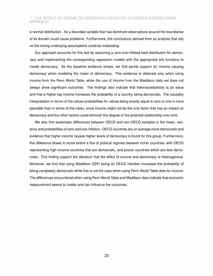
Figure 1.3: Diagnostic plots for ten year intervals: overall sample (left panel) and OECD (right panel)
that OECD membership causes democracy7.
Results for the overall sample from the two alternative data sets generally indicate a similar effect
of lag income for the equations for σ. Additionally, the sets were and to a large extent robust for τ ,
as well as for our results for the OECD dummy in the equations for µ and σ. Nevertheless, a detailed
examination suggests that there is a sort of selection bias. The differences in results mainly depend
on which income variable is used in the model. On the one hand, when using income data from the
Penn World Table, a positive effect of income on democracy is found more often than when using
income data from Maddison. On the other hand, Maddison GDP favors significance for the OECD
dummy. Hence, we conclude that even though the democracy indices are subject to measurement
error, in our model specification they are more robust than the income per capita variables.
1.6 Concluding remarks
Which comes first, income or democracy? The chicken and egg causality dilemma reflects the
existence of opposite theoretical perspectives in which empirical evidence has been found to support
each side. Inconclusive findings together with statistical challenges have converted the study of the
relationship into a far more complex issue than what Aristotle proposed a long time ago. Among the
acknowledged statistical issues, we claim that the usual distributional assumption for democracy as a
response variable could be inappropriate. In particular, the use of an unbounded distribution - such as7 see Table A5 in the Appendix.
20

1 THE EFFECT OF INCOME ON DEMOCRACY REVISITED: A FLEXIBLE DISTRIBUTIONALAPPROACH
Table 1.3: Polity IV and Penn World Table GDP per capitaDependent variable: 5 year 10 year 20 year 5 year average
democracy (M1) (M2) (M3) (M4)Mean equation (µ)
Lag democracy 1.350*** -0.648** -2.735*** 2.432***(0.186) (0.321) (0.512) (0.183)
Lag log income per capita 0.097 0.086 -0.828 0.014(0.162) (0.315) (0.701) (0.151)
OECD (D) 2.084** 1.147 -0.380 1.779***(0.707) (0.728) (0.905) (0.636)
Country fe Yes Yes Yes YesYear fe Yes Yes Yes Yes
Scale equation (σ)Lag democracy + + No -
Lag log income per capita + - No +OECD (D) - +** No +Country fe No No No No
Year fe Yes No Yes YesZero inflation equation (ν)
Lag democracy -12.541 -8.362 3.749e-11 -29.870(6.252e+04) (9.572e+4) (1.046e+4) (7.741e+4)
Lag log income per capita -23.227 -53.219 1.283e-8 -54.215(0.851) (5,277e+4) (1.370e+4) (4.967e+3)
OECD (D) 39.884 38.252 2.074e-6 142.981(1.358e+7) (8.394e+5) (2.891e+5) (8.426e+6)
Country fe Yes Yes Yes YesYear fe No Yes Yes Yes
One inflation equation (τ )Lag democracy 30.596*** 4.794 0.512 29.946***
(2.101) (8.040) (1.573e+1) (2.404)Lag log income per capita 1.546 -9.055 1.705 9.840**
(2.955) (6.443) (2.329e+1) (4.128)OECD (D) 8.858 58.468 46.918 0.303
(9.187e+4) (2.865e+6) (6.823e+6) (4.745e+9)Country fe Yes Yes Yes Yes
Year fe Yes Yes Yes YesObservation 729 317 112 735
Country 118 106 69 119Global deviance -630.498 -262.450 -186.572 -861.350
AIC 165.503 423.550 259.429 -73.350SBC 1992.989 1712.853 865.654 1739.000
The coefficients are in logit form for the equations for µ and σ, in log form for the equations for ν and τ . The equation for σ only shows thedirection of relationship and its significance level. Significance levels are 0.1 (*), 0.05 (**) and 0.01 (***). Standard errors are in parentheseswith “qr” type, which assumes there is no correlation among the parameters. Models M1-M3 are estimated using 5, 10 and 20 year intervals,respectively. Country fixed-effects and year fixed-effects are used only when the algorithms converge.
21

1 THE EFFECT OF INCOME ON DEMOCRACY REVISITED: A FLEXIBLE DISTRIBUTIONALAPPROACH
Table 1.4: Freedom House and Penn World Table GDP per capita for sub samplesDependent 5 year 10 year 5 year average
variable: OECD non-OECD OECD non-OECD OECD non-OECDdemocracy (M1) (M2) (M3) (M4) (M5) (M6)
Mean equation (µ)Lag democracy 1.187*
(0.713)1.014***(0.171)
-7.406***(0.495)
-0.711**(0.279)
2.598***(0.599)
2.054***(0.176)
Lag log income per capita 1.002*(0.587)
-0.190(0.164)
2.859***(0.444)
0.242(0.295)
-0.119***(0.586)
-0.123(0.151)
Country fe Yes Yes Yes Yes Yes YesYear fe Yes Yes Yes Yes Yes Yes
Scale equation (σ)Lag democracy -*** -** -*** + -*** +
Lag log income per capita -*** +* - -* -*** -Country fe No No No No No No
Year fe No Yes No No No NoZero inflation equation (ν)
Lag democracy 42.913(1.207e+7)
-2.239**(0.924)
4.917e-7(8.748e+6)
1.899(2.208)
5.377e-7(1.709e+5)
-3.837**(1.493)
Lag log income per capita -10.302(2.269e+7)
0.333(0.674)
-3.062e-7(8.518e+6)
1.525(1.662)
-3.432e-7(1.700e+5)
0.350(0.881)
Country fe Yes Yes Yes Yes Yes YesYear fe Yes Yes Yes Yes Yes Yes
One inflation equation (τ )Lag democracy 44.020*** 7.777*** 14.450 9.421** 21.314* 34.933***
(15.870) (2.586) (9.651) (3.976) (11.300) (11.301)Lag log income per capita -2.225
(4.302)7.293***(2.708)
9.523**(3.901)
31.863***11.800
-11.976***(2.652)
18.967*(11.096)
Country fe Yes Yes Yes Yes Yes YesYear fe Yes Yes No Yes Yes Yes
Observation 229 579 114 234 215 533Country 29 101 28 86 28 87
Global deviance -89.181 -187.327 -74.626 -158.414 -108.734 -497.553AIC 154.819 498.673 133.374 399.586 123.266 104.447SBC 573.733 1994.6 417.939 1363.621 514.260 1392.282
The coefficients are in logit form for the equations for µ and σ, in log form for the equations for ν and τ . The equation for σ only shows thedirection of relationship and its significance level. Significance levels are 0.1 (*), 0.05 (**) and 0.01 (***). Standard errors are in parentheseswith “qr” type, which assumes there is no correlation among the parameters. Models M1-M3 are estimated using 5, 10 and 20 year intervals,respectively. Country fixed-effects and year fixed-effects are used only when the algorithms converge.
22
1 THE EFFECT OF INCOME ON DEMOCRACY REVISITED: A FLEXIBLE DISTRIBUTIONALAPPROACH
a normal distribution - for a bounded variable that has dominant observations around the boundaries
of its domain could cause problems. Furthermore, the conclusions derived from an analysis that rely
on the wrong underlying assumptions could be misleading.
Our approach accounts for this fact by assuming a zero-one-inflated beta distribution for democ-
racy and implementing the corresponding regression models with the appropriate link functions to
model democracy. As the baseline evidence shows, we find partial support for income causing
democracy when modeling the mean of democracy. This evidence is obtained only when using
income from the Penn World Table, while the use of income from the Maddison data set does not
always show significant outcomes. The findings also indicate that heteroscedasticity is an issue
and that a higher lag income increases the probability of a country being democratic. The causality
interpretation in terms of the values probabilities for values being exactly equal to zero or one is more
plausible than in terms of the mean, since income might not be the only factor that has an impact on
democracy and the other factors could diminish the degree of the potential relationship over time.
We also find systematic differences between OECD and non-OECD samples in the mean, vari-
ance and probabilities of zero and one inflation. OECD countries are on average more democratic and
evidence that higher income causes higher levels of democracy is found for this group. Furthermore,
this difference draws to some extent a line of political regimes between richer countries, with OECD
representing high income countries that are democratic, and poorer countries which are less demo-
cratic. This finding support the literature that the effect of income and democracy is heterogenous.
Moreover, we find that using Maddison GDP, being an OECD member increases the probability of
being completely democratic while this is not the case when using Penn World Table data for income.
The differences encountered when using Penn World Table and Maddison data indicate that economic
measurement seems to matter and can influence the outcomes.
23

2 OPPORTUNITIES IN EDUCATION: ARE FACTORS OUTSIDE INDIVIDUAL RESPONSIBILITYREALLY PERSISTENT? EVIDENCE FROM INDONESIA 1997-2007
2 Opportunities in Education: Are Factors Outside IndividualResponsibility Really Persistent? Evidence from Indonesia1997-2007
Abstract
Education is a strong predictor of economic performance. Educational inequality in opportunity
could thus make a significant contribution to earning disparities. Following Ferrerira and Gignoux
(2014) parametric method, we construct aggregate indices of inequality in educational opportunities
for thirteen Indonesian provinces in the years 1997, 2000 and 2007. The contribution of this paper
is to define individual indices of the power of circumstances, which measure the effect that the
accumulation of factors, outside individual control, has on individual educational achievements and
earnings in the short and long run. We find that-for the period considered- there has been a declining
trend in inequality of educational opportunities, albeit not in all provinces. Our findings also suggest
that parental educational background is the most significant factor for school survival. Additionally,
the effect that circumstances exert on future individual educational achievements and early earnings
perspectives tends to persist over time, but only to a very small extent. Our causal model, which
relates educational budget policy to equality of opportunity, shows that the educational budget has
a negative impact on the youngest cohorts, thus causing us to question the effectiveness of the
allocation of resources to primary and intermediate schools.
Based on a joint work with Maria C. Lo Bue.
24
2 OPPORTUNITIES IN EDUCATION: ARE FACTORS OUTSIDE INDIVIDUAL RESPONSIBILITYREALLY PERSISTENT? EVIDENCE FROM INDONESIA 1997-2007
2.1 Introduction
It has been well recognized that a person’s educational achievement is not only a key dimension
of her human development in its own right, but also represents a fundamental input for the realization
of other human development goals, such as wealth, health, employment and political participation.
More recently, a number of studies has also shown that both within and across countries, inequalities
in education are likely to be reflected in disparities in other dimensions. The existence of such
correlations has raised political and academic interest in the inequality of education and, in particular,
two questions have emerged: which factors are driving these inequalities? Are they all “unfair”?
The theory of inequality of opportunity can provide an answer to these questions as it finds its
main rationale in the idea that inequality itself can have different sources, but not all of these can
be equally objectionable. As theoretically conceptualized by Roemer (1998), differences on certain
socio-economic outcomes may be partly attributed to individual choices, innate ability, talents and
efforts and partly to factors or circumstances which are economically exogenous to the person, such
as gender and socio-economic background.
While inequalities in education that are due to personal responsibility are fair and do not necessar-
ily need to be suppressed, disparities in educational achievements, which result from factors beyond
an individual’s control are, without doubt, inequitable, and should be amenable to equal-opportunity
policy interventions that, as suggested by Roemer, will equalize advantages for each centiles of the
efforts distribution, across groups of people, which share the set of circumstances.
Empirical evidence regarding this issue is still less explored. However, OECD (2012) suggests
the positive relationship between educational opportunities and labour income. Therefore, educa-
tional policies with strong attention on equity could be used as a strategic tool to improve economic
performance in a long term.
Equality of opportunity could only be achieved when pre-determined circumstances have no cor-
relation with success in life (de Barros et al., 2008). In the case of education, pre-determined circum-
stances should not affect the chance of children going to school or achieving identical educational
performance.
Among developing countries, evidence using PISA scores 2006 placed Indonesia in the lower half
of cross-country distribution of inequality in educational opportunity (Ferrerira and Gignoux, 2014).
Contrarily, the Indonesian GINI index shows an increasing trend from 31.3 in 1996 to 33 in 2004 and
25

2 OPPORTUNITIES IN EDUCATION: ARE FACTORS OUTSIDE INDIVIDUAL RESPONSIBILITYREALLY PERSISTENT? EVIDENCE FROM INDONESIA 1997-2007
38.1 in 2011 (World Bank, 2014), which indicates that educational policies might not have accurately
targeted equity.
In this paper, we therefore focus on country level evidence using household data from the Indone-
sian Family Life Survey (IFLS), in order to quantify the role that the accumulation of pre-determined
circumstances play in influencing future socio-economic outcomes and generating inequality in edu-
cational opportunities among the Indonesian population over the period 1997-2007.
We contribute to previous literature by devising an individual index of the power of circumstances,
which explains the influence that the accumulation of pre-determined circumstances has on individual
educational achievements. This allows us to see how persistent these circumstances can be over the
individual life’s course and, thus, how sticky current levels of inequality of opportunities can be.
Next, by evaluating the association between our power of circumstances index and educational
budgeting at the provincial level, we seek to understand if the educational budgeting policy had any
influence (and in which direction) on inequality of opportunity in education.
The remainder of this paper is organized as follows. Section 2.2 is devoted to providing a review
of the literature in this field and Section 2.3 discusses methodological issues involved in measuring
inequality of educational opportunity and the specific choices we have made. In Section 2.4 we report
descriptive statistics and discuss our empirical findings in Section 2.5. Section 2.6 concludes.
2.2 Inequality of opportunity: conceptual underpinnings and empirical appli-
cations
The concept of inequality in educational opportunity finds its roots in the mid-60s when the Cole-
man Report (Coleman et al., 1966) started the debate on what is meant by equality of opportunity
and how to achieve it. This report questioned the effectiveness (in terms of a fairer distribution of
outputs or educational achievements) of policies aimed at equalizing benefits between students or
granting full access to education and argued that socio-economic conditions and family background
are important factors that drive most of the variation in students’ achievements.
The debate on the meaning of equality of opportunity in various income and wealth related out-
comes was enriched by the contributions of important philosophers and economists (such as Rawls
1971; Nozick 1974; Sen 1980, 1985; Dworkin 1981a,b) posited the importance of compensating
individuals” different situations, especially in cases outside of an individual’s personal responsibility. It
was only at the end of the nineties that this concept was explicitly addressed, described and translated
26
2 OPPORTUNITIES IN EDUCATION: ARE FACTORS OUTSIDE INDIVIDUAL RESPONSIBILITYREALLY PERSISTENT? EVIDENCE FROM INDONESIA 1997-2007
into a mathematical formulation in John Roemer’s seminal book on equality of opportunity (1998).
The main argument of Roemer was based on the distinction between unchosen and pre-determined
circumstances and individual efforts. While the latter are attributed to the personal responsibility of the
individual, the former are inherited by the individual and are beyond his or her control. Differences in
individual outcomes which are attributable to circumstances are hence not only morally objectionable
but can also lead to an inefficient allocation of resources (Ferrerira and Gignoux, 2014; Fernández
and Galí, 1999) and should thus be compensated by public policies. On the other hand, outcome
differences that are due to individual choices and personal responsibility can be ethically accepted
because they represent the natural reward of individual effort (see Fleurbaey 2008).
Measuring inequality of opportunity requires two fundamental preliminary steps: first, the search
of a set of factors which can accurately represent those circumstances and second, the partition of
a society into groups (or types) of individuals sharing the same set of circumstances and into groups
(or tranches) of individuals characterized by the same degree of effort (Checchi and Peragine, 2010).
Two methodological approaches have been suggested in order to quantify the extent to which a
given society is unequal. Either one can adopt an utilitarian “ex-ante” perspective (van der Gaer,
1993) by considering outcome differences between types- prior to the realization of their effort level,
or one can follow an “ex-post” approach by looking at the opportunity set granted to individuals
who exert the same degree of effort (Roemer, 1998; Checchi and Peragine, 2010). While in the
first approach equality of opportunity is achieved when opportunities are equalized between types
(Ferrerira and Gignoux, 2011, 2014), in the ex-post approach outcomes should be equalized within
tranches or groups of people who, independently of their inherited circumstances, are featured by the
same degree of effort (Checchi and Peragine, 2010). As noted in Fleurbaey (2008) and Checchi and
Peragine (2010) these two approaches do not necessarily generate same rankings of distributions, as
compensation mechanisms within types will only affect opportunity inequality when adopting the ex-
post approach (Checchi and Peragine, 2010). On the other hand, the ex-ante approach can generate
a distribution that fully satisfies the utilitarian or reward principle according to which inequality of a
given outcome within groups of individuals sharing the same circumstances can be fair, as long as
these individuals are rewarded according to the amount of effort exerted in order to achieve a certain
outcome (Donni and Pignataro, 2014).
The vast majority of the applied studies on the measurement of inequality of opportunity has fo-
cused on the opportunities for the acquisition of income (see, among others, Peragine 2002, 2004a,b;
27
2 OPPORTUNITIES IN EDUCATION: ARE FACTORS OUTSIDE INDIVIDUAL RESPONSIBILITYREALLY PERSISTENT? EVIDENCE FROM INDONESIA 1997-2007
Bourguignon et al. 2007; Peragine and Serlenga 2008; Lefranc et al. 2008, 2009; Aaberge et al.
2011; Björklund et al. 2012; Andreoli et al. 2014) whereas relatively fewer empirical studies appear
in the domain of education. In this field, three main strands of research have emerged so far: the
first strand of the empirical literature has applied the “education production function” framework to
directly estimate the effect of specific socio-economic variables on educational outcomes (Fertig 2000;
Hanushek 1979; Wößmann 2003; Filmer and Pritchett 1998) and to directly as well as indirectly
consider intergenerational mobility in educational achievements outcomes (Behrman et al., 2001;
Dahan and Gaviria, 2001; Lam and Schoeni, 1993).
The second, more recent strand of the literature has addressed the Roemer’s theory more ex-
plicitly and attempted to operationalize the concept of inequality of opportunity theory in the domain
of education. Some notable contributions include the study by Ferrerira and Gignoux (2014) who
propose and compute an ex-ante, parametric measure of inequality of educational opportunity for
PISA scores in 57 countries; the article by Asadullah and Yalonetzky (2012) who construct several
indices of inequality in educational opportunity across Indian states and the analysis conducted
by Gamboa and Waltenberg (2012) who, following an ex-ante non-parametric approach, considers
inequality of educational opportunity in PISA scores for Latin American students.
Lastly, the third strand of the literature (Mongan et al., 2011; Waltenberg and Vandenberghe, 2007;
Iatarola and Stiefel, 2003) has instead focused more on policy-oriented research objectives and has
evaluated the opportunity-equalizing effects of education policies.
This paper connects these three strands by considering the distribution of educational oppor-
tunities across provinces and over time, assessing the role that both circumstances and individual
responsibility plays in education levels and earning outcomes in the short and long run, and evaluating
the effect of educational budgeting policies on inequality of opportunity.
2.3 Methods
2.3.1 Measuring inequality of opportunity in education
To measure the educational inequality of opportunity, we seek to build upon Roemer’s utilitarian
principle, according to which inequality between individuals determined by different degrees of effort
is fair (Donni and Pignataro, 2014). We thus pursue the ex-ante approach that considers inequality of
28

2 OPPORTUNITIES IN EDUCATION: ARE FACTORS OUTSIDE INDIVIDUAL RESPONSIBILITYREALLY PERSISTENT? EVIDENCE FROM INDONESIA 1997-2007
opportunity as a between-type inequality1. For the main educational outcome variable we focus on
educational attainment, which is completed years of schooling defined by the last grade the individual
achieved in order to avoid measurement error (i.e. the same real year of schooling could reflect
different educational levels).
Following Bourguignon et al. (2007) and Ferrerira and Gignoux (2014), we apply a parametric
methodology to construct our aggregate indices of the inequality of opportunity in education (mea-
sured by the educational attainment):
θIoP =V ar
(Ci, β
)V ar (Yi)
, (2.1)
which is simply the R-squared of an Ordinary Least Squares (OLS) regression of the individual’s
educational achievement (y) on a vector C of individual circumstances.
As argued in Dardanoni et al. (2005), the exact content of these circumstances is a contentious
issue which is largely related to the outcome the research is focused on. For example, one can
reasonably assume to have one set of circumstances defining types when examining inequality of
opportunity for educational attainments (where parental wealth and education may play a central
role) and another set when the outcome variable is represented by earnings or other labor market
achievements (where gender becomes a key variable).
Among the pre-determined circumstances available, we therefore stick to variables that were
also proposed in the precedent literature, ones that are truly “pre-determined” and exogenous and
have a small rate of missing values to keep the attrition rate low. Those are parental education,
represented by mother and father educational attainments, sex, rural or urban residence and dummies
of household wealth such as ownership of the house, other buildings, farm land, livestock, vehicles,
household appliances, savings, receivables, jewelry, furniture, electricity, television and other assets.
Contrary to Ferrerira and Gignoux (2014), we do not include access to books as this variable might
actually be endogenous, i.e. parents observing efforts and school achievements of their kids might
motivate them to buy more books and learning tools to satisfy the increasing needs of their keenest
children.1The ex-ante approach is well represented in the related empirical literature and has been adopted by Bourguignon et al.
(2007); Checchi and Peragine (2010); Ferreira and Gignoux (2011, 2014), Li Donni et al. (2014).
29

2 OPPORTUNITIES IN EDUCATION: ARE FACTORS OUTSIDE INDIVIDUAL RESPONSIBILITYREALLY PERSISTENT? EVIDENCE FROM INDONESIA 1997-2007
It is important to note that since all the variables included in this analysis are not all of the
possible pre-determined circumstances, the R-squared should be interpreted as the lower bound
of educational inequality of opportunity2.
Further, we do not include age as one of the explanatory variables of educational attainments.
We argue that regardless of whether age is truly exogenous and pre-determined, it makes very little
sense to consider it as a circumstance that may drive inequality of opportunity3. In our approach we
thus consider the adjusted educational attainment as the main dependent variable which results from
the residual obtained from two sets of zero-truncated Poisson regressions of educational attainment
against age, runned separately for two cohorts of individuals. By doing this, we make sure that the
effect of age is somewhat controlled for and avoid the risk of obtaining a blurred measure of inequality
of opportunity.
Excluding the constant, equation 2.2 proceeds the extraction of educational attainment from age
that yields the residual part Y as the age-adjusted educational attainment for each cohort, where
subscriptions index i and t represent individual and time consecutively4.
Educational attainmentit = Ageit + Yit (2.2)
Primary education in Indonesia normally starts at the age of 6 and the adequate supply of primary
schools implies that 6-10 years old have a similar level of opportunity in education. Consequently, we
define our youngest cohort as 11-14 years old and the next cohort as 15-18 years old5.
After having obtained our aggregate indices of inequality of opportunity for all the Indonesian
provinces sampled in IFLS for the three different time periods (i.e. 1997, 2000 and 2007), we are able
to analyze time trends and differences among provinces in inequality of opportunity of education.
2A formal proof is provided in Ferreira and Gignoux (2011). In practise, it is also crucial to check the adjusted R-squaredwhen selecting the circumstances. The arbitrarily large disparity between R-squared and adjusted R-squared indicates thatsome of the explanatory variables do not significantly explain the outcomes.
3and when the outcome is educational attainment, the inclusion of age as one of the regressors in OLS will considerablyinflate the R-squared.
4We argue that while the residuals are indeed generated from a Poisson model, it is sensible to flexibly make a furtherassumption in the second stage regression that age-adjusted educational attainment is normally distributed as the residualsfrom the first stage regression have no longer count nature as well as they could possess negative values.
5Basic descriptive statistics are reported in Table B1 in the Appendix.
30
2 OPPORTUNITIES IN EDUCATION: ARE FACTORS OUTSIDE INDIVIDUAL RESPONSIBILITYREALLY PERSISTENT? EVIDENCE FROM INDONESIA 1997-2007
Lastly, by applying the Shapley value method (Shorrock, 1999, 2013), we can decompose our
index of educational inequality of opportunity and find the contribution of each of the circumstances6.
2.3.2 Measuring the effect of individual circumstances
While the R-squared is able to measure the extent to which educational opportunities are dis-
tributed among a given groups at the aggregate level, there is one important question left. To what
extent do we, as the researchers, use this measure Ferrerira and Gignoux (2014) have shown that
the R-squared of pre-determined circumstances explaining PISA score in each country is significantly
associated with two educational policy variables. While the approach is definitely promising, it has
the drawback that this aggregate measure cannot explain the effect of inequality of opportunity on the
individual level. Instead, it might be of crucial importance to explain if and how the “burden” of unequal
opportunities in education carried by each person will affect her future life achievements, such as the
educational attainment, wage, occupation, income, productivity or non-cognitive ability to name a few.
We therefore rely on the longitudinal dimension of the dataset and find an alternative measure that is
able to capture the inequality of opportunity in that sense.
We focus our attention on the fitted values of a regression model that are comparable to the R-
squared to grasp the idea of the inequality of opportunity at the individual level. In a simple linear
regression setting where the dependent variable is the adjusted years of education observed for
individual i at time t in each cohort and a vector of circumstances X such as7:
Yit = α+ βXitc + δ2Z2 + ...+ δnZn + γt + µit (2.3)
and E (µit) = 0, the fitted values of each individual i, i = 1, ..., n at time t, t = 1, ..., T for each
cohort c excluding the common constant and time effect as well as individual effects are simply given
by:
Yit = βXit (2.4)
6In the Shapley decomposition, the contribution of each factor is determined as average marginal contribution taken over allpossible ways in which factors may be removed in sequence.
7For clarification, Yit in eq.2.3 is an estimated Yit in Eq. 2.2.
31
2 OPPORTUNITIES IN EDUCATION: ARE FACTORS OUTSIDE INDIVIDUAL RESPONSIBILITYREALLY PERSISTENT? EVIDENCE FROM INDONESIA 1997-2007
The R-squared of this model informs us of the extent to which the variation of X explains the vari-
ation in Y for all individuals i over time. The fitted value Yit explains, alternatively, the predicted value
for response variable Y of individual i at time t that is specifically influenced by the X circumstances
experienced by individual i at time t, with β governing the average magnitude of the relationship over
time and across individuals.
The interpretation of this measure is quite straightforward. Fitted values are the part of individual
educational attainment that is explained by individual pre-determined circumstances. Fitted values
also contain constant and the estimated parameter. But they are fixed terms so the distance between
two observations remains proportional and the distribution rank of the fitted values does not change.
The higher value of pre-determined circumstances in the model, hence the higher the fitted values
Y , the stronger the effect of pre-determined circumstances as the source of inequality of opportunity
at the individual level, contributes to the years of education. This one-to-one relationship is more
understandable when the fitted values are tailored to the standardized range [0,100]. Standardized
fitted values zero represent the individuals with the lowest effect of pre-determined circumstances,
while the largest values map the ones with the highest effect of pre-determined circumstances8.
Furthermore, equation 2.3 can be seen as a two-way fixed-effects regression by replacing individ-
ual dummies Z with individual time invariant effect εi for a more compact estimation procedure, such
that
Yit = α+ βXitc + γt + εi + µit (2.5)
The two-way fixed-effect estimator of equation 2.5 is defined based on
(Yit − Yi) = β(Xit − Xi) + (γt − γ) + (µit − µi) (2.6)
8Concerning the importance of explanatory variables, it is crucial to note that unlike R-squared, fitted values cannot beadjusted. Instead, it purely relies on the coefficients of pre-determined circumstances. If β is large, fitted values will be largetoo. If β is close to zero or practically insignificant, it translates into the fitted values as a very small number. This measurewill potentially suffer from imprecision if β is large but the standard error is also large that makes it statistically insignificant.Therefore, we need to keep an eye on the statistical assessment of individual coefficients such as t-test and VIF before makingdecision to move forward using fitted values, or even to refine the model until the empirical assessments are more convincing.Another issue with fitted values is related to the modelling strategy. Ordinary least square that implicitly assumes normaldistribution naturally produces unrestricted fitted values. However, in many cases educational outcomes are bounded andparticularly for educational attainment it should have the lowest value zero. Negative fitted values, when this is the case, willviolate the nature of of schooling. Therefore, generally speaking it is very important to investigate if the fitted values go beyondtheir innate boundaries and when it is there, one may have to look at various strategies to overcome this issue prior furtheranalysis.
32

2 OPPORTUNITIES IN EDUCATION: ARE FACTORS OUTSIDE INDIVIDUAL RESPONSIBILITYREALLY PERSISTENT? EVIDENCE FROM INDONESIA 1997-2007
that removes time invariant variables9. The coefficient estimates and standard errors of equation
2.3 and equation 2.5 ( as well as equation 2.6) are identical10. Nevertheless, in equation 2.5 and
2.6 the estimates have a stronger causal interpretation, such that for each individual i, the predicted
values are translated as the joint influence of pre-determined circumstances deviation at time point
t from its mean on the deviation of educational attainment at time point t from its mean11. This
interpretation employs within variation to solidify the effect of circumstances in time t relative to the
ones at every time point via an averaging procedure. This method privilege is not found for models
with cross-sectional information or longitudinal data sets with pooled approaches.
As for the term time dimension deviation from its mean (γt − γ) in equation 2.5, it exists for each
predicted value. Therefore, this does not affect the within variation attached to index of circumstances
deviation12.
Moreover, we exploit the assumption that in the individual fixed effect model, as specified in
equation 2.5, εi is the zero-mean time-invariant part of the error term. We interpret this part as
an upper-bound estimate of the fixed element of unobserved effort or innate ability . The possibility
that effort or innate ability varies over time so that it has a time-variant element is an interesting case,
yet beyond the scope of the study. We encourage the readers to peruse this topic.
2.3.3 Assessing the long-term effect of the circumstances
Once equation 2.5 is estimated to extract the individual indexes of the effect of circumstances
deviation for each time point t(4Yt
)–also referred to as the individual index of effect of circum-
stances - and of innate ability (εi), we turn to the third-stage of our analysis. This stage will focus
on the cohorts of students who stopped school by the time the last survey was taken (i.e. 2007)
and use these measures to explain long-term educational and earning outcomes. The purpose of
this stage is mainly to assess whether and to what extent the educational gains obtained during
9Some source of complete derivation is i.e. by Allison (2009).10Clustered standard errors.11The deviation implies the magnitude of pre-determined circumstances affecting the outcomes, i.e. the small deviation of
X from its mean at time t leads to a small impact on the deviation of Y from its mean at time t. In addition, deviation has twodirections, negative and positive. Pursuing pre-determined circumstances that affect the outcomes direction might utilize thisapproach.
12It is important to notice, however, that STATA routine for estimating the fixed-effect through xtreg,fe command has a bitdifferent method to produce the predicted values in order to introduce back the constant. Under the constraint that ε = 0,the fixed-effects model reformulation from Gould (2013) is modified into two-way fixed-effect version so that for each cohort(Yit − Yi − ¯Y ) = α+ β(Xit − Xi − ¯X) + γt + (µit − µi − ¯µ). The reformulation does not affect the within variation of indexof circumstances since the additional terms do not contain individual subscript i.
33

2 OPPORTUNITIES IN EDUCATION: ARE FACTORS OUTSIDE INDIVIDUAL RESPONSIBILITYREALLY PERSISTENT? EVIDENCE FROM INDONESIA 1997-2007
school-age through the beneficial effect of circumstances persist over time and contribute to long
term achievements such as educational attainment at the last survey period in 2007, enrolment in
tertiary education and wage earned as young adults.
These long term effects for each cohort are obtained from the following three sets of regressions
(we ignore the constant and error terms for simplification):
Completed years of educationi,2007 = θE( Yi,2007 − Yi) + τE εi (2.7)
which are estimated with a zero truncated Poisson model by maximum likelihood estimation;
Enrollment in universityi,2007 = θU ( Yi,2007 − Yi) + τU εi (2.8)
where the dependent variable is a dummy which equals 1 if the individual is enrolled in university
and the effects are estimated with a maximum likelihood probit model;
Log wage per dayi,2007 = θW ( Yi,2007 − Yi) + τW εi (2.9)
that is estimated with a Heckman selection model where selection is predicted by using age, years
of education, and dummies for female gender, being married, and for enrolment in university.
Equation 2.7, 2.8 and 2.9 work with two different sets of sample, observation in 1997 and obser-
vation in 2000. Hence, the average outcome over time Yi depends on when the observation entered
the survey. More specifically, for t = 1997 the outcome average Yi is estimated over the time period
1997, 2000 and 2007. While for t = 2000, Yi is from the time period 2000 and 2007.
We lastly consider the relationship between inequality of opportunity and educational budgeting
policy. In doing so, we aim to see whether allocating more resources to the education sector had any
effect on the equalization of opportunities among students and thus therefore mitigated the influence
of circumstances on individual educational achievements.
We therefore model our indexes of the effect of circumstances as a function of lagged educational
budget spending and the lagged values of the dependent variable. Our regression of interest for each
cohort takes the following form:
34

2 OPPORTUNITIES IN EDUCATION: ARE FACTORS OUTSIDE INDIVIDUAL RESPONSIBILITYREALLY PERSISTENT? EVIDENCE FROM INDONESIA 1997-2007
ˆ4Yi,p,t = ϕ+ θ ˆ4Yi,p,t−s + δbudgetp,t−x + γt + υi,p,t (2.10)
where ˆ4Yi,p,t is the individual index of the effect of circumstances measured in time t for individual
i, living in province p; ˆ4Yi,p,t−s is the lagged value of the index as measured in the previous survey
available, budgetp,t−x is the share of the budget devoted to education in province p at time t-x, where
x is two, three or five years depending on whether the dependent variable is observed in 1997, 2000
or 2007 and γt are the time fixed effects, υi,p,t is the idiosyncratic error term with zero expectation.
There is a concern that the standard errors in equation 2.7, 2.8, 2.9 and 2.10 are downward biased.
In the second stage analysis, the age adjusted attainment is an estimated variable from the first stage
analysis and the estimation excludes this kind of uncertainty. The complication of parametric inference
consequently gets bigger in the third stage analysis. We thus rely on bootstrapping to estimate the
final standard errors. In this fashion, the implicit assumption is that the sets of observations are
independently and identically distributed. We expect that this assumption holds true, as we have
included the sampling weights in the first stage analysis to correct for the probability of being selected
into the survey.
2.4 Data and Descriptive Analysis
2.4.1 Data
Our main data comes from the 1997, 2000 and 2007 waves of the Indonesia Family Life Survey
(IFLS) which is a longitudinal individual and household survey data conducted in 13 Indonesian
provinces spread out in the islands of Sumatra, Java, Kalimantan, Sulawesi, Bali and West Nusa
Tenggara.
There are interesting features in the IFLS which make this data particularly suited to our research
needs. First, the data featuresis featured by high recontact rates (Frankenberg and Thomas 2000)
that contribute significantly to data quality by lowering the bias due to non-random attrition. Second,
in addition to the information on theto basic demographic and socio-economic characteristics of all
the household’s members, the IFLS collected detailed information on various educational aspects
(e.g., current schooling grade; age at which the child first enrolled at school; number of correct
35

2 OPPORTUNITIES IN EDUCATION: ARE FACTORS OUTSIDE INDIVIDUAL RESPONSIBILITYREALLY PERSISTENT? EVIDENCE FROM INDONESIA 1997-2007
answers given in a cognitive test) as well as on earnings which are necessary to analyze inequality of
opportunity in educational outcomes and intergenerational mobility.
To scrutinize the educational budget policy, we extracted lagged annual provincial revenue data
(“Anggaran Pendapatan dan Belanja Daerah”-APBD) from The Indonesian Ministry of Finance (Min-
istry of Finance - Government of Indonesia, 1997-2007, 2007)13. The data are available for public, but
the formats are different. Data for 1994/1995 and 1996/1997 combine the budget of education, youth,
sport and faith under the same umbrella, while data in 2002 has specific section for educational
budget. Even though the correlation established for 2007 and other waves are not head-to-head
comparable, they still give some benefits regarding the general description of the relationship between
educational policies and educational inequality of opportunity.
2.4.2 Levels and trends of inequality of opportunity in education in Indonesia
Table 2.1 shows our estimates of the inequality of educational opportunity, measured as the R-
squared of a set of several regressions run separately for each province, year and cohort.
On average these figures suggests that pre-determined circumstances account for a relatively low
portion of the total variance of attainment, yet but there are remarkable differences among provinces
as well as, between cohorts and over time.
We see that –in most of the cases- the inequality of opportunity measure seems to be relatively
higher for the oldest cohorts, a finding, this one, which goes against our initial expectations. This is
due to the fact that one would reasonably assume that while young kids are very much dependent on
their family choices, as a person gets older, his achievements and choices tend to be less “dependent”
on her parents’ choices.
It can also be observed, however, that inequality of opportunity has decreased in almost all the
Indonesian provinces analyzed in this paper. Some notable exceptions are South Sumatra, where
the portion of overall inequality in educational attainments, accounted for by inherited circumstances,
grew for the older cohort from 27% in 1997 to 44% in 2007 or in South Kalimantan, where, for the
youngest cohort it shows an increase of almost 50 percentage points.
In Table 2.2 we report the decomposition of inequality of opportunity into partial shares by indi-
vidual circumstances. These estimates, which are based on the cross sectional dataset from 1997,13The provincial revenue in our model is not the budget dedicated for province administration. Instead, we use the
sum of district revenues in each province, as the development budget is concentrated at the district level, particularly afterdecentralization.
36

2 OPPORTUNITIES IN EDUCATION: ARE FACTORS OUTSIDE INDIVIDUAL RESPONSIBILITYREALLY PERSISTENT? EVIDENCE FROM INDONESIA 1997-2007
suggest that mother’s and father’s education are associated with the largest share of inequality in
educational achievements. In some provinces, however, the relative contribution of inherited wealth
status measured by ownership of the house and of several assets is particularly prominent. This is
for the example the case of Central Java, where ownership of the house and TV counts relatively
much more than parental education, as together they account for almost 40 percentage points of the
overall share of explained inequality of opportunity in the oldest cohort. Another interesting example is
Lampung, where ownership of farm land accounts for about 21 percentage points of overall inequality
in the cohort 11-14 years.
2.4.3 Educational mobility and the role of pre-determined circumstances in
driving educational achievements
This section aims at examining the influence of pre-determined circumstances in the educational
attainments of the two cohorts of Indonesian students analyzed here. In this section we get a first
glimpse at the extent to which the effect of these circumstances is sticky across generations of the
same household.
As a first explorative step we cover adults or individuals who graduated or dropped out since the
first period of observation and apply a sequential response model (Maddala, 1983; Mare, 1981) in
order to assess the association of pre-determined circumstances with the decision of an individual to
continue or to exit school at each level.
More specifically, we use a sequential logit model that considers the sequence of the binary
response variable. It allows the explanatory variables to unequally influence the probability of staying
in one level or moving on to the next level. Moreover, the probability of being in one level takes into
account the probability of being in the previous level. Educational levels fit into this modeling strategy
as, in order to graduate from primary school, one needs to be enrolled in primary school. Then the
decision to be made is either to stay in that level and never graduate (i.e. drop out/exit) or complete
primary school (graduate)14.
We therefore exploit the longitudinal dimension of our data by following individuals who either left
of graduated from each school level by the last wave of the survey in order to assess the extent
14See Figure B1 reported in the Appendix.
37
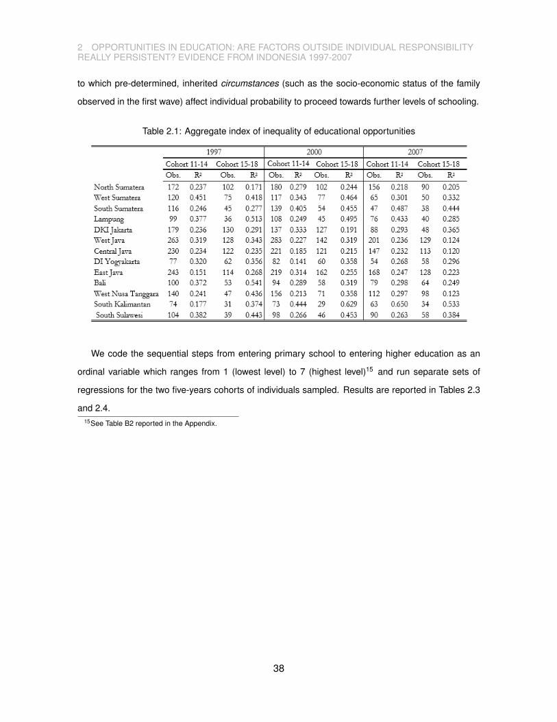
2 OPPORTUNITIES IN EDUCATION: ARE FACTORS OUTSIDE INDIVIDUAL RESPONSIBILITYREALLY PERSISTENT? EVIDENCE FROM INDONESIA 1997-2007
to which pre-determined, inherited circumstances (such as the socio-economic status of the family
observed in the first wave) affect individual probability to proceed towards further levels of schooling.
Table 2.1: Aggregate index of inequality of educational opportunities
We code the sequential steps from entering primary school to entering higher education as an
ordinal variable which ranges from 1 (lowest level) to 7 (highest level)15 and run separate sets of
regressions for the two five-years cohorts of individuals sampled. Results are reported in Tables 2.3
and 2.4.15See Table B2 reported in the Appendix.
38

2 OPPORTUNITIES IN EDUCATION: ARE FACTORS OUTSIDE INDIVIDUAL RESPONSIBILITYREALLY PERSISTENT? EVIDENCE FROM INDONESIA 1997-2007
Table 2.2: Decomposing inequality of educational opportunity into individual circumstances share
39

2 OPPORTUNITIES IN EDUCATION: ARE FACTORS OUTSIDE INDIVIDUAL RESPONSIBILITYREALLY PERSISTENT? EVIDENCE FROM INDONESIA 1997-2007
Table 2.3: Sequential Logit model for educational levels. Results for cohort 11-14
Our findings show that parental education positively influences school survival across most of the
levels of education. Among both cohorts of students, we observe that maternal education positively
affects the probability of being enrolled in senior high school and, for the oldest cohort, it is also
significantly associated (and with a relatively larger coefficient) with higher odds of proceeding towards
higher levels of education after graduation from high school.
Father’s education instead seems to positively affect the probability of both generations graduating
from primary school. It can be observed that the magnitude of these probabilities is always larger for
the youngest generations, which may imply that the importance of such a circumstance in driving
40
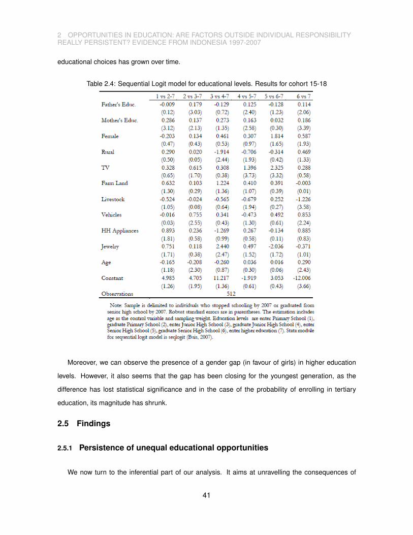
2 OPPORTUNITIES IN EDUCATION: ARE FACTORS OUTSIDE INDIVIDUAL RESPONSIBILITYREALLY PERSISTENT? EVIDENCE FROM INDONESIA 1997-2007
educational choices has grown over time.
Table 2.4: Sequential Logit model for educational levels. Results for cohort 15-18
Moreover, we can observe the presence of a gender gap (in favour of girls) in higher education
levels. However, it also seems that the gap has been closing for the youngest generation, as the
difference has lost statistical significance and in the case of the probability of enrolling in tertiary
education, its magnitude has shrunk.
2.5 Findings
2.5.1 Persistence of unequal educational opportunities
We now turn to the inferential part of our analysis. It aims at unravelling the consequences of
41
2 OPPORTUNITIES IN EDUCATION: ARE FACTORS OUTSIDE INDIVIDUAL RESPONSIBILITYREALLY PERSISTENT? EVIDENCE FROM INDONESIA 1997-2007
unequal opportunities in education because of exogenous pre-determined circumstances has on a
person’s future life outcomes.
Considering the distribution of young students’ rewards according to efforts and circumstances is
a very meaningful exercise in that it can tell how large a role pre-determined circumstances play in
influencing schooling opportunities ( given the limited responsibility of children that might have been
tolerated in the past) that persist over the individual life’s course.
By doing this, we can also get a clearer picture of the persistence or “stickiness” of the effects of
inherited circumstances and therefore their repercussions for intergenerational mobility. In particular,
we look at the effects in terms of future education achievement and of earnings on four different
cohorts of students ranging from the oldest ones, aged 15-18 in 1997 and aged 15-18 in 2000, to the
youngest ones, aged 11-14 in 1997 and aged 11-14 in 2000.
Panel A in Table 2.5 shows the results for the effects that inequality of educational opportunity
experienced in the past has on future school achievements (i.e. on the highest grade completed in
2007).
As discussed in Section 2.3, we measure the deviation of pre-determined circumstances in 2007
from its average over the periods of observation by the fitted values of the educational achievement
equation and, for the sake of interpretation, we normalize these fitted values in order to get an
index which goes from 0 to 100. The larger the value of this index, the stronger effect from the
latest circumstances on educational achievement relatively compared to those from the previous
circumstances, within each individual.
42

2 OPPORTUNITIES IN EDUCATION: ARE FACTORS OUTSIDE INDIVIDUAL RESPONSIBILITYREALLY PERSISTENT? EVIDENCE FROM INDONESIA 1997-2007
Table 2.5: Persistence in inequality of opportunity and future educational achievements
As these results suggest a significant cumulated and persistent effect of pre-determined circum-
stances seems to exist. The more educational opportunities that are granted to a person based on
her inherited circumstances, the larger her educational reward in the near future will be.
The coefficient on the effect of circumstances index indicates the difference between observation
with the lowest support of pre-determined circumstances during the last period compared to those of
the earlier periods (the standardized index of fitted values is 0) and the observations with the highest
ones (the standardized index of fitted values is 100) ranges from around 1.4 years for youngest cohort
aged 11-14 in 2000 to around 0.2 years for the oldest cohort (aged 15-18 in 1997).
One possible interpretation of the difference in the magnitude of the effect between the youngest
43

2 OPPORTUNITIES IN EDUCATION: ARE FACTORS OUTSIDE INDIVIDUAL RESPONSIBILITYREALLY PERSISTENT? EVIDENCE FROM INDONESIA 1997-2007
cohorts 11-14 and the oldest cohort15-18 is related to the fact that, due to their young age and
therefore lower maturity, young adolescents depend much more on the choices made by their parents.
Nevertheless, when comparing the coefficients for the youngest cohort measured in 2000 and the
one in the same age-range measured in 1997, our results also show that the current influence
of circumstances is stronger for the youngest generations, possibly implying that the distribution of
educational opportunities have become more concentrated over time.
On the other hand, for each of the cohorts under investigations the role of innate ability is relatively
larger than the power of circumstances and -when comparing the effect of the two youngest cohorts-
it has also grown over time.
Moreover, when considering the results in Panel B on the probability of enrolling in tertiary edu-
cation, we see that the indirect effect of current circumstances via education achievements is not at
all statistically significant for the two oldest cohorts. Conversely, among the youngest generations we
observe a positive and significant independent effect. Nevertheless, the effect of innate ability is not
only larger, but –as implied by the difference in the coefficients- has also grown relatively faster than
the effect of circumstances.
When looking at the results obtained from a simple Heckman model estimating the association
between earnings and the effect of circumstances index (see Table 2.6), one can also see that there
is a close and positive relationship between the role that latest circumstances played in the allocation
of educational rewards during adolescence and future earnings perspectives.
44

2 OPPORTUNITIES IN EDUCATION: ARE FACTORS OUTSIDE INDIVIDUAL RESPONSIBILITYREALLY PERSISTENT? EVIDENCE FROM INDONESIA 1997-2007
Table 2.6: Persistence in inequality of opportunity. Wage equations.
However, we see that in most of the cases the effect of current circumstances is not statistically
different from zero and relatively small in magnitude if compared to the effect of innate ability.
These results –that echo back to our previous results on tertiary education as well as our aggre-
gate figures on inequality of opportunity- imply that in our sample any “unfair” reward mechanisms at
school did not tend to persist and were not reflected in future earning perspectives.
2.5.2 Educational inequality of opportunity and public policy
Our next research question is whether educational budgeting policy has played a role in evening
the allocation of opportunities among the Indonesian students. We have observed that equality of
opportunity in education (as measured by the aggregate index at the province level as well as proxied
by the individual index of effect of the circumstances) has tended to improve slightly over time. Was
this improvement associated with an increase in the budget devoted to education?
In order to answer this question, we exploit the panel dimension of our data and estimate a fixed-
effects model relating the between-provinces variation in the budget share devoted to the education
45

2 OPPORTUNITIES IN EDUCATION: ARE FACTORS OUTSIDE INDIVIDUAL RESPONSIBILITYREALLY PERSISTENT? EVIDENCE FROM INDONESIA 1997-2007
sector to the between-province variation in inequality of opportunity, as measured by our effect of
circumstances indices obtained for the cohorts 11-14 and 15-18.
The results, which are reported in Table 2.7, show that while one of the oldest cohorts has
experienced better pro equality policies, there is a more stable, positive and significant relationship
between inequality of opportunity and spending in education when considering the results obtained
for the youngest cohort.
These findings may be interpreted as such despite the differences in the way financial resources
have been spent over time.
The oldest cohort of students, aged 15-18 in 2000, seems to have benefited extensively from
various supply side interventions, targeting especially secondary school (such as the realignment of
the education system and the creation of new vocational schools) that were realized in the aftermath
of the 1997 crisis. By simply increasing and diversifying the supply of education, these policies
created more opportunities for secondary school students to achieve higher education levels. At the
same time, the campaign concerning the benefits of studying at vocational schools to increase the
demand side has also been actively taking place. Students or households that have no intention of
obtaining tertiary education were advised to attend vocational schools, since this schooling type has
a lower opportunity cost as the skillful fresh graduates are more ready to enter the job market than
the traditional high school graduates.
On the other hand, the effectiveness of the allocation of provincial budgets to primary and junior
high schools has been more ambiguous: more resources were devoted to hire a greater number of
teachers, assigning each teacher to teach one subject and therefore decreasing the students/teachers
ratios. Yet –as remarked in various reports (Suryadarma and Jones, 2013; OECD and Asian Devel-
opment Bank, 2015) - this mechanism has been highly inefficient, especially for small schools that
are mostly located in remote and disadvantaged areas where problems related to teachers’ lack of
motivation and absenteeism were more frequently observed.
46
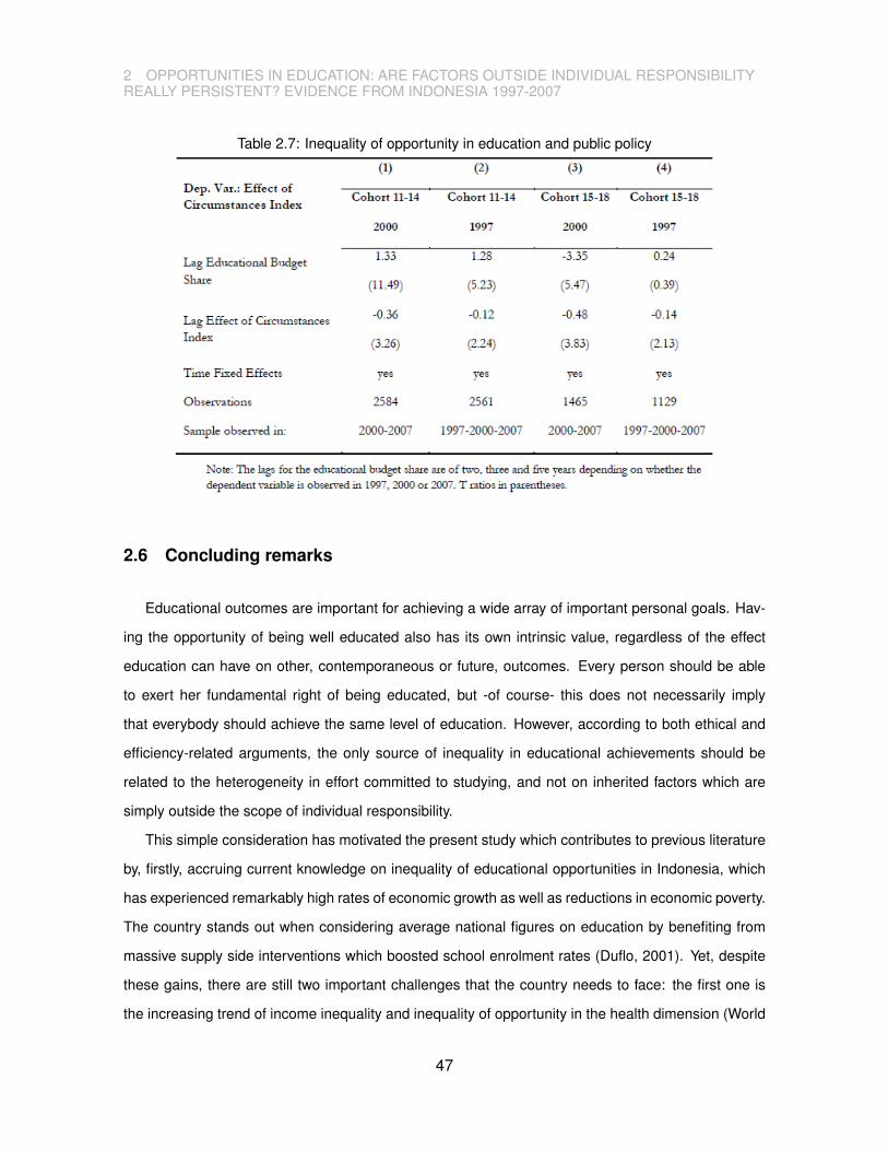
2 OPPORTUNITIES IN EDUCATION: ARE FACTORS OUTSIDE INDIVIDUAL RESPONSIBILITYREALLY PERSISTENT? EVIDENCE FROM INDONESIA 1997-2007
Table 2.7: Inequality of opportunity in education and public policy
2.6 Concluding remarks
Educational outcomes are important for achieving a wide array of important personal goals. Hav-
ing the opportunity of being well educated also has its own intrinsic value, regardless of the effect
education can have on other, contemporaneous or future, outcomes. Every person should be able
to exert her fundamental right of being educated, but -of course- this does not necessarily imply
that everybody should achieve the same level of education. However, according to both ethical and
efficiency-related arguments, the only source of inequality in educational achievements should be
related to the heterogeneity in effort committed to studying, and not on inherited factors which are
simply outside the scope of individual responsibility.
This simple consideration has motivated the present study which contributes to previous literature
by, firstly, accruing current knowledge on inequality of educational opportunities in Indonesia, which
has experienced remarkably high rates of economic growth as well as reductions in economic poverty.
The country stands out when considering average national figures on education by benefiting from
massive supply side interventions which boosted school enrolment rates (Duflo, 2001). Yet, despite
these gains, there are still two important challenges that the country needs to face: the first one is
the increasing trend of income inequality and inequality of opportunity in the health dimension (World
47

2 OPPORTUNITIES IN EDUCATION: ARE FACTORS OUTSIDE INDIVIDUAL RESPONSIBILITYREALLY PERSISTENT? EVIDENCE FROM INDONESIA 1997-2007
Bank, 2014)and the other one related to large disparities within and between provinces and regions
in many quantitative and qualitative indicators of school achievement (World Bank, 2011; OECD and
Asian Development Bank, 2015).
Second, we identified the factors (or “circumstances”) that account most for overall inequality of
educational opportunity and found that parental educational background is one of the most important
pre-determined circumstances that affect educational inequality of opportunity.
We contribute to previous literature on this field by devising an “individual” index of the effect of
circumstances, which is given by the fitted values representing the importance that, for each individ-
ual, the deviation of current circumstances from its average have on her educational achievement.
By using this index we were able to show how persistent these circumstances are over the individual
life’s course and thus how relentless current levels of inequality of opportunities are.
We also observe for the youngest cohorts a positive trend between inequality indices and educa-
tional budget share. This evidence may suggest that the increase in the educational budget share
has not been efficient and has led to an increase in inequality.
48

3 THE IMPACT ANALYSIS OF FUEL SUBSIDY REDUCTION COMPENSATION PROGRAM ONEDUCATION IN INDONESIA: THE BKM AND THE BOS
3 The Impact Analysis of Fuel Subsidy Reduction Compensa-tion Program on Education in Indonesia: the BKM and theBOS
Abstract
In this paper, we evaluate the short run impact of two educational subsidies that were part of the
fuel subsidy reduction compensation programs in Indonesia during the 2006/2007 academic year,
namely BKM scholarships and BOS out-of-pocket expenses, on education outcomes and household
expenditure. These are two different poverty-based targeting transfer programs that have been
represented by one single treatment variable in our data source, the Indonesian Family Life Survey
(IFLS), thus the clear identification of each program is very important to the disentanglement of
the estimated effects. The evalution becomes complicated because there is an effect of the past
scholarship program to be considered, as well as overlapping periods of two interventions and the
presence of BOS in the higher hierarchy as the school focused intervention at the same time. Utilizing
the combination of several methods, we find that targeting the poor was done inefficiently and that
the transfer coverage was too small. In addition, we find that educational attainment increases, on
average, by 4 months after one year of intervention for compulsory grades 1-9. This magnitude,
however, is an upper bound of the effect of intervention accumulation over time and is most likely
coming from the BOS spillover effect. We also observe crowding out household expenditure to
anticipate the transfers. Finally, we find a positive relationship between past scholarship programs
and educational attainment, which suggests that targeted subsidies also have a long term impact.
Based on a joint work with Stephan Klasen and Inmaculada Martinez-Zarzoso.
49
3 THE IMPACT ANALYSIS OF FUEL SUBSIDY REDUCTION COMPENSATION PROGRAM ONEDUCATION IN INDONESIA: THE BKM AND THE BOS
3.1 Introduction
Monetary interventions on education have been a part of development programs in many coun-
tries. They are often a way for the developing countries, which often do not provide adequate
resources to struggling households, to send their children to school. Typically, the government is
expected to redistribute income through subsidies to poor children so that the lowest stratum of the
society also has access to education. An alternative is often a universal subsidy where all children
get similar benefits from the intervention.
There is a lot of literature on impact evaluations in education. These studies give us a better
understanding of and the areas where interventions had a significant impact on education outcomes
and what exactly was done. The mixed evidence suggests, however, that more studies are required to
capture more dimensions of the interventions and to provide a clearer picture, including the dynamic
relationship between the cash transfer and household expenditure in education.
The motivation of our study in Indonesia is very much related to the spirit above. After the Asian
financial crisis in 1997, education subsidies to poor households was introduced to retain school
attendance under a big umbrella of Jaringan Pengaman Sosial (JPS) program. The JPS scholarship
phased out after 5 years and was replaced by Bantuan Khusus Murid (BKM), a similar program
that targeted poor households. More educational subsidies continued in the following periods, while
comprehensive assessments on the impact of the previous programs were not adequate1. This
hindrance was noticed by Jimenez and Patrinos (2008), who stated that the problems that usually
follow the expansion of the intervention stem from a lack of knowledge concerning the subsidies’
marginal advantage.
Our contribution to this topic is complementing and expanding the literature on the impact of
educational subsidies in Indonesia through identifying the impact sizes and discussing the sources
of suboptimal outcomes of the cash transfer program dedicated to education given in the 1996/1997
academic year. The assistance includes BKM scholarship and out-of-pocket expense from BOS grant.
We also include limited assessment of the impact of school grant on the outcomes.
The paper is organized as follows. Section 3.2 includes the literature review exploring the empirical
evidence on financing education and impact studies, as well as description of the interventions. We
1The existing impact studies for BOS i.e. Sparrow (2007) and Cameron (2009); for JPS, World Bank (2007; 2009), Al-Samarrai et al. (2014).
50

3 THE IMPACT ANALYSIS OF FUEL SUBSIDY REDUCTION COMPENSATION PROGRAM ONEDUCATION IN INDONESIA: THE BKM AND THE BOS
discuss data and methodology in Section 3.3. Section 3.4 focuses on the results while conclusion
and policy implications are given in Section 3.5.
3.2 Literature Review
3.2.1 Financing education and impact evaluations at a glance
Developing countries usually have financial restrictions when they determine the priority budget
for development, and to an extent for education. This limitation could be different across countries.
The most effective strategy to expand access and improve the quality of education thus depends on
the specific profiles of the country. For instance, there has been much debate regarding whether
financing education should be the full responsibility of government or if households should have a
higher level of participation.
On the one hand, the argument in favor of user fee introduction is reasonable when the supply
side is unsatisfied, i.e. there has been years of underinvestment and neglect of the public educa-
tion system, and user payment is expected to improve the quality of the teaching-learning process.
Students are definitely better off with this system when free public education does not exist, but it
loses substance when the problem is on the demand side. One example of user fee case is in Chad,
where paying the schooling fee was the only option left for the children because high demand existed
even from the poorest households, yet it was not accompanied by the supply side. Children would
be worse-off if that choice is unavailable (Jenkner and Hillman, 2002). A user fee for compulsory
education, however, is similar to a regressive tax. Eventually it burdens the poorest group of the
society since the cost of schooling is fixed. Moreover, relying on private financing is not sustainable
and will in the end produce higher inequality through a more exclusive schooling system because
school fees are a barrier to education (see Kattan and Burnett 2004; World Bank and UNICEF 2009).
On the other hand, arguing that public spending should finance education has more rational
grounds, as long as the taxation system is progressive (Jimenez, 1986). It is an effective mean
of income distribution that fulfills the equity principle. Additionaly, externalities, scale of economics
and market imperfection defend public spending reasoning from the efficiency perspective. Hence,
intervention through financial subsidies to education is relevant provided that full financing system for
education is not an option. In developing countries with suboptimal progressive tax, nevertheless,
51

3 THE IMPACT ANALYSIS OF FUEL SUBSIDY REDUCTION COMPENSATION PROGRAM ONEDUCATION IN INDONESIA: THE BKM AND THE BOS
equity gets away and it is worse if the spending type is regressive, i.e. university absorbs the
largest part of the subsidy. Meanwhile, inefficiency occurs when the resources are misallocated,
such as when the wrong students are selected to receive the subsidy or no incentive is provided for
the administrators to allocate the subsidy fairly. Inefficiency during the intervention will slower the
implementation and eventually degrade the benefits Jimenez and Patrinos (2008). Those barriers
make difficult to see the potential impact of the interventions.
Suboptimal outcomes in educational performance given the intervenstions is not a good news. The
policies will be seen as ineffective by political opponents: thus future budgets might move into other
areas. Education is a long term investment and unnecessary distraction concerning the financing
system should be avoided at all cost. A reliable assessment through a series of impact studies would
be beneficial in providing a framework of understanding what needs to be improved.
There has been a lot of impact evaluation research concerning interventions in education. The
reviews can be found in the studies from i.e. Glewwe and Muralidharan (2015), Evans and Popova
(2015), Conn (2014), Glewwe et al. (2013), Kremer et al. (2013), Krishnaratne et al. (2013), Masino
and Niño-Zarazúa (2015), McEwan (2015), Asim et al. (2015), and Murname and Ganimian (2014).
The large body of literature suggests mixed findings for the impact of monetary intervention. For in-
stance, providing free education indiscriminately has an overall positive impact on education (Bhalotra
et al., 2014). In addition to this, reducing transportation costs from home to school has a positive
effect on attendance and attainment (Murname and Ganimian, 2014). Yet, evidence from Malawi and
Uganda reveals that universal intervention where fees are abolished and more classrooms are built,
shrinks the quality of education (Jenkner and Hillman, 2002).
Interventions can also have an impact on household expenditure. Das (2004) utilizes the maxi-
mization approach to evaluate the impact of government subsidies on inequality in educational expen-
diture. His study from rural Zambia shows that when the cash is allocated with clear guidance and
rules, and when the implementation considers the distribution of wealth within and across different
schools, the second best approach was successful in reaching the correct schools. However, even
when the grant distribution was highly progressive, it failed to act as an equalizing transfer since it
crowded out household spending at all levels and the extent of substitution was greatest among the
poor. There is also no significant association between the size of the subsidy and the beneficial
outcomes. Concerning the learning outcomes, Das et al. (2002) find that cash grants have no impact
on learning outcomes.
52

3 THE IMPACT ANALYSIS OF FUEL SUBSIDY REDUCTION COMPENSATION PROGRAM ONEDUCATION IN INDONESIA: THE BKM AND THE BOS
After learning from other studies, we shift our attention to Indonesia, which after the 1997 Asian
financial crisis started paying more attention to education and released several subsidy policies in
order to improve human capital even though it was and has been constrained by a tight development
budget. Among the various types of interventions, our study has largely focuses on conditional trans-
fers. This is a supply side type of intervention targeting households, as the transfers are conditioned
on the households’ children attending school. It aims at equity in order to provide free education to
the poorest group, even though it does not dismiss the high opportunity cost factor. Another type of
intervention included in our study is creating a demand for schooling by improving access and school
quality through school grants. This is a universal subsidy that considers the positive externalities of
education, in that the whole society is better off when people are educated.
3.2.2 Country context: Indonesia
Public education in Indonesia normally charges a user fee, even though it is generally less expen-
sive than those of the private schools. During the Asian financial crisis in 1997, many people suffered
from economic turbulence. The Jaringan Pengaman Sosial program (JPS) was therefore launched to
the population overcome the negative impacts of the crisis that increased the number of poor people
quickly. One of the targeted areas was education, where a scholarship program was established
to cover the fees of millions of students in order to retain school participation (see Sparrow 2007
and Cameron 2009 for the impact studies). The program, however, ended after five years and was
completely replaced by a similar type of program with a simplified delivery system called Bantuan
Khusus Murid (BKM) that started in 2001 following the initial increase of fuel domestic price.
Four years later, another subsidy program at the school level, named Bantuan Operasional Seko-
lah (BOS) as the part of the second fuel subsidy reducation compensation program, was introduced.
How large the marginal impact of those interventions was remains unclear when the next subsidies
were released2. In order to complement other studies, we contribute to this part of literature by eval-
uating the impact of both programs on education outcomes and household spending on education.
Our interest is specifically on the impact of cash transfers on households, yet the impact of grant to
school is provided as comparison and to test its spillover effects. We also discuss the possible source
of suboptimal outcomes and how they could be improved.2Such as Bantuan Siswa Miskin (BSM), Beasiswa Bidik Misi, Kartu Indonesia Pintar (KIP).
53

3 THE IMPACT ANALYSIS OF FUEL SUBSIDY REDUCTION COMPENSATION PROGRAM ONEDUCATION IN INDONESIA: THE BKM AND THE BOS
Figure 3.1: Timeline of education subsidies
The timeline of the educational assistance program is presented in Figure 3.1, showing the three
programs that overlap each other. This fact is both an important feature as well as a critical barrier
of this study, since a clear identification is required to measure the marginal effect of the concerned
programs. The next sections investigate the backgrounds of the BKM and the BOS programs. We
also explain how to cover the JPS scholarship, which is not the target of this study but acts as the
confounding, in the methodology section.
The BKM
The reduction of fuel subsidies in 2001 was the main motivation behind launching the scholarship
programs BKM or Students Special Assistance, which was the complement of the JPS scholarship
whose purpose was to extend the coverage of financing basic and secondary education. Fuel subsidy
reductions trigger volatility of the basic food prices and erodes household expenditure. Poor house-
holds most likely dealt with the situation by reducing non-basic expenditures to survive, including
decreasing their the investment in education. Hence, students from these households would have
been the most vulnerable ones. Scholarships such as the BKM were launched to help them stay in
school during the crisis. BKM was therefore the main policy (together with JPS scholarship until it
ended in 2003) that kept children in school. It started in 2001 and the fund was from the savings of
fuel subsidies reduction. The semester allowance for primary school students was about 6.25 USD,
for junior secondary school students the number was double and for senior secondary students it was
more than double.
The mechanism and allocation of BKM funds follow the principles of decentralization where the
poverty index, the number of student and the number of schools determine how much is allocated to
each district (kabupaten/kota). The district committee distributes the funds to schools after receiving
54

3 THE IMPACT ANALYSIS OF FUEL SUBSIDY REDUCTION COMPENSATION PROGRAM ONEDUCATION IN INDONESIA: THE BKM AND THE BOS
the list of the approved nominees. To become a BKM beneficiary, which was determined at school
level, was similar to the previous JPS program and somewhat flexible. It considers of socio economic
background of the family, dropping out history, the distance from home to school, the number of
siblings under 18 years old at least three persons, and if the nominee is an orphan. A gender based
rule also applies as at least 50 percent of the participants have to be girls.
Kompas Daily (2011) reported that in the first semester the total number of participants for the
BKM program was 5,075,000 students. In the same article, it cited a high profile official who indicated
that the mechanism used to select the correct beneficiaries was too much work for the committees at
the school and district levels since the time frame provided for the selection was quite short, and they
had to select beneficiaries from tens of millions of students. The following period, the take up rate was
nearly 20 percent for primary school students and 26 percent for junior secondary students in 2004
(Hardjono et al., 2010). Finally in 2006, the number of recipients was 8,283,200 (SMERU, 2006).
BKM gradually phased out after the Schools Operational Assistance (BOS) program was introduced
and it ended entirely in 2011.
Before BKM was introduced, JPS was used to cover students grade 5-12. When BKM was
introduced, the first year covered grade 1-4 to complement JPS. However, it covered all grades in
the second year and continued to do so until BOS was launched. As BOS was being a universal
subsidiy for compulsory grade3, BKM then covered only for grade 10-12.
To the best of our knowledge, a rigorous impact study of this program is not identifiable. A study
from SMERU (2003), however, suggests that this program was not designed with a good monitoring
system and lacked of long-term financial planning. Surprisingly, they do not find leakage as a serious
problem, which is contrary to the finding on the JPS scholarship from Sparrow (2007) .
The BOS
The second phase of fuel subsidy reduction occurred in 2005. The government implemented a
similar policy to prevent students from leaving schools by allocating part of the savings from the fuel
subsidies reduction for education. This time, the recipients shifted from households to schools and
was entitled the Bantuan Operasional Sekolah (BOS). The main aim of this program was to improve
the quality of the schools and achieve better education outcomes. There was operational assistance3BOS started to cover senior secondary level only since the 2013/2014 academic year.
55

3 THE IMPACT ANALYSIS OF FUEL SUBSIDY REDUCTION COMPENSATION PROGRAM ONEDUCATION IN INDONESIA: THE BKM AND THE BOS
for schools prior BOS was implemented. However, BOS coverage was much wider and school
involvement in BOS was not appointed, rather it was on voluntarily basis and called for applications.
This program depended on public participation to ensure transparency through the involvement of
parents and school committees in making decision about how the grant was used. This rule shows
how an effort was made to keep the project on the right track. Good governance is an important key
successfully to managing large financing programs in education, as demonstrated by Rajkumar and
Swaroop (2008) in their study about how public spending on primary education can increase primary
education attainment. Literature that endorses community involvement in designing projects includes
Khwaja (2009) and Reinikka and Svensson (2002). This argument is the part of a larger study on aid
effectiveness, which argues that the role of institutions matters (see Acemoglu et al. 2001; Burnside
and Dollar 2000; Frye and Shleifer 1997; Djankov et al. 2002).
The number of students becomes the basis for determining the amount that is transfered to
schools. This means, schools with higher number of students obtain a higher amount of funding.
The capita grant assigned for each primary school student per semester in 2006 was US$ 24.21 and
US$ 33.44 for every junior secondary school student (Government of Indonesia, 2011). According
to the BOS Guideline Book 2006, the goal of BOS was to provide free education for poor students
and to reduce education costs for other students, in order for students to acquire a better quality of
basic education and be able to complete it4 (SMERU, 2006). The average growth of the BOS budget
was 32.7 percent per year, and in 2010 the World Bank agreed to financing this program under the
name School Operational Assistance-Knowledge Improvement for Transparency and Accountability
(BOS-KITA) (Government of Indonesia, 2011).
The number of participants that attended BOS schools in 2006 was 39,700,000 with the grant
amount totaling was IRD 9,900 billion, which is equals to about USD 1,1 billion (ILO, 2015). The
guidelines specified for how the BOS grant should be spent including abolishing regular fees, paying
for school supplies, maintenance and monthly bills, remunerating local teachers and staffs, training
teachers and compensating for students activities5. In addition to this, schools were allowed to directly
send some money to poor students to compensate them for their transportation cost. Contrarily, there
was also a room to charge students if schools found that their total expenditure exceeded the grant.
School heterogeneity i.e. no standardized expenditure, made the amount of money charged to each
4Completing 9 years compulsory education.5 see Table C1 in the Appendix for complete description
56
3 THE IMPACT ANALYSIS OF FUEL SUBSIDY REDUCTION COMPENSATION PROGRAM ONEDUCATION IN INDONESIA: THE BKM AND THE BOS
student largely vary across different schools6. The only strict exception was for students who were
identified as being from poor households. In that case, schools were not allowed to charge them,
regardless of the decision made for other students. The definition of poor students, however, was not
strictly defined as was the case for the BKM program. Only occasionally schools require a certificate
from a village official explaining that the students were from an impoverished background (SMERU,
2006).
A field study from SMERU (2006) finds that only 47 percent of their school sample actually sent
the transfer to poor students, which is around 6.5 percent of total students, or equal to 22 percent of
poor students. The expenditure for poor students was quite low and was usually not within the top
five expenditures. They also observe that rich private schools tended to reject BOS grant.
The fraction of school that rejected the grant was less than 5 percent. The main reason behind
this was that the rules that had to be obeyed were too much. The fees from the wealthy students
covered everything and it was enough to maintain school independency. This is a strong incentive to
reject BOS.
Meanwhile, World Bank (2009) indicates that schools tended to use BOS funds for teacher hon-
orarium instead of on poor students. Moreover, although community involvement was enforced to
support the transparency, they suggest that most schools participating in the grants ignored this party
when making the allocation decisions. Additionally, Indonesian Corruption Watch (ICW) estimates
that BOS only treated 30-40 percent of operational schools, which is significantly lower than the
calculation from the Ministry of Education which claimed it to be about 70 percent (Kontan, 2010).
Massive allocation of public spending with improper supervision eventually leads to potential
misuse, as reported from national and local newspapers. ICW indicated two points of BOS implemen-
tation that required higher levels of supervision when money is transferred from districts to schools
and when there is hidden business being done using BOS funding. Several schools bribed districts
officials to ease the transfer process, while the hidden businesses were created when schools printed
mandatory worksheets for students and charged the expenditure to BOS (Kontan, 2010). Another
source of leakage through the headmasters, as they are the only authority at school. This is twice
as problematic, as having a single decision maker violated the regulation that required not only public
participation but additional teacher involvement in decision making and management as well. But the
lack of strict monitoring system allowed for this practice.
6In some areas local authorities also played an important role in deciding whether they would allow schools to charge thehouseholds of students if schools received the grant.
57
3 THE IMPACT ANALYSIS OF FUEL SUBSIDY REDUCTION COMPENSATION PROGRAM ONEDUCATION IN INDONESIA: THE BKM AND THE BOS
ICW reported that the estimation of BOS grant manipulation calculation by Indonesian Supreme
Audit Board in 2007 and 2008 for 3.237 schools was nearly 3 million USD with the average misap-
propriation for each school being around 1,450 USD. They observed only 36.5 percent of schools
were free from the grant misuse. Moreover, there are 33 cases of corruptions related to BOS during
2004-2009 with the estimated loss of nearly 1.4 million USD. School principals as well as the heads
and staffs of district education offices were suspected as the culprits (Kompas Daily, 2011).
Since the grant did not demand a good performance to be given, another form of misuse might
have taken place, such as inflating the number of pupils in order to attain a larger grant. During
this period, the student database was not accurate thus was able to ease this practice. However,
if schools inflated the number of students in the BOS proposal to anticipate a higher number of
previously predicted new students for the next academic year, they were able to make adjustments in
the following phase.
World Bank (2007)suggests it is hard to assess the actual impact of the grant because a demand
for achievement did not exist and there was a lack of transparency. However, they manage to attain
some findings through the correlation of the grant with the growing number of students from poor
households that were being enrolled, even though this effect was temporary. They also find that the
initial phase of the BOS implementation is associated with 6 percent drop of annual education spend-
ing for households. This figure is relatively low compared to the per capita BOS grant allocated to
students through the schools. The reduction is found to be from students from the poorest households
and from students who attended government schools. After schools became familiar with BOS, the
spending gradually increased again.
In addition, they notice that schools boosted the number of non-civil servant teachers up by 50
percent after the BOS grant was launched7. The impact on transition rates from primary to secondary
education was also temporary, and there was no significant jump after increasing the amount of the
grant . The BOS grant is also associated with the initial decline in educational spending for primary
and junior secondary students. They suspect that low level of public participation in determining how
the BOS was used is the key answer behind those suboptimal returns. Another reason is that other
financing resources dropped after BOS policy was introduced. Whereas, the use of BOS has been
limited and strictly regulated that creates difficult situation for schools who had to balance their typical
needs that were not listed in the BOS coverage (Al-Samarrai et al., 2014). Additional evidence from7For government schools, there was a limitation of spending 10 to 20 percent for teachers honorarium
58
3 THE IMPACT ANALYSIS OF FUEL SUBSIDY REDUCTION COMPENSATION PROGRAM ONEDUCATION IN INDONESIA: THE BKM AND THE BOS
Kharisma (2013) suggests that there was no significant impact of BOS on dropout rates for students
age 7-15. Therefore, in general the BOS program seems to have done less to expand access to
education and improve quality than its true capacity.
3.3 Data and methodology
3.3.1 Data
Our data is Indonesian Family Life Survey (IFLS). This survey contains four completed waves, i.e.
1993, 1997, 2000 and 2007. As BKM was firstly introduced in 2001 and BOS started in 2005, we
use the observation in 2000 to capture the information before the intervention, i.e. BKM or BOS (see
Methodology for the precise definition of the intervention). Furthermore, IFLS records the response
of the intervention in 2006/2007 academic year89. Therefore, the observation in 2007 can reveal the
impact of this intervention, with the possibility of capturing the effect of the previous interventions in
2001-2005 that were not registered by the survey.
IFLS is known to have rich information on the socio-demographic of households: information that
is closely related to some eligibility rules and traditional covariates. More specifically, we are able
to link the parental information on the educational attainment to the children’s information in order to
control for the intergenerational mobility persistence. There are three levels of education: primary
(grade 1-6), junior secondary (grade 7-9) and senior secondary (grade 10-12). For further discussion,
we use the term level and grade interchangeably. Since the reported transfer was in the 2006/2007
academic year, the BKM scholarship was specifically for grades 10-12, while out-of-pocket expenses
from BOS was for the compulsory grades 1-9.
Our main sample is from the post treatment period in 2007. It is limited to students that were
at school in 2006/2007 academic year so it remained eligible for the transfer10. We also ignore
households that reported that their educational expenditure exceeded 30 percent11. Moreover, there8We assign the observation as getting exposed to the intervention if the respondents stated they received the transfer. This
group consists of two subgroups: those who could report the amount of the assistance and those who could not. We employthe subgroup analysis for robustness check and find that results from the overall sample is more similar to those from subgroupthat reported the amount of the assistance. Results of subgroups are not shown.
9see Table C1 in the Appendix for the complete questionnaire10If students drop out or stop attending school during the transition period, the school can list them as a nominee, conditioned
on their coming back to school (source: the annual BOS Guidance Book).11Our exploratory analysis suggests that household educational expenditure that is larger than 30 percent seems to be
outlier. Moreover, this number is too high that makes it unlikely to happen. One possibility of this case is measurement errorswas occured during the survey.
59

3 THE IMPACT ANALYSIS OF FUEL SUBSIDY REDUCTION COMPENSATION PROGRAM ONEDUCATION IN INDONESIA: THE BKM AND THE BOS
is information at the school level for a limited number of observation in the survey. Hence, we are able
to link this information to some students to assess the spillover effects of BOS school grant12.
3.3.2 Methodology
In this paper, we propose the combination of several methods to evaluate the targeting practice
and the impact of the intervention on the outcomes of interest. Our intervention is defined as the cash
transfer sent to households from the BKM program or the out-of-pocket expense from the BOS grant
sent from schools to households, depended on the grade, in 2006/2007 academic year. Furthermore,
we focus on evaluating the impact of this intervention on two outcomes, educational performance
and household expenditure. Educational performance includes cognitive test scores and educational
attainment. Cognitive test scores are not available for the entire sample since the tests were assigned
to selected students. Educational attainment is calculated by combining the reported level and
the highest grade attended, i.e. junior secondary school at the second grade equals to grade 8,
although the actual years of schooling might be longer, or in a very rare cases shorter by means
of an acceleration program. The impact on household expenditure is measured by the share of the
household’s expenditures that is spent on education.
We analyze the impact with two different approaches. The first one is using cross sectional
information to assess the association between the intervention and the outcomes, while at the same
time controlling for other factors. Our preliminary analysis indicates that for the education outcomes,
namely cognitive test scores and educational attainment, the intervention is not proved to be endoge-
nous13. This is a feasible perspective since the selection process does not include education-related
outcomes as the basis of choosing participants. We thus argue that assistance is an exogenous
treatment variable for these outcomes. Assistance is nevertheless most likely to be endogenous when
outcomes are highly correlated with economic variables. Consequently, to model the association with
learning outcomes we will use a simple framework such as ordinary least square for cognitive test
scores and a poisson regression for educational attainment. The utilization of an instrumental variable
model is additionally required to deal with endogeneity of household educational spending.
The second approach is done by employing panel data to examine the differences in outcomes
before and after the intervention. The difference-in-difference method removes the fixed differences12 All variables and their descriptive statistics are presented in Table C3 in the Appendix.13This is a robust case, as endogeneity test is insignificant and statistics lambda from the treatment effect model also
suggests that selectivity is insignificant.
60
3 THE IMPACT ANALYSIS OF FUEL SUBSIDY REDUCTION COMPENSATION PROGRAM ONEDUCATION IN INDONESIA: THE BKM AND THE BOS
between the control and treated groups over time, so that what is left is expected to be the rel-
atively pure effect of the treatment after controlling for several confoundings i.e. gender dummy,
residential dummy, repetition dummy, educational level, parental educational attainment and province
fixed effects. This approach is enhanced by propensity score matching to provide a counterfactual
observation.
In addition to this, we use sampling weights in the inferential analysis to reduce sampling bias.
Our robustness check, done by comparing goodness of fit of tests between models with and without
sampling weights, suggests that models with sampling weights have in general better fittings14.
Finally, we need to emphasize that we measure the marginal effects of the transfers under the
assumption that other factors, including household spending, does not anticipate the transfer by
making adjustment. If this assumption does not hold, the actual impact will potentially be different
and parameter adjustments should be made, which is beyond the scope of the study.
Formal model
Our general model for the impact study using cross-section information is
Yi = γWi + βXi + εi, i = 1, ...N (3.1)
Yi is the outcome variables of individual i, Wi is the dummy variable, taking the value 1 if individual
i gets the assistance and zero otherwise, Xi is a set of exogenous control variables that determine
the outcomes Yi. If assistance is exogenous, then this model translates into linear regression for the
outcome cognitive test score; and poisson regression for educational attainment.
Whereas, the assistance variable W might be endogenous for educational spending outcome,
because the eligibility rules are pretty much related with socio-economic background and those could
have affected the decision about whom deserved the transfer. The formal form of this relationship is
E(W, ε) 6= 0. If this is the case, γ is not a consistent estimator in OLS model. Our strategy is to use
14We assess the goodness of fit by using Root Mean Squared Errors (MSE) for linear regression and log pseudo likelihoodfor Poisson regression. We find that models with weights outperform models without weigths in regression analysis moreoften. Furthermore, log pseudolikelihood is always bigger for Poisson regression with weights compared to the non weightscounterpart. In IV model, the issue of goodness of fit is more relevant to the first stage regression, that is whether endogeneityis a real problem. The same sample shows that p-values of endogeneity tests for models with weights are smaller in mostcases. It indicates that excluding weights might be correlated with the lower power to detect endogeneity. We wrap this part byconcluding that for our sample it is preferable to employing models with weights and the interpretation of the results follow thesame manner. Results without weights are not shown here.
61
3 THE IMPACT ANALYSIS OF FUEL SUBSIDY REDUCTION COMPENSATION PROGRAM ONEDUCATION IN INDONESIA: THE BKM AND THE BOS
the Instrumental Variable (IV) model to deal with endogeneity by replacing the actual realized values
of W with different values that correlate the with actual W and are at the same time uncorrelated with
ε conditioned on all other covariates X. Let us call this variable Z.
The linear projection of Z on W
Wi = πZi + µi, i = 1, ...N (3.2)
We require that E(Z, ε) = 0. Moreover, the estimated coefficient shall be π 6= 0. If we can find
such variables, our instruments are valid and informative. Moreover,
Wi = πZi + µi, (3.3)
where Wi is a latent endogenous variable, Zi is a vector of exogenous variables to predict the
selection outcome Wi, Φ(o) is the standard normal cumulative distribution function, εi and µi are
bivariate normal with mean zero and covariance matrix
σε ρ
ρ 1
. The IV model considers W in
equation 3.3 as the direct replacement of W in such the outcome regression for the IV model is
Yi = γWi + βXi + εi, i = 1, ...N (3.4)
Whereas, difference in difference method with the pre-treatment covariates has a formal model as
follow:
Yi = β0 + β1.periodi + β2.treatedi + β3.periodi.treatedi + βk.Xk,i + εi, i = 1, ...N (3.5)
where period is a dummy variable indicating the baseline or before the treatment given, if period is
zero (i.e. year 2000), and the follow-up, or after the treatment given, if period is one (i.e. year 2007),
treated is a dummy variable zero or one, indicating the control and the treated group, consecutively.β3
is the DiD or the impact and Xk,i is the kth covariate of individual i.
62

3 THE IMPACT ANALYSIS OF FUEL SUBSIDY REDUCTION COMPENSATION PROGRAM ONEDUCATION IN INDONESIA: THE BKM AND THE BOS
Propensity score matching is another method in impact evaluation that provides a counterfactual
observation from statistical matching that accounts for the covariates which predict receiving the
treatment (see Guo and Fraser 2014). The simple comparison between outcomes of the treated and
outcomes of the non-treated is based on a substantial overlap between the two groups. The common
supports in the matching in order to meet the overlapping assumption are household wealth index
and if they are exposed to JPS scholarship period. The latter variable is defined as “high” to indicate
that observations with the value one get assistance with a higher intensity rate throughout their basic
and secondary educational periods. It is unknown if they truly received the JPS scholarship. This
variable thus reflects only the possibility of receiving the treatment or the spillover effect.
Our final approach is the combination of both methods to present estimates that can simultane-
ously reduce the confounding bias as well as remove fixed differences between the two groups. Since
the Rubin causal model is applied, we argue that results from this approach has a stronger causal
interpretation15.
The instruments
To find an instrument that is only correlated with the endogenous variable and not with other
predictors is challenging in most cases. We consider two instruments in our models. The first one is
an individual mistargeting dummy. To produce this variable, we regress three eligibility requirements
in vector X against the transfer dummy W using probit model as in equation 3.6.
W = βX + ε,∼ N(0, 1)⇒ W = βX (3.6)
W =
1 if W>0
0 otherwise
W is the linear prediction, W is the binary predicted value, X is the a vector of explanatories that
defines the formal eligibility rules. The eligibility rules in this model are a wealth index, orphan dummy
and dummy for when the number of siblings under 18 is more than 2. Other eligibility rules are not
15Additionally, we use a Gaussian kernel density and bootstrap of 1000 replications to provide a more precise estimation ofthe matching.
63
3 THE IMPACT ANALYSIS OF FUEL SUBSIDY REDUCTION COMPENSATION PROGRAM ONEDUCATION IN INDONESIA: THE BKM AND THE BOS
included in the model for several reasons, i.e. the information on the distance between the home and
school is unavailable, whereas disruption predicts one of the outcome categories perfectly.
The predicted values W are cross-checked with the original values W as expressed in equation
3.7 to determine M , the dummy of mistargeting. We assign M as having the value of 1 if predicted
and original are different, 0 otherwise.
M =
1 if W 6= W
0 if W = W
(3.7)
It is clear from equation 3.6 and 3.7 that M is highly correlated with W . However, M is less likely
to correlate with the outcomes.
To add randomness, we introduce the second instrument. This is defined as the dummy repre-
senting whether a district had a mayor election in 2005 or after 2005. We argue that this political
process creates geographic separability, meaning that the chance of being chosen to participate in
the program is dependent on geographic location. More specifically, it is related to individual transfers
in 2006 because if the incumbent lost the chair or could not join the election because they had already
served their second term, then the new mayor would select new people to fill the high profile positions
in the government. Consequently, they were in the learning mode for the first year and did not have
enough time to properly prepare and execute the programs in 2006. Whereas, districts that had a
mayor election after 2005 had the advantage of knowledge continuation, since if a district had an
election in 2006, the new government would have most likely just served the public to the end of 2006
or in early 2007. At the same time, it is unlikely that this dummy variable is related to household
educational spending, which arguably makes it a valid instrument.
3.4 Results
The results are presented in five parts. The first part investigates how well the budgets reached
their intended beneficiaries. The second, the third and the fourth parts then turns to the impact of
government subsidies on educational performance and household spending on education. The final
part discusses the impact variation on subgroups.
64

3 THE IMPACT ANALYSIS OF FUEL SUBSIDY REDUCTION COMPENSATION PROGRAM ONEDUCATION IN INDONESIA: THE BKM AND THE BOS
3.4.1 Targeting
Targeting is an important part of the subsidies project, especially when the coverage is not univer-
sal. When assistance is provided, policy makers normally try to save less disadvantaged students
from existing school during the crisis. Put differently, it is meant to be poverty-based targeting.
However, a multi-level targeting scheme with somewhat flexible requirements and without one exact
cut-off point complicates the impact evaluation. Hence, we simply investigates targeting effectiveness
through the exploratory analysis using a descriptive and visualization approach16.
Table 3.1: The intervention based on the poverty line statusTreatment Status Observation Below national Below USD 1.25
poverty line 2007 (PPP adjusted)The assistance Treated 630 0.722 0.887
Control 1,576 0.645 0.815Other assistance Treated 77 0.727 0.857
Control 2,129 0.665 0.835Observation unit is cross-sectional data of student living in the household with maximum 30% educational expenditure in 2007.The treatment is given in 2006/2007 academic year and the poverty line status is estimated in 2007 based on householdincome per capita calculated from parental salaries. National poverty line 2007 is USD 0.522 for rural and USD 0.668 for urbanadjusted by 2007 exchange rate.
Table 3.1 demonstrates some information about the inclusion and exclusion error for subsamples
after matching it with information on the parental income. For those who are in the control group, 65
percent of the students are from households below the national poverty line. This figure increases to
82 percent when switching to the international poverty threshold. Meanwhile, in the treatment group
72 percent of the students are from households that are below national poverty line. This number
increases to 89 percent for the international poverty line. We provide the figures from other forms
of assistance for a comparison, which might or might not have a problem with basing eligibility on
poverty levels. The patterns turn out to be relatively similar.
Using the international poverty line as the benchmark, we find that the inclusion error is one for
every ten deserving students. Furthermore, there is a large exclusion error which reaches 8 out of
10 intended students who do not receive the benefits of the transfer. If the targeting is correct, this
number decreases into 7 out of 10. The large number of students who are in the exclusion area
suggests that the coverage of the subsidies is inadequate.
16The information on parental income and school quantiles are available for subsamples.
65

3 THE IMPACT ANALYSIS OF FUEL SUBSIDY REDUCTION COMPENSATION PROGRAM ONEDUCATION IN INDONESIA: THE BKM AND THE BOS
Figure 3.2: The distribution of assistance beneficiaries across quantiles of school expenditure
Student quantiles are from the household wealth index, which is estimated by including household assets and living condition.
School quantiles are constructed by the level of school estimation on annual expenditure per capita.
Then we look at the information for primary and junior secondary school in Figure 3.2. In this
graph, our purpose is to detect the schools’ behavioral patterns concerning the transfer when school
is richer or poorer. The school quantiles are approximated by calculating their annual expenditure
per capita, while student quantiles come from the household wealth index. We observe that in both
levels of education, the poorest students represented in the first quantile have the smallest chance of
getting assistance in each of the school quantiles, except for the highest quantile of junior secondary
school.
Moreover, students from the highest quantiles got a substantial benefit since they received a
relatively larger share of the subsidy in every school quantile. While we should keep in mind that this
finding comes from raw information and that sampling bias also plays a role, it seems to be consistent
with the previous findings of serious inclusion and exclusion errors. The regressive type of spending
identified in Figure 3.2 is against the redistribution principle, which is what the literature warned.
We also pay attention to the households with more than one children at the same and different
educational levels. We observe that children from the same household and at the same educational
level fall into the same group of intervention, either all of them getting the transfer or none. However,
this is a different case when households have children at different educational levels, which is shown
in Table 3.2. It seems that there is a sibling pressure when households send their children at the
same school - which they usually do for the same level of education - that does not apply if siblings
go to different schools.
66

3 THE IMPACT ANALYSIS OF FUEL SUBSIDY REDUCTION COMPENSATION PROGRAM ONEDUCATION IN INDONESIA: THE BKM AND THE BOS
Table 3.2: Children in households that receive different treatment, all grades.Number of Total number of childrenparticipant 2 3 4 5
1 278 147 36 52 0 69 12 03 0 0 24 5
3.4.2 The impact of assistance on cognitive test score
Table 3.3 presents the linear regression where intervention is the treatment variable. Some control
variables include a dummy of higher intensity to the assistance program (high) where a value of one
represents exposure to the period of JPS scholarship in certain educational levels back in 1998-
200317, educational levels in 2007 where grade 1-6 (primary school) is the baseline followed by grade
7-9 (junior secondary) and 10-12 ( senior secondary), a repetition dummy, the share of household
educational expense, a log total household expenditure per capita, male dummy, age, rural dummy,
parental educational attainment and province fixed effect. In addition, we control for the previous
score in 2000. This means we measure the change of the outcome associated with the level of
explanatory variables instead of measuring the level of the outcome itself.
The analysis is divided into three parts. The first column is for the overall sample. The second
column is for participants from the BOS assistance program who were in grade 1-9 in 2006. The third
column for students in grade 10-12 in 2006 who received the BKM scholarship.
We find that intervention does not have a significant effect on cognitive test score changes for
all samples. The major contribution instead is given by educational level, the past score, mother
educational attainment, repetition and residential type. Higher educational levels and higher mother
educational attainment indicates a higher score, while living in rural areas and experiencing repetition
suggest a lower score.
Students in grade 1-9 have an additional significant explanatory variable that is the total household
expenditure per capita in the positive direction. Meanwhile, students in grade 10-12 seem to have a
lower score if they are male, however their scores are not affected by repetition or total household
expenditure per capita.
These estimations, however, do not take into account that there is fixed differences between
groups of participants and non-participants over time. Therefore, we provide Figure 3.3 that presents17By tracking the grades back to the last year of the JPS scholarship implementation in 2003, we estimate that in general
that 5th graders in 2003 were 9th graders in 2007. So in IFLS 2007, grade 9 and above were the ones who got exposed to theJPS scholarship program.
67
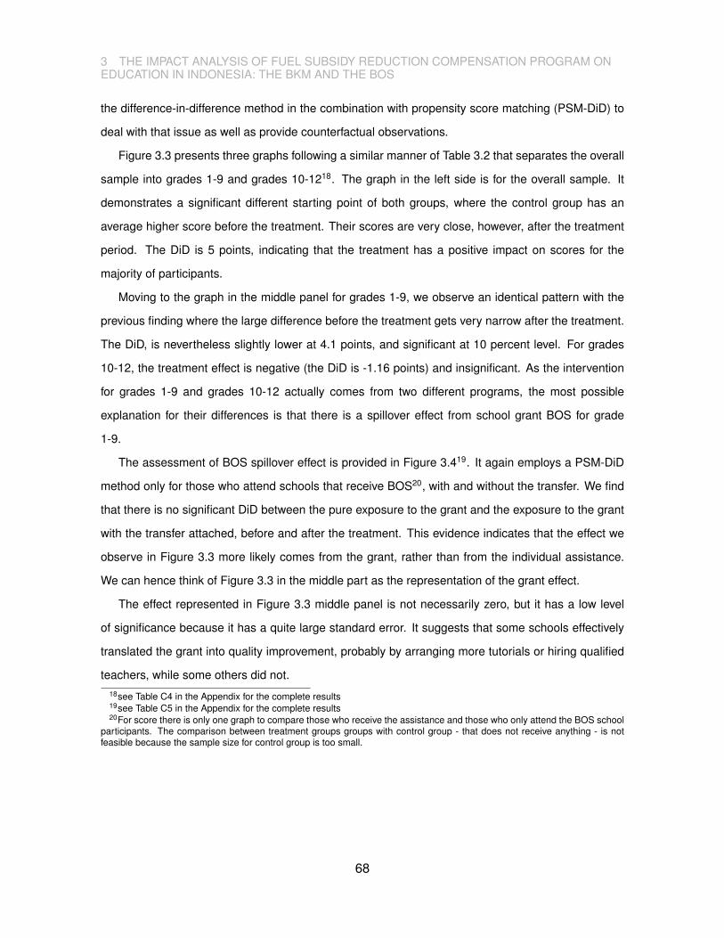
3 THE IMPACT ANALYSIS OF FUEL SUBSIDY REDUCTION COMPENSATION PROGRAM ONEDUCATION IN INDONESIA: THE BKM AND THE BOS
the difference-in-difference method in the combination with propensity score matching (PSM-DiD) to
deal with that issue as well as provide counterfactual observations.
Figure 3.3 presents three graphs following a similar manner of Table 3.2 that separates the overall
sample into grades 1-9 and grades 10-1218. The graph in the left side is for the overall sample. It
demonstrates a significant different starting point of both groups, where the control group has an
average higher score before the treatment. Their scores are very close, however, after the treatment
period. The DiD is 5 points, indicating that the treatment has a positive impact on scores for the
majority of participants.
Moving to the graph in the middle panel for grades 1-9, we observe an identical pattern with the
previous finding where the large difference before the treatment gets very narrow after the treatment.
The DiD, is nevertheless slightly lower at 4.1 points, and significant at 10 percent level. For grades
10-12, the treatment effect is negative (the DiD is -1.16 points) and insignificant. As the intervention
for grades 1-9 and grades 10-12 actually comes from two different programs, the most possible
explanation for their differences is that there is a spillover effect from school grant BOS for grade
1-9.
The assessment of BOS spillover effect is provided in Figure 3.419. It again employs a PSM-DiD
method only for those who attend schools that receive BOS20, with and without the transfer. We find
that there is no significant DiD between the pure exposure to the grant and the exposure to the grant
with the transfer attached, before and after the treatment. This evidence indicates that the effect we
observe in Figure 3.3 more likely comes from the grant, rather than from the individual assistance.
We can hence think of Figure 3.3 in the middle part as the representation of the grant effect.
The effect represented in Figure 3.3 middle panel is not necessarily zero, but it has a low level
of significance because it has a quite large standard error. It suggests that some schools effectively
translated the grant into quality improvement, probably by arranging more tutorials or hiring qualified
teachers, while some others did not.18see Table C4 in the Appendix for the complete results19see Table C5 in the Appendix for the complete results20For score there is only one graph to compare those who receive the assistance and those who only attend the BOS school
participants. The comparison between treatment groups groups with control group - that does not receive anything - is notfeasible because the sample size for control group is too small.
68
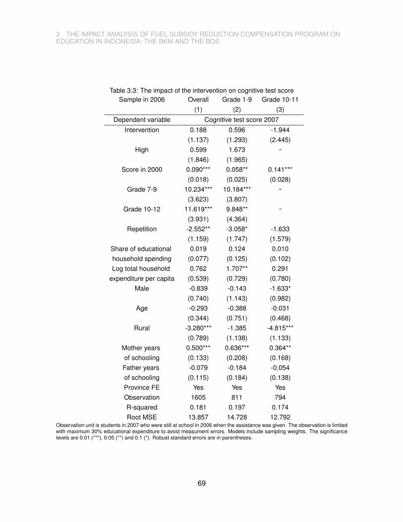
3 THE IMPACT ANALYSIS OF FUEL SUBSIDY REDUCTION COMPENSATION PROGRAM ONEDUCATION IN INDONESIA: THE BKM AND THE BOS
Table 3.3: The impact of the intervention on cognitive test scoreSample in 2006 Overall Grade 1-9 Grade 10-11
(1) (2) (3)
Dependent variable Cognitive test score 2007
Intervention 0.188 0.596 -1.944(1.137) (1.293) (2.445)
High 0.599 1.673 -(1.846) (1.965)
Score in 2000 0.090*** 0.058** 0.141***(0.018) (0.025) (0.028)
Grade 7-9 10.234*** 10.184*** -(3.623) (3.807)
Grade 10-12 11.619*** 9.848** -(3.931) (4.364)
Repetition -2.552** -3.058* -1.633(1.159) (1.747) (1.579)
Share of educational 0.019 0.124 0.010household spending (0.077) (0.125) (0.102)Log total household 0.762 1.707** 0.291
expenditure per capita (0.539) (0.729) (0.780)Male -0.839 -0.143 -1.633*
(0.740) (1.143) (0.982)Age -0.293 -0.388 -0.031
(0.344) (0.751) (0.468)Rural -3.280*** -1.385 -4.815***
(0.789) (1.138) (1.133)Mother years 0.500*** 0.636*** 0.364**of schooling (0.133) (0.208) (0.168)Father years -0.079 -0.184 -0.054of schooling (0.115) (0.184) (0.138)Province FE Yes Yes YesObservation 1605 811 794R-squared 0.181 0.197 0.174Root MSE 13.857 14.728 12.792
Observation unit is students in 2007 who were still at school in 2006 when the assistance was given. The observation is limitedwith maximum 30% educational expenditure to avoid measument errors. Models include sampling weights. The significancelevels are 0.01 (***), 0.05 (**) and 0.1 (*). Robust standard errors are in parentheses.
69

3 THE IMPACT ANALYSIS OF FUEL SUBSIDY REDUCTION COMPENSATION PROGRAM ONEDUCATION IN INDONESIA: THE BKM AND THE BOS
Figure 3.3: PSM-DiD analysis of cognitive test score for overall sample (left), grade 1-9 (middle) andgrade 10-12 (right)
Treatment group: receiving the transfer. Control group: not receiving the transfer.
Figure 3.4: PSM-DiD analysis of cognitive test score to test BOS spillover effect grade1-9
3.4.3 The impact of assistance on educational attainment
Table 3.4 presents the impact of assistance on educational attainment for the overall sample,
grades 1-9 and grades 10-12. The poisson regression is shown with the coefficients that are in-
terpreted as the incidence rate ratio. The result concludes that there is not enough evidence of
intervention having an association with the increase in attainment for neither the overall sample nor for
the subsamples. Instead, the effect of past scholarship programs seems to be more significant after
controlling for the educational level. The expected incidence rate for the increase in attainment with
having exposure to the period of the past scholarship after controlling for educational level is 1.133
times higher or 13.3 percent difference for overall sample. It is slightly higher about 13.5 percent
difference for grades 1-9. In contrast the marginal effect of high is not tractable for grades 10-12 as
all of them are assumed to have gotten exposed to the period of JPS scholarship program.
Among the control variables in overall sample, past attainment, educational level, repetition, log
total household expenditure per capita, gender, age and parental educational attainment are im-
70

3 THE IMPACT ANALYSIS OF FUEL SUBSIDY REDUCTION COMPENSATION PROGRAM ONEDUCATION IN INDONESIA: THE BKM AND THE BOS
portant elements to explain the variation of the increase on attainment. For instance, a student
experiencing at least one repetition has an expected increase on attainment 12.3 percent less than
a student without repetition, holding other factors constant. Additionally, a 10 percent difference in
spending for total household expenditure per capita is associated with a 12 percent difference on the
increase of attainment. Also, male seems to have lower rate of attainment compared to female with
2.8 percent difference. And finally, 10 percent difference of mother education is associated with 4
percent difference on student increase on educational attainment, and in case of father education is
3 percent difference.
The information from grades 1-9 is quite similar to the information from overall sample. Higher
graders, however, face a slightly different situation where repetition and total household expenditure
per capita reduce the significance levels. Meanwhile, parental educational attainment is not significant
at all for schooling improvement. Instead, the increase of 10 percent share of household educational
expenditure and of total household expenditure are associated with 1 percent and 4 percent differ-
ences of attainment consecutively.
71

3 THE IMPACT ANALYSIS OF FUEL SUBSIDY REDUCTION COMPENSATION PROGRAM ONEDUCATION IN INDONESIA: THE BKM AND THE BOS
Table 3.4: The impact of the intervention on educational attainment using Poisson regressionSample in 2006 Overall Grade 1-9 Grade 10-12
(1) (2) (3)
Dependent variable Educational attainment 2007
intervention 0.994 0.995 0.986(0.006) (0.007) (0.009)
High 1.133*** 1.135*** -(0.009) (0.011)
Ed. attainment 2000 0.951*** 0.930*** 1.030***(0.014) (0.006) (0.005)
Grade 7-9 1.147*** 1.100*** -(0.014) (0.015)
Grade 10-12 1.128*** 1.056** -(0.020) (0.023)
Repetition 0.877*** 0.860*** 0.963*(0.007) (0.010) (0.008)
Share of educational 1.000 1.001 1.001*household spending (0.0005) (0.007) (0.0004)Log total household 1.012*** 1.012*** 01.004*
expenditure per capita (0.003) (0.004) (0.002)Male 0.972*** 0.967*** 0.995
(0.005) (0.006) (0.004)Age 1.142*** 1.161*** 1.029***
(0.004) (0.005) (0.004)Rural 0.997 1.002 0.998
(0.005) (0.007) (0.005)Mother years 1.004*** 1.005*** 1.001of schooling (0.001) (0.001) (0.007)Father years 1.003*** 1.005*** 1.000of schooling (0.001) (0.001) (0.001)Province FE Yes Yes YesObservation 4978 4178 800
Log pseudolikelihood -9849.006 -7954.526 -1850.511Observation unit is students in 2007 who were still at school in 2006 when the assistance was given. The observation is limitedwith maximum 30% educational expenditure to avoid measurement errors. Models include sampling weights. The significancelevels are 0.01 (***), 0.05 (**) and 0.1 (*). Robust standard errors are in parentheses.
A second approach is portrayed in Figure 3.5 using PSM-DiD. Contrary to the previous finding, we
detect that the DiD of educational attainment is significant for grade 1-9. After one year of intervention,
the schooling period of 1-9 graders extends for another 4 months on the average. However, this effect
vanishes for grades 10-12, which again evokes the suspicion that the school grant might endorse the
72

3 THE IMPACT ANALYSIS OF FUEL SUBSIDY REDUCTION COMPENSATION PROGRAM ONEDUCATION IN INDONESIA: THE BKM AND THE BOS
Figure 3.5: PSM-DiD analysis of educational attainment for overall sample (left), grade 1-9 (middle)and grade 10-12 (right)
Treatment group: receiving the transfer. Control group: not receiving the transfer.
impact. The assessment of school grant spillover effect for grades 1-9 is presented in the next figure.
Figure 3.6 shows the DiD for two treatment groups - BOS and BOS with individual transfer - and
one control group. We compare BOS without transfer and with transfer on the left side, BOS without
transfer and control in the middle, and BOS with transfer and control on the right side.
Figure 3.6: PSM-DiD analysis of educational attainment to test BOS spillover effect grade 1-9
Treatment groups: (i) attending BOS school and receiving the transfer; (ii) attending BOS school. Control group: attending nonBOS school and receiving no transfer.
As was the case for score, there in no significant DiD between BOS with and without transfer. The
positive effect of intervention, therefore, is most likely rooted from the school grant that expands the
access of education through the offer of lower or even no tuition fees and abolish other administration
fees. As for the comparison with control group, both treatments show no significant DiD either. More-
over, the control group always has a relatively higher educational attainment that fits the description
73

3 THE IMPACT ANALYSIS OF FUEL SUBSIDY REDUCTION COMPENSATION PROGRAM ONEDUCATION IN INDONESIA: THE BKM AND THE BOS
of how rich private schools typically perform. It indicates that the performance of subsidies capacity
did not achieve the same level of what the private spending does on attainment. Yet, it might be
worse without the subsidies. In addition to that, there is a concern that the household adjust their
educational spending back to the level before receiving the transfer. If this is the case, it might explain
why the transfer does not effectively increase the attainment.
3.4.4 The impact of the assistance on household educational expenditure
Table 3.5 presents the instrumental variable models for the overall sample (column 1) and sub-
samples (column 2 for grades 1-9 and column 3 for grades 10-12). Each model consists of the
first and second stage regressions. The F-test of the first stage regressions for the overall sample
suggests that the instruments are jointly not weak. Moreover, the individual t-statistics indicates
that each instrument is relevant in explaining the probability of being selected into the assistance
program. Moving to the second stage regression, the intervention is associated with a decrease
on household educational spending. Households anticipate the transfer by reducing the share of
educational expenditure by 1.23 percent on average, controlling for other factors. This is a clear sign
of crowding out household expenditure. Additionally, experiencing the past scholarship period, having
a higher total household expenditure per capita, being a male, being older and living in rural areas
are also associated with the lower share of household educational spending, while higher grades and
higher parental attainment support more expense.
When examining the subsamples, we observe that results from the overall sample is mostly driven
by grades 1-9 that yield identical significant factors except for repetition, gender and age. However,
the intervention does not have a significant association with educational expenditure for grades 10-12.
74

3 THE IMPACT ANALYSIS OF FUEL SUBSIDY REDUCTION COMPENSATION PROGRAM ONEDUCATION IN INDONESIA: THE BKM AND THE BOS
Table 3.5: The impact of the intervention on household educational expenditureSample in 2006 Overall Grade 1-9 Grade 10-12
(1) (2) (3)1st stage 2nd stage 1st stage 2nd stage 1st stage 2nd stage
Dependent variable Educational attainment 2007Mistargeting 0.485*** - 0.514*** - 0.300*** -
(0.017) (0.018) (0.053)District election 2005 -0.062*** - -0.072*** - 0.018 -
(0.013) (0.015 (0.018)intervention - -1.228*** -0.951*** - -9.605
(0.323) (0.308) (2.762)High -0.026* -0.503* -0.012 -0.529* - -
(0.025) (0.271) (0.024) (0.274)Ed. spending 2000 -0.004* 0.195*** -0.008** 0.256*** -0.005 0.051
(0.002) (0.053) (0.003) (0.045) (0.001) (0.084)Grade 7-9 -0.053** 2.215*** -0.062** 1.756*** - -
(0.024) (0.268) (0.026) (0.270)Grade 10-12 -0.145*** 4.661*** -0.112*** 5.037*** - -
(0.039) (0.439) (0.041) (0.496)Repetition -0.028 0.315* -0.044** 0.178 0.009 0.420
(0.017) (0.190) (0.020) (0.197) (0.028) (0.623)Log total household -0.011* -0.739*** -0.012 -0.565*** -0.004** -1.456***
expenditure per capita (0.007) (0.075) (0.008) (0.077) (0.009) (0.207)Male 0.029** -0.256* 0.028** -0.212 0.004 -0.644
(0.012) (0.134) (0.013) (0.139) (0.018) (0.426)Age -0.007* -0.182*** -0.003 -0.046 0.0001 -0.421**
(0.004) (0.043) (0.005) (0.045) (0.009) (0.180)Rural 0.006 -0.715*** -0.007 -0.800*** -0.021 0.280
(0.013) (0.146) (0.015) (0.152) (0.020) (0.463)Mother years -0.006*** 0.081*** -0.006*** 0.067*** -0.005* 0.161**of schooling (0.002) (0.025) (0.002) (0.026) (0.003) (0.078)Father years 0.003 0.132*** 0.002 0.152*** 0.002 0.040of schooling (0.002) (0.023) (0.002) (0.024) (0.003) (0.074)Province FE Yes Yes Yes Yes Yes YesObservation 4986 4812 804
Endogeneity test [0.014] [0.142] [0.389]F test 431.82 455.81 16.84
Hansen J stat [0.424] [0.286] [0.000]Observation unit is students in 2007 who were still at school in 2006 when the assistance was given. The observation is limitedwith maximum 30% educational expenditure to avoid measurement errors. Models include sampling weights. The significancelevels are 0.01 (***), 0.05 (**) and 0.1 (*). Robust standard errors are in parentheses.
Figure 3.7 provides a PSM-DiD approach. We find that none of the samples show a significant
DiD concerning the treatment effect on household educational expenditure, even though all signs are
negative. The next step is to test BOS spillover effect for grades 1-9 since some spending in education
must have been gone after the school grant was introduced.
Testing the spillover effect reveals that the effect of BOS with and without the transfer on household
expenditure in education (Figure 3.8) is similar. It suggests that the marginal effect of individual
assistance seems to be insignificant on spending. Comparing them to the control group shows
75
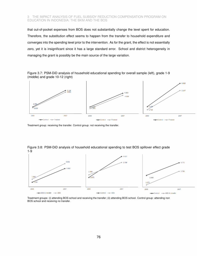
3 THE IMPACT ANALYSIS OF FUEL SUBSIDY REDUCTION COMPENSATION PROGRAM ONEDUCATION IN INDONESIA: THE BKM AND THE BOS
that out-of-pocket expenses from BOS does not substantially change the level spent for education.
Therefore, the substitution effect seems to happen from the transfer to household expenditure and
converges into the spending level prior to the intervention. As for the grant, the effect is not essentially
zero, yet it is insignificant since it has a large standard error. School and district heterogeneity in
managing the grant is possibly be the main source of the large variation.
Figure 3.7: PSM-DiD analysis of household educational spending for overall sample (left), grade 1-9(middle) and grade 10-12 (right)
Treatment group: receiving the transfer. Control group: not receiving the transfer.
Figure 3.8: PSM-DiD analysis of household educational spending to test BOS spillover effect grade1-9
Treatment groups: (i) attending BOS school and receiving the transfer; (ii) attending BOS school. Control group: attending nonBOS school and receiving no transfer.
76

3 THE IMPACT ANALYSIS OF FUEL SUBSIDY REDUCTION COMPENSATION PROGRAM ONEDUCATION IN INDONESIA: THE BKM AND THE BOS
3.4.5 Heterogeneity analysis
Table 3.6: Impact for subgroupsGrade 1-9 Grade 10-12
(1) (2) (3) (1) (2) (3)
Female 3.569 0.154 -0.095 -1.102 -0.115 0.183Male 5.196 0.240** -0.456 -5.584 -0.096 -2.522**Urban 6.413* 0.157 -1.078* -1.344 -0.056 0.931Rural 2.594 0.325*** 0.014 -5.379 -0.157 -1.407
Non Java residence 1.200 0.199 -0.112 -0.123 -0.087 -0.600Java residence 6.425** 0.293*** -0.094 -1.323 -0.149 0.065
Q1 - 0.162 -0.124 - - -Q2 2.553 0.280 -0.784 -6.270 -0.439 0.600Q3 13.624** 0.212 -0.577 - -0.432 0.133Q4 6.601** 0.104 0.084 -1.927 -0.251 1.285
Note: (1) is cognitive test score; (2) is educational attainment; (3) is household expenditure in education. Q1-Q4 are wealthindex quantiles. Blank cells indicates there is not enough observation to analyse in the related subgroups. The method isDiD-PSM. The significance levels are 0.01 (***), 0.05 (**) and 0.1 (*).
Table 3.6 presents the results of PSM-DiD for various socio-economics and demographic groups.
It consists of two different educational levels and assesses the impact on learning as well as spending
outcomes. We find that the participants grade 1-9 who live in urban areas, in Java and are from
the richer households have a positive impact on the increase of cognitive test scores. Futhermore,
being male, living in rural areas and living in Java are beneficial to increasing participants’attainment.
Contrarily, living in urban areas means a decrease on spending, given the subsidy.
We need to keep in mind, however, that the grant is probably the main reason behind the significant
impact of the treatment for the compulsory grades. This suspicion is strengthened by evidence from
higher grades, where the intervention has no impact on education outcomes for different subgroups.
The transfer for senior secondary level, instead, substitutes for household expenditure in education
for males.
3.5 Conclusions and policy implications
Education subsidies are the answer to the question of how governments can provide access
to education through income redistribution schemes. In this paper, we point out several aspects
concerning two education subsidies given in Indonesia as the consequence of increasing domestic
oil prices during 2001 to 2005. The education subsidies of our interest are Bantuan Khusus Murid
(BKM) in the form of direct transfers to households and Bantuan Operational Sekolah (BOS) as the
grant for schools, where schools can send a fraction of it as an out-of-pocket expense to poor students.
77
3 THE IMPACT ANALYSIS OF FUEL SUBSIDY REDUCTION COMPENSATION PROGRAM ONEDUCATION IN INDONESIA: THE BKM AND THE BOS
This variable, therefore, is a combination of a targeted subsidy and a derivation of universal subsidy
that were implemented at the same period of time.
Our data from the Indonesian Family Life Survey 2007 simply unify both transfers into one single
treatment variable and this variable documents the assistance received in the 2006/2007 academic
year. We examine the impact of the intervention on two education outcomes, as well as on household
educational expenditure. Our study contributes to the literature by identifying barriers that hold back
the optimal impact of educational subsidies and the impact size under such constraints.
The procedure defining who is eligible for BKM has a poverty treshold as the baseline determines
the priority provinces/districs and the amount of the transfer. However, schools have the final nomi-
nation list - also for out-of-pocket spending from BOS - and even with very clear guidelines, schools
are able to select the nominees according to their own judgment because there is no strict monitoring
system of the participants profile. Our preliminary analysis indicates mistargeting is an issue for this
particular policy. We find that approximately 10 percent of the funding was mistargeted to non-poor
students and 80 percent of the poor was excluded from the intervention. However, the take up rate
for BKM was not large and the literature suggests that out-of-pocket expense from BOS funding was
also little. Those might be the reasons why we observe quite a large amount of exclusion. Even if
the targeting had been perfectly correct, the exclusion rate would only be reduced to 70 percent. This
indicates that the coverage of the subsidies was too small.
We do not find a significant association between the intervention and education outcomes in the
cross section analysis. The DiD-PSM approach shows, however, that cognitive test scores increase
by 5 points for the overall sample and educational attainment increases around 4 months for grades
1-9 after one year of intervention. In the latter case, further examination suggests that the positive
effects are most likely coming from the BOS instead of the individual subsidies. The grant size
for each student was considerably large and implemented without an adequate monitoring system.
Nevertheless, this program was still able to deliver some positive outcomes in the short run. This
example shows that universal subsidies can work well and would possibly be better with more effective
management. Moreover, there seems to be a long term effect of the past subsidies on educational
attainment. Controlling for education level, exposure to the JPS scholarship period is associated with
13 percent difference in educational attainment.
Educational spending has a different story. Intervention is associated with a 1 percent decrease
in household expenditure on education. In addition, we find that the transfer has a substitution effect
78
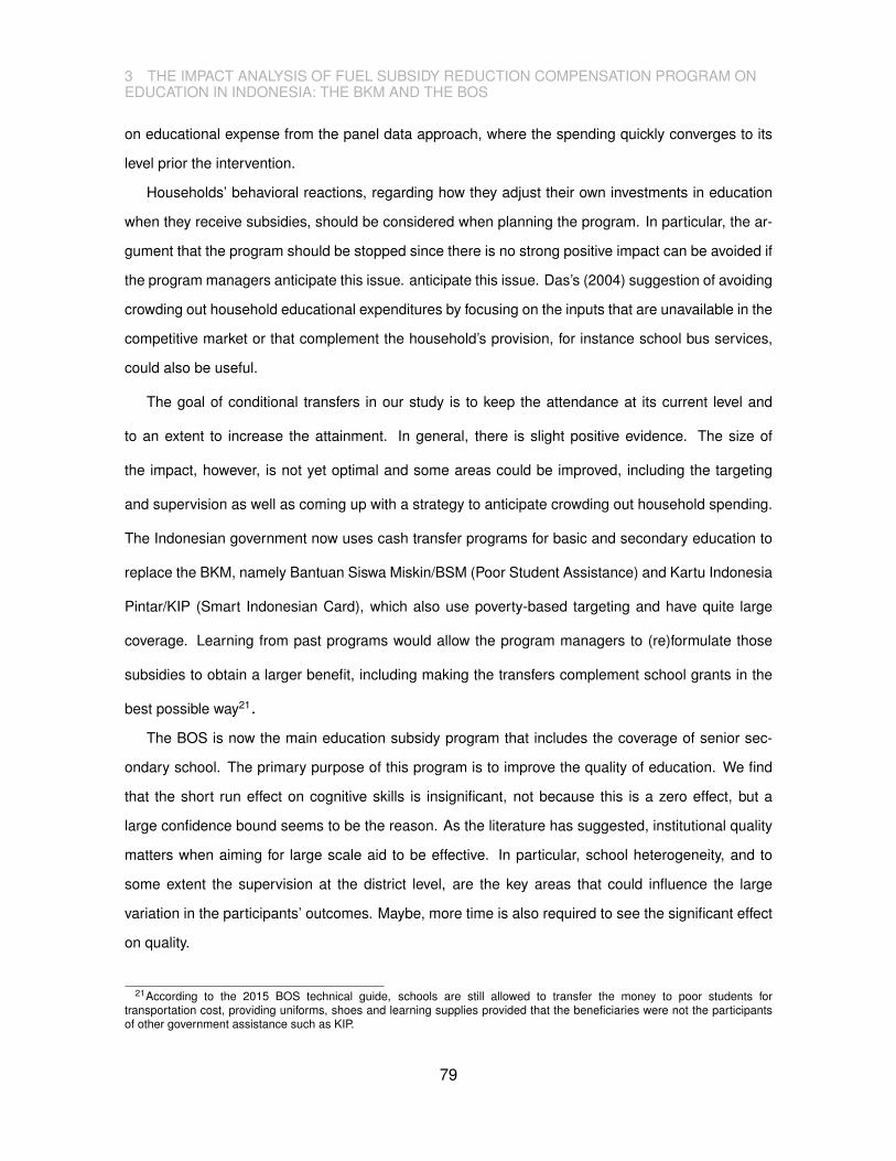
3 THE IMPACT ANALYSIS OF FUEL SUBSIDY REDUCTION COMPENSATION PROGRAM ONEDUCATION IN INDONESIA: THE BKM AND THE BOS
on educational expense from the panel data approach, where the spending quickly converges to its
level prior the intervention.
Households’ behavioral reactions, regarding how they adjust their own investments in education
when they receive subsidies, should be considered when planning the program. In particular, the ar-
gument that the program should be stopped since there is no strong positive impact can be avoided if
the program managers anticipate this issue. anticipate this issue. Das’s (2004) suggestion of avoiding
crowding out household educational expenditures by focusing on the inputs that are unavailable in the
competitive market or that complement the household’s provision, for instance school bus services,
could also be useful.
The goal of conditional transfers in our study is to keep the attendance at its current level and
to an extent to increase the attainment. In general, there is slight positive evidence. The size of
the impact, however, is not yet optimal and some areas could be improved, including the targeting
and supervision as well as coming up with a strategy to anticipate crowding out household spending.
The Indonesian government now uses cash transfer programs for basic and secondary education to
replace the BKM, namely Bantuan Siswa Miskin/BSM (Poor Student Assistance) and Kartu Indonesia
Pintar/KIP (Smart Indonesian Card), which also use poverty-based targeting and have quite large
coverage. Learning from past programs would allow the program managers to (re)formulate those
subsidies to obtain a larger benefit, including making the transfers complement school grants in the
best possible way21.
The BOS is now the main education subsidy program that includes the coverage of senior sec-
ondary school. The primary purpose of this program is to improve the quality of education. We find
that the short run effect on cognitive skills is insignificant, not because this is a zero effect, but a
large confidence bound seems to be the reason. As the literature has suggested, institutional quality
matters when aiming for large scale aid to be effective. In particular, school heterogeneity, and to
some extent the supervision at the district level, are the key areas that could influence the large
variation in the participants’ outcomes. Maybe, more time is also required to see the significant effect
on quality.
21According to the 2015 BOS technical guide, schools are still allowed to transfer the money to poor students fortransportation cost, providing uniforms, shoes and learning supplies provided that the beneficiaries were not the participantsof other government assistance such as KIP.
79

Appendix A
Table A1: Freedom House and Maddison GDP per capitaDependent variable: 5 year 10 year 20 year 5 year average
democracy (M1) (M2) (M3) (M4)Mean equation (µ)
Lag democracy 1.094*** -0.714** -1.638*** 1.991***(1.673) (0.261) (0.190) (0.168)
Lag log income per capita -0.197 -0.305 0.326* -0.223(0.140) (0.271) (0.169) (0.137)
OECD (D) 2.529* 0.997 -0.432 3.696***(1.319) (0.954) (0.661) (1.293)
Country fe Yes Yes Yes YesYear fe Yes Yes Yes Yes
Scale equation (σ)Lag Democracy -*** + No -
Lag Log income per capita +*** +*** +*** +**OECD (D) +** +*** - +Country fe No No No No
Year fe No No No YesZero inflation equation (ν)
Lag democracy -2.342*** 1.357 458.996 -10.100***(0.643) (1.335) (8.142e+4) (1.206)
Lag log income per capita -0.074 -1.219** -10.590 -0.022(0.313) (0.543) (1.052e+4) (0.075)
OECD (D) -20.843 -18.525 -432.161 -10.100(4.515e+4) (5.565e+6) (4.841e+7) (1.206)
Country fe Yes Yes Yes NoYear fe Yes No Yes Yes
One inflation equation (τ )Lag democracy 9.722*** 4.274** -16.046*** 21.497***
(2.486) (2.119) (5.124) (6.572)Lag log income per capita 5.056** 1.985 20.303*** 4.914
(2.221) (2.253) (4.523) (3.481)OECD (D) -12.680 19.482 -52.419 -23.898
(1.707e+4) (3.975e+4) (5.307e+1) (6.996e+3)Country fe Yes Yes Yes Yes
Year fe Yes Yes Yes YesObservation 858 384 141 858
Country 136 127 88 136Global deviance -148.574 -146.031 -256.316 -402.312
AIC 727.426 659.969 309.684 215.688SBC 2809.942 2252.078 1144.183 1684.861
The coefficients are in logit form for the equations for µ and σ, in log form for the equations for ν and τ . The equation for σ only shows thedirection of relationship and its significance level. Significance levels are 0.1 (*), 0.05 (**) and 0.01 (***). Standard errors are in parentheseswith “qr” type, which assumes there is no correlation among the parameters. Models M1-M3 are estimated using 5, 10 and 20 year intervals,respectively. Country fixed-effects and year fixed-effects are used only when the algorithms converge.
80
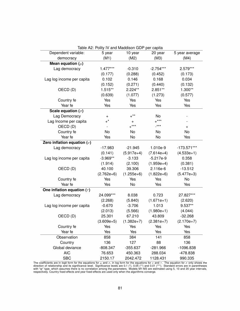
Table A2: Polity IV and Maddison GDP per capitaDependent variable: 5 year 10 year 20 year 5 year average
democracy (M1) (M2) (M3) (M4)Mean equation (µ)
Lag democracy 1.477*** -0.310 -2.754*** 2.579***(0.177) (0.288) (0.452) (0.173)
Lag log income per capita 0.102 0.146 0.168 0.034(0.152) (0.271) (0.440) (0.132)
OECD (D) 1.515** 2.224** 2.851** 1.300**(0.639) (1.077) (1.273) (0.577)
Country fe Yes Yes Yes YesYear fe Yes Yes Yes Yes
Scale equation (σ)Lag Democracy + +** No -
Lag Income per capita +* + +*** -OECD (D) - +*** -*** +Country fe No No No No
Year fe Yes No No YesZero inflation equation (ν)
Lag democracy -17.983 -21.945 1.010e-9 -173.571***(0.141) (5.917e+4) (7.614e+4) (4.533e+1)
Lag log income per capita -3.969** -3.133 -5.217e-9 0.358(1.914) (2.100) (1.959e+4) (0.381)
OECD (D) 40.100 39.306 2.116e-6 -13.512(2.762e+6) (1.255e+6) (1.822e+6) (5.477e+3)
Country fe Yes Yes Yes NoYear fe Yes No Yes Yes
One inflation equation (τ )Lag democracy 24.099*** 8.038 0.723 27.827***
(2.268) (5.840) (1.671e+1) (2.620)Lag log income per capita -0.670 -3.706 1.013 9.537**
(2.013) (5.566) (1.980e+1) (4.044)OECD (D) 25.301 67.210 43.809 -32.268
(3.609e+5) (1.382e+7) (2.381e+7) (2.170e+7)Country fe Yes Yes Yes Yes
Year fe Yes Yes Yes YesObservation 858 384 141 858
Country 136 127 88 136Global deviance -808.347 -355.637 -281.966 -1096.838
AIC 76.653 450.363 288.034 -478.838SBC 2150.17 2042.472 1128.431 990.335
The coefficients are in logit form for the equations for µ and σ, in log form for the equations for ν and τ . The equation for σ only shows thedirection of relationship and its significance level. Significance levels are 0.1 (*), 0.05 (**) and 0.01 (***). Standard errors are in parentheseswith “qr” type, which assumes there is no correlation among the parameters. Models M1-M3 are estimated using 5, 10 and 20 year intervals,respectively. Country fixed-effects and year fixed-effects are used only when the algorithms converge.
81

Table A3: Results with annual data for income variable Penn World Table GDPDependent var. Freedom House Polity IV
Equation µ σ ν τ µ σ ν τDemocracy
lag 1 3.674*** -*** -20.434*** 30.028*** 4.510*** -*** -1.516e+4 151.446***(0.104) (1.509) (3.177) (0.066) (1.116e+5) (36.567)
lag 2 -0.163 +** 0.361 2.480 0.064 - 100.58 3.596(0.132) (1.354) (3.475) (0.061) (1.810e+3) (48.161)
lag 3 0.078 +*** 0.159 0.154 -0.061 +*** 609.54 8.173(0.125) (1.166) (3.009) (0.075) (1.803e+3) (43.408)
lag 4 -0.002 -*** -1.414 0.364 0.103 -* -257.12** 16.027(0.117) (1.088) (3.095) (0.085) (107.55) (27.584)
lag 5 -0.014 + 0.799 0.480 -0.151** +*** 520.15*** -4.244**(0.098) (0.799) (2.280) (0.072) (151.72) (2.071)
Log income per capitalag 1 0.001 +** -0.850 -3.372 -0.055 -*** 142.06*** 4.585
(0.209) (1.300) (0.507) (0.119) (29.54) (8.757)lag 2 -0.075 -*** 1.009 5.199 -0.299* -*** -18.280 1.503
(0.300) (1.931) (7.097) (0.165) (26.890) (11.994)lag 3 -0.021 +*** -0.399 4.717 0.204 +*** -79.120*** -8.169
(0.274) (1.938) (5.960) (0.141) (26.650) (11.713)lag 4 0.035 -*** -0.450 -11.012*** 0.372*** +*** 32.200 1.254
(0.270) (1.833) (5.168) (0.124) (31.630) (11.432)lag 5 -0.067 + 0.490 6.326** -0.191* -*** -34.050 2.387
(0.191) (1.146) (2.810) (0.105) (24.660) (6.585)OECD (D) 0.367*** - -1.007 -0.314 0.389* + 1081.44 -0.047
(0.135) (0.798) (0.507) (0.220) (112.040) (1.120)Country fe Yes No No No Yes No No No
Year fe Yes No No No Yes No No NoObservation 2427 2427
Country 117 117Global deviance -2391.466 -4665.036
AIC -2011.466 -4283.036SBC -910.528 -3176.034
µ is the mean equation, σ is the scale equation; ν is the zero inflation equation; τ is the one inflation equation. The coefficients are in logitform for the equations for µ and σ, in log form for the equations for ν and τ . The equation for σ only shows the direction of relationship and itssignificance level. Significance levels are 0.1 (*), 0.05 (**) and 0.01 (***). Standard errors are in parentheses with “qr” type, which assumes thereis no correlation among the parameters. Country fixed-effects and year fixed-effects are used only when the algorithms converge.
82

Table A4: Results with annual data for income variable Maddison GDPDependent var. Freedom House Polity IV
Equation µ σ ν τ µ σ ν τdemocracy
lag 1 4.055*** -*** -23.089*** 31.581*** 4.871*** -*** -156.114*** 145.158***(0.083) (1.389) (3.282) (0.053) (21.681) (29.859)
lag 2 -0.111 - 0.143 2.450 -0.050 +* 0.327 16.385(0.098) (1.322) (3.583) (0.054) (14.229) (37.717)
lag 3 0.126 +*** -0.208 0.714 -0.016 +*** 1.317 3.226(0.087) (1.143) (3.416) (0.081) (13.429) (40.684)
lag 4 -0.154* -*** -1.059 -0.167 0.152 -*** -0.910 20.734(0.085) (1.089) (3.250) (0.087) (12.694) (31.665)
lag 5 -0.021 + 0.272 1.808 -0.295*** +*** 0.671 -5.165***(0.071) (0.805) (2.191) (0.061) (7.005) (1.905)
Log income per capitalag 1 0.241 -*** -0.152 -6.454 -0.171** -*** 4.595 2.875
(0.174) (1.389) (4.627) (0.086) (4.569) (12.200)lag 2 -0.519** -* -1.293 10.167 -0.086 +** -5.236 -18.968
(0.263) (2.251) (7.762) (0.153) (5.737) (17.490)lag 3 0.274 +*** 0.729 -0.836 0.088 +** 2.525 17.982
(0.225) (1.955) (6.228) (0.151) (5.732) (13.412)lag 4 -0.052 -*** 1.242 -9.003* 0.098 +*** -3.371 -8.728
(0.172) (1.580) (4.719) (0.158) (4.810) (8.741)lag 5 -0.009 +*** -0.507 6.131** -0.032 + 1.621 6.334
(0.117) (0.871) (2.418) (0.108) (2.239) (4.235)OECD (D) -0.250 - -1.629** 1.429*** 0.326** +* -13.210 2.543**
(0.609) (0.781) (0.414) (0.164) (6.644e+4) (1.103)Country fe Yes No No No Yes No No No
Year fe Yes Yes No No Yes Yes No NoObservation 2835 2835
Country 134 134Global deviance -3086.879 -6284.997
AIC -2622.879 -5820.997SBC -1242.526 -4440.624
µ is the mean equation, σ is the scale equation; ν is the zero inflation equation; τ is the one inflation equation. The coefficients are in logitform for the equations for µ and σ, in log form for the equations for ν and τ . The equation for σ only shows the direction of relationship and itssignificance level. Significance levels are 0.1 (*), 0.05 (**) and 0.01 (***). Standard errors are in parentheses with “qr” type, which assumes thereis no correlation among the parameters. Country fixed-effects and year fixed-effects are used only when the algorithms converge.
83

Table A5: Modeling OECD membership as the causal factor of higher democracyDependent variable: 5 year 10 year 5 year average
democracy (M1) (M2) (M3) (M4) (M5) (M6)Mean equation (µ)
Lag democracy 1.290* 0.768 -7.689*** -1.083 1.774** 2.897***(0.706) (0.512) (0.648) (1.035) (0.668) (0.456)
Lag log income per capita 1.137**(0.571)
0.156(0.550)
3.125***(0.408)
0.015(0.698)
0.448(0.619)
-0.103(0.540)
Lag OECD (D) No No No No -0.056 0.420- - - - (0.326) (0.265)
Country fe Yes Yes Yes Yes Yes YesYear fe Yes Yes Yes Yes Yes Yes
Scale equation (σ)Lag democracy -*** + -*** -*** -*** -***
Lag log income per capita No No No No +*** -***Country fe No No No No No No
Year fe No No No No Yes YesZero inflation equation (ν)
Lag democracy 39.259 1.910e-8 6.878e-7 9.840e-7 5.026e-7 -2.045e-9(2.721e+5) (2.514e+5) (1.012e+6) (3.198e+5) (3.503e+5) (7.643e+5)
Lag log income per capita -1.882(3.647e+5)
-5.198e-9(2.531e+5)
6.902e-7(1.429e+6)
6.094e-7(4.101e+5)
-5.185e-7(3.030e+5)
-9.614e-9(7.118e+5)
Lag OECD (D) -27.162 1.920e-8 3.602e-7 1.434e-7 3.774e-7 -1.340e-8(1.622e+5) (2.574e+5) (1.002e+6) (3.166e+5) (2.085e+5) (6.296e+5)
Country fe Yes Yes Yes Yes Yes YesYear fe Yes Yes Yes Yes Yes Yes
One inflation equation (τ )Lag democracy 42.912** 17.176*** 28.873** 5.304** 13.549 19.863**
(1.779e+1) (4.624) (12.680) (2.654) (11.111) (5.168)Lag log income per capita 0.416
(4.265)9.920*(5.802)
5.072***(1.874)
3.499***(3.099)
-11.792(2.708)
1.980(1.668)
Lag OECD (D) 1.434 6.350* 2.336 -0.662 1.409 -5.263(2.822) (3.819) (1.492) (0.968) (4.566) (5.168)
Country fe Yes Yes No No Yes YesYear fe Yes Yes Yes Yes Yes Yes
Observation 216 216 109 109 209 209Country 28 28 28 28 27 27
Global deviance -73.868 -90.084 -47.468 6.457 -102.798 -147.615AIC 166.132 149.916 106.532 160.457 135.202 90.385SBC 571.165 554.950 313.766 367.691 532.939 488.123
The coefficients are in logit form for the equations for µ and σ, in log form for the equations for ν and τ . The equation for σ only shows thedirection of relationship and its significance level. Significance levels are 0.1 (*), 0.05 (**) and 0.01 (***). Standard errors are in parentheseswith “qr” type, which assumes there is no correlation among the parameters. Country fixed-effects and year fixed-effects are used only whenthe algorithms converge. Models with odds number use Freedom House variable, models with even numbers use Polity4 variable. The incomevariable for all models is from Penn World Table.
84
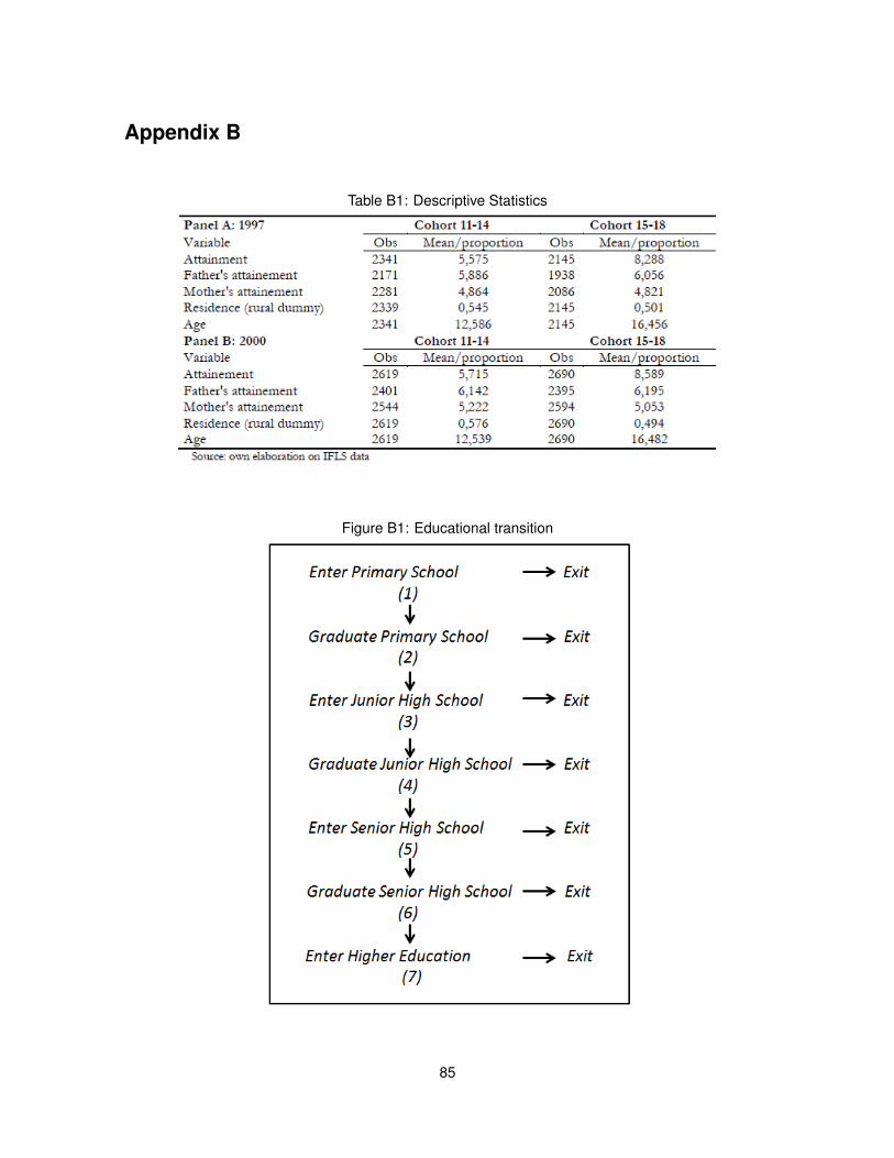
Appendix B
Table B1: Descriptive Statistics
Figure B1: Educational transition
85
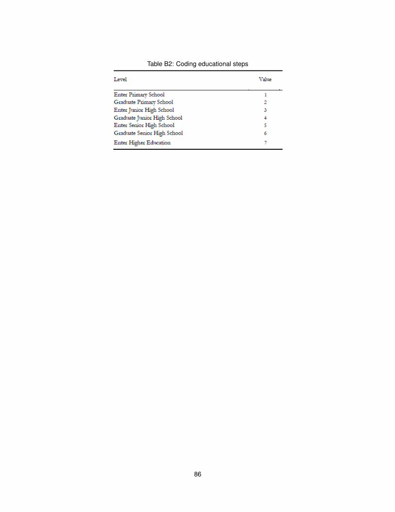
Table B2: Coding educational steps
86

Appendix C
Table C1: The question in IFLS 2007 section DL and DLA (education)DL43, DLA43J & DLA103, DLA103J. From what source was this assistance, and what was the total value?(CIRCLE ALL THAT APPLY)A. GNOTAC. Government (other than BOS)D. Community groupE. Religious groupF. FamilyI. School committeeJ. BOS (DL43) — BOS/BKM Fund (DLA103)K. Foreign government/foundation/individualL. Domestic Non-Government InstitutionSource: IFLS 2007
Table C2: What to spend? BOS Operational Guidelines 2005 & Guide Book 2006No Operational Guidelines 2005 No. Guide Book 20061. Registration form 1. Everything related to registration fees2. Text books and supplementary books for libraries 2. Text books and references books for libraries’ collection3. Teacher trainings for quality improvement 3. School supplies (i.e. writing books, chalks, pencils,
(i.e. MGMP/MKS etc.) practical materials, student registration books, inventorybooks, newspaper subscription, sugar, coffe and tea)
4. School exams and tests 4. Student activities (i.e. remedials, enrichment, sports,arts, scientific activities, scouts, red cross andsimilar activities)
5. School supplies (i.e. notebooks, chalks, pencils 5. School exams, tests, and progress reportsand practical materials)
6. Simple maintenance cost 6. Teaching profession development (i.e. KKG/MGMPand KKKS/MKKS)
7. Monthly bills and service-related cost 7. School maintenancs (i.e. (re)painting,(i.e. electricity and telephone) repair leaking roofs, repair doors and windows,
repair furnitures and others)8. Honorariums for non-permanent teachers and 8. Monthly bills (i.e. electricity, water, telepohone
non-permanent non-teacher personnels including costs for new installment if the vincinityhas covered the network)
9. Student activities (i.e. remedial, enrichment and 9. Honorariums for teachers and educational personnelsextracurricular) who are not paid by central or local government.
Civil service teachers have their welfare incentives asthe responsibility of local government.
10. Transportation cost assistance for students from 10. Transportation costs assistance for students frompoor families poor families
11. Dormitory costs and religious-related equipments 11. Dormitory costs and religious-related equipments forfor religious-based schools religious-based schools
12. BOS management and administration13. The leftover - when available - can be used to spend
for visual aids equipment, instructional medias andschool furnitures
Source: SMERU Newsletter (2006)
87
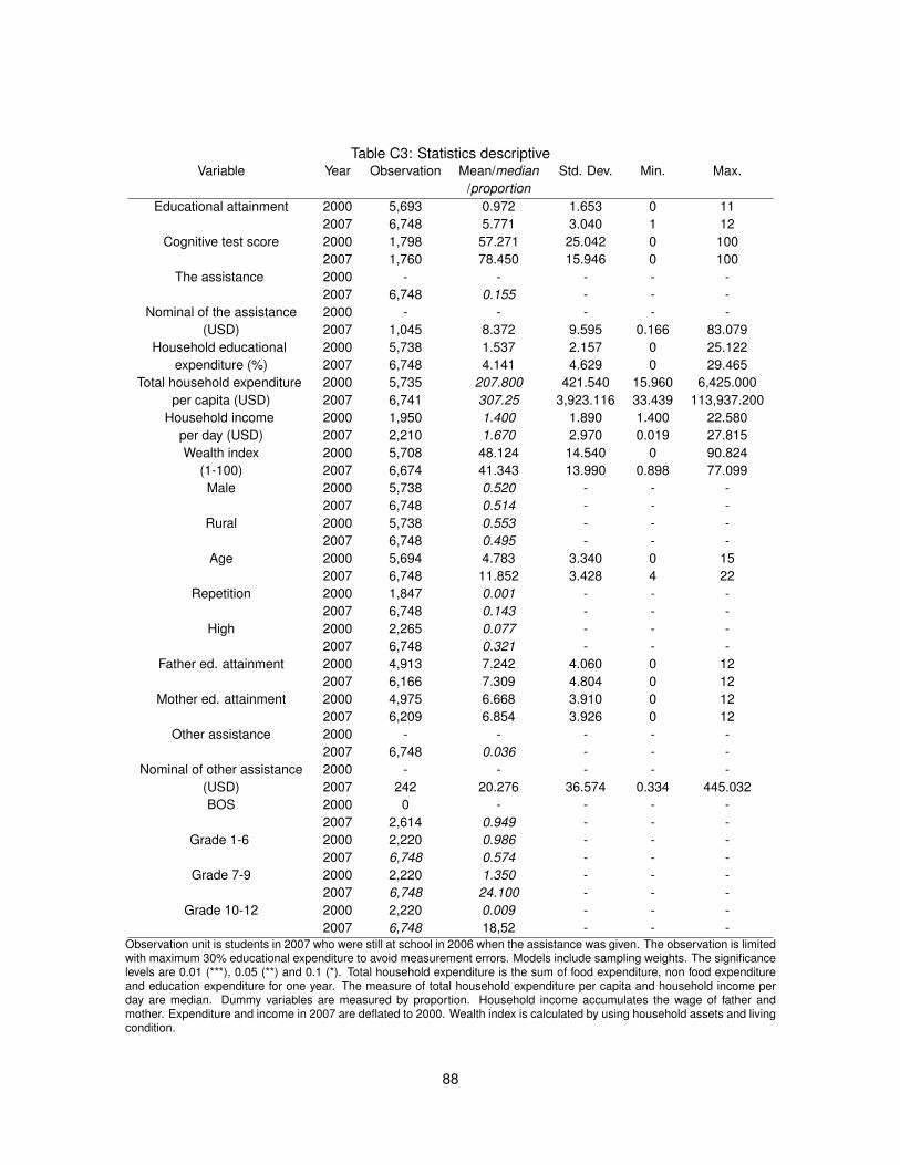
Table C3: Statistics descriptiveVariable Year Observation Mean/median Std. Dev. Min. Max.
/proportionEducational attainment 2000 5,693 0.972 1.653 0 11
2007 6,748 5.771 3.040 1 12Cognitive test score 2000 1,798 57.271 25.042 0 100
2007 1,760 78.450 15.946 0 100The assistance 2000 - - - - -
2007 6,748 0.155 - - -Nominal of the assistance 2000 - - - - -
(USD) 2007 1,045 8.372 9.595 0.166 83.079Household educational 2000 5,738 1.537 2.157 0 25.122
expenditure (%) 2007 6,748 4.141 4.629 0 29.465Total household expenditure 2000 5,735 207.800 421.540 15.960 6,425.000
per capita (USD) 2007 6,741 307.25 3,923.116 33.439 113,937.200Household income 2000 1,950 1.400 1.890 1.400 22.580
per day (USD) 2007 2,210 1.670 2.970 0.019 27.815Wealth index 2000 5,708 48.124 14.540 0 90.824
(1-100) 2007 6,674 41.343 13.990 0.898 77.099Male 2000 5,738 0.520 - - -
2007 6,748 0.514 - - -Rural 2000 5,738 0.553 - - -
2007 6,748 0.495 - - -Age 2000 5,694 4.783 3.340 0 15
2007 6,748 11.852 3.428 4 22Repetition 2000 1,847 0.001 - - -
2007 6,748 0.143 - - -High 2000 2,265 0.077 - - -
2007 6,748 0.321 - - -Father ed. attainment 2000 4,913 7.242 4.060 0 12
2007 6,166 7.309 4.804 0 12Mother ed. attainment 2000 4,975 6.668 3.910 0 12
2007 6,209 6.854 3.926 0 12Other assistance 2000 - - - - -
2007 6,748 0.036 - - -Nominal of other assistance 2000 - - - - -
(USD) 2007 242 20.276 36.574 0.334 445.032BOS 2000 0 - - - -
2007 2,614 0.949 - - -Grade 1-6 2000 2,220 0.986 - - -
2007 6,748 0.574 - - -Grade 7-9 2000 2,220 1.350 - - -
2007 6,748 24.100 - - -Grade 10-12 2000 2,220 0.009 - - -
2007 6,748 18,52 - - -Observation unit is students in 2007 who were still at school in 2006 when the assistance was given. The observation is limitedwith maximum 30% educational expenditure to avoid measurement errors. Models include sampling weights. The significancelevels are 0.01 (***), 0.05 (**) and 0.1 (*). Total household expenditure is the sum of food expenditure, non food expenditureand education expenditure for one year. The measure of total household expenditure per capita and household income perday are median. Dummy variables are measured by proportion. Household income accumulates the wage of father andmother. Expenditure and income in 2007 are deflated to 2000. Wealth index is calculated by using household assets and livingcondition.
88
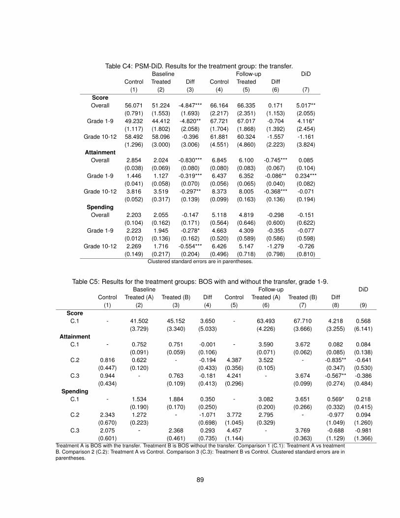
Table C4: PSM-DiD. Results for the treatment group: the transfer.Baseline Follow-up DiD
Control Treated Diff Control Treated Diff(1) (2) (3) (4) (5) (6) (7)
ScoreOverall 56.071 51.224 -4.847*** 66.164 66.335 0.171 5.017**
(0.791) (1.553) (1.693) (2.217) (2.351) (1.153) (2.055)Grade 1-9 49.232 44.412 -4.820** 67.721 67.017 -0.704 4.116*
(1.117) (1.802) (2.058) (1.704) (1.868) (1.392) (2.454)Grade 10-12 58.492 58.096 -0.396 61.881 60.324 -1.557 -1.161
(1.296) (3.000) (3.006) (4.551) (4.860) (2.223) (3.824)Attainment
Overall 2.854 2.024 -0.830*** 6.845 6.100 -0.745*** 0.085(0.038) (0.069) (0.080) (0.080) (0.083) (0.067) (0.104)
Grade 1-9 1.446 1.127 -0.319*** 6.437 6.352 -0.086** 0.234***(0.041) (0.058) (0.070) (0.056) (0.065) (0.040) (0.082)
Grade 10-12 3.816 3.519 -0.297** 8.373 8.005 -0.368*** -0.071(0.052) (0.317) (0.139) (0.099) (0.163) (0.136) (0.194)
SpendingOverall 2.203 2.055 -0.147 5.118 4.819 -0.298 -0.151
(0.104) (0.162) (0.171) (0.564) (0.646) (0.600) (0.622)Grade 1-9 2.223 1.945 -0.278* 4.663 4.309 -0.355 -0.077
(0.012) (0.136) (0.162) (0.520) (0.589) (0.586) (0.598)Grade 10-12 2.269 1.716 -0.554*** 6.426 5.147 -1.279 -0.726
(0.149) (0.217) (0.204) (0.496) (0.718) (0.798) (0.810)Clustered standard errors are in parentheses.
Table C5: Results for the treatment groups: BOS with and without the transfer, grade 1-9.Baseline Follow-up DiD
Control Treated (A) Treated (B) Diff Control Treated (A) Treated (B) Diff(1) (2) (3) (4) (5) (6) (7) (8) (9)
ScoreC.1 - 41.502 45.152 3.650 - 63.493 67.710 4.218 0.568
(3.729) (3.340) (5.033) (4.226) (3.666) (3.255) (6.141)Attainment
C.1 - 0.752 0.751 -0.001 - 3.590 3.672 0.082 0.084(0.091) (0.059) (0.106) (0.071) (0.062) (0.085) (0.138)
C.2 0.816 0.622 - -0.194 4.387 3.522 - -0.835** -0.641(0.447) (0.120) (0.433) (0.356) (0.105) (0.347) (0.530)
C.3 0.944 - 0.763 -0.181 4.241 - 3.674 -0.567** -0.386(0.434) (0.109) (0.413) (0.296) (0.099) (0.274) (0.484)
SpendingC.1 - 1.534 1.884 0.350 - 3.082 3.651 0.569* 0.218
(0.190) (0.170) (0.250) (0.200) (0.266) (0.332) (0.415)C.2 2.343 1.272 - -1.071 3.772 2.795 - -0.977 0.094
(0.670) (0.223) (0.698) (1.045) (0.329) (1.049) (1.260)C.3 2.075 - 2.368 0.293 4.457 - 3.769 -0.688 -0.981
(0.601) (0.461) (0.735) (1.144) (0.363) (1.129) (1.366)Treatment A is BOS with the transfer. Treatment B is BOS without the transfer. Comparison 1 (C.1): Treatment A vs treatmentB. Comparison 2 (C.2): Treatment A vs Control. Comparison 3 (C.3): Treatment B vs Control. Clustered standard errors are inparentheses.
89

Bibliography
Aaberge, R., Mogstad, M., and Peragine, V. (2011). Measuring long-term inequality of opportunity.Journal of Public Economics, 3-4(95): 193–204.
Acemoglu, D., Johnson, S., and Robinson, J. (2001). The Colonial Origins of ComparativeDevelopment: An Empirical Investigation. American Economic Review, 91(5): 1369–1401.
Acemoglu, D., Johnson, S., Robinson, J. A., and Yared, P. (2008). Income and Democracy. AmericanEconomic Review, 98(3): 808–842.
Acemoglu, D., Naidu, S., Restrepo, P., and Robinson, J. A. (2014). Democracy Does Cause Growth.NBER Working Paper Series, (20004).
Al-Samarrai, S., Fasih, T., Hasan, A., and Syukriyah, D. (2014). Assessing the role of the schooloperational grant program (BOS) in improving education outcomes in Indonesia. World Bank GroupJakarta Working Paper, (4133).
Allison, P. D. (2009). Fixed effects regression models. New York: AGE Publications.
Andreoli, F., Havnes, T., and Lefranc, A. (2014). Equalization of opportunity: definitions,implementable conditions and application to early-childhood policy evaluation. In 33rd IARIWConference. Rotterdam, The Netherlands.
Aristotle (1932). Politics. Cambridge, MA: Harvard University Press. Translated by H. Rackham.
Asadullah, M. N., and Yalonetzky, G. (2012). Inequality of educational opportunity in India: Changesover time and across states. World Development, 40(6): 1151–1163.
Asim, S., Chase, R. S., Dar, A., and Schmillen, A. (2015). Improving Education Outcomes in SouthAsia: Findings from a Decade of Impact Evaluations. Policy Research Working Paper World BankGroup Washington DC, (7362).
Bardhan, P. (1999). Democracy and Development: A Complex Relationship. In I. Saphiro, andC. Hacker-Corden (Eds.), Democracy’s Values. Cambridge University Press, 1 edition.
Barro, R. J. (1999). Determinants of Democracy. Journal of Political Economy, 107(S6).
Becker, G. (1993). Human capital: a theoretical and empirical analysis, with special reference toeducation. The University of Chicago Press, 3rd edition.
Behrman, J. R., Gaviria, A., and Székely, M. (2001). Intergenerational Mobility in Latin America.Economia, 2(1): 1–31.
Bhalotra, S., Harttgen, K., and Klasen, S. (2014). The impact of school fees on educational attainmentand the intergenerational transmission of education, Teaching and learning: Achieving quality forall, EFA Global Monitoring Report 2013/14. Discussion paper.
Björklund, A., Jäntti, M., and Roemer, J. (2012). Equality of Opportunity and the distribution of Long-Run Income in Sweden. Social Choice and Welfare, 39(2-3): 675–695.
Bolt, J., and van Zanden, J. L. (2013). The First Update of the Maddison Project: Re-EstimatingGrowth Before 1820. Maddison-Project Working Paper WP-4.
Bourguignon, F., Ferreira, F., and Walton, M. (2007). Equity, efficiency and inequality traps: a researchagenda. Journal of Economic Inequality, 5(2): 235–256.
Buis, M. L. (2007). SEQLOGIT: Stata module to fit a sequential logit model, Statistical SoftwareComponents S456843, Boston College Department of Economics. Revised 25 Oct 2013.
90
Burnside, C., and Dollar, D. (2000). Aid, Policies, and Growth. American Economic Review, 90(4):847–868.
Cameron, L. (2009). Can a public scholarship program successfully reduce school drop-outs in a timeof economic crisis? Evidence from Indonesia. Economics of Education Review, 28(3): 308–317.
Carothers, T., and de Gramont, D. (2011). Aiding Governance in Developing Countries: ProgressAmid Uncertainties. URL http://carnegieendowment.org/files/aiding_governance.pdf.
Cervellati, M., Jung, F., Sunde, U., and Vischer, T. (2014). Income and Democracy: Comment.American Economic Review, 104(2): 707–719.
Checchi, D., and Peragine, V. (2010). Inequality of opportunity in Italy. Journal of Economic Inequality,8(4): 429–450.
Coleman, J., Campbell, E., Hobson, C., and Macpartland, Y. (1966). Equality of educationalopportunity. Discussion paper, US Government Printing Office, Washington DC.
Conn, K. M. (2014). Identifying effective education inteventions in Sub-Saharan Africa: A meta-analysis of rigorous impact evaluations. Ph.D. thesis, Columbia University. URL http://dx.doi.
org/10.7916/D898854G.
Dahan, M., and Gaviria, A. (2001). Sibling correlations and social mobility in Latin America. EconomicDevelopment and Cultural Chan, 49(3): 537–554.
Dahl, R. A. (1971). Polyarchy: Participation and Opposition. Yale University Press.
Dardanoni, V., Fields, G., and Puerta, J. R. R. S. (2005). How demanding should equality ofopportunity be, and how much have we achieved? In S. L. Morgan, D. Grusky, and G. Fields (Eds.),Mobility and Inequality: Frontiers of research in Sociology and Economics. Stanford: StanfordUniversity Press.
Das, J. (2004). Equity in educational expenditures: can government subsidies help? The World BankPolicy Research Working Paper Series, (3249).
Das, J., Dercon, S., Habyarimana, J., and Krishnan, P. (2002). When do school inputs improve testscores? The World Bank Policy Research Working Paper Series, (3217).
de Barros, R. P., Ferreira., F., Vega, J. R. M., and Chanduvi, J. S. (2008). Measuring Inequality ofOpportunities in Latin America and the Caribbean. 2580. The World Bank.
Djankov, S., de Silanes, F. L., Porta, R. L., and Shleifer, A. (2002). The regulation of entry. QuarterlyJournal of Economics, 117(1): 1–37.
Donni, P. L., and Pignataro, V. P. P. (2014). Ex-ante and ex-post measurement of equality ofopportunity in health: a normative decomposition. Health economics, 53(1): 69–105.
Duflo, E. (2001). Schooling and labor market consequences of school construction in Indonesia:evidence from an unusual policy experiment. American Economic Review, 91(4): 795–813.
Dworkin, R. (1981a). What is equality? Part 1. Equality of welfare. Philosophy and Public Affairs,10(3): 185–246.
Dworkin, R. (1981b). What is equality? Part 2. Equality of resources. Philosophy and Public Affairs,10(4): 283–346.
Eicher, T. S., and Garcia-Penalosa, C. (2001). Inequality and growth: the dual role of human capitalin development. Journal of Development Economics, 66(1): 173–197.
91
Evans, D. K., and Popova, A. (2015). What really works to improve learning in developing countries?An analysis of divergent findings in systematic reviews. The World Bank Policy Research WorkingPaper, (7203).
Fayad, B., Bates, R. H., and Hoeffler, A. (2012). Income and democracy: Lipset’s law revisited. IMFWorking, (12/295).
Fernández, R., and Galí, J. (1999). To Each According to . . . ? Markets, Tournaments, and theMatching Problem with Borrowing Constraints. Review of Economic Studies, 66: 799–824.
Ferrari, S. L., and Cribari-Neto, F. (2004). Beta Regression for Modelling Rates and Proportion.Journal of Applied Statistics, 31(7): 799–815.
Ferrerira, F., and Gignoux, J. (2011). The measurement of inequality of opportunity: theory and anapplication to Latin America. Review of Income Wealth, 57(4): 622–657.
Ferrerira, F., and Gignoux, J. (2014). The measurement of educational inequality: Achievement andopportunity. The World Bank Economic Review, 28(2): 210–246.
Fertig, M. (2000). Whos to blame? The determinants of German studentsáchievement in the PISA2000 study. Institute for the Study of Labor Discussion Paper, (739).
Filmer, D., and Pritchett, L. (1998). The Effects of Household Wealth on Educational Attainmentaround the World: Demographic and Health Survey Evidence. The World Bank Policy ResearchWorking Paper Series, (1980).
Fleurbaey, M. (2008). Fairness, Responsibility, and Welfare. Oxford University Press, London.
Frankenberg, E., and Thomas, D. (2000). The Indonesia Family Life Survey (IFLS): study design andresults from waves 1 and 2. Technical Report DRU, RAND, Santa Monica, CA.
Frye, T., and Shleifer, A. (1997). The invisible hand and the grabbing hand. American EconomicReview, 87(2): 354–358.
Gali, B. B. (2002). Introduction. In The Interaction between Democracy and Development. UNESCO,Paris.
Gamboa, L. S., and Waltenberg, F. (2012). Inequality of Opoortunity for educational achievement:Evidence from PISA 2006-2009. Economics of Education Review, 31(5): 694–708.
Glewwe, P., Hanushek, E. A., Humpage, S., and Ravina, R. (2013). Education policy in developingcountries, chapter School resources and educational outcomes in developing countries: A reviewof the literature from 1990 to 2010. Chicago: The University of Chicago Press.
Glewwe, P., and Muralidharan, K. (2015). Improving school education outcomes in developingcountries. RISE Working Paper, (15/001).
Goldin, C. (2014). Human Capital. In Handbook of Cliometrics. Springer Verlag, Heidelberg, Germany.
Government of Indonesia (2011). Financial Note and Indonesian Proposed Budget Fiscal Year 2011.
Guo, S., and Fraser, M. (2014). Propensity Score Analysis: Statistical Methods and ApplicationSecond Edition. Los Angeles: Sage Publication.
Hanushek, E. (1979). Conceptual and empirical issues in the estimation of education productionfunctions. Journal of Human Resources, 14(3): 351–388.
Hanushek, E. (2013). Economic growth in developing countries: The role of human capital.Economics of Education Review, 37: 204–212.
92
Hardjono, J., Akhmadi, N., and Sumarto, S. (2010). Poverty and Social Protection in Indonesia.Singapore: ISEAS Publishing.
Huntington, S. P. (1993). The Third Wave: Democratization in the Late Twentieth Century. Universityof Oklahoma Press.
Iatarola, P., and Stiefel, L. (2003). Intradistrict equity of public education resources and performance.Economics of Education Review, 22(1): 69–78.
ILO (2015). Social Security Inquiry - Economic and financial data. URL http://www.ilo.org/dyn/
ilossi/ssimain.viewScheme?p_lang=en&p_scheme_id=1311&p_geoaid=360.
Inglehart, R., and Welzel, C. (2009). How Development Leads to Democracy: What We Know AboutModernization Today? Foreign Affairs, 88(2): 33–48.
Jenkner, E., and Hillman, A. L. (2002). User payments for basic education in low-income countries.IMF Working Paper, (02/182).
Jimenez, E. (1986). The public subsidization of education and health in developing countries: Areview of equity and efficiency. The World Bank Research Observer, 1(1): 111–129.
Jimenez, E., and Patrinos, A. (2008). Can cost-benefit analysis guide education policy in developingcountries? Policy Research Working Paper, (4568).
Kattan, R. B., and Burnett, N. (2004). User fees in primary education. Working Papers. URL http:
//documents.worldbank.org/curated/en/2004/07/5160526/user-fees-primary-education.
Kharisma, B. (2013). Dampak program Bantuan Operasional Sekolah (BOS) terhadap tingkat putussekolah di Indonesia: Analisis DID. JEKT, 6(1): 7–15.
Khwaja, I. (2009). Can good projects succeed in bad communities? Journal of Public Economics,93(7): 899–916.
Kompas Daily (2011). Skandal Dana BOS. URL http://edukasi.kompas.com/read/2011/01/15/
03155795/Skandal.Dana.BOS.
Kontan (2010). ICW: Penyaluran Dana BOS Rawan Korupsi. URL http://nasional.kontan.co.id/
news/icw-penyaluran-dana-bos-rawan-korupsi-1.
Kremer, M., Brannen, C., and Glennester, R. (2013). The challenge of educational and learning indeveloping world. In Science Magazine, 340, pages 297–300. Science.
Krishnaratne, S., White, H., and Carpenter, E. (2013). Quality education for all children? What worksin education in developing countries. International Initiative for Impact Evaluation Working Paper,(20).
Lam, D., and Schoeni, R. F. (1993). Effects of Family Background on Earnings and Returns toSchooling: Evidence from Brazil. Journal of Political Economy, 101(4): 710–740.
Lefranc, A., Pistolesi, N., and Trannoy, A. (2008). Inequality of opportunities vs. inequality ofoutcomes: are western societies all alike? Review of Income and Wealth, 54(4): 513–546.
Lefranc, A., Pistolesi, N., and Trannoy, A. (2009). Equality of opportunity and luck: definitions andtestable conditions, with an application to income in France. Journal of Public Economics, 93(11):1189–1207.
Lipset, S. M. (1959). Some Social Requisites of Democracy: Economic Development and PoliticalLegitimacy. The American Political Science Review, 53(1): 69–105.
93
Londregan, J. B., and Poole, K. T. (1996). Does High Income Promote Democracy? World Politics,49(1): 1–30.
Maddala, G. S. (1983). Limited Dependent and Qualitative Variables in Econometric. Cambridge:Cambridge University Press.
Mare, R. D. (1981). Change and Stability in educational Stratification. American Sociological Review,46(1): 72–87.
Masino, S., and Niño-Zarazúa, M. (2015). What works to improve the quality of student learning indeveloping countries? International Journal of Educational Development, xx(x): xxx–xxx.
McEwan, P. J. (2015). Improving learning in primary schools of developing countries: A meta-analysisof randomized experiments. Review of Educational Research, 85(3): 353–394.
Mincer, J. (1958). Investment in Human Capital and Personal Income Distribution. Journal of PoliticalEconomy, 66: 281–302.
Mincer, J. (1970). The Distribution of Labor Incomes: A Survey with Special References to the HumanCapital Approach. Journal of Economic Literature, 8(1-27).
Mincer, J. (1974). Schooling, Experience, and Earnings. Cambridge: National Bureau of EconomicResearch.
Ministry of Finance - Government of Indonesia (1997-2007). Anggaran Pendapatan Belanja Negara.URL http://www.djpk.ke-menkeu.go.id/data-series/data-keuangan-daerah.
Ministry of Finance - Government of Indonesia (2007). Anggaran Pendapatan Belanja Negara. URLhttp://www.djpk.ke-menkeu.go.id/data-series/data-keuangan-daerah/setelah-ta-2006.
Mongan, J. C., Santin, D., and Valiño, A. (2011). Towards the equality of educational opportunity inthe province of Buenos Aires. Journal of Policy Modelling, 33(4): 583–596.
Moral-Benito, E., and Bartolucci, C. (2011). Income and Democracy: Revisiting the Evidence. Bancode Espana Working Paper, (1115).
Murname, R. J., and Ganimian, A. J. (2014). Improving educational outcomes in developing countries:Lessons from rigorous evaluation. NBER Working Paper Series, (20284).
Murtin, F., and Wacziarg, R. (2014). The democratic transition. J Econ Growth, 19: 141–181.
Nozick, R. (1974). Anarchy, state, and utopia. Basil Blackwell.
OECD (2012). Inequality in labour income: What are its drivers and how can it be reduced?
OECD and Asian Development Bank (2015). Education in Indonesia: Rising to the Challenge.Discussion paper, OECD Publishing, Paris.
Ospina, R., and Ferrari, S. F. (2010). Inflated Beta Distribution. Stat papers, 51: 111–126.
Papke, L. E., and Wooldridge, J. M. (1996). Econometric Method for Fractional Response VVariableWith an Application to 401 (K) Plan Participation Rates. Journal of Applied Econometrics, 11.
Peragine, V. (2002). Opportunity egalitarianism and income inequality. Mathematical Social Sciences,44(1): 45–64.
Peragine, V. (2004a). Measuring and implementing equality of opportunity for income. Social Choiceand Welfare, 22(1): 1–24.
94
Peragine, V. (2004b). Ranking income distributions according to equality of opportunity. Journal ofEconomic Inequality, 2(1): 11–31.
Peragine, V., and Serlenga, L. (2008). Higher education and equality of opportunity in Italy. Researchin Economic Inequality, 16: 67–97.
Przeworski, A., Alvarez, M. E., Cheibub, J. A., and Limongi, F. (2000). Democracy and Development:Political Institutions and Well-Being in the World, 1950-1990. Cambridge University Press.
Psacharopoulus, G., and Patrinos, H. A. (2004). Returns to investment in education: a further update.Education Economics, 12(2): 111–134.
R Core Team (2016). R: A Language and Environment for Statistical Computing. R Foundation forStatistical Computing, Vienna, Austria. URL https://www.R-project.org.
Rajkumar, A. S., and Swaroop, V. (2008). Public spending and outcomes: Does governance matter?Journal of Development Economics, 86: 96–111.
Ramalho, E. A., Ramalho, J. J., and Murteira, J. M. (2011). Alternative Estimating and TestingEmpirical Strategies for Fractional Regression Models. Journal of Economic Surveys, 25(1): 19–68.
Rawls, J. (1971). A theory of justice. Cambridge: Harvard University Press.
Reinikka, R., and Svensson, J. (2002). Explaining leakage of public funds. CEPR Discussion Papers,(3227).
Rigby, R. A., and Stasinopoulos, D. M. (2005). Generalized additive models for location, scale andshape. Appl. Statist., 54(3): 507–554.
Roemer, J. (1998). Equality of opportunity. Cambridge: Harvard University Press.
Sen, A. (1980). Equality of what? In S. McMurrin (Ed.), The Tanner Lectures on Human Values. SlaLake City: University of Utah Press, 1st edition.
Sen, A. (1985). Commodities and capabilities. Amsterdam: North- Holland.
Shorrock, A. F. (1999). Decomposition Procedures for Distributional Analysis: a Unified FrameworkBased on the Shapley Value.
Shorrock, A. F. (2013). Decomposition procedures for distributional analysis: A unified frameworkbased on the Shapley value. Journal of Economic Inequality, 11(1): 99–126.
SMERU (2003). Special Assistance for Students (BKM): Is is a suitable replacement for the JPSscholarship program?
SMERU (2006). The implementation of the Schools Operational Assistance (BOS) program 2005.
Smith, A. (2007). An Inquiry into the Nature and Causes of the Wealth of Nations. MetaLibri. Version1.0.
Sparrow, R. A. (2007). Protecting Education for the Poor in Times of Crisis: An Evaluation of aScholarship Programme in Indonesia. Oxford Bulletin of Economics and Statistics, 69(1): 99–122.
Stasinopoulos, M., Rigby, B., and Akantziliotou, C. (2008). Instructions on how to use thegamlss package in R, 2 edition. URL http://www.gamlss.org/wp-content/uploads/2013/01/
gamlss-manual.pdf.
Stephens, J. D., Rueschemeyer, D., and Stephens, E. H. (1992). Capitalist Development andDemocracy. University of Chicago Press, 1st edition.
95

Suryadarma, D., and Jones, G. W. (2013). Education in Indonesia. Institute of Southeast AsianStudies.
Tinbergen, J. (1975). Income Distribution: Analysis and Policies. Amsterdam: North-Holland.
Treier, S., and Jackman, S. (2008). Democracy as a Latent Variable. American Journal of PoliticalScience, 52(1): 201–217.
Trostel, P., Walker, I., and Woolley, P. (2002). Estimates of the economic return to schooling for 28countries. Labour Economics, 9(1).
van der Gaer, D. (1993). Equality of Opportunity and Investment in Human Capital. Ph.D. thesis,Catholic University of Leuven.
Waltenberg, F. W., and Vandenberghe, V. (2007). What does it take to achieve equality of opportunityin education? An empirical investigation based on Brazilian data. Economics of Education Review,26(6): 709–723.
Wößmann, L. (2003). Schooling resources, educational institutions and student performance: Theinternational evidence. Oxford Bulletin of Economics and Statistics, 65(65): 117–170.
World Bank (2006). World Development Report 2006: Equity and Development. Discussion paper,World Bank, Washington DC.
World Bank (2007). Spending for Development: Making the Most of Indonesia’s New Opportunities.Discussion paper, World Bank Group Jakarta, Jakarta.
World Bank (2009). Indonesia - Investing in Indonesia’s Education at the District Level : An Analysisof Regional Public Expenditure and Financial Management. Discussion paper, Washington.
World Bank (2011). Gender Equality. Kesetaraan Gender.
World Bank (2012). Inequality of Opportunity in Access to Basic Services among Egyptian Children.Report 70301-EG, World Bank, Human Development Sector Unit, Middle East and North AfricaRegion.
World Bank (2014). Indonesia: avoiding the trap. Development policy review, Jakarta.
World Bank and UNICEF (2009). Abolishing school fees in Africa: Lessons from Ethiopia, Ghana,Kenya, Malawi, and Mozambique. Development practice in education, World Bank and UNICEF,Washington DC.
96