Essays in Environmental Economics

By

Julia Brandes

Submitted to the graduate degree program in Economics and the Graduate Faculty of the

University of Kansas in partial fulfillment of the requirements for the degree of Doctor of

Philosophy.

________________________________

Chairperson: Dietrich H. Earnhart

________________________________

Donna K. Ginther

________________________________

Ted Juhl

________________________________

Ronald C. Caldwell

________________________________

J. Megan Greene

Date Defended: April 18, 2014

ii

The Dissertation Committee for Julia Brandes

certifies that this is the approved version of the following dissertation:

Essays in Environmental Economics

________________________________

Chairperson: Dietrich H. Earnhart

Date approved: April 29, 2014

iii

Abstract

This dissertation is generally interested in policy and pollution-relevant questions within

the field of environmental economics, focusing either on regulated firms’ behavior or individuals’

reactions.

The first chapter focuses on one regulatory policy aimed at decreasing greenhouse gas

emissions and its impact on the firm it is regulating. In order to increase the use of renewable

energy for electricity generation, a majority of the states in the US have introduced Renewable

Portfolio Standards (RPS) over the last two decades. RPS specify the portion of electricity that

must stem from renewable energy sources for an electricity operator in a given state. Even in those

states that have adopted RPS, policies have varied greatly and thus can create varying incentives

for electric utilities to invest in renewable energy. While RPS should positively impact the

environment by promoting clean energy use, RPS can also negatively impact the profitability of

electric utilities by limiting their energy portfolio choice set. However, this type of "flexible"

regulation may prompt innovation offsets that eventually lead to improved profitability, as

articulated by the Porter Hypothesis. This chapter empirically assesses the effect of RPS on the

profitability of investor-owned utilities over the time period of 2000 to 2010. The results suggest

that (more stringent) RPS policies might have negatively affected the profitability of utilities over

the sample period; as important, the empirical results show no evidence to support the Porter

Hypothesis.

The second chapter analyzes the effect of one environmental management practice -

internal monitoring -- on facilities' wastewater discharges, as measured by total suspended solids

(TSS). Environmental management systems have become increasingly important - not only from

the viewpoint of the facilities themselves but also from an environmental policy level as they

iv

clearly have the potential to facilitate greater compliance levels of firms subject to effluent limits.

The facilities in the chemical manufacturing sector are regulated under the Clean Water Act (CWA)

and thus have to comply with effluent limits. Given these limits, facilities can choose what methods

they want to implement in order to meet their environmental targets. Monitoring within the

treatment process is not required by the regulatory agencies and can thus be considered as a

voluntary management choice by facilities to control their discharges. Using a variety of regressor

sets, the results clearly suggest, that more technologically sophisticated monitoring significantly

lowers TSS discharges relative to the limit levels.

In the third chapter, I am using The China Survey from 20081 to analyze the potential

influence of experienced environmental pollution on the subjective well-being (SWB) of three

different social groups in China; urban, rural and "floating" (rural-to-urban migrants) populations.

Environmental degradation has been an increasing concern in the last few decades in China,

overshadowing the continuously high economic growth rates. This situation raises the question of

how strongly environmental pollution affects the Chinese population. Previous research mainly

focuses on the urban sub-population in China and often disregards the large number of people still

living in rural areas as well as the increasing numbers of the more vulnerable population - rural-

to-urban migrants. In addition to the survey data, I am using information on environmental and

economic conditions on the provinces in which the survey respondents live. The results confirm

the importance of previously analyzed determinants of SWB in China (gender, age, marital status)

and suggest that SWB is only impacted by environmental pollution if it leads to a loss in income

for the affected person.

1 The China Survey is a project of the College of Liberal Arts at Texas A&M University, in collaboration with the

Research Center for Contemporary China (RCCC) at Peking University. The survey data has been made available to

me by Prof. Kennedy, Political Science, University of Kansas

v

Acknowledgements

First and foremost, I would like to express my deepest gratitude to my advisor, Dietrich

Earnhart, for his continuous support and guidance. He has been a source of inspiration for me,

professionally as well as personally.

I am indebted to Donna Ginther for personal encouragement, professional advice and for

sharing her vast knowledge in regard to empirical research. I am thankful to Ron Caldwell for

thoughtful comments on my dissertation, to Ted Juhl for helpful discussions on econometric

analyses, and to Megan Greene for providing expertise in regard to Chinese culture and history.

I would like to thank the economics department for financial support and general assistance

throughout the process of completing my Ph.D.

A special thanks goes to Elizabeth Asiedu for her moral support, her willingness to listen,

and her constant encouragement throughout the Ph.D. program and this dissertation.

I am grateful to my host family, the Shockleys, for welcoming me as a daughter and a sister.

And most importantly, I am very thankful to my family, especially my mother, Ingrid Brandes;

none of this would have been possible without her continuous belief in me.

vi

Table of Contents

1. The Effect of Renewable Portfolio Standards on the Financial Performance of

Investor-Owned Utilities ...............................................................................................................1

1.1. Introduction ...................................................................................................................... 1

1.2. Literature Review ............................................................................................................. 3

1.3. Conceptual Background and Hypotheses ......................................................................... 9

1.4. Econometric Framework, Model and Data .................................................................... 11

1.4.1. Econometric Framework ..................................................................................................... 11

1.4.2. Econometric Analysis ......................................................................................................... 14

1.4.3. Data ..................................................................................................................................... 15

1.4.4. Summary Statistics .............................................................................................................. 17

1.5. Results ............................................................................................................................ 19

1.6. Conclusion ...................................................................................................................... 23

2. The Influence of Environmental Management Practices on Compliance with Effluent

Limits ............................................................................................................................................24

2.1. Introduction .................................................................................................................... 24

2.2. Literature Review ........................................................................................................... 26

2.3. Conceptual Framework .................................................................................................. 29

2.4. Econometric Framework and Methods .......................................................................... 31

2.4.1. Econometric Framework ..................................................................................................... 31

vii

2.4.2. Econometric Methods ......................................................................................................... 34

2.4.3. Data Description ............................................................................................................... 36

2.5. Empirical Results ........................................................................................................... 39

2.5.1. Main Results ....................................................................................................................... 40

2.5.2. Instrumental Variable and Hausman-Taylor Regression .................................................... 46

2.6. Conclusion ...................................................................................................................... 47

3. Environmental Pollution and Subjective Wellbeing in China..........................................49

3.1. Introduction and Literature Review ............................................................................... 49

3.2. Empirical Approach and Data ........................................................................................ 55

3.2.1. Econometric Framework ..................................................................................................... 56

3.2.2. Data ..................................................................................................................................... 59

3.2.3. Summary Statistics .............................................................................................................. 60

3.3. Results ............................................................................................................................ 64

3.3.1. Logit Model ........................................................................................................................ 64

3.3.2. Results based on population groups .................................................................................... 67

3.3.3. Generalized Ordered Logit Model and Robustness Check ................................................. 70

3.3.4. Extension: Natural Disaster................................................................................................. 71

3.4. Conclusion ...................................................................................................................... 72

References .....................................................................................................................................74

Appendix A ...................................................................................................................................87

Appendix B ...................................................................................................................................88

viii

Appendix C ...................................................................................................................................90

List of Figures

Figure 1: Number of years of Compliance Period as of 2010 ...................................................... 17

Figure 2: Number of IOUs per State ............................................................................................. 18

Figure 3: Seasonal Changes of Mean Discharge Ratio ................................................................. 37

Figure 4: Happiness across Population Groups ............................................................................ 64

ix

List of Tables

Table 1: Descriptive Statistics - Renewable Portfolio Standards ................................................. 19

Table 2: Enactment of RPS - Results ............................................................................................ 20

Table 3: RPS Compliance Results ................................................................................................ 22

Table 4: Descriptive Statistics - Monitoring ................................................................................. 39

Table 5: Four Level Monitoring Results ....................................................................................... 42

Table 6: Low vs High Monitoring Results ................................................................................... 44

Table 7: Summary Statistics for Explanatory Variables - Environmental Pollution and Subjective

Well-being..................................................................................................................................... 62

Table 8: Summary Statistics Dependent Variable: Happiness ..................................................... 63

Table 9: Subjective Well-being Logit Regression Full Sample Results ....................................... 66

Table 10: Results Subjective Well-being - Divided according to different Population Groups ... 68

A 1: Control variables results ....................................................................................................... 87

B 1: Results for binary variables based on overall monitoring ..................................................... 88

B 2: Instrumental variable regression and Hausman Taylor results ............................................. 89

C 1: Description of Explanatory Variables ................................................................................... 90

C 2: Summary Statistics Social Rank Imputation ......................................................................... 91

C 3: Ordered Logit Regression Results for Social Rank .............................................................. 92

C 4: Full Sample Logit Regression (marginal effects) continued ................................................. 93

C 5: Full Sample with Environmental Pollution Shocks with and without loss in income

measured as Binary Variables ....................................................................................................... 94

C 6: Results divided according to different Population Groups with Environmental Pollution

Shocks with and without loss in income measured as Binary Variables ...................................... 96

x

C 7: Separate Population Groups (marginal effects) continued.................................................... 98

C 8: Generalized Ordered Logit Model - Full Sample ................................................................. 99

C 9: OLS Regression on 5-Level Happiness for Full Sample and separate Population Groups 101

C 10: Logit Model including Indicator Variable for Earthquake ............................................... 103

1

1. The Effect of Renewable Portfolio Standards on the Financial

Performance of Investor-Owned Utilities

1.1. Introduction

The question of whether environmental regulation has a positive or negative effect on the

financial performance of environmentally regulated companies has been discussed in economics

since the first articulation of Porter Hypothesis a little more than 20 years ago. Instead of

considering environmental regulation an impediment to technological innovation due to displaced

research activities by companies and a main contributor to financial woes of companies under

regulation, the Porter Hypothesis claims the opposite effect. Under this hypothesis, companies

subject to sufficiently stringent yet flexible environmental regulation increase their innovation

activities that generate innovation offsets, which exceed the negative regulatory aspects, thus

increasing their business performance compared to companies not facing the same environmental

regulation (Porter, 1991; Porter & van der Linde, 1995). Clearly, this question is of policy

relevance whenever new environmental regulations are discussed.

Most of the electricity in the United States is generated by coal-fired power plants; in 2010,

for example, 45% of total electricity generation used coal as an energy source, (Environmental

Information Agency (EIA), 2011). This kind of energy generation involves high amounts of

greenhouse gas emissions. Given the current threat of global climate change, environmental

concerns seem to point to reorientation towards more environmentally friendly and sustainable

electricity generation. One possibility for addressing this problem is the increased usage of clean

renewable energy sources. It is commonly understood that these environmentally friendly and

(mainly) emissions-free energy sources include solar, wind, biomass, geothermal, and, to a certain

degree hydropower. Thus, in order to decrease the dependence on the highly polluting coal as an

2

energy source, and in order to increase the usage of more environmentally friendly sources of

energy for the generation of electricity, 29 States plus the District of Columbia have introduced

among other policies, mandatory Renewable Portfolio Standards (RPS) as of 2010. Generally, RPS

specify the portion of electricity that has to stem from renewable energy sources within one state.

RPS usually aim at reaching a certain target portion by a particular target year by introducing

gradually increasing yearly fractional goals. Even though RPS target the electricity generation by

non-renewable energy sources, the compliance with a RPS is commonly measured at the retail

sales level (and not the generation level). Thus, RPS do not directly affect power plants but instead

retail sales suppliers and distributors of electricity.

RPS policies vary greatly across states in terms of overall targets, target years, yearly goals,

penalties and the eligibility of renewable energy sources, along with other design elements. RPS

also differ in terms of which electricity suppliers have to comply (see for example Carley & Brown,

2012) with the regulations and which ones are exempt. In all states with RPS, however, all large

privately owned electric utilities fall under RPS. Additionally, some states have established

regulations for electric cooperatives, municipal electric utilities, and other retail suppliers.

Furthermore, in order to meet the RPS, most states have established systems in which generators

receive renewable energy credits for each unit of energy they generate. Distributing companies

can buy these credits as means to comply with RPS either together with the generated electricity

(bundled) or without (unbundled) or generate them themselves (Fischlein & Smith, 2013).

RPS policies can negatively impact the profitability of the electric utilities that must comply,

as these utilities must invest in renewable energy portfolios or increase costs by buying renewable

energy credits in order to stay in compliance. As important, more stringent RPS policies can

undermine profitability more greatly. On the other hand, operating under a RPS may induce

3

utilities to innovate more than utilities that focus on conventional energy sources and this

innovation my generate offsets that improve the bottom-line. This question regarding the financial

impact is especially important when considering that a clean energy standard has been discussed

on federal level (Carley, 2012).

In this chapter, I attempt to evaluate the effect of different RPS policies on the financial

performance of investor-owned utilities (IOUs) as measured by returns on equity (ROE). I focus

exclusively on IOUs for several reasons. First, among all the various kinds of electric utilities

governed by RPS, they face the strongest incentive to maximize their profits in contrast for

example to electric cooperatives and municipal electric utilities. Secondly, according to the EIA

(2007), IOUs represent 66% of the overall electric sales in the United States and serve 71% of all

electric customers. Thus, the effect of RPS on IOUs is arguable the most policy relevant. Lastly,

all RPS states impose a mandatory target on IOUs, which is not necessarily the case for other types

of utilities (Fischlein & Smith, 2013).

The remainder of the chapter is organized as follows. Section 2 of this chapter provides a

review of RPS literature and the relevant literature on profitability in the electric utility sector.

Section 3 discusses the main conceptual hypotheses with regards to RPS. Section 4 presents the

econometric framework and describes the data. Section 5 interprets the empirical results, and

Section 6 concludes.

1.2. Literature Review

The important literature for this chapter can be divided into two main strands. This chapter

first draws on the literature on RPS itself. Second, it focuses on the connection between

4

environmental regulation and financial performance, especially within regulated industries such

as electric utilities.

Renewable Portfolio Standards

RPS have increasingly attracted academic interest over the past years. The main focus of

the literature has been on policy adoption (e.g. Carley & Miller, 2012; Chandler, 2009; Fowler &

Breen, 2013; Jenner, Ovaere, & Schindele, 2013; Matisoff, 2008), effectiveness of RPS in terms

of increased electricity generation from renewable energy sources (e.g. Carley, 2009; Delmas &

Montes-Sancho, 2011; Fischlein & Smith, 2013; Shrimali, Jenner, Groba, Chan, & Indvik, 2012)

or reduction of emissions (Prasad & Munch, 2012), policy design (e.g. Stockmayer, Finch, Komor,

& Mignogna, 2012; Wiser & Barbose, 2008; Wiser, Namovicz, Gielecki, & Smith, 2007),

economic analysis (e.g. Chen, Wiser, Mills, & Bolinger, 2009; Cappers & Goldman, 2010),

specifically, electricity rate impacts (e.g. Kung, 2012; Morey & Kirsch, 2013; Lamontagne, 2013)

and more recently, other economic impacts (e.g. Bowen, Park, & Elvery, 2013; Wei, Patadia &

Kammen, 2010; Meng, 2013).

Wiser et al. (2007) and Wiser and Barbose (2008) look at and compare the different state-

level policy designs and the potential impact they have on the electricity market, including the

changes in retail prices over time. They further discuss the potential for an overall federal RPS

given the difficulties arising from state-level interactions. Carley (2011) provides a general review

of state energy policies including specifically RPS and the changes in policy designs necessary in

order to improve RPS efficacy such as stronger enforcement mechanisms and the inclusion of all

electric utilities (including all kinds of public utilities).

5

Menz and Vachon (2006), Yin and Powers (2010), Delmas, Russo, and Montes-Sancho

(2007), Fabrizio (2012) and Carley (2009), among others, look at the effect of state policies on the

generation of electricity from renewable energy sources either exclusively focusing on the RPS

(Yin & Powers, 2010; Carley, 2009) (while still controlling for other policies) or setting RPS in a

broader context of state (renewable energy) policies (Delmas et al., 2007 ; Menz & Vachon, 2006).

Focusing on the development of wind power, Menz and Vachon (2006) find strong evidence that

RPS do indeed promote the capacity enhancement of this one renewable energy source. In contrast,

Carley (2009) concludes that RPS themselves are not effective at encouraging the deployment of

renewable energies, but the longer such a policy exist in a state the higher renewable energy

creation is. Fabrizio (2012) focuses on investment in renewable energy generation based on the

regulatory context in the state and finds that the more uncertain regulation is in a state the less

likely investment will be even under a RPS policy.

As one of the first studies, Yin and Powers (2010) introduce a non-dichotomous RPS

variable that tries to capture the different stringencies of RPS across states. Using a panel data

model, they estimate the effect of their stringency measure on the renewable energy generating

capacity and find that more stringent RPS have had a significant and positive effect on the

development of renewable energy capacities. Shrimali and Kniefel (2011) distinguish between the

renewable energy sources and conclude that the effect of RPS has to be looked at depending on

the renewable energy itself. For example, they find that the effect on the total renewable capacity

for wind and biomass is negative but positive for solar and geothermal.

Replicating the methodology introduced by Yin and Powers (2010) and other studies,

Shrimali et al. (2012) assess the previously published literature and the previously used models on

RPS’ effectiveness in promoting renewable energy within states, focusing especially on the

6

contradictory results. Furthermore, they derive their own measurement to solve potential conflicts

in the literature. They do not find a positive effect on renewable energy capacity.

As can be seen, most studies focus on state-level renewable energy changes; only a few

studies have taken a closer look at the impact of RPS on firm-level renewable energy development.

Delmas and Montes-Sancho (2011) analyze the effect of two different kinds of renewable policies,

RPS and Mandatory Green Power Option, on the renewable capacity of private (IOUs) and

publicly owned electric utilities. They find that RPS has a stronger impact on IOUs than on

publicly owned utilities. Fremeth (2009) looks at the interdependence of state environmental

policies and firms’ capabilities, especially in the context of RPS. In a recent study, Fischlein and

Smith (2013) use a different measure for the change in renewable energy potential in a state. They

concentrate on the renewable energy credits as reported by utilities as percentage of a utility’s in-

state electricity sales. Using the utility-specific data, they find that a more stringent RPS goal has

a positive and significant impact on the REC percentage. Among others, their analysis shows the

importance of examining utilities rather than states when analyzing a policy tool such as RPS.

Overall, as can be seen from this short review, the results regarding increased usage of renewable

energy sources for electricity generation are still rather inconclusive.

Another main aspect in the literature is the question of overall cost impacts of RPS, or

including the cost impacts within a cost-benefit study, often on state-level. Generally, the studies

use various models to simulate or calculate policy outcomes (e.g. Bird, Chapman, Logan, Sumner

and Short, 2011; Kydes, 2007; Tsao, Campbell & Chen, 2011; Palmer & Burtraw, 2005). Bird et

al. (2011) and find, among other results, that RPS do not necessarily have to lead to greater

electricity price when combined with a base cap.

7

Chen et al. (2009) provide an overview and analysis of the studies addressing overall or

utility specific (mainly projected) costs of RPS, concluding that RPS could lead to a modest cost

increase for rates in the long-term. Kung (2012) focuses exclusively on the state of Illinois and

estimates various scenarios under the RPS focusing on wind energy. He finds that the electricity

prices are highly dependent on the capital cost of new investments. Morey and Kirsch (2013)

examine the effect of deregulation on the electricity rates separately for residential, commercial

and industrial consumers in the context of state-level RPS adoption. Among other results, they

conclude that RPS seem to dampen the decrease in electricity rates for residential consumers and

contributed to an increase in rates for commercial and industrial consumers. Lastly, Johnson (2014)

is interested in the actual overall marginal abatement costs from RPS based on the estimated long-

run price elasticity.

Investigating other potential economic effects of RPS policies Bowen, Park, and Elvery

(2013) find that even though the presence of an RPS itself does not have an effect on the states’

green jobs, the elapsed time since an RPS was enacted could bring about a positive influence.

Lastly, Meng (2013) assesses the effect of RPS on state-level innovation patterns which could also

be seen as a first step in Porter Hypothesis, finding an indication that RPS can stimulate the

innovation in technology in areas such as wind power but not for more expensive technologies

such as solar.

Electric Utilities and Financial Performance

Within the second literature strand, a large body of empirical studies look at the effect of

environmental regulation on the competitiveness of companies. As this chapter is specifically

8

interested in the special case of electric utilities, this literature review focuses on studies on

industrial sectors and companies that fall under similar strict regulation as the electricity sector.

As early as the 1980s, Gollop and Roberts (1983) have examined the relationship between

environmental regulations (sulfur dioxide emissions restrictions) and a business performance

variable – productivity – in the electricity market. They conclude that the emissions regulations do

reduce productivity due to the cost increase of the generation. Using a financial performance

measure (the three year holding period) Filbeck and Gorman (2004) assess the effect of

environmental performance (as the average of a compliance index) of electric utilities on their

business performance. Instead of finding a positive relationship between these two indicators, they

detect the indication of a potential negative effect. Similarly, Sueyoshi and Goto (2009) find a

negative relationship between the environmental expenditure of firms on financial performance

under the US Clean Air Act and only a non-significant positive relationship between long-term

environmental investment measure and ROA. Using an event study approach, Kahn and Knittel

(2003) also address the effect of the Clean Air Act, differentiating between electric utilities and

coal mines, and find a negative relationship for coal mines and none for electric utilities. Linn

(2010) establishes a negative effect on expected profits for IOUs under the Nitrogen Oxides

Budget Trading Program.

All of the relationships between the dependent variable and environmental regulation in

these studies are similar to looking at the Porter Hypothesis in the widest sense. Most of them find

a negative relationship or no relationship at all. Given this literature on electric utilities’ business

performance and the above presented literature on RPS, I attempt to make the following

contributions in this chapter. It is among the first studies that look at the effect of RPS on electric

utilities and not just on state level. It thus provides a better framework to understand the policy

9

implications of the different RPS regimes. Second, to my knowledge, it is the first study that

actually examines the influence of RPS on the financial performance of electric utilities across the

USA. Kahn (2012) suggested in a blog post to conduct an event study2 to look at the change in

profits which would account for the effect on financial performance of publicly traded electric

utilities.3 This study though includes all IOUs using a panel data approach.

Hence, looking at the financial performance, this chapter does not only provide an

important analysis from a policy standpoint but also presents empirical evidence to the ongoing

discussion on the Porter Hypothesis, especially since it focuses on the complexity presented by a

state-level policy (in contrast to an overall policy on federal level).

1.3. Conceptual Background and Hypotheses

Aside from The Porter Hypothesis, from a conceptual standpoint, several outcomes regarding

the influence of RPS on the financial performance of electric utilities are possible. Each of them

will be discussed in detail below.

The Porter Hypothesis, in its often called ‘strong’ version (Jaffe & Palmer, 1997), states that

the shock of environmental regulation induces the firm to improve their business performance by

increasing innovation efforts, which it otherwise would not have thought to pursue (Ambec, Cohen,

Elgie, & Lanoie, 2013; Porter & van der Linde, 1995). Thus, in the current setting, a RPS policy

might actually strengthen the profitability of an electric utility. Given the potential impact of a

federal RPS standard (see for example Sullivan, Logan, Bird, & Short (2009)), companies

2 For a discussion on the use of event studies in the context of environmental and financial performance

see also Ambec and Lanoie (2008). 3 He includes an update stating that the costs might not be seen. However, given the multitude of studies

looking at electricity price changes, it still would be an important step to look at the financial performance

of electric utilities.

10

operating under a stringent RPS could have the advantage of an early-mover over companies not

facing a similarly stringent or any RPS policy at all. Empirically, the ‘strong’ version of the Porter

Hypothesis has failed most of the time, that is, many studies have shown a negative relationship

between environmental regulation and business performance (Ambec et al., 2013). Often, business

performance is measured as productivity of the firm but as Rassier and Earnhart (2010) summarize,

studies also look at costs, investment decisions and most importantly financial performance in the

sense of profits.

A competing theory to the Porter Hypothesis asserts that increased environmental regulation

removes the ability for firms to seek profit-maximizing opportunities and forces them to move

some of their resources to meet the environmental requirements, which essentially do not increase

their profits (see for example Palmer, Oates, and Portney (1995)). In the case of electricity

generation, investment in renewable energy can be time- and cost-intensive depending on the kind

of renewable energy and might not be profitable in the near or even long-term future.

Lastly, given the regulatory nature of the electricity sector in the United States, a third

possibility could be that RPS have no effect on the profitability of an electric utility at all. The

states have provided various cost-recovery mechanisms (Stockmayer et al., 2012). Depending on

the mechanism, a utility could either pass the costs through to the consumer or is protected by cost

caps and even considered to be compliant if it has spent a certain percentage of its annual revenue

requirements toward meeting the RPS goal. Furthermore, in the traditional set of rate cases, the

utility could consider increased investment in renewable energy as increased capital costs which

would thus be translated directly into a rate increase for utility customers. As described by

Stockmayer et al. (2012), utilities could be allowed to include anticipated costs into the rate

11

calculations as well. The basic equation for such rate cases is usually formulated as (see for

example Stockmayer et al. (2012), p. 156):

R=O+Br,

with R being the revenue requirement, O the operating expenses or the cost of service, B the capital

costs (often minus the depreciation) and r the rate of return. This formula implies that in order to

keep the same return for increasing capital costs, the revenue requirements have to increase as well.

So, as Rabe (2008) states even if utilities face higher costs “consumers will likely pay any

difference for an electricity supply that has a higher level of renewables, whether they realize it or

not” (p. 16).

1.4. Econometric Framework, Model and Data

This section describes in detail the economic framework and the resulting econometric model

used for the analysis. It also includes a section on the data necessary to conduct the analysis and

summary statistics.

1.4.1. Econometric Framework

The main variable of interest is the presence of an RPS in a given state in a given year. However,

other variables are used to measure the influence of an RPS. First, similar to for example Bowen

et al. (2013), I include the elapsed time of an RPS. In particular, in this study the length of the

compliance period up to a certain year is chosen (instead of the elapsed time since enactment).

Given the structure of the electric utility market, electric utilities are more concerned with long-

12

term planning and investment than shorter term. Hence, the effect on the utilities’ financial

performance of operating under an RPS could change over time.

Second, it is important to assess the stringency of a RPS policy given that RPS policies vary

greatly across states. One important factor is clearly the question of enforcement; without an

enforcement mechanism in place, utilities might simply decide not be compliant instead of risking

higher costs to meet the goals. The most common enforcement mechanisms are Alternative

Compliance Payments (ACP) and fines. As discussed by Fischlein and Smith (2013), the main

difference between these two mechanisms is that the ACP can usually be paid instead of meeting

the renewable energy goal, whereas with fines, the electric utility still has to make up for the

deficiency in meeting its goal. However, in order to prevent high costs stemming from the policy,

several RPS started to include measures to relieve utilities from unnecessary burdens.4

Aside from the main variables measuring the stringency of an RPS, other characteristics on a

state level could also influence the financial performance of IOUs. The two measures used in this

study are the regulatory situation of the electricity market of the state and a variable to assess the

stringency of the Public Utility Commission (PUC). As a state-wise deregulated electricity market

could provide increased competition for an electric utility, a dichotomous variable is included

which equals 1 if the state has deregulated its electricity market in a given year and 0 otherwise.

In the literature on deregulation of the electricity market more detailed indicators have been used

to capture the different stages of deregulation a state goes through (Sanyal, 2007). However, since

the timeframe for this chapter is after the year 2000, a year by which a lot of states have either

decided to pass deregulation measures or not, a more simplistic binary variable is employed.5

4 As pointed out by Fischlein and Smith (2013), ACP and penalties are often connected with the

regulatory status of the state. Still, similar to their analysis, this paper distinguishes between both. 5 A similar measure is used for example by Fremeth and Shaver (2013).

13

A second variable controlling the regulatory environment of a state is the stringency of the

PUC, a regulatory agency that often governs the rates a utility can charge. Under the regulation of

rate case, a utility is allowed to earn a certain level of profit after recovering its operating costs.

Aside from the direct impact through a rate case, even in deregulated markets, the PUC is generally

the regulatory agency for utilities; thus, its policy stringency could have a direct effect on the

profitability of the electric utilities.

Certain firm characteristics could influence financial performance of an electric utility. One

indicator commonly used in the literature is the size of the firm itself. However, the results are not

conclusive (Capon, Farley, & Hoenig, 1990). Another factor used to control for utility-specific

characteristics and specifically to control for the capital composition is the ratio of long-term debt

to total proprietary capital (or total assets) (Sueyoshi & Goto, 2009; Nwaeze, 2000).

Finally, in this chapter I am interested in looking at the effect on financial performance of

electric utilities. The question thus becomes how to measure financial performance. The literature

provides several indicators that have been used to describe the financial performance of companies.

The most common indicators are ROE, Return on Assets (ROA), Tobin’s q, and Return on

Investment (ROI) (Sueyoshi & Goto, 2009). Previous studies on the profitability of electric utilities

vary greatly in the use of the financial measure; from holding period return (Filbeck & Gorman,

2004) over stock prices (Kahn & Knittel, 2003) to ROA (Sueyoshi & Goto, 2009) and ROE

(Reynaud & Thomas, 2012). The results can also vary based on the choice of the financial indicator.

For example, Reynaud and Thomas (2012) provide an overall country-level analysis of the

profitability of regulated industries and find that generally operating in the electric sector has a

positive and significant effect on the net margins but no significance when using the ROE as the

14

measure for financial profitability. For this study, I chose the widely used ROE as the financial

indicator.

1.4.2. Econometric Analysis

The dependent variable is the financial performance of firm i at time t, as measured by ROE.

The main variable of interest, RPSit, captures the presence of an RPS policy by which an IOU

could be regulated. In a first specification, the binary variable takes the value of 1 as soon as an

RPS policy is enacted. In a second step it measures the compliance period, that is, it is equal to 1

starting the first year of compliance and the years afterwards, otherwise the value is 0. For the

second assessment, another variable describing the importance of an RPS is included, that is the

number of years the RPS has been present and firms have to be compliant with it in a given state.

Firmit captures the different firm’s characteristics and Stateit the state characteristics as

described in the econometric framework. As several of the IOUs in the sample have electric retail

sales in multiple states, the RPS variables as well as all state-level controls are weighted based on

the percentage of total retail electricity sales in a given state by the utility.

Using the above described variables, the previously discussed econometric framework can

be captured by the following general equation:

Financial Performanceit = α+ RPSitTδ +Firmit

Tβ1+ StateitTβ2+ εit,

where εit=μi + uit, with μi being the individual utility-specific effect and uit being the utility- and

time-specific error term.

Specifically, the above described relationship is determined according to three models. First, I

estimate the parsimonious model for both enactment and compliance. Specifically, for the

15

enactment I only use the weighted binary variable for the presence of an RPS as a regressor; for

the compliance the weighted length of the compliance phase of the RPS is employed as well. In

Model 2, I include the utility- and state-specific control variables for both the binary enactment

and compliance RPS. Finally, Model 3 which accounts for differing stringencies of the RPS by

adding ACP and penalties as regressors is only estimated for the compliance period.

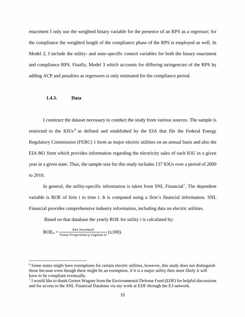
1.4.3. Data

I construct the dataset necessary to conduct the study from various sources. The sample is

restricted to the IOUs 6 as defined and established by the EIA that file the Federal Energy

Regulatory Commission (FERC) 1 form as major electric utilities on an annual basis and also the

EIA 861 form which provides information regarding the electricity sales of each IOU in a given

year in a given state. Thus, the sample size for this study includes 137 IOUs over a period of 2000

to 2010.

In general, the utility-specific information is taken from SNL Financial7. The dependent

variable is ROE of firm i in time t. It is computed using a firm’s financial information. SNL

Financial provides comprehensive industry information, including data on electric utilities.

Based on that database the yearly ROE for utility i is calculated by:

ROEit = 𝑁𝑒𝑡 𝐼𝑛𝑐𝑜𝑚𝑒𝑖𝑡

𝑇𝑜𝑡𝑎𝑙 𝑃𝑟𝑜𝑝𝑟𝑖𝑒𝑡𝑎𝑟𝑦 𝐶𝑎𝑝𝑖𝑡𝑎𝑙 𝑖𝑡 (x100).

6 Some states might have exemptions for certain electric utilities, however, this study does not distinguish

those because even though there might be an exemption, if it is a major utility then most likely it will

have to be compliant eventually. 7 I would like to thank Gernot Wagner from the Environmental Defense Fund (EDF) for helpful discussions

and for access to the SNL Financial Database via my work at EDF through the E3 network.

16

The information on RPS policy in a given state in a given year is taken from the Database

of State Incentives for Renewables and Efficiency (DSIRE)8. It collects information on RPS state

policies as well as the other main energy policies implemented on state level. However, almost all

of the RPS have undergone amendments, so that the information from DSIRE is cross-checked

with the various state-level policies. I collect these information from the PUC and other RPS

related website of each state.

I take the amount of total assets (used as a proxy for the overall utility size) from the SNL

Financial database as well.

The measure for the stringency of the PUC is taken from information provided by the National

Association of Regulatory Utility Commissioners9. Similar to Fremeth and Shaver (2013) this

study uses a binary variable taking the value of 1 if PUC commissioners are directly elected by the

public as a measure for PUC stringency. Lastly, in order to construct the deregulation variable I

use the most recent comprehensive information as of September 2010 provided by the EIA. I weigh

both of the state level variables by the state-specific sales percentage of the utilities. I am using

sales specific information as weights (similar to Fremeth and Shaver (2013), Delmas et al. (2007))

because compliance is usually measured on distribution and not on generation level.

In order to adequately address the main research question of this paper, several estimation

methods could be employed. Given the data structure and thus because of the potential unobserved

utility-specific effects the pooled OLS could result in biased estimators and report wrong standard

errors. Hence, I will further estimate the model using panel data methods; that is a random effects

and a fixed effects model. If the unobserved utility-specific effects are correlated with the

8 Dsireusa.org is a website maintained by the N.C. Solar Center at the N.C. State University. 9 http://www.naruc.org/about.cfm?c=elected [last accessed October 4, 2013].

17

explanatory variables then the fixed effects model should be used in order to get consistent

estimators even though it is less efficient than the random effects model.

1.4.4. Summary Statistics

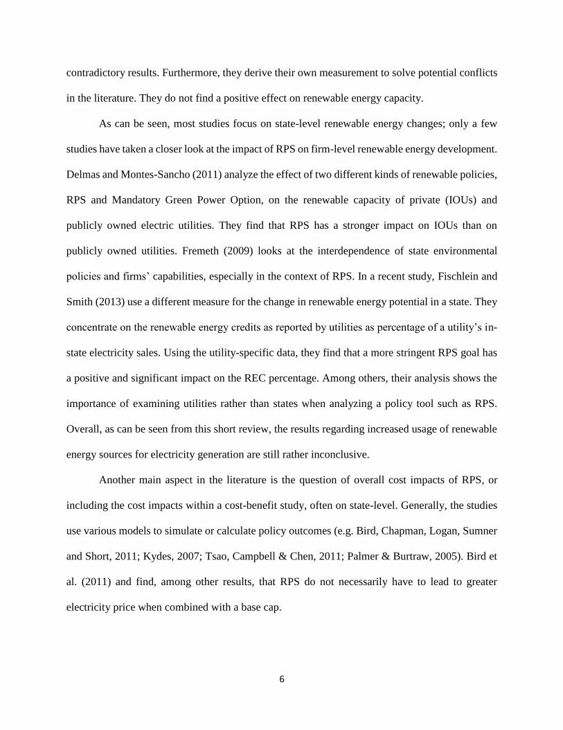
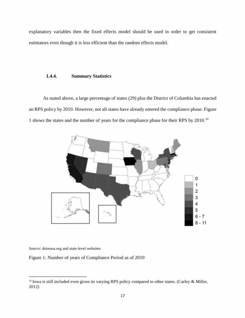
As stated above, a large percentage of states (29) plus the District of Columbia has enacted

an RPS policy by 2010. However, not all states have already entered the compliance phase. Figure

1 shows the states and the number of years for the compliance phase for their RPS by 2010.10

Source: dsireusa.org and state-level websites

Figure 1: Number of years of Compliance Period as of 2010

10 Iowa is still included even given its varying RPS policy compared to other states. (Carley & Miller,

2012)

18

The states with only voluntary goals as of 2010 are not considered as RPS states in this

study.

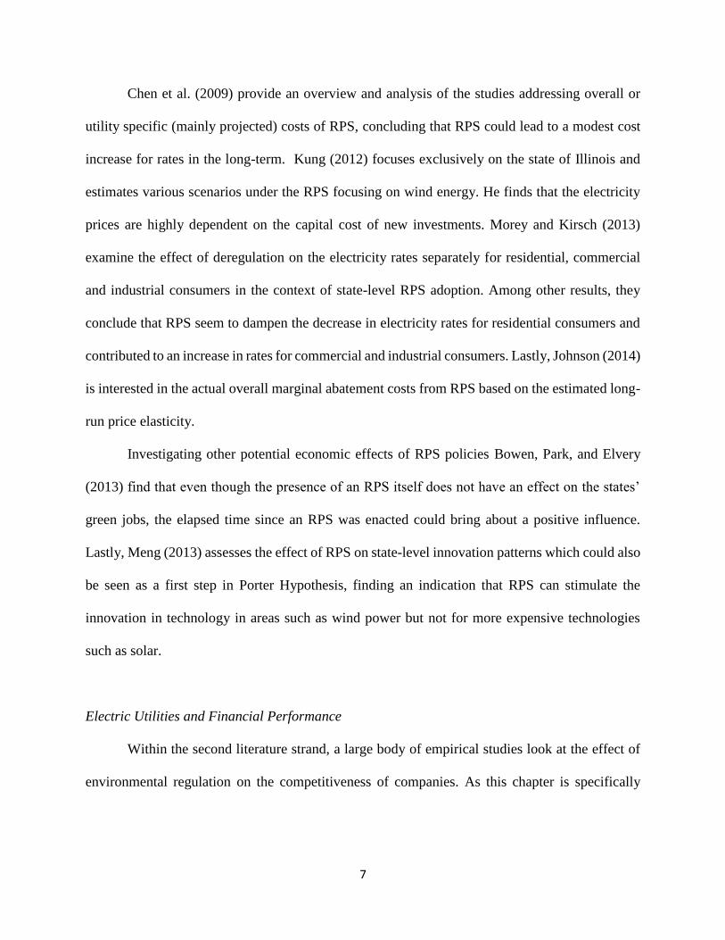
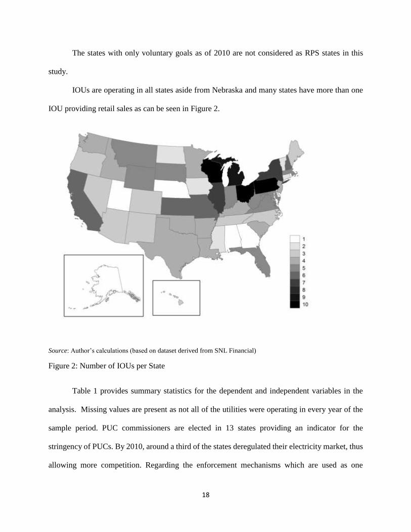
IOUs are operating in all states aside from Nebraska and many states have more than one

IOU providing retail sales as can be seen in Figure 2.

Source: Author’s calculations (based on dataset derived from SNL Financial)

Figure 2: Number of IOUs per State

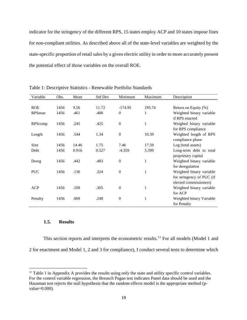
Table 1 provides summary statistics for the dependent and independent variables in the

analysis. Missing values are present as not all of the utilities were operating in every year of the

sample period. PUC commissioners are elected in 13 states providing an indicator for the

stringency of PUCs. By 2010, around a third of the states deregulated their electricity market, thus

allowing more competition. Regarding the enforcement mechanisms which are used as one

19

indicator for the stringency of the different RPS, 15 states employ ACP and 10 states impose fines

for non-compliant utilities. As described above all of the state-level variables are weighted by the

state-specific proportion of retail sales by a given electric utility in order to more accurately present

the potential effect of those variables on the overall ROE.

Table 1: Descriptive Statistics - Renewable Portfolio Standards

Variable Obs. Mean Std Dev Minimum Maximum Description

ROE 1456 9.56 11.72 -174.95 195.74 Return on Equity (%)

RPSenac 1456 .461 .488 0 1 Weighted binary variable

if RPS enacted

RPScomp 1456 .245 .425 0 1 Weighed binary variable

for RPS compliance

Length 1456 .544 1.34 0 10.39 Weighted length of RPS

compliance phase

Size 1456 14.46 1.75 7.46 17.59 Log (total assets)

Debt 1456 0.916 0.527 -4.359 5.399 Long-term debt to total

proprietary capital

Dereg 1456 .442 .483 0 1 Weighted binary variable

for deregulation

PUC 1456 .136 .324 0 1 Weighted binary variable

for stringency of PUC (if

elected commissioners)

ACP 1456 .109 .305 0 1 Weighted binary variable

for ACP

Penalty 1456 .069 .248 0 1 Weighted binary Variable

for Penalty

1.5. Results

This section reports and interprets the econometric results.11 For all models (Model 1 and

2 for enactment and Model 1, 2 and 3 for compliance), I conduct several tests to determine which

11 Table 1 in Appendix A provides the results using only the state and utility specific control variables.

For the control variable regression, the Breusch Pagan test indicates Panel data should be used and the

Hausman test rejects the null hypothesis that the random effects model is the appropriate method (p-

value=0.000).

20

estimation method fits the underlying data structure. First, the Breusch-Pagan test indicates for all

models that the appropriate method is not OLS and that Panel data methods should be used instead.

Secondly, I am using the Hausman test to determine whether a random effects model or a fixed

effects model should be the preferred method. For the parsimonious Model 1, for RPS enactment

and for RPS compliance, the Hausman test fails to reject the null hypothesis that the random effects

model provides consistent estimators. For Model 2 and 3, however, the Hausman test indicates

that the fixed effects estimates are superior to the random effects estimates. Lastly, in that case,

the F-test that all individual utility-specific effects are equal to 0 can be rejected.

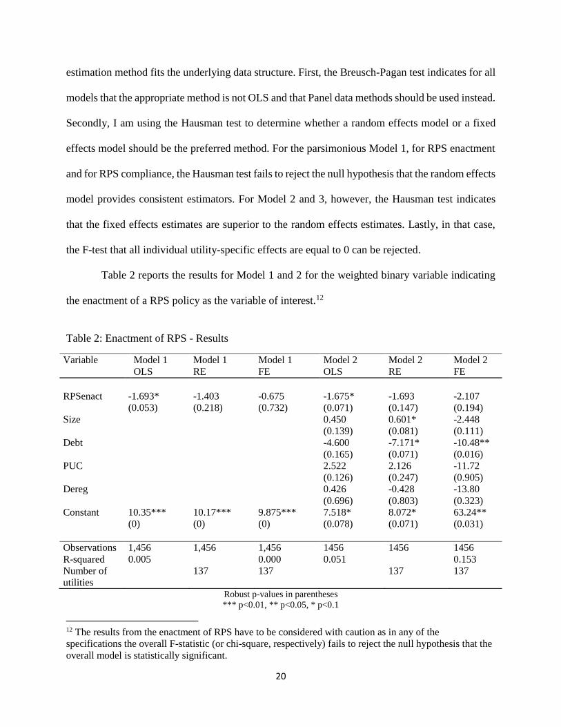
Table 2 reports the results for Model 1 and 2 for the weighted binary variable indicating

the enactment of a RPS policy as the variable of interest.12

Table 2: Enactment of RPS - Results

Variable Model 1

OLS

Model 1

RE

Model 1

FE

Model 2

OLS

Model 2

RE

Model 2

FE

RPSenact -1.693* -1.403 -0.675 -1.675* -1.693 -2.107

(0.053) (0.218) (0.732) (0.071) (0.147) (0.194)

Size 0.450 0.601* -2.448

(0.139) (0.081) (0.111)

Debt -4.600 -7.171* -10.48**

(0.165) (0.071) (0.016)

PUC 2.522 2.126 -11.72

(0.126) (0.247) (0.905)

Dereg 0.426 -0.428 -13.80

(0.696) (0.803) (0.323)

Constant 10.35*** 10.17*** 9.875*** 7.518* 8.072* 63.24**

(0) (0) (0) (0.078) (0.071) (0.031)

Observations 1,456 1,456 1,456 1456 1456 1456

R-squared 0.005 0.000 0.051 0.153

Number of

utilities

137 137 137

137

Robust p-values in parentheses

*** p<0.01, ** p<0.05, * p<0.1

12 The results from the enactment of RPS have to be considered with caution as in any of the

specifications the overall F-statistic (or chi-square, respectively) fails to reject the null hypothesis that the

overall model is statistically significant.

21

The results from the pooled OLS regression provide a first indication that RPS policies

could have a negative impact on the financial performance of IOUs and not as suggested by the

Porter Hypothesis increase their profitability. However, this effect becomes insignificant in the

random effects model, which is the superior choice based on the above described test results. Still,

the coefficient stays negative in sign. When including more control variables, the binary variable

for RPS enactment continues to stay negative, even though it becomes rather insignificant once

again in the panel data model (now the fixed effects model).

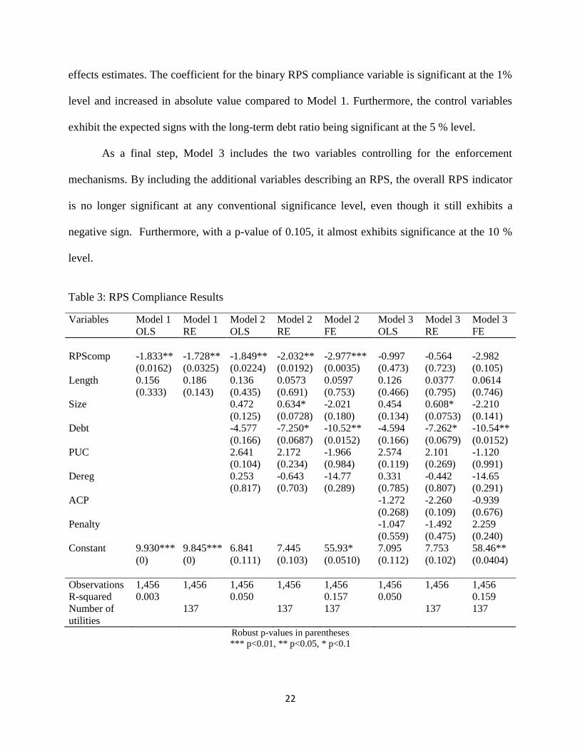
Table 313 reports the results for the three models, now using the weighted binary variable

for the RPS compliance period and the weighted elapsed time since the RPS compliance period

had begun as the main variables of interest. In general, this specification performs better than the

RPS enactment specification as the F-statistic in both fixed effects models (Model 2 and 3)

indicates that the models can be considered statistically significant (p-value=0.034, or p=0.069,

respectively). Similarly, for the random effects estimation for Model 1 the chi-square statistic for

the overall model provides a first indication of statistical significance (p-value=0.0549).

In Model 1 the coefficient for the weighted RPS compliance indicator is negative and

significant at the 5 % level. Even though the length of the compliance period is not significant at

any conventional significance level (p-value=0.143) it exhibits a positive sign which could provide

a first indication that having operated under a RPS system for a longer period of time could

positively affect the financial performance of an IOU as it had time to adjust to the changed policy

environment. In Model 2, the Hausman test had rejected the null hypothesis of consistent random

13 Table 3 does not report the fixe effects for the parsimonious model as the Hausman test identified the

random effects model to be the better choice. The binary variable for RPS is also negative in the fixed

effects model, the number of years positive.

22

effects estimates. The coefficient for the binary RPS compliance variable is significant at the 1%

level and increased in absolute value compared to Model 1. Furthermore, the control variables

exhibit the expected signs with the long-term debt ratio being significant at the 5 % level.

As a final step, Model 3 includes the two variables controlling for the enforcement

mechanisms. By including the additional variables describing an RPS, the overall RPS indicator

is no longer significant at any conventional significance level, even though it still exhibits a

negative sign. Furthermore, with a p-value of 0.105, it almost exhibits significance at the 10 %

level.

Table 3: RPS Compliance Results

Variables Model 1

OLS

Model 1

RE

Model 2

OLS

Model 2

RE

Model 2

FE

Model 3

OLS

Model 3

RE

Model 3

FE

RPScomp -1.833** -1.728** -1.849** -2.032** -2.977*** -0.997 -0.564 -2.982

(0.0162) (0.0325) (0.0224) (0.0192) (0.0035) (0.473) (0.723) (0.105)

Length 0.156 0.186 0.136 0.0573 0.0597 0.126 0.0377 0.0614

(0.333) (0.143) (0.435) (0.691) (0.753) (0.466) (0.795) (0.746)

Size 0.472 0.634* -2.021 0.454 0.608* -2.210

(0.125) (0.0728) (0.180) (0.134) (0.0753) (0.141)

Debt -4.577 -7.250* -10.52** -4.594 -7.262* -10.54**

(0.166) (0.0687) (0.0152) (0.166) (0.0679) (0.0152)

PUC 2.641 2.172 -1.966 2.574 2.101 -1.120

(0.104) (0.234) (0.984) (0.119) (0.269) (0.991)

Dereg 0.253 -0.643 -14.77 0.331 -0.442 -14.65

(0.817) (0.703) (0.289) (0.785) (0.807) (0.291)

ACP -1.272 -2.260 -0.939

(0.268) (0.109) (0.676)

Penalty -1.047 -1.492 2.259

(0.559) (0.475) (0.240)

Constant 9.930*** 9.845*** 6.841 7.445 55.93* 7.095 7.753 58.46**

(0) (0) (0.111) (0.103) (0.0510) (0.112) (0.102) (0.0404)

Observations 1,456 1,456 1,456 1,456 1,456 1,456 1,456 1,456

R-squared 0.003 0.050 0.157 0.050 0.159

Number of

utilities

137 137 137 137 137

Robust p-values in parentheses

*** p<0.01, ** p<0.05, * p<0.1

23

1.6. Conclusion

This chapter addressed the effect of RPS on the financial performance of electric utilities. The

preliminary results seem to indicate a negative relationship between environmental regulation and

the profitability of electric utilities. Thus, they appear to reject the Porter Hypothesis and generally

support the results found in the literature on the effect of environmental regulation on the financial

performance in the electricity sector.

A few notes of caution should be kept in mind when interpreting the results. First of all, RPS

are still a fairly recent policy device to increase the usage of renewable energy sources for

electricity. Given that that the elapsed time since the first compliance year as of 2010 is rather

short for some states, electric utilities might not have had time to adjust.14 Investments in the

electricity sector are rather long-term. Hence, the results presented need not reflect long-run effects.

Second, as discussed by Stockmayer et al. (2012), the enforcement measures are often coupled

with cost recovery mechanisms for the electric utility, as well as potential waivers to compliance

requirements. Operating in such a low enforcement environment is not necessarily in accordance

with the assumptions of the Porter Hypothesis which stipulates that environmental policies must

be stringent yet flexible. Third, even though this study tries to be as thorough as possible, it is still

using rather coarse measures to capture the stringency of RPS policies by employing sales-

weighted dummies as the main indicators. Lastly, this study focuses on IOUs operating in

individual states as measured by their total retail electricity volume. A next step is to focus on the

generational aspect of electric utilities as RPS policies must increase the generation of electricity

from renewable energy sources in order for the policies to support the Porter Hypothesis.

14 As Barbose, Wiser, Phadke & Goldman (2008) point out, utilities try to prepare for future carbon

negotiations using various strategies in advance. Still, it could take time for the investment to pay off or

be effective.

24

2. The Influence of Environmental Management Practices on

Compliance with Effluent Limits

2.1. Introduction

Since the early 1970s the use of performance-based standards, sometimes incorrectly classified

as the command-and-control approach, has been the prevalent choice for governments around the

world to improve and protect air and water quality. In the United States, the Clean Water Act

(CWA) uses performance-based standards to protect surface water quality. The Environmental

Protection Agency (EPA) controls most of the CWA regulatory aspects through the National

Pollutant Discharge Elimination System (NPDES). As the starting point of the NPDES

implementation every facility that has point-source discharges needs to possess an effluent permit.

These permits regulate wastewater pollutant discharges mainly by establishing limits on the

allowable amount of the pollution.

These effluent limits represent performance-based standards, which place restrictions only on

the amount of pollution. They do not require any specific approaches for controlling discharges.

Instead, within this regulatory context, facilities are free to adopt a variety of environmental

management practices for controlling their discharges. When organized as a package, these various

practices represent an Environmental Management System (EMS). An Environmental

Management System may be monitored and certified by a third party. ISO 14001 certification

represents one example. While these environmental management practices – organized as a system

or not, certified or not – may serve to comply with effluent limits, these practices frequently serve

to over-comply with effluent limits. In this sense, these environmental management practices are

also voluntary in nature, i. e. not needed in order to comply with required effluent limits. Clearly,

if environmental management practices facilitate compliance, if not over-compliance, their use

25

should reduce the burden of enforcement costs imposed on facilities by the part of regulatory

agencies. However, these positive results follow only if the facilities’ environmental management

practices indeed lower discharges. Given the potential benefits of environmental management

systems the EPA has promoted their use by regulated companies in order to improve

environmental performance, especially the use of self-audits (Evans, Liu & Stafford., 2011).

Several studies have examined the effect of self-audits on compliance (Evans et al., 2011; Khanna

& Widyawati, 2011; Earnhart & Harrington, 2013).

In contrast, this chapter contributes to the existing literature on EMS and environmental

performance by examining the effect of the arguably first step in facilities’ reduction efforts on

their discharges. Specifically, I will focus on internal monitoring actions as one type of

environmental management practice undertaken by chemical manufacturing facilities regulated

under the Clean Water Act. Although any environmental management effort could be expected to

lower discharges, the main interest of this paper is internal monitoring effort since it is easier to

control pollution after assessing where pollutants are created within the production process and

how well they are treated in the treatment process, thus improving the facility’s ability to control

pollution.

Furthermore, similar to Earnhart and Harrington (2013), I do not only examine whether the

regulated facilities in the sample are in compliance or not but rather look at the level of compliance

and potential over-compliance. I am able to do so by using the ratio of actual pollution (in the form

of discharges) to the level of pollution as permitted by the EPA. This discharge ratio allows me to

measure the effect of internal monitoring on the extent of compliance.

In order to address the importance of internal monitoring on the reduction of discharges this

chapter exploits panel data. In addition, the econometric analysis addresses the potential

26

endogeneity of internal monitoring, since it clearly represents a choice variable, along with some

other explanatory variables, as described in Section 3.

The remainder of the chapter is organized as follows. Section 2 provides a review of the related

literature. Section 3 provides a basic conceptual framework. Section 4 describes the econometric

framework used in the analysis, including the data necessary. Section 5 presents the estimation

results. Section 6 concludes.

2.2. Literature Review

This paper draws mainly from two kinds of literature strands; adoption of environmental

management practices undertaken by firms and (over-) compliance with environmental regulations.

As explained above, I consider environmental management actions of firms to be voluntary in the

sense that they are not required by law even though firms need to comply with environmental

regulations. The often resulting over-compliance can thus be considered as a voluntary behavior.

Adoption of environmental management practices

Several papers within this literature are concerned with the reasons why a firm would

choose to adopt environmental management practices and in a second step the effect it has on their

emissions. These management practices can either be within pure voluntary programs sponsored

by a government or also within a strict regulatory setting.

Numerous papers (e.g. Harrington, Khanna & Deltas, 2008; Khanna, Deltas & Harrington.,

2009; Uchida & Ferraro, 2007; Johnstone & Labonne, 2009) focus on the motivation for firms to

adopt environmental management techniques, either in a certified setting or as a count of pollution

abatement technologies (Khanna et al., 2009).

27

In particular, Harrington et al. (2008) conclude that the implementation of a Total Quality

Environmental Management (TQEM) is mainly driven by internal factors whereas Johnstone and

Labonne (2009) additionally contribute the stringency of environmental regulations to which firms

are subject and the regulatory advantage they hope to gain from environmental management

systems to the adoption.

Other papers such as Arimura, Hibiki and Katayama (2008), Barla (2007), Hertin, Wagner

and Tyteca (2008) concentrate on the effect of environmental management practices on

environmental performance with varying results. Barla (2007) finds no significant reduction in

TSS emissions for plants in the pulp and paper industry in Quebec. In contrast, Arimura et al.

(2008) see a positive effect of the adoption of ISO 14001 on the environmental performance of

companies in Japan.

Sam, Khanna and Innes (2009) look at the effectiveness of voluntary approaches in the

setting of the 33/50 program. In particular, they examine if such a program increases the incentive

for firms to adopt a TQEM and if this adoption leads to a short and long-term reduction of

emissions. As a result they state that the participation in the 33/50 program tends to incentivize the

adoption of TQEM which helps to reduce the 33/50 releases. Similar, Innes and Sam (2008) find

that the participation in 33/50 program is more likely from firms with higher rates of governmental

regulations as they might see a reduction in inspections after they joined. Once again the adoption

of the voluntary program reduces emissions.

Compliance and Over-compliance literature

Previous studies examine the effect of environmental management practices on pollution

levels. For example, Anton, Deltas and Khanna (2004) analyze potential factors that encourage

28

firms to adopt environmental management systems, which include multiple components such the

number of environmental staff, presence of a written environmental policy, and the presence or

count of self-audits; and then investigate the effect of these on the emission of hazardous air

pollutants. However, the authors use only cross-sectional data. In contrast, Sam et al. (2009) use

panel data to examine the impact of the adoption of a total quality management program on the

emissions of 33/50 pollutants in the 1990s. They find that this adoption has a significantly negative

effect on the 33/50 emissions.

Stafford (2002) analyzes the effect of the revision of the penalty policy of the EPA on

compliance regarding hazardous waste regulations. Using a bivariate probit model with

inspections and violations as the dependent variable she finds that most factors that increase the

probability of violations also increase the probability of inspections. Furthermore, the change in

the penalty policy did indeed increase the compliance even though to a much lesser degree. Telle

(2008) analyzes the behavior of firms under threats of violations, finding that the threat of

inspections reduces the probability of violations of firms. Also looking at the effect of regulatory

measures, Shimshack and Ward (2005) analyze the importance of enforcement on compliance.

They conclude that the impact of sanctions on other plants is almost as strong as the impact on the

plant subject to sanctions.

Shimshack and Ward (2008) look at the effect of regulatory enforcement on the ratio of

actual BOD or TSS discharges to legally permitted level for plants in the pulp and paper industry

finding that enforcement actions by a regulatory agency leads to increased over-compliance of

plants. This chapter looks at a similar set of facilities and their compliance levels. However, the

variable of interest, internal monitoring, can be considered as a first step to an environmental

29

management system and thus connects the literature of environmental management and over-

compliance.

Other papers which also connect environmental management and compliance are for

example Potoski and Prakash (2005) analyzing how ISO 14001 improves compliance and Khanna

and Widyawati (2011). They examine the effect of one environmental management technique,

self-audits, on the compliance using a probit model with the dependent variable being an indicator

for compliance of a firm in a given time period and find that firms that self-audit are more likely

to be compliant with Clean Air Act regulations. They also derive theoretically and empirically the

motivation for a firm to self-audit.

Similarly, instead of looking at a comprehensive environmental management system, this

chapter analyzes the effect of one fundamental non-mandatory environmental practice which could

be considered to be the first step towards an environmental management system.

2.3. Conceptual Framework

Similar to Shimshack and Ward (2007), I consider a rational decision making firm that will

only choose to implement additional abatement technology until the marginal benefit from such

technology equals its marginal cost. Monitoring technology which is not legally required always

constitutes an added cost for the firm. However, the cost for the firm could be much higher if it is

not in compliance with the legally set limits and if this non-compliance is detected by the

regulatory agency. As Shimshack and Ward (2007) point out, over-compliance can also be

explained by firms trying to provide a certain safety against stochastic shocks to ensure compliance

and avoid any regulatory costs. A firm would choose to implement additional monitoring

technologies in order to be able to control its own treatment process more effectively and thus

30

reduce its discharges. Given the importance for facilities to stay in compliance as found in previous

literature, it can be assumed that most facilities will implement monitoring technology within the

treatment process and not just the required monitoring technology outside the treatment process.

Hence, I hypothesize, that the best monitoring technology will decrease discharges to a higher

degree than the others.

Hypothesis 1: A more sophisticated monitoring technology will lead to a higher reduction

of discharges.

The regulatory framework is uncertain, that is, a facility does not necessarily know when it

will face an inspection and if it is non-compliant, a fine. The political environment is constantly

changing, so the effluent limits might be changing as well. Hence, a facility will base its decisions

regarding discharges on its own previous experience and the experience of other facilities in the

same state (see for example Shimshack and Ward (2008), Earnhart, (2009)).

Hypothesis 2: Increased inspections and enforcement actions experienced by facilities

within the same state will cause a facility to become more cautious and reduce its

discharges even if it is already compliant.

Lastly, I also expect regulatory pressure put on a facility to have a strong effect on the discharges

by that facility.

Hypothesis 3: Increased inspections and enforcement actions experience by a facility

itself will cause the facility make certain to stay compliant and thus reduce its discharges.

The next section describes the formulation of the econometric framework as well as the data

collection and the data itself.

31

2.4. Econometric Framework and Methods

This section translates the conceptual framework into the empirical setting which is used for

the analysis. In addition, it discusses the empirical method, panel data, used for the analysis in

greater detail.

2.4.1. Econometric Framework

Effluent limits place legal constraints on facilities’ discharges. However, facilities need not

exactly comply with these limits. Some facilities may prefer to exceed their limits while running

the risk of increased inspection scrutiny and the imposition of sanctions (e.g., fines). Other

facilities may over-comply due to non-regulatory benefits (e.g., better reputation). To capture this

variation, this chapter employs a measure of the actual level of discharges relative to the permitted

level of discharges, hereafter the discharge ratio.

Several factors may influence facilities’ decisions regarding this discharge ratio. I focus

on the influence of environmental management practices. In particular, I examine the effect of a

single practice, internal monitoring, which can vary greatly in its extent from facility to facility.

All permitted facilities are required to implement end-of-pipe monitoring as part of their reporting

to regulatory agencies. Some facilities may choose not to implement any additional monitoring

beyond this required monitoring. Other facilities may elect to monitor internally prior to the end-

of-pipe discharge. If facilities decide to monitor internally, they may employ a basic in-stream

monitoring protocol within the treatment process. More sophisticated internal monitoring

protocols also include single-point or multiple-point sewer monitoring, in addition to treatment

32

process monitoring. These more sophisticated protocols monitor the production process itself at a

single point or multiple points; they are aimed at pollution prevention.

The set of explanatory variables also includes various measures of interventions taken by

regulators. First, state and federal environmental agencies conduct inspections, which enhance the

regulatory pressure placed on facilities to comply with the imposed effluent limits. I anticipate

that inspections affect facilities’ decisions with a lag because facilities need time to adjust their

discharges. Accordingly, I include lagged inspections as the relevant regressor in the econometric

model. Rather than constraining my exploration to a single preceding time period, I count all of

the inspections (state and federal) conducted over the 12-month period preceding the current month

of discharges in order to form a single regressor.

Second, similar to inspections, regulatory agencies take enforcement actions in order to

induce compliance. In particular, agencies take two kinds of enforcement actions that should

induce facilities to comply: (1) formal enforcement actions, such as consent decrees, and (2)

informal enforcement actions, such as notices of noncompliance. As with inspections, it can be

anticipated that enforcement actions influence facilities’ decisions with a lag since facilities need

time to respond to enforcement actions. I include the count of preceding enforcement actions taken

over the preceding 12-month period as a single regressor.

This chapter examines both types of interventions – inspections and enforcement actions –

in two forms. As the first form, the influence of lagged inspections and enforcement actions on

discharge decisions represents specific deterrence. As the second form, a facility may also be

influenced by general deterrence, which stems from inspections conducted at and enforcement

actions taken against other facilities, i.e., facilities in “general”. This general deterrence is captured

by measuring the interventions taken against other similar facilities – based on the broad economic

33

sector -- in the same state or EPA region, as relevant, in a particular calendar year. Assuming that

facilities are aware of these interventions against other similar facilities, this awareness of other

facilities having faced inspections or enforcement actions increases the perceived probability that

the specific facility may be subject to similar regulatory pressure might induce the facility to

improve its environmental performance, i.e., lower its discharge ratio.

The set of explanatory variables also includes control factors. First, I control for facility

size using the number of employees as a proxy. Second, I control for temporal variation over the

different years of the sample – 2001, 2002, and 2003 – by including year indicators for 2002 and

2003, with 2001 serving as the benchmark year, as regressors. In addition, the analysis controls

for seasonal effects by including dummy variables for three of the four seasons based on these sets

of months: winter (January, February, March); spring (April, May, June); and summer (July,

August, September); with autumn serving as the benchmark season. I also control for spatial

variation across the different 10 EPA regions. Lastly, I control for sectoral variation across the

subsectors within the broad sector of chemical manufacturing by including indicator variables for

the organic chemicals and inorganic chemicals sub-sector, with “other chemicals” serving as a

benchmark category.

Based on the above description the following notation is defined. Let Dit represent the

discharge ratio. Let Mi represent internal monitoring. Let Iit represent the government intervention

measures. Let Xit represent a matrix of control variables, such as season and year. Given this

notation, I construct the econometric equation as the following:

Dit = α+ MiT δ + Dit

Tβ1+ XitTβ2+ εit,

where εit, decomposes into the sum of μi and uit, with μi being the individual facility-specific

unobserved effect, which is time-invariant, and uit being the facility- and time-specific error term.

34

2.4.2. Econometric Methods

In the following, this basic equation is estimated according to three different models. Model A

uses for the main variable of interest – internal monitoring – a four level monitoring variable (no

monitoring, treatment process monitoring, treatment process monitoring and single point sewer

monitoring, and treatment process monitoring and multiple points sewer monitoring). For Model

B, I create a binary variable that takes the value of 1 if the facility has chosen to implement

multiple-points sewer monitoring and 0 otherwise. It seems more meaningful to divide the sample

into these two groups than into for example no monitoring versus any monitoring because only 5%

of the facility in the sample chose not to implement any monitoring technologies. Further testing

shows that the chosen division of the variables is meaningful. This test is accomplished within

Model C (as described below) which has binary variables for each level of monitoring (“no

monitoring” being the omitted category). This model also gives me the opportunity to test whether

the two intermediate levels (“treatment process monitoring only” and” treatment process

monitoring plus single-point sewer monitoring”) jointly equal zero.

Finally, Model C probably provides the most accurate division of the monitoring variable; i.

e. it includes a binary variable for each of the different levels of monitoring technology with ‘no

monitoring’ being the benchmark variable.

Given these three models (A, B and C) I wish to estimate the relationship between discharges

and a set of explanatory variables, with internal monitoring as my key variable of interest. In my

sample, internal monitoring is time-invariant. If the unobserved facility-specific effects identified

in the estimation equation were not present, I could estimate the regression equation using pooled

35

OLS so the time-invariance of internal monitoring is not problematic. If the explanatory variables

are uncorrelated with the unobservable facility-specific effects, then the random effects estimator

generates consistent results so again the time-invariance of internal monitoring is not binding.

However, if the explanatory variables are correlated with the unobservable facility-specific effects,

then the random effects estimator generates inconsistent results. In this case, the fixed effects

estimator proves the most obvious choice of analysis. Regrettably, a fixed effects estimator does

not provide any meaningful results for my purposes since the estimator cannot analyze time-

invariant variables. Fortunately, I demonstrate below that the random effects estimates appear

consistent in all considered cases. I also provide results from the Hausman-Taylor estimation of

the above described model which has the added advantage that time-invariant variables can still

be included in a fixed effects regression as further described below.

As a second concern, I am aware of the potential endogeneity of my variable of interest

monitoring. Thus, I also test for potential endogeneity of internal monitoring. I use as instruments

lagged intervention variables, specifically state and federal inspections variables measured with

an additional time lag of 24 months. More greatly lagged interventions should influence a facility’s

internal monitoring decision, especially since facilities need time to establish an internal

monitoring protocol in response to government interventions, while not having an independent

effect on the currently chosen discharge ratio. Thus, more greatly lagged interventions could

constitute useful instruments in the cases where internal monitoring is indeed endogenous.

36

2.4.3. Data Description

The data on facilities were compiled from different sources. The facilities in this study are all

major actors in the chemical manufacturing sector. They are regulated under the Clean Water Act

and granted permission to discharge through the National Pollutant Discharge Elimination System

(NPDES) by the EPA. As described in detail by Earnhart and Harrington (2013), the limit values

for pollutants regulated under the Clean Water Act vary across facilities and across time even

within the same sector. Hence, for this analysis, I will also use the discharges relative to the

permitted limits for each facility and not only the absolute discharge value. In order to assess the

compliance, the EPA requires facilities to report their discharges using Discharge Monitoring

Reports. These data are publicly available.

Hence, the data on discharges and permit limits as well as on inspections and enforcement

actions are taken from the publicly accessible EPA’s Permit Compliance System (PCS) database

which were available only for major facilities. Finally, limits are pollutant specific. Thus, this

chapter only focuses on facilities discharging Total Suspended Solids (TSS), one of the main

pollutants under the CWA, so that the sample size is 76 facilities that have either concentration or

quantity limits, measured in mg/L or lbs/day respectively. Given my data, focusing on TSS will

give me the largest possible sample.

Facility-specific data was gathered through a survey conducted between March 2002 and

March 2003. The survey population consisted of the full sample of 2,596 facilities from the EPA’s

PCS database (as of September 2001). This survey population was reduced to 1003 facilities based

on whether the facility had a NPDES permit, faced restrictions on their discharges and discharged

into surface water, was operating in 2002, and contact information was available (Earnhart &

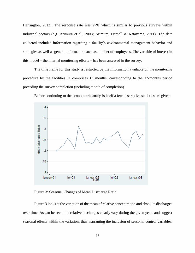
37

Harrington, 2013). The response rate was 27% which is similar to previous surveys within

industrial sectors (e.g. Arimura et al., 2008; Arimura, Darnall & Katayama, 2011). The data

collected included information regarding a facility’s environmental management behavior and

strategies as well as general information such as number of employees. The variable of interest in

this model – the internal monitoring efforts – has been assessed in the survey.

The time frame for this study is restricted by the information available on the monitoring

procedure by the facilities. It comprises 13 months, corresponding to the 12-months period

preceding the survey completion (including month of completion).

Before continuing to the econometric analysis itself a few descriptive statistics are given.

Figure 3: Seasonal Changes of Mean Discharge Ratio

Figure 3 looks at the variation of the mean of relative concentration and absolute discharges

over time. As can be seen, the relative discharges clearly vary during the given years and suggest

seasonal effects within the variation, thus warranting the inclusion of seasonal control variables.

38

Furthermore, the relative discharges vary within the range of 0 to 1 indicating that on a monthly

mean the facilities stayed in compliance with their permit limits.

Table 4 gives summary statistics for the different variables. Generally, the sample size

might seem small; however, it represents a wide range of facilities. The number of employees,

which is the proxy of facility size alone ranges from 7 to 1600 with a mean around 350. Chemical

manufacturing facilities in the inorganic sector are slightly overrepresented with 60%, but the

organic sector is as well strongly represented (20%).

The overall mean of the dependent variable shows a general over-compliance of the

facilities within the given permit values although there do exist facilities that did not stay within

their permit limits in a certain month. In particular, the average facility discharges at three fourth

below its allowed permit limit.

The mean values for the different count values for the deterrence measures from regulatory

agencies indicate low regulatory pressure. For example, the mean value for the sum of state and

federal inspections at one facility in the preceding 12 month period is less than 2 inspections. The

mean value for specific enforcement actions in the same time frame is 0.32.

Regarding the main variable of interest, internal monitoring, more than half of the facilities

in the sample have a “higher” standard of internal monitoring and only 5 % opt out of additional

monitoring completely. Even though most facilities do adopt some kind of monitoring technology

I still think it is important to know if a more sophisticated and thus more expensive monitoring

technology can lower the final discharges and thus prove the usefulness of such technology.

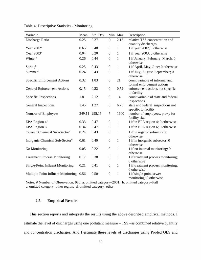
39

Table 4: Descriptive Statistics - Monitoring

Variable Mean Std. Dev. Min Max Description

Discharge Ratio 0.25 0.27 0 2.13 relative TSS concentration and

quantity discharges

Year 2002a 0.65 0.48 0 1 1 if year 2002; 0 otherwise

Year 2003a 0.04 0.20 0 1 1 if year 2003; 0 otherwise

Winterb 0.26 0.44 0 1 1 if January, February, March; 0

otherwise

Springb 0.25 0.43 0 1 1 if April, May, June; 0 otherwise

Summerb 0.24 0.43 0 1 1 if July, August, September; 0

otherwise

Specific Enforcement Actions 0.32 1.83 0 21 count variable of informal and

formal enforcement actions

General Enforcement Actions 0.15 0.22 0 0.52 enforcement actions not specific

to facility

Specific Inspections 1.8 2.12 0 14 count variable of state and federal

inspections

General Inspections 1.45 1.27 0 6.75 state and federal inspections not

specific to facility

Number of Employees 349.11 295.15 7 1600 number of employees; proxy for

facility size

EPA Region 4c 0.33 0.47 0 1 1 if in EPA region 4; 0 otherwise

EPA Region 6c 0.34 0.47 0 1 1 if in EPA region 6; 0 otherwise

Organic Chemical Sub-Sectord 0.24 0.43 0 1 1 if in organic subsector; 0

otherwise

Inorganic Chemical Sub-Sectord 0.61 0.49 0 1 1 if in inorganic subsector; 0

otherwise

No Monitoring 0.05 0.22 0 1 1 if no internal monitoring; 0

otherwise

Treatment Process Monitoring 0.17 0.38 0 1 1 if treatment process monitoring;

0 otherwise

Single-Point Influent Monitoring 0.21 0.41 0 1 1 if treatment process monitoring;

0 otherwise

Multiple-Point Influent Monitoring 0.56 0.50 0 1 1 if single-point sewer

monitoring; 0 otherwise

Notes: # Number of Observation: 980. a: omitted category=2001, b: omitted category=Fall

c: omitted category=other region, d: omitted category=other

2.5. Empirical Results

This section reports and interprets the results using the above described empirical methods. I

estimate the level of discharges using one pollutant measure – TSS –as combined relative quantity

and concentration discharges. And I estimate these levels of discharges using Pooled OLS and

40

Panel Data methods. Based on these estimators, I perform tests to assess whether each set is

unbiased and consistent. I first test whether the random effects estimates dominate the pooled OLS

estimates based on the Breusch-Pagan test. I next test whether the random effects estimates are

consistent based on a comparison with the fixed effects estimates using the Hausman test for

random effects. If consistent, the random effects dominate the fixed effects estimates since the

former estimates are more efficient and provide effects of time-invariant factors.

2.5.1. Main Results

Table 5 reports the results using the 4-level (no monitoring, treatment process monitoring,

single-point sewer monitoring and multiple-points sewer monitoring) discrete monitoring variable.

I first show the results from the basic regression by just including the time-varying and time-

invariant control variables before having the full set of deterrence measures as exogenous variables.

This basic regression uses OLS to show the main trend behind the monitoring effect. The Breusch-

Pagan test indicates that the underlying structure of the data is indeed the panel format and pooled

OLS is not the appropriate method. Therefore, I also use the random effects method. In both

methods I cluster on individual facilities. The variable of interest stays significant at the 5 % level

and exhibits the expected negative sign in all of the specifications. So, it seems that the higher the

level of the internal monitoring the lower the discharges. Additionally, the regulatory pressure

seems to induce facilities to lower their discharges with the facility-specific enforcement actions

being significant in the pooled OLS regression at the 10% level and significant at the 5% level in

the random effects model, thus meeting the expectations from the environmental agencies.

Furthermore, the type of production process seems to be relevant for the discharges by a facility.

41

Chemical manufacturing facilities within the ‘inorganic’ sector seem to have higher discharge

ratios than facilities in ‘other’ categories; the coefficient indicating the ‘organic’ sector is also

positive, however, not significant at any conventional significance level. Lastly, the Hausman test

reports a p-value of 0.1904, thus failing to reject the null hypothesis that the random effects model

provides consistent estimates. Hence, in this case the random effects estimation is the appropriate

panel data method.

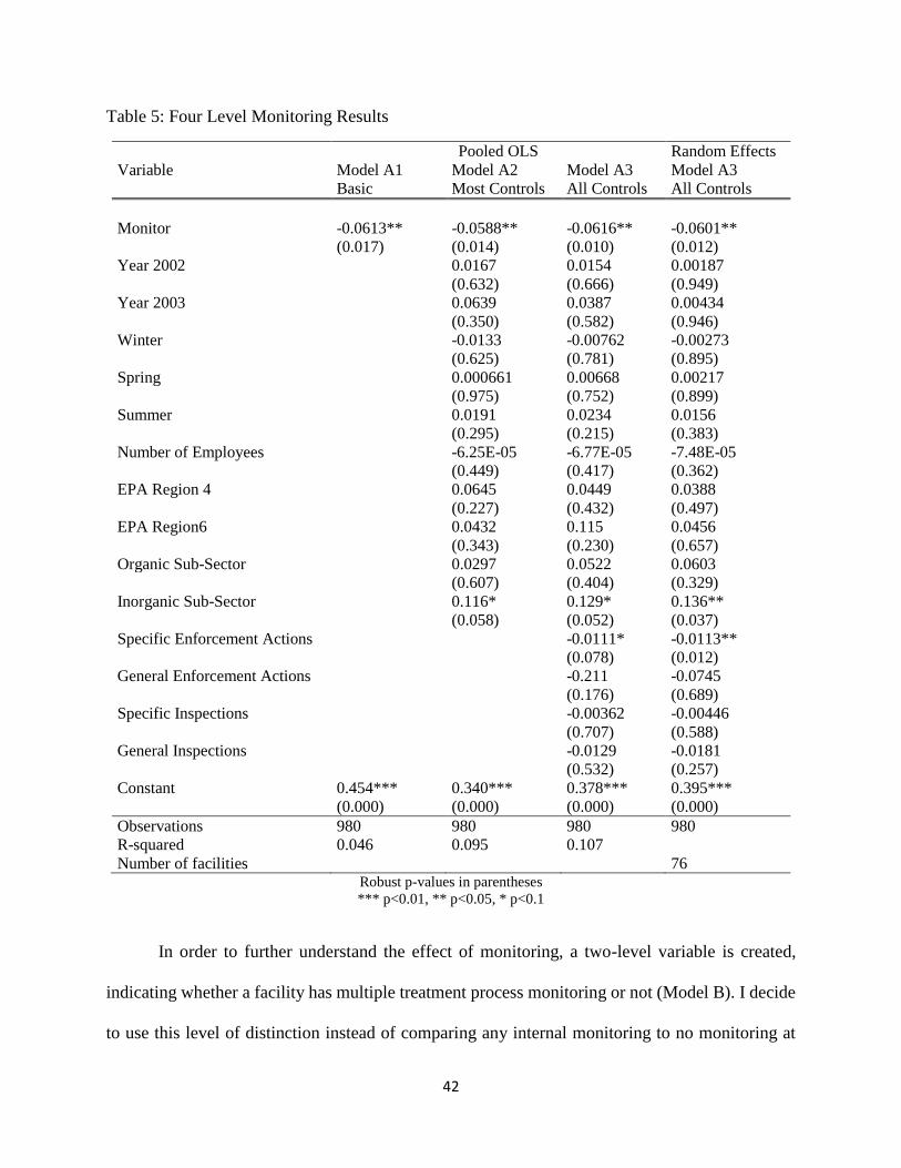
42

Table 5: Four Level Monitoring Results

Pooled OLS Random Effects

Variable Model A1

Basic

Model A2

Most Controls

Model A3

All Controls

Model A3

All Controls

Monitor -0.0613** -0.0588** -0.0616** -0.0601**

(0.017) (0.014) (0.010) (0.012)

Year 2002 0.0167 0.0154 0.00187

(0.632) (0.666) (0.949)

Year 2003 0.0639 0.0387 0.00434

(0.350) (0.582) (0.946)

Winter -0.0133 -0.00762 -0.00273

(0.625) (0.781) (0.895)

Spring 0.000661 0.00668 0.00217

(0.975) (0.752) (0.899)

Summer 0.0191 0.0234 0.0156

(0.295) (0.215) (0.383)

Number of Employees -6.25E-05 -6.77E-05 -7.48E-05

(0.449) (0.417) (0.362)

EPA Region 4 0.0645 0.0449 0.0388

(0.227) (0.432) (0.497)

EPA Region6 0.0432 0.115 0.0456

(0.343) (0.230) (0.657)

Organic Sub-Sector 0.0297 0.0522 0.0603

(0.607) (0.404) (0.329)

Inorganic Sub-Sector 0.116* 0.129* 0.136**

(0.058) (0.052) (0.037)

Specific Enforcement Actions -0.0111* -0.0113**

(0.078) (0.012)

General Enforcement Actions -0.211 -0.0745

(0.176) (0.689)

Specific Inspections -0.00362 -0.00446

(0.707) (0.588)

General Inspections -0.0129 -0.0181

(0.532) (0.257)

Constant 0.454*** 0.340*** 0.378*** 0.395***

(0.000) (0.000) (0.000) (0.000)

Observations 980 980 980 980

R-squared 0.046 0.095 0.107

Number of facilities 76 Robust p-values in parentheses

*** p<0.01, ** p<0.05, * p<0.1

In order to further understand the effect of monitoring, a two-level variable is created,

indicating whether a facility has multiple treatment process monitoring or not (Model B). I decide

to use this level of distinction instead of comparing any internal monitoring to no monitoring at

43

all. This division is not only more meaningful given the fact that more facilities decided to have

such a high level of internal monitoring than no monitoring at all, I also test separately for the

coefficients of treatment process monitoring and single-point sewer monitoring to be different

from zero. I fail to reject the null hypothesis that these two coefficients are equal to zero (p-value=

0.449) and feel confident that my two-level variable provides a good indicator for internal

monitoring. The results are presented in Table 6. Once again, the variable for internal monitoring

exhibits the expected negative sign and stays significant at the 5% (10% in the basic regression)

level throughout the different specifications. The Breusch-Pagan test indicates that panel data

methods should be used and the Hausman test fails to reject the null hypothesis that the random

effects model is consistent with a p-value of 0.3050. The coefficients for the deterrence measures

are all negative with the specific enforcement actions being significant. This indicates that facilities

that either have been subject to inspections or any kind of formal or informal enforcement actions

or facilities observing the fact that other facilities are subject enforcement actions, have an

incentive to lower their discharges. Similarly to Model A, facilities in the inorganic sector seem to

have higher discharges than in other sectors.

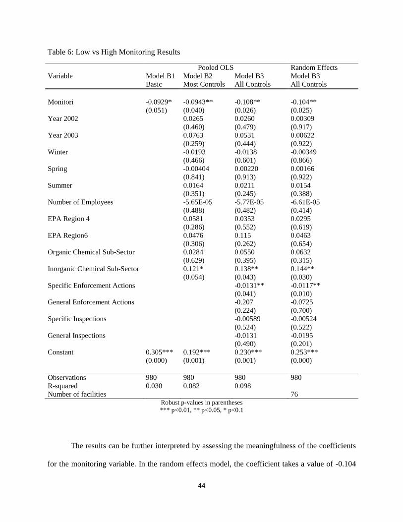
44

Table 6: Low vs High Monitoring Results

Pooled OLS Random Effects

Variable Model B1

Basic

Model B2

Most Controls

Model B3

All Controls

Model B3

All Controls

Monitori -0.0929* -0.0943** -0.108** -0.104**

(0.051) (0.040) (0.026) (0.025)

Year 2002 0.0265 0.0260 0.00309

(0.460) (0.479) (0.917)

Year 2003 0.0763 0.0531 0.00622

(0.259) (0.444) (0.922)

Winter -0.0193 -0.0138 -0.00349

(0.466) (0.601) (0.866)

Spring -0.00404 0.00220 0.00166

(0.841) (0.913) (0.922)

Summer 0.0164 0.0211 0.0154

(0.351) (0.245) (0.388)

Number of Employees -5.65E-05 -5.77E-05 -6.61E-05

(0.488) (0.482) (0.414)

EPA Region 4 0.0581 0.0353 0.0295

(0.286) (0.552) (0.619)

EPA Region6 0.0476 0.115 0.0463

(0.306) (0.262) (0.654)

Organic Chemical Sub-Sector 0.0284 0.0550 0.0632

(0.629) (0.395) (0.315)

Inorganic Chemical Sub-Sector 0.121* 0.138** 0.144**

(0.054) (0.043) (0.030)

Specific Enforcement Actions -0.0131** -0.0117**

(0.041) (0.010)

General Enforcement Actions -0.207 -0.0725

(0.224) (0.700)

Specific Inspections -0.00589 -0.00524

(0.524) (0.522)

General Inspections -0.0131 -0.0195

(0.490) (0.201)

Constant 0.305*** 0.192*** 0.230*** 0.253***

(0.000) (0.001) (0.001) (0.000)

Observations 980 980 980 980

R-squared 0.030 0.082 0.098

Number of facilities 76 Robust p-values in parentheses

*** p<0.01, ** p<0.05, * p<0.1

The results can be further interpreted by assessing the meaningfulness of the coefficients

for the monitoring variable. In the random effects model, the coefficient takes a value of -0.104

45

and is significant at the 5% level, indicating that multiple sewer monitoring decreases the

discharges by -0.104 compared to any of the other monitoring technologies (including no

monitoring at all). The mean value of TSS quantity and concentration discharge ratio is 0.25 (see

Table 4). When comparing the coefficient for the monitoring indicator in the discharge ratio to

the mean value, the coefficient of -0.104 represents a 41.6% reduction of discharges, clearly

indicating the importance internal monitoring technology can have on the amount of discharges

for a facility and as such the potential of reduction of regulatory costs.

As a final specification I also present results in Table 1 in Appendix B where I use the different

levels of internal monitoring with having no monitoring as the benchmark (Model C). Once again,

the Breusch-Pagan test indicates that panel data methods should be used and the Hausman tests

fails to reject the null hypothesis (p-value=0.2234). Hence, the random effects model is used.

Even though the results are not significant, the different levels of monitoring have negative

coefficients which are increasing in absolute value as the internal monitoring process becomes

technically more advanced. This last result is similar to Barla (2007), who cannot find strong

evidence regarding negative influence of the (voluntary) ISO 14001 adoption on the TSS and

discharges in Quebec's pulp and paper industry. The specific enforcement actions and the control

variable for the inorganic sector prove to be significant again, having the same effect on the TSS

discharge ratio as in Model A and B.

46

2.5.2. Instrumental Variable and Hausman-Taylor Regression

As a last step in the analysis I want to address the potential endogeneity of the internal

monitoring which could be correlated with the error term and thus provide biased results. I argue

that Model Set A would be the best choice for instrumental variable regression among all three

models as it contains the full span of monitoring measures (thus dominates Model B) and restrains

the number of monitoring-related variables (thus dominates Model C ). As described in Section

2.4.1 on the econometric framework the instruments for the monitoring variable are lagged federal

and lagged state inspections. Table 2 in Appendix B reports the results from the instrumental

variable regression. Since the instrumented variable is time-invariant I use the OLS first stage

regression to assess the relevance of the chosen instruments. Based on the partial F-test the chosen

instruments are relevant (p=0.0053). In a second step, the Sargan-Hansen statistic confirms the

validity of the instruments (p=0.2082).

When testing for endogeneity I do not find evidence that rejects the null hypothesis that the

internal monitoring measure is exogenous (Hausman test of exogeneity with p=0.9999). However,

as can be seen from Table B.2 even if turning to instrumental variable regression, the coefficients

do not change in sign, but only in significance which is expected as instrumental variable

regression is less efficient.

Lastly, I also include a Hausman-Taylor Specification of the model. As has been stated above,

based on the Hausman test for each of the three models the appropriate estimation method for the

model is random effects estimation. Still, the fixed effect estimator will always provide consistent

estimates even if they are less efficient. Given the time-invariance of the monitoring variable, the

Hausman-Taylor model provides a second option for estimation. Even though some of the

47

explanatory variable could be correlated with the individual effects, they are still assumed to be

uncorrelated with the error term (which thus distinguishes the Hausman-Taylor estimation from

the instrumental variable regression as described above).

The third column in Table B.2 presents the results from the Hausman-Taylor estimation in

which the monitoring variable (once again the four level monitoring variable) and year and season

are used as “endogenous”. The results show once again a negative effect of monitoring on the

discharges and confirm previous derived results. The Hausman test fails to reject the null

hypothesis that the Hausman-Taylor estimates are consistent (p-value= 0.9998). 15

2.6. Conclusion

This chapter has attempted to provide a preliminary analysis on what can also be called

voluntary efforts on facilities’ discharges. I have focused specifically on internal monitoring of

facilities as a first step towards a potentially more comprehensive environmental management.

The results suggest that internal monitoring could potentially have an effect on the discharges

of a facility. In all of the specifications, the coefficients indicate that the better the monitoring

technology used, the lower the discharges. Thus, improved monitoring technology could reduce

regulatory cost in the long run. Although this analysis has been restricted to a small subsample of

facilities in the regulatory setting of one law, it could be generalized on a broader scale given that

the facilities surveyed constitute the major facilities in the chemical manufacturing industry. These

results seem to support the policies focused on environmental management systems as emphasized

by the EPA, even though I am only looking at one environmental management practice.

15 The results of the Hausman-Taylor regression are only included for completion. The regression itself

has a p-value of the overall chi-square statistic of p=0.7028 and the choice of endogenous vs exogenous

estimators is arguable.

48

Given this first insight, my analysis should thus be extended to other areas of performance-

based standards. One potential addition is to conduct a similar analysis for other kinds of water

pollutant such as Biological Oxygen Demand (BOD) which is also regulated under the Clean

Water Act, as for example has been done for other environmental management behaviors such as

self-audits (Earnhart and Harrington, 2013). Furthermore, it should be extended to other areas of

environmental regulation, such as air pollution, and thus include a broader sample of regulated

facilities.

49

3. Environmental Pollution and Subjective Wellbeing in China

3.1. Introduction and Literature Review

Even though China has experienced high economic growth rates ever since the Open and

Reform Policy of the 1980s and thus a constantly increasing standard of living, a large proportion

of China’s population does not seem to participate on an equal level. At the same time, China has

been struggling with a variety of severe environmental problems; from air, water and noise

pollution over the decrease of arable land to the loss of biodiversity. Although many of China’s

pollution issues started well before 1978, the increased focus on economic growth and the speedy

industrialization in the last three decades have clearly exacerbated the problems. Thus, it raises the

questions how the environment affects the subjective well-being (SWB)16 of the different social

groups in China. In recent years, with the relaxation of the strict household registration (hukou)

system, a third strong social group emerged; rural-to-urban migrants who are in search for better

jobs. Given the continuously high pollution rates, the increasing number of environmentally

related protest in both urban and rural China, and thus the question for political and social stability,

this study now intends to investigate the effect of environmental pollution on SWB.

The question which factors determine a person’s SWB has increasingly engaged

economists over the last decades. Starting with the effect of income and the Easterlin Paradox

(Easterlin, 1974, 2001; Easterlin, Angelescu McVey, Switek, Sawangfa, & Smith Zweig, 2010),

SWB has penetrated other areas of the economics fields, including gender differences (e.g.

16 Similar to many studies within economics this paper will use the terms Subjective Well-being,

happiness and life satisfaction interchangeably (see also the Section 3.2.1. on the econometric

framework).

50

Stevenson & Wolfers, 2009), public policy (e.g. Helliwell & Huang, 2008), labor (e.g. Clark,

Diener, Georgellis, & Lucas, 2008), and also environmental economics (e.g. Welsch, 2009).

Generally, the studies vary significantly in scope (micro- vs. macro-level approach), use of

wellbeing indicator (happiness vs. life satisfaction), time frame (cross-sectional vs. panel data),

and countries of interest (developed vs. transitional and developing countries).17

Here, I focus on the relationship between environmental conditions and SWB. Aside from

contributing to the literature regarding what affects the happiness of a person, in environmental

economics, the so-called Life Satisfaction Approach (Frey, Luechinger, & Stutzer, 2010) is used

to determine the monetary value of certain public goods such as air quality by determining the

marginal rate of substitution between income and the public good in question. It thus adds to the

commonly used hedonic prices, travel costs and contingent valuation approaches (Welsch &

Kühling, 2009). Some of the studies have shown that these traditional methods tend to undervalue

the benefits from public goods which could make the life satisfaction approach preferable or at

least equal to previous approaches (e.g. van Praag and Baarsma (2005) on the impact of airport

noise; Luechinger (2009) on SO2).

The Life Satisfaction Approach has been used, both on micro- and macro-level (cross-

country level), to estimate the potential value of public goods such as climate and weather (e.g.

(Becchetti, Castriota, & Bedoya, 2007; Fedderson, Metcalfe, & Wooden, 2012; FitzRoy, Franz-

Vasdeki, & Papyrakis, 2012; Frijters & van Praag, 1998; Grün & Grunewald, 2010; Maddison &

Rehdanz, 2011; Rehdanz & Maddison, 2005), air quality (e.g. Ferreira et al., 2012; Levinson,

2012; Luechinger, 2009, 2010; MacKerron & Mourato, 2009; Menz, 2011; Welsch, 2006)

17 For general overviews, see for example Frey & Stutzer (2002), Di Tella & MacCulloch (2006), Dolan,

Peasgood, & White (2008), and Stutzer & Frey (2012).

51

environmental amenities (Ambrey & Fleming, 2011), noise pollution (van Praag & Baarsma,

2005); Kroesen, et al., 2010), and environmental perception (Ferrer-i-Carbonell & Gowdy, 2007).

Only a few studies have employed highly disaggregated data on environmental variables

in order to assess their effect on life satisfaction. Ambrey and Fleming (2011) use GIS data to

establish a relationship between the respondent’s proximity to coast, parks, lakes, etc. on life

satisfaction in Australia, finding that respondents living close to the coasts experience a positive

influence on SWB. Brereton, Clinch, and Ferreira (2008) reached a similar conclusion regarding

proximity to the coast in Ireland but furthermore use highly disaggregated data on climate variables,

resulting in increased explanatory power of their happiness function.

Closely related to the valuation of pollution is the assessment of the impact of natural

disasters on life satisfaction and the monetary valuation of this impact. In recent years, several

studies have emerged analyzing these kinds of exogenous shock; the 2004 Tsunami (Becchetti &

Castriota, 2010), hurricane Katrina (Kimball, Levy, Ohtake, & Tsutsui, 2006), Chernobyl (Berger,

2010; Danzer & Danzer, 2011) forest fires (Kountouris & Remoundou, 2011), floods (Luechinger

& Raschky, 2009), and droughts (Carroll, Frijters, & Shields, 2009). One of the earlier studies,

Kimball et al. (2006), takes a micro-level approach in evaluating the effects of hurricane Katrina

on a constructed happiness index using the Monthly Survey of Consumers from the weeks before

and after the hurricane. They do find a significant decrease on reported happiness. This result is

confirmed by Calvo et al. (2014) who find a decline in happiness at least when comparing one year

after the hurricane to one year before (even though this effect is not visible anymore four years

after). Also focusing on one specific event Becchetti and Castriota (2010) analyze the effect of the

2004 Tsunami on income and SWB for a small sample of microfinance borrowers in Sri Lanka,

similarly establishing a negative effect especially for the change in income due to the Tsunami.

52

However, not all of the studies on natural disasters and SWB can confirm the negative

relationship. Using a similar approach to Kimball et al. (2006) regarding the focus of the exact

date of a disaster, Berger (2010) investigates the effect of the Chernobyl catastrophe on reported

life satisfaction and environmental concern for Germany. However, she cannot establish a

comparable effect on happiness which could be due to the distance of the survey respondent to the

disaster. Looking at the long-term effect of the Hanshin-Awaji earthquake in Japan, Yamamura

(2012) establishes that disaster victims because of a fall in aspiration level tend to be happier after

the earthquake than people not affected by the same disaster. However, in the longer term, adapted

to the new circumstances, this effect eventually disappears.

In recent years, the economic literature started to include the SWB of people living in

developing countries (e.g. Guillen-Royo (2011) on Peru, Bookwalter & Dalenberg (2004) South

Africa, Linssen, van Kempen, & Kraaykamp (2011) on India) and economies in transition (e.g.

Hayo (2007) on Eastern European countries, Graham & Pettinato (2002) on Russia and Peru,

Becchetti (2010) on Albania). None of the studies looks specifically at the influence of the

environment or rather environmental pollution on SWB, other than Asadullah and Chaudhury

(2011) on arsenic contamination and Guardiola, González-Gómez, and Grajales (2013) who find

that access to water is a significant domain of life and important for a person’s SWB.

Although this field is still comparatively small, one country, China has attracted more

attention than others.18 China’s high economic growth rates over the last three decades has made

it a prime study area to test if economic factors increase a person’s SWB as much as expected.

Using data from six different surveys over the period from 1990 to 2010, Easterlin, Morgan, Switek,

and Wang (2012) do not detect an increase in SWB equivalent to the high economic growth rates.

18 For an overview of studies on SWB in China, see Davey & Rato (2012) and Chen & Davey (2008).

53

Brockmann, Delhey, Welzel, and Yuan (2009) contribute the potential decline in happiness also

to the increasing income inequalities. Likewise Wen and Smyth (2010) find that living in a Chinese

city with higher economic openness decreases the SWB. Most of the studies have similarly

focused on urban China (e.g. Appleton & Song, 2008; Cheung & Leung, 2004; Zhao, 2012; Gao,

Meng & Zhang, 2014).

However, given the influence on political stability and thus importance of SWB in a

country like China with drastic income differences between rural and urban areas, a set of studies

has emerged focusing on or at least including rural China (Knight & Gunatilaka, 2010b; Knight,

Song, & Gunatilaka, 2009; Davey, Chen, & Lau, 2009; Liu, Li, Xiao & Feldman, 2013) and on

the ever growing floating population (Knight & Gunatilaka, 2008, 2010a; von Kleist, 2010;

Nielsen, Smyth, & Zhai, 2010; Gao & Smyth, 2010; Akay, Bargain, & Zimmermann, 2012; Chen,

2013; Jiang, Lu, & Sato, 2012). Even though most studies focus on either rural or urban or the

floating population (e.g. Chu & Hail, 2013), some explicitly try to address the differences between

those groups. Jiang et al. (2012) analyze the effect of income inequality on SWB for migrants with

local urban hukou and urban residents. Akay et al. (2012) are among the only studies that explicitly

address the differences between all three population types employing a large dataset, covering

18000 households in the ten largest provinces sending and receiving migrants. They are

specifically interested in establishing a relationship between reference income and well-being

using different sets of reference groups (migrant workers from home regions and urban workers).

Generally, even though some of these studies (e.g. Chen & Davey, 2009; Rato & Davey,

2012) include as part of their SWB measure, the Personal Wellbeing Index (PWI), a satisfaction

with the environment, only a few studies focus more directly on environmental conditions and

pollution issues and thus extending the focus of the field on environmental conditions and

54

happiness onto a developing country. However, these studies are mostly concentrated on urban

centers. Zhai, O'Shea, Willis, and Yang (2010) use five indicators to measure environmental

satisfaction (satisfaction with air quality, solid waste treatment, parks, waste water treatment, and

noise control), as well as including personality traits to control for individual psychological

qualities’ effect on happiness. Similarly, Appleton and Song (2008) include the satisfaction with

the environment as one of the determinants for urban Chinese’ satisfaction with life. In contrast to

Zhai et al. (2010) they cannot establish a relationship with SWB.

Smyth, Mishra, and Qian (2008) are among the first to examine the effect of environmental

conditions and awareness on personal well-being in urban areas of a developing country like China

using environmental awareness, pollution levels and congestion as environmental indicators.

Smyth et al. (2011) exchange their SWB measure for PWI and use a smaller survey from 2007

across six cities in China with several interaction terms between atmospheric pollution and age,

income, and children. Both studies confirm a negative impact of pollution levels and traffic

congestion on SWB. Following the idea of using life satisfaction as a tool for monetary valuation

of pollution, Smyth et al. (2011) seem to be the first to calculate the marginal rate of substitution

between pollution and income for several cities in China.

Studies on the environment and SWB in rural China are even more limited. Knight et al.

(2009) include variables for environmental conditions (hilly/mountainous terrain) but do not

directly assess environmental conditions. They find that this kind of unfavorable living terrain

negatively affects happiness of the survey respondents.

Given the above described literature, I now contribute in the following ways with this

chapter: To my knowledge, by using the China Survey19 from 2008, it is the first study that does

19 The China Survey is a project of the College of Liberal Arts at Texas A&M University, in collaboration

with the Research Center for Contemporary China (RCCC) at Peking University.

55

not only use the environmental conditions the respondent lives in but also a variable measuring

environmental pollution shocks that occurred in the previous year. Second, I focus on three

different social groups in China; urban, rural and floating (rural-to-urban) population. Previous

studies on the relationship between the environment and SWB in China have almost exclusively

focused on urban and to a much lesser degree on the rural population20. Thus, by explicitly

distinguishing between the two main population groups and including the third social group in

China, this study can provide a better insight into the effect of environmental pollution issues on

SWB in China.

The remainder of this chapter is organized as follows: Section 2 describes the empirical

approach, including model, data and data summary section. Section 3 presents the results from the

main analysis and the extension on natural disaster, and Section 4 concludes.

3.2. Empirical Approach and Data

This section proposes the econometric framework to be used given the nature of the

variables measuring SWB. Several studies (Wolfers and Stevenson, 2009; Praag and Ferrer-i-

Carbonell, 2008) have shown that OLS and ordered probit can both be used in happiness studies

and provide comparable estimates for coefficients. For this chapter, however, the results in Section

3 are derived by a logit model, with a short extension to a generalized ordered logit model.

Appendix C also presents the results from the OLS regression as a robustness check.

20 Knight, Song and Gunatilaka (2008) include a dummy variable if the respondent has left the township

for more than a year, indicating migration, which proves to be significantly and negatively influencing the

subjective well-being. Chen, Chen and Landry (2013) include all three groups but focus more on the

perceived environmental hazards in the context of self-rated health aspects (physical and mental).

56

3.2.1. Econometric Framework

I am using as the econometric model for this study a logit and an ordered logit model

(generalized ordered logit model) in order to capture the ordinal structure of the dependent

variables.

H*i = α1+ envtT

i α2+ demoTi α3 + contT

i α4 + ui,

where H*i is a latent variable corresponding to the observed ordinal variable for happiness that can

be derived from the survey. envti is vector of explanatory variables regarding the environmental

pollution shocks and environmental perception of the respondent, demoi a vector containing

demographic variables and conti a vector of different control variables for the region in which the

survey respondent lives.

Two dependent variables could be used in the study, one reflecting the respondent’s general

life satisfaction, the other her/his overall happiness. Both measures for SWB are categorically

measured. Specifically, respondents were given an 11-point scale to answer the question: How

satisfied are you with your life?, where 0 indicated not satisfied at all and 10 satisfied very much.

Similarly, they were asked to answer (once again given an 11-point scale) the question: Taking all

things together, how happy or unhappy would you say you are?

Studies have shown a high correlation between happiness and life satisfaction (see for

example the summary by Welsch (2009)). Hence, as mentioned above, economists tend to use not

only the two terms interchangeably but also employ either or to analyze the factors potentially

influencing SWB. In this chapter I will focus on the question regarding the happiness of the survey

respondent as the dependent variable.

57

Table 1 in the Appendix C provides an overview and description of each of the explanatory

variables which are further explained in detail below.

Environmental Shocks and other environmental variables

There are two main variables of interest that are derived from the survey responses. The

first one is the answer to the question: In the last 12 months did your household experience

environmental pollution? The second variable of interest is the follow-up question regarding the

seriousness of the environmental pollution. If yes, did the environmental pollution result in a loss

of assets or loss of income? Given the structure of the questions, the second variable can be

interpreted as an interaction term between environmental pollution and the loss in income. A

second specification for environmental pollution and loss in income can be two binary variables.

One indicating environmental pollution and a loss in income, the other one being equal to 1 for

environmental pollution and no loss in income. The omitted variable is just as above no

environmental pollution. Appendix C provides the results from the second approach.

In general, environmental information is difficult to obtain for rural areas in China. Two

variables additional to the environmental shocks are included on provincial level – the percentage

of land covered by nature reserves and the number of pollution incidents in a province in 2008.

Demographic Variables

The basic demographic variables used in this study are age, age squared, marital status, and

education, consistent with the literature on SWB. I include age squared since as it has been shown

in the literature that the relationship between SWB and age is u-shaped. Furthermore, I interact the

variable for marital status with gender to capture specific gender and marriage differences. In

58

China, the compulsory education encompasses nine years (until after middle school). The variables

for educational attainment are binary variables for no education, some elementary school education,

some middle school education, some high school education and some college education.

Other demographic variables include Han ethnicity and Communist Party membership.

The Chinese government recognizes 56 ethnicities within China, Han being the majority whereas

the 55 minorities only comprise ca. 9 % of the Chinese population.21

The economics literature on SWB has identified income as one of the important indicators

to a person’s SWB. As the survey oversamples rural areas in China, the variable measuring income

or wealth cannot be displayed in absolute monetary terms. Rather, I impute income by using

several employment categories. The majority of survey respondents work in the primary sector (as

either farmers, fishers, or in animal husbandry). The other categories explicitly used are blue-

collar workers, white-collar workers and unemployed.

Additionally, economic information is provided on provincial level. I am using the average

growth rate over the last five years of the province in which the survey respondent lives as well as

the growth rate from 2007 to 2008 (to control for potential issues arising from the financial crisis)

to give some general information of the economic situation of the survey respondents. Lastly, a

variable measuring self-reported economic security is included. Having any kind of insurance or

subsidy (medical, unemployment, pension or housing) could be considered important for SWB for

the survey respondent.

Similar to Knight, Song and Gunatilaka (2010), I also include in this analysis a variable

providing a certain level of comparison to the respondents perceived reference group. Respondents

21 On population statistics for 2010:

http://www.stats.gov.cn/english/newsandcomingevents/t20110428_402722237.htm [last accessed:

October 22, 2013]

59

were asked how they compare their household income to the average income in the county (or city

or district) in which they live. Answers were once again given based on an 11-point scale where 0

implies lowest level of income and 10 highest level of income. A second variable for comparison

purposes is the perceived social rank (ranking from 0 to 10) of the respondent. This variable would

most likely include other measures than just income.

3.2.2. Data

For this chapter I am using The China Survey from 2008. The survey was conducted by

Texas A&M University together with the Research Center for Contemporary China (RCCC) at

Peking University between April 6 and June 7, 2008. It includes a nationwide sample of 3989

respondents over the age of 18, both in rural and urban areas, with a focus on rural citizens. 22 The

survey covers a wide range of topics; from general demographic and socioeconomic information

about the respondents to political, religious and social attitudes. It also includes a section regarding

life satisfaction and happiness as well as questions on environmental perception and environmental

shocks. The China Survey has been used to analyze a variety of social and political issues in

contemporary China. For example, Shields and Zeng (2012) analyze the gender differences in

perception of environmental importance using a generalized ordered logit model. Harmel and Yeh

(2011) investigate the relationship between the respondent’s perceived corruption and their

satisfaction with local and central levels of the Chinese government, including the effect of overall

satisfaction with life on the satisfaction with the government.

22 See website: http://thechinasurvey.tamu.edu/html/home.html [accessed 11-01-2012]

60

Additionally, I am obtaining data for provincial-level information (economic variables,

nature reserves and pollution incidents) from the China Statistical Yearbooks, available through

China Data online or directly from the National Bureau of Statistics of China.23

3.2.3. Summary Statistics

Table 7 provides summary statistics for the explanatory variables, depending on whether

the respondent has an urban or rural household registration or can be considered to be a rural –to-

urban migrant.

Before discussing the summary statistics, a few remarks regarding non-responses from the

survey data should be given. In order to increase the reliability and representativeness of the

analysis, I recoded survey answers that have more than 5% missing values aside from social rank

in the following way. The missing values were coded as 0. I then also include a binary control

variable indicating in the overall regression the recoded values based on missing answer from that

particular survey question. Even though this method might reduce the validity of the analysis it

still seems to be the prudent approach as the sample size is already comparatively small when

looking at each of the groups separately.

As described above, social rank is an 11-level self-reported comparison variable. In order

to be able to keep non-responses within the analysis, I impute missing values according to the

following relationship:

SR*i = α1+ demoT

i α2+ ui,

23 See http://www.stats.gov.cn/english/ [last accessed: December 15, 2013].

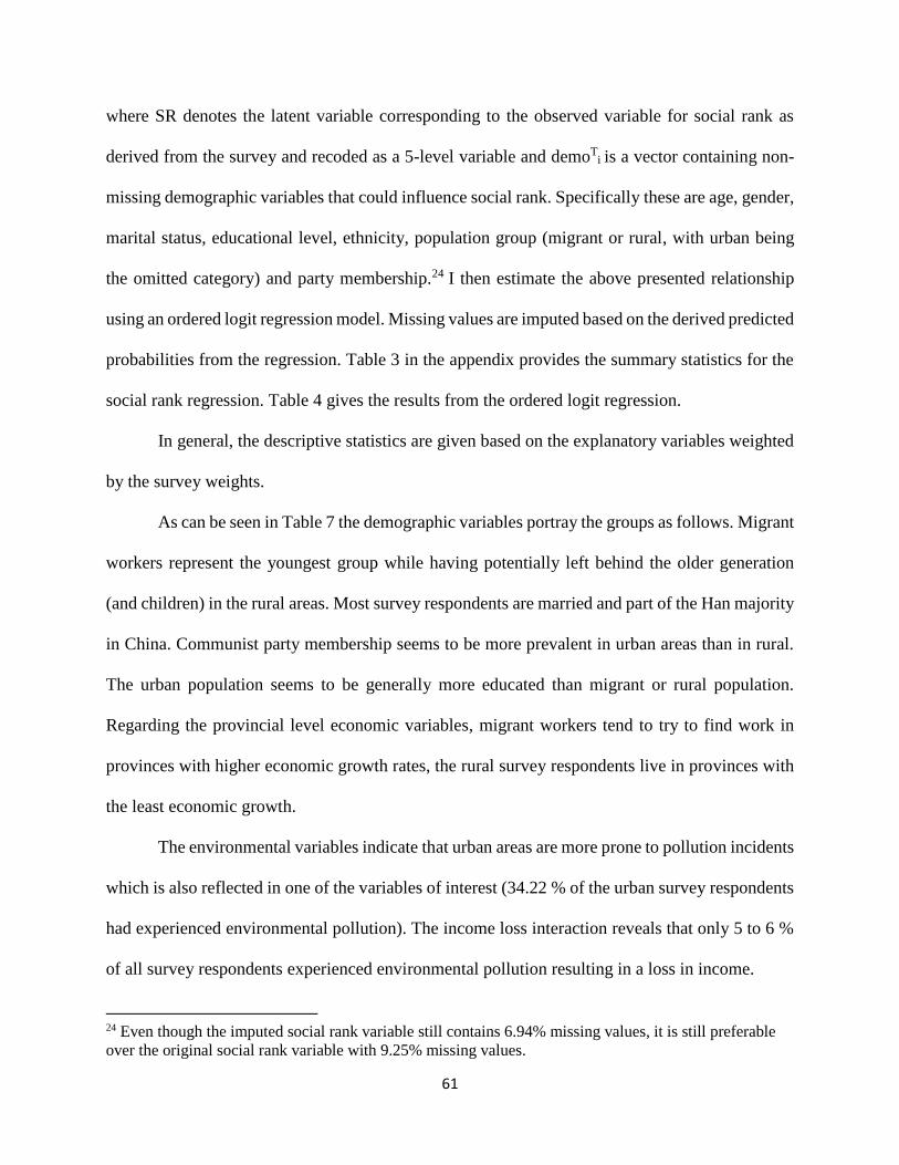
61

where SR denotes the latent variable corresponding to the observed variable for social rank as

derived from the survey and recoded as a 5-level variable and demoTi is a vector containing non-

missing demographic variables that could influence social rank. Specifically these are age, gender,

marital status, educational level, ethnicity, population group (migrant or rural, with urban being

the omitted category) and party membership.24 I then estimate the above presented relationship

using an ordered logit regression model. Missing values are imputed based on the derived predicted

probabilities from the regression. Table 3 in the appendix provides the summary statistics for the

social rank regression. Table 4 gives the results from the ordered logit regression.

In general, the descriptive statistics are given based on the explanatory variables weighted

by the survey weights.

As can be seen in Table 7 the demographic variables portray the groups as follows. Migrant

workers represent the youngest group while having potentially left behind the older generation

(and children) in the rural areas. Most survey respondents are married and part of the Han majority

in China. Communist party membership seems to be more prevalent in urban areas than in rural.

The urban population seems to be generally more educated than migrant or rural population.

Regarding the provincial level economic variables, migrant workers tend to try to find work in

provinces with higher economic growth rates, the rural survey respondents live in provinces with

the least economic growth.

The environmental variables indicate that urban areas are more prone to pollution incidents

which is also reflected in one of the variables of interest (34.22 % of the urban survey respondents

had experienced environmental pollution). The income loss interaction reveals that only 5 to 6 %

of all survey respondents experienced environmental pollution resulting in a loss in income.

24 Even though the imputed social rank variable still contains 6.94% missing values, it is still preferable

over the original social rank variable with 9.25% missing values.

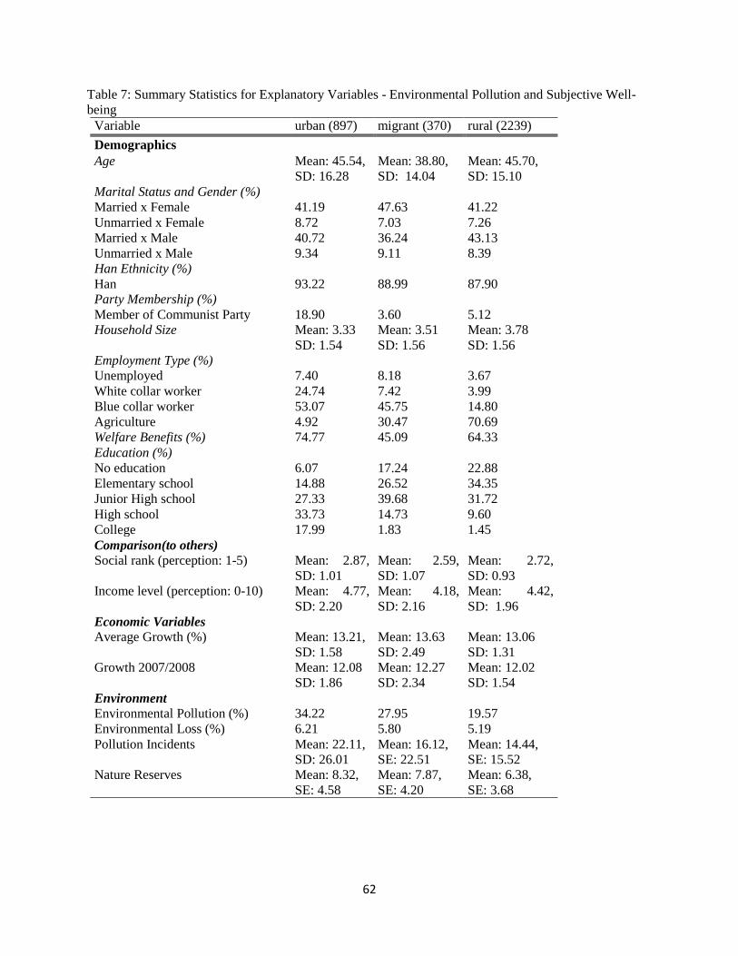
62

Table 7: Summary Statistics for Explanatory Variables - Environmental Pollution and Subjective Well-

being

Variable urban (897) migrant (370) rural (2239)

Demographics

Age Mean: 45.54,

SD: 16.28

Mean: 38.80,

SD: 14.04

Mean: 45.70,

SD: 15.10

Marital Status and Gender (%)

Married x Female 41.19 47.63 41.22

Unmarried x Female 8.72 7.03 7.26

Married x Male 40.72 36.24 43.13

Unmarried x Male 9.34 9.11 8.39

Han Ethnicity (%)

Han

93.22

88.99

87.90

Party Membership (%)

Member of Communist Party

Household Size

Employment Type (%)

18.90

Mean: 3.33

SD: 1.54

3.60

Mean: 3.51

SD: 1.56

5.12

Mean: 3.78

SD: 1.56

Unemployed 7.40 8.18 3.67

White collar worker 24.74 7.42 3.99

Blue collar worker 53.07 45.75 14.80

Agriculture 4.92 30.47 70.69

Welfare Benefits (%) 74.77 45.09 64.33

Education (%)

No education 6.07 17.24 22.88

Elementary school 14.88 26.52 34.35

Junior High school 27.33 39.68 31.72

High school 33.73 14.73 9.60

College 17.99 1.83 1.45

Comparison(to others)

Social rank (perception: 1-5) Mean: 2.87,

SD: 1.01

Mean: 2.59,

SD: 1.07

Mean: 2.72,

SD: 0.93

Income level (perception: 0-10) Mean: 4.77,

SD: 2.20

Mean: 4.18,

SD: 2.16

Mean: 4.42,

SD: 1.96

Economic Variables

Average Growth (%) Mean: 13.21,

SD: 1.58

Mean: 13.63

SD: 2.49

Mean: 13.06

SD: 1.31

Growth 2007/2008 Mean: 12.08

SD: 1.86

Mean: 12.27

SD: 2.34

Mean: 12.02

SD: 1.54

Environment

Environmental Pollution (%) 34.22 27.95 19.57

Environmental Loss (%) 6.21 5.80 5.19

Pollution Incidents Mean: 22.11,

SD: 26.01

Mean: 16.12,

SE: 22.51

Mean: 14.44,

SE: 15.52

Nature Reserves Mean: 8.32,

SE: 4.58

Mean: 7.87,

SE: 4.20

Mean: 6.38,

SE: 3.68

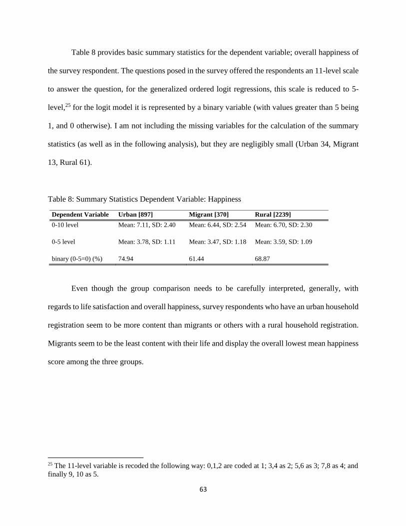
63

Table 8 provides basic summary statistics for the dependent variable; overall happiness of

the survey respondent. The questions posed in the survey offered the respondents an 11-level scale

to answer the question, for the generalized ordered logit regressions, this scale is reduced to 5-

level,25 for the logit model it is represented by a binary variable (with values greater than 5 being

1, and 0 otherwise). I am not including the missing variables for the calculation of the summary

statistics (as well as in the following analysis), but they are negligibly small (Urban 34, Migrant

13, Rural 61).

Table 8: Summary Statistics Dependent Variable: Happiness

Dependent Variable Urban [897] Migrant [370] Rural [2239]

0-10 level Mean: 7.11, SD: 2.40 Mean: 6.44, SD: 2.54 Mean: 6.70, SD: 2.30

0-5 level Mean: 3.78, SD: 1.11 Mean: 3.47, SD: 1.18 Mean: 3.59, SD: 1.09

binary (0-5=0) (%) 74.94 61.44 68.87

Even though the group comparison needs to be carefully interpreted, generally, with

regards to life satisfaction and overall happiness, survey respondents who have an urban household

registration seem to be more content than migrants or others with a rural household registration.

Migrants seem to be the least content with their life and display the overall lowest mean happiness

score among the three groups.

25 The 11-level variable is recoded the following way: 0,1,2 are coded at 1; 3,4 as 2; 5,6 as 3; 7,8 as 4; and

finally 9, 10 as 5.

64

Furthermore, as can be seen

in Figure 4, 29.2 % of the urban

survey respondents would consider

themselves to be in the highest

happiness category, whereas only

20.3% of migrants would answer

the same way. Conversely, a

smaller percentage of the urban

population falls within the lower

happiness categories compared to migrants and rural residents.

3.3. Results

I first estimate the model using the full sample, that is, the pooled sample including the

migrant, rural and urban population groups. Secondly, I estimate it separately for each of the

groups to be able to observe potential differences in the effect of the variables of interest on the

SWB of the survey respondents. In all specifications the standard errors are clustered on county

level.

3.3.1. Logit Model

As the first step I estimate the model as a logit model. The 11-level happiness variable is

coded as a 0/1 variable, with the 0-5 level being 0, and 6-10 level equal to 1, implying the

respondent considers herself to be happy. The results are reported in Table 9 as marginal effects.

Figure 4: Happiness across Population Groups

65

The control variables indicating a missing value as well as some of the education, employment

variables and the household size are presented in Table 4 in Appendix C.

The first column presents the results looking at the effect of basic demographic variables

on the happiness of the survey respondents. The results are consistent with some of the literature

on SWB and China (see for example Jiang et al. 2012). Age has a u-shaped influence, more

education results in higher SWB (aside from just elementary school by itself does not have a

significant influence), marriage has a positive effect. The effect of marriage on SWB is important

for both men and women, even though unmarried women still seem to be more likely to report

being happy than unmarried men (the omitted category). Specific to China it seems to be beneficial

to be a member of the Communist Party.

Based on the first results I include more variables to the regression. Among the two

variables of interest, environmental pollution and the potential to result in a loss in income, only

the loss in income from environmental pollution proves to be significant in the full sample. A loss

in income would have a rather large effect on SWB; having suffered such a loss results in nearly

10 percentage points (depending on the specification) decrease in the probability for the survey

respondent to consider herself happy. However, the significance is strongly diminished when

looking at the combination of environmental pollution and the income loss. Even though the

coefficient remains negative (-0.0547) the p-value is 0.224. The number of pollution incidents

within the province of the survey respondents is also significant in the full specification; however,

the effect is rather small (less than 1 percentage point).

Overall, the provincial economic variables (such as average growth rate) and especially the

personal comparison variables seem to have a constantly significant and large effect on SWB.

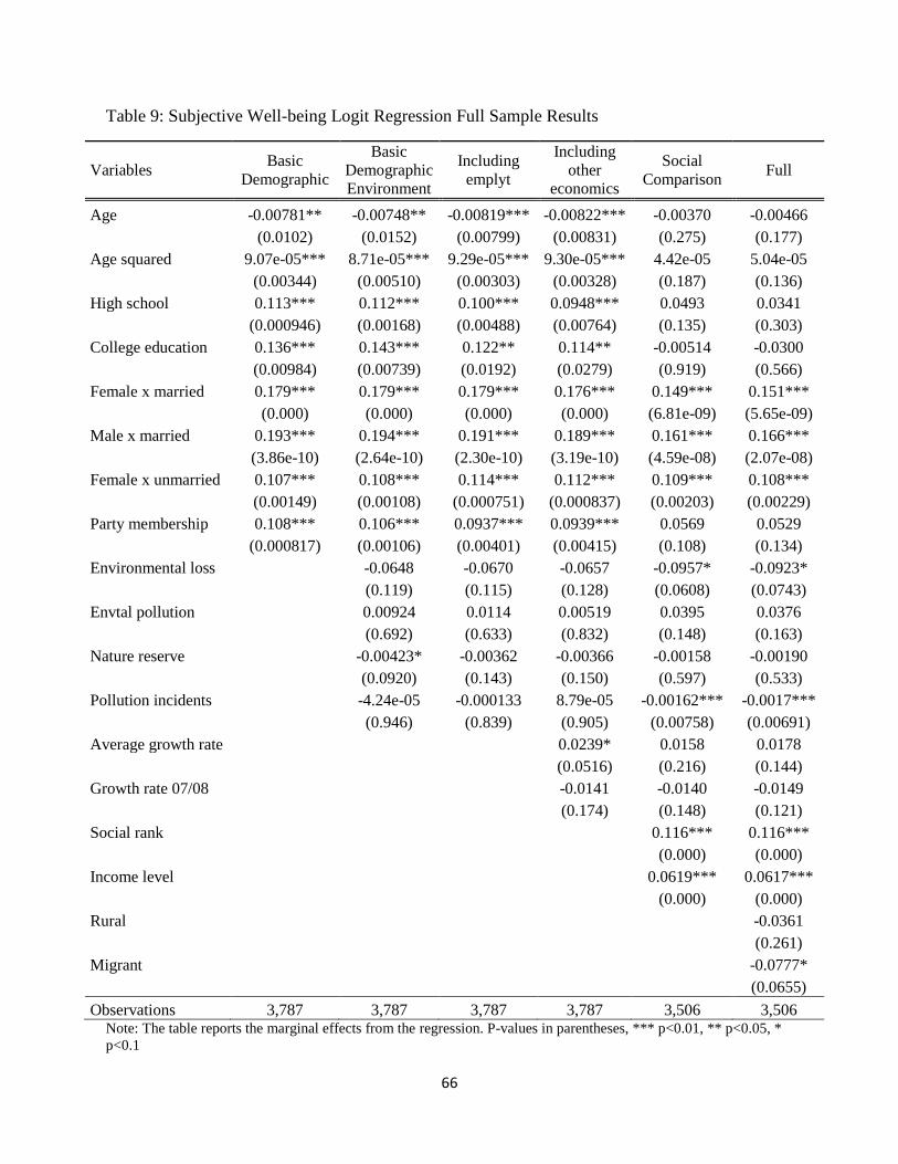
66

Table 9: Subjective Well-being Logit Regression Full Sample Results

Variables Basic

Demographic

Basic

Demographic

Environment

Including

emplyt

Including

other

economics

Social

Comparison Full

Age -0.00781** -0.00748** -0.00819*** -0.00822*** -0.00370 -0.00466

(0.0102) (0.0152) (0.00799) (0.00831) (0.275) (0.177)

Age squared 9.07e-05*** 8.71e-05*** 9.29e-05*** 9.30e-05*** 4.42e-05 5.04e-05

(0.00344) (0.00510) (0.00303) (0.00328) (0.187) (0.136)

High school 0.113*** 0.112*** 0.100*** 0.0948*** 0.0493 0.0341

(0.000946) (0.00168) (0.00488) (0.00764) (0.135) (0.303)

College education 0.136*** 0.143*** 0.122** 0.114** -0.00514 -0.0300

(0.00984) (0.00739) (0.0192) (0.0279) (0.919) (0.566)

Female x married 0.179*** 0.179*** 0.179*** 0.176*** 0.149*** 0.151***

(0.000) (0.000) (0.000) (0.000) (6.81e-09) (5.65e-09)

Male x married 0.193*** 0.194*** 0.191*** 0.189*** 0.161*** 0.166***

(3.86e-10) (2.64e-10) (2.30e-10) (3.19e-10) (4.59e-08) (2.07e-08)

Female x unmarried 0.107*** 0.108*** 0.114*** 0.112*** 0.109*** 0.108***

(0.00149) (0.00108) (0.000751) (0.000837) (0.00203) (0.00229)

Party membership 0.108*** 0.106*** 0.0937*** 0.0939*** 0.0569 0.0529

(0.000817) (0.00106) (0.00401) (0.00415) (0.108) (0.134)

Environmental loss -0.0648 -0.0670 -0.0657 -0.0957* -0.0923*

(0.119) (0.115) (0.128) (0.0608) (0.0743)

Envtal pollution 0.00924 0.0114 0.00519 0.0395 0.0376

(0.692) (0.633) (0.832) (0.148) (0.163)

Nature reserve -0.00423* -0.00362 -0.00366 -0.00158 -0.00190

(0.0920) (0.143) (0.150) (0.597) (0.533)

Pollution incidents -4.24e-05 -0.000133 8.79e-05 -0.00162*** -0.0017***

(0.946) (0.839) (0.905) (0.00758) (0.00691)

Average growth rate 0.0239* 0.0158 0.0178

(0.0516) (0.216) (0.144)

Growth rate 07/08 -0.0141 -0.0140 -0.0149

(0.174) (0.148) (0.121)

Social rank 0.116*** 0.116***

(0.000) (0.000)

Income level 0.0619*** 0.0617***

(0.000) (0.000)

Rural -0.0361

(0.261)

Migrant -0.0777*

(0.0655)

Observations 3,787 3,787 3,787 3,787 3,506 3,506 Note: The table reports the marginal effects from the regression. P-values in parentheses, *** p<0.01, ** p<0.05, *

p<0.1

67

I also include binary variables indicating if the survey respondent has a rural household

registration (but not a migrant) or is part of the rural-to-urban migration subpopulation in the full

model. Being a migrant significantly affects overall SWB of the survey respondent, resulting in a

nearly 8 percentage points’ loss in probability for the survey respondent to consider herself happy.

Having a rural household registration (without being a migrant worker) also negatively affects

SWB, however, it is not significant at any conventional significance level.

3.3.2. Results based on population groups

The results from section 3.3.1 provide a baseline for the separate estimations according to

the three distinct populations. When including indicator variables for rural and migrant, it could

already be seen that individual’s happiness can be affected based on the survey respondent’s

population group. I thus analyze the data using the logit model, now individually for each of the 3

groups. Table 10 reports the results for the logit regression, now divided into the three population

groups. It also includes a column with urban and migrant population combined, as the migrant

workers moved to the cities for work and might perceive environmental pollution from the urban

standpoint. The results for the control variables for the missing values as well as for the

employment variables and the welfare indicator are reported in Table 7 in Appendix C.

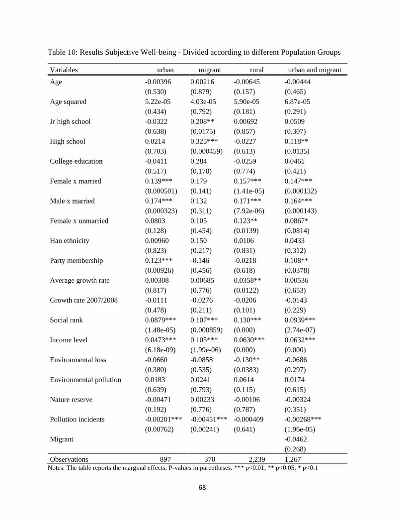
68

Table 10: Results Subjective Well-being - Divided according to different Population Groups

Variables urban migrant rural urban and migrant

Age -0.00396 0.00216 -0.00645 -0.00444

(0.530) (0.879) (0.157) (0.465)

Age squared 5.22e-05 4.03e-05 5.90e-05 6.87e-05

(0.434) (0.792) (0.181) (0.291)

Jr high school -0.0322 0.208** 0.00692 0.0509

(0.638) (0.0175) (0.857) (0.307)

High school 0.0214 0.325*** -0.0227 0.118**

(0.703) (0.000459) (0.613) (0.0135)

College education -0.0411 0.284 -0.0259 0.0461

(0.517) (0.170) (0.774) (0.421)

Female x married 0.139*** 0.179 0.157*** 0.147***

(0.000501) (0.141) (1.41e-05) (0.000132)

Male x married 0.174*** 0.132 0.171*** 0.164***

(0.000323) (0.311) (7.92e-06) (0.000143)

Female x unmarried 0.0803 0.105 0.123** 0.0867*

(0.128) (0.454) (0.0139) (0.0814)

Han ethnicity 0.00960 0.150 0.0106 0.0433

(0.823) (0.217) (0.831) (0.312)

Party membership 0.123*** -0.146 -0.0218 0.108**

(0.00926) (0.456) (0.618) (0.0378)

Average growth rate 0.00308 0.00685 0.0358** 0.00536

(0.817) (0.776) (0.0122) (0.653)

Growth rate 2007/2008 -0.0111 -0.0276 -0.0206 -0.0143

(0.478) (0.211) (0.101) (0.229)

Social rank 0.0879*** 0.107*** 0.130*** 0.0939***

(1.48e-05) (0.000859) (0.000) (2.74e-07)

Income level 0.0473*** 0.105*** 0.0630*** 0.0632***

(6.18e-09) (1.99e-06) (0.000) (0.000)

Environmental loss -0.0660 -0.0858 -0.130** -0.0686

(0.380) (0.535) (0.0383) (0.297)

Environmental pollution 0.0183 0.0241 0.0614 0.0174

(0.639) (0.793) (0.115) (0.615)

Nature reserve -0.00471 0.00233 -0.00106 -0.00324

(0.192) (0.776) (0.787) (0.351)

Pollution incidents -0.00201*** -0.00451*** -0.000409 -0.00268***

(0.00762) (0.00241) (0.641) (1.96e-05)

Migrant -0.0462

(0.268)

Observations 897 370 2,239 1,267 Notes: The table reports the marginal effects. P-values in parentheses. *** p<0.01, ** p<0.05, * p<0.1

69

The subjective comparison variables prove again to be highly significant in all three

subgroups. However, the coefficients do not test statistically significant between the three groups

at any conventional significance level. Being married is still beneficial for SWB and being

unmarried as a man as the omitted category once again seems to be the least satisfying among all

four marriage groups.

A few factors clearly produce surprising results such as being a white collar worker has a

negative influence on happiness for urban residents (compared to being a blue collar worker).

Most importantly, though, having a loss in income resulting from environmental pollution

strongly affects the SWB of rural households whereas environmental pollution itself almost has a

significant positive affect (p-value =0.115). This could indicate that environmental pollution is less

important than the potential economic growth that could stem from it or is accompanied by the

pollution. However, once again, the significance of the environmental shock variables diminishes

when looking at the overall effect (p-value=0.210) with the coefficient staying negative (-0.0684).

It should also be mentioned that the coefficients do not test significantly different between the

three groups. Table 5 and 6 in Appendix C show the results from the second possible specification

of the environmental shock variables as described in the econometric framework.

The number of pollution incidents has a negative impact on the happiness of the migrant

and urban population. That could stem from a general higher number of pollution incidents in

cities. The coefficient for pollution incidents remains negative but insignificant in rural areas.

Given the insignificance and the small absolute value of this coefficient it could also be argued

that the number of pollution incidents (even on provincial level, so not personally experienced) is

a proxy for economic development in the region. This idea might be supported by the fact that the

70

provincial-level economic variables are only significant for the rural subsamples (but there with

the expected signs), indicating the importance of economic development in rural areas.

3.3.3. Generalized Ordered Logit Model and Robustness Check

Lastly, given the ordinal structure of the dependent variables, I am using the generalized

ordered logit model for the full model.26 An alternative could be the ordered logit model, however,

the parallel odds assumption can be rejected (p-value=0.0001). The dependent variable for

happiness now takes 5 values (based on the 11 values from the survey). As can be seen in Table 8

in the appendix, the results for the main variables of interest are consistent to the previous analysis.

Experienced environmental pollution only becomes important if it results in a loss in income and

that also only for the lower level of happiness.

Similarly, the other explanatory variables exhibit the expected sign, once again with the

individually comparative variables (social rank and income level) to be highly significant.

Furthermore, using the recoded 5-level happiness variable as the dependent variable as well,

Table 9 in Appendix C provides the results from a linear (OLS) regression (with standard errors

clustered on county level as well). The first column reports the results from the full sample, the

other four for urban and migrants, and urban, migrant and rural population separately. As can be

seen the results are very similar to those discussed above; i.e. marriage is important for SWB as is

education and the perceived social rank compared to others. With regard to the environmental

variables, the interaction term, loss in income is negative and significant in the full sample.

Environmental pollution itself now is positive and significant (which could indicate economic

26 In this case, the standard errors are not clustered on county level so that the model can be estimated.

71

growth, especially since it is only significant in the migrant and rural subsample). However, once

again the overall term environmental pollution combined with loss, even though negative, is not

significant.

3.3.4. Extension: Natural Disaster

As discussed in the overview of the literature on SWB one set of studies focuses on the

impact of natural disasters on SWB. On May 12, 2008 one of the greatest earthquake in China's

recent history hit Sichuan Province. Given the varying results on SWB and disasters in the

literature, The China Survey provides the opportunity to take a closer look at the relationship

between disasters and SWB. 15.52% of the survey respondents within the full sample of the

analysis were interviewed after May 12, 2008.27 Table 10 in Appendix C provides the results

(marginal effects) from the full logit model, in which I am now including a binary variable

indicating whether the respondent was interviewed before or after the earthquake. As can be seen,

the marginal effects neither change much for the control variables nor for the environmental

variables of interest. The binary variable for the Sichuan earthquake proves to be significant (at

the 10 percent level) and positive, indicating that being interviewed after the earthquake had taken

place increases the likelihood of the survey respondent to consider herself happy. Clearly, the

proportion of respondents being interviewed after the earthquake is comparatively small and China

itself is a large country. Not controlling for proximity to the region affected by the earthquake has

the potential to distort the results. Still, they seem to partially confirm the analysis by Yamamura

(2012) and suggest that such a devastating natural disaster can shift people’s perspectives on life.

27 Stockmann and Landry (2009) use The China Survey and the Sichuan earthquake to look at media

coverage and support for the political system.

72

3.4. Conclusion

By having a strong focus on rural areas this chapter has contributed to the literature on

SWB overall and on China specifically. Rural China has been neglected in many of the

environmental SWB studies on China. However, given that the large percentage of China’s

population still lives in rural areas, it is important to include that part of the population as well.

Furthermore, with this analysis I try to discern the effect of directly experienced environmental

pollution and the potential loss in income arising from environmental pollution.

Overall, the above analysis confirms the influence of various explanatory variables on

happiness in China. In the full sample, age has a u-shaped effect on SWB, being married and

having a higher level of education seems to be important. Specific to China is also the significance

of party membership in the full sample (until inclusion of further variables) and for the urban

subpopulation, as has already been established for example by Jiang et al. (2012), among others.

With regards to environmental conditions the results show that personally experienced

environmental pollution could have an impact on SWB in China overall. However, the effect

seems to be only present in the small interaction term indicating a loss in income for the person

concerned. Furthermore, when looking at the subpopulations, only the subsample for the rural

population exhibits a negative significant effect. It should be kept in mind though that the survey

used for the analysis oversamples the rural areas and hence, both, the sample size for migrants and

the urban population, are much smaller. Still, this result seems to indicate that when environmental

pollution does not result in a loss in income, it does not necessarily effect the SWB of the rural

population.

73

Other, environmental indicators prove to be less important for SWB as compared to

previous studies on China (Smyth et al., 2008; Smyth et al., 2011). The indicators available for

this chapter are, however, rather coarse as they are based mostly on provincial level. More detailed

indicators are mainly only available for urban areas in China. Still the number of pollution

incidents per province seems to have a negative and significant impact on the SWB in the urban

area and in one of the specifications for the overall sample.

Given the increasing number of pollution related protests in China, this result may seem

surprising. Still, most of the protests that are actually made known happen in urban areas. The

number of violent protest in rural areas is considered to be much higher than is generally assumed.

In context with this analysis, these protests can be seen as sign of increasing dissatisfaction with

environmental conditions, especially, when – as could be the case in rural areas – the income of

the survey respondent directly depends on environmental conditions. Additionally, economic

growth as measured by the average growth rate seems to be more important for SWB in rural areas.

Hence, polluting industries might be tolerated as they provide a means for higher income

opportunity. However, as soon as their pollution results in a loss in income, they clearly affect

SWB. This result is of importance when considering, in general, awareness of environmental

pollution and the willingness to improve environmental conditions.

Future research should focus on the rural population and look into more detail on

environmental factors influencing SWB in rural areas similar to the indicators that are available

for urban China such as pollution levels themselves.

74

References

“The China Survey” College of Liberal Arts at Texas A&M University in collaboration with the

Research Center for Contemporary China (RCCC) at Peking University (more

information available under: http://thechinasurvey.tamu.edu/html/home.html)

"Chinese Statistical Abstract "Beijing Press,downloaded from China Data Online.

Akay, Alpaslan, Bargain, Olivier, & Zimmermann, Klaus F. (2012). Relative concerns of rural-to-

urban migrants in China. Journal of Economic Behavior & Organization, 81, 421-441.

Ambec, Stefan & Paul Lanoie. (2008). Does it pay to be green? A systematic overview. Academy

of Management Perspectives, 22 (4), 45-62.

Ambec, Stefan, Cohen, Mark A., Elgie, Stewart, & Lanoie, Paul. (2013). The Porter Hypothesis at

20: Can environmental regulation enhance innovation and competitiveness. Review of

Enviromental Economics and Policy, 7(1), 2-22.

Ambrey, Christopher L., & Fleming, Christopher M. (2011). Valuing scenic amenity using life

satisfaction data. Ecological Economics, 72, 106-115.

Anton, Wilma Rose Q., Deltas, George & Khanna, Madhu (2004). Incentives for environmental

self-regulation and implications for environmental performances. Journal of

Environmental Economics and Management, 48, 632-654.

Appleton, Simon, & Song, Lina. (2008). Life Satisfaction in Urban China: Components and

Determinants. World Development, 36(11), 2325-2340.

Arimura, Toshi H., Darnall, Nicole & Katayama, Hajime. (2011). Is ISO 14001 a gateway to more

advanced voluntary action? The case of green supply chain management, Journal of

Environmental Economics and Management, 61, 170-182.

Arimura, Toshi H., Hibiki, Akira & Katayama, Hajime. (2008). Is a voluntary approach an

effective environmental policy instrument? A case for environmental management systems.

Journal of Environmental Economics and Management, 55, 281-295.

Asadullah, M. Niaz, & Chaudhury, Nazmul. (2011). Poisoning the mind: Arsenic contamination

of drinking water wells and children's educational achievement in rural Bangladesh.

Economics of Education Review, 30, 873-888.

Barbose, Galen, Wiser, Ryan, Phadke, Amol & Goldman, Charles. (2008). Managing carbon

regulatory risk in utility resource planning: Current practices in the Western United States.

Energy Policy, 36, 3300-3311.

Barla, Philippe. (2007). ISO 14001 Certification and environmental performance in Quebec's Pulp

and Paper industry. Journal of Environmental Economics and Management, 53, 291-306.

75

Becchetti, Leonardo, & Castriota, Stefano. (2010). The effects of a calamity on income and

wellbeing of poor microfinance borrowers: The case of the 2004 Tsunami shock. Journal

of Development Studies, 46(2), 211-233.

Becchetti, Leonardo, Castriota, Stefano, & Bedoya, David Andrés Londoño. (2007). Climate,

Happiness and the Kyoto protocol: someone does not like it hot. CEIS Working Paper.

University of Rome Tor Vegata.

Becchetti, Leonardo. (2010). The money-happiness relationship in transition countries: Evidence

from Albania. Transition Studies Review, 17, 39-62.

Berger, Eva M. (2010). The Chernobyl disaster, concern about the environment, and life

satisfaction. KYKLOS, 63(1), 1-8.

Bird, Lori, Chapman, Caroline, Logan, Jeff, Sumner, Jenny & Short, Walter. (2011). Evaluating

renewable portfolio standards and carbon cap scenarios in the U.S. electric sector. Energy

Policy, 39, 2573-2585.

Bookwalter, Jeffrey T. , & Dalenberg, Douglas. (2004). Well-being and household factors in South

Africa. Social Indicators Research, 65(3), 333-353.

Bowen, William M., Park, Sunjoo, & Elvery, Joel A. (2013). Empirical estimates of the influence

of renewable portfolio standards on the green economies of states. Economic Development

Quarterly, online. doi: 10.1177/0891242413491316.

Brereton, Finbarr, Clinch, J. Peter, & Ferreira, Susana. (2008). Happiness, geography and the

environment. Ecological Economics, 65, 386-396.

Brockmann, Hilke, Delhey, Jan, Welzel, Christian, & Yuan, Hao. (2009). The China Puzzle:

Falling Happiness in a Rising Economy. Journal of Happiness Studies,10 (4) , 387-405.

Calvo, Rocío, Arcaya, Mariana, Baum, Christopher F., Lowe, Sarah R. & Waters, Mary C.

(2014). Happily ever after? Pre- and – post disaster determinants of happiness among

survivors of hurricane Katrina. Journal of Happiness Studies. Published online DOI

10.1007/s10902-014-9516-5.

Capon, Noel, Farley, John U., & Hoenig, Scott. (1990). Determinants of financial performance: A

meta-analysis. Management Science, 36(10), 1143-1159.

Cappers, Peter & Goldman, Charles. (2010). Financial impact of energy efficiency under a federal

combined efficiency and renewable electricity standard: Case study of a Kansas “super-

utility”. Energy Policy, 38, 3998-4010.

Carley, Sanya, & Brown, Tyler R. (2012). Innovative US energy policy: a review of states' policy

experiences. WIREs Energy and Environment, 2 (5), 488-506.

76

Carley, Sanya, & Miller, Chris J. (2012). Regulatory Stringency and Policy Drivers: A

Reassessment of Renewable Portfolio Standards. The Policy Studies Journal, 40(4), 730-

756.

Carley, Sanya. (2009). State renewable energy electricity policies: An empirical evaluation of

effectiveness. Energy Policy, 37, 3071-3081.

Carley, Sanya. (2011). The era of state energy policy innovation: A review of policy instruments.

Review of Policy Research, 28(3), 265-294.

Carley, Sanya. (2012). A clean energy standard: Experience from the states. Review of Policy

Research, 29 (2), 301-307.

Carroll, Nick, Frijters, Paul, & Shields, Michael A. (2009). Quantifying the costs of drought: New

evidence from life satisfaction data. Journal of Population Economics, 22(2), 445-461.

Chandler, Jess. (2009). Trendy solutions: Why do states adopt Sustainable Energy Portfolio

Standards. Energy Policy, 37, 3274-3281.

Chen, Cliff, Wiser, Ryan, Mills, Andrew, & Bolinger, Mark. (2009). Weighing the costs and

benefits of state renewables portfolio standards in the United States: A comparative

analysis of state-level policy impact projections. Renewable and Sustainable Energy

Reviews, 13, 552-566.

Chen, Juan. (2013). Perceived discrimination and Subjective Well-being among rural-to-urban

migrants in China. Journal of Sociology & Social Welfare, XL(1), 131-156.

Chen, Juan, Chen, Shuo & Landry, Pierre F. (2013). Migration, environmental hazards, and

health outcomes in China. Social Science & Medicine 80, 85-95.

Chen, Zhenghui, & Davey, Gareth. (2008). Happiness and Subjective Wellbeing in Mainland

China. Journal of Happiness Studies, 9, 589-600.

Chen, Zhenghui, & Davey, Gareth. (2009). Subjective Quality of Life in Zhuhai City, South China:

A Public Survey using the International Wellbeing Index. Social Indicators Research, 91,

243-258.

Cheung, Chau-kiu, & Leung, Kwan-kwok. (2004). Forming life satisfaction among different social

groups during the modernization of China. Journal of Happiness Studies, 5, 23-56.

Chu, Rongwei & Hail, Henry Chiu. (2013). Winding road toward the Chinese dream: The U-

shaped relationship between income and life satisfaction among Chinese migrant

workers. Social Indicator Research. Published online DOI 10.1007/s11205-013-0415-7.

77

Clark, Andrew E., Diener, Ed, Georgellis, Yanni, & Lucas, Richard E. (2008). Lags and leads in

life satisfaction: A test of the baseline hypothesis. The Economic Journal, 118, F222-F243.

Clark, Andrew E., Frijters, Paul, & Shields, Michael A. (2008). Relative income, happiness, and

utility: An explanation for the Easterlin Paradox and other puzzles. Journal of Economic

Literature, 46(1), 95-144.

Danzer, Alexander M., & Danzer, Natalia. (2011). The long-term effects of the Chernobyl

Catastrophe on subjective well-being and mental health. Discussion Paper Series.

Forschungsinstitut zur Zukunft der Arbeit, No. 5906.

Dasgupta, Susmita, Hettige, Hemamala & Wheeler, David. (2000). What improves environmental

compliance? Evidence from the Mexican industry. Journal of Environmental Economics

and Management, 39, 39-66.

Dasgupta, Susmita, Laplante, Benoît, Mamingi, Nlandu & Wang, Hua. (2001). Inspections,

pollution prices, and environmental performance: Evidence from China. Ecological

Economics, 36, 487-498.

Davey, Gareth, & Rato, Ricardo. (2012). Subjective Wellbeing in China: A Review. Journal of

Happiness Studies, 13(333-346).

Davey, Gareth, Chen, Zhenghui, & Lau, Anna. (2009). 'Peace in a Thatched Hut - that is Happiness':

Subjective Wellbeing Among Peasants in Rural China. Journal of Happiness Studies, 10,

239-252.

Delmas, Magali A., & Montes-Sancho, Maria J. (2011). U.S. state policies for renewable energy:

Context and effectiveness. Energy Policy, 39, 2273-2288.

Delmas, Magali A., Russo, Michael V., & Montes-Sancho, Maria J. (2007). Deregulation and

environmental differentiation in the electric utility industry. Strategic Management Journal,

28, 189-209.

Di Tella, Rafael, & MacCulloch, Robert. (2006). Some uses of happiness data in economics. The

Journal of Economic Perspectives, 20(1), 25-46.

Dolan, Paul, Peasgood, Tessa, & White, Mathew. (2008). Do we really know what makes us happy?

A review of the economic literature on the factors associated with subjective well-being.

Journal of Economic Psychology, 29(1), 94-122.

Earnhart, Dietrich & Harrington, Donna. (2013). Effect of audits on the extent of compliance with

wastewater discharge limits. working paper.

Earnhart, Dietrich. (2009).The influence of facility characteristics and permit conditions on the

effects of environmental regulatory deterrence. Journal of Regulatory Economics, 36 (3),

247-273.

78

Easterlin, Richard A. (1974). Does economic growth improve the human lot? In P. A. David & M.

W. Reder (Eds.), Nations and Households in Economic Growth: Essays in Honour of

Moses Abramovi. New York: Academic Press Inc. .

Easterlin, Richard A. (2001). Income and Happiness: Towards a Unified Theory. The Economic

Journal, 111, 465-484.

Easterlin, Richard A., Angelescu McVey, Laura, Switek, Malgorzata, Sawangfa, Onnicha, &

Smith Zweig, Jacqueline. (2010). The happiness-income paradox revisited. pnas, 107(52),

22463-22468.

Easterlin, Richard A., Morgan, Robson, Switek, Malgorzata, & Wang, Fei. (2012). China's life

satisfaction, 1990-2010. pnas, 109(25), 9775-9780.

Energy Information Agency (2007), Electric Power Industry Overview 2007,

http://www.eia.gov/cneaf/electricity/page/prim2/toc2.html#traditional [last accessed Nov.

1, 2011].

Energy Information Agency (2011), EIA website on Electricity, http://www.eia.gov/electricity

[last accessed Nov. 1, 2011].

Energy Information Agency (EIA) (2010) , Restructuring of the Electricity Market

http://www.eia.gov/cneaf/electricity/page/restructuring/restructure_elect.html [last

accessed August 8th, 2013].

Evans, Mary E. Liu, Lirong & Stafford, Sarah L. (2011). Do environmental audits improve long-

term compliance? Evidence from manufacturing facilities in Michigan. Journal of

Regulatory Economics, 40, 279-302.

Fabrizio, Kira R. (2012). The effect of regulatory uncertainty on investment: Evidence from

renewable energy generation. Journal of Law, Economics, and Organization. Accessed

online, doi:10.1093/jleo/ews007.

Fedderson, John, Metcalfe, Robert, & Wooden, Mark. (2012). Subjective well-being: Weather

matters; climate doesn't. Melbourne Insitute Working Paper.

Ferreira, Susana, Akay, Alpaslan, Brereton, Finbarr, Cuñado, Juncal, Martinsson, Peter, & Moro,

Mirko. (2012). Life satisfaction and air quality in Europe. Discussion Paper Series.

Forschungsinstitut zur Zukunft der Arbeit, No 6732. Retrieved from

http://hdl.handle.net/10419/62543.

Ferrer-i-Carbonell, Ada, & Gowdy, John M. (2007). Environmental degradation and happiness.

Ecological Economics, 60, 509-516.

Filbeck, Greg, & Gorman, Raymond F. (2004). The relationship between the environmental and

financial performance of public utilities. Environmental and Resource Economics, 29 (2),

137-157.

79

Fischlein, Miriam, & Smith, Timothy M. (2013). Revisiting renewable portfolio standard

effectiveness: Policy design and outcome specification matter. Policy Science, 34. doi: DOI

10.1007/s11077-013-9175-0

FitzRoy, Felix, Franz-Vasdeki, Jennifer, & Papyrakis, Elissaios. (2012). Policy Review: Climate

change policy and Subjective Well-Being. Environmental Policy and Governance, 22, 205-

216.

Fowler, Luke, & Breen, Joseph. (2013). The impact of political factors on states' adoption of

Renewable Portfolio Standards. The Electricity Journal, 26(2), 79-94.

Fremeth, Adam R. (2009). The dynamic relationship between firm capabilities, regulatory policy,

and environmental performance: Renewable energy policy and investment in the U.S.

electric utility sector. (Dissertation, University of Minnesota) Retrieved from ProQuest

Dissertations and Theses (Accession Order No. 3373391).

Fremeth, Adam R., & Shaver, J. Myles. (2013). Strategic rationale for responding to extra-

jurisdictional regulation: Evidence from firm adoption of renewable power in the US.

Strategic Management Journal, 23.

Frey, Bruno S., & Stutzer, Alois. (2002). What can Economists Learn from Happiness Research?

Journal of Economic Literature, 40(2), 402-435.

Frey, Bruno S., Luechinger, Simon, & Stutzer, Alois. (2010). The life satisfaction approach to

environmental valuation. Annual Review of Resource Economics, 2(1), 139-160.

Frijters, Paul, & van Praag, Bernard M. S. (1998). The effects of climate on welfare and well-being

in Russia. Climatic Change, 39, 61-81.

Gao, Song, Meng, Xiangyi & Zhang, Li. (2014). Fiscal decentralization and life satisfaction:

Evidence from urban China. Social Indicator Research, published online DOI

10.1007/s11205-013-0552-z.

Gao, Wenshu, & Smyth, Russell. (2010). What keeps China's migrant workers going?

Expectations and happiness among China's floating population. Department of Economics,

Discussion Paper 14/10.

Gollop, Frank M. & Roberts, Mark J. (1983). Environmental regulations and productivity growth:

The case of fossil-fueld electric power generation. Journal of Political Economy, 91 (4),

654-674.

Graham, Carol, & Pettinato, S. . (2002). Frustrated Achievers: Winners, losers and subjective well-

being in New Market Economies. The Journal of Development Studies, 38(4), 100-140.

80

Grün, Carola, & Grunewald, Nicole. (2010). Subjective well being and the impact of climate

change. Proceedings of the German Development Economics Conference, Hannover.

Retrieved from: http://hdl.handle.net/10419/40008.

Guardiola, Jorge, González-Gómez, Francisco, & Grajales, Ángel Lendechy. (2013). The

influence of water access in subjective well-being: Some evidence in Yucatan, Mexico.

Social Indicators Research, 110 (1), 207-218.

Guillen-Royo, Monica. (2011). Reference group consumption and the subjective wellbeing of the

poor in Peru. Journal of Economic Psychology, 32, 259-272.

Harrington, Donna, Khanna, Madhu & Deltas, George. (2008). Striving to be green: the adoption

of total quality environmental management. Applied Economics, 40, 2995-3007.

Hayo, Bernd. (2007). Happiness in transition: An empirical study on Eastern Europe. Economic

Systems, 31, 204-221.

Helliwell, John F., & Huang, Haifang. (2008). How's your government? International evidence

linking good government and well-being. British Journal of Political Science, 38 (4), 595-

619.

Hertin, Julia, Berkhout, Frans, Wagner, Marcus & Tyteca, Daniel. (2008). Are EMS

environmentally effective? The link between environmental management systems and

environmental performance in European companies. Journal of Environmental Planning

and Management, 51 (2), 259-283.

Innes, Robert & Sam, Abdoul G. (2008). Voluntary pollution reductions and the enforcement of

environmental law: An empirical study of the 33/50 Program. Journal of Law and

Economics, 51, 271-296.

Jaffe, Adam, & Palmer, Karen. (1997). Environmental regulation and innovatoin: A panel data

study. Review of Economics and Statistics, 79(4), 610-619.

Jenner, Steffen, Ovaere, Lotte, & Schindele, Stephan. (2013). The impact of private interest

contributions on RPS adoption. Economics & Politics, 0, 1-13. doi: DOI:

10.1111/ecpo.12018

Jiang, Shiqing, Lu, Ming, & Sato, Hiroshi. (2012). Identity, Inequality, and Happiness: Evidence

from Urban China. World Development, 40(6), 1190-1200.

Johnson, Erik. (2014). The cost of carbon dioxide abatement from state renewable portfolio

standards. Resource and Energy Economics, 36 (2), 332-350.

Johnstone, Nick & Labonne, Julien. (2009). Why do manufacturing facilities introduce

environmental management systems? Improving and/or signaling performance. Ecological

Economics, 68, 719-730.

81

Kahn, Matt. (2012, April 11). Do Renewable Portfolio Standards raise Electricity Prices?

http://greeneconomics.blogspot.com/2012/04/do-renewable-portfolio-standards-

raise.html. [Last accessed April 18, 2014].

Kahn, Shulamit, & Knittel, Christopher R. (2003). The impact of the Clean Air Act Amendments

of 1990 on electric utilities and coal mines: Evidence from the stock market. Recent Work,

Center for the Study of Energy Markets, University of California Energy Institute, UC

Berkeley. Downloaded from: http://escholarship.org/uc/item/3dh7v8bq.

Khanna, Madhu & Damon, Lisa A. (1999). EPA's Voluntary 33/50 Program: Impact on toxic

releases and economic performance of firms. Journal of Environmental Economics and

Management, 37, 1-25.

Khanna, Madhu & Widyawati, Diah. (2011). Fostering regulatory compliance: The role of

environmental self-auditing and audit policies. Review of Law and Economics, 7, 129-163.

Kimball, Miles, Levy, Helen, Ohtake, Fumio, & Tsutsui, Yoshiro. (2006). Unhappiness after

hurricane Katrina. NBER working paper No. 12062.

Knight, John, Song, Lina, & Gunatilaka, Ramani. (2009). Subjective well-being and its

determinants in rural China. China Economic Review, 20, 635-649.

Knight, John, & Gunatilaka, Ramani. (2008). Aspirations, adaptations and subjective well-being

of rural-urban migrants in China. Discussion Paper Series. Department of Economics.

University of Oxford.

Knight, John, & Gunatilaka, Ramani. (2010a). Great Expectations? The Subjective Well-being of

Rural-Urban Migrants in China. World Development, 38(1), 113-124.

Knight, John, & Gunatilaka, Ramani. (2010b). The Rural-Urban Divide in China: Income but not

Happiness? Journal of Development Studies, 46(3), 506-534.

Kountouris, Yiannis, & Remoundou, Kyriaki. (2011). Valuing the welfare cost of forest fires: A

life satisfaction approach. KYKLOS, 64(4), 556-578.

Kroesen, Maarten, Molin, Eric J. E. , Miedema, Henk M. E. , Vos, Henk, Janssen, Sabine A., &

Van Wee, Bert. (2010). Estimation of the effects of aircraft noise on residential satisfaction.

Transportation Research Part D 15, 144-153.

Kung, Harold H. (2012). Impact of deployment of renewable portfolio standard on the electricity

price in the State of Illinois and implications on policies. Energy Policy, 44, 425-430.

Kydes, Andy S. (2007). Impacts of renewable portfolio generation standard on US energy markets.

Energy Policy, 35, 809-814.

82

Lamontagne, Laura Marie. (2013). Essays in energy economics: An inquiry into renewable

portfolio standards. (Dissertation, Clemson University). Retrieved from ProQuest

Dissertations and Theses (Accession Order No. 3592496).

Landry, Pierre F. and Stockmann, Daniela. (2009). Crisis management in an authoritarian regime:

Media effects during the Sichuan Earthquake (August 28, 2009). Available at

SSRN: http://ssrn.com/abstract=1463796 or http://dx.doi.org/10.2139/ssrn.1463796.

Levinson, Arik. (2012). Valuing public goods using happiness data: The case of air quality.

Journal of Public Economics, 96, 869-880.

Linn, Joshua. (2010). The effect of cap-and-trade programs on firms' profits: Evidence from the

Nitrogen Oxides Budget Trading Program. Journal of Environmental Economics and

Management, 59, 1-14.

Linssen, Rik, van Kempen, Luuk, & Kraaykamp, Gerbert. (2011). Subjective well-being in rural

India: The curse of conspicuous consumption. Social Indicators Research, 101, 57-72.

Liu, Huijun, Li, Shuzhuo, Xiao, Qunying and Feldman, M. W. (2013). Social support and

psychological well-being under social change in urban and rural China. Social Indicators

Research, published online DOI 10.1007/s11205-013-0534-1.

Luechinger, Simon, & Raschky, Paul A. (2009). Valuing flood disasters using the life

satisfaction approach. Journal of Public Economics, 93, 620-633.

Luechinger, Simon. (2009). Valuing air quality using the life satisfaction approach. Economic

Journal, 119(536), 482-515.

Luechinger, Simon. (2010). Life satisfaction and transboundary air pollution. Economic Letters,

107, 4-6.

MacKerron, George, & Mourato, Susana. (2009). Life satisfaction and air quality in London.

Ecological Economics, 68, 1441-1453.

Maddison, David, & Rehdanz, Katrin. (2011). The impact of climate on life satisfaction.

Ecological Economics, 70, 2437-2445.

Magat, Wesley A. & Viscusi, W. Kip. (1990). Effectiveness of the EPA's regulatory enforcement:

The case of industrial effluent standards. Journal of Law and Economics, 33 (2), 331-360.

Matisoff, Daniel C. (2008). The adoption of state climate change policies and renewable portfolio

standards: Regional diffusion or internal determinants? Review of Policy Research, 25(6),

527-546.

Meng, Yuxi. (2013). Renewable Portfolio Standard and State-Level Renewables Innovation in the

United States. Conference paper at the 32nd USAEE/IAEE North American Conference.

Menz, Fredric C., & Vachon, Stephan. (2006). The effectiveness of different policy regimes for

promoting wind power: Experiences from the states. Energy Policy, 34, 1786-1796.

83

Menz, Tobias. (2011). Do people habituate to air pollution? Evidence from international life

satisfaction data. Ecological Economics, 71, 211-219.

Morey, Mathew J., & Kirsch, Laurence D. (2013). Retail rate impacts of state and federal electric

utility policies. The Electricity Journal, 26(3), 35-49.

Nielsen, Ingrid, Smyth, Russell, & Zhai, Qingguo. (2010). Subjective well-being of China's off-

farm migrants. Journal of Happiness Studies, 11, 315-333.

North Carolina Solar Center. 2010. Database of State Incentives for Renewable Energy (DSIRE).

Available at http://www.dsireusa.org. Last accessed: November 25th, 2013.

Nwaeze, Emeka T. (2000). Deregulation of the electric power industry: The earnings, risk, and

return effects. Journal of Regulatory Economics, 17(1), 49-67.

Palmer, Karen & Burtraw, Dallas. (2005). Cost-effectiveness of renewable electricity policies.

Energy Economics, 27, 873-894.

Palmer, Karen, Oates, Wallace E., & Portney, Paul R. (1995). Tightening environmental standards:

The benefit-cost or the no-cost paradigm? Journal of Economic Perspectives, 9(4), 119-

132.

Porter, Michael E. (1991). Green Competitiveness. Scientific American, 264(4), 168.

Porter, Michael E., & van der Linde, Claas. (1995). Toward a new conception of the environment-

competitiveness relationship. Journal of Economic Perspectives, 9(4), 97-118.

Potoski, Matthew & Prakash, Aseem. (2005). Covenants with weak swords: ISO 14001 and

facilities’ environmental performance. Journal of Policy Analysis and Management, 24 (4),

745-769.

Prasad, Monica, & Munch, Steven. (2012). State-level renewable electricity policies and

reductions in carbon emissions. Energy Policy, 45, 237-242.

Rabe, Barry G. (2008). States on steroids: The intergovernmental odyssey of American climate

policy. Review of Policy Research, 25 (2), 105-128.

Rassier, Dylan G. & Dietrich Earnhart. (2010). The effect of clean water regulation on profitability:

Testing the Porter Hypothesis. Land Economics, 86 (2), 329-344.

Rato, Ricardo, & Davey, Gareth. (2012). Quality of Life in Macau, China. Social Indicators

Research, 105, 93-108.

Rehdanz, Katrin, & Maddison, David. (2005). Climate and Happiness. Ecological Economics

(52), 111-125.

Reynaud, Arnaud, & Thomas, Alban. (2012). Firm's profitability and regulation in water and

network industries: An empirical analysis. Utilities Policy, xxx, 1-11.

84

Sam, Abdoul G., Khanna, Madhu & Innes, Robert. (2009). Voluntary pollution reduction programs,

environmental management, and environmental performance: An empirical study. Land

Economics, 85 (4), 692-711.

Sanyal, Paroma. (2007). The effect of deregulation on environmental research by electric utilities.

Journal of Regulatory Economics, 31, 335-353.

Shimshack, Jay P. & Ward, Michael B. (2005). Regulator reputation, enforcement, and

environmental compliance”, Journal of Environmental Economics and Management, 50

519-540.

Shimshak, Jay P. & Ward, Michael B. (2008). Enforcement and over-compliance. Journal of

Environmental Economics and Management, 55 (1), 90-105.

Shrimali, Gireesh & Kniefel, Joshua. (2011). Are government policies effective in promoting

deployment of renewable electricity resources?, Energy Policy, 39, 4726-4741.

Shrimali, Gireesh, Jenner, Steffen, Groba, Felix, Chan, Gabriel, & Indvik, Joe. (2012). Have state

renewable portfolio standards really worked? Synthesizin past policy assessments to build

an integrated econometric analysis of RPS effectiveness in the USA. USAEE Working

Paper No. 12-099; DIW Berlin Discussion Paper No. 1258. Available at SSRN:

http://ssrn.com/abstract=2166815 or http://dx.doi.org/10.2139/ssrn.2166815

Smyth, Russell, Mishra, Vinod, & Qian, Xiaolei. (2008). The Environment and Well-Being in

Urban China. Ecological Economics, 68, 547-555.

Smyth, Russell, Nielsen, Ingrid, Zhai, Qingguo, Liu, Tiemin, Liu, Yin, Tang, Chunyong, Wang,

Zhihong, Wang, Zuxiang & Zhang, Juyong. (2011). A study of the impact of

environmental surroundings on personal well-being in urban China using a multi-item

well-being indicator. Population and Environment, 32, 353-375.

Stafford, Sarah L. (2002). The Effect of punishment on firm compliance with hazardous waste

regulations. Journal of Environmental Economics and Management, 44, 290-308.

Stevenson, Betsey, & Wolfers, Justin. (2009). The paradox of declining female happiness

American Economic Journal: Economic Policy, 1(2), 190-225.

Stockmayer, Gabriella, Finch, Vanessa, Komor, Paul, & Mignogna, Rich. (2012). Limiting the

costs of renewable portfolio standards: A review and critique of current methods. Energy

Policy, 42, 155-163.

Stutzer, Alois, & Frey, Bruno S. (2012). Recent development in the economics of happiness: A

selective overview. IZA Discussion Paper No. 7078. Available at SSRN:

http://ssrn.com/abstract=2192854.

85

Sueyoshi, Toshiyuki, & Goto, Mika. (2009). Can environmental investment and expenditure

enhance financial performance of US electric utility firms under the clean air act

amendment of 1990? Energy Policy, 37, 4819-4826.

Sullivan, Patrick, Logan, Jeffrey, Bird, Lori, & Short, Walter. (2009). Comparative analysis of

three proposed federal renwable electricity standards Technical Report (pp. 30): National

Renewable Energy Laboratory.

Telle, Kjetil. (2009). The threat of regulatory environmental inspection: impact on plant

performance. Journal of Regulatory Economics, 35, 154-178.

Tsao, C.-C., Campbell, J. E., Chen, Yihsu. (2011). When renewable portfolio standards meet cap-

and trade regulations in the electricity sector: Market interactions, profits implications, and

policy redundancy. Energy Policy, 39, 3966-3974.

Uchida, Toshihiro & Ferraro, Paul J. (2007). Voluntary development of environmental

management systems: motivations and regulatory implications. Journal of Regulatory

Economics, 32, 37-65.

van Praag, Bernard M. S., & Baarsma, Barbara E. (2005). Using happiness surveys to value

intangibles: The case of airport noise. The Economic Journal, 115, 224-246.

von Kleist, Karsten. (2010). Migrant happiness in China. Journal of Chinese Economics and

Business Studies, 8(2), 157-166.

Wei, Max, Patadia, Shana & Kammen, Daniel M. (2010). Putting renewables and energy

efficiency to work: How many jobs can the clean energy industry generate in the US?.

Energy Policy, 38, 919-931.

Welsch, Heinz, & Kühling, Jan. (2009). Using happiness data for environmental valuation: Issues

and applications. Journal of Economic Surveys, 23(2), 385-406.

Welsch, Heinz. (2006). Environment and happiness: Valuation of air pollution using life

satisfaction data. Ecological Economics, 58, 801-813.

Wen, Xin, & Smyth, Russell. (2010). Economic Openness and Subjective Well-being in China.

China & World Economy, 18(2), 22-40.

Wiser, Ryan, & Barbose, Galen. (2008). Renewable Portfolio Standards in the United States - A

status report with data through 2007. Lawrence Berkely National Laboratory.

Wiser, Ryan, Namovicz, Christopher, Gielecki, Mark, & Smith, Robert. (2007). The Experience

with Renewable Portfolio Standards in the United States. The Electricity Journal, 8-20.

86

Yamamura, Eiji. (2012). Natural disasters and their long-term effect on happiness: the case of the

great Hanshin-Awaji earthquake. MPRA Paper.

Yin, Haitao, & Powers, Nicholas. (2010). Do state renewable portfolio standards promote in-state

renewable generation. Energy Policy, 38, 1140-1149.

Zhai, Qing-guo, O'Shea, Bob, Willis, Mike, & Yang, Yu-wen. (2010). Subjective Well-being,

Personality and Environmental Satisfaction in Urban China. Paper presented at the 2010

International Conference on Management Science & Engineering (17th), Melbourne,

Australia.

Zhao, Wei. (2012). Economic inequality, status perceptions, and subjective well-being in China's

transitional economy. Research in Social Stratification and Mobility, 30 (4), 433-450.

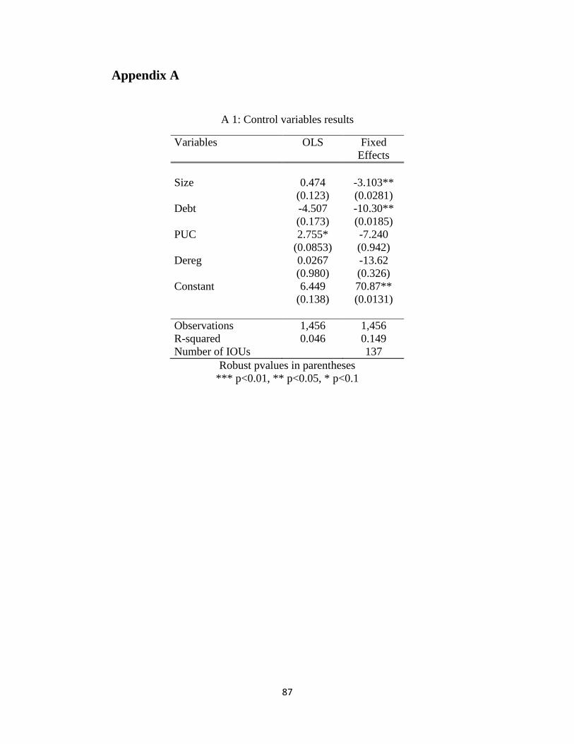
87

Appendix A

A 1: Control variables results

Variables OLS Fixed

Effects

Size 0.474 -3.103**

(0.123) (0.0281)

Debt -4.507 -10.30**

(0.173) (0.0185)

PUC 2.755* -7.240

(0.0853) (0.942)

Dereg 0.0267 -13.62

(0.980) (0.326)

Constant 6.449 70.87**

(0.138) (0.0131)

Observations 1,456 1,456

R-squared 0.046 0.149

Number of IOUs 137

Robust pvalues in parentheses

*** p<0.01, ** p<0.05, * p<0.1

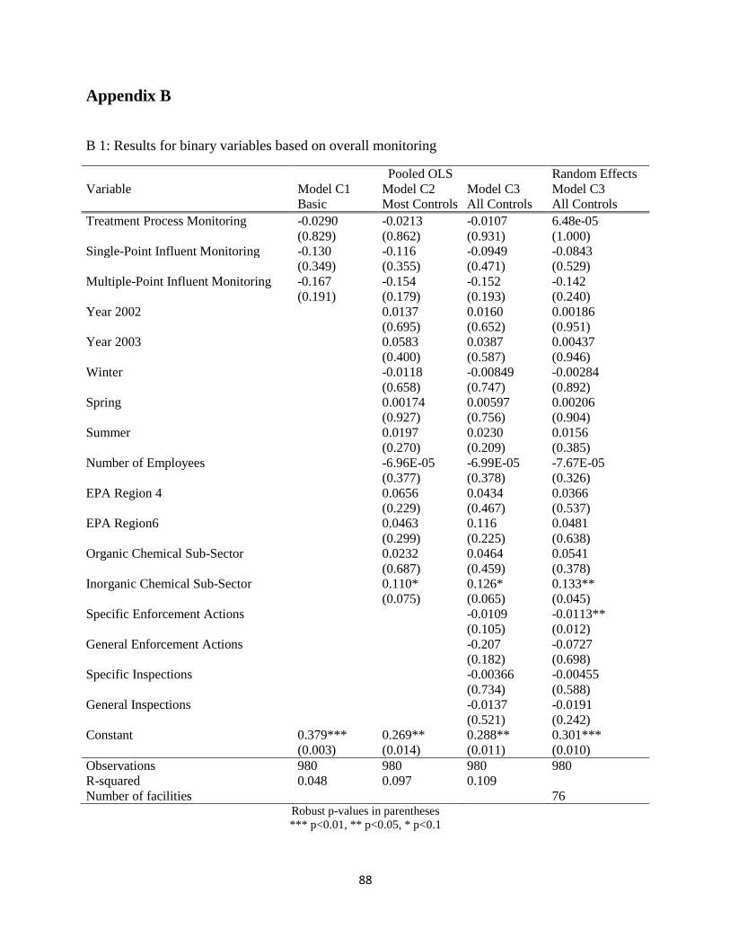
88

Appendix B

B 1: Results for binary variables based on overall monitoring

Pooled OLS Random Effects

Variable Model C1

Basic

Model C2

Most Controls

Model C3

All Controls

Model C3

All Controls

Treatment Process Monitoring -0.0290 -0.0213 -0.0107 6.48e-05

(0.829) (0.862) (0.931) (1.000)

Single-Point Influent Monitoring -0.130 -0.116 -0.0949 -0.0843

(0.349) (0.355) (0.471) (0.529)

Multiple-Point Influent Monitoring -0.167 -0.154 -0.152 -0.142

(0.191) (0.179) (0.193) (0.240)

Year 2002 0.0137 0.0160 0.00186

(0.695) (0.652) (0.951)

Year 2003 0.0583 0.0387 0.00437

(0.400) (0.587) (0.946)

Winter -0.0118 -0.00849 -0.00284

(0.658) (0.747) (0.892)

Spring 0.00174 0.00597 0.00206

(0.927) (0.756) (0.904)

Summer 0.0197 0.0230 0.0156

(0.270) (0.209) (0.385)

Number of Employees -6.96E-05 -6.99E-05 -7.67E-05

(0.377) (0.378) (0.326)

EPA Region 4 0.0656 0.0434 0.0366

(0.229) (0.467) (0.537)

EPA Region6 0.0463 0.116 0.0481

(0.299) (0.225) (0.638)

Organic Chemical Sub-Sector 0.0232 0.0464 0.0541

(0.687) (0.459) (0.378)

Inorganic Chemical Sub-Sector 0.110* 0.126* 0.133**

(0.075) (0.065) (0.045)

Specific Enforcement Actions -0.0109 -0.0113**

(0.105) (0.012)

General Enforcement Actions -0.207 -0.0727

(0.182) (0.698)

Specific Inspections -0.00366 -0.00455

(0.734) (0.588)

General Inspections -0.0137 -0.0191

(0.521) (0.242)

Constant 0.379*** 0.269** 0.288** 0.301***

(0.003) (0.014) (0.011) (0.010)

Observations 980 980 980 980

R-squared 0.048 0.097 0.109

Number of facilities 76 Robust p-values in parentheses

*** p<0.01, ** p<0.05, * p<0.1

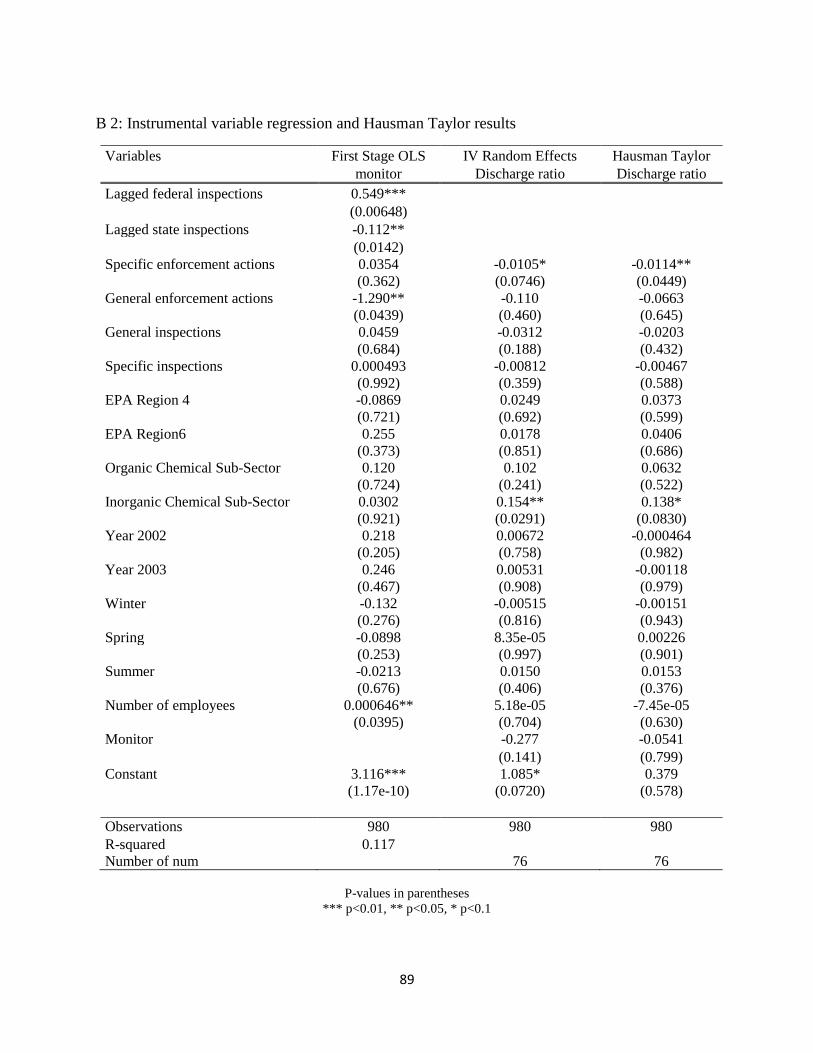
89

B 2: Instrumental variable regression and Hausman Taylor results

Variables First Stage OLS IV Random Effects Hausman Taylor

monitor Discharge ratio Discharge ratio

Lagged federal inspections 0.549*** (0.00648)

Lagged state inspections -0.112** (0.0142) Specific enforcement actions 0.0354 -0.0105* -0.0114**

(0.362) (0.0746) (0.0449)

General enforcement actions -1.290** -0.110 -0.0663

(0.0439) (0.460) (0.645)

General inspections 0.0459 -0.0312 -0.0203

(0.684) (0.188) (0.432)

Specific inspections 0.000493 -0.00812 -0.00467

(0.992) (0.359) (0.588)

EPA Region 4 -0.0869 0.0249 0.0373

(0.721) (0.692) (0.599)

EPA Region6 0.255 0.0178 0.0406

(0.373) (0.851) (0.686)

Organic Chemical Sub-Sector 0.120 0.102 0.0632

(0.724) (0.241) (0.522)

Inorganic Chemical Sub-Sector 0.0302 0.154** 0.138*

(0.921) (0.0291) (0.0830)

Year 2002 0.218 0.00672 -0.000464

(0.205) (0.758) (0.982)

Year 2003 0.246 0.00531 -0.00118

(0.467) (0.908) (0.979)

Winter -0.132 -0.00515 -0.00151

(0.276) (0.816) (0.943)

Spring -0.0898 8.35e-05 0.00226

(0.253) (0.997) (0.901)

Summer -0.0213 0.0150 0.0153

(0.676) (0.406) (0.376)

Number of employees 0.000646** 5.18e-05 -7.45e-05

(0.0395) (0.704) (0.630)

Monitor -0.277 -0.0541

(0.141) (0.799)

Constant 3.116*** 1.085* 0.379

(1.17e-10) (0.0720) (0.578)

Observations 980 980 980

R-squared 0.117 Number of num 76 76

P-values in parentheses

*** p<0.01, ** p<0.05, * p<0.1

90

Appendix C

C 1: Description of Explanatory Variables

Variables Description

Environmental Variables

Environmental pollution = 1 if environmental pollution in last 12 months, 0 otherwise

Environmental loss = 1 if envtal pollution in last 12 months and resulted in loss in income, 0

otherwise (no envtal pollution or envtal pollution but no loss in income)

Nature reserve percentage of area for nature reserves in province where respondent lives

Pollution incidents number of pollution(water pollution, air pollution, solid waste pollution, noise

and vibration pollution) incidents

Demographics

Age continuous variable for age

Female x married = 1 if married female, 0 otherwise

Male x married = 1 if married male, 0 otherwise

Female x unmarried = 1 if unmarried female, 0 otherwise

Male x unmarried = 1 if unmarried male, 0 otherwise

Han ethnicity = 1 if Han ethnicity, 0 otherwise

Party membership = 1 if member of Communist Party, 0 otherwise

No education = 1 if no education, 0 otherwise

Elementary school = 1 if some years of elementary school education, 0 otherwise

Jr high school = 1 if some years of middle school education, 0 otherwise

High school = 1 if some years of high school education, 0 otherwise

College education = 1 if some years of college education, 0 otherwise

Unemployed = 1 if currently no work, 0 otherwise

Agricultural worker = 1 if farmer, animal husbandry, or fishery, 0 otherwise

Blue-collar worker = 1 if laborer / worker, clerk, serviceman, police officer, self-owned business or

owner of private-owned business, 0 otherwise

White-collar worker = 1 if commerce, service trade worker, manager, professional/technical,

employee of government agency, party agency, or social organization, 0

otherwise

Welfare = 1 if respondent has medical insurance, unemployment insurance, pension or

housing subsidy, 0 otherwise

Rural = 1 if rural household registration but not migrant

Migrant = 1 if rural-to-urban migrant

Comparison

Social rank answer to the question: how would you rank your own social status (originally

0-10 scale, rescaled to 5 levels)

Income level answer to the question: compared to the average household income in this

county/city/district, at what level do you feel your household income is situated?

(0-10 scale)

Economic Controls

Average growth rate 5-year average of provincial growth rate

Growth rate 2007/2008 provincial growth rate from 2007-2008

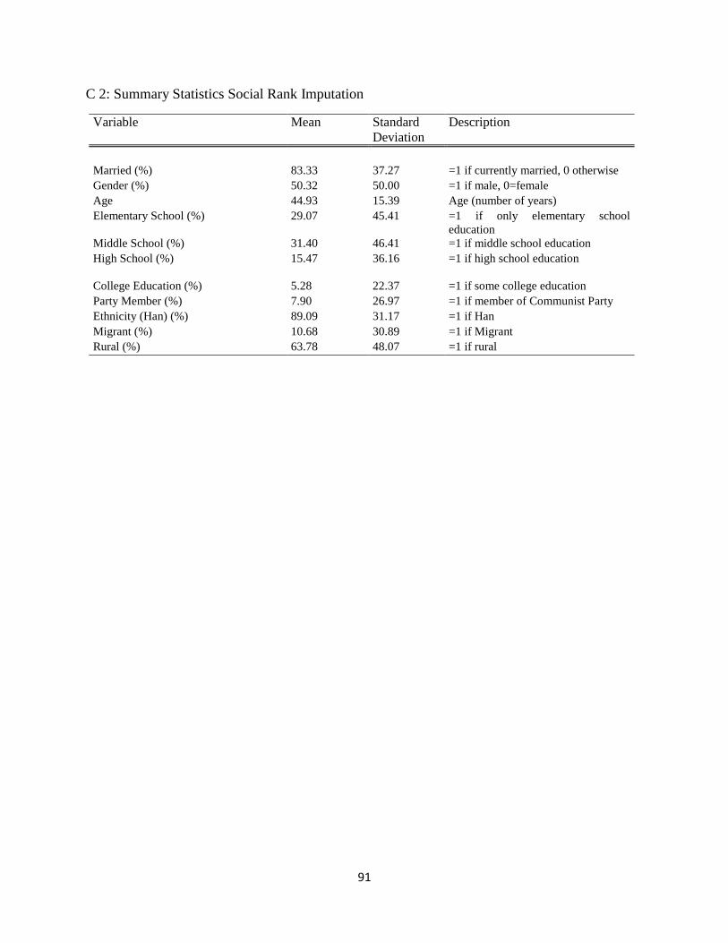
91

C 2: Summary Statistics Social Rank Imputation

Variable Mean Standard

Deviation

Description

Married (%) 83.33 37.27 =1 if currently married, 0 otherwise

Gender (%) 50.32 50.00 =1 if male, 0=female

Age 44.93 15.39 Age (number of years)

Elementary School (%) 29.07 45.41 =1 if only elementary school

education

Middle School (%) 31.40 46.41 =1 if middle school education

High School (%) 15.47

36.16 =1 if high school education

College Education (%) 5.28 22.37 =1 if some college education

Party Member (%) 7.90 26.97 =1 if member of Communist Party

Ethnicity (Han) (%) 89.09 31.17 =1 if Han

Migrant (%) 10.68 30.89 =1 if Migrant

Rural (%) 63.78 48.07 =1 if rural

92

C 3: Ordered Logit Regression Results for Social Rank

Variables Social rank

Age 0.00648*

(0.0520)

Male 0.0483

(0.468)

Married 0.0898

(0.244)

Elementary School 0.251

(0.105)

Middle School 0.326*

(0.0543)

High School 0.460**

(0.0112)

College Education 0.929***

(1.02e-05)

Party member 0.543***

(9.30e-06)

Han 0.125

(0.430)

Migrant -0.230*

(0.0758)

Rural 0.0498

(0.670)

cut1

Constant -0.941**

(0.0110)

cut2

Constant 0.146

(0.680)

cut3

Constant 2.425***

(1.05e-10)

cut4

Constant 4.251***

(0)

Observations 3,539 Robust P-values in parentheses

*** p<0.01, ** p<0.05, * p<0.1

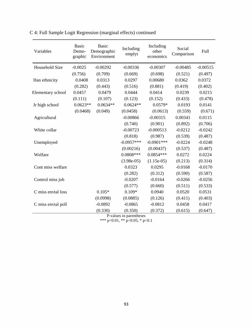
93

C 4: Full Sample Logit Regression (marginal effects) continued

Variables

Basic

Demo-

graphic

Basic

Demographic

Environment

Including

emplyt

Including

other

economics

Social

Comparison Full

Household Size -0.0025 -0.00292 -0.00336 -0.00307 -0.00485 -0.00515

(0.756) (0.709) (0.669) (0.698) (0.521) (0.497)

Han ethnicity 0.0408 0.0313 0.0297 0.00680 0.0362 0.0372

(0.282) (0.443) (0.516) (0.881) (0.419) (0.402)

Elementary school 0.0457 0.0479 0.0444 0.0414 0.0239 0.0215

(0.111) (0.107) (0.123) (0.152) (0.433) (0.478)

Jr high school 0.0623** 0.0634** 0.0624** 0.0579* 0.0193 0.0141

(0.0468) (0.049) (0.0458) (0.0613) (0.559) (0.671)

Agricultural -0.00866 -0.00315 0.00341 0.0115

(0.740) (0.901) (0.892) (0.706)

White collar -0.00723 -0.000513 -0.0212 -0.0242

(0.818) (0.987) (0.539) (0.487)

Unemployed -0.0957*** -0.0901*** -0.0224 -0.0248

(0.00216) (0.00437) (0.537) (0.487)

Welfare 0.0808*** 0.0854*** 0.0272 0.0224

(3.98e-05) (1.15e-05) (0.213) (0.314)

Cont miss welfare 0.0323 0.0295 -0.0168 -0.0170

(0.282) (0.312) (0.590) (0.587)

Control miss job -0.0207 -0.0164 -0.0266 -0.0256

(0.577) (0.660) (0.511) (0.533)

C miss envtal loss 0.105* 0.109* 0.0940 0.0520 0.0531

(0.0998) (0.0885) (0.126) (0.411) (0.403)

C miss envtal poll -0.0892 -0.0865 -0.0812 0.0458 0.0417

(0.330) (0.350) (0.372) (0.615) (0.647) P-values in parentheses

*** p<0.01, ** p<0.05, * p<0.1

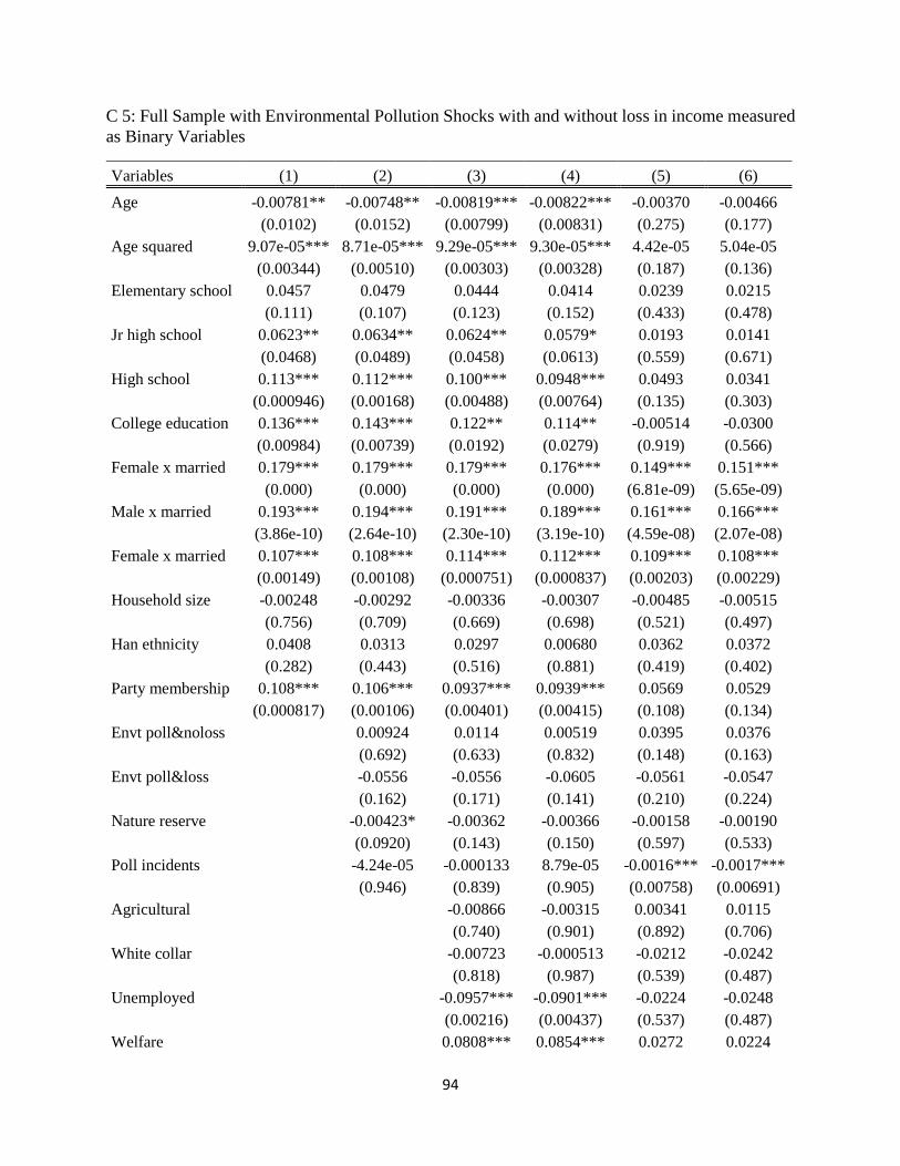
94

C 5: Full Sample with Environmental Pollution Shocks with and without loss in income measured

as Binary Variables

Variables (1) (2) (3) (4) (5) (6)

Age -0.00781** -0.00748** -0.00819*** -0.00822*** -0.00370 -0.00466

(0.0102) (0.0152) (0.00799) (0.00831) (0.275) (0.177)

Age squared 9.07e-05*** 8.71e-05*** 9.29e-05*** 9.30e-05*** 4.42e-05 5.04e-05

(0.00344) (0.00510) (0.00303) (0.00328) (0.187) (0.136)

Elementary school 0.0457 0.0479 0.0444 0.0414 0.0239 0.0215

(0.111) (0.107) (0.123) (0.152) (0.433) (0.478)

Jr high school 0.0623** 0.0634** 0.0624** 0.0579* 0.0193 0.0141

(0.0468) (0.0489) (0.0458) (0.0613) (0.559) (0.671)

High school 0.113*** 0.112*** 0.100*** 0.0948*** 0.0493 0.0341

(0.000946) (0.00168) (0.00488) (0.00764) (0.135) (0.303)

College education 0.136*** 0.143*** 0.122** 0.114** -0.00514 -0.0300

(0.00984) (0.00739) (0.0192) (0.0279) (0.919) (0.566)

Female x married 0.179*** 0.179*** 0.179*** 0.176*** 0.149*** 0.151***

(0.000) (0.000) (0.000) (0.000) (6.81e-09) (5.65e-09)

Male x married 0.193*** 0.194*** 0.191*** 0.189*** 0.161*** 0.166***

(3.86e-10) (2.64e-10) (2.30e-10) (3.19e-10) (4.59e-08) (2.07e-08)

Female x married 0.107*** 0.108*** 0.114*** 0.112*** 0.109*** 0.108***

(0.00149) (0.00108) (0.000751) (0.000837) (0.00203) (0.00229)

Household size -0.00248 -0.00292 -0.00336 -0.00307 -0.00485 -0.00515

(0.756) (0.709) (0.669) (0.698) (0.521) (0.497)

Han ethnicity 0.0408 0.0313 0.0297 0.00680 0.0362 0.0372

(0.282) (0.443) (0.516) (0.881) (0.419) (0.402)

Party membership 0.108*** 0.106*** 0.0937*** 0.0939*** 0.0569 0.0529

(0.000817) (0.00106) (0.00401) (0.00415) (0.108) (0.134)

Envt poll&noloss 0.00924 0.0114 0.00519 0.0395 0.0376

(0.692) (0.633) (0.832) (0.148) (0.163)

Envt poll&loss -0.0556 -0.0556 -0.0605 -0.0561 -0.0547

(0.162) (0.171) (0.141) (0.210) (0.224)

Nature reserve -0.00423* -0.00362 -0.00366 -0.00158 -0.00190

(0.0920) (0.143) (0.150) (0.597) (0.533)

Poll incidents -4.24e-05 -0.000133 8.79e-05 -0.0016*** -0.0017***

(0.946) (0.839) (0.905) (0.00758) (0.00691)

Agricultural -0.00866 -0.00315 0.00341 0.0115

(0.740) (0.901) (0.892) (0.706)

White collar -0.00723 -0.000513 -0.0212 -0.0242

(0.818) (0.987) (0.539) (0.487)

Unemployed -0.0957*** -0.0901*** -0.0224 -0.0248

(0.00216) (0.00437) (0.537) (0.487)

Welfare 0.0808*** 0.0854*** 0.0272 0.0224

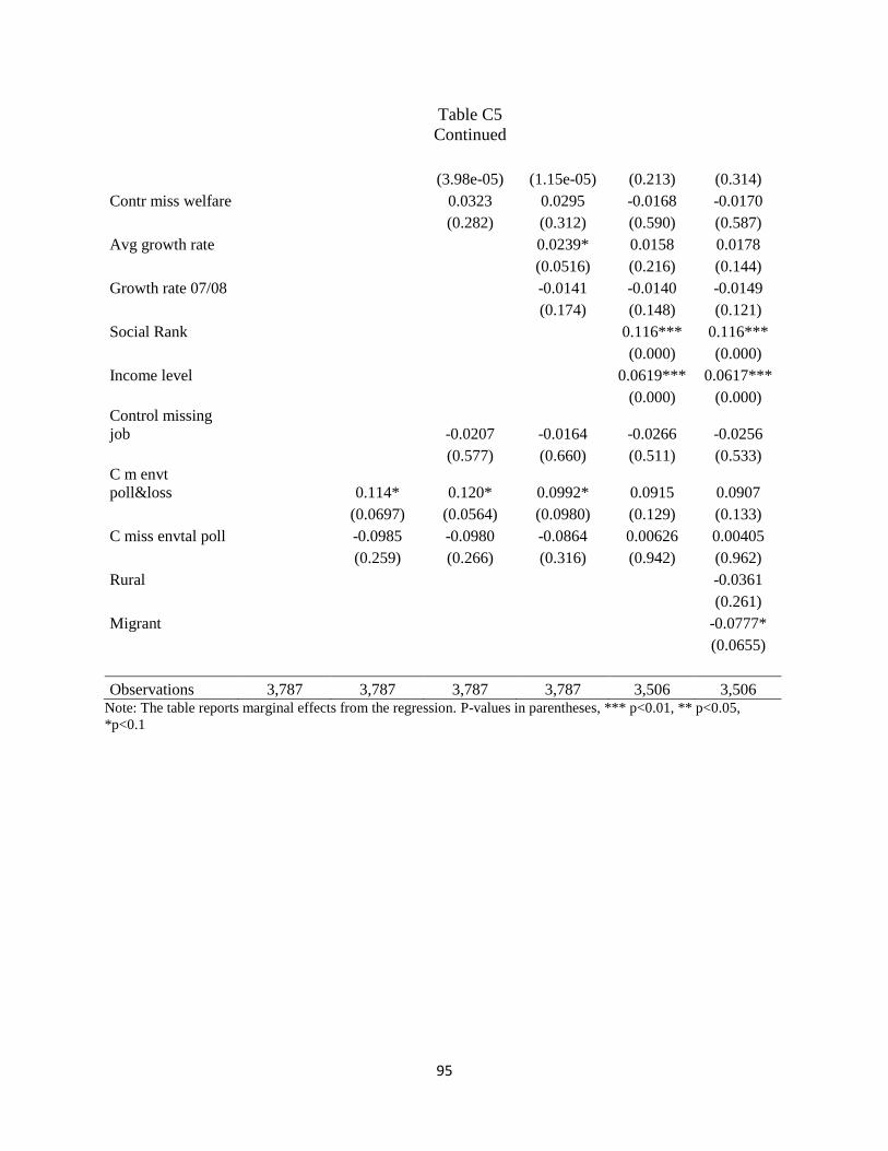
95

Table C5

Continued

(3.98e-05) (1.15e-05) (0.213) (0.314)

Contr miss welfare 0.0323 0.0295 -0.0168 -0.0170

(0.282) (0.312) (0.590) (0.587)

Avg growth rate 0.0239* 0.0158 0.0178

(0.0516) (0.216) (0.144)

Growth rate 07/08 -0.0141 -0.0140 -0.0149

(0.174) (0.148) (0.121)

Social Rank 0.116*** 0.116***

(0.000) (0.000)

Income level 0.0619*** 0.0617***

(0.000) (0.000)

Control missing

job -0.0207 -0.0164 -0.0266 -0.0256

(0.577) (0.660) (0.511) (0.533)

C m envt

poll&loss 0.114* 0.120* 0.0992* 0.0915 0.0907

(0.0697) (0.0564) (0.0980) (0.129) (0.133)

C miss envtal poll -0.0985 -0.0980 -0.0864 0.00626 0.00405

(0.259) (0.266) (0.316) (0.942) (0.962)

Rural -0.0361

(0.261)

Migrant -0.0777*

(0.0655)

Observations 3,787 3,787 3,787 3,787 3,506 3,506 Note: The table reports marginal effects from the regression. P-values in parentheses, *** p<0.01, ** p<0.05,

*p<0.1

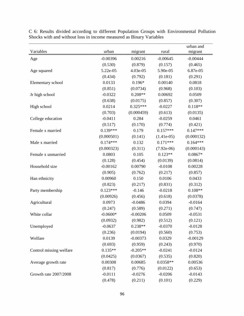
96

C 6: Results divided according to different Population Groups with Environmental Pollution

Shocks with and without loss in income measured as Binary Variables

Variables urban migrant rural

urban and

migrant

Age -0.00396 0.00216 -0.00645 -0.00444

(0.530) (0.879) (0.157) (0.465)

Age squared 5.22e-05 4.03e-05 5.90e-05 6.87e-05

(0.434) (0.792) (0.181) (0.291)

Elementary school 0.0133 0.196* 0.00140 0.0818

(0.851) (0.0734) (0.968) (0.103)

Jr high school -0.0322 0.208** 0.00692 0.0509

(0.638) (0.0175) (0.857) (0.307)

High school 0.0214 0.325*** -0.0227 0.118**

(0.703) (0.000459) (0.613) (0.0135)

College education -0.0411 0.284 -0.0259 0.0461

(0.517) (0.170) (0.774) (0.421)

Female x married 0.139*** 0.179 0.157*** 0.147***

(0.000501) (0.141) (1.41e-05) (0.000132)

Male x married 0.174*** 0.132 0.171*** 0.164***

(0.000323) (0.311) (7.92e-06) (0.000143)

Female x unmarried 0.0803 0.105 0.123** 0.0867*

(0.128) (0.454) (0.0139) (0.0814)

Household size -0.00162 0.00790 -0.0108 0.00228

(0.905) (0.762) (0.217) (0.857)

Han ethnicity 0.00960 0.150 0.0106 0.0433

(0.823) (0.217) (0.831) (0.312)

Party membership 0.123*** -0.146 -0.0218 0.108**

(0.00926) (0.456) (0.618) (0.0378)

Agricultural 0.0973 -0.0486 0.0394 -0.0164

(0.247) (0.589) (0.271) (0.747)

White collar -0.0600* -0.00206 0.0509 -0.0531

(0.0932) (0.982) (0.512) (0.121)

Unemployed -0.0637 0.238** -0.0370 -0.0128

(0.236) (0.0194) (0.560) (0.753)

Welfare 0.0139 -0.00373 0.0329 -0.00129

(0.693) (0.959) (0.243) (0.970)

Control missing welfare 0.135** -0.205** -0.0241 -0.0124

(0.0425) (0.0367) (0.535) (0.820)

Average growth rate 0.00308 0.00685 0.0358** 0.00536

(0.817) (0.776) (0.0122) (0.653)

Growth rate 2007/2008 -0.0111 -0.0276 -0.0206 -0.0143

(0.478) (0.211) (0.101) (0.229)

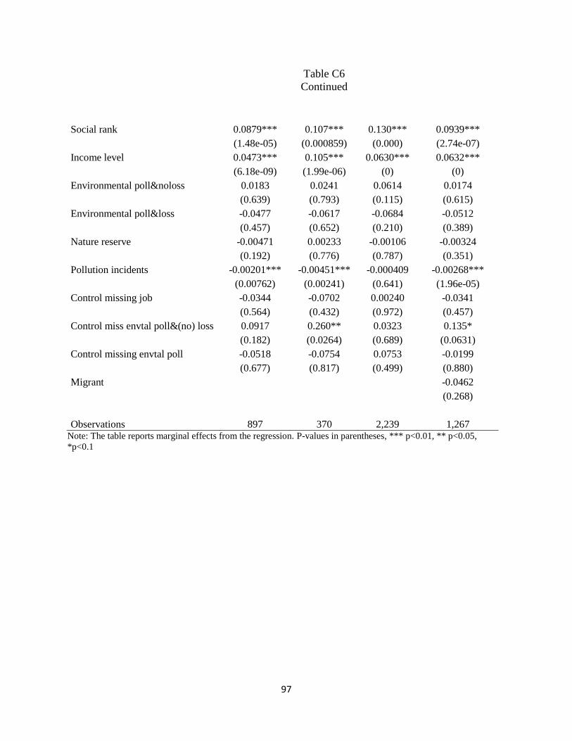
97

Table C6

Continued

Social rank 0.0879*** 0.107*** 0.130*** 0.0939***

(1.48e-05) (0.000859) (0.000) (2.74e-07)

Income level 0.0473*** 0.105*** 0.0630*** 0.0632***

(6.18e-09) (1.99e-06) (0) (0)

Environmental poll&noloss 0.0183 0.0241 0.0614 0.0174

(0.639) (0.793) (0.115) (0.615)

Environmental poll&loss -0.0477 -0.0617 -0.0684 -0.0512

(0.457) (0.652) (0.210) (0.389)

Nature reserve -0.00471 0.00233 -0.00106 -0.00324

(0.192) (0.776) (0.787) (0.351)

Pollution incidents -0.00201*** -0.00451*** -0.000409 -0.00268***

(0.00762) (0.00241) (0.641) (1.96e-05)

Control missing job -0.0344 -0.0702 0.00240 -0.0341

(0.564) (0.432) (0.972) (0.457)

Control miss envtal poll&(no) loss 0.0917 0.260** 0.0323 0.135*

(0.182) (0.0264) (0.689) (0.0631)

Control missing envtal poll -0.0518 -0.0754 0.0753 -0.0199

(0.677) (0.817) (0.499) (0.880)

Migrant -0.0462

(0.268)

Observations 897 370 2,239 1,267 Note: The table reports marginal effects from the regression. P-values in parentheses, *** p<0.01, ** p<0.05,

*p<0.1

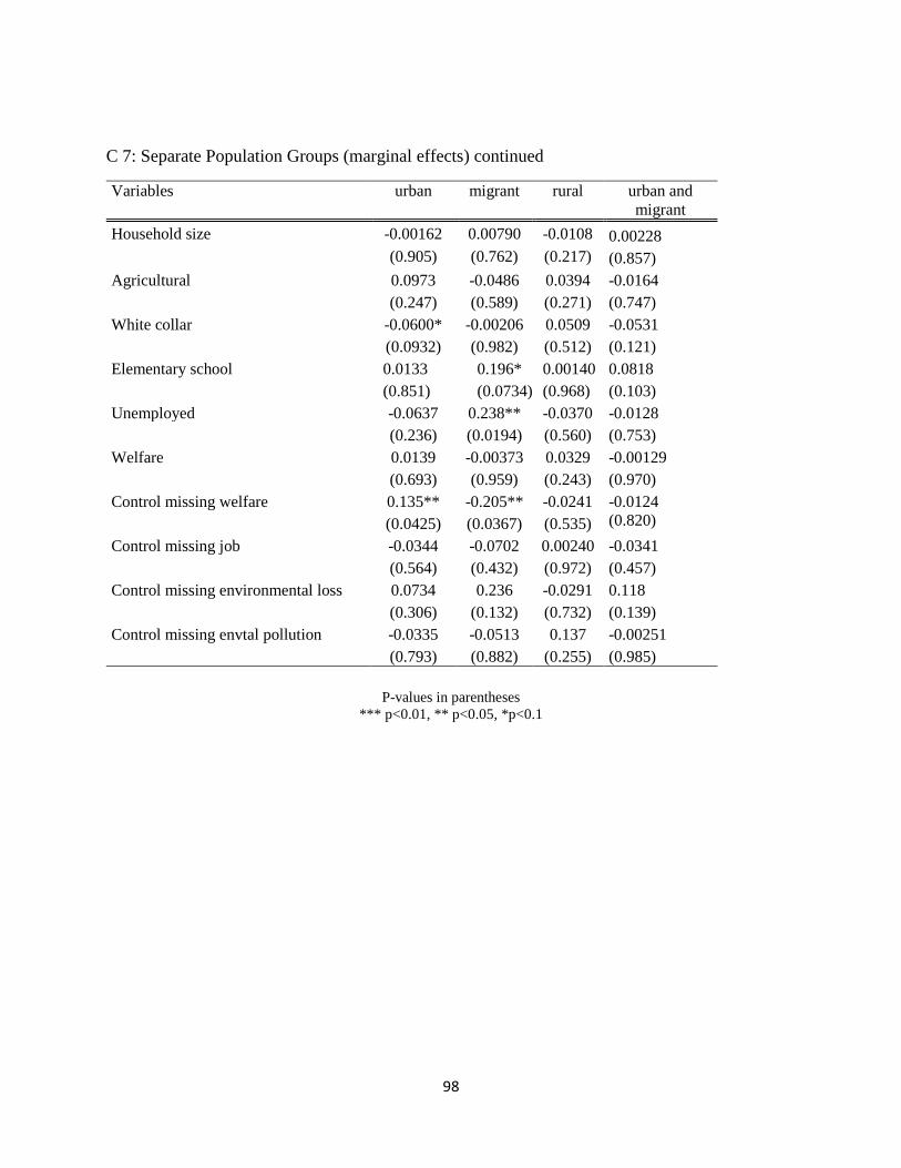
98

C 7: Separate Population Groups (marginal effects) continued

Variables urban migrant rural urban and

migrant

Household size -0.00162 0.00790 -0.0108 0.00228

(0.905) (0.762) (0.217) (0.857)

Agricultural 0.0973 -0.0486 0.0394 -0.0164

(0.247) (0.589) (0.271) (0.747)

White collar -0.0600* -0.00206 0.0509 -0.0531

(0.0932) (0.982) (0.512) (0.121)

Elementary school 0.0133 0.196* 0.00140 0.0818

(0.851) (0.0734) (0.968) (0.103)

Unemployed -0.0637 0.238** -0.0370 -0.0128

(0.236) (0.0194) (0.560) (0.753)

Welfare 0.0139 -0.00373 0.0329 -0.00129

(0.693) (0.959) (0.243) (0.970)

Control missing welfare 0.135** -0.205** -0.0241 -0.0124

(0.0425) (0.0367) (0.535) (0.820)

Control missing job -0.0344 -0.0702 0.00240 -0.0341

(0.564) (0.432) (0.972) (0.457)

Control missing environmental loss 0.0734 0.236 -0.0291 0.118

(0.306) (0.132) (0.732) (0.139)

Control missing envtal pollution -0.0335 -0.0513 0.137 -0.00251

(0.793) (0.882) (0.255) (0.985)

P-values in parentheses

*** p<0.01, ** p<0.05, *p<0.1

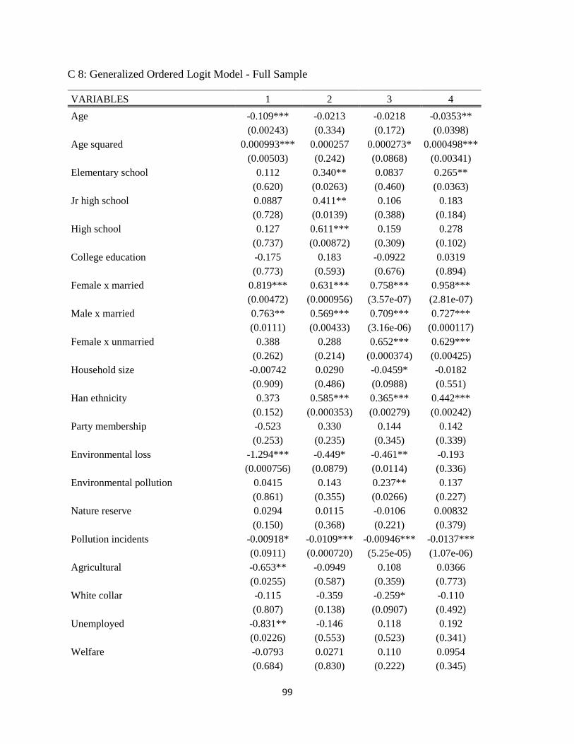
99

C 8: Generalized Ordered Logit Model - Full Sample

VARIABLES 1 2 3 4

Age -0.109*** -0.0213 -0.0218 -0.0353**

(0.00243) (0.334) (0.172) (0.0398)

Age squared 0.000993*** 0.000257 0.000273* 0.000498***

(0.00503) (0.242) (0.0868) (0.00341)

Elementary school 0.112 0.340** 0.0837 0.265**

(0.620) (0.0263) (0.460) (0.0363)

Jr high school 0.0887 0.411** 0.106 0.183

(0.728) (0.0139) (0.388) (0.184)

High school 0.127 0.611*** 0.159 0.278

(0.737) (0.00872) (0.309) (0.102)

College education -0.175 0.183 -0.0922 0.0319

(0.773) (0.593) (0.676) (0.894)

Female x married 0.819*** 0.631*** 0.758*** 0.958***

(0.00472) (0.000956) (3.57e-07) (2.81e-07)

Male x married 0.763** 0.569*** 0.709*** 0.727***

(0.0111) (0.00433) (3.16e-06) (0.000117)

Female x unmarried 0.388 0.288 0.652*** 0.629***

(0.262) (0.214) (0.000374) (0.00425)

Household size -0.00742 0.0290 -0.0459* -0.0182

(0.909) (0.486) (0.0988) (0.551)

Han ethnicity 0.373 0.585*** 0.365*** 0.442***

(0.152) (0.000353) (0.00279) (0.00242)

Party membership -0.523 0.330 0.144 0.142

(0.253) (0.235) (0.345) (0.339)

Environmental loss -1.294*** -0.449* -0.461** -0.193

(0.000756) (0.0879) (0.0114) (0.336)

Environmental pollution 0.0415 0.143 0.237** 0.137

(0.861) (0.355) (0.0266) (0.227)

Nature reserve 0.0294 0.0115 -0.0106 0.00832

(0.150) (0.368) (0.221) (0.379)

Pollution incidents -0.00918* -0.0109*** -0.00946*** -0.0137***

(0.0911) (0.000720) (5.25e-05) (1.07e-06)

Agricultural -0.653** -0.0949 0.108 0.0366

(0.0255) (0.587) (0.359) (0.773)

White collar -0.115 -0.359 -0.259* -0.110

(0.807) (0.138) (0.0907) (0.492)

Unemployed -0.831** -0.146 0.118 0.192

(0.0226) (0.553) (0.523) (0.341)

Welfare -0.0793 0.0271 0.110 0.0954

(0.684) (0.830) (0.222) (0.345)

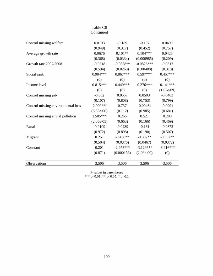
100

Table C8

Continued

Control missing welfare 0.0193 -0.189 -0.107 0.0490

(0.949) (0.317) (0.452) (0.757)

Average growth rate 0.0676 0.101** 0.104*** 0.0425

(0.368) (0.0334) (0.000985) (0.209)

Growth rate 2007/2008 -0.0318 -0.0888** -0.0826*** -0.0317

(0.594) (0.0268) (0.00408) (0.318)

Social rank 0.904*** 0.867*** 0.597*** 0.457***

(0) (0) (0) (0)

Income level 0.815*** 0.449*** 0.276*** 0.141***

(0) (0) (0) (1.02e-09)

Control missing job -0.602 0.0557 0.0503 -0.0463

(0.107) (0.808) (0.753) (0.799)

Control missing environmental loss -2.900*** 0.737 -0.00464 -0.0991

(3.55e-06) (0.112) (0.985) (0.681)

Control missing envtal pollution 3.505*** 0.266 0.521 0.289

(2.05e-05) (0.663) (0.166) (0.469)

Rural -0.0109 -0.0239 -0.161 -0.0872

(0.972) (0.898) (0.190) (0.507)

Migrant 0.251 -0.438** -0.302** -0.357**

(0.504) (0.0376) (0.0467) (0.0372)

Constant 0.201 -2.973*** -3.129*** -3.916***

(0.871) (0.000156) (2.08e-09) (0)

Observations 3,506 3,506 3,506 3,506

P-values in parentheses

*** p<0.01, ** p<0.05, * p<0.1

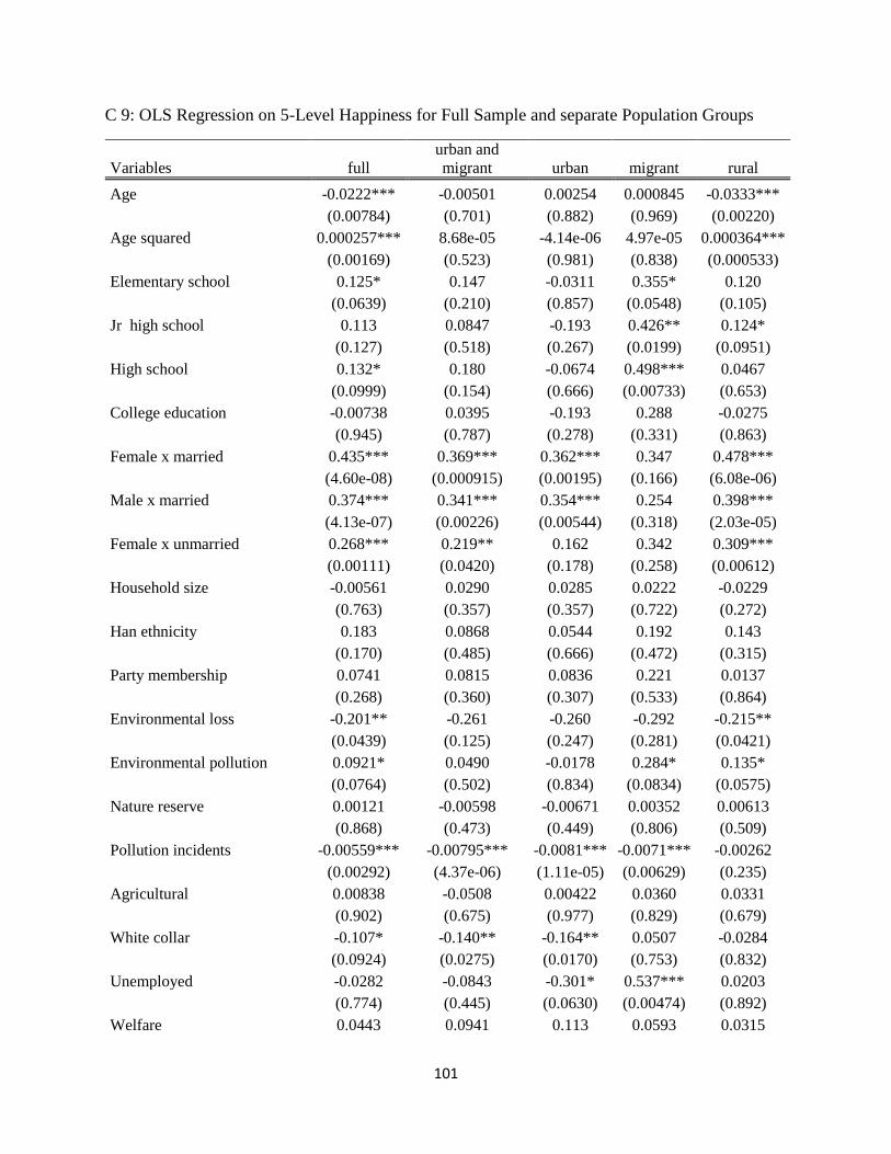
101

C 9: OLS Regression on 5-Level Happiness for Full Sample and separate Population Groups

Variables full

urban and

migrant urban migrant rural

Age -0.0222*** -0.00501 0.00254 0.000845 -0.0333***

(0.00784) (0.701) (0.882) (0.969) (0.00220)

Age squared 0.000257*** 8.68e-05 -4.14e-06 4.97e-05 0.000364***

(0.00169) (0.523) (0.981) (0.838) (0.000533)

Elementary school 0.125* 0.147 -0.0311 0.355* 0.120

(0.0639) (0.210) (0.857) (0.0548) (0.105)

Jr high school 0.113 0.0847 -0.193 0.426** 0.124*

(0.127) (0.518) (0.267) (0.0199) (0.0951)

High school 0.132* 0.180 -0.0674 0.498*** 0.0467

(0.0999) (0.154) (0.666) (0.00733) (0.653)

College education -0.00738 0.0395 -0.193 0.288 -0.0275

(0.945) (0.787) (0.278) (0.331) (0.863)

Female x married 0.435*** 0.369*** 0.362*** 0.347 0.478***

(4.60e-08) (0.000915) (0.00195) (0.166) (6.08e-06)

Male x married 0.374*** 0.341*** 0.354*** 0.254 0.398***

(4.13e-07) (0.00226) (0.00544) (0.318) (2.03e-05)

Female x unmarried 0.268*** 0.219** 0.162 0.342 0.309***

(0.00111) (0.0420) (0.178) (0.258) (0.00612)

Household size -0.00561 0.0290 0.0285 0.0222 -0.0229

(0.763) (0.357) (0.357) (0.722) (0.272)

Han ethnicity 0.183 0.0868 0.0544 0.192 0.143

(0.170) (0.485) (0.666) (0.472) (0.315)

Party membership 0.0741 0.0815 0.0836 0.221 0.0137

(0.268) (0.360) (0.307) (0.533) (0.864)

Environmental loss -0.201** -0.261 -0.260 -0.292 -0.215**

(0.0439) (0.125) (0.247) (0.281) (0.0421)

Environmental pollution 0.0921* 0.0490 -0.0178 0.284* 0.135*

(0.0764) (0.502) (0.834) (0.0834) (0.0575)

Nature reserve 0.00121 -0.00598 -0.00671 0.00352 0.00613

(0.868) (0.473) (0.449) (0.806) (0.509)

Pollution incidents -0.00559*** -0.00795*** -0.0081*** -0.0071*** -0.00262

(0.00292) (4.37e-06) (1.11e-05) (0.00629) (0.235)

Agricultural 0.00838 -0.0508 0.00422 0.0360 0.0331

(0.902) (0.675) (0.977) (0.829) (0.679)

White collar -0.107* -0.140** -0.164** 0.0507 -0.0284

(0.0924) (0.0275) (0.0170) (0.753) (0.832)

Unemployed -0.0282 -0.0843 -0.301* 0.537*** 0.0203

(0.774) (0.445) (0.0630) (0.00474) (0.892)

Welfare 0.0443 0.0941 0.113 0.0593 0.0315

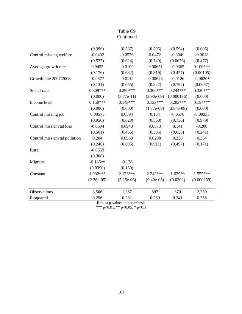
102

Table C9

Continued

(0.396) (0.287) (0.295) (0.594) (0.606)

Control missing welfare -0.0432 -0.0576 0.0472 -0.304* -0.0618

(0.537) (0.624) (0.749) (0.0676) (0.477)

Average growth rate 0.0455 -0.0109 -0.00651 -0.0365 0.106***

(0.176) (0.682) (0.819) (0.427) (0.00105)

Growth rate 2007/2008 -0.0377 -0.0112 -0.00643 -0.0126 -0.0620*

(0.131) (0.655) (0.822) (0.792) (0.0657)

Social rank 0.309*** 0.290*** 0.306*** 0.244*** 0.320***

(0.000) (5.77e-11) (2.90e-09) (0.000186) (0.000)

Income level 0.150*** 0.149*** 0.123*** 0.203*** 0.154***

(0.000) (0.000) (1.77e-08) (3.84e-08) (0.000)

Control missing job 0.00575 0.0594 0.104 -0.0576 -0.00335

(0.950) (0.623) (0.568) (0.736) (0.979)

Control miss envtal loss -0.0694 0.0943 0.0573 0.141 -0.200

(0.501) (0.465) (0.595) (0.658) (0.241)

Control miss envtal pollution 0.204 0.0950 0.0298 0.258 0.354

(0.240) (0.696) (0.911) (0.497) (0.171)

Rural -0.0659

(0.308)

Migrant -0.185** -0.128

(0.0390) (0.160)

Constant 1.932*** 2.123*** 2.242*** 1.629** 1.555***

(2.36e-05) (5.25e-06) (9.40e-05) (0.0302) (0.000269)

Observations 3,506 1,267 897 370 2,239

R-squared 0.256 0.281 0.269 0.341 0.258 Robust p-values in parenthesis

*** p<0.01, ** p<0.05, * p<0.1

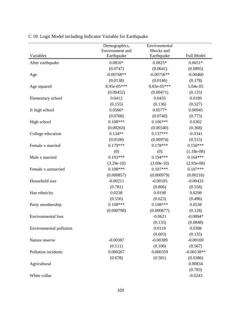
103

C 10: Logit Model including Indicator Variable for Earthquake

Variables

Demographics,

Environment and

Earthquake

Environmental

Shocks and

Earthquake Full Model

After earthquake 0.0810* 0.0825* 0.0651*

(0.0747) (0.0641) (0.0895)

Age -0.00768** -0.00756** -0.00460

(0.0138) (0.0146) (0.178)

Age squared 8.95e-05*** 8.83e-05*** 5.04e-05

(0.00452) (0.00471) (0.135)

Elementary school 0.0412 0.0435 0.0189

(0.155) (0.136) (0.527)

Jr high school 0.0566* 0.0577* 0.00945

(0.0768) (0.0740) (0.773)

High school 0.108*** 0.106*** 0.0302

(0.00263) (0.00340) (0.368)

College education 0.134** 0.137*** -0.0341

(0.0108) (0.00974) (0.515)

Female x married 0.179*** 0.178*** 0.150***

(0) (0) (1.18e-08)

Male x married 0.193*** 0.194*** 0.164***

(3.29e-10) (3.69e-10) (2.93e-08)

Female x unmarried 0.108*** 0.107*** 0.107***

(0.000857) (0.000979) (0.00216)

Household size -0.00211 -0.00185 -0.00433

(0.781) (0.806) (0.558)

Han ethnicity 0.0238 0.0198 0.0298

(0.556) (0.623) (0.496)

Party membership 0.108*** 0.108*** 0.0538

(0.000798) (0.000877) (0.128)

Environmental loss -0.0621 -0.0894*

(0.135) (0.0848)

Environmental pollution 0.0119 0.0398

(0.603) (0.135)

Nature reserve -0.00387 -0.00389 -0.00169

(0.111) (0.106) (0.567)

Pollution incidents 0.000267 0.000359 -0.00138**

(0.678) (0.581) (0.0386)

Agricultural 0.00834

(0.783)

White collar -0.0243

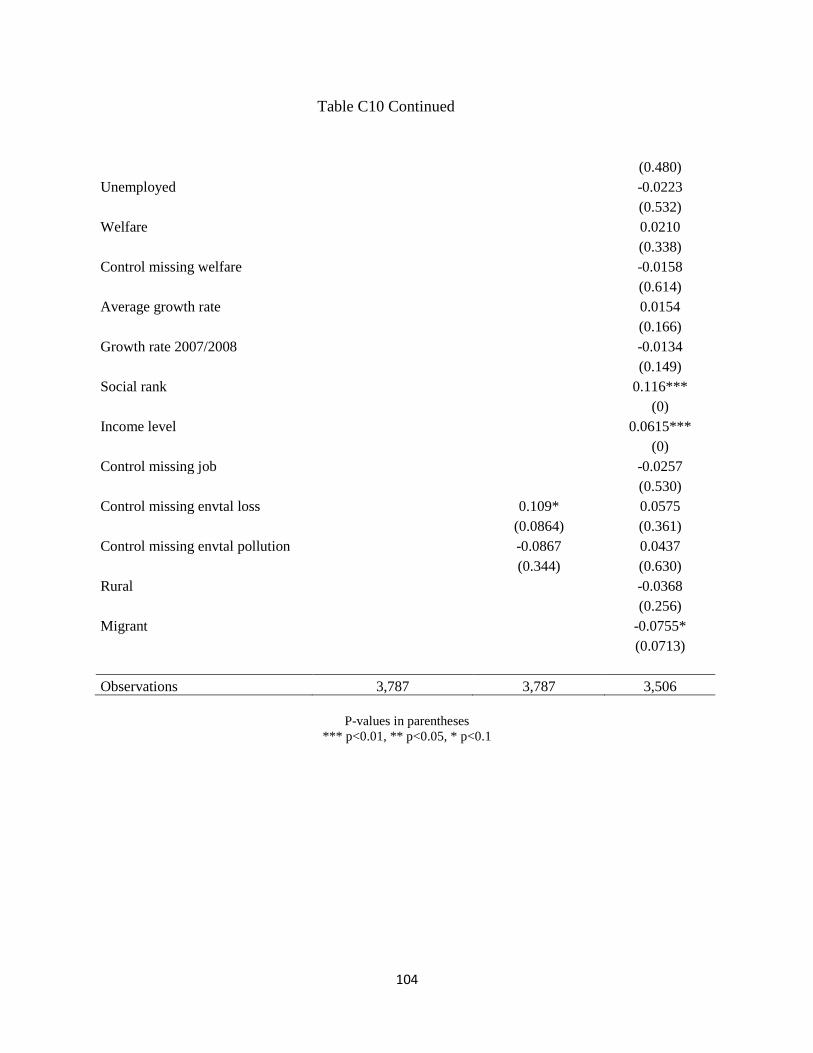
104

Table C10 Continued

(0.480)

Unemployed -0.0223

(0.532)

Welfare 0.0210

(0.338)

Control missing welfare -0.0158

(0.614)

Average growth rate 0.0154

(0.166)

Growth rate 2007/2008 -0.0134

(0.149)

Social rank 0.116***

(0)

Income level 0.0615***

(0)

Control missing job -0.0257

(0.530)

Control missing envtal loss 0.109* 0.0575

(0.0864) (0.361)

Control missing envtal pollution -0.0867 0.0437

(0.344) (0.630)

Rural -0.0368

(0.256)

Migrant -0.0755*

(0.0713)

Observations 3,787 3,787 3,506

P-values in parentheses

*** p<0.01, ** p<0.05, * p<0.1