PhD Thesis No. 150

Essays in the Economics of Transport

by

Jens Erik Nielsen

March 2007 Department of Economics University of Copenhagen

Studiestraede 6, DK-1455 Copenhagen www.econ.ku.dk

Essays in the Economics of Transport

Jens Erik Nielsen

Danish Transport Research Institute

and

University of Copenhagen

Ph.D. Dissertation

Department of Economics

University of Copenhagen

December 2006

- 1 -

Preface and Acknowledgments

The content of this thesis constitute my Ph.D. dissertation submitted to the Department of

Economics, University of Copenhagen in December 2006.

My Ph.D. scholarship has been financed by the Danish Transport Research Institute

(DTF); which is a research institute financed by the Danish Ministry of Transport and

Energy. I am thankful for their support and encouragement.

I would like to thank my supervisors Professor Peter Birch Sørensen from the University

of Copenhagen and Senior Researcher Mogens Fosgerau from the Danish Transport

Research Institute for their guidance and advice. I would also like to thank Professor

Christian Schultz who I got to know both as a member of the Ph.D. study board and

during many workshops, both domestic and abroad. I am especially indebted to

Researcher Ninette Pilegaard from the Danish Transport Research Institute with whom I

have had many interesting and motivating discussions. I hope we will keep in touch in the

future.

In 2004 I visited Lüdwig-Maxmillian Universität Munchen as a Marie Curie Fellow. I

would like to take this opportunity to thank the people from LMU and especially

Professor Ray Rees for making me feel welcome and at home in his department.

- 2 -

Special thanks also goes to my fellow Ph.D. students Elisabeth Herman Frederiksen and

Ri Kaarup who have helped improve my poor English, giving me valuable feedback on

my work, and making the time as a Ph.D. student more enjoyable.

Lastly I would like to thank my family and friends for their support during the last couple

of years. I know that my late grandmother would have loved the idea of having a doctor

in the family even though she would not know the difference between a doctor in

economics and a medical doctor.

Jens Erik Nielsen

Copenhagen, December 2006.

- 3 -

Changes since the dissertation was submitted

Since the dissertation was submitted in December 2006 and the public defense which

took place in Marts 2007 a few things have happened. First, a revised version of paper 1

titled ‘Externalities, taxation and time allocation’ has been accepted for publication in the

International Journal of Transport Economics. Secondly, it has been brought to my

attention that there were some typing mistakes in paper 3 and paper 4. These have been

corrected in the present version of the dissertation.

Jens Erik Nielsen

Copenhagen, April 2007.

- 4 -

Table of Contents Preface and acknowledgments

Changes since the dissertation was submitted

Table of Contents

Summary and introduction

Paper 1

Taxation, Time Allocation, and externalities

Paper 2

Estimation of car ownership in Denmark - Discrete choice modeling and

repeated cross-section analysis

Paper 3

Real estate ownership and the demand for cars in Denmark - A pseudo-

panel analysis

Paper 4

Demand for car transport in Denmark- Differences between rural and

urban car owners

Paper 5

Transport tax reforms, two-part tariffs, and revenue recycling

1

3

4

5

13

37

77

113

137

- 5 -

Summary and Introduction

The purpose of this introduction is to summarize the five papers that constitute this thesis.

Each paper is self-contained and can be read independently of the others but they all

centers around the same theme; the economics of transport. Papers one and five are

theoretical dealing with questions related to the theory of taxation. The remaining three

are empirical and centers on the estimation of car ownership and the use of cars in

Denmark.

The first paper, Taxation, Time Allocation, and Externalities, derives the optimal tax

rules in a model of household time allocation and atmospheric externalities based on

Becker (1965). In a situation without externalities and without distributional

considerations the optimal tax structure in such a setting is derived in Kleven (2004). We

extend on his findings in two ways. First, we include atmospheric externalities thus

generalizing the model making it more in line with the situation found in the transport

sector. Secondly we allow households to differ and implement a more general social

welfare function than the one used by Kleven thereby introducing distributional

considerations in the setup.

We show that the additivity property derived in Sandmo (1975) survives in the present

setup, even though it has to be modified to cope with distributional issues and time

allocation. We show that the definition of the net social marginal utility of income

defined in Diamond (1975) enters the optimal tax formula in a modified form which

includes income effects on the externality. Since the modified net social marginal utility

- 6 -

of income enters the tax formula for both polluting and non-polluting goods the additivity

property in the pure form, where the tax on non-polluting goods are independent of the

externality fails. We show that the substitution effects still enters the tax formula for the

externality generating good in an additive way and the additivity property thus survives

in a modified form. Furthermore we find that the factor share for the polluting good also

enters the additive term and the corrective term therefore no longer equals the pigouvian

marginal cost.

The policy implications of the insights obtained are obvious. As in Kleven (2004) we

show that fast modes of transport should be taxed less than slow modes and that the

modified additivity property states that a corrective tax should be levied on the polluting

good only. The optimal corrective tax is not equal to the pigouvian level found in

Sandmo (1975) since the time allocation has to be accounted for. If two modes pollute at

the same level the corrective tax on the fastest mode should be set at a lower rate than the

one at the slow mode.

The result from this paper addresses the present policy debate regarding taxation of

aviation fuel according to the emission of greenhouse gasses (CO2). Lately the Danish

minister of the environment, Connie Hedegaard, has argued that airline traffic should be

taxed according to the pigouvian principle since it emits large quantities of greenhouse

gasses compared to car transport. Using the results presented in paper 1 we know that this

argument is not a clear-cut case. It might be true that airline traffic emit higher quantities

of greenhouse gasses but it is also true that for many trips it saves time to use airlines

- 7 -

instead of cars. Our result states that if the time savings are high enough there is an

argument for having lower emission taxes on airlines than on cars. How the taxes are to

be set is an empirical matter which the paper does not address.

The second paper, Estimation of car ownership in Denmark - Discrete choice modeling

and repeated cross-section analysis, examines the demand for cars in Denmark by using

simple cross-section method. In this paper the problem of parameter instability in such

models are addressed and we hypothesizes that omission of a variable for household

wealth in the form of real estate values causes the estimates of income elasticities to be

upward biased.

To examine this we follow the same path as Pendyala et al. (1995) and use repeated

cross-section data to estimate a simple multinomial model for car ownership and examine

how the demand for cars evolves over time. The data used comes from the Danish

Transport Diary Survey which is an interview based survey conducted on a monthly

basis. The problem of parameter instability simple cross-section models is well known

and it is also known that the omission of important macro variables can cause estimated

parameters and elasticities to be biased. Due to lack of data one often has to relay on this

approach even though more sophisticated frameworks should be used. The problems

mentioned above therefore remains.

In the paper we find that the estimated income elasticities are non-decreasing over time,

which is expected from other studies. Furthermore we find that including a variable for

- 8 -

real estate values in the Danish municipalities reduce the estimated income elasticities. If

our hypothesis that the real estate values influence the demand for cars we should see the

largest changes in income elasticities for households who live in areas with the highest

values of real estate. By showing that the income elasticities for real estate owners in

urban areas are affected more than for other households and with real estate owners in

general being affected more by the inclusion of a variable for real estate values we

conclude that our hypothesis is correct.

The third paper extends on this finding and uses a dynamic model to examine the effect

of the housing prices in more detail.

In paper three, Real estate ownership and the demand for cars in Denmark - A pseudo-

panel analysis, the investigation of the influence of the rising real estate prices and the

falling interest rate, which was started in paper two, continues. Inspired by Dargay and

Vythoulkas (1999) we construct a dynamic partial adjustment model for car ownership in

Denmark. Using the approach described in Deaton (1985) we use data from the Danish

Transport Diary survey to construct a pseudo panel and combine this with aggregate time

series from Statistics Denmark for the development in real estate values in the Danish

municipalities and the development in the long-term interest rate. We hypothesis that the

increasing real estate values have increased the demand for cars and that the falling

interest rate also increase car demand.

- 9 -

With the rising real estate prices and the falling interest rate we have in Denmark a

situation where real estate owners can redraw equity from their real estate without

increasing their monthly expenses. These households have thus received a capital gain

which tenants have not and real estate owners could therefore have increased their

demand for cars. If this hypothesis is true we expect that the increasing housing prices

influence the demand for cars for real estate owners but not for tenants. The influence of

the interest rate is less clear since all households face approximately the same interest rate

if differences in capital restrictions are ignored. What we find is that only real estate

owners are affected by the increasing real estate prices but all households increase their

demand for cars due to the falling interest rate. Our hypothesis is thus confirmed.

Our findings in this paper is important since excluding capital gains from models used for

forecasting could cause estimates to be misleading. We have shown that future models

should keep this in mind and if possible include variables for capital gains and especially

gains originating from the real estate marked. Unfortunately we have not been able to

examine the effect of falling real estate prices and increasing interest rates. This should

be done since we should not expect the responses to be symmetric; a finding which

Dargay (2001) found with regards to income where hysteresis exist in the demand for

cars.

Paper four, Demand for car transport in Denmark- Differences between rural and urban

car owners, continues the investigation of differences between car owners in rural and

urban areas which was started in Dargay (2002). The paper contributes to the literature in

- 10 -

two ways. Since Dargay only used a constructed value for car travel derived from the UK

household expenditure survey one could question the validity of the results. By using a

transport survey and obtaining estimates which are comparable with Dargays results we

thus show that results obtained from household expenditure surveys can provide credible

results about transport behavior. Secondly we show that the purchase price and fuel

prices affects rural and urban households differently. This is an important insight since it

helps us to understand how different policies affect households living in different areas.

We show that rural households respond mostly to changes in the purchase price on cars

whereas urban households respond more to changes in fuel price (or variable costs).

The last paper, Transport tax reforms, two-part tariffs, and revenue recycling, construct

a model for commuting traffic. The consumers consume a composite commodity, leisure

and choose between public transport (a metro) and private transport (car) when they

commute. The model is thus based on the framework presented in Parry and Bento

(2001). The model extends on previous work by incorporating the discrete nature of car

purchase in a tax model which (to our knowledge) has not been done before.

- 11 -

References Becker (1965) A Theory of the Allocation of Time, The Economic Journal 75, 493-517.

Dargay, J. M and Vythoulkas, P. C. (1999) Estimation of a Dynamic Car Ownership

Model: A Pseudo-panel Approach, Journal of Transport Economics and Policy 33:3, 287-

302.

Dargay, J. M. (2001) The effect of income on car ownership: evidence and asymmetry,

Transportation Research Part A 35, 807-821.

Dargay, J. M. (2002) Determinants of car ownership in rural and urban areas: a pseudo-

panel analysis, Transportation Research Part E, 38, 351-366.

Deaton, A. (1985) Panel Data from Time Series of Cross Sections, Journal of

Econometrics 30, 109-126.

Diamond, P. A. (1975) A many-person Ramsey tax rule, Journal of Public Economics 4,

335-342.

Kleven, H. J. (2004) Optimum Taxation and the Allocation of Time, Journal of Public

Economics 88, 545-557.

Parry, I. W. H. & Bento, A. (2001) Revenue Recycling and the Welfare Effects of Road

Pricing, Scandinavian Journal of Economics 103:4, 645-671.

Pendyala, R. M., Kostyniuk, L. P. & Goulias, K. G. (1995) A repeated cross-sectional

evaluation of car ownership, Transportation 22, 165-184.

Sandmo, A. (1975) Optimal Taxation in the Presence of Externalities, Swedish Journal of

Economics.77, 86-97.

- 12 -

- 13 -

Taxation, Time Allocation, and Externalities

Jens Erik Nielsen

Danish Transport Research Institute

and

University of Copenhagen

Abstract

This paper shows that the traditional additivity property of Sandmo (1975) for taxation of

atmospheric externalities needs modification when household time allocation is modeled

in a Becker (1965) setup and it address the question of distributional consequences in a

model with explicit modeling of household time allocation. The insights obtained have

important policy implications in the transport sector, since we show that time saving

activities should have their externality tax reduced compared to the pure Pigouvian case.

The traditional arguments for marginal cost pricing thus looses some of its appeal.

- 14 -

1. Introduction

This paper models household time allocation in a setup with atmospheric externalities.

We assume that households require both household time and market produced

commodities in the production of consumption goods in line with Becker (1965). This

setup is particular relevant when the theory of optimal taxation is applied to the transport

sector since one of the main characteristics of transportation is the use of time.

Furthermore, personal transport produced by households takes up a large fraction of

household time budgets and transport is also a significant source of externalities. In a

situation without externalities and without distributional considerations the optimal tax

rules for the present setup is derived in Kleven (2004). He derives a so called inverse

factor share rule which state that activities with a high time share and thus a low factor

share in household production should be taxed at a higher rate than activities which a low

time share and a high factor share. The present paper extends this result by including

externalities and considering distributional concerns.

It is shown here that the additivity property found in Sandmo (1975) has to be modified

when household production and time allocation is modeled explicitly in the presence of

externalities. The additivity property states that if the externality generating good can be

taxed directly, efficiency requires that this good is taxed by combining the Pigouvian

principle and Ramsey taxation and that the externality level only enters the tax formula

for the externality generating good. The Pigouvian tax is additive thus making a clear

separation between the efficiency part of the tax formula and the part of the tax formula

which correct for the externalities. When the allocation of time in household production

- 15 -

is included in the setup we show that the corrective tax has to account not only for the

externalities but also for the time cost involved. This insight invalidates the conclusion

that the internalizing part of the tax should be set equal to the marginal external damage

costs. Furthermore we show that the definition of the net social marginal utility of income

defined in Diamond (1975) has to be modified to account for the negative welfare effects

of the externalities if distributional issues are included in the model.

Allowing for distributional issues in the economy does not invalidate the additivity

property but it has to be modified. We show that since the net social marginal utility of

income is modified to include the income effect on the level of the externality the

Ramsey part of the tax problem is no longer independent of the externality. The

corrective term containing substitution effects still enters additive in the tax formula for

the good causing externalities and the additivity property therefore remains valid.

It has almost become the convention in the transport sector that a system of road pricing

where the tax is set equal to the marginal external cost is the most efficient way to

internalize externalities. In the present setup this no longer holds. The tax should also

account for the time allocation inside the households. A direct consequence is that a

transport mode which saves time should carry a lower corrective tax even if the marginal

external damage costs for the different modes are the same. For example even if cars

cause more atmospheric pollution than busses the optimal corrective tax on cars might be

lower than the tax on busses. This can happen if the time saved from using the car is high

enough. The insight can also be applied to the taxation of airlines where politicians are

- 16 -

discussing if a tax should be put on aviation fuel in order to reduce the emission of

greenhouse gasses. Since air transport in general saves time compared to other modes of

transport our result says that the internalizing tax should be set lower on aviation fuel

relative to fuel used in car transport even if the marginal damage caused by the two

modes are the same.

Similar insights concerning pigouvian taxation are obtained from a different setup in

Parry and Bento (2001). They analyze tax reforms in a simple labor-leisure model with

two types of transport to show that when distortions on the labor market are included it

might not be welfare improving to internalize externalities by setting the tax equal to the

marginal external damage cost. Using their model they investigate different tax reforms

in the transport sector and use numerical simulation to illustrate their results. The Parry

and Bento result is extended in several recent papers. In Parry and Bento (2002) they

extend their analysis and investigate more types of externalities and interactions with

other taxes. De Borger and Van Dender (2003) show, using the same framework as Parry

and Bento, that the value of time is also affected by the tax system and in Nielsen (2006)

the setup is extended to include the discrete choice of car purchase.

None of the above mentioned papers derive optimal tax rules in models with time

allocation and externalities. This paper thus contributes to the literature by deriving the

optimal tax rule in a model with explicit modeling of household time allocation,

atmospheric externalities, and by including distributional considerations.

- 17 -

The paper is organized as follows. Section 2 sets up the model describing the households'

time allocation problem and the governments’ problem of raising revenue. Section 3

derives the optimal tax rules and the final section concludes.

2. The Model

As in the standard setup the model used here includes a utilitarian social planner and a set

of H households together with N+1 commodities. Households do not consume

commodities bought in the market directly. Instead they undertake a production where

market produced commodity, iX , and household time, iL , are used to produce

consumption good, iZ , through a production process, if . Letting h describe the

individual household, they each have a utility function given by

0 1( , ,..., ) ( ), 1,...,h h h h h hNNU U Z Z Z Z h Hφ= − = (1)

where

1

Hh

N Nh

Z Z=

= ∑ (2)

is the total consumption of good N in the economy and

( , ), 0,...,h i h hi i iZ f X L i N= = (3)

represents the way good hiZ is being produced in household h using market produced

commodity, hiX , household time, h

iL , and production technology, if . The production

technologies, if , are Leontief and every household uses the same set of technologies

when producing consumption goods. This means that if a household wants to see a movie

at a cinema they have to allocate the time required to see the movie and they have to

purchase movie tickets. One could argue that more than one commodity could be

- 18 -

required in the production which would result in iX being a vector of these market

produced commodities, but to keep things simple we assume that only one commodity

goes into the production of every consumption good1.

In this setup the consumption of good N generates externalities. It is assumed that total

consumption of good N and not only total consumption of market produced commodities

that causes externalities. Considering transport as the main example in this paper, this is

the intuitive choice and changing it will not affect the conclusions. The function ( )hNZφ

is assumed to be increasing in NZ so that

( )' 0h h NN

ZZ

φφ ∂∂= > (4)

As a result the total consumption of good N decreases the utility of the households.

Assuming that H is large the households consider NZ as fixed when making their

choices. We therefore make the standard assumption that the individual household

behaves as if 0NhN

ZZ

∂∂

= . This means that a household may realize that it affects the total

consumption of good N but regards its contribution as insignificant. Using this we now

formulate the optimization problem for household h as

0 0

0 10 0 1 1

,..., , ,...,

0

0

max ( ( , ), ( , ),..., ( , ))

. .

h h h hN N

h h h h h N h hN N

X X L L

Nh h h

i iiN

h hi

i

U f X L f X L f X L

s t

P X w T

L T T

=

=

=

+ =

∑

∑

(5)

1 A discussion of this can be found in Pollak and Wachter (1975).

- 19 -

where hT is the amount of time spent on work for household h, iP is the consumer price

of commodity i, T is the total time available to the households, and hw is the wage rate

for household h and given exogenously. Since NZ is considered to be constant we can

leave out ( )hNZφ of the utility maximization problem (5).

The household production problem describing the way in which households choose hiX

and hiL in order to produce one unit of consumption good h

iZ in the cheapest possible

way can be formulated as

,min

. .( , ) 1

h hi i

h h hi i i

X L

i h hi i

P X w L

s tf X L

+

=

(6)

Due to the Leontief production technology the solution to (6) gives the constant factor

demand coefficients

Xi

hihi

XZ

a = (7)

Li

hihi

LZ

a = (8)

These are identical for all households since they use identical technologies. Using (7) and

(8) together with the fact that the two constraints in (5) are interdependent through the

variable hT , we can restate the households maximization problem as

00 1

,...,

0

max ( , ,..., )

. .

( , ) ( )

h hN

h h h hN

Z Z

Nh h h h hi i i

i

U Z Z Z

s t

Q P w Z I w=

=∑

(9)

- 20 -

where ( )h h hI w w T= is the households total income and ( , )h h hi i i Xi LiQ P w Pa w a= + . To

see this remember that Xia and Lia are constant and identical for all households.

Multiplying the time constraint in (5) with hw and adding it to the budget constraint in

(5) gives (9). Note that i XiPa is the direct monetary cost of using hiX as input and h

Liw a

is the value of the time used for the production which equals the earnings lost due to

lower working time2. ( , )h hi iQ P w is therefore the total opportunity cost of consuming one

unit of hiZ for household h.

With (9) being a standard utility maximization problem the solution gives the ordinary

demand functions 0 1( , ,..., , )h h h h hi NZ Q Q Q I and the indirect utility function

0 1( , ,..., , )h h h h hNV Q Q Q I . Note that the households’ indirect utility function does not include

externalities. We also know that standard results like Roy's Identity, which states that

, 0,...,h hk

hhk

VQ

Z k Nλ∂∂

= − = (10)

will apply where hλ is the Lagrangian multiplier from the households utility

maximization problem (9) and thus equals marginal utility of income for consumer h. We

also know that the Slutsky equation

, , 0,...,hj

hh hk k kh h hj j

Z ZZQ Q I

Z j k N∂ ∂∂∂ ∂ ∂

= − = (11)

holds where hkZ is the compensated demand function for good k.

2 We have assumed that the value of time is equal to the wage rate. A large literature on the value of time exists and it is one of the main research areas in transport economics. A recent Danish publication on the topic of time values is Fosgerau and Pilegaard (2003) which also contains a survey of the time value literature.

- 21 -

Having characterized the households’ behavior, we now focus on the government. The

government knows that externalities are present and it therefore know that the true

indirect utility function for household h is given by

0 1 0 1 0 11

( , ,..., , ) ( , ,..., , ) ( ( , ,..., , ))Hh h h h h h h h h h h h h h h

N N N Nh

V Q Q Q I V Q Q Q I Z Q Q Q Iφ=

= − ∑ (12)

We assume that the government seeks to maximize a Bergson-Samuelson type social

welfare function 1 2

( , ,..., )H

W W V V V= where 0hWV∂∂

> . Assuming that the production

sector operates under constant returns to scale and that all markets are fully competitive

the producer price, ip , for commodity iX is fixed and equal to the marginal cost of

production. We assume that good 0 is pure leisure and thus having 0 0Xa = making good

0 untaxable since no market produced commodity is used in the production of 0Z . We

define the tax rate on commodity iX as

, 1,...,i i it P p i N= − = (13)

The government therefore has full control of all commodity prices. Furthermore the

government must raise an externally given revenue, G, for some unspecified tasks (e.g.

defense, healthcare, infrastructure) resulting in the governmental budget constraint

0 1

( )N H

hi i

i h

t X G= =

=∑ ∑ (14)

We can now write the governments welfare maximization problem as

1 2

0 1

, ,...,

1 1

max ( , ,..., )

. .

(( ) )

N

H

P P P

N Hh

i i Xi ii h

W V V V

s t

P p a Z G= =

− =∑ ∑

(15)

- 22 -

since h hXi i ia Z X= and 0 0Xa = . The Lagrangian function emerging from (15) is given by

0 1

1 1

( , ,..., ) (( )( ) )N HH h

i i Xi ii h

L W V V V P p a Z Gµ= =

= + − −∑ ∑

(16)

where µ is the Lagrangian multiplier from (15) and representing marginal value of

government funds. The first order conditions for the governments welfare maximization

problem (15) can now be written as

1 1

1 1 1

( )

0, 1,...,

H H

h h

H N Hh

Xk k i Xih i h

h hhhh k N kh h hNk k kk k

hhi kh kk

Q QZL W VP P PZQ QV

QZPQ

a Z t a k N

φ

µ µ

= =

= = =

∂ ∂∂∂∂ ∂ ∂∂ ∂ ∂∂∂ ∂∂

∂∂∂∂

= −

+ + = =

∑ ∑

∑ ∑ ∑

(17)

which (by using Roy's identity (10) and the fact that hk

k XkQP a∂∂ = ) can be written as

1 1 1 11

(( ) ' ) , 1,...,H H H N H

h h h hk k i Xi

h h i hh

h hN i

h hhkk

Z ZWQQV

Z Z t a k Nλ φ µ µ= = = ==

∂ ∂∂∂∂∂

− − = − − =∑ ∑ ∑ ∑ ∑ (18)

Applying the Slutsky Equation (11) now gives

1 1 1

1 1 1

( ) ' ( )

( ), 1,...,

H H Hh h h h

k kh h h

H N Hh hk i Xi k

h i h

h hN N

h h h hk

h hi Nh hk

ZZW WQ IV V

ZZQ I

Z Z

Z t a Z k N

λ φ

µ µ

= = =

= = =

∂∂∂ ∂∂ ∂∂ ∂

∂∂∂ ∂

− − −

= − − − =

∑ ∑ ∑

∑ ∑ ∑

(19)

Following Diamond and Mirrlees (1971) and Diamond (1975) we define the social

marginal utility of income hβ and the net social marginal utility of income h

β for

household h as

h hh

WV

β λ∂∂

= (20)

1

Nh hi Xi

i

hih

ZI

t aβ β µ=

∂∂

= + ∑ (21)

- 23 -

We see that hβ is the social value of increasing the utility of consumer h by increasing

his budget. But if his budget is increased he will change his consumption pattern which

will result in a change in the tax payments. The second term in the definition of h

β

captures this effect and it is therefore the net social marginal utility of income for

consumer h. By using (20) the first order condition (19) can now be written as

1 1 1

1 1 1

' ( )

( ), 1,...,

H H Hh h h h

k kh h h

H N Hh hk i Xi k

h i h

h hN N

h h hk

h hi ih hk

ZZWQ IV

ZZQ I

Z Z

Z t a Z k N

β φ

µ µ

= = =

= = =

∂∂∂∂ ∂∂

∂∂∂ ∂

+ −

= + − =

∑ ∑ ∑

∑ ∑ ∑

(22)

By applying (21) and the symmetry of the derivative of the compensated demand

functions, h hi kh h

ik

Z ZQ Q∂ ∂∂ ∂

= , we can write (22) as

1 1 11 1

1 1 1

' ( )1 1 1 , 1,...,

h hH H hH N HZ Zh Zh h hN Nh kkh i Xik h h hQ I Qh h i ih k hH H H

h h hk k k

h h h

ZZ t a

Z Z Zk N

βλφβ

µ µ

∂ ∂ ∂

∂ ∂ ∂= = == =

= = =

−

+ = + =∑ ∑∑ ∑∑

∑ ∑ ∑

(23)

We now define the index of discouragement (Mirrlees (1976)) as

1 1

1

k

hN H Zki Xi hQi ih

Hhk

h

t a

Zd

∂

∂= =

=

=∑∑

∑

(24)

We see that i Xit a is the increase in generalized price, hiQ , caused by the tax. The

numerator therefore describes the total change in consumption of good k caused by

changing the price system. The denominator is the total consumption of good k and (24)

therefore measures the proportionate reduction in total consumption of good k caused by

the tax system. Using (24) we can write (23) as

- 24 -

( ) ( )

1 11

1 1

' ( )1 11 , 1,...,k

a b

hH H hH Z Zhh h hN Nh khk h hQ Ih hh kH H

h hk k

h h

ZZ

Z Zd k N

βλφβ

µ µ

∂ ∂

∂ ∂= ==

= =

−

= − + =∑ ∑∑

∑ ∑

(25)

This formula characterizes the optimal tax system in the economy. Knowing that the

compensated cross-price effects are positive the discouragement index is positive (if the

tax is positive). The right hand side of (25) capture the three goals of the tax system;

efficient generation of revenue, equity considerations, and internalization of externalities.

Part (a) of (25) is the standard Ramsey term3. The Ramsey result emerges in its most

simple form if we take (a) of (25), assume that all households are identical, and that no

externalities exist. This gives h

β β= and 0hφ = for all h and the tax rule can be written

as

1, 1,...,kd k Nβµ= − = (26)

saying that the taxes should be set in such a way that the index of discouragement is

identical for all goods. The Ramsey term (a) in (25) capture both efficiency and equity

considerations through h

β . To see this note that through 1

1

1

Hh h

kh

Hhk

h

Z

Z

β

µ=

=

∑

∑ we get that the

reduction in demand should be low when hβ is high, which happens for socially

important households. The second part of (a) given by 11

1

H N hZh ii Xik hIih

Hhk

h

Z t a

Z

∂

∂==

=

∑ ∑

∑ tells us that if

demand is consentrated among households where the tax payments are reduced

significantly when income change, then the reduction in demand should be kept low,

3 See for example Myles (1995) formula (4.40) and (4.44)

- 25 -

since a high reduction in demand will reduce tax revenue significantly thus calling for

even higher taxes to be set in order to meet the governments revenue requirement, which

will lead to even larger distortions

Part (b) of (25) deals with the externality. To simplify this we define

'h

hh

WV

β φ∂∂

= (27)

which, to keeping with the terminology, is the social marginal disutility of the externality

for household h. It measures how much social welfare change due to changes in the

utility for household h if the consumption of the externality generating good increases.

We see that households who are socially important (having a high value of hWV∂∂

) and who

are highly sensitive to changes in the externality level (having a high value of 'hφ ) will

have a high value of h

β . In a transport setting this could be the case for low-income

households living near the source of pollution (e.g. near large roads or near airports). We

see that from (4) and the definition of W, the social marginal disutility of the externality

is positive and higher values of h

β thus decrease welfare since it enters negatively in the

utility function for the households (1).

As in (2) we define 1

H hk kh

Z Z=

=∑ as the total consumption of good k and use it to write

(b) of (25) as

- 26 -

1 11 1

( ) ( )( ) (25)

1 1

1

( )1 1 1

h

H H H Hh h

h hh h

c db of

h hH H hh Z Z ZhN N kkh h hh hQ I Qh h k N k N

H k khk

h

ZZ Z

Z Z IZ

β

µ µ µβ β= == =

∂ ∂ ∂

∂ ∂ ∂= =

=

−∂∂

= −∑ ∑

∑∑ ∑ ∑ ∑

(28)

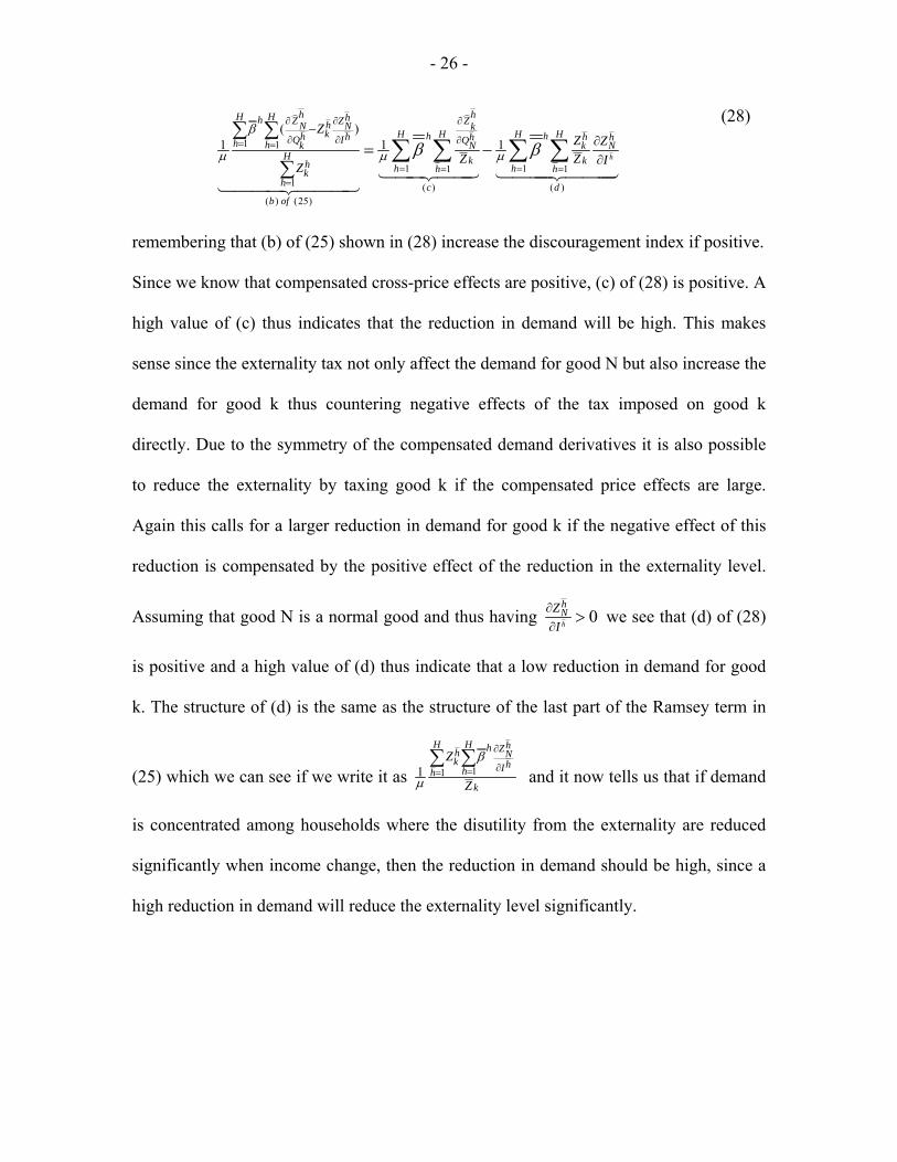
remembering that (b) of (25) shown in (28) increase the discouragement index if positive.

Since we know that compensated cross-price effects are positive, (c) of (28) is positive. A

high value of (c) thus indicates that the reduction in demand will be high. This makes

sense since the externality tax not only affect the demand for good N but also increase the

demand for good k thus countering negative effects of the tax imposed on good k

directly. Due to the symmetry of the compensated demand derivatives it is also possible

to reduce the externality by taxing good k if the compensated price effects are large.

Again this calls for a larger reduction in demand for good k if the negative effect of this

reduction is compensated by the positive effect of the reduction in the externality level.

Assuming that good N is a normal good and thus having 0h

hNZ

I∂∂

> we see that (d) of (28)

is positive and a high value of (d) thus indicate that a low reduction in demand for good

k. The structure of (d) is the same as the structure of the last part of the Ramsey term in

(25) which we can see if we write it as 111

H H hh Zh Nk hIhh

k

Z

Z

β

µ

∂

∂==∑ ∑

and it now tells us that if demand

is concentrated among households where the disutility from the externality are reduced

significantly when income change, then the reduction in demand should be high, since a

high reduction in demand will reduce the externality level significantly.

- 27 -

3. Tax rules

Since (25) only characterize the optimal tax system implicitly it is difficult to derive clear

policy implications from it. This section imposes further restrictions on the model to

derive some well known results and some new insights.

3.1 Inverse factor share rule and inverse elasticity rule

To obtain the inverse factor share rule we take (22) as a starting point. We assume that all

households are identical (giving us hβ λ= , hk kQ Q= , and h

k kZ Z= for all household), that

no externalities are present ( 0hφ = for all households), that the government maximizes

the unweighted sum of household utilities, and that no income effects exist since we are

not concerned with distributional issues. With these assumptions the first order conditions

for (15) reduces to

1

, 1,...,N

k i Xii

ik

ZQZ t a k Nλ µ

µ=

− ∂∂= =∑

(29)

Assuming that there are no compensated cross price effects between taxable goods in the

economy, and defining the constant

λ µµθ −= (30)

we can simplify (29) to

1 , 1,...,k Xkk

kk

ZZQt a k Nθ ∂

∂= = (31)

This allow us to write the optimal tax formulas as

1 , 1,...,k

kkk Xk

tP k Nα ε θ= = (32)

- 28 -

where k Xk

kXk

P aQα = is the factor share of kX and k k

kkkk

QZZQε ∂

∂= is the compensated own

price elasticity of commodity k (remembering that in optimum the value of compensated

and uncompensated demand are equal, k kZ Z= ). This is the inverse factor share rule

derived in Kleven (2004) saying that goods which use much household time in

production and hence have a low value of Xka (thus having a large time share4) should

carry a higher tax rate than goods which primarily use market-produced commodities in

the household production. The rationale behind this result is that since leisure time can

not be taxed directly the tax system causes a distortion on the labor market. If the

government taxes goods having a high time share in household production they therefore

reduce the distortion by taxing time indirectly through the production process. It is easy

to see that the inverse elasticity formula is imbedded in this formulation. Letting 1Xka =

for all households the model reduces to the standard model used in the analysis of

optimal taxation5 resulting in the inverse elasticity formula

, 1,...,kkkk

tP k Nθ

ε= = (33)

saying that goods with high compensated own-price elasticity should be taxed less than

goods with low compensated own-price elasticity in order to reduce distortions in the

consumption patterns. Lifting the assumption about identical treatment of the households

allows us to derive a more general version of the inverse factor share rule (32) where

distributional considerations are taken into account. We thus relax the assumption about

the government allowing it to maximize a more general welfare function and treat the

4 The time share of kX is given by 1Lk

kLk XkwaQα α= = − .

5 See Sandmo (1976) for an introduction.

- 29 -

households as being different (different utility functions and different income). Again we

start from (20) we write the first order condition as

1 1 1 1

( ), 1,...,H H N H

h h h hk k i Xi k

h h i h

h hi ih hk

ZZQ I

Z Z t a Z k Nβ µ µ= = = =

∂∂∂ ∂

= + − =∑ ∑ ∑ ∑ (34)

We assume that no cross-price effects exist between taxable goods. This allow us to write

(34) as

1

1

( ), 1,...,

H hhk

k hH hk h hkkk Xk

h

ZtP

Zk N

β µµ

ε α

−

=

=

= =∑

∑

(35)

where k Xkhk

hXk

P a

Qα = is the factor share of good k for household h. The insights from the

simple inverse factor share rule (32) still holds but we see that we now have to take

account of distributional concerns. It is easily recognized that ( )hβ µµ− is negative (if G is

positive) since µ is the Lagrangian from (15). With the compensated own-price

elasticity, kkε , also being negative we have that kk

tP is positive. Since high-income

households have higher generalized price, hkQ , their factor-share, h

Xkα , will be lower than

the factor-share for low-income households. To see this note that

( , )h h hi i i Xi LiQ P w Pa w a= + and that a higher value of hw gives a higher value of h

iQ . In

this situation the inverse factor share rule will benefit high-income households which is a

general dilemma in the transport sector when the value of time is assumed to be higher

for high-income households (and especially if the wage rate is used as a proxy for the

value of time as we do here). In such cases time-savings experienced by high-income

households weight more than the time savings experienced by low-income households.

- 30 -

The distributional considerations working through hβ pulls in the opposite direction and

if good k is consumed primarily by socially important households (normally low-income

households) the tax should be set at a low since h

β will be closer to µ for these

households thus bringing hβ µµ− closer to zero calling for a lower tax to be set.

3.3 The additivity property

When externalities are present we can derive the optimal tax rules by again taking (22) as

a starting point. Assuming that all households' are identical and that the government

maximizes the unweighted sum of the households utility. This gives the first order

conditions

1

1 1 1 , 1,...,N

k Xii

N iN k kk k

Z ZZ ZZ Q QH t a k Nλ µ φ

µ µ=

∂ ∂− ∂∂ ∂ ∂= − + =∑

(36)

This, by assuming that no compensated cross-price effects exist between taxable goods

and ignoring income effects, simplifies to

1

1 1

, 1,..., 1

,

k Xk

k Xk

ikk

i kk kk k k

ZZQ

Z ZHZ ZQ Z Q

t a k N

t a k Nφµ

θ

θ

∂∂

∂∂ ∂∂ ∂ ∂

= = −

= − =

(37)

giving the optimality conditions

1

1

(1 )( ), 1,..., 1

' (1 )( ) ',

kkk kkk Xk Xk

kkk kkk Xk k Xk kXk Xk

tP

t H HP Q Q

k N

k N

θα ε α ε

θα µ α λα ε α ε

ξ

φ ξ ξ φ

−

−

= = − = −

= + = − + =

(38)

where λµξ = . Note that since λ is the marginal value of private income and µ is the

marginal value of public income the parameter ξ can be interpreted as the marginal rate

of substitution between private and public income. The formulas for optimal taxation

- 31 -

consist of three elements. The first, 1Xkα , is the inverse factor share rule found in Kleven

(2004) stating that goods which has a low time share and thus a high factor share in the

household production process should be taxed less than other goods. The second, 1kkε

, is

the well known inverse elasticity rule stating that goods having low compensated own-

price elasticity should be taxed higher than goods with high compensated own-price

elasticity. The last element, ' 1Xkk

HaQ

φµ , is the additive term on the externality generating

good. With no explicit modeling of time (e.g. having 1=Xka for all k) it is just the

standard additive term found in Sandmo (1975) saying that the extra tax should be set

according to the principle for Pigouvian taxation. This no longer holds as the term 1Xkα

enters the formula. The tax rule now states that the social planner has to account for the

time allocation by taxing time saving activities at a lower rate even if these activities

generate negative externalities. In summary, the tax problem can be separated into two

parts. First, a tax is used to internalize externalities taking into consideration the time

allocation involved. Hereafter the government uses the inverse factor share rule to satisfy

its revenue requirement. The formula also tells us that in the event of 1ξ > where the

revenue generated from internalizing the externalities more than covers the government

revenue requirement and funds therefore have to be given back to the households. Note

that in the unlikely situation where 1ξ = the tax system will be first-best. In this situation

the government can finance its revenue requirement by using the corrective tax alone and

no other taxes are needed.

- 32 -

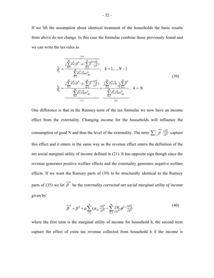
If we lift the assumption about identical treatment of the households the basic results

from above do not change. In this case the formulae combine those previously found and

we can write the tax rules as

( )

( ) ( )

1

1 1

1

1 1 1

1 11 1

1 1

( )

( )

, 1,..., 1

,

h

e

f g

H H hh Zh h Nk hIhk hH h hk hk kk Xk

hH H H Hh hZh hh hNk k kkh hI Qh h kk h h

H Hh hh hk h hk kkk kkXk Xkh h

ZtP

Z

Z ZtP

Z Z

k N

k N

µ

µ µ

β µ β

ε α

β µ β ε β

ε α ε α

∂

∂= =

=

∂

∂= == =

= =

− −

− −

= = −

= + =

∑ ∑

∑

∑ ∑ ∑ ∑

∑ ∑

(39)

One difference is that in the Ramsey-term of the tax formulas we now have an income

effect from the externality. Changing income for the households will influence the

consumption of good N and thus the level of the externality. The term 1

hH

h

hNh

ZI

β=

∂∂∑ capture

this effect and it enters in the same way as the revenue effect enters the definition of the

net social marginal utility of income defined in (21). It has opposite sign though since the

revenue generates positive welfare effects and the externality generates negative welfare

effects. If we want the Ramsey parts of (39) to be structurally identical to the Ramsey

parts of (35) we let h

β be the externality corrected net social marginal utility of income

given by

1 1

'N Hh h h

i Xii h

hhi Nh hh

ZZ WI IV

t aβ β µ φ= =

∂∂ ∂∂ ∂∂

= + −∑ ∑ (40)

where the first term is the marginal utility of income for household h, the second term

capture the effect of extra tax revenue collected from household h if the income is

- 33 -

increased, and the last term is the loss in welfare due to changes in the consumption of

good N by household h if the income is increased. Using this we can write (40) as

( )

( ) ( )

1

1

1

1 1111 1

1 1

( )

( )

, 1,..., 1

,

h

h

h

i j

H hk

k hH h hk hk kk Xk

hH HH hh hh

k kkk hQh kk h hH Hh hh hk h hk kkk kkXk Xk

h h

ZtP

Z

ZZtP

Z Z

k N

k N

µ

µµ

β µ

ε α

ε ββ µ

ε α ε α

=

=

== =

= =

−

−

= = −

= + =

∑

∑

∑ ∑∑

∑ ∑

(41)

where (h) and (i) of (40) is the familiar Ramsey term and has the same interpretation. Part

(j) of (40) is the corrective term of the tax formula and it still enters additive and this

additive term is the only part of (41) which incorporate substitution effects for good N.

The additivity property thus survives in the present setup.

4. Conclusion and possible extensions

In this paper we have presented a model of household behavior where time enters the

utility function directly as proposed in Becker (1965). Since the consumption of time is

very important in the transport sector the approach is a natural extension to the traditional

microeconomic setup when this sector is being modeled.

The tax rules found in the previous section help us to understand how the tax system

should be designed. If distributional considerations are ignored the inverse factor share

rule states that fast transportation should carry a lower rate of tax than slow

transportation. This conclusion is less clear when externalities are included because a

- 34 -

faster car might cause externalities that a slow car does not (for example accidents and

pollution).

Moving on to the question of distributional issues we see that the tax rules are easily

generalized to include these. The results resemble those found elsewhere in the literature

and it is worth noting that the corrective part of the tax which targets the externality still

enters as an additive term. The additivity property has to be modified though since the

marginal external damage enters the optimal tax formula for all taxes through an income

effect. The claim that the corrective tax enters additive for the externality generating good

still holds and the property prevails but in a more complicated form.

We have extended the results by Kleven and included externalities and distributional

concerns in the approach. We showed that the tax formulas emerging resemble those

found by Sandmo and we therefore conclude that the additivity property survives in this

new setup due to the additive externality in the utility functions. Furthermore we make it

possible to see how distributional questions will affect the tax system.

The model presented here can be generalized. The modeling of the externalities in a

separable way could be criticized and alternative ways of modeling this will be subject to

future research. Furthermore to assume that all households have the same technologies

available to them could also be questioned. In spite of this it is believed that the insights

from the model are valuable when trying to understand how the tax structure in the

transport sector ought to be designed.

- 35 -

References

Becker (1965) A Theory of the Allocation of Time, The Economic Journal 75, 493-517.

De Borger, B. and Van Dender, K. (2003) Transport tax reform, commuting, and

endogenous value of time, Journal of Urban Economics 53, 510-530.

Diamond, P. A. and J. A. Mirrlees (1971) Optimal Taxation and Public Production II:

Tax Rules, The American Economic Review 61:3, 261-278.

Diamond, P. A. (1975) A many-person Ramsey tax rule, Journal of Public Economics 4,

335-342.

Fosgerau, M. and Pilegaard, N. (2003) Værdien af tid, Grundlaget for tidsværdier til

samfundsøkonomiske vurderinger, Danish Transport Research Institute, Notat 2003:2,

www.dtf.dk.

Kleven, H. J. (2004) Optimum Taxation and the Allocation of Time, Journal of Public

Economics 88, 545-557.

Miles, G. D. (1995) Public Economics, Cambridge University Press.

Nielsen, J. E. (2006) Transport tax reform, two-part tariffs, and revenue recycling, Thesis

Paper.

Parry, I. W. H. and Bento, A. (2001) Revenue Recycling and the welfare effects of Road

Pricing, Scandinavian Journal of Economics 103:4, 645-671.

Parry, I. W. H. and Bento, A. (2002) Estimating the Welfare Effect of Congestion Taxes:

The Critical Importance of Other Distortions within the Transport System, Journal of

Urban Economics 51, 339-365.

- 36 -

Pollak, R. A. and Wachter, M. L. (1975) The Relevance of the Household Production

Function and Its Implications for the Allocation of Time, The Journal of Political

Economy 83:2, 255-278.

Sandmo, A. (1975) Optimal Taxation in the Presence of Externalities, Swedish Journal of

Economics.77, 86-97.

- 37 -

Estimation of car ownership in Denmark

- Discrete choice modeling and repeated cross-section analysis

Jens Erik Nielsen

Danish Transport Research Institute

and

University of Copenhagen

Abstract

We investigate the demand for cars in Denmark by applying a simple discrete choice

model for car ownership and estimate it on a series of neighboring cross-section data

from Denmark for the years 1995 to 2002. We hypothesize that the increasing real estate

prices in Denmark have biased parameter estimates. By including a variable for real

estate values we show that only real estate owners and tenants in urban areas and real

estate owners in rural areas are affected by the increasing prices on real estate. This we

take as an indication that the hypothesis that real estate values influence car ownership in

Denmark is true. If so, income elastities estimated on models not including a variable for

real estate values might be upward biased for those households most strongly affected.

We show that this is exactly what happens since including a variable for real estate values

reduces the estimated income elastitites for real estate owners more than for tenants.

- 38 -

1. Introduction

Transport demand is determined not only by demand changes on the intensive margin

(the choice of how much to travel) but also on the extensive margin (the choice of

transport mode)6 and different approaches have been used to examine transport demand.

Some papers look at one of the margins while others combine the two in a unified

framework. Which approach to choose depends on the purpose of the analysis but it is

important to have reliable estimates of e.g. income elasticities for both car ownership and

car transport when forecasting the transport demand and thus deciding how many

resources to invest in the transport infrastructure to cope with the expected future

demand.

This paper examines car demand by using a simple discrete choice model for car

ownership7 and estimating it on Danish cross-section data. We examine the problem of

parameter stability when this method is used which is important since transport planners

in many situations are forced to use simple cross-section methods due to data limitations.

We show that car demand seems to have changed from 1995 to 2002 and that the income

elasticity depends on the year in which the model is estimated. This insight is not new but

if we are able to identify a variable which seems to reduce the severity of the problem

this will be useful in future work.

6 The terms intensive and extensive margin is borrowed from the labor supply literature where decisions on the intensive margin describes the decision on how much to work and decisions on the extensive margin describes labor force participation decisions. 7 A survey of relevant literature on this subject can be found in De Jong et al (2005).

- 39 -

A problem with the use of simple cross-sectional modeling is that omission of important

macro variables might bias the result and perhaps cause the estimated parameters to

become unstable. We investigate this and speculate that the omission of a variable for

household wealth measured by the value of owner occupied housing cause the parameters

for real estate owners to be biased compared with parameters estimated for tenants. Since

real estate values in Denmark have increased much more in urban areas than in rural

areas with values in urban areas being much higher than values in rural areas we can

examine this hypothesis by looking at households in the two regions separately. By

further separating the households in ‘owners’ and ‘tenants’ we have two samples in each

region which should be affected differently by the increasing real estate prices if the

hypothesis is true. We show that differences exist between real estate owners and tenants

as well as between urban and rural households. We therefore speculate that the

development in real estate prices have influenced the demand for cars. To examine this

we include a variable for real estate value showing that this has affected real estate

owners as well as tenants living in urban areas but not tenants living in rural areas.

Unfortunately we are not able to include a variable for the wealth accumulated in real

estate but we still believe that the variable used here can be used as a proxy, since our

goal is to see if housing prices influence the demand for cars.

We find that the elasticities estimated for real estate owners fluctuate more than those for

tenants. To see if real estate values might reduce the fluctuations we include a variable

for the real estate value in the different municipalities in Denmark. We then test whether

we can restrict the parameter for this variable to zero. For tenants in rural areas this

- 40 -

restriction is accepted indicating that these households do not change their demand for

cars due to changing real estate values. For urban households the test for the restriction

on the parameter is rejected and we conclude that these households change their demand

for cars due to the level of real estate prices. For rural real estate owners the parameter

restriction is also rejected indicating that these households have been affected by the

changing real estate values. If the hypothesis is correct we would expect urban real estate

owners to be affected the most with rural tenants being affected the least (or not at all)

and our investigation seems to support this. Ranking rural real estate owners and urban

tenants with regards to how much they are expected to be affected is not straight forward

since the increasing real estate values could influence tenants indirectly thus making a

clear ranking impossible.

Previous models of car demand looking at both the intensive and the extensive margin

include Train (1980) who uses a multinomial logit model extimated on cross-section data

from 1975 for the San Francisco Bay Area to evaluate the effect of a new train service.

His model predicts transport demand and cars per household by estimating the number of

cars a household would own and which mode households choose for their commuting

trips. Pendyala et al. (1995) use repeated cross-sectional analysis to examine the

relationship between car ownership and income over time. They employ an ordered

probit model for car ownership estimated on Dutch Panel Survey data showing that large

differences between different household types exist. They conclude that when modeling

car demand it is important to account for the household structure8. They also find that

8 They focus on differences between couples with children, couples without children, singles with children and singles without children.

- 41 -

income elasticities change with the level of motorization which could cause parameter

instability in cross-section models. Their results suggest that the level of motorization

should be included in models for car ownership and that some kind of dynamic

specification is needed. Even though this is true the transport planners often do not have

data available to estimate dynamic models and they are forced to use simple cross-section

analysis. The problem of parameter stability therefore remains in applied work and

investigating the influence of variables which might reduce this problem is still in

demand.

The increasing motorization is also addressed in Jansson (1989) where he describes this

phenomenon as a diffusion process where households increase their taste for cars over

time. Other papers mention that we might approach a saturation point for car ownership,

and we should therefore expect income elasticities to fall over time (Kwon and Preston

(2005)). As mentioned in Fosgerau et al. (2004) we do not expect serious saturation

effects to be present in Denmark since the number of cars per capita is much lower than

in many other countries which is also shown in Dargay et al. (2006).

Another study pointing out interesting aspects of car demand is Dargay (2002) where

both a static and a dynamic model is used to estimate car demand in the UK. She

concludes that the cross-section income elasticity declines over time. She also constructs

a dynamic model of car ownership estimating it on a pseudo-panel9 from the UK Family

Expenditure Survey. She analyses both life-cycle effects, cohort effects, and introduce the

9See Deaton (1985) for an introduction to construction and estimation of pseudo-panel models. We use a pseudo-panel approach to estimate the demand for cars in Denmark in Nielsen (2006a) and apply the method to estimate demand for car transport in Nielsen (2006b).

- 42 -

possibility of hysteresis effects. Several conclusions are drawn from Dargay’s paper. She

shows that the life-cycle effects cause car ownership to decrease when the ‘head of

household’ reaches the early 50s. This accord with findings of Jansson (1989), where

entry and exit propensities of cars together with cohort data are used to determine car

demand. Differences between urban and rural households are also addressed in Dargay

(2002) using a dynamic partial adjustment model for the UK. She concludes that large

differences exist between the different household groups and that car ownership in urban

areas is more sensitive to changes in user cost of transport, fuel cost and car purchase cost

than in rural households10. In a static model like the one applied here the inclusion of a

variable for the general user cost on a national level would not bring anything, since it

would enter as a constant in the estimation. We are however able to include a variable for

real estate prices since these differ between municipalities. In Dargay (2001) car

ownership is also investigated and she concludes that cohort effects may not be described

by changes in income alone. Furthermore, she shows that income elasticities are falling

when car ownership rises and she finds evidence of hysteresis effects in car demand. She

thus confirms findings in Pendyala et al. (1995).

The link between car ownership and geography is also examined in Christens & Fosgerau

(2004) who use cross-section data from the Danish Transport Diary Survey to estimate a

multinomial logit model for car ownership. They estimate the income elasticities for

household car availability in different regions of Denmark and find that households in

large cities have higher income elasticities than households living in small cities or in the

10 In Nielsen (2006a) we show that the increasing real estate prices and the falling interest rate which have taken place in Denmark since 1993 have influenced the demand for cars.

- 43 -

countryside. They find that the income elasticities in the five largest cities in Denmark11

can be around 2.5 times higher than income elasticities in the countryside. The elasticities

found for the five largest cities are between 0.47 and 0.86 whereas the elasticities

elsewhere is between 0.31 and 0.54.

Other Danish studies of car demand include Bjørner (1999). He uses a simple dynamic

model for personal transport estimated on Danish registers data, and finds short and long

run income elasticities for personal transport by car to be 0.21 and 0.57 respectively. He

argues that these are low compared to other studies. Birkeland et al. (2000) calculate that

the income elasticity for distance traveled by car is 0.19 for the pseudo-panel analysis and

for a cross-section analysis in a non-dynamic setting they find income elasticities for car

demand between 0.28 and 0.48.

This paper proceeds as follows. Section 2 presents the data and explores some

characteristics of car ownership in Denmark. In section 3 a simple multinomial logit

model for car ownership is set up and estimated. Section 4 calculates income elasticities

for car ownership and discusses the results. The final section concludes.

2. The data

We use data from the Danish Transport Diary Survey between 1995 and 200212. It is an

interview based survey where a random sample is drawn from the Danish Civil Register

once every month. Every person in the sample receives a letter explaining about the

11 Copenhagen, Århus, Odense, Ålborg and Esbjerg. 12 A full description of the Danish Transport Diary Survey can be found at the homepage of the Danish Transport Research Institute, www.dtf.dk.

- 44 -

interview and its purpose. During the month in question people from Statistics Denmark

call and ask about the travel behavior on the day before the interview is conducted.

Furthermore, information concerning the household, family, car and occupation is

collected and some register data is added to the sample. Until 1997 a total of around 1800

persons between the age of 16 and 74 were drawn from the Danish Civil Register every

month. In 1998 the survey was extended to 2100 persons between the age of 10 and 84.

The response rate is around 65-70%. It is important to note that the variable in the survey

we model is called ‘car availability’ and could potentially include cars not owned by the

household. Discrepancies might therefore exist between the number of cars owned by the

household and the number of cars ‘available’ to the households since the latter could

include e.g. work cars or cars shared between several households. What we model is thus

‘car availability’ but we will continue to refer to it as car ownership13.

To keep the sample as homogeneous as possible not all data are included. We exclude all

people who were not part of the ‘head of household couple’. This ensures that we do not

include young people living with their parents thus having access to the parents’ car but

having very low income. Furthermore observations with missing values were excluded

and we restrict the sample to interviewees between the age of 18 and 74. With these

exclusions subsets of data are constructed for each year. The total number of observations

in the different samples are shown in table 1.

13 Another factor that we have to keep in mind relates to the years 1995 and 1996. In these years the question in the survey concerning car availability differs from the one used in the preceding years and it might cause the number of recorded cars from 1997 and onwards to be slightly larger than in 1995 and 1996.

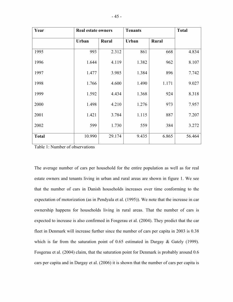
- 45 -

Year Real estate owners Tenants

Urban Rural Urban Rural

Total

1995

1996

1997

1998

1999

2000

2001

2002

993

1.644

1.477

1.766

1.592

1.498

1.421

599

2.312

4.119

3.985

4.600

4.434

4.210

3.784

1.730

861

1.382

1.384

1.490

1.368

1.276

1.115

559

668

962

896

1.171

924

973

887

384

4.834

8.107

7.742

9.027

8.318

7.957

7.207

3.272

Total 10.990 29.174 9.435 6.865 56.464

Table 1: Number of observations

The average number of cars per household for the entire population as well as for real

estate owners and tenants living in urban and rural areas are shown in figure 1. We see

that the number of cars in Danish households increases over time conforming to the

expectation of motorization (as in Pendyala et al. (1995)). We note that the increase in car

ownership happens for households living in rural areas. That the number of cars is

expected to increase is also confirmed in Fosgerau et al. (2004). They predict that the car

fleet in Denmark will increase further since the number of cars per capita in 2003 is 0.38

which is far from the saturation point of 0.65 estimated in Dargay & Gately (1999).

Fosgerau et al. (2004) claim, that the saturation point for Denmark is probably around 0.6

cars per capita and in Dargay et al. (2006) it is shown that the number of cars per capita is

- 46 -

lower in Denmark than in most other European countries14. We therefore do not expect

serious saturation effects to be present in Denmark.

0,00

0,20

0,40

0,60

0,80

1,00

1,20

1,40

1995 1996 1997 1998 1999 2000 2001 2002

Year

Ave

rage

num

ber o

f car

s pe

r hou

seho

ld

AllUrban real estate ownersRural real estate ownersUrban tenantsRural tenants

Figure 1: Car ownership for real estate owners and tenants in urban and rural areas.

Source: Danish Transport Diary Survey

The development in after-tax income for households is shown in figure 2 for real estate

owners and tenants living in urban and rural areas15. We see that not only do real estate

owning households have higher income than tenants. The income for real estate owners

also increases more than for tenants from 1995 to 2002, both in absolute terms and in

relative terms as shown in figure 3. A possible explanation for the increasing car

ownership seen in figure 1 is the increasing income shown in figure 2 since we expect

cars to be a normal good. One expectation emerging from figure 1 is that the income

14 Dargay et al. (2006) use data from EuroStat to show this. 15 We define urban areas as the five largest cities in Denmark (Copenhagen and suburbs, Århus, Odense, Ålborg and Esbjerg). Rural areas are defined as the remaining part of Denmark.

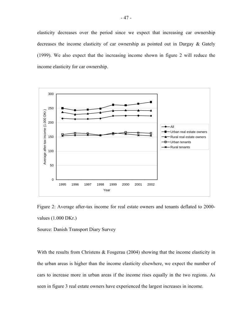
- 47 -

elasticity decreases over the period since we expect that increasing car ownership

decreases the income elasticity of car ownership as pointed out in Dargay & Gately

(1999). We also expect that the increasing income shown in figure 2 will reduce the

income elasticity for car ownership.

0

50

100

150

200

250

300

1995 1996 1997 1998 1999 2000 2001 2002

Year

Ave

rage

afte

r-tax

inco

me

(1.0

00 D

Kr.)

AllUrban real estate ownersRural real estate ownersUrban tenantsRural tenants

Figure 2: Average after-tax income for real estate owners and tenants deflated to 2000-

values (1.000 DKr.)

Source: Danish Transport Diary Survey

With the results from Christens & Fosgerau (2004) showing that the income elasticity in

the urban areas is higher than the income elasticity elsewhere, we expect the number of

cars to increase more in urban areas if the income rises equally in the two regions. As

seen in figure 3 real estate owners have experienced the largest increases in income.

- 48 -

90

92

94

96

98

100

102

104

106

108

110

1995 1996 1997 1998 1999 2000 2001 2002

Year

Inde

x fo

r afte

r-ta

x in

com

e (1

995=

100)

All

Urban real estate ow ners

Rural real estate ow ners

Urban tenants

Rural tenants

Figure 3: Index for after-tax income deflated to 2000 (1995=100)

Source: Danish Transport Diary Survey

Based on the increases in income we should expect car ownership to increase more for

households living in urban areas than elsewhere. But if we look at the regional

differences shown in figure 1 this is not the case. It turns out that it is the households not

living in the five largest cities who have experienced the largest increase in car ownership

even though their income has increased the least.

In this paper we speculate that the value of real estate influence the demand for cars. As

seen in Figure 4 the housing prices have increased significantly from 1992 to 2002 and if

the hypothesis that real estate values influence car demand is true a model not

incorporating this might produced biased forecasts.

- 49 -

0

200

400

600

800

1000

1200

1992 1993 1994 1995 1996 1997 1998 1999 2000 2001 2002

Average price

Apartments

One-familyhouses

Figure 4: Real estate prices (1.000 DKr.).

Source: Statistics Denmark.

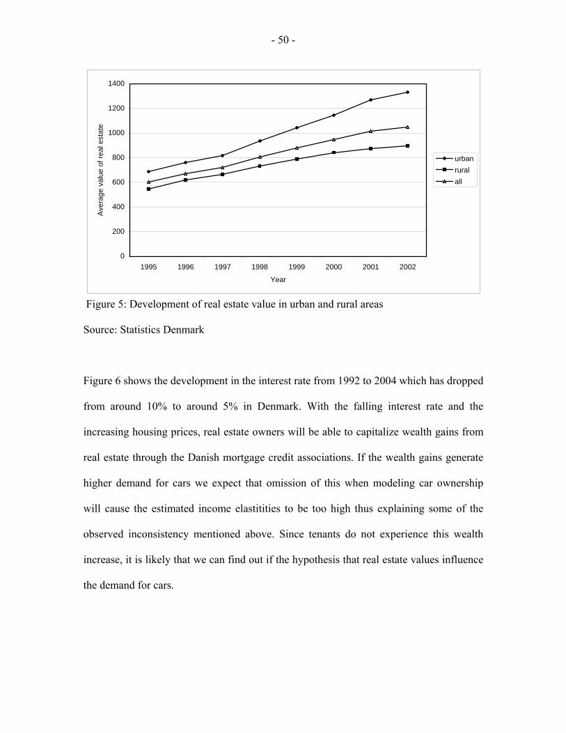
The developments in housing prices have differed much between rural and urban areas as

shown in figure 5. In 1995 the difference in average housing prices between urban and

rural areas was about 200.000 DKr. This difference increased to around 450.000 DKr.

and we thus see that urban households have gained much more wealth in housing than

rural households.

- 50 -

0

200

400

600

800

1000

1200

1400

1995 1996 1997 1998 1999 2000 2001 2002

Year

Ave

rage

val

ue o

f rea

l est

ate

urbanruralall

Figure 5: Development of real estate value in urban and rural areas

Source: Statistics Denmark

Figure 6 shows the development in the interest rate from 1992 to 2004 which has dropped

from around 10% to around 5% in Denmark. With the falling interest rate and the

increasing housing prices, real estate owners will be able to capitalize wealth gains from

real estate through the Danish mortgage credit associations. If the wealth gains generate

higher demand for cars we expect that omission of this when modeling car ownership

will cause the estimated income elastitities to be too high thus explaining some of the

observed inconsistency mentioned above. Since tenants do not experience this wealth

increase, it is likely that we can find out if the hypothesis that real estate values influence

the demand for cars.

- 51 -

With the changing housing prices being a flow variable we examine if the inclusion of a

variable for the value of real estate prices (a stock variable) influence real estate owners

and tenants differently. We obtain this variable from Statistics Denmark for every

municipality in Denmark and link it to the observations from the Danish Transport Diary

Survey. Ideally we should have the information for the individual observations but this

information is not available. We therefore assume that the average value of real estate in

the municipalities can be used as a proxy for the real estate value for households living in

that municipality.

0

2

4

6

8

10

12

1992 1993 1994 1995 1996 1997 1998 1999 2000 2001 2002 2003 2004

Figure 6: Interest on 30-years bonds.

Source: Statistics Denmark

- 52 -

To examine these things more closely, the next section sets up a multinomial logit model

for car ownership and estimated it on a series of neighboring cross-section data.

3. Model and estimation

The model used is a simple multinomial logit model16. With the choice variable for the

households being the number of cars this problem fits very well into a discrete

framework. The alternatives the households choose between are ‘no cars’, ‘one car’ or

‘more than one car’. Letting Y represent the number of cars chosen by the households,

and letting 0V , 1V , and 2V represent household utility when owning ‘no cars’, ‘one car’ or

‘more than one car’, and normalizing ‘no cars’ to zero we have the following standard

choice probabilities for the logit model

1 2

1

1 2

2

1 2

11

1

1

( 0)

( 1)

( 2)

V V

V

V V

V

V V

e e

ee e

ee e

P Y

P Y

P Y

+ +

+ +

+ +

= =

= =

≥ =

(1)

and the functions we estimate are

( 1)1 1( 0)

( 2)2 2( 0)

( ) log( )

( ) log( )

P YP Y

P YP Y

V X X

V X X

β

β

==

≥=

= =

= =

(2)

where 1β and 2β are vectors of parameters and X is a vector of observations. The

'sβ can now be found using standard maximum likelihood procedures. With the

specification given above we expect parameters that have a positive effect on car

16 For an introduction to the multinomial logit model see Ben-Akiva & Lerman (1985) or Train (2003)

- 53 -

ownership to fulfill 1 2β β< and parameters having a negative effect on car ownership to

fulfill 1 2β β> since the chosen specification sets parameters relative to having no car17.

As noted in Pendyala et al. (1995) it is important to account for differences in household

structure when it comes to the number of adults and children. We would like to estimate

separate models for different household types (couples with and without children, and

singles with and without children) but in order to keep the number of observations ‘high’

in every estimation, we instead include variables for the number of children under the age

of 16 and the number of people over the age of 16 in the household18. We expect both

variables to affect the probability of car ownership positively. Since the proximity (and

thus accessibility) of public transport also influences car ownership, we include a variable

for the distance between nearest public transport node and the home address and a

variable for the distance between nearest public transport node and the workplace. Our

expectation is that a longer distance to public transport increases the possibility of car

ownership. We also include a dummy variable for the degree of urbanization (e.g. living

in one of the 5 largest cities in Denmark or not) together with a variable for the age of the

interviewee since a higher degree of urbanization is expected to reduce the demand for

cars and people of different age have different demand for cars. We also include a

variable for age squared. Age is thus modeled in a polynomial way allowing us to capture

life-cycle effects. The income variable included accounts for total after-tax income in the

17 This point becomes clear if we had chosen

( 2)2 2( 1)( ) log( )P Y

P YV X Xβ≥== =

in which case 2β parameters are relative to having one car. 18 We would like the distinction to be at the age of 18 since this is the legal age in Denmark for acquiring a drivers license. But the data does not allow us to make this distinction.

- 54 -

households deflated to 2000 values. Furthermore we hypothesis, that households living in

areas where housing prices are ‘high’ might have a different demand for cars than

households living in areas where real estate values are ‘low’. We include a variable for

the average real estate value in the different municipalities. Since we do not have

information on individual wealth we will use this variable as a proxy for household

wealth. A list of all variables used in the model can be seen in table 2.

3.1 Estimating the model

The model is estimated allowing parameters to differ between years. We estimate the

model on the five different sets of data presented in table 1 and present the parameter

estimates and test statistics in table A.1 through A.5 in the appendix19. In general we find

that higher income gives a higher probability of car ownership and the signs of ‘Age’ and

‘Age2’ differ. We also see that poor access to public transport (e.g. longer distance from

home to nearest public transport node and longer distance from work to nearest public

transport node) gives a higher probability of car ownership. The composition of the

family also affects the choice probabilities as expected, since both the number of children

and the number of adults in the household has a positive effect on the choice

probabilities. Furthermore we see that people living in less urbanized areas have higher

probability of owning a car, and we find that not owning real estate gives a lower

19 The five sets are; urban real estate owners, rural real estate owners, urban tenants, rural tenants, and the entire sample.

- 55 -

probability of owning cars. All five models produce good values for the McFadden 2ρ

statistics20 between 0.34 and 0.43 which we find to be satisfactory.

Variable Description

Cars

Loginc

Age

Age2

Distpub

Workpub

Child

Adults

Urban

Owner

Value

Number of cars available to the household

Logaritm of household yearly after-tax income deflated to 2000 values

Age of the person interviewed

Squared value of age

Distance from home to public transport

Distance from workplace to public transport

Number of children younger than 16 in the household

Number of people not registered as children

Dummy for living in highly urbanized area (5 largest cities in Denmark)

Dummy for ownership of real estate (1 if real estate owner, 2 if tenant)

Average value of real estate in the municipality of residence

Table 2: Model variables

We also estimate models where we do not allow parameters to differ between years,

effectively pooling all observations together. Estimates and test statistics can also be

found in table A.1 through A.5 in the appendix. The signs are as expected and all five

models produce McFadden 2ρ statistics between 0.33 and 0.43 which we find to be

20 The McFadden 2ρ values are defined as ( )2

(0)(0) 1 LLβρ = − and ( )2

( )( ) 1 LL cc βρ = − where L(0), L(c) and L(β)

are likelihood values for estimations with zero coefficients, constants and all parameters respectively. A discussion of this measure can be found in Ortúzar & Willumsen (1994) chapter 8.

- 56 -

satisfactory. To examine if the restrictions on the parameters can be accepted we

calculate χ2-value in all five models for the restrictions that parameters are identical for

all years. The results are shown in table 3.

Likelihood of

unrestricted model

Likelihood of

restricted model

Degrees of

freedom

χ2-

value

A.1: All households

A.2: Urban owners

A.3: Rural owners

A.4: Urban tenants

A.5: Rural tenants

-37.021,3581

-7.953,7969

-18.055,3316

-5.846,9292

-4.752,4732

-37.305,5362

-8.060,4679

-18.176,7024

-5.970,4143

-4.817,3043

140

140

140

140

140

0,0000

0,0001

0,0000

0,0000

0,7236

Table 3: Test for restricting parameters

The restrictions in the full model (A.1) through (A.4) are strongly rejected but for tenants

living in rural areas the restriction is accepted. These households are also those which

should be affected the least, if the hypothesis that real estate values affect car demand is

correct since they do not own real estate and live in the areas which have experienced the

lowest increase in real estate values.

The difference between real estate owners and tenants in rural areas could indicate that

there is something causing parameter instability, which is not affecting tenants in rural

areas. To investigate further we examine if the inclusion of a variable for real estate

values change the results.

- 57 -

3.2 Estimating the model with a variable for real estate values

We now estimate the model where a variable for the real estate values are included. As

before we estimate both the restricted model where all parameters are identical for all

years and the unrestricted model where parameters are allowed to differ between years.

The results are shown in table A.6 through A.10 in the appendix. Table 4 summarizes the

statistics for the restrictions. As before we see that the restrictions are rejected in all cases

except for tenants living in rural areas. The next step is therefore to see if we can restrict

the parameter for real estate values to zero in any of the models used. This will be done

next.

Likelihood of

unrestricted

model

Likelihood of

restricted model

Degrees

of freedom

χ2-

value

A.6: All households

A.7: Urban owners

A.8: Rural owners

A.9: Urban tenants

A.10: Rural tenants

-36.916,0413

-7.841,0372

-18.041,8511

-5.819,2340

-4.744,1334

-37.247,5566

-8.001,3378

-18.172,5051

-5.961,9033

-4.815,1884

158

158

158

158

158

0,0000

0,0000

0,0000

0,0000

0,8127

Table 4: Test for restricting parameters in the models with a variable for real estate values

3.3 Testing for insignificant effect of real estate value

Table 5 and table 6 present the test results from testing the hypotheses that the variable

for real estate values can be set equal to zero. We test this both in the model with

different parameters for each year and in the model with identical parameters for all

years.

- 58 -

Likelihood of

unrestricted model

Likelihood of

restricted model

Degrees

of freedom

χ2-

value

A.6: All households (βvalue=0)

A.7: Urban owners (βvalue=0)

A.8: Rural owners (βvalue=0)

A.9: Urban tenants (βvalue=0)

A.10: Rural tenants (βvalue=0)

-36.916,0413

-7.841,0372

-18.041,8511

-5.819,2340

-4.744,1334

--37.021,3581

-7.953,7969

-18.055,3316

-5.846,9292

-4.752,4732

20

20

20

20

20

0,0000

0,0000

0,1364

0,0000

0,6737

Table 5: Test for restricting parameters in the models with a variable for real estate values

The results of this test are clear. For households living in rural areas the restriction is

accepted and we conclude that the real estate values have not significantly affected these

households. For urban areas the restriction is not accepted. We believe that this indicates

that our hypothesis that real estate values affect car demand could be correct. As we saw

in figure 6 the largest increases in real estate values have happened in urban areas and the

assumption of no influence of the real estate values are rejected for households living

here.

Likelihood of

unrestricted model

Likelihood of

restricted model

Degrees

of freedom

χ2-

value

A.6: All households (βvalue=0)

A.7: Urban owners (βvalue=0)

A.8: Rural owners (βvalue=0)

A.9: Urban tenants (βvalue=0)

A.10: Rural tenants (βvalue=0)

-37.247,5566

-8.001,3378

-18.172,5051

-5.961,9033

-4.815,1884

-37.305,5362

-8.060,4679

-18.176,7024

-5.970,4143

-4.817,3043

6

6

6

6

6

0,0000

0,0000

0,2106

0,0092

0,6453

Table 6: Test for restricting parameters in the models with a variable for real estate values

and identical parameters for all years

- 59 -

4. Calculating income elasticities

We now use the unrestricted models to find income elasticities for car ownership for the

different household groups. These can be found by using the model to simulate the

changing choice probabilities when the income changes. We first calculate income

elasticities using the model without a variable for real estate values but with separate

parameters for all years. The results are shown in figure 7.

0

0,2

0,4

0,6

0,8

1

1,2

1,4

1995 1996 1997 1998 1999 2000 2001 2002

Year

Inco

me

elas

ticity

for c

ar o

wne

rshi

p

All households

Owners inurban areas

Owners in ruralareas

Tenants inurban areas

Tenants in ruralareas

Figure 7: Income elasticities for car ownership (not including a variable for real estate

values)

It is clear that in general tenants have higher income elasticities than real estate owners

and urban households have higher income elasticities than rural households. We also see

that the conventional wisdom that the income elasticity for car ownership should fall over

- 60 -

time is not rejected in our model. Looking at figure 7 it also becomes clear that income

elasticities are not stable.

The magnitude of the elasticities found for all households are higher than those reported

in Birkeland et al. (2000) but in line with those reported by Dargay (2001) using a

pseudo-panel analysis. The findings also conform to the differences in income elasticities

between urban and rural households reported in Christens & Fosgerau (2004) and the size

of the elasticities found here are in line with their findings.

One explanation for the difference in income elasticity between real estate owners and

tenants could be that real estate owners have higher car ownership than tenants as shown

in figure 1, which reduces the income elasticity for car ownership for real estate owners.

Furthermore, real estate owners in general have higher income than tenants which also

cause tenants to have higher income elasticities for car ownership than real estate owners.

Now we calculate elasticities using the model where real estate values are included. The

results can be seen in figure 8. The same picture as before arises with urban households

having higher income elasticities than rural households and with tenants having higher

income elasticities than real estate owners. Comparing figure 7 and figure 8 we see that

the inclusion of a variable for real estate values have decreased the elasticities for all

households with the largest decrease for real estate owners. We take this as an indication

that the real estate values have biased the income elasticities upwards. Calculating the

best-fit straight lines for the development in income elasticities shown in figure 7 and

- 61 -

figure 8 we can make a comparison of the slopes and the constants to see how the

estimates are affected by the inclusion of the variable for real estate value. These are

shown in table 8.

0

0,2

0,4

0,6

0,8

1

1,2

1,4

1995 1996 1997 1998 1999 2000 2001 2002

Year

Inco

me

elas

ticity

for c

ar o

wne

rshi

p

All households

Ow ners in urban areas

Ow ners in rural areas

Tenants in urban areas

Tenants in rural areas

Figure 8: Income elasticities for car ownership (including a variable for real estate

values)

It is clear that the inclusion of the variable for real estate values have reduced the slope

numerically and the constants for the straight line equations shown. As we see the largest

changes have happened for real estate owners with a slope for urban real estate owners

increasing from -0.0302 to -0.0212 and for rural real estate owners the slope increased

from -0.0185 to -0.0110. This is an increase of 0.0090 and 0.0075. For tenants the

increases in the slope have only been 0.0025 and 0.0002. It is thus clear that the largest

- 62 -

impact of including the variable for real estate values have been in the elasticities for real

estate owners.

For real estate owners the change in the slope due to the inclusion of a variable for real

estate value is 29.8% for urban real estate owners and 40.5% for rural real estate owners.

For tenants the change in slope is 17.5% for urban tenants and 1.0% for rural tenants. For

the model with all households the change is 15.1%.

For real estate owners the change in constant due to the inclusion of a variable for real

estate value is 14.7% for urban real estate owners and 24.9% for rural real estate owners.

For tenants the change in constant is 2.3% for urban tenants and 0.8% for rural tenants.

For the model with all households the change is 5.4%. We conclude that the real estate

values influence real estate owners and tenants differently and we see that omission of a

variable for real estate prices have biased the income elastities upwards. Further

examination of this topic we address in Nielsen (2006).

Without real estate values With real estate values

All households 0.6813-0.0185*year 0.6443-0.0157*year

Urban owners 0.8165-0.0302*year 0.6962-0.0212*year

Rural owners 0.6813-0.0185*year 0.5116-0.0110*year

Urban tenants 1.1969-0.0143*year 1.1692-0.0118*year

Rural tenants 0.9110-0.0192*year 0.9036-0.0190*year

Table 7: Best-fit linear equations for income elasticities

(year=0 for 1995, year=1 for 1996,…, year=7 for 2002)

- 63 -

5. Conclusion

In this paper we addressed the problem of bias in estimated parameters when simple

cross-section methods are used to determine car ownership. The problem of parameter

instability is not unknown and ideally time series should be used. Unfortunately transport

researchers are often forced to use simple methods due to data limitations. Identification

of variables which can reduce the problem is therefore in demand. We used repeated

cross-section analysis of Danish data to show that the omission of a variable for real

estate values bias estimated income elastities upwards. By dividing data into four groups

which we expect to be affected differently by real estate values we are able to analyze the

hypothesis that real estate values influence car demand. We showed that the inclusion of

a variable for real estate values in the Danish municipalities reduce the estimated income

elasticities showing us that omission of this variable cause the estimates to be upward

biased.

- 64 -

References

Ben-Akiva, M. & Lerman, S. R. (1985) Discrete Choice Analysis: Theory and

Application to Travel Demand, The MIT Press, Cambridge, England.

Birkeland, M. E., Brems, C. R. and Kabelmann, T. (2000) Analyse af personers

transportarbejde, 1975-1998, Trafikdage på Aalborg Universitet 2000, Conference paper

(www.trafikdage.dk)

Bjørner, T. B. (1999) Estimation af elasticiteter for persontransporten med bil, in

Transport Demand and Environmental Regulation in the Transport Sector, Ph.D.

dissertation, Rød Serie 54, Department of Economics, University of Copenhagen.

Christens, P. F. & Fosgerau, M. (2004) Rådighed over bil, En beskrivelse af

sammenhængen mellem husstandsindkomst, bilrådighed og geografi, Notat 3:2004,

Danish Transport Research Institute.

Dargay, J. M. and Gately, D. (1999) Income’s effect on car and vehicle ownership,

worldwide: 1960-2015, Transportation Research Part A, 33, 101-138.

Dargay, J. M and Vythoulkas, P. C. (1999) Estimation of a Dynamic Car Ownership

Model: A Pseudo-panel Approach, Journal of Transport Economics and Policy 33:3, 287-

302.

Dargay, J. M. (2001) The effect of income on car ownership: evidence and asymmetry,

Transportation Research Part A 35, 807-821.

Dargay, J. M. (2002) Determinants of car ownership in rural and urban areas: a pseudo-

panel analysis, Transportation Research Part E, 38, 351-366.

Dargay, J., Hivert, L. and Legros, D. (2006) The dynamics of car ownership in E.U

countries: a comparison based on the european household panel survey, working paper.

- 65 -

Deaton, A. (1985) Panel Data from Time Series of Cross Sections, Journal of

Econometrics 30, 109-126.

De Jong, G., Pieters, M., Miller, S., Daly, A., Plasmeijer, R., Graafland, I., Lierens, A.,

Baak, J., Walker, W. & Kroes, E. (2005), Uncertainty in traffic Forecasts – Literature

Review and New Results for the Netherlands, Rand Europe for the AVV Transport

Research Centre.

Fosgerau, M., Holmblad, M. & Pilegaard, N. (2004) ART – En aggregeret

prognosemodel for dansk vejtrafik, Notat 5:2004, Danish Transport Research Institute.

Jansson, J. O. (1989) Car demand modeling and forecasting – A New Approach, Journal

of Transport Economics and Policy 13:2, 125-140.

Kwon, T. and Preston, J. (2005) Driving Forces behind the Growth of Per-capita Car

Driving Distance in the UK, 1970-2000, Transport Reviews 25:4, 467-490.

Nielsen, J. E. (2006a) Real estate ownership and the demand for cars in Denmark – A

pseudo-panel analysis, Thesis paper.

Nielsen, J. E. (2006b) Demand for car transport in Denmark – Differences between rural

and urban households, Thesis paper.

Orhúzar, J. de D. and Willumsen, L. G. (1994) Modelling Transport, Second Edition,

John Wiley & Sons, Chichester.

Oum, T. H., Waters II, W. G. & Yong, J-S. (1992) Concepts of price elasticities of

transport demand and recent empirical estimates, An Interpretative Survey, Journal of

Transport Economics and Policy 26:2, 139-154.

Pendyala, R. M., Kostyniuk, L. P. & Goulias, K. G. (1995) A repeated cross-sectional

evaluation of car ownership, Transportation 22, 165-184.

- 66 -

Train, K. (1980) A Structured Logit Model of Auto Ownership and Mode Choice, The

Review of Economic Studies 47:2, 357-370.

Train, K. E. (2003) Discrete Choice Methods with Simulation, Cambridge University

Press, Cambridge, United Kingdom.

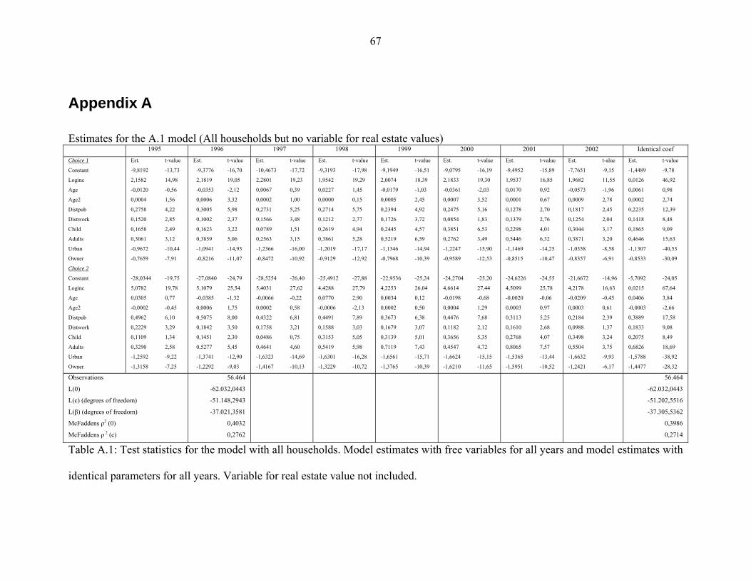
67

Appendix A

Estimates for the A.1 model (All households but no variable for real estate values) 1995 1996 1997 1998 1999 2000 2001 2002 Identical coef

Choice 1

Constant

Loginc

Age

Age2

Distpub

Distwork

Child

Adults

Urban

Owner

Choice 2

Constant

Loginc

Age

Age2

Distpub

Distwork

Child

Adults

Urban

Owner

Est. t-value

-9,8192 -13,73

2,1582 14,98

-0,0120 -0,56

0,0004 1,56

0,2758 4,22

0,1520 2,85

0,1658 2,49

0,3061 3,12

-0,9672 -10,44

-0,7659 -7,91

-28,0344 -19,75

5,0782 19,78

0,0305 0,77

-0,0002 -0,45

0,4962 6,10

0,2229 3,29

0,1109 1,34

0,3290 2,58

-1,2592 -9,22

-1,3158 -7,25

Est. t-value

-9,3776 -16,70

2,1819 19,05

-0,0353 -2,12

0,0006 3,32

0,3005 5,98

0,1002 2,37

0,1623 3,22

0,3859 5,06

-1,0941 -14,93

-0,8216 -11,07

-27,0840 -24,79

5,1079 25,54

-0,0385 -1,32

0,0006 1,75

0,5075 8,00

0,1842 3,50

0,1451 2,30

0,5277 5,45

-1,3741 -12,90

-1,2292 -9,03

Est. t-value

-10,4673 -17,72

2,2801 19,23

0,0067 0,39

0,0002 1,00

0,2731 5,25

0,1566 3,48

0,0789 1,51

0,2563 3,15

-1,2366 -16,00

-0,8472 -10,92

-28,5254 -26,40

5,4031 27,62

-0,0066 -0,22

0,0002 0,58

0,4322 6,81

0,1758 3,21

0,0486 0,75

0,4641 4,60

-1,6323 -14,69

-1,4167 -10,13

Est. t-value

-9,3193 -17,98

1,9542 19,29

0,0227 1,45

0,0000 0,15

0,2714 5,75

0,1212 2,77

0,2619 4,94

0,3861 5,28

-1,2019 -17,17

-0,9129 -12,92

-25,4912 -27,88

4,4288 27,79

0,0770 2,90

-0,0006 -2,13

0,4491 7,89

0,1588 3,03

0,3153 5,05

0,5419 5,98

-1,6301 -16,28

-1,3229 -10,72

Est. t-value

-9,1949 -16,51

2,0074 18,39

-0,0179 -1,03

0,0005 2,45

0,2394 4,92

0,1726 3,72

0,2445 4,57

0,5219 6,59

-1,1346 -14,94

-0,7968 -10,39

-22,9536 -25,24

4,2253 26,04

0,0034 0,12

0,0002 0,50

0,3673 6,38

0,1679 3,07

0,3139 5,01

0,7119 7,43

-1,6561 -15,71

-1,3765 -10,39

Est. t-value

-9,0795 -16,19

2,1833 19,30

-0,0361 -2,03

0,0007 3,52

0,2475 5,16

0,0854 1,83

0,3851 6,53

0,2762 3,49

-1,2247 -15,90

-0,9589 -12,53

-24,2704 -25,20

4,6614 27,44

-0,0198 -0,68

0,0004 1,29

0,4476 7,68

0,1182 2,12

0,3656 5,35

0,4547 4,72

-1,6624 -15,15

-1,6210 -11,65

Est. t-value

-9,4952 -15,89

1,9537 16,85

0,0170 0,92

0,0001 0,67

0,1278 2,70

0,1379 2,76

0,2298 4,01

0,5446 6,32

-1,1469 -14,25

-0,8515 -10,47

-24,6226 -24,55

4,5099 25,78

-0,0020 -0,06

0,0003 0,97

0,3113 5,25

0,1610 2,68

0,2768 4,07

0,8065 7,57

-1,5365 -13,44

-1,5951 -10,52

Est. t-alue

-7,7651 -9,15

1,9682 11,55

-0,0573 -1,96

0,0009 2,78

0,1817 2,45

0,1254 2,04

0,3044 3,17

0,3871 3,20

-1,0358 -8,58

-0,8357 -6,91

-21,6672 -14,96

4,2178 16,63

-0,0209 -0,45

0,0003 0,61

0,2184 2,39

0,0988 1,37

0,3498 3,24

0,5504 3,75

-1,6632 -9,93

-1,2421 -6,17

Est. t-value

-1,4489 -9,78

0,0126 46,92

0,0061 0,98

0,0002 2,74

0,2235 12,39

0,1418 8,48

0,1865 9,09

0,4646 15,63

-1,1307 -40,53

-0,8533 -30,09

-5,7092 -24,05

0,0215 67,64

0,0406 3,84

-0,0003 -2,66

0,3889 17,58

0,1833 9,08

0,2075 8,49

0,6826 18,69

-1,5788 -38,92

-1,4477 -28,32

Observations

L(0)

L(c) (degrees of freedom)

L(β) (degrees of freedom)

McFaddens ρ2 (0)

McFaddens ρ 2 (c)

56.464

-62.032,0443

-51.148,2943

-37.021,3581

0,4032

0,2762

56.464

-62.032,0443

-51.202,5516

-37.305,5362

0,3986

0,2714

Table A.1: Test statistics for the model with all households. Model estimates with free variables for all years and model estimates with

identical parameters for all years. Variable for real estate value not included.

68

Estimates for the A.2 model (Urban real estate owners but no variable for real estate values) 1995 1996 1997 1998 1999 2000 2001 2002 Identical coef

Choice 1

Constant

Loginc

Age

Age2

Distpub

Distwork

Child

Adults

Choice 2

Constant

Loginc

Age

Age2

Distpub

Distwork

Child

Adults

Est. t-value

-13,1682 -8,34

2,0563 6,49

0,0400 0,77

-0,0001 -0,14

0,2759 1,66

0,2773 2,02

0,2177 1,59

0,6365 2,99

-33,3122 -11,00

5,3125 9,71

0,0471 0,57

-0,0001 -0,14

0,2945 1,42

0,3885 2,24

0,0841 0,49

0,6676 2,54

Est. t-value

-13,6167 -11,70

2,3969 10,03

0,0142 0,38

0,0002 0,58

0,1637 1,23

0,0703 0,75

0,2445 2,24

0,3190 2,16

-35,7628 -14,32

5,5732 12,83

0,0936 1,38

-0,0005 -0,69

0,4651 2,79

0,1750 1,44

0,4020 2,99

0,3990 2,08

Est. t-value

-14,3422 -11,48

2,4116 9,09

0,0461 1,20

-0,0002 -0,42

0,4930 3,48

0,1738 1,57

-0,0307 -0,30

0,1179 0,71

-37,0878 -15,52

5,7955 13,76

0,1156 1,69

-0,0009 -1,21

0,9114 5,09

0,0633 0,45

0,0381 0,29

0,2587 1,20

Est. t-value

-11,1457 -10,81

1,7169 8,21

0,0143 0,38

0,0003 0,68

0,5187 3,71

0,0158 0,16

0,4233 3,79

0,5894 3,89

-28,3874 -15,30

4,2024 13,27

0,0982 1,65

-0,0007 -1,13

0,8760 5,27

-0,1435 -1,11

0,4529 3,42

0,5831 3,01

Est. t-value

-11,2608 -10,04

1,9496 8,35

-0,0326 -0,79

0,0008 1,82

0,3257 2,35

0,1573 1,42

0,4610 4,01

0,4921 2,99

-27,4226 -14,06

4,3128 12,66

-0,0270 -0,41

0,0008 1,08

0,6585 3,95

0,0599 0,43

0,5414 3,92

0,8643 4,22

Est. t-value

-11,5683 -10,58

1,9376 8,18

0,0059 0,14

0,0004 0,87

0,3652 2,69

-0,0789 -0,72

0,4563 3,89

0,3312 2,04

-26,1558 -13,82

4,3841 12,98

-0,0571 -0,88

0,0010 1,47

0,6468 3,92

-0,1129 -0,80

0,5696 4,12

0,5114 2,49

Est. t-value

-13,8841 -10,87

2,3117 8,99

0,0039 0,09

0,0005 1,09

0,5027 3,29

0,1299 1,13

0,3348 2,77

0,2887 1,68

-29,6404 -14,62

4,6372 13,15

0,0026 0,04

0,0006 0,85

0,5969 3,16

0,0404 0,28

0,4664 3,24

0,7404 3,50

Est. t-value

-7,6215 -4,13

1,7115 4,42

-0,1535 -1,95

0,0023 2,71

0,0697 0,28

0,1646 1,11

0,7590 3,76

0,4379 1,56

-22,1481 -7,33

3,9633 7,26

-0,1243 -1,13

0,0020 1,70

0,0447 0,15

0,0434 0,24

0,7461 3,25

0,4582 1,35

Est. t-value

-4,1225 -13,64

0,0112 22,56

0,0191 1,32

0,0002 1,37

0,3568 6,89

0,1003 2,58

0,2901 6,80

0,4290 7,05

-9,6952 -19,38

0,0188 32,70

0,0719 3,04

-0,0004 -1,44

0,6128 9,68

0,0753 1,52

0,3689 7,20

0,6566 8,67

Observations

L(0)

L(c) (degrees of freedom)

L(β) (degrees of freedom)

McFaddens ρ 2 (0)

McFaddens ρ 2 (c)

10.990

-12.073,7491

-10.125,5609

-7.953,7969

0,3412

0.2145

10.990

-12.073,7491

-10.132,4230

-8.060,4679

0,3324

0,2025

Table A.2: Test statistics for the model with all households. Model estimates with free variables for all years and model estimates with

identical parameters for all years. Variable for real estate value not included.

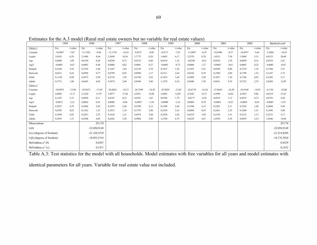
69

Estimates for the A.3 model (Rural real estate owners but no variable for real estate values) 1995 1996 1997 1998 1999 2000 2001 2002 Identical coef

Choice 1

Constant

Loginc

Age

Age2

Distpub

Distwork

Child

Adults

Choice 2

Constant

Loginc

Age

Age2

Distpub

Distwork

Child

Adults

Est. t-value

-10,9887 -7,07

2,0183 6,29

0,0488 1,09

-0,0003 -0,67

0,3246 2,92

0,0231 0,24

0,1130 0,98

0,3731 1,80

-30,4935 -13,98

4,8902 11,71

0,1455 2,33

-0,0015 -2,21

0,5927 4,79

0,0705 0,65

0,1098 0,85

0,3053 1,33

Est. t-value

-11,7382 -9,46

2,1496 8,64

0,0150 0,44

0,0002 0,48

0,2782 3,48

0,0598 0,77

0,3072 2,99

0,6665 4,03

-29,9672 -17,69

5,1220 15,79

0,0050 0,11

0,0002 0,43

0,4586 5,03

0,1262 1,47

0,2851 2,55

0,8388 4,65

Est. t-value

-13,1728 -10,24

2,5698 10,36

0,0269 0,73

0,0000 0,02

0,1467 1,84

0,0799 0,93

0,2138 1,95

0,3874 2,40

-30,4862 -18,13

5,4977 17,48

0,0107 0,22

0,0000 -0,06

0,2555 2,86

0,1015 1,10

0,1434 1,21

0,6262 3,58

Est. t-value

-9,8357 -8,98

1,7775 8,28

0,0135 0,40

0,0001 0,37

0,2154 2,70

0,0990 1,17

0,4746 3,83

0,8548 5,48

-26,7399 -18,59

4,2921 16,06

0,0781 1,82

-0,0007 -1,44

0,3599 4,13

0,1793 2,00

0,4974 3,84

0,9908 5,90

Est. t-value

-8,9171 -7,55

1,4695 6,17

0,0418 1,16

-0,0003 -0,73

0,1015 1,42

0,2311 2,64

0,1853 1,66

1,1276 6,34

-22,9029 -15,85

3,6003 12,89

0,0786 1,79

-0,0008 -1,63

0,1949 2,48

0,2258 2,43

0,2638 2,26

1,2704 6,75

Est. t-value

-11,0497 -8,35

2,2570 8,70

-0,0249 -0,61

0,0006 1,37

0,1855 2,41

0,0344 0,39

0,4989 3,49

0,6890 3,70

-26,8778 -16,54

4,7645 15,57

-0,0177 -0,36

0,0004 0,70

0,3540 4,15

0,0896 0,95

0,4519 3,05

0,9229 4,67

Est. t-value

-10,9490 -8,37

1,8521 7,54

0,0554 1,39

-0,0003 -0,61

0,0290 0,40

0,1980 2,00

0,1857 1,59

0,8621 4,76

-27,0654 -16,50

4,3990 14,82

0,0555 1,12

-0,0003 -0,52

0,2201 2,71

0,2461 2,35

0,2354 1,91

1,0530 5,38

Est. t-value

-10,4957 -5,66

1,9860 5,31

0,0099 0,16

0,0002 0,25

0,1578 1,35

0,1799 1,53

0,1766 0,92

0,7323 2,76

-25,9104 -10,93

4,3955 9,86

0,0555 0,72

-0,0005 -0,65

0,1938 1,48

0,1880 1,51

0,2332 1,17

0,9039 3,19

Est. t-value

-3,2004 -10,43

0,0123 20,40

0,0354 2,65

-0,0001 -0,92

0,1560 5,51

0,1187 3,75

0,2202 5,17

0,8204 12,99

-8,1781 -22,00

0,0218 33,81

0,0756 4,46

-0,0007 -3,95

0,3004 9,49

0,1696 5,00

0,2333 5,17

1,0106 14,88

Observations

L(0)

L(c) (degrees of freedom)

L(β) (degrees of freedom)

McFaddens ρ2 (0)

McFaddens ρ 2 (c)

29.174

-32.050,9149

-21.168,3518

-18.055,3316

0,4367

0,1471

29.174

-32.050,9149

-21.214,8269

-18.176,7024

0,4329

0,1432

Table A.3: Test statistics for the model with all households. Model estimates with free variables for all years and model estimates with

identical parameters for all years. Variable for real estate value not included.

70

Estimates for the A.4 model (Urban tenants but no variable for real estate values) 1995 1996 1997 1998 1999 2000 2001 2002 Identical coef

Choice 1

Constant

Loginc

Age

Age2

Distpub

Distwork

Child

Adults

Choice 2

Constant

Loginc

Age

Age2

Distpub

Distwork

Child

Adults

Est. t-value

-12,2322 -10,41

2,3956 9,02

-0,0374 -0,92

0,0006 1,42

0,1851 1,16

-0,0400 -0,36

0,3117 2,16

0,0444 0,23

-31,2998 -5,81

5,1608 5,07

-0,1269 -0,80

0,0015 0,79

0,6917 1,56

-0,0523 -0,18

0,0372 0,10

1,3582 2,83

Est. t-value

-10,6336 -12,00

2,3504 11,42

-0,1226 -3,98

0,0015 4,53

0,2597 2,23

0,1106 1,24

0,1467 1,46

0,1299 0,95

-25,1345 -8,47

4,3206 7,36

-0,0169 -0,19

0,0000 -0,02

0,8821 3,48

0,0547 0,27

-1,0878 -2,89

-0,1297 -0,38

Est. t-value

-11,1991 -12,22

2,0526 10,13

-0,0385 -1,24

0,0006 1,88

0,3032 2,57

0,1640 1,84

0,0608 0,58

0,2638 1,75

-31,9303 -7,75

6,2462 8,25

-0,3122 -2,77

0,0038 2,96

-0,3416 -0,65

0,8800 3,84

-0,0008 0,00

0,3345 0,71

Est. t-value

-13,2917 -14,29

2,1779 11,29

0,0486 1,65

-0,0002 -0,73

0,3145 2,88

0,1760 1,90

0,1145 1,15

-0,0510 -0,37

-31,8202 -9,55

4,7447 7,81

0,0978 0,98

-0,0007 -0,63

0,7034 2,56

0,0148 0,06

-0,4361 -1,40

0,2844 0,83

Est. t-value

-12,4605 -13,24

2,4414 12,11

-0,0594 -1,83

0,0009 2,50

0,3266 2,75

0,1054 0,98

0,3775 3,75

0,0614 0,44

-25,3325 -8,87

4,1904 7,95

-0,0430 -0,46

0,0005 0,51

0,6219 2,22

0,1995 0,91

0,1634 0,73

0,3734 1,20

Est. t-value

-11,5224 -12,32

2,2995 11,59

-0,0739 -2,24

0,0010 2,84

0,4141 3,49

0,1499 1,51

0,3894 3,61

-0,0330 -0,24

-34,3646 -8,83

5,8738 8,21

-0,0034 -0,03

0,0004 0,33

0,5858 1,80

0,2807 1,16

-0,1225 -0,42

-0,8083 -1,81

Est. t-value

-10,8954 -11,49

1,8349 8,90

0,0111 0,31

0,0001 0,20

0,0196 0,17

-0,0543 -0,47

0,1621 1,46

0,5333 3,22

-28,3631 -7,88

4,9150 7,99

-0,1193 -0,99

0,0013 0,92

0,4236 1,17

-0,1235 -0,45

0,0924 0,35

0,8046 1,82

Est. t-value

-11,5442 -8,00

2,1013 6,69

-0,0164 -0,32

0,0003 0,62

0,3781 2,06

-0,0808 -0,62

0,4882 2,39

0,2304 1,02

-26,5916 -5,60

4,6859 5,19

-0,1610 -1,04

0,0016 0,92

0,5089 1,11

-0,0061 -0,02

0,3657 1,06

1,2380 2,34

Est. t-value

-3,3886 -14,00

0,0132 27,77

-0,0146 -1,26

0,0004 3,06

0,2467 5,78

0,1016 2,85

0,2039 5,11

0,2057 3,77

-8,5283 -11,48

0,0230 26,33

-0,0345 -0,92

0,0005 1,15

0,5314 4,69

0,2122 2,51

-0,1700 -1,68

0,4200 3,34

Observations

L(0)

L(c) (degrees of freedom)

L(β) (degrees of freedom)

McFaddens ρ 2 (0)

McFaddens ρ 2 (c)

9.435

-10.365,4069

-7.498,6473

-5.846,9292

0,4359

0,2203

9.435

-10.365,4069

-7.507,2105

-5.970,4143

0,4240

0,2047

Table A.4: Test statistics for the model with all households. Model estimates with free variables for all years and model estimates with

identical parameters for all years. Variable for real estate value not included.

71

Estimates for the A.5 model (Rural tenants but no variable for real estate values) 1995 1996 1997 1998 1999 2000 2001 2002 Identical coef

Choice 1

Constant

Loginc

Age

Age2

Distpub

Distwork

Child

Adults

Choice 2

Constant

Loginc

Age

Age2

Distpub

Distwork

Child

Adults

Est. t-value

-10,0490 -7,92

2,1192 7,48

-0,0599 -1,46

0,0008 1,81

0,2676 2,25

0,3073 3,12

0,1056 0,67

0,1007 0,49

-26,9017 -6,78

4,8788 6,29

-0,0758 -0,64

0,0008 0,58

0,3811 1,61

0,4244 2,45

-0,4890 -1,42

0,2602 0,62

Est. t-value

-10,1520 -9,17

1,8542 7,24

0,0090 0,26

-0,0001 -0,16

0,3893 3,83

0,1394 1,70

0,0120 0,12

0,3518 1,89

-29,3039 -8,40

5,2491 7,65

-0,1189 -1,13

0,0011 0,83

0,5859 3,20

0,4122 2,79

0,1172 0,59

0,8120 2,19

Est. t-value

-11,8626 -9,69

2,2532 8,66

0,0037 0,10

0,0002 0,48

0,3192 3,15

0,1781 2,13

0,0666 0,57

0,0479 0,26

-31,9003 -9,31

5,3295 8,52

0,0576 0,60

-0,0006 -0,56

0,6851 4,31

0,1770 1,25

-0,0095 -0,05

0,1878 0,57

Est. t-value

-10,3137 -10,53

2,0324 9,48

0,0011 0,04

0,0001 0,19

0,2271 2,78

0,1273 1,57

0,1311 1,22

0,1383 0,88

-24,8556 -10,12

4,1739 8,83

-0,0252 -0,36

0,0003 0,43

0,3934 2,90

0,1206 0,90

0,4296 2,76

0,7768 2,92

Est. t-value

-9,5764 -8,51

1,9026 7,91

-0,0419 -1,20

0,0006 1,52

0,3271 3,37

0,1289 1,55

-0,0573 -0,52

0,4525 2,51

-29,5413 -9,09

5,1596 8,32

-0,0602 -0,63

0,0007 0,63

0,5505 3,44

0,2631 1,79

0,0062 0,03

0,5170 1,41

Est. t-value

-9,4138 -8,80

1,9314 8,29

-0,0418 -1,28

0,0006 1,64

0,1734 2,03

0,1930 2,25

0,2366 1,98

0,2306 1,40

-26,0697 -8,59

3,8689 7,56

0,1432 1,43

-0,0018 -1,47

0,5809 3,85

0,0186 0,12

0,1732 0,90

0,3890 1,49

Est. t-value

-10,4882 -9,20

1,9687 7,91

-0,0009 -0,03

0,0002 0,56

0,1507 1,70

0,2131 2,45

0,2639 2,24

0,2331 1,30

-29,4290 -8,43

5,0107 7,74

-0,0109 -0,09

0,0001 0,04

0,3607 1,92

0,0345 0,18

-0,0618 -0,25

0,6504 1,85

Est. t-value

-7,6365 -4,98

2,0162 5,83

-0,1094 -1,93

0,0012 1,95

0,0728 0,56

0,2315 1,87

-0,0462 -0,24

0,0892 0,39

-19,7749 -5,18

3,2026 4,69

0,0949 0,70

-0,0012 -0,81

0,2568 1,20

-0,1136 -0,52

0,1053 0,38

0,1280 0,33

Est. t-value

-2,7396 -10,57

0,0147 21,97

-0,0060 -0,49

0,0002 1,43

0,2281 6,80

0,1870 6,07

0,0782 1,84

0,2150 3,33

-8,3348 -13,19

0,0250 24,64

0,0115 0,34

-0,0002 -0,53

0,4625 7,90

0,1959 3,59

0,1085 1,52

0,5763 5,13

Observations

L(0)

L(c) (degrees of freedom)

L(β) (degrees of freedom)

McFaddens ρ 2 (0)

McFaddens ρ 2 (c)

6.865

-7.541,9734

-5.919,4227

-4.752,4732

0,3699

0,1971

6.865

-7.541,9734

-5.926,5814

-4.817,3043

0,3613

0,1872

Table A.5: Test statistics for the model with all households. Model estimates with free variables for all years and model estimates with

identical parameters for all years. Variable for real estate value not included.

72

Estimates for the A.6 model (All households and a variable for real estate values) 1995 1996 1997 1998 1999 2000 2001 2002 Identical coef

Choice 1

Constant

Loginc

Age

Age2

Distpub

Distwork

Child

Adults

Urban

Owner

Value

Choice 2

Constant

Loginc

Age

Age2

Distpub

Distwork

Child

Adults

Urban

Owner

Value

Est. t-value

-10,1048 -14,02

2,1139 14,62

-0,0116 -0,54

0,0004 1,50

0,2676 4,10

0,1531 2,87

0,1494 2,23

0,2996 3,03

-1,0744 -10,90

-0,6464 -6,27

0,0008 3,36

-28,1495 -19,74

4,8584 18,75

0,0337 0,85

-0,0003 -0,61

0,4906 6,02

0,2248 3,31

0,0796 0,96

0,3358 2,62

-1,6364 -10,65

-1,0061 -5,31

0,0017 5,69

Est. t-value

-9,7002 -17,18

2,1105 18,31

-0,0374 -2,24

0,0006 3,33

0,2884 5,75

0,1001 2,37

0,1368 2,70

0,3904 5,08

-1,2346 -15,86

-0,6379 -7,93

0,0010 5,81

-27,1152 -24,72

4,8732 24,07

-0,0419 -1,43

0,0006 1,74

0,4953 7,81

0,1911 3,62

0,1106 1,74

0,5467 5,60

-1,7261 -14,58

-0,8678 -6,02

0,0017 7,72

Est. t-value

-10,5801 -17,90

2,2282 18,69

0,0043 0,25

0,0002 1,05

0,2646 5,09

0,1560 3,47

0,0622 1,19

0,2644 3,24

-1,3258 -16,20

-0,7336 -8,74

0,0005 3,49

-28,5041 -26,34

5,2782 26,61

-0,0090 -0,30

0,0002 0,58

0,4277 6,74

0,1757 3,21

0,0249 0,39

0,4793 4,74

-1,8145 -14,87

-1,2266 -8,32

0,0008 4,12

Est. t-value

-9,5156 -18,26

1,9021 18,66

0,0192 1,22

0,0000 0,26

0,2614 5,55

0,1203 2,75

0,2410 4,53

0,3837 5,23

-1,3241 -17,63

-0,7758 -10,21

0,0006 4,76

-25,3696 -27,64

4,2330 26,11

0,0739 2,78

-0,0006 -2,15

0,4410 7,76

0,1614 3,08

0,2841 4,52

0,5544 6,10

-1,9381 -17,25

-1,0658 -8,24

0,0011 6,59

Est. t-value

-9,3042 -16,68

1,9585 17,81

-0,0195 -1,12

0,0005 2,47

0,2363 4,87

0,1721 3,72

0,2331 4,34

0,5249 6,61

-1,2407 -14,92

-0,7029 -8,60

0,0004 3,27

-22,9351 -25,19

4,0972 24,88

0,0021 0,08

0,0001 0,47

0,3709 6,45

0,1704 3,12

0,2962 4,71

0,7199 7,49

-1,8896 -15,83

-1,2038 -8,72

0,0007 4,40

Est. t-value

-9,1202 -16,26

2,1624 18,95

-0,0368 -2,07

0,0007 3,54

0,2447 5,10

0,0876 1,87

0,3803 6,43

0,2776 3,50

-1,2712 -14,98

-0,9214 -11,35

0,0002 1,37

-24,1350 -25,00

4,5572 26,34

-0,0200 -0,69

0,0004 1,25

0,4488 7,70

0,1245 2,23

0,3539 5,16

0,4633 4,80

-1,8263 -14,75

-1,5156 -10,52

0,0004 2,72

Est. t-value

-9,5093 -15,90

1,9512 16,69

0,0167 0,90

0,0001 0,68

0,1268 2,68

0,1380 2,76

0,2290 3,99

0,5442 6,31

-1,1568 -12,62

-0,8437 -9,81

0,0000 0,30

-24,3291 -24,20

4,3540 24,52

-0,0007 -0,02

0,0003 0,84

0,3243 5,47

0,1635 2,72

0,2638 3,87

0,8182 7,67

-1,7865 -13,47

-1,4529 -9,28

0,0004 3,23

Est. t-value

-7,8113 -9,18

1,9555 11,40

-0,0575 -1,97

0,0009 2,78

0,1816 2,45

0,1252 2,04

0,3019 3,14

0,3907 3,23

-1,0807 -7,69

-0,8100 -6,36

0,0001 0,65

-21,5514 -14,85

4,1333 16,04

-0,0207 -0,44

0,0003 0,58

0,2220 2,44

0,0992 1,38

0,3475 3,22

0,5576 3,80

-1,8220 -9,29

-1,1642 -5,60

0,0003 1,49

Est. t-value

-1,6420 -10,84

0,0124 45,79

0,0054 0,86

0,0002 2,75

0,2200 12,20

0,1433 8,56

0,1805 8,79

0,4709 15,79

-1,1916 -39,96

-0,7972 -26,75

0,0003 6,11

-6,1339 -25,41

0,0209 64,75

0,0404 3,81

-0,0003 -2,84

0,3899 17,63

0,1874 9,28

0,1934 7,90

0,6992 19,10

-1,7655 -39,78

-1,3107 -24,89

0,0006 10,46

Observations

L(0)

L(c) (degrees of freedom)

L(β) (degrees of freedom)

McFaddens ρ2 (0)

McFaddens ρ 2 (c)

56.464

-62.032,0443

-51.148,2943 (18)

-36.916,0413 (180)

0,4049

0,2783

56.464

-62.032,0443

-51.202,5516 (2)

-37.247,5566 (22)

0,3995

0,2725

Table A.6: Test statistics for the model with all households. Model estimates with free variables for all years and model estimates with

identical parameters for all years. Variable for real estate value included.

73

Estimates for the A.7 model (Urban real estate owners and a variable for real estate values)

1995 1996 1997 1998 1999 2000 2001 2002 Identical coef

Choice 1

Constant

Loginc

Age

Age2

Distpub

Distwork

Child

Adults

Value

Choice 2

Constant

Loginc

Age

Age2

Distpub

Distwork

Child

Adults

Value

Est. t-value

-12,7202 -8,07

1,8781 5,78

0,0397 0,76

-0,0001 -0,24

0,2460 1,47

0,2891 2,09

0,1611 1,16

0,6070 2,81

0,0010 2,35

-31,7394 -10,38

4,7132 8,47

0,0571 0,68

-0,0004 -0,40

0,2122 1,01

0,4121 2,34

-0,0351 -0,20

0,6661 2,50

0,0023 4,58

Est. t-value

-12,5693 -10,77

2,1086 8,63

-0,0065 -0,17

0,0003 0,79

0,0432 0,32

0,0969 1,02

0,1365 1,23

0,2806 1,87

0,0018 5,84

-33,3613 -13,18

4,9049 11,05

0,0706 1,02

-0,0005 -0,62

0,2974 1,74

0,2095 1,69

0,2662 1,94

0,3906 2,00

0,0027 7,40

Est. t-value

-13,6642 -10,91

2,2103 8,17

0,0425 1,10

-0,0002 -0,50

0,4349 3,06

0,1746 1,57

-0,0946 -0,90

0,1348 0,80

0,0008 3,13

-35,8590 -14,89

5,4350 12,58

0,1141 1,67

-0,0010 -1,33

0,8499 4,74

0,0577 0,41

-0,0501 -0,37

0,2881 1,32

0,0011 3,56

Est. t-value

-10,8348 -10,50

1,6197 7,66

0,0054 0,15

0,0003 0,72

0,4442 3,16

0,0161 0,16

0,3318 2,90

0,5412 3,54

0,0008 3,63

-26,4259 -14,08

3,6939 11,33

0,0888 1,48

-0,0008 -1,19

0,7808 4,67

-0,1489 -1,14

0,2985 2,19

0,5600 2,87

0,0014 5,72

Est. t-value

-10,8919 -9,69

1,7949 7,62

-0,0458 -1,10

0,0009 1,91

0,2835 2,03

0,1680 1,51

0,3733 3,19

0,4289 2,60

0,0010 4,52

-25,4350 -12,91

3,7540 10,72

-0,0459 -0,69

0,0008 1,12

0,6092 3,63

0,1033 0,74

0,3884 2,74

0,7781 3,76

0,0018 6,58

Est. t-value

-11,3777 -10,41

1,8342 7,66

0,0006 0,01

0,0004 0,86

0,2985 2,18

-0,0568 -0,52

0,3945 3,30

0,3061 1,88

0,0006 2,98

-25,0223 -13,11

4,0567 11,72

-0,0680 -1,04

0,0010 1,46

0,5699 3,43

-0,0743 -0,53

0,4601 3,25

0,4984 2,42

0,0010 4,14

Est. t-value

-13,7924 -10,78

2,2742 8,77

0,0005 0,01

0,0005 1,11

0,4888 3,21

0,1229 1,07

0,3191 2,62

0,2778 1,62

0,0002 1,18

-28,3596 -13,89

4,2597 11,83

0,0041 0,06

0,0005 0,67

0,5613 2,96

0,0167 0,11

0,4031 2,77

0,7385 3,48

0,0008 3,55

Est. t-value

-7,4517 -4,03

1,6152 4,13

-0,1591 -2,03

0,0024 2,75

0,0251 0,10

0,1785 1,20

0,7310 3,62

0,4481 1,58

0,0004 1,43

-21,4223 -7,05

3,7243 6,71

-0,1333 -1,20

0,0021 1,73

-0,0080 -0,03

0,0544 0,30

0,7278 3,16

0,4689 1,37

0,0006 1,93

Est. t-value

-4,3066 -14,17

0,0107 20,96

0,0166 1,14

0,0002 1,23

0,3235 6,25

0,1083 2,77

0,2530 5,88

0,4297 7,02

0,0005 6,74

-10,0625 -19,94

0,0173 29,37

0,0699 2,94

-0,0004 -1,73

0,5701 8,98

0,0864 1,73

0,2955 5,69

0,6690 8,79

0,0009 10,51

Observations

L(0)

L(c) (degrees of freedom)

L(β) (degrees of freedom)

McFaddens ρ 2 (0)

McFaddens ρ 2 (c)

10.990

-12.073,7491

-10.125,5609 (18)

-7.841,0372 (180)

0,3506

0,2256

10.990

-12.073,7491

-10.132,4230 (2)

-8.001,3378 (22)

0,3373

0,2103

Table A.7: Test statistics for the model with all households. Model estimates with free variables for all years and model estimates with

identical parameters for all years. Variable for real estate value included.

74

Estimates for the A.8 model (Rural real estate owners and a variable for real estate values)

1995 1996 1997 1998 1999 2000 2001 2002 Identical coef

Choice 1

Constant

Loginc

Age

Age2

Distpub

Distwork

Child

Adults

Value

Choice 2

Constant

Loginc

Age

Age2

Distpub

Distwork

Child

Adults

Value

Est. t-value

-10,9842 -7,06

2,0336 6,25

0,0488 1,09

-0,0003 -0,66

0,3238 2,91

0,0235 0,24

0,1146 0,99

0,3727 1,79

-0,0002 -0,28

-30,4213 -13,94

4,8057 11,36

0,1470 2,36

-0,0016 -2,25

0,6017 4,86

0,0686 0,63

0,1068 0,83

0,3142 1,36

0,0006 0,93

Est. t-value

-11,7386 -9,44

2,2000 8,73

0,0164 0,48

0,0002 0,47

0,2770 3,46

0,0603 0,77

0,3185 3,08

0,6626 4,00

-0,0005 -1,37

-29,8701 -17,61

5,1189 15,56

0,0060 0,13

0,0002 0,43

0,4607 5,04

0,1298 1,51

0,2951 2,62

0,8391 4,65

-0,0002 -0,50

Est. t-value

-13,2030 -10,27

2,5037 9,99

0,0237 0,64

0,0000 0,07

0,1497 1,88

0,0861 1,00

0,2017 1,84

0,4003 2,47

0,0007 1,80

-30,5557 -18,16

5,4559 17,09

0,0076 0,16

0,0000 -0,03

0,2554 2,86

0,1070 1,16

0,1327 1,12

0,6364 3,63

0,0006 1,31

Est. t-value

-9,8478 -8,98

1,7687 8,16

0,0134 0,40

0,0001 0,37

0,2163 2,72

0,0991 1,17

0,4739 3,83

0,8541 5,48

0,0001 0,29

-26,7402 -18,57

4,2738 15,78

0,0780 1,82

-0,0007 -1,44

0,3616 4,15

0,1797 2,00

0,4969 3,84

0,9915 5,90

0,0001 0,39

Est. t-value

-8,9202 -7,55

1,4820 6,12

0,0418 1,16

-0,0003 -0,72

0,1014 1,42

0,2310 2,64

0,1864 1,67

1,1242 6,32

-0,0001 -0,29

-22,9384 -15,86

3,6475 12,84

0,0785 1,78

-0,0008 -1,61

0,1889 2,40

0,2245 2,42

0,2657 2,27

1,2632 6,71

-0,0003 -0,85

Est. t-value

-11,0389 -8,35

2,2960 8,69

-0,0261 -0,64

0,0006 1,40

0,1822 2,36

0,0356 0,40

0,5014 3,50

0,6826 3,67

-0,0002 -0,78

-26,8801 -16,53

4,8116 15,41

-0,0190 -0,39

0,0004 0,74

0,3498 4,09

0,0904 0,96

0,4544 3,07

0,9155 4,64

-0,0002 -0,81

Est. t-value

-11,0392 -8,42

1,9819 7,88

0,0604 1,51

-0,0003 -0,69

0,0192 0,27

0,1885 1,88

0,1973 1,67

0,8417 4,63

-0,0007 -2,98

-27,0133 -16,45

4,4498 14,68

0,0606 1,22

-0,0003 -0,61

0,2236 2,73

0,2389 2,25

0,2442 1,96

1,0424 5,31

-0,0005 -1,66

Est. t-value

-10,4784 -5,64

2,0136 5,33

0,0100 0,16

0,0002 0,26

0,1526 1,30

0,1816 1,55

0,1792 0,93

0,7277 2,74

-0,0002 -0,56

-25,8419 -10,88

4,3957 9,71

0,0563 0,72

-0,0005 -0,65

0,1914 1,45

0,1901 1,53

0,2359 1,18

0,9014 3,18

-0,0001 -0,27

Est. t-value

-3,1744 -10,21

0,0124 20,22

0,0355 2,66

-0,0001 -0,92

0,1554 5,48

0,1186 3,75

0,2207 5,18

0,8191 12,96

0,0000 -0,48

-8,2534 -21,90

0,0217 33,16

0,0759 4,48

-0,0007 -3,98

0,3039 9,59

0,1706 5,03

0,2326 5,16

1,0146 14,92

0,0001 0,99

Observations

L(0)

L(c) (degrees of freedom)

L(β) (degrees of freedom)

McFaddens ρ2 (0)

McFaddens ρ 2 (c)

29.174

-32.050,9149

-21.168,3518 (18)

-18.041,8511 (180)

0,4371

0,1477

29.174

-32.050,9149

-21.214,8269 (2)

-18.172,5051 (22)

0,4330

0,1434

Table A.8: Test statistics for the model with all households. Model estimates with free variables for all years and model estimates with

identical parameters for all years. Variable for real estate value included.

75

Estimates for the A.9 model (Urban tenants and a variable for real estate values)

1995 1996 1997 1998 1999 2000 2001 2002 Identical

coef

Choice 1

Constant

Loginc

Age

Age2

Distpub

Distwork

Child

Adults

Value

Choice 2

Constant

Loginc

Age

Age2

Distpub

Distwork

Child

Adults

Value

Est. t-value

-10,9842 -7,06

2,0336 6,25

0,0488 1,09

-0,0003 -0,66

0,3238 2,91

0,0235 0,24

0,1146 0,99

0,3727 1,79

-0,0002 -0,28

-30,4213 -13,94

4,8057 11,36

0,1470 2,36

-0,0016 -2,25

0,6017 4,86

0,0686 0,63

0,1068 0,83

0,3142 1,36

0,0006 0,93

Est. t-value

-11,7386 -9,44

2,2000 8,73

0,0164 0,48

0,0002 0,47

0,2770 3,46

0,0603 0,77

0,3185 3,08

0,6626 4,00

-0,0005 -1,37

-29,8701 -17,61

5,1189 15,56

0,0060 0,13

0,0002 0,43

0,4607 5,04

0,1298 1,51

0,2951 2,62

0,8391 4,65

-0,0002 -0,50

Est. t-value

-13,2030 -10,27

2,5037 9,99

0,0237 0,64

0,0000 0,07

0,1497 1,88

0,0861 1,00

0,2017 1,84

0,4003 2,47

0,0007 1,80

-30,5557 -18,16

5,4559 17,09

0,0076 0,16

0,0000 -0,03

0,2554 2,86

0,1070 1,16

0,1327 1,12

0,6364 3,63

0,0006 1,31

Est. t-value

-9,8478 -8,98

1,7687 8,16

0,0134 0,40

0,0001 0,37

0,2163 2,72

0,0991 1,17

0,4739 3,83

0,8541 5,48

0,0001 0,29

-26,7402 -18,57

4,2738 15,78

0,0780 1,82

-0,0007 -1,44

0,3616 4,15

0,1797 2,00

0,4969 3,84

0,9915 5,90

0,0001 0,39

Est. t-value

-8,9202 -7,55

1,4820 6,12

0,0418 1,16

-0,0003 -0,72

0,1014 1,42

0,2310 2,64

0,1864 1,67

1,1242 6,32

-0,0001 -0,29

-22,9384 -15,86

3,6475 12,84

0,0785 1,78

-0,0008 -1,61

0,1889 2,40

0,2245 2,42

0,2657 2,27

1,2632 6,71

-0,0003 -0,85

Est. t-value

-11,0389 -8,35

2,2960 8,69

-0,0261 -0,64

0,0006 1,40

0,1822 2,36

0,0356 0,40

0,5014 3,50

0,6826 3,67

-0,0002 -0,78

-26,8801 -16,53

4,8116 15,41

-0,0190 -0,39

0,0004 0,74

0,3498 4,09

0,0904 0,96

0,4544 3,07

0,9155 4,64

-0,0002 -0,81

Est. t-value

-11,0392 -8,42

1,9819 7,88

0,0604 1,51

-0,0003 -0,69

0,0192 0,27

0,1885 1,88

0,1973 1,67

0,8417 4,63

-0,0007 -2,98

-27,0133 -16,45

4,4498 14,68

0,0606 1,22

-0,0003 -0,61

0,2236 2,73

0,2389 2,25

0,2442 1,96

1,0424 5,31

-0,0005 -1,66

Est. t-value

-10,4784 -5,64

2,0136 5,33

0,0100 0,16

0,0002 0,26

0,1526 1,30

0,1816 1,55

0,1792 0,93

0,7277 2,74

-0,0002 -0,56

-25,8419 -10,88

4,3957 9,71

0,0563 0,72

-0,0005 -0,65

0,1914 1,45

0,1901 1,53

0,2359 1,18

0,9014 3,18

-0,0001 -0,27

Est. t-value

-3,4162 -13,69

0,0132 27,66

-0,0145 -1,26

0,0004 3,05

0,2464 5,77

0,1016 2,85

0,2041 5,12

0,2078 3,80

0,0000 0,38

-8,8793 -11,84

0,0224 25,34

-0,0404 -1,08

0,0005 1,26

0,5054 4,45

0,2289 2,70

-0,1778 -1,74

0,4472 3,55

0,0008 4,09

Observations

L(0)

L(c) (degrees of freedom)

L(β) (degrees of freedom)

McFaddens ρ 2 (0)

McFaddens ρ 2 (c)

9.435

-10.365,4069

-7.498,6473 (18)

-5.819,2340 (180)

0,4386

0,2240

9.435

-10.365,4069

-7.507,2105 (2)

-5.961,9033 (22)

0,4248

0,2058

Table A.9: Test statistics for the model with all households. Model estimates with free variables for all years and model estimates with

identical parameters for all years. Variable for real estate value included.

76

Estimates for the A.10 model (Rural tenants and a variable for real estate values)

1995 1996 1997 1998 1999 2000 2001 2002 Identical

coef

Choice 1

Constant

Loginc

Age

Age2

Distpub

Distwork

Child

Adults

Value

Choice 2

Constant

Loginc

Age

Age2

Distpub

Distwork

Child

Adults

Value

Est. t-value

-10,2408 -8,03

2,1066 7,45

-0,0606 -1,48

0,0008 1,82

0,2685 2,24

0,3061 3,11

0,0918 0,58

0,0939 0,46

0,0007 1,51

-27,2850 -6,78

4,9552 6,26

-0,0723 -0,61

0,0008 0,54

0,3798 1,59

0,4148 2,39

-0,4906 -1,41

0,2553 0,61

-0,0001 -0,11

Est. t-value

-10,3889 -9,28

1,8258 7,10

0,0120 0,35

-0,0001 -0,24

0,3840 3,77

0,1464 1,79

-0,0013 -0,01

0,3578 1,91

0,0007 1,92

-29,3952 -8,43

5,1725 7,46

-0,1172 -1,11

0,0010 0,81

0,5752 3,13

0,4199 2,83

0,1011 0,50

0,8317 2,24

0,0010 1,30

Est. t-value

-11,8521 -9,69

2,2284 8,54

0,0010 0,03

0,0002 0,55

0,3208 3,15

0,1815 2,17

0,0631 0,54

0,0419 0,23

0,0004 0,97

-31,9786 -9,24

5,3275 8,39

0,0574 0,59

-0,0006 -0,55

0,6890 4,31

0,1785 1,26

-0,0137 -0,07

0,1806 0,55

0,0002 0,29

Est. t-value

-10,3785 -10,57

2,0232 9,42

-0,0010 -0,03

0,0001 0,26

0,2255 2,75

0,1286 1,59

0,1225 1,14

0,1396 0,88

0,0003 0,94

-24,5007 -10,02

4,0545 8,53

-0,0385 -0,55

0,0005 0,59

0,3753 2,76

0,1375 1,01

0,3979 2,54

0,7853 2,96

0,0010 1,76

Est. t-value

-9,6147 -8,54

1,8866 7,82

-0,0432 -1,23

0,0006 1,56

0,3283 3,38

0,1273 1,53

-0,0653 -0,59

0,4507 2,50

0,0003 0,82

-29,5657 -9,10

5,1346 8,22

-0,0614 -0,64

0,0007 0,64

0,5517 3,45

0,2626 1,79

-0,0039 -0,02

0,5172 1,41

0,0003 0,52

Est. t-value

-9,4050 -8,78

1,9434 8,30

-0,0403 -1,23

0,0006 1,59

0,1750 2,05

0,1897 2,20

0,2409 2,02

0,2298 1,39

-0,0002 -0,65

-26,0277 -8,56

3,8679 7,51

0,1429 1,42

-0,0018 -1,46

0,5834 3,86

0,0191 0,12

0,1716 0,88

0,3868 1,48

0,0000 -0,08

Est. t-value

-10,6433 -9,28

1,9550 7,83

-0,0036 -0,10

0,0002 0,63

0,1532 1,72

0,2231 2,55

0,2570 2,20

0,2062 1,14

0,0005 1,77

-29,5114 -8,43

4,9587 7,57

-0,0123 -0,11

0,0001 0,04

0,3655 1,94

0,0500 0,26

-0,0714 -0,29

0,6269 1,78

0,0007 1,06

Est. t-value

-7,5970 -4,94

2,0198 5,84

-0,1084 -1,91

0,0012 1,93

0,0735 0,57

0,2319 1,87

-0,0411 -0,22

0,0947 0,41

-0,0001 -0,39

-19,8121 -5,16

3,1782 4,63

0,0908 0,67

-0,0012 -0,79

0,2422 1,12

-0,1170 -0,53

0,0809 0,29

0,0953 0,24

0,0005 0,80

Est. t-value

-2,8064 -10,71

0,0147 21,81

-0,0072 -0,59

0,0002 1,51

0,2273 6,77

0,1886 6,12

0,0745 1,76

0,2142 3,31

0,0002 1,80

-8,4312 -13,29

0,0248 24,26

0,0086 0,25

-0,0002 -0,47

0,4606 7,87

0,2003 3,66

0,1006 1,40

0,5752 5,12

0,0004 1,67

Observations

L(0)

L(c) (degrees of freedom)

L(β) (degrees of freedom)

McFaddens ρ 2 (0)

McFaddens ρ 2 (c)

6.865

-7.541,9734

-5.919,4227 (18)

-4.744,1334 (180)

0,3710

0,1985

6.865

-7.541,9734

-5.926,5814 (2)

-4.815,1884 (22)

0,3615

0,1875

Table A.10: Test statistics for the model with all households. Model estimates with free variables for all years and model estimates

with identical parameters for all years. Variable for real estate value included.

77

Real estate ownership and the demand for cars in

Denmark

- A pseudo-panel analysis

Jens Erik Nielsen

Danish Transport Research Institute

and

University of Copenhagen

Abstract

This paper examines how real estate ownership, increasing real estate values and the

falling interest rates affect car demand. It uses data from the Danish Transport Diary

Survey together with data from Statistics Denmark to estimate a simple partial adjustment

model for car ownership in Danish households. We find that car ownership differs among

households owning real estate and households not owning real estate and we find that real

estate owners have increased their demand for cars as a result of the increasing real estate

values and that other households are unaffected by the increasing real estate values.

Furthermore we show that both household groups have increased their demand for cars

due to the falling interest rate. We also find that long-run income elasticities for car

ownership differ between rural and urban households.

78

1. Introduction

The modeling and forecasting of car ownership is often based on cross section data in a

discrete model setting (e.g. logit or probit) where it is assumed that the parameters

estimated remain constant over time. There are two underlying assumptions behind this.

The first is that that the economy is in equilibrium. The other is that observed differences

in consumption between, e.g., a high income person and a low income person is a valid

description of what would happen if a low income person suddenly received the same

income as the high income person, all other things being equal. Both these assumptions

are probably invalid. What is needed is a dynamic model which explicitly takes account

of the dynamic nature of car demand.

Ideally, panel data should be used but since these are rarely available in the transport

sector and since many cross section data exist, the simpler approach of cross-section

modeling is often adopted and it is argued that the elasticities found are long-run

elasticities21. Deaton (1985) shows that it is possible to create panel data from repeated

cross-section data named pseudo-panel data. He shows that by using a characteristic that

is invariant over time for a given household type (e.g. year of birth of the oldest person in

the household) it is possible to create a pseudo panel describing average behavior for the

household type in question. The use of pseudo-panel data is an attempt to circumvent

some of the shortcomings of the cross-sectional data and use the strength of the time

series analysis. The pseudo panel approach also allows for the inclusion of macro

21 In Goodwin et. al. (2004) a survey of many recent elasticity studies are presented and a discussion of the claim that the elasticities found in simple cross-section studies can be interpreted as long-run elasticities can also be found here.

79

variables which might affect both the transport behavior (e.g. number of kilometers

traveled) and the demand for transport vehicles (e.g. cars). This paper utilizes the Danish

Transport Diary Survey together with data from Statistics Denmark to create a pseudo-

panel data set for the Danish population based on the year of birth for the interviewee in

the Danish Transport Diary Survey, real estate ownership status for the interviewees

household, and whether the household lives in an urban or rural area. It examines how

changing real estate values and a falling interest rate affect the number of cars available

in Danish households and to what extent the different types of households differ with

regard to income elasticities. To our knowledge this is the first time the effect of the

development in real estate prices and the interest rate is linked to the demand for cars.

The approach suggested by Deaton has been utilized in a number of papers. An

estimation of dynamic car ownership models is undertaken for the first time in Dargay

and Vythoulkas (1999) where the UK Family Expenditure Survey is used. They

demonstrate that the pseudo-panel method can be applied and gives credible estimates

when it comes to describing the dynamics of transport behavior. They also show that

there are large differences between short and long run elasticities with the latter being

three times bigger than the former. Birkeland et al. (2000) use data from the Danish

Tranport Diary Survey in a pseudo panel analysis of personal transport in Denmark. They

use a non-dynamic model to identify cohort effects and life-cycle effects. They also

compare income elasticities estimated by simple cross-section analysis with those found

by the use of pseudo panel data, showing that the two approaches yield very different

results. They conclude that pseudo panel methods are preferable when predicting future

80

demand for transport. In another paper (Nielsen (2006b)) we use repeated cross-section

analysis to investigate the demand for cars in Denmark and we show that housing prices

probably influence the demand for cars. The present paper is thus a continuation of the

work in Nielsen (2006b). In Dargay (2001) a pseudo-panel for UK is constructed and the

approach is used to show that hysteresis effects are present for car ownership. She shows

that the elasticities with regard to rising income is higher than the elasticities for falling

income. This hysteresis shows that a car after it is purchased becomes a necessity, which

is not disposed of as easily as it is acquired. Using the same data as in Dargay (2001) the

approach is later used in Dargay (2002) to show that important differences in the

elasticities between rural and urban households exists and that rural households have

lower income elasticities than urban households.

In Denmark the real estate values have increased steadily and at very high rates since

1993 and at the same time the long run interest rate has dropped from around 10% to

around 5%. This is shown in figure 1 and figure 2.

In a situation like the one experienced in Denmark with ricing real estate prices and

falling interest rate, households already owning real estate can (after a few years)

withdraw equity from their real estate without increasing monthly mortgage payments

due to the fall in the long run interest rate. Such an increase in wealth could increase the

number of cars in households. For households entering the real estate market the effect is

less clear. The fact that the real estate value increases will make it more expensive to

purchase a house or an apartment and the mortgage payments will be higher than for

81

those households who already own real estate. The decreasing interest rate will counter

this by reducing the mortgage payments. If the first effect dominates the households will

have less income available for consumption which will reduce the number of cars. If the

latter effect dominates the mortgage payments will go down and the household will have

more income available for consumption which could increase the number of cars in the

households.

0

200

400

600

800

1000

1200

1992 1993 1994 1995 1996 1997 1998 1999 2000 2001 2002

Prices onapartments

Prices onone-familyhouses

Figure 1: Real estate prices (1.000 DKr.).

Source: Statistics Denmark

Since the interest rate is the same for all households in the country we examine real estate

owners and tenants separately. This enables us to see if the changing real estate prices

and the changing interest rate has affected the two groups differently. Our expectation is

82

that the falling interest rate could affect both groups but the increasing real estate values

only affect the real estate owners. One problem is that the interest rate and the housing

prices are correlated and that non-real estate owners may face different credit market

constraints than real estate owners. If these capital restrictions for non-real estate owners

are strong we expect that the interest rate has affected the real estate owners more and

may even have had no effect on non real estate owners.

0

2

4

6

8

10

12

1992 1993 1994 1995 1996 1997 1998 1999 2000 2001 2002 2003 2004

Figure 2: Interest on 30-years bonds.

Source: Statistics Denmark

This paper extends the findings in previous studies by looking at the differences between

real estate owners and tenants, thus providing more insight into the behavior of different

83

household groups. It also identify effects of rising real estate prices and falling interest

rates on car demand which is new to the transport literature. Furthermore, we also

identify differences between urban and rural households, showing that these groups have

different long run income elasticities but fairly identical short run income elasticities with

regard to car ownership. The findings show that rural households have lower long run

elasticities and thus that they adjust their vehicle stock more slowly than urban

households, supporting findings for the UK in Dargay (2002).

The paper proceeds as follows. Section 2 discusses the data and the construction of the

pseudo-panel. Section 3 sets up the model and section 4 presents the estimations. Section

5 calculates different elasticities and discusses the results. Section 6 concludes.

2. The pseudo-panel data

The data utilized in the present paper come from two sources, the Danish Transport Diary

Survey and Statistics Denmark. The people participating in the Danish Transport Diary

Survey are selected by random draw from the Danish Civil Register. Data concerning the

individual as well as the household are collected and the travel pattern for a single day for

the interviewee is recorded. In the years 1992 to 1997 a monthly sample of 1800 was

drawn for people between the age of 16 and 74. In 1998 this was extended to 2100 and

the age group was extended to 10 to 84. The response rate in the survey is about 65-70%.

The variables included in the present analysis are after-tax income, number of adult

household members, degree of urbanization (living in a major Danish city or not), car

availability (how many cars the household has access to), information about whether the

household owns real estate, and if they live in a house or in an apartment. Due to data

84

limitations on certain variables, the sample used here is restricted to the years 1996 to

2002.

The pseudo panel is constructed by dividing the data into cohorts. Following Deaton

(1985) the cohorts have to be based on some characteristic that remain invariant in the

period analyzed. In the present study we have used the year of birth of the interviewee as

the determining factor together with real-estate ownership status and degree of

urbanization. The two latter may not be invariant over time but in this study we exclude

moving patterns thus assuming that households do not change residence. We thus assume

that real-estate ownership status and the degree of urbanization remains invariant over

time for all households. Each of the cohorts’ averages for all the variables included are

then calculated resulting in a ‘representative’ observation for the given cohort which in

our panel is an interviewee born in a given year, who is either a real estate owners or a

tenant, and either lives in an urban or rural area. This means that for a representative

person born in e.g. 1945 or in 1960, who is a tenant in an urban area we have a series of

observations from 1996 to 2002 describing the behavior of the representative person each

year. This data can then be linked to the macro data for the development in housing prices

and interest rate obtained from Statistics Denmark giving us the pseudo panel used in the

paper.

Car ownership includes both ownership of cars and other cars which the household can

use for personal transport22. Car ownership is calculated as the total number of cars

22 The appropriate expression would be ‘car availability’ since the respondents are asked if they have access to a car.

85

available to the households divided by the number of households for every cohort year.

These are shown in figure 3 and figure 4 where the car ownership for different cohorts

over time according to age is shown. Figure 3 shows the cohorts for real estate owners

and figure 4 shows the cohorts for tenants. It is clear from these figures that there is a

huge difference not only between households living in cities and on the countryside but

also between real estate owners and tenants.

Figure 3: Car ownership by cohort for real estate owners.

Source: Danish Transport Diary Survey.

86

The figures show that the life-cycle effect is larger for real estate owners. It is also clear

that households living in less urbanized areas have higher car ownership than households

living in large cities or in Copenhagen. One explanation of this is that the public transport

network is better and distances are smaller in cities, thus reducing the need for a car23.

Figure 4: Car ownership by cohort for tenants.

Source: Danish Transport Diary Survey.

Figure 5 gives another picture of a life cycle effect for households. It depicts the number

of adults living in a household. As the age of the interviewee increases, the number of

23 See Nielsen (2006a) for further discussion.

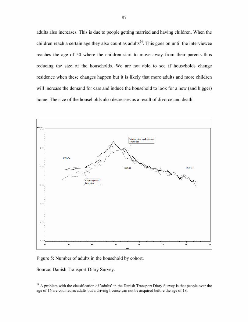
87

adults also increases. This is due to people getting married and having children. When the

children reach a certain age they also count as adults24. This goes on until the interviewee

reaches the age of 50 where the children start to move away from their parents thus

reducing the size of the households. We are not able to see if households change

residence when these changes happen but it is likely that more adults and more children

will increase the demand for cars and induce the household to look for a new (and bigger)

home. The size of the households also decreases as a result of divorce and death.

Figure 5: Number of adults in the household by cohort.

Source: Danish Transport Diary Survey.

24 A problem with the classification of ’adults’ in the Danish Transport Diary Survey is that people over the age of 16 are counted as adults but a driving license can not be acquired before the age of 18.

88

Figure 6: Average real estate values for cohorts (real estate owners).

Source: Statistics Denmark.

Unfortunately the Danish Transport diary Survey does not include information

concerning the value of real estate owned by the households. Data for the average

housing prices in the separate municipalities can be obtained from Statistics Denmark and

these data can be linked to the information in the Danish Transport diary Survey for each

household living in a given municipality. We thus assume that these average values are

the same for each household in a given municipality25. It is well known that the

development in housing prices has differed significantly between different regions in

25 We are also able to distinguish between households living in apartments and households living in houses. This is important since the development in market values for these two types of housing differs.

89

Denmark, with the largest increases happening in the greater Copenhagen area and the

large cities. This can be seen in figure 6 where the average real estate values for different

cohorts are shown. Furthermore it seems that for urban households the older cohorts have

experienced higher increases than younger cohorts and in rural areas the picture is the

opposite with the oldest cohorts having experienced the lowest increases in real estate

values.

The interest rate shown in figure 2 is also obtained from Statistics Denmark on an annual

basis. Since this is a general macro variable, all households in the economy face the same

interest rate. Some households might have limited access to the financial market, but we

ignore this and assume that all households have the same opportunities for borrowing

money and that they all face the same long run interest rate26.

As mentioned earlier it would be preferable to use real panel data but using a pseudo-

panel also hold some advantages. One advantage is that we do not need to include the

same households in each observation. The problem of finding a panel and following the

same panel over a long period is thus avoided. A tradeoff has to be made between the

number of individuals in a given cohort and the number of cohorts constructed. In our

case we have 11 cohorts, 2 degrees of urbanization, and 2 states for real estate ownership.

In all we therefore have 44 observations which we track over a period of 7 years. It is also

clear that when using a pseudo-panel we loose information about the variation between

the individuals within a given cohort. If the variation is large one could argue that the loss

26 We have used the interest rate for the 30-year bond. It could be argued that another interest rate should be used.

90

of information is large but at the same time if the variation within a given cohort is small,

the loss of information is also low. Having these shortcomings in mind the next section

presents the dynamic car ownership model used in the analysis.

3. The car ownership model

With the examination of the impact of real estate ownership, changing real estate prices,

and the changing interest rate as the objective we specify a simple partial adjustment

model of car demand inspired by Dargay & Vythoulkas (1999). The data we use were

described in section 2. In Dargay (2001) different specifications27 are tested and

compared. She concludes that the semi-log specification dominates and also argues that

this specification makes most sense economically. Based on her result we use a semi-log

specification. We let itC represent the number of cars at time t for household i, i

tI the

number of adults in the household, iG the cohort number, tR the long term interest rate

at time t, itY the annual after tax income for household i at time t, i

tE is a dummy

indicating if the household is a real estate owner, itU is a dummy for households living in

urban areas, and itW is the increase in real estate values experienced during the last

year28. For each household we assume that the number of cars can be described as

1log( )i i i i i i i i it Y t W t E t U t R t I t G C t tC Y W E U R I G Cα β β β β β β β β γ−= + + + + + + + + + (1)

where 1itC − is the number of cars in household i in period t-1, α is a constant, and i

tγ is

an error process which we will describe in more detail below.

27 Linear, Double-log and Semi-log. 28 One could speculate that the level of housing prices should be used instead. A discussion of this possibility can be found in appendix A.

91

Due to the aggregation each variable has the form of an average for the cohort it comes

from. The average at the cohort level is thus given by ct

i

itct

An A=∑ where c

tn is the number

of households in cohort c and ctA is the variable. Using this aggregation we let

itC

represent the number of cars at time t for cohort i, itI the number of adults in the

household, i

G the cohort number, tR the long term interest rate (which is identical for all

cohorts), itY the annual after tax income,

itE indicates if the household is a real estate

owner, itU is a dummy for households living in urban areas, and

itW is the increase in

real estate values experienced during the last year. This gives the general functional form

1log( )i i i i ii i i it t tt t tt Y W E U R I t G C tC Y W E U R I G Cα β β β β β β β β γ−= + + + + + + + + + (2)

where 1itC − is the number of cars in the previous period, α is a constant, and and

i

tγ

again is an error process. As shown in figure 7 we note that the increase in real estate

value experienced by one cohort does not have to be identical to the increase experienced

by other cohorts since we have been able to distinguish between the housing prices in

different municipalities. In contrast all cohorts experience the same development in the

interest rate. To capture possible saturation effects in income we take the logarithm of

itY . As argued by Dargay & Vythoulkas this type of model can be estimated using

standard techniques.

92

4. Estimation

A list of the variables included in the model can be seen in table 1 together with their

sources. The hypothesis put forward in the introduction is modeled by the variables

‘value increase’ and ‘interest rate’.

Variable Source Description

Cars

Owner

Urbanization

Value increase

Interest rate

Income (log)

Generation

Adults

DTDS

DTDS

DTDS

SD

SD

DTDS

DTDS

DTDS

Number of cars available to the household

Real estate ownership status

Living in urban area (Copenhagen or large city)

Increase in housing prices during last year

Average 30 years interest rate

Household yearly after-tax income

Generation effect (cohort number)

Number of adults in the household

Table 1: Variables used in the model (Statistics Denmark (SD) and Danish Transport

Diary Survey (DTDS)).

The number of observations used to construct each of the cohorts can be seen in table 2

divided into groups coming from urban areas (Copenhagen and suburbs together with the

3 largest cities) or rural areas (medium and small cities or the countryside) and owning or

not owning real estate29. It should be noted that especially for tenants the number of

29 Due to data limitations we have excluded households living on the island of Bornholm (a small Danish island in the Baltic Sea).

93

observations for some cohorts is quite low. The number could be increased by reducing

the number of cohorts and increasing the number of observations within each of these.

4.1 Models for household owners and tenants

Initially we specify three different models. The first model (M-all) includes all variables

described in table 1. The second model (M-owner) and the third model (M-tenant) does

not include the variable for real estate ownership because we split the data into real estate

owners and tenants.

Cohort

number

Cohort date

of birth

Urban

owner

Rural

owner

Urban

tenants

Rural

tenants

1

2

3

4

5

6

7

8

9

10

11

1920-24

1925-29

1930-34

1935-39

1940-44

1945-49

1950-54

1955-59

1960-64

1965-69

1970-74

467

689

866

1043

1420

1709

1475

1534

1532

1482

1094

1335

2103

2605

3250

4297

5247

4873

4625

4519

3892

2135

483

617

519

478

513

611

591

615

755

1031

1310

687

767

720

712

711

793

695

829

1087

1607

2151

Cohort average 1210 3535 684 978

Table 2: Number of observations

94

Since we have a lagged dependent variable in the specification, we use the Durbin-h

statistics to test for the presence of autocorrelation. Table 3 present the results for the

Durbin-h statistics in the three models. The tests indicate that autocorrelation is present in

two of the models (M-all and M-tenants). Since we wish to keep the specifications

identical we proceed under the assumption that autocorrelation is present.

The next step is to identify the order of autocorrelation. To do this we use stepwise

autoregression initially specifying an autoregressive model with four lags and then

removing autoregressive parameters until we have significant t-tests. This procedure

shows that we only need to specify a model with one autoregressive lag.

M-all M-owners M-tenants

Durbin-h statistics

p-value

-4.0950

<0.0001

-1.5218

0.0640

-4.9070

<0.0001

Table 3: Test for the presence of autocorrelation

Since the number of households in each cohort is not the same, we potentially face the

problem of heteroscedasticity. To avoid this problem we weight all observations by the

square root of the number of households in the given cohort. To see this note that the

variance of the error-term will be given by

21 1 1 1( ) ( ) ( ) ( ) ( ) ( )c c c ct t t t

i i i i it t t t tn n n n

i iVar Var Var Var Varγ γ γ γ γ= = = =∑ ∑ (3)

thus depending on the number of observations, ctn . Multiplying with the square root of

the number of observations used in the given cohort gives

95

21 1 1( ) ( ) ( ) ( ) ( ) ( )c c ct t t

ic c i c i c i itt t t t t t t tn n n

i iVar n Var n Var n Var n Varγ γ γ γ γ= = = =∑ ∑ (4)

thus making the variance of the error-term independent of the number of observations in

the different cohorts. Using this procedure we see, that the problem of heteroscedasticity

disappears and we therefore assume that all the error terms follow a normal distribution.

Based on the Durbin-h statistics, we proceed under the assumption of homoscedasticity in

the error process and the full model is now given by

1

1

2

log( )

~ (0, )

i i ii i i it t ttt Y W E R I t G C t t

t t t

t

C Y W E R I G C

Nγ

α β β β β β β β γγ ε β γ

ε σ

−

−

= + + + + + + + += + (5)

The estimation results are shown in table 5 together with test statistics for tree different

models. The models for tenants include the variable for the increasing real estate values.

This we do to see if it is significant. If so we should be skeptical about our hypothesis

since we do not expect non-real estate owners to benefit from increasing real estate

values. A problem with the variable for the increasing real estate values could be that

households who have lived in their house for a longer period of time have accumulated

more wealth than indicated by this variable. The dynamic model specification is capable

of handling this since past increases in real estate values are included. If a given cohort

has experienced increases in the housing prices in the past, this is included in the model.

Another problem with the present specification is that we do not account for moving

patterns. We thus assume that households do not change residence in the selected period.

It could be interesting to examine moving patterns and its influence on car demand but

we do not have the data to do this and it is also not the main focus of this paper.

96

Variable M-all M-owners M-tenants

Intercept

Real estate owner

Urbanization

Value increase

Interest rate

Income (log)

Generation (cohort)

Adults

Cars (t-1)

AR1 (βγ)

R2

Log Likelihood

SSE

MSE

-0.1815 (-1.30)

0.0650 (6.10)

-0.0625 (-5.36)

0.0003 (2.46)

-0.0458 (-4.84)

0.0756 (3.99)

0.0040 (3.36)

0.0659 (4.50)

0.7221 (21.39)

0.2872 (4.90)

0.9966

-305.8879

131.3977

0.4409

-0.2403 (-0.76)

-0.0968 (-4.17)

0.0007 (3.05)

-0.0565 (-4.18)

0.1105 (4.20)

0.0036 (2.27)

0.0627 (3.50)

0.6737 (13.53)

0.2270 (2.55)

0.9958

-160.8236

72.7733

0.5019

-0.0239 (-0.08)

-0.0524 (-3.08)

-0.0002 (-0.95)

-0.0564 (-3.56)

0.1040 (2.82)

0.0030 (1.14)

0.0490 (1.31)

0.6797 (12.09)

0.3941 (4.91)

0.9486

-135.0271

52.0174

0.3587

Table 5: Estimates, t-values and summary statistics30

All parameters have the expected sign and from the 2R values we see that especially the

complete model and the model for real estate owners fit the data well. A high degree of

urbanization reduces the number of cars which we also saw in figure 3 and 4. This is not

surprising since urban households generally have access to better public transport

30 A model using real estate values instead of the yearly increase in real estate values are estimated in appendix A.

97

facilities, they have access to fewer parking spaces and in general have to travel shorter

distances to reach their destination. Higher income affects car availability positively.

Again this is expected since cars are assumed to be normal goods. Generation effects are

found to be present for real estate owners. Younger generations have a higher tendency to

purchase cars. For non-real estate owners the generation effect is also positive but

statistically insignificant. This is in line with findings of generation effects in Dargay

(2001) and Dargay (2002) where less significant generational effects were found which

could be seen as a confirmation of the findings here that the generation effects are not

present in all household groups. We also see that the number of adults affect the demand

for cars positively but the effects are only statistically significant for real estate owners.

Turning to the interest rate, we see that both real estate owners and tenants experience an

increase in their demand for cars when the interest rate decreases. Looking at the effect of

the increasing real estate values, we get the expected result that only real estate owners

are affected and as expected the households have increased their demand for cars as a

consequence of the increasing wealth. For tenants, the effect of increasing real estate

values is negative but statistically insignificant. Letting (1 )Cφ β= − we have 0.33φ = for

real estate owners and 0.32φ = for tenants. We thus see that 33% and 32% of the

adjustment in car availability for the two household groups happen within the first year.

The high degree of significance for the adjustment parameter tells us that the dynamic

specification is needed since households in general do not adjust to changes

instantaneously.

98

4.2 Models for urban and rural households

Another possibility we have with the data available is to examine the differences between

rural and urban households. As pointed out in Dargay (2002), large differences between

these two kinds of households can be expected. To examine this we estimate two models,

one for rural households (M-rural) and one for urban households (M-urban). We use a

model based on equation (2) in which the difference between households owning real

estate and other households are captured by the variable for household ownership status.

M-rural M-urban

Durbin-h statistics

p-value

-0.8940

0.1857

-4.1873

>0.0001

Table 6: Test for the presence of autocorrelation

As before, we use the Durbin-h statistics to test for the presence of autocorrelation. The

test statistics in table 6 show that autocorrelation is present in the model for urban

households but absent in the model for rural households. Using stepwise autoregression

to identify the number of lags we find, as before, that one lag is needed. Based on this the

model we estimate will be given by

1

1

2

log( )

~ (0, )

i ii i i it t tt Y E R I t G C t t

t t t

t

C Y E R I G C

Nγ

α β β β β β β γγ ε β γ

ε σ

−

−

= + + + + + + += + (6)

and the estimation results together with summary statistics can be found in table 7.

99

Variable M-rural M-urban

Intercept

Real estate owner

Interest rate

Value increase

Income (log)

Generation (cohort)

Adults

Cars (t-1)

AR1 (βγ)

R2

Log Likelihood

SSE

MSE

-0.8894 (-3.32)

0.1145 (6.41)

-0.0799 (-5.42)

0.0009 (3.33)

0.1589 (5.62)

0.0075 (4.91)

0.0932 (5.37)

0.4280 (6.86)

0.1426 (1.58)

0.9971

-132.9520

50.6830

0.3495

-0.6061 (-1.99)

0.0668 (4.30)

-0.0685 (-4.44)

0.0000 (0.18)

0.1188 (3.64)

-0.0028 (-1.02)

0.0656 (2.15)

0.6936 (11.93)

0.3782 (4.65)

0.9800

-148.6676

62.1046

0.4283

Table 7: Estimates, t-values and summary statistics

Both models fit the data well with high 2R values and we see that all statistically

significant variables have expected signs. As in the M-all model we find that owning real

estate increases the car ownership, and we find that a higher interest rate affects car

ownership negatively. One striking difference between rural and urban households is that

it seems like only rural households have increased their demand for cars due to the falling

interest rate. An explanation could be that better public transport and parking restrictions

100

reduce the attractiveness of car ownership in urban areas since this is not the case for

rural households they exploit falling interest rates and thus falling cost of borrowing more

than urban households to purchase cars since cars are necessary due to the poor service of

public transport compared to the public transport service in urban areas.

Cohort effects are only found to be present in the model for rural households but it is not

significant in the model for urban households. Both the number of adults, increasing

income and the car-ownership in the previous period has a positive effect on car

ownership. In the model for rural households we see that the γβ parameter is

insignificant which is not surprising since the Durbin-h statistics rejected the presence of

autocorrelation. A large difference between rural and urban households are found in the

adjustment parameter φ where we for rural households have 0.57φ = and for urban

households have 0.31φ = which tells us that for rural households the adjustment happens

faster than for urban households. An explanation for this could be that cars are more

necessary in rural areas than in urban areas which cause adjustment to happen faster.

Both of these parameters are again highly significant underlining the need for the

dynamic specification

5 Elasticities

Short run income elasticities can be calculated directly from the estimated parameters,

since we know that the short run income elasticity for car ownership, srYε , given the

logarithmic specification, will be given by 1sr C YY YY C Cε β∂

∂= = . The long run elasticity, lrYε ,

is given by srYlr

Yεφε = . With the semi-logarithmic specification we also know that the

101

elasticities fall as car ownership increases which, as mentioned earlier, seems realistic

since some saturation effects are expected even if it is lower in Denmark than in other

countries (see Fosgerau et al. (2004) and Dargay et at. (2006))

5.1 Income elasticities for real estate owners and tenants

For the models estimated in section 4.1 (table 5) the income elasticities for car ownership

are shown in table 8. What can be seen from table 8 is that real estate owning households

in general have slightly higher income elasticity than tenants both in the short run and in

the long run if they have the same level of car ownership. But if we account for the

differences in car ownership level, we find that the tenants have higher short- and long-

run elasticities than real estate owners. We also see that long run income elasticities are

three times higher than short run elasticities which are the same order of magnitude as

found in Dargay and Vythoulkas (1999). The values for the elasticities are lower than

those found for Denmark in Dargay and Gately (1999) where the long run GDP elasticity

for cars in Denmark for 1992 was found to be 1.13. Our findings are more in line with

findings in Bjørner (1999) where the short run income elasticity for the size of the car

fleet was found to be 0.21 and the corresponding long run income elasticity was found to

be 0.57. The values found by Bjørner is based on 1991 values and we would thus expect

our estimates to be below his since we use more recent data and the effect of motorization

(that is, the increasing car ownership in the households) is expected to decrease the

income elasticities.

102

5.2 Income elasticities for urban and rural households

The difference in elasticities for urban and rural households can be found if we calculate

the elasticities from the estimates found in section 4.2 (table 7). The results are shown in

table 9.

M-owners M-tenants

Car availability = 0.5

Car availability = 0.75

Car availability = 1.00

Car availability = 1.25

Mean car availability in the group31

Short run

0.2210

0.1473

0.1105

0.0884

0.1008

Long run

0.6773

0.4514

0.3386

0.2709

0.3090

Short run

0.2080

0.1387

0.1040

0.0832

0.1952

Long run

0.6494

0.4330

0.3203

0.2598

0.6094

Table 8: Income elasticities for car ownership32.

For households living in urban areas we find that long run income elasticities are around

three times larger than short run elasticities. This however, does not hold for rural

households where the long run elasticities are around twice the size of the short run

elasticities. The short run income elasticities found here are lower than the ones reported

in Dargay (2002) for the UK where short run income elasticities for rural and urban

households were reported to be 0.36 and 0.25. The long run income elasticities found

31 The average for real estate owners is 1.0960 cars and for tenants it is 0.5326. 32 For comparison, a model without a variable for the increasing real estate values and the resulting income elastitities can be found in appendix B.

103

here for urban households are in line with Dargays finding of a long run income elasticity

for urban households around 0,50. Our finding for rural households remain quite low

compared with her reported elasticity around 0.34 for rural households.

M-rural M-urban

Car availability = 0.5

Car availability = 0.75

Car availability = 1.00

Car availability = 1.25

Mean car availability in the group33

Short run

0.3178

0.2104

0.1589

0.1272

0.1506

Long run

0.5556

0,3678

0.2780

0.2224

0.2631

Short run

0.2376

0.1584

0.1188

0,0950

0,1653

Long run

0,7755

0.5170

0.3877

0,3101

0.5395

Table 9: Income elasticities for car ownership.

5.3 Elastitities for the real estate value and the interest rate

To calculate the elasticity of car demand with regards to changing real estate values we

use the model M-owners where the parameter for changing real estate prices was found to

be 0.0007. Short run and long run elasticities can now be calculated as

srWW

C W WC CWε β∂

∂= = . The long run elasticity, lrWε , is given by Wlr

W

srεφε = . Similar the short

run and long run interest rate elasticities are given by srR R

C R RC CRε β∂

∂= = . The long run

elasticity, lrRε , is given by Rlr

R

srεφε = . To calculate these we use the models M-owners and

M-tanents. The results can be seen in table 10. 33 The total average for rural households is 1.0549 cars and for urban households it is 0.7188.

104

What can be seen from table 10 is that tenants respond more to changes in the interest

rate than real estate owners.

Interest rate Real estate values

Real estate owners

Tenants

Value increase (wealth elasticity)

Short run

-0.2578

-0.5396

Long run

-0.7902

-1.6843

Short run

0.1277

Long run

0.3916

Table 10: Interest rate elasticities and real estate wealth elasticities34.

The housing prices’ wealth elasticity for car ownership indicate that the number of cars in

real estate owning households have increased because of the increasing housing prices.

These elasticities is believed to be higher than what could be expected since we have seen

increases especially in urban areas which is very high but the development in car

ownership does not support the high elasticities found here. Our findings could indicate

that the increase in wealth caused by the increasing real estate values and capitalized

through the mortgage credit associations induces households to make an instant purchase

of a car. If this is the case the household wealth elasticity we find is biased by this.

According to the results presented here some of this increase in the number of cars can be

explained by the increasing real estate values and the falling interest rate.

34 The average for real estate owners is 1.0960 cars and for tenants it is 0.5326. The average increase in housing prices in the period has been around 200.000 DKK. per year. The interest rate is assumed to be 5%.

105

6. Conclusions and caveats

We have shown that differences between different household types exist when it comes to

car ownership and we have shown that there are differences in the long run income

elasticities for urban and rural households as well as between real estate owners and

tenants. We also show that households in urban areas in general are slower to adapt to

changing situations, confirming findings from earlier studies and explaining why the long

run income elasticity for car ownership differs between rural and urban households.

Furthermore, we have shown that real estate owners have benefited from the recent

increases in real estate values giving these households large capital gains which have

resulted in an increased demand for cars. We have also shown that all households were

affected by the falling interest rate and that the decreasing cost of borrowing has

increased the demand for cars.

The present study could be improved. The use of the pseudo-panel is not fully

satisfactory and real panel data should be obtained in order to test the hypotheses

examined here. The exclusion of moving patterns is also not satisfactory and the

correlation between interest rate and housing prices should be included in the analysis.

However, the findings point in the expected direction and indicate that the hypothesis put

forward is correct, namely the possibility to finance the purchase of cars by borrowing

against capital gains on real estate. To confirm the hypothesis more strongly, access to

register data is needed. These shortcomings will hopefully be addressed in future work.

106

References

Birkeland, M. E., Brems, C. R. and Kabelmann, T. (2000) Analyse af personers

transportarbejde, 1975-1998, Trafikdage på Aalborg Universitet 2000, Conference paper.

Christens, P. F. and Fosgerau, M. (2004) Rådighed over bil - en beskrivelse af

sammenhængen mellem husstandsindkomst, bilrådighed og geografi, Notat 3 2004, Note,

Danish Transport Research Institute, www.dtf.dk.

Dargay, J. M. and Gately, D. (1999) Income’s effect on car and vehicle ownership,

worldwide: 1960-2015, Transportation Research Part A 33, 101-138.

Dargay, J. M and Vythoulkas, P. C. (1999) Estimation of a Dynamic Car Ownership

Model: A Pseudo-panel Approach, Journal of Transport Economics and Policy 33:3,

287-302.

Dargay, J. M. (2001) The effect of income on car ownership: evidence of asymmetry,

Transportation Research Part A 35, 807-821.

Dargay, J. M. (2002) Determinants of car ownership in rural and urban areas: a pseudo-

panel analysis, Transportation Research Part E 38, 351-366.

Dargay, J., Hivert, L. and Legros, D. (2006) The dynamics of car ownership in E.U

countries: a comparison based on the european household panel survey, unpublished

working paper.

Deaton, A. (1985) Panel Data from Time Series of Cross Sections, Journal of

Econometrics 30, 109-126.

Fosgerau, M., Holmblad, M. and Pilegaard, N. (2004) ART – En aggregeret

prognosemodel for dansk vejtrafik, Notat 5 2004, Danish Transport Research Institute.

107

Goodwin, P, Dargay, J. and Hanly, M. (2003) Elasticities of Road Traffic and Fuel

Consumption with Respect to Price and Income: A Review, Transport Reviews 24:3,

275-292.

Nielsen, J. E. (2006a) Storbyer har færre biler end de øvrige landsdele, TU-notits Marts

2006, Danish Transport Research Institute.

Nielsen, J. E. (2006b) Estimation of car ownership in Denmark - Discrete choice

modeling and repeated cross-section analysis, Thesis Paper.

108

Appendix A

In this appendix we estimate the model with the actual prices for real estate instead of the

annual increase in real estate values. The test for autocorrelation can be found in table

A.1.

M-all M-owners M-tenants

Durbin-h statistics

p-value

-4.3946

>0.0001

-1.3423

0.0898

-4.9927

>0.0001

Table A.1: Test for the presence of autocorrelation

Using stepwise autoregression initially specifying an autoregressive model with four lags

and then removing autoregressive parameters until we have significant t-tests we find that

one lag is required. As before, we weight all observations with the square root of the

number of households in the cohort to avoid the problem of heteroscedasticity. The

estimation results are seen in table A.2.

As seen in table A.2 the signs of all variables except for the absolute value of real estate

are as expected. The variable for the value of real estate are non-significant in all cases

and close to zero and negative. The change in the value of real estate was found to be

significant in table 5. This seems to support our hypothesis that it is the gain in wealth

which has influenced car ownership and not the absolute value of real estate.

109

Variable M-all M-owners M-tenants

Intercept

Real estate owner

Urbanization

Real estate value

Interest rate

Income (log)

Generation (cohort)

Adults

Cars (t-1)

AR1 (βγ)

R2

Log Likelihood

SSE

MSE

-0.0349 (-0.23)

0.0734 (6.38)

-0.0330 (-3.56)

-0.00002 (-1.32)

-0.0432 (-4.44)

0.0720 (3.68)

0.0039 (3.18)

0.0590 (3.90)

0.7551 (23.47)

0.3069 (5.33)

0.9944

-308.1442

133.3314

0.4474

-0.4433 (-1.29)

-0.0278 (-1.88)

-0.000020 (-0.73)

-0.0391 (-3.00)

0.0946 (3.37)

0.002944 (1.60)

0.0564 (2.79)

0.7120 (13.44)

0.1970 (2.18)

0.9936

-165.2860

77.1221

0.5319

0.1215 (0.37)

-0.0519 (-3.19)

-0.00005 (-1.53)

-0.0620 (-3.79)

0.1177 (3.06)

0.0032 (1.21)

0.0395 (1.04)

0.6691 (11.83)

0.3923 (4.95)

0.9146

-134.2893

51.5219

0.3553

Table A.2: Estimates, t-values and summary statistics

110

Appendix B

This appendix presents estimates and income elasticities for a model without a variable

for real estate values. The test for autocorrelation can be found in table B.1.

M-all M-owners M-tenants

Durbin-h statistics

p-value

-4.2815

>0.0001

-1.2593

0.1040

-4.8138

>0.0001

Table B.1: Test for the presence of autocorrelation

Using stepwise autoregression initially specifying an autoregressive model with four lags

and then removing autoregressive parameters until we have significant t-tests we find that

one lag is required. We weight all observations with the square root of the number of

households in the cohort to avoid the problem of heteroscedasticity. The estimation

results are seen in table B.2.

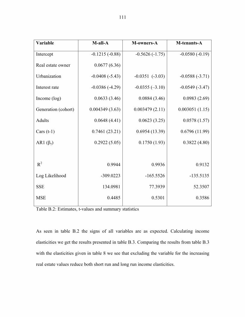
111

Variable M-all-A M-owners-A M-tenants-A

Intercept

Real estate owner

Urbanization

Interest rate

Income (log)

Generation (cohort)

Adults

Cars (t-1)

AR1 (βγ)

R2

Log Likelihood

SSE

MSE

-0.1215 (-0.88)

0.0677 (6.36)

-0.0408 (-5.43)

-0.0386 (-4.29)

0.0633 (3.46)

0.004349 (3.63)

0.0648 (4.41)

0.7461 (23.21)

0.2922 (5.05)

0.9944

-309.0223

134.0981

0.4485

-0.5626 (-1.75)

-0.0351 (-3.03)

-0.0355 (–3.10)

0.0884 (3.46)

0.003479 (2.11)

0.0623 (3.25)

0.6954 (13.39)

0.1750 (1.93)

0.9936

-165.5526

77.3939

0.5301

-0.0580 (-0.19)

-0.0588 (-3.71)

-0.0549 (-3.47)

0.0983 (2.69)

0.003051 (1.15)

0.0578 (1.57)

0.6796 (11.99)

0.3822 (4.80)

0.9132

-135.5135

52.3507

0.3586

Table B.2: Estimates, t-values and summary statistics

As seen in table B.2 the signs of all variables are as expected. Calculating income

elasticities we get the results presented in table B.3. Comparing the results from table B.3

with the elasticities given in table 8 we see that excluding the variable for the increasing

real estate values reduce both short run and long run income elasticities.

112

M-owners-A M-tenants-A

Car availability = 0.5

Car availability = 0.75

Car availability = 1.00

Car availability = 1.25

Mean car availability in the group35

Short run

0.1768

0.1179

0.0884

0.0675

0.0807

Long run

0.6963

0.3871

0.2902

0.2216

0.2649

Short run

0.1966

0.1311

0.0983

0.0786

0.1846

Long run

0.6136

0.4092

0.3068

0.2453

0.5762

Table B.3: Income elasticities for car ownership.

35 The average for real estate owners is 1.0960 cars and for tenants it is 0.5326.

113

Demand for car transport in Denmark

- Differences between rural and urban car owners

Jens Erik Nielsen

Danish Transport Research Institute

and

University of Copenhagen

Abstract

We examine how the demand for car travel in Denmark is affected by income, fuel cost,

and car purchasing cost. We use two different sources of data; The Danish Transport

Diary Survey and time series from Statistics Denmark. A partial adjustment model for

daily car transport is estimated. As in recent UK and Danish studies we find that on a

national level, car travel is more sensitive to car purchase cost than it is to fuel cost. We

offer some insight into this result by showing that car travel by urban households depends

mostly on fuel prices and car travel for rural households depend mostly on car purchase

cost. This finding is important since it helps us to understand how different transport

policies might affect households in different regions thus contributing to the

understanding of the distributional impact of the policies.

114

1. Introduction

To plan infrastructure investments and tax policies in the transport sector we need to

understand how the demand for transport evolves, what affect the demand and who is

affected by changing prices. To do so one often looks at past experiences, extrapolates

trends, and examines what cause the trend to increase or decrease. When investigating

demand for car transport there are two margins which are of interest. The first is the mode

choice, i.e. the choice on the extensive margin. The second is the choice of how much to

travel given the mode choice, i.e. the choice on the intensive margin. Investigating

behavior on both margins is important since it helps to understand the level of road

congestion which is a major concern in almost all major cities. The estimation of car

ownership in Denmark we addressed in Nielsen (2006a) and Nielsen (2006b). The

present paper is concerned with the choice of how much to travel once households have

acquired at least one car and use it. We therefore look at car trips thus focusing on the

choice on the intensive margin.

We set up a partial adjustment model for car transport and estimate it using the approach

suggested by Dargay & Vythoulkas (1999) where a partial adjustment model for car

ownership for the first time is estimated using a pseudo-panel. The approach has since

been extended in several ways to analyze car ownership decisions. Dargay (2001) allows

for asymmetric income effects in car ownership showing that hysteresis is present. She

later examines differences in car ownership between rural and urban households (Dargay

(2002)) and in Nielsen (2006a) the influence of changing real estate prices and changing

interest rates on car demand is analyzed. The method is also used in Dargay (2004) to

115

examine the price and income effects on car travel in the UK. She shows that households’

car transport is more sensitive to changes in car purchase cost than changes in user cost.

She finds short-run elasticites with regards to car purchase cost to be -0.35 and the short-

run elasticity with regards to motor fuel prices to be -0.10 with corresponding long-run

elasticities of -0.46 and -0.14. This paper extend on her findings and offer some insight

into this result by showing that for rural households car travel is sensitive to car purchase

cost and not so much to fuel cost. For urban households we find the opposite; that car

travel is sensitive to fuel cost and not so much to car purchase cost. One possible

explanation for this is that rural households have a higher need for car transport and low

possibility of changing to other means of transport. This causes their travel demand to be

affected more by the number of cars available to them (one car or more than one car)

compared to the changed use of a single car. For urban households the public transport

system is better and when fuel prices increase they can more easily change their mode of

transport and they also have shorter distances to travel than rural households.

In a Danish setting the demand for car transport has been investigated in Bjørner (1999).

He uses aggregated time series to estimate a model where he assumes that the level of

transport can be described by a Cobb-Douglas function. He finds long-run elasticities

with regard to income, fuel cost and car price to be 0.42, -0.84 and -1.12 respectively.

Surprisingly he find that income in some estimations are not significant but point out that

this might be due to multicollinearity between income, car ownership and a trend

parameter used in his specification, but as he also points out it might be that income plays

a minor role in the demand for car transport once a car is purchased. Birkeland et al.

116

(1999) use both cross-section modeling and a pseudo-panel approach to estimate income

elasticities for car transport in Denmark. The cross-section methods they use gives

income elasticities between 0.28 and 0.48 whereas the pseudo-panel method (used on a

non-dynamic model) results in an income elasticity of 0.19. A recent Danish study also

dealing with the demand for car transport is Fosgerau et al. (2004) where an aggregate

model for the Danish road transport is presented. Their model consists of several minor

models, one of which deals with the demand for car transport. They use gross national

product per capita for Denmark together with a relative price index for the running cost of

driving to estimate a partial adjustment model finding short- and long-run income

elasticities of 0.13 and 0.16 together with short- and long-run cost elasticities of -0.30 and

-0.37. They also address the problem of saturation in car ownership in Denmark

concluding that saturation effects are not likely to affect the development in car

ownership in Denmark, since the car ownership per capita is still well below that of other

countries. This is confirmed by figures from EuroStat where Denmark is one of the

countries with the lowest amount of cars per 1.000 inhabitants (350 cars per 1.000

inhabitants. See Dargay et al. (2006) for details)

A recent paper dealing with the development in car transport is Kwon and Preston (2005).

They use data from the National Travel Survey in the UK to decompose the effect of

increased travel distance into what they call ‘car ownership effects’ (changes caused by

changing car ownership) and ‘car use effects’ (changes in car use dependent on car

ownership level)36. They find that ‘car ownership effects’ explain about half of the

36 In our work we label these effects ‘intensive effects’ and ‘extensive effects’ in order to use the same methodology as is used in other economic papers, especially literature dealing with the labor-market where

117

growth in car trip distance but also that this trend seems to be going down possibly

because of saturation effects. They also identify two trends affecting the ‘car use effects’

namely increasing number of trips and increasing trip lengths. The first of these were

dominating in the 1970s and 80s whereas the latter seems to dominate in the 90s.

Furthermore they identify several factors affecting these effects and they present a survey

of some recent fuel price elasticities for car transport reporting a consensus of -0.15 in the

short run and -0.30 in the long run. These findings are higher than those reported by

Dargay (2004) and also higher than what we find for long run fuel cost elasticities in the

present paper.

Our paper adds to the literature in two ways. It offers new insights into the influence of

car purchase prices and fuel prices on car travel found in both Denmark and in the UK.

Secondly, since the data used by Dargay in the UK studies did not include information on

the distance traveled but calculated a proxy for this variable from household expenditure

data, average fuel price data, and data on the average fuel efficiency of cars, one could

question the reliability of the UK results. By using a different type of data, namely a

transport survey where the needed variables are available, we obtain results comparable

to those found for the UK thus verifying the approach used in these studies. This is

important since large transport surveys are rarely available and household expenditure

surveys are.

‘intensive responses’ capture effects on the number of working hours and ‘extensive responses’ describe the labor market participation decisions (see for example Kleven and Kreiner (2006)).

118

This paper has the following structure. The next section presents the data and describes

the construction of the pseudo-panel. Section 3 describes the model, section 4 presents

the estimation and section 5 derives price and income elasticities. The final section

concludes.

2. The data and the pseudo-panel

We use data from the Danish Transport Diary Survey together with time series from

Statistics Denmark for the period from 1995 to 2002. The survey is conducted on a

monthly basis with 1800 people between 16 and 74 being sampled from the Danish

Central Personal Register every month until 1997. From 1998 the sample is extended to

include people from age 10 to 84 and the sample size is increased to 2100 persons per

month. The response rate is between 65% and 70%. Information on a given day of travel,

including transport mode, distance traveled, trip chaining, and time use. Background

information about the interviewee and her household is also collected (income, number of

adults and children, car ownership, employment, etc.) together with a series of

geographical variables37. We do not use all the observations in the survey. Since our

focus is on the distance traveled by car we exclude all households not owning at least one

car. Observations with missing variables are also excluded from the sample. From

Statistics Denmark we obtain time series for car purchase costs and fuel costs for the

years 1995 to 2002.

37 A full description of the data can be found at the homepage of the Danish Transport Research Institute, www.dtf.dk.

119

Using the procedure described by Deaton (1985) we construct a pseudo-panel for cohorts

for the years 1995 to 2002. We use three characteristics to create our panel; year of birth

of the interviewee, real estate ownership status, and urbanization. The year of birth is

often used when pseudo-panels are created and we choose the remaining characteristics

since we want to examine differences between urban and rural households and since it

was shown in Nielsen (2006a) that real estate ownership could influence the demand for

cars. Creating the pseudo-panel according to these variables thus reduce the variation

within the cohort-group and thus reduce the loss of information caused by the aggregation

to cohort levels (See Deaton (1985) for a discussion of this). We thus end up with cohort-

observations for four types of households; urban real estate owners, rural real estate

owners, urban tenants, and rural tenants. With 11 cohorts we therefore have a total of 44

observations for each of the years between 1995 and 2002.

In figure 1 we see that the distances traveled by car depend on both the degree of

urbanization and the cohort. The fact that the urbanization level influences the travel

distance by car is not surprising since distances in general are longer in rural areas than in

urban areas and since public transport services are better in urban areas. Urban

households thus have better substitutes for car travel than rural households. Differences in

the traveled distance only seem to be present for the younger cohorts though. For persons

over the age of 55 the traveled distance still depends on the cohort but the effect of the

level of urbanization seems to disappear.

120

Figure 1: Distance traveled by car in urban and rural areas by different cohorts,

contingent on the households having at least one car.

Source: Danish Transport Diary Survey.

Incomes are also different for urban and rural households with urban households having

higher income than rural households as shown in figure 2. We also see that the income

differs between cohorts with income rising until a person turns 50 and a large drop in

income when the person passes 60 and retires. These differences are to a large extent due

to life-cycle effects but some cohort-effects are also present with young generations

having higher salaries than the older generations had when they were young.

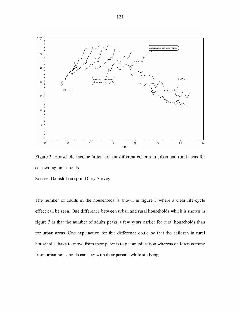
121

Figure 2: Household income (after tax) for different cohorts in urban and rural areas for

car owning households.

Source: Danish Transport Diary Survey.

The number of adults in the households is shown in figure 3 where a clear life-cycle

effect can be seen. One difference between urban and rural households which is shown in

figure 3 is that the number of adults peaks a few years earlier for rural households than

for urban areas. One explanation for this difference could be that the children in rural

households have to move from their parents to get an education whereas children coming

from urban households can stay with their parents while studying.

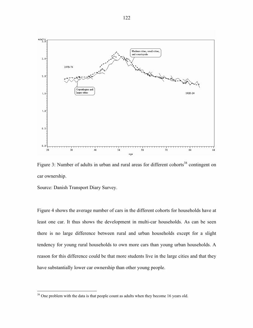
122

Figure 3: Number of adults in urban and rural areas for different cohorts38 contingent on

car ownership.

Source: Danish Transport Diary Survey.

Figure 4 shows the average number of cars in the different cohorts for households have at

least one car. It thus shows the development in multi-car households. As can be seen

there is no large difference between rural and urban households except for a slight

tendency for young rural households to own more cars than young urban households. A

reason for this difference could be that more students live in the large cities and that they

have substantially lower car ownership than other young people.

38 One problem with the data is that people count as adults when they become 16 years old.

123

Figure 4: Car ownership for urban and rural households, contingent on households having

at least one car.

Source: Danish Transport Diary Survey.

Figure 5 shows the development in both fuel price and purchase price for cars between

1993 and 2002. We see that car prices have increased slightly in the period whereas fuel

prices have fluctuated more with a huge increase from 1998 to 2000.

124

0

20

40

60

80

100

120

140

1993 1993 1994 1995 1996 1997 1998 1998 1999 2000 2001 2002Year

Pric

e in

dex

(200

0=10

0)

Fuel priceCar price

Figure 5: Price index for fuel price and car purchase cost (2000=100).

Source: Statistics Denmark.

3. The model

We use a model based on Dargay and Vythoulkas (1999) with a semi-log specification

for income. Our choice of semi-log specification is based on the findings of Dargay

(2001) where different specifications were tested (Linear, Double-log and Semi-log)

concluding that the semi-log specification was the preferred one. Letting itC represent the

number of kilometers driven at time t for household i, itY the annual after tax income for

household i at time t, tT is the average purchase price for cars at time t, itU is a dummy

for households living in urban areas, tF is the average fuel price at time t, itI the number

125

of adults in the household, and with iG being the cohort number, the demand for car

travel is determined by

1log( )i i i i i i it Y t T t U t F t I t G C t tC Y T U F I G Cα β β β β β β β ε−= + + + + + + + + (1)

where α is a constant and itε is an term following a normal distribution,

2(0, ( ) )i it tNε σ∼ .

Since we use a pseudo-panel approach as described in Deaton (1995) all our variables

take the form itct

A ctn

iA=∑ where c

tn is the number of households in cohort c and ctA is the

variable. We let itC represent daily car transport in kilometers in year t for cohort i,

itI

the number of adults in the household, i

G the cohort number, tF the fuel price, itY the

annual after tax income, itU is a dummy for households living in urban areas, and tT is

the average purchase price for cars.

In order to determine if autocorrelation is present we use the Durbin-h statistics and the

Durbin-t statistics. The results for the three models are shown in table 1.

M-all M-urban M-rural

Durbin-h

Durbin-t

-0.2776 (0.3907) -2.8589 (0.0021)

1.1436 (0.1274)

Table 1: Test statistics for the presence of autocorrelation.

126

As we can see in the M-all model and the M-rural model we get a strong indication that

we can proceed under the assumption of autocorrelation. For the M-urban model the

result is less clear but we have estimated the model with several lags and all parameters

are insignificant. We thus conclude that we can proceed under the assumption of

autocorrelation.

The statistical model can thus be written as

1

2

log( )

(0, ( ) )

i ii i i it t tt tt Y T U F I t G C t

it t

C Y T U F I G C

N

α β β β β β β β ε

ε σ

−= + + + + + + + +

∼

(2)

where 1itC − is the number of cars in the previous period and tε is an error term39.

Estimating the model shown in (2) directly on the pseudo-panel described in section 2

would result in the problem of hetehoscedasticity since the variance of the error-run will

be given by

21 1 1 1( ) ( ) ( ) ( ) ( ) ( )c c c ct t t t

i i i i it t t t tn n n n

i iVar Var Var Var Varε ε ε ε ε= = = =∑ ∑ (3)

and thus be dependent on the number of observations in each of the cohorts. In order to

avoid this we simply multiply all cohort-observations with the square root of the number

of observations used in the given cohort thus getting

21 1 1( ) ( ) ( ) ( ) ( ) ( )c c ct t t

ic c i c i c i itt t t t t t t tn n n

i iVar n Var n Var n Var n Varε ε ε ε ε= = = =∑ ∑ (4)

39 A test for the presence of autocorrelation showed that in most cases we could proceed with the simple error structure shown in (2).

127

and thus having a model where heteroscedasticity is eliminated. We therefore assume that

all the error terms follow a normal distribution with the same variance σ2 as in (1). As

argued by Dargay and Vythoulkas this model can be estimated using standard techniques.

4. Estimation

The variables used can be seen in table 2 together with their sources.

Variable Source Description

Urbanization

Income (log)

Cohort

Adults

Car purchase price

Fuel price

Transport demand

DTDS

DTDS

DTDS

DTDS

SD

SD

DTDS

Dummy for living in a large city

Logarithm of household income

Cohort number

Number of adults in the household

Price index for car purchase cost

Price index for fuel cost

Daily transport demand in kilometers

Table 2: Variables used in the model (Source: Statistics Denmark (SD), Danish Transport

Diary Survey (DTDS))

In table 3 the number of observations used to construct the pseudo-panel is shown. We

have defined urban households as households living in one of the five largest cities in

Denmark and rural areas are thus the remaining households. Since the number of

observations in each cohort should be as large as possible we are faced with a tradeoff

since increasing the number of observations reduces the number of cohorts we can

128

construct. Here we have chosen 5-year bands for each cohort but still the average number

of observations for tenants are low.

Cohort

number

Cohort date

of birth

Urban

owner

Rural

owner

Urban

tentants

Rural

tenants

1

2

3

4

5

6

7

8

9

10

11

1920-24

1925-29

1930-34

1935-39

1940-44

1945-49

1950-54

1955-59

1960-64

1965-69

1970-74

291

502

695

880

1237

1500

1277

1314

1259

1081

614

936

1707

2293

3026

4080

5010

4676

4430

4337

3709

1989

198

303

319

372

375

431

335

427

578

803

762

170

288

298

278

314

390

375

421

509

744

812

Cohort average 968 3290 446 418

Table 3: Number of observations

Using the pseudo-panel to estimate the model, remembering that we multiply each

cohort-observation with the number of observations used to construct it, we get the

results shown in table 4.

129

Variable M-all M-rural M-urban

Constant

Urbanization

Income (log)

Adults

Car purchase price

Fuel price

Cohort

Transport demand

R2

Log Likelihood

SSE

MSE

-0.0056 (-0.00)

-6.3271 (-6.39)

9.4187 (3.67)

2.9518 (1.69)

-0.3357 (-3.07)

-0.0425 (-2.40)

1.5164 (7.82)

0.2025 (3.52)

0.9535

-1661.3546

1213776.56

4185

12.4345 (0.75)

10.5508 (2.75)

3.2965 (1.44)

-0.4316 (-2.62)

-0.0256 (-1.08)

1.4793 (5.27)

0.2332 (2.71)

0.9580

-850.2932

789693.948

5561

-70.3248 (-3.10)

4.2964 (1.19)

1.2177 (0.41)

0.0533 (0.32)

-0.0703 (-2.50)

1.6192 (6.33)

0.0270 (0.35)

0.8896

-792.6594

364321.752

2566

Table 4: Estimates, t-values and summary statistics

Most of the variables are significant but we see that income and the number of adults in

the urban households is insignificant. For income this correspond to the findings in

Bjørner (1999) where income was found to be insignificant in some instances. Signs of

the variables are also as expected with the exception of car purchase prices in the model

for urban households but this variable is not statistically significant. For rural households

the variable for fuel price is not significant. One possible explanation is that rural

households, having poor access to public transport and longer distances to travel are more

130

dependent on their car for all trips and especially trips which are necessary (like

commuting trips, essential shopping trips, and leisure trips where the distances makes

other modes of transport than car impractical). Such trips could potentially be a large part

of the trips undertaken for rural households. This is not the case for urban households

where the distances are shorter and the public transport network is a good substitute for

car transport. Even though we do not see great differences between rural and urban

households when it comes to the number of cars available in car-owning households (see

figure 3) the effect of changing prices on the purchase of cars only seems to affect the car

transport of rural households and not that of urban households. The estimation also shows

that cohort effects are present and younger generations travel longer than older

generations. Except for the urban households the adjustment parameter is also significant

but with values of 0.20 and 0.23 we see that around 80% of the adjustment in transport

demand happens within the first year. For rural households the adjustment parameter is

0.03 and adjustment is almost instantaneous which also explains why the parameter is not

statistically significant.

5. Elasticities

To calculate the elasticities for Denmark we use the M-all model. The formula for short

run elasticities of car transport with regards to variable xi is given by i i

ii

x xsr Ci xx C Cε β∂

∂= =

and the corresponding long run elasticity can be calculated as SRi

i

LRi

εθε = where θi=(1-βi)

is the adjustment parameter. Estimated short- and long-run elasticities are shown in table

5.

131

Income Car purchase price Fuel price

Short run

0.25

Long run

0.32

Short run

-0.90

Long run

-1.13

Short run

-0.11

Long run

-0.14

Table 5: Elasticities for the complete model40

With the adjustment parameter being relatively high (θi=7975) the difference between

short- and long-run elasticities are not large. The income elasticities found here is in line

with some findings in Birkeland et al. (1999) but lower than those found in Bjørner

(1999) and Fosgerau et al (2004). Our income elasticities are much lower than those

reported for UK in Dargay (2004) where values around 1 are found. For the elasticity

with regard to car purchase cost our results are comparable with those found in Bjørner

(1999) but our fuel price elasticity is substantially below his finding but in line with the

findings in Birkeland et al. (1999) and Dargay (2004).

Rural households Urban households

Income elasticity

Car purchase price elasticity41

Fuel price elasticity42

Short run

0.27

-1.09

Long run

0.35

-1.42

Short run

0.14

-0.23

Long run43

0.14

-0.23

Table 6: Elasticities for rural and urban households44

40 We assume that the number of kilometers traveled is 36 which is the average in 2000. The price index for the purchase price for cars was 100 in 2002 and the price index for fuel was 100. 41 The car purchase price is only significant for rural households. 42 The fuel price is only significant for urban households 43 For urban households the income parameter and the adjustment parameter are insignificant. With an adjustment parameter close to 1 we thus have almost identical short- and long-run elasticities.

132

Using the models for urban and rural households we get the results shown in table 6. As

in Christens and Fosgerau (2004) that urban households have higher income elasticity

than rural households but we also keep in mind that their elasticities were for car

ownership and our elasticities are for travel by car. For the two groups the elasticities

with regard to car purchase price and fuel price increase numerically compared to the

elasticities shown in table 5.

6. Conclusion

Other studies have estimated the demand for car transport for Denmark but in this paper

we for the first time utilize the Danish Transport Diary Survey to create a pseudo-panel

and use this to estimate a dynamic partial adjustment model for car transport. Other

dynamic specifications have used aggregate time series or based their estimates on cross-

section methods. Elasticities for car transport are found with regard to income, car

purchase cost and fuel price.

We show that urban households respond more to changing fuel prices than to changes in

the purchase price of cars. The opposite holds for rural households where the demand for

car transport is more sensitive to changes in the purchase price of cars than to changing

fuel prices. Our result supports the findings of Dargay (2004) where the UK Family

Expenditure Survey is used to estimate a dynamic model for car transport. She

constructed a proxy for car transport and it is thus interesting to see, if a different type of

data gives comparable results. Finding that the different data yield similar results is

44 We assume that the number of kilometers traveled is 39.7 for rural households and 30.9 for urban households which is the average in 2000. The price index for the purchase price for cars was 100 and the price index for fuel was 100 in 2000.

133

important since many countries have large expenditure surveys but do not have large

transport surveys. Using expenditure surveys in future work thus seems to be justified.

134

References

Birkeland, M. E., Brems, C. R. and Kabelmann, T. (2000) Analyse af personers

transportarbejde, 1975-1998, Trafikdage på Aalborg Universitet 2000, Conference paper

(www.trafikdage.dk)

Bjørner, T. B. (1999) Transport Demand and Environmental Regulation in the Transport

Sector, Ph.D. dissertation, University of Copenhagen, Department of Economics, Red

Series number 54.

Christens, P. F. and Fosgerau, M. (2004) Rådighed over bil - en beskrivelse af

sammenhængen mellem husstandsindkomst, bilrådighed og geografi, DTF Notat 3 2004,

Danish Transport Research Institute, www.dtf.dk.

Dargay, J. M. and Gately, D. (1999) Income’s effect on car and vehicle ownership,

worldwide: 1960-2015, Transportation Research Part A 33, 101-138.

Dargay, J. M and Vythoulkas, P. C. (1999) Estimation of a Dynamic Car Ownership

Model: A Pseudo-panel Approach, Journal of Transport Economics and Policy 33:3,

287-302.

Dargay, J. (2001) The effect of income on car ownership: evidence of asymmetry,

Transportation Research Part A 35, 807-821.

Dargay, J. (2002) Car ownership in rural and urban areas: a pseudo-panel analysis,

Transportation Research Part B 38, 351-366.

Dargay, J. (2004) The Effect of Prices and Income on Car Travel in the UK, World

Conference on Transport Research, Istanbul, Turkey, July 2004.

135

Dargay, J., Hivert, L. and Legros, D. (2006) The dynamics of car ownership in E.U

countries: a comparison based on the european household panel survey, unpublished

working paper.

Deaton, A. (1985) Panel Data from Time Series of Cross Sections, Journal of

Econometrics 30, 109-126.

Fosgerau, M., Holmblad, M. and Pilegaard, N. (2004) ART – En aggregeret

prognosemodel for dansk vejtrafik, Notat 5 2004, Danish Transport Research Institute.

Kleven, H. J. and Kreiner, C. T (2006) The Marginal Cost of Public Funds: Hours of

Work Versus Labor Force Participation, The Journal of Public Economics,

Forthcomming.

Kwon, T-H, and Preston, J. (2005) Driving Forces behind the Growth of Per-capita Car

Driving Distance in the UK, 1970-2000, Transport Reviews 25:4, 467-490.

Nielsen, J. E. (2006a) Real estate ownership and the demand for cars in Denmark – A

pseudo-panel analysis, Thesis Paper.

Nielsen, J. E. (2006b) Estimating car ownership in Denmark – Discrete choice modeling

and repeated cross-section analysis, Thesis Paper.

Nielsen, J. E. (2006c) Transport tax reform, two-part tariffs and revenue recycling, Thesis

Paper.

136

137

Transport tax reforms, two-part tariffs, and revenue

recycling

Jens Erik Nielsen

Danish Transport Research Institute

and

University of Copenhagen

Abstract

We explore the interaction between taxes on the purchase of cars and on the use of cars

when households face a discrete choice of purchasing a car or not. We use a simple labor-

leisure model with a logit formulation for the discrete choice of car-ownership to examine

how a tax reform which shifts taxes from car ownership to use of cars affects welfare. To

our knowledge this is the first time the discrete nature of car purchase is modeled

explicitly in a tax-reform model and it is thus the first consistent analysis of a tax reform

involving both fixed and variable cost. Car transport is associated with negative

externalities and feedback effects. We show that the welfare effect of this type of reform

depends on both the choices of car usage and car ownership decisions and that feedback

effects exist on both the intensive margin and on the extensive margin. Furthermore the

effect of such a tax reform depends on the initial level of the variable tax on car transport

relative to the pigouvian level. The findings are illustrated by simulations.

138

1. Introduction

The importance of intervention in the transport sector has become obvious in recent years

with externalities, and especially congestion externalities, increasing rapidly in almost

every major city. The dilemma facing the transport authorities is that transport, while

causing negative externalities, is an essential part of social life and that increasing

transport seems to be closely related to economic growth. One aspect of this dilemma is

pointed out in Parry & Bento (2001). They show that the implementation of marginal cost

pricing to reduce externalities can cause negative welfare effects if the extra costs of

transport discourage labor supply. A similar insight is obtained in Nielsen (2006a) where

the optimal tax rules in a Becker (1965) framework for household time allocation are

derived for a situation with atmospheric externalities. Here it is shown that the additivity

property derived by Sandmo (1975) still apply, though in a modified form thus extending

the findings of Kleven (2004) where an inverse factor share rule was derived in a Becker

framework. An important insight from the Parry and Bento paper is that we have to be

careful when we evaluate the welfare effects of tax reforms in the transport sector, since a

tax which seems to be optimal when analyzed in isolation (in their case marginal cost

pricing) could have negative welfare effects if analyzed in a general equilibrium setting.

In this paper we examine a tax reform in the transport sector involving a fixed cost of

purchasing (or owning) cars. A fixed purchase (or ownership) tax on cars is replaced by a

variable tax on the use of cars in a budget neutral way. In order to analyze this reform one

needs to account for car ownership decisions (e.g. decisions on the extensive margin).

Reforms of this kind are frequently suggested in the Danish debate since the marginal tax

139

on the purchase of cars in Denmark is 180% (DORS (2006)). This type of tax reforms

have to our knowledge not yet been analyzed consistently, since the discrete nature of the

car ownership decision has been left out of previous analysis.

We build upon several results from the economic literature. The explicit inclusion of time

in economic models was first undertaken by Becker (1965), DeSerpa (1971), and

others45. They include time as a source of utility for households, either directly in the

utility functions (DeSerpa), or indirectly through a household production function

(Becker). For the modeling of car ownership, we draw upon the results from Small and

Rosen (1981). Based on the work of McFadden (1974) they present a framework for

modeling welfare effects when discrete consumer choices have to be taken into account.

De Borger (2000) demonstrates that the Small & Rosen approach can be implemented in

a tax model, and he uses their framework to derive the optimal two-part tariff in a model

of discrete choice which he extends to a situation with externalities in De Borger (2001).

Unfortunately the time allocation problem and thus the labor-leisure tradeoff is not

included in these papers.

The modelling framework used here is based on Parry and Bento (2001). They construct

a general equilibrium model for commuting transport, labor supply, and congestion

externalities in order to analyze tax reforms involving variable taxes on the use of cars,

subsidies to public transport (in their model a metro system), and reduction in labor taxes.

They show that interactions with pre-existing taxes are important and that feedback

effects influence the welfare effects of the tax reforms. They use the same framework in 45 A recent survey on the literature on time allocation can be found in Jara-Díaz (2003)

140

Parry and Bento (2002) to analyze situations with different types of externalities and

interactions with different types of taxes. Again they conclude that welfare effects of tax

reforms depend on interactions with pre-existing distortions in the economy. De Borger

and Van Dender (2003) use the same framework to analyze the effect of a tax reform on

the value of time. They show that commuting taxes might reduce the value of time while

taxes on non-commuting traffic plausibly raise the value of time. They thus demonstrate

that the tax system and time values are closely related; a finding which was also pointed

out earlier in Forsyth (1980).

In this paper we show that the welfare effect of a tax reform depends on a combination of

several factors, some of which are identified in the papers mentioned above. The new

finding is that changes on the extensive margin (e.g., changes in car-ownership) could be

large and should be modeled explicitly if correct estimates of welfare effects are to be

obtained. With the use of simulation, we demonstrate that it is possible to include discrete

effects and we believe that future evaluation of tax reforms in the transport sector should

include these or at least reflect on the consequences of not including extensive responses.

Furthermore our simulation shows that the optimal tax on the use of cars is equal to the

marginal external damage cost, i.e. the pigouvian tax rate.

The paper has the following structure. Section 2 presents the modeling framework in

which household decisions on the intensive margin (how much to consume contingent on

car-ownership) is analyzed and the choice on the extensive margin (the car-ownership

decision) is also described in detail. The production sector and the government

141

optimization problem are also presented. Section 3 derives an expression for the welfare

effect of a tax reform involving a shift from fixed to variable taxation of cars. Section 4

simulate a tax reform to illustrate the theoretical findings. The final section concludes.

2. The model

Inspired by Parry and Bento (2001) we construct a model where households decide on the

consumption of goods and leisure and they also choose how much to work and if they

want to commute by private transport ('car') or public transport ('metro'). Our model

deviates from previous models of this type since we do not assume households to be

identical. Instead we assume that all the observable socioeconomic characteristics of the

households are identical and it thus seems as if they have identical utility functions.

Observing the outcome of the households' actions their choice of car-ownership is not

consistent with the households being identical since some households purchase a car and

others do not. Their choice thus appears to be random. The households can therefore be

divided into two types: those who do not purchase a car and those who purchase a car.

We assume that households purchasing a car can commute by either car or metro.

Households not purchasing a car can only commute by metro. Furthermore we assume

that congestion externalities are present in 'car transport'.

The production sector in this economy is fully competitive and operates under constant

returns to scale. All producer prices are therefore constant and equal to the marginal cost

of production. The government taxes goods, transport and labor income in order to

generate revenue for some unspecified tasks (e.g. national defense or the health care

system).

142

2.1 The households

Households consume 'pure leisure', L, an aggregate consumption commodity, Z, public

transport (a metro service), and private transport (car transport). Households also supply

labor to the production sector and can go to work by either metro or car. We assume that

consumption of the aggregate good and consumption of leisure as well as 'transport' in

itself generates household utility and we write the individual households utility function

as

( , ) ( , )b cU L Z u Z Z+ (1)

where bZ is trips by metro and cZ is trips by car. These are defined in detail below. The

separability assumption between U and u in (1) separates the choice of transport mode

from the decision on how much to work. It also allows for imperfect substitutability

between transport by metro and transport by car. This seems like a realistic assumption

since some people dislike crowded metros and enjoy the privacy of their own car.

We assume that H households exist and that H is large. All households have the same

earning capacity and thus the same wage rate w. Furthermore all households have the

same endowment of time, L , and non-labor income, y. Each commuting trip takes up a

certain amount of household time which we will denote bL for a trip by metro and cL for

a trip by car. A trip is defined as traveling both to and from work. This means that

households either go back and forth by car or by metro. Following Parry & Bento (2001)

we assume that the number of working hours in one day is fixed and equal to one. This

means that the supply of labor hours given by wL is equal to the total number of

commuting trips

143

w b cL Z Z= + (2)

We let Z be total number of trips by car and assume that, because of congestion, a higher

value of Z increases the time requirement for car transport. We thus have that

( )' 0cL ZZL ∂

∂= > (3)

Assuming that households ignore their own influence on Z , we have an externality

problem in car transport. We assume that the metro service is not affected by congestion.

Letting P , bP , and cP represent consumer prices on goods, metro trips and car trips, wt

the tax on labor, and P be the fixed cost of purchasing a car. Normalizing the wage rate

w to one then allows us to write the constraints which the households face as

{ 0} (1 )cb b c c w

wZPZ P Z P Z P t L y>+ + + Ι = − + (4)

b b c c wL L Z L Z L L+ + + = (5)

where { 0}cZ >Ι is an indicator function equal to 1 if 0cZ > and zero otherwise. It therefore

indicate whether the households purchase a car or not. Following DeSerpa (1971) we will

label (4) the budget constraint and label (5) the time resource constraint. The constraints

are interdependent through wL , bZ , and cZ . Apart from the fixed cost, P , and the fact

that households can make a choice on the extensive margin with regards to car

ownership, this part of the model is similar to the one used in Parry & Bento (2001).

2.1.1 The choice at the intensive margin

We now examine how a household behaves conditional on its choice of car ownership

status. Since households owning a car and households not owning a car can choose

144

between different consumption bundles ('non-owners' can not choose to travel by car) and

face different budget constraints ('owners' have to pay a fixed fee P ), we analyze the two

types of households separately.

2.1.1.1 The choice for car owners

Letting subscript 1 indicate car ownership, using the constraint given in (4) and (5), and

remembering that the households ignore their own influence on the level of Z we can

specify the utility maximization problem for car owners as

1 1 1 1

1 1 1 1

, , ,

1 1 1 1 1

1 1 1 1 1

max ( , ) ( , )

. .

(1 ) ( )

( ) ( )

b c

b c

L Z Z Z

b b c c w Mw

b b c c w T

U L Z u Z Z

s t

PZ P Z P Z P t L y

L L Z L Z Z L L

λ

λ

+

+ + + = − +

+ + + =

(6)

where 1Mλ is the marginal utility of income, 1Tλ is the marginal utility of time as a

resource, and labor supply will be given by

1 1 1w b cL Z Z= + (7)

With (6) being a standard maximization problem the first order conditions are given by

11

TUL

λ∂∂

= (8)

11

MUZ

Pλ∂∂

= (9)

1 11 ( (1 )) ( 1)M b T b

wbu

ZP t Lλ λ∂

∂= − − + + (10)

1 11 ( (1 )) ( ( ) 1)M c T c

wcu

ZP t L Zλ λ∂

∂= − − + + (11)

together with the budget constraint (4) and the time resource constraint (5).

145

Following De Serpa (1971) we define the value of time for car owners, 1VoT , as 1

1

UL

UZ

∂∂

∂∂

and by using (8), (9), and (11) we can write this as

1 1 11

((1 ) )

( ) 1

1 cwT M

cM

t P

L Z

ucZ

VoT λλ

λ+ − −

+

∂∂

= =

(12)

or by using (10) instead of (11) we can write it as

1 1 11

((1 ) )

1

1 bwT M

M b

t P

L

ubZ

VoT λλ

λ+ − −

+

∂∂

= =

(13)

The numerator of (12) and (13) measure the value of one days work. To see this note that

1cu

Z∂∂

and 1bu

Z∂∂

measure the marginal utility of a trip by car or metro respectively. By

dividing with 1Mλ this is converted into monetary terms. One days work also generates

income and there is a price on commuting. This is captured by ((1 ) )cwt P− − and

((1 ) )bwt P− − which is the income from one days work consisting of the after tax income,

(1 )wt− , and the price of the commuting trip, bP or cP . The denominator measure the

time used on a days work which consist of the time spend working (which we normalized

to one) and commuting time. We thus see that (12) and (13) describes the value of time

for car owners. From (12) and (13) we get that a tax on commuting working through

either bP or cP reduce the value of time, which is also pointed out in De Borger and Van

Dender (2003). It is also obvious that a reduction of the labor tax, wt , will increase the

value of time and increased congestion reduce the value of time. The expressions in (12)

and (13) for the value of time resemble those found in De Borger and Van Dender (2003),

and as they note the value of time is independent of the activity in which it is used.

146

Using the first order conditions (8) through (11) together with the budget constraint (4)

and the time resource constraint (5) we get the ordinary demand functions for car owners

1( , , , , , ( ), , , )b c b cwL P P P t L L Z y P L (14)

1( , , , , , ( ), , , )b c b cwZ P P P t L L Z y P L (15)

1( , , , , , ( ), , , )b b c b cwZ P P P t L L Z y P L (16)

1( , , , , , ( ), , , )c b c b cwL P P P t L L Z y P L (17)

together with shadow prices 1Mλ and 1Tλ . Using these together with

1 1 1w b cL Z Z= + (18)

we can write the indirect utility function for households owning a car as

1 1 1 1

1

1 1 1 1

, , ,

1 1 1 1 1

1 1 1 1 1

( , , , , , ( ), , , )

max { ( , ) ( , )

( (1 ) )

( ( ) )}

b c

b c b cw

b c

L Z Z Z

M b b c c ww

T b b c c w

V P P P t L L Z y P L

U L Z u Z Z

PZ P Z P Z P t L y

L L Z L Z Z L L

λ

λ

= +

− + + + − − −

− + + + −

(19)

which is now given as a function of variables exogenous to the household.

2.1.1.2 The choice for non-car owners

Letting subscript 0 indicate non-ownership of cars, households not owning a car have to

solve

0 0 0

0 0 0

, ,

0 0 0 0

0 0 0 0

max ( , ) ( ,0)

. .(1 ) ( )

( )

b

b

L Z Z

b b w Mw

b b w T

U L Z u Z

s tPZ P Z t L y

L L Z L L

λ

λ

+

+ = − +

+ + =

(20)

where 0Mλ is the marginal utility of income, 0Tλ is the marginal utility of time as a

resource, and labor supply will be given by

147

0 0w bT Z= (21)

With (20) being a standard maximization problem the first order conditions are given by

00

TUL

λ∂∂

= (22)

00

MUZ

Pλ∂∂

= (23)

0 00 ( (1 )) ( 1)M b T b

wbu

ZP t Lλ λ∂

∂= − − + + (24)

together with the budget constraint (4) and the time resource constraint (5).

As before we follow DeSerpa (1971) define the value of time for non-car owners, 0VoT ,

as 0

0

UL

UZ

∂∂

∂∂

. By using (22), (23), and (24) we can write this as

00

0 00

((1 ) )

1

bwT M

M b

t P

L

ubZ

VoT λλ

λ+ − −

+

∂∂

= =

(25)

As in (12) and (13) the numerator is the value of one days work and the denominator is

the time used on one days work. Again we see that a tax on commuting (in this case

public transport) raise the cost of travel through bP and this reduce the value of time. It is

also obvious that a reduction of the labor tax, wt , will increase the value of time. From

(13) and (25) we also see that if the government implement a policy where the time

requirement for public transport, bL , is reduced the value of time for both car owners and

non-car owners will go up46.

46 In Copenhagen such a policy could be the opening of the new metro line in 2007 and the extension of the metro system with a city ring expected to be build during the next 10 years.

148

The problem in (20) is structurally identical to (6). As before we get the ordinary demand

functions for non-car owners

0 ( , , , , , )b bwL P P t L y L (26)

0 ( , , , , , )b bwZ P P t L y L (27)

0 ( , , , , , )b b bwZ P P t L y L (28)

together with shadow prices 0Mλ and 0Tλ . Again we can write the indirect utility

function for households not owning a car as

0 0 0

0

0 0 0

, ,

0 0 0 0

0 0 0 0

( , , , , , )

max { ( , ) ( ,0)

( (1 ) )

( )}

b

b bw

b

L Z Z

M b b ww

T b b w

V P P t L y L

U L Z u Z

PZ P Z t L y

L L Z L L

λ

λ

= +

− + − − −

− + + −

(29)

which is now given as a function of variables exogenous to the household.

2.1.2 The choice at the extensive margin

Facing the price structure ( , , , )b cP P P P , wage tax wt , having non-labor income y, facing

time requirements bL and cL together with externality level Z , the household chooses

between the utility level 0V and 1V given in (19) and (29). Since households are utility

maximizing, they each choose {0,1}i∈ such that

0 1max{ , }iV V V= (30)

Using the random utility approach pioneered by Daniel McFadden (McFadden (1974))

we assume that the households behave as if the indirect utility function is composed of an

observable deterministic part, iV , together with stochastic error term, iε . We write this

as i iV ε+ . The error term captures the unobservable characteristics which make the

149

household choice seem random to the government. For simplicity and to ensure a closed

form solution, we assume that these error terms are independently and identically

distributed following a double exponential distribution with scale parameter η which we

will normalize to 1. This gives us a logit model for discrete choice47,48 . We know (Ben-

Akiva & Lerman (1985) and Train (2003)) that the probability of choosing not to buy a

car, 0π , and the probability of choosing to buy a car, 1π , are given by49

0 0

0 1( , , , , , ( ), , , )b c b cw

V

V Ve

e eP P P t L L Z y P Lπ

+= (31)

1 1

0 1( , , , , , ( ), , , )b c b cw

V

V Ve

e eP P P t L L Z y P Lπ

+= (32)

It is worth noting that the probabilities shown in (31) and (32) depend on all the

parameters in the model. This means that even though households not owning a car do

not directly affect the total level of congestion, by changing behavior on the intensive

margin they still indirectly affect the level of congestion, via their impact on the extensive

margin. The expected maximum utility W for a representative household is given by50

0 1

ln( )V VW e e= + (33)

47 Further details about the logit model, the double exponential distribution and a discussion of the scale parameter η can be found in Ben-Akiva and Lerman (1985) and Train (2003). 48 A discussion of the restrictiveness relating to the choice of the double exponential distribution of the error terms can be found in appendix C of De Borger (2000). 49 From Train (2003) we have that

0 0 1 0( ) 00 0 0 1 1 1 0 0 1 0 0

0 1Pr( ) Pr( ) ( )V V V

V Ve e e

e eV V V V e e e d

ε εεπ ε ε ε ε ε− + − −− − −

+= + > + = < + − = =∫

and thus that 1 0 1

0 11 V

V Ve

e eπ π

+= − = .

50 From Train (2003) we get that the maximum expected utility for a representative household is given by 0 10 0 1 1[max{ , }] ln( )V VE V V e eε ε+ + = +

150

which is also known as the log-sum. The demand for goods and commodities for a

representative (or average) household as well as the supply of labor can now be written as

0 0 1 1Z Z Zπ π= + (34)

0 0 1 1b b bZ Z Zπ π= + (35)

1 1c cZ Zπ= (36)

0 0 1 1w w wL L Zπ π= + (37)

which is a weighted average of the demand for the two types of households in the

economy. By defining ( )bL Z as a function of c

Z instead of Z we have that (36) plays

the role of the total number of trips by car in the economy, i.e. c

Z Z= . As expected we

see that the level of Z depend on both the choice on the intensive margin, 1π , and the

choice on the extensive margin, 1cZ which is an extension compared to previous models

where the level only depend on the choice on the extensive margin. To simplify notation

we will make the assumption that c

Z Z= in the coming derivations.

2.2 The production sectors and the government

We assume that all production sectors are fully competitive and operate under constant

returns to scale. No profits thus exist and the producer prices p , bp , and cp for

commodities, public transport (a 'ticket') and private transport ('fuel') become constant

and equal to the marginal cost of production. The government can tax both private and

public transport. Letting bt and ct represent the tax on public and private transport we

can write

151

b b bP p t= + (38)

c c cP p t= + (39)

We assume that the fixed fee P for the purchase of a 'car' is paid directly to the

government which is just a normalization not affecting the results. The government has to

raise revenue G for some unspecified purposes using the taxes defined in (38) and (39),

together with the labor tax, wt , and the fixed fee, P . Following De Borger (2000) we use

(33) to write the social welfare function as

0 1( , , , (1 ), , ( ), , , ) ln( )b c b c

wV VW P P P t L L Z y P L e e− = + (40)

which the government seeks to maximize. We define the government's revenue function

as

1( , , , )wb c b c

b cw wR P t t t P t L t Z t Zπ= + + + (41)

where the first term is the fixed fee collected from car owners, the second term is the total

labor tax, and the last two terms represent taxes on metro and car transport respectively.

The government's budget constraint is now given by

( , , , )b cwR P t t t G= (42)

Taking a closer look at the formula for expected maximum utility for a representative

household (33), we see that the effect of changes in parameters is a weighted sum of

changes in the indirect utility functions for households owning a car and households not

owning a car. Letting Θ represent some policy parameter that is changed, the change in

maximum expected utility will be given by

0 10 1W V Vπ π∂ ∂ ∂∂Θ ∂Θ ∂Θ= + (43)

152

where we can interpret the probabilities as fractions of households not owning and

owning a car. Since for households being at the border between having and not having a

car we have 0 1V V= , the change in the probability of car ownership at the margin does

not change the overall welfare. Hence the change in probabilities does not enter the

expression above.

3. Tax reform analysis

In this section we examine how social welfare changes when the government implements

a tax reform reducing the purchase tax on cars while increasing the variable tax on the

use of cars in a revenue neutral manner.

3.1 Helpful derivations

Using (19), (29), and (43) we know that

1 1 1M cc

Wt Zπ λ∂∂ = − (44)

1 1 1T cc

WL Zπ λ∂∂ = − (45)

1 1MWP π λ∂

∂ = − (46)

The marginal welfare effects (44) and (45) resemble the results from Parry & Bento

(2001) except for the probability weighting included here. Note that the effect of the fixed

fee derived in (46) is identical to the effect of a lump-sum transfer in the Parry and Bento

paper (again except for the probability weighting here). This is a consequence of P only

having an income effect on the intensive margin for car owners.

153

3.2 Feedback effects

It will be useful to know how the demand for car transport changes as a function of the

fixed fee. Since we have externalities in the model, we expect feedback effects to be

present both on the intensive margin and on the extensive margin in the demand for

private transport.

Evaluating the change in demand when the fixed fee changes and the revenue is recycled

through ct we find by using (36) that

1 11 1 1 1 1 1( ' ) ( ' )cc cc c c c c

c c c c

cdt d Z Z Z dt Z d Z

t L t LP d P d P P d P d Pd Zd P L Z Lπ π π π∂ ∂ ∂ ∂ ∂ ∂

∂ ∂ ∂ ∂∂ ∂= + + + + + (47)

which by manipulation gives

1 1 1 1 1 1

1 1 1 1

( ) ( ) ( ) ( )

(1 '( )) (1 '( ))

1 1 1 1 1 1 1 1

1 1 1 1

c c c

c c

Z Z Z

L Z L Z

c c c c c c cZ Z dt dt Z Z dtc c c c cP P d P P d P P d Pt t t tc cZ Zc c c cL L L L

d Zd P

π π π

π π

π π π π

π π

+ + + + + +

− + − +

∂ ∂ ∂ ∂ ∂ ∂ ∂ ∂∂ ∂ ∂ ∂∂ ∂ ∂ ∂

∂ ∂ ∂ ∂∂ ∂ ∂ ∂

= = (48)

The numerator captures the effect of the change in the fixed fee had there been no

externalities present in the model, since there is a direct response to the increase in P and

a response from the revenue recycling given by c c

cZ dtt d P

∂∂ . With externalities present a

feedback effect is also present which is captured by the denominator. By assumption

' 0L > , and since we expect private transport to be a normal good, the increase in cL will

cause the generalized price to increase. We therefore have that 1 0cc

ZL

∂∂ < and 1 0cL

π∂∂ < thus

making the denominator exceeds 1. Since we normally also expect ''' LZL ∂

∂= to be larger

than zero, the feedback effect becomes larger when the congestion externality increases.

154

Furthermore, we see that the size of the feedback effect is determined by both the change

on the intensive margin, 1cc

ZL

∂∂ , and the change on the extensive margin, 1

cLπ∂∂ .

3.3 Shifting from fixed to variable tax on cars

We now examine the effect of changing the fixed tax, P , on the purchase of cars and

financing this by raising the variable tax, ct , on the use of cars. The welfare effect is

given by

'c cc c

dW W W dt W dZt Ld P P d P d PL∂ ∂ ∂∂ ∂∂= + + (49)

The first term on the right hand side is the direct effect on welfare from the change in P .

The second term captures the revenue recycling effect that works through ct . The last

term captures the welfare effect of the change in the level of congestion.

To find cdtd P , we now differentiate the government budget constraint (42) with regard to

P . Using 0dRd P = since we consider a budget neutral reform, we get

110c c

w

c wcd dt d Z d Ld P d P d P d PP Z t tπ π= + + + + (50)

which by manipulation gives

11c w

c

P t t

Z

c wd d Z d Lc d P d P d Pdtd P

ππ + + += −

(51)

Substituting this together with (44), (45), and (46) into (49) gives

11 1 1 1 1

1

'c w

c

P t tM M c T c

Z

c wd d Z d L cd P d P d PdW d Z

d P d PZ Z Lππ

λ λ λ+ + +

= − + − (52)

Using the definition given in (36) together with (48) we can rewrite (52) as

155

1 1

1 1

( ) ( )1 1

(1 '( ))

1 1 1 11 1

1 1 1 1 1 1( ) 'c

c

ZM c

L Z

c cdt dtc Z Z cc w T t tP d P P d Pc w c cM cZ

c cL L

t tdW d d Z d LPd P d P d P d P Z L

π

π

π π

ππ λ

π π π λλ

+ + +

− +

∂ ∂ ∂ ∂∂ ∂∂ ∂

∂ ∂∂ ∂

= + + − (53)

which simplifies to

1

1 '

1 11( [ { }{ ' }])

c cZMw c

L

c c dtZ Z cw TtP d Pcc MZcL

dW d d Ld P d P d PP t Z L tπ λ

λλ

+

−

∂ ∂∂∂

∂∂

= + + − − (54)

Taking a closer look at this expression, we see that several effects affect the outcome of

the proposed tax reform. The first term, 1dd P Pπ , captures revenue effects coming from

changes in the number of car owners. This effect is new compared to previous models

since they do not capture the changes on the extensive margin. The expression in square

brackets is structurally identical to formula 10 in Parry & Bento (2001). It is comprised of

two terms. The first term, ww

d Ld Pt , captures revenue effects coming from changes in labor

market participation, since changes in labor supply will change the tax revenue collected

from labor taxes. The second term in the square bracket is a bit more complex. The first

part captures changes in the demand for car transport including both tax interaction

effects (the second term in the numerator) and feedback effects (the denominator). We

see that the feedback effect can be decomposed into a feedback effect from the intensive

margin, 11' cc

LL Z π∂∂ , and a feedback effect from the extensive margin, 11' c

cZLL π∂∂ . This last

term is new compared to previous models since they only model intensive responces. The

second part of this term describes the difference between the marginal external cost of

transport, 11 '

cTM Z Lλ

λ, and the variable tax on transport, ct . The marginal external cost of

transport includes an expression for the value of time savings for car owners, 11

TMλλ

, which

we discussed in (12) and (13). Multiplying the value of time savings with the marginal

156

time lost due to congestion, 'c

Z L , gives the marginal cost of the externalities. The sign of

this last parenthesis depends on the level at which ct is set. If it is above the marginal

social cost, the term is negative, and if it is set below marginal cost it is positive. In the

special Pigouvian case where the tax on transport is equal to the marginal external costs

we see that this term cancels out. Assuming that Pigouvian marginal cost pricing is

implemented by letting 11 '

c

cTMt Z Lλ

λ= we end up with a welfare effect given by

1 1( )Mw

wdW d d Ld P d P d PP tπλ= + (55)

which only includes revenue effects. That only revenue effects are relevant in this case is

intuitive since the externalities from the congestion are internalized through ct .

4. Numerical example

In this section we use simulation to illustrate how the welfare effects could change when

a tax reform shifting taxes from fixed fees to variable taxes is implemented. To illustrate

this, we make some assumptions concerning the functional form of the utility function.

To keep things simple we specify the two parts of the utility function given in (1) as the

CES functions

1 11( , ) ( )L ZU L Z L Z

σσ σσ σ σβ β− −

−= + (56)

1 11( , ) ( ( ) ( ) )b c

T T TT T Tb c b c

Z Zu Z Z Z Z

σ σ σσ σ σβ β− −

−= + (57)

where σ is the elasticity of substitution between leisure and consumption and where Tσ

is the elasticity of substitution between the two transport modes. Lβ , Zβ , bZβ and cZ

β

157

are share parameters. We also need to specify how the total level of car travel affects the

time required for car transport. Letting cfreeL denote the free-flow time requirement for a

trip by car and C the denote the road capacity, we choose one of the most commonly used

speed-flow travel time functions

4( ) (1 0.15( ) )c cfree

ZCL Z L= + (58)

which was derived in Bureau of Public Roads (1964) and also used in Parry and Bento

(2002)51. Furthermore, the two types of households face the budget constraints given by

(4) and (5), and finally the government faces the constraint given by (42).

4.1 The benchmark case and calibration

The model split in the year 2000 between transport by car and other types of transport is

shown in table 1. One problem with our model is that we do not allow non-car owners to

commute by car but as we can see in table 1 around 9.7 % of the commuting trips done

by non-car owners are by car. One explanation for this could be that people not owning a

car have borrowed one or they share a ride with someone owning a car. In the calibration

we assume that all commuting trips by non-car owners are done by public transport. For

households having a car available around 63% of the commuting trips is done by car.

From the Danish Transport Diary Survey we also know that the fraction of households

now having access to a car in 2000 is approximately 21 % with 79 % having access to at

least one car.

51 A discussion of speed-flow functions can be found in Small (1992) chapter 3.

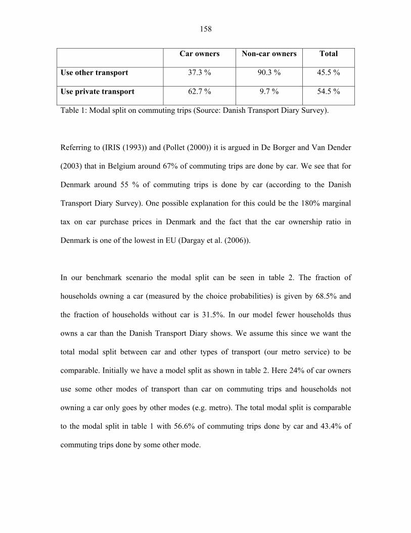
158

Car owners Non-car owners Total

Use other transport 37.3 % 90.3 % 45.5 %

Use private transport 62.7 % 9.7 % 54.5 %

Table 1: Modal split on commuting trips (Source: Danish Transport Diary Survey).

Referring to (IRIS (1993)) and (Pollet (2000)) it is argued in De Borger and Van Dender

(2003) that in Belgium around 67% of commuting trips are done by car. We see that for

Denmark around 55 % of commuting trips is done by car (according to the Danish

Transport Diary Survey). One possible explanation for this could be the 180% marginal

tax on car purchase prices in Denmark and the fact that the car ownership ratio in

Denmark is one of the lowest in EU (Dargay et al. (2006)).

In our benchmark scenario the modal split can be seen in table 2. The fraction of

households owning a car (measured by the choice probabilities) is given by 68.5% and

the fraction of households without car is 31.5%. In our model fewer households thus

owns a car than the Danish Transport Diary shows. We assume this since we want the

total modal split between car and other types of transport (our metro service) to be

comparable. Initially we have a model split as shown in table 2. Here 24% of car owners

use some other modes of transport than car on commuting trips and households not

owning a car only goes by other modes (e.g. metro). The total modal split is comparable

to the modal split in table 1 with 56.6% of commuting trips done by car and 43.4% of

commuting trips done by some other mode.

159

Car owners Non-car owners Total

Use other transport 24.0% 100.0% 43.4%

Use private transport 76.0% 0.0% 56.6%

Table 2: Modal split on commuting trips in base scenario.

The model is calibrated so that in the benchmark case the car ownership elasticity with

regards to fixed cost of purchasing a car is -0.20 which is numerically higher than the

estimates from Dargay (2001) where a long term elasticity of -0.11 is found52. Fosgerau

et al. (2004) estimate a short term elasticity of -0.19 and a long term elasticity of -0.48 for

Denmark. With the high tax on cars in Denmark we would expect the elasticity to be

numerically higher in Denmark than in the UK which is also confirmed by the findings in

Fosgerau et al. (2004). The car ownership elasticity with regards to variable transport cost

(i.e. fuel price) is our benchmark case -0.19 which is numerically higher than those found

in Dargay (2002) where the long run fuel cost elasticities is found to be between -0.14

and -0.06. Fosgerau et al. (2004) again reports values for Denmark which are numerically

higher than those reported by Dargay. They find a short term elasticity of -0.22 and a

long term elasticity of -0.55 with regards to user cost. The car transport elasticity with

regards to the fuel price in our baseline scenario is -0.17 which is in line with the fuel

price elasticity of -0.14 found in Nielsen (2006c) and Dargay (2004) find a long run fuel

cost elasticity for car travel to be between -0.18 and -0.10. Fosgerau et al. (2004) find the

short term elasticity with regards to running costs of car use to be -0.30 and a long term

elasticity to be -0.37. The car transport elasticity with regards to car purchase cost is in 52 In Dargays paper the elasticity depend on the number of cars per household. The elasticity of -0.09 applies when the number of cars per household is 1.2. If the number of cars is 1.0 the elascitity is found to be -0.11 and if the number of cars per household is 1.5 the elasticity is -0.07.

160

our model -0.08. This is numerically much lower than the findings in Nielsen (2006c)

where a long run elasticity of -1.13 is found for the entire country. Dargay (2004) find

long run elasticities between -0.62 and -0.43 which is closer to our value than the finding

in Nielsen (2006c). Since the values from Dargay (2004) and the value of -1.13 in

Nielsen (2006c) is found on a national level it is interesting that Nielsen (2006c) also

examines rural and urban households separately. He finds an insignificant effect of the

car purchase price on the travel demand in urban areas. This finding would call for a very

low elasticity to apply for these and we can thus se our model as being calibrated to fit a

situation in for example Copenhagen where a metro is also present. The labor supply

elasticity is chosen to be 0.5 which is in line with the reported values in Fuchs et al.

(1998).

In the situation where no congestion exists we have specified the speed-flow function

(58) such that the use of public transport takes 50% longer than transport by car. In the

basic scenario congestion exist and the use of public transport only takes 20% longer than

car transport. Furthermore we have specified the tax system so that a very high tax exists

on the purchase of cars (in our model 180%) and a fairly high tax exists on the use of cars

(in our model 100%). Furthermore car owners supply approximately 7.8 hours of work

per day and those who do not own a car supply approximately 5.9 hours of work per day

with an average working day of 7.2 hours in the economy. With an official working week

of 37 hours the average working time for Denmark is 7.4 hours and since we do expect

car owners to work more than those households who do not own a car, we find our model

to be well specified with regards to the time allocation. Using (12) and (25) to derive the

161

value of time for car owners and non-car owners we find that 0VoT is approximately

equal to 48% of the gross wage and 1VoT is approximately equal to 64% of the gross

wage. Expecting the value of time to be close to the after-tax wage rate we find these

values to be reasonable since the tax on labor in the model is 50% and since we expect

car owners to have a higher value of time than people not owning a car.

4.3 Shifting from fixed to variable taxes on cars

Labeling our base scenario as SC0 we now analyze two tax reforms (SC1 and SC2)

involving a reduction of the fixed tax on the purchase of cars in a budget-neutral way.

The first reform (SC1) reduces the tax on the purchase of cars from 180% to 170%

financing it by increasing the tax on the use of cars. The second reform (SC2) reduces the

taxation of cars to 100% again financing it by increasing the tax on the use of cars. The

modal split before and after the reforms can be found in table 3.

SC0 SC1 SC2

Car owners (% of population)

Use private transport (car)

Use public transport (metro)

Non-car owners (% of population)

Use other transport

Use private transport

Total modal split

Use private transport (car)

Use public transport (metro)

68.5 %

76.0 %

24.0 %

31.5 %

100.0 %

0.0 %

56.6 %

43.4 %

68.6 %

75.8 %

24.2 %

31.4 %

100.0 %

0.0 %

56.5 %

43.5 %

68.8%

74.2%

25.8 %

31.2%

100.0 %

0.0 %

55.3%

44.7%

Table 3: Modal split before and after the tax reforms

162

We see that more households purchase a car which is expected since the purchase price

goes down. We also see that the modal split shifts away from the use of cars to other

modes. If the elasticity was higher in the model we could end up in a situation where both

the number of car owners and the use of cars increase thus reversing the effect on the

modal split. The tax reforms also affect other parts of the economy. The changes in the

tax system, the change in labor supply, and the change in welfare is shown in table 4.

SC1 SC2

Taxes

Change in car purchase tax (relative to SC0)

Change in tax on car use (relative to SC0)

Effect on travel time by car (relative to SC0)

Effect on the labor supply

For non-car owners (relative to SC0)

For car owners (relative to SC0)

Total effect on labor supply (relative to SC0)

The welfare effect (relative to SC0)

-5.56%

7.20%

-0.40%

0.00%

-0.10%

-0.07%

0.005%

-44.44%

59.20%

-2.40%

0.00%

-0.85%

-0.58%

0.034%

Table 4: Changes in the tax system, travel time by car, and labor supply.

What we see from table 4 is that the reforms reduce the travel time by car. Furthermore

the effect on labor supply is interesting since our model shows that implementing a tax

reform like the one proposed here will reduce labor supply. This finding is in line with

results found elsewhere since increased taxation of commuting reduce the value of

163

working and thus discourage the supply of labor. Had the model not incorporated the

discrete nature of car ownership decision the conclusion could have been that the

reduction in labor supply would be closer to 0.85% but since we have households who

change car-ownership status and thus starts supplying more labor since car owners work

more., the reduction in labor supply could have been higher.

We also see that the tax reform actually improves welfare. It is however not clear if

welfare will continue to increase if the fixed tax is reduced even further. In order to

examine this we simulate a series of reforms which gradually reduce the fixed tax from

180% to 20%. The change in welfare when the taxes changes are shown in figure 1,

figure 2. In the figures the full line comes from the model and we also show best fit of a

high degree polynomial approximation to these results.

0,00%

0,01%

0,01%

0,02%

0,02%

0,03%

0,03%

0,04%

0,04%

0,05%

180%

170%

160%

150%

140%

130%

120%

110%

100% 90

%80

%70

%60

%50

%40

%30

%20

%

Fixed tax on the purchase of cars

Welfare effect

Figure 1: Change in welfare at different levels of the fixed tax relative to the welfare

when the tax is 180%.

164

0,00%

0,01%

0,01%

0,02%

0,02%

0,03%

0,03%

0,04%

0,04%

0,05%

0% 7% 14%

22%

29%

36%

44%

51%

59%

67%

75%

83%

91%

100%

108%

117%

126%

Change in variable tax on car transport

Welfare effect

Figure 2: Change in welfare when the tax on car transport is increased relative to the tax

in SC0.

Figure 1 shows that as the tax on purchase of cars decrease the welfare increase to a point

around 70% at which point we can see in figure 2 that the variable tax have increased

with around 85% (to approximately 190% in our model). One could speculate if this

external damage cost in this point is below, above or exactly equal to the tax rate

imposed. To examine this we specify the model in such a way that the variable tax is

given by 11 '

c

cTMt Z Lλ

λ= , keeping the budget balanced, and adjusting the fixed tax

accordingly. By doing so we find that a variable tax of 199% is internalizing the

externalities and the resulting fixed tax will be set equal to 50%. Using the model to

examine how welfare changes around this ‘pigouvian point’ we conclude that the

165

implementation of pigouvian taxation is the optimal choice if a tax reform which shifts

taxes from purchase of cars to use of cars are to be implemented.

-8,00%

-7,00%

-6,00%

-5,00%

-4,00%

-3,00%

-2,00%

-1,00%

0,00%

180%

170%

160%

150%

140%

130%

120%

110%

100% 90

%80

%70

%60

%50

%40

%30

%20

%

Fixed tax on the purchase of cars

%-change

Change inlabor supply

Change intraveltime bycarChange incar trips

Figure 3: Change in some key parameters relative to SC0 when the fixed tax is reduced.

The effect of such reform on other key variables can be seen in table 3. As in figure 1 we

depict the effect of the reduced purchase tax. We see that if we reduce this to 50% (the

pigouvian case) the labor supply will fall by approximately 1% and the travel time on car

trips will be reduced with around 4.5%. The number of car trips falls with approximately

5%.

5. Concluding remarks

This paper shows that the decision on the extensive margin (e.g., of car ownership), is an

important element in welfare evaluation of tax reforms in the transport sector. Omission

166

of decisions on the extensive margin could therefore be critical. Using a simple model for

household decisions, taxation, and discrete choice, we show how the feedback effect as

well as the welfare effect depends on the ownership decision and on the interaction with

the labor supply decision. We illustrated the effects in a small numerical model showing

that if we choose to implement a balanced budget tax reform which shifts taxes from car

ownership (or purchase) to car use it is optimal to implement pigouvian taxation.

Several extensions to this model can be envisioned. Including only commuting is not

satisfactory and leisure trips ought to be included. This extension could possibly be

implemented following the ideas of De Borger and Van Dender (2003). One could also

wish for more than two types of transport with different levels of fixed taxes to be

allowed for. This extension is straight forward to implement in the discrete setup

presented here and it would probably not influence the theoretical results. The simulation

used here should also be improved by calibrating it toward a specific city with

specifically obtained parameters and tailor made speed-flow functions for different types

of transport. Interaction between different transport modes could also be wished for since

congestion on the streets affects the travel time by bus but probably still leaves a metro

system unaffected. All these shortcomings will be left for future research and we still

believe that the findings of this paper will benefit future modeling of transport tax

reforms.

167

References

Becker, G. (1965) A Theory of the Allocation of Time, The Economic Journal 75, 493-

517.

Ben-Akiva, M. and Lerman, S. R (1985) Discrete Choice Analysis: Theory and

Application to Travel Demand, The MIT Press, Cambridge, Massachusetts.

Traffic Assignment Manual, Urban Planning Division, US Department of Commerce,

Washington DC.

Dargay, J., Hivert, L. and Legros, D. (2006) The dynamics of car ownership in E.U

countries: a comparison based on the european household panel survey, unpublished

working paper.

De Borger, B. (2000) Optimal two-part tariffs in a model of discrete choice, Journal of

Public Economics 76, 127-150.

De Borger, B. (2001) Discrete choice models and optimal two-part tariffs in the presence

of externalities: optimal taxation of cars, Regional Science and Urban Economics 31,

471-504.

De Borger, B. & Van Dender, K. (2003) Transport tax reform, commuting, and

endogenous values of time, Journal of Urban Economics 53, 510-530.

De Jong, G. C. (1990) An Indirect Utility Model of Car Ownership and Private Car Use,

European Economic Review 34, 971-985.

DeSerpa, A. C. (1971) A Theory of the Economics of Time, The Economic Journal 81,

828-846.

DØRS (2006) Dansk Økonomi, forår 2006, Det Økonomiske Råd, www.dors.dk.

168

Fosgerau, M., Holmblad, M. and Pilegaard, N. (2004) ART – En aggregeret

prognosemodel for dansk vejtrafik, Notat 5 2004, Danish Transport Research Institute.

McFadden, D. (1974) The measurement of urban travel demand, Journal of Public

Economics 3:4, 303-328.

Nielsen, J. E. (2006a) Taxation, Time Allocation, and Externalities, Thesis Paper.

Nielsen, J. E. (2006b) Real estate ownership and the demand for cars in Denmark – A

pseudo-panel analysis, Thesis Paper.

Nielsen, J. E. (2006c) Demand for car transport in Denmark – Differences between rural

and urban households, Thesis Paper.

Forsyth, P. J. (1980) The value of time in an economy with taxation, Journal of Transport

Economics and Policy 14:3, 337-362.

Fuchs, V. R., Krueger, A. B. & Poterba, J. M. (1998) Economists' Views about

Parameters, Values, and Policies: Survey Results in Labor and Public Economics,

Journal of Economic Literature 36, 1387-1425.

IRIS (1993) Region de Bruxelles-Capitale, Plan regional des Deplacements - Plan IRIS -

Constat et Scenario Tendanciel, Region de Bruxelles-Capitale.

Jara-Díaz, S. R. (2003) On the goods-activities technical relations in the time allocation

theory, Transportation 30, 245-260.

Parry, I. W. H. & Bento, A. (2001) Revenue Recycling and the Welfare Effects of Road

Pricing, Scandinavian Journal of Economics 103:4, 645-671.

Parry, I. W. H. & Bento, A. (2002) Estimating the Welfare Effect of Congestion Taxes:

The Critical Importance of Other Distortions within the Transport System, Journal of

Urban Economics 51, 339-365.

169

Pollet, I. (2000) Nationale Enquete over Mobiliteit van Huishoudens---Verslag van de

Eerste Analyse, Langzaam Verkeer, Leuven.

Small, K. A. & Rosen, H. S. (1981) Applied welfare economics with discrete choice

models, Econometrica 49, 105-130.

Small, K. A. (1992) Urban Transport Economics, Fundamentals of Pure and Applied

Economics Series, Harwood Academic Press, Philadelphia, USA.

Train, K. E. (2003) Discrete Choice Methods with Simulation, Cambridge University

Press.

Van Dender, K. (2003) Transport Taxes with Multiple Trip Purposes, Scandinavian

Journal of Economics 105:2, 295-310.